Higher order phase averaging for highly oscillatorysystems

Werner Bauer, Colin J. Cotter, Beth Wingate

July 9, 2021

Abstract

We introduce a higher order phase averaging method for nonlinear oscillatory sys-tems. Phase averaging is a technique to filter fast motions from the dynamics whilst stillaccounting for their effect on the slow dynamics. Phase averaging is useful for derivingreduced models that can be solved numerically with more efficiency, since larger timestepscan be taken. Recently, Haut and Wingate (2014) introduced the idea of computing finitewindow numerical phase averages in parallel as the basis for a coarse propagator for aparallel-in-time algorithm. In this contribution, we provide a framework for higher orderphase averages that aims to better approximate the unaveraged system whilst still filteringfast motions. Whilst the basic phase average assumes that the solution is independentof changes of phase, the higher order method expands the phase dependency in a basiswhich the equations are projected onto. We illustrate the properties of this method on anODE that describes the dynamics of a swinging spring due to Lynch (2002). Althoughidealized, this model shows an interesting analogy to geophysical flows as it exhibits a slowdynamics that arises through the resonance between fast oscillations. On this example,we show convergence to the non-averaged (exact) solution with increasing approximationorder also for finite averaging windows. At zeroth order, our method coincides with a stan-dard phase average, but at higher order it is more accurate in the sense that solutions ofthe phase averaged model track the solutions of the unaveraged equations more accurately.

Keywords: Phase averaging, slow-fast systems, resonant interactionsMSC2020: 37M99

1 Introduction

One of the main challenges in simulating highly oscillatory multiscale PDEs is that the fastwaves are known to create the lowest frequencies of the solution through nonlinear phase shifts,but are also responsible for severe linear wave time-step restrictions.

Phase averaging is a technique for approximating highly oscillatory systems so that thesolution still captures the long time trends in the dynamics Sanders et al. (2007). In thecontext of highly oscillatory nonlinear PDEs, the combination of coordinate transformation,phase averaging, and asymptotics has been used to derive slow PDEs that do this (Schochet,1994; Majda and Embid, 1998; Babin et al., 1997; Wingate et al., 2011, for example), providingrigorous derivations of slow geophysical models such as the quasigeostrophic model. Slow

1

arX

iv:2

102.

1164

4v2

[m

ath.

DS]

7 J

ul 2

021

models are more analytically tractable and easier to explain, and they are more efficient tosolve numerically. For an example numerical method inspired from the study of fast singularlimits see (Jones et al., 1999). The reason they are more tractable to solve is because theyhave had the fast frequencies filtered from them, and therefore much larger timesteps can betaken without excessively compromising stability or accuracy. For example, the first numericalweather prediction exercise by Charney, Fjortoft and von Neumann (Charney et al., 1950) wasbased upon the barotropic vorticity equation, a model that does not support the full gravityand pressure waves present in more detailed models. One problem with asymptotic models isthat they are only accurate at or near the limit, whereas the physically realistic parametersused in applications may not be near these limits, or the parameter regime itself may shiftas the simulation unfolds. Ongoing research in theoretical fluid dynamics highlights an issuewith using asymptotic equations that remove the fast oscillations: waves are responsible fortransfering the energy toward the low frequencies, see (Smith and Waleffe, 2002). This isone reason asymptotic models are not used in contemporary weather and climate modelingas a predictive tool. In fact, the role of the oscillations has been found to be key to allowingaccurate simulations and in some operational weather forcasting models, the compressible Eulerequations, which include sound waves, are used; for many years sound waves were thought tobe unimportant (Davies et al., 2003).

This paper is not about numerical algorithms, but it is highly motivated by them. Haut andWingate (2014) investigated the possibility of using a framework inspired by the study of fastsingular limits in that they use a coordinate transformation and phase averaging, but withoutasymptotics. They performed phase averaging over a finite window, and the phase averageintegral with numerical quadrature. Although this results in a computationally more intensivemodel, the terms in the quadrature sum can be evaluated independently, exposing possibilitiesfor parallel computing. The phase averaged formulation also involves the application of matrixexponentials, which can be computed by Krylov methods or other techniques such as the parallelrational approximation approach of Haut et al. (2016); Caliari et al. (2021); Schreiber et al.(2018), particularly suited to oscillatory operators. This produces a variant of heterogeneousmultiscale methods (Abdulle et al., 2012). The accuracy and stability of the finite window phaseaveraging technique was studied in Peddle et al. (2019), and applied to proving convergence ofthe parareal iteration. If the results of the averaging method are insufficiently accurate, thenit can be used as the predictor in a predictor-corrector framework, see (Jones et al., 1999, forexample). Many of these frameworks provide additional opportunities for parallel computing.With this in mind, Haut and Wingate (2014) introduced an asymptotic parareal method usingthe finite window averaging as a coarse propagator, and using a standard time integrationmethod applied to the original unaveraged system as a fine propagator.

In this paper we lay the foundations for an alternative approach, where the accuracy of thefinite window averaged model is increased “from the top down” by extending the phase averageinto a polynomial expansion of the solution in the phase variable. The goal is to further re-duce the error in the slow component of the solution whilst still filtering fast oscillations. Thisincreases the model complexity but it may be interesting to consider how to hide higher ordercorrections to the solution behind other computations in parallel, as occurs in the PFASSTframework (Minion, 2011), for example. Here, we introduce and explore the higher order aver-aging technique applied to ODEs, although we have highly oscillatory PDEs and fast singularlimits in mind when we do this. To isolate and understand the effects of our higher orderaveraging technique, in this paper we compute phase average integrals exactly (even though

2

practical approaches would use numerical quadrature), and we use an adaptive timestepper toget a very accurate estimate of the ODE solution trajectory. We find that when applied to aswinging spring model introduced by Lynch (Holm and Lynch, 2002), the higher order averag-ing does indeed produce a more accurate solution than the basic finite window averaging, andthat this error decreases as we increase the polynomial degree of the expansion in the phasevariable.

The rest of the paper is organised as follows. In Section 2 we introduce the higher orderaveraging technique in the most general form, before specialising to a polynomial basis for theexpansion in the phase variable as well as selecting a Gaussian averaging weight function sothat the phase averaging can be computed analytically. This is not critical to the frameworkbut was done to expediate our numerical experiments and to expose understanding of the effectof the higher order averaging. We then discuss asymptotic limits for the averaging window.In Section 3 we develop further formulae for Lynch’s swinging spring model, a specific lowdimensional example. In Section 4 we present numerical integrations for the swinging springexample, calculating errors between the higher order average models and the exact model.Finally, in Section 5 we provide a summary and outlook.

2 Higher order averaging: formulation

We consider initial value problems written in the following abstract form

∂

∂tU = LU +N(U,U), (2.1)

where L is a linear operator (with purely imaginary eigenvalues) and N is a nonlinear operator.Restricting ourselves to quadratic nonlinearities, we assume N to be a bilinear form (bilinearityindicated by the two slots). To develop phase averaged models, it is useful to reformulate (2.1)by introducing the factorization

V(t) = e−tLU(t), (2.2)

where the modulated variable V(t) satisfies the equation

∂

∂tV(t) = e−tLN

(etLV(t), etLV(t)

). (2.3)

We refer to this form as the modulated equation. It is straightforward to show that bothformulations are equivalent: when multiplying both sides of (2.1) with the integration factore−tL and noting that e−tL(∂tU− LU) = ∂t(e

−tLU), we recover Eqn. (2.3) via

e−tL(∂tU− tLU) = e−tLN(U,U)⇔ ∂t(e−tLU) = e−tLN(U,U) (2.4)

⇔ ∂tV = e−tLN(etLV, etLV). (2.5)

Note that this equation is valid for cases with or without scale separation (as discussed below).To apply phase averaging, we add an additional phase parameter s ∈ R over which we

integrate and hence average the solution. As a first step, we assume a factorization

V(t, s) = e−(t+s)LU(t) (2.6)

where, besides the time parameter t, we include a phase parameter s ∈ R in the exponentsuch that the solution in V depends on both t and s. The phase parameter s corresponds to

3

a change in the point where the exponential exp((t+ s)L) is equal to the identity, i.e. a phaseshift.

As a calculation similar to above shows, this factorization yields a form of (2.3) that includesthe parameter s, i.e.

∂

∂tV(t, s) = e−(t+s)LN

(e(t+s)LV(t, s), e(t+s)LV(t, s)

). (2.7)

This gives us a one parameter family of solutions V(t, s) that depend on the phase parameters with the property that for s = 0 we recover the solution of (2.3). We can then obtain a phaseaveraged model,

∂

∂tV(t) = lim

T→∞

1

2T

∫ T

−Te−(t+s)LN

(e(t+s)LV(t, s), e(t+s)LV(t, s)

)d s. (2.8)

Phase averaging for (2.7) was analysed by Schochet (1994) in the limit ε → 0, leading toslow equations that approximate the solution of the unaveraged model in this limit in someappropriate sense. In particular, Majda and Embid (1998) showed that this averaging and ε→ 0limit recovers the quasigeostrophic equation in the low Rossby number limit of the rotatingshallow water equations, when written in this form. For finite Rossby number, Haut andWingate (2014) proposed to adapt this approximation to numerical computations by keepingT finite and introducing a C∞ weight function ρ with ρ ≥ 0, ‖ρ‖L1 = 1, to obtain the averagedequation

∂

∂tV(t) =

∫ ∞−∞

ρT (s) e−(t+s)LN(e(t+s)LV(t, s), e(t+s)LV(t, s)

)d s, (2.9)

where ρT (s) = ρ(s/T )/T . They further proposed to replace the integral via quadrature (choos-ing ρ to have compact support), with the evaluation of the integrand at each quadrature pointbeing computed independently in parallel; this formulation provided the coarse propagator fora parallel-in-time algorithm.

Note that depending on the value of T , formulation (2.9) recovers an averaged version, anasymptotic approximation, or the full equations (2.3):

• for T → 0, we recover Eqn. (2.3) because in the limit T → 0 the weight function ρconverges formally to the Dirac measure δ(s).

• for T → ∞, we recover (2.9), because when integrating the resulting integral value isinvariant under shifts in t; hence for t = 0 we recover the asymptotic approximationintroduced in Majda and Embid (1998) after also taking ε→ 0.

• for 0 << T <<∞, formulation (2.9) has a smoothing effect on fast oscillations with timeperiod less than T .

The optimum choice of T as a function of ε to minimise the error due to averaging whencombined with a numerical time integration method to solve (2.9) was investigated in Peddleet al. (2019).

An interpretation of (2.9) is that we have projected V(t, s) onto the space of functionsindependent of s using the ρ-weighted L2 inner product. In the next subsection, our higherorder averaging method for finite averaging window T will be based on projecting the oneparameter family of solutions on to higher order polynomials in s. After solving this system of

4

coupled differential equations, we set s = 0 because we are interested only in the time evolutionof the solution with this phase value. Hence, we only present solutions at s = 0 in the numericalresults section.

2.1 General framework of higher order time averaging

We abbreviate the RHS of (2.3) as general bilinear function F(V(t, s),V(t, s); t + s) that hasquadratic dependency on V(t, s), i.e.

∂

∂tV(t, s) = F

(V(t, s),V(t, s); t+ s

). (2.10)

According to (2.6), the solution vector V depends on both t and s and we assume that it canbe represented by the factorization

V(t, s) =

p∑k=0

Vk(t)φk(s), (2.11)

where φk(s) are basis vectors depending on s that span Q, some chosen (p + 1)-dimensionalfunction space.

We project (2.10) onto Q to obtain∫ ∞−∞

ρT (s)W(s) · ∂∂t

V(t, s)ds =

∫ ∞−∞

ρT (s)W(s) · F(V(t, s),V(t, s); t+ s

)ds ∀W(s) ∈ Q,

(2.12)where ρT (s) = ρ(s/T )/T for our chosen weight function ρ.

Also expanding the test function W in the basis,

W(s) =

p∑j=0

Wjφj(s), (2.13)

we get

p∑j=0

p∑k=0

Wj

∫ ∞−∞

1

Tρ( sT

)φj(s)φk(s)ds

∂

∂tVk(t) =

p∑j=0

Wj

∫ ∞−∞

1

Tρ( sT

)φj(s)F

( p∑k=0

Vk(t)φk(s),

p∑l=0

Vl(t)φl(s); t+ s)ds, ∀W1, . . . ,Wp.

(2.14)

As the coefficients Wj are independent from each other, we obtain

p∑k=0

∫ ∞−∞

1

Tρ( sT

)φj(s)φk(s)ds

∂

∂tVk(t) =

∫ ∞−∞

1

Tρ( sT

)φj(s)F

( p∑k=0

Vk(t)φk(s),

p∑l=0

Vl(t)φl(s); t+ s)ds.

(2.15)

5

This defines our averaged model for the components Vk, in the form of a matrix-vector equationfor ∂

∂tVk. To use it, we set V(t = 0, s) = U(0), the initial condition, independently of s. Then

we solve the equations forward in time (perhaps approximating the phase integral as a sum),taking the solutions at s = 0.

To understand more about what this approximation does, we further specify the nonlinearfunction F. As it is bilinear, we may pull out the double sum over the basis φ, i.e.

F

(p∑

k=0

Vk(t)φk(s),

p∑l=0

Vl(t)φl(s); t+ s

)=

p∑k=0

p∑l=0

φk(s)φl(s)F(Vk(t),Vl(t); t+ s

). (2.16)

Moreover, we assume that we can factor out the time dependency of F on t + s so that F isrepresented as

F(Vk(t),Vl(t); t+ s

)=∑m

Fm

(Vk(t),Vl(t)

)ei(t+s)cm (2.17)

where the sum in m is over different terms that are quadratic in V (for different polynomialorder k, l) with coefficients cm and bilinear functions Fm and that depend on the nonlinearoperator N . In the case of a PDE, this sum over m will be replaced by an infinite sumover frequencies. Examples of these coefficients and their relations are shown further belowin Table 3.1 for the swinging spring model. To ease notation, we will adopt the short handnotation Fm,k,l(t) := Fm

(Vk(t),Vl(t)

).

In summary, we end up with a system of equations (for j = 0, . . . p) that reads

p∑k=0

∫ ∞−∞

1

Tρ( sT

)φj(s)φk(s)ds

∂

∂tVk(t) =

∑m

p∑k=0

p∑l=0

Fm,k,l(t)

∫ ∞−∞

1

Tρ( sT

)φj(s)φk(s)φl(s)e

i(t+s)cmds ∀φj(s).(2.18)

This formulation provides a general framework of higher order averages for various choices ofQ and weight function ρ.

2.2 Polynomial higher order time averaging

In this section we make some specific calculations using the choice of Q = Pp, the degree-p polynomials, and a particular choice of weight function that allows us to make progressanalytically, namely ρ(s) = exp(−s2/2)/

√2π, recalling that∫ ∞

−∞

1

Tρ( sT

)ds =

∫ ∞−∞

1√2πT 2

e−s2

2T2 ds = 1. (2.19)

This allows us to integrate over the whole R while guaranteeing a bounded integral, but otherchoices are possible too.

As a basis φ, we choose the standard monomials

φj(s) = sj, j = 0, . . . , p. (2.20)

This is a poorly-conditioned basis, and better choices might be made for large values of p (forthe weight function we are using the Hermite polynomials would be ideal since they diagonalise

6

the mass matrix). However, the monomial basis simplifies the calculations below. Also, underthis basis, V(t, s = 0) = V0(t), so to initialise the system we can just set V0(0) = V(0, s = 0)and Vk(0) = 0 for 1 ≤ k ≤ p.

Substituting this basis into (2.18), we arrive at

p∑k=0

1√2πT 2

∫ ∞−∞

e−s2

2T2 sjskds∂

∂tVk(t) =

∑m

p∑k=0

p∑l=0

Fm,k,l(t)eicmt

1√2πT 2

∫ ∞−∞

e−s2

2T2 eicmssjskslds ∀j.(2.21)

The latter equation can be formulated more concisely as

p∑k=0

Mjk∂

∂tVk(t) =

∑m

p∑k=0

p∑l=0

Fm,k,l(t)eicmtRm

jkl ∀j, (2.22)

in which we denote the integral on the left hand side (LHS) of (2.21) as a mass matrix

Mjk =1√

2πT 2

∫ ∞−∞

e−s2

2T2 sjskds, (2.23)

and that on the RHS of (2.21) as

Rmjkl =

1√2πT 2

∫ ∞−∞

e−s2

2T2 eicmssjskslds. (2.24)

To evaluate these integrals, it will be useful to introduce the notation

Iα :=1√

2πT 2

∫ ∞−∞

e−s2

2T2 sαds (2.25)

with I0 = 1 which follows immediately from (2.19). Then, for instance, for α = i + j we haveMij = Iα. With the help of this concise notation, we formulate the following two propositionsthat allow us to evaluate the integrals in (2.23) and (2.24).

Proposition 2.1. For averaging window T and α = j + k with j, k = 0, . . . , p, the integral Iαin (2.25) can be represented in the recursive form

Iα = T 2(α− 1)Iα−2 with I0 = 1 (2.26)

In particular, Iα = 0 for all α odd.

Proof. This recursive formula follows directly from integration by parts. Using the normaliza-tion factor γ = 1√

2πT 2, there follows

Iα = γ

∫ ∞−∞

d

dse−

s2

2T2−2T 2

2ssαds = γ

[−e−

s2

2T2 T 2sα−1]∞−∞

+ T 2(α− 1)γ

∫ ∞−∞

e−s2

2T2 sα−2ds

= T 2(α− 1)Iα−2.

(2.27)

For α = 0, we have I0 = 1 since∫∞−∞ e

− s2

2T2 =√

2πT 2 which follows from (2.19). For odd α, Iαis an integral of a product of an even and odd function over entire R, hence zero.

7

Proposition 2.2. Using the recursive formula of Proposition 2.1 and for averaging window Tand α = j + k + l with j, k, l = 0, . . . , p, the integral (2.24) can be represented for all m as

Rmα = e−

c2mT2

2 Rmα with Rm

α =α∑β=0

(α

β

)Iα−β · (icmT 2)β (2.28)

with the property that for α = 0 we have Rm0 = 1 for all m.

Proof. First, we rewrite (2.24) using α = j+k+ l and by completing the square (− s2

2T 2 + icms =

− 12T 2 (s− icmT 2)2 − c2mT

2

2) we arrive at

Rmα = e−

c2mT2

2 Rmα with Rm

α :=1√

2πT 2

∫ ∞−∞

e−1

2T2 (s−icmT 2)2sαds. (2.29)

Next, we use the substitution s′ = s− icmT 2 with ds′ = ds:

Rmα =

1√2πT 2

∫ ∞−icmT 2

−∞−icmT 2

e−s′22T2 (s′ + icmT

2)αds′. (2.30)

Because the latter is a contour integral in the complex domain in which one term is integratedalong the real axis and another one along a semi circle at infinity, the shift of the real axis inthe complex direction by −icmT 2 does not change the integral value as long as there are no, orthe same number of singularities enclosed by the contour. Therefore, we can equivalently write

Rmα =

1√2πT 2

∫ ∞−∞

e−s′22T2 (s′ + icmT

2)αds′ (2.31)

while for α = 0 there follows

Rm0 =

1√2πT 2

∫ ∞−icmT 2

−∞−icmT 2

e−s′22T2 ds′ =

1√2πT 2

∫ ∞−∞

e−s′22T2 ds′ = 1. (2.32)

For the ease of notation, we will skip ′ in the following. Using the binomial expansion (x+y)α =∑αβ=0

(αβ

)xα−βyβ, Eqn. (2.31) becomes

Rmα =

α∑β=0

(α

β

)(1√

2πT 2

∫ ∞−∞

e−s2

2T2 sα−βds

)(icmT

2)β. (2.33)

The statement follows by using expression (2.26) for the term in brackets.

Based on these results, we can further expand (2.22) to get

p∑k=0

Mjk∂

∂tVk(t) =

∑m

p∑k=0

p∑l=0

Fm,k,l(t)Rmjkle

icmte−c2mT2

2 for j = 0, 1, 2, (2.34)

where Mjk = Mα for α = j + k and Rmjkl = Rm

α for α = j + k + l. Note that Fm,k,l = Fm,l,k forall m, k, l.

Equation (2.34) will serve us in Section 3 to develop a higher order averaging method for anODE describing a swinging spring. But before we discuss this example, let us first present anexplicit representation of (2.34) and how the equation behaves in the zero and infinity limitsof T .

8

2.2.1 Explicit representation for polynomial order p = 2

For the sake of clarity, we present an explicit representation of Eqn. (2.34) for p = 2, i.e.j, k, l = 0, 1, 2. Proposition 2.1 leads to a mass matrix M with coefficients (in terms of Mα):

M0 = 1, M1 = 0, M2 = T 2, M3 = 0, M4 = 3T 4; (2.35)

and we can explicitly write the inverse of M as

M−1 =

1 0 T 2

0 T 2 0T 2 0 3T 4

−1 =

32

0 −12T 2

0 1T 2 0

−12T 2 0 1

2T 4

. (2.36)

Moreover, Proposition 2.2 leads to the coefficients (in terms of Rmα ):

Rm0 = 1, Rm

1 = icmT2, Rm

2 = T 2 − c2mT 4, Rm3 = i3cmT

4 − ic3mT 6,

Rm4 = 3T 4 − 6c2mT

6 + c4mT8, Rm

5 = i15cmT 6 − i10c3mT8 + ic5mT

10,

Rm6 = 15T 6 − 45c2mT

8 + 15c4mT10 − c6mT 12.

(2.37)

With these coefficients, the explicit form of Eqn. (2.34) readsM00 0 M02

0 M11 0M20 0 M22

V0(t)

V1(t)

V2(t)

=∑m

2∑k=0

2∑l=0

eicmte−c2mT2

2 Fm,k,l

Rm0kl

Rm1kl

Rm2kl

=∑m

eicmte−c2mT2

2 ×[Fm,0,0

Rm000

Rm100

Rm200

+ Fm,0,1

Rm001

Rm101

Rm201

+ Fm,0,2

Rm002

Rm102

Rm202

+ Fm,1,0

Rm010

Rm110

Rm210

+ Fm,1,1

Rm011

Rm111

Rm211

+ Fm,1,2

Rm012

Rm112

Rm212

+ Fm,2,0

Rm020

Rm120

Rm220

+ Fm,2,1

Rm021

Rm121

Rm221

+ Fm,2,2

Rm022

Rm122

Rm222

].(2.38)

Bringing M to the LHS, we result inV0(t)

V1(t)

V2(t)

=∑m

2∑k=0

2∑l=0

eicmte−c2mT2

2 Fm,k,l

32

0−12T 2

Rm0kl +

01T 2

0

Rm1kl +

−12T 2

01

2T 4

Rm2kl

.

(2.39)

As it is useful for the asymptotic study further below, we present a fully explicit version of (2.39)in terms of tendencies for V0, V1, and V2 in Appendix A. This explicit representation illustratesclearly the coupling between the principal V0 term and the higher order ones Vi, i = 1, . . . pand allows us to visualize the expansion’s asymptotic behavior with respect to the averagingwindow T . Here we explicitly see the smoothing effect for large averaging window T , as all ofthe terms are exponentially small in T except for resonant cases where cm is small.

9

2.2.2 Asymptotic behaviour with respect to T

We illustrate the asymptotic behavior of the expansion (2.39) on the example presented abovefor p = 2, but the results hold for general p. In particular, we investigate its behaviour forlarge and small T , which can be inferred from an explicit representation of (2.39), as shownin Appendix A. Here, we present a general discussion while showing a concrete example inSection 3.

Limit T → 0: We study equation (2.39) in the limit T → 0. In this limit, many terms vanish(cf. Appendix A) and we arrive atV0(t)

V1(t)

V2(t)

=∑m

eicmt ×

Fm,0,0

icmFm,0,0 + 2Fm,0,1

−12c2mFm,0,0 + Fm,1,1 + 2icmFm,0,1 + 2Fm,0,2

. (2.40)

In the limit T → 0 the higher order coefficients thus decouple from the lowest order coefficientV0, i.e. V0 does not depend on the higher order terms. When considering only V0, which isall that we are interested in, we recover in fact the non-averaged equation (2.3).

Remark 2.3. Considering the full system (2.40), higher order terms do not vanish and in thenumerical algorithm below, these terms will be calculated too. However, for T very small, thecondition number of matrix M is very large leading to increased numerical errors (cf. discussionto Figure 4.4). In practice this can be dealt with by choosing a better conditioned basis suchas an orthogonal basis with respect to the ρ-weighted inner product (which would be Hermitepolynomials in the examples we have computed here). However, this only becomes an issuein the small T limit, and we are interested in larger T values to facilitate larger timesteps innumerical integrations.

Limit T → ∞: We study expansion (2.39) for T → ∞. To this end, we have to distinguishbetween the terms in the sum on the RHS of (2.39) with coefficients (i) cm 6= 0 and (ii) cm = 0(see e.g. the coefficients in Table 3.1).

Case 1: for cm 6= 0 there follows eicmte−c2mT2

2 = 0 for T → ∞ such that the correspondingterms on the RHS of (2.39) are zero (cf. Appendix A).

Case 2: for cm = 0 there follows eicmte−c2mT2

2 = 1 for any T . Hence, not all terms on theRHS vanish (cf. Appendix A) and we arrive at the following equation:V0(t)

V1(t)

V2(t)

=∑m

Fm,0,0 − 3T 4Fm,2,2

2Fm,0,1 + 6T 2Fm,1,2

Fm,1,1 + 2Fm,0,2 + 6T 2Fm,2,2

. (2.41)

Similar to the zero limit (2.40), there is a decoupling of the higher order modes from the principleone: the Fm,0,0 term vanishes in the higher order modes. Therefore, as all Vi, i = 1, ..p areinitialized with zero, they remain zero including the Fm,2,2 that would contribute otherwise toV0. Therefore, we recover indeed in this limit an asymptotic approximation of (2.3) in form ofMajda and Embid (1998).

10

3 Example ODE: swinging spring

We illustrate the properties of the higher order averaging method introduced above on an ODEthat describes the dynamics of a swinging spring, a model due to Peter Lynch (Holm and Lynch,2002). Although idealized, this model shows an interesting analogy to geophysical flows as itexhibits a high sensitivity of small scale oscillation on the large scale dynamics.

3.1 The swinging spring

For the swinging spring (expanding pendulum) model of Holm and Lynch (Holm and Lynch,2002), we consider the following equations of motion

x(t) + ω2Rx(t) = λx(t)z(t),

y(t) + ω2Ry(t) = λy(t)z(t),

z(t) + ω2Zz(t) = 0.5λ(x(t)2 + y(t)2),

(3.1)

where x(t), y(t), z(t) are (time dependent) Cartesian coordinates centered at the point of equi-librium, ωR =

√g/l is the frequency of linear pendular motion, and ωZ =

√k/mu is the

frequency of elastic oscillation with spring constant k, unit mass mu and gravitational constantg. l0 denotes the unstretched length while l is the length at equilibrium such that λ = l0ω

2Z/l

2.The dot denotes the time derivative d

dt.

To bring Eqn. (3.1) into the abstract form (2.1), we first reformulate the former into thefirst order system

x(t)− ωRpx(t) = 0, px(t) + ωRx(t) =λ

ωRx(t)z(t),

y(t)− ωRpy(t) = 0, py(t) + ωRy(t) =λ

ωRy(t)z(t),

z(t)− ωZpz(t) = 0, pz(t) + ωZz(t) =λ

ωZ(x(t)2 + y(t)2),

(3.2)

with px := ∂p∂x

and so forth. Then, by introducing the complex numbers X(t) = x(t) +ipx(t), Y (t) = y(t) + ipy(t), Z(t) = z(t) + ipz(t), we can rewrite Eqn. (3.2) as

X(t) + iωRX(t) = iλ

ωRRe(X(t))Re(Z(t)), (3.3)

Y (t) + iωRY (t) = iλ

ωRRe(Y (t))Re(Z(t)), (3.4)

Z(t) + iωZZ(t) = iλ

2ωZ(Re(X(t))2 +Re(Y (t))2). (3.5)

This form of the equations can be expressed in the abstract form (2.1) by defining the velocityas

U(t) =

X(t)Y (t)Z(t)

=

x(t) + ipx(t)y(t) + ipy(t)z(t) + ipz(t)

, (3.6)

11

the linear operator as

L =

−iωR−iωR−iωRρ

, (3.7)

and the nonlinear (quadratic) operator as

N(U(t),U(t)) = iλ

ωR

Re(X(t))Re(Z(t))Re(Y (t))Re(Z(t))

ρ2(Re(X(t))2 +Re(Y (t))2)

. (3.8)

Using these definitions, Eqn. (3.1) can also be written in the modulated form (2.3). Thatis, the time evolution of the velocity V(t) with transformation

V(t) = e−tLU(t), V(t) =

X(t)

Y (t)

Z(t)

, (3.9)

under the linear operator L of (3.7) is given by Eqn. (2.3) with nonlinear operator N of (3.8).Explicitly, we arrive at the component equations:

˙X = cxyXZe

−iωRρt + cxyXZeiωRρt + cxyZXe

−iωRρt+2iωRt + cxyXZeiωRρt+2iωRt (3.10)

˙Y = cxyY Ze

−iωRρt + cxyY ZeiωRρt + cxyZY e

−iωRρt+2iωRt + cxyY ZeiωRρt+2iωRt (3.11)

˙Z = cz(X

2 + Y 2)eiωRρt−2iωRt + 2cz(XX + Y Y )eiωRρt + cz(X2

+ Y2

)eiωRρt+2iωRt (3.12)

with coefficients cxy = 3iωRρ2/16 and cz = 3iωRρ/32. Overline notation denotes the conjugate.

For ease of notation, we omitted here to include the time dependency of the transformedcomponents X, Y , Z. After solving for V, we have to transform back to U with U(t) = etLV(t)to find solutions of (2.1).

The explicit formulation in (3.10)–(3.12) allows us to identify the problem (or ODE) depen-dent coefficient cm and Fm,k,l = (F x

m, Fym, F

zm) ∀k, l of the expansion (2.34). Note that the latter

coefficients change with m while they are the same for all k, l. The following table summarizesthese coefficients:

cm F xm F y

m F zm

c1 := (ρ− 2)ωR 0 0 F z1 = cz(XX + Y Y )

c2 := ρωR F x2 = cxyXZ F y

2 = cxyY Z F z2 = 2cz(XX + Y Y )

c3 := (ρ+ 2)ωR F x3 = cxyXZ F y

3 = cxyY Z F z3 = cz(XX + Y Y )

c4 := −ρωR F x4 = cxyXZ F y

4 = cxyY Z 0

c5 := −(ρ+ 2)ωR F x5 = cxyXZ F y

5 = cxyY Z 0

Table 3.1: Coefficients of expansion (2.34) for the swinging spring model.

The coefficients from Table 3.1 are used in expansion (2.34) to obtain the higher order phaseaveraged system.

12

Limits for T : Similarly to Section 2 but here for concrete model equations, i.e. for theODE (3.1) of the swinging spring, we present the equations describing the time evolution of V0

resulting from taking the limits of (2.34) in T , i.e. for (i) T → 0 and (ii) T →∞.Case (i): as discussed in (2.40), in the T to zero limit the higher order terms decouple

from the principle mode V0 such that for the time evolution of the latter only the Fm,0,0 termscontribute. In this limit and using the coefficients of Table 3.1, the resulting set of equationsfor V0 coincides with equations (3.10)–(3.12) of the exact model.

Case (ii): as shown in (2.41), all terms on the RHS of the expansion (2.34) vanish in theT →∞ limit except of those with cm = 0 (i.e. here for ρ = 2). Considering further that higherorder terms in V (i.e. for k > 0 and/or l > 0) are initialized with zero, these terms, and inparticular the Fm,2,2 terms in the first line in (2.41), remain zero. Then, for any approximationorder p, the resulting set of equations for V0 are given by

˙X = cxyZX,

˙Y = cxyZY ,

˙Z = cz(X

2 + Y 2). (3.13)

This is exactly the phase-averaged model that was derived by Holm and Lynch (2002) usingWitham averaging.

4 Numerical results

We investigate accuracy and stability of the higher order phase averaging method on numericalsimulations of the swinging spring model as introduced in the previous section. We comparesolutions obtained from the approximated models with those from the non-averaged (exact)equations (2.3). In particular, the convergence behavior of solutions obtained from averagingmodels with increasing approximation order to exact solutions will be investigated for finiteaveraging windows. Besides showing that higher order phase averaging indeed leads to a betterapproximation of the fast oscillations around the slow manifold than standard (first order)averaging, we illustrate that this also reduces the drift from averaged solutions away from theexact solutions, which we experienced in our simulations.

Analogously to Holm and Lynch (2002), we choose for the numerical simulations the fol-lowing parameters for the ODE in equation (3.1): mu = 1 kg, l = 1 m, g = π2 m s−2, k = 4π2

kg s−2 and hence ωR = π and ωZ = 2π with resonance condition ωZ = 2ωR. The unstretchedlength l0 = 0.75 m follows from the balance k (l− l0) = g mu allowing us to determine λ in (3.1).Finally, the equations are initialized with

(X0(0), Y0(0), Z0(0)) = (0.006, 0, 0.012) m, (X0(0), Y0(0), Z0(0)) = (0, 0.00489, 0) m s−1,

for the principle mode V0 while values for V 6=0 and V 6=0 are all initialized with zero and resetback to zero after an integration window ∆T . This resetting avoids potential instabilities in thehigher order modes in Vi, i = 1, ...p (cf. discussion to Figure 4.2). If not stated otherwise, weuse a resetting window of ∆T = 100 s while other choices are also possible because this choicedoes not significantly impact on the accuracy of the solutions, as shown below in Figure 4.6.

Note that with this parameter choice, the fast and slow motions occurring in the simulationshave a scale separation at the order of about ε ≈ 0.01 (in good agreement with values forgeophysical flows).

13

0.02 0.01 0.00 0.01 0.02X0 [m]

0.02

0.01

0.00

0.01

0.02

Y 0 [m

]

exctavg, T=0.5HO p=6, T=0.5

0 25 50 75 100 125 150 175time t [s]

0.010

0.005

0.000

0.005

0.010

Z 0 [m

]

exctavg, T=0.5HO p=6, T=0.5

Figure 4.1: Left: horizontal projection of X0, Y0 components of pendulum movement for 1000 sfor the exact (exct), averaged (avg) and higher order (HO) averaged models. Right: Verti-cal projection of Z0 component of pendulum movement over time t for 167 s (correspondingapproximately to the first of six modulation cycles).

We integrate the ODEs in time using the adaptive RK4/5 explicit integrator implementedthrough the Python Scipy package. We integrate up to 1000 seconds (corresponding to 1000 ver-tical oscillations) using adaptive relative and absolute tolerance of 1.49012e−8 unless otherwisestated.

To ease notation, we consistently denote also solutions of the exact (equations (3.10)–(3.12))and the averaged (p = 0) models with U0 = (X0, Y0, Z0) and V0 = (X0, Y0, Z0) even thoughthere are no higher order terms present in these cases.

4.1 Large scale dynamics, smoothing behavior and stability

First, we verify that the solutions of our phase averaged models stay close to the correspondingexact solutions and capture the same characteristics typical to the swinging spring model (given,for instance, by the stepwise precision of the pendulum in the (x, y)-plane). To this end, wecompare for a long term simulation of 1000 s the solutions in U0 of the exact model, the averagedone with p = 0 that corresponds to Peddle et al. (2019) and a higher order (HO) version with,e.g., p = 6. In order to guarantee stable simulations, we reset the higher order values in Ui (orVi), i = 1, ...p, to zero, here after a resetting time of ∆T = 100 s. The size of this resettingwindow ∆T does only marginally impact the accuracy (cf. Figure 4.6) but resetting preventsthe averaged solutions to become unstable, in particular for large p and long simulations (cf.Figure 4.2).

Large scale dynamics. In Figure 4.1 (left) we see the projection of the pendulum movementonto the horizontal (x, y)-plane. Both, the solutions for the averaged and HO averaged modelsare very close to the exact solutions, almost indistinguishable in the given figures that showthe large scale dynamics. Here, we used an averaging window of T = 0.5 s while for smaller Tthe accuracy does increase (cf. e.g. Figure 4.5). In particular, the solutions of the averagedmodels capture very well the stepwise precision of the swinging spring model. In the right panel,the movement of the pendulum in the Z axis versus time is shown. Also here, both averaged

14

0 200 400 600 800 1000time t [s]

1.5

1.0

0.5

0.0

0.5

1.0

1.5

2.0

2.5

X0,

Y 0,Z

0 [m

]

1e 2

X0 exctX0 avgX0 HO X0 nores

Y0 exctY0 avgY0 HO Y0 nores

Z0 exctZ0 avgZ0 HO Z0 nores

Figure 4.2: X0, Y0, Z0 solutions of the exact (exct), averaged (avg with p = 0) and higher order(HO) models (with p = 8) and T = 0.2 s; reset every ∆T = 100 s or with no resetting (nores).Here, no resetting leads to instabilities for high p ≥ 8 after about 800 s.

and HO averaged solutions are very close to the exact one. The figure illustrates nicely fastoscillations with a slowly varying amplitude envelope. This typical behavior of the swingingspring model makes it thus a perfect test problem for our averaging method developed above.

Smoothing properties. Next, we illustrate how the proposed averaging algorithm filters fastmotions from the dynamics of the swinging spring model while still accounting for their effecton the slow dynamics. Given the factorization assumption (2.2) that underlies equations (2.3),it is useful to study in more detail solutions in terms of the velocity V because the latterprovide solutions of the slow dynamics without most of the fast oscillations intrinsic to U.As such, V (in particular V0) allows us to clearly illustrate how the averaging method filtersfast oscillations and how the higher order methods better approximate small scale oscillationsaround the slow dynamics.

Figure 4.2 shows the solutions for X0, Y0, Z0 of the exact, the averaged, and the HO averagedmodels without resetting and with resetting at ∆T = 100 s. We use an averaging window ofT = 0.2 s and p = 8 for the HO method as this provides sufficiently accurate solutions (cf.Figure 4.5). The figure illustrates also a solutions of the HO model for p = 8 (X0 nores,Y0 nores, Z0 nores) that becomes slightly unstable after about 800 s in case no resetting isused. This instability, however, is easily controlled by simple resetting the higher order velocitycomponent at each ∆T to zero, resulting in the stable solutions X0 HO, Y0 HO, Z0 HO.

Next, we compare the exact solutions in all three components with those of the averagedmodels. We realize that for longer simulation times, the averaged solutions slightly drift away

15

0.1 0.0 0.1 0.2 0.3 0.4 0.5 0.6time t [s]

5.970

5.975

5.980

5.985

5.990

5.995

6.000

6.005

X0 [

m]

1e 3

X0 exctX0 avgX0 HO p=1X0 HO p=2X0 HO p=3X0 HO p=4X0 HO p=5X0 HO p=6X0 HO p=7X0 HO p=8X0 HO p=9X0 HO p=10

998.0 998.5 999.0 999.5 1000.0 1000.5 1001.0time t [s]

5.35

5.40

5.45

5.50

5.55

5.60

X0 [

m]

1e 3

X0 exctX0 avgX0 HO p=1X0 HO p=2X0 HO p=3X0 HO p=4X0 HO p=5X0 HO p=6X0 HO p=7X0 HO p=8X0 HO p=9X0 HO p=10

0.2 0.0 0.2 0.4 0.6 0.8 1.0time t [s]

0.01

0.00

0.01

0.02

0.03

0.04

0.05

Y 0 [m

]

1e 3

Y0 exctY0 avgY0 HO p=1Y0 HO p=2Y0 HO p=3Y0 HO p=4Y0 HO p=5Y0 HO p=6Y0 HO p=7Y0 HO p=8Y0 HO p=9Y0 HO p=10

998.0 998.5 999.0 999.5 1000.0 1000.5 1001.0time t [s]

1.100

1.075

1.050

1.025

1.000

0.975

0.950

0.925

0.900Y 0

[m]

1e 3

Y0 exctY0 avgY0 HO p=1Y0 HO p=2Y0 HO p=3Y0 HO p=4Y0 HO p=5Y0 HO p=6Y0 HO p=7Y0 HO p=8Y0 HO p=9Y0 HO p=10

0.2 0.0 0.2 0.4 0.6 0.8 1.0time t [s]

11.980

11.985

11.990

11.995

12.000

12.005

Z0 [

m]

1e 3

Z0 exctZ0 avgZ0 HO p=1Z0 HO p=2Z0 HO p=3Z0 HO p=4Z0 HO p=5Z0 HO p=6Z0 HO p=7Z0 HO p=8Z0 HO p=9Z0 HO p=10

998.0 998.5 999.0 999.5 1000.0 1000.5 1001.0time t [s]

4.50

4.75

5.00

5.25

5.50

5.75

6.00

6.25

6.50

Z0 [

m]

1e 3

Z0 exctZ0 avgZ0 HO p=1Z0 HO p=2Z0 HO p=3Z0 HO p=4Z0 HO p=5Z0 HO p=6Z0 HO p=7Z0 HO p=8Z0 HO p=9Z0 HO p=10

Figure 4.3: X0, Y0, Z0 solutions of the exact (exct), averaged (avg with p = 0) and higher order(HO) models with resetting (∆T = 100 s) and averaging window T = 0.15 s.

from the exact ones, as shown on the right panels in Figure 4.3. This is particularly obviousin the Z0 component. Further in this figure, we see clearly that with increasing approximationorder p the solutions’ drift reduces significantly whilst the small scale oscillations are betterapproximated. Note that the standard averaging method with p = 0 corresponds to the originalversion as introduced in Haut and Wingate (2014). As discussed therein, the averaging leadsto some drift away from the exact solutions. As the figure illustrates clearly, including thehigher averaging terms significantly reduces this drift while providing solutions much closer tothe exact ones.

When considering short integration times, as shown on the left panels in Figure 4.3, it isparticularly obvious that the higher order method more accurately approximates small scaleoscillations than the standard method. While both approximate well the slower dynamics,the standard averaging method almost entirely smooths out the faster oscillations while with

16

increasing polynomial approximation order, these fast oscillations are better captured by thesolutions of the HO averaging models.

4.2 Convergence and accuracy of the higher order models

Here, we study the accuracy of solutions obtained from our higher order averaging methodcompared to exact solutions, obtained from numerical simulations of (2.3), by performing aconvergence analysis of the solutions and their dependencies on the averaging window T andthe polynomial degree p. For the chosen T from above, we already verified that with increasing pthe error in the averaged solutions decreases significantly. However, these error depend cruciallyon the choice of averaging window T . For instance, in case T is too large, even high polynomialapproximations will have an significant error.

In the following, we will therefore study solution errors with respect to both p and T andprovide a 2 dimensional (2D) error map. To determine these 2D error maps, we define thefollowing L2 error measure for solution X(t) (and similarly for Y (t), Z(t))

L2X(t) =

√∫ tf0

(X(t)− Xe(t))2dt√∫ tf0Xe(t)2dt

(4.1)

where X(t) and Xe(t) is the x-component of V of the averaged and exact solutions, respectively(and similarly for Y , Z), and where tf is the final time.

0 1 2 3 4 5p

0.01

0.02

0.03

0.04

0.05

T [s

]

L2X0

10 9

10 8

10 7

10 6

10 5

10 4

10 3

10 2

0 1 2 3 4 5p

0.01

0.02

0.03

0.04

0.05

T [s

]

L2Y0

10 9

10 8

10 7

10 6

10 5

10 4

10 3

10 2

0 1 2 3 4 5p

0.01

0.02

0.03

0.04

0.05T

[s]

L2Z0

10 9

10 8

10 7

10 6

10 5

10 4

10 3

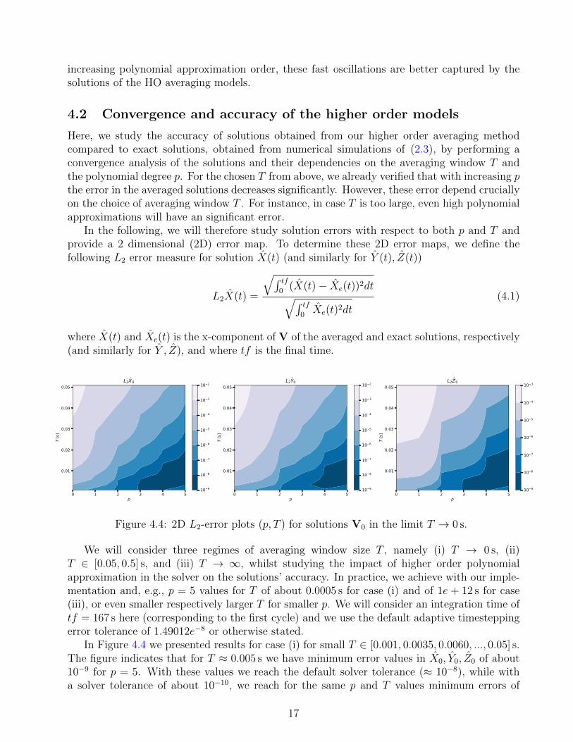
Figure 4.4: 2D L2-error plots (p, T ) for solutions V0 in the limit T → 0 s.

We will consider three regimes of averaging window size T , namely (i) T → 0 s, (ii)T ∈ [0.05, 0.5] s, and (iii) T → ∞, whilst studying the impact of higher order polynomialapproximation in the solver on the solutions’ accuracy. In practice, we achieve with our imple-mentation and, e.g., p = 5 values for T of about 0.0005 s for case (i) and of 1e + 12 s for case(iii), or even smaller respectively larger T for smaller p. We will consider an integration time oftf = 167 s here (corresponding to the first cycle) and we use the default adaptive timesteppingerror tolerance of 1.49012e−8 or otherwise stated.

In Figure 4.4 we presented results for case (i) for small T ∈ [0.001, 0.0035, 0.0060, ..., 0.05] s.The figure indicates that for T ≈ 0.005 s we have minimum error values in X0, Y0, Z0 of about10−9 for p = 5. With these values we reach the default solver tolerance (≈ 10−8), while witha solver tolerance of about 10−10, we reach for the same p and T values minimum errors of

17

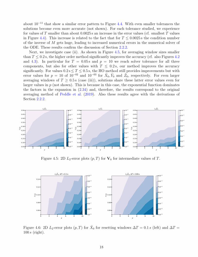
about 10−11 that show a similar error pattern to Figure 4.4. With even smaller tolerances thesolutions become even more accurate (not shown). For each tolerance studied, we experiencefor values of T smaller than about 0.0025 s an increase in the error values (cf. smallest T valuesin Figure 4.4). This increase is related to the fact that for T ≤ 0.0025 s the condition numberof the inverse of M gets huge, leading to increased numerical errors in the numerical solver ofthe ODE. These results confirm the discussion of Section 2.2.2.

Next, we investigate case (ii). As shown in Figure 4.5, for averaging window sizes smallerthan T ≤ 0.2 s, the higher order method significantly improves the accuracy (cf. also Figures 4.2and 4.3). In particular for T = 0.05 s and p = 10 we reach solver tolerance for all threecomponents, but also for other values with T ≤ 0.2 s, our method improves the accuracysignificantly. For values 0.2 s≤ T ≤ 0.5 s, the HO method still provides improvements but witherror values for p = 10 of 10−02 and 10−03 for X0, Y0 and Z0, respectively. For even largeraveraging windows of T ≥ 0.5 s (case (iii)), solutions share these latter error values even forlarger values in p (not shown). This is because in this case, the exponential function dominatesthe factors in the expansion in (2.34) and, therefore, the results correspond to the originalaveraging method of Peddle et al. (2019). Also these results agree with the derivations ofSection 2.2.2.

0 2 4 6 8 10p

0.05

0.10

0.15

0.20

0.25

0.30

0.35

0.40

0.45

0.50

T [s

]

L2X0

10 9

10 8

10 7

10 6

10 5

10 4

10 3

10 2

10 1

0 2 4 6 8 10p

0.05

0.10

0.15

0.20

0.25

0.30

0.35

0.40

0.45

0.50

T [s

]

L2Y0

10 9

10 8

10 7

10 6

10 5

10 4

10 3

10 2

10 1

0 2 4 6 8 10p

0.05

0.10

0.15

0.20

0.25

0.30

0.35

0.40

0.45

0.50

T [s

]

L2Z0

10 9

10 8

10 7

10 6

10 5

10 4

10 3

10 2

Figure 4.5: 2D L2-error plots (p, T ) for V0 for intermediate values of T .

0 2 4 6 8 10p

0.06

0.08

0.10

0.12

0.14

T [s

]

L2X0, T = 0.1 s

10 9

10 8

10 7

10 6

10 5

10 4

10 3

10 2

0 2 4 6 8 10p

0.06

0.08

0.10

0.12

0.14

T [s

]

L2X0, T = 100 s

10 9

10 8

10 7

10 6

10 5

10 4

10 3

10 2

Figure 4.6: 2D L2-error plots (p, T ) for X0 for resetting windows ∆T = 0.1 s (left) and ∆T =100 s (right).

18

As indicated above, the resetting after the time interval ∆T of the higher order velocitycomponents prevents the HO models from blowups. The latter are due to instabilities in thehigher order terms which, in turn, are caused by a growing discrepancy between principal andhigher order modes in V that might happen after long simulation times, cf. Figure 4.2. InFigure 4.6, we present error plots for X0 solutions obtained with the higher order averagingapproach for two different resetting values: ∆T = 0.1 s (left) and ∆T = 100 s (right). Thesimilarity of both error maps indicates that a change in the resetting window size ∆T has almostno impact on the accuracy of the solutions. This property is shared by the corresponding errormaps for the Y0 and Z0 components (not shown).

5 Summary and outlook

In this paper we introduced a higher order finite window averaging technique and investigated itby specialising to Gaussian weight functions to allow for explicit computation of averages. Thisenabled us to efficiently investigate the higher order technique when applied to highly oscillatoryODEs, in particular Lynch’s swinging spring model. We found that higher order corrections canstrongly increase the accuracy of the averaged model solutions, but only when the averagingwindow is close to the time period of the fast frequency (this model only has two fast frequencies,in 2:1 resonance). We expect the situation to become more complicated when there are aspectrum of fast frequencies. In this case, it is known that very high frequencies do not changethe slow components of the solution much, but moderate fast frequencies can resonate in thenonlinearity (just like in the swinging spring), altering the slow dynamics. In this case onewould want to select an averaging window that removes as much fast dynamics as possible,whilst preserving accuracy of the slow dynamics arising from near-resonant interactions, andthe higher order model could prove useful in reducing the impact of the averaging on this slowdynamics.

In this paper we have also avoided numerical aspects, such as the effects of approximateaverages by numerical quadrature, and the interaction of numerical time integratores with theaveraging. An analysis using the ideas of Peddle et al. (2019) would also be useful here. Lookingfurther ahead, if the higher order averaging model is shown to improve the accuracy of averagingmethods whilst still allowing larger time steps in numerical integrations, this would motivatethe investigation of multilevel schemes such as PFASST, where the low order averaging is usedas a coarse propagator and higher order averaging models provide higher order corrections,some of which can be hidden in parallel behind first iterations in later timesteps.

Acknowledgement

The authors would like to acknowledge funding from NERC NE/R008795/1 and from EPSRCEP/R029628/1.

A Fully explicit representation for p = 2

Here, we present a fully explicit version of (2.39) in terms of tendencies for V0, V1, andV2. Split into these tendencies while inserting values for Rm

α and taking into account that

19

Fm,j,k = Fm,k,j∀m, j, k, we arrive at

V0(t) =M∑m=1

eicmte−c2mT2

2

(3

2Fm,0,01 +

3

2Fm,1,1(T

2 − k2mT 4) +3

2Fm,2,2(3T

4 − 6k2mT6 + k4mT

8)

+ 3Fm,0,1(icmT2) + 3Fm,0,2(T

2 − k2mT 4) + 3Fm,1,2(i3kmT4 − ik3mT 6)

− 1

2Fm,0,0(1− k2mT 2)− 1

2Fm,1,1(3T

2 − 6k2mT4 + k4mT

6)

− 1

2Fm,2,2(15T 4 − 45k2mT

6 + 15k4mT8 − k6mT 10)− Fm,0,1(i3kmT

2 − ik3mT 4)

− Fm,0,2(3T2 − 6k2mT

4 + k4mT6)− Fm,1,2(i15kmT

4 − i10k3mT6 + ik5mT

8)),

which can be summarized to

V0(t) =M∑m=1

eicmte−c2mT2

2

(Fm,0,0(1 +

1

2c2mT

2) + Fm,1,1(3

2c2mT

4 − 1

2c4mT

6)

+ Fm,2,2(−3T 4 +27

2c2mT

6 − 6c4mT8 +

1

2c6mT

8)

+ Fm,0,1(ic3mT

4) + Fm,0,2(3c2mT

4 − c4mT 6) + Fm,1,2(−6icmT4 + 7ic3mT

6 − ic5mT 8)).

For V1, there follows directly

V1(t) =M∑m=1

eicmte−c2mT2

2

(Fm,0,0(icm) + Fm,1,1(i3cmT

2 − ic3mT 4) + Fm,2,2(i15cmT4 − i10c3mT

6 + ic5mT8)

+ 2Fm,0,1(1− c2mT 2) + 2Fm,0,2(i3cmT2 − ic3mT 4) + 2Fm,1,2(3T

2 − 6c2mT4 + c4mT

6)).

Finally for V2, we find

V2(t) =M∑m=1

eicmte−c2mT2

2

(− 1

2Fm,0,01/T

2 − 1

2Fm,1,1(T

0 − k2mT 2)− 1

2Fm,2,2(3T

2 − 6k2mT4 + k4mT

6)

− Fm,0,1(ikmT0)− Fm,0,2(T

0 − k2mT 2)− Fm,1,2(i3kmT2 − ik3mT 4)

+1

2Fm,0,0(1/T

2 − k2mT 0) +1

2Fm,1,1(3T

0 − 6k2mT2 + k4mT

4)

+1

2Fm,2,2(15T 2 − 45k2mT

4 + 15k4mT6 − k6mT 8)

+ Fm,0,1(i3kmT0 − ik3mT 2) + Fm,0,2(3T

0 − 6k2mT2 + k4mT

4)

+ Fm,1,2(i15kmT2 − i10k3mT

4 + ik5mT6)),

which leads to

V2(t) =M∑m=1

eicmte−c2mT2

2

(Fm,0,0(−

1

2c2m) + Fm,1,1(1−

5

2c2mT

2 +1

2c4mT

4)

+ Fm,2,2(6T2 − 39

2c2mT

4 + 7c4mT6 − 1

2c6mT

8)

+ Fm,0,1(2icm) + Fm,0,2(2− 5c2mT2 + c4mT

4) + Fm,1,2(12icmT2 − 9ic3mT

4 + ic5mT6)).

20

References

Abdulle, A., Weinan, E., Engquist, B., Vanden-Eijnden, E., 2012. The heterogeneous multiscalemethod. Acta Numerica 21, 1–87.

Babin, A., Mahalov, A., Nicolaenko, B., Zhou, Y., Jun 1997. On the asymptotic regimes andthe strongly stratified limit of rotating boussinesq equations. Theoretical and ComputationalFluid Dynamics 9 (3), 223–251.

Caliari, M., Einkemmer, L., Moriggl, A., Ostermann, A., 2021. An accurate and time-parallelrational exponential integrator for hyperbolic and oscillatory pdes. Journal of ComputationalPhysics 437, 110289.

Charney, J. G., Fjortoft, R., von Neumann, J., 1950. Numerical Integration of the BarotropicVorticity Equation. Tellus 2, 237–254.

Davies, T., Staniforth, A., Wood, N., Thuburn, J., 2003. Validity of anelastic and other equationsets as inferred from normal-mode analysis. Quarterly Journal of the Royal MeteorologicalSociety 129 (593), 2761–2775.

Haut, T., Wingate, B., 2014. An asymptotic parallel-in-time method for highly oscillatoryPDEs. SIAM Journal on Scientific Computing 36 (2), A693–A713.

Haut, T. S., Babb, T., Martinsson, P., Wingate, B., 2016. A high-order time-parallel schemefor solving wave propagation problems via the direct construction of an approximate time-evolution operator. IMA Journal of Numerical Analysis 36 (2), 688–716.

Holm, D. D., Lynch, P., 2002. Stepwise precession of the resonant swinging spring. SIAMJournal on Applied Dynamical Systems 1 (1), 44–64.

Jones, D., Mahalov, a., Nicolaenko, B., 1999. A Numerical Study of an Operator SplittingMethod for Rotating Flows with Large Ageostrophic Initial Data. Theoretical and Compu-tational Fluid Dynamics 13 (2), 143.URL http://link.springer.de/link/service/journals/00162/bibs/9013002/

90130143.htm

Majda, A. J., Embid, P., 1998. Averaging over fast gravity waves for geophysical flows withunbalanced initial data. Theoretical and computational fluid dynamics 11 (3-4), 155–169.

Minion, M., 2011. A hybrid parareal spectral deferred corrections method. Communications inApplied Mathematics and Computational Science 5 (2), 265–301.

Peddle, A. G., Haut, T., Wingate, B., 2019. Parareal convergence for oscillatory PDEs withfinite time-scale separation. SIAM Journal on Scientific Computing 41 (6), A3476–A3497.

Sanders, J. A., Verhulst, F., Murdock, J., 2007. Averaging methods in nonlinear dynamical sys-tems, 2nd Edition. Applied mathematical sciences. Springer, New York, Berlin, Heidelberg.

Schochet, S., 1994. Fast singular limits of hyperbolic pdes. Journal of differential equations114 (2), 476–512.

Schreiber, M., Peixoto, P. S., Haut, T., Wingate, B., 2018. Beyond spatial scalability limitationswith a massively parallel method for linear oscillatory problems. The International Journalof High Performance Computing Applications 32 (6), 913–933.

Smith, L. M., Waleffe, F., 2002. Generation of slow large scales in forced rotating stratifiedturbulence. Journal of Fluid Mechanics 451, 145–168.

Wingate, B. A., Embid, P., Holmes-Cerfon, M., Taylor, M. A., 2011. Low Rossby limitingdynamics for stably stratified flow with finite froude number. Journal of fluid mechanics 676,546–571.

21