Higher-dimensional SYK Non-Fermi Liquids at Lifshitz transitions

Arijit Haldar,∗ Sumilan Banerjee,† and Vijay B. Shenoy‡

Centre for Condensed Matter Theory, Department of Physics,Indian Institute of Science, Bangalore 560 012, India

(Dated: October 4, 2017)

We address the key open problem of a higher dimensional generalization of the Sachdev-Ye-Kitaev(SYK) model. We construct a model on a lattice of SYK dots with non-random intersite hopping.The crucial feature of the resulting band dispersion is the presence of a Lifshitz point where twobands touch with a tunable powerlaw divergent density of states (DOS). For a certain regime ofthe powerlaw exponent, we obtain a new class of interaction-dominated non-Fermi liquid (NFL)states, which exhibits exciting features such as a zero-temperature scaling symmetry, an emergent(approximate) time reparameterization invariance, a powerlaw entropy-temperature relationship,and a fermion dimension that depends continuously on the DOS exponent. Notably, we furtherdemonstrate that these NFL states are fast scramblers with a Lyapunov exponent λL ∝ T , althoughthey do not saturate the upper bound of chaos, rendering them truly unique.

Description of quantum many-body systems lackingqausiparticle excitations [1] is a longstanding and chal-lenging problem at the forefront of physics research to-day. A solvable instance of such a system in 0-dimensionis provided by the SYK model [2, 3], which has attracteda lot of attention recently due to its intriguing connec-tions to quantum gravity in AdS2 [3–7] and intertwinedquestions of thermalization and information scrambling.The exciting possibility of generalizing this model tohigher dimensions to address questions relating to trans-port without quasiparticles as well as to look for possibledual to higher-dimensional gravity, has lead to a numberof interesting extensions [8–15] of SYK model.

The attempts to generalize SYK model to higher di-mensions typically use a lattice of SYK dots, connectedvia either random interdot interaction and/or hopping[8–11, 15] or through uniform hopping leading to a trans-lationally invariant system [16]. These generalizationshave lead to extraction of transport quantities and diag-nostics of many-body quantum chaos, such as the but-terfly velocity [8], in strongly interacting lattice models,demonstrating their connection, e.g., with the phenom-ena like heavy-Fermi liquids [11] and many-body local-ization [9]. However, such extensions have met with onlypartial success towards a ‘canonical’ higher-dimensionalgeneralization. In particular, the ensuing low-energy be-havior turns out to be either qualitatively similar to thatof the 0-dimensional SYK model at the leading order [8],or results in a low-temperature phase where interactionbecomes irrelevant [11, 16] at low energies. A notablehigher-dimensional extension of SYK model by Berkoozet al. [12] has succeeded in obtaining an interaction-dominated fixed point distinct from 0-dimensional modelby allowing SYK interactions only to low momentumfermions by using a phenomenological ‘filter function’construct whose microscopic underpinnings are unclear.Such issues have left the higher-dimensional extension ofthe SYK model as an interesting open problem. Here wepropose and extensively study a microscopically moti-vated, translationally invariant lattice model, exhibitinga new class of interaction-dominated non-Fermi liquid

(NFL) fixed points, derived from the SYK model.

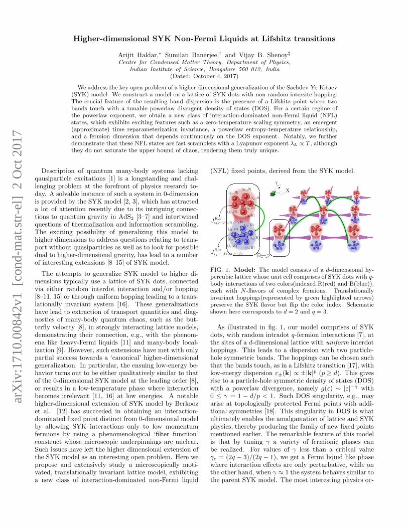
FIG. 1. Model: The model consists of a d-dimensional hy-percubic lattice whose unit cell comprises of SYK dots with q-body interactions of two colors(indexed R(red) and B(blue)),each with N -flavors of complex fermions. Translationallyinvariant hoppings(represented by green highlighted arrows)preserve the SYK flavor but flip the color index. Schematicshown here corresponds to d = 2 and q = 3.

As illustrated in fig. 1, our model comprises of SYKdots, with random intradot q-fermion interactions [7], atthe sites of a d-dimensional lattice with uniform interdothoppings. This leads to a dispersion with two particle-hole symmetric bands. The hoppings can be chosen suchthat the bands touch, as in a Lifshitz transition [17], withlow-energy dispersion ε±(k) ∝ ±|k|p (p ≥ d). This givesrise to a particle-hole symmetric density of states (DOS)with a powerlaw divergence, namely g(ε) ∼ |ε|−γ with0 ≤ γ = 1 − d/p < 1. Such DOS singularity, e.g., mayarise at topologically protected Fermi points with addi-tional symmetries [18]. This singularity in DOS is whatultimately enables the amalgamation of lattice and SYKphysics, thereby producing the family of new fixed pointsmentioned earlier. The remarkable feature of this modelis that by tuning γ a variety of fermionic phases canbe realized. For values of γ less than a critical valueγc = (2q − 3)/(2q − 1), we get a Fermi liquid like phasewhere interaction effects are only perturbative, while onthe other hand, when γ ≈ 1 the system behaves similar tothe parent SYK model. The most interesting physics oc-

arX

iv:1

710.

0084

2v1

[co

nd-m

at.s

tr-e

l] 2

Oct

201

7

2

cur for γc < γ < 1, where the emergent NFL phases cor-respond to a new set of fixed points with a continuouslytunable fermion dimension ∆ = (1 + γ)/2(1 − γ + 2γq).As a result, the NFL phases have properties tunable viaγ, and distinct from that of the parent SYK model. Wefind that unlike the pure SYK phase, the NFL phaseshave zero ground-state entropy (S(T = 0)), with S(T )varying as a powerlaw in T with γ dependent exponent.Moreover, the onset of quantum chaos in the model isgoverned by a Lyapunov exponent λL ∝ T , which, how-ever, does not saturate the chaos bound of λL = 2πT[3, 19]. As γ → 1, the residual zero-temperature entropyof the parent SYK is recovered and λL → 2πT .

The truly higher-dimensional nature of the model ismanifested in the non-trivial dynamical scaling exponentz of the fermions. The perturbative fixed point (γ < γc)retains z = p of the non-interacting model. Whereas,for γ > γc, interaction changes the dynamical exponentfrom z = p to z = p/(2(2q − 1)∆− 1), not unlike a pro-posed quantum gravity theory [20] which exploits Lif-shitz points. Thus our work offers a solution to themuch sought after higher-dimensional generalization ofthe SYK model and provides a framework for address-ing problems ranging from the nature of transport andthermalization in systems without quasiparticles to pos-sible realizations of higher-dimensional duals of quantumgravity models.

Model: Our lattice model (fig. 1 ) is described by thefollowing Hamiltonian

H =−∑

x,x′,α,α′

tαα′(x− x′)c†iαxciα′x′ − µ∑x,iα

c†iαxciαx

+∑x,α

∑i1,··· ,iq,j1,··· ,jq

Jα,xi1,··· ,iq ;j1,··· ,jqc†iqαx· · · c†i1αxcj1αx · · · cjqαx,

(1)

where i, j = 1, · · · , N denote SYK flavor at the latticepoint x in d dimension and α, α′ = R(red), B(blue)index the two colors for the fermion operators c, c†.The intradot complex random all-to-all q-body SYKcouplings Jα,xi1,··· ,iq ;j1,··· ,jq are completely local and scatter

fermions having the same color index (see fig. 1). Theseamplitudes are identically distributed independentrandom variables with variance J2/qN2q−1(q!)2,

such that 〈Jα,xi1,···,iq ;j1,···,jqJα,x′

i′1,···,i′qc ;j′1,···,j′qc〉 ∝

δα,α′δx,x′q∏a=1

δia,i′aδja,j′a , where i1(i′1) < · · · < iq(i′q)

and j1(j′1) < · · · < jq(j′q). Hopping from one lattice

point to another, that always flips the color index, isfacilitated by tαβ(x − x′) that conserves the SYK flavorof the fermion. By tuning the magnitude and range ofthese hoppings, a low-energy dispersion ε±(k) of theform,

ε±(k) ∝ ±|k|p, (2)

can be generated. We choose p ≥ d to be an integer

to obtain a particle-hole symmetric DOS, with an inte-grable powerlaw singularity, of the form g(ε) ∼ |ε|−γ ,where γ = 1 − d/p. Evidently, γ can be varied between0 to 1 by tuning p and d. Such dispersions with a low-energy form given by eqn. (2) can be easily ‘designed’ fora d-dimensional lattice (see the Supplementary Material(SM), SM S1 for details [21]), e.g., a lattice dispersion ind = 1 corresponding to eqn. (2) is ε±(k) ∝ ±| sin(k/2)|p,with k in units of inverse lattice spacing. The low-energydispersion in eqn. (2) implies the following approximateform for the single-particle DOS

g(ε) = g0|ε|−γΘ(Λ− |ε|) (3)

where Θ denotes Heaviside step function and Λ > 0, aenergy cutoff, that plays the role of the bandwidth. Theconstant g0 = (1− γ)/(2Λ1−γ) normalizes the integratedDOS to unity. The above low-energy form of the DOS issufficient to study the low-temperature properties of themodel of eqn. (1) for Λ, J T .

Saddle-point equations: The model of eqn. (1) is solv-able at the level of saddle point, which becomes exact inthe limit N → ∞, i.e., when the SYK dots consist ofa large number of SYK flavors. To derive the saddlepoint equations [5, 8] we disorder average over the ran-dom SYK couplings using replicas and obtain an effectiveaction within a replica-diagonal ansatz in terms of large-N collective field

Gαx(τ1, τ2) =1

N

∑i

〈ciαx(τ1)c†iαx(τ2)〉, (4)

and its conjugate Σαx(τ1, τ2), where τ1,2 denote imagi-nary time (see SM S2). Further, retaining color sym-metry and lattice translational invariance for the saddle-point, we obtain the following action (per site, per SYKflavor)

S =−∫

dτ1,2∫

dεg(ε)Tr ln [(∂τ1 + ε)δ(τ1 − τ2) + Σ(τ1, τ2)]

−∫

dτ1,2

[(−1)q J

2

2qGq(τ1, τ2)Gq(τ2, τ1)

+Σ(τ2, τ1)G(τ1, τ2)] , (5)

where∫dτ1,2 =

∫dτ1dτ2. The above action leads to self-

consistent equations for the collective fields G and Σ,

G(iωn) =

∫ Λ

−Λ

dεg(ε) [iωn − ε− Σ(iωn)]−1

(6a)

Σ(τ) =(−1)q+1J2Gq(τ)Gq−1(−τ), (6b)

where ωn = 2πnT is the fermionic Matsubara frequency,T is the temperature with i =

√−1, and we have assumed

time translation invariance, i.e., G(τ1, τ2) = G(τ1 − τ2).At the saddle point, G(τ) is the on-site fermion Green’sfunction and Σ(τ) is the self-energy, which is completelylocal in this model. The Green’s function of the fermionwith momentum k is given by

G±(k, iωn) = (iωn − ε±(k)− Σ(iωn))−1. (7)

3

Zero-temperature solutions: The low-energy solutionof the saddle-point equations (6) can be obtained ana-lytically at T = 0. At low temperatures, in the limitω, Σ(ω) Λ, we expand the integral for G(iωn →ω + i0+) in eqn. (6a) in powers of (ω − Σ(ω))/Λ to get

G(ω) ≈g0π(1− eiγπ)

sin(πγ) (ω − Σ(ω))γ (8)

at the leading order. As we show below, the above equa-tions leads to two possible fixed point solutions – (1) anew interaction-dominated fixed point for ω Σ(ω) asω → 0 and (2) the original lattice-dominated fixed pointfor ω Σ(ω), essentially a ‘Fermi liquid’, where interac-tion becomes irrelevant for ω → 0.

In the first case, eqn. (8) becomes

G(ω) = g0(1− eiγπ)π csc(πγ)Σ(ω)−γ . (9)

At zero temperature, the self-consistent solution ofeqns.(6b),(9) is obtained by taking a powerlaw ansatzfor G(ω), as in the conventional SYK model [2, 5]. Thisleads to

G(ω) =Ce−iθω2∆−1 (10a)

Σ(ω) =J2 (CΓ(2∆) sin θ)

2q−1

Γ(2∆Σ) sin(π∆Σ)π2q−1eiπ∆Σω2∆Σ−1 (10b)

where the fermion scaling dimension ∆ and the prefactorC are determined self-consistently to be(see SM S3 fordetails)

∆ =1 + γ

2(1− γ + 2qγ)(11)

C =

[g0π

2γ(q−1)+1

J2γ cos(γπ/2)

(Γ(2∆Σ) sin (π∆Σ)

(Γ(2∆) sin(π∆))2q−1

)γ] 2∆1+γ

with ∆Σ = (2q − 1)∆, and Γ(x) is the gamma func-tion. The low-energy saddle-point equations, and theconstraint ImG(ω) < 0, completely fix the spectral asym-metry parameter θ to π∆ in our case, allowing onlyparticle-hole symmetric scaling solutions at the interact-ing fixed point, which should be contrasted with the usualSYK model where θ can be tuned by filling.

The fact that the fermion dimension ∆ is determinedboth by the lattice DOS via γ and by SYK interac-tions through q, indicates that the fixed point is in-deed a ‘truly’ higher-dimensional analogue of the 0-dimensional SYK phase, but yet distinct from it. Infact as γ → 1, ∆ → 1/2q and the fermion dimensionof the 0-dimensional SYK model is recovered. How-ever, unlike the SYK model which has an asymptoticallyexact infrared time reparametrization symmetry underτ → f(τ), eqn. (6)(b) together with eqn. (9) are invari-ant only under time translation and scaling transforma-tions, τ → aτ + b; a, b being constants. One wouldexpect time reparametrization symmetry to be restored

as the 0-dimensional SYK-like fixed point at γ → 1 isapproached.

The dependence of ∆ on γ(eqn. (11)) also implies thatin principle ∆ can be changed continuously starting from1/2q to 1/2, as γ is tuned from 1 to 0. However, asevident from eqn. (10b), the assumption ω Σ(ω), isonly self consistent as long as 2∆Σ − 1 ≥ 1, i.e.

1 ≥ γ ≥ 2q − 3

2q − 1≡ γc(q). (12)

Therefore, below a q-dependent critical value γc(q) thescaling solution (10a) ceases to exist. This brings us tothe saddle-point solution for the perturbative fixed pointfor ω Σ(ω), henceforth referred to as lattice-Fermiliquid (LFL). In this limit, eqn. (8) reduces to

G(ω) ≈g0(1− eiγπ)π csc(πγ)(ω)−γ . (13)

It can be shown that at this fixed-point Σ(ω) ∼(J2/Λ)(ω/Λ)(1−γ)(2q−1)−1 ω for γ < γc, i.e., inter-action is irrelevant and its effect is only perturbative inJ for ω → 0. The dominant term in the Green’s func-tion above is determined only by the singularity in thesingle-particle DOS and is temperature independent. Atfinite temperatures there are small corrections of O(J2).We use this fact in the next section to numerically verifythe existence of the LFL.

In gist, we find that the system undergoes a quantumphase transition at γ = γc(q) upon increasing γ from0 to 1. For γ < γc, we have a LFL, while for γ > γcwe get a line of interaction dominated NFLs. This isalso indicated by the dynamical exponent, deduced fromeqn. (7), that changes from z = p(when γ < γc) to z =p/(2∆Σ − 1)(when γ > γc) across γc.

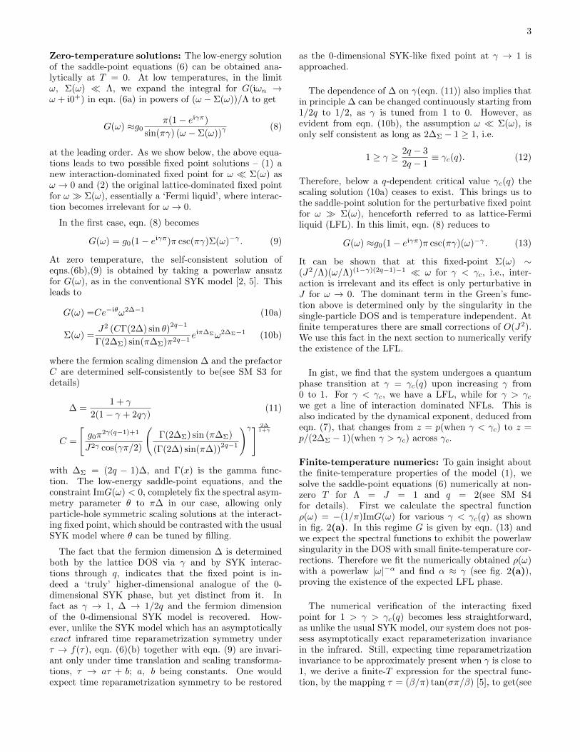
Finite-temperature numerics: To gain insight aboutthe finite-temperature properties of the model (1), wesolve the saddle-point equations (6) numerically at non-zero T for Λ = J = 1 and q = 2(see SM S4for details). First we calculate the spectral functionρ(ω) = −(1/π)ImG(ω) for various γ < γc(q) as shownin fig. 2(a). In this regime G is given by eqn. (13) andwe expect the spectral functions to exhibit the powerlawsingularity in the DOS with small finite-temperature cor-rections. Therefore we fit the numerically obtained ρ(ω)with a powerlaw |ω|−α and find α ≈ γ (see fig. 2(a)),proving the existence of the expected LFL phase.

The numerical verification of the interacting fixedpoint for 1 > γ > γc(q) becomes less straightforward,as unlike the usual SYK model, our system does not pos-sess asymptotically exact reparameterization invariancein the infrared. Still, expecting time reparametrizationinvariance to be approximately present when γ is close to1, we derive a finite-T expression for the spectral func-tion, by the mapping τ = (β/π) tan(σπ/β) [5], to get(see

4

ρ(ω

)

ω

(a)γ=0.1 α=0.097γ=0.3 α=0.28

-0.04 0 0.04ω

(b)γ=0.5γ=0.7γ=0.9

-0.04 0 0.04

0.01

0.1

1

0.001 0.01 0.1

S

T

(c) γ = 0.1γ = 0.2γ = 0.3γ = 0.4γ = 0.5γ = 0.6γ = 0.7γ = 0.8γ = 0.9

ζ

γ

num.1− γ(2∆Σ − 1)(1 − γ)

0

0.2

0.4

0.6

0.8

1

0 0.2 0.4 0.6 0.8 1

(d)

LFLNFL

γc

FIG. 2. Numerical results (q = 2, J = Λ = 1): (a)Spectral function at T = 5× 10−3 from numerics(points) fit-ted with the powerlaw |ω|−α(solid lines), where α = 0.097 ±0.0003, 0.28 ± 0.0006 for γ = 0.1, 0.3 respectively. (b) Nu-merical spectral function(points) at T = 5 × 10−3 for γ =0.5, 0.7, 0.9 compared, with no fitting parameters, to thoseobtained analytically(solid lines) using reparametrization in-variance(eqn. (14)). (c)Entropy(S) vs. temperature(T ) forvarious γ shown in log-log scale, demonstrating the power-law dependence of S on T . (d)The temperature exponent(ζ)for S(points) as a function of γ, compared with theoreti-cal predictions(lines) in the lattice-Fermi liquid(γ < γc(=1/3))(eqn. (16)) and non-Fermi liquid(γ > γc)(eqn. (15)) re-gions.

SM S5),

ρ(ω) =C sin(π∆) cosh (βω/2)

π2 (2π/β)2∆−1

Γ

(∆− i

βω

2π

)Γ

(∆ + i

βω

2π

),

(14)

where β = T−1. We compare the above with the ρ(ω) ob-tained numerically, anticipating only a qualitative match.Surprisingly, we find an excellent quantitative agreementbetween the two without using any fitting parameter, asdemonstrated in fig. 2(b). Moreover, eqn. (14) accu-rately matches the numerical result even for values of γfar away from 1 (see fig. 2(b)). This not only confirmsthe existence of NFL fixed points (see eqn. (10a)) butalso points to an approximate emergent reparametriza-tion symmetry at these fixed-points.

In order to verify this result further, we estimate finite-temperature entropy S(T ) using ρ(ω) from eqn. (14)and a similar finite-temperature form for the self-energyΣ(ω), both of which satisfy a scaling relation, e.g.,ρ(ω) ∼ (T/J)2∆−1f(ω/T ). We obtain the entropy viaS = −∂F/∂T , where the free-energy F is obtained byevaluating the action of eqn. (5) with the scaling formfor ρ(ω) and Σ(ω)(see SM S6 for details, and also [22]).We find that the low-temperature entropy vanishes with

0

0.2

0.4

0.6

0.8

1

0 0.1 0.2 0.3 0.4 0.5 0.6 0.7 0.8 0.9 1

λ(M

)

L/2πT

T

(a) γ = 0.1γ = 0.3γ = 0.4γ = 0.5γ = 0.6γ = 0.7γ = 0.8γ = 0.9γ = 0.95SYK

0.04

0.2

1

0.01 0.1 1 10

T

(b)

γ = 0.1γ = 0.3γ = 0.4γ = 0.5γ = 0.6γ = 0.7γ = 0.8γ = 0.9γ = 0.95SYK

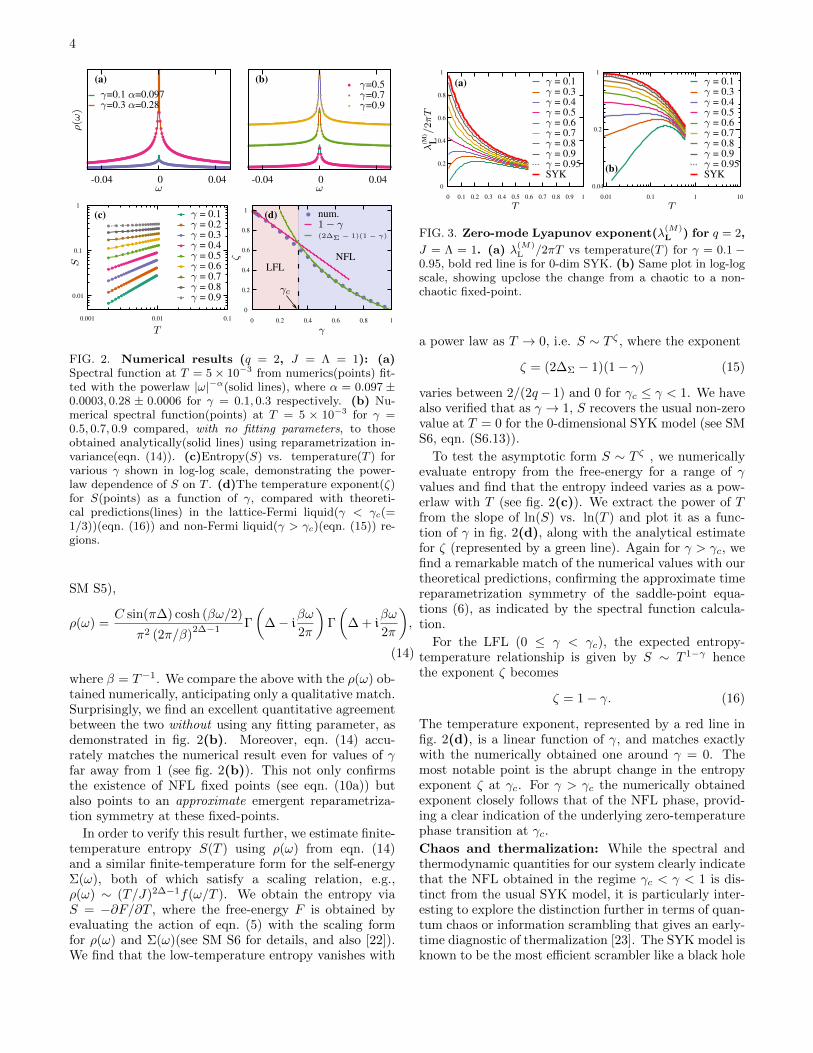
FIG. 3. Zero-mode Lyapunov exponent(λ(M)L ) for q = 2,

J = Λ = 1. (a) λ(M)L /2πT vs temperature(T ) for γ = 0.1 −

0.95, bold red line is for 0-dim SYK. (b) Same plot in log-logscale, showing upclose the change from a chaotic to a non-chaotic fixed-point.

a power law as T → 0, i.e. S ∼ T ζ , where the exponent

ζ = (2∆Σ − 1)(1− γ) (15)

varies between 2/(2q− 1) and 0 for γc ≤ γ < 1. We havealso verified that as γ → 1, S recovers the usual non-zerovalue at T = 0 for the 0-dimensional SYK model (see SMS6, eqn. (S6.13)).

To test the asymptotic form S ∼ T ζ , we numericallyevaluate entropy from the free-energy for a range of γvalues and find that the entropy indeed varies as a pow-erlaw with T (see fig. 2(c)). We extract the power of Tfrom the slope of ln(S) vs. ln(T ) and plot it as a func-tion of γ in fig. 2(d), along with the analytical estimatefor ζ (represented by a green line). Again for γ > γc, wefind a remarkable match of the numerical values with ourtheoretical predictions, confirming the approximate timereparametrization symmetry of the saddle-point equa-tions (6), as indicated by the spectral function calcula-tion.

For the LFL (0 ≤ γ < γc), the expected entropy-temperature relationship is given by S ∼ T 1−γ hencethe exponent ζ becomes

ζ = 1− γ. (16)

The temperature exponent, represented by a red line infig. 2(d), is a linear function of γ, and matches exactlywith the numerically obtained one around γ = 0. Themost notable point is the abrupt change in the entropyexponent ζ at γc. For γ > γc the numerically obtainedexponent closely follows that of the NFL phase, provid-ing a clear indication of the underlying zero-temperaturephase transition at γc.

Chaos and thermalization: While the spectral andthermodynamic quantities for our system clearly indicatethat the NFL obtained in the regime γc < γ < 1 is dis-tinct from the usual SYK model, it is particularly inter-esting to explore the distinction further in terms of quan-tum chaos or information scrambling that gives an early-time diagnostic of thermalization [23]. The SYK model isknown to be the most efficient scrambler like a black hole

5

[3], namely the Lyapunov exponent λL, characterizingdecay of a typical out-of-time-ordered (OTO) correlator,

e.g., 〈c†i (t)c†j(0)ci(t)cj(0)〉 ' f0− (f1/N)eλLt +O

(N−2

),

saturates the upper bound, λL = 2πT , imposed by quan-tum mechanics [19, 24]. A natural question is then to ask,whether our new NFL states behave similarly or differ-ently. To this end, we generalize the OTO correlator forour two-band lattice system as

1

N2

∑ij

〈c†iαx(t)c†jβx′(0)ciαx(t)cjβx′(0)〉

1

N2

∑ij

〈ciαx(t)c†jβx′(0)c†iαx(t)cjβx′(0)〉

and find that their time evolution is governed by twolattice-momentum (q) dependent modes, an intrabandmode and an interband one. At q = 0 the lattice dis-persion enters into the expressions of OTO correlator forboth the modes only through the overall DOS g(ε) (seeSM S7, eqn. (S7.24)). Also at q = 0 the intraband mode

has the larger Lyapunov exponent (λ(M)L ) among the two

and therefore dominates the onset of chaos (see SM S7).

We numerically calculate λ(M)L for q = 2 as a function

of T for various values of γ on both sides of the quantumcritical point γc(q = 2) = 1/3 as show in fig. 3. We

find that λ(M)L /2πT becomes identical with that of 0-

dimensional SYK model (represented by a bold red line

in fig. 3(a)) as γ → 1. In particular λ(M)L /2πT → 1 as

T → 0, thereby saturating the chaos bound.

For γc < γ < 1, our numerical results indicate in the

limit T → 0, λ(M)L /2πT → α, where 0 < α < 1. This dis-

tinct behavior from original SYK model implies that the

NFL fixed points here do not saturate the chaos boundalthough they are still very efficient scramblers with Lya-punov exponent ∝ T at low temperature. Interestinglysimilar behavior has been reported [25], in systems, albeitin a less controlled calculation, involving fermions cou-pled to a gauge field. Around the neighborhood of γc forγ = (0.3−0.5), α starts to turn around and tend towardszero (see fig. 3(b)), signifying a change in the chaotic be-

havior of the system. Finally, for γ < γc, λ(M)L /2πT → 0

as T → 0 indicating the presence of a slow scramblingphase similar to a Fermi-liquid.Discussion: In this paper, we have developed a modelthat achieves a higher-dimensional generalization of theSYK model. The class of NFL phases discovered hereshould provide a platform to study transport propertiesin strongly interacting quasiparticle-less lattice systems,with non-random hoping amplitudes. The latter allowsto go beyond purely diffusive transport [8–11] and studythe interplay of fermion dispersion and interaction inNFL phases, in a manner not possible prior to this work.To this end, it would be interesting to explore connec-tion between transport and scrambling in our model [26]and contrast with that in other lattice generalizationsof SYK model with random hoppings [8]. This workalso has relevance towards the study of interaction ef-fects near Lifshitz transitions – a question that is relevantfrom the perspective of transitions between band insulat-ing topological phases that are generically separated bysuch transitions. Finally, it would be interesting to un-derstand how does approximate time reparametrizationsymmetry emerges in our system and what implicationsdoes it have from the point of view of the gravitationaldual.Acknowledgements: The authors AH and VBS thankDST, India for support.

∗ arijithaldar@iisc.ac.in† sumilan@iisc.ac.in‡ shenoy@iisc.ac.in

[1] S. Sachdev, Quantum Phase Transitions, 2nd ed. (Cam-bridge University Press, 2011).

[2] S. Sachdev and J. Ye, Phys. Rev. Lett. 70, 3339 (1993).[3] A. Kitaev, Talks at KITP, April 7, 2015 and May 27,

2015 .[4] S. Sachdev, Phys. Rev. Lett. 105, 151602 (2010).[5] S. Sachdev, Physical Review X 5, 1 (2015), 1506.05111.[6] J. Polchinski and V. Rosenhaus, Journal of High Energy

Physics 2016, 1 (2016).[7] J. Maldacena and D. Stanford, Phys. Rev. D 94, 106002

(2016).[8] Y. Gu, X.-L. Qi, and D. Stanford, Journal of High En-

ergy Physics 2017, 125 (2017).[9] S.-K. Jian and H. Yao, (2017), arXiv:1703.02051 [cond-

mat.str-el].[10] C.-M. Jian, Z. Bi, and C. Xu, Phys. Rev. B96, 115122

(2017), arXiv:1703.07793 [cond-mat.str-el].[11] X.-Y. Song, C.-M. Jian, and L. Balents, (2017),

arXiv:1705.00117 [cond-mat.str-el].[12] M. Berkooz, P. Narayan, M. Rozali, and J. Simon,

(2016), arXiv:1610.02422 [hep-th].[13] R. A. Davison, W. Fu, A. Georges, Y. Gu, K. Jensen,

and S. Sachdev, Phys. Rev. B 95, 155131 (2017).[14] J. Murugan, D. Stanford, and E. Witten, JHEP 08, 146

(2017), arXiv:1706.05362 [hep-th].[15] S.-K. Jian, Z.-Y. Xian, and H. Yao, (2017),

arXiv:1709.02810 [hep-th].[16] P. Zhang, (2017), arXiv:1707.09589 [cond-mat.str-el].[17] I. M. Lifshitz, Sov. Phys. JETP 95, 1130 (1930).[18] T. T. Heikkila and G. E. Volovik, JETP Letters 92, 681

(2010).[19] J. Maldacena, S. H. Shenker, and D. Stanford, Journal

of High Energy Physics 2016, 1 (2016).[20] P. Horava, Phys. Rev. D 79, 084008 (2009).[21] See Supplemental Material.[22] O. Parcollet, A. Georges, G. Kotliar, and A. Sengupta,

Phys. Rev. B 58, 3794 (1998).[23] Y. Gu, A. Lucas, and X.-L. Qi, (2017), arXiv:1708.00871

[hep-th].

6

[24] S. Banerjee and E. Altman, Phys. Rev. B 95, 134302(2017).

[25] A. A. Patel and S. Sachdev, Proc. Nat. Acad. Sci. 114,1844 (2017), arXiv:1611.00003 [cond-mat.str-el].

[26] A. Haldar, S. Banerjee, and V. Shenoy, Manuscript un-der preparation (2017).

1

Supplemental Materialfor

Higher-dimensional SYK Non-Fermi Liquids at Lifshitz transitionsby Arijit Haldar, Sumilan Banerjee and Vijay B. Shenoy

S1: Lattice-models and dispersions

In this section we outline a procedure to obtain lattice dispersions with the low-energy form given by

ε(k) = ±|k|p, (S1.1)

where k = k1, · · · , kd is a d−dimensional vector in the Brillouin zone. These kind of particle-hole symmetricdispersions can be obtained from Hamiltonians with the following form∑

k

H(k) =∑k

[c†R(k) c†B(k)

] [ 0 t(k)t(k)∗ 0

] [cR(k)cB(k)

], (S1.2)

where R/B denotes the fermion color indices red/blue and t(k) is a function of lattice-momentum k obtained by aFourier transform of the hopping-amplitudes tr which are yet to be determined, such that

t(k) =∑r

−tre−ir·k, (S1.3)

The hopping tr is the amplitude for a red color fermion to hop to a site separated by r and flip its color to blue. Theresulting two-band (±) energy dispersion is given by

ε±(k) = ±√t(k)t(k)∗. (S1.4)

A natural candidate for the dispersion whose low energy form is given by eqn. (S1.1) would be

ε±(k) =

(d∑i=1

sin(ki/2)2

)p/2(S1.5)

since near k = 0 we have

(d∑i=1

sin(ki/2)2

)p/2≈(

d∑i=1

(ki/2)2

)p/2∝ ±|k|p. We choose ki/2 instead of ki since we

want the dispersions to be gapless only at k = 0. The problem of finding a suitable t(k) then reduces to factorizingthe following equation

t(k)t(k)∗ =

(d∑i=1

sin(ki/2)2

)p. (S1.6)

When p is an even integer we can factorize the RHS of the above equation by taking

t(k) =

(d∑i=1

sin(ki/2)2

)p/2. (S1.7)

Then by substituting sin(ki/2) = (eiki/2 − e−iki/2)/2i and expanding the resulting expression we can easily read offthe hopping amplitudes from the coefficients in the expansion. For e.g. for dimension d = 1 and p = 2 we get

t(k) = sin(k/2)2 =1

2− 1

4eik − 1

4e−ik, (S1.8)

implying a hopping configuration which is shown in fig. 4(a). Lattices constructed in this way will generically haveinversion (x → −x) and color interchange (R ↔ B) symmetries. When p is an odd integer the function t(k) that

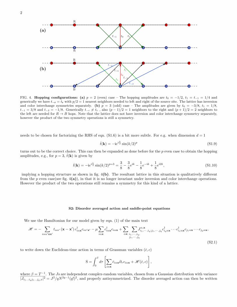
2

(a)

(b)

FIG. 4. Hopping configurations: (a) p = 2 (even) case – The hopping amplitudes are t0 = −1/2, t1 = t−1 = 1/4 andgenerically we have t−r = tr with p/2 = 1 nearest neighbors needed to left and right of the source site. The lattice has inversionand color interchange symmetries separately. (b) p = 3 (odd) case – The amplitudes are given by t0 = −3/8, t1 = 1/8,t−1 = 3/8 and t−2 = −1/8. Generically t−r 6= tr , also (p − 1)/2 = 1 neighbors to the right and (p + 1)/2 = 2 neighbors tothe left are needed for R→ B hops. Note that the lattice does not have inversion and color interchange symmetry separately,however the product of the two symmetry operations is still a symmetry.

needs to be chosen for factorizing the RHS of eqn. (S1.6) is a bit more subtle. For e.g. when dimension d = 1

t(k) = −iei k2 sin(k/2)p (S1.9)

turns out to be the correct choice. This can then be expanded as done before for the p even case to obtain the hoppingamplitudes, e.g., for p = 3, t(k) is given by

t(k) = −iei k2 sin(k/2)p=3 =3

8− 3

8eik − 1

8e−ik +

1

8ei2k, (S1.10)

implying a hopping structure as shown in fig. 4(b). The resultant lattice in this situation is qualitatively differentfrom the p even case(see fig. 4(a)), in that it is no longer invariant under inversion and color interchange operations.However the product of the two operations still remains a symmetry for this kind of a lattice.

S2: Disorder averaged action and saddle-point equations

We use the Hamiltonian for our model given by eqn. (1) of the main text

H = −∑

iαα′xx′

tαα′ (x− x′) c†iαxciα′x′ − µ∑iαx

c†iαxciαx +∑αx

∑i1,··· ,iq,j1,··· ,jq

Jα,xi1,··· ,iq ;j1,··· ,jqc†iqαx· · · c†i1αxcj1αx · · · cjqαx,

(S2.1)

to write down the Euclidean-time action in terms of Grassman variables (c, c)

S =

∫ β

0

dτ

[∑iαx

ciαx∂τ ciαx + H (c, c)

],

where β = T−1. The Js are independent complex-random variables, chosen from a Gaussian distribution with variance|Ji1...iqj1...jq,x|2 = J2/qN2q−1(q!)2, and properly antisymmetrized. The disorder averaged action can then be written

3

down using the replica-trick as

S =

∫dτ1

∫dτ2

∑ixx′αα′,r1

ciαxr1(τ1) [(∂τ1 − µ)δαα′δxx′ + tαα′ (x− x′)] δ(τ1 − τ2)ciα′x′r1(τ2)

−(−1)qJ2

2qN2q−1

∑αxr1r2

∑ij

ciαxr1(τ1)ciαxr2(τ2)ciαxr2(τ2)ciαxr1(τ1)

q (S2.2)

where r1, r2 are the replica indices. We introduce the large-N field Gαxr1r2(τ1, τ2) = 1N

∑i

ciαxr2(τ2)ciαxr1(τ1) and

the Lagrange multiplier Σαxr1r2(τ1, τ2) to obtain

S =

∫dτ1

∫dτ2

∑ixx′αα′,r1

ciαxr1(τ1) [(∂τ1 − µ)δαα′δxx′ + tαα′ (x− x′)] δ(τ1 − τ2)ciα′x′r1(τ2)

−N∑

αxr1r2

[(−1)q

J2

2qGqαxr1r2(τ1, τ2)Gqαxr2r1(τ2, τ1) +Gαxr1r2(τ1, τ2)Σαxr2r1(τ2, τ1)

]]. (S2.3)

The kinetic part of the action can be diagonalized by transforming the real space fermions ciαxr1(τ) to Bloch fermions,dibkr1(τ) , where b denotes the band index and takes the value +(−) for the upper(lower) band. Next we imposelattice translational and fermion color interchange invariance, such that Σαx = Σ and Gαx = G, then set µ = 0 anduse the replica-diagonal ansatz to obtain

S ≡ S

NNL=

1

NL

∫dτ1

∫dτ2

∑b=±,k

dibk(τ1) [(∂τ1 + εb,k)δ(τ1 − τ2) + Σ(τ1, τ2)] dibk(τ2)

−(−1)qJ2

2qGq(τ1, τ2)Gq(τ2, τ1)− Σ(τ2, τ1)G(τ1, τ2)

], (S2.4)

where NL is twice the total number of lattice sites, including the two colors and εb,k is the band dispersion. Tracingover the fermionic degrees of freedom we get

S =

∫dτ1

∫dτ2

−∑α,k

Tr ln [(∂τ1 + εb,k)δ(τ1 − τ2) + Σ(τ1, τ2)]− (−1)qJ2

2qGq(τ1, τ2)Gq(τ2, τ1)− Σ(τ2, τ1)G(τ1, τ2)

(S2.5)

By extremizing the action S, we obtain the saddle-point equations for G and Σ as

Σ(τ1, τ2) =(−1)q+1J2Gq−1(τ2, τ1)Gq(τ1, τ2) (S2.6a)

G(τ1, τ2) =〈cx(τ2)cx(τ1)〉 =1

NL

∑b,k

Gbk(τ1, τ2) (S2.6b)

where

G−1bk (τ1, τ2) = − [(∂τ1 + εb,k)δ(τ1 − τ2) + Σ(τ1, τ2)] . (S2.7)

Finally, from the above, we obtain the saddle-point equations (6) and the corresponding action of eqn. (5) in the maintext for a time-translationally invariant solution.

4

S3: Zero temperature solutions

The saddle-point equations [eqns. (6), main text] can be solved analytically for T = 0, by taking a powerlaw ansatzfor G and Σ. Analytically continuing G(iωn) to complex plane and using g(ε) = g0|ε|−γ , we obtain

G(z) =g0

∫ Λ

−Λ

dε|ε|−γ

z − ε= g0z

−γ

[∫ Λz

0

dεε−γ

1− ε+

∫ Λz

0

dεε−γ

1 + ε

](S3.1)

where z = z − Σ(z) and g0 = (1 − γ)/2Λ1−γ . The above integrals can be written in terms of the incomplete betafunction, B(z; a, b) =

∫ z0ua−1(1− u)b−1du, and are obtained for |z| → 0 as∫ Λ

z

0

ε−γ

1− ε=B

(Λ

z; 1− γ, 0

)≈ (−1)1+γπ csc(γπ) +

1

γ

(z

Λ

)γ+

1

1 + γ

(z

Λ

)γ+1

+ . . .∫ Λz

0

ε−γ

1 + ε=(−1)1+γB

(−Λ

z; 1− γ, 0

)≈ π csc(γπ)− 1

γ

(z

Λ

)γ+

1

1 + γ

(z

Λ

)γ+1

+ . . .

so that

G(z) ≈g0z−γ

[(1 + (−1)1+γ)π csc(γπ) +

2

1 + γ

(z

Λ

)γ+1

+ . . .

]. (S3.2)

The leading order term of the above equation leads to the low-energy saddle-point equation (8) of the main text viaanalytical continuation z → ω + iη.

a. Case – Non-Fermi liquid(NFL) limit: We obtain the self-consistency condition [eqn. (9), main text] for the

NFL fixed points by droping ω in z = ω −Σ(ω). By taking the powerlaw ansatz of eqn. (10a) (main text), we obtainT = 0 spectral function,

ρ(ω) =− 1

πImG(ω) =

1

π

sinφ C

(ω)α ω > 0

sin(φ+ απ) C(−ω)α ω < 0.

(S3.3)

Since ρ(ω) > 0 we must have 0 < φ < π(1−α) and particle-hole symmetry, ρ(ω) = ρ(−ω), implies sinφ = sin(φ+απ).By using the spectral representation,

G(τ) =−∫ ∞−∞

dω

ρ(ω)

e−βω+1e−ωτ τ > 0

ρ(ω)eβω+1

e−ωτ τ < 0=C

πsinφΓ(1− α)

−sgn(τ)

|τ |2∆, (S3.4)

(S3.5)

where the fermion scaling dimension ∆ is obtained from 2∆ = 1 − α. Substituting the above into eqn. (6b) of themain text, the self-energy is obtained as

Σ(τ) = J2C2q−1

π2q−1Γ2q−1(2∆) sin2q−1(φ)

−sgn(τ)

|τ |2∆Σ, ∆Σ = (2q − 1)2∆, (S3.6)

which leads to

Σ(ω) = J2πC2q−1

π2q−2Γ2q−1(2∆)

sin2q−1(φ)

Γ(2∆Σ) sin(π∆Σ)e−iπ∆Σω2∆Σ−1, (S3.7)

The self-consistency condition [eqn. (9), main text] fixes C to be

C =

[g0π

cos(γπ/2)J−2γ

(π

Γ(2∆) sin(π∆)

)γ(2q−1)(Γ(2∆Σ) sin(π∆Σ)

π

)γ] 2∆1+γ

(S3.8)

5

and the fermion dimension ∆ to

∆ =1 + γ

2(1− γ + 2γq), (S3.9)

which is valid as long as ω Σ(ω) ∝ ω2(2q−1)∆−1 as ω → 0. This implies 2(2q − 1)∆− 1 ≤ 1 in order for eqn. (S3.9)to hold, leading to a critical value of γ, namely

γc(q) =2q − 3

2q − 1. (S3.10)

γc → 1 as q → ∞ and the regime for NFL shrinks to a point at γ = 1. Therefore fermion scaling dimension lies inthe range,

1

2q≤ ∆ ≤ 1

2q − 1. (S3.11)

Finally, we determine the constraint on the phase φ to be

φ = π∆− πγ

2(1− sgn(sin(π(2q − 1)∆)),

where, for the allowed range of ∆ in eqn. (S3.11), the second term above is zero implying φ = π∆, which correspondsto particle-hole symmetry. Hence, the low-energy scaling solution in NFL fixed point pins φ to the particle-holesymmetric point.

b. Case – Lattice-Fermi liquid(LFL) limit: A different T = 0 self-consistent solution is obtained from eqn. (8)

(main text) for γ < γc. In this regime the effect of interaction contributes perturbatively and the solution can beobtained by neglecting Σ(ω) in z = ω − Σ(ω) at the leading order in eqn. (8) to get eqn. (13) in the main text. Inthis case, ρ(ω) ∝ |ω|−γ , and the leading order self-energy is evaluated to be

Σ(ω) =J2

Λ

(ωΛ

)(1−γ)(2q−1)−1

. (S3.12)

Evidently the above self-enrgy correction is irrelevant at this fixed point for ω → 0, since ω(1−γ)(2q−1)−1 << ω whenγ < γc(q).

S4: Numerical solutions

We solve the imaginary-time and the real-frequency versions of the saddle-point equations (6) (main text) self-consistently using an iterative scheme, in order to calculate the thermal and spectral quantities. In this section wediscuss the numerical details and algorithms that were used to perform the numerical calculations.

1. Solving the imaginary-time version and calculating thermal quantities

To numerically solve the saddle-point equations [eqns. (6), main text] we start with an initial guess for the Green’sfunctions G(iωn) (which we took to be the non-interacting version G0(iωn) = (iωn + µ)−1). Using Fast FourierTransform(FFT), G(τ) is obtained by evaluating the Matsubara sum

G(τ) =1

β

∑iωn

G(iωn)e−iωnτ , (S4.1)

which is then used to compute the self-energy Σ(τ) from eqn. (6b) (main text). Finally, the iterative loop is closedby transforming Σ(τ) to Σ(iωn) via another FFT to evaluate

Σ(iωn) =

β∫0

dτΣ(τ)eiωnτ (S4.2)

6

and then calculating the new G(iωn). This process is carried out till the difference between the new G(iωn) and theold one has become desirably small.

We mention now a few subtleties that are needed to be taken care off inorder to attain convergence at lowertemperatures. First, the use of eqn. (6a) (main text) in its original form was not sufficient to attain convergence,instead the following was used

Gnew(iωn) = α Gold(iωn) + (1− α)

∫ Λ

−Λ

dε g(ε) [iωn + µ− ε− Σs(iωn)]−1, (S4.3)

where we fed back a part of the old G along with the usual expression. In all our numerical calculations we tookα = 0.8. Second, in order to obtain G(τ) from G(iωn) a direct evaluation of Fourier sum in eqn. (S4.1) produces toomuch Gibb’s oscillations near the end points of G(τ). This can be remedied by subtracting out the non-interactingpart 1/iωn from G(iωn) and then taking the Fourier transform, after which we add back the analytical expression forthe Fourier transform of the non-interacting part, i.e.,

G(τ) =1

β

∑iωn

[G(iωn)− 1

iωn

]e−iωnτ − 1

2. (S4.4)

The reason this works is due to the fact that at large ωn (iωn >> ε,Σ), G(iωn) ∼ 1/iωn, and subtracting out 1/iωnmakes it fall off faster, thereby rendering the FFT more controlled. As a result, discretizing the τ domain into 217

intervals for performing the FFTs were sufficient to attain convergence to temperatures as low as 0.007. Increasingthe discretization further should in principle allow access to even lower temperatures.

We use the resulting self-consistent G(τ), Σ(τ) to evaluate the free- energy in the following regularized form

F =− 1

β

∑iωn

∫dεg(ε) ln

[iωn + µ− ε− Σ(iωn)

iωn + µ

]− J2

2q

∫ β

0

dτGq(β − τ)Gq(τ) +

∫ β

0

dτ Σ(τ)G(β − τ)

− 1

βln(1 + eβµ) (S4.5)

Subsequently, the entropy S = −∂F/∂T is evaluated by computing numerical derivative of F (T ). The regularized form

of free energy is required because Matsubara sums of the form∑iωn

ln[−(iωn + µ− Σ(iωn))]eiωn0+

are not numerically

convergent. In order to make them convergent we subtract from it the free gas contribution∑iωn

ln[−(iωn + µ)]eiωn0+

(S4.6)

and then carry out the sum numerically. Later we add back the analytical expression, − ln(1 + eβµ), for eqn. (S4.6).

2. Solving the real frequency version and calculating spectral functions

To obtain the spectral functions we follow a similar approach to [24], and analytically continue the saddle pointequations (6) (main text) to real frequencies, iωn → ω + iη. The expression for self-energy is given by

Σ(ω+) = −i∞∫

0

dt eiωtJ2nq−1

1 (t)nq2(t) + nq−13 (t)nq4(t)

(S4.7)

where n(1−4)(t) are defined as

n1(t) =+∞∫−∞

dΩ ρ(Ω)nF (−Ω)e+iΩt, n2(t) =+∞∫−∞

dΩ ρ(Ω)nF (Ω)e−iΩt

n3(t) =+∞∫−∞

dΩ ρ(Ω)nF (Ω)e+iΩt, n4(t) =+∞∫−∞

dΩ ρ(Ω)nF (−Ω)e−iΩt.

(S4.8)

7

The equation for G [eqn. (6a), main text] is also analytically continued to real frequency to obtain the retardedfunction

G(ω) =

∫dεg(ε)[ω + µ− ε− Σ(ω)]−1 (S4.9)

The spectral function is related to the retarded Green’s function as

ρ(ω) = − 1

πImG(ω). (S4.10)

Using eqn. (S4.7), eqn. (S4.9) and eqn. (S4.10) we iteratively solve for the spectral function ρ(ω) using a schemesimilar to that of the previous section(see SM S4 1). The iterative process is terminated when we have converged toa solution for ρ(ω) with sufficient accuracy.

S5: Finite temperature analysis

The saddle-point equations given by eqn. (S2.6a)(a) and (b) do not possess time reparametrization symmetry,however we expect this symmetry to gradually emerge as γ → 1, since in this limit the system approaches the 0-dimensional SYK model, indicated by the fact ∆→ 1/2q, i.e., the scaling dimension in the 0-dimensional SYK model.Therefore assuming the reparameterization symmetry to approximately hold, we find the finite temperature solutionsfor G and Σ in the non-Fermi liquid regime by mapping τ = f(σ) such that the bilocal fields transform as

F (τ1, τ2)→ F (τ1, τ2) =[f ′(τ1)f ′(τ2)]∆FF (f(τ1), f(τ2))

where ∆F denotes ∆(∆Σ) when F = G(Σ). We map the line −∞ < τ < ∞ at T = 0 to 0 < τ < β usingτ → (β/π) tan(πτ/β) and f ′(τ) = ∂f/∂τ = sec2(πτ/β). This gives a scaling form for the imaginary time functions

F (τ) =−A(βJ)−2∆F f(τ/β) τ > 0,

where

A =

Cπ2∆−1J2∆ sin(π∆)Γ(2∆) for F = G

J2 C2q−1

π2q−1−2∆s Γ2q−1(2∆) sin2q−1(π∆)J2∆s ≡ AΣ for F = Σ(S5.1)

and f(x) = [sin(πx)]−2∆F . From the above scaling forms for G and Σ, we can obtain the scaling forms for corre-sponding spectral densities, namely

ρF (ω) =A

J

(T

J

)2∆F−1

ϑ(ω/T ) (S5.2)

ϑ(x) =22∆F−1

π2cosh(x/2)

Γ(∆F + ix/2π)Γ(∆F − ix/2π)

Γ(2∆F ),

where ρF = ρ(ρΣ) for F = G(Σ). Similarly, the finite-temperature retarded functions are

F (ω) =A

J

(T

J

)2∆F−1

fF (ω/T ) (S5.3)

fF (x) =− i22∆F−1 sin(π∆F + ix/2)

π sin(π∆F )

Γ(∆F − ix/2π)Γ(∆F + ix/2π)

Γ(2∆F ).

Unlike in the case of 0-dimensional SYK model, the above scaling forms for G(ω) and Σ(ω) only approximately satisfythe low-energy saddle-point equation (9) (main text) at the NFL fixed point, suggesting that the reparameterizationsymmetry is not exact even at arbitrary low energies. However, as demosntrated by our results in the main text, thereparametrization symmetry is only weakly broken at the NFL fixed point. An estimate of the degree of symmetrybreaking can be obtained by analytically continuing G(ω),Σ(ω) obtained from eqn. (S5.3) to G(iωn),Σ(iωn) and thensubstituting the result in the low-energy saddle-point equation,

G(iωn)Σ(iωn)γ =g0π csc(γπ)(e−iγπ − 1), (S5.4)

8

δ bre

ak

γ

q = 2q = 3q = 4

0

0.2

0.4

0.6

0.8

1

0 0.2 0.4 0.6 0.8 1

γc=1/3 3/5 5/7

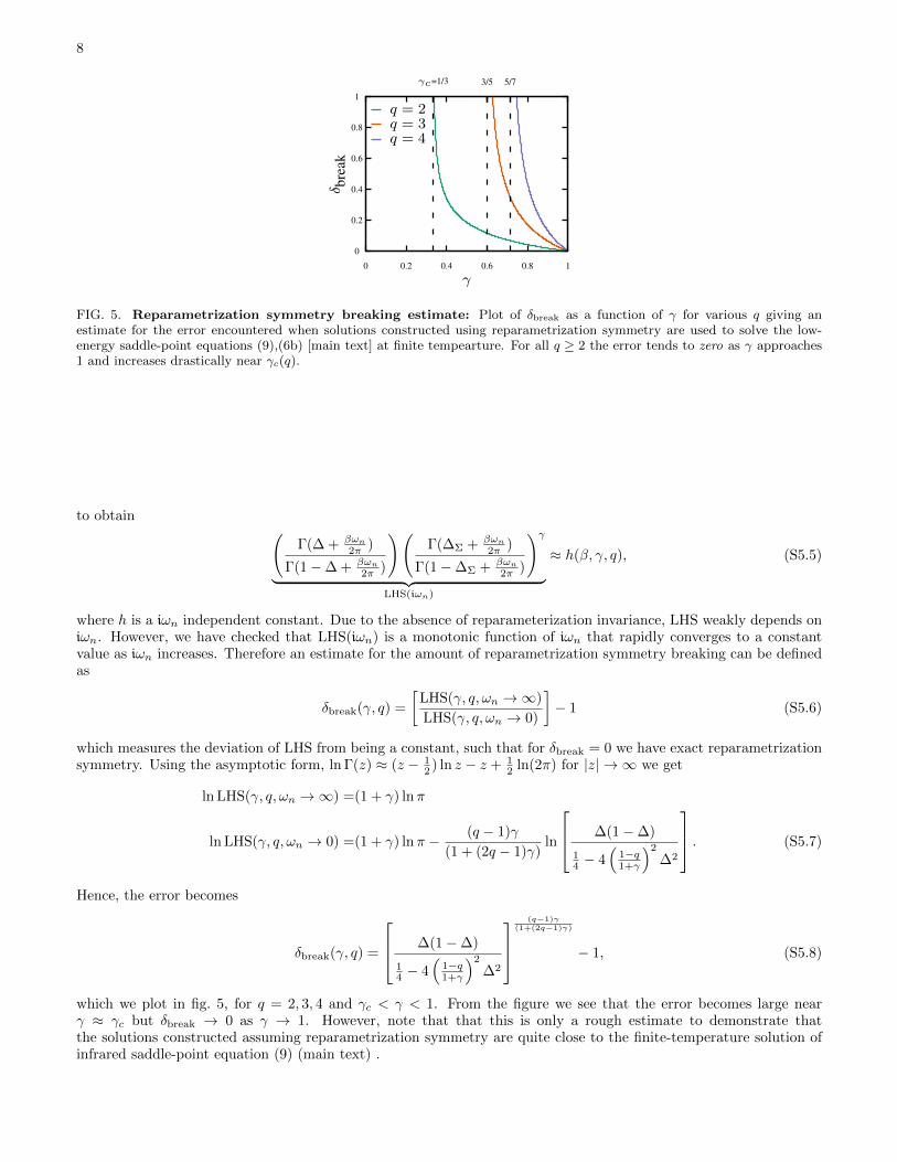
FIG. 5. Reparametrization symmetry breaking estimate: Plot of δbreak as a function of γ for various q giving anestimate for the error encountered when solutions constructed using reparametrization symmetry are used to solve the low-energy saddle-point equations (9),(6b) [main text] at finite tempearture. For all q ≥ 2 the error tends to zero as γ approaches1 and increases drastically near γc(q).

to obtain (Γ(∆ + βωn

2π )

Γ(1−∆ + βωn2π )

)(Γ(∆Σ + βωn

2π )

Γ(1−∆Σ + βωn2π )

)γ︸ ︷︷ ︸

LHS(iωn)

≈ h(β, γ, q), (S5.5)

where h is a iωn independent constant. Due to the absence of reparameterization invariance, LHS weakly depends oniωn. However, we have checked that LHS(iωn) is a monotonic function of iωn that rapidly converges to a constantvalue as iωn increases. Therefore an estimate for the amount of reparametrization symmetry breaking can be definedas

δbreak(γ, q) =

[LHS(γ, q, ωn →∞)

LHS(γ, q, ωn → 0)

]− 1 (S5.6)

which measures the deviation of LHS from being a constant, such that for δbreak = 0 we have exact reparametrizationsymmetry. Using the asymptotic form, ln Γ(z) ≈ (z − 1

2 ) ln z − z + 12 ln(2π) for |z| → ∞ we get

ln LHS(γ, q, ωn →∞) =(1 + γ) lnπ

ln LHS(γ, q, ωn → 0) =(1 + γ) lnπ − (q − 1)γ

(1 + (2q − 1)γ)ln

∆(1−∆)

14 − 4

(1−q1+γ

)2

∆2

. (S5.7)

Hence, the error becomes

δbreak(γ, q) =

∆(1−∆)

14 − 4

(1−q1+γ

)2

∆2

(q−1)γ

(1+(2q−1)γ)

− 1, (S5.8)

which we plot in fig. 5, for q = 2, 3, 4 and γc < γ < 1. From the figure we see that the error becomes large nearγ ≈ γc but δbreak → 0 as γ → 1. However, note that that this is only a rough estimate to demonstrate thatthe solutions constructed assuming reparametrization symmetry are quite close to the finite-temperature solution ofinfrared saddle-point equation (9) (main text) .

9

S6: Thermodynamics

The free-energy density for the system can be obtained by evaluating the action [eqn. (5), main text] using thesaddle point solutions, i.e.,

F =− T∑iωn

∫dεg(ε) ln [−iωn + ε+ Σ(iωn)]− J2

2q

∫ β

0

dτGq(β − τ)Gq(τ)− T∑iωn

Σ(iωn)G(iωn), (S6.1)

The entropy S is evaluated via S = −∂F/∂T .

a. Case – Non-Fermi liquid limit: We first derive an expression for entropy for the non-Fermi liquid case whenγ > γc(q) using the scaling solutions eqn. (S5.2). From eqn. (6b) in eqn. (S6.1) we get

F =−(

2q − 1

2q

)T∑n

Σ(iωn)G(iωn)︸ ︷︷ ︸F1

−T∑iωn

∫dεg(ε) ln [−iωn + ε+ Σ(iωn)]︸ ︷︷ ︸

F2

, (S6.2)

We consider the terms F1 and F2 separately below and obtain their leading low-temperature behaviors.

It can be shown that

∑iωn

Σ(iωn)G(iωn) =∑iωn

Σ(iωn)

1

NL

∑b,k

Gb(iωn,k)

=1

NL

∑b,k

∫dω

(ω − εb,k)ρb(ω,k)

1 + eβω,

where ρb(ω,k) = −(1/π)ImGb(iωn,k). Using the above we get

F1(T ) =1

NL

∑k,b

∫ ∞−∞

dω(ω − εb,k)ρb(ω,k)

1 + eβω=

∫ ∞−∞

dωωρ(ω)

1 + eβω︸ ︷︷ ︸F1a

−∫ ∞−∞

dω

∫ Λ

−Λ

dε εg(ε)ρ(ε, ω)

1 + eβω︸ ︷︷ ︸F1b

, (S6.3)

where ρ(ε, ω) = −(1/π)Im[(ω − ε− Σ(ω))−1] and ρ(ω) =∫ Λ

−Λdεg(ε)ρ(ε, ω). Due to particle-hole symmetry,

g(−ε) = g(ε), Σ′(−ω) = −Σ′(ω), Σ′′(−ω) = Σ′′(ω),

ρ(ε, ω) = ρ(−ε,−ω), ρ(ω) = ρ(−ω). (S6.4)

where Σ′ (Σ′′) are the real (imaginary) part of Σ(ω). Using these properties we obtain

F1a(T ) =2

∫ ∞0

dωωρ(ω)

1 + eβω−∫ ∞

0

dω ωρ(ω).

Since we are going to take a temperature derivative to obtain entropy, we subtract from above F1a(T = 0) =−∫∞

0dω ωρ(ω, T = 0). This takes care of the ultraviolet contribution that is not captured by the scaling solution of

eqn. (S5.2). Hence,

F1a(T )− F1a(T = 0) =−∫ ∞

0

dωω[ρ(ω)− ρ(ω, T = 0)] + 2

∫ ∞0

dωωρ(ω)

1 + eω/T.

Using the scaling form of eqn. (S5.2), we obtain for the two integrals above

2

∫ ∞0

dωωρ(ω)

1 + eω/T=2

A

J2∆T 2∆+1

∫ ∞0

duuϑ(u)

1 + eu∫ ∞0

dωω[ρ(ω)− ρ(ω, T = 0)] =A

J2∆T 2∆+1

∫ ∞0

duu[ϑ(u)− c1u2∆−1

].

Evidently, the integral in the first line is convergent, so there is no need for an ultraviolet cutoff. To check whetherthe integral in the second line is convergent, we check how the integrand behaves as u → ∞. It can be shown thatϑ(u) = c1u

2∆−1 + c2u2∆−3 + . . . for u → ∞ (see [22]). This gives an integrand c2u

2∆−2. For γc ≤ γ ≤ 1 we have−2 + 1/q ≤ 2∆− 2 ≤ −2 + 2/(2q − 1). Hence for q ≥ 2, the above integral is always convergent. From the above we

10

then find F1a ∼ T 2∆+1 so the contribution to entropy goes as

S1a ∼T 2∆. (S6.5)

Now, for F1b in eqn. (S6.3), using particle-hole symmetry we get

F1b(T ) =

∫ ∞0

dω

∫ Λ

−Λ

dε εg(ε)ρ(ε, ω) = − 1

πIm

[∫ ∞0

dω

∫ Λ

−Λ

dε εg(ε)G(ε, ω)

], (S6.6)

where G(ε, ω) ≡ (ω − ε− Σ(ω))−1. We can perform the integral over ε, as in eqn. (S3.1), in terms of the incompletebeta function and expand around Λ→∞ for ω Σ(ω) to get∫ Λ

−Λ

dε εg(ε)G(ε, ω) =− g0

[πe−i(π/2)(γ+1)Σ(ω)1−γ sec(γπ/2) +

2

γΛ1−γ + . . .

].

As earlier, we subtract F1b(T = 0) from F1b(T ) to obtain

F1b(T )− F1b(T = 0) =1

πIm

[g0π

e−i(π/2)(γ+1)

cos(γπ/2)

∫ ∞0

dω(Σ(ω)1−γ − Σ(ω, T = 0)1−γ)]

Again substituting the scaling form for Σ(ω) from eqn. (S5.3),

F1b(T )− F1b(T = 0) =1

πIm

[g0π

e−i(π/2)(γ+1)

cos(γπ/2)

(AΣ

J2∆Σ

)1−γ

T (2∆Σ−1)(1−γ)+1

∫ ∞0

du(fΣ(u)1−γ − c1−γ1 u(2∆Σ−1)(1−γ)

)].

(S6.7)

Using the the series expansion fΣ(u) = c1u2∆Σ−1 + c2u

2∆Σ−3 + . . . for u→∞, we get

fΣ(u)1−γ − c1−γ1 u(2∆Σ−1)(1−γ) '(1− γ)c−γ1 c2u(2∆Σ−1)(1−γ)−2. (S6.8)

Since ∆Σ ≤ 1 for γc ≤ γ ≤ 1, the integrand in eqn. (S6.7) is convergent for u → ∞. Hence we find F1b ∼T (2∆Σ−1)(1−γ)+1 implying that its contribution to the low-temperature entropy goes as

S1b ∼T (2∆Σ−1)(1−γ). (S6.9)

Comparing this with S1a in eqn. (S6.5) we find that S1b dominates over S1a for γc ≤ γ ≤ 1 as T → 0. Also, it can beshown from eqn. (S6.7) that S1b → 0 in the limit γ → 1, i.e., approaching the 0-dimensional SYK limit.

We now evaluate the contribution to entropy from the F2 in eqn. (S6.2). Following Ref.22, it can be shown that

F2 =

∫dε g(ε)

∫ ∞−∞

dω

π

(arctan

(G′(ε, ω)

G′′(ε, ω)

)− π

2

)nF (ω) =

∫ ∞−∞

dω

πnF (ω)

∫dε g(ε)

[arctan

(ω − ε− Σ′

|Σ′′|

)− π

2

],

(S6.10)

where G = G′+ iG′′, in terms of real and imaginary parts, and nF (ω) = 1/(eβω+1) is the Fermi function. To evaluatethe above, we use the identity

arctan

(ω − ε− Σ′

|Σ′′|

)− π

2=Re

[|Σ′′|

∫ 1

∞

dx

x2

1

(ω − ε− Σ′)− iΣ′′/x

].

The integral over ε in eqn. (S6.10) can now be performed, as in eqn. (S3.2), giving us

F2 =Re

g0π csc(γπ)(1− eiγπ)

∫ ∞−∞

dω

πnF (ω)

|Σ′′(ω)|(ω − Σ′(ω))γ

∫ 1

∞

dx

x2−γ1(

x− i Σ′′

ω−Σ′′

)γ .

11

The integral over x can also be easily performed to obtain

F2 =Re

[ig0π

1− γcsc(γπ)(1− eiγπ)

∫ ∞−∞

dω

πnF (ω)

((ω − Σ′(ω)− iΣ′′(ω))

1−γ − (ω − Σ′(ω))1−γ)].

Now we use the finite temperature scaling form of Σ(ω) from eqn. (S5.3) and neglect ω Σ(ω) in the above integral.In particular we have,

Σ′(ω) = AΣT2∆Σ−1 cot(π∆Σ)σ′

(ωT

)Σ′′(ω) = −AΣT

2∆Σ−1σ′′(ωT

)σ′(x) = sinh

(x2

)B(∆Σ + i x2π ,∆Σ − i x2π

)σ′′(x) = cosh

(x2

)B(∆Σ + i x2π ,∆Σ − i x2π

)where B(x, y) = Γ(x)Γ(y)/Γ(x + y) is the complete beta function, AΣ = AΣ/πJ

2∆Σ with AΣ is given in eqn. (S5.1)and 1− 1/2q ≤ ∆Σ ≤ 1. This results in

F2 =A1−γΣ T (2∆Σ−1)(1−γ)+1Re

[i(−1)1−γ g0π

1− γcsc(γπ)(1− eiγπ)

×∫ ∞−∞

du

π

1

eu + 1σ′′(u)1−γ

((cot(π∆Σ) tanh(u/2)− i)

1−γ − (cot(π∆Σ) tanh(u/2))1−γ)]. (S6.11)

The integral over u is convergent since B(x+ iy, x− iy) = |Γ(x+ iy)|2/Γ(2x) and |Γ(x+ iy)| y→∞=√

2πe−|y|/2|y|x−1/2

implying σ′′(u) → e−|u|/2 as |u| → ∞. Hence we find F2 ∼ T (2∆Σ−1)(1−γ)+1 with the corresponding contribution toentropy being

S2 ∼T (2∆Σ−1)(1−γ). (S6.12)

S2 has the same temperature dependence as S1b (see eqn. (S6.9)) and S1b+S2 dominates the low-temperature entropyfor γc ≤ γ ≤ 1, so that the total entropy

S ∼T (2∆Σ−1)(1−γ).

The above implies that the entropy increases rapidly, much faster than T , with increasing temperature as γ approaches1.

The residual entropy of the 0-dimensional SYK model can be recovered by carefully taking the limit γ → 1 ineqn. (S6.11). In this limit, g0/ csc(γπ)→ 1/2π. Using the identity, lnx = limx→0(xn − 1)/n

S(T = 0) =−∫ ∞−∞

du

π

1

eu + 1

(arctan(cot(π∆Σ) tanh(u/2))− π

2

).

For γ = 1 we have ∆ = 1/2q, ∆Σ = 1− 1/2q and cot(π∆Σ) = − cot(π∆). Hence,

S(γ → 1, T = 0) =

∫ ∞−∞

du

π

1

eu + 1

(arctan(cot(π∆) tanh(u/2)) +

π

2

)(S6.13)

which is exactly the expression for zero-temperature entropy for the 0-dimensional SYK model.

b. Case – Fermi liquid limit: The free-energy in the LFL regime can be obtained by neglecting the self-energycontributions in eqn. (S6.2) giving us

F =− T∑iωn

∫dεg(ε) ln [−iωn + ε] . (S6.14)

The sum over the Matsubara frequencies can be easily evaluated to get

F = −T∫

dεg(ε) ln [1 + exp(ε/T )] =− g0

∫ Λ

0

dε ε1−γ − 2g0T

∫ Λ

0

dε ε−γ ln [1 + exp(−ε/T )] . (S6.15)

12

=

=

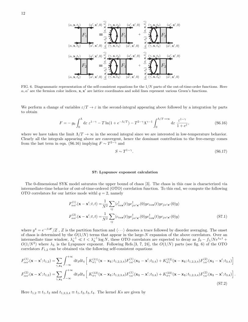
FIG. 6. Diagrammatic representation of the self-consistent equations for the 1/N parts of the out-of-time-order functions. Hereα, α′ are the fermion color indices, x,x′ are lattice coordinates and solid lines represent various Green’s functions.

We perform a change of variables ε/T → ε in the second-integral appearing above followed by a integration by partsto obtain

F =− g0

∫ Λ

0

dε ε1−γ − T ln(1 + e−Λ/T )− T 2−γΛγ−1

∫ Λ/T→∞

0

dεε1−γ

1 + eε, (S6.16)

where we have taken the limit Λ/T →∞ in the second integral since we are interested in low-temperature behavior.Clearly all the integrals appearing above are convergent, hence the dominant contribution to the free-energy comesfrom the last term in eqn. (S6.16) implying F ∼ T 2−γ and

S ∼ T 1−γ . (S6.17)

S7: Lyapunov exponent calculation

The 0-dimensional SYK model saturates the upper bound of chaos [3]. The chaos in this case is characterized viaintermediate-time behavior of out-of-time-ordered (OTO) correlation function. To this end, we compute the followingOTO correlators for our lattice mode withl q = 2, namely

F(1)αα′(x− x′; t, t) =

1

N2

∑ij

〈c†iαx(t)yc†jα′x′(0)yciαx(t)ycjα′x′(0)y〉

F(2)αα′(x− x′; t, t) =

1

N2

∑ij

〈ciαx(t)yc†jα′x′(0)yc†iαx(t)ycjα′x′(0)y〉 (S7.1)

where y4 = e−βH /Z , Z is the partition function and 〈· · · 〉 denotes a trace followed by disorder averaging. The onsetof chaos is determined by the O(1/N) terms that appear in the large-N expansion of the above correlators. Over anintermediate time window, λ−1

L t < λ−1L logN , these OTO correlators are expected to decay as f0 − f1/Ne

λLt +O(1/N2) where λL is the Lyapunov exponent. Following Refs.[3, 7, 24], the O(1/N) parts (see fig. 6) of the OTOcorrelators F1,2 can be obtained via the following self-consistent equations

F(1)αα′(x− x′; t1,2) =

∑γ,x1

∫ +∞

−∞dt3dt4

[K(11)αγ (x− x1; t1,2,3,4)F

(1)γα′(x1 − x′; t3,4) +K(12)

αγ (x− x1; t1,2,3,4)F(2)γα′(x1 − x′; t3,4)

]F

(2)αα′(x− x′; t1,2) =

∑γ,x1

∫ +∞

−∞dt3dt4

[K(12)αγ (x− x1; t1,2,3,4)F

(1)γα′(x1 − x′; t3,4) +K(22)

αγ (x− x1; t1,2,3,4)F(2)γα′(x1 − x′; t3,4)

].

(S7.2)

Here t1,2 ≡ t1, t2 and t1,2,3,4 ≡ t1, t2, t3, t4. The kernel Ks are given by

13

K(11)αγ (x− x1; t1,2,3,4) = 2J2GAγα(x1 − x; t31)GRαγ(x− x1; t24)G+

lr(t43)G−lr(t34)

K(12)αγ (x− x1; t1,2,3,4) =− J2GAγα(x1 − x; t31)GRαγ(x− x1; t24)G+

lr(t43)G+lr(t43)

K(21)αγ (x− x1; t1,2,3,4) =− J2GAγα(x1 − x; t42)GRαγ(x− x1; t13)G−lr(t34)G−lr(t34)

K(22)αγ (x− x1; t1,2,3,4) = 2J2GAγα(x1 − x; t42)GRαγ(x− x1; t13)G+

lr(t43)G−lr(t34) (S7.3)

where tij = ti − tj , GA(GR) is the advanced(retarded) Green’s functions and G±lr = G(it ± β/2) are Wightmanncorrelators obtained by contracting fermions with two different Keldysh indices (see [7, 24] for details). The convolutionover x1 in eqn. (S7.2) can be made into a product by moving to momentum representation, resulting in

F(1)αα′(q; t1,2) =

∑γ

∫ +∞

−∞dt3dt4

[K(11)αγ (q; t1,2,3,4)F

(1)γα′(q; t3,4) +K(12)

αγ (q; t1,2,3,4)F(2)γα′(q; t3,4)

]F

(2)αα′(q; t1,2) =

∑γ

∫ +∞

−∞dt3dt4

[K(12)αγ (q; t1,2,3,4)F

(1)γα′(q; t3,4) +K(22)

αγ (q; t1,2,3,4)F(2)γα′(q; t3,4)

], (S7.4)

where K(q) =∑xK(x)e−iq·x and F (q) =

∑xF (x)e−iq·x, respectively. To evaluate the Lyapunov exponent λL we use

the following chaos ansatz [3, 7]

F(i)αα′(q, t1,2) = eλL(q)(t1+t2)/2f

(i)αα′(q, t12) i = 1, 2. (S7.5)

Following Ref. 24, the time integrals in eqn. (S7.4) can be performed and the final result can be written as aneigenvalue equation in the real-frequency domain

|f(q, ω)〉 =

∫ +∞

−∞dω′

1

2π

2J2g1(ω − ω′)

[KRR KRB

KBR KBB

](q,−ω,λL)

−J2g2(ω′ − ω)

[KRR KRB

KBR KBB

](q,−ω,λL)

−J2g2(ω − ω′)[KRR KRB

KBR KBB

](q,ω,λL)

2J2g1(ω − ω′)[KRR KRB

KBR KBB

](q,ω,λL)

|f(q, ω′)〉,

(S7.6)where

|f(q, ω)〉 ≡

f

(1)RR(q, ω)

f(1)BR(q, ω)

f(2)RR(q, ω)

f(2)BR(q, ω)

(S7.7)

and

Kαα′(q, ω, λL) =1

Nk

∑k

GRαα′(q + k, ω + iλL/2)GAα′α(k, ω − iλL/2). (S7.8)

We now briefly discuss about the various Green’s functions that appear in eqn. (S7.6) and eqn. (S7.8). The functionsg1 and g2 are related to the Wightmann correlators in eqn. (S7.3) as

g1(ω) =

∫dt G+

lr(−t)G−lr(t)e

iωt

g2(ω) =

∫dt G+

lr(t)2eiωt =

∫dt G−lr(t)

2eiωt. (S7.9)

The Wightmann corellators G±lr(t) can be found by analytically continuing G(τ) as shown below

G+lr(t) =iG((τ > 0)→ it+

β

2)

G−lr(t) =iG((τ < 0)→ it− β

2), (S7.10)

14

which can also be written in the real frequency domain by using the spectral representation for G(τ) as

G±lr(ω) = ∓i πρ(ω)

cosh(ωβ/2), (S7.11)

where ρ(ω) = (−1/π)Im[G(ω+)]. The advanced and retarded Green’s functions can be obtained by analyticallycontinuing the following momentum-dependent Green’s function

Gαα′(k, iωn) =∑x

∫ β

0

dτ Gαα′(x, τ)eiωnτe−ik·x, (S7.12)

where Gαα′(x−x′, τ) = −〈cαx(τ)cα′x′(0)〉. Gαα′(k, iωn) can be written in terms of the Bloch fermion Green’s functionsG±(k, iωn), e.g., for a dispersion with even p in eqn. (S1.1) we get

GRR(k, iωn) = GBB(k, iωn) =1

2(G−(k, iωn) +G+(k, iωn))

GRB(k, iωn) = GBR(k, iωn) =1

2(G−(k, iωn)−G+(k, iωn)) , (S7.13)

where G±(k, iωn) = (iωn − ε±(k) − Σ(iωn))−1 [eqn. (7), main text]. At this point we set the dimension d to be oneand since we are interested in the low-energy physics we use

ε±(k) = ±Λ

∣∣∣∣kπ∣∣∣∣p , (S7.14)

instead of the high energy form in eqn. (S1.5) with Λ playing the role of the single-particle bandwidth. We mention herethat such a choice of parameters is used only to make the subsequent calculations easier and does not affect the finalresults for our system. Using eqn. (S7.13) and the symmetries available in our system, the various Ks in eqn. (S7.6)get related to each other. For example, because of color interchange symmetry, i.e. GRR(k, iωn) = GBB(k, iωn) andGRB(k, iωn) = GBR(k, iωn), we get

KRR(q, ω, λL) =KBB(q, ω, λL) ≡ K1(q, ω, λL)

KRB(q, ω, λL) =KBR(q, ω, λL) ≡ K2(q, ω, λL). (S7.15)

Also due to band inversion symmetry, i.e. ε±(k) = ε±(−k) and the relation GA−(+)(k, ω − iλ) =[GR−(+)(k, ω + iλ)

]∗we have

K1(2)(q, ω, λL) = K1(2)(−q, ω, λL) = K1(2)(q, ω, λL)∗. (S7.16)

Finally, due to the particle-hole symmetry

K1(2)(q, ω, λL) =K1(2)(q,−ω, λL)

g2(ω) =g2(−ω). (S7.17)

With the aid of the above relations, the eigenvalue eqn. (S7.6) attains the following nice structure

|f(q, ω)〉 =

∫ +∞

−∞dω′

1

2π

2J2g1(ω − ω′)

[K1 K2

K2 K1

](q,−ω,λL)

−J2g2(ω − ω′)[K1 K2

K2 K1

](q,−ω,λL)

−J2g2(ω − ω′)[K1 K2

K2 K1

](q,ω,λL)

2J2g1(ω − ω′)[K1 K2

K2 K1

](q,ω,λL)

|f(q, ω′)〉,

(S7.18)

15

which can be simplified by transforming f → h given byh

(1)q (ω)

h(2)q (ω)

h(3)q (ω)

h(4)q (ω)

=

f

(1)RR(q, ω) + f

(1)BR(q, ω)

f(1)RR(q, ω)− f (1)

BR(q, ω)

f(2)RR(q, ω) + f

(2)BR(q, ω)

f(2)RR(q, ω)− f (2)

BR(q, ω)

, (S7.19)

resulting in the following two decoupled eigenvalue equations[h

(1)q (ω)

h(3)q (ω)

]=

∫dω′

J2

2πKintra(q, ω, λL)

[2g1(ω − ω′) −g2(ω − ω′)−g2(ω − ω′) 2g1(ω − ω′)

][h

(1)q (ω′)

h(3)q (ω′)

](S7.20)[

h(2)q (ω)

h(4)q (ω)

]=

∫dω′

J2

2πKinter(q, ω, λL)

[2g1(ω − ω′) −g2(ω − ω′)−g2(ω − ω′) 2g1(ω − ω′)

][h

(2)q (ω′)

h(4)q (ω′)

]. (S7.21)

The new Kernels Kintra, Kinter are related to the old ones by

Kintra(q, ω, λL) =K1(q, ω, λL) + K2(q, ω, λL)

Kinter(q, ω, λL) =K1(q, ω, λL)− K2(q, ω, λL). (S7.22)

The meaning of the subscripts intra/inter in the Kernels becomes evident when we write them explicitly in terms ofthe Bloch fermion Green’s functions, i.e.,

Kintra(q, ω, λL) =1

Nk

∑k

1

2

(GR+(q + k, ω + iλL/2)GA+(k, ω − iλL/2) +GR−(q + k, ω + iλL/2)GA−(k, ω − iλL/2)

)Kinter(q, ω, λL) =

1

Nk

∑k

1

2

(GR+(q + k, ω + iλL/2)GA−(k, ω − iλL/2) +GR−(q + k, ω + iλL/2)GA+(k, ω − iλL/2)

),

(S7.23)

which shows that the intraband mode involves the sum of terms that operate within a band whereas the interbandmode involves terms that operate across bands. Henceforth we focus on the q = 0 mode of the above equations,which can then be explicitly written as

K(q=0)intra (ω) =

∫ Λ

−Λ

dεg(ε)

(ω − iλL/2− ε− Σ(ω − iλL/2))(ω + iλL/2− ε− Σ(ω + iλL/2))

K(q=0)inter (ω) =

∫ Λ

−Λ

dεg(ε)

(ω − iλL/2− ε− Σ(ω − iλL/2))(ω + iλL/2 + ε− Σ(ω + iλL/2)), (S7.24)

where we have substituted the expression for GA(R)± (k, ω± iλL/2) by analytically continuing eqn. (7) (main text). The

self-energy Σ(ω ± iλL/2) can be obtained from the spectral function ρΣ(ω) = (−1/π)Im[Σ(ω+)] by using the integralrepresentation

Σ(z = ω ± iλL/2) =

∫ +∞

−∞dω

ρΣ(ω)

z − ω. (S7.25)

The above equations for K(q=0)intra and K

(q=0)intra also tells us that the information from the lattice, like dimension etc.,

enters implicitly through the density of states g(ε), hence the obtained expressions are general and should be validfor arbitrary dimensions d ≥ 1 as well.

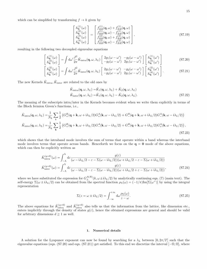
1. Numerical details

A solution for the Lyapunov exponent can now be found by searching for a λL between [0, 2π/T ] such that theeigenvalue equations (eqn. (S7.20) and eqn. (S7.21)) get satisfied. To this end we discretize the interval [−Ω,Ω], where

16

0

0.2

0.4

0.6

0.8

1

0 0.1 0.2 0.3 0.4 0.5 0.6 0.7 0.8 0.9 1

λ(q

=0

)

L(i

nter

)/2πT

T

γ = 0.45γ = 0.5γ = 0.6γ = 0.7γ = 0.8γ = 0.9γ = 0.95SYK

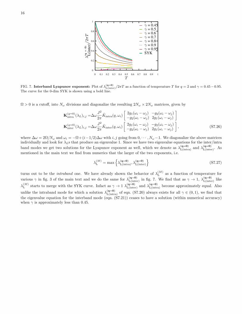
FIG. 7. Interband Lyapunov exponent: Plot of λ(q=0)L(inter)/2πT as a function of temperature T for q = 2 and γ = 0.45−0.95.

The curve for the 0-dim SYK is shown using a bold line.

Ω > 0 is a cutoff, into Nω divisions and diagonalize the resulting 2Nω × 2Nω matrices, given by

K(q=0)intra (λL)i,j =∆ω

J2

2πKintra(q, ωi)

[2g1(ωi − ωj) −g2(ωi − ωj)−g2(ωi − ωj) 2g1(ωi − ωj)

]K

(q=0)inter (λL)i,j =∆ω

J2

2πKinter(q, ωi)

[2g1(ωi − ωj) −g2(ωi − ωj)−g2(ωi − ωj) 2g1(ωi − ωj)

], (S7.26)

where ∆ω = 2Ω/Nω and ωi = −Ω+(i−1/2)∆ω with i, j going from 0, · · · , Nω−1. We diagonalize the above matricesindividually and look for λLs that produce an eigenvalue 1. Since we have two eigenvalue equations for the inter/intra

band modes we get two solutions for the Lyapunov exponent as well, which we denote as λ(q=0)L(intra) and λ

(q=0)L(inter). As

mentioned in the main text we find from numerics that the larger of the two exponents, i.e.

λ(M)L = max

λ

(q=0)L(intra), λ

(q=0)L(inter)

(S7.27)

turns out to be the intraband one. We have already shown the behavior of λ(M)L as a function of temperature for

various γ in fig. 3 of the main text and we do the same for λ(q=0)L(inter) in fig. 7. We find that as γ → 1, λ

(q=0)L(inter) like

λ(M)L starts to merge with the SYK curve. Infact as γ → 1 λ

(q=0)L(inter) and λ

(q=0)L(intra) become approximately equal. Also

unlike the intraband mode for which a solution λ(q=0)L(intra) of eqn. (S7.20) always exists for all γ ∈ (0, 1), we find that

the eigenvalue equation for the interband mode (eqn. (S7.21)) ceases to have a solution (within numerical accuracy)when γ is approximately less than 0.45.