HIGH-SPEED HIGH-RESOLUTION VECTOR FIELD …
154
HIGH-SPEED HIGH-RESOLUTION VECTOR FIELD MEASUREMENTS AND ANALYSIS OF BOUNDARY LAYER FLOWS IN AN INTERNAL COMBUSTION ENGINE by Ali Alharbi A dissertation submitted in partial fulfillment of the requirements for the degree of Doctor of Philosophy (Mechanical Engineering) in The University of Michigan 2010 Doctoral Committee: Professor Volker Sick, Chair Professor Steven L. Ceccio Associate Professor Luis P. Bernal Visiting Research Scientist David L. Reuss
Transcript of HIGH-SPEED HIGH-RESOLUTION VECTOR FIELD …
HIGH-SPEED HIGH-RESOLUTION VECTOR FIELD MEASUREMENTS AND
ANALYSIS OF BOUNDARY LAYER FLOWS IN AN INTERNAL COMBUSTION
ENGINE
by
Ali Alharbi
A dissertation submitted in partial fulfillment
of the requirements for the degree of
Doctor of Philosophy
(Mechanical Engineering)
in The University of Michigan
2010
Doctoral Committee:
Professor Volker Sick, Chair
Professor Steven L. Ceccio
Associate Professor Luis P. Bernal
Visiting Research Scientist David L. Reuss

ii
DEDICATION
To my lovely family
iii
ACKNOWLEDGEMENTS
This work would not have been possible without the help and support from a
number of people. First I would like to thank my advisor, Professor Volker Sick, for
introducing me to the fascinating world of experimental fluid mechanics. His guidance
and support throughout my work have been indefinite, and his knowledge has been a
great source of inspiration.
I would like to thank my committee members, Professor Steven Ceccio, Professor
Luis Bernal, and Dr. David Reuss for being part of this work. It is an honor having you in
my Doctoral committee. I would like to acknowledge Professor Matthias Ihme and
Professor David Dowling for their valuable discussions and recommendations which
added depth to my work and helped broaden my knowledge in turbulence.
I would like to thank my former and current colleagues from the quantitative laser
diagnostics lab for their help with experiments and for being such a wonderful friends,
Dr. James Smith, Western Michigan University Assistant Professor Claudia Fajardo, Dr.
Rui Zhang, Brian Peterson, Mike Cundy, Kevin Peterson, Mike Mosburger, Preeti
Abraham, Louise Lu, Omar Almagri, Hao Chen, Mike Litsey, Jessamyn Margoni, Mike
Chin, Daniel Rimmelspacher, Patrick Nohe, and Jason Moscetti.

iv
I would like to thank my mother and father for their unconditional love and
support throughout the years, my two lovely sisters and my brothers for being so kind. I
would like to thank my wife for her sacrifices. This is the second time you set your career
aside so we can be together. I know if you had to, you would do this million times again.
Last, I would like to thank the Public Authority for Applied Education and
Training (PAAET) for sponsoring me the past five years. And I would like to
acknowledge my PAAET advisor at Kuwait embassy, Ms. Shoghig Sahakyan, for her
support throughout my entire study period.

v
TABLE OF CONTENTS
DEDICATION .................................................................................................................... ii
ACKNOWLEDGEMENTS ............................................................................................... iii
LIST OF FIGURES ......................................................................................................... viii
LIST OF TABLES ............................................................................................................ xii
ABSTRACT ..................................................................................................................... xiii
CHAPTER 1 INTRODUCTION ....................................................................................... 1
CHAPTER 2 INTERNAL COMBUSTION ENGINE HEAT TRANSFER ..................... 5
2.1 Importance and Uniqueness of IC Engine Heat Transfer ....................................... 6
2.2 Combustion Chamber Heat Transfer: Cycle Description ....................................... 7
2.3 Heat Transfer Mechanisms ..................................................................................... 9
2.3.1 Conduction in the Solid Parts ........................................................................ 9
2.3.2 Convection in the gas side ............................................................................. 9
2.3.3 Radiation Heat Transfer ............................................................................... 17
2.4 Literature Review on Gas Side Convective Heat Transfer ................................... 19
2.4.1 Global Models .............................................................................................. 20
2.4.1.1 Time-Averaged Heat Flux Correlations.............................................. 20
2.4.1.2 Instantaneous Spatial Average Correlations ....................................... 21
2.4.1.3 Instantaneous Local Correlations ........................................................ 25
2.4.2 Zonal Models ............................................................................................... 31
2.4.3 One Dimensional and Three Dimensional CFD Models ............................. 32
CHAPTER 3 FLOW IN THE CYLINDER ..................................................................... 34

vi
3.1 Major Fluid Motions in the Cylinder .................................................................... 35
3.1.1 Tumble and Swirl Mean Flows .................................................................... 35
3.1.2 Squish ........................................................................................................... 37
3.2 Mean Velocity and Turbulence Characteristics .................................................... 37
3.3 Mean Flow Equations ........................................................................................... 40
3.3.1 Boundary Layer Equations for Plane Flows ................................................ 45
3.3.2 The Universal Law of the Wall .................................................................... 48
3.4 Analysis of Instantaneous Velocity Vector Fields ................................................ 52
3.4.1 Visualization of Vortices ............................................................................. 53
3.4.2 Vortex Identification .................................................................................... 55
3.5 Experimental Flow Diagnostic Techniques and Their Applications to IC
Engines ........................................................................................................................ 56
3.5.1 Laser Doppler Velocimetry .......................................................................... 56
3.5.2 Particle Image Velocimetry ......................................................................... 58
3.6 Literature Review on Near-Wall Velocity Measurements on IC Engines and
the Structures of Turbulent Boundary Layer .............................................................. 61
CHAPTER 4 PIV AND PTV PARAMETER OPTIMIZATIONS AND ERROR
ANALYSIS ....................................................................................................................... 75
4.1 PIV Parameters ..................................................................................................... 75
4.1.1 Imaging System ........................................................................................... 75
4.1.2 Particle Image Shift...................................................................................... 77
4.1.3 Seeding Tracking ......................................................................................... 78
4.1.4 Particle Image Density ................................................................................. 81
4.2 Error Analysis ....................................................................................................... 82
4.2.1 Systematic Error........................................................................................... 82
4.2.2 Random Errors ............................................................................................. 83

vii
4.2.2.1 Calibration (α) ..................................................................................... 83
4.2.2.2 Displacement of Particle Image (ΔX) ................................................. 86
4.2.2.3 Time Interval (Δt) ............................................................................... 88
4.2.2.4 Seeding Velocity Lag (δu) .................................................................. 88
CHAPTER 5 LOW AND HIGH RESOLUTION PIV EXPERIMENTS NEAR THE
CYLINDER HEAD .......................................................................................................... 90
5.1 Experiment ............................................................................................................ 91
5.1.1 Setup ............................................................................................................ 91
5.1.2 Data Acquisition .......................................................................................... 97
5.1.3 Data Processing ............................................................................................ 98
5.2 Measurement Uncertainty ................................................................................... 101
5.3 Results and Discussion ....................................................................................... 102
5.3.1 Mean Velocity and Fluctuation Intensity Profiles ..................................... 104
5.3.2 Vortex Visualization and Identification ..................................................... 109
5.3.3 Continuity Equation ................................................................................... 117
5.3.4 The Law of the Wall .................................................................................. 121
CHAPTER 6 CONCLUSIONS AND FUTURE WORK .............................................. 131
BIBLIOGRAPHY ........................................................................................................... 136

viii
LIST OF FIGURES
Figure 2-1: Thermal boundary layer ................................................................................. 11
Figure 2-2: Schematic of heat transfer flow from combustion chamber to the coolant
through cylinder wall .................................................................................. 19
Figure 2-3: Overall engine heat transfer coefficient. µg: gas viscosity, kg: gas thermal
conductivity, m: charge mass flow rate (6). ................................................ 21
Figure 2-4: Thermocouple locations on cylinder head and wall (14). .............................. 27
Figure 2-5: Instantaneous temperature distribution at different locations (14). ............... 27
Figure 2-6: Comparisons of predictions of previous correlations with experimental data
(14). ............................................................................................................. 28
Figure 2-7: locations of heat flux probes (15). ................................................................. 29
Figure 2-8: Instantaneous temperature distribution measured at various locations on the
piston top and cylinder head (15). ............................................................... 30
Figure 2-9: Instantaneous heat flux at different locations for a homogenous charge spark
ignition engine (left) and the HCCI engine (right) (15). ............................. 30
Figure 3-1: Schematic of tumble and swirl, Wilson et al. (20)......................................... 36
Figure 3-2: Schematic of how piston motion generates squish (2). .................................. 37
Figure 3-3: Velocity vector grid. ...................................................................................... 47
Figure 3-4: Radial distribution of mean tangential velocity at half of the clearance height
(33). ............................................................................................................. 58
Figure 3-5: LDV measurement locations in the center of the clearance height (42). ....... 61
Figure 3-6: (left) Ensemble averaged mean velocity profiles measured in non-firing
cycles, (right) Magnified view From Figure 3.5 (42). ................................ 62
Figure 3-7: (left) Ensemble averaged mean velocity profiles measured in firing cycles,
(right) Magnified view From Figure 3.6 (42). ............................................ 63

ix
Figure 3-8: Schematic of the engine combustion chamber (43). ...................................... 64
Figure 3-9: Boundary layer velocity profiles for the high swirl case (43)........................ 66
Figure 3-10: Boundary layer velocity profiles for the low swirl case (43). ...................... 67
Figure 3-11: Schematic of the bottom view of cylinder head (top) and clearance volume
(bottom) of the four stroke engine used for the LDV measurements in
experiment 1 and 2 (44). ............................................................................. 69
Figure 3-12: Velocity vectors for the 750 rpm high swirl case at 220 degrees (44). ........ 69
Figure 3-13: Porting geometry and field of view for experiment 3 (no boost port, M=0.83
and M=1.0), experiment 4 and 5 (with boost port, M=1) (44). ................... 70
Figure 3-14: Schematic of head detail of the combustion chamber for experiment 3 (left),
experiment 4 (left portion of the image on right), and experiment 5 (left
portion of the image on right) (44). ............................................................. 70
Figure 4-1: Geometric image construction. ...................................................................... 76
Figure 4-2: Calibration plate positioning in the laser sheet plane (image plane). ............ 84
Figure 5-1: Schematic of the optical SIDI engine. Field of view shown on the right image
is for the high resolution experiment. The low resolution measurements
cover the entire area between the spark plug and the fuel injector ............. 91
Figure 5-2: Light sheet position on the cylinder head between spark plug and injection,
viewed from bottom of the engine (57). Indicated field of view location is
for the low resolution experiment. The high resolution field of view is
within the range shown as in the right of Figure 5-1................................... 92
Figure 5-3: A) HR532 mirror, B) telescope lens, C) 45º mirror, D) long distance
microscope. ................................................................................................. 95
Figure 5-4: Initiation and progression of flow reversal during the expansion stroke. Spark
plug and fuel injector are located to the right and left of each image,
respectively. Measurements obtained from the low resolution experiment.
................................................................................................................... 103
Figure 5-5: Ensemble-averaged velocity vector fields for crank angle 180. The
highlighted area shows the region from where the horizontal (x-) velocity
component of seven adjacent vertical profiles are spatially averaged and
then are used for further analysis. Shown in the background is a raw image
of seeded flow. Note that for clarity in this image only every fourth vector
in each direction is displayed to allow visualization of the vector tip. ..... 104

x
Figure 5-6: Seven velocity profiles were used to determine a spatially averaged (over 315
μm) velocity profile to improve the statistical significance of the velocity
data closest to the surface. The example shown was taken at 180 CAD and
shows the low variation across the averaged region, justifying this
approach. ................................................................................................... 105
Figure 5-7: Ensemble-averaged velocity profile as a function of crank angle during the
compression stroke and most of the expansion stroke (180 to 490 CAD). 106
Figure 5-8: Ensemble-averaged velocity profiles at selected CAD during the end of the
compression stroke and most of the expansion stroke. ............................. 107
Figure 5-9: Fluctuation intensity profile as a function of crank angle (180 to 450 CAD).
................................................................................................................... 109
Figure 5-10: a) Low resolution instantaneous flow field decomposed using a number of
Galilean convection velocities: b) Uc = 0.7 the maximum velocity of the
ensemble averaged flow field (Umax,mean), c) Uc= 0.5 Umax,mean, d) Uc = 0.3
Umax.mean, e) Uc = instantaneous velocity field spatial average, f) Reynolds
decomposition, g) high pass LES, h) low pass LES. ................................. 113
Figure 5-11: Swirling strength map superimposed on the different decompositions of the
instantaneous flow field described in Figure 5-10. ................................. 114
Figure 5-12: High resolution instantaneous velocity vector field decomposed using high
pass LES filter applied over a 0.225 mm domain (5 grid spacing). .......... 115
Figure 5-13: High resolution instantaneous velocity vector field decomposed using high
pass LES filter applied over a 225 μm domain (5 grid spacing) (top image)
and a 90 μm domain (2 grid spacing) (bottom image). ............................. 116
Figure 5-14: Difference between Favre averages and ensemble averages. .................... 118
Figure 5-15: Divergence and temporal density gradient versus CAD. ........................... 119
Figure 5-16: Spark plug impact on enhancing the third velocity (z-) component. ......... 120
Figure 5-17: Divergence of the ensemble averaged velocity fields at selected CAD .... 121
Figure 5-18: Experimental results of velocity profiles compared to viscous sublayer and
log layer at selected CAD. ......................................................................... 123
Figure 5-19: Low and high resolution velocity profiles at 200 CAD. ............................ 125
Figure 5-20: Normalized Reynolds stresses at selected CAD. ....................................... 127
Figure 5-21: Production and dissipation of turbulent kinetic energy at selected CAD. . 128

xi
Figure 5-22: Turbulent kinetic energy production, Reynolds shear stress, and mean
velocity profile at 186 CAD. ..................................................................... 130
xii
LIST OF TABLES
Table 5.1: Optical SIDI engine specifications. Note: valves timings are with 0.1 mm lift.
..................................................................................................................... 92
Table 5.2: PIV parameters ................................................................................................ 95
Table 5.3: Particle time scale, flow time scales, and the corresponding Stokes number as
a function of CAD. ...................................................................................... 97
Table 5.4: Summary of uncertainty terms for the high resolution experiment ............... 101
Table 5.5: Combined velocity uncertainty ...................................................................... 102
Table 5.6: Standard deviation of seven adjacent horizontal velocity components as a
function of distance from the wall for selected CAD. ............................... 105
xiii
ABSTRACT
Heat transfer properties vary locally and temporally in internal combustion
engines due to variations in the boundary layer flow. In order to characterize the
dynamics in the boundary layer, crank-angle resolved high-speed Micro Particle Image
Velocimetry (μPIV) and Particle Tracking Velocimetry (PTV) have been used for near-
wall velocity measurements in a spark-ignition direct-injection single cylinder engine. A
527 nm dual cavity green Nd:YLF laser was used for velocity measurements near the
cylinder head wall between the intake and exhaust valves in the tumble mean flow plane
parallel to the cylinder axis. A long distance microscope was used to obtain a spatial
resolution of 45 µm. Flow fields were determined from 180 to 490 CAD in the
compression and expansion strokes. The accomplished experiment represents first-time
two-dimensional and a time history velocity measurements in a boundary layer flow in
internal combustion engine. The data shows significant variation in the flow during the
compression and expansion strokes and from cycle to cycle. Flow deceleration was
observed during the end of the compression which continued during the expansion stroke
until 400 CAD when the flow direction reverses. Submillimeter sized vortical structures
were observed within the boundary layer over extended periods of time. Inner length and
velocity scales were determined from the experimental results and were used to construct
the law of the wall velocity distribution in the viscous sublayer and in the log law region.
Experimental velocity profiles show agreement with the law of the wall in the viscous
xiv
sublayer but they exhibit an early departure in the log law region due to the unique nature
of the tumbling free stream flow in internal combustion engines. Reynolds stresses in the
plane flow along with turbulent kinetic energy production and dissipation were
determined.
1
CHAPTER 1
INTRODUCTION
In-cylinder convection heat transfer from the gas side to the walls of the
combustion chamber of an IC engine plays an important role on the performance and
design of engines. Since the 1920’s, many experiments have been conducted producing a
handful empirical correlations for the heat transfer coefficient. Many of these correlations
once were widely used and then became obsolete with the introduction of other
correlations that utilized a wider range of data and different approaches leading to more
universal formulas. Almost all of the proposed correlations for the past eighty years give
spatially averaged heat transfer coefficient; thus lack detailed description of local
convection heat transfer. Another issue with the spatially averaged correlations is that
they are experimentally determined based on heat flux and wall temperature
measurements in single point on the combustion chamber. As will be seen on the
literature review on the instantaneous local correlation section that wall temperature; and
therefore heat flux, varies spatially at any instant during the cycle. Energy balance
methods to determine the spatially averaged heat transfer coefficient should remedy this
issue; however, it still does not give detailed local description of heat transfer.

2
With the vast developments of computing capabilities, multidimensional
numerical simulations offer a great alternative that provides a comprehensive analysis of
fluid flow and heat transfer process. However; the flow being unsteady and turbulent,
modeling of the turbulent terms of the governing transport equations remains a
challenging task. Experimental work is needed to provide modelers with the data to
validate and improve current modeling methods. After detailed study of the status of heat
transfer in IC engines, Borman and Nishiwaki (1) concluded that the fundamental
problem in modeling is the lack of detailed data regarding the gas side velocity and
temperature distribution, and vital questions concerning the turbulent boundary layer
model need to be explored experimentally. They recommend that a fundamental work on
convective heat transfer is needed applying modern optical methods to determine
velocity, temperature, and turbulence profiles. Even though their study was carried out
twenty three years ago, not much has been done to fulfill the recommended experimental
work leaving the fundamental problem of convective heat transfer problem in internal
combustion engines unaddressed and requiring more attention.
A number of in cylinder flow measurements have been conducted using methods
like hot wire anemometry, laser Doppler velocimetry (LDV), and particle image
velocimetry (PIV) studying instantaneous and bulk velocities, turbulence intensities,
vorticity and strain rates, cycle-to-cycle variability, and mean flows, i.e. swirl and tumble.
However, only few attempts have been made to measure near-wall velocity distribution.
LDV was the only tool applied to those studies giving high temporal resolutions at one
point in the flow. These experiments often used special designs for the cylinder head in

3
order to get closer to the wall. When a more realistic simple flat head was under study,
the closest distance to the engine head was approximately four times the one for the
specially designed cylinder head.
The purpose of the current research is to apply a more versatile method to resolve
near-wall velocities in actual production engine design. PIV was applied to measure near-
wall velocities at the cylinder head. Based on preliminary experiments, higher
magnifications were required to zoom in the boundary layer region. A long distance
microscope was used to resolve the hydrodynamic boundary layer near the cylinder head
wall. Prior to that high resolution PIV experiment, a low resolution PIV experiment was
conducted to obtain an overview of the flow behavior near the cylinder head wall in the
region between the spark plug and the fuel injector of the optical spark ignited direct
injection engine. Low seeding count in the high resolution μPIV experiment was rectified
by applying a hybrid algorithm combining PIV as a “predictor” of the flow field and
particle tracking velocimetry (PTV) as a “corrector” of the flow field by tracking
individual particles. The PTV algorithm also helped increase the resolution of the
measurement and reduce near wall bias. Another challenge was the drawback of
conducting a PIV experiment near a wall, which is glare caused by laser reflection off the
wall surface that may exceed the Mie scattering signal of the seeding particles. A flat
black paint was used on the surface of interest, which helped reducing the intensity of the
reflection drastically.
4
In this document, heat transfer in IC engines is discussed in Chapter two. It covers
the importance and uniqueness of in cylinder heat transfer, cycle description of heat
transfer, heat transfer mechanisms with an emphasis on convection heat transfer. It ends
with a literature review on global and zonal heat transfer coefficient correlations, and one
dimensional and three dimensional models. Chapter three goes over the major mean flow
induced motions, i.e. swirl and tumble, mean velocity and turbulence characteristics,
mean flow equations including boundary layer approximations and the universal law of
the wall, experimental flow diagnostic techniques and their applications to IC engines,
and a literature review on near-wall velocity measurements in IC engines. In chapter four,
PIV parameters optimization and error analysis are discussed. In chapter five,
experimental setup for both the low resolution and high resolution experiments is
described, followed by data processing method applied to each experiment, and ending
with results and discussion. Results and issues arose during both experiments are
concluded in chapter 6 along with a discussion on suggested modifications to minimize
those issues. At the end of chapter 6, a discussion of future work is presented and
recommendations are suggested.
5
CHAPTER 2
INTERNAL COMBUSTION ENGINE HEAT TRANSFER
One of the main reasons this research is carried out is to help provide the means to
understand and develop modeling heat transfer analysis in internal combustion engines.
Internal combustion engines heat transfer is considered one of the most difficult, if not
the most difficult, heat transfer problems. Due to its extreme importance on engines
design and performance, researchers utilized different approaches for the past eighty
years trying to come up with the ultimate solution for the combustion chamber heat
transfer process. However, because of its complexity, no detailed solution (i.e., local and
instantaneous) have been verified.
This chapter on IC engines heat transfer is intended to show during its course the
importance of a major heat transfer mechanism in IC engines which is convective heat
transfer. As will be seen in the literature review, different models have been proposed
during the last eighty years; however, no experimental work has been done for the gas
side convective heat transfer to predict the local and instantaneous heat transfer
coefficient. With the advances of optical engines diagnostics, engine researches are one
step closer to resolve hydrodynamic boundary layer on cylinder head and walls, which
should give modelers a more accurate velocity profile to implement on their codes rather
than the turbulent “law of the wall” which is often used in most models.

6
It is a common practice when studying the IC engine heat transfer to divide the
engine into subsystems (1) and (2). Intake and exhaust are considered two subsystems.
Coolant is the third subsystem and lubricating oil is the fourth subsystem. The fifth
subsystem is the combustion chamber which is the most important part of the engine and
the source of all difficulties. The sixth subsystem is the solid parts that the previous
subsystems are made of. In this current research, only the combustion chamber subsystem
is considered for boundary layer investigation. Other subsystems, even though they have
significant impact on the engine heat transfer problem, are not considered here.
In this chapter, the importance of studying IC engines heat transfer is emphasized
by first showing a brief description of its uniqueness and sources of difficultly followed
by a step by step analysis of the heat transfer process during the IC engine cycle. Heat
transfer mechanisms are then reviewed and then followed by background literature on the
combustion chamber heat transfer.
2.1 Importance and Uniqueness of IC Engine Heat Transfer
During the combustion process in IC engines, burned gas temperature reach
values in the neighborhood of 2500 K. Exhaust gas temperature is of order 1300 K.
Knowing that Aluminum melting point is about 933 K and iron melting point is 1808 K,
coolant system must be provided to ensure that piston, cylinder, and valves temperatures
are kept below those critical temperatures. In fact, metal temperature must even stay
much lower than those temperatures to insure that its strength does not degrade. Heat flux
during combustion reaches a maximum of about 10 MW/m2 in some parts of the engine
and then drops to zero during another cycle stage. This heat flux fluctuation happens in a

7
matter of milliseconds causing a lot of thermal stresses on engine regions affected by
such fluctuations; therefore, these regions must be thermally controlled by means of
cooling systems to keep them at or below 673 K for iron and 573 K for aluminum alloys.
In addition to temporal heat flux fluctuations during one cycle, spatial variation is another
source of engine heat transfer difficulty, heat flux vary by as much as 5 MW/m2 between
two spots 1 cm apart. What makes heat flux issue even more complex is that this
temporal and spatial pattern varies from cycle to cycle. To avoid lubricating oil
deterioration, gas side wall temperatures must be kept below 450 K. Spark plug and
exhaust valves, which are usually the hottest parts of the combustion chamber, must be
kept cool to avoid pre-ignition problems. Cooling process must be optimized in a way to
control the amount of heat transferred to the walls since higher heat transfer to the wall
will lower the charge temperature and gas pressure, and therefore reduce the work output.
So heat transfer also affects engine performance and efficiency. Another major effect of
engine heat transfer is emissions where analysis of such problem must include, in
addition to the combustion chamber, the exhaust system which is not the focus of the
current research. (2) and (3).
2.2 Combustion Chamber Heat Transfer: Cycle Description
Whether the heat is transferred to or from the walls depends on the operating
condition. In general, during the intake stroke, as charge enters the intake port, heat is
transferred from the port walls and intake valves to the gas. More heat is transferred to
the gas as the charge enters the cylinder drawing more energy from the combustion
chamber walls. Even though this process helps vaporizing the fuel and also brings the
energy back to the combustion chamber via the intake charge, it reduces the volumetric

8
efficiency of the engine. During compression, the charge temperature increases to
temperatures higher than the combustion chamber walls. Heat is transferred from the gas
side to cylinder walls. The importance of heat transfer during the compression stroke is in
its effect on knock on SI engines and on ignition timing on CI engines. One-zone models,
which will be discussed later, do not determine bulk gas temperature differences within
the combustion chamber. The major drawback of one-zone models is that they do not
take into account the boundary layer gas which contains a considerable amount of the
cylinder mass approximated by 10-20 %. Two-zone model having the core gas as one
zone and boundary layer gas as the other zone gives a gas core temperature that is 100-
200ºC higher than the mass averaged one zone models (4). This huge discrepancy
between the one-zone models and the two-zone models show that there is a need for
accurate temperature distribution within the combustion chamber. Heat transfer rates to
the walls are the highest during the combustion stage. Gas temperatures increase
substantially and fluid motion also increases and continues to do so during the expansion
stroke which results in an enhanced forced convection heat transfer to the walls. Higher
pressures during combustion force the cylinder gas into crevices which also adds to the
heat transfer to the combustion chamber walls. During the expansion stroke, heat transfer
rates decrease due to drop in gas temperature and convection heat transfer coefficients
which are reduced because of the decrease in gas density during expansion. During
blowdown and exhaust, high velocities are generated causing an increase of heat transfer
to the exhaust valves and exhaust port walls (1).

9
2.3 Heat Transfer Mechanisms
The three mechanisms of heat transfer are present in IC engines. Conduction
through solids (the sixth subsystem), gas side convection, and radiation from combustion
gases to the walls. Conduction and radiation heat transfer are not the focus of the current
research; however, a brief description is given below for each of the three heat transfer
modes.
2.3.1 Conduction in the Solid Parts
Heat transfer in the solid parts, previously categorized as the sixth subsystem,
occurs by means conduction. Conduction heat transfer is described as heat transfer by
molecular motion in solids and fluids at rest due to temperature gradient. It is governed
by Fourier’s law as follows:
q k T (2.1)
where k is the thermal conductivity. For steady one-dimensional temperature gradient
x
dTq k
dx
2.3.2 Convection in the gas side
Convection heat transfer is a process of energy transfer between a fluid and a
solid surface. Natural convection occurs when fluid motion is buoyancy driven. However,
10
in IC engines, forced convection is the dominant mode of heat transfer. Driven by forces
other than gravity, fluid motions in the combustion chamber are turbulent.
Heat is transferred between the gas side of the combustion chamber and its wall,
i.e. cylinder head, piston top, cylinder wall, by means of convection in either direction
depending on the phase of the cycle as described previously. Convection is also the
driving force of heat transfer on the coolant side, intake port, and exhaust system. It also
happens between the engine and the atmosphere.
Convection heat transfer from the gas to the solid is given by Newton’s law of
cooling
( )g wq h T T (2.2)
where h is the heat transfer coefficient, Tg is the gas side temperature, and Tw is the solid
wall temperature. In a thermal boundary layer, the local heat flux could be determined by
applying Fourier’s law (Equation (2.1)) to the fluid at the solid surface (y=0, Figure 2-1:
flat plate for demonstration purposes):
0
f
y
Tq k
y
(2.3)
where kf is the thermal conductivity of the fluid. The heat transfer coefficient is obtained
by combining Equation (2.3) with Newton’s law of cooling (Equation (2.2)),

11
0
fy
g w
Tky
hT T
(2.4)
Figure 2-1: Thermal boundary layer
Knowing the temperature distribution in the thermal boundary layer is one way of
determining the local heat flux and the local heat transfer coefficient by applying
Equations (2.3) and (2.4). Although this method seems simple, the difficulty arises from
solving the energy equation, which also requires the knowledge of the velocity profile by
solving the momentum equation. With the great advances in computer speeds the past
two decades, computational fluid dynamics (CFD) has become a reliable tool of solving
the momentum and energy equations for any laminar flow problem; however, gas motion
in IC engines is turbulent,
Statistical approach is applied to the transport equations by introducing Reynolds
decompositions expressed in index notation as
i i iu u u (2.5)
T
x
y
δ(x) Tg,∞

12
where i =1, 2, and 3 correspond to x, y, and z Cartesian coordinates, u is the
instantaneous velocity, u is the fluctuation velocity about the mean velocity u which
could be time, ensemble, or space average. If the time average, space average, and
ensemble average are all the same, the flow is called ergodic; however, ergodic flows do
not exist in IC engines due to cycle-to-cycle variability, and only time and ensemble
averages are mainly used when studying cylinder flows in IC engines (see next chapter).
Even if the engine has no cycle variability, spatial averages would result in a different
representation of the mean that is obtained by either time or ensemble average. Therefore,
the flow in engine is still not ergodic.
Scalar quantities also fluctuate and they are represented in terms of decomposition
as
, , T T T p p p (2.6)
Reynolds averaged transport equations are obtained by substituting and
manipulating the decompositions, shown in Equations (2.5) and (2.6), into the
deterministic transport equations; this yields the following general forms of the
continuity, momentum, and energy equations (for simplicity of demonstration, density is
assumed constant. Next chapter takes density variation in time and space into account):
0i i
i i
u u
x x
(2.7)
13
2
1i i ij i j
j i j j j
u u upu u u
t x x x x x
(2.8)
2
2j j
j j j
T T Tu u T
t x x x
(2.9)
where α is the thermal diffusivity defined by
p
k
c
(2.10)
The last term on Equation (2.8) and Equation (2.9) requires more information in
order to solve for the turbulent boundary layer. These terms are usually modeled and
almost all turbulence modeling of these terms are approached by the Boussinesq’s
gradient transport hypothesis which assumes that the fine scale motions contributes to the
transport of mass, momentum, and energy in a similar manner to the molecular transport.
Based on that assumption the last term of Equation (2.8) known as the apparent stresses
or Reynolds stresses is given by:
ii j T
j
uu u
x
(2.11)
where νT is called eddy or turbulent diffusivity. The momentum equation becomes

14
1i i i
j T
j i j j
u u upu
t x x x x
(2.12)
Also, an eddy or turbulent viscosity is defined as
T T (2.13)
It should be noted that viscosity is a fluid property, but the eddy viscosity is a
flow property.
Now it is all a matter of how this turbulent viscosity is modeled. Models could be
algebraic, one-equation, and two-equation models. Aside from the general turbulent
viscosity modeling, turbulent flow near walls and the current models solving for it are the
main interest of the research at hand. Experimental results for the hydrodynamic
boundary layer and the two-dimensional velocity vector fields would provide modelers
with actual representation of near-wall velocity distribution and actual values for
Reynolds stresses; thus validating current models. The most widely used near-wall
velocity model is “law-of-the wall”, which is often applied to IC engines analysis. This
model may not give a real representation of the boundary layer in IC engines because
upon its derivation the mean flow was assumed fully developed and steady, which is not
the case in IC engines. It must be noted also that the flow may not be turbulent in IC
engines at some instances as will be seen in the next chapter on the boundary layer
literature review section.

15
It is worth noting that one of the known algebraic models of the turbulent
diffusivity, known as Prandtl “mixing length model”, could also be investigated in
addition to resolving the boundary layer in the combustion chamber. The model
expresses the turbulent diffusivity as follows:
2
T
ul
y
(2.14)
where l is the mixing length. It is determined from the measurements of the turbulent
shear stress and the velocity gradient (5):
2
2 uu l
y
(2.15)
Analogous to the thermal diffusivity, the last term of Equation (2.9) is defined in
term of turbulent thermal diffusivity, αT
T
TT
y
(2.16)
also, eddy conductivity is defined as follows
T p Tk c (2.17)
16
A turbulent Prandtl number can be defined analogously to the molecular Prandtl
number by
PrT p T
T
T T
c
k
(2.18)
The energy equation (Equation (2.9)) can then be written as follows:
Pr
Tj T
j j T j
T T Tu
t x x x
(2.19)
After this brief description of the governing equation of turbulent flow, an
overview of what experimentally has been done to solve for the heat transfer coefficient h
will be discussed. In the literature, the heat transfer coefficient h for steady heat transfer
is given for various geometries and flow condition in the following form
Re Prm nNu C (2.20)
Nu is Nusselt number, Re is Reynolds number, and Pr is the molecular Prandtl number.
, Re , Prp
f f
chL uL uLNu
k k

17
where ρ is the fluid density, μ is the dynamic viscosity, ν is the kinematic viscosity, kf is
the fluid thermal conductivity, not to be confused by the solid thermal conductivity
mentioned earlier on the conduction heat transfer section. L and u are the characteristic
length and velocity.
Heat flux and wall temperatures are measured by means of thermocouples. The
gas temperature is determined by the ideal gas law
g
pVMT
mR (2.21)
where p is the pressure measured by pressure transducer, V is volume, M is the molecular
weight of the gas, m is the mass of the gas, and R is the universal gas constant. The heat
transfer coefficient h is then determined from Newton’s law of cooling (Equation (2.2)).
A number of tests could be conducted for a variety of test conditions. A log-log scale is
used to plot Nusselt number vs. Reynolds number for a given Prandtl number which
usually assumed constant for combustion gases (Pr = 0.7), and the coefficients C, m, and
n are determined from the plot.
2.3.3 Radiation Heat Transfer
Radiation heat transfer occurs in general from hot areas to cold ones through
electromagnetic waves of certain wavelengths. In the combustion chamber, this mode of
heat transfer occurs from combustion gases to engines walls. The energy transferred by
radiation in the combustion chamber is comparable in magnitude to the amount of energy
18
transferred by convection in diesel engines only. In SI engines, radiation heat transfer is
usually ignored.
If both bodies exchanging energy by means of radiation are black bodies (emits
and absorbs equally radiation of all wavelengths), the amount of energy transferred is
given by
4 4
1 2( )q T T (2.22)
where ζ is the Stefan-Boltzmann constant 5.67 x 10⁻⁸
W/m2.K
4.
In the combustion chamber, as in most realistic situations, different factors make
applying Equation (2.22) not practical. Real surfaces reflections and absorptions depend
on shape factors and wavelengths that are accounted for by applying emissivity,
absorbtivity, and reflectivity.
All modes of heat transfer in engines are shown below schematically in Figure
2-2.

19
Figure 2-2: Schematic of heat transfer flow from combustion chamber to the coolant
through cylinder wall
2.4 Literature Review on Gas Side Convective Heat Transfer
The lack of information necessary for solving the energy equation for IC engines
combustion chambers made it difficult for both experimenters and modelers to come up
with a satisfactory model for engine heat transfer. For the past 80 years, different models
that are the results of different approaches for solving combustion heat transfer problem
have been proposed. Those approaches are categorized as follows
Global (one-zone) thermodynamic models
Zonal (more than one zone) thermodynamic models
One dimensional analytical and CFD models
Multidimensional CFD models
Radiant heat transfer models.
Distance, x
qconv
Tw,c
T
Tg
Tw,g
Gas Coolant
qconv + q radqcond

20
2.4.1 Global Models
Heat transfer coefficients in global models, with the exception of the
instantaneous local correlations, are assumed to be the same for all combustion chamber
surfaces. Equation 2.2 is used to calculate heat flux applying the heat transfer coefficients
predicted by the global models. Equation (2.2) can be furthered modified to account for
local wall temperature differences.
,
1
1 N
i g w i
i
q h A T TA
(2.23)
where A is the total area, Ai is the local area, and Tw,i is the local wall temperature.
Global models correlations are categorized into three major subcategories:
Time-averaged heat flux correlations
Instantaneous spatial average correlations
Instantaneous local correlations
Major correlations are shown next.
2.4.1.1 Time-Averaged Heat Flux Correlations
Taylor and Toong (6) proposed an overall engine heat transfer correlation based
on data from 19 different engines with different coolant medium (air or water).. They
defined an average effective gas temperature Tg,a that would result in , 0g aAh T T d
over the entire engine cycle. In other words, Tg,a, is the gas temperature at which the
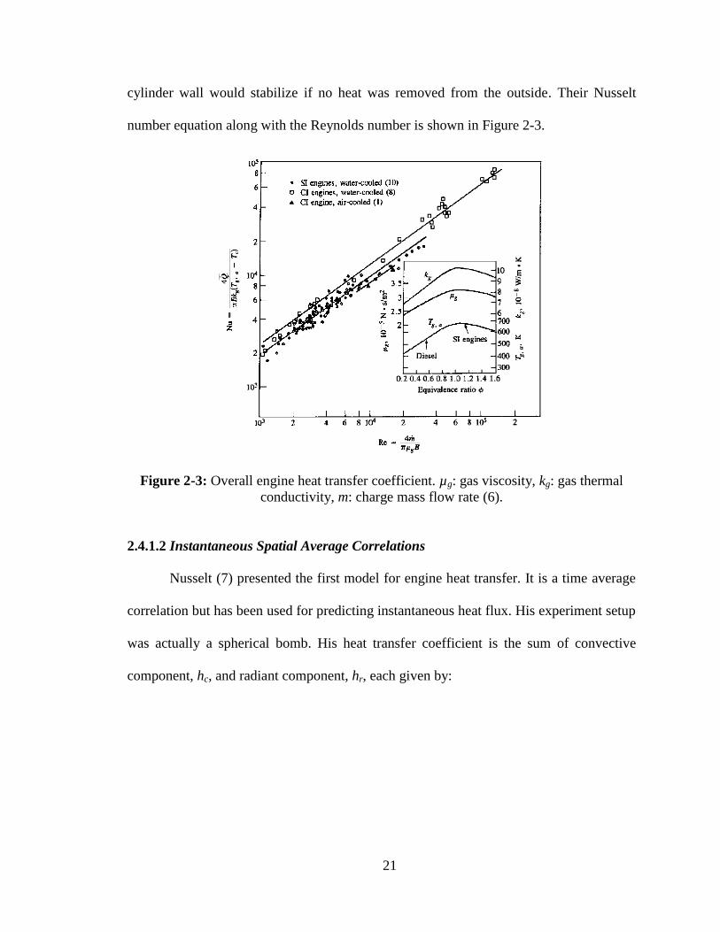
21
cylinder wall would stabilize if no heat was removed from the outside. Their Nusselt
number equation along with the Reynolds number is shown in Figure 2-3.
Figure 2-3: Overall engine heat transfer coefficient. µg: gas viscosity, kg: gas thermal
conductivity, m: charge mass flow rate (6).
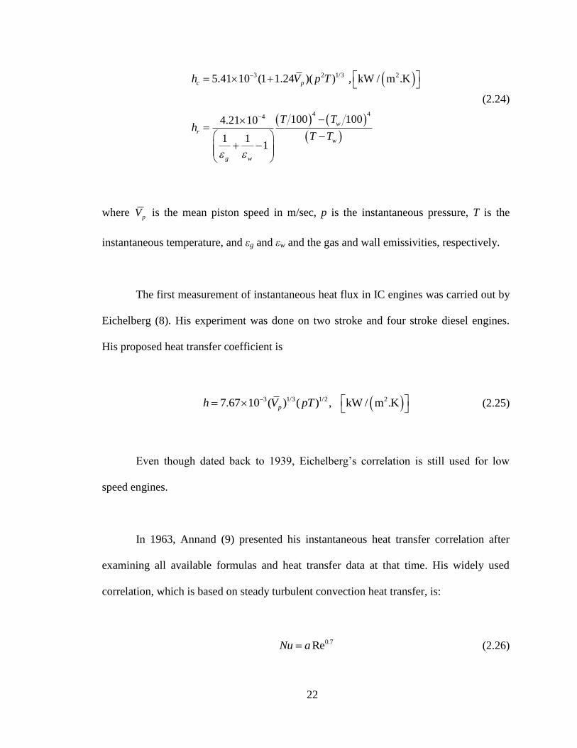
2.4.1.2 Instantaneous Spatial Average Correlations
Nusselt (7) presented the first model for engine heat transfer. It is a time average
correlation but has been used for predicting instantaneous heat flux. His experiment setup
was actually a spherical bomb. His heat transfer coefficient is the sum of convective
component, hc, and radiant component, hr, each given by:
22
3 2 1/3 2
4 44
5.41 10 (1 1.24 )( ) , kW / m .K
100 1004.21 10
1 11
c p
w
r
w
g w
h V p T
T Th
T T
(2.24)
where pV is the mean piston speed in m/sec, p is the instantaneous pressure, T is the
instantaneous temperature, and εg and εw and the gas and wall emissivities, respectively.
The first measurement of instantaneous heat flux in IC engines was carried out by
Eichelberg (8). His experiment was done on two stroke and four stroke diesel engines.
His proposed heat transfer coefficient is
3 1/3 1/2 27.67 10 ( ) ( ) , kW / m .Kph V pT
(2.25)
Even though dated back to 1939, Eichelberg’s correlation is still used for low
speed engines.
In 1963, Annand (9) presented his instantaneous heat transfer correlation after
examining all available formulas and heat transfer data at that time. His widely used
correlation, which is based on steady turbulent convection heat transfer, is:
0.7ReNu a (2.26)

23
where a is a constant whose value depends on the intensity of the charge motion
0.35 0.8a . The characteristic length is the bore and the characteristic velocity is the
piston mean speed. Gas properties are to be evaluated at mean bulk temperature instead
of the average of the gas and wall temperature using the ideal gas law (Equation (2.21)).
Annand full heat flux equation that includes both convection and radiant heat transfer is:
0.7 4 4 2Re ( ) ( ), kW / m w w
kq a T T b T T
B (2.27)
where b = 3.3 x 10⁻¹¹
for diesel engines and 4.3 x 10⁻¹²
for SI engines. Even though data
for this correlation were collected from a thermocouple on the cylinder head, it has been
used as an approximate for instantaneous spatial average heat fluxes for the entire
combustion chamber walls.
Another widely used correlation is the one proposed by Woschni (10). A heat
balance approach was used instead of local temperature measurement to determine the
amount of heat transfer crossing the combustion chamber walls
0.2 0.8 0.8 0.53 20.820 , kW / m .Kh B p W T (2.28)
where W is the average cylinder gas velocity related to the mean piston speed by the
following formula obtained for four stroke, water cooled, four valve diesel engine with
no swirl:
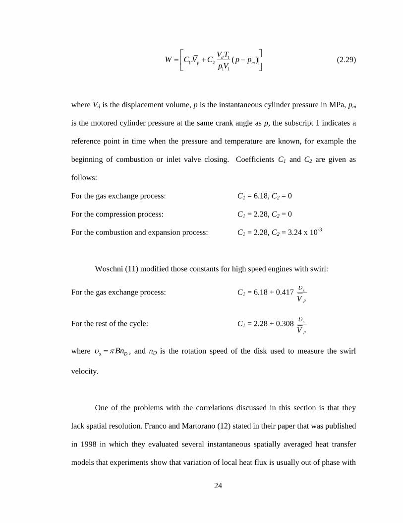
24
11 2
1 1
. ( )dp m
V TW C V C p p
pV
(2.29)
where Vd is the displacement volume, p is the instantaneous cylinder pressure in MPa, pm
is the motored cylinder pressure at the same crank angle as p, the subscript 1 indicates a
reference point in time when the pressure and temperature are known, for example the
beginning of combustion or inlet valve closing. Coefficients C1 and C2 are given as
follows:
For the gas exchange process: C1 = 6.18, C2 = 0
For the compression process: C1 = 2.28, C2 = 0
For the combustion and expansion process: C1 = 2.28, C2 = 3.24 x 10⁻³
Woschni (11) modified those constants for high speed engines with swirl:
For the gas exchange process: C1 = 6.18 + 0.417 s
pV
For the rest of the cycle: C1 = 2.28 + 0.308 s
pV
where s DBn , and nD is the rotation speed of the disk used to measure the swirl
velocity.
One of the problems with the correlations discussed in this section is that they
lack spatial resolution. Franco and Martorano (12) stated in their paper that was published
in 1998 in which they evaluated several instantaneous spatially averaged heat transfer
models that experiments show that variation of local heat flux is usually out of phase with
25
the variation of apparent driving temperature difference between gas and the wall. They
claim that this out of phase behavior is evidence for the variability of heat flux with both
space and time. They further say that “such experimental results have been known for
more than 25 years, but they have been largely ignored.”
In 2005, Schubert et al. (13) mentioned that zero-dimensional models dominate
engine cycle heat transfer simulation due to their simplicity; however, such models do not
yield satisfactory results in certain application because they lack to consider the actual
flow field. Even though this approach gives satisfactory results for a large range of
applications, it became obvious in the last few years that this approach is not suitable for
certain conditions. Example was given on how Woschni’s model predicted too low heat
transfer during intake compared to experiment, causing an over estimate of the
volumetric efficiency values.
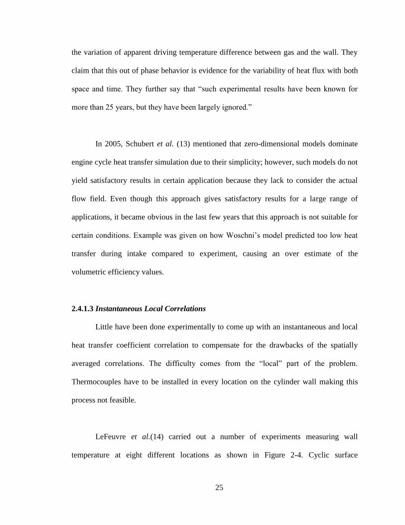
2.4.1.3 Instantaneous Local Correlations
Little have been done experimentally to come up with an instantaneous and local
heat transfer coefficient correlation to compensate for the drawbacks of the spatially
averaged correlations. The difficulty comes from the “local” part of the problem.
Thermocouples have to be installed in every location on the cylinder wall making this
process not feasible.
LeFeuvre et al.(14) carried out a number of experiments measuring wall
temperature at eight different locations as shown in Figure 2-4. Cyclic surface
26
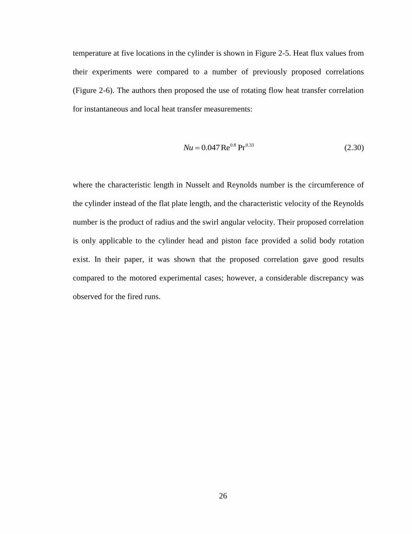
temperature at five locations in the cylinder is shown in Figure 2-5. Heat flux values from
their experiments were compared to a number of previously proposed correlations
(Figure 2-6). The authors then proposed the use of rotating flow heat transfer correlation
for instantaneous and local heat transfer measurements:
0.8 0.330.047Re PrNu (2.30)
where the characteristic length in Nusselt and Reynolds number is the circumference of
the cylinder instead of the flat plate length, and the characteristic velocity of the Reynolds
number is the product of radius and the swirl angular velocity. Their proposed correlation
is only applicable to the cylinder head and piston face provided a solid body rotation
exist. In their paper, it was shown that the proposed correlation gave good results
compared to the motored experimental cases; however, a considerable discrepancy was
observed for the fired runs.

27
Figure 2-4: Thermocouple locations on cylinder head and wall (14).
Figure 2-5: Instantaneous temperature distribution at different locations (14).

28
Figure 2-6: Comparisons of predictions of previous correlations with experimental data
(14).
29
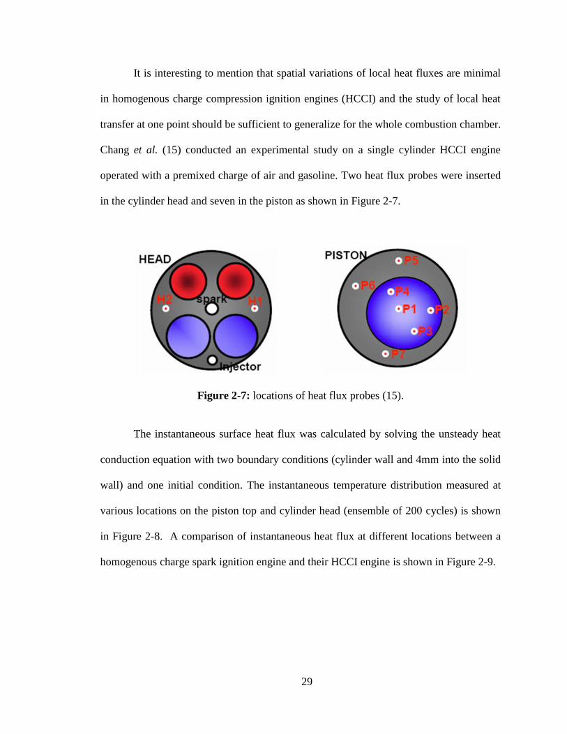
It is interesting to mention that spatial variations of local heat fluxes are minimal
in homogenous charge compression ignition engines (HCCI) and the study of local heat
transfer at one point should be sufficient to generalize for the whole combustion chamber.
Chang et al. (15) conducted an experimental study on a single cylinder HCCI engine
operated with a premixed charge of air and gasoline. Two heat flux probes were inserted
in the cylinder head and seven in the piston as shown in Figure 2-7.
Figure 2-7: locations of heat flux probes (15).
The instantaneous surface heat flux was calculated by solving the unsteady heat
conduction equation with two boundary conditions (cylinder wall and 4mm into the solid
wall) and one initial condition. The instantaneous temperature distribution measured at
various locations on the piston top and cylinder head (ensemble of 200 cycles) is shown
in Figure 2-8. A comparison of instantaneous heat flux at different locations between a
homogenous charge spark ignition engine and their HCCI engine is shown in Figure 2-9.

30
Figure 2-8: Instantaneous temperature distribution measured at various locations on the
piston top and cylinder head (15).
Figure 2-9: Instantaneous heat flux at different locations for a homogenous charge spark
ignition engine (left) and the HCCI engine (right) (15).
The authors explain that the expected heat flux uniformity in HCCI engines is due
to the fact that not only the charge is homogeneous, but also the conditions during
combustion are relatively uniform. Whereas in SI engine, even though having a
homogenous charge, the flame front separates the combustion chamber into a hot burned

31
zone and a cold unburned zone. And in the case of CI combustion, the burning is
heterogeneous that the heat flux measurements indicate the conditions near the heat flux
probe only. Woschni’s equation (Equations (2.28) and (2.29)) was then modified for the
HCCI engine,
0.2 0.8 0.8 0.73
scalingh L p W T (2.31)
121
1 1
. ( )6
dp m
V TCW C V p p
pV
(2.32)
where αscaling is used to tune the coefficient to match engine geometry, and L is the
instantaneous chamber height.
2.4.2 Zonal Models
Zonal model divides the combustion chamber into a number of volumes where
each has its own temperature and heat transfer coefficient. Krieger and Borman (16)
divided the combustion chamber into a burned products and unburned charge zones.
Utilizing Eichelberg correlation, Equation (2.25), a heat transfer coefficient was
determined for each zone.
Borgnakke et al. (17) proposed a local heat transfer two zone model by dividing
the combustion chamber into an adiabatic core and a thermal boundary layer. The
unsteady boundary layer equation was solved for the unburned and burned gas region of
an SI engine. Effective heat conductivity, ke, was modeled in terms of the turbulent

32
kinetic energy and an integral length scale characterized by the k-ε model. The local heat
flux is given by
( ) /e wq k T T (2.33)
where T∞ is the core gas temperature and δ is the boundary layer thickness.
2.4.3 One Dimensional and Three Dimensional CFD Models
Another approach for the heat transfer problem is by solving the one-dimensional
energy equation. Assuming one dimensional heat transfer is acceptable provided that
temperature gradients normal to the combustion chamber wall are much larger than
parallel components.
A number of solutions to the one-dimensional energy equation have been
proposed in the past few decades. Some of the solutions were numerical and assumed
laminar flow. The solutions to the turbulent energy equation often assume “law of the
wall” velocity profile which is not necessarily the case in IC engines.
Three dimensional modeling should provide detailed description of the heat
transfer process in IC engines in addition to velocity, turbulence, and chemical reactions.
One of the major difficulties facing modelers is resolving velocity distribution near the
wall; thus resorting to the “law of the wall” just like the case for the one dimensional
models. The problem with applying this law is that it was originally obtained for two-

33
dimensional, steady, and fully developed flows, and engine flows are far from being
steady and are often three-dimensional motions.
One of the recent computer simulations was by Payri et al. (18) who conducted a
computational study of heat transfer to the walls of a DI diesel engine using commercial
CFD package Fluent. The purpose of the study was to compare their results to, and
modify, a zonal model based on a variant of Woshni equation. The renormalization group
(RNG) k-ε turbulence model was used for closure, with enhanced wall functions.
According to Fluent 6.2 user guide (19), the enhanced wall function is a special
formulation of the law-of-the wall as a single wall law for the entire wall region.

34
CHAPTER 3
FLOW IN THE CYLINDER
Gas flow in the cylinder has a great impact on the performance of the engine. It
has a major role on the combustion process in the engine by enhancing flame speed, and
mixing air and fuel in direct injection engines. Convection heat transfer, which is the
motivation of the research at hand, is another process in which fluid motion has a direct
influence on. Major fluid motions inside the combustion chamber are tumble, swirl, and
squish. Initial forms of tumble and swirl are introduced by the intake process, and then
may break into smaller structures at the end of the intake process or as compression
progresses.
In this chapter, the major fluid motions are described, followed by gas velocity
characteristics (mean and turbulence). A more detailed description of the mean flow
equations is then introduced as a continuation of what briefly discussed in the convection
heat transfer section of the previous chapter (Section 2.3.2) taking into account variable
density, kinetic energy budget, and law of the wall. A literature review for the major
optical diagnostics, namely Laser Doppler Velocimetry (LDV) and Particle Image
Velocimetry (PIV), on IC engines is discussed followed by previous attempts to utilize
those techniques to resolve near-wall velocity.
35
3.1 Major Fluid Motions in the Cylinder
Knowing the major fluid motions, how they are generated, and which part of the
combustion chamber do each one interacts with and for how long, is important to know
before any near wall measurements are carried out. For example, during intake in an off-
axes intake valves, tumble motion is expected to dominate during the intake process, thus
a boundary layer with certain properties influenced by the structure of the free stream
flow is expected to develop along the cylinder head and cylinder walls in the same plane.
If swirl is induced, the free stream behavior would have a different impact on the
development and the shape of the boundary layer at the cylinder wall, cylinder head, and
piston top.
3.1.1 Tumble and Swirl Mean Flows
Tumble and swirl mean flows most of the times coexist; therefore their
descriptions are combined in the same section. Both of these motions are induced in the
cylinder by means of valve lift strategies, and port and valve configurations. Schematic of
both motions are shown in Figure 3-1.

36
Figure 3-1: Schematic of tumble and swirl, Wilson et al. (20).
The intake flow into the cylinder is turbulent and the turbulent velocity is higher
than the mean velocity. The purpose of inducing tumble and/or swirl is to turn the
incoming flow into a coherent flow which is described as an organized mean flow
entrained in the unorganized turbulence. Turbulence in the intake flow is generated by
converting the energy of the incoming flow. This turbulence decays real fast leaving too
little structured motions at ignition. So the purpose of tumble and swirl is to encapsulate
the incoming flow momentum into a coherent flow that is less dissipative and thus lasts
longer. During the compression stroke near top dead center, tumble vortex of the size of
the bore cannot be retained and break up into smaller vortices of the size of the clearance
volume producing high levels of turbulence which produce higher flame speeds.
Inducing tumble/swirl also helps in creating the same large scale from cycle to cycle
which would reduce cycle-to-cycle variability. Other purposes for inducing mean flow
motions are to help having reliable combustion at lean charge or with EGR, and to avoid

37
knock by generating higher flame speed that allow flame to reach end zone before auto-
ignition. Tumble and swirl are also used to stratify the gas inside the cylinder. It is known
that inducing swirl will automatically generate tumble motion, not as intense as the swirl
motion though. Tumble on the other hand can be induced without swirl; however,
secondary tumble motions are usually associated with the main induced mean flow (3).
3.1.2 Squish
Squish occurs toward the end of the compression stroke. Gas flows radially
toward the center of the cylinder as the piston approaches the TDC (Figure 3-2). This
occurs towards the end of the compression stroke and helps in intensifying the swirl
motion.
Figure 3-2: Schematic of how piston motion generates squish (2).
3.2 Mean Velocity and Turbulence Characteristics
As discussed earlier, the flow in the cylinder is turbulent. Turbulent flow is
defined by fluctuations about an average velocity. Therefore, statistical methods are
applied to describe the turbulent flow field. In general, turbulence could be either
38
stationary in which it does not change statistically with time or non-stationary where
statistics vary with time. In cylinder flow is not stationary during the cycle span causing
statistics to be different from one crank angle to another. Due to these differences,
ensemble average is usually used, also called phase average (2). Time average is also
used to find the individual cycle mean, which is also called cycle-resolved mean, which is
usually different in value than the ensemble average mean due to cycle-to-cycle variation.
It is always important to clarify which average is used since it gives different
representation of the cycle mean.
Fluctuation about the mean is used to show the turbulence intensity. It has been a
subject of argument which mean should be used to calculate the turbulence intensity in
engines. In the literature, some use individual cycle time average mean to determine
turbulence intensity and argue that using ensemble average mean will over estimate
turbulence intensity since cycle-to-cycle variation will add up to the fluctuations (21).
They usually call the intensity evaluated at the ensemble average mean “fluctuation
intensity”. Others, however, will calculate turbulence intensity using the ensemble
average mean proposing that cycle-to-cycle variations are mainly due to the initial flow at
the end of the intake process. These differences in flow conditions at the end of the intake
stoke, even if they are small in value, can cause noticeable variability since turbulence is
sensitive to initial conditions (3).
The ensemble average is a function of crank angle θ and individual cycle i. The
instantaneous velocity at a certain crank angle on specific cycle is given by
39
( , ) ( ) ( , )u i u u i (2.34)
where ( , )u i is the fluctuation velocity and ( )u is the ensemble average velocity given
by
1
1( ) ( , )
N
i
u u iN
(2.35)
where N is the number of cycles. The decomposition of an instantaneous property,
whether scalar or vector, into its mean and fluctuation is referred to as the Reynolds
decomposition. The fluctuation/turbulence intensity is defined as the root mean square of
the fluctuation velocity
1/2
2
1
1( , )
N
rms
i
u u iN
(2.36)
The time average, also called cycle-resolved mean, on the other hand is a function
of time t. The instantaneous velocity is given by
( ) ( )u t u u t (2.37)
where ( )u t is the fluctuation velocity and u is the time average velocity given by
40
/2
/2
1( )u u t dt
(2.38)
where η is the time period over which the instantaneous velocity is averaged. It is an
intermediate time scale between the smallest and largest scales of turbulence. The cycle-
resolved mean could also be determined by taking the Fourier transform of the velocity
time record of each cycle. Fourier coefficients of all frequencies above a selected cutoff
frequency are set to zero. The result is inverse transformed back to the time domain
yielding the cycle-resolved mean. This frequency filtering method for determining the
cycle-resolved mean is equivalent to the moving average approach (Equation (2.38)) in
the time domain over a characteristic time interval equivalent to the reciprocal of the
cutoff frequency (22), hence the name “time average”.
3.3 Mean Flow Equations
The mean flow equations were introduced in Chapter 2 with the assumption of
constant density to explain the importance of understanding the flow behavior in order to
solve the convection heat transfer problem properly. The following is a more elaborate
description of mean flow equation taking into account density temporal and spatial
variations.
The continuity equation in index notation is given by
0i
i
ut x
(2.39)

41
The temporal gradient of density cannot be assumed negligible since density
changes drastically throughout the internal engine cycle duration.
Applying Reynolds decomposition and taking the average of Equation (2.39)
results in the following form of the continuity equation:
0i i
i
u ut x
(2.40)
Dividing the terms inside the parenthesis by the mean density leads to the Favre
average of velocity (23),
u
u u
(2.41)
where the first term on the right hand side is the ensemble averaged velocity. Favre
average is actually defined as follows (23)
(2.42)
where θ is any scalar or vector property.
42
If the density is constant per CAD (instantaneous density is equal to the ensemble
averaged density), then the second term in the parenthesis of Equation (2.40) drops out.
Having the same density per realization (CAD) also simplifies calculations of turbulent
quantities where density is involved (i.e. Reynolds stresses).
Therefore, Favre average of the normal x-component Reynolds stresses where
determined from 180 to 330 CAD, and then compared to their corresponding ensemble
averaged values. Error between the two was found to be around 0.31% on average as will
be seen in Chapter 5. Hence, it is reasonable to assume constant density at a given CAD.
The mean continuity equation therefore reduces to
0i
i
ut x
(2.43)
and with mathematical manipulations and with the assumption of spatially homogeneous
density in the combustion chamber, the fluctuation form of the continuity equation
becomes
0i
i
u
x
(2.44)
It is quite important to point out that density cannot be assumed homogenous
within the combustion chamber especially near the wall region because of the substantial
temperature gradient that drives heat transfer to the wall; however, this assumption was

43
made above due to lack of temperature distribution information. This fact should
emphasize the need to carry out a simultaneous thermal boundary layer investigation in
order to have a complete data set that would provide the means for modeling validation.
The Navier-Stokes (momentum) equations are averaged. The result is the mean-
momentum equations, also known as Reynolds equations,
2
i i ij i i j
i j j j
u u upu g u u
t xj x x x x
(2.45)
The Reynolds equations appear to be similar to the Navier-Stokes equations with
the instantaneous velocities and pressure being replaced with their averages. There is,
however, an additional term (4th term on the right hand side of Equation (2.45)). This last
term represents stresses due to turbulent fluctuation motion. These additional stresses are
called apparent stresses or Reynolds stresses.
Analogous to the molecular momentum transport due to viscous stresses,
Reynolds stresses transfer momentum by means of fluctuating velocity field. Davidson
(24) states that Reynolds stresses are not actually true stresses but they represent the
mean momentum fluxes by the turbulence, and the effects of these fluxes can be captured
by pretending that these terms are stresses. Reynolds stresses usually dominate the
viscous stresses; thus, the latter is usually neglected except in regions very close to the
wall.
44
The set of the three Reynolds equations and the continuity equation contain more
than four unknowns. In addition to the average pressure and the three components of the
average velocity, there are also Reynolds stresses which are the components of a second
order tensor. Problem like that is said to be unclosed and additional equations linking the
Reynolds stresses to the mean flow is required to solve the closure problem. These
additional equations are called turbulence models. Brief description on Reynolds stresses
modeling was discussed on the previous chapter.
For this experiment, Reynolds stresses near the cylinder head will be determined
from the 2D vector fields obtained from the μPIV+PTV measurements.
The balance of the kinetic energy of the turbulent fluctuations (k-Equation) is
important when studying turbulence fluctuations and their physical impacts. Equation
(2.46) shows the quantity of the kinetic energy that is to be balanced,
2 21 1
2 2ik q u (2.46)
The k-Equation is given by
212 2
2
ij i j i ij ij ij i j
j j
uDk p u u u u e e e u u
Dt x x
(2.47)
45
The k-Equation illustrates the energy balance between the different inputs of
turbulent fluctuations. The term on the left hand side is turbulence kinetic energy
convection. The first three terms on the right-hand side of represent the diffusion of
turbulent kinetic energy; the first two terms correspond to the diffusion by turbulence,
and the third term denotes viscous diffusion. The fourth term is the turbulent kinetic
energy production which is the rate of energy generation due to the interaction of the
Reynolds stresses with the mean shear. The fifth term on the right-hand side is the
viscous dissipation of turbulent kinetic energy. It is a sink where kinetic energy is
transformed to internal energy.
3.3.1 Boundary Layer Equations for Plane Flows
Following similar assumptions made to laminar boundary layers flows (
, v U x y ), where U∞ is the free stream velocity, the continuity,
momentum, and turbulent kinetic energy equations for plane turbulent boundary layer in
Cartesian coordinates are simplified as follows (for more details on boundary layer
estimations, refer to (25)):
1
0u v
t x y
(2.48)
u u u p u
u v u vt x y x y y
(2.49)
22 2
22
k k k uu v v q k v u v
t x y y y y
(2.50)
46
where the dissipation for plane flows is expanded as follows:
2 22 2
2 2 2u v u v u v
x y y x y x
(2.51)
The velocity fluctuation part of the viscous diffusion (second component in the
second term on the right hand side of Equation (2.50)) is sometimes combined with the
dissipation term resulting in what is known as a pseudo-dissipation. The resulting k-
Equation is
2
2
22
k k k uu v v q k u v
t x y y y y
(2.52)
and the pseudo-dissipation is re-arranged as follows
2 22 2u v u v
x x y y
(2.53)
First order and second order derivatives are determined by finite difference
schemes applied to the vector field grid shown in Figure 3-3.

47
Figure 3-3: Velocity vector grid.
First order and second order spatial derivatives are obtained from the following
two central differences equations, respectively. Spatial derivatives at grid points at the
boundaries are determined by forward and backward differencing the vector field.
Temporal derivatives are obtained similarly. More detailed description of the different
differencing schemes used could be found in (23).
1, 1,
, 2
m n m n
m n
u uu
x x
(2.54)
2
1, , 1,2 2
,
12m n m n m n
m n
uu u u
x x
(2.55)
m,n m+1,n
m,n-1
m,n+1
m-1,n

48
3.3.2 The Universal Law of the Wall
Turbulent flows bounded by at least one solid surface have been investigated for
different types of configurations. Fully developed channel and pipe flows, and the flat
plate boundary layer, in which the mean velocity is mainly parallel to the wall, were
found to have universal characteristics.
Gas flow in internal combustion engines is a unique turbulent wall flow in which
different types of mean motions (tumble, swirl, and squish) are involved throughout the
engine cycle. The flow is primarily three dimensional and the mean flow is not
necessarily parallel to the wall. Flow also varies from one stroke and cycle to another.
While the intake flow exhibits a jet-like flow inducing tumble and/or swirl mean motion,
compression stroke flow is mainly driven by those induced motions. The power stroke
flow is affected by the combustion process and the exhaust stroke gas flow is driven by
pressure difference and piston motion. Valves timing is another factor that impacts the
flow behavior.
With the complexity of the engine gas flow mentioned above, it is important to
study the feasibility of applying the universal law of the wall model, which is derived for
steady and fully developed two dimensional turbulent channel or boundary layer flows, to
the near wall gas flow in internal combustion engines.
In this experiment, the law of the wall will be investigated and compared to
experimental results of near cylinder head flow from 180 to 330 CAD. Results after 330

49
CAD cannot be tested since the flow actually starts decreasing and eventually reversing
as will be shown from the low resolution experiment causing the law of the wall model to
fail. This flow reversal observation emphasizes the need for full optical boundary layer
investigation of the whole engine cycle at different locations to validate or exclude the
application of turbulent model for near wall flows at specific locations and/or timings.
The following is a brief description of the universal law of the wall.
The no-slip boundary condition dictates that the Reynolds stresses are zero at the
wall. The wall shear stress is thus completely due to viscous effects and is equal to:
0
w
y
du
dy
(2.56)
At a given wall shear stress, the inner velocity scale known as friction velocity is
given by
1/2
wu
(2.57)
and the inner (or viscous) length scale is given by
lu
(2.58)

50
The distance from the wall in terms of viscous lengths, known as wall units, is
given by
u yy
yl
(2.59)
which is similar to the friction Reynolds number defined by
Reu
(2.60)
so the magnitude of the wall units could be interpreted as a measure of viscous and
turbulence effects. The inner velocity is given by
u
uu
(2.61)
Based on the wall units, different regions within the turbulent boundary layer are
defined. The inner layer (y/δ < 0.1) is where the average velocity is determined from the
friction velocity (uη) and the wall unit. Within the inner layer is the viscous wall region
(y+ < 50) where the viscous effect on the shear stress is significant, and below y
+ = 5 is
the viscous sublayer where Reynolds shear stress is negligible in comparison with the
viscous stress.

51
In the outer layer (y+ > 50), the effects of viscosity are negligible. The region
between the inner and outer layers is the overlap region (y+ > 50, y/δ < 0.1). Within the
overlap region and the inner layer, the log-law holds between y+ > 30 and y/δ < 0.3. The
region between the viscous sublayer and the log-law region is called the buffer layer (5 <
y+ < 30) (26).
The behavior of the velocity profile within the inner layer is the same whether the
flow is inside a channel or over a flat plate (boundary layer flow). In the outer layer,
however, the boundary layer shows a significant departure from the log law which
requires different treatment of the velocity-defect law which describes the velocity profile
in the outer region (26). In this experiment, the high resolution imaging limits the near-
wall flow investigations to within the inner layer, namely the viscous sublayer and the
log-law region. Therefore, no special assumptions are needed to further approximate the
near cylinder head flow to either a channel flow or a boundary layer (flat plate) flow. It is
important though to have a careful examination to the outer layer region of the near
cylinder head flow in future studies that extend the investigations to a wider range of the
turbulent boundary layer regions.
The viscous sublayer (y+ < 5) velocity profile is linear and given by
u y (2.62)
In the log-law region (y+ > 30 and y/δ < 0.3), the velocity profile is determined by
52
1
lnu y B
(2.63)
where κ is the von Karman constant and is equal to 0.41, and B = 5.2. In the literature,
variations in the values of these two constants are within 5% (26).
3.4 Analysis of Instantaneous Velocity Vector Fields
One of the advantages of two-dimensional velocity vector fields obtained from
PIV is the extended amount of information that could be extracted from the instantaneous
velocity fields. In addition to Reynolds decomposition, which is widely applied to
turbulence statistics as was discussed earlier (i.e. Reynolds stresses and turbulence kinetic
energy budget), other decomposition methods could be used on the instantaneous velocity
fields to reveal more information about the turbulence structure. The visualization and
identification of small-scale structures not only help in assessing the turbulence dynamics
but also extend the analysis of heat transfer problem from studying the mean flow
boundary layer effect to investigating the instantaneous impact of turbulence structures
on transporting thermal energy to and away from the wall.
Adrian et al. (27) explain that identification of vortices in a velocity field and
conducting vortex statistics such as diameter and strength is usually accomplished by
locating regions of isolated regions of significant vorticity. While this procedure is
straightforward in simple flows with minimal shear, vortices in complex flows are
generally masked by region of significant shear which degrades vortex statistics. In such
complex flows, it is difficult to utilize vorticity maps to identify vortices.
53
In addition to Reynolds decomposition, Adrian et al. (27) presents other
decomposition methods that help visualize small-scale structures along with modern eddy
classifier based on critical-point analysis of the local velocity gradient tensor which
determines swirling strength. Those decomposition methods to visualize turbulence
structures and identify their strength are presented next after a brief definition of a vortex.
There is no agreed-upon definition of a vortex. One of the common definitions is
the one by Kline and Robinson (28) in which they state that “A vortex exists when
instantaneous streamlines mapped onto a plane normal to the core exhibit a roughly
circular or spiral pattern, when viewed in a reference frame moving with the center of the
vortex core”.
3.4.1 Visualization of Vortices
From the vortex definition mentioned above, two important conditions should be
met to properly visualize a turbulence structure. The first condition is that a velocity field
must be viewed in a frame that has the same velocity as the vortex core. The second
condition dictates that the vorticity is concentrated at the core of a vortex (27). A
turbulent flow field consists of a number of small-scale structures embedded in a large-
scale structure. To be able to extract those small-scale structures, the velocity at the
center of each small vortex has to be removed.
One of the decomposition methods used to recognize vertical structures is the
Galilean analysis is which the total instantaneous velocity is represented as follows

54
c cu U u
(2.64)
where Uc is a constant convection velocity and uc is the deviation. Most vortical
structures could be revealed if a wide range of convection velocities is tested. Visualized
vortices at a certain convection velocity actually move at that velocity.
Reynolds decomposition (Equation (2.5)) reveals more vortices than a single
Galilean decomposition because vortical structures often move at velocities similar to the
local mean velocity. On the other hand, it removes large-scale features associated with
the mean flow while the Galilean decomposition retains those large-scale structures.
In the large eddy simulation (LES) decomposition, the large-eddy field is defined
by the low-pass filtering the total velocity as follows
, ( , ) ( , )
D
u x t f x x u x t dx
(2.65)
where u is the filtered large-scale field, f is the filtering kernel and D is the domain of the
velocity field. The total velocity field is given by
u u u
(2.66)
where u is the remaining smaller-scale field. The filtering kernel f could be any standard
homogeneous filter (Gaussian, top-hat, etc), or inhomogeneous filter using proper

55
orthogonal decomposition methods (27). Equations (3.31) to (3.33) are adapted from
Adrian et al. (27) where interested reader could refer to for more details on the subject of
vortex visualization.
3.4.2 Vortex Identification
As mentioned earlier, vorticity maps do not show vortex cores only but also
shearing motions in the flow field. Shear layers are highly present in near-wall flows and
relying on the vorticity maps to reveal vortex structures may results in masking out those
turbulent eddies (27). Therefore, other methods have to be applied to extract vortex cores
in order to obtain a more reliable statistics.
One of the methods proposed to identify vortex cores embedded in a flow field is
based on critical-point analysis of the local velocity gradient tensor (29), (30), and (31).
The local velocity gradient tensor (in three dimensions) will have one real eigenvalue (λr)
and a pair of complex conjugate eigenvalues (λcr ± iλci) if the discriminant of its
characteristic equation is positive. Zhou et al. (30) and (31) demonstrate that λci quantifies
the strength of any local swirling motion. Adrian et al. (27) show that for two-
dimensional fields (PIV planar fields), an equivalent two-dimensional form of the local
velocity gradient tensor can be analyzed yielding either two real eigenvalues or a pair of
complex conjugate. Vortices are identified by plotting iso-regions of λci > 0. From
LaVision’s FlowMaster manual (32), λci for a two-dimensional velocity gradient tensor is
given by

56
221 1
2 4ci
u v u v u v
y x x y x y
(2.67)
The plots of swirling strength can be used to validate the results obtained from
flow field decomposition, and to further modify the decomposition parameters to reveal
more vortex motions (i.e. perform local Galilean decomposition in the vicinity of a
vortex, or reduce/increase the size of the LES domain).
3.5 Experimental Flow Diagnostic Techniques and Their Applications to IC Engines
Over the past few decades, laser diagnostic techniques applied to fluid flow
measurements have gained great popularity and became more reliable and accepted as the
laser technology have advanced providing a wide range of products ready to utilize for
different flow measurement situation.
3.5.1 Laser Doppler Velocimetry
Laser Doppler Velocimetry (LDV), also known as Laser Doppler Anemometry
(LDA), was first demonstrated in 1964 by Yeh and Cummins (33). Since then it has
developed into a major non-intrusive flow diagnostic technique that provides
instantaneous velocity and turbulence intensity. LDV can measure velocity at high
temporal resolution at specific spatial locations.
The general setup of LDV consists of a collimated and coherent light source
(laser) that is split into two beams in parallel which then cross each other at the laser

57
beam waist at a certain angle to create straight fringes perpendicular to the flow direction.
The flow is seeded with a material that is light enough to follow the flow faithfully. As
the seeding particles cross the fringes they reflect light to a photo detector. Knowing the
distance between the fringes and the frequency the particles cross the fringes determined
by the photo detector, the velocity can them be calculated.
Early applications of LDV on IC engines were carried out by Witze in the late
1970’s. One of his early papers is (34) where several new measurement techniques were
applied to direct injection stratified charge motored engine. Velocity and turbulence
levels were measured during compression and injection using dual beam backscatter
optical arrangements. Radial distribution of the mean tangential velocity at half of the
clearance height is shown on Figure 3-4. The outermost radial position where velocity
was resolved was at x/R = 0.99 corresponding to 380µm. Radial velocity at this
outermost position ranges 13 to 24 m/s depending on the crank angle as could be seen on
Figure 3-4. The authors concluded that there was no evidence of the wall boundary layer
and it was clearly very thin.
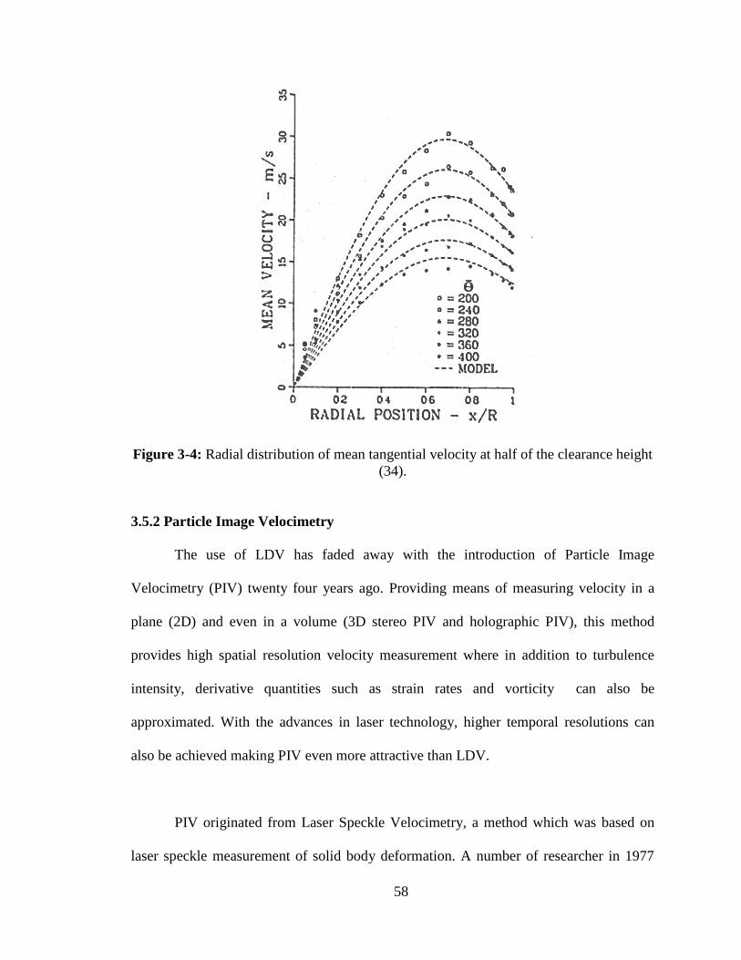
58
Figure 3-4: Radial distribution of mean tangential velocity at half of the clearance height
(34).
3.5.2 Particle Image Velocimetry
The use of LDV has faded away with the introduction of Particle Image
Velocimetry (PIV) twenty four years ago. Providing means of measuring velocity in a
plane (2D) and even in a volume (3D stereo PIV and holographic PIV), this method
provides high spatial resolution velocity measurement where in addition to turbulence
intensity, derivative quantities such as strain rates and vorticity can also be
approximated. With the advances in laser technology, higher temporal resolutions can
also be achieved making PIV even more attractive than LDV.
PIV originated from Laser Speckle Velocimetry, a method which was based on
laser speckle measurement of solid body deformation. A number of researcher in 1977
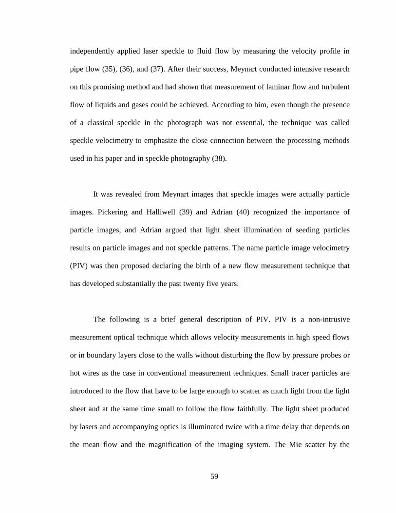
59
independently applied laser speckle to fluid flow by measuring the velocity profile in
pipe flow (35), (36), and (37). After their success, Meynart conducted intensive research
on this promising method and had shown that measurement of laminar flow and turbulent
flow of liquids and gases could be achieved. According to him, even though the presence
of a classical speckle in the photograph was not essential, the technique was called
speckle velocimetry to emphasize the close connection between the processing methods
used in his paper and in speckle photography (38).
It was revealed from Meynart images that speckle images were actually particle
images. Pickering and Halliwell (39) and Adrian (40) recognized the importance of
particle images, and Adrian argued that light sheet illumination of seeding particles
results on particle images and not speckle patterns. The name particle image velocimetry
(PIV) was then proposed declaring the birth of a new flow measurement technique that
has developed substantially the past twenty five years.
The following is a brief general description of PIV. PIV is a non-intrusive
measurement optical technique which allows velocity measurements in high speed flows
or in boundary layers close to the walls without disturbing the flow by pressure probes or
hot wires as the case in conventional measurement techniques. Small tracer particles are
introduced to the flow that have to be large enough to scatter as much light from the light
sheet and at the same time small to follow the flow faithfully. The light sheet produced
by lasers and accompanying optics is illuminated twice with a time delay that depends on
the mean flow and the magnification of the imaging system. The Mie scatter by the
60
seeding particles is recorded by film camera or high-resolution digital camera. The latter
is used in the current research where the output of the camera sensor is transferred
directly from the camera’s built-in memory to the computer memory. Consecutive
particle images are either recorded on the same frame where autocorrelation is used to
process the images or on double frames where cross-correlation is applied to process the
data. Autocorrelation has a drawback of vector direction ambiguity. Image shifting
techniques are used to remove this ambiguity. In digital PIV, each image is divided into
small areas called interrogation windows. Local displacement of the images of the
seeding particles of the first and second illumination is determined for each interrogation
window by statistical method (correlations mentioned above). Velocity vector fields are
then computed provided the knowledge of the calculated displacement and the time delay
between images (41).
The first application of PIV in IC engines was in 1989 by Reuss et al. (42).
Velocity measurements were made in the clearance volume parallel to the piston using a
double-pulsed laser sheet with 20-40 µs pulse separation. Images of the seeded flow were
taken at CA 78 BTDC compression and CA 12 ATDC. Computed velocity fields were
valid to within 500 µm of a surface. Out-of-plane vorticity components were evaluated at
each point in the vector field by computing the circulation around a closed contour
surrounding the point. The authors used this method instead of the first-order difference
scheme to provide smoothing of the vorticity field. Three components of the strain rate
tensor were evaluated from the first-order differences of the vector field at each point.
61
3.6 Literature Review on Near-Wall Velocity Measurements on IC Engines and the
Structures of Turbulent Boundary Layer
Hall and Bracco (21) conducted LDV velocity and turbulence measurements near
the cylinder wall of a non-firing and firing SI engine cycles operating with a swirl
number of 4. The engine was fired every seventh cycle. Tangential velocity
measurements were made in both firing and non-firing cycles at nine spatial locations
with the closest being 0.5 mm from the cylinder wall. Radial velocity measurements were
made at four of the nine locations with the closest component being 1.5 mm from the
cylinder wall (Figure 3-5). Velocity measurements were made at the center of the
clearance height (6.5 cm below the engine head.) in a single-cylinder research engine at
operating speed of 1200 rpm. All measurements were made with one crank angle
resolution from 42 degrees BTDC to 22 degrees ATDC. The seeding particles used were
1.5 µm diameter zirconium oxide (ZrO2) which has good visibility in the burned gas and
minimal window fouling; however, it was found to be abrasive.
Figure 3-5: LDV measurement locations in the center of the clearance height (21).

62
Figure 3-6 shows the tangential ensemble averaged mean velocities in non-firing
cycles at the nine radial locations for a number of crank angles near TDC. The flow
exhibit a solid-body rotation until 1 cm from the wall where velocity decreases due to
momentum diffusion to the wall. Boundary layer is evident as close as 0.5 mm to the
wall. Figure 3-7 shows the tangential ensemble averaged mean velocities in firing cycles
at the nine radial locations for a number of crank angles near TDC. The profiles are more
complicated the non-firing case. There is noticeable increase in tangential velocity ahead
of the flame at crank angles 350 and 355, and then a decrease as the flame passes before
recovering due to the momentum of the swirling flow. The boundary layer is very thin in
both the burned and unburned gas.
Figure 3-6: (left) Ensemble averaged mean velocity profiles measured in non-firing
cycles, (right) Magnified view From Figure 3.5 (21).

63
Figure 3-7: (left) Ensemble averaged mean velocity profiles measured in firing cycles,
(right) Magnified view From Figure 3.6 (21).
Foster and Witze (43) carried out LDV velocity and turbulence measurements
near the engine head wall in SI research engine. A special design toroidal contoured
engine head with the apex at the half the radius of the cylinder was used to make it
possible to get the LDV volume within 60 µm from the wall (Figure 3-8). Two levels of
swirl were used to vary the flow Reynolds number. Boundary layer thickness less than
200 µm was observed in the high swirl motored operation case, and a boundary layer
thickness of 700-1000 µm was noticed for the low swirl motored operation case. The
boundary layer thickness increased when the engine was fired for both levels of swirl.
Engine speed was 300 rpm and it was fired every fifth cycle. Velocity measurements 2
mm below the apex were made. These values were used as the characteristic free stream
velocities to evaluate the Reynolds number with the radial position r as the characteristic
length.

64
Figure 3-8: Schematic of the engine combustion chamber (43).
Figure 3-9 shows the velocity profiles in both the non-firing and the firing cycles
of the high swirl case. For the non-firing cycles (top part of the Figure) the boundary
layer effect could not be observed to within 70µm of the wall. However, velocity
reduction starting 200µm from the wall is noticed after TDC. In the firing cycles (bottom
part of the Figure), only measurements of the burned gas are shown. Measurements as
close to 100µm were obtained; however, the authors suggest that these measurements at
this distance should be discounted because of the erratic behavior mainly caused by beam
steering. The boundary layer thickness increases after combustion is complete due to the
drop in Reynolds number by a factor of more than three between pre-flame and post-
flame flows.

65
Figure 3-10 shows the velocity profiles in both the non-firing and the firing cycles
of the low swirl case. In the non-firing cycles, the boundary layer grows from 200µm to
1000µm during expansion as the outer flow stabilizes. The Y-axis is shifted for the firing
case to account for the negative velocities recorded. The authors explain that since it is
hard to justify negative velocities while the free stream is positive, they believe that beam
steering is again causing problems.
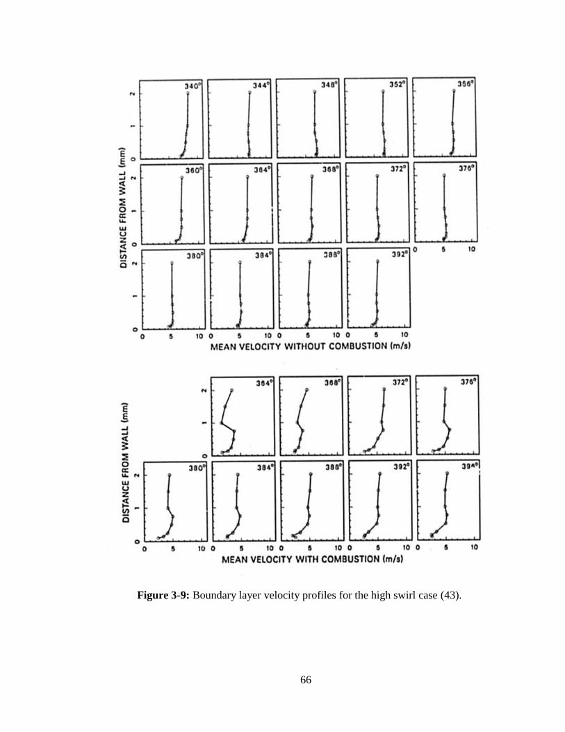
66
Figure 3-9: Boundary layer velocity profiles for the high swirl case (43).

67
Figure 3-10: Boundary layer velocity profiles for the low swirl case (43).
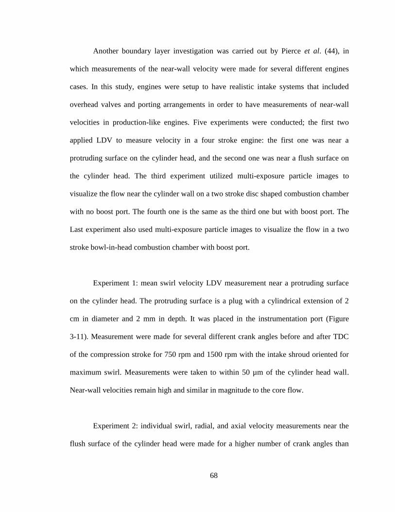
68
Another boundary layer investigation was carried out by Pierce et al. (44), in
which measurements of the near-wall velocity were made for several different engines
cases. In this study, engines were setup to have realistic intake systems that included
overhead valves and porting arrangements in order to have measurements of near-wall
velocities in production-like engines. Five experiments were conducted; the first two
applied LDV to measure velocity in a four stroke engine: the first one was near a
protruding surface on the cylinder head, and the second one was near a flush surface on
the cylinder head. The third experiment utilized multi-exposure particle images to
visualize the flow near the cylinder wall on a two stroke disc shaped combustion chamber
with no boost port. The fourth one is the same as the third one but with boost port. The
Last experiment also used multi-exposure particle images to visualize the flow in a two
stroke bowl-in-head combustion chamber with boost port.
Experiment 1: mean swirl velocity LDV measurement near a protruding surface
on the cylinder head. The protruding surface is a plug with a cylindrical extension of 2
cm in diameter and 2 mm in depth. It was placed in the instrumentation port (Figure
3-11). Measurement were made for several different crank angles before and after TDC
of the compression stroke for 750 rpm and 1500 rpm with the intake shroud oriented for
maximum swirl. Measurements were taken to within 50 µm of the cylinder head wall.
Near-wall velocities remain high and similar in magnitude to the core flow.
Experiment 2: individual swirl, radial, and axial velocity measurements near the
flush surface of the cylinder head were made for a higher number of crank angles than
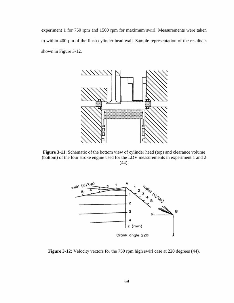
69
experiment 1 for 750 rpm and 1500 rpm for maximum swirl. Measurements were taken
to within 400 µm of the flush cylinder head wall. Sample representation of the results is
shown in Figure 3-12.
Figure 3-11: Schematic of the bottom view of cylinder head (top) and clearance volume
(bottom) of the four stroke engine used for the LDV measurements in experiment 1 and 2
(44).
Figure 3-12: Velocity vectors for the 750 rpm high swirl case at 220 degrees (44).

70
Experiments 3, 4, and 5: Multi-exposure particle pictures were used as the
primary technique used for flow diagnostics. Imaging plane was at half of the height of
the clearance volume. Porting geometry and field of view for experiments 3 through 5 are
shown in Figure 3-13. The boost port shown on the figure was not implemented on
experiment 3 engine. Schematics of engine heads used for each of the three experiments
are shown in Figure 3-14.
Figure 3-13: Porting geometry and field of view for experiment 3 (no boost port,
M=0.83 and M=1.0), experiment 4 and 5 (with boost port, M=1) (44).
Figure 3-14: Schematic of head detail of the combustion chamber for experiment 3 (left),
experiment 4 (left portion of the image on right), and experiment 5 (left portion of the
image on right) (44).
71
The authors stated that the flow visualization results from experiment 3 show that
the existence of well defined boundary layers in engines may be the unusual case.
Rotational structures apparently persist all the way to the cylinder wall. Images were
taken with five laser pulses at TDC with magnification of 0.833 and pulse separation of
80 µs, and at 25 degrees ATDC with magnification of unity and pulse separation of 120
µs. Engine speed in both cases was 750 rpm.
Experiment 4 was run at 500 rpm. Images were taken at TDC with a
magnification of unity, varying only pulse separation timing from 80 µs to 120 µs. The
engine used is similar to the one from experiment 3 with one modification of a boost port.
It was concluded from these two runs that no organized mean flow was apparent and it
only seemed as a decaying turbulent flow. The authors suggest that with the boost port,
no typical boundary layer formation would be expected, and the transport of momentum,
energy, and mass near the wall would be governed by the near-wall turbulent structures
and their interaction with the wall.
Experiment 5 was run at 500 rpm. Images were taken at TDC with a
magnification of unity and pulse separation of 120 µs. The same crank case was used
with the addition of a bowl in the cylinder head to induce squish. The existence of an
eddy right next to the wall surface was noticed.
It could be concluded from Pierce et al. (44) and Foster and Witze (43) that while
LDV measurements can resolve boundary layers in IC engines are quite effective, they
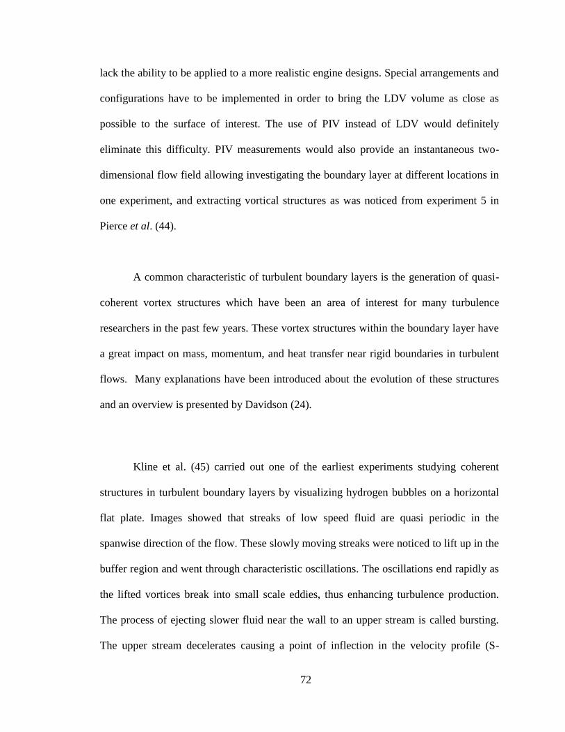
72
lack the ability to be applied to a more realistic engine designs. Special arrangements and
configurations have to be implemented in order to bring the LDV volume as close as
possible to the surface of interest. The use of PIV instead of LDV would definitely
eliminate this difficulty. PIV measurements would also provide an instantaneous two-
dimensional flow field allowing investigating the boundary layer at different locations in
one experiment, and extracting vortical structures as was noticed from experiment 5 in
Pierce et al. (44).
A common characteristic of turbulent boundary layers is the generation of quasi-
coherent vortex structures which have been an area of interest for many turbulence
researchers in the past few years. These vortex structures within the boundary layer have
a great impact on mass, momentum, and heat transfer near rigid boundaries in turbulent
flows. Many explanations have been introduced about the evolution of these structures
and an overview is presented by Davidson (24).
Kline et al. (45) carried out one of the earliest experiments studying coherent
structures in turbulent boundary layers by visualizing hydrogen bubbles on a horizontal
flat plate. Images showed that streaks of low speed fluid are quasi periodic in the
spanwise direction of the flow. These slowly moving streaks were noticed to lift up in the
buffer region and went through characteristic oscillations. The oscillations end rapidly as
the lifted vortices break into small scale eddies, thus enhancing turbulence production.
The process of ejecting slower fluid near the wall to an upper stream is called bursting.
The upper stream decelerates causing a point of inflection in the velocity profile (S-

73
shaped velocity profile). Continuity requires counter flows from high flow layers to occur
toward the wall in other regions; these flows are known as sweeps (26).
Boundary layer structures in steady flows have been the main focus of many
studies, and little has been done on unsteady boundary layers. Costamagna et al. (46) in
their DNS study of coherent structures in oscillatory boundary layers state that
investigating turbulence structures in unsteady accelerating and decelerating flows may
provide additional physical insight regarding the origin and development of wall
turbulence. Furthermore, the study of coherent structures in oscillating or pulsatile flows
is relevant to many science and engineering fields such as biofluid mechanics and
oceanic and atmospheric sciences.
Kearney et al. (47) conducted a time-resolved thermal boundary layer structure
investigation in a pulsatile reversing channel flow to study the impact of flow reversal on
heat transfer from a heated flat plate to a partially and a fully reversing flow. It was found
that in either case the effect of flow reversal was a dramatic thickening of the thermal
boundary layer. They concluded that the main two reasons for the near-wall and bulk
flow increase in temperature were the vertical ejection of fluid from the near-wall region,
a phenomenon encountered in flow reversal, and the limited degree of turbulent
transition. A subsequent dip in temperature following the rapid initial increase was
noticed which was explained by a sudden fluid inrush (sweep) to preserve continuity, as
discussed earlier. The wall heat transfer then recovers as the accelerated boundary layer
flow clears the channel of high enthalpy fluid.

74
While the main purpose of the current research is to study velocity boundary
layers, vortex structures were observed in the vector fields within the boundary layers.
This shows an added benefit for applying μPIV for boundary layer investigations in IC
engines. Future work of sampling vortex structures within the boundary layer could help
in understanding heat transfer in IC engines, in addition to gaining more knowledge about
wall turbulence in unsteady oscillating flows. However, the required high spatial and
temporal resolution for such studies poses particular challenges for such studies in rapidly
varying flows.

75
CHAPTER 4
PIV AND PTV PARAMETER OPTIMIZATIONS AND ERROR ANALYSIS
Following the brief description of PIV presented in section 3.2.2, it is important
now to discuss several parameters that are relevant to PIV and are important in
optimizing the experimental setup and reducing measurement uncertainty.
4.1 PIV Parameters
4.1.1 Imaging System
The imaging system parameters are shown in Figure 4-1. The magnification factor
is determined by
0
0
zM
Z (3.1)
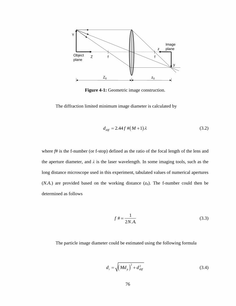
76
Figure 4-1: Geometric image construction.
The diffraction limited minimum image diameter is calculated by
2.44 # 1diffd f M (3.2)
where f# is the f-number (or f-stop) defined as the ratio of the focal length of the lens and
the aperture diameter, and λ is the laser wavelength. In some imaging tools, such as the
long distance microscope used in this experiment, tabulated values of numerical apertures
(N.A.) are provided based on the working distance (z0). The f-number could then be
determined as follows
1
#2 . .
fN A
(3.3)
The particle image diameter could be estimated using the following formula
2
2
p diffd Md d (3.4)
Object
plane
Image
plane
Y
Z
z
y
Z0 z0
f f

77
where dp is the seeding particle diameter. The depth of field is given by
22 # ( 1) /diffz f d M M (3.5)
4.1.2 Particle Image Shift
The flow speed is described by
u X t u (3.6)
where α is the scaling or calibration factor that provides the physical amount of flow
velocity and it is determined via calibration of the camera by simply placing a target with
known spacing in the image plane (laser sheet plane). ΔX is the particle displacement (in
pixels) detected by means of correlating particle patterns of two successive images
separated by a known time interval Δt. δu is the uncertainty in velocity measurements.
The time interval must be optimized such that the maximum particle displacement is not
larger than one quarter the final interrogation window size (48)
1
4IWs d (3.7)
where dIW is the interrogation window size.
The measurement location and time are defined by the following two equations

78
0/ 2s ex X X X (3.8)
/ 2s et t t (3.9)
where X0 is the origin of the image plane, Xs and Xe are the starting and ending position of
the correlation window, ts and te are the first and the second laser pulse time.
4.1.3 Seeding Tracking
To analyze seeding constraints, i.e. evaporation and time response of the droplets
in the flow, the in-cylinder temperatures have to be determined first. Temperature at the
beginning of the compression stroke (180 CAD) is estimated to be equal to the intake air
temperature set at 45 ºC. Pressure is acquired from a transducer located at the cylinder
head that provides reading at every crank angle. Subsequent temperatures are determined
for the compression stroke by applying the following isentropic relation for an ideal gas
1
2 2
1 1
k
kT P
T P
(3.10)
where P is the cylinder pressure provided by the pressure transducer, k is the air specific
heat ratio, and T is the in-cylinder temperature.
The air viscosity is determined from the Sutherland law (49) given by

79
3/2
T SuT
T T Su
(3.11)
where μ is viscosity, μo is a reference value equal to 1.716E-5 N.s/m2 for air, To is a
reference temperature of 273 K for air, Su is the Sutherland constant and it has a value of
111 K for air.
The time response of the seeding particles is determined from
2
18
p p
p
a
d
(3.12)
where ρp is the seeding particles density, dp is their diameter, and μa is the air viscosity
calculated using Equation (3.11). The seeding particles time response shall be compared
with a number of time scales to determine how realistically those tracers follow the
engine gas flow. The following analysis is adapted from (50).
The engine time scale is found by applying the following equation
e
p
S
V (3.13)
where S is the engine stroke and pV is the piston mean speed. The engine time scale, τe,
describes the effect of time varying boundary conditions on the flow variation rate.

80
The turbulent turn-over time scale is given by
t
rms
L
u
(3.14)
where L is the length scale of the most energetic eddies, u´rms is the fluctuation intensity
defined as the root mean square of the fluctuation velocity (see section: Mean Velocity
and Turbulence Characteristics). Following the analogy of Lumley (3), L is estimated to
be 1/6 the largest possible eddy which is approximated to be the clearance height, and
u´rms is approximated to be the piston mean speed for the first half of the compression
stroke, and half the piston mean speed for the second half of the compression stroke.
The resolved eddies turn-over time scale is given by
2/3
tL
(3.15)
where Δ is twice the final grid spacing of the applied algorithm and must be above
estimates of ~10 µm for the Kolmogorov scale in engines (3).
Engine time scale, turbulent turn-over time scale, and resolved eddies turn-over
time scale should be compared to the time response of the seeding particles by means of
the Stokes number given by

81
p
St
(3.16)
where η is the corresponding time scale, i.e. engine time scale, turbulent turn-over time
scale, and resolved eddies turn-over time scale.
4.1.4 Particle Image Density
Optimum seeding density is required when conducting a PIV experiment in order
to obtain a high valid detection rate and a low measurement uncertainty. Keane and
Adrian (48) and (51) in their Monte Carlo simulations recommend that the seeding
density should be optimized to produce 15 or more particle images per interrogation spot.
Megerle et al. (52) experimentally investigated the effect of particle image counts
among other factors (i.e. f-stop, magnification, and focusing) on the accuracy and
precision of digital PIV. A minimum RMS error of 2% was obtained for particle image
count of 10 within a 32x32 interrogation window. Higher seeding counts did not seem to
give an advantage regarding accuracy since the measured fluctuations of the particle
images displacements were found to be independent in the range of 10-40 particle images
within the 32x32 interrogation window.
A major difficulty in conducting μPIV is meeting the optimum particle image
count (~10 image particles per interrogation window). One of the recommended solutions
for low seeding density is to process the data applying an ensemble averaged correlation
(32), or overlaying a number of raw (unprocessed) images to produce one image with
82
higher density (41). While the first option seems plausible, it only produces and ensemble
averaged flow field, thus losing a lot of valuable statistics and the ability to calculate
different turbulent terms. The second option on the other hand seems reasonable to be
used if the flow under investigation is laminar.
The third option is combining PIV and PTV in a hybrid scheme where PIV serves
as a predictor of the flow field and the PTV algorithm corrects for it. The predictor PIV
algorithm could use larger interrogation window size (i.e. 64x64 pixels) to increase the
number of seeding particles by a factor of 4, thus increasing the valid detection rate and
decreasing measurement uncertainty. The PTV algorithm then tracks individual particles
between the two images with the guidance of the PIV predicted flow filed. More
description of the hybrid algorithm is provided in the data processing section of Chapter
5.
4.2 Error Analysis
In addition to the systematic (bias) error, random error that is due to measurement
uncertainty should also be taken into account.
4.2.1 Systematic Error
Systematic (bias) error is caused by the statistical method of cross-correlation and
the subsequent post-processing schemes. Using different algorithms to process and post-
process PIV images will result in different levels of accuracy (53). In the second
international PIV Challenge (53), the PIV algorithm provided by the LaVision team
(software used in current research to process the PIV images) had a bias error of 0.113
83
pixels when tested for a hundred synthetic images of a turbulent channel flow. The PTV
algorithm provided by LaVision which uses their own PIV scheme as a predictor
performed the best among other PTV team with a bias error of 0.2 pixels. It was noticed
in the challenge that PTV algorithms in general outperformed PIV ones in near wall
velocity analysis due to the reduced effect of the wall bias on the interrogation windows.
4.2.2 Random Errors
Random errors induced by measurements could be evaluated by determining
RMS deviation from the mean. This method cannot be implemented to the results of the
current experiment since the RMS deviation from the mean includes turbulence
fluctuations and cycle to cycle variations. Therefore the sources of measurement
uncertainty shall be investigated by breaking the PIV experimental setup down into sub-
systems and investigating each sub-system for possible errors. Error sources and their
propagation are detected following the recommended procedures and guidelines of the
25th
International Towing Tank Conference (54). Below are the error sources
corresponding to calibration α, displacement of particle image ΔX, time interval Δt, and
seeding velocity lag.
4.2.2.1 Calibration (α)
The calibration is conducted by placing a calibration plate of a known spacing in
the object plane (laser sheet plane) as shown in Figure 4-2. The scaling or calibration
factor (α) (also known as the magnification factor, a term that is not used here to avoid
confusion with the imaging magnification M) is given by

84
1cos, mm / pixelr
r
l
L
(3.17)
where lr is the distance between the reference points on the calibration plate, Lr is the
corresponding distance on the image plane, θ1 is the angle between the light sheet and the
calibration plate.
Figure 4-2: Calibration plate positioning in the laser sheet plane (image plane).
Calibration board: Image distance of reference points Lr
The position of the reference points is determined from single pixel leading to an
uncertainty band of 0.5 pixels. Since two points are involved in determining Lr, the total
uncertainty will be 0.7 pixels. The sensitivity factor (the partial derivative of Equation
(3.17)) is
21
2
cos, mm / pixelr
r r
l
L L
(3.18)
Calibration plate
Laser sheet
lr
θ1
θ2Right angle
View angle
85
Calibration board: Physical distance of reference points lr
The error of the 1.2 mm spaced calibration plate is estimated to be 0.001 mm. The
sensitivity factor of lr is
1cos, 1/ pixel
r rl L
(3.19)
Optical system: Image distortion
Image could be distorted by lens aberration which affects the accuracy of
calibration factor. No data is available for the lenses used in the experiments regarding
their distortion percentage due to aberration. In general, the error will be distortion
percentage times Lr, and the sensitivity factor is the same as Equation (3.18).
Optical system: CMOS distortion
No data is available regarding the amount of distortion of the CMOS chip used.
According to the uncertainty procedure adapted here (54), this error is usually small and
can be neglected.
Experimental condition: Calibration plate position
The difference between the position of the laser sheet and the calibration plate
could affect the accuracy of the measurements. The uncertainty band could be estimated
to be the depth of field (see Equation (3.5)). For the sensitivity factor, the pinhole camera
model is assumed and α could be described as

86
01cosr
r
zl
L f
(3.20)
where z0 is the working distance shown in Figure 4-1, and f is the focal length. The
sensitivity factor will be
1
0 0
cos, 1/ pixelr
r
l
z L z
(3.21)
Experimental condition: Parallel calibration plate
The angle θ1 between the laser sheet and the calibration plate could be estimated
by
1
1 sintotal
z
x
(3.22)
where δz is the depth of field, and xtotal is the width of the field of view. The sensitivity
factor is
1
1
sin, [mm / pixel]r
r
l
L
(3.23)
4.2.2.2 Displacement of Particle Image (ΔX)
Errors due to particle displacement are categorized as follow:

87
Visualization: Laser power fluctuation
The maximum error could be estimated as the seeding particle diameter (1 μm). In
well controlled experimental conditions, error could be reduced to 1/10 of the particle
diameter. Since the displacement is obtained from two particle images, the error band is
estimated as Δx = 0.14 μm, and the sensitivity factor obtained from Equation (3.8) is
1
, pixel / mmX
x
(3.24)
Optical system: Lens and CMOS distortions
Lens and camera chip (CMOS) distortion were discussed earlier on their effect on
calibration. The former was not accounted for due to lack of data, and latter was assumed
negligible.
Optical system: Normal view angle
Deviation from the ideal right angle between the camera setup and the laser sheet
plane (θ2 in Figure 4-2) and its sensitivity factor are estimated in a similar manner as for
θ1.
Data processing
Error inherited from data processing is the systematic error discussed earlier.
88
4.2.2.3 Time Interval (Δt)
The sources of error associated with laser timing are discussed below. The
sensitivity factor for the time measurement is 1.
Delay generator
The high speed controller (HSC) provided by LaVision controls the timing of the
camera and laser. It receives two signals from the engine encoder which are a signal per
cycle (PPC) and a signal per crank angle degree (360°), and outputs triggering signals to
the laser and camera. According to the user manual, the jitter is less than 1 ns.
Laser pulse timing accuracy
The laser used has a 5 ns jitter in pulse timing. The signal to pulse delay is about 3 μs.
4.2.2.4 Seeding Velocity Lag (δu)
The error induced by seeding velocity lag could be estimated from the Stokes
number that corresponds to the turbulent turn-over time scale. Stokes number (in %) is
multiplied by the velocity u to give the uncertainty caused by seeding velocity lag (δu).
The combined uncertainty for each parameter is then calculated using the general
formula for error propagation given by
2 2 2
1 1 2 2 .....c i ic c c (3.25)
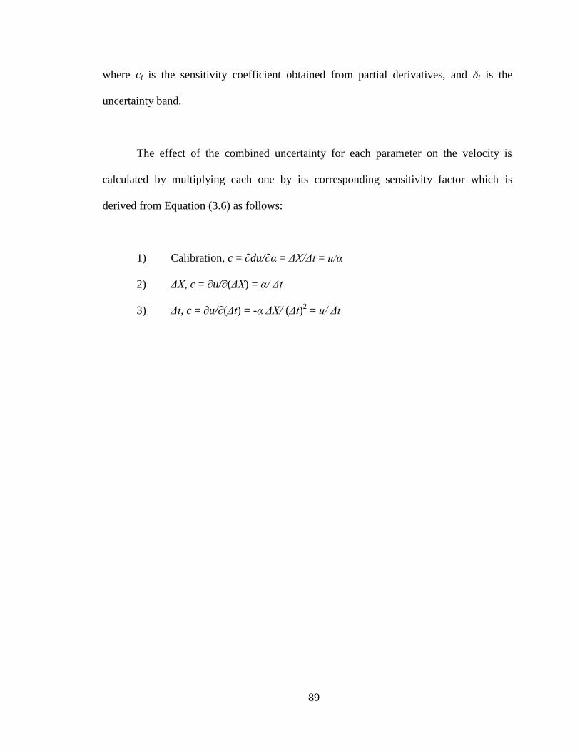
89
where ci is the sensitivity coefficient obtained from partial derivatives, and δi is the
uncertainty band.
The effect of the combined uncertainty for each parameter on the velocity is
calculated by multiplying each one by its corresponding sensitivity factor which is
derived from Equation (3.6) as follows:
1) Calibration, c = ∂du/∂α = ΔX/Δt = u/α
2) ΔX, c = ∂u/∂(ΔX) = α/ Δt
3) Δt, c = ∂u/∂(Δt) = -α ΔX/ (Δt)2 = u/ Δt

90
CHAPTER 5
LOW AND HIGH RESOLUTION PIV EXPERIMENTS NEAR THE CYLINDER
HEAD
This chapter presents high-speed PIV measurements of the boundary layer flow at
a production-type four-valve pent-roof cylinder head of a spark ignition direct injection
engine. Two experiments were conducted; one at a low spatial resolution and high
temporal resolution of 4.8 kHz (imaging at every crank angle) utilizing PIV to get a
general overview of the flow behavior near the cylinder head during the compression and
expansion strokes. In the second experiment, PIV and Particle Tracking Velocimetry
(PTV) were applied to measure two-dimensional near-wall velocity fields at the cylinder
head at 2.4 kHz. To achieve the spatial resolution that is required to resolve important
structures of the boundary layer, a long distance microscope was used to image Mie
scattering signals onto a CMOS camera. Results are reported with a spatial resolution of
45 μm as close as 22 μm from the wall for measurements during the compression and
expansion strokes in a motored engine. This study presents the first step towards a
complete characterization of dynamic boundary layers in internal combustion engines. In
addition to the flow properties, in a second step the temperature distribution in the gas
phase and on the surface will have to be simultaneously measured as well. This can be
achieved with laser-induced fluorescence (55) and phosphorescence imaging (56).

91
5.1 Experiment
5.1.1 Setup
The experiment was conducted in a four-stroke, single cylinder, four-valve spark
ignition direct injection optical engine. The engine head is pent-roof shaped with a spark
plug located on the exhaust valves side and the eight-hole injector located on the intake
valves side oriented in a way that part of the injection is aimed at the spark plug. The
intake system consists of a bulk flow port and a tangential port. The bulk flow port could
be closed to create a high level of swirl rated at 5.5 swirl ratio. In this experiment, the
bulk flow valve was left open providing a 0.8 swirl ratio. Engine specifications are shown
in Table 5.1. The optical components of the engines are transparent quartz cylinder, two
flat quartz windows located at both sides of the pent-roof combustion chamber, and
quartz windows located on the top and sides of the piston (Figure 5-1). For this
experiment, imaging was carried out through the flat pent-roof windows. The field of
view is in the tumble flow plane at the cylinder head between the spark plug and the fuel
injector as shown in Figure 5-1 and Figure 5-2.
Figure 5-1: Schematic of the optical SIDI engine. Field of view shown on the right
image is for the high resolution experiment. The low resolution measurements cover the
entire area between the spark plug and the fuel injector.
2.25 mm
1.69 mm
Fuel Injector Spark Plug
Field of ViewSpark Plug
Fuel
Injector
HEAD
Quartz Top
Window
PISTON
CLAMP PLATE
Quartz Side
Windows
Quartz
Cylinder Light Sheet
Exhaust
Valves
Intake
Valves
Field of View
2.25x1.69 mm

92
Figure 5-2: Light sheet position on the cylinder head between spark plug and injection,
viewed from bottom of the engine (57). Indicated field of view location is for the low
resolution experiment. The high resolution field of view is within the range shown as in
the right of Figure 5-1.
Table 5.1: Optical SIDI engine specifications. Note: valves timings are with 0.1 mm lift.
Connecting Rod 159 mm
Bore 86 mm
Stroke 86 mm
Displacement 500 cm3
Compression Ratio 9.0:1
Intake Valve Open (IVO) 717 CAD
Intake Valve Close (IVC) 231 CAD
Exhaust Valve Open (EVO) 497 CAD
Exhaust Valve Close (EVO) 12 CAD
Engine Speed 800 RPM
Intake Pressure 95 kPa
Intake Temperature 45 ºC
A dual oscillator single head 527 nm Nd:YLF laser (Quantronix Darwin-Duo)
was operated at a frequency of 4.8 kHz and 5.5 mJ/pulse for the low spatial resolution
experiment and at 2.4 kHz and 17 mJ/pulse for the high spatial resolution experiment.
Time separation between laser pulses was optimized to best meet the maximum
44 mmSpark
plug
location
Intake valves
Piston outline
Field of
view
location
xy
z
Fuel injector
location

93
displacement value of 1/4 (or less) the interrogation window size suggested by Keane and
Adrian (48).
Since maximum velocity within the field of view varies throughout the
compression and expansion strokes, variable time separation would be a good feature to
fulfill the maximum displacement value of 1/4 the interrogation window size criterion.
However, with the lack of ability to vary time separation as function of CAD during
image recording, it was chosen to satisfy the maximum displacement for a wide range of
crank angle degrees. Displacement was less than the recommended maximum
displacement for the rest of crank angle degrees intervals which still meets Equation (3.7)
, except for the first four crank angle degrees of the compression stroke where
displacement was higher and on the order of 1/3 of the interrogation window size, which
according to Keane and Adrian (48) represents an upper limit after which the valid
detection rate declines sharply. For the low resolution experiment with a final
interrogation window of 32x32 pixels and pulse separation of 35 μs, the displacement
was between 6 to 8 pixels for most of the compression stroke and 2 to 5 for the expansion
stroke before the exhaust valves open. A maximum displacement of 12 pixels was
recorded at the beginning of the compression stroke. For the high resolution µPIV+PTV
experiment with a final PIV interrogation window of 64x64 pixels and pulse separation
of 15 μs, the displacement was between 6 to 16 pixels for most of the compression stroke
and 4 to 10 for the expansion stroke before the exhaust valves open. A maximum
displacement of 20 pixels was recorded at the beginning of the compression stroke.

94
Imaging through thick windows can lead to aberrations that limit the use of PIV in
engines (58). Static imaging tests through the 18 mm thick, flat side window in the
cylinder head produced high quality Mie scattering images from the seed droplets, even
when using the long distance microscope. For the low resolution experiment, a 105 mm
1:2.8D lens (Sigma DG Macro) was used to image Mie scattering signals onto the camera
chip. The f-number was set to 11. For the high resolution μPIV experiment, a long
distance microscope (Questar Corporation QM 100) was used to collect the Mie
scattering. The long distance microscope has a working distance ranging from 150 mm to
380 mm. In this experiment, it was set at a distance of 190 mm which gave a numerical
aperture NA = 0.128. The f-number was then determined from Equation (3.3) to be 3.9.
For both experiments, the camera was calibrated using a mm-spaced resolution target
giving a calibration factor of 21.43 µm/pixel and a magnification M = 1 for the low
resolution experiment and a calibration factor of 2.82 µm/pixel and a magnification M =
7.8 for the high resolution experiment. The PIV velocity measurements for the low
resolution experiment based on a 32x32 interrogation window with 50% overlap
produced a vector every 343 µm and the PIV+PTV velocity measurements for the high
resolution experiment based on a 64x64 interrogation window with 50% overlap for the
PIV part and a final 16x16 grid reconstruction after the PTV part produced a vector every
45 µm.
Details of the experimental setup are shown in Figure 5-3. Laser beams were
reflected by a HR532 45º mirror and then passed through a telescope to expand them into

95
laser sheets. The two overlapping light sheets were reflected upward by a 45º mirror
sending the light sheet through the piston top window to illuminate the tumble plane.
Figure 5-3: A) HR532 mirror, B) telescope lens, C) 45º mirror, D) long distance
microscope.
A summary of the PIV parameters is shown in Table 5.2.
Table 5.2: PIV parameters.
Parameter Low Resolution High Resolution
Light sheet thickness 1 mm 1 mm
Field of view 9.94x10.63 mm2 2.25x1.69 mm
2
Magnification 1.0 7.8
f-number 11 3.9
Depth of field 1.25 mm 50 µm
Vector spacing (16x16
grid spacing) 343 µm 45 µm
Heat resistant, high flash point, low volatility phenylmethyl polysiloxane silicone
oil droplets (Dow Corning® 510) as PIV seeding were produced using one jet of a six-jet
atomizer (TSI Model 9306). The seeding density was controlled via a pressure regulator
attached to the atomizer and the droplet stream was added to the combustion chamber
Dual Oscillator
Nd:YLF Laser
C
B
D
A
CMOScamera

96
through the intake plenum. Mie scattering signals from the seeding particles were
recorded by a high-speed 14-bit CMOS camera (Vision Research Phantom 7.3) equipped
with 16 GB onboard memory. At 2.4 kHz, the camera could use the full chip with
800x600 pixels.
Seeding constraints analysis, i.e. evaporation and time response of the droplets in
the flow, was performed following the procedure shown in Chapter 4, section 1 (Equation
(3.10) to Equation (3.16)). Temperature at the beginning of the compression stroke (180
CAD) was estimated to be equal to the intake air temperature set at 45 ºC. Pressure was
acquired from a transducer located at the cylinder head that provides reading at every
crank angle. A maximum temperature of 456 ºC was determined at 357 CAD. From the
silicone oil manufacturer specifications, the autoignition temperature is estimated to be
482 ºC and the percentage of volatile content by weight after 4 hours at 250 ºC is 2.5 at
atmospheric pressure. These figures rule out significant evaporation of the seed droplets.
This was confirmed during preliminary tests where strong Mie scattering images were
obtained throughout the expansion stroke, after the droplets were already exposed to the
highest in-cylinder temperature.
Table 5.3 shows the different time scales at different crank angle degrees. Engine
time scale, turbulent turn-over time scale, and resolved eddies turn-over time scale were
compared to the time response of the seeding particles by means of the Stokes number
(Equation (3.16)).

97
Table 5.3: Particle time scale, flow time scales, and the corresponding Stokes number as
a function of CAD.
τp (s) τe (s) Ste τt (s) Stt τΔ (s) StΔ
180
CAD 2.85x10
-6 3.76x10
-2 7.60x10
-5 7.04x10
-3 4.05x10
-4 2.22x10
-4 1.29x10
-2
225
CAD 2.79x10
-6 3.76x10
-2 7.42x10
-5 6.34x10
-3 4.40x10
-4 2.14x10
-4 1.30x10
-2
270
CAD 2.45x10
-6 3.76x10
-2 6.54x10
-5 4.34x10
-3 5.65x10
-4 1.89x10
-4 1.30x10
-2
315
CAD 1.95x10
-6 3.76x10
-2 5.19x10
-5 3.82x10
-3 5.10x10
-4 2.87x10
-4 6.80x10
-3
360
CAD 1.61x10
-6 3.76x10
-2 4.29x10
-5 1.56x10
-3 1.03x10
-3 2.13x10
-4 7.57x10
-3
5.1.2 Data Acquisition
The lasers and camera were synchronized via a USB high-speed controller (HSC,
LaVision). The controller receives a signal each crank angle degree from the engine
encoder, and a signal every cycle (720 degrees) from a hall-effect sensor. Double frame
images with time separation of 35 μs for the low resolution experiment and 15μs for the
high resolution experiment one were recorded. For the low resolution PIV experiment,
images were recorded every crank angle degree during the compression and expansion
strokes from 180 CAD to 489 CAD with 360 being TDC compression. For the high
resolution PIV and PTV experiment, images were obtained every other crank angle
degree during the compression and expansion strokes from crank angle 180 to 540. It
should be noted that the high resolution results will only be shown from 180 to 490 CAD
because the high velocity increase once the outlet valves opened made velocity
calculations impossible with the minimum possible time delay between the lasers
provided by the high speed controller.

98
At the beginning of each run, images were recorded with the laser sheet only (no
seeding) for ten cycles. These unseeded images were then averaged and used to
determine a threshold level for the local noise intensity coming from the camera chip and
the bright reflections from solid objects, which in current experiment were mostly
reflections off the cylinder head. Those reflections were reduced prior to the experiment
by applying a flat black paint (Krylon® Short Cuts
® paint pen) at the boundary of interest.
This helped reducing the intensity of the cylinder head glare by 84%. The average
intensity of the high resolution background is 600 counts, for the low resolution
measurement it is 300 counts compared to a dynamic range of the camera of 16,384
counts (14 bit).
5.1.3 Data Processing
Double-frame images were processed using commercial software (LaVision
Davis 7.2). In addition to the background subtraction described in the previous paragraph,
other pre-processing procedures were applied to further filter out noise. Beside the
common noise of camera chip and bright reflections from solid objects, which are usually
encountered in PIV, a stationary fixed fringe pattern was a dominant source of noise in
the high resolution experiment. By investigating the experiment setup components by a
process of elimination, it is believed that the camera chip is the source of this fringe.
Monochromatic light can cause a fringe pattern produced by the interference between
light waves that reflects within the CMOS chip creating what is known as Newton’s rings
(59). A batch operation was executed on each crank angle series to calculate the
minimum intensity value at all pixel positions. Then this pixel-specific minimum is

99
subtracted from all images in the series. A stationary fixed pattern such as the fringe
intensity adds to the particle images intensities, and the minimum intensity value at a
certain position is the background intensity of the fringe intensity when no particle
intensity is added to the background. Since the seeding density is low enough,
statistically, this procedure effectively eliminates the fringe pattern. Then a non-linear
sliding minimum filter of pixel size 10 was used before cross-correlating the double
frame images. This high pass filter removes the local mean background intensity (over a
scale of the specified number of pixels) leaving only the local fluctuations, i.e. the
smaller-sized particle images that were on the order of 8 pixels in diameter.
The evaluation of PIV images requires sufficient seeding density, typically 8-10
seeding particles per interrogation window, in order to obtain reliable and accurate
results. Seeding density was sufficient for the low resolution experiment; however,
seeding density is usually low in μPIV and here also due to the proximity of the surface.
In the high resolution experiment, seeding density was 1 to 3 particles per a 32x32
interrogation window. An alternative to using a PIV algorithm for low density images is
particle tracking velocimetry (PTV) where velocity is determined by tracking individual
particles.
A hybrid PIV+PTV method was applied to evaluate the double frame images
obtained in the high resolution experiment. The evaluation starts with a standard PIV
algorithm to determine a “predictor” velocity field. PIV vector field computations were
processed starting with a 128x128 pixel interrogation window and decreased by half to a

100
final size of 64x64 pixels instead of the 32x32 pixels intended for the PIV evaluation
only in the case of the low resolution experiment; the 50% window overlap was
maintained. With the new larger window size, the seeding count is 4 to 12 particles per
interrogation window, hence increasing the reliability of the PIV calculations, keeping in
mind that gradients within the increased interrogation window might have an effect on
the velocity vector value. However, since the PIV results are used as a predictor-only for
PTV, the window size will not have an impact on the accuracy of the final velocity field.
A standard deviation filter was applied to remove spurious vectors and a mean of
adjacent vectors was used to replace those vectors. The resolution of the vector field was
then further refined by detecting and tracking individual particles by the PTV algorithm,
which increases the number of vectors per PIV interrogation window from one to the
total number of particles per same window. The particle detection method adapted in
DaVis looks for the position of the highest intensity and arranges an interrogation
window (not to be confused with the PIV interrogation window) of the size of the particle
diameter around the position of the maximum intensity. The PTV interrogation window
in the second frame is shifted by the “predictor” vector from the PIV calculations.
Finally, an individual particle correlation will correlate the intensity pattern of both
windows to determine the exact shift. The same post processing median filter applied to
the PIV results was also applied to the PTV results. A final step of converting the vector
field to a 16x16 pixel grid was then applied using a second order polynomial fit (60) and
(32).
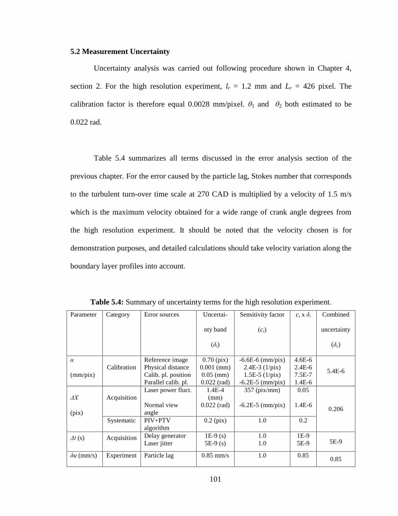
101
5.2 Measurement Uncertainty
Uncertainty analysis was carried out following procedure shown in Chapter 4,
section 2. For the high resolution experiment, lr = 1.2 mm and Lr = 426 pixel. The
calibration factor is therefore equal 0.0028 mm/pixel. θ1 and θ2 both estimated to be
0.022 rad.
Table 5.4 summarizes all terms discussed in the error analysis section of the
previous chapter. For the error caused by the particle lag, Stokes number that corresponds
to the turbulent turn-over time scale at 270 CAD is multiplied by a velocity of 1.5 m/s
which is the maximum velocity obtained for a wide range of crank angle degrees from
the high resolution experiment. It should be noted that the velocity chosen is for
demonstration purposes, and detailed calculations should take velocity variation along the
boundary layer profiles into account.
Table 5.4: Summary of uncertainty terms for the high resolution experiment.
Parameter Category Error sources Uncertai-
nty band
(δi)
Sensitivity factor
(ci)
ci x δi Combined
uncertainty
(δc)
α
(mm/pix)
Calibration
Reference image
Physical distance
Calib. pl. position
Parallel calib. pl.
0.70 (pix)
0.001 (mm)
0.05 (mm)
0.022 (rad)
-6.6E-6 (mm/pix)
2.4E-3 (1/pix)
1.5E-5 (1/pix)
-6.2E-5 (mm/pix)
4.6E-6
2.4E-6
7.5E-7
1.4E-6
5.4E-6
ΔX
(pix)
Acquisition
Laser power fluct.
Normal view
angle
1.4E-4
(mm)
0.022 (rad)
357 (pix/mm)
-6.2E-5 (mm/pix)
0.05
1.4E-6 0.206
Systematic PIV+PTV
algorithm
0.2 (pix) 1.0 0.2
Δt (s) Acquisition Delay generator
Laser jitter
1E-9 (s)
5E-9 (s)
1.0
1.0
1E-9
5E-9 5E-9
δu (mm/s) Experiment Particle lag 0.85 mm/s 1.0 0.85 0.85
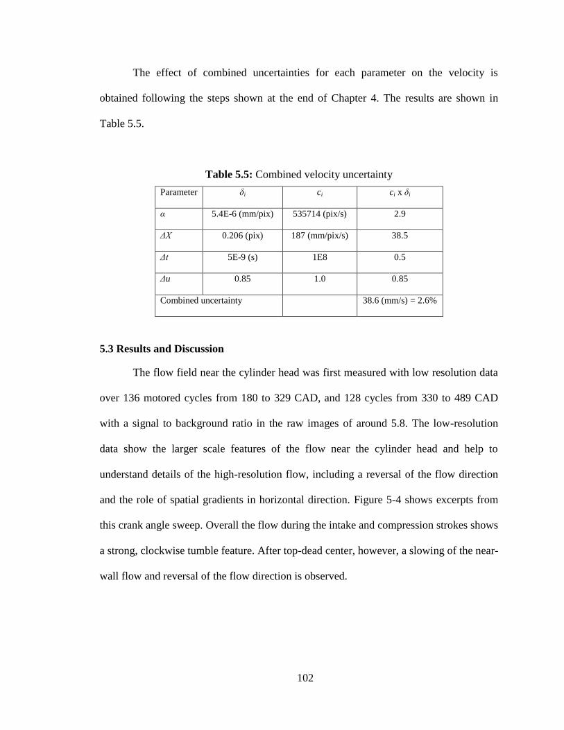
102
The effect of combined uncertainties for each parameter on the velocity is
obtained following the steps shown at the end of Chapter 4. The results are shown in
Table 5.5.
Table 5.5: Combined velocity uncertainty
Parameter δi ci ci x δi
α 5.4E-6 (mm/pix) 535714 (pix/s) 2.9
ΔX 0.206 (pix) 187 (mm/pix/s) 38.5
Δt 5E-9 (s) 1E8 0.5
Δu 0.85 1.0 0.85
Combined uncertainty 38.6 (mm/s) = 2.6%
5.3 Results and Discussion
The flow field near the cylinder head was first measured with low resolution data
over 136 motored cycles from 180 to 329 CAD, and 128 cycles from 330 to 489 CAD
with a signal to background ratio in the raw images of around 5.8. The low-resolution
data show the larger scale features of the flow near the cylinder head and help to
understand details of the high-resolution flow, including a reversal of the flow direction
and the role of spatial gradients in horizontal direction. Figure 5-4 shows excerpts from
this crank angle sweep. Overall the flow during the intake and compression strokes shows
a strong, clockwise tumble feature. After top-dead center, however, a slowing of the near-
wall flow and reversal of the flow direction is observed.
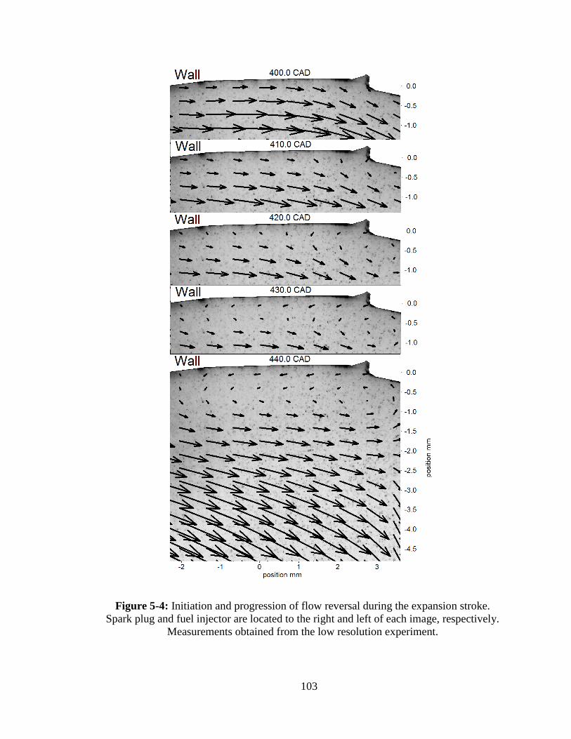
103
Figure 5-4: Initiation and progression of flow reversal during the expansion stroke.
Spark plug and fuel injector are located to the right and left of each image, respectively.
Measurements obtained from the low resolution experiment.

104
Velocity gradients in horizontal direction are noticed in Figure 5-4. Therefore,
care must be taken when conducting high magnification imaging experiments near the
cylinder wall to avoid shift in the field of view. A simple act such as tightening a bolt on
the camera-lens fixture moves the field of view drastically (in a micro-imaging sense),
which could result in different outcomes.
5.3.1 Mean Velocity and Fluctuation Intensity Profiles
An example averaged velocity field measured with high resolution is shown in
Figure 5-5. This field of view was covered using the full resolution of the CMOS chip at
800 x 600 pixels. The origin of the y-axis is at cylinder head and the distance from the
cylinder wall to the first measured vector is approximately 22 μm. The gray background
in Figure 5-5 shows a typical raw image obtained at high resolution with a signal to
background ratio of around 1.7.
Figure 5-5: Ensemble-averaged velocity vector fields for crank angle 180. The
highlighted area shows the region from where the horizontal (x-) velocity component of
seven adjacent vertical profiles are spatially averaged and then are used for further
analysis. Shown in the background is a raw image of seeded flow. Note that for clarity in
this image only every fourth vector in each direction is displayed to allow visualization of
the vector tip.
y
x

105
For this high-resolution experiment, data rates near the surface are low since the
seeding density is lower than in the free stream. Therefore, to improve the statistical
significance of the results, the horizontal (x-) velocity component of seven adjacent high-
resolution ensemble-averaged vertical velocity profiles were averaged for this study.
Their respective normalized standard deviation was used to show that spatially averaging
over a small width of 315 μm that is spanned by the seven vertical high-resolution
velocity profiles does not bias the results. This is shown in Table 5.6, where this
normalized standard deviation remains well below 5% except for the points closest to the
surface. Figure 5-6 shows all seven individual velocity profiles at 180 CAD to illustrate
the negligible spatial velocity gradient in the horizontal direction.
Table 5.6: Standard deviation of seven adjacent horizontal velocity components as a
function of distance from the wall for selected CAD.
Standard Deviation/Average Velocity (%)
y-location (mm) 180 CAD 270 CAD 360 CAD 450 CAD
0.045 23.8 19.3 14.4 30.0
.675 1.0 1.5 3.8 0.6
1.35 0.8 0.8 1.9 4.6
Figure 5-6: Seven velocity profiles were used to determine a spatially averaged (over
315 μm) velocity profile to improve the statistical significance of the velocity data closest
to the surface. The example shown was taken at 180 CAD and shows the low variation
across the averaged region, justifying this approach.
0.0
0.2
0.4
0.6
0.8
1.0
1.2
1.4
0 0.5 1 1.5 2 2.5
Dis
tan
ce
Fro
m W
all (m
m)
Mean Velocity (m/s)
180 CAD
106
Ensemble-averaged velocity vector fields and the fluctuation intensities for the
high-resolution data were calculated from data measured for 98 consecutive motored
cycles from 180 to 490 CAD at every other crank angle. Figure 5-7 shows the evolution
of the ensemble-averaged high resolution profiles of the horizontal velocity component
during the engine cycle and, for more details, Figure 5-8 shows velocity profiles at
selected crank angles for the duration of compression and most of the expansion stroke.
Velocity is highest at the beginning of the compression stroke because both intake valves
are still open. The primary (bulk flow port) intake valve and the secondary (tangential
port) intake valve start closing at 110 and 112 CAD, respectively. Velocity decreases as
the primary and secondary intake valves close until they are fully closed at 231 and 242
CAD, respectively. The maximum velocity from 240 to 290 CAD remains around 1 m/s.
In this region, the momentum brought into the combustion chamber by the intake flow is
dissipating; however, it is compensated for by the momentum gained from the upward
piston movement. After 290 CAD, velocity starts increasing until 330 CAD.
Figure 5-7: Ensemble-averaged velocity profile as a function of crank angle during the
compression stroke and most of the expansion stroke (180 to 490 CAD).
0.0450.5851.125
-2.10
-1.05
0.00
1.05
2.10
180 220 260 300 340 380 420 460
Me
an
Ve
locity (m
/s)
Crank Angle

107
Figure 5-8: Ensemble-averaged velocity profiles at selected CAD during the end of the
compression stroke and most of the expansion stroke.
Around 330 CAD, velocity starts to decrease as the piston slows down when it
approaches TDC. The mean tumble flow breaks down to structures of the size of the
clearance height, which results in a loss of flow momentum. Flow velocity continues to
gradually decrease until around 400 CAD when a flow recirculation in the opposite
direction of the mean in the vicinity of the spark plug initiates flow reversal near the wall
region while the region away from the wall continues in the same direction with no
reversal. This is more prominently visible in the low-resolution vector fields shown in
Figure 5-4 that shows the progress of the flow reversal, initiated by a recirculating flow
0.0
0.2
0.4
0.6
0.8
1.0
1.2
1.4
-1 -0.5 0 0.5 1 1.5 2 2.5
Dis
tance F
rom
Wall
(mm
)
Mean Velocity (m/s)
CA 180
CA 210
CA 240
CA 270
CA 300
0.0
0.2
0.4
0.6
0.8
1.0
1.2
1.4
-1 -0.5 0 0.5 1 1.5 2 2.5
Dis
tance F
rom
Wall
(mm
)
Mean Velocity (m/s)
CA 330
CA 360
CA 390
CA 420
CA 450
108
next to the spark plug. This near wall reversal then extends to cover the wall area
between the spark plug and the fuel injector, while the region away from the wall still
maintain its original flow direction. At 489 CAD, the whole flow field reverses direction
because of the blow down stream into the cylinder when the exhaust valves start lifting.
This is because the exhaust backpressure is several kPa above the in-cylinder pressure at
the exhaust valve opening. It should be noted that while the specified exhaust valve
opening (EVO) is at 497 CAD at 0.1 mm lift, they actually start lifting at 489 CAD.
In-cylinder flows in general exhibit strong variability (3). High fluctuation
intensities were also measured in the engine used in this study (57) and (61). The profiles
showing the horizontal fluctuation intensity component confirms that this is also the case
in the near-wall flow region (Figure 5-9). Fluctuation intensities are on the order of the
mean velocities throughout the engine cycle.

109
Figure 5-9: Fluctuation intensity profile as a function of crank angle (180 to 450 CAD).
5.3.2 Vortex Visualization and Identification
The capability to conduct an extensive vortex structure investigation in
combustion chambers should complement the study of velocity boundary layers to better
understand the engine heat transfer problem. The application of PIV to study boundary
layers in internal combustion engines has the added benefit of visualizing and identifying
near wall vortex structures from the instantaneous flow fields. This addition broadens the
study of engine heat transfer from investigating mean velocity profiles and their impact
on the energy equation to exploring the effect of vortical structures embedded in the
0.0
0.2
0.4
0.6
0.8
1.0
1.2
1.4
0 0.5 1 1.5 2 2.5
Dis
tance F
rom
Wall
(mm
)
Fluctuation Intensity (m/s)
CA 180
CA 210
CA 240
CA 270
CA 300
0.0
0.2
0.4
0.6
0.8
1.0
1.2
1.4
0 0.5 1 1.5 2 2.5
Dis
tance F
rom
Wall
(mm
)
Fluctuation Intensity (m/s)
CA 330
CA 360
CA 390
CA 420
CA 450

110
instantaneous flow fields in transporting momentum and energy from and away from the
wall.
Low and high resolution instantaneous velocity vector fields were analyzed
applying different decomposition methods. Figure 5-10 shows a low resolution
instantaneous velocity vector field (sub-figure: a) decomposed using different methods.
Sub-figures b to e show different results applying Galilean decomposition (deviation
velocity field, uc: see Equation (3.31)). The maximum velocity of the ensemble averaged
velocity field, Umax,mean was used as a basis to vary the convection velocity, Uc. For sub-
figures b, c, and d, the convection velocity is 0.7 Umax,mean, 0.5 Umax,mean, and 0.3
Umax,mean, respectively. For sub-figure e, the convection velocity used was the spatial
average of the instantaneous velocity vector field (spatial average of sub-figure a). As
discussed in Chapter 3.4.1, most vortical structures could be revealed if a wide range of
convection velocities is tested. The Galilean decomposition is sometimes preferred
because it retains the mean flow motion. Reynolds decomposition is primarily applied to
analyze turbulence statistics (i.e. turbulence intensity, Reynolds stresses, and kinetic
energy budget). The fluctuation velocity vector field, u´, is shown in sub-figure f.
Reynolds decomposition reveals more vortices than any single Galilean decomposition
because vortical structures often move at velocities similar to the local mean velocity. On
the other hand, it removes large-scale features associated with the mean flow. Sub-figure
g represents the small-scale structures revealed by a high-pass LES filter. It is noted that
this filter is capable of extracting more structures than either the Galilean or the Reynolds
decomposition methods. This is expected since the high-pass filter in general is the

111
instantaneous flow field minus the low-pass filter where velocities are averaged over a
local domain where its size represents filtering cut-off scale . So instead of subtracting a
constant convection velocity as in the Galilean decomposition, or an ensemble average as
in the Reynolds decomposition, the LES high-pass filter subtracts a local convection
velocity averaged over a predetermined domain, thus removing slowly changing
background in space. In sub-figure f, the averaging domain was chosen to be of the size
of 1 mm (3 grid spacing). This domain size was chosen based on the swirling strength
map that will be discussed next where the average noticeable vortex structure was on the
order of 1-2 mm. The LES domain size could be reduced or increased to visualize
structures of smaller or larger sizes, respectively. Sub-figure g shows the low-pass LES
filter which was subtracted from the instantaneous velocity vector field to obtain the
high-pass filter.
Vortex identification based on critical-point analysis of the local velocity gradient
tensor (see Chapter 3.4.2) was applied to the instantaneous velocity vector fields. The
maps of swirling strength help identify the location, size, and strength of vortical
structures. Those maps also help in verifying or modifying flow visualization methods.
For example, by comparing the swirling strength map to the Galilean decomposed flow
field, one can change the convection velocity values to an equivalent of the local velocity
averages within the area occupied by each individual identified vortex. While this seems
to be a tedious procedure, it would definitely help visualize all possible structure sizes
while retaining the mean flow behavior. In the case of LES filtering, the size of the

112
domain where the filter is applied could be varied to resolve smaller or larger scales
depending on what the swirling strength map is revealing.
The swirling strength maps obtained from the instantaneous flow field of Figure
5-10 (sub-figure a) is superimposed to each decomposed flow field shown in same figure,
except the low-pass LES (sub-figure h). Results are shown in Figure 5-11. It could be
seen that the Galilean decomposed fields need several convection velocities to reveal all
possible vortical structures. While the Reynolds decomposed field reveals more
structures than any of the Galilean decomposed fields, there are still some identified
structures that are not visible in the decomposed vector field. For this flow field, LES
decomposition seems to show all possible vortices except for a number of small ones
which require domain size smaller than the 3 grid spacing used (minimum possible is 2
grid spacing). The effect of changing the domain of the LES filter will be discussed next
when examining the high resolution results.

113
Figure 5-10: a) Low resolution instantaneous flow field decomposed using a number of
Galilean convection velocities: b) Uc = 0.7 the maximum velocity of the ensemble
averaged flow field (Umax,mean), c) Uc= 0.5 Umax,mean, d) Uc = 0.3 Umax.mean, e) Uc =
instantaneous velocity field spatial average, f) Reynolds decomposition, g) high pass
LES, h) low pass LES.
a: instantaneous vel. field b: Galilean, Uc= 0.7 Umax,mean c: Galilean, Uc= 0.5 Umax,mean
f: Reynolds decomposition
g: high-pass LES h: low-pass LES
d: Galilean, Uc= 0.3 Umax,mean e: Galilean, Uc= spatial avg.
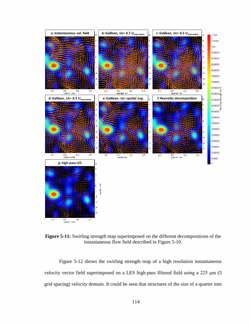
114
Figure 5-11: Swirling strength map superimposed on the different decompositions of the
instantaneous flow field described in Figure 5-10.
Figure 5-12 shows the swirling strength map of a high resolution instantaneous
velocity vector field superimposed on a LES high-pass filtered field using a 225 μm (5
grid spacing) velocity domain. It could be seen that structures of the size of a quarter mm
a: instantaneous vel. field b: Galilean, Uc= 0.7 Umax,mean c: Galilean, Uc= 0.5 Umax,mean
d: Galilean, Uc= 0.3 Umax,mean e: Galilean, Uc= spatial avg. f: Reynolds decomposition
g: high-pass LES

115
are revealed with this LES size domain, there are still some smaller size structures shown
on the swirling strength map that are not extracted with this LES domain size. Figure
5-13 shows a swirling strength map superimposed on a LES filtered field applying a 225
μm domain (top) and a 90 μm domain (2 grid spacing). By comparing the LES
decomposed fields to the swirling strength map, the high-pass LES filter applying the 90
μm domain reveals more smaller-scale structures.
Figure 5-12: High resolution instantaneous velocity vector field decomposed using high
pass LES filter applied over a 0.225 mm domain (5 grid spacing).

116
Figure 5-13: High resolution instantaneous velocity vector field decomposed using high
pass LES filter applied over a 225 μm domain (5 grid spacing) (top image) and a 90 μm
domain (2 grid spacing) (bottom image).
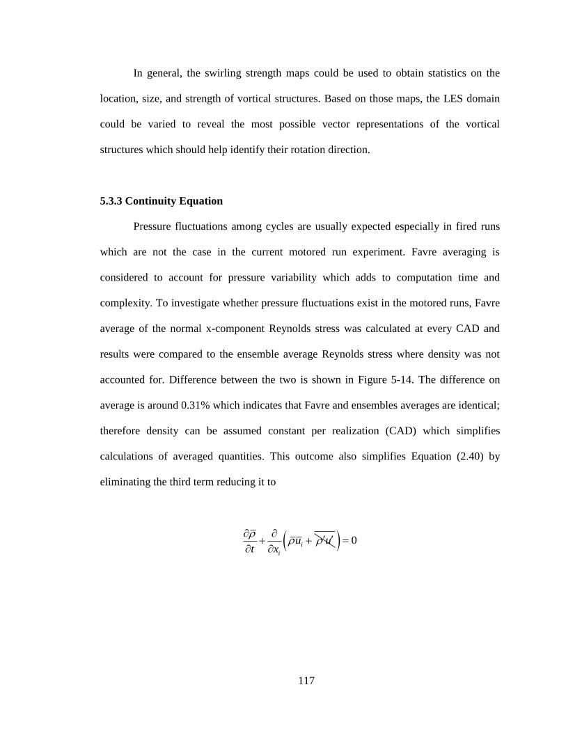
117
In general, the swirling strength maps could be used to obtain statistics on the
location, size, and strength of vortical structures. Based on those maps, the LES domain
could be varied to reveal the most possible vector representations of the vortical
structures which should help identify their rotation direction.
5.3.3 Continuity Equation
Pressure fluctuations among cycles are usually expected especially in fired runs
which are not the case in the current motored run experiment. Favre averaging is
considered to account for pressure variability which adds to computation time and
complexity. To investigate whether pressure fluctuations exist in the motored runs, Favre
average of the normal x-component Reynolds stress was calculated at every CAD and
results were compared to the ensemble average Reynolds stress where density was not
accounted for. Difference between the two is shown in Figure 5-14. The difference on
average is around 0.31% which indicates that Favre and ensembles averages are identical;
therefore density can be assumed constant per realization (CAD) which simplifies
calculations of averaged quantities. This outcome also simplifies Equation (2.40) by
eliminating the third term reducing it to
i
i
u ut x
0
118
Figure 5-14: Difference between Favre averages and ensemble averages.
Continuity equation is expanded and re-arranged to check for the in-plane motion
(z-component). For lack of information, spatial gradients of density are not accounted for;
however, their importance on balancing the continuity equation shall be pointed out in the
following discussion.
1 1w u v
u v wz t x y x y z
The density temporal gradient (first term on the right hand side) is calculated
using central differencing in time. Velocity gradients (second and third term on the right
hand side) are determined by central differencing in space. A plot of the density term and
the combined velocity gradients, which is the divergence, versus the crank angle degrees
is shown in Figure 5-15.
0.0
0.2
0.4
0.6
0.8
1.0
1.2
1.4
1.6
1.8
2.0
180 210 240 270 300 330 360
(Favre
Avg -
Avg)/
Favre
Avg*1
00
CAD
Rexx Difference (%)

119
Figure 5-15: Divergence and temporal density gradient versus CAD.
If the flow is two dimensional, the two terms shown in Figure 5-15 must sum up
to zero. It is obvious from the discrepancy between the two that there is a noticeable out
of plane motion at the measurement plane throughout the compression stroke. Engine
flows in general are three dimensional and the extent of the magnitude of the out of plane
velocity component depends on a number of factors such as combustion chamber design,
and swirl and tumble levels. In the current engine under investigation, the field of view is
in the tumble plane and there is a swirl flow of a ratio of 0.8 induced by the intake
manifold configuration, which would definitely have an impact on promoting a third
velocity component in the tumble plane flow.
The spark plug which is located few millimeters downstream also has an impact
on promoting a third velocity component in the out of plane direction as illustrated in
Figure 5-16.
-400
-300
-200
-100
0
100
200
300
400
500
600
700
180 230 280 330
(1/s
)
CAD
du/dx+dv/dy 1/ρ[d/dt(ρ)]

120
Figure 5-16: Spark plug impact on enhancing the third velocity (z-) component.
Another important factor that might had an effect on the balancing of the
continuity equation was ignoring the density spatial gradients, which if neglected in the x
and z directions only could be acceptable but not in the y direction (normal to the
cylinder head). Maximum gas core temperature in the combustion chamber in a motored
run at 800 RPM was estimated to reach 730 K which is more than twice the cylinder head
temperature approximated at the coolant temperature of 318 K. This indicates that there
must be a significant density gradient in the normal to the wall direction (y-axis). This
density gradient should have an opposite sign of the u velocity gradient since the density
is expected to increase as the cold wall is approached; hence, impact balance of the
continuity equation.
Divergence of the ensemble averaged velocity vector fields was determined to
detect any possible temperature gradient which would vary the density within the velocity
profile. The divergence images shown in Figure 5-17 do not indicate any gradients in
either direction. Therefore, most of the imbalance of the continuity equation could be
xy
z
Spark plug

121
caused by a third velocity component (in-plane z-component) due to the swirl motion and
the presence of the spark plug which is located few millimeters downstream.
Figure 5-17: Divergence of the ensemble averaged velocity fields at selected CAD.
5.3.4 The Law of the Wall
The law of the wall was constructed based on the inner velocity and length scales
(Equations (2.57) and (2.58)). Fluid properties (viscosity and density) were evaluated at
the wall temperature approximated to the coolant temperature of 95° C. Finding the inner
122
velocity length scale actually depends on the knowledge of the wall shear stress which in
turn is based on the mean velocity gradient (du/dy) at the wall (y = 0). The mean velocity
gradient was approximated by dividing the mean velocity closest to the wall by its
corresponding distance from the wall, which could be within 45 μm. It was hard to
determine the exact location of the wall after preprocessing the raw PIV images
(background subtraction, subtracting sliding minimum, and subtracting pixel-specific
ensemble minimum). The viscous sublayer (u+ = y
+) was used as a criterion to determine
the exact distance of the closest measured velocity to the wall. Different values for the
distance from the wall (y in Equation (3.23)) were tested (22.5 μm, 33.75 μm , and 45
μm). The value of 22.5 μm gave the best results among the three suggested values in
terms of the closest fit between the viscous sublayer of the constructed law of the wall
and the experimental velocity profiles. The mean velocity profiles and the distance from
the wall were normalized by the inner velocity and length scales giving u+ and wall units
y+. In addition, viscous sublayer and log-law velocity profiles were calculated using
Equations (2.62) and (2.63), respectively. Normalized experimental velocity profiles
compared to viscous sublayer and log-law for selected crank angle degrees are shown in
Figure 5-18.
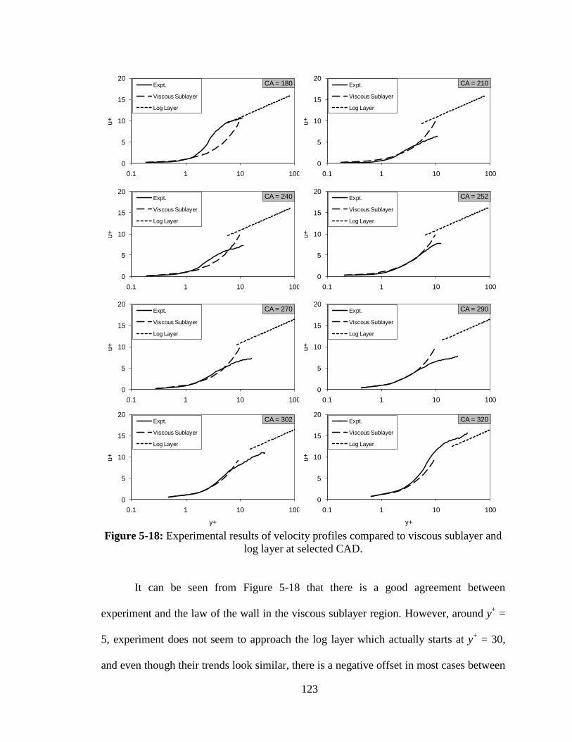
123
Figure 5-18: Experimental results of velocity profiles compared to viscous sublayer and
log layer at selected CAD.
It can be seen from Figure 5-18 that there is a good agreement between
experiment and the law of the wall in the viscous sublayer region. However, around y+ =
5, experiment does not seem to approach the log layer which actually starts at y+ = 30,
and even though their trends look similar, there is a negative offset in most cases between
0
5
10
15
20
0.1 1 10 100
u+
y+
CA = 180Expt.
Viscous Sublayer
Log Layer
0
5
10
15
20
0.1 1 10 100
u+
y+
CA = 210Expt.
Viscous Sublayer
Log Layer
0
5
10
15
20
0.1 1 10 100
u+
y+
CA = 240Expt.
Viscous Sublayer
Log Layer
0
5
10
15
20
0.1 1 10 100
u+
y+
CA = 252Expt.
Viscous Sublayer
Log Layer
0
5
10
15
20
0.1 1 10 100
u+
y+
CA = 270Expt.
Viscous Sublayer
Log Layer
0
5
10
15
20
0.1 1 10 100
u+
y+
CA = 290Expt.
Viscous Sublayer
Log Layer
0
5
10
15
20
0.1 1 10 100
u+
y+
CA = 302Expt.
Viscous Sublayer
Log Layer
0
5
10
15
20
0.1 1 10 100
u+
y+
CA = 320Expt.
Viscous Sublayer
Log Layer
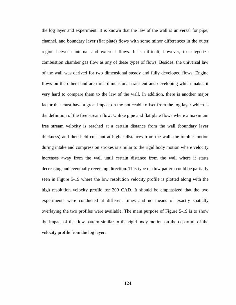
124
the log layer and experiment. It is known that the law of the wall is universal for pipe,
channel, and boundary layer (flat plate) flows with some minor differences in the outer
region between internal and external flows. It is difficult, however, to categorize
combustion chamber gas flow as any of these types of flows. Besides, the universal law
of the wall was derived for two dimensional steady and fully developed flows. Engine
flows on the other hand are three dimensional transient and developing which makes it
very hard to compare them to the law of the wall. In addition, there is another major
factor that must have a great impact on the noticeable offset from the log layer which is
the definition of the free stream flow. Unlike pipe and flat plate flows where a maximum
free stream velocity is reached at a certain distance from the wall (boundary layer
thickness) and then held constant at higher distances from the wall, the tumble motion
during intake and compression strokes is similar to the rigid body motion where velocity
increases away from the wall until certain distance from the wall where it starts
decreasing and eventually reversing direction. This type of flow pattern could be partially
seen in Figure 5-19 where the low resolution velocity profile is plotted along with the
high resolution velocity profile for 200 CAD. It should be emphasized that the two
experiments were conducted at different times and no means of exactly spatially
overlaying the two profiles were available. The main purpose of Figure 5-19 is to show
the impact of the flow pattern similar to the rigid body motion on the departure of the
velocity profile from the log layer.
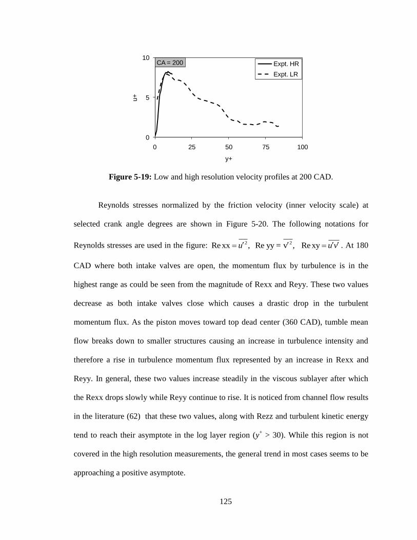
125
Figure 5-19: Low and high resolution velocity profiles at 200 CAD.
Reynolds stresses normalized by the friction velocity (inner velocity scale) at
selected crank angle degrees are shown in Figure 5-20. The following notations for
Reynolds stresses are used in the figure: 2 2Rexx , Re yy = v , Rexyu u v . At 180
CAD where both intake valves are open, the momentum flux by turbulence is in the
highest range as could be seen from the magnitude of Rexx and Reyy. These two values
decrease as both intake valves close which causes a drastic drop in the turbulent
momentum flux. As the piston moves toward top dead center (360 CAD), tumble mean
flow breaks down to smaller structures causing an increase in turbulence intensity and
therefore a rise in turbulence momentum flux represented by an increase in Rexx and
Reyy. In general, these two values increase steadily in the viscous sublayer after which
the Rexx drops slowly while Reyy continue to rise. It is noticed from channel flow results
in the literature (62) that these two values, along with Rezz and turbulent kinetic energy
tend to reach their asymptote in the log layer region (y+ > 30). While this region is not
covered in the high resolution measurements, the general trend in most cases seems to be
approaching a positive asymptote.
0
5
10
0 25 50 75 100
u+
y+
CA = 200 Expt. HR
Expt. LR

126
The peak values of the Reynolds normal stresses (Rexx and Reyy) normalized by
the friction velocity for a channel flow which was determined from Direct Numerical
Simulation (DNS) by Kim et al. (62) were found to be 7.5 and 1, respectively. The
normalized Reynolds shear stress (Rexy) had a minimum value of -0.8. Spalart (63)
obtained similar values for the Reynolds stresses normalized by friction velocity applying
DNS to a boundary layer flow over a flat plate.
Values of Reynolds stresses obtained near the cylinder head are higher than the
ones for a channel flow or a flat plate boundary layer flow. At the beginning of the
compression stroke, the peak normalized Reynolds normal stresses (Rexx and Reyy) are
75 and 35, respectively, and the minimum value of the normalized Reynolds shear stress
is -10. These values vary during the compression stroke as can been seen from Figure
5-20. They decrease in value until 230 CAD then increase gradually until 290 CAD after
which their magnitudes are amplified due to the mean flow motion (tumble) breakdown
to smaller structures as the piston moves closer to top dead center, thus enhancing
turbulence intensity. The main factor that can be attributed to the higher magnitudes of
Reynolds stresses compared to channel or flat plate flow is the cycle-to-cycle variability.
When ensemble averaging, the cycle variability is not excluded. This results in an
overestimation of the velocity fluctuations (See Chapter 3.2).
127
Figure 5-20: Normalized Reynolds stresses at selected CAD.
Turbulent kinetic energy production and dissipation (pseudo) at selected crank
angle degrees are shown in Figure 5-21.
-20
0
20
40
60
80
0 5 10 15 20 25 30
<uiu
j>/u
t^2
y+
CA = 180
Rexx
Rexy
Reyy
-20
0
20
40
60
80
0 5 10 15 20 25 30
<uiu
j>/u
t^2
y+
CA = 210
Rexx
Rexy
Reyy
-20
0
20
40
60
80
0 5 10 15 20 25 30
<uiu
j>/u
t^2
y+
CA = 230
Rexx
Rexy
Reyy
-20
0
20
40
60
80
0 5 10 15 20 25 30
<uiu
j>/u
t^2
y+
CA = 252
Rexx
Rexy
Reyy
-20
0
20
40
60
80
0 5 10 15 20 25 30
<uiu
j>/u
t^2
y+
CA = 270
Rexx
Rexy
Reyy
-20
0
20
40
60
80
0 5 10 15 20 25 30
<uiu
j>/u
t^2
y+
CA = 290
Rexx
Rexy
Reyy
-20
0
20
40
60
80
100
120
140
160
0 5 10 15 20 25 30
<uiu
j>/u
t^2
y+
CA = 310
Rexx
Rexy
Reyy
-80
0
80
160
240
320
400
480
0 5 10 15 20 25 30
<uiu
j>/u
t^2
y+
CA = 330
Rexx
Rexy
Reyy
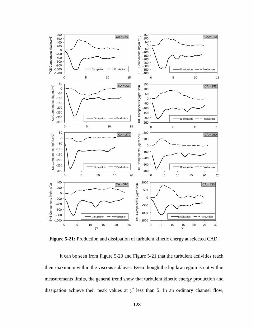
128
Figure 5-21: Production and dissipation of turbulent kinetic energy at selected CAD.
It can be seen from Figure 5-20 and Figure 5-21 that the turbulent activities reach
their maximum within the viscous sublayer. Even though the log law region is not within
measurements limits, the general trend show that turbulent kinetic energy production and
dissipation achieve their peak values at y+
less than 5. In an ordinary channel flow,
-1200
-1000
-800
-600
-400
-200
0
200
400
600
800
0 5 10 15
TK
E C
om
ponents
(kg/m
.s^3
)
y+
CA = 180
Dissipation Production
-400-350-300-250-200-150-100-50
050
100150
0 5 10 15
TK
E C
om
ponents
(kg/m
.s^3
)
y+
CA = 210
Dissipation Production
-350
-300
-250
-200
-150
-100
-50
0
50
0 5 10 15
TK
E C
om
ponents
(kg/m
.s^3
)
y+
CA = 230
Dissipation Production
-250
-200
-150
-100
-50
0
50
100
150
0 5 10 15
TK
E C
om
ponents
(kg/m
.s^3
)
y+
CA = 252
Dissipation Production
-300
-250
-200
-150
-100
-50
0
50
0 5 10 15 20
TK
E C
om
ponents
(kg/m
.s^3
)
y+
CA = 270
Dissipation Production
-400
-300
-200
-100
0
100
200
0 5 10 15 20 25
TK
E C
om
ponents
(kg/m
.s^3
)
y+
CA = 290
Dissipation Production
-1000
-800
-600
-400
-200
0
200
400
0 5 10 15 20 25
TK
E C
om
ponents
(kg
/m.s
^3)
y+
CA = 310
Dissipation Production
-1500
-1000
-500
0
500
1000
0 5 10 15 20 25 30
TK
E C
om
ponents
(kg/m
.s^3
)
y+
CA = 330
Dissipation Production
129
production peaks at y+ ~ 10 and decrease slowly until it reaches zero at y
+ ~ 400, whereas
from the current experiment results, it reaches zero at around y+ ~ 10. The main factor
that causes this significant discrepancy between the current engine results and the
ordinary flat plate or channel flow is the difference in the free stream flow pattern. While
the ordinary flat plate flow reaches a maximum at a certain boundary layer thickness
beyond which it stays constant in the free stream; in this engine, mean flow motion in the
form of tumble defines the flow pattern away from the wall which was described earlier
as an increase in velocity from zero at the wall to a maximum velocity at a certain
distance (positive gradient), then a decrease afterward until it reaches zero at the center of
the tumble motion (negative gradient) after which it increases again in the opposite
direction repeating the same pattern and creating an “S” shaped velocity profiles. Similar
pattern is found in the “plane wall jet” flow in which the bottom half of the “S” shaped
velocity profile exists and the rest the flow beyond that is quiescent. Schlichting (25)
describes the region between the wall to the point of maximum velocity (similar to the
velocity profile shown in Figure 5-19) as a two layer region consisting of a viscous wall
layer and an “internal outer layer” which starts at zero Rexy and ends at the maximum
velocity point. In this layer, the Reynolds shear stress changes sign and the turbulence
production is negative. Energy is transferred from the turbulent fluctuations to the mean
flow. This type of boundary layer behavior seems to exhibit a similar trend to the results
at hand. It also presents a good reasoning why the engine results do not follow the law of
the wall velocity distribution beyond the viscous sublayer. Figure 5-22 shows a more
detailed description of the inner-outer layer. Turbulent kinetic energy, Reynolds shear
stress, and mean velocity profile are plotted. The horizontal line in the middle of the plot
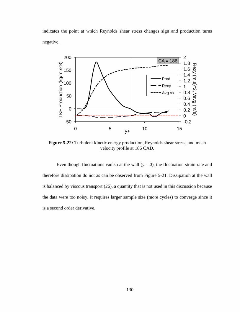
130
indicates the point at which Reynolds shear stress changes sign and production turns
negative.
Figure 5-22: Turbulent kinetic energy production, Reynolds shear stress, and mean
velocity profile at 186 CAD.
Even though fluctuations vanish at the wall (y = 0), the fluctuation strain rate and
therefore dissipation do not as can be observed from Figure 5-21. Dissipation at the wall
is balanced by viscous transport (26), a quantity that is not used in this discussion because
the data were too noisy. It requires larger sample size (more cycles) to converge since it
is a second order derivative.
-0.2
0
0.2
0.4
0.6
0.8
1
1.2
1.4
1.6
1.8
2
-50
0
50
100
150
200
0 5 10 15
Rexy (m
.s)^2
, Vavg (m
/s)
TK
E P
roduction (
kg/m
.s^3
)
y+
CA = 186
Prod
Rexy
Avg Vx

131
CHAPTER 6
CONCLUSIONS AND FUTURE WORK
The measurements presented in this thesis show that boundary layer velocity and
fluctuation intensity profiles could be resolved to within 22 μm from the cylinder head
wall of a motored internal combustion engine utilizing a combination of a μPIV and PTV
algorithm. The investigations were carried out in the pent-roof region of a production-
type engine head. A CMOS camera coupled with a long distance microscope and a dual-
cavity Nd-YLF laser were used for high-speed PIV measurements at 2.4 kHz frame rate.
Low-resolution PIV measurements were conducted to obtain flow fields that
provide a larger scale overview of the in-cylinder flow to assist the interpretation of the
high-resolution measurements. Flow deceleration started towards the end of the
compression stroke. The flow continues its gradual deceleration during the expansion
stroke until flow reversal starts around 400 CAD. It was noticed from the low resolution
raw images and velocity vector fields that the flow reversal starts near the spark plug
caused by a recirculation in the opposite direction of the mean flow near the cylinder
head wall that temporally extends towards the fuel injector to reverse the flow near the
cylinder head wall while the mean free flow preserves its original course until the instant

132
of exhaust valves open where the whole flow is totally reversed for few CAD due
to the blow down effect.
High-resolution velocity fields were measured for 98 consecutive cycles at an
engine speed of 800 RPM from 180 to 490 CAD at every other crank angle in each of
these cycles. The ensemble velocity fluctuations are of the same order of magnitude as
the mean velocities for the entire crank angle range that was studied.
The high-resolution high-speed µPIV+PTV measurements allowed identifying
and tracking of sub-millimeter sized vortical structures as they moved within the
boundary layer. In addition to the first time boundary layer results in internal combustion
engines obtained by utilizing μPIV, the highly magnified two-dimensional instantaneous
velocity vector fields provided an unprecedented substantial source of information
regarding vortex motion within the boundary layer. While the mean flow results help
understand the structure of the boundary layer velocity profile and therefore help provide
modelers with actual representation of near wall mean velocity distribution, the identified
vortices from the instantaneous velocity vector fields when sampled could offer in-depth
understanding to the momentum and energy interaction with the engine wall.
Vortex investigation near the wall and within the boundary was carried out on the
low and high resolution instantaneous flow fields. Different vortex visualization
techniques were applied on the low resolution instantaneous velocity vector fields. Sub-
millimeter vortical structures were revealed near the cylinder head. The size of extracted

133
vortex cores varied as the decomposition method is varied along with its parameters (i.e.
convection velocity in the case of Galilean decomposition and the low-pass filter domain
in the case of LES decomposition).
Swirling strength maps determined from critical-point analysis of the local
velocity gradient tensor was an effective tool that revealed most of the possible vortical
structures. It could be used in future studies to obtain vortex statistics that includes
location, size, and strength of all possible structures. Vortex visualization techniques
could be optimized in order to determine the direction of vortex rotation. The vortex
visualization and identification methods were applied to the high resolution instantaneous
velocity vector fields and structures as small as 90 μm were identified. Their rotational
direction was visualized when the high-pass filter was applied to the smallest possible
domain of two grid spacing (90 μm).
The comparison of the high resolution results with the law of the wall, along with
the investigation of turbulence kinetic energy and Reynolds stresses, led to a preliminary
conclusion that the nature of the free stream flow in internal combustion engines cannot
be approximated to that of a flat plate or channel free stream. It is believed that the engine
free stream flow, out of plane motion, density gradient in space, and temporal changes in
the flow and the fluid properties are the reasons why the law of the wall cannot be
implemented in internal combustion engines. The boundary layer and the corresponding
turbulence production seem to resemble a plane wall jet pattern.

134
Being able to resolve boundary layers in internal combustion engines is one
important step in analyzing the convective heat transfer in the combustion chamber.
Numerical simulations and the models used to close the turbulent momentum and energy
equations in engines require experimental data to support and validate the applicability of
those models in internal combustion engines. Temperature measurements near engine
walls are necessary to complement the current velocity measurements in order to provide
modelers with a complete set of validation or modification tools.
To enable the development of engine flow and heat transfer models, velocity and
fluctuations intensity profiles should be measured for the whole cycle to obtain a
complete sequence of the progression of the boundary layer. Velocity profiles should also
be measured as a function of engine speed. In conjunction with high-resolution
measurements, velocity across the cylinder should be measured to understand what drives
the evolution of the flow near the wall. Future work should also measure boundary layer
velocity profiles in other locations, such as the cylinder wall. Velocity measurements near
the cylinder wall were attempted by imaging at an angle which was not successful due to
the fact that the camera was actually projecting a three dimensional velocity motion into a
two dimensional frame. It was concluded that in order to image near cylinder wall flow
motions at an angle, a three dimensional stereo PIV must be implemented which is an
important upgrade to the current project. A two plane 3D PIV could be the next step
afterward, which would lead to a comprehensive turbulence analysis (i.e. Reynolds stress
and turbulent kinetic energy) and a better assessment for the continuity equation. Either a
simultaneous low and high resolution setups or a larger format camera is recommended
135
in order to capture more details about the outer layer since the free stream flow has
proven to have a great impact on the departure of the experimental results from the
ordinary flat plate “law of the wall”. Also, simultaneous temperature measurements
should complement boundary layer investigations in order to implement more reasonable
values of fluid properties and to ultimately provide modelers with a complete data
package of velocity, temperature, and turbulence intensity profiles along with other
turbulence statistics. Once this is accomplished, the convective heat transfer problem in
internal combustion engines can be studied comprehensively and more realistically based
on its essential fundamentals rather than by either imposing assumptions applicable to
other configurations and flow conditions (i.e. flat plate 2D flow), or deriving empirical
correlations based on a single (or multiple) point temperature/heat flux measurements.
Instead of imaging a complete engine stroke at a time, it is advisable to break it
down to smaller intervals in order to increase the sample size to obtain better statistics,
especially when analyzing higher order derivatives. This requires a very sturdy and
stable setup to insure imaging the exact same location for each set. Tracking and
sampling the coherent vortex structures in the engine boundary layers should complement
the current velocity boundary layer study to give a comprehensive foundation for
investigating heat transfer physics in IC engines, in addition to better understand
turbulence production at the engine walls.

136
BIBLIOGRAPHY
1. Borman, G. and Nishiwaki, K., “Internal Combustion Engine Heat Transfer,” Prog.
Energy Combustion Science, Vol. 13, pp. 1-46, 1987.
2. Heywood, J. B., Internal Combustion Engine Fundamentals, New York: McGraw-Hill,
1988.
3. Lumley, J. L., Engines: An Introduction, Cambridge: Cambridge University Press,
1999.
4. Dimplefield, P. A., “Study of Autoignition in a Premixed Charge, Internal Combustion
Engine using Comprehensive Chemical Kinetics; Experiments and Predictions,”
PhD Thesis, Department of Mechanical Engineering/Foster, University of
Wisconsin, Madison, 1985.
5. Kays, W., Crawford, M., and Weigand, B., Convective Heat and Mass Transfer, 4th
ed., New York: McGraw-Hill, 2006.
6. Taylor, C. F. and Toong, T. Y., “Heat Transfer in Internal Combustion Engines,”
ASME, 57-HT-17, 1957.
7. Nusselt, W., “Der Warmeubergang in der Verbrenungskraftmaschene,” Z. Verdt. Ing.,
Vol. 67, pp. 692-708, 1923.
8. Eichelberg, G., “Some New Investigations on Old Combustion Engine Problems,”
Engineering, Vol. 148, pp. 463-446, 547-560, 1939.
9. Annad, W. J., “Heat Transfer in the Cylinder of Reciprocating Internal Engines,” Proc.
Instn Mech. Engrs, 36, Vol. 177, pp. 973-990, 1963.
10. Woschni, G. A., “A Universally Applicable Equation for the Instantaneous Heat
Transfer Coefficient in the Internal Combustion Engine,” SAE, 670931, 1967.
11. Woshni, G., “Die Berechnung der Wandverluste und der Thermischen Belatung der
Bauteile von Dieselmotoren,” MTZ, 12, Vol. 20, pp. 491-499, 1970.
12. Franco, A. and Martorano, L., “Evaluations on the Heat transfer in Small two Stroke
Engines,” SAE, 98762, 1998.
137
13. Schubert, C., Wimmer, A., and Chmela, F., “Advanced Heat transfer Model for CI
Engines,” SAE, 2005-01-0695, 2005.
14. LeFeuvre, T., Myers, P. S., and Uyehara, O. A., “Experimental Instantaneous Heat
Fluxes in a Diesel Engine and Their Correlation,” SAE, 690464, 1969.
15. Chang, J., Gurlap, O., Filipi, Z., Assanis, D., Kuo, T., Najt, P., and Rask, R., “New
Heat transfer Correlation for an HCCI Engine Derived from Measurements of
Instantaneous Surface Heat Flux,” SAE, 2004-01-2996, 2004.
16. Kraiger, R. B., and Borman, G. L., “The Computation of Apparent Heat Release for
Internal Combustion Engines,” ASME, 66-WA/DGP-4, 1966.
17. Borgnakke, C., Arpaci, V. S., and Tabacsynski, R. J., “A Model for the Instantaneous
Heat Transfer and Turbulence in a Spark Ignition Engine,” SAE, 800287, 1980.
18. Payri, F., Margot, X., Gil, A., and Martin, J., “Computational Study of Heat Transfer
to the Walls of a Diesel Engine,” SAE, 2005-01-0210, 2005.
19. Fluent 6.2 User Guide, Fluent Inc., 2005.
20. Wilson, N. D., Watkins, A. J., and Dopson, C., “Asymmetric Valve Strategies and
Their Effect on Combustion,” SAE, 930821, 1993.
21. Hall, M. J., and Bracco, F. V., “Cycle-Resolved Velocity and Turbulence
Measurements Near the Cyliner of a Firing S. I. Engine,” SAE, 861530, 1986.
22. Fansler, T. D., “Turbulence Production and Relaxation in Bowel-in-Piston Engines,”
SAE, 930479, 1993.
23. Chung, T. J., Computational Fluid Dynamics, Cambridge: Cambridge University
Press, 2002.
24. Davidson, P. A., Turbulence: An Introduction for Scientists and Engineers, Oxford:
Oxford University Press, 2004.
25. Schlichting, H. and Gersten, K., Boundary Layer Theory, 8th Revised and Enlarged
Edition. Berlin: Springer, 2003.
26. Pope, S. B., Turbulent Flows, Cambridge: Cambridge University Press, 2006.
27. Adrian, R., Christensen, K., and Liu, Z., “Analysis and Interpretation of Instantaneous
Turbulent Velocity Fields,” Experiments in Fluids, Vol. 29, pp. 275-290, 2000.
28. Kline, S. J., and Rbinson, S. K., “Quasi-Coherent Structures in the Turbulent
Boundary Layer. Part I: Status Report on a Community-Wide Summary of the Data,”
Proceedings of Zaric Memorial Conference, pp. 200-217, 1989.

138
29. Chong, M., Perry, A. and Cantwell, B., “A General Classification of Three-
Dimensional Flow Fields,” Physics of Fluids A, Vol. 2, pp. 765-777, 1990.
30. Zhou, J., Adrian, R. and Balachandar, S., “Autogeneration of Near-Wall Vortical
Stryctures in Channel Flow,” Physics of Fluids, Vol. 8, pp. 288-290, 1996.
31. Zhou, J., Adrian, R., Balachandar, S., and Kendall, T., “Mechanisms for Generating
Coherent Packets of Hairpin Vortices in Channel Flow,” Journal of Fluid
Mechanics, Vol. 387, pp. 353-396, 1999.
32. Flow Master Manual: 1003005_FlowMaster_D72.pdf, Gottingen: LaVision, 2007.
33. Yeh, Y., and Cummins, H. Z., “Localized Fluid Flow Measurements with a He-Ne
Laser Spectrometer,” Applied Physics Letters, 10, Vol. 4, pp. 176-178, 1964.
34. Johnston, S. C., Robinson, C. W., Rorke, W. S., Smith, J. R., and Witze. P. O.,
“Applications of Laser Diagnostics to an Injected Engine,” SAE, 790092, 1979.
35. Barker, D. B., and Fourney, M. E., “Measuring Fluid Velocities with Speckle
Patterns,” Optics Letters, 4, Vol. 1, pp. 135-137, 1977.
36. Dudderar, T. D., and Simpkins, P. G., “Laser Speckle Photography in a Fluid
Medium,” Nature, 5632, Vol. 270, pp. 45-47, 1977.
37. Grousson, R., and Mallick, S., “Study of Flow Pattern in a Fluid by Scattered Laser
Light,” Applied Optics, 9, Vol. 16, pp. 2334-2336, 1977.
38. Meynart, R., “Instantaneous Velocity Field Measurements in Unsteady Gas Flow by
Speckle Velocimetry,” Applied Optics, 4, Vol. 22, pp. 535-540, 1983.
39. Pickering, C. J. D., and Halliwell, N. A., “Laser Speckle Photography and Particle
Image Velocimetry: Photographic Film Noise,” Applied Optics, 17, Vol. 23, pp.
2961-2969, 1984.
40. Adrian, R., “Scattering Particle Characteristics and Their Effect on Pulsed Laser
Measurements of Fluid Flow: Speckle Velocimetry vs. Particle Image Velocimetry,”
Applied Optics, 11, Vol. 23, pp. 1690-1691, 1984.
41. Raffel, M., Willert, C., Wereley, S., and Kompenhans, J., Particle Image
Velocimetry: Apractical Guide, 2nd ed., Berlin: Springer, 2007.
42. Reuss, D. L., Adrian, R. J., Landerth, C. C., French, D. T., and Fansler, T. D.,
“Instantaneous Planar Measurements of Velocity and Large-Scale Vorticity and
Strain Rate in an Engine Using Particle Image Velocimetry,” SAE, 890616, 1989.
43. Foster, D. F. and Witze, P. O., “Velocity Measurements in the Wall Boundary Layer
of a Spark-Ignited Research Engine,” SAE, 872105, 1987.
139
44. Pierce, P. H., Ghandhi, J. B., and Martin, J. K., “Near-Wall Velocity Characteristics
in Valved and Ported Motored Engines,” SAE, 920152, 1992.
45. Kline, S. J., Reynolds, W. C., Schraub, F. A., and Runstadler, P. W., “The Structure
of Turbulent Boundary Layers,” Journal of Fluid Mechanics, Vol. 30, pp. 741-773,
1967.
46. Costamagna, P., Vittori, G., and Bloneaux, P., “Coherent Structures in Oscillatory
Boundary Layers,” Journal of Fluid Mechanics, Vol. 474, pp. 1-33, doi:
10.1017/S0022112002002665, 2003.
47. Kearney, S. P., Jacobi, A. M., and Lucht, R. P., “Time_resolved Thermal Baoundary-
Layer Structure in a Pulsatile Reversing Channel Flow,” ASME Journal of Heat
Transfer, Vol. 123, pp. 655-664, doi: 10.1115/1.1372317, 2001.
48. Keane, R. D., and Adrian, R. J., “Optimization of Particle Image Velocimeters. Part I:
Double Pulsed Systems,” Measurement Science and Technology, Vol. 1, pp. 1202-
1215, 1990.
49. White, F. M., Viscous Fluid Flow, 3rd
ed., New York: McGraw-Hill, 2006.
50. Cosadia, J., Boree, J., Charnay, G., and Dumont, P., “Cyclic Variation of the Swirling
Flow in a Diesel Transparent Engine,” Experiments in Fluids, Vol. 41, pp. 115-134,
doi: 10.1007/s00348-006-0163-4, 2006.
51. Keane, R. D., and Adrian, R. J., “Optimization of Particle Image Velocimeters. Part
II: Double Pulsed Systems,” Measurement Science and Technology, Vol. 2, pp. 963-
974, 1991.
52. Megerle, M., Sick, V., and Reuss, D. L., “Measurement of Digital Particle Image
Velocimetry Precision Using Electro-Optically Created Particle-Image
Displacements,” Measurement Science and Technology, Vol. 13, pp. 997-1005,
2002.
53. Stanislas, M., Okamoto, K., Kahler, C. J., and Westerweel, J., “Main Results of the
Second International PIV Challenge,” Experiments in Fluids, Vol. 39, pp. 170-191,
doi: 10.1007/s00348-005-0951-2, 2005.
54. Specialist Committee on Uncertainty, “Uncertainty Analysis: Particle Imaging
Velocimetry,” 25th ITCC-Recommended Procedures and Guidelines, 7.5-01-03-03,
2008.
55. Luong, M., Zhang, R., Schulz, C., and Sick, V., “Toluene Laser-Induced
Fluorescence for In-Cylinder Temperature Imaging in Internal Combustion
Engines,” Applied Physics B, Vol. 91, pp. 669-675, doi: 10.1007/s00340-008-2995-
5, 2008.
140
56. Brübach, J., Zetterberg, J., Omrane, A., Li, Z. S., Alden, M., and Dreizler, A.,
“Determination of Surface Normal Temperature Gradients using Thermographic
Phosphors and Filtered Rayleigh Scattering,” Applied Physics B, Vol. 84, pp. 537-
541, doi: 10.1007/s00340-006-2243-9, 2006.
57. Fajardo, C.M., Sick, V., “Development of a High-Speed UV Particle Image
Velocimetry Technique and Application for Measurements in Internal Combustion
Engines,” Experiments in Fluids, Vol. 46, pp. 43-53, doi: 10.1007/s00348-008-0535-
z, 2009.
58. Reuss, D. L., Megerle, M., and Sick, V., “Particle-Image Velocimetry Measurement
Errors when Imaging Through a Transparent Engine Cylinder,” Measurement
Science and Technology, Vol. 13, pp. 1029-1035, pii: S0957-0233(02)31488-7,
2002.
59. Howell, S. B., Handbook of CCD Astronomy, Cambridge: Cambridge University
Press, 2000.
60. Stitou, A., and Riethmuller, M. L., “Extension of PIV to Super Resolution using
PTV,” Measurement Science and Technology, Vol. 12, pp. 1398-1403, pii: S0957-
0233(01)20955-2, 2001.
61. Fajardo, C. M., Sick, V., “Kinetic Energy and Dissipation Rate Spectra of High-and
Low-Swirl Internal Combustion Engine Flows,” SAE, 2009-01-0651, 2009.
62. Kim, J., Moin, P., and Moser, R., “Turbulence Statistics in Fully Developed Channel
Flow at Low Reynolds Number,” Journal of Fluid Mechanics, Vol. 177, pp. 133-
166, 1987.
63. Spalart, P. R., “Direct Simulation of a Turbulent Boundary Layer up to Re = 1410,”
Journal of Fluid Mechanics, Vol. 187, pp. 61-98, 1988.