High-Resolution Simulations of Lee Waves and Downslope ...

High-Resolution Simulations of Lee Waves and Downslope Winds overthe Sierra Nevada during T-REX IOP 6

PETER SHERIDAN AND SIMON VOSPER

Met Office, Exeter, United Kingdom

(Manuscript received 22 September 2011, in final form 10 February 2012)

ABSTRACT

The downslope windstorm during intensive observation period (IOP) 6 was the most severe that was

detected during the Terrain-Induced Rotor Experiment (T-REX) in Owens Valley in the Sierra Nevada of

California. Cross sections of vertical motion in the form of a composite constructed from aircraft data

spanning the depth of the troposphere are used to link the winds experienced at the surface to the changing

structure of the mountain-wave field aloft. Detailed analysis of other observations allows the role played by

a passing occluded front, associated with the rapid intensification (and subsequent cessation) of the wind-

storm, to be studied. High-resolution, nested modeling using the Met Office Unified Model (MetUM) is used

to study qualitative aspects of the flow and the influence of the front, and this modeling suggests that accurate

forecasting of the timing and position of both the front and strong mountaintop winds is crucial to capture the

wave dynamics and accompanying windstorm. Meanwhile, far ahead of the front, simulated downslope winds

are shallow and foehnlike, driven by the thermal contrast between the upstream and valley air mass. The study

also highlights the difficulties of capturing the detailed interaction of weather systems with large and complex

orography in numerical weather prediction.

1. Introduction

The Sierra Nevada range is a well-known source of

strong mountain waves, downslope windstorms, and

turbulence associated with lee-wave rotors, which rep-

resent hazards to aviation, residents, and property and

are difficult for forecasters to predict (Holmboe and

Klieforth 1957; Grubisic and Lewis 2004). Continued in-

crease in the resolution of operational numerical weather

prediction (NWP) models is expected to improve fore-

casts as the phenomena become more explicitly resolved.

Meanwhile, research into such hazards increasingly also

utilizes high-resolution NWP models (e.g., Gohm et al.

2004; Belusic et al. 2007; Agustsson and Olafsson 2007;

Jiang and Doyle 2008; Chan 2009; Reinecke and Durran

2009), many of which can be also be run in idealized

configurations (Schmidli et al. 2011; Doyle et al. 2011).

Thus, study of how high-resolution NWP models behave

over the Sierra Nevada during strong mountain-wave

events is valuable more generally.

Owens Valley, in the lee of the Sierra Nevada in

California, was the site of the recent Terrain-Induced

Rotor Experiment (T-REX), which involved a variety of

ground-based and airborne in situ and remote sensing

measurements that were focused on the period March–

April 2006 (Grubisic et al. 2008). Figure 1 shows the ge-

ography of the region (Owens Valley is identifiable by

the high, steep, quasi-two-dimensional slope of the sierra

forming its west side), some of the T-REX instrument

and sounding locations, research aircraft flight tracks, and

research automobile tracks in and around Owens Valley.

The comprehensive dataset available from T-REX affords

an opportunity for detailed comparison with model output.

Strong wave events over Owens Valley are typically

characterized by strong cross-ridge synoptic-scale winds

and stability close to mountaintop. These features favor

lee-wave trapping and low-level breaking of waves. During

the earlier, historic Sierra Wave Project (Holmboe and

Klieforth 1957), the synoptic situation conducive to the

strongest wave events was found to include a prefrontal

situation at Owens Valley. On some occasions, the gen-

erated waves may be large enough to control the winds

occurring within the valley, with extensive strong down-

slope windstorms and possible formation of rotors. These

may be referred to as dynamically forced downslope

Corresponding author address: Peter Sheridan, Met Office, FitzRoy

Rd., Exeter, EX1 3PB, United Kingdom.

E-mail: [email protected]

JULY 2012 S H E R I D A N A N D V O S P E R 1333

DOI: 10.1175/JAMC-D-11-0207.1

Unauthenticated | Downloaded 02/04/22 10:28 PM UTC

wind systems. A number of authors have discussed more-

moderate downslope winds in Owens Valley that are

forced by a thermal mechanism whereby the upstream

air mass becomes cooler than that in the valley (typi-

cally because of daytime solar warming within the

valley) and, flowing over the Sierra Nevada, induces

downslope winds by undercutting the valley atmosphere.

Jiang and Doyle (2008), in a study of diurnal variation of

downslope winds in Owens Valley, demonstrated this

effect for the case of only moderate mountaintop winds

by using observations and high-resolution modeling,

terming the flow ‘‘in-valley westerly.’’ Mayr and Armi

(2010) show further evidence from T-REX for flows of

this kind, likening them to a shallow Alpine foehn, and

a discussion by Raab and Mayr (2008) of measurements

in the valley suggests that this mechanism may also play a

part in initiation of downslope winds in dynamically forced

cases. Jiang and Doyle (2008) also present observed cases

of stronger dynamically forced waves in which the thermal

mechanism was not expected to play a part (e.g., at night).

Work by Billings and Grubisic (2008b) emphasizes the

importance of dynamical forcing by the upstream wind

and stability profile, and the wavelength of the resulting

waves, in determining the degree of penetration of west-

erly flow and suggests that the thermal mechanism assists

or controls westerly in-valley flow when dynamic forcing

is insufficient to enable complete penetration across the

valley floor (Billings and Grubisic 2008b,a).

Intensive observation period (IOP) 6 contained the

most intense downslope windstorm observed by the valley

FIG. 1. Overhead views of the T-REX instrumentation (see legend panel) and area terrain. (a) The Sierra Nevada

range and surrounding orography, showing the location of the MGAUS radiosonde release site, and an example of

the typical ‘‘racetrack’’ flight track of the BAe-146 aircraft (taken from flight B181 during 25 Mar 2006). On-road

tracks traced by the instrumented car (WOW) in the Owens Valley to the east of the Sierra Nevada are also shown.

Crosses mark the location of model profiles that have been studied. (b) Zoomed-in region showing the University of

Leeds and DRI AWS arrays concentrated around Independence in Owens Valley (DRI AWS 9 is marked). (c)

Zoomed-out view taking in the Central Valley to the west of the sierra and a broader area of the Rockies, showing

sites of weather stations from several networks, data from which form part of the TRC dataset covering Owens Valley

and the region in general. Independence is marked by a white cross in all panels.

1334 J O U R N A L O F A P P L I E D M E T E O R O L O G Y A N D C L I M A T O L O G Y VOLUME 51


instruments during T-REX, accompanied by large-

amplitude lee waves (Grubisic et al. 2008). For this study,

IOP 6 has been simulated using the Met Office Unified

Model (MetUM) in a nested, high-resolution configura-

tion. The aim is to describe the observed flow and to

compare the model results to gain insight into the model’s

ability to capture this extreme event and similar events

more generally. Times and dates will be given throughout

according to local standard time (LST), which is UTC 2

8 h. Section 2 describes briefly the T-REX observations

used and the geography of the region. Section 3 contains

a description of the model and nested-simulation setup.

The observed event is discussed in section 4, and the

modeled flow is compared in section 5. Conclusions are

summarized in section 6.

2. Observational data

During T-REX, a comprehensive set of measurements

of the flow aloft of the Sierra Nevada and in the Owens

Valley was obtained. Owens Valley is very straight, with

little variation in width along its length. It is over 100 km

long and 15 (30) km wide measured at the base (peaks) of

the bounding terrain. The sierra terrain to the west rises

roughly 3000 m above the valley floor, and occurrences

are well documented of large-amplitude mountain waves

induced by stable flow over the mountains, associated

westerly downslope windstorms sweeping across the val-

ley, or turbulent regions due to separation of such flows

within the valley. An overview and details of the instru-

mentation are given by Grubisic and Billings (2007) and

Grubisic et al. (2008). A subset of the deployed instru-

mentation is used in this study, with locations shown in

Fig. 1. At the surface, an array of automatic weather

stations (AWS) installed by the Desert Research In-

stitute (DRI) and University of Leeds measured wind,

temperature, and pressure at 10 m at locations spaced

roughly 3–5 km apart close to the town of Independence,

California, as shown in Fig. 1b. The DRI data were re-

corded as 30-s averages, and the Leeds data were recorded

as 1-min averages. During IOPs, additional measure-

ments were taken, including operation of the University

of Innsbruck Weather Station on Wheels (WOW; Mayr

et al. 2002; Raab and Mayr 2008), research-aircraft flights,

and radiosonde releases west of the Sierra Nevada and

from within the valley. WOW was an instrumented car

equipped with GPS, operating over a broader area than

the main array, measuring wind and other atmospheric

variables continuously as 30-s averages along the routes

shown in Fig. 1a. Also shown in Fig. 1a is an example of

the typical cross-valley ‘‘racetrack’’ pattern flown by the

Facility for Airborne Atmospheric Measurement (FAAM)

BAe-146 aircraft during the IOPs (6, 8, and 10) discussed

herein. Two other research aircraft [the National Science

Foundation/National Center for Atmospheric Research

(NCAR) High-Performance Instrumented Airborne Plat-

form for Environmental Research (HIAPER) and Uni-

versity of Wyoming King Air] flew similar tracks, with

cross-mountain legs roughly collocated in the horizontal

plane with the BAe-146 northern leg for the three air-

craft,1 but covering different height ranges, altogether

encompassing about 2000–13 000 m MSL (roughly 6000–

40 000 ft). The remaining markers in Fig. 1a indicate

three radiosonde release stations west of the Sierra Nevada

used during IOPs to obtain the upstream profile, in-

cluding the Mobile GPS Advanced Upper Air Sounding

System (MGAUS) platform, situated at Visalia in the

Central Valley for IOPs 6, 8, and 10. Radiosondes were

released from one of these sites every 1.5–3 h during

IOPs. In addition to the above, satellite cloud images from

the high-resolution National Oceanic and Atmospheric

Administration Geostationary Operational Environmen-

tal Satellite-10 (GOES-10) are used to find evidence of

mountain-wave activity and frontal zones. Also, data from

the so-called T-REX composite (abbreviated to TRC in

this paper) dataset, combining data from routinely oper-

ational sites in the region, run through a common quality-

control procedure and averaged to 5-min intervals, are

used to supplement the main T-REX surface data over

a broader area.

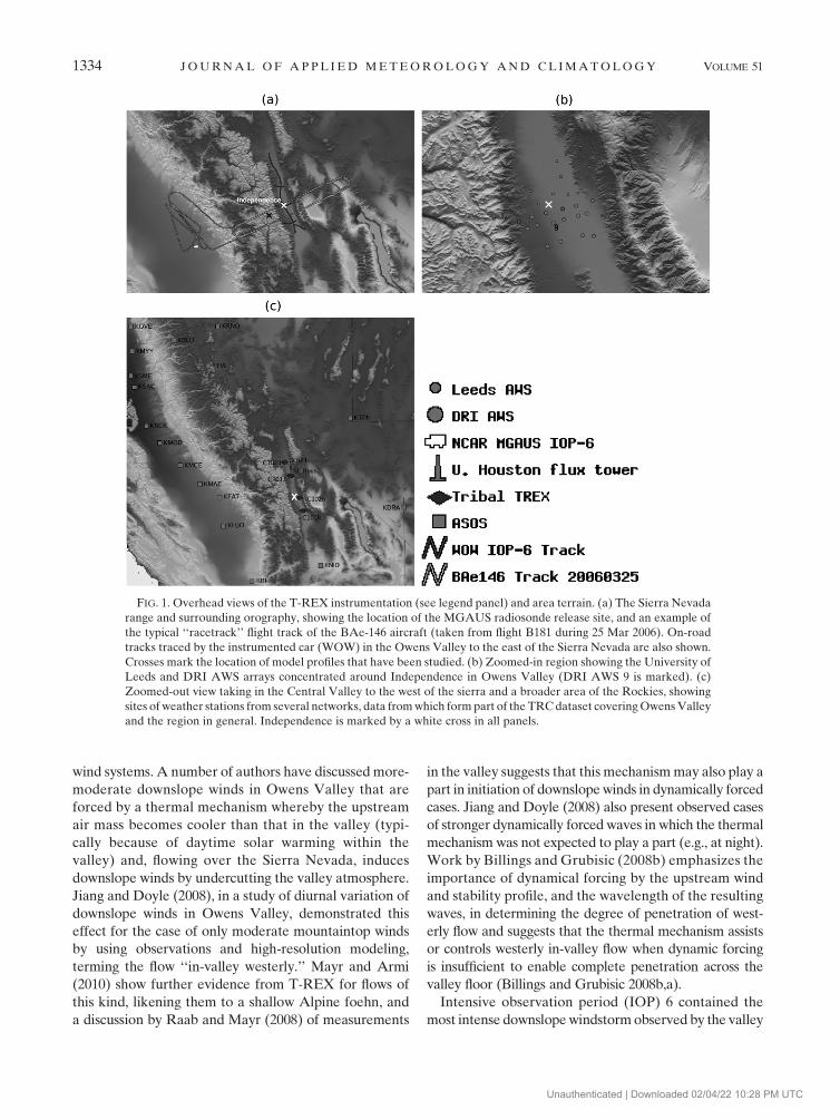
3. Model simulations

The numerical simulations were performed using

MetUM on nested grids, the outermost of which was

that of the operational global NWP configuration of the

model. The horizontal grid spacing of the global model

used was 0.56258 and 0.3758 in the zonal and meridional

directions, respectively. Forecast data from the global

model were used to initialize and drive (through lateral

boundary conditions) the flow in the higher-resolution

inner domains using a one-way nesting technique. The

inner domains had horizontal resolutions of approxi-

mately 12 km, 4 km, 1 km, and 333 m. The approximate

locations of these domains are shown in Fig. 2a.

The formulation of MetUM is described by Davies

et al. (2005). The simulations presented here were con-

ducted using version 6.1 of the model. MetUM is a finite-

difference model on a latitude–longitude grid and uses a

semi-implicit semi-Lagrangian two-time-level dynamical

core. For limited-area simulations, the latitude–longitude

grid is rotated to give a quasi-uniform grid across the

1 The HIAPER northern leg almost exactly corresponds in the

horizontal plane to the BAe-146 northern leg, and the King Air

transect is displaced roughly 4 km down valley.



domain. The 1-km- and 333-m-resolution simulations

were performed using a vertical grid that consisted of 76

levels with the model upper boundary at 39.2 km MSL.

The lowest model level is placed at 10 m above the ground,

and the grid is stretched so that the grid spacing increases

smoothly with height. At a height of 500 m, for example,

the grid spacing is approximately 110 m. At 2.5 km this

increases to around 220 m. The coarser-resolution (global,

12 km, and 4 km) domains used a similar but somewhat-

coarser-resolution vertical grid that consisted of 38 levels

and had a grid spacing of approximately 2 times that

used in the finer-resolution domains. The time-step lengths

employed in the global, 12-km, 4-km, 1-km, and 333-m

domains respectively were 15 min, 5 min, 30 s, 10 s, and 5 s.

The configuration of the model at the finest (1 km and

333 m) resolutions differed from that at the coarser

resolutions in the following ways:

1) The semi-Lagrangian advection scheme for potential

temperature involved a fully three-dimensional in-

terpolation scheme in place of the standard scheme,

which is noninterpolating in the vertical direction. Tests

have shown that this approach gives more-accurate

representation of internal gravity wave motions. This

fully interpolating scheme requires a relatively short

time step to retain numerical stability.

2) In the semi-implicit time-integration scheme, values

of 0.6 were used for the off-centering time weights.2

This value gives greater accuracy in time than do the

standard operational settings and has been shown to

be beneficial in terms of representing gravity wave

motion. Again, for numerical-stability reasons, this

change requires the use of a reduced time step.

3) The column-based parameterizations of deep and

shallow convection (Gregory and Rowntree 1990)

applied at the coarser resolutions were not imple-

mented because at these finer resolutions the con-

vective motion is largely resolved.

4) The cloud microphysical parameterizations at all

model resolutions follow those described by Wilson

and Ballard (1999), but, for resolutions of 12 km or

finer, the parameterization accounted for the effects

of advection of precipitation between grid boxes by

the three-dimensional wind field.

At all resolutions, the simulations were conducted with

a one-dimensional (vertical) boundary layer turbulence

parameterization (the model’s 8B scheme; Lock et al.

2000). For all but the finest-resolution (333 m) model do-

mains, the model orography was extracted from the

Global Land One-Kilometer Base Elevation (GLOBE)

30 arc s–resolution dataset (Hastings and Dunbar 1999),

interpolated onto the model grid. For the global, 12-km,

and 4-km configurations these data were then smoothed

using a sixth-order low-pass implicit tangent filter similar

to that described by Raymond (1988). At 1-km resolution

no smoothing was applied. For the 333-m grid, better-

resolution data were obtained from the Space Shuttle

Radar Topography Mission (SRTM) dataset (Farr et al.

2007), whose horizontal resolution is 3 arc s, or approx-

imately 90 m. These data were interpolated onto the

FIG. 2. (a) The positions and extent of the nested 12-km, 4-km, 1-km, and 333-m model domains. The 333-m

domain (not labeled) is the innermost shown. (b) The orography (m) from the 333-m-resolution model grid, on the

basis of SRTM orography.

2 Off-centering weights of 0.5 correspond to a centered-in-time

scheme and imply formal second-order accuracy; values of 1 cor-

respond to a first-order fully implicit scheme.



model grid without any smoothing, and the resulting

orography across the 333-m domain is shown in Fig. 2b.

One-way nesting was employed, with lateral boundary

conditions updated every 15 min for the innermost

(333 m) domain, every 30 min for the 1- and 4-km do-

mains, and every hour for the 12-km domain. The IOP-6

simulation was initialized with Met Office global anal-

ysis fields at 0100 LST 25 March 2006. As a basic test,

two simulations were performed of the weak–moderate-

strength waves occurring in southwesterly synoptic

flow during IOP 8 (31 March–1 April 2006) and IOP 10

(7–8 April 2006). Strong downslope windstorms did not

occur during these cases. The vertical velocities in the

333-m domain for these cases were compared with those

measured by the FAAM BAe-146 aircraft. The model

was found to perform well, given the inherent difficulty of

representatively sampling the observed and modeled

three-dimensional fields along one-dimensional tracks.

Examples are shown in Fig. 3 for southern legs of the

racetrack pattern shown in Fig. 1, in which the model

produces wave fields that are quantitatively similar to

those measured by the aircraft.

Idealized MetUM simulations at 1-km resolution

were also carried out as sensitivity tests to various as-

pects of the upstream profile of wind and temperature

(discussed later). These used dynamical and physics set-

tings and start times that are identical to those of the

nested simulations but with simulation of only the 1-km-

resolution domain. Also, rather than using data from the

4-km-resolution simulation to initialize the 1-km domain

and update its lateral boundaries, the initial state and

lateral boundaries were set using a single horizontally ho-

mogeneous profile. Several simulations were performed,

each using a different profile, to represent different syn-

optic conditions as discussed within section 5.

4. Observed event during IOP 6

A strong wave/rotor event was documented during

IOP 6, involving a severe downslope windstorm and

separation of the flow from the valley floor, resulting in

a turbulent rotor region in the flow (Grubisic et al. 2008).

In this section, we present a summary of the observa-

tional evidence from IOP 6.

a. Synoptic evolution

Figures 4a–d show the synoptic development that oc-

curred during IOP 6 in the form of mean sea level

pressure, wind vectors at 5 km over the western United

States, and low-level temperatures from the global MetUM

forecast. Although some details may differ, the forecast

may reasonably be expected to reproduce the actual

broad synoptic situation well on the scale shown. Figure

4a indicates a depression moving inland at 0400 LST

25 March 2006, with an approaching region of strong

west-southwesterly winds, which eventually passes over

Owens Valley, and an associated front off the coast of

California (discernible as a sharp gradient in the shaded

temperature field to the south of the low center). Note

that Steenburgh et al. (2009) performed a study that

FIG. 3. Vertical velocities measured by the BAe-146 aircraft (solid lines) along the southern legs of the racetrack

pattern above the Sierra Nevada during (a)–(c) IOP 8 and (d)–(f) IOP 10. Also shown are the MetUM predictions of

vertical velocity (dashed lines) on the 1-km grid at approximately the same times as the times of the measurements.

The heights of the legs are shown in thousands of feet.



focused on the front associated with this system, which is

occluded as it encounters the terrain. Because of the

terrain-following nature of the model level whose tem-

perature is depicted, high terrain appears colder in the

plot and the rough location of the Sierra Nevada can be

discerned from a finger of cold temperatures in the

western United States. At 1000 LST (Fig. 4b), the wind

has strengthened over the sierra, and the front has

made landfall. By 1600 LST (Fig. 4c), around the time of

the windstorm, the front is by now interacting with the

mountain topography of the region and is no longer

easily discernible, the low center has become a trough

over the Pacific coast to the northwest, and the winds

over the sierra have begun to turn more westerly. Later by

2200 LST (Fig. 4d) the system has progressed inland,

replaced by a ridge approaching from the west.

The synoptic flow is further illustrated by the wind and

potential temperature profiles in Fig. 5. The thick solid

black line represents a radiosonde ascent from upstream

of the Sierra Nevada. This profile indicates a layer of

enhanced stability close to the ridgetop, where strong

west-southwest winds also occur, and strong positive ver-

tical wind shear in the troposphere. A stable layer and

northerly near-surface jet below 1 km MSL reflect the

passage of the front at the launch location that occurred

about an hour before the time of the sounding.

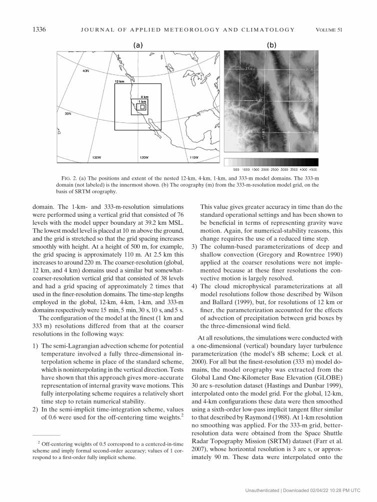
b. Gravity waves

Figures 6a–d show four GOES-10 visible satellite images

over the western United States between 1030 and 1730 LST

25 March 2006. Well-developed lee waves are evident

downstream of the coastal mountains and Sierra Nevada.

The three research aircraft detected gravity wave mo-

tion in the variation of vertical velocity. A method fre-

quently used for studying gravity wave motion is to plot

vertical velocities for individual flight legs during a wave

FIG. 4. The MetUM forecast synoptic evolution during IOP 6. Quantities shown are global-resolution model fields of

pressure at mean sea level (thick black contours; interval is 5 hPa), wind vectors at 5 km above sea level, and temperature

(K; shading and white contours) on model level 9, which is approximately 1600 m MSL, at (a) 0400, (b) 1000, (c) 1600,

and (d) 2200 LST 25 Mar 2006. Coastline (thin black line) and location of Independence (cross) are also shown.



event. Here, measurements from legs at different heights

have instead been interpolated to give a single composite

vertical valley cross section for a given period. Inter-

polation onto a regular grid was performed by the

‘‘GETMAT’’ matrix function of the ‘‘DISLIN’’ graphics

library. This function performs a weighted average of

the observations on the basis of horizontal and vertical

ranges of influence and a weighting factor. A small area

of influence and high weighting factor emphasize local

detail. The grid was chosen to reflect the relative density

of data in the vertical (30 grid points) and horizontal

(1000 grid points) directions, with area of influence be-

ing two points in the vertical direction and four points in

the horizontal plane, using the default weighting factor.

Artifacts exist beyond the outer (i.e., top and bottom)

flight legs because of extrapolation. Boundary condi-

tions, for instance of zero vertical velocity, were not used

because they would artificially reduce contour values

near the surface and be unrealistic at the upper bound-

ary. This unique synthesis, possible only because of the

simultaneous deployment of the three aircraft, provides

a convenient visualization of the wave field and facilitates

easy comparison with model cross sections. Northern

flight legs, which were collocated in the horizontal plane

for all three aircraft, have been used to create the

composites. Figures 7a and 7b show composites that are

based on data from a part of the IOP between 0820

and 1115 LST and from a later part between 1300 and

1630 LST 25 March, respectively. Note that these 3–3.5-h

intervals are sufficiently long for the waves to have evolved

somewhat between the initial and final legs used for the

interpolation and that the composites cannot be con-

sidered to be true instantaneous snapshots of the flow.

In Fig. 7a, the uppermost (HIAPER) measurement legs

took place between 0945 and 1115 LST, the BAe-146

legs and the upper King Air legs above mountain crest

took place between 0820 and 1115 LST, and the lower

King Air legs took place between 1000 and 1100 LST.

In Fig. 7b, the uppermost (HIAPER) measurement legs

took place between 1300 and 1430 LST, the BAe-146

legs above mountain crest took place between 1440

and 1630 LST, and the shorter King Air legs took place

FIG. 5. Comparison of profiles recorded by radiosondes and aircraft with profiles through the 1-km-resolution MetUM domain at similar

locations: MetUM profiles at 1500 LST 25 Mar (thin solid lines) and 1700 LST (thin dashed lines), the profile detected by the radiosonde

released from the MGAUS station at 1458 LST 25 Mar (thick solid lines), and the profile detected by the BAe-146 at 1731 LST 25 Mar

(thick dashed lines). The aircraft track corresponding to the 1731 LST profile lies within the short flight legs, oriented roughly along the

San Joaquin Valley, in the westernmost part of the flight track shown in Fig. 1a.



between 1520 and 1600 LST, the legs being flown in

descending order for all three aircraft. Despite time

differences, adjacent legs flown at different times by dif-

ferent aircraft seem to mesh reasonably well, except

perhaps the King Air and BAe-146 legs in Fig. 7b, and

this result may reflect the rapid evolution of this lower

portion of the wave field at this time.

The aircraft composites provide a revealing depiction

of the wave field structure, in which vertical motion is

weak upstream of the mountains, with large up- and

downdrafts downstream associated with the wave mo-

tion. The vertical orientation of up- and downdraft re-

gions in both Figs. 7a and 7b would normally suggest that

the wave field in the mid–low troposphere is (partially)

trapped. In the earlier of the two aircraft composites (Fig.

7a), the waves are characterized by a strong downdraft

into the Owens Valley followed by an updraft of similar

strength, also over the valley, and then alternating up-

and downdrafts of decaying strength farther downstream.

In the later period (Fig. 7b) the waves are much stronger

and the primary downdraft is shifted significantly down-

stream, beyond Independence, while the wavelength of

the rest of the wave train is slightly longer so that the first

updraft spreads beyond the peak of the Inyo Mountains

on the east side of the valley. The shift of the primary

downdraft also appears to be visible in the wave clouds in

Fig. 6 using the Independence airfield as a reference, with

notable development in Fig. 6c at 1530 LST: the initially

straight edge of the ‘‘cap’’ cloud above the crest becomes

disturbed, with parts extending farther out from the crest.

This change becomes more pronounced by 1600 LST (not

shown). The King Air tracks in the lower troposphere

measured the largest (and most turbulent) motions.

The distribution of wave motion in the vertical di-

rection also differs between the two panels of Fig. 7. The

depth of atmosphere sampled appears to be split into

two regions from this point of view: one close to the tro-

popause and the other below this level and occupying the

remaining depth of the troposphere. Where waves are

strongest in one of these regions, they appear weaker in

the other region, above a given point in the horizontal

plane. This would seem to reflect the degree to which

waves are ‘‘ducted’’ within different layers. In Fig. 7a, the

strong waves close to the tropopause appear like trapped

waves, although they were measured over three HIAPER

legs spaced over a somewhat narrow vertical range of

around 1.4 km, making it difficult to be conclusive. There

is a phase disconnect between these waves and those at

FIG. 6. Images from the visible channel of GOES-10 at (a) 1030, (b) 1200, (c) 1530, and (d) 1730 LST 25 Mar 2006.

Lines of latitude and longitude, coastlines, and state boundaries are marked in white. Black and white thick crosses

denote the positions of the Fresno (west of the sierra) and Independence airfields, respectively.



the lower levels. Smith et al. (2008) and Woods and Smith

(2010) undertook detailed study of the HIAPER data

during T-REX IOPs using Fourier and wavelet analysis

methods, building a detailed picture of wave propagation.

They discovered trapped waves of relatively short wave-

length at the tropopause during IOP 13 (thought to be

secondary waves generated locally by a wave-steepening

mechanism) coexisting with longer-wavelength upward-

and downward-propagating waves within the troposphere,

but similar evidence was not presented for IOP 6. Instead,

Woods and Smith (2010) discuss downward-propagating

waves coexisting with the primary upward-propagating

wave at a height of 13 km during IOP 6. Smith et al. (2008)

and Woods and Smith (2010) do not draw conclusions

concerning the wave behavior lower in the troposphere

during IOP 6.

Reinecke and Durran (2009) used an ensemble of high-

resolution nested simulations to model this flow, finding

strong sensitivity to variation of synoptic conditions. In

ensemble members containing weaker waves, the pri-

mary downdraft remained confined over the upper part

of the sierra downslope (similar to Fig. 7a), whereas in

the strongest members the wave downdraft was found

to extend farther east (in common with Fig. 7b). In the

latter cases, this structure was associated with wave

breaking.

c. Flow within the valley

A time series of the wind speed and direction at DRI

AWS 9 is shown in Fig. 8 (solid lines). Until 1530 LST

25 March, flow was variable and episodical, on the whole

being either up valley (roughly southerly) or more west-

erly or southwesterly (cross valley), seldom increasing

above 10 m s21 in strength. The wind strengthened and

steadied after this time. A particularly intense westerly

downslope flow subsequently commenced after 1735 LST

FIG. 7. Vertical velocities (color contours; m s21) measured by the King Air, BAe-146, and

HIAPER aircraft during IOP 6. Data shown are from the northern legs between (a) 0820 and

1115 LST and (b) 1300 and 1630 LST 25 Mar and have been interpolated between the flight legs

to provide a composite image (see text). The horizontal lines depict the aircraft trajectories

projected onto the vertical plane. Also shown is the orography beneath the path of HIAPER.



peaking at 24 m s21 and ending abruptly at 1851 LST

in a transition to a northerly down-valley flow. This

intense windstorm was observed throughout the In-

dependence AWS array, including the easternmost sta-

tions at the foot of the Inyo Mountains, peaking at close

to 30 m s21 at some sites. A snapshot of wind vectors

from the most intense part of the windstorm in shown in

Fig. 9a. The windstorm was observed (on the basis of the

whole AWS array) to both grow and diminish starting in

the east of the valley, suggesting that a thermally driven

flow from passes within the sierra barrier was not its

primary driver. The windstorm is presumably connected

with the change in wave structure detected by the aircraft

just beforehand (Fig. 7b), suggesting a primarily dy-

namically forced downslope-flow case. Note that, in the

ensemble of high-resolution nested simulations of this

flow of Reinecke and Durran (2009), strong downslope

winds were directly linked with a breaking-wave structure

aloft.

Of interest is that examination of TRC stations within

the Owens Valley (see Fig. 1) and the WOW instrumented

car data did not reveal such exceptionally intense, and

consistently westerly, flow elsewhere in the valley (not

shown). Only C1028, located within the Independence

array, detected winds of exceptional strength, peaking at

29 m s21 at 1830 LST, while winds at the other TRC

stations within the valley in Fig. 1 detected nothing over

15 m s21. Jiang et al. (2011) also report winds peaking

over 25 m s21 west of Owens Lake around this time. This

suggests that the main windstorm may have been rela-

tively localized to these areas.

d. Attribution

Analysis of synoptic details and of the timing of the

observed wave evolution and windstorm affords some

insight into the possible precursors of such a dramatic

event. As already mentioned, strong mountaintop wind

and stability are expected to be important factors in the

FIG. 8. Comparisons of time series of the observed (solid) and

modeled (dashed) wind speed and direction for the period 0700–

2200 LST 25 Mar for DRI AWS 9 in Owens Valley. The model

data are 1-min instantaneous predictions at 10 m and are taken

from the 333-m grid, the AWS data are 30-s averages of measure-

ments also at 10 m.

FIG. 9. (a) The 10-m wind field measured by the DRI and University of Leeds AWS array in the Owens Valley at

1828 LST 25 Mar. The colored dots indicate the wind speed (m s21). Data were recorded as 30-s and 1-min averages

by the DRI and University of Leeds instruments, respectively. (b) The model instantaneous 10-m wind field on the 333-m

grid at 1716 LST 25 Mar, zoomed over the same area as shown in (a). The color contours indicate wind speed (m s21).



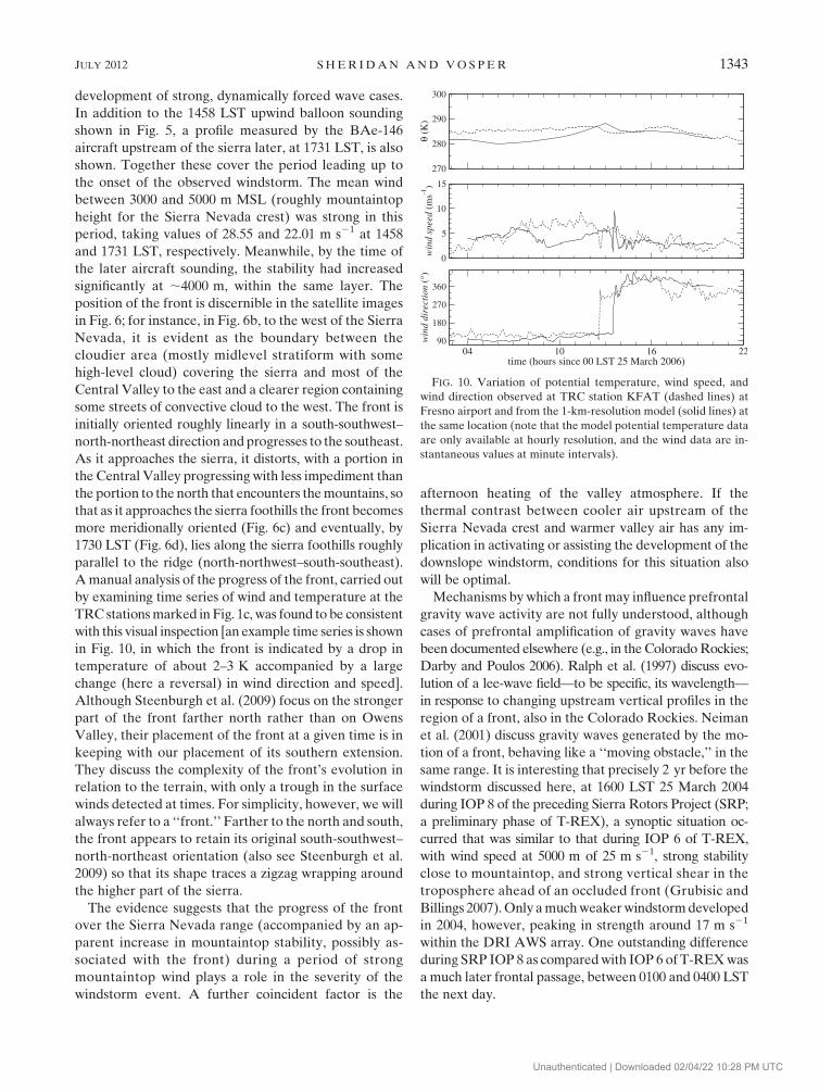
development of strong, dynamically forced wave cases.

In addition to the 1458 LST upwind balloon sounding

shown in Fig. 5, a profile measured by the BAe-146

aircraft upstream of the sierra later, at 1731 LST, is also

shown. Together these cover the period leading up to

the onset of the observed windstorm. The mean wind

between 3000 and 5000 m MSL (roughly mountaintop

height for the Sierra Nevada crest) was strong in this

period, taking values of 28.55 and 22.01 m s21 at 1458

and 1731 LST, respectively. Meanwhile, by the time of

the later aircraft sounding, the stability had increased

significantly at ;4000 m, within the same layer. The

position of the front is discernible in the satellite images

in Fig. 6; for instance, in Fig. 6b, to the west of the Sierra

Nevada, it is evident as the boundary between the

cloudier area (mostly midlevel stratiform with some

high-level cloud) covering the sierra and most of the

Central Valley to the east and a clearer region containing

some streets of convective cloud to the west. The front is

initially oriented roughly linearly in a south-southwest–

north-northeast direction and progresses to the southeast.

As it approaches the sierra, it distorts, with a portion in

the Central Valley progressing with less impediment than

the portion to the north that encounters the mountains, so

that as it approaches the sierra foothills the front becomes

more meridionally oriented (Fig. 6c) and eventually, by

1730 LST (Fig. 6d), lies along the sierra foothills roughly

parallel to the ridge (north-northwest–south-southeast).

A manual analysis of the progress of the front, carried out

by examining time series of wind and temperature at the

TRC stations marked in Fig. 1c, was found to be consistent

with this visual inspection [an example time series is shown

in Fig. 10, in which the front is indicated by a drop in

temperature of about 2–3 K accompanied by a large

change (here a reversal) in wind direction and speed].

Although Steenburgh et al. (2009) focus on the stronger

part of the front farther north rather than on Owens

Valley, their placement of the front at a given time is in

keeping with our placement of its southern extension.

They discuss the complexity of the front’s evolution in

relation to the terrain, with only a trough in the surface

winds detected at times. For simplicity, however, we will

always refer to a ‘‘front.’’ Farther to the north and south,

the front appears to retain its original south-southwest–

north-northeast orientation (also see Steenburgh et al.

2009) so that its shape traces a zigzag wrapping around

the higher part of the sierra.

The evidence suggests that the progress of the front

over the Sierra Nevada range (accompanied by an ap-

parent increase in mountaintop stability, possibly as-

sociated with the front) during a period of strong

mountaintop wind plays a role in the severity of the

windstorm event. A further coincident factor is the

afternoon heating of the valley atmosphere. If the

thermal contrast between cooler air upstream of the

Sierra Nevada crest and warmer valley air has any im-

plication in activating or assisting the development of the

downslope windstorm, conditions for this situation also

will be optimal.

Mechanisms by which a front may influence prefrontal

gravity wave activity are not fully understood, although

cases of prefrontal amplification of gravity waves have

been documented elsewhere (e.g., in the Colorado Rockies;

Darby and Poulos 2006). Ralph et al. (1997) discuss evo-

lution of a lee-wave field—to be specific, its wavelength—

in response to changing upstream vertical profiles in the

region of a front, also in the Colorado Rockies. Neiman

et al. (2001) discuss gravity waves generated by the mo-

tion of a front, behaving like a ‘‘moving obstacle,’’ in the

same range. It is interesting that precisely 2 yr before the

windstorm discussed here, at 1600 LST 25 March 2004

during IOP 8 of the preceding Sierra Rotors Project (SRP;

a preliminary phase of T-REX), a synoptic situation oc-

curred that was similar to that during IOP 6 of T-REX,

with wind speed at 5000 m of 25 m s21, strong stability

close to mountaintop, and strong vertical shear in the

troposphere ahead of an occluded front (Grubisic and

Billings 2007). Only a much weaker windstorm developed

in 2004, however, peaking in strength around 17 m s21

within the DRI AWS array. One outstanding difference

during SRP IOP 8 as compared with IOP 6 of T-REX was

a much later frontal passage, between 0100 and 0400 LST

the next day.

FIG. 10. Variation of potential temperature, wind speed, and

wind direction observed at TRC station KFAT (dashed lines) at

Fresno airport and from the 1-km-resolution model (solid lines) at

the same location (note that the model potential temperature data

are only available at hourly resolution, and the wind data are in-

stantaneous values at minute intervals).



5. Modeling of IOP 6

a. Reproducing synoptic factors

Simulating the conjunction of the factors implicated in

generating the windstorm proves difficult. The peak in

wind activity in the model is somewhat weaker than is

observed and occurs too early. The mean wind between

3000 and 5000 m decreases in strength approaching the

time of the observed windstorm, taking values at 1500,

1600, 1700, 1800, and 1900 LST of 23.6, 22.6, 16.4, 13.4,

and 13.0 m s21, respectively (also see Fig. 5). The profile

of potential temperature at 1700 LST from the model

shown in Fig. 5 also suggests underpredicted stabiliza-

tion of the profile near the mountaintop.

By comparing time series at the TRC station locations

in the 4-km model domain (and the 1-km domain where

possible) with those observed, the front was found to

approach the sierra and move down the Central Valley

to the west generally 1–2 h late in the model (see Fig. 10;

a result that is also supported by sounding comparisons

such as that in Fig. 5 for the MGAUS location). Over the

mountain area, by the time it reaches the main part of

Owens Valley the modeled front ‘‘catches up’’ with the

observations. The valley and mountain analyses taken

together indicate that the modeled front’s shape must

experience less of the distortion exhibited by the actual

front, mostly retaining its original south-southwest–

north-northeast, cross-ridge orientation. This becomes

evident in high-frequency animations of snapshots of the

wind and potential temperature fields from the model,

most discernible as the progress of a line of coherent dis-

turbance in the wind vectors. Because only still images

may be included here, the position of the front is indicated

by arrows in Figs. 12a and 12b (described below). The

front is just touching the northern tip of Owens Valley

and is still aligned roughly north-northeast–south-

southwest. The front appears to manifest itself in Owens

Valley by the onset of strong down-valley flow.

In summary, the simulation does not capture the pre-

cise conjunction of synoptic precursors of the windstorm

at Independence, with the decay in synoptic wind oc-

curring too early and the front arriving late (and in a dif-

ferent alignment). In light of this finding, two useful

investigations may be performed: 1) an investigation into

the performance of the model at Independence, taking

advantage of the high density of observations, to see to

what extent the high-resolution model gives a represen-

tative picture despite synoptic inaccuracies and 2) an in-

vestigation to examine the 333-m domain at the location

where synoptic precursors do coincide. Both of these have

implications for the interpretation of future operational

forecasting systems as resolution increases to levels that

are comparable to today’s research models.

b. Simulated waves near Independence

Figures 11a and 11b show vertical cross sections of the

vertical velocity field from the 1-km-resolution domain

of the nested MetUM simulations. As with the measured

waves, the simulated waves are characterized by a strong

downdraft and updraft over the Owens Valley, reaching

their strongest by 1700 LST 25 March (Fig. 11b). The

deep eastward spread of the primary downdraft beyond

Independence detected by the aircraft around the time

of the windstorm, however, is absent, with the modeled

wave structure in Fig. 11b instead continuing to resemble

that measured earlier on (Fig. 7a). The waves also take

later to develop (cf. the times of Figs. 11a and 7a). The

waves subsequently decay, changing phase and short-

ening in wavelength (not shown). Examination of the

vertical velocity at 5-km altitude (not shown) confirms

similar behavior along the length of the ridge.

If one leaves aside timing differences, the similarity in

structure of the waves and distribution of wave ampli-

tude in Fig. 11b to the aircraft-based composite in Fig. 7a

is strong in, for example, the waves on the tropopause,

the weakness of the second downdraft over Owens Valley

at lower levels, and the simulation of the downdraft max-

imum immediately downstream of the Inyo Mountains.

In Fig. 11b, phase lines do not appear to be vertical,

slanting both upward and downward in different parts

of the section—a result that suggests consistency with

the description of superposed upward- and downward-

propagating waves that was given by Woods and Smith

(2010) for this case.

c. Simulated winds near Independence

Model winds at DRI AWS 9 are overlaid with the

measured wind in Fig. 8. Before the westerly event, the

flow is in a roughly up-valley regime. The strengthening

of winds in the valley after 1500 LST is apparently cap-

tured by the model (although the simulated wind direction

is more steadily westerly). Later, periods of stronger

westerly or southwesterly flow, centered around 1700

and 1800 LST, occur in the model but generally stay

below 16 m s21; these periods are part of a broader,

pulsing outflow from Kearsarge Pass just west of In-

dependence, which is most well developed just after

1700 LST. Numerous such flows in the valley can be seen

developing at earlier times in Figs. 12a and 12b, which

depict snapshots of the near-surface flow at 1507 and

1600 LST, respectively. If one allows time for advection

from the MGAUS sounding location, the above flows

coincide roughly with the period of peak mountaintop

winds in the model. As the modeled synoptic winds

subsequently drop, the windstorm observed at DRI AWS

9 between 1700 and 1900 LST is absent in the model, the



wind there instead diminishing and becoming variable

before the transition to northerly down-valley flow around

1900 LST. The strong westerly flow at 10 m in the model

near Independence at 1716 LST is shown in Fig. 9b for

comparison with the observed windstorm. Although

mistiming and underestimating the observed windstorm

in strength and seemingly lacking the link to the wave

motion aloft, the model appears to be representative in

a more qualitative sense, with areas of slacker or re-

versed flow in both the model and the AWS winds at

the edge of the flow and where it terminates in the east

of the valley. From the perspective of future forecasting

systems, it is encouraging that some useful guidance as

to the occurrence of strong westerly flow within the valley

at Independence (and strong wave motion aloft), at close

to the right time, would be gained from the model. A

similarly high-resolution nested simulation of IOP 6 over

Owens Lake by Jiang et al. (2011) also significantly un-

derpredicts downslope wind strength. They find, however,

that the predicted winds are essentially sufficient for the

practical purpose of predicting aerosol lofting.

To investigate the mechanism for the downslope flow

in the model, profiles of the modeled potential temper-

ature at Independence and above the ridge crest directly

upwind (locations shown in Fig. 1) were plotted for

different stages of the flow, as shown in Fig. 13. Before

the period of sustained westerly and southwesterly flow

in the model, Fig. 13a shows little difference between the

two profiles. The onset of the flow occurs as the valley

profile warms and becomes less stable in the afternoon,

as shown in Fig. 13b (the crest profile also cools during

this time). During the period of most intense westerly

flow in the model, the base of the crest profile is now

lower in potential temperature than is almost the entire

depth of the valley atmosphere (Fig. 13c). The westerly

flow is shallow and is accompanied by an area of reversed

flow in the upper part of the valley atmosphere (not

shown). It is clear that when the potential temperature

FIG. 11. Vertical slices showing vertical velocity (color contours; m s21) and potential temperature (line contours;

interval is 2 K) along the northern leg of the aircraft tracks (see Fig. 1) at (a) 1300 and (b) 1700 LST 25 Mar in the

1-km nested simulation domain. Also shown are similar cross sections from idealized 1-km-resolution simulations

driven by (c) using a profile taken from upstream of the sierra ridge within the nested simulation and (d) using the

same profile but with winds from the 1458 LST 25 March MGAUS sounding used below 7 km (shown at 1400 LST);

(e) as in (d) but with temperatures from the BAe-146 profile run included (shown at 1400 LST); (f) as in (d) but with

the radiation parameterization inactive (shown at 1800 LST). (See main text for further details.)



at the crest becomes lower than that at some depth

within the valley atmosphere the conditions favor

penetration of the west-southwesterly flow aloft far-

ther into the valley, from buoyancy considerations.

As the flow subsequently dies, the temperature contrast

also diminishes (Fig. 13d), now because of cooling and

stabilization of the valley atmosphere in the evening.

The above behavior mirrors the diurnal cycle discussed

by Jiang and Doyle (2008). To make the connection be-

tween the ridge–valley air potential temperatures and

development of the ‘‘in-valley westerly’’ flow more ob-

vious, we define the depth of penetration of westerly

flow into the valley by two measures: hle, the height of

the ground surface at the leading (eastern) edge of the

modeled windstorm, and xpen, the eastward extent of the

windstorm at its leading edge with respect to the base

of Kearsarge Pass, just west of Independence. Both of

these measures are determined within the quadrilateral

depicted in Fig. 9b, with xpen defined by the farthest

point east where the zonal wind component exceeds

8 m s21. These are plotted as time series in Fig. 14a in

addition to heq, the height below which the valley air

(dotted lines in Fig. 13) is lower in potential temperature

than that at the base of the ridgetop profile (dashed lines

in Fig. 13). The decrease of heq as the valley atmosphere

warms (and the ridgetop profile cools) is coupled closely

with xpen. Meanwhile, hle decreases faster than might

be expected from the decrease of heq. These are un-

likely to follow each other exactly, however, since the

momentum of the downslope wind will cause overshoot

at the point of buoyant equilibrium, and mixing between

the downslope flow and the valley atmosphere as a result

of strong shear between them may also assist penetra-

tion by reducing the temperature gradient that inhibits

descent.

The profile measured by a radiosonde launched from

Independence at 1456 LST 25 March has been added to

Fig. 13b. Assuming that the model represents the ridgetop

profile sufficiently well for comparison (the upstream

MGAUS profile is fairly well replicated at this time; see

Fig. 5), it seems that at 1500 LST the profiles favor pene-

tration of winds into the valley atmosphere as in the model,

and this may explain why the model reproduces the initial

strengthening of wind shown in Fig. 8 just after this time.

This hints at the possibility of the thermal mechanism as-

sisting within the development of the observed windstorm.

In light of the differences between the modeled and

observed waves and downslope winds, and their attri-

bution to synoptic factors, some idealized tests were per-

formed (as described in section 3) to demonstrate the

sensitivity of the flow to the inaccuracies in the conditions

upwind of Independence that are fed through from the

FIG. 12. The model 10-m wind field across the Owens Valley on a zoomed area of the 333-m grid at (a) 1507 and (b)

1600 LST 25 Mar, during IOP 6. The quantities shown are wind speed (color contours; m s21), wind direction

(arrowheads), and terrain-height contours (interval 500 m). Also shown is the location of cross sections shown in

Fig. 15 (thick white line) and the location of Independence (large white cross).



driving simulation. Simulations were run for 36 h to allow

the wave field to develop, with the representative time

taken as when the strongest waves occur over Indepen-

dence. A control simulation was performed, driven using

the profile above the grid point closest to the MGAUS

release site from the 1-km domain of the nested simulation

at 1500 LST 25 March, shown in Fig. 11c. This produced

a primary downdraft similar to that in the nested simulation

shown in Fig. 11a, although with a broader subsequent

updraft over Owens Valley, spreading as far as the Inyo

crest. Because of this last difference we will focus on the

sensitivity of the primary downdraft (which in any case is

the principal feature affecting the flow in the valley) and

more generally on the wavelength and amplitude of the

waves. The results of three tests are shown in Figs. 11d–f:

1) replacing the winds in the control simulation below

roughly 7 km with those from the 1458 LST MGAUS

profile and using the MGAUS moisture profile (Fig. 11d),

2) additionally incorporating the temperature pro-

file measured by the BAe-146 aircraft at 1730 LST

(Fig. 11e), and 3) repeating test 1 but with the radiation

parameterization disabled (Fig. 11f). This allows one to

assess the impact of 1) the underprediction of synoptic-

scale winds (and wind shear) at mountaintop level by the

model, 2) the underprediction of increased stability at

mountaintop level in the model (stability that we specu-

late may be related to the approaching front), and 3) af-

ternoon heating and mixing of the valley atmosphere at

the time of the windstorm. For the two alterations of the

driving profile it was possible to match the observational

data seamlessly into the model profile by appropriate

choice of the precise heights within which to insert the

data (see Fig. 5).

Figure 11d indicates that inserting the observed winds

below 7 km results in stronger waves and a more pene-

trative downdraft over the valley; the wavelength of the

FIG. 13. Profiles of modeled potential temperature directly above Independence (dotted lines) and above the ridge

crest at the location shown in Fig. 1a directly upwind of Independence (dashed lines) at (a) 1200, (b) 1500, (c) 1700,

and (d) 1830 LST 25 Mar 2006. Profiles measured by radiosondes released from the MGAUS station (solid line) at

1458 LST and Independence airport (dot–dashed line) at 1456 LST have also been included in (b).



waves is also slightly longer than in the control simula-

tion, with the subsequent updraft spreading beyond the

Inyo ridgetop. In Fig. 11e, adding the stronger stable layer

from the BAe-146 profile run has no significant further

impact on the amplitude of the waves over Owens Valley,

but again penetration of the downdraft into the valley is

greater, and this time with the strongest portion of the

downdraft spreading deeper downslope. Figure 11f shows

the importance of daytime heating of the valley atmo-

sphere: without it, a stable boundary layer is present, lim-

iting the downdraft to a relatively shallow penetration into

the valley, resulting in much weaker waves, and shel-

tering of the valley bottom from strong winds. While the

precise effect of the observed front, and perhaps cyclone

structure too, is unlikely to be replicated by tests 1 and 2

since they employ horizontally homogeneous condi-

tions, the above idealized tests demonstrate sensitivity

to changes in upstream conditions associated with these

synoptic factors, which is consistent with the differences

seen between the observations and the nested simulation.

Furthermore, the importance of the valley temperature

structure with regard to the response of the wave field to

the underlying topography is underlined by test 3. Sim-

ulation tests 1–3 taken together make the point that a

combination of factors may be responsible for windstorms

such as that during IOP 6, so that timing within the evo-

lution of local and upstream conditions fed down from the

driving simulation is crucial.

It is not clear to what extent linear or nonlinear pro-

cesses are responsible for the observed wave evolution

and downslope windstorm. A simple exercise using a

one-dimensional Taylor–Goldstein solver was consid-

ered, but it takes no account of the details of the

underlying topography, whose double-ridge shape has

been shown to be of importance to wave structure at

this location (Grubisic and Stiperski 2009; Stiperski

and Grubisic 2011). To probe the importance of non-

linear processes in this case, however, a further ideal-

ized test was performed in which the amplitude of the

mountains was reduced by scaling down height variations

below the mountain crest by a factor of 10 (effectively

‘‘filling in’’ valleys but retaining the spectrum of hori-

zontal orographic scales) to reduce nonlinear effects, with

driving using the control profile. This was found to pro-

duce waves with about 1/10 of the original amplitude and

to increase the wavelength of the waves, spreading the

downdraft farther over the valley (not shown), which is

more consistent with the observed waves (although note

that to assume that this is a pure test of excluding non-

linear processes assumes that other factors such as ver-

tical scales, e.g., the depth of the valley atmosphere, are

unimportant). Also, given the possible implication of

wave breaking in the rapid evolution of the wave field [as

highlighted here and by Reinecke and Durran (2009)],

it seems equally likely that nonlinear processes are

crucial.

d. Simulated flow near the front

It seems likely that the differences between the mod-

eled and observed wave and windstorm evolution, and

the mechanisms behind them, are a manifestation of the

shortcomings of the model’s prediction of the conjunction

of synoptic precursors highlighted earlier—namely, the

peak in synoptic winds and the approach of the front

toward Owens Valley. To further this argument, the flow

just in advance of the front is inspected at an earlier time,

FIG. 14. (a) Time series of hle (solid line), heq (dashed line), and xpen (dotted line) from the model during

the period of strong westerly flow in IOP 6. (b) Time series of heq, hlw, and n12. For definitions of all quantities

see the text.



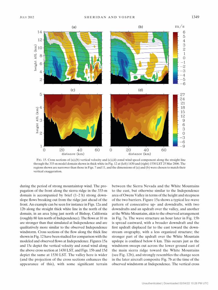
during the period of strong mountaintop wind. The pro-

pagation of the front along the sierra ridge in the 333-m

domain is accompanied by brief (1–2 h) strong down-

slope flows breaking out from the ridge just ahead of the

front. An example can be seen for instance in Figs. 12a and

12b along the straight thick white line in the north of the

domain, in an area lying just north of Bishop, California

(roughly 80 km north of Independence). The flows at 10 m

are stronger than that simulated at Independence and are

qualitatively more similar to the observed Independence

windstorm. Cross sections of the flow along the thick line

shown in Fig. 12 have been studied for comparison with the

modeled and observed flows at Independence. Figures 15a

and 15c depict the vertical velocity and zonal wind along

the above cross section at 1430 LST, and Figs. 15b and 15d

depict the same at 1530 LST. The valley here is wider

(and the projection of the cross sections enhances the

appearance of this), with some significant terrain

between the Sierra Nevada and the White Mountains

to the east, but otherwise similar to the Independence

area of Owens Valley in terms of the height and steepness

of the two barriers. Figure 15a shows a typical lee-wave

pattern of consecutive up- and downdrafts, with two

downdrafts and an updraft over the valley, and another

at the White Mountains, akin to the observed arrangement

in Fig. 7a. The wave structure an hour later in Fig. 15b

is spread eastward, with a broader downdraft and the

first updraft displaced far to the east toward the down-

stream orography, with a less organized structure; the

stronger part of the updraft over the White Mountain

upslope is confined below 6 km. This occurs just as the

windstorm sweeps out across the lower ground east of

the main sierra ridge toward the White Mountains

(see Fig. 12b), and strongly resembles the change seen

in the later aircraft composite Fig. 7b at the time of the

observed windstorm at Independence. The vertical cross

FIG. 15. Cross sections of (a),(b) vertical velocity and (c),(d) zonal wind speed component along the straight line

through the 333-m model domain shown in thick white in Fig. 12 at (left) 1430 and (right) 1530 LST 25 Mar 2006. The

regions shown are narrower than those in Figs. 7 and 11, and the dimensions of (a) and (b) were chosen to match their

vertical exaggeration.



sections of zonal velocity in Figs. 15c and 15d depict how

the strong cross-valley flow sweeps rapidly into the valley,

displacing the up-valley flow (negative zonal velocity)

that existed before 1430 LST to its eastern edge. This

cross-valley flow fills the depth of the valley, unlike that

simulated at Independence. The horizontal wavelength

of the waves subsequently rapidly contracts as the syn-

optic wind strength diminishes (not shown).

To compare the mechanism for the modeled flow

north of Bishop with that simulated at Independence,

profiles at the ridgetop and in the middle of the valley in

the plane shown in Fig. 15 were compared as in Fig. 13

(not shown). Unlike in Fig. 13, there was little contrast

in potential temperature at a given height (typically no

more than 1–2 K). A figure analogous to Fig. 14a is

shown in Fig. 14b for this northern part of the ridge. The

orography present within the lower ground downstream

of the Sierra Nevada here complicates the determination

of the penetration depth of the downslope flow into the

valley, since wind speeds are elevated over the high point

around x 5 33 km in Fig. 15. Therefore, the ‘‘sweeping

out’’ of the valley by the downslope flow, quantified by

xpen in Fig. 14a, is instead represented by the number of

model grid points n12 at which wind speed at 10 m is

greater than 12 m s21, within an area analogous to the

quadrilateral shown in Fig. 9. Meanwhile, hlw represents

the surface height at the lowest point within the above

area where wind speed at 10 m is greater than 12 m s21.

Plotted in Fig. 14b, n12 and hlw appear to be similar to xpen

and hle for Independence in Fig. 14a. Meanwhile, the

similarity of the profiles above ridgetop and valley bot-

tom in this part of ridge mean that the thermal mecha-

nism does not have the same influence here; heq probes

some lower levels only during the onset of the downslope

flow. Possibly the mechanism assists in the initiation of

the flow.

Both the evolution of the modeled lee waves and

downslope flow north of Bishop qualitatively resemble

those measured in the Independence area during the

windstorm, much more than the flow simulated close to

Independence itself. This supports the argument that the

peak in synoptic wind and the approach of the front are

the precursors of the event observed at Independence

and that the more bland behavior in the model at In-

dependence is due to the model not capturing these fea-

tures with the appropriate timing there. It is clear that

what would be judged, on a larger scale, to be fairly minor

synoptic inaccuracies may result in significant errors in

the downslope winds predicted at a given location and

time when modeling complex-terrain flow at high reso-

lution. It is encouraging, however, that a flow similar to

that observed at Independence appears to be simulated

within the model domain around the same time where the

appropriate synoptic factors coincide, suggesting that 1)

a forecast system that is based on a model such as this one

would be able, given an accurate synoptic forecast, to

produce a realistic and representative downslope wind-

storm at Independence and 2) even given synoptic inac-

curacies, the forecast produced would give some warning

of severe windstorms along the ridge. Also, the associa-

tion with the front would mean that surface observations

indicating the front’s progress could be used by fore-

casters to modify predictions of where and when the

severest winds would occur.

6. Conclusions

High-resolution simulations were compared with ob-

servational evidence for the downslope windstorm detected

at Independence during IOP 6 of T-REX. Aircraft

measurements reveal that the windstorm is associated

with large change of phase, wavelength, and amplitude

in the wave system aloft through the depth of the tro-

posphere, coinciding with the arrival of a frontal system

over the sierra during the period of strongest synoptic

winds. Synoptic winds peak earlier in the model, at which

point the front (which lags the observed front) lies a large

distance north of Independence. Downslope winds are

simulated at Independence, but they are weaker and shal-

low foehnlike winds, driven by thermal contrast between

upstream and valley air, and the observed changes of wave

structure are also absent there. Meanwhile, to the north,

windstorms emanate from the ridge across the valley

floor just ahead of the front, linked to a rapid evolution

of the wave structure throughout the depth of the tro-

posphere, in common with the flow observed at Inde-

pendence. It is possible, though, that thermal contrast

between the valley and the ridgetop is still a factor in-

volved in initiating or assisting the development of such

stronger, dynamically forced cases of downslope winds

that occur during the day, such as IOP 6. It is encour-

aging from the point of view of future NWP forecasting

systems that the model correctly predicts strong waves

and downslope winds over Independence while appar-

ently being sensitive to the mechanisms behind the in-

tense IOP-6 windstorm where the appropriate synoptic

conditions are in play. Nevertheless, accurate prediction

of the progress of weather systems and fronts through

large, complex orography such as that of the western

United States is challenging even for numerical models

with very high resolution. Further research is therefore

desirable to understand better the interaction of weather

systems and fronts with significant orography. Mean-

while, research investigating the interaction of ideal-

ized baroclinic systems with both idealized and realistic

terrain would be valuable in establishing the connection



between the particular synoptic features highlighted here

and the intensification of mountain waves, rotors, and

windstorms.

Acknowledgments. The field measurements used were

collected as part of the Terrain-Induced Rotor Ex-

periment and were downloaded from the T-REX Data

Archive, which is maintained by the NCAR Earth

Observing Laboratory (EOL). The primary sponsor of

T-REX is the U.S. National Science Foundation (NSF).

The involvement of the NSF-sponsored Lower At-

mospheric Observing Facilities from the University of

Wyoming and those managed and operated by the NCAR

EOL is acknowledged. The acquisition of the DRI surface

network data was carried out by the DRI team led by Dr.

V. Grubisic. The deployment of this surface network was

funded by NSF Grants ATM-0242886 and ATM-0524891

to DRI. Funding for the car measurements was provided by

Austrian Science Foundation FWF 18940. The acquisition

of the University of Leeds AWS data and radiosonde re-

leases from Independence was done by the University of

Leeds team led by Prof. Stephen Mobbs. The MGAUS

platform and HIAPER aircraft were provided and run by

NCAR. The use of data from the University of Wyoming

King Air is also gratefully acknowledged.

REFERENCES

Agustsson, H., and H. Olafsson, 2007: Simulating a severe wind-

storm in complex terrain. Meteor. Z., 16, 111–122.

Belusic, D., M. Zagar, and B. Grisogono, 2007: Numerical simu-

lation of pulsations in the bora wind. Quart. J. Roy. Meteor.

Soc., 133, 1371–1388.

Billings, B. J., and V. Grubisic, 2008a: A numerical study of the

effects of diurnal heating, moisture, and downstream topog-

raphy on downslope winds within a valley. Preprints, 13th Conf.

on Mountain Meteorology, Whistler, BC, Canada, Amer. Me-

teor. Soc., P2.4. [Available online at http://ams.confex.com/

ams/13MontMet17AP/webprogram/Paper140812.html.]

——, and ——, 2008b: A study of the onset of westerly downslope

winds in Owens Valley. Preprints, 13th Conf. on Mountain Mete-

orology, Whistler, BC, Canada, Amer. Meteor. Soc., 5B.2.

[Available online at http://ams.confex.com/ams/13MontMet17AP/

webprogram/Paper140810.html.]

Chan, P. W., 2009: Atmospheric turbulence in complex terrain:

Verifying numerical model results with observations by remote-

sensing instruments. Meteor. Atmos. Phys., 103, 145–157.

Darby, L. S., and G. S. Poulos, 2006: The evolution of lee-wave–

rotor activity in the lee of Pike’s Peak under the influence of

a cold frontal passage: Implications for aircraft safety. Mon.

Wea. Rev., 134, 2857–2876.

Davies, T., M. J. P. Cullen, A. J. Malcolm, M. H. Mawson,

A. Staniforth, A. A. White, and N. Wood, 2005: A new dy-

namical core for the Met Office’s global and regional mod-

elling of the atmosphere. Quart. J. Roy. Meteor. Soc., 131,1759–1782.

Doyle, J. D., and Coauthors, 2011: An intercomparison of T-REX

mountain-wave simulations. Mon. Wea. Rev., 139, 2811–2831.

Farr, T. G., and Coauthors, 2007: The Shuttle Radar Topography

Mission. Rev. Geophys., 45, RG2004, doi:10.1029/2005RG000183.

Gohm, A., G. Zangl, and G. J. Mayr, 2004: South foehn in the Wipp

Valley on 24 October 1999 (MAP IOP 10): Verification of high-

resolution numerical simulations with observations. Mon. Wea.

Rev., 132, 78–102.

Gregory, D., and P. R. Rowntree, 1990: A mass-flux convection

scheme with representation of cloud ensemble character-

istics and stability-dependent closure. Mon. Wea. Rev., 118,

1483–1506.

Grubisic, V., and J. M. Lewis, 2004: Sierra Wave Project revisited:

50 years later. Bull. Amer. Meteor. Soc., 85, 1127–1142.

——, and B. J. Billings, 2007: The intense lee-wave rotor event of

Sierra Rotors IOP 8. J. Atmos. Sci., 64, 4178–4201.

——, and I. Stiperski, 2009: Lee-wave resonances over double bell-

shaped obstacles. J. Atmos. Sci., 66, 1205–1228.

——, and Coauthors, 2008: The Terrain-Induced Rotor Experi-

ment: A field campaign overview including observational

highlights. Bull. Amer. Meteor. Soc., 89, 1513–1533.

Hastings, D. A., and P. K. Dunbar, Eds., 1999: Global Land One-

Kilometer Base Elevation (GLOBE), digital elevation model,

version 1.0, documentation version 1.0. NOAA/NESDIS/

National Geophysical Data Center Key to Geophysical Re-

cords Doc. 34. 138 pp. [Available online at http://www.ngdc.

noaa.gov/mgg/topo/report/globedocumentationmanual.pdf.]

Holmboe, J. R., and H. Klieforth, 1957: Investigation of mountain

lee waves and the airflow over the Sierra Nevada. UCLA De-

partment of Meteorology Final Rep. for Contract AF 19(604)-

728, 283 pp.

Jiang, Q., and J. D. Doyle, 2008: Diurnal variation of downslope

winds in Owens Valley during the Sierra Rotor Experiment.

Mon. Wea. Rev., 136, 3760–3780.

——, M. Liu, and J. D. Doyle, 2011: Influence of mesoscale dy-

namics and turbulence on fine dust transport in Owens Valley.

J. Appl. Meteor. Climatol., 50, 20–38.

Lock, A. P., A. R. Brown, M. R. Bush, G. M. Martin, and R. N. B.

Smith, 2000: A new boundary layer mixing scheme. Part I:

Scheme description and single-column model tests. Mon. Wea.

Rev., 128, 3187–3199.

Mayr, G. J., and L. Armi, 2010: The influence of downstream di-

urnal heating on the descent of flow across the sierras. J. Appl.

Meteor. Climatol., 49, 1906–1912.

——, J. Vergeiner, and A. Gohm, 2002: An automobile platform

for the measurement of foehn and gap flows. J. Atmos. Oce-

anic Technol., 19, 1545–1556.

Neiman, P. J., F. M. Ralph, R. L. Weber, T. Uttal, L. B. Nance,

and D. H. Levinson, 2001: Observations of nonclassical

frontal propagation and frontally forced gravity waves

adjacent to steep topography. Mon. Wea. Rev., 129, 2633–

2659.

Raab, T., and G. Mayr, 2008: Hydraulic interpretation of the

footprints of Sierra Nevada windstorms tracked with an au-

tomobile measurement system. J. Appl. Meteor. Climatol., 47,

2581–2599.

Ralph, F. M., P. J. Neiman, T. L. Keller, D. Levinson, and L. Fedor,

1997: Observations, simulations, and analysis of nonstationary

trapped lee waves. J. Atmos. Sci., 54, 1308–1333.

Raymond, D. H., 1988: High-order low-pass implicit tangent filters

for use in finite area calculations. Mon. Wea. Rev., 116, 2132–

2141.

Reinecke, P. A., and D. R. Durran, 2009: Initial-condition sensi-

tivities and the predictability of downslope winds. J. Atmos.

Sci., 66, 3401–3418.



Schmidli, J., and Coauthors, 2011: Intercomparison of mesoscale

model simulations of the daytime valley wind system. Mon.

Wea. Rev., 139, 1389–1409.

Smith, R. B., B. K. Woods, J. Jensen, W. A. Cooper, J. D. Doyle,

Q. Jiang, and V. Grubisic, 2008: Mountain waves entering

the stratosphere. J. Atmos. Sci., 65, 2543–2562.

Steenburgh, W. J., C. R. Neuman, and G. L. West, 2009: Discrete

frontal propagation over the Sierra–Cascade Mountains and

intermountain west. Mon. Wea. Rev., 137, 2000–2020.

Stiperski, I., and V. Grubisic, 2011: Trapped lee wave in-

terference in the presence of surface friction. J. Atmos. Sci.,

68, 918–936.

Wilson, D. R., and S. P. Ballard, 1999: A microphysically based

precipitation scheme for the UK Meteorological Office Uni-

fied Model. Quart. J. Roy. Meteor. Soc., 125, 1607–1636.

Woods, B. K., and R. B. Smith, 2010: Energy flux and wavelet di-

agnostics of secondary mountain waves. J. Atmos. Sci., 67,3721–3738.



High-Resolution Simulations of Lee Waves and Downslope ...

Documents

Transcript of High-Resolution Simulations of Lee Waves and Downslope ...