Atmos. Chem. Phys., 10, 83–94, 2010www.atmos-chem-phys.net/10/83/2010/© Author(s) 2010. This work is distributed underthe Creative Commons Attribution 3.0 License.

AtmosphericChemistry

and Physics

High resolution modeling of CO2 over Europe: implications forrepresentation errors of satellite retrievals

D. Pillai1, C. Gerbig1, J. Marshall1, R. Ahmadov2,*, R. Kretschmer1, T. Koch1, and U. Karstens1

1Max Planck Institute for Biogeochemistry, P.O. Box 100164, 07701 Jena, Germany2NOAA Earth System Research Laboratory, Boulder, Colorado, USA* also at: Cooperative Institute for Research in Environmental Sciences, University of Colorado, Boulder, USA

Received: 1 July 2009 – Published in Atmos. Chem. Phys. Discuss.: 30 September 2009Revised: 10 December 2009 – Accepted: 11 December 2009 – Published: 7 January 2010

Abstract. Satellite retrievals for column CO2 with bet-ter spatial and temporal sampling are expected to improvethe current surface flux estimates of CO2 via inverse tech-niques. However, the spatial scale mismatch between re-motely sensed CO2 and current generation inverse modelscan induce representation errors, which can cause system-atic biases in flux estimates. This study is focused on esti-mating these representation errors associated with utilizationof satellite measurements in global models with a horizon-tal resolution of about 1 degree or less. For this we usedsimulated CO2 from the high resolution modeling frameworkWRF-VPRM, which links CO2 fluxes from a diagnostic bio-sphere model to a weather forecasting model at 10×10 km2

horizontal resolution. Sub-grid variability of column aver-aged CO2, i.e. the variability not resolved by global models,reached up to 1.2 ppm with a median value of 0.4 ppm. Sta-tistical analysis of the simulation results indicate that orogra-phy plays an important role. Using sub-grid variability oforography and CO2 fluxes as well as resolved mixing ra-tio of CO2, a linear model can be formulated that couldexplain about 50% of the spatial patterns in the systematic(bias or correlated error) component of representation errorin column and near-surface CO2 during day- and night-times.These findings give hints for a parameterization of represen-tation error which would allow for the representation errorto taken into account in inverse models or data assimilationsystems.

Correspondence to:D. Pillai(kdhanya@bgc-jena.mpg.de)

1 Introduction

Atmospheric CO2 has been rising since pre-industrial timesdue to anthropogenic emissions from fossil fuel combustionand deforestation, which are considered to be major causesof global warming (IPCC, 2007). Climate predictions usingcoupled carbon cycle climate models differ greatly in theirfeedbacks between the biosphere and climate, resulting invastly differing mixing ratios of CO2 at the end of this cen-tury (Friedlingstein et al., 2006). This calls for an improvedunderstanding of biospheric CO2 fluxes at regional scales. Aglobal network of observations is being used together withmodeling tools to derive surface-atmosphere exchanges (viainverse techniques) which can help in quantifying biosphere-climate feedback and assist in monitoring CO2 trends in thecontext of climate change mitigation.

However, past studies show that the current observationnetwork is not sufficient to adequately account for uncertain-ties in surface flux estimates (Gurney et al., 2003). Satel-lite measurements of column-integrated CO2 concentrationswith better spatial and temporal sampling as well as with ade-quate precision (∼1 ppm) are expected to improve this situa-tion (Rayner and O’Brien, 2001; Miller et al., 2007). Passivesatellite missions, such as the Orbiting Carbon Observatory(OCO) (Crisp et al., 2004), and the Greenhouse gases Ob-servatory Satellite (GOSAT) (NIES, 2006) are designed tomeasure column integrated dry air mole fraction under clearsky conditions using reflected sunlight. GOSAT is now inorbit, but unfortunately the launch of OCO failed. In ad-dition, active sensor missions are under investigation, suchas ESA’s Earth Explorer candidate mission A-SCOPE, theAdvanced Space Carbon and Climate Observation of Planet

Published by Copernicus Publications on behalf of the European Geosciences Union.

84 D. Pillai et al.: High resolution modeling of CO2 over Europe

Earth (ESA, 2008) and NASA’s mission ASCENDS, the Ac-tive Sensing of CO2 Emissions over Nights, Days and Sea-sons, which have the advantage of also being able to measureduring the night and thus provide a stronger constraint on res-piration fluxes.

The above mentioned satellite measurements are able toprovide global coverage of column-averaged CO2 dry airmole fraction which can improve current estimates of globalcarbon budgets (via inverse techniques). The footprint sizesof satellite missions using passive sensors (measuring re-flected sun light) such as OCO and GOSAT are approxi-mately 1.3 km and 10.5 km, respectively (Crisp et al., 2004;NIES, 2006). Active missions such as A-SCOPE usingLIDAR technology, have smaller footprint sizes of around0.1 km which allows for better sampling under partiallycloudy conditions by making use of the cloud gaps (ESA,2008). However, active missions need some averaging forthese 0.1 km footprints to improve the signal-to noise. Thesefootprints are at least an order of magnitude smaller than thehighest resolution global inverse models (Peters et al., 2007).

All remote sensing methods to measure atmospheric CO2require clear sky conditions, thus a small footprint is desir-able since it allows sampling during scattered cloud condi-tions. On the other hand, the retrievals may not be represen-tative for average CO2 concentration in such coarse modelgrids, and may thus introduce a larger representation error(a spatial mismatch of satellite retrievals within larger gridcells). The representation error is expected to depend on thestrength and horizontal extent of CO2 flux variability and onmeteorology, both of which influence the variability in atmo-spheric CO2. Previous studies show that the representationerror increases with decreasing horizontal resolution (Ger-big et al., 2003) and is higher when mesoscale circulation isimportant (Tolk et al., 2008; Ahmadov et al., 2007). Basedon measurements from airborne platforms during the CO2Budget and Rectification study (COBRA-2000), Gerbig etal. (2003) concluded that transport models require a horizon-tal resolution smaller than 30 km to capture important spatialvariability of CO2 in the continental boundary layer, whichcould be attributed to the spatial variability of surface fluxes.The representation error corresponding to typical global gridcells can be up to 1 to 2 ppm, which is an order of magnitudelarger than the sampling errors (Gerbig et al., 2003). Thesampling error referred in Gerbig et al. (2003) includes bothlimitations in instrument precision and accuracy and uncer-tainty caused by unresolved atmospheric variability of CO2within the mixed layer due to turbulent eddies. Further, to-pography plays a role in representation error. It is reportedthat representation errors induced by small scale orographicfeatures can be as large as 3 ppm at scales of 100 km (Tolket al., 2008). van der Molen and Dolman (2007), in theircase study around Zotino in Central Siberia, showed that to-pographic heterogeneity of 500 m within a spatial scale of200 km can generate horizontal gradients in CO2 concentra-tions of 30 ppm. Hence it is highly important to address rep-

resentation errors caused by these spatial mismatches, alsofor column-integrated measurements from remote sensing,prior to the quantitative assimilation of the information intoglobal modelling systems.

There are a number of studies which have estimated therepresentation error within a model grid cell when usingsatellite column measurements. Based on high resolutionCO2 simulations, taking the difference between the sim-ulated grid cell mean and the sampled mean, Corbin etal. (2008) estimated the representation error over North andSouth America and concluded that satellite retrievals cannotbe used in current inverse models to represent large regionswith significant CO2 variability unless transport models areto be run at high resolution. Alkhaled et al. (2008) estimatedthe representation error based on statistical methods, usingspatial covariance information of CO2 based on model simu-lation of global CO2 distribution at a spatial scale of 2◦

×2.5◦

over the sampled regions together with information about theretrieved soundings without the knowledge of the true meanvalue. Representation errors are quantified using a hypothet-ical transport model with a spatial resolution of 1◦

×1◦ and a3 km2 retrieval footprint.

This study focuses on estimating possible representationerrors of column mixing ratios from remote sensing in globaltransport models, and on the causes of the spatial variabil-ity of CO2 within a grid cell. Spatial variability of CO2 isassessed quantitatively based on high resolution simulationsfor a domain centered over Europe. Using a high resolu-tion transport model, coupled to surface-atmosphere fluxesof CO2, allows accounting for mesoscale phenomena such asland-sea breeze effects (Ahmadov et al., 2007). Such effectscan not be represented in a statistical method as deployed byAlkhaled et al. (2008). We estimate possible representationerror as the sub-grid variability of near surface CO2 and col-umn averages of CO2 within typical global model grid cells.Hypothetical A-SCOPE track data are used with MODIScloud pixel information to realistically represent satellite ob-servations. In this context it is relevant to see the possibil-ity of a sub-grid parameterization scheme based on resolvedvariables to capture the representation error. Such a parame-terization scheme could pave the way to describing represen-tation error in coarser models without using high resolutionsimulations.

The outline of this paper is as follows: Sect. 2 of this paperprovides a brief overview of the modeling framework whichis used to simulate the CO2 fields. Section 3 presents themethodology adopted to estimate representation error asso-ciated with utilizing satellite column measurements in globalinversion studies. In Sect. 4, we present statistical analy-ses of sub-grid variability of CO2 fields within grid cells of100 km×100 km size to estimate possible representation er-rors for retrieved satellite column mixing ratios and we inves-tigate correlations of sub-grid variability with resolved vari-ables to assess the possibility of parameterization schemesfor representation errors in coarser models.

Atmos. Chem. Phys., 10, 83–94, 2010 www.atmos-chem-phys.net/10/83/2010/

D. Pillai et al.: High resolution modeling of CO2 over Europe 85

Table 1. An overview of the WRF physics/dynamics options used.

Vertical coordinates Terrain-following hydrostatic pressure vertical coordinate

Basic equations Non-hydrostatic, compressibleGrid type Arakawa-C gridTime integration 3rd order Runge-Kutta split-explicitSpatial integration 3rd and 5th order differencing for vertical and horizontal

advection respectively; both for momentum and scalarsDomain configuration 1 domain with horizontal resolution of 10 km;

size 2500×2300 km; 31 vertical levels;Time step 60 sPhysics schemes Radiation – Rapid Radiative Transfer Model (RRTM)

Long wave and Dudhia;Microphysics – WSM 3-class simple ice scheme;Cumulus – Kain-Fritsch (new Eta) scheme (only for thecoarse domain!)PBL – YSU; Surface layer – Monin-ObukhovLand-surface – NOAH LSM

2 Modeling framework

We use the modeling system, WRF-VPRM (Ahmadov et al.,2007), which combines the Weather Research and Forecast-ing model, WRF (http://www.wrf-model.org/), with a diag-nostic biosphere model, the Vegetation Photosynthesis andRespiration Model, VPRM (Mahadevan et al., 2008). Thecoupling of these models is done in such a way that VPRMutilizes near surface temperature (T2) and short wave radia-tion (SNDOWN) from WRF in order to compute CO2 fluxesand to provide these to WRF to be transported as a passivetracer.

The principal component of our modelling system con-sists of a mesoscale transport model, WRF, using the passivetracer transport option from WRF-CHEM (Grell et al., 2005)to simulate the distribution of CO2 transported by advec-tion, convection and turbulence. Some modifications weremade in order to implement simulations of CO2 transport,which are described in detail in Ahmadov et al. (2007). Anoverview of the WRF physics/dynamics options used for oursimulations is given in Table 1.

The satellite-constrained biosphere model, VPRM is usedhere to account for CO2 uptake and emission for differentbiomes. It is a diagnostic model which uses MODIS (http://modis.gsfc.nasa.gov/) satellite indices, the Enhanced Vegeta-tion Index (EVI), and the Land Surface Water Index (LSWI)at 500 m resolution to calculate hourly Net Ecosystem Ex-change (NEE). NEE is calculated here as a sum of GrossEcosystem Exchange (GEE) and Respiration. GEE is calcu-lated by using EVI and LSWI from MODIS, and temperatureat 2 m (T2) and shortwave radiation fluxes (SNDOWN), pro-vided by WRF. Respiration fluxes are calculated as a linearfunction of WRF-simulated temperature (Mahadevan et al.,2008). To represent land cover in VPRM, we used SYNMAPdata (Jung et al., 2006) with a spatial resolution of 1 km and

8 vegetation classes which are suitable for the European do-main. The VPRM parameters which control the CO2-uptakeby photosynthesis and the CO2-emission by respiration foreach vegetation class have been optimized using eddy fluxmeasurements for different biomes in Europe collected dur-ing the CarboEurope IP experiment (for details see Ahmadovet al., 2007). VPRM captures the spatiotemporal variabil-ity of biosphere-atmosphere exchange remarkably well, asshown by comparison with various flux measurements sitescorresponding to different vegetation types for longer peri-ods (Ahmadov et al., 2007; Mahadevan et al., 2008). GEEand respiration computed in VPRM is passed on to WRF tosimulate the distribution of total CO2 concentration.

In addition to VPRM biospheric fluxes, anthropogenic andocean fluxes are included in WRF. High resolution fossilfuel emission data from IER (Institut fur Energiewirtschaftund Rationelle Energieanwendung), University of Stuttgart(http://carboeurope.ier.uni-stuttgart.de/) are used for the year2000, at a spatial resolution of 10 km. Temporal emissionpatterns were preserved by shifting the IER data for 2000 bya few days to match the weekdays in 2003. The total mass ofthe emissions was conserved when mapping onto the WRFgrid. To account for ocean fluxes in WRF, the monthly air-sea fluxes from Takahashi et al. (2002) are used.

Initial and lateral tracer boundary conditions are pre-scribed from global CO2 concentration fields based on asimulation by a global atmospheric Tracer transport model,TM3 (Heimann et al., 2003), with a spatial resolution of4◦

×5◦, and a temporal resolution of 3 h. TM3 is drivenby re-analyzed meteorological data from NCEP and surfacefluxes optimized by atmospheric inversion (Rodenbeck etal., 2003). As initial and lateral meteorological boundaryconditions for WRF, analyzed fields from ECMWF (http://www.ecmwf.int/) with a horizontal resolution of approxi-mately 35 km and a 6-h time step are used. The model setup

www.atmos-chem-phys.net/10/83/2010/ Atmos. Chem. Phys., 10, 83–94, 2010

86 D. Pillai et al.: High resolution modeling of CO2 over Europe

−20

-

10

0

10

20

3

0

(a) (b)

02

412

106

8

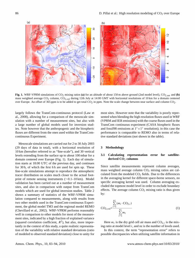
Fig. 1. WRF-VPRM simulations of CO2 mixing ratios(a) for an altitude of about 150 m above ground (2nd model level), CO2,sur and(b)mass weighted average CO2 column, CO2,col during 12th July at 14:00 GMT with horizontal resolutions of 10 km for a domain centeredover Europe. An offset of 365 ppm is to be added to get total CO2 in ppm. Note the scale change between near surface and column CO2.

largely follows the TransCom-continuous protocol (Law etal., 2008), allowing for a comparison of the mesoscale sim-ulation with a number of measurement sites, but also witha large number of global models used for inversion stud-ies. Note however that the anthropogenic and the biosphericfluxes are different from the ones used within the TransCom-continuous Experiment.

Mesoscale simulations are carried out for 2 to 30 July 2003(29 days of data in total), with a horizontal resolution of10 km (hereafter referred to as “fine-scale”), and 30 verticallevels extending from the surface up to about 100 mbar for adomain centered over Europe (Fig. 1). Each day of simula-tion starts at 18:00 UTC of the previous day, and continuesfor 30 h, of which the first 6 h are used for spin up. Thesefine-scale simulations attempt to reproduce the atmospherictracer distribution on scales much closer to the actual foot-print of remote sensing instruments (∼0.1–10 km). Modelvalidation has been carried out at a number of measurementsites, and also in comparison with output from TransCommodels which are used for global inversion studies. Table 2shows a summary of statistics of the WRF-VPRM simu-lation compared to measurements, along with results fromtwo other models used in the TransCom-continuous Experi-ment, the global model TM3 and the regional model REMO(Chevillard et al., 2002). WRF-VPRM performs reasonablywell in comparison to other models for most of the measure-ment sites, indicated by a high fraction of explained variance(squared correlation coefficient,R2), but also, more impor-tantly in the context of this study, a quite realistic representa-tion of the variability with relative standard deviations (ratioof modeled to observed standard deviation) close to unity for

most sites. However note that the variability is poorly repre-sented when blending the high resolution fluxes used in WRF(VPRM and IER emissions) with the coarse fluxes used in theTransCom continuous experiment (CASA biospheric fluxesand fossil98 emissions at 1◦

×1◦ resolution); in this case theperformance is comparable to REMO also in terms of rela-tive standard deviations (not shown in the table).

3 Methodology

3.1 Calculating representation error for satellite-derived CO2 columns

Since satellite measurements represent column averages,mass weighted average column CO2 mixing ratios are cal-culated from the modeled CO2 fields. Due to the differencesin the averaging kernel for different space-borne sensors, nospecific averaging kernel was used. Column averaging ex-cluded the topmost model level in order to exclude boundaryeffects. The average column CO2 mixing ratio is thus givenby:

CO2,col=

nz∑i=1

(mi ·CO2,i)

nz∑i=1

mi

(1)

Heremi is the dry grid cell air mass and CO2,i is the mix-ing ratio at model leveli, and nz is the number of levels used.

In this context, the term “representation error” refers topossible discrepancies when utilizing satellite information in

Atmos. Chem. Phys., 10, 83–94, 2010 www.atmos-chem-phys.net/10/83/2010/

D. Pillai et al.: High resolution modeling of CO2 over Europe 87

current global models, due to the spatial scale mismatchesbetween satellite retrievals and larger model grids. Repre-sentation error (σc,col) is thus estimated for every time step(hourly) as sub-grid variability (standard deviation of fine-scale CO2,col) within the spatial resolution of current globalmodels. The spatial scale of 100 km is chosen to representthe lower limit of grid cell size found in global models usedfor inversions. The calculated column averages do not in-clude the entire stratosphere, which amounts to a fractionof 10% of the total atmospheric column (pressure at modeltop is 100 mbar). Since horizontal variability of CO2 in thestratosphere on scales below 100 km is small (at least notlarger than in the troposphere), neglecting this part of the col-umn might thus result at maximum in a 10% overestimationof the sub-grid variability.

The monthly averagedσc,col (i.e.,c,col, specific for a givenhour of the day) includes random and systematic compo-nents of representation errors. It is important to assess whichcomponent of this representation error is purely random, i.e.noise introduced by weather, and which part is systematicin nature (the “bias”, or “correlated error” term). Random,uncorrelated errors are expected to decrease when averagingover longer time periods, e.g. for deriving monthly fluxes. Inorder to exclude random errors, daily values of CO2 mixingratios (at a specific time, e.g. 14:00 GMT) are averaged forthe whole month and subsequently estimated sub-grid vari-ability from this averaged concentration (i.e.,σ2,col). Thisgives a representation error (σc,col(bias)) that is purely of sys-tematic nature on a monthly time scale. We define the term“bias” introduced here as the part of the error that is corre-lated over the timescale of a month. Note that the bias com-ponent of error is always denoted with subscript “(bias)”.

In addition to σc,col, near-surface CO2 mixing ratios(CO2,sur) at an altitude of about 150 m above the surface (thesecond model level) are also analyzed in terms of sub-gridvariability σc,sur. A similar analysis is again carried out for aspatial resolution of 200 km (not shown).

3.2 Using A-SCOPE track information includingMODIS cloud information

In order to realistically represent satellite retrievals with ourmodel simulations, we followed the simulated A-SCOPEsampling track. Temporal resolution of the track is 0.5 s, cor-responding to a spatial distance between subsequent samplesof 3.5 km (F. M. Breon, Laboratoire des Sciences du Climatet de l’Environnement, personal communication). The sam-ples are initially aggregated to a horizontal resolution 10 kmand these 10 km samples are used for further analysis. Notethat this aggregation causes the representation error to be un-derestimated. Since satellite retrievals require clear sky con-ditions, the simulations are sampled for the pixels with clearsky. Cloud free conditions are picked up based on MODIScloud pixel information (http://modis-atmos.gsfc.nasa.gov/MOD35 L2/index.html) at 1 km resolution for the period of

Table 2. Statistics for the comparison of WRF-VPRM simulationsto measurements, along with results from two transport models usedin the TransCom Continuous experiment.

Squared correlation coefficient,R2

Model [Horizontal Resolution]

Station WRF-VPRM REMO TM3vfg[10×10 km2] [0.5◦

×0.5◦] [1.875◦×1.875◦]Heidelberg 0.29 0.48 0.37Hegyhatsal 48m 0.44 0.35 0.28Hegyhatsal 115 0.41 0.48 0.25Schauinsland 0.16 0.07 0.06Mace Head 0.24 0.48 0.29Monte Cimone 0.38 0.13 0.17

Ratio of modeled to measured standard deviation

Model [Horizontal Resolution]

Station WRF-VPRM REMO TM3vfg[10×10 km2] [0.5◦

×0.5◦] [1.875◦×1.875◦]Heidelberg 0.95 2.72 1.03Hegyhatsal 48m 1.21 2.75 1.64Hegyhatsal 115 1.19 1.61 1.28Schauinsland 0.99 0.92 0.82Mace Head 0.6 1.02 0.79Monte Cimone 1.82 0.65 0.79

simulation. 46 438 samples of cloud free columns are ex-tracted including 27 605 samples (60%) over land. Thesesamples were aggregated to a spatial scale of 100 km alongthe A-SCOPE track. There is an average of 6.6 cloud free10 km samples along the A-SCOPE track within each 100 kmgrid cell. The representation error for A-SCOPE derivedCO2 columns (σascope) is calculated as the standard devia-tions of the difference of 100 km×100 km flight track aver-ages using only A-SCOPE 10 km samples along the flighttrack, and the 100 km×100 km averages based on all 10 kmgrid cells (σ [A-SCOPE 100 km averages – true 100 km av-erages]).

4 Results and discussion

In this section the results based on WRF-VPRM simulationsof the distribution of atmospheric CO2 in July 2003 are pre-sented. An example of the WRF-VPRM output is given inFig. 1, showing simulated (a) CO2,sur and (b) CO2,col on 12July at 14:00 GMT. Strong spatial variability of the boundarylayer CO2 can be seen near the coasts (Fig. 1a) due to the 3-D-rectification effect (the temporal covariance between sea-land breeze transport and biosphere-atmosphere fluxes, bothof which are radiation controlled) (Ahmadov et al., 2007),which causes respired CO2 to be advected over the ocean bysynoptic winds or by the land-breeze circulation and to beconcentrated in a shallow layer due to the lack of verticalmixing over the ocean. There is also strong variability asso-ciated with frontal activity towards the north-eastern edge of

www.atmos-chem-phys.net/10/83/2010/ Atmos. Chem. Phys., 10, 83–94, 2010

88 D. Pillai et al.: High resolution modeling of CO2 over Europe

01

23

45

6

(a)

0.0

0.2

0.4

0.6

0.8

1.0

1.2

(b)

Fig. 2. The monthly averaged subgrid variability of CO2 concentrations for:(a) near-surface,σc,sur and(b) column average,σc,col, for July2003, using 14:00 GMT only. All values are in ppm.

0 2 4 6 8 10 12

(0,2

]

(4,6

]

(8

,10]

(12,

14]

σc [ppm]

Alti

tude

[km

]

Fig. 3. Box and whisker plot for different altitudes (from ground)ranges of the sub-grid concentration variability (σc) for July 2003(14:00 GMT only). Boxes indicate the central 50%, the bar acrossthe box is the median value, and whiskers indicate the range of thecentral 95% of data points. Individual data points are shown outsidethe central 95%.

the domain, with strong gradients in CO2 associated with thelocation of a cold front. Such behavior has previously beenreported (Parazoo et al., 2008), and has been attributed to thedeformational flow along the fronts. A similar pattern is fol-lowed in the CO2 column average (Fig. 1b) near coasts aswell as towards the north-eastern edge of the domain, whichsuggests a strong contribution of boundary layer concentra-

tions to column averages. Movies showing the complete sim-ulation can be seen at:

http://www.bgc.mpg.de/bgc-systems/news/near-surfaceco2.html and http://www.bgc.mpg.de/bgc-systems/news/columnco2.html

4.1 Subgrid variability of near surface and column av-erages of CO2 concentrations

Figure 2 shows the monthly averagedσc,sur and σc,col (at14:00 GMT only) for July 2003. Coastal and mountain re-gions are distinct, with strong sub-grid variability both innear surface and in column averages of CO2 concentrations.This is due to relatively strong gradients of surface fluxes inthese regions.

The similarity in spatial patterns ofσc,col and σc,sur(Fig. 2a and b) indicates that the CO2 column values arecorrelated with surface values. Figure 3 shows the profiledistribution of monthly averaged (at 14:00 GMT)σc withindifferent bins of vertical model levels. Most of the higher val-ues ofσc are found to be within the lowest 2 km.σc stronglydecreases with increasing altitude, showing less influence ofsurface fluxes at higher altitudes. These results are consis-tent with van der Molen and Dolman (2007) which showsthat the effect of surface heterogeneity is generally observedin lower atmospheric layers. This indicates the dominanceof boundary layer concentration variability in column aver-ages. These dominances can be significant during synopticscale events, where CO2 column variability is strongly corre-lated (squared correlation coefficient,R2=0.37) to boundarylayer concentrations (see Fig. 1), but not strongly correlated(squared correlation coefficient,R2=0.12) to concentrationsin the free troposphere around 4 km (not shown).

Atmos. Chem. Phys., 10, 83–94, 2010 www.atmos-chem-phys.net/10/83/2010/

D. Pillai et al.: High resolution modeling of CO2 over Europe 89

0.2

0.4

0.6

0.8

1.0

1.2

0.0

-

Fig. 4. The monthly averaged subgrid variability of temporally ag-gregated CO2 column averages (bias) [ppm] for July 2003, using14:00 GMT only.

The analysis shows that the monthly averagedσc,col forthe domain is, on average, 0.4 ppm, with maximum valuesaround 1.2 ppm and the 90% percentile 0.6 ppm (see Fig. 2).Partitioning the data into ocean and land pixels shows thatσc,col is more than twice as large over land (0.5 ppm) as com-pared to over ocean areas (0.2 ppm) as is expected due to thestronger magnitude and variability of terrestrial fluxes. Thisis not negligible compared to the targeted accuracy of fu-ture satellite retrievals. The monthly bias error,σc,col(bias), issmaller than the full error, but shows a similar pattern withmaximum values around 0.9 ppm for mountain and coastalregions (Fig. 4).

4.2 Representation error for satellite derived CO2columns

4.2.1 Hypothetical satellite track

Representation errors are quantified here using a hypotheti-cal satellite track going through each 100 km×100 km cell.Following the sampling conditions used by Alkhaled etal. (2008) (hereafter referred to as A08), we assumed twospatial distributions of satellite retrievals: (1) a full North-South swath (10 pixels from south to north) in each grid cell(idealized sampling condition), and (2) a single retrieval atthe corner of each grid cell (adverse sampling condition).The representation errors of hypothetical satellite-derivedCO2 columns (σhypo) are estimated for these two spatial dis-tributions of satellite retrievals within each 100 km×100 kmgrid cell. Figure 5 shows the distribution ofσhypo for a fullNorth-South swath at the center of each 100×100 km gridcell. Theσhypo for the previously mentioned sampling con-

0.0

0.2

0.4

0.6

0.8

1.0

1.2

Fig. 5. The subgrid variability of column averages of CO2 con-centrations [ppm] based on hypothetical north-south swath at thecenter of each 100 km grid cell for July 2003 (monthly averaged at14:00 GMT).

ditions are estimated and compared with A08 in July for theEuropean domain, and are given in Table 3. The larger rep-resentation errors are seen over land for both sampling con-ditions, and are about a factor of two larger when comparedto ocean (see Table 3). The statistical approach suggested byA08 gives much smoother behaviour compared to our resultsand also neglects land-ocean differences in the European do-main. Under idealized sampling conditions (10 pixel swath),the representation error estimates are nearly an order of mag-nitude larger than those by A08, and under adverse samplingconditions (single corner pixel) our estimates are a factor oftwo larger compared to those provided by A08 (Table 3).

This finding is in line with experimental evidence: A08found agreement between their estimates and observation-based estimates from Lin et al. (2004), however the latterwere a conservative (low-end or lower limit) estimate of sub-grid variability. In fact the power variogram model used byLin et al. (2004) underestimated the observed variogram es-timates by a factor of 3 to 5 at scales smaller than 200 km(see Fig. 2 in Lin et al. (2004)). This corresponds to abouta factor two differences in single pixel representation error,which is remarkably similar to the factor found between thehigh-resolution model based estimate and the one providedby A08. This suggests that it is not generally possible to ex-tract information about the representation error from coarsemodel simulations as suggested in A08. Such a method islikely to fail in cases of mesoscale complexity.

www.atmos-chem-phys.net/10/83/2010/ Atmos. Chem. Phys., 10, 83–94, 2010

90 D. Pillai et al.: High resolution modeling of CO2 over Europe

Table 3. The possible representation error when using A-SCOPEand hypothetical satellite tracks for different sampling conditions.The values given in square brackets indicate monthly bias compo-nent. All values are in ppm.

Representation error All Land Ocean Alkhaled et al. (2008),EU domain∗

Hypothetical Satellite 0.59 0.72 0.35 0.30–0.40(Single corner pixel) [0.22] [0.28] [0.09]

Hypothetical Satellite 0.38 0.46 0.24 0.04–0.06(North-South Swath) [0.16] [0.20] [0.05]

ASCOPE 0.34 0.39 0.30[0.12] [0.15] [0.08]

∗ extracted from Alkhaled et al. (2008), Fig. 2c and d forour domain.

4.2.2 A-SCOPE 100 km averages

σascopeis evaluated using the A-SCOPE satellite track infor-mation as described in Sect. 3.2. When combining all A-SCOPE samples within each 100 km grid cell, the resultingrepresentation errorσascopeis reduced compared to the sin-gle pixel error. Note that this is due to the fact that severalpixels contribute to each A-SCOPE sample, whose error canpartially cancel out. As for the hypothetical satellite tracks,larger representation errors for A-SCOPE are seen over land(0.4 ppm) as compared to over ocean areas (0.3 ppm) (Ta-ble 3).

4.3 Dependence of representation error on explanatoryvariables

Knowledge about the size and the spatial and temporal pat-terns of the representation error is expected to improve in-verse modeling of satellite data, but this would involve usinga high resolution model to estimate the representation error.Our goal is to construct a linear model based on a subsetof those explanatory variables which explains a significantfraction of sub-grid variability, and which can be used in thecontext of global inverse modelling to capture the spatiotem-poral patterns. Such a linear model is the simplest subgridparameterization scheme for representation errors in coarsermodels, only accounting for local effects and neglecting anyeffects from advection of subgrid variability.

Statistical relationships between the representation errorand the following variables are explored (not shown): thestandard deviation of the fluxes (σf ), the mean of the fluxes(f ), the absolute mean of the fluxes (|f |), the mean terrainheight (h), standard deviation of the terrain heights (σh) andthe mean mixing ratio near the surface (c). c is includedsince it can be expected that variability is associated with themagnitude of the mixing ratios. The analysis showed that therepresentation error is best explained by the variablesσh, σf

Table 4. The statistical estimation (squared correlation coefficient)of the bias component of the representation error (σc(bias)) ex-plained by each variable and the proposed linear model.

ExplanatoryDay-time Night-time

Variables

Column Surface Column Surfaceσc,col σc,sur σc,col σc,sur

σf 0.34 0.66 0.09 0.13[µ.moles/m2 s−1]σh 0.51 0.20 0.59 0.33[m]c 0.18 0.09 0.02 0.16[ppm]

Linear model with 0.63 0.67 0.63 0.46σf , σh & c

and c during day-time as well as night-time. Hence a lin-ear model is constructed using three variables:σh, σf andc.Table 4 gives the statistical estimation of the variability ex-plained by each of these variables. In addition toσc,col, wealso investigated the same linear model forσc,sur. The ex-plained variability by each of these variables differs betweenday- and night-time, also between column and near-surfacemixing ratios. The proposed linear model has the same vari-able structure, but different coefficients for the explanatoryvariables.

Figure 6 shows the dependence ofσc,col(bias) on each ofthese variables. Figure 6a shows a monotonic increase ofσc,col(bias) with increasingσf at the 100 km scale and ex-plains 34% ofσc,col(bias) during day-time, however the re-lationship withσf is absent during night-time (Fig. 6d). It isfound in general thatσc(bias) is well explained byσf (34% ofthe total column variability and 66% of the surface variabil-ity) during day-time; however correlations are weaker duringnight-time (Table 4). This can be explained as follows: thefluxes are larger and more spatially variable during daytimethan during nighttime. In addition, strong vertical mixingduring day-time couples the mixing ratios over a deeper partof the column to the patterns in surface fluxes, while duringnight there is less vertical mixing, with more advection anddrainage flow in the stable nocturnal boundary layer, smear-ing out the signatures from patchy surface fluxes.

The effect of heterogeneity in topography onσc,col(bias)can be seen in Fig. 6b and e.σc,col(bias) increases in responseto increase inσh and explains good fraction (51–59%) of sub-grid variability of mixing ratios. Nocturnalσc,sur(bias) is morecorrelated withσh (33%), rather than day-timeσc,sur(bias)(20%) (see Table 4; not shown the figure). This shows thattopography has more influence on representation error ofCO2 concentrations in the lower boundary layer during nightwhen transport is more dominant than surface flux variabil-ity.

Atmos. Chem. Phys., 10, 83–94, 2010 www.atmos-chem-phys.net/10/83/2010/

D. Pillai et al.: High resolution modeling of CO2 over Europe 91

(0,1] (2,3] (4,5] (6,7] (8,9]

day−time , R² : 0.34

(0,90] (270,360] (540,630]

day−time , R² : 0.51

(0,1] (3,4] (6,7] (9,10]

day−time , R² : 0.18

σc[p

pm]

(0,0.1] (0.6,0.7] (1.2,1.3]

σf [μ.moles/m sec ]

night−time , R² : 0.09

(0,90] (270,360] (540,630]

σh [m]

night−time , R² : 0.59

(0,2] (4,6] (8,10] (14,16]

c

night−time , R² : 0.02

σc[p

pm]

[ppm]-

(a) (b) (c)

(d) (e) (f )

2 -1

00.1

0.2

0.3

0.4

0.5

0.6

0.7

00.1

0.2

0.3

0.4

0.5

0.6

0.7

00.1

0.2

0.3

0.4

0.5

0.6

0.7

00.2

0.4

0.6

0.8

00.2

0.4

0.6

0.8

00.2

0.4

0.6

0.8

Fig. 6. Distribution of the bias component of column CO2 sub-grid variability (σc,col(bias)) on (a, d) σf , (b, e) σh, (c, f) c for July 2003[(a)–(c): 14:00 GMT only, (d)–(f): 02:00 GMT only]. Boxes indicate the central 50%, the bar across the box the median, and whiskers thecentral 95%. Individual data points are shown outside the central 95%.

c is negatively correlated withσc,col(bias) during day-time(see Table 5) and explains 18% of variability, whereas thecorrelation is absent during night-time (Fig. 6c and f). Incontrast to this, the correlation ofc with σc,surl(bias) is absentduring day-time, but explains 16% of nocturnal variability(Table 4).

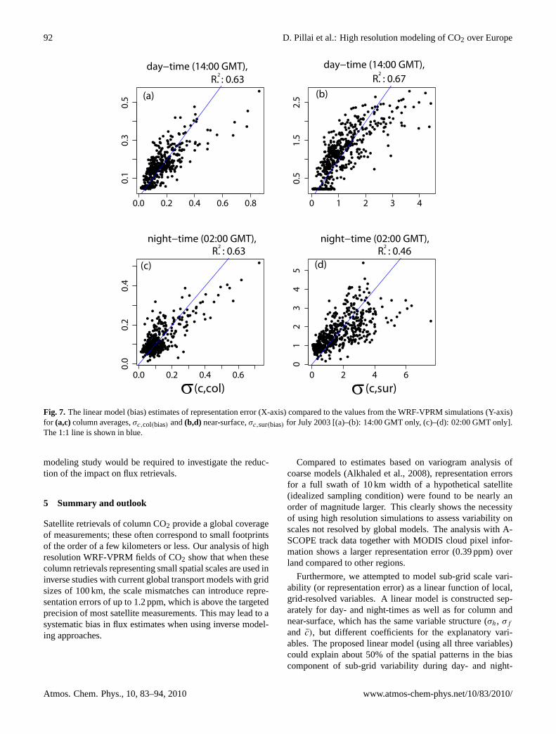
The linear model using all three variables explains about50% of the spatial patterns in the (monthly) bias componentof sub-grid variability during day- and night-times (Table 4).It is found that nocturnalσc,sur is better explained (60% incomparison to 46%) by the linear model when including thevariable f , however no further improvements forσc,col orday-timeσc,sur are found (not shown). Figure 7 illustrateshow well the representation error is captured with the pro-posed linear model. It seems therefore possible to introducethis parameterization of representation error in coarser mod-els so that data assimilation systems using coarser transportmodels can use realistic estimates for representation errorsthat have the appropriate spatial and temporal dependence.

Table 5 gives the linear model coefficients for each of theseexplanatory variables. Note that coefficients are horizontalscale dependent, and we expect them to also vary betweenseasons due to differences in flux patterns and transport char-acteristics.

The implementation of the proposed parameterizationscheme in global models requires these three explanatoryparameters: σh can be easily calculated from any highresolution topographic elevation data, for example USGSGTOPO dataset (http://eros.usgs.gov/#/FindData/ProductsandDataAvailable/GTOPO30). The information on fluxes(σf ) can be accessed from biosphere models with high spa-tial resolution, e.g. VPRM.c is represented in global modelsimulations or from the satellite retrievals. However, care hasto be taken to remove long term trends and seasonal cycleswhen simulating longer periods, otherwise representation er-ror estimates would be falsely influenced by these. Sucha simple parameterization would likely reduce the impactof representation errors significantly, although an inverse

www.atmos-chem-phys.net/10/83/2010/ Atmos. Chem. Phys., 10, 83–94, 2010

92 D. Pillai et al.: High resolution modeling of CO2 over Europe

0.0 0.2 0.4 0.6 0.8

0.1

0.3

0.5

day−time (14:00 GMT),R. : 0.63

0 1 2 3 4

0.5

1.5

2.5

day−time (14:00 GMT), R. : 0.67

a

0.0 0.2 0.4 0.6

0.0

0.2

0.4

σ(c,col)

night−time (02:00 GMT), R. : 0.63

0 2 4 6

01

23

45

σ (c,sur)

night−time (02:00 GMT), R. : 0.46

f

(a) (b)

(c) (d)

2 2

2 2

Fig. 7. The linear model (bias) estimates of representation error (X-axis) compared to the values from the WRF-VPRM simulations (Y-axis)for (a,c)column averages,σc,col(bias) and(b,d) near-surface,σc,sur(bias) for July 2003 [(a)–(b): 14:00 GMT only, (c)–(d): 02:00 GMT only].The 1:1 line is shown in blue.

modeling study would be required to investigate the reduc-tion of the impact on flux retrievals.

5 Summary and outlook

Satellite retrievals of column CO2 provide a global coverageof measurements; these often correspond to small footprintsof the order of a few kilometers or less. Our analysis of highresolution WRF-VPRM fields of CO2 show that when thesecolumn retrievals representing small spatial scales are used ininverse studies with current global transport models with gridsizes of 100 km, the scale mismatches can introduce repre-sentation errors of up to 1.2 ppm, which is above the targetedprecision of most satellite measurements. This may lead to asystematic bias in flux estimates when using inverse model-ing approaches.

Compared to estimates based on variogram analysis ofcoarse models (Alkhaled et al., 2008), representation errorsfor a full swath of 10 km width of a hypothetical satellite(idealized sampling condition) were found to be nearly anorder of magnitude larger. This clearly shows the necessityof using high resolution simulations to assess variability onscales not resolved by global models. The analysis with A-SCOPE track data together with MODIS cloud pixel infor-mation shows a larger representation error (0.39 ppm) overland compared to other regions.

Furthermore, we attempted to model sub-grid scale vari-ability (or representation error) as a linear function of local,grid-resolved variables. A linear model is constructed sep-arately for day- and night-times as well as for column andnear-surface, which has the same variable structure (σh, σf

and c), but different coefficients for the explanatory vari-ables. The proposed linear model (using all three variables)could explain about 50% of the spatial patterns in the biascomponent of sub-grid variability during day- and night-

Atmos. Chem. Phys., 10, 83–94, 2010 www.atmos-chem-phys.net/10/83/2010/

D. Pillai et al.: High resolution modeling of CO2 over Europe 93

Table 5. Coefficients of the linear model for the monthly bias component of the representation error (σc(bias)). The standard errors of thecoefficients are given in curly brackets.

Day-time Night-time

Column Surface Column Surfaceσc,col σc,sur σc,col σc,sur×10−2

×10−2×10−2

×10−2

Resolution 100 200 100 200 100 200 100 200[km×km]

σf 1.2 1.7 26.5 34.1 −0.01 0.81 12.6 28.6[µ.moles/m2 s−1] {0.15} {0.32} {1.03} {2.00} {0.60} {1.35} {10.17} {18.91}

σh 0.04 0.04 0.07 0.05 0.05 0.05 0.50 0.40[m] {0.00} {0.00} {0.02} {0.03} {0.00} {0.00} {0.03} {0.05}

c −0.47 −0.40 0.38 0.10 −0.58 −0.91 16.2 17.4[ppm] {0.07} {0.16} {0.47} {1.02} {0.09} {0.23} {1.50} {3.26}

Intercept 8.5 11.6 19.3 26.7 10.9 17.1 −27 −18[ppm] {0.58} {1.58} {4.16} {9.85} {0.77} {2.04} {13.05} {28.64}

times. These findings suggest a parameterization whichwould enable a substantial fraction of the representation errorto be taken into account more quantitatively.

Future steps are to implement this parameterization in aninverse modeling system and to assess, using pseudo-data ex-periments, to what degree biases in retrieved fluxes due torepresentation errors can be avoided. A further refinement ofthe method will be to treat the subgrid variance as a traceritself, allowing for advection of subgrid variance within thecoarse transport models similar to the study by Galmarini etal. (2008), with the difference that the focus is not on micro-scale, but rather on mesoscale variability. This would prob-ably allow to better describing the representation error overthe ocean near the coasts, which with the current linear (lo-cal) model cannot be described. When including such a re-alistic description of the representation error into a data as-similation system that uses remotely-sensed column CO2, weexpect that the retrieved information, such as regional carbonbudgets and uncertainties thereof, will improve significantly.

Acknowledgements.This work has been supported through Euro-pean Space Agency funding (contract AO/1-5244/06/NL/HE). Theauthors thank Francois-Marie Breon for providing the algorithm tocalculate the A-SCOPE track and to select cloud free pixels.

The service charges for this open access publicationhave been covered by the Max Planck Society.

Edited by: F. Dentener

References

Ahmadov, R., Gerbig, C., Kretschmer, R., Koerner, S., Neininger,B., Dolman, A. J., and Sarrat,C.: Mesoscale covarianceof transport and CO2 fluxes: Evidence from observationsand simulations using the WRF-VPRM coupled atmosphere-biosphere model, J. Geophys. Res.-Atmos., 112, D22107,doi:22110.21029/22007JD008552, 2007.

Alkhaled, A. A., Michalak, A. M., and Kawa, S. R.: Us-ing CO2 spatial variability to quantify representation errorsof satellite CO2 retrievals, Geophys. Res. Lett., 35, L16813,doi:10.1029/2008GL034528, 2008.

Chevillard, A., Karstens, U., Ciais, P., Lafont, S., and Heimann, M.:Simulation of atmospheric CO2 over Europe and western Siberiausing the regional scale model REMO, Tellus B, 54B, 872–894,2002.

Corbin, K. D., Denning, A. S., Lu, L., Wang, J.-W., and Baker,I. T.: Possible representation errors in inversions of satel-lite CO2 retrievals, J. Geophys. Res.-Atmos., 113, D02301,doi:10.1029/2007JD008716, 2008.

Crisp, D., Atlas, R. M., Breon, F.-M., Brown, L. R., Burrows, J. P.,Ciais, P., Connor, B. J.,Doney, S. C., Fung, I. Y., Jacob, D. J.,Miller, C. E., O’Brien, D., Pawson, S., Randerson, J.T., Rayner,P., Salawitch, R. J., Sander, S. P., Sen, B., Stephens, G. L., Tans,P. P., Toon, G. C., Wennberg, P. O., Wofsy, S. C., Yung, Y. L.,Kuang, Z., Chudasama, B., Sprague, G.,Weiss, B., Pollock, R.,Kenyon, D., and Schroll, S.: The Orbiting Carbon Observatory(OCO) mission, Adv. Space Res., 34, 700–709, 2004.

ESA: European Space Agency Mission Assessment Reports-ASCOPE, online available at:http://esamultimedia.esa.int/docs/SP1313-1ASCOPE.pdf, 2008.

Friedlingstein, P., Cox, P., Betts, R., Bopp, L., von Bloh, W.,Brovkin, V., Cadule, P., Doney, S., Eby, M., Fung, I., Bala, G.,

www.atmos-chem-phys.net/10/83/2010/ Atmos. Chem. Phys., 10, 83–94, 2010

94 D. Pillai et al.: High resolution modeling of CO2 over Europe

John, J., Jones, C., Joos, F., Kato, T., Kawamiya, M., Knorr,W.,Lindsay, K., Matthews, H. D., Raddatz, T., Rayner, P., Re-ick, C., Roeckner, E., Schnitzler, K.-G., Schnur, R., Strassmann,K., Weaver, A. J., Yoshikawa, C., and Zeng, N.: Climate carboncycle feedback analysis: Results from the C4MIP model inter-comparison, J. Climate, 19, 3337–3353, 2006.

Galmarini, S., Vinuesa, J.-F., and Martilli, A.: Modeling the impactof sub-grid scale emission variability on upper-air concentration,Atmos. Chem. Phys., 8, 141–158, 2008,http://www.atmos-chem-phys.net/8/141/2008/.

Gerbig, C., Lin, J. C., Wofsy, S. C., Daube, B. C., Andrews, A.E., Stephens, B. B., Bakwin, P. S., and Grainger, C. A.: To-ward constraining regional-scale fluxes of CO2 with atmosphericobservations over a continent: 1. Observed spatial variabilityfrom airborne platforms, J. Geophys. Res.-Atmos., 108, 4756,doi:4710.1029/2002JD003018, 2003.

Grell, G. A., Peckham, S. E., Schmitz, R., McKeen, S. A., Frost, G.,Skamarock, W. C., and Eder, B.: Fully coupled online chemistrywithin the WRF model, Atmos. Environ., 39, 6957–6975, 2005.

Gurney, K. R., Law, R. M., Denning, A. S., Rayner, P. J., Baker,D., Bousquet, P., Bruhwiler, L., Chen, Y.-H., Ciais, P., Fan, S.M., Fung, I. Y., Gloor, M., Heimann, M., Higuchi, K., John, J.,Kowalczyk, E., Maki, T., Maksyutov, S., Peylin, 5 P., Prather, M.,Pak, B. C., Sarmiento, J., Taguchi, S., Takahashi, T., and Yuen,C.-W.: TransCom 3 CO2 inversion intercomparison: 1. Annualmean control results and sensitivity to transport and prior fluxinformation, Tellus B, 55, 555–579, 2003.

Heimann, M., Koerner, S., Tegen, I., and Werner, M.: The globalatmospheric tracer model TM3, Max-Planck Institut fur Biogeo-chemie, Technical Reports 5, 131 pp., 2003.

IPCC: Climate Change 2007: Synthesis Report. Contribution ofWorking Groups I, II and III to the Fourth Assessment Reportof the Intergovernmental Panel on Climate Change, edited by:Core Writing Team, Pachauri, R. K., and Reisinger, A., IPCC,Cambridge University Press, Cambridge, 104 pp., 2007.

Jung, M., Henkel, K., Herold, M., and Churkina, G.: Exploitingsynergies of global land cover products for carbon cycle model-ing, Remote Sens. Environ., 101, 534–553, 2006.

Law, R. M., Peters, W., R¨odenbeck, C., Aulagnier, C., Baker,I., Bergmann, D. J., Bousquet, P., Brandt, J., Bruhwiler, L.,Cameron-Smith, P. J., Christensen, J. H., Delage, F., Denning,A. S., Fan, S., Geels, C., Houweling, S., Imasu, R., Karstens, U.,Kawa, S. R., Kleist, J., Krol, M. C., Lin, S.-J., Lokupitiya, R.,Maki, T., Maksyutov, S., Niwa, Y., Onishi, R., Parazoo, N., Pa-tra, P. K., Pieterse, G., Rivier, L., Satoh, M., Serrar, S., Taguchi,S., Takigawa, M., Vautard, R., Vermeulen, A. T., and Zhu, Z.:TransCom model simulations of hourly atmospheric CO2: Ex-perimental overview and diurnal cycle results for 2002, GlobalBiogeochem. Cy., 22, GB3009, doi:3010.1029/2007GB003050,2008.

Lin, J. C., Gerbig, C., Daube, B. C., Wofsy, S. C., Andrews, A.E., Vay, S. A., and Anderson, B. E.: An empirical analysis ofthe spatial variability of atmospheric CO2: Implications for in-verse analyses and space-borne sensors, Geophys. Res. Lett., 31,L23104, doi:23110.21029/22004GL020957, 2004.

Mahadevan, P., Wofsy, S. C., Matross, D. M., Xiao, X., Dunn, A.L., Lin, J. C., Gerbig, C., Munger, J. W., Chow, V. Y., and Got-tlieb, E. W.: A satellite-based biosphere parameterization for netecosystem CO2 exchange: Vegetation Photosynthesis and Res-piration Model (VPRM), Global Biogeochem. Cy., 22, GB2005,doi:2010.1029/2006GB002735, 2008.

Miller, C. E., Crisp, D., DeCola, P. L., Olsen, S. C., Randerson,J. T., Michalak, A. M., Alkhaled, A., Rayner, P., Jacob, D. J.,Suntharalingam, P., Jones, D. B. A., Denning, A. S., Nicholls, M.E., Doney, S. C., Pawson, S., Boesch, H., Connor, B. J., Fung, I.Y., O’Brien, D., Salawitch, R. J., Sander, S. P., Sen, B., Tans, P.,Toon, G. C., Wennberg, P. O., Wofsy, S. C., Yung, Y. L., and Law,R. M.: Precision requirements for space-based XCO2 data, J.Geophys. Res., 112, D10314, doi:10.1029/2006JD007659, 2007.

NIES: GOSAT: Greenhouse Gases Observing Satellite, Tsukuba,Japan, 2006.

Parazoo, N. C., Denning, A. S., Kawa, S. R., Corbin, K. D., Lokupi-tiya, R. S., and Baker, I. T.: Mechanisms for synoptic variationsof atmospheric CO2 in North America, South America and Eu-rope, Atmos. Chem. Phys., 8, 7239–7254, 2008,http://www.atmos-chem-phys.net/8/7239/2008/.

Peters, W., Jacobson, A. R., Sweeney, C., Andrews, A. E., Conway,T. J., Masarie, K., Miller, J. B., Bruhwiler, L. M. P., P’ etron, G.,Hirsch, A. I., Worthy, D. E. J., van der Werf, G. R., Randerson, J.T., Wennberg, P. O., Krol, M. C., and Tans, P. P.: An atmosphericperspective on North American carbon dioxide exchange: Car-bonTracker, P. Natl. Acad. Sci. USA, 104, 18925–18930, 2007.

Rayner, P. J. and O’Brien, D. M.: The utility of remotely sensedCO2 concentration data in surface source inversions, Geophys.Res. Lett., 28, 175–178, 2001.

Rodenbeck, C., Houweling, S., Gloor, M., and Heimann, M.: CO2flux history 1982-2001 inferred from atmospheric data using aglobal inversion of atmospheric transport, Atmos. Chem. Phys.,3, 1919–1964, 2003,http://www.atmos-chem-phys.net/3/1919/2003/.

Takahashi, T., Sutherland, S. C., Sweeney, C., Poisson, A., Metzl,N., Tilbrook, B., Bates, N., Wanninkhof, R., Feely, R. A., Sabine,C., Olafsson, J., and Nojiri, Y.: Global sea-air CO2 flux based onclimatological surface oceanpCO2, and seasonal biological andtemperature effects, Deep-Sea Res. Pt. II, 49, 1601–1622, 2002.

Tolk, L. F., Meesters, A. G. C. A., Dolman, A. J., and Peters,W.: Modelling representation errors of atmospheric CO2 mixingratios at a regional scale, Atmos. Chem. Phys., 8, 6587–6596,2008,http://www.atmos-chem-phys.net/8/6587/2008/.

van der Molen, M. K. and Dolman, A. J.: Regional car-bon fluxes and the effect of topography on the variabilityof atmospheric CO2, J. Geophys. Res.-Atmos., 112, D01104,doi:01110.01029/02006JD007649, 2007.

Atmos. Chem. Phys., 10, 83–94, 2010 www.atmos-chem-phys.net/10/83/2010/