High-performance Python for crystallographic computingHigh-performance Python for crystallographic...

teaching and education

882 https://doi.org/10.1107/S1600576719008471 J. Appl. Cryst. (2019). 52, 882–897

Received 7 April 2019

Accepted 14 June 2019

Edited by J. M. Garcıa-Ruiz, Instituto Andaluz de

Ciencias de la Tierra, Granada, Spain

Keywords: computing; Python; NumPy;

compilers.

Supporting information: this article has

supporting information at journals.iucr.org/j

High-performance Python for crystallographiccomputing

A. Boullea* and J. Kiefferb

aInstitut de Recherche sur les Ceramiques, CNRS UMR, 7315, Centre Europeen de la Ceramique, 12 rue Atlantis, 87068

Limoges Cedex, France, and bEuropean Synchrotron Radiation Facility, 71 Avenue des Martyrs, 38000 Grenoble, France.

*Correspondence e-mail: [email protected]

The Python programming language, combined with the numerical computing

library NumPy and the scientific computing library SciPy, has become the de

facto standard for scientific computing in a variety of fields. This popularity is

mainly due to the ease with which a Python program can be written and

executed (easy syntax, dynamical typing, no compilation etc.), coupled with the

existence of a large number of specialized third-party libraries that aim to lift all

the limitations of the raw Python language. NumPy introduces vector

programming, improving execution speeds, whereas SciPy brings a wealth of

highly optimized and reliable scientific functions. There are cases, however,

where vector programming alone is not sufficient to reach optimal performance.

This issue is addressed with dedicated compilers that aim to translate Python

code into native and statically typed code with support for the multi-core

architectures of modern processors. In the present article it is shown how these

approaches can be efficiently used to tackle different problems, with increasing

complexity, that are relevant to crystallography: the 2D Laue function,

scattering from a strained 2D crystal, scattering from 3D nanocrystals and,

finally, diffraction from films and multilayers. For each case, detailed

implementations and explanations of the functioning of the algorithms are

provided. Different Python compilers (namely NumExpr, Numba, Pythran and

Cython) are used to improve performance and are benchmarked against state-

of-the-art NumPy implementations. All examples are also provided as

commented and didactic Python (Jupyter) notebooks that can be used as

starting points for crystallographers curious to enter the Python ecosystem or

wishing to accelerate their existing codes.

1. Introduction

Python is a high-level programming language which is very

popular in the scientific community. Among the various

reasons which make Python an attractive platform for scien-

tific computing one can cite (Oliphant, 2007)

(i) it is an interpreted (as opposed to compiled) and dyna-

mically typed (i.e. the variable types can change depending on

the context) programming language which allows for fast

prototyping of scientific applications,

(ii) the syntax is clean and simple, and hence easily acces-

sible to non-professional programmers,

(iii) Python runs on different operating systems (OSs),

including the three major desktop OSs (Windows, MacOS and

Linux),

(iv) it is distributed freely with a permissive license which

favors an easy distribution of programs and library modules,

and

(v) Python has a huge number of libraries (both installed in

the standard library or available through third parties) that

ISSN 1600-5767

http://crossmark.crossref.org/dialog/?doi=10.1107/S1600576719008471&domain=pdf&date_stamp=2019-07-24

allow almost every task one can possibly imagine to be

addressed.

In the field of science and engineering these tasks include,

for instance, vector programming with NumPy (http://

www.numpy.org/), general-purpose scientific computing with

SciPy (https://www.scipy.org/), symbolic computing with

SymPy (https://www.sympy.org), image processing (scikit-

image, https://scikit-image.org/), statistical analysis (pandas,

http://pandas.pydata.org/), machine learning (scikit-learn,

http://scikit-learn.org), plotting (Matplotlib, https://matplotlib.

org/) and many others.

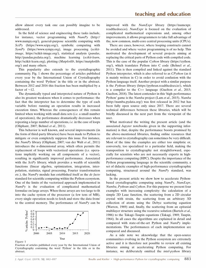
This popularity also extends to the crystallographic

community. Fig. 1 shows the percentage of articles published

every year by the International Union of Crystallography

containing the word ‘Python’ in the title or in the abstract.

Between 2012 and 2016 this fraction has been multiplied by a

factor of �12.

The dynamically typed and interpreted nature of Python is

also its greatest weakness when it comes to performance: the

fact that the interpreter has to determine the type of each

variable before running an operation results in increased

execution times. Whereas the consequences of this remain

limited when working with small data sets (i.e. a small number

of operations), the performance dramatically decreases when

repeating a large number of operations, i.e. in the case of loops

(Oliphant, 2007; Behnel et al., 2011).

This behavior is well known, and several improvements (in

the form of third-party libraries) have been made to Python to

mitigate or even completely suppress this issue. For instance,

the NumPy library (Oliphant, 2007; van der Walt et al., 2011)

introduces the n-dimensional array, which often permits the

replacement of loops with vectorized operations (i.e. opera-

tions implicitly working on all components of a vector),

resulting in significantly improved performance. Associated

with the SciPy library, which provides a wealth of scientific

functions (linear algebra, optimization, integration, inter-

polation, statistics, signal processing, Fourier transformation

etc.), the NumPy module has established itself as the de facto

standard for scientific computing within the Python ecosystem.

One of the limits of the vectorized approach implemented in

NumPy is the evaluation of complicated mathematical

formulae on large arrays. When those arrays are too large to fit

into the cache system of the processor (a few tens of MB),

every single operation needs to fetch and store the data from/

to the central memory. The performance of NumPy can be

improved with the NumExpr library (https://numexpr.

readthedocs.io). NumExpr is focused on the evaluation of

complicated mathematical expressions and, among other

improvements, it allows programmers to take full advantage of

the, now common, multi-core central processing units (CPUs).

There are cases, however, where looping constructs cannot

be avoided and where vector programming is of no help. This

motivated the development of several projects aiming at

replacing the critical parts of Python code with compiled code.

This is the case of the popular Cython library (https://cython.

org/), which translates Python into C code (Behnel et al.,

2011). This is then compiled and linked against the standard

Python interpreter, which is also referred to as CPython (as it

is mainly written in C) in order to avoid confusion with the

Python language itself. Another project with a similar purpose

is the Pythran library (https://pythran.readthedocs.io/), which

is a compiler to the C++ language (Guelton et al., 2015;

Guelton, 2018). The latest contender in this ‘high-performance

Python’ game is the Numba project (Lam et al., 2015). Numba

(http://numba.pydata.org/) was first released in 2012 but has

been fully open source only since 2017. There are several

technical differences between these libraries, which will be

briefly discussed in the next part from the viewpoint of the

user.

What motivated the writing the present article (and the

associated Jupyter notebooks given in the supporting infor-

mation) is that, despite the performance boosts promised by

the above-mentioned libraries, finding online resources that

are relevant to crystallography can sometimes be very difficult.

Most of the time the examples are either too simplistic or,

conversely, too specialized to a particular field, making the

transposition to crystallography not straightforward, espe-

cially for scientists who are not necessarily experts in high-

performance computing (HPC). Despite the importance of the

Python programming language in the scientific community, a

set of didactic examples of high-performance crystallographic

computing, structured around the NumPy standard, was

lacking.

In the present article we show how to accelerate Python-

based crystallographic computing using NumPy, NumExpr,

Numba, Pythran and Cython. For this purpose we present four

examples with increasing complexity: the calculation of a

simple 2D Laue function, the scattering from a 2D circular

crystal with strain, the scattering from an arbitrary 3D

collection of atoms using the Debye scattering equation

(Warren, 1969) and, finally, the scattering from an epitaxial

multilayer structure using the recursive solution (Bartels et al.,

1986) to the Takagi–Taupin equations (Takagi, 1969; Taupin,

1964). In all cases the algorithms are explained in detail and

compared with state-of-the-art Python and NumPy imple-

mentations. The performances of each implementation are

compared and discussed.

As a side note we aknowledge that the open-source

communities evolving in the Python ecosystem are extremely

active and it is therefore not possible to review all existing

libraries aiming at accelerating Python computing. For

instance, we deliberately omitted the intel-python library


J. Appl. Cryst. (2019). 52, 882–897 Boulle and Kieffer � High-performance Python for crystallographic computing 883

Figure 1Fraction of articles published every year by the International Union ofCrystallography containing the word ‘Python’ in the title or in theabstract.

(https://software.intel.com/en-us/distribution-for-python),

which, as the name suggests, is an implementation of the

NumPy library developed by Intel Corporation and optimized

for Intel architectures. As a consequence, it might not operate

correctly with chips from different providers (e.g. AMD) or

with different architectures (e.g. ARM, which is the leading

architecture for the mobile market and is now targeting the PC

and server markets). Moreover, the performance of intel-

python is tightly linked to the exploitation of the multi-core

architecture, a feature which is explicitly included in all of the

above-mentioned libraries. We also omitted the PyPy project

(https://pypy.org/), which is a general-purpose interpreter,

written in Python, aiming at replacing CPython and targeting

high performance. However, with the examples presented in

this article, we did not observe any performance improvement.

2. Computational details

Broadly speaking, performance bottlenecks may originate

either from the power of the CPU, i.e. the number of

instructions it is able to execute over a given time period, or

from data (memory) input/output (Alted, 2010). The former

issue fueled the race to the maximum CPU clock speed (now

capped at around 4 GHz) and the subsequent development of

multi-core CPU architectures. The latter led to what is known

as the hierarchical memory model: since the random-access

memory (RAM) effectively operates at a much lower rate

than the CPU, processor manufacturers introduced on-chip,

smaller but faster, cache memory. Modern CPUs now have up

to three levels of memory cache (L1, L2, L3) with progres-

sively increasing size and decreasing speed. Below we present

the hardware as well the computing libraries used in this work.

Their functioning will be briefly discussed in terms of these

two concepts.

2.1. Library specifications1

In this work, version 1.13.3 of the NumPy library is used. As

mentioned earlier, NumPy introduces the multi-dimensional

array object which, contrarily to the native Python ‘list’ object

(which stores other Python objects), is of fixed size at creation

and contiguously stores data of the same type and size.

Vectorized operations are performed on all elements of an

array, without the necessity to loop over the array coordinates

from the Python code. As a consequence, as illustrated below,

the code is cleaner and closer to mathematical notation. These

vectorized operations are implemented in C, which results in

significant speed improvements (Oliphant, 2007; van der Walt

et al., 2011). The fact that the data are stored contiguously in

the RAM enables one to take advantage of vectorized

instructions of modern CPUs such as SSE (streaming SIMD

extensions, with SIMD meaning ‘single instruction multiple

data’) or AVX (advanced vector extensions), which allows

processing on several data elements per CPU clock cycle

(Rossant, 2018). For instance the AVX2 standard is char-

acterized by 256 bit-wide registers, hence containing four

double-precision (64 bit) floating-point numbers.

NumPy operates optimally when the calculations are

performed on data fitting the cache of the CPU (say, a few tens

of MB). For larger data sets, the performance is limited by the

bandwidth to access the data stored in the RAM. NumExpr

(version 2.6.4 in this work) has been specifically developed to

address these issues with NumPy. NumExpr is a ‘just-in-time’

(JIT) compiler2 for mathematical formulae (relying on an

integrated computing virtual machine), which splits the data

into smaller chunks that fit within the L1 cache of the

processor (a technique known as ‘blocking’) and avoids allo-

cating memory for intermediate results for optimal cache

utilization and reduced memory access. The chunks are

seamlessly distributed among the available cores of the CPU,

which results in highly parallelized code execution.

One important factor limiting Python’s performance is the

conversion from the Python object (‘PyObject’3) to a native

data type. Although NumPy and NumExpr allow this limita-

tion to be lifted by working with arrays with fixed data types,

conversions back and forth from PyObjects to native data

types are still required, which becomes critical when loops or

branching are not avoidable.

The Numba library (version 0.34.0) is a JIT compiler for

Python. Numba relies on LLVM (low level virtual machine,

https://llvm.org/) to produce machine code from Python’s

bytecode that runs at speeds very close to compiled C (Lam et

al., 2015). One of the greatest appeals of Numba is that this

increase in performance is reached with very little code

modification with respect to pure Python code. Moreover,

Numba is compatible with NumPy arrays, supports SIMD

vectorized operations and allows for a straightforward paral-

lelization of loops.

Pythran (version 0.9.0) is an ahead-of-time (AOT) compiler

for Python, which also aims at accelerating scientific compu-

tations; it is therefore also fully compatible with NumPy and

parallel execution (via the openMP project, https://www.

openmp.org/). Pythran not only relies on static typing of

variables but also performs various compiler optimizations to

produce C++ code which is then compiled into native code

(Guelton et al., 2015; Guelton, 2018). Although there are

major technical differences between Numba and Pythran,

from the point of view of the user, their implementation is

quite similar (except for the fact that Pythran requires a

separate compilation step).

The most well known compiler for Python is Cython (here

used in version 0.26.1). Cython produces statically typed C

code which is then executed by the CPython interpreter

(Behnel et al., 2011). Contrarily to Pythran and Numba, which

are domain specific (i.e. scientific) languages, Cython is a

general-purpose AOT compiler. As such, its syntax is more

complex and, contrarily to Numba and Pythran code,


884 Boulle and Kieffer � High-performance Python for crystallographic computing J. Appl. Cryst. (2019). 52, 882–897

1 Different versions of these libraries can produce slightly different timings,but this should not change the conclusions.

2 A JIT compiler compiles the code when it is first called, contrary to ahead-of-time compilers which require a separate compilation step.3 Any Python object (variable, list, dictionary, class etc.) is implement as aPyObject in C. It contains the object type and the references to this object byother objects.

(uncompiled) Cython code is not compatible with the CPython

interpreter. However, this library potentially allows for the

highest level of code optimization.

2.2. Hardware and operating system

All computations were performed on a Linux workstation

equipped with two Intel Xeon E5-2698v4 processors (2 � 20

cores, operating at 2.2 GHz base frequency and 3.6 GHz

maximum frequency) and 194 GB of RAM. The operating

system is Kubuntu 18.04 with version 3.6.6 of the Python

programming language. The Python language and all third-

party libraries were installed from the official software repo-

sitory of the Linux OS used in this work [except Pythran,

which has been installed from the Python package index using

the package installer pip (https://pypi.org/project/pip/)].

Windows and MacOS users might want to use the Anaconda

Python distribution (https://www.anaconda.com/), which

allows for simple module management similar to what is found

in the Linux ecosystem.

Note that, in the context of this article, we are not going to

consider HPC based on graphics processing units (GPUs). The

main reason is that programming such devices requires

specific (computer-scientist) skills which are out of the scope

of this article. Although high-level Python wrappers have been

developed for the two main GPU computing frameworks

(CUDA and OpenCL), getting the best possible performance

out of a given device in general requires the development of

low-level kernels adapted to the device. The second reason is

that, compared with multi-core CPUs, GPUs able to perform

HPC are much less widespread and are in general only to be

found in desktop workstations (i.e. most laptops are

excluded).

3. Implementation

3.1. Two-dimensional Laue function

In this section we are going to present in detail the different

implementations of a given problem using the different

libraries discussed above. For this purpose we shall use a

simple example, namely a two-dimensional Laue function

(Warren, 1969):

IðH;KÞ ¼PN�1

n¼0

PN�1

m¼0

exp 2i�ðHnþ KmÞ½ �

��

2

: ð1Þ

This equation describes the scattering from a square crystal

having N unit cells in both directions; n and m are the indices

of the unit cell in each direction and H and K are the

continuous Miller indices.

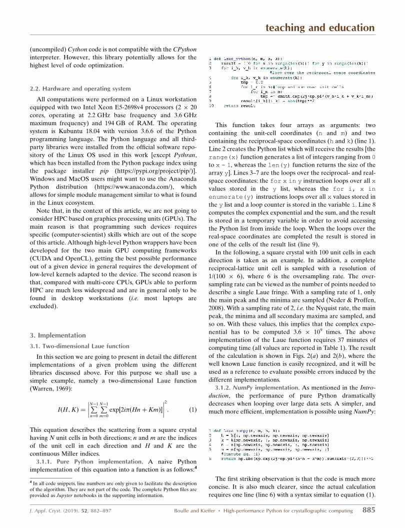
3.1.1. Pure Python implementation. A naive Python

implementation of this equation into a function is as follows:4

This function takes four arrays as arguments: two

containing the unit-cell coordinates (n and m) and two

containing the reciprocal-space coordinates (h and k) (line 1).

Line 2 creates the Python list which will receive the results [the

range(x) function generates a list of integers ranging from 0

to x - 1, whereas the len(y) function returns the size of the

array y]. Lines 3–7 are the loops over the reciprocal- and real-

space coordinates: the for x in y instruction loops over all x

values stored in the y list, whereas the for i, x in

enumerate(y) instructions loops over all x values stored in

the y list and a loop counter is stored in the variable i. Line 8

computes the complex exponential and the sum, and the result

is stored in a temporary variable in order to avoid accessing

the Python list from inside the loop. When the loops over the

real-space coordinates are completed the result is stored in

one of the cells of the result list (line 9).

In the following, a square crystal with 100 unit cells in each

direction is taken as an example. In addition, a complete

reciprocal-lattice unit cell is sampled with a resolution of

1/(100 � 6), where 6 is the oversampling rate. The over-

sampling rate can be viewed as the number of points needed to

describe a single Laue fringe. With a sampling rate of 1, only

the main peak and the minima are sampled (Neder & Proffen,

2008). With a sampling rate of 2, i.e. the Nyquist rate, the main

peak, the minima and all secondary maxima are sampled, and

so on. With these values, this implies that the complex expo-

nential has to be computed 3.6 � 109 times. The above

implementation of the Laue function requires 37 minutes of

computing time (all values are reported in Table 1). The result

of the calculation is shown in Figs. 2(a) and 2(b), where the

well known Laue function is easily recognized, and it will be

used as a reference to evaluate possible errors induced by the

different implementations.

3.1.2. NumPy implementation. As mentioned in the Intro-

duction, the performance of pure Python dramatically

decreases when looping over large data sets. A simpler, and

much more efficient, implementation is possible using NumPy:

The first striking observation is that the code is much more

concise. It is also much clearer, since the actual calculation

requires one line (line 6) with a syntax similar to equation (1).



4 In all code snippets, line numbers are only given to facilitate the descriptionof the algorithm. They are not part of the code. The complete Python files areprovided as Jupyter notebooks in the supporting information.

Lines 2–5 add new (empty) dimensions to the input arrays.

With this transformation the calculation of h*n + k*m actually

returns a four-dimensional array. This important feature of

NumPy is known as ‘broadcasting’. In mathematical notation

this is equivalent to eijkl = aibj + ckdl. The exponential then

operates on all cells of this array, and the sum over the real-

space coordinates is performed using the sum() method of

the NumPy arrays (line 6) [the axis = (2,3)

argument specifies that the summation has to be

performed over the last two dimensions of the

array which contain the real-space variables].

Besides the cleaner syntax, this implementation is

also much faster, with an execution time of

�4 min. Since NumPy is the established standard

for scientific computing, all computing times will

be compared with this NumPy implementation.

3.1.3. NumExpr implementation. The implicit

trade-off that has been made with the NumPy

implementation is that, since the arrays are all

stored in RAM at creation, this operation

requires up to �107 GB of RAM; the four-

dimensional array of complex numbers (coded

over 128 bits) requires 53.6 GB, but twice this

space is needed to compute the exponential. This

issue regarding memory usage is clearly a

limitation of NumPy when dealing with very large

arrays. This could be avoided by creating only one

2D output array and looping over the real-space coordinates

(see ‘NumPy + for loop’ in the supporting information).

However, a more efficient implementation is to use NumExpr,

which, as explained above, makes a better use of memory

allocation and avoids memory transfers. A very interesting

feature of NumExpr is that the code is very similar to that for

NumPy:

There are two differences compared with NumPy. Firstly,

the expression to be evaluated is passed as an argument to a

ne.evaluate() function (lines 8–9). Secondly, the sum

function of NumExpr does not operate over several dimen-

sions (line 9). Therefore the 4D array has been reshaped into a

3D array, where the last dimension contains the real-space

variables (line 8).

When only one thread is used, the acceleration is rather

modest (�1.19). The real power of NumExpr is revealed when

all cores are used (line 7). In the present case, the computing

times drops to 17 s (instead of 4 min for NumPy), that is a

�13.9 speed-up with almost no code modification.

3.1.4. Numba implementation. As mentioned earlier, there

are cases where the mathematical problem cannot be

solved using vector operations (an example will be given in the

last section). In such cases, it can be useful to consider

replacing the critical parts of the program with compiled,

statically typed, code. Below is such an implementation using

Numba:



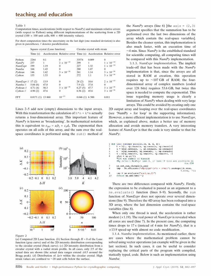
Figure 2(a) Computed 2D Laue function. (b) Section through H = 0 of the Lauefunction (gray curve) and of the 2D intensity distribution correspondingto the circular crystal (black curve). (c) 2D intensity distribution from acircular crystal with a radial strain profile. In all cases, only 2/5 of theactual data are shown (the actual data ranges extend �0.5 around theBragg peak). (d) Distribution of �r/r within the circular crystal. Highstrain values are confined to �20 unit cells below the surface.

Table 1Computation times, accelerations (with respect to NumPy) and maximum relative errors(with respect to Python) using different implementations of the scattering from a 2Dcrystal (100 � 100 unit cells, 600 � 600 intensity values).

For short computation times the uncertainty on the last digit (one standard deviation) is alsogiven in parentheses. // denotes parallelization.

Square crystal (Laue function) Circular crystal with strain

Time (s) Acceleration Relative error Time (s) Acceleration Relative error

Python 2264 0.1 0 33574 0.009 0NumPy 237 1 2 � 10�14 299 1 1 � 10�14

NumExpr 199 1.19 0 227 1.32 1 � 10�14

Numba 166 1.43 0 280 1.07 0Pythran 146 1.62 3 � 10�16 261 1.14 3 � 10�16

Cython 155 1.53 0 272 1.1 3 � 10�16

NumExpr // 17 (2) 13.9 0 28 (2) 10.6 2 � 10�15

Numba // 5.04 (6) 47.0 0 7.9 (2) 37.8 0Pythran // 4.71 (4) 50.3 3 � 10�16 6.27 (5) 47.7 3 � 10�16

Cython // 4.98 (2) 47.6 0 6.56 (2) 45.6 3 � 10�16

FFT 0.0171 (1) 13 860 10�13 0.046 (1) 6 500 0.011

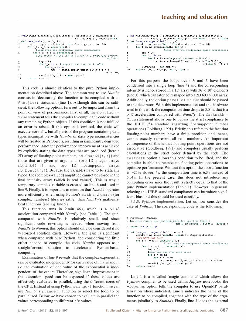
This code is almost identical to the pure Python imple-

mentation described above. The common way to use Numba

consists in ‘decorating’ the function to be compiled with an

@nb.jit() statement (line 1). Although this can be suffi-

cient, the following options turn out to be important from the

point of view of performance. First of all, the nopython =

True statement tells the compiler to compile the code without

any remaining Python objects. If this condition is not fulfilled

an error is raised. If this option is omitted, the code will

execute normally, but all parts of the program containing data

types incompatible with Numba or data-type inconsistencies

will be treated as PyObjects, resulting in significantly degraded

performance. Another performance improvement is achieved

by explicitly stating the data types that are produced (here a

2D array of floating-point numbers, nb.float64[:,:]) and

those that are given as arguments (two 1D integer arrays,

nb.int64[:], and two 1D floating-point arrays,

nb.float64[:]). Because the variables have to be statically

typed, the (complex-valued) amplitude cannot be stored in the

final intensity array (which is real valued). This is why a

temporary complex variable is created on line 6 and used in

line 9. Finally, it is important to mention that Numba operates

more efficiently when using Python’s math and cmath (for

complex numbers) libraries rather than NumPy’s mathema-

tical functions (see e.g. line 9).

This function runs in 2 min 46 s, which is a �1.43

acceleration compared with NumPy (see Table 1). The gain,

compared with NumPy, is relatively small, and since

significant code rewriting is needed when moving from

NumPy to Numba, this option should only be considered if no

vectorized solution exists. However, the gain is significant

when compared with pure Python, and considering the little

effort needed to compile the code, Numba appears as a

straightforward solution to accelerated Python-based

computing.

Examination of line 9 reveals that the complex exponential

can be evaluated independently for each value of h, k, m and n,

i.e. the evaluation of one value of the exponential is inde-

pendent of the others. Therefore, significant improvement in

the execution speed can be expected if these values are

effectively evaluated in parallel, using the different cores of

the CPU. Instead of using Python’s range() function, we can

use Numba’s prange() function to select the loop to be

parallelized. Below we have chosen to evaluate in parallel the

values corresponding to different h/k values:

For this purpose the loops overs h and k have been

condensed into a single loop (line 4) and the corresponding

intensity is hence stored in a 1D array with 36 � 104 elements

(line 3), which can later be reshaped into a 2D 600� 600 array.

Additionally, the option parallel = True should be passed

to the decorator. With this implementation and the hardware

used in this work the computation time drops to 5.04 s, that is a

�47 acceleration compared with NumPy. The fastmath =

True statement allows one to bypass the strict compliance to

the IEEE 754 standard regarding floating-point number

operations (Goldberg, 1991). Briefly, this refers to the fact that

floating-point numbers have a finite precision and, hence,

cannot exactly represent all real numbers. An important

consequence of this is that floating-point operations are not

associative (Goldberg, 1991) and compilers usually perform

calculations in the strict order defined by the code. The

fastmath option allows this condition to be lifted, and the

compiler is able to reassociate floating-point operations to

optimize performance. Without this option the above function

is �25% slower, i.e. the computation time is 6.3 s instead of

5.04 s. In the present case, this does not introduce any

computing error since the result is strictly equal to that of the

pure Python implementation (Table 1). However, in general,

relaxing the IEEE standard compliance can introduce signif-

icant bias and this should be used carefully.

3.1.5. Pythran implementation. Let us now consider the

case of Pythran. The corresponding code is the following:

Line 1 is a so-called ‘magic command’ which allows the

Pythran compiler to be used within Jupyter notebooks; the

-fopenmp option tells the compiler to use OpenMP paral-

lelization where indicated. Line 2 indicates the name of the

function to be compiled, together with the type of the argu-

ments (similarly to Numba). Finally, line 3 loads the external



libraries needed to build the compiled code. The rest of the

code is identical to pure Python or Numba. The performance

is slightly better than that of Numba, with an execution time of

4.7 s, i.e. a �50 acceleration compared with NumPy. Similarly

to what is observed for Numba, the performance boost prin-

cipally originates from the parallelization (when the code runs

on a single thread, the speed-up is �1.62).

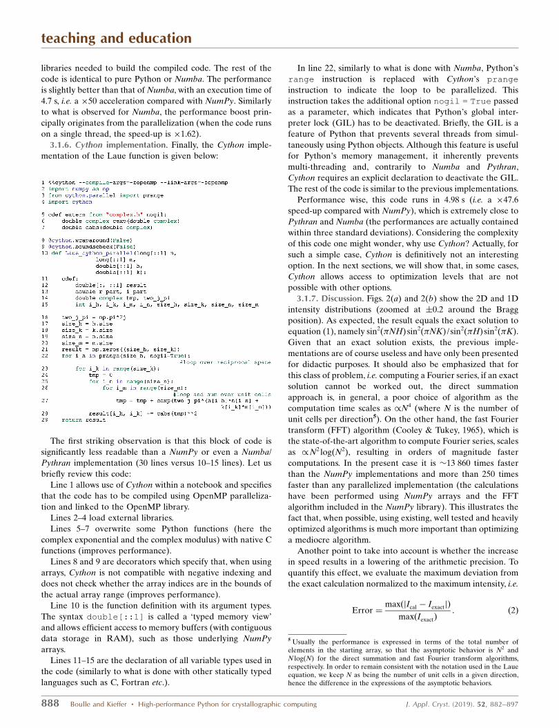
3.1.6. Cython implementation. Finally, the Cython imple-

mentation of the Laue function is given below:

The first striking observation is that this block of code is

significantly less readable than a NumPy or even a Numba/

Pythran implementation (30 lines versus 10–15 lines). Let us

briefly review this code:

Line 1 allows use of Cython within a notebook and specifies

that the code has to be compiled using OpenMP paralleliza-

tion and linked to the OpenMP library.

Lines 2–4 load external libraries.

Lines 5–7 overwrite some Python functions (here the

complex exponential and the complex modulus) with native C

functions (improves performance).

Lines 8 and 9 are decorators which specify that, when using

arrays, Cython is not compatible with negative indexing and

does not check whether the array indices are in the bounds of

the actual array range (improves performance).

Line 10 is the function definition with its argument types.

The syntax double[::1] is called a ‘typed memory view’

and allows efficient access to memory buffers (with contiguous

data storage in RAM), such as those underlying NumPy

arrays.

Lines 11–15 are the declaration of all variable types used in

the code (similarly to what is done with other statically typed

languages such as C, Fortran etc.).

In line 22, similarly to what is done with Numba, Python’s

range instruction is replaced with Cython’s prange

instruction to indicate the loop to be parallelized. This

instruction takes the additional option nogil = True passed

as a parameter, which indicates that Python’s global inter-

preter lock (GIL) has to be deactivated. Briefly, the GIL is a

feature of Python that prevents several threads from simul-

taneously using Python objects. Although this feature is useful

for Python’s memory management, it inherently prevents

multi-threading and, contrarily to Numba and Pythran,

Cython requires an explicit declaration to deactivate the GIL.

The rest of the code is similar to the previous implementations.

Performance wise, this code runs in 4.98 s (i.e. a �47.6

speed-up compared with NumPy), which is extremely close to

Pythran and Numba (the performances are actually contained

within three standard deviations). Considering the complexity

of this code one might wonder, why use Cython? Actually, for

such a simple case, Cython is definitively not an interesting

option. In the next sections, we will show that, in some cases,

Cython allows access to optimization levels that are not

possible with other options.

3.1.7. Discussion. Figs. 2(a) and 2(b) show the 2D and 1D

intensity distributions (zoomed at �0.2 around the Bragg

position). As expected, the result equals the exact solution to

equation (1), namely sin2(�NH)sin2(�NK) / sin2(�H)sin2(�K).

Given that an exact solution exists, the previous imple-

mentations are of course useless and have only been presented

for didactic purposes. It should also be emphasized that for

this class of problem, i.e. computing a Fourier series, if an exact

solution cannot be worked out, the direct summation

approach is, in general, a poor choice of algorithm as the

computation time scales as /N4 (where N is the number of

unit cells per direction5). On the other hand, the fast Fourier

transform (FFT) algorithm (Cooley & Tukey, 1965), which is

the state-of-the-art algorithm to compute Fourier series, scales

as /N2 log(N2), resulting in orders of magnitude faster

computations. In the present case it is �13 860 times faster

than the NumPy implementations and more than 250 times

faster than any parallelized implementation (the calculations

have been performed using NumPy arrays and the FFT

algorithm included in the NumPy library). This illustrates the

fact that, when possible, using existing, well tested and heavily

optimized algorithms is much more important than optimizing

a mediocre algorithm.

Another point to take into account is whether the increase

in speed results in a lowering of the arithmetic precision. To

quantify this effect, we evaluate the maximum deviation from

the exact calculation normalized to the maximum intensity, i.e.

Error ¼maxðjIcal � IexactjÞ

maxðIexactÞ: ð2Þ



5 Usually the performance is expressed in terms of the total number ofelements in the starting array, so that the asymptotic behavior is N2 andN log(N) for the direct summation and fast Fourier transform algorithms,respectively. In order to remain consistent with the notation used in the Laueequation, we keep N as being the number of unit cells in a given direction,hence the difference in the expressions of the asymptotic behaviors.

The results are given in Table 1. All errors are below one

part in 1013, which is several orders of magnitude lower than

the dynamic range that can be experimentally achieved on

diffractometers, even at synchrotron facilities (�108–1010).

Moreover as soon as lattice disorder is present, the experi-

mental dynamic range rapidly decreases (Favre-Nicolin et al.,

2011) so that the present implementations can be used safely

without worrying about the numerical precision.

To conclude this first part, it is worth mentioning that the

results presented here should in no way be taken as general.

The performance of a given library depends on many external

parameters (i.e. it does not solely depend on the imple-

mentation of the algorithm). For example, the size of the

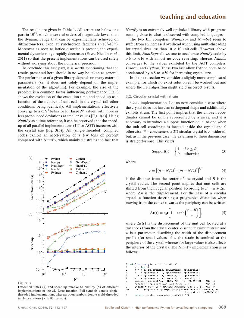
problem is a common factor influencing performance. Fig. 3

shows the evolution of the execution time and speed-up as a

function of the number of unit cells in the crystal (all other

conditions being identical). All implementations effectively

converge to a /N4 behavior for large N2 values, with more or

less pronounced deviations at smaller values [Fig. 3(a)]. Using

NumPy as a time reference, it can be observed that the speed-

up of all parallel implementations (JIT or AOT) increases with

the crystal size [Fig. 3(b)]. All (single-threaded) compiled

codes exhibit an acceleration of a few tens of percent

compared with NumPy, which mainly illustrates the fact that

NumPy is an extremely well optimized library with programs

running close to what is observed with compiled languages.

The two JIT compilers (NumExpr and Numba) seem to

suffer from an increased overhead when using multi-threading

for crystal sizes less than 10 � 10 unit cells. However, above

this limit, NumExpr allows one to accelerate NumPy code by

�6 to �16 with almost no code rewriting, whereas Numba

converges to the values exhibited by the AOT compilers,

Pythran and Cython. These two last allow Python code to be

accelerated by �8 to �50 for increasing crystal size.

In the next section we consider a slightly more complicated

example, for which no exact solution can be worked out and

where the FFT algorithm might yield incorrect results.

3.2. Circular crystal with strain

3.2.1. Implementation. Let us now consider a case where

the crystal does not have an orthogonal shape and additionally

exhibits strain. The first point implies that the unit-cell coor-

dinates cannot be simply represented by a array, and it is

necessary to introduce a support function equal to one when

the unit-cell coordinate is located inside the crystal and 0

otherwise. For conciseness, a 2D circular crystal is considered,

but, as in the previous case, the extension to three dimensions

is straightforward. This yields

SupportðrÞ ¼1 if r � R;0 otherwise

�ð3Þ

where

r ¼ n� N=2ð Þ2þ m� N=2ð Þ

2� �1=2

ð4Þ

is the distance from the center of the crystal and R is the

crystal radius. The second point implies that unit cells are

shifted from their regular position according to n0 = n + �n,

where �n is the displacement. For the case of a circular

crystal, a function describing a progressive dilatation when

moving from the center towards the periphery can be written:

�rðrÞ ¼ e0r 1� tanhr� R

w

� �� ; ð5Þ

where �r(r) is the displacement of the unit cell located at a

distance r from the crystal center, e0 is the maximum strain and

w is a parameter describing the width of the displacement

profile (for small values of w the strain is confined at the

periphery of the crystal, whereas for large values it also affects

the interior of the crystal). The NumPy implementation is as

follows:



Figure 3Execution times (a) and speed-up relative to NumPy (b) of differentimplementations of the 2D Laue function. Full symbols denote single-threaded implementations, whereas open symbols denote multi-threadedimplementations (with 80 threads).

The radius from the center of the unit cell is computed in

line 7 and it is a 2D array (with two additional empty

dimensions). The support function is computed in line 8 and

sets to 0 all values for which the radius is larger than the crystal

radius (here chosen as R = N/2). The strain �r/r is computed in

line 9 and, similarly to the radius and the support function, it is

a 2D array with two additional empty dimensions dedicated to

receiving the reciprocal-space coordinates (line 10). Strictly

speaking, it is not necessary to explicitly define the support

function (line 8), in the sense that we could limit the evalua-

tion of the tmp variable only to those regions where the

condition radius < N/2 is fulfilled. Thereby we would save the

corresponding memory space (although without improvement

regarding the execution speed). We nonetheless keep this

implementation here for didactic purposes; the modified

version is implemented in the following versions below.

Afterwards, similarly to the Laue function, the summation

over the unit-cell coordinates is performed using the sum

method of NumPy. As observed in the previous section, the

broadcasting and vectorizing properties of NumPy allow for a

painless implementation of mathematical equations.

Fig. 2(b) shows a section along the K direction (performed

at H = 0 and around K = 4) with e0 = 0.01 and w = 20, and

Fig. 2(c) shows a portion of the 2D intensity distribution.

Fig. 2(d) shows the distribution of �r/r within the crystal

computed with equation (3). The crystal is tensily strained, so

that the peak is shifted towards lower K values and, since the

distribution of strain is inhomogeneous, the intensity distri-

bution is broadened and asymmetric compared with the Laue

function.

This implementation runs in �299 s, which is more than 100

times faster than the pure Python implementation (given in

the corresponding notebook). In this case, the acceleration is

more than 10 times greater than in the previous section, i.e. the

Python implementation required more than 9 h instead of

37 min for the Laue function, whereas the NumPy imple-

mentation only required�62 s more (299 versus 237 s). This is

because the relative efficiency of NumPy increases when the

number of floating-point operations within the loops increases.

The NumExpr implementation is similar to the NumPy

code and only differs by calls to the ne.evaluate() func-

tion:

Notice that in this implementation we did not explicitly

define the support function and we merged its definition with

the evaluation of the complex exponential (line 11). Among

all (single-threaded) implementations, NumExpr exhibits the

best performance with �1.32 speed-up, whereas the worst

result is obtained with Numba with a �1.07 speed-up

compared with NumPy (see Table 1). As mentioned in the

previous section, this again illustrates the efficiency of the

NumPy library. In the rest of the article we shall therefore

focus on the results obtained with the parallel versions of the

algorithms, since this is when the best performance is

obtained.

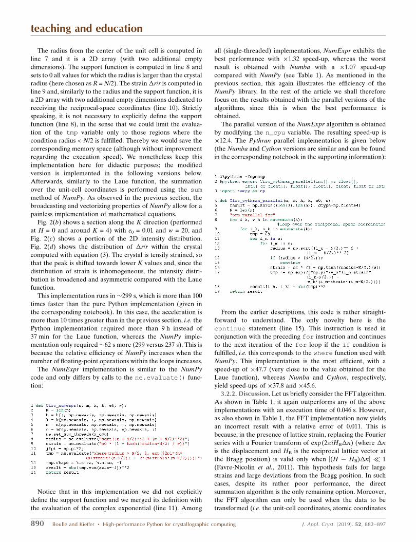
The parallel version of the NumExpr algorithm is obtained

by modifying the n_cpu variable. The resulting speed-up is

�12.4. The Pythran parallel implementation is given below

(the Numba and Cython versions are similar and can be found

in the corresponding notebook in the supporting information):

From the earlier descriptions, this code is rather straight-

forward to understand. The only novelty here is the

continue statement (line 15). This instruction is used in

conjunction with the preceding for instruction and continues

to the next iteration of the for loop if the if condition is

fulfilled, i.e. this corresponds to the where function used with

NumPy. This implementation is the most efficient, with a

speed-up of �47.7 (very close to the value obtained for the

Laue function), whereas Numba and Cython, respectively,

yield speed-ups of �37.8 and �45.6.

3.2.2. Discussion. Let us briefly consider the FFT algorithm.

As shown in Table 1, it again outperforms any of the above

implementations with an execution time of 0.046 s. However,

as also shown in Table 1, the FFT implementation now yields

an incorrect result with a relative error of 0.011. This is

because, in the presence of lattice strain, replacing the Fourier

series with a Fourier transform of exp(2�iHB�n) (where �n

is the displacement and HB is the reciprocal lattice vector at

the Bragg position) is valid only when |(H � HB)�n| 1

(Favre-Nicolin et al., 2011). This hypothesis fails for large

strains and large deviations from the Bragg position. In such

cases, despite its rather poor performance, the direct

summation algorithm is the only remaining option. Moreover,

the FFT algorithm can only be used when the data to be

transformed (i.e. the unit-cell coordinates, atomic coordinates



etc.) can be represented on a regular grid, like a 3D array of (x,

y, z) coordinates. This constraint therefore excludes atomistic

simulation results, for which the direct summation algorithm is

thus the only remaining option to compute the diffracted

intensity. The possibility to accelerate such computations can

hence be relevant in such situations.

As mentioned in Section 2, in this work we are not

considering the implementation on GPUs. However, it is

worth mentioning the existence of a Python library called

PyNX (Favre-Nicolin et al., 2011), specifically developed

(among other tasks) to optimize the direct summation algo-

rithm of the Fourier transform (http://ftp.esrf.fr/pub/scisoft/

PyNX/doc/). Given its highly parallel nature, PyNX strongly

benefits from the architecture of GPUs and yields far better

results than the present implementations.

3.3. The Debye scattering equation

For didactic purposes, the two previous sections were

focused on theoretical 2D crystals. We now consider a slightly

more complex example, namely the scattering from actual

nanocrystals. Assuming that the crystals exhibit all possible

orientations (like in a powder sample), the intensity scattered

by an ensemble of N atoms is correctly described by the Debye

scattering equation (Warren, 1969):

IðQÞ ¼XN

i¼1

XN

j¼1

fiðQÞ fjðQÞsinðQrijÞ

Qrij

; ð6Þ

where Q = 4�sin(�)/� (� being half the scattering angle and �the radiation wavelength), fi is the atomic scattering factor of

the ith atom and rij are the distances between all possible pairs

of atoms in the crystal. For the sake of simplicity we shall

consider a mono-atomic crystal. In such a case, the scattering

equation can be simplified to

IðQÞ ¼ j f ðQÞj2 N þ 2XN

i¼1

XN

j> i

sinðQrijÞ

Qrij

" #: ð7Þ

The extension to polyatomic crystals is straightforwardly

obtained by computing equation (7) for all possible homo-

atomic and hetero-atomic pairs.

An interesting feature of this equation is that it does not

require the existence of an average crystal lattice so that,

contrarily to the previous section, the intensity can be

computed even from highly disordered crystals, or from

liquids, gasses . . . . From a computational point of view, this

also implies that one can make use of atomic coordinates

obtained by atomic scale calculations (like molecular

dynamics for instance) to compute the corresponding

intensity and compare it with the diffraction pattern from

actual nanostructured materials. The examination of equation

(7) reveals that the calculation actually requires two distinct

steps:

(i) The calculation of all pairwise distances, rij, from a given

collection of (x, y, z) coordinates.

(ii) The calculation of the double sum.

3.3.1. Calculation of the pairwise distances. Computing all

pairwise distances actually consists in computing the Eucli-

dean distance matrix with component rij:

rij ¼ jjri � rjjj; ð8Þ

where || . . . || is the Euclidean norm. All diagonal elements are

zero (rii = 0) and the matrix is symmetrical (rij = rji) so that only

a triangular part needs to be computed. A naive Python

implementation is as follows:

For a collection of N = 4753 atoms (with coordinates stored

in the 2D [N � 3] array coords) this algorithm runs in 24.2 s

(Table 2). As usual, far better results are to be expected with a

NumPy implementation. For instance, developing equation

(8) yields

rij ¼ ðri � rjÞTðri � rjÞ

� �1=2¼ rT

i ri � 2rTi rj � rT

j rj

�1=2: ð9Þ



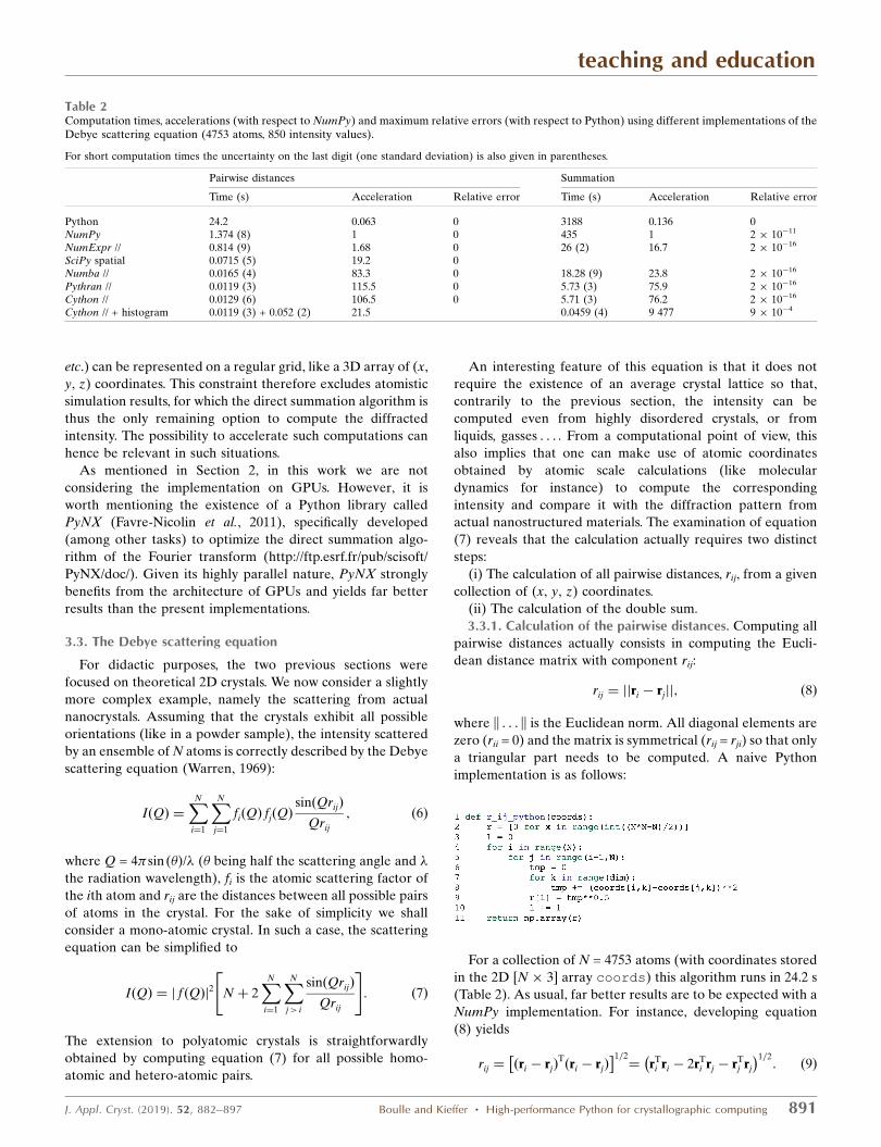
Table 2Computation times, accelerations (with respect to NumPy) and maximum relative errors (with respect to Python) using different implementations of theDebye scattering equation (4753 atoms, 850 intensity values).

For short computation times the uncertainty on the last digit (one standard deviation) is also given in parentheses.

Pairwise distances Summation

Time (s) Acceleration Relative error Time (s) Acceleration Relative error

Python 24.2 0.063 0 3188 0.136 0NumPy 1.374 (8) 1 0 435 1 2 � 10�11

NumExpr // 0.814 (9) 1.68 0 26 (2) 16.7 2 � 10�16

SciPy spatial 0.0715 (5) 19.2 0Numba // 0.0165 (4) 83.3 0 18.28 (9) 23.8 2 � 10�16

Pythran // 0.0119 (3) 115.5 0 5.73 (3) 75.9 2 � 10�16

Cython // 0.0129 (6) 106.5 0 5.71 (3) 76.2 2 � 10�16

Cython // + histogram 0.0119 (3) + 0.052 (2) 21.5 0.0459 (4) 9 477 9 � 10�4

The corresponding NumPy code reads (Bauckhage, 2014)

Line 2 computes the rTi rj dot product; line 3 creates the rT

i ri

matrix by extracting the diagonal of the dot product computed

in line 2 and repeating (tile) it over N columns, and line 4

computes equation (9). Finally, line 5 sets to 0 all elements of

the lower triangular matrix (triu) and only the nonzero

elements are returned. This implementation runs in 1.374 s.

The NumExpr code is quite similar (see notebooks) and

only differs from the previous NumPy implementation in lines

4 and 5 by calls to the ne.evalute() function. The corre-

sponding implementation runs in 814 ms, which is a �1.68

speed-up compared with NumPy.

Before proceeding to the parallelized implementations we

note that the SciPy library has a collection of functions

devoted to analysis of data structures representing spatial

properties (scipy.spatial). Using this library, the Eucli-

dean matrix can be computed in a single line of code:

where pdist is the function that computes all pairwise

distances within the list of coordinates coords. Interestingly

this function runs at the same speed as a compiled imple-

mentation, 71.5 ms (�19.2), which outperforms both NumPy

and NumExpr. This result, again, illustrates the importance of

using third-party libraries that contain efficient and well tested

code rather than reinventing the wheel.

Inspection of the Python implementation reveals that the

algorithm could benefit from further acceleration by paralle-

lizing the first for loops. The Pythran implementation is

shown below:

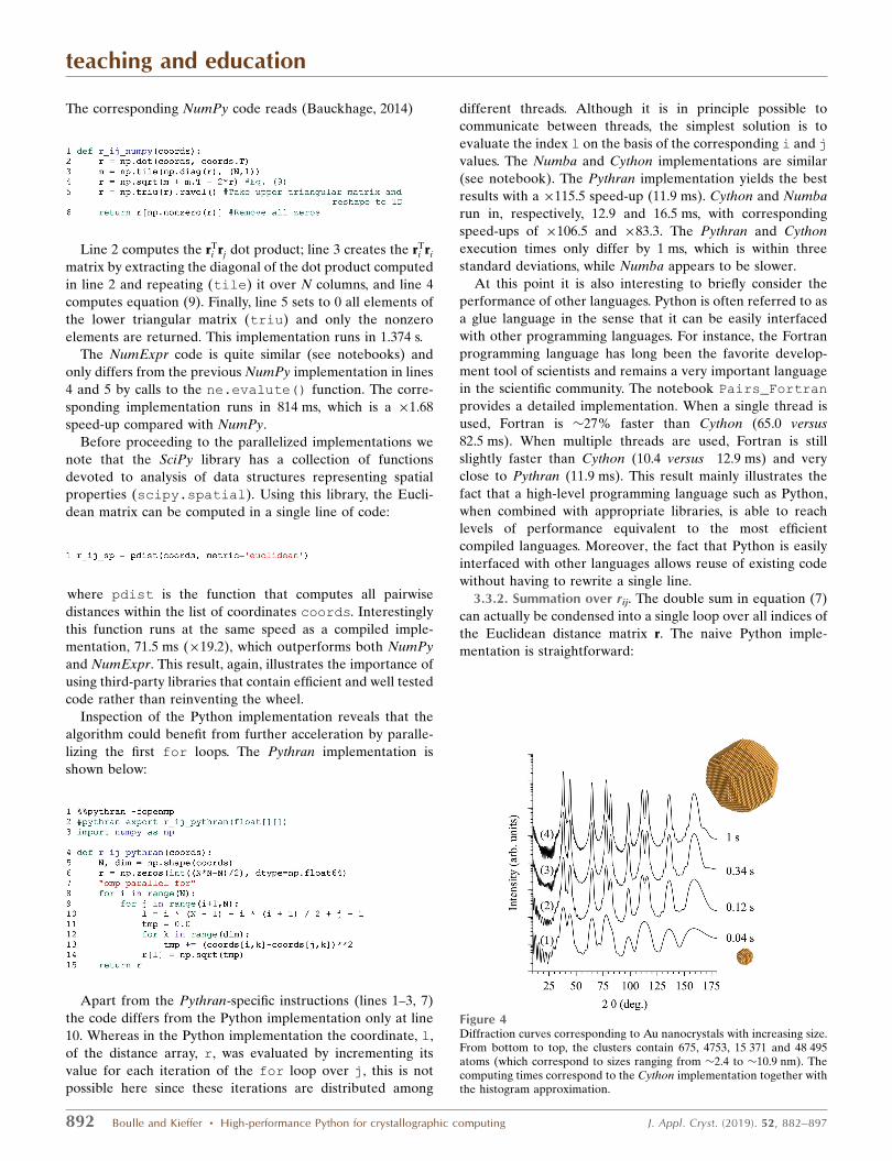
Apart from the Pythran-specific instructions (lines 1–3, 7)

the code differs from the Python implementation only at line

10. Whereas in the Python implementation the coordinate, l,

of the distance array, r, was evaluated by incrementing its

value for each iteration of the for loop over j, this is not

possible here since these iterations are distributed among

different threads. Although it is in principle possible to

communicate between threads, the simplest solution is to

evaluate the index l on the basis of the corresponding i and j

values. The Numba and Cython implementations are similar

(see notebook). The Pythran implementation yields the best

results with a �115.5 speed-up (11.9 ms). Cython and Numba

run in, respectively, 12.9 and 16.5 ms, with corresponding

speed-ups of �106.5 and �83.3. The Pythran and Cython

execution times only differ by 1 ms, which is within three

standard deviations, while Numba appears to be slower.

At this point it is also interesting to briefly consider the

performance of other languages. Python is often referred to as

a glue language in the sense that it can be easily interfaced

with other programming languages. For instance, the Fortran

programming language has long been the favorite develop-

ment tool of scientists and remains a very important language

in the scientific community. The notebook Pairs_Fortran

provides a detailed implementation. When a single thread is

used, Fortran is �27% faster than Cython (65.0 versus

82.5 ms). When multiple threads are used, Fortran is still

slightly faster than Cython (10.4 versus 12.9 ms) and very

close to Pythran (11.9 ms). This result mainly illustrates the

fact that a high-level programming language such as Python,

when combined with appropriate libraries, is able to reach

levels of performance equivalent to the most efficient

compiled languages. Moreover, the fact that Python is easily

interfaced with other languages allows reuse of existing code

without having to rewrite a single line.

3.3.2. Summation over rij. The double sum in equation (7)

can actually be condensed into a single loop over all indices of

the Euclidean distance matrix r. The naive Python imple-

mentation is straightforward:



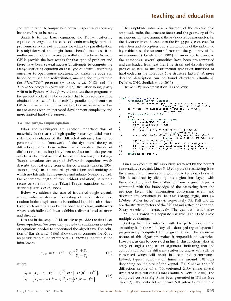
Figure 4Diffraction curves corresponding to Au nanocrystals with increasing size.From bottom to top, the clusters contain 675, 4753, 15 371 and 48 495atoms (which correspond to sizes ranging from �2.4 to �10.9 nm). Thecomputing times correspond to the Cython implementation together withthe histogram approximation.

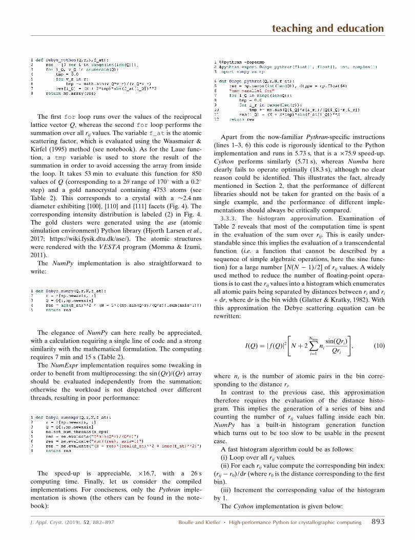
The first for loop runs over the values of the reciprocal

lattice vector Q, whereas the second for loop performs the

summation over all rij values. The variable f_at is the atomic

scattering factor, which is evaluated using the Waasmaier &

Kirfel (1995) method (see notebook). As for the Laue func-

tion, a tmp variable is used to store the result of the

summation in order to avoid accessing the array from inside

the loop. It takes 53 min to evaluate this function for 850

values of Q (corresponding to a 2� range of 170 with a 0.2

step) and a gold nanocrystal containing 4753 atoms (see

Table 2). This corresponds to a crystal with a �2.4 nm

diameter exhibiting {100}, {110} and {111} facets (Fig. 4). The

corresponding intensity distribution is labeled (2) in Fig. 4.

The gold clusters were generated using the ase (atomic

simulation environment) Python library (Hjorth Larsen et al.,

2017; https://wiki.fysik.dtu.dk/ase/). The atomic structures

were rendered with the VESTA program (Momma & Izumi,

2011).

The NumPy implementation is also straightforward to

write:

The elegance of NumPy can here really be appreciated,

with a calculation requiring a single line of code and a strong

similarity with the mathematical formulation. The computing

requires 7 min and 15 s (Table 2).

The NumExpr implementation requires some tweaking in

order to benefit from multiprocessing: the sin(Qr)/(Qr) array

should be evaluated independently from the summation;

otherwise the workload is not dispatched over different

threads, resulting in poor performance:

The speed-up is appreciable, �16.7, with a 26 s

computing time. Finally, let us consider the compiled

implementations. For conciseness, only the Pythran imple-

mentation is shown (the others can be found in the note-

book):

Apart from the now-familiar Pythran-specific instructions

(lines 1–3, 6) this code is rigorously identical to the Python

implementation and runs in 5.73 s, that is a �75.9 speed-up.

Cython performs similarly (5.71 s), whereas Numba here

clearly fails to operate optimally (18.3 s), although no clear

reason could be identified. This illustrates the fact, already

mentioned in Section 2, that the performance of different

libraries should not be taken for granted on the basis of a

single example, and the performance of different imple-

mentations should always be critically compared.

3.3.3. The histogram approximation. Examination of

Table 2 reveals that most of the computation time is spent

in the evaluation of the sum over rij. This is easily under-

standable since this implies the evaluation of a transcendental

function (i.e. a function that cannot be described by a

sequence of simple algebraic operations, here the sine func-

tion) for a large number [N(N � 1) /2] of rij values. A widely

used method to reduce the number of floating-point opera-

tions is to cast the rij values into a histogram which enumerates

all atomic pairs being separated by distances between ri and ri

+ dr, where dr is the bin width (Glatter & Kratky, 1982). With

this approximation the Debye scattering equation can be

rewritten:

IðQÞ ¼ j f ðQÞj2 N þ 2XNbins

i¼1

ni

sinðQriÞ

Qri

" #; ð10Þ

where ni is the number of atomic pairs in the bin corre-

sponding to the distance ri.

In contrast to the previous case, this approximation

therefore requires the evaluation of the distance histo-

gram. This implies the generation of a series of bins and

counting the number of rij values falling inside each bin.

NumPy has a built-in histogram generation function

which turns out to be too slow to be usable in the present

case.

A fast histogram algorithm could be as follows:

(i) Loop over all rij values.

(ii) For each rij value compute the corresponding bin index:

(rij� r0) /dr (where r0 is the distance corresponding to the first

bin).

(iii) Increment the corresponding value of the histogram

by 1.

The Cython implementation is given below:



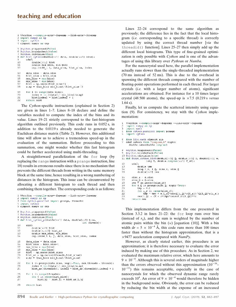
The Cython-specific instructions (explained in Section 2)

are given in lines 1–7. Lines 8–18 declare and define the

variables needed to compute the index of the bins and its

value. Lines 19–21 strictly correspond to the fast-histogram

algorithm outlined previously. This code runs in 0.052 s, in

addition to the 0.0119 s already needed to generate the

Euclidean distance matrix (Table 2). However, this additional

time will allow us to achieve a tremendous speed-up in the

evaluation of the summation. Before proceeding to this

summation, one might wonder whether this fast histogram

could be further accelerated using multi-threading.

A straightforward parallelization of the for loop (by

replacing the range instruction with a prange instruction, line

18) results in erroneous results since there is no mechanism that

prevents the different threads from writing in the same memory

block at the same time, hence resulting in a wrong numbering of

distances in the histogram. This issue can be circumvented by

allocating a different histogram to each thread and then

combining them together. The corresponding code is as follows:

Lines 22–24 correspond to the same algorithm as

previously; the difference lies in the fact that the local histo-

gram (i.e. corresponding to a specific thread) is correctly

updated by using the correct thread number [via the

threadid() function]. Lines 25–27 then simply add up the

different local histograms. This type of fine-grained optimi-

zation is only possible with Cython and is one of the advan-

tages of using this library over Pythran or Numba.

For the nanocrystal used here, the parallel implementation

actually runs slower than the single-threaded implementation

(70 ms instead of 52 ms). This is due to the overhead in

spawning the different threads compared with the number of

floating-point operations performed in each thread. For larger

crystals (i.e. with a larger number of atoms), significant

accelerations are obtained. For instance for a 10 times larger

crystal (48 500 atoms), the speed-up is �7.5 (0.219 s versus

1.64 s).

Finally, let us compute the scattered intensity using equa-

tion (9). For consistency, we stay with the Cython imple-

mentation:

This implementation differs from the one presented in

Section 3.3.2 in lines 21–22: the for loop runs over bins

(instead of rij), and the sum is weighted by the number of

atomic pairs within the bin (w) [equation (10)]. With a bin

width dr = 5 � 10�4 A, this code runs more than 100 times

faster than without the histogram approximation, that is a

�9477 acceleration compared with NumPy.

However, as clearly stated earlier, this procedure is an

approximation; it is therefore necessary to evaluate the error

induced by making use of this procedure. As in Section 2, we

evaluated the maximum relative error, which here amounts to

9 � 10�4. Although this is several orders of magnitude higher

than the errors observed without this approximation (10�16–

10�11) this remains acceptable, especially in the case of

nanocrystals for which the observed dynamic range rarely

exceeds 104. An error of 9 � 10�4 would therefore be hidden

in the background noise. Obviously, the error can be reduced

by reducing the bin width at the expense of an increased



computing time. A compromise between speed and accuracy

has therefore to be made.

Similarly to the Laue equation, the Debye scattering

equation belongs to this class of ‘embarrassingly parallel’

problems, i.e. a class of problems for which the parallelization

is straightforward and might hence benefit the most from

multi-core and other massively parallel architectures. As such,

GPUs provide the best results for that type of problem and

there have been several successful attempts to compute the

Debye scattering equation on that type of device. Restricting

ourselves to open-source solutions, for which the code can

hence be reused and redistributed, one can cite for example

the PHAISTOS program (Antonov et al., 2012) and the

XaNSoNS program (Neverov, 2017), the latter being partly

written in Python. Although we did not test these programs in

the present work, it can be expected that better results will be

obtained because of the massively parallel architecture of

GPUs. However, as outlined earlier, this increase in perfor-

mance comes with an increased development complexity and

more limited hardware support.

3.4. The Takagi–Taupin equation

Films and multilayers are another important class of

materials. In the case of high-quality hetero-epitaxial mate-

rials, the calculation of the diffracted intensity has to be

performed in the framework of the dynamical theory of

diffraction, rather than within the kinematical theory of

diffraction that has implicitly been used so far in the present

article. Within the dynamical theory of diffraction, the Takagi–

Taupin equations are coupled differential equations which

describe the scattering from distorted crystals (Takagi, 1969;

Taupin, 1964). In the case of epitaxial films and multilayers

which are laterally homogeneous and infinite (compared with

the coherence length of the incident radiation), a simple

recursive solution to the Takagi–Taupin equations can be

derived (Bartels et al., 1986).

Below, we address the case of irradiated single crystals

where radiation damage (consisting of lattice strain and

random lattice displacement) is confined in a thin sub-surface

layer. Such materials can be described as arbitrary multilayers

where each individual layer exhibits a distinct level of strain

and disorder.

It is not in the scope of this article to provide the details of

these equations. We here only provide the minimum number

of equations needed to understand the algorithms. The solu-

tion of Bartels et al. (1986) allows one to compute the X-ray

amplitude ratio at the interface n + 1, knowing the ratio at the

interface n:

Xnþ1 ¼ �þ ð�2� 1Þ1=2 S1 þ S2

S1 � S2

; ð11Þ

where

S1 ¼ Xn � �þ ð�2� 1Þ1=2

� �exp �iTð�2

� 1Þ1=2� �

;

S2 ¼ Xn � �� ð�2 � 1Þ1=2

� �exp iTð�2 � 1Þ1=2

� �:

ð12Þ

The amplitude ratio X is a function of the electric field

amplitude ratio, the structure factor and the geometry of the

measurement. � is dynamical theory’s deviation parameter, i.e.

the deviation from the center of the Bragg peak, corrected for

refraction and absorption, and T is a function of the individual

layer thickness, the structure factor and the geometry of the

measurement (Bartels et al., 1986). In order not to overload

the notebooks, several quantities have been pre-computed

and are loaded from text files (the strain and disorder depth

profiles as well as the instrumental resolution function) or

hard-coded in the notebook (the structure factors). A more

detailed description can be found elsewhere (Boulle &

Debelle, 2010; Souilah et al., 2016).

The NumPy implementation is as follows:

Lines 2–3 compute the amplitude scattered by the perfect

(unirradiated) crystal. Lines 5–15 compute the scattering from

the strained and disordered region above the perfect crystal.

This is achieved by dividing this region into layers with

thickness t_l, and the scattering from a given layer is

computed with the knowledge of the scattering from the

previous layer. The information concerning strain and

disorder are contained in the thB (Bragg angle) and DW

(Debye–Waller factor) arrays, respectively. FH, FmH and wl

are the structure factors of the hkl and hkl reflections and the

X-ray wavelength, respectively. The quantity (eta*eta-

1)**0.5 is stored in a separate variable (line 11) to avoid

multiple evaluations.

Starting from the interface with the perfect crystal, the

scattering from the whole ‘crystal + damaged region’ system is

progressively computed for a given angle. The recursive

nature of this algorithm makes it impossible to vectorize.

However, as can be observed in line 1, this function takes an

array of angles (th) as an argument, indicating that the

computation for the different scattering angles can still be

vectorized which will result in acceptable performance.

Indeed, typical computation times are around 0.01–0.1 s

depending on the size of the crystal. Fig. 5 shows the 400

diffraction profile of a (100)-oriented ZrO2 single crystal

irradiated with 300 keV Cs ions (Boulle & Debelle, 2010). The

computed curve in Fig. 5 has been generated in 18.5 ms (see

Table 3). This data set comprises 501 intensity values; the



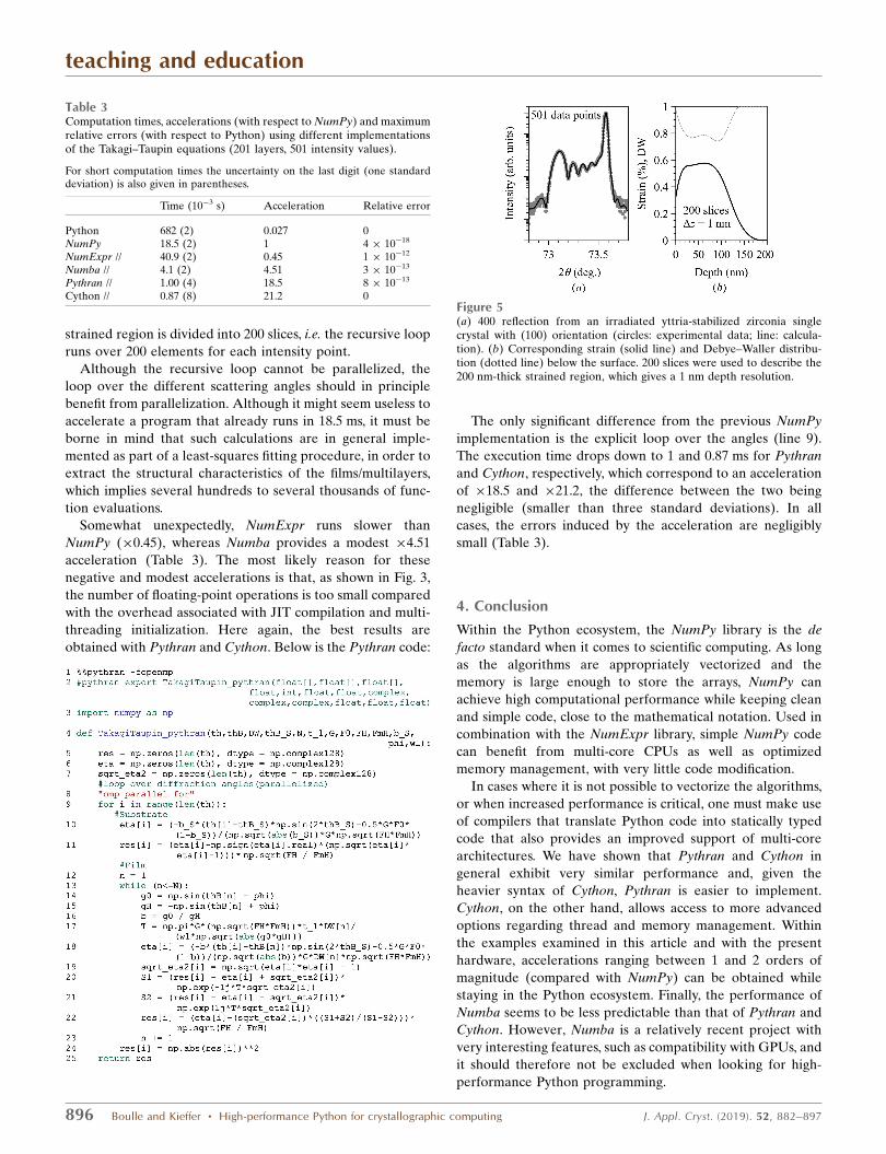
strained region is divided into 200 slices, i.e. the recursive loop

runs over 200 elements for each intensity point.

Although the recursive loop cannot be parallelized, the

loop over the different scattering angles should in principle

benefit from parallelization. Although it might seem useless to

accelerate a program that already runs in 18.5 ms, it must be

borne in mind that such calculations are in general imple-

mented as part of a least-squares fitting procedure, in order to

extract the structural characteristics of the films/multilayers,

which implies several hundreds to several thousands of func-

tion evaluations.

Somewhat unexpectedly, NumExpr runs slower than

NumPy (�0.45), whereas Numba provides a modest �4.51

acceleration (Table 3). The most likely reason for these

negative and modest accelerations is that, as shown in Fig. 3,

the number of floating-point operations is too small compared

with the overhead associated with JIT compilation and multi-

threading initialization. Here again, the best results are

obtained with Pythran and Cython. Below is the Pythran code:

The only significant difference from the previous NumPy

implementation is the explicit loop over the angles (line 9).

The execution time drops down to 1 and 0.87 ms for Pythran

and Cython, respectively, which correspond to an acceleration

of �18.5 and �21.2, the difference between the two being

negligible (smaller than three standard deviations). In all

cases, the errors induced by the acceleration are negligibly

small (Table 3).

4. Conclusion

Within the Python ecosystem, the NumPy library is the de

facto standard when it comes to scientific computing. As long

as the algorithms are appropriately vectorized and the

memory is large enough to store the arrays, NumPy can

achieve high computational performance while keeping clean

and simple code, close to the mathematical notation. Used in

combination with the NumExpr library, simple NumPy code

can benefit from multi-core CPUs as well as optimized

memory management, with very little code modification.

In cases where it is not possible to vectorize the algorithms,

or when increased performance is critical, one must make use

of compilers that translate Python code into statically typed

code that also provides an improved support of multi-core

architectures. We have shown that Pythran and Cython in

general exhibit very similar performance and, given the

heavier syntax of Cython, Pythran is easier to implement.

Cython, on the other hand, allows access to more advanced

options regarding thread and memory management. Within

the examples examined in this article and with the present

hardware, accelerations ranging between 1 and 2 orders of

magnitude (compared with NumPy) can be obtained while

staying in the Python ecosystem. Finally, the performance of

Numba seems to be less predictable than that of Pythran and

Cython. However, Numba is a relatively recent project with

very interesting features, such as compatibility with GPUs, and

it should therefore not be excluded when looking for high-

performance Python programming.



Table 3Computation times, accelerations (with respect to NumPy) and maximumrelative errors (with respect to Python) using different implementationsof the Takagi–Taupin equations (201 layers, 501 intensity values).

For short computation times the uncertainty on the last digit (one standarddeviation) is also given in parentheses.

Time (10�3 s) Acceleration Relative error

Python 682 (2) 0.027 0NumPy 18.5 (2) 1 4 � 10�18

NumExpr // 40.9 (2) 0.45 1 � 10�12

Numba // 4.1 (2) 4.51 3 � 10�13

Pythran // 1.00 (4) 18.5 8 � 10�13

Cython // 0.87 (8) 21.2 0Figure 5(a) 400 reflection from an irradiated yttria-stabilized zirconia singlecrystal with (100) orientation (circles: experimental data; line: calcula-tion). (b) Corresponding strain (solid line) and Debye–Waller distribu-tion (dotted line) below the surface. 200 slices were used to describe the200 nm-thick strained region, which gives a 1 nm depth resolution.

Finally, the ability of Python to interface with other

languages such as C, C++ or Fortran makes it a prominent

language for the development of libraries combining an easy

syntax with the performance of compiled languages. In the

field of crystallography this is for instance the case of the

Computational Crystallography Toolbox project, cctbx

(Grosse-Kunstleve et al., 2002; https://cctbx.github.io/). The

cctbx library is developed as a set of C++ classes that can be

accessed via a Python interface. As such, cctbx can be used in

combination with the libraries presented above. This library is

also a component of several crystallographic software tools.

cctbx is for instance used to compute scattering factors in the

PyNX library mentioned earlier (Favre-Nicolin et al., 2011). In

the field of macromolecular crystallography, it is the key

component of the PHENIX program (Adams et al., 2010;

https://www.phenix-online.org/) which is also written in

Python. Besides cctbx, large-scale facilities are particularly

active in the development of X-ray and neutron scattering

data manipulation and visualization software based on

Python; one can cite DIALS (Winter et al., 2018; https://

dials.github.io/), Mantid (Arnold et al., 2014; https://

www.mantidproject.org/), DAWN (Basham et al., 2015; Filik et

al., 2017; https://dawnsci.org/about/) and silx (https://www.silx.

org/).

Acknowledgements

All figures have been generated with the scientific plotting

program Veusz (https://veusz.github.io/). AB is thankful to D.

Andre for the fruitful discussions about the performance of

various languages.

References

Adams, P. D., Afonine, P. V., Bunkoczi, G., Chen, V. B., Davis, I. W.,Echols, N., Headd, J. J., Hung, L.-W., Kapral, G. J., Grosse-Kunstleve, R. W., McCoy, A. J., Moriarty, N. W., Oeffner, R., Read,R. J., Richardson, D. C., Richardson, J. S., Terwilliger, T. C. &Zwart, P. H. (2010). Acta Cryst. D66, 213–221.

Alted, F. (2010). Comput. Sci. Eng. 12, 68–71.Antonov, L. D., Andreetta, C. & Hamelryck, T. (2012). Proceedings of

the International Conference on Bioinformatics Models, Methodsand Algorithms, pp. 102–108. SciTePress. https://doi.org/10.5220/0003781501020108.

Arnold, O., Bilheux, J. C., Borreguero, J. M., Buts, A., Campbell, S. I.,Chapon, L., Doucet, M., Draper, N., Ferraz Leal, R., Gigg, M. A.,Lynch, V. E., Markvardsen, A., Mikkelson, D. J., Mikkelson, R. L.,Miller, R., Palmen, K., Parker, P., Passos, G., Perring, T. G.,Peterson, P. F., Ren, S., Reuter, M. A., Savici, A. T., Taylor, J. W.,Taylor, R. J., Tolchenov, R., Zhou, W. & Zikovsky, J. (2014). Nucl.Instrum. Methods Phys. Res. A, 764, 156–166.

Bartels, W. J., Hornstra, J. & Lobeek, D. J. W. (1986). Acta Cryst. A42,539–545.

Basham, M., Filik, J., Wharmby, M. T., Chang, P. C. Y., El Kassaby, B.,Gerring, M., Aishima, J., Levik, K., Pulford, B. C. A., Sikharulidze,I., Sneddon, D., Webber, M., Dhesi, S. S., Maccherozzi, F., Svensson,O., Brockhauser, S., Naray, G. & Ashton, A. W. (2015). J.Synchrotron Rad. 22, 853–858.

Bauckhage, C. (2014). Technical Report, https://doi.org/10.13140/2.1.4426.1127.

Behnel, S., Bradshaw, R., Citro, C., Dalcin, L., Seljebotn, D. S. &Smith, K. (2011). Comput. Sci. Eng. 13, 31–39.

Boulle, A. & Debelle, A. (2010). J. Appl. Cryst. 43, 1046–1052.Cooley, J. W. & Tukey, J. W. (1965). Math. Comp. 19, 297–301.Favre-Nicolin, V., Coraux, J., Richard, M.-I. & Renevier, H. (2011). J.

Appl. Cryst. 44, 635–640.Filik, J., Ashton, A. W., Chang, P. C. Y., Chater, P. A., Day, S. J.,

Drakopoulos, M., Gerring, M. W., Hart, M. L., Magdysyuk, O. V.,Michalik, S., Smith, A., Tang, C. C., Terrill, N. J., Wharmby, M. T. &Wilhelm, H. (2017). J. Appl. Cryst. 50, 959–966.

Glatter, O. & Kratky, O. (1982). Small Angle X-ray ScatteringLondon: Academic Press.

Goldberg, D. (1991). ACM Comput. Surv. 23, 5–48.Grosse-Kunstleve, R. W., Sauter, N. K., Moriarty, N. W. & Adams, P. D.

(2002). J. Appl. Cryst. 35, 126–136.Guelton, S. (2018). Comput. Sci. Eng. 20, 83–89.Guelton, S., Brunet, P., Amini, M., Merlini, A., Corbillon, X. &

Raynaud, A. (2015). Comput. Sci. Disc. 8, 014001.Hjorth Larsen, A., Jørgen Mortensen, J., Blomqvist, J., Castelli, I. E.,

Christensen, R., Dułak, M., Friis, J., Groves, M. N., Hammer, B.,Hargus, C., Hermes, E. D., Jennings, P. C., Bjerre Jensen, P.,Kermode, J., Kitchin, J. R., Leonhard Kolsbjerg, E., Kubal, J.,Kaasbjerg, K., Lysgaard, S., Bergmann Maronsson, J., Maxson, T.,Olsen, T., Pastewka, L., Peterson, A., Rostgaard, C., Schiøtz, J.,Schutt, O., Strange, M., Thygesen, K. S., Vegge, T., Vilhelmsen, L.,Walter, M., Zeng, Z. & Jacobsen, K. W. (2017). J. Phys. Condens.Matter, 29, 273002.

Lam, S. K., Pitrou, A. & Seibert, S. (2015). Proceedings of the SecondWorkshop on the LLVM Compiler Infrastructure in HPC, 7. NewYork: ACM. https://doi.org/10.1145/2833157.2833162.

Momma, K. & Izumi, F. (2011). J. Appl. Cryst. 44, 1272–1276.Neder, B. N. & Proffen, T. (2008). Diffuse Scattering and Defect

Structure Simulations. A Cook Book Using the Program DISCUS.Oxford University Press.

Neverov, V. S. (2017). SoftwareX, pp. 63–68.Oliphant, T. E. (2007). Comput. Sci. Eng. 9, 10–20.Rossant, C. (2018). IPython Interactive Computing and Visualization

Cookbook, 2nd ed. Birmingham: Packt Publishing.Souilah, M., Boulle, A. & Debelle, A. (2016). J. Appl. Cryst. 49, 311–

316.Takagi, S. (1969). J. Phys. Soc. Jpn, 26, 1239–1253.Taupin, D. (1964). Bull. Soc. Franc. Miner. Crist. 87, 469–511.Waasmaier, D. & Kirfel, A. (1995). Acta Cryst. A51, 416–431.Walt, S. van der, Colbert, S. C. & Varoquaux, G. (2011). Comput. Sci.

Eng. 13, 22–30.Warren, B. E. (1969). X-ray Diffraction. New York: Addison Wesley.Winter, G., Waterman, D. G., Parkhurst, J. M., Brewster, A. S., Gildea,

R. J., Gerstel, M., Fuentes-Montero, L., Vollmar, M., Michels-Clark, T., Young, I. D., Sauter, N. K. & Evans, G. (2018). Acta Cryst.D74, 85–97.



http://scripts.iucr.org/cgi-bin/cr.cgi?rm=pdfbb&cnor=gj5229&bbid=BB1












































































High-performance Python for crystallographic computingHigh-performance Python for crystallographic...

Documents

Transcript of High-performance Python for crystallographic computingHigh-performance Python for crystallographic...