
High-order comparisons between post-Newtonian and...
23
Transcript of High-order comparisons between post-Newtonian and...

High-order comparisons between
post-Newtonian and perturbative self
forces
Guillaume Fayea
a Institut d'Astrophysique de Paris (IAP), UMR 7095 CNRSUniversité Pierre & Marie Curie
Luc Blanchet (IAP) & Bernard Whiting (University of Florida)
2 Germinal 223
L. Blanchet, G. F. & B. Whiting Phys. Rev. D 89, 064026 (2014)
L. Blanchet, G. F. & B. Whiting Phys. Rev. D 90, 044017 (2014) ... and references there in

1 Motivations, SF scheme
2 Detweiler redshift & comparison PN vs SF
3 PN computation of half-integral PN contributions

1 Motivations, SF scheme
2 Detweiler redshift & comparison PN vs SF
3 PN computation of half-integral PN contributions

Extreme Mass Ratio Inspirals
Potential source for eLISA:
EMRI
Small compact object orbiting about a massive BH
credit: NASA
→ can appear in galactic nuclei
1 High eccentricity (capture scenario)
2 Strong eld eects at periastron
3 Signicant bursts of GW emission at
periastron
test of
the nature of the central object
GR in strong eld regime
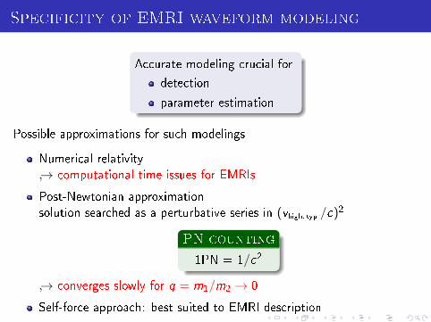
Specificity of EMRI waveform modeling
Accurate modeling crucial for
detection
parameter estimation
Possible approximations for such modelings
Numerical relativity
→ computational time issues for EMRIs
Post-Newtonian approximation
solution searched as a perturbative series in (vhigh. typ./c)2
PN counting
1PN = 1/c2
→ converges slowly for q = m1/m2 → 0
Self-force approach: best suited to EMRI description

Self-force approach
Covariant perturbative approach with ε = q
Method to obtain the SF equations of motion:
Expand the perturbed metric to order ε
g (ε)µν ≈ gµν + ε δg (1)
µν
Describe the point-like objects with some Tµν = εTµν(1) [yα, gαβ]
Solve the perturbed Einstein eqs with some regular Green function
Gµνregα′β′(x , x
′) = GµνR α′β′(x , x
′)− Gµνsingα′β′(x , x
′)highly non-trivialto construct withfull rigor

Self-force equations of motion
equations of motion = geodesic equations in gµν + ε δg (1) regµν
Duµ
dτ= f µ = O(q)
uµ
fµ
test particle orbit
SF orbit
(Delicate) numerical integration required in general
Use of Y `m-mode-sum regularization in practice
f reg =+∞∑`=0
[f` − A±L− B − CL−1
]− D with L = `+ 1/2

Interest of comparisons with PN calculations
PN and SF perturbative formalisms both fairly delicate
Both methods involve non-trivial regularizations
For PN:
eective representation of bodies by point-particle ⇒ dim-regtechnical Finite Part regularization to treat the eld multipole expansion
For SF:
Green function regularizationmode-sum regularization for δg (1)
µν (for example)
Insight about expansion properties
Comparison easiest using physical observables in conservative systems

1 Motivations, SF scheme
2 Detweiler redshift & comparison PN vs SF
3 PN computation of half-integral PN contributions

Case of exact circular motion
System of interest
small mass particle in circular orbit about a black hole
Consequences:
Helical killing vector: kµ → ∂µt + Ω ∂µφ in some class of gauges
Presence of incoming waves ⇒ conservative system
kµ
uµ∝ k
µ
light ring
I−
I+

Detweiler redshift observable
gravitational redshift
z = −kµuµ
Properties:
Simple interpretation for far-away observers along the axis
z−1 = u0
Gauge invariance property
z is a physical observable
⇒ u0 can be used for comparison with PN results
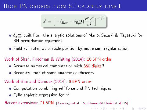
High PN orders from SF calculations I
u0 =[− (gµν + δg reg
µν )vµvν
c2
]−1/2δg regµν built from the analytic solutions of Mano, Suzuki & Tagasuki for
BH perturbation equations
Field evaluated at particle position by mode-sum regularization
Work of Shah, Friedman & Whiting (2014): 10.5PN order
Accurate numerical computation with 350 digits!!
Reconstruction of some analytic coecients
Work of Bini and Damour (2014): 8.5PN order
Computation combining self-force and PN techniques
Fully analytic expression for u0
Recent extensions: 21.5PN [Kavanagh et al. 15, Johnson-McDaniel et al. 15]

Half-integral PN order terms in u0
Definition
u0 =1√
1− 3y+q u0SF+O(q2)
PN parameter: y =(Gm2Ω
c3
)2/3
u0SF = −y +10∑n=1
αnyn+1 +
10∑n=4
βnyn+1 ln y +
10∑n=7
γnyn+1 ln2 y
− 13696
525πy13/2 +
81077
3675πy15/2 +
82561159
467775πy17/2
+ higher half-integral orders + y O(y11)
Notice the presence of terms ∝ 1/c2q+1
Why do they appear for this conservative dynamics?
How do we compute them using standard PN techniques?
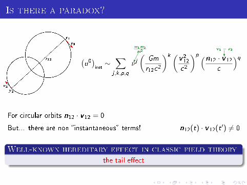
Is there a paradox?
v1
y1
v2
y2
r12
m1m2
m2v1 − v2(
u0)inst∼∑j ,k,p,q
ν j(
Gm
r12c2
)k (v212
c2
)p (n12 · v12
c
)q
For circular orbits n12 · v12 = 0
But... there are non-instantaneous terms! n12(t) · v12(t ′) 6= 0
Well-known hereditary effect in classic field theory
the tail eect

Tail effects
Tail wave
GW scattered on the
curvature of space-time
→ corresponds to a M ×ML
interaction in the waveform
Tail-of-tail wave
tail wave scattered on the
curvature of space-time
tail of tail: depends onthe source past
I+
I−
i+
i−
i0

1 Motivations, SF scheme
2 Detweiler redshift & comparison PN vs SF
3 PN computation of half-integral PN contributions
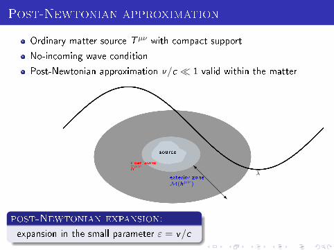
Post-Newtonian approximation
Ordinary matter source Tµν with compact support
No-incoming wave condition
Post-Newtonian approximation v/c 1 valid within the matter
source
exterior zoneM(hµν )
near zonehµν
λ
post-Newtonian expansion:
expansion in the small parameter ε = v/c
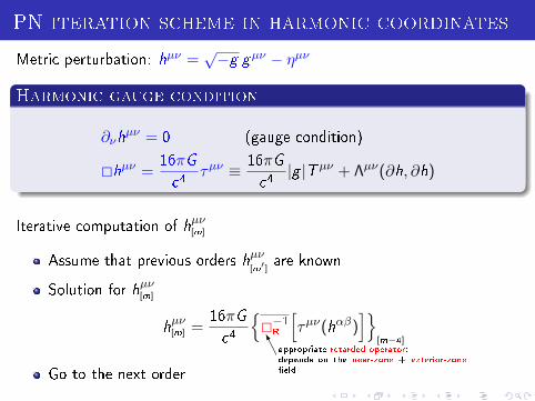
PN iteration scheme in harmonic coordinates
Metric perturbation: hµν =√−g gµν − ηµν
Harmonic gauge condition
∂νhµν = 0 (gauge condition)
2hµν =16πG
c4τµν ≡ 16πG
c4|g |Tµν + Λµν(∂h, ∂h)
Iterative computation of hµν[m]
Assume that previous orders hµν[m′] are known
Solution for hµν[m]
hµν[m] =
16πG
c4
2−1R
[τµν(hαβ)
][m−4]
appropriate retarded operator:depends on the near-zone + exterior-zoneeldGo to the next order

Structure of tail terms
Interactions involving knon stat ≥ 2 non-static moments ignored
M × ...×M × IP tail interactions in hµν
hαβM×···×M×IP
∼∑k,p,`,i
G kMk−1
c3k+pnL( rc
)`+2i∫ +∞
−∞du καβLP(t, u) I
(a)P (u)
nL = n
i1 ...ni` # of time der
dimensional analysis
angular-momentum selection rules
⇒
Only k = 3 contributes: M ×M ×moment = tail of tail
mass quadrupole: 5.5PN, 6.5PN, 7.5PN, ...
mass octupole: 6.5PN, 7.5PN, ...
mass hexadecapole: 7.5PN, ... Add 1PN for current moments
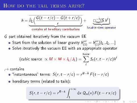
How do the tail terms arise?
h = ∂L
(G (t − r/c)− G (t + r/c)
r
)︸ ︷︷ ︸contains all hereditary contributions
+ 2−1inst[S nL]︸ ︷︷ ︸local-in-time operator
G part obtained iteratively from the vacuum EE
Start from the solution of linear gravity hµν(1) = hµν(1)[IL, JL, ...]
Solve iteratively the vacuum EE with an appropriate operator
(cubic source ∝ M ×M × IL/JL) =nite∑`
S`(r , t − r/c)nL
→ contains
instantaneous terms: S(r , t − r/c) = rB−k F (t − r/c)
hereditary terms (related to tails):
S(r , t − r/c) = rB−k∫ +∞
1dx Qm(x)F (t − r x/c)

Extraction of the hereditary tail part
We known that G (u) = FPB=0 Ck,`,m × (integral with a kernel τB)
⇒ Gtail-tail(u) ∝ G 3M2
cnResCk,`,m
∫ +∞
0dτ ln τ M
(a)L (u − τ)
Ansatz for the conservative part
Gcons(u) ∝ G 3M2
cnResCk,`,m
∫ +∞
0dτ ln τ
(M(a)L (u − τ) + M
(a)L (u + τ)
2
)
By matching: h00 = h00naive + h00tail-tail = −4Uc2
+ ...+ h00LO tail-tail + ...
Likewise for h0i , hij
⇒ Insertion into hµν[m] =
16πG
c4
2−1R
[τµν(hαβ)
][m−4]
→ couplings of U, ..., and hµνtail-tail

From the metric to u0
Structure of the n2PN-type gravitational field
hµνtail-tail ∼
∑G (a)cons(t) x
L∂φ
hµνtail-tail to be regularized at x = y1
Iij , Iijk , ... replaced by their explicit PN values
Integrals computed by using
x i12(t ± τ) = cos(Ωτ) x i12(t)± sin(Ωτ) v i12(t)/Ω
and ∫ +∞
0dτ ln τe iλτ = − π
2|λ|− i
λ(ln |λ|+γE)

Conclusion
We nd that there is no radial velocity
We conrmed the origin of the half-integral order conservative terms
We found full agreement with the SF results
Generalization beyond linear order in m1/m2 could be interesting