High Inflation and Real Wages

BENEDIKT BRAUMANN*

Empirical data show that real wages fall sharply during periods of high inflation.This paper suggests a simple general equilibrium explanation, without relying onnominal rigidities. It presents an intertemporal two-sector model with a creditchannel of monetary transmission. In this setting, inflation reduces real wagesthrough (1) a decline of the capital stock, and (2) a shift in relative prices. The twoeffects are additive and make the decline in real wages exceed the decline in percapita GDP. This mechanism may contribute to rising poverty during periods ofhigh inflation. [JEL E44]

High inflation is a powerful agent of redistribution. It can reduce the real valueof debt and tax revenues. In addition, it can impoverish large segments of the

population by eroding their earnings. Figure 1 shows four recent examples: Bolivia,Brazil, Ghana, and Mexico. From the beginning to the peak of high inflation,1 realwages fell by 55 percent in Bolivia, 61 percent in Brazil, 75 percent in Ghana, and48 percent in Mexico. It is notable that these countries shared similar experiences.Their economies have few elements in common, and inflation rates varied widely.This suggests a robust empirical pattern. Indeed, a wider sample of inflation crisesand more rigorous econometric tests confirm the relationship. In Braumann (2000),I studied 23 high inflation episodes in 17 different countries. The median declineof real wages was 24 percent. This and other macroeconomic patterns of high infla-tion are illustrated in Figure 2.

123

IMF Staff PapersVol. 51, No. 1

© 2004 International Monetary Fund

*Benedikt Braumann is an Economist in the IMF’s Western Hemisphere Department. He gratefullyacknowledges valuable comments from Bob Flood, Keiko Honjo, Monica Perez dos Santos, ThomasReichmann, Evan Tanner, Bob Traa, and two anonymous referees.

1Bruno and Easterly (1998) speak of an inflation crisis when annual inflation rises over 40 percent fortwo consecutive years. I will follow their definition here, as in Braumann (2000).

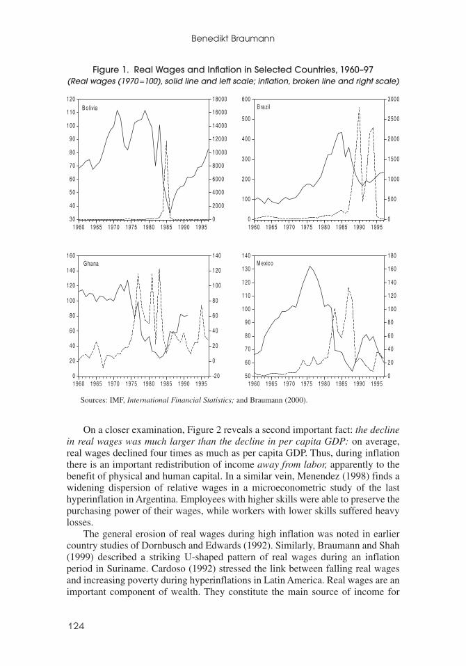
On a closer examination, Figure 2 reveals a second important fact: the declinein real wages was much larger than the decline in per capita GDP: on average,real wages declined four times as much as per capita GDP. Thus, during inflationthere is an important redistribution of income away from labor, apparently to thebenefit of physical and human capital. In a similar vein, Menendez (1998) finds awidening dispersion of relative wages in a microeconometric study of the lasthyperinflation in Argentina. Employees with higher skills were able to preserve thepurchasing power of their wages, while workers with lower skills suffered heavylosses.

The general erosion of real wages during high inflation was noted in earliercountry studies of Dornbusch and Edwards (1992). Similarly, Braumann and Shah(1999) described a striking U-shaped pattern of real wages during an inflationperiod in Suriname. Cardoso (1992) stressed the link between falling real wagesand increasing poverty during hyperinflations in Latin America. Real wages are animportant component of wealth. They constitute the main source of income for

Benedikt Braumann

124

30

40

50

60

70

80

90

100

110

120

0

2000

4000

6000

8000

10000

12000

14000

16000

18000

1960 1965 1970 1975 1980 1985 1990 1995

B olivia

0

100

200

300

400

500

600

0

500

1000

1500

2000

2500

3000

1960 1965 1970 1975 1980 1985 1990 1995

Brazil

0

20

40

60

80

100

120

140

160

-20

0

20

40

60

80

100

120

140

1960 1965 1970 1975 1980 1985 1990 1995

Ghana

50

60

70

80

90

100

110

120

130

140

0

20

40

60

80

100

120

140

160

180

1960 1965 1970 1975 1980 1985 1990 1995

M exico

Sources: IMF, International Financial Statistics; and Braumann (2000).

Figure 1. Real Wages and Inflation in Selected Countries, 1960–97(Real wages (1970 =100), solid line and left scale; inflation, broken line and right scale)

many households, especially for the less well-off. The behavior of real wages there-fore has a direct bearing on income distribution and the level of poverty.

Why do real wages decline during high inflation? Macroeconomic theory hasgiven surprisingly little attention to this phenomenon. A commonly heard argumentrelies on backward-looking indexation. As inflation accelerates, the adjustment ofnominal wages lags behind, and real wages fall. While this argument may explainthe initial impact of surprise inflation, it has several weaknesses over the longerrun. First, falling real wages might, all things being equal, lead to higher labordemand and activity. However, during high inflation one observes a decline inactivity (see Figure 2 for real GDP and employment).2 Second, the argument relieson money illusion on part of the workers. Rational workers would soon discover theerosion of their real wages, and negotiate accordingly. My previous paper (2000)

HIGH INFLATION AND REAL WAGES

125

2Braumann (2000) also finds a negative effect of inflation on employment. A large literature on sta-bilization finds similar correlations; see, for example, the survey by Rebelo and Végh (1995).

7 0

7 5

8 0

8 5

9 0

9 5

1 0 0

1 0 5

1 1 0

1 1 5

t - 6 t - 5 t - 4 t - 3 t - 2 t - 1 t t +1 t +2 t +3 t +4 t +5 t +6

GD P p e r c a p it a

R e a l wa ge s

t - 6 = 1 0 0

9 0

9 5

1 0 0

1 0 5

1 1 0

1 1 5

1 2 0

t - 6 t - 5 t - 4 t - 3 t - 2 t - 1 t t + 1 t + 2 t + 3 t + 4 t + 5 t + 6

C o n sum p t io n

E m p lo y m e n t

t - 6 = 1 0 0 , p e r c a p it a

0

2 0

4 0

6 0

8 0

1 0 0

1 2 0

1 4 0

t - 6 t - 5 t - 4 t - 3 t - 2 t - 1 t t +1 t +2 t +3 t +4 t +5 t +6

I n f la t io n , in p e r c e n t

6 0

7 0

8 0

9 0

1 0 0

1 1 0

1 2 0

1 3 0

t - 6 t - 5 t - 4 t - 3 t - 2 t - 1 t t +1 t +2 t +3 t +4 t +5 t +6

I n v e st m e n t

R e a l M 2

t - 6 = 1 0 0 ,p e r c a p it a

Figure 2. Macroeconomic Patterns in High Inflation Episodes(23 episodes, median values)

Source: Braumann (2000).

found that the average duration of an inflation crisis is seven years. This seemsample time to correct errors in price expectations. Finally, the decline in real wagesoccurred even during repeated and closely spaced inflation crises—for example inArgentina, Brazil, and Uruguay. Learning effects should have eliminated money illu-sion by the second or third inflation crisis within a generation.

It therefore seems possible that the fall of real wages during high inflation isan equilibrium phenomenon. To explore this hypothesis further, this paper intro-duces a simple general equilibrium model. There is no uncertainty and no asym-metry of information, and there are no nominal rigidities. All markets clear, andinflation is fully expected. The idea is to explain the stylized facts of Figure 2 withas few and as standard assumptions as possible. The basic neoclassical model ofmonetary growth serves as a point of departure, with the addition of a second sec-tor of production. This allows us to derive a relative price and to analyze the redis-tribution of income. The model yields an unambiguous and strong decline of realwages during inflation, and traces many other stylized facts reasonably well. Thepaper begins with an intuitive outline of the argument, before presenting the modelin full detail. Then, it simulates both a permanent and a temporary increase ininflation and compares a central prediction of the model with the data. In the lastsection, the paper discusses the social consequences of the sharp fall in real wages,and then concludes.

I. Intuition

The intuitive results of the model can be summarized quickly. Let us assume aneoclassical two-sector economy that produces consumer and investment goods.There are two factors of production: capital and labor. Labor supply is exogenous,and capital is accumulated through the savings of households. The economy isclosed, and all savings are invested in physical capital. The two sectors of pro-duction differ in factor intensities: consumer goods are more labor intensive thaninvestment goods. Finally, a formal banking sector is needed to intermediate sav-ings and investment. Reserve requirements create a transmission mechanism frommonetary policy to the real economy. The structure could be classified as anintertemporal Heckscher-Ohlin model with a credit channel.

Assume now that the government begins to hand out lump-sum transfers andincurs a budget deficit. To finance the deficit, it resorts to money creation. As aresult, inflation rises from zero to µ percent a year. This leads to financial disin-termediation. If reserve requirements are not (fully) remunerated, deposit rates arenot indexed and may turn negative in real terms. As inflation increases, house-holds withdraw funds from the financial system and force banks to cut real credit.

With less credit available, investment contracts, and the capital stock declinesover time. A lower capital stock reduces GDP and makes labor less productive.Therefore, labor demand declines and real wages fall.

In a two-sector economy, this effect is reinforced by a shift in the compositionof GDP. Assume for a moment that relative prices are constant. In this case, theRybczynsky theorem holds. A lower capital stock reduces the supply of the capital-intensive good, while the supply of the labor-intensive good expands. The capital-

Benedikt Braumann

126

intensive good (investment) becomes scarce; the labor-intensive good (consump-tion) becomes abundant.

Inflation thus leads to a change in relative prices. To clear the markets, the rel-ative price of the labor-intensive good declines. In a two-sector economy, theStolper-Samuelson theorem provides a link from goods prices to factor prices. Asthe price of the labor-intensive good declines, real wages must fall. In fact, the the-orem predicts that real wages fall by more than relative prices. This is a secondnegative effect on real wages, which magnifies the first one. In combination, thetwo effects can be empirically important. While the lower capital stock leads to aproportional decline in output and real wages, the shift in relative prices makesreal wages “overshoot.” This is the model’s interpretation of the stylized fact thatreal wages decline by more than per capita GDP.3

II. The Model

This section describes the model in detail. As noted above, a Heckscher-Ohlinsupply side is combined with a credit channel and solved in a context of inter-temporal optimization. The model assumes rational expectations for all agents,perfect competition, and the absence of nominal rigidities and uncertainty. Theresult is a dynamic general equilibrium, which can be analyzed with standard toolsof macroeconomics, such as phase diagrams. The aim of this section is to explorehow far a simple structure can go in explaining the observed patterns of real wagesand inflation.

The model can be set into the general context of monetary growth theory, whichstudies the medium- and long-term effects of inflation on real variables. A classicalsurvey of monetary growth theory is given by Orphanides and Solow (1990), and amore recent one by Capasso (1997). The discussion was initiated by Tobin (1965),who added money to the Solow growth model. His model showed that inflation hada positive effect on growth, since it induces people to lower money balances andstep up capital accumulation. The Tobin effect has unsettling policy implications, andwas contested by Sidrauski (1967) on theoretical grounds: first, it postulates exoge-nous savings and second, it provides no microfoundations for money holdings.Tobin assumed ad hoc that people hold money as an asset, despite the fact thatcapital always yields higher returns (unless there is deflation). In contrast,Sidrauski included real balances in the utility function, and solved the model withdynamic optimization. As a result, inflation no longer had any effects on real vari-ables but was found to be superneutral.

Stockman (1981) noted that Sidrauski’s treatment of money holdings was stillnot satisfactory. Money does not yield utility as such but is used mainly to facili-tate transactions. When Stockman introduced a cash-in-advance constraint to themodel, inflation turned out to have negative effects on capital accumulation and

HIGH INFLATION AND REAL WAGES

127

3In an open-economy setting, the same forces can be expected to work. Investment goods can belinked to tradables, and consumer goods to nontradables. Nontradable goods are usually more labor inten-sive than tradables, and their relative price is the real exchange rate.

growth. In this setting, inflation acts as a tax on transactions, in particular oninvestment. The Tobin effect was thus turned on its head.

Overall, the direction of the real effects depends crucially on how moneyholdings are modeled. Empirical papers generally support a negative effect ofinflation on growth—see, for example, Ghosh and Phillips (1998)—and suggestthat the transaction function of money is most important. The model presentedbelow follows this line of argument by focusing on the role of the banking sectorin financing investment. As in Stockman’s model, inflation has a negative impacton the capital stock—and, as a consequence, on real wages.

On a more specific level, the theoretical literature on real wages and high infla-tion is thin. Helpman and Leiderman (1989) develop a model in which staggeredwage and price contracts lead to a positive correlation between inflation and realwages. Nonlinearities in the wage bargaining process accelerate inflation whenunions increase their real wage demands. The results of the model contradict theempirical evidence presented above. Also, the causality is implausible, as inflationneeds a monetary expansion to keep going.

Since the late 1980s, two-sector models have sometimes been used to analyzethe real effects of money. A first series of papers, exemplified by Calvo (1986) andCalvo and Végh (1993), concentrated on disinflation programs, which often led toreal appreciations and current account deficits. These models stressed credibilityproblems of the government (the “temporariness” hypothesis) and focused on thedemand side of the economy. The supply side was treated in a rudimentary way,usually by assuming fixed endowments. Since these models abstracted from inputfactors, they could not explain the behavior of real wages.4

Closer to our question are papers by Roldós (1995), Rebelo and Végh (1995),Uribe (1997), and Lahiri (2001), who also examine disinflation programs. Theseauthors use the specific-factor model for the supply side, which is, like Heckscher-Ohlin, a workhorse of external trade theory. Although the specific-factor modelproduces a decline in real wages during high inflation, its magnitude falls short ofthe evidence seen in Figures 1 and 2. This is due to the so-called neoclassicalambiguity: changes in relative prices have little or ambiguous effects on realwages, which are the reward of the mobile factor labor. They have strong effectson the rewards of specific factors. The decline of real wages in such models ismostly due to a decrease of the capital stock.

A Heckscher-Ohlin structure allows both capital and labor to shift betweensectors, and yields unambiguous results for factor prices. The fact that this struc-ture is not used more frequently is unfortunate, since the Heckscher-Ohlin modelintegrates easily into the kind of general-equilibrium framework that is a staple ofmacroeconomics. One of the few examples in the literature is Stockman (1985),who uses a Heckscher-Ohlin approach to study the real effects of inflation on tradepatterns (but not on real wages). The approach is sometimes criticized on thegrounds that intersectoral factor mobility requires a lot of time. While this servesas a caveat to interpret our results in a strictly qualitative way, most of the fol-lowing analysis in fact concerns patterns that span up to a decade.

Benedikt Braumann

128

4See Braumann and Shah (1999) for a case study on inflation in Suriname and the limits of the tem-porariness approach.

In the model below, the supply side consists of two sectors of production, onefor consumer goods and one for investment goods. There are two factors, labor andcapital, and both are mobile across sectors. Consumer goods are labor intensive,and investment goods are capital intensive. Factor endowments and output pricesdetermine the relative supply of each good. The output of a sector expands if its rel-ative price increases. It also expands with an increase in the endowment of the inputfactor that is used more intensively. Therefore, the first step in solving the model isto derive aggregate supply. The resulting transformation curve links sectoral pro-duction to relative prices and factor endowments. The demand side of the modelconsists of households that maximize utility and decide on consumption and sav-ings. Aggregate demand selects the equilibrium price on the transformation curve.

Finally, monetary shocks are transmitted to the real economy via a credit chan-nel. Investment needs to be financed in the formal banking sector.5 This assump-tion is in line with empirical observations in Latin America, and also in many otherparts of the world. A credit channel produces similar results to a cash-in-advanceconstraint on investment, as in Uribe (1997), but may be more empirically appeal-ing. The size of the formal financial sector is determined by the amount of deposits,which depends on the real interest rate paid by banks. As the real deposit ratedeclines, the amount of deposits falls and the volume of credit contracts. With lesscredit available, firms are forced to cut their investment plans.

The government finances its deficit through the inflation tax. The tax base is cen-tral bank money, which is the sum of currency and reserve requirements of banks.In the following, we will assume that all central bank money consists of reserverequirements. To collect seignorage, the state pays no interest on reserve require-ments. If inflation is greater than zero, banks thus incur negative real returns onan important part of their assets. This is the first incidence of the inflation tax.Competitive banks pass this tax onto households by lowering deposit rates belowlending rates. With high inflation, deposit rates may become negative in realterms. Inflation combined with unremunerated reserves is an element of distor-tion or financial repression in the economy.

Figure 3 shows real deposit rates, real M2 (deposits and cash), and real creditto the private sector during the 23 inflation episodes mentioned above. In practice,financial repression comes in many forms. On average, the countries in the sampleimposed reserve requirements of 35 percent. Argentina, Chile, and Venezuela hadrequirements of up to 100 percent. Several countries accompanied reserve require-ments with explicit ceilings on deposit rates. Thus, real deposit rates turned sharplynegative during high inflation. As a result, households withdrew funds from the for-mal banking system, causing real M2 and real credit to contract. High inflation ledto a marked decline of financial intermediation.

For the sake of simplicity, we assume all seignorage revenues are reimbursedto the private sector via lump-sum transfers. This allows us to concentrate on therelative price distortions generated by the inflation tax. By excluding wealth effects,we can simplify the algebra without losing substance. Wealth effects lead to a reduc-tion of steady-state consumption, but leave the qualitative effects on real wagesunchanged.

HIGH INFLATION AND REAL WAGES

129

5Bernanke and Gertler (1995) present a survey of the credit channel of monetary transmission.

Firms: Cost Minimization and Pricing

Firms in both sectors combine labor Nt and capital Kt to produce output. The con-sumer good Ct is assumed to be labor intensive, the investment good It is capitalintensive. Labor and capital are mobile between the two sectors. Labor is suppliedinelastically by households and normalized to 1. The accumulation of capital isendogenous, and will be determined by the utility maximization of households. Inparticular, the following sectoral production functions are used:

(1)

(2)I K Nt I t I t= −, , ,1 α α

C K Nt C t C t= −, ,

α α1

Benedikt Braumann

130

-40

-35

-30

-25

-20

-15

-10

-5

0

5

t-6 t-5 t-4 t-3 t-2 t-1 t t+1 t+2 t+3 t+4 t+5 t+6

Real deposit rate, in percent

50

60

70

80

90

100

110

120

130

t-6 t-5 t-4 t-3 t-2 t-1 t t+1 t+2 t+3 t+4 t+5 t+6

Credit to the private sector

M2

t-6 = 100,real per capitalevels

Figure 3. High Inflation and the Financial System(Median values of 23 inflation crises)

Source: IMF, International Financial Statistics.

where α is strictly smaller than 0.5. The sectoral production functions are mirrorimages of each other. This symmetry is introduced for the sake of simplicity andto save on notation. Markets are perfectly competitive and prices are flexible. Theprice of investment goods is chosen as numéraire. The variable pt denotes the rel-ative price of the consumer good, and can be thought of as the real exchange ratein an open-economy setting. Labor earns a real wage wt and capital, a rental ratert. Factor prices are equalized across the economy, since both factors are perfectlymobile. Omitting the time subscript, cost minimization by firms leads to

(3)

Next, we define the input-output coefficients as ni = Ni/i and ki = Ki/i, with i = C,I. Inserting the minimum-cost combinations and carrying out a total differentiationyields:

(4)

(5)

(6)

(7)

where hats denote deviations from the initial steady state, e.g., C = (C − C*)/C*.Perfect competition ensures that prices are equal to unit costs and profits areeliminated:

(8)

Differentiating equation (8) and substituting equations (4)–(7) yields

(9)

(10)

By subtracting equation (10) from equation (9), one arrives at the Stolper-Samuelson relation:

(11)

where p denotes the relative price of the labor-intensive consumer good. The fol-lowing two expressions for factor prices follow as a corollary of equations (9),(10), and (11):

(12)ˆ ˆw p= −

−1

1 2

αα

ˆ ˆ ˆ ,p w r= −( ) −( )1 2α

ˆ ˆ ˆ.p w rI = + −( )α α1

ˆ ˆ ˆp w rC = −( ) +1 α α

p wn rk i C Ii i i= + =, , .

ˆ ˆ ˆ ,k w rI = −( )α

ˆ ˆ ˆk w rC = −( ) −( )1 α

ˆ ˆ ˆn w rI = − −( ) −( )1 α

ˆ ˆ ˆn w rC = − −( )α

K

N

w

r

K

N

w

rC

C

I

I

=−

= −αα

αα1

1and .

HIGH INFLATION AND REAL WAGES

131

(13)

Resource Constraints

Flexible factor prices ensure that labor and capital are always fully employed.The input-output coefficients can be used to determine the allocation of the twofactors among the two sectors of production. The full-employment conditions canbe written as

(14)

(15)

To save on notation, we shall work with a symmetric initial steady state. FromN = 1, p = r = 1, and C = I, it follows that KC/K = α, NC/N = 1 − α.6 Differentiate(14) and (15) using these assumptions and equations (4)–(7) to obtain

(16)

(17)

Subtracting equation (16) from (17) and inserting the Stolper-Samuelson relation(11) gives

(18)

This equation summarizes the supply side of the economy and can be interpretedas a transformation curve. If factor supplies are constant, the economy moves alongthe transformation curve according to changes in relative prices. The production ofa good increases if its relative price increases. On the other hand, the transforma-tion curve shifts out if factor supplies expand. A particularly interesting situationarises when relative prices are constant. In this case, equation (18) reduces to theRybczynsky theorem: if the supply of a factor increases (e.g., capital), the sectorusing this factor intensively expands (e.g., investment goods) and the other sectorcontracts (consumer goods). To determine the equilibrium relative price and output,we turn to the demand side.

Financial System

The financial system intermediates savings to finance investment. Householdsdeposit their savings in banks. Deposits Dt earn an interest rate iDt. Banks use these

1 24 1

1 2−( ) −( ) = − −( )

−+ −( )α α α

αˆ ˆ ˆ ˆ ˆ .I C p K N

ˆ ˆ ˆ ˆ ˆ.K w r C I= −( ) −( ) + + −( )2 1 1α α α α

ˆ ˆ ˆ ˆ ˆN w r C I= − −( ) −( ) + −( ) + =2 1 1 0α α α α

K K K k C k IC I C I= + = + .

N N N n C n IC I C I= + = + = 1

ˆ ˆ.r p= −−α

α1 2

Benedikt Braumann

132

6In this symmetric steady state, the equation for capital accumulation (26) yields w = C = K. From costminimization in the consumer goods industry follows that rKC = α/(1 − α) wNC. Equating revenues and totalcosts, wNC + rKC = C, and combining this with the two relations before yields KC = α and NC = 1 − α.

deposits to extend credit Crt at an interest rate iCrt. However, they are also required

to hold a fraction ρ of deposits as reserves Rt at the central bank, earning no inter-est, iRt = 0. Thus, the balance sheet of banks reads

and profits are

Perfect competition in the banking sector drives profits down to zero. From this itfollows that

Higher reserve requirements widen the spread between nominal lending anddeposit rates. Deposit rates are not completely indexed to inflation, since a goodpart of the bank’s assets earns no interest at all. Thus, at high levels of inflationreal deposit rates become negative. In the following, we will simplify the algebraby assuming ρ = 1, or reserve requirements of 100 percent, as in Argentina, Chile,and Venezuela (see above). Nominal deposit rates become zero, and deposits arefully backed by central bank money.

Households

The economy is inhabited by a large number of identical households, which deriveutility from consuming the consumer good Ct. They maximize the following log-arithmic utility function

(19)

where β is the discount factor. Individuals hold two different types of assets, capi-tal Kt and deposits Dt. They receive income from wages wt, renting out capital rt

and government transfers Trt. Labor supply is inelastic and normalized to 1. Capitalis assumed to depreciate within one period. Since the price of the investment goodis taken as numéraire and fixed at unity, all real quantities are expressed in terms ofinvestment good prices. Accordingly, households face the budget constraint

(20)

Households accumulate deposits in the banking system to finance investment atthe end of each period. Investment turns into productive capital at the beginningof the next period. Banks pool the deposits and organize the financing of large-scale projects. Such projects must be financed by a large formal banking sector

KD

Pw r K Tr

D

Pp Ct

t

tt t t t

t

tt t+

−+ = + + + −11 .

U Ct

tt=

=

∞

∑ β0

ln ,

i itD

tCr= −( )1 ρ .

Π t tCr

t tR

t tD

ti Cr i R i D= + − .

D Cr Rt t t= +

HIGH INFLATION AND REAL WAGES

133

that is based on central bank money, and not by an informal curb market. To makethis link explicit, we impose a deposit-in-advance constraint on investment. Tostart an investment project, households need to maintain deposits in the bankingsystem:

(21)

Investment is thus related to the size of the formal financial sector. Since capitalyields a larger return than deposits, the constraint will hold with equality through-out the model. As noted above, we assume reserve requirements of ρ = 1, whichimplies that Dt = Rt. Deposits are fully backed by central bank money. Denotingmonetary growth as µt, the following expression can be derived:

(22)

Making use of the last two equations in the budget constraint (20), solving (20) forCt, substituting the results in equation (19) and maximizing with regard to Kt+1

yields the Euler equation:

(23)

Differentiating around the steady state leads to

(24)

Government

The only expenditures of the government are transfers to households. Since thereare no taxes, the resulting deficit is completely financed by money creation. Thebudget deficit is thus the source of monetary growth, which in turn determines theinflation rate. Algebraically, the budget constraint of the government is given by

(25)

Next, we consolidate the government and household sectors by substituting for Trt

in equation (20). This leads to the economy-wide equation of capital accumulation:

(26)

Differentiating and linearizing equation (26) around the steady state yields

K w r K p Ct t t t t t+ = + −1 .

TrR R

P

D

PKt

t t

t

t

tt= − = −( ) −( )− −+

1 111 1µ µ .

ˆ ˆ ˆ ˆ ˆ ˆ .C C p p rt t t t t t+ + += + − + −1 1 1 µ

C

C

p

p

rt

t

t

t

t

t

+

+

+=1

1

1

βµ.

D

PKt

tt tµ +1.

D

PI Kt

tt t

−+≥ =1

1.

Benedikt Braumann

134

(27)

By subtracting Kt from equation (27) we obtain an equation that expresses aggre-gate demand conditions in the economy:

(28)

General Equilibrium

The relative price pt can be determined by equating aggregate demand (28) andaggregate supply (18). After substituting equations (12) and (13) for wt and rt inequation (28) and eliminating (It − Ct), the relative price becomes

(29)

This expression can be used to derive the equations that determine the dynamicbehavior of the model. The equation for capital accumulation becomes

(30)

The Euler equation (24) determines the dynamics of consumption. After substitut-ing for rt+1, pt, and pt+1, and collecting terms, it reads

(31)

With these two equations of motion, a phase diagram can be constructed. Thedemarcation lines are

(32)

(33)

A graphical interpretation of the model is given in the phase diagram of Figure 4.The equilibrium is a saddle point and the stable transition path has a positive slope.In this economy, money is not superneutral. The parameter µ enters the demarca-tion line for consumption (33) as a shift factor. As inflation increases, this lineshifts up, causing the capital stock to decline and output to contract.

III. The Effects of Inflation

A Permanent Increase in Inflation: Long-Run Effects

Assume that the government increases transfer payments to households perma-nently. The resulting fiscal deficit is financed by money creation. As a first step, ithelps to abstract from short-run dynamics and concentrate on the new steady state.

∆ ˆ : ˆ ˆ .C C K= = + −( )0 2 1µ α α

∆ ˆ : ˆK C= =0 0

ˆ ˆ ˆ .C C Kt t t+ = − +−

−−

−1

2 21

1 12

α αα

αα

αµ

ˆ ˆ ˆ .K K Ct t t+ = −1

ˆ ˆ ˆ .p K Ct t t= −−( )

+ −( )

−( )1 2

2 1

1 2

2 1

2αα

αα α

ˆ ˆ ˆ ˆ ˆ ˆ ˆ .I C w r K p Ct t t t t t t− = + + − − 2

ˆ ˆ ˆ ˆ ˆ ˆ .K w r K p Ct t t t t t+ = + + − −1

HIGH INFLATION AND REAL WAGES

135

The monetary expansion drives up the inflation rate from 0 to µ. The effects on thereal economy are shown in Figure 5. As the demarcation line for consumptionshifts up, the economy moves to the new equilibrium 2. Solving equations (32)and (33) yields the following steady-state values:

Inflation has negative effects on almost all macroeconomic variables. An inclusionof wealth effects would result in a negative effect on consumption as well. Thesteepest decline occurs in the capital stock (and for that matter, investment), fol-lowed by real wages. Since the model is highly stylized, these results are of aqualitative nature. Nevertheless, one can perform a little numerical exercise, forexample, by calibrating the parameter α to 1/3, as suggested by the macro literatureon developing countries (e.g., Mendoza and Uribe, 1999), and µ to 2.2, the medianinflation peak (123 percent) in the empirical sample. The ordering of the inflationeffects is closely in line with the empirical values: the decline in relative prices istwice as deep, and the decline in real wages four times as deep as the decline in

ˆ

ˆ

ˆ

ˆ ˆ ˆ ˆ

ˆ

ˆ

K

w

p

Y I p C

C

r

= − −( )

= − −( )

= − −( )

= − −( ) = + +

=

=

2 1

1

1 2

1 2 2

0

α µ α

α µ α

α µ α

α µ α

µ

Benedikt Braumann

136

k

c

∆k = 0

1

∆c = 0

Figure 4. The Dynamics of the Model in the c/k-Space

GDP. In the sample of 23 inflation episodes, real GDP declines by 6 percent, therelative price of investment goods by 10 percent, and real wages by 24 percent.The simulation gives a decline of real GDP of 1.1 percent, which falls short of theobservations. However, this magnitude is quite sensitive to the choice of the tech-nology parameter α, and the symmetry imposed on the two sectors of production.The model imposes an average capital intensity of 0.5, which is a high value. Witha lower average capital intensity, especially with a lower α in the labor-intensivesector, the decline in GDP deepens.

As noted above, the large fall in real wages is the result of two mutually rein-forcing effects. First, higher inflation leads to a decline in the capital stock and toa lower marginal product of labor. Second, the sectoral composition of outputchanges, producing an excess supply of labor-intensive goods. This causes rela-tive prices to decline, and via the Stolper-Samuelson theorem, real wages to fall.Equation (11) expresses the Stolper-Samuelson effect: a fall in relative pricesleads to a (magnified) fall in real wages. As the labor-intensive sector contracts, itreleases a large number of workers, which cannot easily be absorbed by the capital-intensive sector as this contracts as well. Accordingly, a large adjustment of realwages is necessary to clear the labor market.

Short-Run Effects and Transition Dynamics

The severe contraction that inflation causes over the medium term is often maskedby an initial short-run boom. This has been a familiar pattern in several LatinAmerican countries, where governments used inflationary policies to engineer

HIGH INFLATION AND REAL WAGES

137

k

c

∆c = 0

∆k = 0 1

1′

2

∆c′ = 0

Figure 5. A Permanent Increase in Inflation

a redistribution of income towards urban labor. Often, such policies resulted inimmediate rapid GDP growth and real wage gains. The following quotes from acollection of articles in Dornbusch and Edwards (1992) give a vivid account ofthis phenomenon. Sturzenegger (1992, p. 80) writes about Perón’s third adminis-tration in Argentina in 1974:

After a year, the results of the program had been so spectacular that eventhose most strongly opposed to the government had to give credit to theeconomic policy being implemented.

Larraín and Meller (1992, p. 194) note about Allende’s socialist-populist experi-ment in Chile:

The Chilean economy experienced an unprecedented boom in 1971. Thisgenerated a . . . sense of total success among Unidad Popular leaders.The labor share in GDP increased from 52.2% (1970) to 61.7% (1971),. . . with an overall average [increase in real wages] of 22.3%.

Lago (1992, p. 275) describes the initial phase of Alán García’s rule in Peru asfollows:

After a few months of initial sluggishness, the response of the economyto the program was an unprecedented output expansion. Real wages grewby 24 percent over the two-year period [of 1986–87]. Private sector con-fidence in and support of the government’s economic policies could onlybe described as unanimous.

A short-term boom and its painful collapse is also implied in the transition dynam-ics of the model. Figure 6 shows the trajectories of the main macro variables overtime. By taxing financial intermediation, inflation raises the effective price ofinvestment goods on impact. Households react by investing less and consumingmore. Consumption jumps from steady state 1 to point 1′. Since total factor sup-plies are fixed in the short run (capital is the state variable), production cannotincrease as fast as demand. A shortage of consumer goods develops, leading to anincrease in their relative price. Because consumer goods are labor intensive, realwages temporarily rise via the Stolper-Samuelson effect.

However, the brief consumption boom comes at the expense of lower invest-ment, and therefore of future output. From the second period onward, the capitalstock declines, and the economy contracts. Everything now works against labor,and the initial gains dissipate quickly. The long-run consequences were describedabove: in the new steady state, the levels of GDP and real wages are lower thanbefore. Thus, the attempt to redistribute income via expansionary policies is self-defeating, and wage earners are the principal losers from inflation.

A Temporary Increase in Inflation

A weakness of the previous analysis is the assumption that inflation increases per-manently. Historical experience suggest that high inflation seldom lasts for long.The median duration of 23 high inflation episodes in my previous (2000) paper

Benedikt Braumann

138

HIGH INFLATION AND REAL WAGES

139

Time t0

Real interest rate

r

Time t0

Consumption

c

Time t0

Relative price of labor-intensive good

p

Time t0

Capital stock

k

Time t0

Money growth

µ

Time t0

GDP

wy

Real wages

Figure 6. Dynamic Effects of a Permanent Increase in Inflation

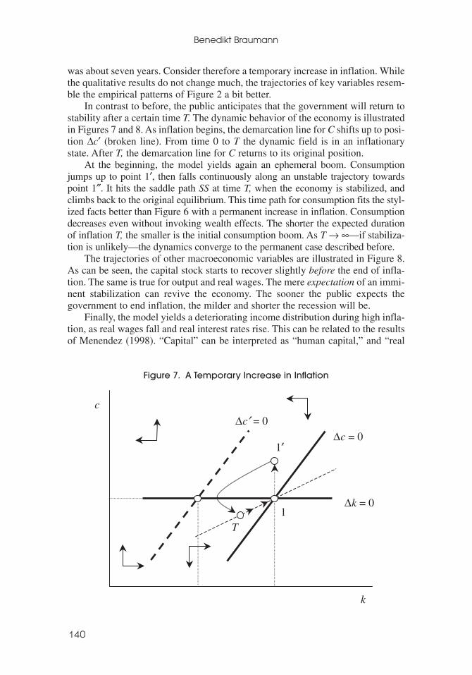
was about seven years. Consider therefore a temporary increase in inflation. Whilethe qualitative results do not change much, the trajectories of key variables resem-ble the empirical patterns of Figure 2 a bit better.

In contrast to before, the public anticipates that the government will return tostability after a certain time T. The dynamic behavior of the economy is illustratedin Figures 7 and 8. As inflation begins, the demarcation line for C shifts up to posi-tion ∆c′ (broken line). From time 0 to T the dynamic field is in an inflationarystate. After T, the demarcation line for C returns to its original position.

At the beginning, the model yields again an ephemeral boom. Consumptionjumps up to point 1′, then falls continuously along an unstable trajectory towardspoint 1″. It hits the saddle path SS at time T, when the economy is stabilized, andclimbs back to the original equilibrium. This time path for consumption fits the styl-ized facts better than Figure 6 with a permanent increase in inflation. Consumptiondecreases even without invoking wealth effects. The shorter the expected durationof inflation T, the smaller is the initial consumption boom. As T → ∞—if stabiliza-tion is unlikely—the dynamics converge to the permanent case described before.

The trajectories of other macroeconomic variables are illustrated in Figure 8.As can be seen, the capital stock starts to recover slightly before the end of infla-tion. The same is true for output and real wages. The mere expectation of an immi-nent stabilization can revive the economy. The sooner the public expects thegovernment to end inflation, the milder and shorter the recession will be.

Finally, the model yields a deteriorating income distribution during high infla-tion, as real wages fall and real interest rates rise. This can be related to the resultsof Menendez (1998). “Capital” can be interpreted as “human capital,” and “real

Benedikt Braumann

140

k

c

∆c = 0

∆k = 0 1

1′

∆c′ = 0

T

Figure 7. A Temporary Increase in Inflation

HIGH INFLATION AND REAL WAGES

141

Time

Relative price of labor- intensive good

p

t0 T Time

Consumption

c

Time

Capital stock

k

t0 T Time t0 T

Money growth

µ

Time

GDP

wy

Real wages

t0 T Time

Real interest rate

r

t0

T

t0 T

Figure 8. Dynamic Effects of a Temporary Increase in Inflation

interest rates” as the salary of high-skilled professionals. During high inflation,real interest rates and real wages do in fact move apart.

An Empirical Illustration of Relative Price Effects

A central mechanism in the model is the decline of the relative price of labor-intensive goods. It ultimately causes the “overshooting” of real wages. Does a rel-ative price effect show up in the data? While this is not the place for an exhaustiveempirical study, a brief illustration may be useful. Since there is no straightfor-ward empirical equivalent to the relative price of the model, approximations haveto be constructed. A first proxy is the real internal exchange rate (defined as non-tradable over tradable prices). Nontradables are generally more labor intensivethan tradables. In Braumann (2000), I proxied tradables by the price of clothingand nontradables by the price of housing services in the consumer price index.During the 23 inflation crises analyzed in that paper, the median internal realexchange rate declined by 35 percent (Figure 9). Another proxy for the relativeprice is the ratio of consumption to investment deflators, as taken from thenational accounts. Owing to data restrictions, the sample is limited to 15 inflationcrises. Figure 9 shows that the relative price of consumption declined by about 10percent during high inflation. In a rough and preliminary way, the data seem tosupport the relative price effect of the model.

IV. Real Wages and Poverty

The model above can be applied to a closely related question: Can lowering infla-tion reduce poverty? The wave of market-oriented reforms in Latin America dur-ing the late 1980s and early 1990s coincided with a sharp increase in poverty in theregion. Based on casual evidence, it has been argued that the poor bore the bruntof the adjustment process. Poverty was seen as the dark side of market-orientedreforms. Monetary stabilization, downsizing of the government, selling of publicassets, and trade liberalization were all portrayed as having regressive effects onincome distribution.7

The model of this paper suggests a different perspective. Both data and theorysupport the notion that inflation leads to a sharp decline in real wages. If realwages are an important part of lower-class income, they can be expected to corre-late with the level of poverty, as Cardoso (1992) argues. Therefore, it seems likelythat not adjustment itself but the previous bout of high inflation caused the rise inpoverty. Inflation led to a sharp decline in real wages, pushing many householdsbelow the poverty line.

Figure 10 combines the inflation rates in four countries with recent time seriesdata on poverty from ECLAC (1999) and Londoño and Székely (1997). Poverty ismeasured as the percentage of population that lives on less than US$2 a day. Despitesome gaps in the data record, a clear pattern emerges: poverty peaked roughly at theheight of the inflation maximum. After the end of inflation, real wages rebounded

Benedikt Braumann

142

7For an explicit and quite thorough presentation of this argument see Morley (1995).

and poverty decreased. This picture continues to hold in a wider sample of observa-tions. Figure 11 shows the median poverty rate of six inflation crises in Argentina,Brazil, Costa Rica, Mexico, Peru, and Uruguay. Poverty peaks at time t, the yearof the inflation maximum. The sharp decline of real wages was instrumental inincreasing poverty.

A more rigorous study by Bulír (2001) confirms this finding. The author ana-lyzes the question of why income distribution in Latin America is more unequal thanin Asia. He finds that much of this difference is due to higher inflation rates in LatinAmerica, after controlling for variables like per capita income and public transfers.

HIGH INFLATION AND REAL WAGES

143

50

60

70

80

90

100

110

t-6 t-5 t-4 t-3 t-2 t-1 t t+1 t+2 t+3 t+4 t+5 t+6

Relative price of nontradables

t-6 = 100

85

90

95

100

105

110

t-6 t-5 t-4 t-3 t-2 t-1 t t+1 t+2 t+3 t+4 t+5 t+6

Ratio of consumption to investment deflator

t-6 = 100

Figure 9. Relative Price of Labor Intensive GoodsDuring High Inflation

(Median behavior of two empirical proxies)

Sources: Braumann (2000); and UN National AccountsStatistics.

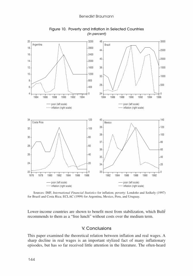
Lower-income countries are shown to benefit most from stabilization, which Bulírrecommends to them as a “free lunch” without costs over the medium term.

V. Conclusions

This paper examined the theoretical relation between inflation and real wages. Asharp decline in real wages is an important stylized fact of many inflationaryepisodes, but has so far received little attention in the literature. The often-heard

Benedikt Braumann

144

4

6

8

10

12

14

16

18

20

0

400

800

1200

1600

2000

2400

2800

3200

1984 1986 1988 1990 1992 1994

p oor ( left scale)inflation (r ight scale)

Argentina

24

28

32

36

40

44

48

0

500

1000

1500

2000

2500

3000

1984 1986 1988 1990 1992 1994 1996

p oor ( left scale)inflation (r ight scale)

Brazil

22

24

26

28

30

32

34

0

20

40

60

80

100

120

1976 1978 1980 1982 1984 1986 1988

p oor ( left scale)inflation (r ight scale)

Costa R ica

33

34

35

36

37

38

39

40

0

20

40

60

80

100

120

140

1982 1984 1986 1988 1990 1992

p oor ( left scale)inflation (r ight scale)

Mexico

Figure 10. Poverty and Inflation in Selected Countries(In percent)

Sources: IMF, International Financial Statistics for inflation; poverty: Londoño and Székely (1997)for Brazil and Costa Rica; ECLAC (1999) for Argentina, Mexico, Peru, and Uruguay.

argument that this is a result of incomplete indexation is not empirically convinc-ing and poses some theoretical problems. The paper explores a model that portraysthe strong fall in real wages as an equilibrium phenomenon. The supply side con-sists of two sectors of production similar to the Heckscher-Ohlin model of externaltrade. Savings are derived from intertemporal utility maximization, and investmentis financed by a banking sector that is subject to the inflation tax. Inflation pro-duces a fall in real wages via two channels. First, it reduces the capital stock andlowers the productivity of labor. Second, it causes relative prices to shift againstthe labor-intensive good. This causes a decline in real wages via the Stolper-Samuelson effect. Both channels combine to form a potent force in lowering realwages.

For reasons of tractability, this paper has focused on a closed economy. A nat-ural extension would be to open the model to international trade and capital flows.The main results can still be expected to hold. Investment goods might be likenedto tradables, and consumption goods to nontradables. The relative price of non-tradables would be the real exchange rate. In a previous paper, I found that realdepreciations (falling nontradable prices) and trade surpluses are common empir-ical patterns during inflation periods. This observation can be interpreted in lightof the model above. As inflation makes investing at home less attractive, trade sur-pluses help a country move some of its capital abroad.

The fall in real wages during inflation can also be linked to increasing povertyin Latin America during the last two decades. An examination of recent data showsthat poverty maxima coincided with inflation maxima. Neither stabilization normarket-oriented reforms were the main culprits for rising poverty. On the contrary,the living standards of the poor were most hurt by inflationary macro policies thatintended to favor them. Fighting inflation might thus be an important step towardsreducing poverty.

HIGH INFLATION AND REAL WAGES

145

25

27

29

31

33

35

37

t-6 t-5 t-4 t-3 t-2 t-1 t t+1 t+2 t+3 t+4 t+5 t+6

Sources: ECLAC (1999); and Londoño and Székely (1997).

Figure 11. Median Poverty(Population living below the poverty line, in percent)

APPENDIX

Data Sources

Ratio of poor: Londoño and Székely (1997) for Brazil and Costa Rica; ECLAC (1999) forArgentina, Mexico, Peru, and Uruguay.Inflation rates, deposit rates, credit to private sector: International Financial Statistics, IMF.Real wages, GDP, investment, consumption, M2: Braumann (2000).Relative prices: Braumann (2000).Relative deflators: Braumann (2000) and UN National Accounts Statistics.

REFERENCES

Abel, Andrew B., 1985, “Dynamic Behavior of Capital Accumulation in a Cash-in-AdvanceModel,” Journal of Monetary Economics, Vol. 16, pp. 55–71.

Bernanke, Ben S., and Mark Gertler, 1995, “Inside the Black Box: The Credit Channel ofMonetary Policy Transmission,” Journal of Economic Perspectives, Vol. 9 (Fall), pp. 27–48.

Braumann, Benedikt, 2000, “Real Effects of High Inflation,” IMF Working Paper 00/85(Washington: International Monetary Fund).

———, and Sukhdev Shah, 1999, “Suriname: A Case Study of High Inflation,” IMF WorkingPaper 99/157 (Washington: International Monetary Fund).

Bruno, Michael, and William Easterly, 1998, “Inflation Crises and Long-Run Growth,” Journalof Monetary Economics, Vol. 41 (February), pp. 3–26.

Bulír , Ales, 2001, “Income Inequality: Does Inflation Matter?” IMF Staff Papers, Vol. 48, No. 1, pp. 139–59.

Calvo, Guillermo, 1986, “Temporary Stabilization: Predetermined Exchange Rates,” Journal ofPolitical Economy, Vol. 94 (December), pp. 1319–29.

———, and Carlos Végh, 1993, “Exchange Rate Based Stabilization under ImperfectCredibility,” in Open-Economy Macroeconomics, ed. by Helmut Frisch and AndreasWörgötter (Basingstoke: Macmillan).

Capasso, Salvatore, 1997, “Endogenous Growth in Monetary Economies: The SuperneutralityIssue,” Studi Economici, Vol. 61, pp. 11–43.

Cardoso, Eliana, 1992, “Inflation and Poverty,” NBER Working Paper No. 4006 (Cambridge,Massachusetts: National Bureau of Economic Research).

Dornbusch, Rudi, and Sebastian Edwards, eds., 1992, The Macroeconomics of Populism inLatin America (Chicago: University of Chicago Press).

ECLAC, 1999, Social Panorama of Latin America, 1998, Statistical Appendix (Santiago,Chile).

Ghosh, Atish R., and Steven Phillips, 1998, “Warning: Inflation May Be Harmful to YourGrowth,” IMF Staff Papers, Vol. 45 (December), pp. 672–710.

Helpman, Elhanan, and Leonardo Leiderman, 1989, “Real Wages, Monetary Accommodation,and Inflation,” NBER Working Paper No. 3146 (Cambridge, Massachusetts: NationalBureau of Economic Research).

Lago, Roberto, 1992, “The Illusion of Pursuing Redistribution Through Macro Policy: Peru’sHeterodox Experience 1985–1990,” in The Macroeconomics of Populism in LatinAmerica, ed. by Rudi Dornbusch and Sebastian Edwards (Chicago: University of ChicagoPress).

Benedikt Braumann

146

Lahiri, Amartya, 2001, “Exchange Rate Based Stabilizations Under Real Frictions: The Roleof Endogenous Labor Supply,” Journal of Economic Dynamics and Control, Vol. 25(August), pp. 1157–77.

Larraín, Felipe, and Patricio Meller, 1992, “The Socialist-Populist Chilean Experience:1970–1973,” in The Macroeconomics of Populism in Latin America, ed. by RudiDornbusch and Sebastian Edwards (Chicago: University of Chicago Press), pp. 175–214.

Londoño, Juan L., and Miguel Székely, 1997, “Persistent Poverty and Excess Inequality: LatinAmerica, 1970–1995,” IDB Working Paper No. 357 (Washington: Inter-AmericanDevelopment Bank).

Mendoza, Enrique, and Martin Uribe, 1999, “The Business Cycles of Balance of PaymentsCrises: A Revision of a Mundellian Framework,” NBER Working Paper No. 7045(Cambridge, Massachusetts: National Bureau of Economic Research).

Menendez, Alicia, 1998, “The Effects of Inflation on Relative Wages: Argentina 1974–1993”(unpublished; Princeton: Princeton University).

Morley, Samuel, 1995, Poverty and Inequality in Latin America: The Impact of Adjustment andRecovery in the 1980s (Baltimore: Johns Hopkins University Press).

Orphanides, Athanasios, and Robert Solow, 1990, “Money, Inflation, and Growth,” inHandbook of Monetary Economics, Vol. 1, ed. by Benjamin Friedman and Frank MichaelHahn (New York: Elsevier Science).

Rebelo, Sergio, and Carlos Végh, 1995, “Real Effects of Exchange Rate-Based Stabilization:An Analysis of Competing Theories,” NBER Macroeconomics Annual (Cambridge,Massachusetts: MIT Press), pp. 125–74.

Roldós, Jorge, 1995, “Supply-Side Effects of Disinflation Programs,” IMF Staff Papers, Vol. 42(March), pp. 158–83.

Sidrauski, Miguel, 1967, “Rational Choice in Patterns of Growth in a Monetary Economy,”American Economic Review: Papers and Proceedings, Vol. 57 (May), pp. 534–44.

Stockman, Alan, 1981, “Anticipated Inflation and the Capital Stock in a Cash-in-AdvanceEconomy,” Journal of Monetary Economics, Vol. 8 (November), pp. 387–93.

———, 1985, “Effects of Inflation on the Pattern of International Trade,” Canadian Journal ofEconomics, Vol. 18 (August), pp. 587–601.

Sturzenegger, Federico, 1992, “Description of a Populist Experience: Argentina, 1973–1976,”in The Macroeconomics of Populism in Latin America, ed. by Rudi Dornbusch andSebastian Edwards (Chicago: University of Chicago Press), pp. 77–118.

Tobin, James, 1965, “Money and Economic Growth,” Econometrica, Vol. 33, pp. 671–84.

Uribe, Martin, 1997, “Exchange-Rate-Based Inflation Stabilization: The Initial Real Effects ofCredible Plans,” Journal of Monetary Economics, Vol. 39 (July), pp. 197–221.

HIGH INFLATION AND REAL WAGES

147