High-Gain Parametric Ampliflcation for the Generation of ...
158
High-Gain Parametric Amplification for the Generation of Quantum States of Light by Elna M. Nagasako Submitted in Partial Fulfillment of the Requirements for the Degree Doctor of Philosophy Supervised by Professor Robert W. Boyd The Institute of Optics The College School of Engineering and Applied Sciences University of Rochester Rochester, New York 2001
Transcript of High-Gain Parametric Ampliflcation for the Generation of ...

High-Gain ParametricAmplification for the Generation
of Quantum States of Light
by
Elna M. Nagasako
Submitted in Partial Fulfillmentof the
Requirements for the DegreeDoctor of Philosophy
Supervised byProfessor Robert W. Boyd
The Institute of OpticsThe College
School of Engineering and Applied Sciences
University of RochesterRochester, New York
2001

ii
Curriculum Vitae
The author was born in Hilo, Hawaii in 1969. From 1987 to 1991, she attended
Pomona College in Claremont, California. She graduated Cum Laude with a Bach-
elor of Arts degree in Physics and Mathematics. She began graduate studies at
the University of Rochester Institute of Optics in 1991. In 1997 she began employ-
ment as a senior technical associate in the Department of Anesthesiology, where
she has been working on quantitative methods of assessing peripheral nervous sys-
tem function. Her doctoral research at the Institute of Optics has been conducted
under the supervision of Professor Robert W. Boyd and has been focused on the
quantum properties of nonlinear optical processes.

CURRICULUM VITAE iii
Publications
E.M. Nagasako, S.J. Bentley, R.W. Boyd, and G.S. Agarwal, “Nonclassicaltwo-photon interferometry and lithography with high-gain optical parametric am-plifiers”, to be published in Physical Review A, Sept. 2001.
E.M. Nagasako, S.J. Bentley, R.W. Boyd, and G.S. Agarwal, “Parametricdownconversion vs. optical parametric amplification: a comparison of their quan-tum statistics”, to be published in Journal of Modern Optics.
R. H. Dworkin, E. M. Nagasako, R. W. Johnson, and D. R. J. Griffin, “Acutepain in herpes zoster: the famciclovir database project”, to be published in Pain.
R. H. Dworkin, E. M. Nagasako, and B. S. Galer, “Assessment of NeuropathicPain”, in Handbook of Pain Assessment (2nd ed.), edited by D. C. Turk and R.Melzack, in press.
R. H. Dworkin, E. M. Nagasako, R. D. Hetzel, and J. T. Farrar, “Assessmentof Pain and Pain-Related Quality of Life in Clinical Trials”, in Handbook of PainAssessment (2nd ed.), edited by D. C. Turk and R. Melzack, in press.
G. S. Agarwal, R. W. Boyd, E.M. Nagasako, and S.J. Bentley, Physical ReviewLetters 86, 1389 (2001) [comment].
R. H. Dworkin, F. M. Perkins, and E. M. Nagasako, “ Prospects for the pre-vention of postherpetic neuralgia in herpes zoster patients”, Clinical Journal ofPain 16, S90 (2000) .
E. M. Nagasako, R. W. Boyd, and G. S. Agarwal, “Vacuum-induced jitter inspatial solitons”, Optics Express 3(5) (1998).
E. M. Nagasako, R. W. Boyd, and G. S. Agarwal, “Vacuum-field-inducedfilamentation in laser-beam propagation”, Physical Review A 55, 1412 (1997).
E. M. Nagasako and R. W. Boyd, “From Laser Beam Filamentation to OpticalSolitons: The Influence of C. H. Townes on the Development of Modern NonlinearOptics”, in Amazing Light, edited by R. Y. Chiao (Springer-Verlag, New York,1996).
W. V. Davis, M. Kauranen, E. M. Nagasako, R. J. Gehr, A. L. Gaeta, R. W.Boyd, and G. S. Agarwal, “Excess noise acquired by a laser beam after propagatingthrough an atomic potassium vapor”, Physical Review A 51, 4152 (1995).
R. W. Boyd, G. S. Agarwal, W. V. Davis, A. L. Gaeta, E. M. Nagasako, andM. Kauranen, “Quantum Noise Characteristics of Nonlinear Optical Amplifiers”,Acta Physica Polonica A 86, 117 (1994).

CURRICULUM VITAE iv
D. W. Hoard, E. Nagasako, and W. Sandmann, “Time of eclipse for the binarysystem PV Cas.” Information Bulletin on Variable Stars, no. 3462, p. 1-5 (1990).
D. W. Hoard, E. Nagasako, and W. Sandmann, “UBVR photometry of theZZ Ceti star G 185-32.” Information Bulletin on Variable Stars, no. 3461, p. 1-4(1990).
Presentations
R.W. Boyd, E.M. Nagasako, S.J. Bentley, and G.S. Agarwal, “Nonclassicaltwo-photon interferometry and lithography with high-gain optical parametric am-plifiers”, 8th Rochester Conference on Coherence and Quantum Optics, June 13-16, 2001, Rochester, New York, ThC1.
R.H. Dworkin, E.M. Nagasako, R.W. Johnson, and D.R.J. Griffin, “Risk fac-tors for severe acute herpes zoster pain and postherpetic neuralgia”, Associationof University Anesthesiologists 48th Annual Meeting, May 17-20, 2001, Rochester,New York.
S.J. Bentley, R.W. Boyd, E.M. Nagasako, and G.S. Agarwal, “Quantum en-tanglement for optical lithography and microscopy beyond the Rayleigh limit”,Quantum Electronics and Laser Science Conference (QELS), May 6-11, 2001,QTuD2.
E.M. Nagasako, R.W. Johnson, D.R.J. Griffin, and R.H. Dworkin, “Risk fac-tors for postherpetic neuralgia in early herpes zoster: the famciclovir databaseproject”, 20th Annual Scientific Meeting of the American Pain Society, April 19-22, 2001, Phoenix, Arizona.
E.M. Nagasako, R.W. Johnson, D.R.J. Griffin, and R.H. Dworkin, “Geo-graphic and racial aspects of herpes zoster: the famciclovir database project”,4th International Conference on Varicella, Herpes Zoster, and Postherpetic Neu-ralgia, March 3-5, 2001, La Jolla, California.
R. H. Dworkin, D. I. Kulick, C. H. Andrus, L. A. Hogan, E. M. Nagasako,and F. M. Perkins, “Chronic pain following breast cancer surgery”, Era of Hope,Department of Defense Breast Cancer Research Program Meeting, June 8-11,2000, Atlanta, Georgia. Proceedings Vol. II p. 801.
P. A. Tick, E. M. Nagasako, and R. W. Boyd, “Dye-doped glasses: nonlinearoptical materials for spatial soliton applications”, Nonlinear Optics ’98. Materials,Fundamentals, and Applications Topical Meeting (Cat. No. 98CH36244). IEEE.1998, pp. 379-80. New York, NY.

CURRICULUM VITAE v
E. M. Nagasako, R. W. Boyd, and G. S. Agarwal, “Laser beam filamentationinitiated by quantum fluctuations”, Optical Society of America Annual Meeting,Rochester, NY, October 1996.
E. M. Nagasako, R. W. Boyd, and G. S. Agarwal, “Quantum fluctuations as theorigin of laser beam filamentation”, QELS ’95. Summaries of Papers Presented atthe Quantum Electronics and Laser Science Conference. Vol. 16. 1995 TechnicalDigest Series Conference Edition. Opt. Soc. America 1995, p. 178. WashingtonDC.
R. W. Boyd, G. S. Agarwal, W. V. Davis, A. L. Gaeta, M. Kauranen, and E.Nagasako, “Signal to noise characteristics of nonlinear optical amplifiers” LEOS’93 Conference proceedings IEEE Lasers and Electro-optics Society 1993 AnnualMeeting (Cat. No. 93CH3297-9) IEEE. 1993, pp. 309-10 New York, NY.

vi
Acknowledgments
I would first like to thank Professor Robert W. Boyd for his guidance and
support. He has been very tolerant of an unconventional career journey. In
addition to making the projects within these pages possible, he has also taught me
the importance of placing research findings within a larger scientific and societal
context. I have matured as a scientist in large part through my interactions with
him.
I would be remiss if I did not thank Dr. Girish S. Agarwal for his interest
in and assistance with these projects. His wide-ranging theoretical expertise was
invaluable and his visits were always a spur to my productivity.
This work would also have not been possible without the other members of Dr.
Boyd’s research group. Sean Bentley has been a valued collaborator on many of
these projects. Discussions with fellow group members, scientific and otherwise,
have been an enjoyable part of my graduate school experience, especially with
Eric Buckland, George Fischer, and Russell Gehr from the early days and Ryan
Bennink and Vincent Wong in these recent years.
The staff and administrators of the Institute of Optics have had to deal with

ACKNOWLEDGEMENTS vii
reams of additional paperwork due to the divergence of my career path from the
norm. I would like to thank them for their assistance and their friendship.
Finally I would like to thank my family, especially my husband Leon, whose
patience knows no bounds.

viii
Abstract
The novel quantum statistical properties of the two-photon entangled states
generated by spontaneous parametric downconversion have been utilized in a vari-
ety of fourth-order interferometric configurations. The extent to which the intense
light produced by an unseeded parametric amplifier (optical parametric generator)
retains these desirable properties is explored in a series of calculations.
Common fourth-order interferometric configurations using two-photon entan-
gled states are summarized, with an emphasis on the Hong-Ou-Mandel and Mach-
Zehnder interferometers. This summary is followed by a review of recent proposals
for the exploitation of entangled states for sub-Rayleigh-limit imaging.
The limitations of using parametric downconversion at two-photon levels are
discussed and the replacement of two-photon interferometric sources with the
multiphoton output of a high-gain optical parametric generator is considered. The
output of the Hong-Ou-Mandel interferometer, Mach-Zehnder interferometer, and
quantum lithography configurations as a function of single-pass gain is determined,
and the interpretation of these results in the context of multiple photon pair
contributions to interferometric patterns is presented.

ABSTRACT ix
The analysis of the high-gain optical parametric generator as a fourth-order
interferometric source is then extended to the case of multiple signal and idler
output modes. The impact of the system transfer characteristics on the desired
interferometric properties is discussed.
The initiation of beam filamentation by vacuum fluctuations is considered,
and this four-wave mixing process is compared to parametric downconversion as
a source for fourth-order interferometric applications.
We conclude by contrasting the states produced by high-gain optical para-
metric generation with coherent states and the states produced by seeded optical
parametric amplification as sources for fourth-order interferometric configurations.

x
Table of Contents
1 Introduction 1
1.1 Parametric downconversion . . . . . . . . . . . . . . . . . . . . . 4
1.2 Two-photon entangled states . . . . . . . . . . . . . . . . . . . . . 6
1.3 Overview of thesis . . . . . . . . . . . . . . . . . . . . . . . . . . . 9
2 Fourth-Order Interferometry with Single-Pair Entangled States 12
2.1 Introduction . . . . . . . . . . . . . . . . . . . . . . . . . . . . . . 12
2.2 Fourth-order interference . . . . . . . . . . . . . . . . . . . . . . . 14
2.3 Hong-Ou-Mandel interferometer . . . . . . . . . . . . . . . . . . . 16
2.4 Mach-Zehnder interferometer . . . . . . . . . . . . . . . . . . . . 21
2.5 Quantum lithography . . . . . . . . . . . . . . . . . . . . . . . . . 25
2.6 Conclusion . . . . . . . . . . . . . . . . . . . . . . . . . . . . . . . 29
3 High-Gain Contributions to Fourth-Order Interferometric Out-
put 31
3.1 Introduction . . . . . . . . . . . . . . . . . . . . . . . . . . . . . . 31
CONTENTS xi
3.2 PDC as a multiphoton source . . . . . . . . . . . . . . . . . . . . 33
3.3 Effect of increased gain on the Hong-Ou-Mandel interferometer . . 36
3.4 Multi-pair fourth-order interferometry . . . . . . . . . . . . . . . . 39
3.5 Multi-pair Mach-Zehnder interferometry . . . . . . . . . . . . . . 49
3.6 Quantum lithography with multiphoton... . . . . . . . . . . . . . 52
3.7 Conclusion . . . . . . . . . . . . . . . . . . . . . . . . . . . . . . . 55
4 Multimode Properties of Multi-Pair Fourth-Order Interferome-
try 58
4.1 Introduction . . . . . . . . . . . . . . . . . . . . . . . . . . . . . . 58
4.2 Multimode source states . . . . . . . . . . . . . . . . . . . . . . . 60
4.2.1 Multimode parametric amplifier model . . . . . . . . . . . 61
4.2.2 Two-photon entangled state . . . . . . . . . . . . . . . . . 64
4.3 Generalized multimode fourth-order interferometer . . . . . . . . 66
4.3.1 Expectation values at the source output . . . . . . . . . . 68
4.3.2 Coincidence count rates . . . . . . . . . . . . . . . . . . . 72
4.4 Hong-Ou-Mandel interferometer results . . . . . . . . . . . . . . . 78
4.4.1 Two-photon entangled state . . . . . . . . . . . . . . . . . 80
4.4.2 Parametric amplifier . . . . . . . . . . . . . . . . . . . . . 81
4.5 Quantum lithography results . . . . . . . . . . . . . . . . . . . . . 84
4.5.1 Two-photon entangled state . . . . . . . . . . . . . . . . . 84
4.5.2 Parametric amplifier . . . . . . . . . . . . . . . . . . . . . 85

CONTENTS xii
4.6 Effect of mode selection on visibility . . . . . . . . . . . . . . . . 91
4.7 Conclusion . . . . . . . . . . . . . . . . . . . . . . . . . . . . . . . 95
5 Vacuum-Initiated Filamentation as a Source of Entangled States 97
5.1 Introduction . . . . . . . . . . . . . . . . . . . . . . . . . . . . . . 97
5.2 Filamentation as four-wave mixing... . . . . . . . . . . . . . . . . 98
5.3 Filamentation initiation by quantum fluctuations . . . . . . . . . 101
5.4 Filamentation as an interferometric... . . . . . . . . . . . . . . . . 107
5.5 Conclusion . . . . . . . . . . . . . . . . . . . . . . . . . . . . . . . 110
6 Comparison to Other Multiphoton Sources 111
6.1 Introduction . . . . . . . . . . . . . . . . . . . . . . . . . . . . . . 111
6.2 Joint detection probability . . . . . . . . . . . . . . . . . . . . . . 114
6.3 Seeded parametric processes . . . . . . . . . . . . . . . . . . . . . 116
6.4 Coherent state sources . . . . . . . . . . . . . . . . . . . . . . . . 119
6.5 Conclusion . . . . . . . . . . . . . . . . . . . . . . . . . . . . . . . 127
7 Conclusions 131
Bibliography 136

xiii
List of Tables
Table Title Page
3.1 Coincidence count rate contributions for various input states . . . 45
3.2 Coincidence count rate coefficients for various interferometers . . . 46
6.1 Coincidence count rate contributions for states produced by spon-
taneous and seeded parametric processes . . . . . . . . . . . . . . 117
6.2 Coincidence count rate contributions for various coherent state inputs120
6.3 Coincidence count rate coefficients for various interferometers . . . 123
6.4 Comparison of joint detection probabilities versus expected coinci-
dence levels . . . . . . . . . . . . . . . . . . . . . . . . . . . . . . 129

xiv
List of Figures
Figure Title Page
1.1 Parametric downconversion layout . . . . . . . . . . . . . . . . . . 4
1.2 Parametric downconversion energy level diagram . . . . . . . . . . 5
1.3 Parametric downconversion phase-matching diagram . . . . . . . 6
1.4 Factors affecting the degree of entanglement . . . . . . . . . . . . 7
2.1 Hong-Ou-Mandel interferometer layout . . . . . . . . . . . . . . . 17
2.2 Hong-Ou-Mandel interferometer coincidence count rate . . . . . . 20
2.3 Mach-Zehnder interferometer layout . . . . . . . . . . . . . . . . . 22
2.4 Mach-Zehnder interferometer single detector and joint detection
probabilities . . . . . . . . . . . . . . . . . . . . . . . . . . . . . . 24
2.5 Quantum lithography configuration . . . . . . . . . . . . . . . . . 25
2.6 Quantum lithography output patterns . . . . . . . . . . . . . . . 27
2.7 Quantum lithography in-principle realization . . . . . . . . . . . . 28
3.1 Parametric downconversion . . . . . . . . . . . . . . . . . . . . . 34

LIST OF FIGURES xv
3.2 Layout of a Hong-Ou-Mandel interferometer . . . . . . . . . . . . 36
3.3 Hong-Ou-Mandel interferometer coincidence count rate as a func-
tion of gain . . . . . . . . . . . . . . . . . . . . . . . . . . . . . . 38
3.4 Possible contributions to the Hong-Ou-Mandel interferometer co-
incidence count rate . . . . . . . . . . . . . . . . . . . . . . . . . . 41
3.5 Single- and dual-input contributions to the Hong-Ou-Mandel inter-
ferometer coincidence count rate . . . . . . . . . . . . . . . . . . . 48
3.6 Mach-Zehnder fourth-order interference visibility for the paramet-
ric amplifier . . . . . . . . . . . . . . . . . . . . . . . . . . . . . . 51
3.7 Quantum lithography visibility as a function of mean photon number 55
4.1 Hong-Ou-Mandel interferometer joint detection probability as a
function of gain . . . . . . . . . . . . . . . . . . . . . . . . . . . . 83
4.2 Ratio between single-input and dual-input contributions to the co-
incidence count rate . . . . . . . . . . . . . . . . . . . . . . . . . . 87
4.3 Quantum lithography coincidence count rate as a function of phase
difference at various values of the gain parameter G . . . . . . . . 89
4.4 Quantum lithography pattern visibility as a function of the gain
parameter . . . . . . . . . . . . . . . . . . . . . . . . . . . . . . . 91
4.5 Quantum lithography output patterns as a function of the phase
difference with and without the inclusion of accidental coincidences 92
5.1 Four-wave mixing amplifies weak waves . . . . . . . . . . . . . . . 99

LIST OF FIGURES xvi
5.2 Self-focusing as a form of forward four-wave mixing . . . . . . . . 100
5.3 Filamentation phase-matching diagram . . . . . . . . . . . . . . . 104
5.4 Normalized laser intensity at filamentation threshold . . . . . . . 106

1
Chapter 1
Introduction
States of light produced by parametric downconversion have been utilized in a vari-
ety of experimental settings. The two-photon entangled states produced by spon-
taneous parametric downconversion have excited interest due to their potential
for use in fields such as Einstein-Podolsky-Rosen experiments [1–3], Heisenberg-
limited phase measurements [4,5], sub-Rayleigh limit lithography [6–8], and quan-
tum cryptography [9,10].
Parametric downconversion [11–14] is the nonlinear process by which a pump
field at frequency ω0 is used to produce two output fields–conventionally called
the signal and idler–at frequencies ωs and ωi = ω0 − ωs. This process may be
initiated spontaneously, with only a pump beam as an input, or seeded by the
provision of an additional beam at the desired wavelength. In the latter case, this
externally provided signal beam will be amplified, accompanied by the production
of an idler beam at an appropriate wavelength.
A variety of devices have been developed to exploit these effects. An op-

2
tical parametric generator (OPG) uses spontaneous parametric downconversion
(SPDC) to produce a seed beam for later amplification stages. Optical para-
metric oscillators (OPOs) enclose the downconversion crystal in a cavity; optical
parametric amplifiers (OPAs) are high-gain devices used for signal field amplifi-
cation.
The fields produced by parametric downconversion and parametric amplifica-
tion possess interesting quantum features [15–19]. In the high-gain limit, where
multiple photons are produced, the OPO and OPA have been analyzed as sources
of strongly correlated beams [20–25]. The relationship between the signal and
idler beams has been exploited in the OPA configuration to produce two ampli-
fied copies of an image-bearing beam that are spatially entangled [20]. In addition,
the spatial patterns arising from quantum noise have been investigated in the con-
text of the OPO [21,26,24,27]. When operated as a phase-sensitive amplifier, the
OPA has been used for noiseless image amplification [22].
At the low-gain limit, in which single photon pairs are produced, spontaneous
parametric downconversion has been extensively studied as a source of two-photon
entangled states [28–30]. These states may be entangled with respect to a variety
of different physical attributes such as time of arrival [31] and state of polariza-
tion [32] and have been analyzed in a variety of experimental situations [33–36].
Photon pairs are especially useful in the context of fourth-order interferometric

3
studies [37–39,15,16,40–43], where they can be used to demonstrate a variety of
nonclassical features.
While strong quantum correlations are present in both the low- and high-gain
limits of the parametric amplification process, the nature of these correlations may
be quite different, and the extent to which the features characteristic of two-photon
entangled state sources persist as the gain of the generating process is increased is
unclear. In this thesis, we explore the transition between the two-photon entangled
states produced at the low-gain limit and the correlated states produced at the
high-gain limit of the parametric amplification process. In particular, the effect of
increased source gain on the output of fourth-order interferometric configurations
is analyzed.
The analyses that form the core of this thesis use the properties of two-photon
entangled state sources in interferometric systems as their starting point. We
thus begin by using the remainder of this chapter to present a brief overview of
the parametric downconversion process and introduce the two-photon entangled
states produced at the low-gain limit of this process.

1.1. PARAMETRIC DOWNCONVERSION 4
Figure 1.1: Parametric downconversion layout. The generated signal (ωs)and idler (ωi) beams are strongly correlated.
1.1 Parametric downconversion
Parametric amplification is a nonlinear optical process that couples three optical
fields via a material polarization of the form
PNL(ω0 − ωs) ∝ χ(2)(ω0 − ωs, ω0, ωs)E(ω0)E(∗)(ωs) (1.1)
where P (ω) and E(ω) represent the components of the polarization and the ap-
plied field at frequency ω. (Figure 1.1) This process is also known as difference-
frequency generation, as applied fields at ωs and ω0 lead to the creation of a third
field at ωi = ω0 − ωs. This interaction can be understood in terms of the absorp-
tion of photons at ω0 accompanied by the generation of photon pairs at ωs and
ωi (Figure 1.2). In addition to the generation of a field at frequency ωi this inter-
action also leads to the amplification of the field applied at ωs and the depletion
of the field at ω0. The generated beams are conventionally called the signal (ωs)
and idler (ωi) beams, with the beam at ω0 designated as the pump beam. While

1.1. PARAMETRIC DOWNCONVERSION 5
Figure 1.2: Parametric downconversion energy level diagram. Parametricdownconversion creates photons at frequencies ωs and ωi while annihilatingpump photons at frequency ω0.
the above discussion presupposed the application of both a pump and signal field,
the production of signal and idler photons may also occur spontaneously, with
only a pump field incident on the material. This process of spontaneous paramet-
ric downconversion is a frequently analyzed source of strongly correlated photon
pairs.
In understanding the correlations present in the output of the seeded and
unseeded parametric amplifier, it is useful to note that in addition to the energy
conservation relationship ωs+ωi = ω0, the interacting fields are also constrained by
the value of the wavevector mismatch ∆k = k0−ks−ki (Figure 1.3). The efficiency
of the downconversion process is strongly dependent on ∆k, with fields satisfying
∆k = 0 (perfect phase matching) generated the most efficiently. The properties
of the signal and idler photons are not independent, but are thus associated by
relationships of this type.

1.2. TWO-PHOTON ENTANGLED STATES 6
Figure 1.3: Parametric downconversion phase-matching diagram. Photonsparticipating in the downconversion process must satisfy phase-matching re-lations.
1.2 Two-photon entangled states
An unseeded parametric amplifier produces an output of the form
∑m ρ(m)|m〉s|m〉i in which the same number of photons is contained in the signal
and idler modes. The distribution over m is affected by the source gain. As the
gain is reduced, the contribution of the higher photon number terms is reduced;
when the gain is very low, the output can be approximated by a state of the
form |1〉s|1〉i, which consists of a single photon pair. As discussed in the previ-
ous section, the nature of the downconversion process leads to strong relationships
between the characteristics of the photons in this pair. This property of the down-
conversion process has been exploited to generate two-photon entangled states for
use in various experimental applications [44,45,2,46,47,30,48].
The degree of correlation between the signal and idler photons can be affected
by both the material and pump field properties (Figure 1.4). In the limit of
an infinite interaction region, perfect phase matching is required, providing a
tight constraint on the signal-idler relationship. As this assumption is relaxed

1.2. TWO-PHOTON ENTANGLED STATES 7
Figure 1.4: Factors affecting the degree of entanglement.
(e.g. finite nonlinear crystal length), some degree of mismatch can be tolerated,
allowing a range of ∆kz values.
Similarly, in the limit of a monochromatic plane wave pump, there are single
values assumed by ω0 and k0 in the energy conservation and phase matching
relationships; if these assumptions are violated, the relationship between various
signal and idler parameters will not be as well specified. For instance, if the pump
field has finite width, the additional transverse wavevector components present
(k0⊥) allow the transverse component of the signal-idler wavevector sum ks⊥ +ki⊥
to take on a range of values. Likewise, if a broadband pump is used, the range of
frequencies present implies that the sum ωs + ωi does not have a fixed value.
If only a single signal mode and a single idler mode are being considered, the
two-photon state produced by a spontaneous parametric downconversion event
(e.g. in an unseeded low-gain parametric amplifier) may be written in the form

1.2. TWO-PHOTON ENTANGLED STATES 8
|1〉s|1〉i. If more than one signal and idler mode are being analyzed, a more detailed
notation is necessary.
In general, a multimode two-photon state may be written
|ψ〉 =∫ ∫
dωsdωiψ(ωs, ωi)|ωs〉s|ωi〉i (1.2)
where |ωs〉s designates a single photon Fock state in the signal mode with frequency
ωs and |ωi〉i a single photon Fock state in the ωi idler mode. The probability
amplitude distribution in the case of perfect entanglement is given by ψ(ωs, ωi) =
ψ(ωs)δ(ωi − f(ωs)) and the output state can thus be written
|ψ〉 =∫
dωsψs(ωs)|ωs〉s|f(ωi)〉i. (1.3)
An example of this type of state is given by the output of a Type-I downconverter
driven by a cw plane-wave pump
|ψ〉 =∫
dωsψs(ωs)|ωs〉s|ωp − ωs〉i, (1.4)
where the distribution ψs(ωs) incorporates the interaction strength, mode spacing,
and the phase matching function [49].
As discussed at the beginning of this section, under some conditions there may
no longer be a one-to-one relationship between the signal and idler parameters.

1.3. OVERVIEW OF THESIS 9
A given signal mode may be associated with a range of idler modes; the signal
and idler are now partially, rather than fully, entangled. This may be described
in general by allowing the probability distribution ψ(ωs, ωi) to be dependent on
both the signal and idler parameters separately. In the limit of no entanglement,
the distribution factors into the product of signal and idler distributions ψs(ωs)×
ψi(ωi).
1.3 Overview of thesis
The two-photon entangled states introduced in this chapter have been extensively
analyzed as sources for fourth-order interferometric systems. Three of these sys-
tems will be used in this thesis to explore the changes that occur in the output of
an unseeded parametric amplifier as the mean number of photons in the output
is increased from the regime in which single pairs of photons are produced to the
regime where the mean photon number is high. The two-photon results that pro-
vide the starting point for this work are reviewed in Chapter 2. In this chapter,
major findings in which two-photon entangled states are used in fourth-order inter-
ferometric setups are discussed. In particular, the interferometric configurations
that will be the focus of later chapters are presented. The three interferometric
arrangements of interest–the Hong-Ou-Mandel interferometer, the Mach-Zehnder
interferometer, and quantum lithography–are discussed, with an emphasis on the
results produced when entangled photon pairs are used as inputs.

1.3. OVERVIEW OF THESIS 10
The analyses of the effects of increased gain on these interferometric results
begin in Chapter 3 with a single mode treatment. A model for the output of a
parametric amplifier that allows the gain to be varied from the low levels used to
produce entangled photon pairs to the higher levels at which multiple pairs are
generated is used to determine the output of the Hong-Ou-Mandel interferometer,
Mach-Zehnder interferometer, and quantum lithography arrangements. A gener-
alized expression applicable to any four-port fourth-order interferometer is used to
clarify the separate roles that source statistics and interferometer configurations
play in determining the output when multiple-photon-pair sources are used.
The focus of Chapter 4 is the extension of the analysis of Chapter 3 to the
case where the interferometer inputs consist of multiple modes. Multimode de-
scriptions of the two-photon entangled state and the associated results for the
Hong-Ou-Mandel interferometer are reviewed. These models are then used to
analyze the effect of source asymmetry on the quantum lithography configura-
tion. A multimode treatment of the state produced by the parametric amplifier
is then presented, and the result applied to the Hong-Ou-Mandel interferometer
and quantum lithography. The low- and high-gain parametric amplifier results are
then compared to the two-photon entangled state results to investigate the effect
of multiple photon pairs on fourth-order interferometric devices. The impact of
the transfer characteristics of an interferometer using these sources on the output
pattern is also explored using these models.

1.3. OVERVIEW OF THESIS 11
Chapter 5 focuses on vacuum-induced beam filamentation, which is another
unseeded nonlinear interaction producing photon pairs. We begin by discussing
the initiation of this process by vacuum fluctuations. This process is then com-
pared to spontaneous parametric downconversion in the context of fourth-order
interferometric systems.
Analyses of the high-gain limit of a parametric amplification source invite the
question of whether the outputs produced by a high-gain parametric downconver-
sion source can be duplicated by a coherent state source. Although two-photon
entangled state sources have been shown to be superior to coherent state sources
for the generation of many of these properties of interest, the extent to which the
results produced by high-gain parametric downconversion retain this superiority
is less clear. A related question is the extent to which the presence of a seed affects
the character of the pattern produced by parametric downconversion at low and
high gain levels. Chapter 6 returns to the single mode model of Chapter 3 to
investigate coherent and seeded parametric amplifier source states as multiphoton
pair fourth-order interferometric sources. Systems considered in this chapter are
the Hong-Ou-Mandel interferometer and quantum lithography configurations.

12
Chapter 2
Fourth-Order Interferometrywith Single-Pair Entangled States
2.1 Introduction
Many of the experiments in which two-photon entangled states have been utilized
involve fourth-order interference [37–39,15,16,40,50,34,41,42]. As with conven-
tional (second-order) interferometry, the recombination of field amplitudes creates
an output pattern that is dependent on the path differences between interferom-
eter arms, but in fourth-order interferometry pairs of photons, rather than single
photons, are detected. This measurement may be accomplished via the registra-
tion of coincident photon detections or with the use of a two-photon absorbing
substrate.
The Hong-Ou-Mandel interferometer is an extensively analyzed fourth-order
interferometric configuration [51,38]. Consisting of a coincidence count detector
placed at the two outputs of a beamsplitter, it has been used to investigate the

2.1. INTRODUCTION 13
correlation time between the signal and idler photons issuing from a simultane-
ous downconversion event [51] as well as the role of spectral distinguishability in
fourth-order interference [52–54].
The Mach-Zehnder interferometer is another fourth-order interferometric con-
figuration. It is an arrangement that is well-known from second-order interfer-
ometry applications. It has also been utilized in fourth-order applications for the
investigation of the nonclassical properties of two-photon entangled states. For
fourth-order interferometry a coincidence count detector is placed across the in-
terferometer output ports. Using this configuration, two-photon entangled states
were shown to have an output that exhibits a dependence on the path difference
between the two arms of the interferometer under conditions where this depen-
dence is not present for coherent state input. [55]
The difference in interferometer output between two-photon entangled state
and coherent state sources has also been investigated in the area of sub-Rayleigh-
limit pattern formation. Entangled states of the form |m〉|m〉 have been proposed
as sources for the generation of lithographic patterns with features smaller by a
factor of 2m than that conventionally expected from the wavelength utilized. [6]
In this configuration (for m = 1), a two-photon absorbing substrate rather than
coincidence count detection is used to observe the interferometric effect.
We begin with a brief introduction to fourth-order interferometric quantities
and the models used in the analysis of the Hong-Ou-Mandel interferometer, Mach-
2.2. FOURTH-ORDER INTERFERENCE 14
Zehnder interferometer, and quantum lithography configurations. The results
obtained with these models in the case of two-photon entangled state input are
then reviewed.
2.2 Fourth-order interference
Fourth-order interferometry is a technique commonly used in tandem with two-
photon entangled state sources [39,28]. Among the fourth-order interferometers
used in this context are the Hong-Ou-Mandel interferometer [6] and the Mach-
Zehnder interferometer [55]. In this section we review the quantities used in the
analysis of these configurations, beginning with more familiar second-order inter-
ferometric expressions and connecting the fourth-order cross-correlation function
to the coincidence count rates used to measure the output of these fourth-order
interferometers.
The second-order cross-correlation function for a fluctuating complex analytic
field operator E is given by
Γ(1,1)(r1, r2; t1, t2) = 〈E∗(r1, t1)E(r2, t2)〉 (2.1)
The second-order cross-correlation function is intimately related to the character-
istics of the interference pattern created by two pinholes placed in a stationary,
ergodic, quasimonochromatic field, as can be seen in the expression for the inten-

2.2. FOURTH-ORDER INTERFERENCE 15
sity at a point r in the viewing plane
〈I(r, t)〉 = |C1|2〈I(r1, t)〉 + |C2|2〈I(r2, t)〉 + 2Re[C∗1C2Γ(1,1)(r1, r2; t1, t2)] (2.2)
where r1 and r2 are the pinhole locations, t1 and t2 are the travel times for light to
reach r from pinholes 1 and 2, and C1 and C2 are constants related to the pinhole
properties. The fringe visibility is equal to the magnitude of the normalized cross-
correlation function and the phase of the normalized cross-correlation function
determines the offset of the fringes in the observation plane [56].
The second-order cross-correlation function can be generalized in quantum
mechanical calculations to
Γ(1,1)(r1, r2; t1, t2) = 〈E(−)(r1, t1)E(+)(r2, t2)〉 (2.3)
where E(+) corresponds to the field annihilation operator and E(−) corresponds to
the field creation operator. The cross-correlation function can be generalized to
different orders in E(−) and E(+). In particular, the fourth-order cross correlation
function is defined as
Γ(2,2)(r1, r2, r3, r4; t1, t2, t3, t4) = 〈E(−)(r1, t1)E(−)(r2, t2)E(+)(r3, t3)E(+)(r4, t4)〉.
(2.4)
These correlation functions can be shown to be related to the probability of

2.3. HONG-OU-MANDEL INTERFEROMETER 16
photodetection with the field E, with a photodetection probability involving N
detectors proportional to the correlation function of 2Nth order [56]. Thus the
instantaneous photodetection probability with a single photodetector is given by
P (r, t) ∝ Γ(1,1)(r, r; t, t) (2.5)
and the instantaneous photodetection probability for 2 detectors is given by
P (r1, t1; r2, t2) ∝ Γ(2,2)(r1, r2, r2, r1; t1, t2, t2, t1). (2.6)
When interference is present, combining field variables at different displacements
and times, the arguments in the correlation functions need not be symmetric.
2.3 Hong-Ou-Mandel interferometer
One well-analyzed example of a fourth-order interferometer is the Hong-Ou-
Mandel interferometer [51,37,57]. This device consists of a 50/50 beamsplitter
with a variable delay between the two input arms (Figure 2.1). Given an input
consisting of a single photon in each arm, there are two paths that can lead to
a coincidence count-both photons can be reflected or both transmitted. The de-
structive interference between these two possibilities leads to a decrease in the
coincidence count rate from that naively expected. This decrease has been used
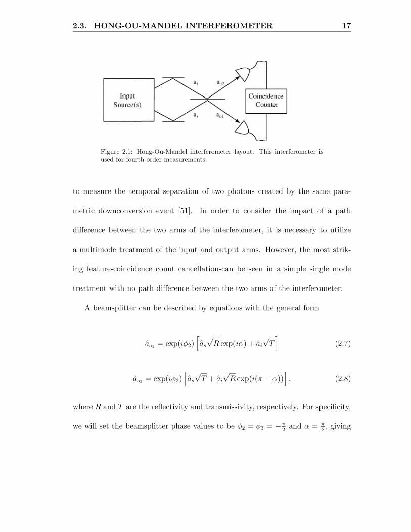
2.3. HONG-OU-MANDEL INTERFEROMETER 17
Figure 2.1: Hong-Ou-Mandel interferometer layout. This interferometer isused for fourth-order measurements.
to measure the temporal separation of two photons created by the same para-
metric downconversion event [51]. In order to consider the impact of a path
difference between the two arms of the interferometer, it is necessary to utilize
a multimode treatment of the input and output arms. However, the most strik-
ing feature-coincidence count cancellation-can be seen in a simple single mode
treatment with no path difference between the two arms of the interferometer.
A beamsplitter can be described by equations with the general form
ao1 = exp(iφ2)[as
√R exp(iα) + ai
√T
](2.7)
ao2 = exp(iφ3)[as
√T + ai
√R exp(i(π − α))
], (2.8)
where R and T are the reflectivity and transmissivity, respectively. For specificity,
we will set the beamsplitter phase values to be φ2 = φ3 = −π2 and α = π
2 , giving

2.3. HONG-OU-MANDEL INTERFEROMETER 18
the relationships [58]
ao1 =√
Ras − i√
T ai (2.9)
ao2 = −i√
T as +√
Rai. (2.10)
The count rate in one of the output arms is given by
〈a†o1
ao1〉 = R〈a†sas〉 + T 〈a†
i ai〉 + i√
RT [〈a†i as〉 − 〈a†
sai〉] (2.11)
and the coincidence count rate between the two detectors is given by
〈a†o1
a†o2
ao2 ao1〉 = RT 〈a†sa
†sasas〉 + R2〈a†
sa†i aias〉
+T 2〈a†i a
†sasai〉 + RT 〈a†
i a†i aiai〉
+2 RT 〈a†sa
†saiai〉 − 2 RT 〈a†
sa†i asai〉 (2.12)
The single detector count rate can thus be found to be
〈a†o1
ao1〉 =
1 for |11〉
|α0|2 for |α0α0〉(2.13)
where the relationship R + T = 1 has been used. We can see that in both cases
the result is nonzero and is independent of the specific values of the reflectivity
and transmissivity.

2.3. HONG-OU-MANDEL INTERFEROMETER 19
The coincidence count rate between the two detectors has the value for these
states of
〈a†o1
a†o2
ao2ao1〉 =
(R − T )2 for |11〉
|α0|4 for |α0α0〉(2.14)
We can see that in this case the specific value of the coincidence count rate can
depend on the value of the reflectivity and transmissivity. Furthermore, for the
50/50 beamsplitter of the HOMI, the coincidence count rate vanishes for two-
photon entangled state input. This absence of coincidence counts when the single
detector rates are nonzero is the signature of quantum interference in the HOMI.
This stands in contrast to the results for coherent state input, for which the
coincidence count rate simply equals the product of the single detector rates.
When the spectral distribution that is present in the interferometer source is
to be considered, a multimode analysis using a field description such as that in
Equation 1.2 is necessary. Using such a model, and assuming a Gaussian spectral
distribution, the coincidence count rate is found to have the form [51]
Rate ∝ R2 + T 2 − 2RTe−( ττc )
2
(2.15)
where τ is the time delay between the two arms and τc is the coherence time
between the downconverted photons. This coherence time is determined by the
width of the spectral distribution present in these two arms. The coincidence
count rate plotted as a function of time delay thus has a minimum when the arms

2.3. HONG-OU-MANDEL INTERFEROMETER 20
Figure 2.2: Hong-Ou-Mandel interferometer coincidence count rate. Thecount rate is plotted as a function of time delay between the two interfer-ometer arms. As the time delay increases, the interference-created reductionin coincidence rate disappears. The time delay is normalized to the photoncoherence time, which is the inverse of the spectral width.
are perfectly matched. For a 50/50 beamsplitter, the coincidence count rate at
this minimum vanishes. As the time delay increases the coincidence count rate
increases to its asymptotic value (Figure 2.2). The range of time over which this
feature occurs provides a measure of the coherence time between the input arms
of the interferometer. For a parametric downconversion source, this coherence
time is a measure of the temporal separation between the photons from a single
downconversion event. [51]
For type-I downconversion, the output spectral distribution is symmetric with
respect to the signal and idler frequencies. The signal and idler photons are thus

2.4. MACH-ZEHNDER INTERFEROMETER 21
indistinguishable. This condition produces the interference effect with the great-
est visibility. For type-II downconversion with a broadband pump, however, the
output spectra of the signal and idler photons can differ. This difference increases
the distinguishability of the photons, and this spectral distinguishability leads to
a loss of contrast in the interference pattern produced [52–54]. Visibility can be
restored through the use of spectral filtering [59,53] or source symmetrization [49].
2.4 Mach-Zehnder interferometer
The Mach-Zehnder interferometer is another fourth-order configuration that has
been explored using two-photon entangled state input [55,39,5,4,60,61]. As with
the second-order Mach-Zehnder, the input beams are combined with a beamsplit-
ter, directed along two arms that may differ in pathlength, and recombined using
a second beamsplitter. In the fourth-order interferometer, the output is detected
with a coincidence count detector placed across the two output ports of the second
beamsplitter (Figure 2.3).
The input and output modes of the Mach-Zehnder are related by
ao1 =12(1 − eiχ) as +
−i
2(1 + eiχ) ai (2.16)
ao2 =−i
2(1 + eiχ) as +
12(−1 + eiχ) ai (2.17)
where χ is the phase difference arising from the difference in pathlength between

2.4. MACH-ZEHNDER INTERFEROMETER 22
Figure 2.3: Mach-Zehnder interferometer layout. The coincidence counterdisplayed would be used for fourth-order interferometric measurements. Forsecond-order measurements, the output of a single photodetector would beused.
the two arms. Using these relationships, the probability of a photodetection at
one of the output ports is proportional to Γ(1,1)(r, r; t, t) ∝ 〈a†o1
ao1〉 which has the
value
〈a†o1
ao1〉 =12(1 − cosχ)〈a†
sas〉 +12(1 + cosχ)〈a†
i ai〉 (2.18)
+12sinχ[〈a†
sai〉 + 〈a†i as〉]. (2.19)
When a coherent state is sent into one input port with the other left empty
(|α00〉), the single detector count rate is proportional to
〈a†o1
ao1〉 =12|α0|2(1 − cosχ). (2.20)
This pattern has a visibility of one. For a two-photon entangled state, the single
detector count rate has the value
〈a†o1
ao1〉 = 1 (2.21)
2.4. MACH-ZEHNDER INTERFEROMETER 23
which is invariant under changes in χ. The single detector rate for the second
detector has the form 〈a†o2
ao2〉 = 12 |α0|2(1 + cosχ) for coherent state input, and
〈a†o2
ao2〉 = 1 for a two-photon entangled state. Using these values, we can see that
the accidental coincidence count rate for these states is
〈a†o1
ao1〉〈a†o2
ao2〉 =
1 for |11〉
14 |α0|4 sin2 χ for|α00〉
(2.22)
We can thus see that the coincidence rate naively expected from the second-order
results is χ-dependent in the case of coherent state input and χ-independent in
the case of two-photon entangled state input.
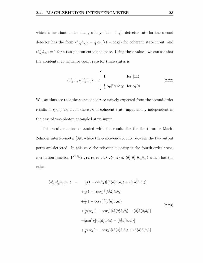
This result can be contrasted with the results for the fourth-order Mach-
Zehnder interferometer [39], where the coincidence counts between the two output
ports are detected. In this case the relevant quantity is the fourth-order cross-
correlation function Γ(2,2)(r1, r2, r2, r1; t1, t2, t2, t1) ∝ 〈a†o1
a†o2
ao2ao1〉 which has the
value
〈a†o1
a†o2
ao2ao1〉 = 14(1 − cos2χ)[〈a†
sa†sasas〉 + 〈a†
i a†i aiai〉]
+ 14(1 − cosχ)2〈a†
sa†i aias〉
+ 14(1 + cosχ)2〈a†
i a†sasai〉
+ 12sinχ(1 + cosχ)[〈a†
sa†sasai〉 − 〈a†
i a†saiai〉]
−12sin
2χ[〈a†sa
†saiai〉 + 〈a†
sa†i asai〉]
+ 12sinχ(1 − cosχ)[〈a†
sa†i aiai〉 + 〈a†
sa†saias〉]
(2.23)

2.4. MACH-ZEHNDER INTERFEROMETER 24
Figure 2.4: Mach-Zehnder interferometer single detector and joint detectionprobabilities. The probabilities are displayed as functions of the phase differ-ence between the two interferometer arms. The joint detection probability(solid line) is dependent on the phase difference even though the single de-tector probability (dashed line) is constant.
For the states considered above, the coincidence count rate (Figure 2.4) is then
found to be proportional to
〈a†o1
a†o2
ao2 ao1〉 =
14 |α0|4sin2χ for |α0 0〉
cos2χ for |11〉(2.24)
Both inputs produce a phase-dependent coincidence count rate. However, com-
parison to the accidental coincidence count rate 〈a†o1
ao1〉〈a†o2
ao2〉 shows that the
result with coherent state input is simply equal to the accidental rate, whereas the
two-photon entangled state result significantly differs from the naively expected
rate for that state.

2.5. QUANTUM LITHOGRAPHY 25
Figure 2.5: Quantum lithography configuration. The interferometric patternis detected via two-photon absorption rather than coincidence count detec-tion.
2.5 Quantum lithography
Two-photon states have been predicted to produce sub-Rayleigh-limit features in
configurations like that shown in Figure 2.5 [6]. In this arrangement, source
beams are sent into the input ports of a 50/50 beamsplitter, and the resulting
beams are then recombined at an angle 2θ onto a two-photon absorber. The
angular separation introduces an effective phase shift of 2kx sin θ between the two
outputs from the beamsplitter, where x is the transverse coordinate along the
observation plane. With conventional classical interferometric lithography, the
resulting pattern has a minimum fringe spacing of λ/2 which occurs at grazing
incidence (θ = π/2).
With an input of the form |1〉|1〉, the resulting pattern has a minimum fringe
spacing that is decreased below this classical limit by a factor of 2 [6]. Spontaneous
parametric downconversion has been proposed for use in this arrangement as a
source of two-photon entangled states. The resulting reduction in fringe spacing
can be seen in the following single-mode analysis.
2.5. QUANTUM LITHOGRAPHY 26
The relationship between the source beams and the beams directed onto the
two-photon absorber is given by
a1 =1√2
[as − iai] (2.25)
a2 =1√2
[−ias + ai] . (2.26)
The phase shift between these two beams as they recombine at a location with
transverse coordinate x can be written χ = 2kx sin θ, where θ is the angle between
the two beams. The field detected at this location can be represented with the
annihilation operator a3 where
a3 = a1 + eiχa2. (2.27)
In terms of the input modes to the beamsplitter this expression can be written
a3 =1√2
[(1 − ieiχ)as + (−i + eiχ)ai
]. (2.28)
To see the output generated by a two-photon entangled state input into the
beamsplitter, we can evaluate 〈a†3a
†3a3a3〉 using a state of the form |1〉s|1〉i. This
gives the result
〈a†3a
†3a3a3〉 = 2(1 + cos 2χ). (2.29)

2.5. QUANTUM LITHOGRAPHY 27
Figure 2.6: Quantum lithography output patterns produced by two-photonentangled state (solid line) and coherent state (dashed line) input fields. Thepatterns are shown as a function of χ = 2kx where x is the transverse coor-dinate in the observation plane and k is the wavevector of the writing beams.The pattern created with a two-photon entangled state input varies morerapidly with transverse position than the pattern created with the coherentstate input.
We can see that the total coincidence count rate will vary as 2χ = 4kx sin θ,
which is twice as rapid a dependence on χ as with standard classical techniques [6]
(Figure 2.6). This rapid dependence has been interpreted in the context of the
de Broglie wavelength of the photon pair, which is half the wavelength of the
individual photons [62,16,63].
This reduction in fringe spacing beyond the Rayleigh limit has been demon-
strated in principle in an experiment utilizing a beamsplitter and coincidence
count detector in place of the two-photon absorbing substrate [8]. The |2〉|0〉 +
|0〉|2〉 state that can be generated by a |1〉|1〉 state followed by a beamsplitter

2.5. QUANTUM LITHOGRAPHY 28
Figure 2.7: Quantum lithography in-principle realization. In-principle ob-servation of reduced fringe width using two-photon entangled states. Theentangled states are generated with a double slit placed after the paramet-ric downconverter used to generate the observed photons. The experimentalsetup uses a beamsplitter and coincidence count detector in place of a two-photon absorbing substrate.
was instead generated with a double-slit mask placed after a parametric down-
converter in such a manner that both of the downconverted photons exit through
the same slit. The predicted change in spacing was observed when the slits were
illuminated by the downconverter but not when the slits were illuminated by a
coherent state input (Figure 2.7).
Reductions in effective wavelength with a fourth-order interferometric exper-
iment have also been observed within the framework of de Broglie wavelength
measurement [62]. A wavepacket of m photons can be considered to have a de
Broglie wavelength of λ/m, where λ is the wavelength of the individual photons.
The entangled states considered above thus have a de Broglie wavelength half
that of the photons they contain. When used in a fourth-order interferometric
arrangement such as a beamsplitter and coincidence count detector placed af-
ter a double slit, the resulting pattern has a spacing consistent with the λ/2 de

2.6. CONCLUSION 29
Broglie wavelength as long as the spatial profile of the beam is of the appropriate
shape [62].
It should be noted that classical methods have also been proposed to achieve
a reduction in fringe spacing of this size [64]. However, the possible extension of
this method to 2m-photon entangled states, with the concomitant improvement
by a factor of 2m, makes quantum lithography an area of special interest.
2.6 Conclusion
In this chapter, we have reviewed results obtained with two-photon entangled
states in the Hong-Ou-Mandel interferometer, Mach-Zehnder interferometer, and
quantum lithography configurations. Two-photon entangled states used as inputs
to the Hong-Ou-Mandel interferometer exhibit a reduction in coincidence counts
below the level expected based on the single detector rates. In the Mach-Zehnder
interferometer, the coincidence count rate obtained with two-photon entangled
state input exhibits a variation with phase difference between the two arms of the
interferometer that is not present in the single-detector rates; this behavior can
be contrasted to that obtained with coherent state input, where the coincidence
rate simply equals the product of the single detector rates. Two-photon entangled
states in the quantum lithography configuration produce a pattern which varies
as λ/4 rather than the λ/2 variation produced by conventional classical interfer-
ometric lithography. In each case, two-photon entangled states produce results

2.6. CONCLUSION 30
that significantly differ from those produced with coherent state input. In the
next chapter, we will consider whether the interesting effects associated with two-
photon entangled states persist when the gain of the parametric downconversion
source used to produce these two-photon states is increased.

31
Chapter 3
High-Gain Contributions toFourth-Order Interferometric
Output
3.1 Introduction
The output of a vacuum-initiated parametric downconverter consists of a super-
position of states containing multiple photon pairs, with one member of each pair
emitted into the signal mode and the other into the idler mode. These states can
be written in the form |m〉s|m〉i. The two-photon entangled state experiments
described in the previous chapter are conducted at gain levels low enough that
the output can be considered to consist only of the vacuum and states containing
a single photon pair (i.e. |1〉s|1〉i). These experiments are typically conducted
under conditions with low count rates, with the rarity of photon creation events
ensuring that multiple pair states can be neglected.
In applications such as quantum lithography, these low count rates, combined

3.1. INTRODUCTION 32
with the low cross-section for two-photon absorption, are of practical concern.
While the correlation between the photons in an entangled pair may lead to
two-photon absorption rates that are linear in intensity [65,66], it is nevertheless
unclear whether low detection rates will be problematic in a practical context.
Raising gain levels, with the attendant production of additional photon pairs, is
a seemingly straightforward way of circumventing this problem, however it is also
to be expected that these additional photon pairs will alter the character of the
fourth-order interferometric effects.
In this chapter, the effect of these additional photon pairs on the patterns
produced by selected fourth-order interferometric arrangements is analyzed. We
begin by discussing the limitations presented by low-gain sources in certain exper-
imental configurations. The model used for describing the output of spontaneous
parametric downconversion in the high-gain limit is then outlined. The effect of
increased single-pass gain on the output of a Hong-Ou-Mandel interferometer is
presented, and the result generalized to any fourth-order four-port interferome-
ter. This model is then applied to the Mach-Zehnder and quantum lithography
configurations. The effect of increased gain in these situations is presented.
We find that in the Hong-Ou-Mandel and Mach-Zehnder arrangements the
presence of multiple photon pairs causes the disappearance of effects such as co-
incidence count cancellation, but that in the quantum lithography configuration
desirable effects are preserved even in the high-gain limit. These results are in-
3.2. PDC AS A MULTIPHOTON SOURCE 33
terpreted in the context of multiple photon pair contributions to interferometric
output.
3.2 Parametric downconversion as a multipho-
ton source
At low gain levels, spontaneous parametric downconversion is a source of individ-
ual pairs of entangled photons. In the simplest case, when only a single signal
and idler mode are being considered, this output can be written |1 >s |1 >i.
When gain is increased, multiple pairs may be generated, leading to an output
that is a superposition of states of the form |m >s |m >i. As the single pass gain
parameter is increased from low values where the mean photon number is much
less than one to the regime where there is a significant probability of states with
photon numbers much greater than one, the interferometric output is modified in
a continuous fashion from a biphoton-like result to one applicable when multiple
photons are present. The impact of this transition on important properties such
as interference visibility can then be determined.
A simple model for parametric downconversion can be used to investigate the
transition from single photon pairs to photon numbers >> 1 (Figure 3.1). The
interaction between the signal mode as and idler mode ai can be described by the

3.2. PDC AS A MULTIPHOTON SOURCE 34
Figure 3.1: Parametric downconversion. (a) The downconversion processcouples a single signal mode to a single idler mode. (b) The coefficients Uand V describe the interaction. The input may be initiated by seeding or byvacuum state input.

3.2. PDC AS A MULTIPHOTON SOURCE 35
interaction Hamiltonian
H = ~g[a†sa
†iv0 + h.c.] (3.1)
The corresponding equations of motion are
das
dt= −igv0a
†i (3.2)
dai
dt= −igv0a
†s (3.3)
and have the solutions
as = Uas0 + V a†i0 (3.4)
ai = Uai0 + V a†s0 (3.5)
where
U = cosh G (3.6)
V = −i exp(iθ) sinhG, (3.7)
G represents the gain of the process and is dependent on the pump amplitude and
the size of the material nonlinearity. This gain factor may be written as G = g|v0|t
where t is the interaction time, |v0| is the pump amplitude, and g is proportional
to χ(2) (Figure 3.1).

3.3. EFFECT OF INCREASED GAIN ON THEHONG-OU-MANDEL INTERFEROMETER 36
Figure 3.2: Layout of a Hong-Ou-Mandel interferometer.
3.3 Effect of increased gain on the Hong-Ou-
Mandel interferometer
Before considering the effect of increasing gain on the output of a generalized
fourth-order interferometer, we can consider the effect of increased gain on a well-
analyzed fourth-order phenomenon-the reduction of coincidence count levels in a
Hong-Ou-Mandel interferometer.
In the Hong-Ou-Mandel interferometer [51], source beams are directed into
the input ports of a 50/50 beamsplitter and a photon counting detector is placed
at each output (Fig. 3.2). When the low-gain output generated by spontaneous
parametric downconversion is used as an input, the rate of coincidence counts
drops to zero for equal pathlengths. If a pathlength difference between the two
input arms is introduced, the coincidence count rate becomes nonzero; as the
difference increases, the rate increases to its asymptotic value. We can look at
the absence or presence of coincidence counts in the equal path configuration as

3.3. EFFECT OF INCREASED GAIN ON THEHONG-OU-MANDEL INTERFEROMETER 37
gain is increased to monitor the impact of multiphoton states on fourth-order
interferometric effects.
The two beams from the parametric amplifier are directed into the two input
ports of the 50:50 beamsplitter shown in Figure 3.2, where they are combined.
Using the beamsplitter relationships
ao1 =1√2
[−as + iai] (3.8)
ao2 =1√2
[ias − ai] , (3.9)
the output fields are expressed as
ao1 =1√2
[(Uas0 + V a†
i0) − i(Uai0 + V a†s0)
](3.10)
and
ao2 =1√2
[−i(Uas0 + V a†
i0) + (Uai0 + V a†s0)
]. (3.11)
The coincidence count rate is given by 〈a†o1
a†o2
ao2ao1〉 and for a vacuum state input
to the material, becomes
〈0, 0|a†o1
a†o2
ao2ao1 |0, 0〉 = |V |4 (3.12)

3.3. EFFECT OF INCREASED GAIN ON THEHONG-OU-MANDEL INTERFEROMETER 38
Figure 3.3: Hong-Ou-Mandel interferometer coincidence count rate as a func-tion of gain. Joint detection probability (solid) at the beamsplitter outputports normalized to the single detector probability (dashed line) as a func-tion of source nonlinear interaction strength. The horizontal line indicatesthe joint detection probability normalized to the product of single detectionprobabilities.
This implies that the disappearance of the coincidence count rate is dependent on
the specific values of U and V and is not in general zero.
The coefficients U and V are given by Eqns. 4.3 and 4.4. From these quan-
tities, the coincidence count rate can be plotted as a function of the interaction
strength G as shown in Figure 3.3. We can see that the coincidence rate deviates
significantly from zero even at values of G where the mean output photon number
is approximately one.
Given a vacuum input, the output state arising from a parametric downcon-
verter can be written as the sum of states of the form |n, n〉 [18]. As the gain is
increased, the relative contribution of states with greater n also increases. The

3.4. MULTI-PAIR FOURTH-ORDER INTERFEROMETRY 39
presence of these states leads to a deviation of the coincidence count rate from its
value of 0 for |1, 1〉, as seen in Eq. 3.12. It is straightforward to show that a state
|ψ〉1 = |n, n〉 injected into two ports of a beamsplitter described by Eqns. 3.8 and
3.9 has a coincidence count rate at the output 〈a†o1
a†o2
ao2ao1〉 = 12n(n − 1). For
a |1, 1〉 input this quantity vanishes; if a |2,2〉 state is input into a beamsplitter,
the joint detection probability is no longer 0. This is also true for any n > 1. As
the nonlinear interaction strength is increased and more photons are produced,
components such as these will make nonnegligible contributions to the output
from the nonlinear material. Even at values of the single-pass gain where the
mean photon number is smaller than one, states such as |2, 2〉 are present; thus
the coincidence count rate only truly vanishes when the single-pass gain goes to
zero.
3.4 Multi-pair fourth-order interferometry
From the results in the previous section, we can see that the presence of additional
photon pairs in the input to a particular fourth-order interferometric configura-
tion led to the disappearance of a biphoton-related phenomenon. In this section,
a generalized four-port fourth-order interferometer with multiphoton input is con-
sidered, allowing a unified treatment of the HOMI, Mach-Zehnder, and quantum
lithography configurations. The following calculation separates interferometer-

3.4. MULTI-PAIR FOURTH-ORDER INTERFEROMETRY 40
dependent coefficients from input-state-dependent expectation values, showing
explicitly the origin of additional contributions arising from multiple pair states.
We begin by using the HOMI to identify the specific contributions introduced
by the presence of multiple pairs, examining in this case the output from a beam-
splitter with variable reflection and transmission properties. For a beamsplitter
describable by
ao1 =√
Ras − i√
T ai (3.13)
ao2 = −i√
T as +√
Rai, (3.14)
the coincidence count rate is given by
〈a†o1
a†o2
ao2ao1〉 = RT 〈a†sa
†sasas〉 + R2〈a†
sa†i aias〉
+T 2〈a†i a
†sasai〉 + RT 〈a†
i a†i aiai〉
+2 RT 〈a†sa
†saiai〉 − 2 RT 〈a†
sa†i asai〉.
(3.15)
From the first four terms in this expression we can identify the four paths by which
coincidence counts can be generated. These paths are shown in Figure 3.4. Paths
(b) and (c) are the only paths that are present when the input is a biphoton. Path
(b) corresponds to both input photons being reflected; path (c) corresponds to
both input photons being transmitted. Paths (a) and (d) are present if more than
one pair is present at the interferometer input. Path (a) arises when two photons
from the signal arm are detected at the output, while path (d) arises when two

3.4. MULTI-PAIR FOURTH-ORDER INTERFEROMETRY 41
Figure 3.4: Possible contributions to the Hong-Ou-Mandel interferometercoincidence count rate. Processes (b) and (c) are present at both low andhigh gain levels. Processes (a) and (d) are not present when there is only onephoton per mode.
3.4. MULTI-PAIR FOURTH-ORDER INTERFEROMETRY 42
photons from the idler arm are detected. In both cases one photon is reflected
while the other is transmitted. The remaining two terms in Equation 3.15 reflect
interference between different paths. For a |1, 1 > state, the first, fourth, and fifth
terms are zero, which is consistent with the identification of paths (a) and (d)
with terms present only if multiple pairs are at the input.
We can now analyze a generalized four-port interferometer. Such an interfer-
ometer can be described with the relationships
ao1
ao2
=
A B
C D
as
ai
(3.16)
where as and ai are the input signal and idler modes and ao1 and ao2 are output

3.4. MULTI-PAIR FOURTH-ORDER INTERFEROMETRY 43
modes. The joint detection probability is then given by
〈a†o1
a†o2
ao2 ao1〉 = |C|2|A|2〈a†sa
†sasas〉
+|D|2|A|2〈a†sa
†i aias〉
+|C|2|B|2〈a†i a
†sasai〉
+|D|2|B|2〈a†i a
†i aiai〉
+2 ReC∗A∗DA〈a†sa
†saias〉
+2 ReC∗A∗CB〈a†sa
†sasai〉
+2 ReC∗A∗DB〈a†sa
†saiai〉
+2 ReD∗A∗CB〈a†sa
†i asai〉
+2 ReD∗A∗DB〈a†sa
†i aiai〉
+2 ReC∗B∗DB〈a†i a
†saiai〉
(3.17)
By analogy with the HOMI calculation, we can identify the expectation values
present in the first four terms with the individual contributions of the four paths
shown in Figure 3.4. The four paths can be grouped into two types: single-input
paths, in which the detected photons arise from only one input arm, and dual-
input paths, in which both input arms contribute one photon. Paths (b) and (c)
are dual-input paths and differ only in the specific mapping of each input arm
onto the output arms. These paths are the only paths present when the input
is a biphoton. The single-input paths (a) and (d) are present when multiple-
photon inputs are used. These paths are not present with a biphoton input and,

3.4. MULTI-PAIR FOURTH-ORDER INTERFEROMETRY 44
when introduced by increasing gain, contribute to a degradation of visibility in the
Hong-Ou-Mandel configuration. The remaining six terms arise from interference
between each of these paths; for many input states most of these terms vanish.
This situation is summarized in Table 3.1, which shows the value of each of
the terms in Equation 3.17 for different input states. For states generated by
spontaneous parametric downconversion, all of the interference terms are zero
except for the term generated by the interference of the two paths in which one
signal and one idler photon are detected. Furthermore, for a biphoton input, the
first and fourth terms, corresponding to the single-input paths, are also zero as
they require at least two photons in the involved input arm. We can also note
that all of the terms are present if coherent state inputs are used. In the quantum
lithography configuration, we will see that the presence of these additional terms
with coherent state input leads to components with undesired wider fringe spacing.
In addition to the expectation values shown in Table 3.1, the value of the joint
detection probability is determined by the interferometer-dependent coefficients
that multiply each expectation value (e.g. |C|2|A|2 for 〈a†sa
†sasas〉). The values
of these coefficients for various interferometers are shown in Table 3.2. In the
case of an OPA, the “interferometer” is simply the direct mapping of the signal
to output 1 and the idler to output 2, that is, A = D = 1, B = C = 0, while for

3.4. MULTI-PAIR FOURTH-ORDER INTERFEROMETRY 45
Table 3.1: Coincidence count rate contributions (Eq. 3.17) forvarious input states. The diagrammatic representation for eachexpectation value is shown on the left. Here “|mm〉” designatesthe situation in which exactly m photons fall onto each input port,“|α0α0〉” the situation in which the same coherent state falls ontoeach input port, and “OPA” the situation in which the signaland idler beams from an optical parametric amplifier are used asinputs.

3.4. MULTI-PAIR FOURTH-ORDER INTERFEROMETRY 46
Table 3.2: Coincidence count rate coefficients for various inter-ferometers. For four different situations (listed at the top) thecoefficient of the quantum expectation value of each contribution(listed on the left along with its diagrammatic representation) toEq. 3.17 is given. OPA refers to the joint detection probability atthe output of an optical parametric amplifier, HOMI refers to thejoint detection probability at the output of a 50/50 beamsplitter,and QL refers to the two-photon absorption rate at the recordingplane in a quantum lithography configuration.

3.4. MULTI-PAIR FOURTH-ORDER INTERFEROMETRY 47
the HOMI, the transfer matrix elements are given by
A = D =1√2
(3.18)
B = C =−i√
2. (3.19)
In the case of a measurement made directly at the outputs of an optical para-
metric amplifier, Equation 3.17 reduces to 〈a†sa
†i aias〉, which is simply the joint
detection probability for the signal and idler modes. From Table 3.1, we can
see that, as expected, the joint detection rate from the parametric amplifier is
increased over the level produced by coherent state input. The second column in
Table 3.2 shows the Hong-Ou-Mandel interferometer coefficients. The negative
sign on the dual-input interference term reflects the phase relationship that allows
quantum interference to reduce the observed coincidence count rate. The single-
input interference term 〈a†sa
†saiai〉 is also nonzero; however this term is zero for
parametric amplifier outputs at both biphoton and high-gain levels. For coherent
state input this term is present and leads to a net coincidence rate that shows no
interference properties.
Using this framework to calculate the Hong-Ou-Mandel interferometer joint
detection probability gives
〈a†o1
a†o2
ao2 ao1〉 = 14 [〈a
†sa
†sasas〉 + 〈a†
sa†i aias〉 + 〈a†
i a†sasai〉 + 〈a†
i a†i aiai〉]
+ 12 [〈a
†sa
†saiai〉 − 〈a†
sa†i asai〉]
(3.20)

3.4. MULTI-PAIR FOURTH-ORDER INTERFEROMETRY 48
Figure 3.5: Single-input (solid line) and dual-input (dashed line) contribu-tions to the Hong-Ou-Mandel interferometer coincidence count rate. Thedual-input contribution vanishes at all values of the mean photon number.
with the following results for each of the states considered. For a biphoton input,
〈a†o1
a†o2
ao2ao1〉 = 0. For a Fock states in both signal and idler arms, the joint
detection probability is 12m(m − 1) and for a parametric amplifier the probability
is m2. Rewriting this last result using m = |V |2 returns the previously obtained
result of |V |4 (Eq. 3.12).
Figure 3.5 shows this result with the contributions of the single- and dual-input
terms displayed separately. The dual-input terms combine to give a net probabil-
ity of zero; these are the only terms present for a biphoton input, leading to the
coincidence count cancellation that is the hallmark of the Hong-Ou-Mandel inter-
ferometer. The single-input terms that become dominant as the photon number
increases lead to a joint detection probability of m2 for the parametric amplifier.
We can note that this has the same form as the probability for a coherent state

3.5. MULTI-PAIR MACH-ZEHNDER INTERFEROMETRY 49
input 〈a†o1
a†o2
ao2 ao1〉 = |α0|4 = m2, with both being equal to the product of the
single detector probabilities. Inspection of Tables 3.1 and 3.2 shows that this
apparent similarity arises through the contribution of different terms in each case.
3.5 Multi-pair Mach-Zehnder interferometry
The analysis of the Hong-Ou-Mandel interferometer in the earlier sections was
restricted to the case where the signal and idler beams are each emitted into a
single mode. Because variations in the frequency of the signal and idler photons are
not considered, the effect of a phase difference between the two paths in a HOMI
cannot be analyzed with this simple model and thus the effect of increased gain
on the interference pattern as a whole cannot be analyzed. In the Mach-Zehnder
configuration (Figure 2.3), however, the presence of an additional recombination
of the beams at the second beamsplitter allows us to analyze the visibility within
the constraints of this model.
In this section the generalized formalism of the previous section is applied to
the fourth-order Mach-Zehnder interferometer, which is described by the matrix
elements
A = −D =12(1 − eiχ) (3.21)
B = C =−i
2(1 + eiχ) (3.22)
3.5. MULTI-PAIR MACH-ZEHNDER INTERFEROMETRY 50
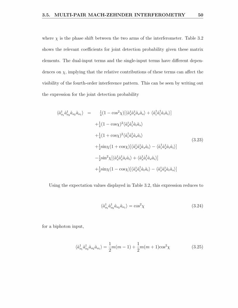
where χ is the phase shift between the two arms of the interferometer. Table 3.2
shows the relevant coefficients for joint detection probability given these matrix
elements. The dual-input terms and the single-input terms have different depen-
dences on χ, implying that the relative contributions of these terms can affect the
visibility of the fourth-order interference pattern. This can be seen by writing out
the expression for the joint detection probability
〈a†o1
a†o2
ao2 ao1〉 = 14(1 − cos2χ)[〈a†
sa†sasas〉 + 〈a†
i a†i aiai〉]
+14(1 − cosχ)2〈a†
sa†i aias〉
+14(1 + cosχ)2〈a†
i a†sasai〉
+12sinχ(1 + cosχ)[〈a†
sa†sasai〉 − 〈a†
i a†saiai〉]
−12sin
2χ[〈a†sa
†saiai〉 + 〈a†
sa†i asai〉]
+12sinχ(1 − cosχ)[〈a†
sa†i aiai〉 − 〈a†
sa†saias〉]
(3.23)
Using the expectation values displayed in Table 3.2, this expression reduces to
〈a†o1
a†o2
ao2 ao1〉 = cos2χ (3.24)
for a biphoton input,
〈a†o1
a†o2
ao2 ao1〉 =12m(m − 1) +
12m(m + 1)cos2χ (3.25)

3.5. MULTI-PAIR MACH-ZEHNDER INTERFEROMETRY 51
Figure 3.6: Mach-Zehnder fourth-order interference visibility for the para-metric amplifier as a function of source nonlinear interaction strength.
for a |mm〉 input, and
〈a†o1
a†o2
ao2 ao1〉 = m2 + m(m + 1)cos2χ (3.26)
for a parametric amplifier input. The corresponding visibilities are 1 for a bipho-
ton, (m + 1)/(3m − 1) for a |mm〉 state, and (m + 1)/(3m + 1) for a parametric
amplifier. As expected, the largest visibility occurs with a biphoton input. A
multiple pair input state has a visibility that decreases with increasing photon
number in each input mode. As expected, the parametric amplifier source has
visibility that is dependent on the mean photon number m, approaching unity for
low m and tending to 1/3 as m increases (Fig. 3.6).
A coherent state input leads to contributions from all terms, giving a joint de-

3.6. QUANTUM LITHOGRAPHY WITH MULTIPHOTON... 52
tection probability of 〈a†o1
a†o2
ao2ao1〉 = |α0|4cos2χ. This has the same dependence
on χ as that for a biphoton input and a visibility of 1. While the introduction of
single-input terms led to a decrease in visibility for high-gain parametric amplifier
input, the presence of additional terms in the coherent state case does not lead to
low visibility, but rather to a visibility of 1 even with large mean photon number.
3.6 Quantum lithography with multiple photon
pairs
In the HOMI configuration we have seen that the introduction of multiple pair
states as parametric amplifier gain is increased leads to fourth-order interfero-
metric output that resembles that produced by coherent state input. With the
fourth-order Mach-Zehnder interferometer, the introduction of multiple pair states
lead to a result with a visibility that not only is lower than that obtained with
biphoton input, but also lower than that obtained with coherent state input. In
the context of quantum lithography (Fig. 2.5), we will see that although increased
gain leads to a degradation in visibility relative to that obtained with biphoton
input, the desirable sub-Rayleigh pattern characteristics are preserved with multi-
ple pair states and are not preserved with coherent state input [67]. In particular,
while the interplay of the interferometer coefficients and the states’ expectation
values lead to similar results with coherent and parametric amplifier inputs for

3.6. QUANTUM LITHOGRAPHY WITH MULTIPHOTON... 53
the HOMI, the different weightings for each state present in the quantum lithog-
raphy case lead to qualitatively different results for the parametric amplifier and
coherent output states, even at high gain.
The matrix elements for quantum lithography are given by
A = C =1√2
−i√2eiχ (3.27)
B = D =−i√
2+
1√2eiχ (3.28)
where χ is proportional to the transverse coordinate across the substrate. It
should be noted that in the quantum lithography configuration, the joint detection
probability is related to the dose rate at a two-photon absorbing substrate rather
than to a traditional coincidence count detection system. Note also that since
the two outputs of the beamsplitter are combined on the lithographic plate, the
relevant field modes ao1 and ao2 of the general theory are identical in this case,
i.e. ao1 = ao2 . The quantum lithography coefficients, shown in the last column of
Table 3.2, are all non-zero and phase dependent. Thus states with different dual-
and single-input contributions can have net dose patterns that vary in spatial
frequency as well as overall magnitude.
The joint detection probability for the quantum lithography configuration is

3.6. QUANTUM LITHOGRAPHY WITH MULTIPHOTON... 54
given by
〈a†o1
a†o2
ao2ao1〉 = (1 + sin2χ)[〈a†sa
†sasas〉 + 〈a†
i a†i aiai〉]
+(1 − sin2χ)[〈a†sa
†i aias〉 + 〈a†
i a†sasai〉 + 2〈a†
sa†saiai〉 + 2〈a†
sa†i asai〉]
+2 sinχ[〈a†sa
†sasas〉 − 〈a†
i a†i aiai〉]
+2 cosχ[〈a†sa
†saias〉 + 〈a†
sa†sasai〉 + 〈a†
sa†i aiai〉 + 〈a†
i a†saiai〉]
+2 sinχ cosχ[〈a†sa
†saias〉 + 〈a†
sa†sasai〉 − 〈a†
sa†i aiai〉 − 〈a†
i a†saiai〉]
(3.29)
and reduces to 〈a†o1
a†o2
ao2ao1〉 = 4(1 − sin2χ) for a biphoton input, (1 +
sin2χ)[2m(m−1)]+(1− sin2χ)[4m2] for a |mm〉 input, and (1+sin2χ)[4m2]+(1−
sin2χ)[8m2 + 4m] for a parametric amplifier input, where the terms proportional
to 1 + sin2χ arise from the single-input paths and the 1 − sin2χ terms arise from
the dual-input paths. Figure 3.7 shows the parametric amplifier joint detection
probability, with the relative size of the single-input versus the dual-input contri-
bution plotted as a function of mean photon number. Recalling that the optimum
visibility of unity is achieved with a biphoton input which has no single-input con-
tribution, it can be seen that as the single-input contribution increases relative to
the dual-input contribution the visibility decreases to its limiting value of 1/5.
For each of the states generated by parametric downconversion, only terms
that oscillate at twice the phase difference are present. The absence of terms
oscillating as χ indicate that the patterns produced will have periods smaller than
the Rayleigh limit without undesired slower terms. This stands in contrast to the

3.7. CONCLUSION 55
Figure 3.7: Quantum lithography visibility as a function of mean photonnumber. The visibility decreases as the relative contribution of the single-input terms increases.
probability produced by coherent state inputs〈a†o1
a†o2
ao2 ao1〉 = {2(1 + sin2χ) +
6(1 − sin2χ) + 8cosχ}|α0|4. While the ”fast” sin2χ terms are present, the cosχ
term indicates the presence of undesired slower frequencies.
3.7 Conclusion
In this chapter, the results of calculations determining the effect of increased
source gain on the output of three fourth-order interferometric configurations are
presented. In these calculations, we have used a model of spontaneous parametric
downconversion in which a single signal mode and a single idler mode are coupled.
This model allows the gain to be varied in a continuous manner between the low-
and high-gain limits. Although the low-gain limit of this model approximates

3.7. CONCLUSION 56
a |11〉 state input, the presence of states such as |22〉 can cause the results to
deviate from the biphoton results even at low mean photon numbers. Because
of this, interferometer output patterns at high-gain are contrasted with both the
low-gain results and the results obtained with a pure |11〉 state.
A two-photon entangled state used as a source for a Hong-Ou-Mandel interfer-
ometer produces no coincidence counts when the arms are matched in pathlength,
even though the single detector rates are nonvanishing. The output obtained with
a spontaneous parametric downconverter deviated from this result at both low-
and high-gain levels. In general, the coincidence rate for the downconverter out-
put is equal to the product of the single detector rates, showing no coincidence
count cancellation even with equal arm pathlengths.
In a Mach-Zehnder interferometer, a two-photon entangled state source pro-
duces a fourth-order output proportional to cos2 χ, where χ is the phase difference
between the two arms; this pattern has a visibility of one. When an unseeded para-
metric amplifier is used, the pattern has the cos2 χ dependence of the entangled
state accompanied by an additional background term. The size of the background
relative to the phase-dependent component varies with gain level. As the gain is
lowered to zero, the visibility approaches one; in the high-gain limit, the visibility
decreases to the asymptotic value of 1/3.
In the third configuration, that of quantum lithography, a two-photon en-
tangled state produces a pattern that varies as cos2 χ where χ is the position-

3.7. CONCLUSION 57
dependent phase difference between the illuminating beams. This pattern has
the desired rapid dependence on χ as well as a visibility of one. An unseeded
parametric amplifier produces a pattern that also varies as cos2 χ but, as in the
Mach-Zehnder case, that is accompanied by a gain-dependent background term.
In the low-gain limit, the visibility approaches the two-photon entangled state
value of 1. As the gain is increased, the visibility is reduced to a value of 1/5.
The differences among the various results can be understood by decomposing
the expression for the joint detection probability of a generalized four-port fourth-
order interferometer into state-dependent and interferometer-dependent factors.
From this analysis, it can be seen that the loss of visibility arises from the presence
of coincidence counts due to photons from a single input arm. These single-input-
arm terms are not present in the two-photon entangled state case, where all coin-
cidences are attributable to pathways involving both input arms. Understanding
how to alter the relative amounts of each type of contribution by considering a
multimode analysis of these fourth-order interferometric systems is thus of inter-
est.

58
Chapter 4
Multimode Properties ofMulti-Pair Fourth-Order
Interferometry
4.1 Introduction
In the previous chapter, the transition from two-photon entangled states to in-
put states with multiple pairs was analyzed to see the effect of increased source
gain on the output of various fourth-order interferometric systems. In all of the
cases analyzed, the introduction of multiple photon pairs via increased gain led to
decreases in properties characteristic of the two-photon entangled state. In some
cases, desired properties such as coincidence count cancellation vanished entirely;
in others, the properties such as sub-Rayleigh spatial features were retained, but
with diminished visibility.
These analyses explored the origin of these differences by separating the effect
of the different interferometric configurations from the properties of the various
4.1. INTRODUCTION 59
input states considered. This framework allowed the identification of coincidence
rate contributions that occur only when multiple photon pairs are present and a
comparison of the role of these terms in different systems.
While these analyses outlined important features of the low-gain to high-gain
transition, they were restricted to the case where the signal and idler output
beams can be approximated as each consisting of a single mode. The analyses
thus could not encompass aspects of the photon source such as the distribution of
the output across different modes. In practice, these features of the light source
are also important determinants of the quantum properties visible in a particular
set-up.
In this chapter, we use a multimode treatment to compare the output of
fourth-order interferometric systems produced by two-photon and four-photon
input states. We again distinguish terms present only with multiple photon pairs
from terms present with two-photon states, analyzing the effect that the source
mode distribution has on the contribution of each of these terms.
We again find that the presence of these multiple photon pair terms in the high-
gain limit leads to significant differences in output from the two-photon case. We
find, however, that the mode selection properties of the interferometric system
can be used to influence the character of the output produced in the low- and
high-gain limits. In some cases, the effect of mode selection can be used to reduce
the effect of the multiple photon pair terms, suggesting that for certain systems

4.2. MULTIMODE SOURCE STATES 60
the degradative effect of increased gain can be mitigated by the appropriate ma-
nipulation of system properties.
We begin by presenting the model we will use to describe the unseeded para-
metric amplifier. We then use this model to calculate the output produced by
these states in a generalized four-port fourth-order interferometric system. The
differing effect of mode selection on the various terms contributing to two-photon
detection is described. These results are then applied to the Hong-Ou-Mandel
interferometer and quantum lithography configurations. The effects of a nonde-
generate mode distribution across the signal and idler on the multiple pair and
single pair output patterns as well as the interaction of mode selection with the
mode distribution on these output are presented.
4.2 Multimode source states
The output of a parametric downconverter consists of a superposition of states of
the form |m〉s|m〉i, where s and i designate the signal and idler modes. This can
be written |ψ〉 =∑
m ρ(m)|m〉s|m〉i, where the distribution ρ among these states is
dependent on the source gain. At low gain levels, this series is truncated after the
m = 0 and m = 1 terms; the parametric downconverter can thus be treated as a
two-photon source. As the gain increases, states consisting of multiple pairs such
as |2〉s|2〉i (four-photon) and |3〉s|3〉i (six-photon) become increasingly important,
requiring a model that includes these higher-order components.

4.2. MULTIMODE SOURCE STATES 61
In this section, we will begin by describing the multimode parametric amplifier
model used to analyze the effects of increased gain on the fourth-order interfero-
metric patterns generated by this type of source. It should be noted that the state
produced by a low-gain parametric amplifier is not formally equal to a biphoton
state due to the inclusion of higher-order terms. Thus, for reasons of comparison,
a multimode treatment of a biphoton state is also included.
4.2.1 Multimode parametric amplifier model
In Chapter 3, the signal and idler outputs of a parametric downconverter were
described using the single mode operators as and ai, related to the downconverter
input modes as0 and ai0 by relationships of the form
as = Uas0 + V a†i0 (4.1)
ai = Uai0 + V a†s0 (4.2)
where
U = cosh G (4.3)
V = −i exp(iθ) sinhG. (4.4)
The effect of increased gain was observed by increasing either the gain parameter
G or the mean single-arm photon number m = |V |2.

4.2. MULTIMODE SOURCE STATES 62
We now generalize this theory by allowing a distribution of signal and idler
modes to be present. We retain the assumption that a given idler mode is coupled
to one and only one signal mode, with the frequencies of these modes related by
ωs + ωi = ω0 where ωs, ωi, and ω0 are the frequencies of the signal, idler, and
pump beam respectively.
The relationship between a signal mode at ω and an idler mode at ω0 − ω is
now dictated by the frequency-dependent coefficients
U(ω) = cosh G(ω) (4.5)
V (ω) = −i exp(iθ) sinh G(ω) (4.6)
where
as(ω) = U(ω)as0(ω) + V (ω)a†i0(ω0 − ω) (4.7)
ai(ω0 − ω) = U(ω)ai0(ω0 − ω) + V (ω)a†s0(ω). (4.8)
Note that the gain parameter G is now frequency-dependent, incorporating a
factor that is dependent on the specific distribution of gain across frequencies as
well as a factor that is dependent on the overall gain level as governed by quantities
such as the pump strength. The form of the distribution of frequencies that see
gain is dependent on the material and pump parameters.

4.2. MULTIMODE SOURCE STATES 63
For field operators of the general form
E(+)(r, t) =∫
dωN(ω)a(ω)ei(k(ω)·r−ωt), (4.9)
the single photon detection probability in the signal arm for an unseeded para-
metric amplifier can be shown to be given by
〈E(−)s (r, t)E(+)
s (r, t)〉 =∫
dω|N(ω)|2|V (ω)|2. (4.10)
The idler single detector probability for the unseeded case is similarly given by
〈E(−)i (r, t)E(+)
i (r, t)〉 =∫
dω|N(ω)|2|V (ω0 − ω)|2. (4.11)
As in the single-mode model used in Chapter 3, the quantity |V |2 is an indicator
of the number of photons created in each arm. In the unseeded case, this number
grows from zero.
We can see that if |V (ω)|2 is centered around a frequency ω0s , the signal beam
will have a distribution of frequencies centered around ω0s ; V (ω) can thus be re-
garded as a signal frequency distribution function. Furthermore, the correspond-
ing idler beam has a distribution of frequencies governed by |V (ω0 − ω)|2. This
distribution will be centered on ω0 − ω0s . The signal and idler distributions will
be degenerate if ω0s = ω0/2 and nondegenerate otherwise. If the distributions

4.2. MULTIMODE SOURCE STATES 64
are nondegenerate, the signal and idler distributions are centered around differ-
ent frequencies and thus may be distinguished to some degree by their spectral
content.
4.2.2 Two-photon entangled state
In general, the output state containing a single photon pair can be described
by [39]
|ψ1〉 =∫ ∫
dωsdωiφ(ωs, ωi)|ωs〉s|ωi〉i (4.12)
where, in the limit of perfect entanglement,
φ(ωs, ωi) = φ′(ωs)δ(ω0 − ωs − ωi) (4.13)
and, in the limit of no entanglement,
φ(ωs, ωi) = φ′(ωs)φ′′(ωi). (4.14)
For states generated by parametric downconversion, the degree of entangle-
ment is dependent on experimental parameters such as the length of the interac-
tion region (determined by the nonlinear crystal length), the beam width at the
crystal, and the spectral width of the input beam [28,68,29]. It is possible to have
ωs + ωi take on a range of values, depending on the value of the relevant physical

4.2. MULTIMODE SOURCE STATES 65
parameters. In this analysis, as in Section 4.2.1, the relationship ωs + ωi = ω0 is
assumed.
For a state of the form given in Equation 4.12, the normalization condition
〈ψ1|ψ1〉 = 1, requires that
∫ ∫dωsdωi|φ(ωs, ωi)|2 = 1 (4.15)
Note that the total output state is given by
|ψ〉 = ρ(0)|vac〉s|vac〉i + ρ(1)|ψ1〉. (4.16)
If
|ρ(0)|2 + |ρ(1)|2 = 1 (4.17)
and
〈ψ1|ψ1〉 = 1 (4.18)
the output state will be properly normalized.
We can now use these multimode models with a generalized fourth-order inter-
ferometer to compare the output produced by an unseeded parametric amplifier
operated at both low- and high-gain with the output produced by a two-photon
4.3. GENERALIZED MULTIMODE FOURTH-ORDERINTERFEROMETER 66
entangled state. The multimode nature of these models allows us to examine the
effect of the interferometer characteristics on the output patterns generated. This
generalized description will then be interpreted in the context of the Hong-Ou-
Mandel interferometer and quantum lithography configurations.
4.3 Generalized multimode fourth-order inter-
ferometer
We assume field operators of the form given in Equation 4.9 and interferometer
input-output relationships of the form
ao1(ω)
ao2(ω)
=
A(ω) B(ω)
C(ω) D(ω)
as(ω)
ai(ω)
(4.19)
where as and ai are the input signal and idler modes and ao1 and ao2 are the
output modes. We can note that these are the same input-output relationships
used in Chapter 3, with the additional specification of the frequency dependence
associated with each operator.
If in addition we assume spectral filters in each arm f1(ω) and f2(ω), the
interferometer output field operators can be written
E(+)1 (r, t) =
∫dωN(ω)f1(ω)ao1(ω)ei(k(ω)·r−ωt) (4.20)

4.3. GENERALIZED MULTIMODE FOURTH-ORDERINTERFEROMETER 67
where ao1(ω) = A(ω)as(ω) + B(ω)ai(ω) and
E(+)2 (r, t) =
∫d3kN(ω)f2(ω)ao2(ω)ei(k(ω)·r−ωt) (4.21)
where ao2(ω) = C(ω)as(ω) + D(ω)ai(ω).
As discussed in Section 2.2 the instantaneous two-photon detection probability
density is given by the fourth-order correlation function
P (r1, t1; r2, t2) = Γ(2,2)(r1, r2, r2, r1; t1, t2, t2, t1) (4.22)
= 〈E(−)(r1, t1)E(−)(r2, t2)E(+)(r2, t2)E(+)(r1, t1)〉 (4.23)
where t1 and t2 are the times at which the output photons are detected. The
instantaneous probability can be integrated over the coincidence count resolution
time Tcr to give the coincidence count rate
R(r1, r2; t1) =∫ Tcr/2
−Tcr/2dτP (r1, t1; r2, t1 + τ ) (4.24)
This can in turn be integrated over the detector resolution time Td to give the
coincidence count probability for a given set of temporal parameters
P12(r1, r2) =∫ Td
−Td/2dtR(r1, r2; t) (4.25)
=∫ Td/2
−Td/2dt1
∫ Tcr/2
−Tcr/2dτP (r1, t1; r2, t1 + τ ) (4.26)

4.3. GENERALIZED MULTIMODE FOURTH-ORDERINTERFEROMETER 68
=∫ Td/2
−Td/2dt1
∫ Tcr/2
−Tcr/2dτ
× 〈E(−)(r1, t1)E(−)(r2, t1 + τ)E(+)(r2, t1 + τ )E(+)(r1, t1)〉.(4.27)
From Equations 4.20, 4.21 and 4.24 we can see that, as in Chapter 3, the
coincidence count rate will be dependent on both the interferometer coefficients A,
B, C, and D and state-dependent expectation values of the form 〈a†a†aa〉. Because
these expectation values are assessed in terms of operators at the interferometer
input, they can be calculated for the interferometer source independent of the
specifics of the interferometer used.
4.3.1 Expectation values at the source output
We can now used the states defined in Section 4.2 to calculate the expectation
values at the interferometer input. These values are dependent only on the source
characteristics.
Parametric amplifier
The expectation values describing the output of an unseeded parametric amplifier
can be calculated using Equations 4.7 and 4.8 together with a source input state
of the form |vac〉s|vac〉i where |vac〉 now represents a multimode vacuum state. As
in the single-mode case presented in Chapter 3 terms such as 〈a†sa
†i asas〉 vanish.

4.3. GENERALIZED MULTIMODE FOURTH-ORDERINTERFEROMETER 69
The nonzero terms are:
〈a†s(ω
′′′)a†s(ω
′′)as(ω′)as(ω)〉 =
V ∗(ω′′′)V ∗(ω′′)V (ω′)V (ω)[δ(ω0 − ω′′)δ(ω0 − ω′′′)
+δ(ω0 − ω′′′)δ(ω0 − ω′′)], (4.28)
〈a†s(ω
′′′)a†i(ω
′′)ai(ω′)as(ω)〉 =
V ∗(ω′′′)U ∗(ω0 − ω′′)U(ω0 − ω′)V (ω)δ(ω0 − ω′′′ − ω′′)δ(ω0 − ω′ − ω)
+V ∗(ω′′′)V ∗(ω0 − ω′′)V (ω0 − ω′)V (ω)δ(ω0 − ω′′′)δ(ω0 − ω′′), (4.29)
〈a†i(ω
′′′)a†s(ω
′′)as(ω′)ai(ω)〉 =
V ∗(ω0 − ω′′′)U∗(ω′′)U(ω′)V (ω0 − ω)δ(ω0 − ω′′′ − ω′′)δ(ω0 − ω′ − ω)
+V ∗(ω0 − ω′′′)V ∗(ω′′)V (ω′)V (ω0 − ω)δ(ω0 − ω′′′)δ(ω0 − ω′′), (4.30)
〈a†i(ω
′′′)a†i(ω
′′)ai(ω′)ai(ω)〉 =
V ∗(ω0 − ω′′′)V ∗(ω0 − ω′′)V (ω0 − ω′)V (ω0 − ω)[δ(ω0 − ω′′)δ(ω0 − ω′′′)
+δ(ω0 − ω′′′)δ(ω0 − ω′′)], (4.31)
〈a†s(ω
′′′)a†i(ω
′′)as(ω′)ai(ω)〉 =
V ∗(ω′′′)U ∗(ω0 − ω′′)U(ω′)V (ω0 − ω)δ(ω0 − ω′′′ − ω′′)δ(ω0 − ω′ − ω)

4.3. GENERALIZED MULTIMODE FOURTH-ORDERINTERFEROMETER 70
+V ∗(ω′′′)V ∗(ω0 − ω′′)V (ω′)V (ω0 − ω)δ(ω0 − ω′′)δ(ω0 − ω′′′), (4.32)
and
〈a†i(ω
′′′)a†s(ω
′′)ai(ω′)as(ω)〉 =
V ∗(ω0 − ω′′′)U∗(ω′′)U(ω0 − ω′)V (ω)δ(ω0 − ω′′′ − ω′′)δ(ω0 − ω′ − ω)
+V ∗(ω0 − ω′′′)V ∗(ω′′)V (ω0 − ω′)V (ω)δ(ω0 − ω′′′)δ(ω0 − ω′′). (4.33)
Comparison to Table 3.1 shows that these quantities reduce to the previously cal-
culated expectation values in the limit that only one signal and one idler mode,
each with frequency ω0/2, are occupied. It can be noted that in the multimode
case, the different terms have different dependences on the various frequencies ω-
ω′′′. In particular, the arguments of the U and V terms differ in the 〈a†sa
†i aias〉 and
〈a†i a
†sasai〉 expressions as compared to the 〈a†
sa†i asai〉 and 〈a†
i a†saias〉 expressions.
Recalling that for the Hong-Ou-Mandel interferometer the former pair of expec-
tation values correspond to the paths wherein one signal and one idler photon are
either both reflected or both transmitted, and that the latter pair of expectation
values correspond to the interference between these paths, we can see that the
shape of the gain distribution (i.e. the dependence of U and V on ω) will de-
termine the degree to which path interference leads to a reduction in coincidence
counts. This is consistent with the results relating distinguishability and quantum
interference [36,52,59] in the two-photon entangled state case.

4.3. GENERALIZED MULTIMODE FOURTH-ORDERINTERFEROMETER 71
Two-photon entangled state
Using the general form of the two-photon quantum state (Eq. 4.12), the various
two-photon expectation values at the output of the source material can be calcu-
lated. Since asas|ψ1〉 and aiai|ψ1〉 can be shown to vanish, as would be expected
for a state with only one photon in the signal and idler modes, all expectation
values containing two annihilation operators acting on the same mode will also
vanish (e.g. 〈a†sa
†sasas〉 = 0). The remaining two-photon expectation values are
given by
〈a†s(ω
′′′)a†i(ω
′′)ai(ω′)as(ω)〉 =
φ∗(ω′′′)φ(ω)δ(ω0 − ω′′′ − ω′′)δ(ω0 − ω − ω′),
〈a†i(ω
′′′)a†s(ω
′′)as(ω′)ai(ω)〉 =
φ∗(ω0 − ω′′′)φ(ω0 − ω)δ(ω0 − ω′′′ − ω′′)δ(ω0 − ω − ω′),
〈a†s(ω
′′′)a†i(ω
′′)as(ω′)ai(ω)〉 =
φ∗(ω′′′)φ(ω0 − ω)δ(ω0 − ω′′′ − ω′′)δ(ω0 − ω − ω′), (4.34)
and
〈a†i(ω
′′′)a†s(ω
′′)ai(ω′)as(ω)〉 =

4.3. GENERALIZED MULTIMODE FOURTH-ORDERINTERFEROMETER 72
φ∗(ω0 − ω′′′)φ(ω)δ(ω0 − ω′′′ − ω′′)δ(ω0 − ω − ω′). (4.35)
As with the parametric amplifier values, in the single-mode limit these values re-
duce the previously calculated quantities shown in Table 3.1. As was discussed in
the parametric amplifier case, the different frequency dependencies of the path in-
terference terms 〈a†sa
†i asai〉 and 〈a†
i a†saias〉 as compared to the other terms suggest
that the degeneracy of the gain parameter as expressed in the U and V coefficients
will influence the interferometer output.
4.3.2 Coincidence count rates
The coincidence count rates for the generalized fourth-order interferometer can
then be calculated using Equation 4.24, which relates the coincidence count rate
and the instantaneous joint detection probability, and Equations 4.20- 4.23, which
relate the instantaneous joint detection probability to the interferometer-specific
coefficients A, B, C, and D and to the source-determined expectation values
calculated in Section 4.3.1.
With these expectation values, the joint detection probability density
〈E(−)1 (r1, t1)E
(−)2 (r2, t2)E
(+)2 (r2, t2)E
(+)1 (r1, t1)〉 can be calculated for the paramet-
ric amplifier and two-photon input states. If the interferometer coefficients are
independent of frequency, this quantity can be written as the sum of several terms
〈E(−)1 (r1, t1)E
(−)2 (r2, t2)E
(+)2 (r2, t2)E
(+)1 (r1, t1)〉 =

4.3. GENERALIZED MULTIMODE FOURTH-ORDERINTERFEROMETER 73
|C|2|A|2〈E(−)1 E
(−)2 E
(+)2 E
(+)1 〉ssss
+ |D|2|A|2〈E(−)1 E
(−)2 E
(+)2 E
(+)1 〉siis
+ |C|2|B|2〈E(−)1 E
(−)2 E
(+)2 E
(+)1 〉issi
+ |D|2|B|2〈E(−)1 E
(−)2 E
(+)2 E
(+)1 〉iiii
+ 2ReC∗A∗DA〈E(−)1 E
(−)2 E
(+)2 E
(+)1 〉ssis
+ 2ReC∗A∗CB〈E(−)1 E
(−)2 E
(+)2 E
(+)1 〉sssi
+ 2ReC∗A∗DB〈E(−)1 E
(−)2 E
(+)2 E
(+)1 〉ssii
+ 2ReD∗A∗CB〈E(−)1 E
(−)2 E
(+)2 E
(+)1 〉sisi
+ 2ReD∗A∗DB〈E(−)1 E
(−)2 E
(+)2 E
(+)1 〉siii
+ 2ReC∗B∗DB〈E(−)1 E
(−)2 E
(+)2 E
(+)1 〉isii (4.36)
where each term 〈E(−)1 E
(−)2 E
(+)2 E
(+)1 〉jklm is given by
〈E(−)1 E
(−)2 E
(+)2 E
(+)1 〉jklm =
∫ ∫ ∫ ∫dω′′′dω′′dω′dω N∗(ω′′′)N∗(ω′′)N(ω′)N(ω)
×f∗1 (ω′′′)f∗
2 (ω′′)f2(ω′)f1(ω)e−i(k′′′·r1−ω′′′t1)e−i(k′′·r2−ω′′t2)
×ei(k′·r2−ω′t2)ei(k·r1−ωt1)〈a†j(ω′′′)a†
k(ω′′)al(ω′)am(ω)〉. (4.37)
We can note that Equation 4.36 is analogous to Equation 3.17, which relates the
joint detection probability to the interferometer-dependent coefficients and the
source-dependent expectation values in the single-mode case. When the interfer-
4.3. GENERALIZED MULTIMODE FOURTH-ORDERINTERFEROMETER 74
ometer coefficients are independent of frequency, the effect of the choice of source
and of the specific interferometer configuration can be separated term by term into
different factors. Since we are interested in understanding the effect of changing
source parameters on the interferometer output, this assumption is useful and will
be retained.
Parametric amplifier
Insertion of the parametric amplifier expectation values from Section 4.3.1 gives
instantaneous joint detection probabilities of the form
〈E(−)1 E
(−)2 E
(+)2 E
(+)1 〉ssss =
∫ ∫dωdω′ |N(ω)|2|N(ω′)|2f ∗
1 (ω′)f∗2 (ω)f2(ω′)f1(ω)e−i(k′·r1−ω′t1)
×e−i(k·r2−ωt2)ei(k′·r2−ω′t2)ei(k·r1−ωt1)|V (ω)|2|V (ω′)|2
+∫ ∫
dωdω′|N(ω)|2|N(ω′)|2|f1(ω)|2|f2(ω′)|2|V (ω)|2. (4.38)
We can note that in the single-mode limit, the joint detection probability
〈E(−)1 E
(−)2 E
(+)2 E
(+)1 〉ssss is proportional to |V |4 evaluated at the mode frequency.
This is the same dependence on V that was obtained in Chapter 3 for 〈a†sa
†sasas〉.
We can also note that the two terms differ in their time dependence. The second
term in Equation 4.38 is independent of the specific values of t1 and t2, suggesting
that it reflects accidental coincidences unrelated to specific photon pair correla-

4.3. GENERALIZED MULTIMODE FOURTH-ORDERINTERFEROMETER 75
tions. The first term in Equation 4.38 contains time-dependent exponentials. This
term thus may be expected to relate to coincidences arising from the nature of
the parametric amplification process.
Carrying out the time integration in Equation 4.24 gives the total coincidence
count rate in terms of the interferometer coefficients and the coincidence rates
arising from the integration of the individual joint detection probability terms. In
similar fashion to Equation 4.36, this relationship can be expressed as
R12 = |C|2|A|2Rssss + |D|2|A|2Rsiis + |C|2|B|2Rissi + |D|2|B|2Riiii
+ 2Re [C∗A∗DARssis + C∗A∗CBRsssi + C∗A∗DBRssii
+ D∗A∗CBRsisi + D∗A∗DBRsiii + C∗B∗DBRisii] (4.39)
where
Rjklm =∫ Tcr/2
−Tcr/2dτ〈E(−)
1 E(−)2 E
(+)2 E
(+)1 〉jklm (4.40)
and τ = t2 − t1. Integration over the exponential time-dependent factors gives
terms such as Tcrsinc( (ω−ω′)Tcr
2π ). Since the coincidence count resolution time Tcr
is typically much longer than the inverse of the width of the spectral distribution,
the sinc function will vary much more rapidly than the remaining factors within
the frequency integrals, allowing us to treat it as a delta function in ω.
The nonzero coincidence count rate contributions for the parametric amplifier

4.3. GENERALIZED MULTIMODE FOURTH-ORDERINTERFEROMETER 76
are given by
Rssss = Tcr
[∫dω|N(ω)|2|f1(ω)|2|V (ω)|2
] [∫dω|N(ω)|2|f2(ω)|2|V (ω)|2
]
+∫
dω|N(ω)|4|f1(ω)|2|f2(ω)|2|V (ω)|4, (4.41)
Rsiis = Tcr
[∫dω|N(ω)|2|f1(ω)|2|V (ω)|2
] [∫dω|N(ω)|2|f2(ω)|2|V (ω0 − ω)|2
]
+∫
dω|N(ω)|2|N(ω0 − ω)|2|f1(ω)|2|f2(ω0 − ω)|2|U(ω)|2|V (ω)|2 (4.42)
Rissi = Tcr
[∫dω|N(ω)|2|f1(ω)|2|V (ω0 − ω)|2
] [∫dω|N(ω)|2|f2(ω)|2|V (ω)|2
]
+∫
dω|N(ω)|4|f1(ω)|2|f2(ω0 − ω)|2|U(ω0 − ω)|2|V (ω0 − ω)|2 (4.43)
Riiii = Tcr
[∫dω|N(ω)|2|f1(ω)|2|V (ω0 − ω)|2
] [∫dω|N(ω)|2|f2(ω)|2|V (ω0 − ω)|2
]
+∫
dω|N(ω)|4|f1(ω)|2|f2(ω)|2|V (ω0 − ω)|4 (4.44)
and
Rsisi =∫
dω|N(ω)|2|N(ω0 − ω)|2|f1(ω)|2|f2(ω0 − ω)|2V ∗(ω)U ∗(ω)U(ω0 − ω)V (ω0 − ω)
+∫
dω|N(ω)|4|f1(ω)|2|f2(ω)|2|V (ω)|2|V (ω0 − ω)|2. (4.45)

4.3. GENERALIZED MULTIMODE FOURTH-ORDERINTERFEROMETER 77
Terms proportional to Tcr arise from the time-independent part of the instanta-
neous joint detection probability (e.g. Equation 4.38 for the ssss contribution)
and reflect accidental coincidence counts. As such, this contribution to the rate is
dependent on the coincidence count resolution time. As this time increases, the
rate of accidentals increases. Terms in which Tcr is absent reflect contributions
to the coincidence count rate that are intrinsic to the parametric amplification
process. Because we have assumed that the coincidence count resolution time is
much longer than the coherence time of the process, the count rate in this case is
independent of the specific value of the resolution time, depending solely on the
distribution functions describing the amplification process.
Two-photon entangled state
Insertion of the expectation values from Section 4.3.1 gives instantaneous joint
detection probabilities of the form
〈E(−)1 E
(−)2 E
(+)2 E
(+)1 〉siis =
∫ ∫dωdω′′ N∗(ω0 − ω′′)N∗(ω′′)N(ω0 − ω)N(ω)f∗
1 (ω0 − ω′′)f∗2 (ω′′)f2(ω0 − ω)f1(ω)
×e−i(k(ω0−ω′′)·r1−(ω0−ω′′)t1)e−i(k′′·r2−ω′′t2)ei(k(ω0−ω)·r2−(ω0−ω)t2)ei(k·r1−ωt1)
×φ∗(ω0 − ω′′)φ(ω) (4.46)

4.4. HONG-OU-MANDEL INTERFEROMETER RESULTS 78
The integration over the resolution time can be carried out as in Section 4.3.2 to
give the coincidence count rates
Rsiis =∫
dω|N(ω)|2|N (ω0 − ω)|2|f1(ω)|2|f2(ω0 − ω)|2|φ(ω)|2 (4.47)
Rissi =∫
dω|N(ω)|2|N (ω0 − ω)|2|f1(ω)|2|f2(ω0 − ω)|2|φ(ω0 − ω)|2 (4.48)
and
Rsisi =∫
dω|N(ω)|2|N(ω0 − ω)|2|f1(ω)|2|f2(ω0 − ω)|2
×φ∗(ω)φ(ω0 − ω). (4.49)
4.4 Hong-Ou-Mandel interferometer results
We will first apply these results to the Hong-Ou-Mandel interferometer. In Chap-
ter 3 we treated the case where there is no pathlength difference across the arms
of the interferometer. However, we can recall from the two-photon entangled
state results reviewed in Chapter 2 that when the multimode nature of the signal
and idler parametric downconverter outputs are taken into account, the result-
ing coincidence count rate is dependent on the pathlength difference between
arms [51]. When the arms are matched in length, the coincidence count rate falls
to its minimum. When the pathlength difference increases, the rate increases to

4.4. HONG-OU-MANDEL INTERFEROMETER RESULTS 79
an asymptotic level, with the rapidity of the increase determined by the size of
pathlength-induced time delay relative to the inverse of the output distribution
bandwidth. We will retrieve this result from the expressions derived in Section 4.3
for the two-photon entangled state case, then extend this analysis to a parametric
amplifier source.
The relationship between the input and output modes of a Hong-Ou-Mandel
interferometer can be described by the coefficients
A(ω) = D∗(ω) =1√2e
iωτ2 (4.50)
B(ω) = −C∗(ω) =−i√
2e
−iωτ2 . (4.51)
where τ is the time delay caused by the pathlength difference between the inter-
ferometer arms [39]. Because these coefficients are now dependent on the mode
frequency ω, the individual 〈E(−)1 E
(−)2 E
(+)2 E
(+)1 〉jklm terms in the expression for the
joint detection probability density (Equation 4.36) may now contain the interfer-
ometer coefficients within the frequency integrals; individual expectation values
that were previously dependent solely on the source characteristics can now be
dependent on the interferometer parameters as well. Because, for the states un-
der consideration, most of the terms affected by this change vanish, the only term
actually affected by this change is the 〈E(−)1 E
(−)2 E
(+)2 E
(+)1 〉sisi term.

4.4. HONG-OU-MANDEL INTERFEROMETER RESULTS 80
4.4.1 Two-photon entangled state
The coincidence count rate R12 for the two-photon entangled state can be ob-
tained by evaluating Equations 4.47-4.49 for a specific spectral distribution. Equa-
tion 4.49, which is the term associated with interference between path amplitudes,
is now modified by pathlength-associated exponential factors to the expression
Rsisi =∫
dω|N(ω)|2|N(ω0 − ω)|2|f1(ω)|2|f2(ω0 − ω)|2ei(ω0−2ω)τ
2
×φ∗(ω)φ(ω0 − ω). (4.52)
Using a Gaussian signal distribution for φ(ω) [28], the coincidence count rate
is found to be
R12 =14
{1 − e
− ω0s−ω0
i2∆ω
2
e−(∆ωτ2 )2
}(4.53)
where ω0s is the center of the signal distribution, ω0
i = ω0 − ω0s is the center of the
idler distribution, and 2∆ω is the width of the distributions. Note that we have not
included the effect of filters f1 and f2, and we have assumed that the normalization
varies slowly with ω, removing it from the integrals. We can see that, as expected,
the coincidence count rate for the Hong-Ou-Mandel interferometer is dependent
on the pathlength difference between arms, decreasing with increasing pathlength,
and on the degree of asymmetry between the signal and idler spectral distributions.
If the distributions are degenerate (ω0s = ω0
i = ω0/2), then the count rate reaches

4.4. HONG-OU-MANDEL INTERFEROMETER RESULTS 81
a minimum of zero. If the distributions are nondegenerate, then the count rate
minimum becomes shallower, with the count rate at some nonzero value even for
equal pathlengths. This lack of complete coincidence count cancellation can be
attributed to the loss of indistinguishability between the signal and idler outputs
of the downconversion [52,59,53].
4.4.2 Parametric amplifier
We can now extend these results to the case where the input to the interferometer
is an unseeded parametric amplifier described by Equations 4.7 and 4.8. As in
Section 4.4.1, we will ignore the filter functions and normalization constants, fo-
cusing on the role of the distribution functions V (ω) and U(ω). It is convenient to
rewrite the equations for the various contributions to the coincidence rate (Equa-
tions 4.41- 4.45) in terms of the single detector joint detection probability densities
Js = 〈E(−)s (r, t)E(+)
s (r, t)〉 =∫
dω|V (ω)|2 (4.54)
and
Ji = 〈E(−)s (r, t)E(+)
s (r, t)〉 =∫
dω|V (ω0 − ω)|2 (4.55)

4.4. HONG-OU-MANDEL INTERFEROMETER RESULTS 82
giving
R12 =14
{∫dω|V (ω)|4 + TcrJ
2s
+∫
dω|U(ω)|2|V (ω)|2 + TcrJsJi
+∫
dω|U(ω0 − ω)|2|V (ω0 − ω)|2 + TcrJiJs
+∫
dω|V (ω0 − ω)|4 + TcrJ2i
−2Re[∫
dωV ∗(ω)U ∗(ω)U(ω0 − ω)V (ω0 − ω)ei(ω0−2ω)τ
+∫
dω|V (ω)|2|V (ω0 − ω)|2]}
(4.56)
We can note that the last term, which is attributable to the interference between
possible paths, is the only term dependent on the pathlength difference between
arms. This parallels the two-photon entangled state results in this configuration.
We can also note the presence of terms proportional to the product of single
detector joint detection probability densities. These can be viewed as the rate
contribution arising from accidental coincidences. As such, these contributions
will increase as the window allowed for coincidences increases.
Relating these results back to the results of Chapter 3, we can consider the
case of degenerate signal and idler distributions with zero pathlength difference
between arms. In this case, the functions |U(ω)| and |V (ω)| will be invariant under
a change of arguments from ω to ω0 − ω, and the coincidence count rate further
reduces to R12 = TcrJ2s . (Figure 4.1) Noting that Js is proportional to the number

4.4. HONG-OU-MANDEL INTERFEROMETER RESULTS 83
Figure 4.1: Hong-Ou-Mandel interferometer joint detection probability as afunction of the source gain parameter G. The displayed values have beennormalized to the joint detection probability at G = 1. The joint detectionprobability is equal to the square of the single detector probability Js.
of single detector counts in the signal (or idler) arm, we can see that this expression
parallels that obtained in the single-mode case (Equation 3.12), where the joint
detection probability was found to be equal to the mean number of photons in
one of the amplifier output arms. Comparison to the two-photon entangled state
results shows that in this interferometer, the presence of additional photon pairs
arising from increased parametric amplifier gain leads to qualitatively different
results in the two cases.

4.5. QUANTUM LITHOGRAPHY RESULTS 84
4.5 Quantum lithography results
We can next apply this model to quantum lithography, extending the results of
Section 3.6 to the multimode case. The relationship between the input and output
modes in the quantum lithography configuration is describable by the coefficients
A = C =1√2(1 − ieiχ) (4.57)
B = D =1√2(−i + eiχ) (4.58)
where χ is proportional to the transverse coordinate across the observation plane.
We can recall that terms in the output pattern that vary as χ have a minimum
spacing of λ/2, while terms that vary as 2χ (e.g. cos2 χ) will have a minimum
spacing of λ/4. We will assume that no spectral filters are used, thus all filter
functions are replaced by 1 as in the previous sections. Note that we are treating
the phase difference as frequency independent. The features of primary interest
are the presence of components rapidly varying with χ (i.e. varying as 2χ), the
absence of components slowly varying with χ (i.e. varying as χ), and the overall
pattern visibility.
4.5.1 Two-photon entangled state
When the quantum lithography coefficients are used in conjunction with the ex-
pressions for the individual two-photon entangled state coincidence rate contribu-

4.5. QUANTUM LITHOGRAPHY RESULTS 85
tions (Equations 4.47-4.49), we obtain
R12 = [cos2 χ]∫
dω{|ψ(ω)|2 + |ψ(ω0 − ω)|2 + 2Reψ∗(ω)ψ(ω0 − ω)
}. (4.59)
For degenerate parametric downconversion ψ(ω) = ψ(ω0 −ω) and the coincidence
count rate reduces to 4 cos2 χ. A comparison of the two-photon quantum lithog-
raphy probability with the two-photon Hong-Ou-Mandel probability (Eq. 4.53)
shows that there is a different relationship between coincidence count terms in
the two cases. In the Hong-Ou-Mandel case, if the signal and idler are indistin-
guishable, the negative sign in the expression for the coincidence count proba-
bility causes the net probability to go to zero; as the spectral distinguishability
increases, the interference pattern becomes shallower, ultimately vanishing. In the
quantum lithography arrangement, this phase relationship among components is
not present. There is a cos2 χ dependence regardless of spectral distinguishability.
We can see that the use of a two-photon entangled state source produces a pattern
with the three desired characteristics of rapid dependence on χ, absence of a cos χ
component, and unit visibility.
4.5.2 Parametric amplifier
With a parametric amplifier input, the output pattern produced in the quantum
lithography configuration is less robust to changes in source parameters. In spe-
cific, we will see that the presence of single-input terms such as Rssss that are not

4.5. QUANTUM LITHOGRAPHY RESULTS 86
present in the two-photon case leads to a reduction in visibility. Because these
terms are increasingly present as gain is increased, the output pattern visibility
is sensitive to the gain level. In addition, the presence of accidental coincidences,
which are also absent in the two-photon case, leads to degradation of the visibility.
Comparison of the general expressions for the terms contributing to the coin-
cidence count rate in the parametric amplifier (Eqs. 4.41- 4.45) and two-photon
entangled state cases (Eqs. 4.47- 4.49) shows that the Rssss and Riiii terms that
vanish in the latter case are significant when a parametric amplifier is used as
a source. As discussed in Section 3.4, these terms can be attributed to the case
where two photons from a single input arm are detected together. The Rssss
can be identified with the contribution originating entirely from the signal arm
and Riiii with the contribution originating entirely from the idler arm. These
single-input terms can be seen to have different functional dependences on the
amplifier coefficients U and V than the dual-input Rsiis, Rissi, and Rsisi terms.
The single-input terms are entirely dependent on V (ω) while the dual-input terms
are dependent on integrands that vary with both |V |4 and |U |2|V |2. Noting that
|V | is smaller than |U | at low values of the gain parameter G, we might expect
that the dual-input terms will be dominant at the low-gain limit; this can be seen
to be true in Figure 4.2, plotted for the degenerate case. As the gain increases,
the |U |2|V |2 and |V |4 terms are seen to approach each other in size, implying that
the dual- and single-input terms make similar contributions at the high-gain limit.

4.5. QUANTUM LITHOGRAPHY RESULTS 87
Figure 4.2: Ratio between single-input (Rssss) and dual input (Rsiis) con-tributions to the coincidence count rate. This ratio does not include termsarising from accidental coincidences. The Rssss term is attributable to countswhere both photons arise from the signal arm. It is not significant at verylow gain levels. The integrand of this term is proportional to |V (ω)|4. TheRsiis term is attributable to counts where one photon is contributed by eachinput arm. The integrand of this term is proportional to |U (ω)|2|V (ω)|2.|V (ω)|4.

4.5. QUANTUM LITHOGRAPHY RESULTS 88
We can see the influence of each of these terms in the expression for the
quantum lithography coincidence count rate
R12 = (1 + sinχ)2{∫
dω|V (ω)|4 + TcrJ2s
}
+(1 − sin2 χ){∫
dω|U(ω)|2|V (ω)|2 + TcrJsJi
}
+(1 − sin2 χ){∫
dω|U(ω0 − ω)|2|V (ω0 − ω)|2 + TcrJiJs
}
+(1 − sinχ)2{∫
dω|V (ω0 − ω)|4 + TcrJ2i
}
+2(1 − sin2 χ)Re[∫
dωV ∗(ω)U ∗(ω)U(ω0 − ω)V (ω0 − ω)
+∫
dω|V (ω)|2|V (ω0 − ω)|2]
. (4.60)
The single-input contributions, which lead to the (1+sin χ)2 and (1−sin χ)2 terms
in this expression, are dependent solely on |V | and will contribute to a pattern
that goes as 1+sin2 χ. The dual-input terms vary as 1− sin2 χ and are dependent
on both |U | and |V |. Because the dual- and single-input terms each contain a
sin2 χ component, the desired rapid dependence on χ will be present. However,
because these two contributions are out of phase with one another, as the gain
increases the balance between these two components will shift, leading to changes
in the output pattern (Figure 4.3).
For the degenerate case shown in this figure, the equalities
JV 4 =∫
dω|V (ω)|4 (4.61)

4.5. QUANTUM LITHOGRAPHY RESULTS 89
Figure 4.3: Quantum lithography coincidence count rate as a function ofphase difference at various values of the gain parameter G. The count rateshave been normalized to peak values of 1 to allow for comparison between thevarious curves. The contribution from accidental coincidences has been sub-tracted from these curves. A significant decrease in visibility with increasinggain can be noted.
=∫
dω|V (ω0 − ω)|4 (4.62)
=∫
dω|V (ω)|2|V (ω0 − ω)|2, (4.63)
JU2V 2 =∫
dω|U(ω)|2|V (ω)|2 (4.64)
=∫
dω|U(ω0 − ω)|2|V (ω0 − ω)|2 (4.65)
=∫
dωV ∗(ω)U ∗(ω)U(ω0 − ω)V (ω0 − ω), (4.66)
and
Js =∫
dω|V (ω)|2 (4.67)
=∫
dω|V (ω0 − ω)|2 (4.68)

4.5. QUANTUM LITHOGRAPHY RESULTS 90
= Ji (4.69)
can be used to simplify the expressions for the output pattern
R12 = 4{JV 4 + TcrJ2s + JU2V 2 cos2 χ} (4.70)
and the visibility
Vis =JU2V 2
2JV 4 + JU2V 2 + 2TcrJ 2s
. (4.71)
The variation of this visibility with the gain parameter G is displayed in Figure 4.4
for the case where the accidental counts from the terms proportional to Tcr have
been removed. We can see that even in the case where the accidental counts
are assumed to be removable, the visibility decreases with increasing gain. In the
asymptotic limit, the visibility reaches 1/3. This value is higher than the 1/5 value
obtained in the single-mode case because the accidental counts that are present
with both models have been removed.
In the case where a coincidence counter is used to measure this fourth-order
pattern, the estimation and removal of the counts proportional to the coincidence
window is feasible. However, in the case where the joint detection is performed
by a two-photon absorbing substrate, the ability to compensate for the acciden-
tal coincidence rate cannot be assumed. Inspection of the visibility expression

4.6. EFFECT OF MODE SELECTION ON VISIBILITY 91
Figure 4.4: Quantum lithography pattern visibility as a function of the gainparameter G. The contribution from accidental coincidences is not included.The asymptotic value of the visibility is 1/3.
(Eq. 4.71) shows that as the coincidence count window is increased the visibility
will be lowered. This can be seen in Figure 4.5, which displays the patterns ob-
tained when the accidental coincidences are removed (equivalent to setting Tcr to
zero) and when the accidental rate is assumed nonzero.
4.6 Effect of mode selection on visibility
One issue yet to be addressed in this chapter is the effect of filtering on the
output patterns generated by these interferometric arrangements. We can re-
turn to the general expressions for the various coincidence count contributions for
the parametric amplifier (Eqns. 4.41- 4.45), this time focusing on the functional

4.6. EFFECT OF MODE SELECTION ON VISIBILITY 92
Figure 4.5: Quantum lithography output patterns as a function of the phasedifference with and without the inclusion of accidental coincidences. Thecontribution of these coincidences was included by using a value for the co-incidence count resolution time that produced an accidental rate equal tothe dual-input rate. As might be expected, accidental coincidences degradevisibility.
dependence of these terms on the filter functions f1 and f2. We will term the
situation where the filters in each arm have the same central frequency the sym-
metric filter case and situations where the filters have different central values as
the asymmetric case.
Given a degenerate spectral distribution and symmetric filters, the filters sim-
ply act in conjunction with the distribution to determine the observed distribution
width. However, asymmetries in the spectral distribution and filter settings can
affect the various contributions differently, shifting the balance between the com-
ponents of the coincidence count rate and affecting the observed interferometer
output.
The influence of spectral asymmetry has been well analyzed in the case of two-
photon entangled states [36,52,59,54]. If the signal and idler distributions (in our

4.6. EFFECT OF MODE SELECTION ON VISIBILITY 93
notation, represented by φ(ω) and φ(ω0 − ω) respectively), are centered around
different frequencies, the contribution of the term attributable to interference
between paths (Rsisi) decreases, thus reducing the amount of coincidence count
cancellation observed.
This result would seem to suggest that spectral asymmetry could lead to dele-
terious effects in the quantum lithography configuration as well. However, inspec-
tion of the dependence of the various terms in the coincidence count rate on the
phase difference χ
R12 = (1 + sinχ)2Rssss + (1 − sin2 χ) {Rsiis + Rissi} + (1 − sin χ)2Riiii
+2(1 − sin2 χ)ReRsisi (4.72)
shows that if terms contributing to the (1 − sin2 χ) variation are strongly favored
at the expense of terms contributing to a (1 + sin2 χ) variation, or vice versa, the
visibility will improve. On the other hand, if the two types of terms are made
more equal, they will cancel each other out, leading to little variation with χ.
Comparison of the single detector rates when filters are included shows that
there are four types of integrals present, that vary in filter and distribution. These
can be written as
J1s =∫
dω|f1(ω)|2|V (ω)|2 (4.73)

4.6. EFFECT OF MODE SELECTION ON VISIBILITY 94
J1i =∫
dω|f1(ω)|2|V (ω0 − ω)|2 (4.74)
J2s =∫
dω|f2(ω)|2|V (ω)|2 (4.75)
J2i =∫
dω|f2(ω)|2|V (ω0 − ω)|2 (4.76)
and correspond to the joint detection probability densities obtained when the sig-
nal or idler beams are directed into detectors 1 or 2. If the distribution V (ω)
is centered around a frequency ω0s that is not equal to ω0/2, the idler distri-
bution V (ω0 − ω) will be centered around a frequency ω0i that is not equal
to ω0s . If f1 is centered around ω0
s and f2 is centered around ω0i , J1s and
J2i will be favored. Terms such as∫
dω|f1(ω)|2|f2(ω)|2|V (ω)|4 in Rssss and
∫dω|f1(ω)|2|f2(ω0 − ω)|2|U(ω)|2|V (ω)|2 in Rsiis (Eqns. 4.41- 4.45) will also be
affected, with the Rssss integral diminished while Rsiis is favored. As discussed
above, this type of differential effect will lead to a diminishment of the desired
effect in the Hong-Ou-Mandel interferometer configuration, but could lead to in-
creased visibility in the quantum lithography configuration. These results suggest
that filter selection in conjunction with an nondegenerate spectrum can shift the
balance among various coincidence count rate contributions, altering the output
pattern either favorably or unfavorably.

4.7. CONCLUSION 95
4.7 Conclusion
In this chapter we generalized the parametric amplifier model used in Chapter 3 to
the case where multiple signal and idler modes may be occupied. This multimode
model was then used to reanalyze the Hong-Ou-Mandel interferometer and quan-
tum lithography configurations. Throughout this chapter, the output produced
with two-photon entangled state input was used as a basis for comparison.
The feature of interest in the Hong-Ou-Mandel interferometer configuration
was the coincidence count reduction that occurs when the time delay between
the two interferometer arms is less than the inverse of the spectral distribution
bandwidth. We found that the expression for the coincidence count rate produced
by an unseeded parametric amplifier contained terms that could contribute to
coincidence count reduction as well as background terms that are not present
in the two-photon case. The background terms are proportional to products of
single detector probabilities, suggesting that they can be attributed to accidental
coincidences. These terms lead to a loss of contrast in the generated pattern, as
the minimum coincidence rate increases with increasing gain. In the degenerate
case, with equal pathlengths, the parametric amplifier result echoes the single-
mode result presented in Chapter 3; the coincidence rate is proportional to the
product of the single detector probabilities.
In the quantum lithography configuration, two-photon entangled state input
produces a pattern with a minimum spacing of λ/4 and a visibility of one. Multi-

4.7. CONCLUSION 96
mode parametric amplifier input was found to retain the desirable λ/4 variation.
However, the visibility was strongly influenced by the presence of both background
terms and terms arising from the coincident detection of two photons from the
same input arm. Both of these types of contributions are absent in the two-
photon case. The visibility was strongly dependent on gain level, vanishing in the
high-gain limit.
Although the results in both cases indicate a diminishment or disappearance
of the desired output pattern property in the high-gain limit, the multimode treat-
ment also makes explicit the possibility of adjusting the balance between various
terms to alter the total interferometer output. In the Hong-Ou-Mandel interfer-
ometer case, spectral asymmetry leads to a decrease in pattern visibility. In the
quantum lithography case, however, the differing relationships among coincidence
rate components suggests the possibility of altering the relative sizes of terms in
a way that leads to increased rather than decreased pattern visibility.

97
Chapter 5
Vacuum-Initiated Filamentationas a Source of Entangled States
5.1 Introduction
It has often been observed that as a laser beam is passed through a nonlinear
medium it breaks up into a large number of filaments. This filamentation process
is initiated by the presence of weak perturbations on the laser wavefront, [69,70]
which can grow by means of four-wave mixing processes [71] and become large
enough to disturb the overall propagation of the beam. The questions addressed in
this chapter are whether vacuum fluctuations, which are intrinsic to the beam, can
act as perturbations to initiate filamentation and whether the generated beams
can serve as sources of single- and multiple-pair entangled states.
We begin with a discussion of filamentation as a four-wave mixing process. The
initiation of this process by vacuum fluctuations is then discussed [72]. We show
that vacuum fluctuations of the electromagnetic field constitute a fundamental

5.2. FILAMENTATION AS FOUR-WAVE MIXING... 98
perturbation to the incident laser field, and that filamentation initiated by these
quantum fluctuations places a realistic upper limit on the laser intensity that can
be transmitted through a given nonlinear optical material without the occurrence
of beam breakup.
The quantum properties of the states produced by filamentation are then an-
alyzed and the suitability of filamentation as a source for fourth-order interferom-
etry is discussed.
5.2 Filamentation as a four-wave mixing process
Self-focusing can be considered from the perspective of the nonlinear index of
refraction. Viewing the nonlinearity as a change in the refractive index leads nat-
urally to a treatment of self-focusing as a lens-like effect and is entirely appropriate
for discussions of whole-beam self-focusing. However, another segment of research
in this area concerns multimode effects, where the input beam is observed to break
up into multiple beams. In this case, an analysis of self-focusing in terms of the
growth of perturbations on the input beam has more utility and leads to a view
of filamentation as a four-wave mixing process.
Early experiments in self-focusing found that beams could evolve into both
single and multiple filaments [73]. For example, in 1966 Townes and co-workers
published experimental observations of a Q-switched beam collapsing into a sin-
gle filament with a diameter as small as 50 microns [74] and also demonstrated

5.2. FILAMENTATION AS FOUR-WAVE MIXING... 99
Figure 5.1: Four-wave mixing amplifies weak waves (ωs,ωi) at the expense ofthe pump wave (ω0).
the collapse of a single beam into many small (few micron) filaments. [75] Chiao,
Kelley and Garmire [71] gave a physical explanation of the growth of the off-axis
modes in terms of stimulated light scattering. They showed that the nonlinear
index of refraction allows the coupling of a strong incident wave with weak waves
having different transverse wavevectors. The four-photon interaction of a photon
with wavevector k1 = k0 + q, a photon at k2 = k0 − q and two pump photons
with k = k0 can allow the two weak waves to see gain (Figure 5.1). This gain is
dependent on the fulfillment of a phase-matching relation involving the partici-
pating waves. (Fig. 5.2) Because of this condition, certain transverse wavevectors
will see more gain than others and will come to dominate the spatial evolution of
the total field.
The magnitude of the wavevector that will see the maximum gain was calcu-
lated using phase matching considerations. From Figure 5.2 we can see that the
z-component of k1 should equal k0 for optimum phase matching. This gives the
relationship√
k21 − q2 = k0 . We can then substitute in k1 and k0 taking into ac-

5.2. FILAMENTATION AS FOUR-WAVE MIXING... 100
Figure 5.2: Self-focusing as a form of forward four-wave mixing.
count the weak-wave retardation of k1. This gives the magnitude of the dominant
transverse wavevector to be
q =√
k21 − k2
0 (5.1)
=ω
c
√(n0 + 2n2I)2 − (n0 + n2I)2 (5.2)
=ω
c
√2n0n2I + 3n2
2I2 (5.3)
This can be approximated to first order in n2 to be q = k0√
2n2I/n0 . This picture
is consistent with the model of Bespalov and Talanov [76], which predicted the
existence of a dominant instability size Λ = (π/k)√
n0/2n2I. It emphasizes the
ability of the self-focusing process to allow small perturbations to have a large
effect on the overall beam evolution.
Experimental confirmation of this effect, by Carman, et al. [77] and others [69]
followed. Among the characteristic signatures of this process are the growth of
perturbations at a rate dependent on the spatial frequency of the perturbations
and conical emission in the far-field.

5.3. FILAMENTATION INITIATION BY QUANTUMFLUCTUATIONS 101
5.3 Filamentation initiation by quantum fluctu-
ations
Our theoretical formalism follows closely that of Bespalov and Talanov, [76] which
treats the filamentation process classically by considering the gain seen by a wave-
front perturbation on a strong, monochromatic pump beam propagating through
a Kerr material. Our treatment differs from theirs in that we consider the op-
tical field to be a quantum mechanical quantity. The quantum fluctuations of
such a field (i.e., vacuum fluctuations) are necessarily spectrally broad band. Our
model thus predicts that quantum-initiated filamentation differs from its classical
counterpart in that it is accompanied by a spectral broadening of the transmitted
laser field. Our model also differs from its classical counterpart in that it leads
to explicit predictions regarding the strength of the fluctuations that initiate the
filamentation process.
Consider the propagation of a laser beam through a Kerr material. We can
express the positive frequency part of the total field as
E(+)(r, t) =[ε0 + ε1(r, t)
]eiγ0zei(k0z−ωt). (5.4)
Here ε0 denotes the amplitude of the strong pump field, which we have treated
classically, and which we assume to have frequency ω0 and wavevector k0 + γ0,
where k0 = n0ω0/c is its linear contribution and γ0 = n2I0ω0/c is its nonlinear

5.3. FILAMENTATION INITIATION BY QUANTUMFLUCTUATIONS 102
contribution, with n2 = (12π2/n20c)χ
(3) and I0 = (n0c/2π)|ε0|2. The perturbation,
which we are treating as a quantum mechanical operator, is denoted ε1 and is
conveniently decomposed in terms of its frequency components ω and transverse
wavevector components q as
ε1(r, t) =∫
d2q
∫ ∞
0dωN(ω)a(q, ω; z)ei(q·r)ei(kz(ω)−k0)z−i(ω−ω0)t. (5.5)
The mode amplitudes are denoted by a(q, ω; z) and satisfy the usual commutation
relation[a(q, ω; z), a†(q′, ω′; z)
]= δ2(q − q′)δ(ω − ω′). We have also introduced
the mode normalization factor N(ω) =√
~ω2n2(ω)/4π2kz(ω)c2. Note that we are
assuming that the nonlinear response can be modeled adequately by a disper-
sionless third-order susceptibility. We are thus ignoring effects such as those of
population trapping, which under certain conditions can prevent the occurrence
of self focusing. [78] We assume that n0 is frequency independent; the validity of
this assumption is discussed below. We further assume that n2I0 ¿ n0. Note
that we have taken the input pump beam to be a perfect plane wave. We have
done so to make clear that the onset of filamentation stems from the presence of
vacuum fluctuations and not from other perturbations to the input profile. While
the introduction of a finite beam width would bring new transverse components
into play, the evolution of these components leads simply to diffraction and to
whole beam self-focusing and does not alter these conclusions in any significant
way.

5.3. FILAMENTATION INITIATION BY QUANTUMFLUCTUATIONS 103
We insert the field E(+)(r, t) into the wave equation
∇2E(+) − 1c2
∂2
∂t2E(+) =
4πc2
∂2
∂t2P (+) (5.6)
where P (+) is the sum of the linear and nonlinear (i.e., 3χ(3)E(−)E(+)E(+)) con-
tributions of the material polarization. We linearize this equation in the pertur-
bation, and we make the paraxial and slowly varying amplitude approximations.
The paraxial approximation can break down under conditions of catastrophic self
focusing, but the present calculation deals only with the initiation of the fila-
mentation process which can be treated adequately within the framework of the
paraxial approximation. [79,80] We thereby obtain the coupled equations which
describe the spatial evolution of the mode amplitudes
d
dza(q, ω; z) = C(q, ω)a(q, ω; z) + D(q, ω)
[e−i∆kza†(−q, 2ω0 − ω; z)
](5.7)
d
dz
[e−i∆kza†(−q, 2ω0 − ω; z)
]= F (q, ω)a(q, ω; z) + E(q, ω)
[e−i∆kza†(−q,2ω0 − ω; z)
](5.8)
The coefficients that appear in these equations are given by
C(q, ω) = − i
2(kz(ω) + γ0)
(q2 + (kz(ω) + γ0)2 − k2(ω) − 4k0γ0
(ω
ω0
)2)
(5.9)
D(q, ω) =iγ0k0
kz(ω) + γ0)
(ω
ω0
)2
(5.10)

5.3. FILAMENTATION INITIATION BY QUANTUMFLUCTUATIONS 104
Figure 5.3: Filamentation phase-matching diagram. Wavevector matchingdiagram describing the four-wave mixing process that leads to filamentation.
E(q, ω) = −i∆k(ω) − C(q, 2ω0 − ω) (5.11)
F (q, ω) = −D(q, 2ω0 − ω) (5.12)
where
∆k(ω) = kz(ω) + kz(2ω0 − ω) − 2k0. (5.13)
We solve Eqs. 5.7 and 5.8 to obtain
a(q, ω; z) = a(q, ω; 0)eg0z
{cosh g1z +
C − E
2g1sinh g1z
}
+ e−i∆kza†(−q, 2ω0 − ω; 0)eg0z
{D
sinh g1z
g1
}(5.14)
where g0 = (C + E)/2 and g1 =√
(C − E)2 + 4DF/2. Note that we have not
assumed that the angle between the wavevectors of the pump and the perturbation
is necessarily small. We can thus treat interactions, such as that illustrated in Fig.
5.3, which for |k2| ¿ |k1| can be nearly phase matched even for large angles θ2. We

5.3. FILAMENTATION INITIATION BY QUANTUMFLUCTUATIONS 105
are required to include interactions of this sort because the quantum fluctuations
that initiate the four-wave mixing process are spectrally broad band. Inspection
of the form of the coefficients C(q, ω) and E(q, ω) shows that the gain eigenvalue
g0(q, ω) is always imaginary, but that the other eigenvalue g1(q, ω) can be either
real or imaginary depending on the values of q and ω. When g1(q, ω) is real, the
mode amplitude undergoes nearly exponential growth.
We next consider the effects of the growth of the mode amplitudes on the
overall propagation of the optical beam. We calculate the total intensity of the
perturbation as
Ifilament =nc
2π〈ε†
1(r, t)ε1(r, t)〉 (5.15)
=nc
2π
∫ 2ω
0dω
∫
R
dq2πq|N|2|D|2 sinh2 g1z
g21
(5.16)
where we have assumed that at the input to the nonlinear medium the pertur-
bation is in the vacuum state and where R denotes integration only over those
transverse wavevectors for which g1(q, ω) is real. We have evaluated this integral
and find that for z ¿ γ−10 the result can be approximated by
Ifilament(z) = 0.051n0c
2π
[~ω0k
20
4πγ0
]e2γ0z (5.17)

5.3. FILAMENTATION INITIATION BY QUANTUMFLUCTUATIONS 106
Figure 5.4: Normalized laser intensity at filamentation threshold (i.e. thenonlinear phase shift Bth) versus the nonlinearity parameter for various laserwavelengths.
which indicates that vacuum fluctuations supply an effective input intensity of
Ivac0 = 0.051
n0c
2π~ω0k
20
4πγ0 (5.18)
Using Equation 5.17, we readily determine the filamentation threshold distance
zf , which we arbitrarily take to be the distance at which the filament intensity
reaches one-tenth of the input pump intensity I0, and which is given by
zf =1
2γ0ln
8π2
0.51~ω0k30n2c
(5.19)
This result is illustrated in Fig. 5.4, which shows how the dimensionless parameter

5.4. FILAMENTATION AS AN INTERFEROMETRIC... 107
Bth = γ0zf = n2I0zfω0/c, which can be interpreted as the nonlinear phase shift
experienced by the pump wave at the threshold for filamentation, depends on the
nonlinearity parameter n2/n0 for a variety of laser wavelengths. Note that typical
threshold phase shifts are in the range 5 to 15, comparable to those of stimulated
scattering processes.
As a specific example of the application of these results, let us consider the case
of a laser beam propagating through air, for which n2 = 5×10⁻¹⁹cm2/W. [81] For
the case of an input beam at a wavelength of 775 nm with intensity 1011W/cm2,
we find that the effective vacuum input intensity is 0.128 mW/cm2 and that the
filament intensity reaches one-tenth of the input intensity at a distance of 40 m.
This distance is comparable to those that have been used in high-intensity laser-
beam propagation experiments. [82] We note, for comparison, that a beam with a
diameter of 3 cm has a whole beam self-focusing [83,84] distance of about 67 m and
a Rayleigh range of about 2 km. Filamentation induced by vacuum fluctuations
is thus seen to impose a realistic limitation on the intensities and distances over
which a high-power beam can propagate.
5.4 Filamentation as an interferometric source
Of interest in the context of multiphoton entangled state sources is whether the
vacuum-initiated filamentation process can serve as a source of correlated pho-
ton pairs in the same manner as spontaneous parametric downconversion. For

5.4. FILAMENTATION AS AN INTERFEROMETRIC... 108
this reason, we will close this chapter with a brief assessment of the similarities
and differences between the two processes. For simplicity we will consider the
frequency-degenerate case in the remainder of this chapter.
In the degenerate case, where all fields are at ω0, the relationship between
modes (for those that see gain) is given by
a(q, z) = U(q, z)a0(q) + V (q, z)a†0(−q) (5.20)
where
U(q, z) = cosh Λz −ξ
ΛsinhΛz (5.21)
V (q, z) =iγ
Λsinh Λz. (5.22)
γ is the nonlinear wavevector component, and ξ and Λ are transverse-wavevector-
dependent quantities. By inspection, it can be seen that Λ serves as the gain
parameter.
This type of mode relationship is clearly reminiscent of the parametric down-
converter mode relationship given in Equations 4.7 and 4.8. Instead of coupling
pairs of modes with the frequency relationship ωs +ωi = ω0, filamentation couples
pairs of modes with the wavevector relationship q1 + q2 = 0. As in the case of
parametric downconversion with a broadband pump, for which ω0 can take on a
range of values, the transverse wavevector relationship is relaxed if the pump field

5.4. FILAMENTATION AS AN INTERFEROMETRIC... 109
has a range of q components (e.g. a focused beam). The coupling of annihilation
operators to creation operators in both cases reflects the possibility of spontaneous
initiation of the process via vacuum fluctuations.
The processes differ in the specifics of the energy conservation relationships
obeyed. Because filamentation is a four-wave mixing process, all four photons
can be degenerate in frequency. This relationship is unlike the parametric down-
conversion case, in which, if spectral indistinguishability is to be maintained, the
signal and idler have approximately twice the wavelength of the pump. In quan-
tum lithographic applications, where maintaining a short wavelength is desirable
from the perspective of spatial resolution, a process in which the created photons
are degenerate with the pump is desirable.
While the wavelength degeneracy of filamentation can be seen as advantageous
in the context of resolution limits, it raises another concern–how to distinguish
the seeded process from the spontaneous process. As will be discussed in Chap-
ter 6, seeding with a coherent state alters the nature of the process and, in the
context of quantum lithography, can lead to the presence of an undesirable spatial
frequency component. It is thus desirable to be able to distinguish the seeded and
spontaneous processes. In parametric downconversion, because of the wavelength
difference between the pump and the signal, accidental seeding of the process
by the pump is not a concern. In beam filamentation, spatial components intro-
duced by wavefront irregularities often serve to seed the four-wave mixing process.

5.5. CONCLUSION 110
Addressing this issue is necessary for beam filamentation to have utility in this
context. If the goals are reversed, however, so that the observation of vacuum-
induced filamentation is the aim rather than the generation of a sub-Rayleigh
pattern, one might imagine that the presence or absence of the additional spatial
frequencies added by coherent-state input might be of use as an indicator of the
presence of seeding in the process.
5.5 Conclusion
In this chapter we have considered an alternative spontaneous wave-mixing process
as a generator of correlated photon pairs. We showed that vacuum-induced beam
filamentation places a limit on the light intensity that can be propagated through
a nonlinear material and compared this process to parametric downconversion in
the context of fourth-order interferometric configurations.

111
Chapter 6
Comparison to OtherMultiphoton Sources
6.1 Introduction
The states produced by parametric downconversion have interesting and useful
quantum properties at both the low and high gain levels. We have presented
calculations showing that certain fourth-order interferometric properties identified
with two-photon state inputs are retained even when the source gain is increased.
In some cases, the desired property is reduced to an asymptotic level; in other
cases, the desired property is retained, but only under a restrictive set of source
and interferometer conditions.
For example, in the case of quantum lithography, a two-photon entangled state
input produces a pattern with a spatial period of λ/4, no components at λ/2,
and a visibility of 1. When the parametric downconverter interaction strength is
increased, the periodicity of the pattern is retained, but the visibility drops to 1/5.

6.1. INTRODUCTION 112
The rate of visibility loss can be slowed dramatically in some cases through the use
of filtering, as the filtering process favors one type of coincidence count pathway
over the other pathways. Although the selection of a particular pathway produces
beneficial results in the quantum lithography configuration, it also reduces or
eliminates the terms arising from interference between pathways. Since this path
interference is a hallmark of other interferometers such as the Hong-Ou-Mandel
interferometer, it is clear that this filtering process cannot be generalized to other
fourth-order configurations. Furthermore, visibility enhancement in the absence
of pathway interference suggests that states with the unique characteristics of the
those produced by downconversion may not be required to achieve the results of
quantum lithography.
A question that follows naturally from results of this type is whether the
outputs produced by a high-gain parametric downconversion source can be dupli-
cated by a coherent state source. Although two-photon entangled state sources
have been shown to be superior to coherent state sources for the generation of
many of these properties of interest, it is less clear that the results produced by
high-gain parametric downconversion retain this superiority.
A related question is the extent to which the presence of a seed affects the
character of the pattern produced by parametric downconversion at low and
high gain levels. We have considered so far only processes initiated by vacuum
fluctuations–spontaneous parametric downconversion and vacuum-initiated fila-

6.1. INTRODUCTION 113
mentation. However, in a particular experimental setting, a seeded configuration
may be easier to implement. It is thus of interest to consider whether the presence
of a seed degrades the interferometric properties of interest.
In this chapter, we return to the single mode model of Chapter 3 to investi-
gate coherent and seeded parametric amplifier source states as multiphoton pair
fourth-order interferometric sources. The systems considered are the Hong-Ou-
Mandel interferometer and quantum lithography configurations. In each system,
the output property of interest differs. The property characteristic of a two-photon
entangled state source in the Hong-Ou-Mandel setup is coincidence count cancel-
lation. We thus use the coincidence count rate relative to the product of the
individual detector count rates as the basis for comparison of high-gain optical
parametric generator performance to that obtained by the use of coherent state
inputs. In the quantum lithography configuration, the variation of the output
pattern on wavelength and the size of this variation relative to its background
are the properties of interest. We thus use the presence of a λ/4 spatial compo-
nent, the absence of a λ/2 component, and the pattern visibility as the bases for
comparison.
We first consider the impact of seeding in this model and examine the implica-
tion of these results for the use of filamentation as a fourth-order interferometric
source. We then consider coherent state inputs, both phase coherent and phase in-
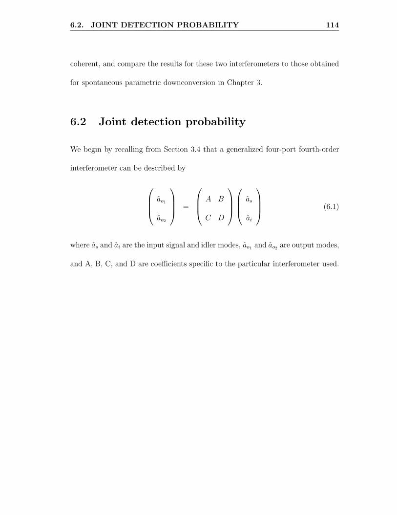
6.2. JOINT DETECTION PROBABILITY 114
coherent, and compare the results for these two interferometers to those obtained
for spontaneous parametric downconversion in Chapter 3.
6.2 Joint detection probability
We begin by recalling from Section 3.4 that a generalized four-port fourth-order
interferometer can be described by
ao1
ao2
=
A B
C D
as
ai
(6.1)
where as and ai are the input signal and idler modes, ao1 and ao2 are output modes,
and A, B, C, and D are coefficients specific to the particular interferometer used.

6.2. JOINT DETECTION PROBABILITY 115
The joint detection probability for this system is given by
〈a†o1
a†o2
ao2 ao1〉 = |C|2|A|2〈a†sa
†sasas〉
+|D|2|A|2〈a†sa
†i aias〉
+|C|2|B|2〈a†i a
†sasai〉
+|D|2|B|2〈a†i a
†i aiai〉
+2 ReC∗A∗DA〈a†sa
†saias〉
+2 ReC∗A∗CB〈a†sa
†sasai〉
+2 ReC∗A∗DB〈a†sa
†saiai〉
+2 ReD∗A∗CB〈a†sa
†i asai〉
+2 ReD∗A∗DB〈a†sa
†i aiai〉
+2 ReC∗B∗DB〈a†i a
†saiai〉.
(6.2)
We can again note that, proceeding term by term, the effect of the interferom-
eter and the effect of the choice of input state are separately described by co-
efficient products such as |C|2|A|2 and by fourth-order expectation values such
as 〈a†sa
†i aias〉. The overall impact of changing input states can thus be analyzed
through the comparison of the various signal and idler fourth-order expectation
values that appear in this equation. In Chapter 3 this comparison was conducted
for low- and high-gain output of an optical parametric generator; here we are con-
trasting the high-gain OPG output with a seeded parametric amplification process
and with various coherent state inputs.

6.3. SEEDED PARAMETRIC PROCESSES 116
6.3 Seeded parametric processes
In this section, we will calculate the output produced by a seeded parametric
process using the same model used in Section 3.4. The interaction between the
signal mode as and idler mode ai is described by
as = Uas0 + V a†i0 (6.3)
ai = Uai0 + V a†s0 (6.4)
where
U = cosh G (6.5)
V = −i exp(iθ) sinhG, (6.6)
G represents the gain of the process and is dependent on the pump amplitude and
the size of the material nonlinearity. For parametric downconversion, this gain
factor may be written as G = g|v0|t where t is the interaction time, |v0| is the
pump amplitude, and g is proportional to χ(2).
The spontaneous process and the seeded process are compared by using in-
put states at the entrance to the source material of |vac〉s|vac〉i and |α0〉s|vac〉i,
respectively. The various fourth-order signal and idler expectation values of Equa-

6.3. SEEDED PARAMETRIC PROCESSES 117
Table 6.1: Coincidence count rate contributions (Eq. 6.2) forstates produced by spontaneous and seeded parametric downcon-version. The diagrammatic representation for each expectationvalue is shown at left. Here |α0vac〉 designates an input stateseeded by a coherent state input. This state is compared to thatproduced by spontaneous parametric downconversion, designatedby |vac vac〉.
tion 6.2 can then be calculated for each choice of source seed state. The results
are shown in Table 6.1.
From Table 6.1, it can be seen that the fourth-order expectation values pro-
duced by the spontaneous and seeded processes are qualitatively quite different.
Several terms which vanish in the spontaneous case, such as 〈a†sa
†saias〉 are nonzero
in the seeded case. Furthermore, terms such as 〈a†sa
†sasas〉 and 〈a†
i a†i aiai〉 that were

6.3. SEEDED PARAMETRIC PROCESSES 118
equal in the spontaneous case have different values in the seeded case. These dif-
ferences may be expected to contribute to differences in interferometer output.
Applying these expectation values to the Hong-Ou-Mandel interferometer, it
can be shown that the joint detection probability is given by
〈a†o1
a†o2
ao2 ao1〉 =14
[(|U |4 + |V |4)|α0|4 + 4|V |2(|U |2 + |V |2)|α0|2 + 4|V |2
]
−12|U |2|V |2|α0|4 cos 4φ0, (6.7)
where a value of zero for the pump phase θ has been assumed. In the limit that
|α0| = 0, we regain the spontaneous result of |V |4 (Eq. 3.12).
The joint detection probability for the seeded process in the quantum lithog-
raphy configuration is given by
〈a†o1
a†o2
ao2 ao1〉 = (1 + sin2χ)[〈a†sa
†sasas〉 + 〈a†
i a†i aiai〉]
+(1 − sin2χ)2[〈a†sa
†i aias〉 + Re〈a†
sa†saiai〉 + Re〈a†
sa†i asai〉]
+2 sinχ[〈a†sa
†sasas〉 − 〈a†
i a†i aiai〉]
+4 cosχRe[〈a†sa
†saias〉 + 〈a†
sa†i aiai〉]
+4 sinχ cosχRe[〈a†sa
†saias〉 − 〈a†
sa†i aiai〉]
(6.8)
where the relationships 〈a†sa
†i aias〉 = 〈a†
i a†sasai〉 = 〈a†
sa†i aias〉 = 〈a†
sa†i asai〉,
〈a†sa
†saias〉 = 〈a†
sa†sasai〉, and 〈a†
sa†i aiai〉 = 〈a†
i a†saiai〉 have been used. This ex-

6.4. COHERENT STATE SOURCES 119
pression is very different from the expression for the spontaneous process
〈a†o1
a†o2
ao2ao1〉 = (1 + sin2χ)[4|V |4] + (1 − sin2χ)[8|V |4 + 4|V |2]. (6.9)
. We can note that terms that are absent in the spontaneous case, such as the
term proportional to sinχ, appear due to the imbalance between amplitudes such
as 〈a†sa
†sasas〉 and 〈a†
i a†i aiai〉. As these new terms are in general undesirable due
to their “slower” dependence on χ, the introduction of a seed can clearly have
detrimental effects. It is also important to note, however, that the size of these
effects is determined by the amplitude of the seed beam. Although the differences
between the two cases is qualitatively significant, if a weak seed beam is used, the
deviation from the spontaneous case may not be large and will clearly vanish as
the seed beam amplitude is decreased to zero.
6.4 Coherent state sources
We can next consider the patterns produced when coherent states are used as
inputs directly into the interferometer. Note that in this case, there are no signal
and idler beams in the conventional sense, rather “signal” and “idler” are simply
used to designate the two interferometer input modes as shown in Figure 3.4.
We will first consider two types of coherent state inputs–phase-coherent and
phase-incoherent–and will consider the effect of having matching (|α0〉s|α0〉i) or

6.4. COHERENT STATE SOURCES 120
Table 6.2: Coincidence count rate contributions (Eq. 6.2) for var-ious coherent state inputs. The diagrammatic representation foreach expectation value is shown at left. Here |α0α0 > and |α0α1 >designate input states with matching and unmatched amplitudes.The subscripts PCoh and PInc represent inputs that are phase co-herent and phase incoherent, respectively.
unmatched (|α0〉s|α1〉i) input amplitudes. As in the previous section, the various
states are compared by examining their fourth-order expectation values at the
input to the interferometer. Extending Table 3.1 to coherent state sources gives
Table 6.2, which displays the expectation value contributions to the joint detection
probability (Eq. 6.2) for states of this type. Comparison to Table 3.1 shows
that phase-incoherent coherent state inputs have expectation value contributions

6.4. COHERENT STATE SOURCES 121
similar to those determined for states of the form |mm〉 and∑
m |mm〉. All of the
states displayed have absent interference terms (last six terms listed), with the
exception of the term 〈a†sa
†i asai〉 and its complex conjugate. All of these states
also have 〈a†sa
†sasas〉, 〈a†
sa†i aias〉, 〈a†
i a†sasai〉, 〈a†
i a†i aiai〉 terms that are present, and
of equal or nearly equal magnitude.
Comparison with the coefficient list in Table 3.2 shows that the terms that dis-
tinguish the phase-coherent and phase-incoherent states (path interference terms
such as 〈a†sa
†saias〉) appear to be multiplied by coefficients that vanish in the case
of the Hong-Ou-Mandel interferometer, leading one to suspect that these two
types of coherent state inputs would produce the same Hong-Ou-Mandel joint
detection probability. However, closer inspection of the expression for this proba-
bility (Eq. 6.2) shows that the HOMI coefficients shown in Chapter 3 vanish only
because the expectation values for the states considered in that chapter are real.
Now that the expectation values can be complex (for the case of phase-coherent
|α0〉s|α1〉i input), the product of the coefficient and expectation value for a given
term must be calculated before the real part of the term is taken. Thus purely
imaginary HOMI coefficients like that for 〈a†sa
†saias〉 will combine with complex
expectation values such as |α0|3|α1|eiφ to produce nonzero contributions for terms
not present with OPG states. These considerations do not affect interferometer
coefficients such as those for quantum lithography that are entirely real. The in-

6.4. COHERENT STATE SOURCES 122
terferometer coefficients (Table 3.2) redone to show the full coefficient value are
shown in Table 6.3.
The interferometer-dependent coefficients combined with the state-dependent
expectation values can now be used with Equation 6.2 to calculate the joint detec-
tion probability for a particular configuration. Doing so for the Hong-Ou-Mandel
interferometer, with coefficients given by Eq. 3.18, gives
〈a†o1
a†o2
ao2ao1〉 =
14 [|α0|4 + |α1|4 + 2|α0|2|α1|2 cos 2φsi] for |α0α1〉PCoh
14 [|α0|4 + |α1|4] for |α0α1〉PInc
(6.10)
for inputs with different magnitudes. For inputs with that are matched in ampli-
tude, these expressions reduce to
〈a†o1
a†o2
ao2ao1〉 =
12 |α0|4[1 + cos 2φsi] for |α0α0〉PCoh
12 |α0|4 for |α0α0〉PInc
(6.11)
Note that the phase difference between the two input fields for the phase coherent
sources is designated φsi = φs − φi, and is applicable whether the inputs are of
equal or unequal magnitudes. (While we have used the notation |α0α0〉 for the
matched amplitude case, the calculations were conducted with an input state of
the form |α0〉s|α′0〉i where α0 = |α0|e−iφs and α′
0 = |α0|e−iφi .)
For a |α0〉s|α0〉i phase coherent input where there is no phase difference be-
tween the two input fields (φsi = 0), the joint detection probability 〈a†o1
a†o2
ao2 ao1〉
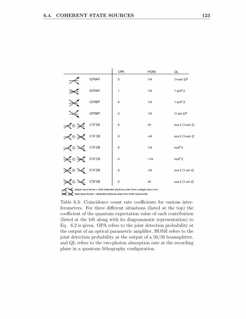
6.4. COHERENT STATE SOURCES 123
Table 6.3: Coincidence count rate coefficients for various inter-ferometers. For three different situations (listed at the top) thecoefficient of the quantum expectation value of each contribution(listed at the left along with its diagrammatic representation) toEq. 6.2 is given. OPA refers to the joint detection probability atthe output of an optical parametric amplifier, HOMI refers to thejoint detection probability at the output of a 50/50 beamsplitter,and QL refers to the two-photon absorption rate at the recordingplane in a quantum lithography configuration.

6.4. COHERENT STATE SOURCES 124
has the same value as the product of the two single detector probabilities 〈a†o1
ao1〉
and 〈a†o2
ao2〉. As was noted in Chapter 3, this is the same relationship that ex-
ists between the joint and single detection probabilities for the high-gain optical
parametric generator, for which 〈a†o1
a†o2
ao2 ao1〉 = 〈a†o1
ao1〉〈a†o2
ao2〉 = |V |4. Thus in
both cases there is no reduction in coincidence count rate below the level expected
from the single detector rates alone.
For |α0〉s|α0〉i phase coherent inputs that are π/2 out of phase (φsi = ±π/2),
the joint detection probability vanishes as it does for a two-photon entangled state.
However, examination of the single detector probabilities shows that this occurs
for the trivial reason that either 〈a†o1
ao1〉 or 〈a†o2
ao2〉 vanishes. This case is very
different from the |1〉s|1〉i state, for which the joint detection probability vanishes
although the single detector probabilities are nonzero.
The |α0〉s|α0〉i phase-incoherent result, which has the value 12 |α0|4 resembles
those obtained with |m〉s|m〉i states, which approach 12m
2 for large m. Compar-
ison between the phase-incoherent state expectation values in Table 6.2 and the
|m〉s|m〉i expectation values in Table 3.1 shows that the same terms are present
with both state types and that, in the limit of large m, all nonzero terms in both
cases have a value equal to the square of the single detector probability.
The results for quantum lithography follow a similar pattern, but have different
ramifications due to the different nature of the two interferometric arrangements.
With a low-gain parametric downconverter input (|1〉s|1〉i), the output pattern

6.4. COHERENT STATE SOURCES 125
has the desirable quality of unit visibility in a pattern that varies as λ/4 with no
“slow” λ/2 component. As the gain is increased, the visibility decreases to 1/5,
but the dependence on λ remains the same. We can compare these results to
the patterns obtained with coherent state input. For |α0〉s|α1〉iPCoh, the quantum
lithography output pattern is given by
〈a†o1
a†o2
ao2 ao1〉
= (1 + sin2 χ)[|α0|4 + |α1|4] + (1 − sin2 χ)2|α0|2|α1|2[2 + cos 2φsi]
+ 2 sinχ(|α0|2 − |α1|2) + 4 cos χ cos φsi|α0||α1|[(|α0|2 + |α1|2)
+ 4 sinχ cosχ cosφsi|α0||α1|(|α0|2 − |α1|2) (6.12)
and for |α0〉s|α1〉iPInc by
〈a†o1
a†o2
ao2 ao1〉 = (1 + sin2 χ)[|α0|4 + |α1|4] + (1 − sin2 χ)4|α0|2|α1|2
+2 sin χ(|α0|2 − |α1|2) (6.13)
where χ = 2kx is the phase difference between the beams incident on the obser-
vation plane at a transverse displacement x. In the limit that |α0| = |α1|, these
expressions reduce to
〈a†o1
a†o2
ao2 ao1〉
= (1 + sin2 χ)2|α0|4 + (1 − sin2 χ)2|α0|4[2 + cos 2φsi]

6.4. COHERENT STATE SOURCES 126
+ 8 cos χ cos φsi|α0|4 (6.14)
and
〈a†o1
a†o2
ao2ao1〉 = 2|α0|4(2 + cos2 χ) (6.15)
for |α0〉s|α0〉iPCoh and |α0〉s|α0〉iPInc, respectively.
From the case of phase-coherent |α0〉s|α0〉i input fields with no net phase
difference between them (φsi = 0), the joint detection probability reduces to
4|α0|4(2 − sin2 χ + 2 cos χ). We can note that this output pattern contain the
undesired cos χ component that varies as λ/2 and thus does not achieve a sub-
Rayleigh-limit pattern. If the cosχ term was simply ignored, the pattern resulting
from the remaining terms would have a visibility of 1/3. However, it is not possible
to adjust the phase difference between arms to eliminate the cosχ term without
also affecting the sin2 χ term, since the phase difference φsi is contained in both.
Choosing a value of φsi that eliminates the cos χ term, such as π/2, also leads the
sin2 χ term to vanish. We can note that this is unlike the output pattern produced
by the optical parametric generator at either low or high gain. The OPG pattern
contains no slowly varying cos χ or sinχ terms in either case.
The output pattern produced by phase-incoherent equal amplitude fields is
proportional to 3 − sin2 χ and thus does contain the desired 2χ variation without
a more slowly varying χ-dependent term. The remaining criterion for assessment

6.5. CONCLUSION 127
of this source is visibility. It can easily be shown that the visibility for this state
is 1/5, which is the same as that for a high-gain optical parametric generator.
6.5 Conclusion
In this chapter, the output of a high-gain optical parametric generator was com-
pared to a seeded parametric amplifier and various coherent states as sources for
various fourth-order interferometric systems. Section 6.3 showed that the intro-
duction of a seed qualitatively altered the quantum lithography output pattern,
adding undesirable components. The degree of deviation from the vacuum-seeded
pattern was dependent on the seed amplitude; a weak seed might be acceptable
depending on the size of the deviation that can be tolerated.
This result has implications for the utility of vacuum-induced beam filamenta-
tion as a source for fourth-order interferometric applications. While beam filamen-
tation and parametric downconversion can be treated with the same mathemati-
cal model, one significant difference is the presence of seeding for filamentation in
the form of wavefront aberrations. In parametric downconversion, the difference
between the wavelengths of the pump and the output beams allows the sponta-
neous process to be easily distinguished from the seeded process. In the case of
filamentation, the degeneracy in wavelength between the pump and the created
beams, while an advantage for resolution doubling, also implies that fluctuations
present on the pump wavefront can serve as seeds to the interaction; that seeded

6.5. CONCLUSION 128
process is not easily separated from the spontaneous process. The results of Sec-
tion 6.3 suggest that a small amount of seeding may still lead to acceptable results;
this, in turn, suggests that the issue of wavefront fluctuations need not prevent
vacuum-induced filamentation from being considered as a source for this type of
interferometric configuration.
Section 6.4 compared the fourth-order interferometric output of the high-gain
OPG to that produced by various coherent states. The results are summarized
in Table 6.4, which shows both the joint detection probability and the expected
coincidence probability defined as the product of the single detector probabilities.
This table also includes results calculated for the fourth-order Mach-Zehnder con-
figuration.
From this table we can see that, with an appropriate choice of phase relation-
ship between the two input beams, coherent state output can mimic the output
obtained with a two-photon entangled state at the level of the joint detection
probability alone. For instance, an output that varies with transverse coordinate
and wavelength (as contained in χ) in the same manner as that obtained with
a |11〉 can be achieved in the quantum lithography configuration with the use of
two randomly phased equal-amplitude coherent states. However, this apparent
similarity disappears when the values of the single detector rates are considered.
For both the Hong-Ou-Mandel and the Mach-Zehnder interferometers, the effect
of interest is difference between the calculated coincidence count rate and that

6.5. CONCLUSION 129
Table 6.4: Comparison of joint detection probabilities versusexpected coincidence levels. The expected coincidence level ishere defined as the product of the individual detector proba-bilities 〈a†
o1ao1〉〈a†
o2ao2〉 and is compared to the actual joint de-
tection probability 〈a†o1
a†o2
ao2ao1〉. The sources displayed are thetwo-photon entangled state (|11〉), the paired coherent state in-put (|α0α0〉), and the output of an optical parametric generator(OPG). The phases of the coherent state inputs were chosen tobest illustrate similarities in joint detection probabilities and dif-fer for each interferometer (φsi = π/2, HOMI; φsi = 0, Mach-Zehnder; random phase, QL).

6.5. CONCLUSION 130
expected based on the product of the single detector rates. In the case of coher-
ent state input, the calculated rate is simply the product of the single detector
rates, indicating no excess or reduction from the rate expected due to accidental
coincidences. In contrast, the two-photon entangled state produces a rate that
differs from the accidental rate, either in overall reduction as with the HOMI or
in dependence on phase difference between arms as in the Mach-Zehnder.
The high-gain optical parametric generator results vary by interferometer. In
the Hong-Ou-Mandel interferometer configuration, the calculated rate is the same
as the accidental rate. In the Mach-Zehnder, the calculated rate differs from the
accidental rate. Quantum lithography is unique among the three cases in that all
three sources show a deviation of the calculated coincidence rate from the acci-
dental coincidence rate. It is also unique in that the quantity of interest is truly
the joint detection rate alone, rather than the deviation of that rate from other
quantities. This implies that both high-gain OPG and coherent state sources
are of interest in this configuration. This conclusion is reinforced by the exis-
tence of classical proposals for the achievement of sub-Rayleigh-limit lithographic
sources [64]. In practice, details of substrate properties as well as the creation
of N-photon entangled sources will determine which configuration is of the most
experimental relevance.

131
Chapter 7
Conclusions
In this thesis, our focus has been the assessment of the utility of high-gain
sources such as unseeded parametric amplifiers in configurations conventionally
associated with two-photon entangled state sources. We have done so by using
a single-mode analysis to compare the outputs of three fourth-order interferome-
ters obtained with parametric amplifier and two-photon entangled state sources.
These analyses were extended to the multimode case in order to examine the
effect of system transfer characteristics on the results. Vacuum-induced beam
filamentation was then considered as an alternative to spontaneous parametric
downconversion as a source for fourth-order interferometric configurations. The
high-gain unseeded parametric amplifier results were then compared with the re-
sults obtained using coherent state and seeded amplifier sources.
The first set of analyses involved a model of parametric downconversion in
which a single signal mode was coupled to a single idler mode. The output of this
source was then used as an input to three different fourth-order interferometric

132
arrangements. The first interferometer considered was the Hong-Ou-Mandel in-
terferometer. We can recall that a two-photon entangled state used as a source for
this interferometer produces no coincidence counts when the arms are matched
in pathlength, even though the single detector rates are nonvanishing. We found
that the output obtained with a spontaneous parametric downconverter deviated
from this result at both low- and high-gain levels, and, in fact, that the coinci-
dence rate for the downconverter output was equal to the product of the single
detector rates. There was no coincidence count cancellation even with equal arm
pathlengths.
The second single-mode analysis considered the effect of different sources on
the output of a fourth-order Mach-Zehnder interferometer. With this interferom-
eter, a two-photon entangled state source produces a fourth-order output propor-
tional to cos2 χ, where χ is the phase difference between the two arms. This result
is notable given the independence of the single detector rates from χ. When an
unseeded parametric amplifier was used, the pattern was found to have the cos2 χ
dependence of the entangled state accompanied by an additional gain-dependent
background term. In the low-gain limit the visibility was found to increase to the
value of unity obtained with a two-photon entangled state source; in the high-gain
limit, the visibility was found to decrease to the asymptotic value of 1/3.
In the third configuration, that of quantum lithography, the most salient prop-
erties of the two-photon entangled state pattern are its visibility of one and its

133
lack of a slowly varying cosine dependence on kx. We show that the unseeded
parametric amplifier produces a pattern that has the same desirable relationship
to kx, but is accompanied by a gain-dependent background term. As in the Mach-
Zehnder case, the visibility returns to the two-photon entangled state level in the
low-gain limit, and is reduced to a nonzero asymptotic level in the high-gain limit.
A generalized treatment of four-port fourth-order interferometers was also con-
sidered in order to explore the differences among the various results. The contri-
butions to the joint detection probability were decomposed into state-dependent
and interferometer-dependent factors. This analysis clarified the role of terms
arising from the presence of coincidence counts attributable to photons originat-
ing from the same input arm. These single-input-arm terms are not present in the
two-photon entangled state case, where all coincidences are attributable to path-
ways involving both input arms. The contribution of these terms was found to be
the origin of the gain-dependent loss of visibility found in the Mach-Zehnder and
quantum lithography cases and the loss of coincidence count cancellation in the
Hong-Ou-Mandel case. This finding suggests that understanding how to manipu-
late the balance between various types of contributions to the coincidence count
rate will be of importance if multiphoton sources are to be useful in two-photon
entangled state configurations.
The single-mode analyses were then extended to the case where multiple signal
and idler modes are coupled. A multimode treatment of the parametric ampli-

134
fier was applied to the Hong-Ou-Mandel interferometer and quantum lithography
arrangements. As had been previously found for the two-photon case, the sym-
metry properties of the spectral distribution function was found to be a factor
influencing interferometer output. The impact of the transfer characteristics of
an interferometer using these sources on the output pattern was also explored.
In much of this work, the interferometric patterns created with high-gain para-
metric amplifiers were compared to the outputs generated by two-photon entan-
gled states. While this comparison is central to our goal of understanding which
entangled state properties are retained with multiphoton illumination, it neglects
another basis for comparison, namely the output produced by coherent state in-
put. We addressed this issue by returning to the single mode model of parametric
amplification to investigate coherent and seeded parametric amplifier states as
multiphoton pair fourth-order interferometric sources. We found that a coherent
state source can mimic the output obtained with a two-photon entangled state at
the level of the joint detection probability alone, but that this apparent similarity
disappears when the values of the single detector rates are considered. We also
showed that the introduction of a seed qualitatively altered the quantum lithogra-
phy output pattern, adding undesirable components, with the degree of deviation
from the vacuum-seeded pattern dependent on the seed amplitude.
One disadvantage of quantum lithography schemes using parametric down-
conversion is the lack of resolution doubling when the wavelength of the pump is
135
considered. There is an increase in resolution by a factor of two from that ex-
pected using sources at the signal wavelength. However, this resolution increase
is offset by the wavelength doubling produced by a degenerate downconversion
process. Sources utilizing four-wave mixing, where the pump and generated fields
can be of the same wavelength are thus of interest. We discussed the suitability of
vacuum-induced filamentation as a fourth-order interferometric source, comparing
its features to those of parametric downconversion.
In these analyses, we have shown that multiphoton sources have promise in
contexts conventionally associated with two-photon entangled states. There are,
however, trade-offs between increased gain levels and desired output properties
such as pattern visibility. This balance is determined by the relative contribution
of terms involving both input arms versus terms attributable to a single input
arm. The specifics of the source spectrum and the interferometer transfer char-
acteristics affect this balance, making the manipulation of these parameters to
mitigate undesirable gain-associated changes a promising area for future study.

136
Bibliography
[1] Y. Ben-Aryeh, Y. H. Shih, and M. H. Rubin, “Optical wigner functions fortwo-photon entangled wavepackets,” J. Opt. Soc. Am. B 16, 1730 (1999).
[2] T. E. Kiess, Y. H. Shih, A. V. Sergienko, and C. O. Alley, “Einstein-podolsky-rosen-bohm experiment using pairs of light quanta produced by type-ii para-metric downconversion,” Phys. Rev. Lett. 71, 3893 (1993).
[3] Z. Y. Ou, S. F. Pereira, H. J. Kimble, and K. C. Peng, “Realization of theeinstein-podolsky-rosen paradox for continuous variables,” Phys. Rev. Lett.68, 3663 (1992).
[4] T. Kim, O. Pfister, M. J. Holland, J. Noh, and J. L. Hall, “Influence ofdecorrelation on heisenberg-limited interferometry with quantum correlatedphotons,” Phys. Rev. A 57, 4004 (1998).
[5] T. Kim et al., “Effect of the detector efficiency on the phase sensitivity in amach-zehnder interferometer,” Phys. Rev. A 60, 708 (1999).
[6] A. N. Boto, P. Kok, D. S. Abrams, S. L. Braunstein, C. P. Williams, and J. P.Dowling, “Quantum interferometric optical lithography: exploiting entangle-ment to beat the diffraction limit,” Phys. Rev. Lett. 85, 2733 (2000).
[7] G. Bjork, L. L. Sanchez-Soto, and J. Soderholm, “Entangled-state lithogra-phy: tailoring any pattern with a single state,” Phys. Rev. Lett. 86, 4516(2001).
[8] M. D’Angelo, M. V. Chekhova, and Y. Shih, “Two-photon diffraction andquantum lithography,” Phys. Rev. Lett. 87, 013602 (2001).
[9] A. K. Ekert, J. G. Rarity, P. R. Tapster, and G. M. Palma, “Practical quan-tum cryptography based on two-photon interferometry,” Phys. Rev. Lett. 69,1293 (1992).
[10] A. V. Sergienko, M. Atature, Z. Walton, G. Jaeger, B. E. A. Saleh, and
BIBLIOGRAPHY 137
M. C. Teich, “Quantum cryptography using femtosecond-pulsed parametricdown-conversion,” Phys. Rev. A 60, R2622 (1999).
[11] D. N. Klyshko, “Scattering of light in a medium with nonlinear polarizability,”Sov. Phys. JETP 28, 522 (1969).
[12] D. C. Burnham and D. L. Weinberg, “Observation of simultaneity in para-metric production of optical photon pairs,” Phys. Rev. Lett. 25, 84 (1970).
[13] D. A. Kleinman, “Theory of optical parametric noise,” Phys. Rev. 174, 1027(1968).
[14] B. R. Mollow, “Photon correlations in a parametric frequency splitting oflight,” Phys. Rev. A 8, 2684 (1973).
[15] Z. Y. Ou, J. K. Rhee, and L. J. Wang, “Photon bunching and multiphotoninterference in parametric down-conversion,” Phys. Rev. A 60, 593 (1999).
[16] H. H. Arnaut and G. A. Barbosa, “Two-photon pattern in a second-orderinterference,” Phys. Rev. A 58, 4163 (1998).
[17] G. Bjork and Y. Yamamoto, “Generation of nonclassical photon states us-ing correlated photon pairs and linear feedforward,” Phys. Rev. A 37, 4229(1988).
[18] A. Luis and J. Perina, “Su(2) coherent states in parametric down-conversion,”Phys. Rev. A 53, 1886 (1996).
[19] C. K. Hong and L. Mandel, “Theory of parametric frequency downconversionof light,” Phys. Rev. A 31, 2409 (1985).
[20] A. Gatti, E. Brambilla, L. A. Lugiato, and M. I. Kobolov, “Quantum entan-gled images,” Phys. Rev. Lett. 83, 1763 (1999).
[21] L. A. Lugiato, A. Gatti, H. Ritsch, I. Marzoli, and G. L. Oppo, “Quantumimages in nonlinear optics,” J. Mod. Opt. 44, 1899 (1997).
[22] S. P. Choi, M. Vasilyev, and P. Kumar, “Noiseless optical amplification ofimages,” Phys. Rev. Lett. 83, 1938 (1999).
[23] C. Fabre, J. B. Fouet, and A. Maitre, “Quantum limits in the measurementof very small displacements in optical images,” Opt. Lett. 25, 76 (2000).

BIBLIOGRAPHY 138
[24] J. Jeffers and G. L. Oppo, “Tuning, enhancing, and writing quantum imageswith input squeezed light,” Phys. Rev. A 60, 2393 (1999).
[25] M. I. Kolobov and C. Fabre, “Quantum limits on optical resolution,” Phys.Rev. Lett. 85, 3789 (2000).
[26] A. Gatti, L. A. Lugiato, G. L. Oppo, R. Martin, P. D. Trapani, and A.Berzanskis, “From quantum to classical images,” Opt. Expr. 1, 21 (1997).
[27] M. Marte et al., “Spatial patterns in optical parametric oscillators with spher-ical mirrors: classical and quantum effects,” Opt. Expr. 3, 71 (1998).
[28] A. Joobeur, B. E. A. Saleh, T. S. Larchuk, and M. C. Teich, “Coherenceproperties of entangled light beams generated by parametric downconversion:theory and experiment,” Phys. Rev. A 53, 4360 (1996).
[29] Y. H. Shih, A. V. Sergienko, M. H. Rubin, T. E. Kiess, and C. O. Alley, “Two-photon entanglement in type-ii parametric down-conversion,” Phys. Rev. A50, 23 (1994).
[30] M. H. Rubin, D. N. Klyshko, Y. H. Shih, and A. V. Sergienko, “Theoryof two-photon entanglement in type-ii optical parametric down-conversion,”Phys. Rev. A 50, 5122 (1994).
[31] S. R. Friberg, C. H. Hong, and L. Mandel, “Measurement of time delays inthe parametric production of photon pairs,” Phys. Rev. Lett. 54, 2011 (1985).
[32] P. G. Kwiat, K. Mattle, H. Weinfurter, A. Zeilinger, A. V. Sergienko, andY. Shih, “New high-intensity source of polarization-entangled photon pairs,”Phys. Rev. Lett. 75, 4337 (1995).
[33] J. D. Franson, “Bell inequality for position and time,” Phys. Rev. Lett. 62,2205 (1990).
[34] P. G. Kwiat, W. A. Vareka, C. K. Hong, H. Nathel, and R. Y. Chiao, “Cor-related two-photon interference in a dual-beam michelson interferometer,”Phys. Rev. A 41, 2910 (1990).
[35] R. A. Campos, B. E. A. Saleh, and M. C. Teich, “Fourth-order interferenceof joint single-photon wavepackets in lossless optical systems,” Phys. Rev. A42, 4127 (1990).
[36] A. V. Sergienko, Y. H. Shih, and M. H. Rubin, “Experimental evaluation of a

BIBLIOGRAPHY 139
two-photon wavepacket in type-ii parametric downconversion,” J. Opt. Soc.Am. B 12, 859 (1995).
[37] J. G. Rarity and P. R. Tapster, “Fourth-order interference in parametricdownconversion,” J. Opt. Soc. Am. B 6, 1221 (1989).
[38] H. Fearn and R. Loudon, “Theory of two-photon interference,” J. Opt. Soc.Am. B 6, 917 (1989).
[39] B. E. A. Saleh, A. Joobeur, and M. C. Teich, “Spatial effects in two- andfour-beam interference of partially entangled beams,” Phys. Rev. A 57, 3991(1998).
[40] E. J. S. Fonseca, P. H. S. Ribeiro, S. Padua, and C. H. Monken, “Quantuminterference by nonlocal double slit,” Phys. Rev. A 60, 1530 (1999).
[41] A. Casado, A. Fernandez-Rueda, T. Marshall, R. Risco-Delgado, and E. San-tos, “Fourth-order interference in the wigner representation for parametricdown-conversion experiments,” Phys. Rev. A 55, 3879 (1997).
[42] A. V. Burlakov et al., “Interference effects in spontaneous two-photon para-metric scattering from two macroscopic regions,” Phys. Rev. A 56, 3214(1997).
[43] E. J. S. Fonseca, J. C. M. da Silva, C. H. Monken, and S. Padua, “Controllingtwo-particle conditional interference,” Phys. Rev. A 61, 023801 (2000).
[44] Z. Y. Ou and L. Mandel, “Violation of bell’s inequality and classical probabil-ity in a two-photon correlation experiment,” Phys. Rev. Lett. 61, 50 (1988).
[45] P. G. Kwiat, A. M. Steinberg, and R. Y. Chiao, “High-visibility interferencein a bell inequality experiment for energy and time,” Phys. Rev. A 47, R2472(1993).
[46] Z. Y. Ou, L. J. Wang, and L. Mandel, “Vacuum effects on interference intwo-photon downconversion,” Phys. Rev. A 40, 1428 (1989).
[47] Z. Y. Ou, L. J. Wang, X. Y. Zou, and L. Mandel, “Coherence in two-photondown-conversion induced by a laser,” Phys. Rev. A 41, 1597 (1990).
[48] M. H. Rubin, “Transverse correlation in optical spontaneous parametricdown-conversion,” Phys. Rev. A 54, 5349 (1996).
BIBLIOGRAPHY 140
[49] D. Branning, Optical tests of complementarity and nonlocality, Ph.D. thesis,University of Rochester, 1998.
[50] J. Brendel, E. Mohler, and W. Martienssen, “Time-resolved dual-beam two-photon interferences with high visibility,” Phys. Rev. Lett. 66, 1142 (1991).
[51] C. K. Hong, Z. Y. Ou, and L. Mandel, “Measurement of subpicosecond timeintervals between two photons by interference,” Phys. Rev. Lett. 59, 2044(1987).
[52] W. P. Grice and I. A. Walmsley, “Spectral information and distinguishabilityin type-ii down-conversion with a broadband pump,” Phys. Rev. A 56, 1627(1997).
[53] G. D. Giuseppe, L. Haiberger, F. D. Martini, and A. V. Sergienko, “Quantuminterference and indistinguishability with femtosecond pulses,” Phys. Rev. A56, R21 (1997).
[54] M. Atature, A. V. Sergienko, B. M. Jost, B. E. A. Saleh, and M. C. Te-ich, “Partial distinguishability in femtosecond optical spontaneous parametricdownconversion,” Phys. Rev. Lett. 83, 1323 (1999).
[55] Z. Y. Ou, X. Y. Zou, L. J. Wang, and L. Mandel, “Experiment on nonclassicalfourth-order interference,” Phys. Rev. A 42, 2957 (1990).
[56] L. Mandel and E. Wolf, Optical coherence and quantum optics (CambridgeUniversity Press, Cambridge, 1995).
[57] A. M. Steinberg, P. G. Kwiat, and R. Y. Chiao, “Dispersion cancellation in ameasurement of the single-photon propagation velocity in glass,” Phys. Rev.Lett. 68, 2421 (1992).
[58] Z. Y. Ou, C. H. Hong, and L. Mandel, “Relation between input and outputstates for a beamsplitter,” Opt. Commun. 63, 118 (1987).
[59] W. P. Grice, R. Erdmann, I. A. Walmsley, and D. Branning, “Spectral dis-tinguishability in ultrafast parametric down-conversion,” Phys. Rev. A 57,R2289 (1998).
[60] T. S. Larchuk et al., “Interfering entangled photons of different colors,” Phys.Rev. Lett. 70, 1603 (1993).
[61] J. G. Rarity et al., “Two-photon interference in a mach-zehnder interferome-ter,” Phys. Rev. Lett. 65, 1348 (1990).

BIBLIOGRAPHY 141
[62] E. J. S. Fonseca, C. H. Monken, and S. Padua, “Measurement of the de brogliewavelength of a multiphoton wave packet,” Phys. Rev. Lett. 82, 2868 (1999).
[63] J. Jacobson, G. Bjork, I. Chuang, and Y. Yamamoto, “Photonic de brogliewaves,” Phys. Rev. Lett. 74, 4835 (1995).
[64] E. Yablonovitch and R. B. Vrijen, “Optical projection lithography at half therayleigh resolution limit by two-photon exposure,” Opt. Eng. 38, 334 (1999).
[65] J. Javanainen and P. L. Gould, “Linear intensity dependence of a two-photontransition rate,” Phys. Rev. A 41, 5088 (1990).
[66] J. P. Jr., B. E. A. Saleh, and M. C. Teich, “Multiphoton absorption cross sec-tion and virtual-state spectroscopy for the entangled n-photon state,” Phys.Rev. A 57, 3972 (1998).
[67] G. S. Agarwal, R. W. Boyd, E. M. Nagasako, and S. J. Bentley, “Commenton ’quantum interferometric optical lithography: exploiting entanglement tobeat the diffraction limit’,” Phys. Rev. Lett. 86, 1389 (2001).
[68] B. E. A. Saleh, A. F. Abouraddy, A. V. Sergienko, and M. C. Teich, “Dual-ity between partial coherence and partial entanglement,” Phys. Rev. A 62,043816 (2000).
[69] E. S. Bliss, D. R. Speck, and J. F. H. et al., “Propagation of a high-intensitylaser pulse with small-scale intensity modulation,” Appl. Phys. Lett. 25, 448(1974).
[70] C. Sibilia, Y. Schiavone, and M. B. et al., “Nonclassical spatial properties oflight propagation in dissipative nonlinear waveguides,” J. Opt. Soc. Am. B11, 2175 (1994).
[71] R. Y. Chiao, P. L. Kelley, and E. Garmire, “Stimulated four-photon inter-action and its influence on stimulated rayleigh-wing scattering,” Phys. Rev.Lett. 17, 1158 (1966).
[72] E. M. Nagasako, R. W. Boyd, and G. S. Agarwal, “Vacuum-field-inducedfilamentation in laser-beam propagation,” Phys. Rev. A 55, 1412 (1997).
[73] M. Hercher, “Laser-induced damage in transparent media,” J. Opt. Soc. Am.54, 563 (1964).
[74] E. Garmire, R. Y. Chiao, and C. H. Townes, “Dynamics and characterizationof the self-trapping of intense light beams,” Phys. Rev. Lett. 16, 347 (1966).

BIBLIOGRAPHY 142
[75] R. Y. Chiao, M. A. Johnson, and S. K. et al., “A new class of trapped lightfilaments,” IEEE J. Quant. Elect. 467 (1966).
[76] V. I. Bespalov and V. I. Talanov, “Filamentary structure of light beams innonlinear liquids,” Sov. Phys. JETP 3, 307 (1966).
[77] R. L. Carman, R. Y. Chiao, and P. L. Kelley, “Observation of degeneratestimulated four-photon interaction and four-wave parametric amplification,”Phys. Rev. Lett. 17, 1281 (1966).
[78] M. Jain, A. J. Merriam, A. Kasapi, G. Yin, and S. E. Harris, “Eliminationof optical self-focusing by population trapping,” Phys. Rev. Lett. 75, 4385(1995).
[79] M. D. Feit and J. J. A. Fleck, “Beam nonparaxiality, filament formation, andbeam breakup in the self-focusing of optical beams,” J. Opt. Soc. Am. B 5,633 (1988).
[80] G. Fibich, “Small beam nonparaxiality arrests self-focusing of optical beams,”Phys. Rev. Lett. 76, 4356 (1996).
[81] D. M. Pennington, M. A. Henesian, and R. A. Hellwarth, “Nonlinear indexof air at 1.053 microns,” Phys. Rev. A 39, 3003 (1989).
[82] A. Braun, G. Korn, and X. L. et al., “Self-channeling of high-peak powerfemtosecond laser pulses in air,” Opt. Lett. 20, 73 (1995).
[83] R. Y. Chiao, I. H. Deutsch, and J. C. Garrison, “Two-photon bound state inself-focusing media,” Phys. Rev. Lett. 67, 1399 (1991).
[84] E. M. Wright, “Quantum fluctuation is nonlinear self-focusing,” Chaos Soli-tons Fractals 4, 1805 (1994).