Is capm a good predictor of stock return in the nigerian banking stocks

Tasmanian School of Business and Economics University of Tasmania
Discussion Paper Series N 2015‐04
High Frequency Characteriza on of Indian Banking Stocks
Mohammad Abu SAYEED University of Tasmania
Mardi DUNGEY University of Tasmania
Wenying YAO University of Tasmania
ISBN 978‐1‐86295‐822‐7

High Frequency Characterization of Indian Banking Stocks∗
Mohammad Abu Sayeed]; Mardi Dungey],\,‡ and Wenying Yao]
] Tasmanian School of Business and Economics, University of Tasmania
\ CFAP, University of Cambridge
‡ CAMA, Australian National University
February 3, 2015
Keywords: CAPM; jump; high frequency; India.
JEL: C58, G21, G28.
∗Author emails: [email protected] (Corresponding author, Commerce Building Annex, Tasma-nian School of Business and Economics, Private Bag 84, University of Tasmania, Hobart 7001, TAS Australia.Tel: (+61)362261805.), [email protected], [email protected]. We are grateful for discussionswith Vitali Alexeev, Biplob Chowdhury, Dinesh Gajurel and Marius Matei. We acknowledge funding from ARCDP130100168.

Abstract
Using high-frequency stock returns in the Indian banking sector we find that the beta
on jump movements substantially exceeds that on the continuous component, and that the
majority of the information content for returns lies with the jump beta. We contribute to
the debate on strategies to decrease systemic risk, showing that increased bank capital and
reduced leverage reduce both jump and continuous beta - with slightly stronger effects
for capital on continuous beta and stronger effects for leverage on jump beta. However,
changes in these firm characteristics need to be large to create an economically meaningful
change in beta.
2

High Frequency Characterization of Indian Banking
Stocks
1. Introduction
The risk of an investment is typically divided into two parts: idiosyncratic risk and systematic
risk which results from exposure overall market shocks and is often represented as beta in a
CAPM framework. CAPM typically quantifies the co-movement of returns in an individual
asset (or portfolio) with the market. However, the price process is also known to be a combi-
nation of continuous and jump components; see Merton (1976) and plentiful references since.
Jumps are a means by which new information may be incorporated into the market, and there
is an emerging literature hypothesising that the CAPM beta for the jump and continuous
components of the price process may differ. For example, Patton and Verardo (2012) provide
a learning argument and empirical evidence for increased beta around the release of earnings
information on individual stocks, and Todorov and Bollerslev (2010) provide evidence for 40
US stocks.
This paper estimates continuous and jump betas for equities in the Indian banking sector
using recent developments in high frequency financial econometrics by Todorov and Bollerslev
(2010). The application to individual stock prices in emerging market equities is novel, there
is little literature on the high frequency behaviour of emerging markets (the exceptions are
for market indices in Chinese markets (Liao et al., 2010; Zhou and Zhu, 2012), and in Eastern
European markets in Hanousek and Novotný (2012)) and nothing on individual stocks in the
financial sector. Yet the emerging markets are critically important to the future of the world
economy, and their financial sectors drive that development. Emerging economies, termed
"the world economy’s 21st century sprinters" by "The Economist" leapt to producing over half
of world output in the first decade of this century. India is one of the major drivers of this
3

growth, with a large aggregate output, a vast young population and underutilized resources.
The market for the Indian rupee has grown from 0.1% of global turnover in 1998 to 1% in 2013
(BIS, 2013), and in 2012 was amongst the top 10 global equity markets by market capitalisation.
Indian markets have a number of important advantages over those of other BRIC economies
with strong institutional structure, unburdened with the non-performing assets and ageing
population structure of China, the Russian exposure to the Chinese slowdown, or the high
inflation of Brazil.
The Indian banking sector follows the British structure of banking, India is one of the
English common law countries (Buchanan et al., 2011), and listed banks are not only under
the purview of the Reserve Bank of India but also the Securities and Exchange Board of India
which ensures strong information disclosure to investors. Rathinam and Raja (2010) attribute
the phenomenal growth in the Indian financial sector to legal development, improvements in
property rights protection and contract enforcement and positive changes in the regulatory
environment. The banking sector (commercial banks, regional rural banks, rural and urban
co-operative banks) accounted for 63% of India’s financial assets in the 2012-13 financial year,
with the remainder shared between insurance companies (19%), non banking financial insti-
tutions (8%), mutual funds (6%) and provident and pension funds (4%). The 89 commercial
banks operating in India in 2012-13, consisted of 43 foreign banks, 20 local privately-owned
banks and 26 nationalised banks. The market is distinguished by significant government own-
ership in a number of banks, exposing 73% of total banking sector assets to some degree of
government investment. However, the sector is well dispersed with a 5 bank concentration
ratio of 38% in 2012-13 and only one bank, the State Bank of India, with a significant domi-
nance (17% of 2012-13). The total deposit of the banking sector was 74.29 trillion Indian rupee
representing 73.46% of GDP at the end of 2012-13 financial year, employing over one million
employees across 92 thousand bank branches/offices.1
We initially confirm the existence of jumps in the 5-minute stock returns for 41 banks
4
listed on the National Stock Exchange of India over 2004 to 2012, providing the motivation for
our estimation of separate continuous and jump betas. The estimated jump beta is generally
higher than the corresponding continuous beta, supporting the hypothesis that stocks behave
differently in response to jumps than continuous market movements. When testing the va-
lidity of the disentangled betas against the CAPM standard beta, we find that it is the jump
beta rather than the continuous beta which has explanatory power over the variation in stock
returns leading to the conclusion that the predictive power of CAPM beta comes mainly from
the jump component.
We relate the variation in betas to firm characteristics and find that financial leverage,
capital adequacy, and firm size have significant impacts on each of the jump and continuous
beta estimates. These relationships are informative for the debate about reducing systemic risk
via options to constrain leverage or increase the capital base of the banking sector. We show
that financial leverage has a positive effect on beta, indicating that a more heavily leveraged
firm is more exposed to market movements, although we demonstrate that the impact of
changes in leverage are economically very small. Greater capital adequacy also reduces both
jump and continuous beta, but again requires relatively large changes to have a substantial
economic effect. Thus, our results support the direction of the impact of policies to decrease
leverage and increase the capital base on reducing systematic risk, but throw some doubt on
the size of the changes needed to obtain an effective impact in reducing risk in the financial
sector.
Competing hypotheses on firm size suggest that either larger firms are more stable and
able to weather market shocks more easily, or that as they are a substantial part of the market
they are more exposed to market shocks. Our results support the hypothesis that larger firms
are more exposed with higher beta, but this effect is more evident for continuous movements,
the effects for jump beta are statistically significant but smaller. Our estimates also find that
price volatility is a contributing factor for higher continuous beta, but not jump beta, and that
5

more profitable firms have a significantly higher jump beta (but not continuous beta) in line
with the hypothesis that these firms may be taking more risk to achieve these profits.
The rest of the paper is organized as follows. Section 2 reviews the literature related to
the decomposition of CAPM and Sections 3 elaborates the methodology employed for jump
detection and beta estimation. We outline data collection and cleaning process along with
choices of calibrated parameter value in Section 4. Section 5 discusses the results of the
empirical analysis and Section 6 concludes.
2. The CAPM and decomposition of beta
The capital asset pricing model (CAPM) (Sharpe, 1964) and Lintner (1965), models the return
on an asset (or portfolio of assets) as a linear combination of return on the risk free asset and a
market risk premium multiplied by the associated beta. The CAPM beta itself is estimated as
the the covariance between the asset return and market return, standardized by the variance of
market return. A subsequent large literature of empirical studies shows mixed results on the
effectiveness of beta in explaining the variation of stock returns. A number of alternatives have
been proposed to improve empirical CAPM including multi-factor models, such as the three
factor model of Fama and French (1993), arbitrage pricing theory by Ross (1976), incorporating
higher order co-moments (Kraus and Litzenberger, 1976; Friend and Westerfield, 1980; Faff
et al., 1998; Harvey and Siddique, 2000), CAPM conditional on market conditions (such as
Fabozzi and Francis, 1978), and CAPM with time varying beta (such as Bollerslev et al., 1988;
Fraser et al., 2000).
This paper takes the approach of decomposing the price process into a continuous and
jump component consistent with recent evidence (see Andersen et al., 2007; Barndorff-Nielsen
and Shephard, 2004b, 2006; Huang and Tauchen, 2005; Dungey et al., 2009; Aït-Sahalia and
Jacod, 2012), and consequently estimating betas on the two components using the method
developed in Todorov and Bollerslev (2010).
6

The standard one factor CAPM relates the return of individual stocks to the return of the
benchmark market portfolio as follows:
ri = αi + βir0 + ε i, for i = 1, . . . , N, (1)
where ri is the return of the ith asset, and r0 denotes the return of the market portfolio which
represents the systematic risk factor. The βi coefficient quantifies the sensitivity of the asset
return to the movement of the market return.
Decomposing the market return into continuous and jump components suggests the fol-
lowing form:
ri = αi + βci r
c0 + βd
i rd0 + ε i, for i = 1, . . . , N, (2)
where the market return r0 is decomposed into the continuous market return, rc0, and the dis-
continuous (or jump) market return, rd0. Correspondingly, the systematic risk also comprises
two components, continuous beta βci , and jump beta βd
i , which represent the sensitivities of the
ith asset return to rc0 and rd
0, respectively. Using high frequency data, which has already been
shown to increase the predictive power of estimates of beta (Andersen et al., 2005; Bollerslev
and Zhang, 2003; Barndorff-Nielsen and Shephard, 2004a; Patton and Verardo, 2012), allows
estimation of βci , and jump beta βd
i using the methods proposed in Todorov and Bollerslev
(2010).
3. Jump detection and beta estimation
The calculation of jump beta is motivated by the fact that the price process of any asset is a
combination of a Brownian semi-martingale plus jumps. Denoting the return of an asset as
dpt, where pt is the log-price series, the continuous-time model for the asset return is
dpt = µtdt + σtdWt + κtdqt, 0 ≤ t ≤ T, (3)
7

where µt is the drift term, σt represents the spot volatility, and Wt is a standard Brownian
motion. The third term, κtdqt captures the jumps in the price process, where qt is a counting
process with dqt = 1 if there is a jump occurred at time t, and 0 otherwise. κt is the size of the
jump at time t. The quadratic variation for the process in (3) is defined as
QV [0,T] =∫ T
0σ2
s ds + ∑0<s≤T
κ2s . (4)
In practice, we can only observe the asset price at discrete time intervals, say, every ∆n
interval. Hence, the observed return series becomes ∆nj p = pj − pj−1, j = 1, 2, . . . , [T/∆n]. As
∆n → 0, a consistent estimator of QV [0,T] is the realized variation popularized by Andersen
and Bollerslev (1998),
RV [0,T] =[T/∆n]
∑j=1|∆n
j p|2 p−→ QV [0,T] as ∆n → 0. (5)
Barndorff-Nielsen and Shephard (2004b) introduce an alternative measure, realized bi-power
variation, defined as
BV [0,T] = µ−2[T/∆n−1]
∑j=2
|∆nj p||∆n
j+1 p|, (6)
where µ =√
2/π = E(|Z|) represents the mean of absolute value of a standard normal
random variable Z. As ∆n → 0, BV [0,T] converges to the contribution to QV [0,T] from the
Brownian component,∫ T
0 σ2s ds in probability, even in the presence of jumps. Hence, the con-
tribution from the jump component to QV [0,T] can be estimated consistently by taking the
difference of RV [0,T] and BV [0,T], that is,
RV [0,T] − BV [0,T] p−→ ∑0<s≤T
κ2s as ∆n → 0. (7)
As first proposed by Barndorff-Nielsen and Shephard (2006) (BNS henceforth), the dis-
crepancy between RV [0,T] and BV [0,T] is utilized to detect the presence of jumps. We apply
8

their adjusted ratio test statistic. The feasible test statistic of jump detection is given by
J =1√∆n· 1√
θ ·max(1/T, DV [0,T]/(BV [0,T])2)·(
BV [0,T]
RV [0,T]− 1
), (8)
where DV [0,T] = ∑[T/∆n−3]j=1 |∆n
j p||∆nj+1 p||∆n
j+2 p||∆nj+3 p| and θ = π2
4 + π − 5. In the absence of
jumps, the test statistic J given in (8) follows a standard normal distribution asymptotically.
Therefore, under the null of no jumps,
J L−→ N (0, 1) as ∆n → 0. (9)
We reject the null hypothesis of no jumps if the test statistic is significantly negative.
The detection of jumps paves the way to separately estimate continuous and jump beta.
Todorov and Bollerslev (2010) derive the nonparametric estimates of both βci and βd
i in (2). By
expressing the co-variation between the continuous components of pi and p0 as [pci , pc
0](0,T] =
βci
∫ T0 σ2
0,sds, and the variance of the continuous component of p0 as [pc0, pc
0](0,T] =∫ T
0 σ20,sds
in the continuous-time model, they show that the continuous beta of the ith asset, βci can be
expressed as
βci =
[pci , pc
0](0,T]
[pc0, pc
0](0,T], i = 1, . . . , N. (10)
In reality observing price data on continuous basis is not possible. Therefore, the estimator
βci takes the following form in the discrete-time setting
βci =
∑[T/∆n]j=1 ∆n
j pi∆nj p01|∆n
j p|≤un
∑[T/∆n]j=1 (∆n
j p0)21|∆nj p|≤un
, i = 1, . . . , N, (11)
where 1· is the indicator function. Here, we require a truncation threshold that will identify
the continuous price movement from the whole price process. In our empirical analysis, the
continuous price movement corresponds to those observations that satisfy |∆nj p| ≤ un. The
9

truncation threshold, un is set to be an (N + 1)× 1 vector, where N is the number of assets,
and un = (α0∆ωn , α1∆ω
n , . . . , αn∆ωN)′, where ω ∈ (0, 1
2 ), and αi ≥ 0, i = 0, . . . , N. Therefore,
values of the truncation thresholds across different assets depend on the different values of αi.
For the discontinuous price movement, Todorov and Bollerslev (2010) show that the jump
beta of the ith asset, βdi based on a continuous-time basis is
βdi = sign
∑s≤T
sign∆pi∆p0,s|∆pi,s∆p0,s|τ
×( |∑s≤T sign∆pi,s∆p0,s|∆pi,s∆pi,s|τ|
∑s≤T |∆p0,s|2τ
) 1τ
. (12)
The discrete time estimator βdi as derived by Todorov and Bollerslev (2010) is
βdi = sign
[T/∆n]
∑j=1
sign∆nj pi∆n
j p0|∆nj pi∆n
j p0|τ
×
|∑[T/∆n]j=1 sign∆n
j pi,s∆nj p0|∆n
j pi∆nj p0|τ|
∑[T/∆n]j=1 |∆n
j p0|2τ
1τ
, (13)
where i = 1, . . . , N, and the power τ is restricted to be τ ≥ 2, so that the presence of continuous
price movements becomes negligible asymptotically, and only the discontinuous movements
matter. Todorov and Bollerslev (2010) show that βci
p−→ βci as ∆n → 0, and βd
ip−→ βd
i on
Ω(0), when Ω(0) is the set where there is at least one systematic jump on [0, T]. Further, they
show that both beta estimates have an asymptotic normal distribution, and provide consistent
estimators for the variances of βci and βd
i .
4. Data and parameter values
The high frequency stock price data are extracted from the Thompson Reuters Tick History
(TRTH) database provided by SIRCA for the sample period from January 1, 2004 to December
31, 2012. We collate data on 5-minute stock returns for 41 commercial banks listed on the
10

National Stock Exchange of India (NSE) shown in Table 1. The NSE was established in 1990
and soon became an important exchange by providing a fully automated screen-based trading
system. It is now the largest stock exchange in India in terms of daily turnover and number
of trades, and ranks second in terms of total market turnover, behind the Bombay Stock
Exchange, with turnover in July 2013 of US$ 0.99 billion.
The sampling frequency of 5 minutes is relatively standard in the high frequency literature,
posing a reasonable compromise between the need to sample at very high frequencies in order
to resemble the continuous price process (Andersen et al., 2001), and possible contamination
from micro-structure noise. The literature developing optimal sampling frequency for the
analysis of multiple assets, with or without noise, is ongoing.
Table 1: Banks listed on the NSE
No. Bank Name Code No. Bank Name Code
1 Andhra Bank ADBK 22 Karur Vysya Bank KARU2 Allahabad Bank ALBK 23 Karnataka Bank KBNK3 Axis Bank AXBK 24 Kotak Mahindra Bank KTKM4 Bank Of Maharashtra BMBK 25 Lakshmi Vilas Bank LVLS5 Bank Of Baroda BOB 26 Oriental Bank Of Commerce ORBC6 Bank Of India BOI 27 Punjab National Bank PNBK7 Central Bank Of India CBI 28 Punjab & Sind Bank PUNA8 Canara Bank CNBK 29 State Bank Of India SBI9 Corporation Bank CRBK 30 State Bank Of Bikaner And Jaipur SBKB
10 City Union Bank CTBK 31 State Bank Of Mysore SBKM11 Development Credit Bank DCBA 32 State Bank Of Travancore SBKT12 Dena Bank DENA 33 Syndicate Bank SBNK13 Dhanlaxmi Bank Ltd DNBK 34 South Indian Bank SIBK14 Federal Bank FED 35 Standard Chartered Bank STNCy15 HDFC Bank HDBK 36 United Bank Of India UBOI16 ICICI Bank ICBK 37 UCO Bank UCBK17 IDBI Bank IDBI 38 Union Bank Of India UNBK18 Indian Bank INBA 39 Vijaya Bank VJBK19 Indusind Bank Limited INBK 40 Ing Vysya Bank Ltd VYSA20 Indian Overseas Bank IOBK 41 Yes Bank YESB21 Jammu And Kashmir Bank JKBK
We use the last price recorded in each of the 5-minute intervals from 9:15am to 3:30pm
where missing data are filled with the price of the previous interval which assumes that the
price remains unchanged during a non-trading interval. We drop the first 15 minutes of each
day to avoid noise associated with market opening. Hence, the first 5-minute intervals is 9.30
11

am to 9.35 am and we capture 72 price observations on each trading day. To represent the
market index we use the CNX500 index, which represents 96.76% of the free float market
capitalization of stocks listed on the NSE, as the benchmark portfolio.
We apply the calibrated parameter values implemented by Todorov and Bollerslev (2010)
and Alexeev et al. (2014). Following those authors we estimate both daily and monthly betas,
so that T = 1 represents one day in the first case and one month in the second. As ∆n is
the reciprocal of the number of observations during a given period, it equals 1/72 for daily
estimation but varies from month to month; for example, ∆n equals to 1/1584 in a month
with 22 trading days. The threshold values, un are chosen by taking ω = 0.49. We implement
αci = 3
√BV [0,T] for βc
i , and αdi =
√BV [0,T]
i for βdi , where BV [0,T]
i is the bi-power variation of the
ith stock over the time interval [0, T] ,i = 0, . . . , N. The value of τ = 2 in equation (12) follows
Todorov and Bollerslev (2010).
5. Empirical analysis
The first step in the empirical analysis is to determine the existence of jumps in the Indian
market. Table 2 reports the descriptive statistics of the two daily volatility measures RV and
BV of the CNX500 and Figure 1 depicts the occurrence of jump days detected using the BNS
test in the market index throughout the sample period 2004 – 2012.
Table 2: Volatility measures for Indian market during the sample period 2004 – 2012
Descriptive Daily MonthlyStatistics
√RV
√BV
√RV
√BV
Mean 0.00921 0.00881 0.04705 0.04404Median 0.00792 0.00752 0.03822 0.03641Std. Dev. 0.00644 0.00604 0.02607 0.02201Maximum 0.09633 0.07384 0.16732 0.12823
Within our sample period from 2004 to 2012, we find 105 jump days out of 2,165 trading
days in the market index, that is in 4.85% of our sampled trading days. This percentage is
12

Figure 1: The occurrence of jump days detected with the BNS test in the CNX500 index
2004 2005 2006 2007 2008 2009 2010 2011 2012
lower than the percentage reported by Todorov and Bollerslev (2010) for the US market using
a test statistic based on the difference between RV and BV (106 out of 1241 days or 8.54%).
However, our percentage is higher than the reported proportion of Alexeev et al. (2014) who
apply the same test statistic in (8) to the US market. We can not verify our results with
any literature on Indian market as this is the first study of jump detection for this market.
However, the proportion of jump days reported by Zhou and Zhu (2012) for China, is similar
to our results. Applying the same methodology, they report 2.25% jump days for the SSE
A Share Index, and 5.75% jump days for the SSE B Share Index. Of the 108 months in our
sample, 64 months have at least one jump day.
The number of jump days in the CNX500 index decreases gradually from 2004 (22 days) to
2008 (4 days), then increases in 2009 (13 days), and remains stable in the last three years in our
sample period (9, 12 and 9 days, respectively); see Figure 1 for a depiction. During the global
financial crisis (GFC), there is no evidence of a notable increase in the number of jump days.
In fact, during 2008, when the GFC was at its nadir, the Indian market experiences a lower
number of jumps than the adjacent years. This result may indicate the resilience of Indian
market against global shocks, although Bianconi et al. (2011) and Mensi et al. (2014) show
that the US and global crisis spread through the BRIC countries including India. However, a
number of studies show similar reductions in the number of jumps detected during the crisis
13

period compared with the prior tranquil period; Barada and Yasuda (2012) and Chowdhury
(2014) for the Japanese market, Novotný et al. (2013) for six mature and three emerging stock
market indices, Black et al. (2012) and Alexeev et al. (2014) for the US stock market. An alter-
native explanation, supported by these studies, is that during the crisis period the threshold of
jump identification increases with the overall market volatility and some price discontinuities
that may be classified as jumps during the tranquil period may be classified as continuous
movements during the crisis period.
5.1. Betas for the Indian banks
Table 3 shows that for each of the banks the monthly average estimated jump beta, βdi , is higher
than the average estimated continuous beta, βci , indicating that banks respond more strongly to
systematic risk via the discontinuous market movements (or jumps).2 The average continuous
beta is generally smaller than one, which implies that in response to the continuous market
movements, the returns of banking stocks move less than the market return for the wider
variety of stocks contained in the CNX500 index. Only eight banks, AXBK, BOI, DCBA,
DENA, ICBK, IDBI, SBI and VJBK have an average estimated continuous beta that is higher
than one. These banks do not exhibit any obvious uniform firm characteristics with respect to
ownership, market capitalization, profitability or leverage. None of the banks have a negative
average βci , and the lowest sensitivity to continuous market movement is evident for Standard
Chartered Bank (STNCy) with an average continuous beta of 0.09. Standard Chartered Bank
is the only foreign bank in our data set, which can be a reason why it is more resilient to
movements in the domestic Indian market.3
Of the 41 banks in our sample, 37 have an average jump beta larger than one. This indicates
that the returns of banking stocks move more than the return of the market itself when the
market experiences jumps. DCBA is the bank with highest average jump beta (1.92) followed
by IDBI (1.74). The bank with lowest average jump beta is STNCy (0.63), consistent with its
14
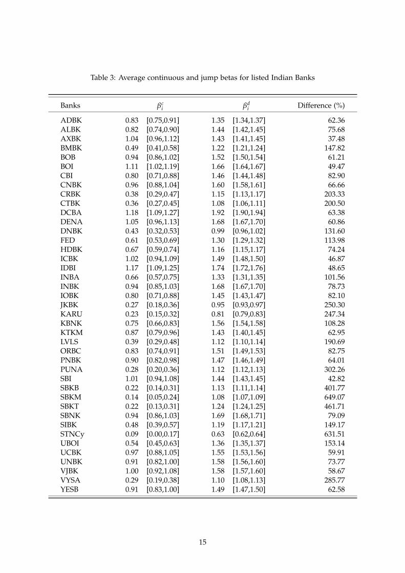
Table 3: Average continuous and jump betas for listed Indian Banks
Banks βci βd
i Difference (%)
ADBK 0.83 [0.75,0.91] 1.35 [1.34,1.37] 62.36ALBK 0.82 [0.74,0.90] 1.44 [1.42,1.45] 75.68AXBK 1.04 [0.96,1.12] 1.43 [1.41,1.45] 37.48BMBK 0.49 [0.41,0.58] 1.22 [1.21,1.24] 147.82BOB 0.94 [0.86,1.02] 1.52 [1.50,1.54] 61.21BOI 1.11 [1.02,1.19] 1.66 [1.64,1.67] 49.47CBI 0.80 [0.71,0.88] 1.46 [1.44,1.48] 82.90CNBK 0.96 [0.88,1.04] 1.60 [1.58,1.61] 66.66CRBK 0.38 [0.29,0.47] 1.15 [1.13,1.17] 203.33CTBK 0.36 [0.27,0.45] 1.08 [1.06,1.11] 200.50DCBA 1.18 [1.09,1.27] 1.92 [1.90,1.94] 63.38DENA 1.05 [0.96,1.13] 1.68 [1.67,1.70] 60.86DNBK 0.43 [0.32,0.53] 0.99 [0.96,1.02] 131.60FED 0.61 [0.53,0.69] 1.30 [1.29,1.32] 113.98HDBK 0.67 [0.59,0.74] 1.16 [1.15,1.17] 74.24ICBK 1.02 [0.94,1.09] 1.49 [1.48,1.50] 46.87IDBI 1.17 [1.09,1.25] 1.74 [1.72,1.76] 48.65INBA 0.66 [0.57,0.75] 1.33 [1.31,1.35] 101.56INBK 0.94 [0.85,1.03] 1.68 [1.67,1.70] 78.73IOBK 0.80 [0.71,0.88] 1.45 [1.43,1.47] 82.10JKBK 0.27 [0.18,0.36] 0.95 [0.93,0.97] 250.30KARU 0.23 [0.15,0.32] 0.81 [0.79,0.83] 247.34KBNK 0.75 [0.66,0.83] 1.56 [1.54,1.58] 108.28KTKM 0.87 [0.79,0.96] 1.43 [1.40,1.45] 62.95LVLS 0.39 [0.29,0.48] 1.12 [1.10,1.14] 190.69ORBC 0.83 [0.74,0.91] 1.51 [1.49,1.53] 82.75PNBK 0.90 [0.82,0.98] 1.47 [1.46,1.49] 64.01PUNA 0.28 [0.20,0.36] 1.12 [1.12,1.13] 302.26SBI 1.01 [0.94,1.08] 1.44 [1.43,1.45] 42.82SBKB 0.22 [0.14,0.31] 1.13 [1.11,1.14] 401.77SBKM 0.14 [0.05,0.24] 1.08 [1.07,1.09] 649.07SBKT 0.22 [0.13,0.31] 1.24 [1.24,1.25] 461.71SBNK 0.94 [0.86,1.03] 1.69 [1.68,1.71] 79.09SIBK 0.48 [0.39,0.57] 1.19 [1.17,1.21] 149.17STNCy 0.09 [0.00,0.17] 0.63 [0.62,0.64] 631.51UBOI 0.54 [0.45,0.63] 1.36 [1.35,1.37] 153.14UCBK 0.97 [0.88,1.05] 1.55 [1.53,1.56] 59.91UNBK 0.91 [0.82,1.00] 1.58 [1.56,1.60] 73.77VJBK 1.00 [0.92,1.08] 1.58 [1.57,1.60] 58.67VYSA 0.29 [0.19,0.38] 1.10 [1.08,1.13] 285.77YESB 0.91 [0.83,1.00] 1.49 [1.47,1.50] 62.58
15

very low continuous beta, followed by KARU (0.81).
The jump betas of all banks are on average 151% percent higher than their continuous
betas, and the columns of average confidence intervals of continuous and jump betas in Table
3 show that there is no overlap between the confidence intervals of βci ann βi
dfor any bank.
This supports the hypothesis that the continuous and jump betas in the augmented CAPM
specification of equation (2) differ, and that a single factor CAPM model may miss information
which is important for effective portfolio diversification and pricing. As an exemplar consider
the confidence intervals for the average continuous and jump beta for all banks depicted in
Figure 2, and for the State Bank of India, the largest Indian bank, in Figure 3. The figures
show a volatile pattern of average betas for all banks and a stable level of continuous beta
from January 2004 to December 2012 for SBI, while the jump beta has both higher values and
relatively higher variability than the continuous beta in both figures.
5.2. Risk premia
The estimates of beta are now considered with respect to their explanatory power for observed
stock returns (see, for example, Black et al., 1972; Fama and MacBeth, 1973). The usual ap-
proach regresses the standard CAPM beta on stock returns, using a pooled OLS approach, as
follows
dpi,t = δ + φh βhi,t + vi,t, (14)
which we extend to incorporate the separation of market returns into continuous and jump
components below:
dpi,t = δ + φc βci,t + φd βd
i,t + ωi,t, (15)
where dpi indicates stock returns, βhi in equation (14) is the estimated single factor CAPM
beta, and βci , and βd
i in equation (15) denote the estimated continuous and jump betas, re-
spectively. The models should produce a constant value, δ, equal to the risk free rate, and
16

Figure 2: Confidence interval of average monthly βci and βd
i of all banks
Jan-04 Jan-05 Jan-06 Jan-07 Jan-08 Jan-09 Jan-10 Jan-11 Jan-12
estim
ated
CI o
f β
c and
βd
0
0.5
1
1.5
2
2.5
3
Figure 3: Confidence interval of monthly βci and βd
i of SBI from 2004 to 2012
Jan−04 Jan−05 Jan−06 Jan−07 Jan−08 Jan−09 Jan−10 Jan−11 Jan−120
0.5
1
1.5
2
2.5
3
estim
ated
CI o
f βc a
nd β
d
the coefficients on the beta estimates, φ’s, should indicate the relevant market risk premium
which are expected to be significantly positive.
We first estimate monthly standard single factor CAPM beta in order to compare the
results with the disentangled betas. The average values of the estimated standard CAPM
betas βhi,t for Indian banks are shown in Table 4. For all banks, the standard CAPM beta has
a value higher than the continuous beta and lower than the jump beta. Thus, it is clear that
ignoring the source (continuous or jump) of change in the market return may lead to an over-
estimate of systematic risk during continuous market movements, and under-estimate during
discontinuous market movements. The average standard beta across all Indian banks is 0.87,
while the average continuous beta is 0.69 and average jump beta is 1.36.
17

Table 4: Average monthly continuous, jump and standard CAPM betas for Indian banks
Bank βci βd
i βhi Bank βc
i βdi βh
i
ADBK 0.83 1.35 1.03 KARU 0.23 0.81 0.33ALBK 0.82 1.44 1.01 KBNK 0.75 1.56 0.96AXBK 1.04 1.43 1.18 KTKM 0.87 1.43 1.03BMBK 0.49 1.22 0.67 LVLS 0.39 1.12 0.55BOB 0.94 1.52 1.13 ORBC 0.83 1.51 1.04BOI 1.11 1.66 1.30 PNBK 0.90 1.47 1.07CBI 0.80 1.46 0.98 PUNA 0.28 1.12 0.47CNBK 0.96 1.60 1.16 SBI 1.01 1.44 1.14CRBK 0.38 1.15 0.54 SBKB 0.22 1.13 0.42CTBK 0.36 1.08 0.51 SBKM 0.14 1.08 0.31DCBA 1.18 1.92 1.40 SBKT 0.22 1.24 0.39DENA 1.05 1.68 1.25 SBNK 0.94 1.69 1.19DNBK 0.43 0.99 0.60 SIBK 0.48 1.19 0.63FED 0.61 1.30 0.79 STNCy 0.09 0.63 0.16HDBK 0.67 1.16 0.78 UBOI 0.54 1.36 0.74ICBK 1.02 1.49 1.16 UCBK 0.97 1.55 1.19IDBI 1.17 1.74 1.36 UNBK 0.91 1.58 1.13INBA 0.66 1.33 0.84 VJBK 1.00 1.58 1.21INBK 0.94 1.68 1.15 VYSA 0.29 1.10 0.43IOBK 0.80 1.45 1.01 YESB 0.91 1.49 1.09JKBK 0.27 0.95 0.39
The results imply that the predictive power of CAPM beta is derived mainly from its jump
component rather than the continuous component. The regression results for equations (14)
and (15) are reported in Table 5. We find positive and significant coefficients of continuous,
jump and CAPM betas in univariate regressions shown in models (1), (2) and (3). However,
when we regress the stock returns on continuous and jump betas together as shown in model
(4), although jump beta remains significant, the continuous beta no longer has a significant
coefficient. 4
5.3. The role of firm characteristics
There is substantial heterogeneity in the estimated continuous and discontinuous betas across
the banks although they belong to the same industry. Patton and Verardo (2012) suggest that
the variations in beta are associated with firm-specific news and stock fundamentals. We
18
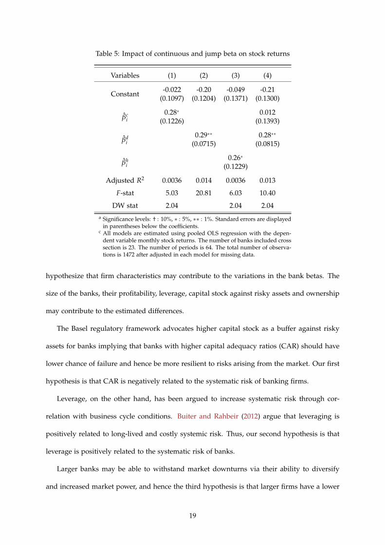
Table 5: Impact of continuous and jump beta on stock returns
Variables (1) (2) (3) (4)
Constant-0.022 -0.20 -0.049 -0.21
(0.1097) (0.1204) (0.1371) (0.1300)
βci
0.28∗ 0.012(0.1226) (0.1393)
βdi
0.29∗∗ 0.28∗∗
(0.0715) (0.0815)
βhi
0.26∗
(0.1229)
Adjusted R2 0.0036 0.014 0.0036 0.013
F-stat 5.03 20.81 6.03 10.40
DW stat 2.04 2.04 2.04
a Significance levels: † : 10%, ∗ : 5%, ∗∗ : 1%. Standard errors are displayedin parentheses below the coefficients.
c All models are estimated using pooled OLS regression with the depen-dent variable monthly stock returns. The number of banks included crosssection is 23. The number of periods is 64. The total number of observa-tions is 1472 after adjusted in each model for missing data.
hypothesize that firm characteristics may contribute to the variations in the bank betas. The
size of the banks, their profitability, leverage, capital stock against risky assets and ownership
may contribute to the estimated differences.
The Basel regulatory framework advocates higher capital stock as a buffer against risky
assets for banks implying that banks with higher capital adequacy ratios (CAR) should have
lower chance of failure and hence be more resilient to risks arising from the market. Our first
hypothesis is that CAR is negatively related to the systematic risk of banking firms.
Leverage, on the other hand, has been argued to increase systematic risk through cor-
relation with business cycle conditions. Buiter and Rahbeir (2012) argue that leveraging is
positively related to long-lived and costly systemic risk. Thus, our second hypothesis is that
leverage is positively related to the systematic risk of banks.
Larger banks may be able to withstand market downturns via their ability to diversify
and increased market power, and hence the third hypothesis is that larger firms have a lower
19

beta. Profitable firms may exhibit stable price behaviour, stemming from the confidence that
investors bestow on these stocks, making profitable firms less volatile than the market as
a whole, leading to hypothesis four that higher profitability is negatively related to beta.
Finally, we test whether similarly private versus government ownership reduces or increases
the systematic risk of a bank, as investors may have different degrees of confidence on these
two ownership modes.
Incorporating these firm characteristic factors, we estimate the following regression model:
βi,t = α +m
∑i=1
γXi,t + ui,t, (16)
for both jump beta and continuous beta separately, where Xi,t are the firm characteristic vari-
ables of ith bank at time t. We collect data on the firm characteristics for 23 Indian banks from
Datastream, and regress the jump beta or continuous beta on firm size, profitability, lever-
age, ownership and CAR separately. Firm size is represented by market capitalization in log
form. Leverage is computed as the ratio of total debt to market capitalization. Profitability is
measured in percentage of the return on assets (RoA), computed as earnings before interest
tax and depreciation and amortization (EBITDA) divided by market value of assets. We use a
dummy variable for nationalized versus private ownership of the banks and CAR is directly
extracted from Datastream. The summary statistics for the firm characteristics are reported in
Table 6.
Table 6: Summary statistics of firm characteristics
CAR Lev RoA Size RV
Mean 8.68 1.30 1.90 4.29 0.0105Median 8.54 0.96 1.85 4.18 0.0077Maximum 19.11 24.43 6.32 7.48 0.1877Minimum 0 0.01 0.71 0.70 0Std. Dev. 3.30 1.48 0.67 1.28 0.0120
a CAR denotes the capital adequacy ratio, RoA denotes the return on asset, Lev denotes the leverage ratio, Sizedenotes the logarithm of market capitalization, and RV denotes the realized variation.
20

In addition to firm characteristics, we consider the potential role of individual stock volatil-
ity. A firm that is highly volatile may show a greater reaction when the market moves. Alter-
natively, volatile stocks may be largely influenced by idiosyncratic factors rather than market
conditions, and thus exhibit lower beta values. Thus our final form of equation (16) takes the
following form:
βi,t = α + γ1CARi,t + γ2Levi,t + γ3RoAi,t + γ4Sizei,t + γ5Privatei,t + γ6RVi,t + ui,t, (17)
incorporating capital assets ration (CAR), leverage (Lev), return on assets (RoA), size (Size)
and RVi,t is realized variation for the ith bank at time t.
Table 7 reports the regression results on the relationship between betas and firm charac-
teristics. The first column reports the results for continuous beta and the second column the
results for jump beta. In the continuous beta specification we additionally include an AR(1)
term to tackle the autocorrelation in the error term. The table reports White adjusted standard
errors.
The results in Table 7 show that relationship between continuous beta and leverage is
positive and significant, at the 10% significance level, while the relationship of continuous
beta with CAR is negative and and significant at the 5% level. A decrease of one unit in the
leverage ratio is estimated to lead to a decrease of 0.04 in the continuous beta, assessed at the
mean value of leverage, this is equivalent to a decrease in the leverage ratio for Indian banks
from 1.2 to 1 resulting in a decrease in continuous beta of 0.008. It is immediately apparent
that a large change in leverage would be required to alter beta to an economically meaningful
extent. Similarly, although the relationship between continuous beta and CAR is statistically
significant, and negative, the change required in CAR to obtain an economically meaningful
reduction in beta is relatively large; an increase in CAR from its mean value of 8.6 to 9.6 results
in a small 0.02 decrease in continuous beta.
21
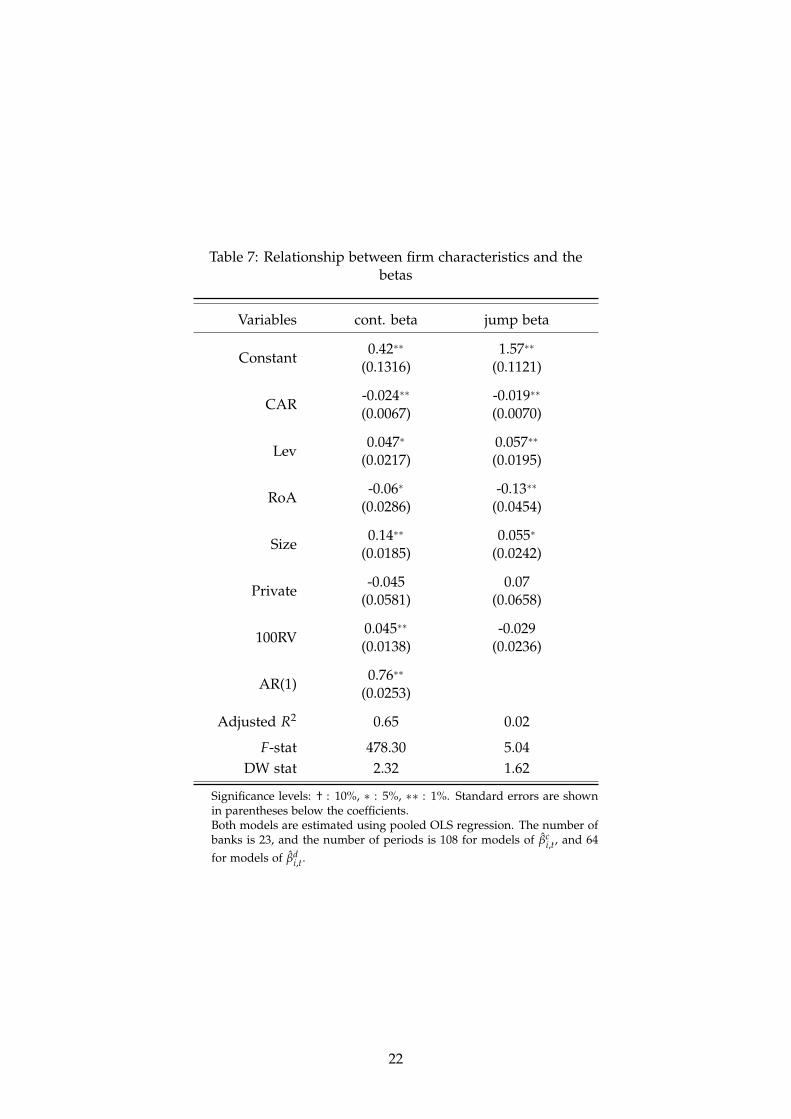
Table 7: Relationship between firm characteristics and thebetas
Variables cont. beta jump beta
Constant0.42∗∗ 1.57∗∗
(0.1316) (0.1121)
CAR-0.024∗∗ -0.019∗∗
(0.0067) (0.0070)
Lev0.047∗ 0.057∗∗
(0.0217) (0.0195)
RoA-0.06∗ -0.13∗∗
(0.0286) (0.0454)
Size0.14∗∗ 0.055∗
(0.0185) (0.0242)
Private-0.045 0.07
(0.0581) (0.0658)
100RV0.045∗∗ -0.029(0.0138) (0.0236)
AR(1)0.76∗∗
(0.0253)
Adjusted R2 0.65 0.02
F-stat 478.30 5.04DW stat 2.32 1.62
Significance levels: † : 10%, ∗ : 5%, ∗∗ : 1%. Standard errors are shownin parentheses below the coefficients.Both models are estimated using pooled OLS regression. The number ofbanks is 23, and the number of periods is 108 for models of βc
i,t, and 64for models of βd
i,t.
22

Profitability (RoA), size and volatility all have significant effects on continuous beta. The
negative coefficient of RoA and positive coefficient of market capitalization indicate that banks
of larger size but less profitability show higher sensitivities towards continuous market move-
ments. The volatility measure, RV, is a significant and positive factor for the continuous beta,
indicating that higher price volatility results in higher continuous risk for these banks. Private
versus government ownership has no significant relationship with beta.
Each of the explanatory variables, leverage, CAR, RoA and size also have significant effects
on jump beta – volatility, however, does not. The signs are the same as those for the continuous
beta estimates; increased CAR and RoA reduce jump beta, while decreased leverage and size
increase jump beta. The effects of CAR are slightly smaller than in the continuous case,
thus increasing bank capital has even lower impact here on reducing the reaction to market
discontinuities than in the continuous case. The leverage effect is only slightly higher than
in the continuous case. Interestingly the jump beta of more profitable firms is twice that of
the continuous betas – profitability reduces the reaction to market discontinuities – providing
evidence for the case that profitability provides a better buffer against these events. At the
same time, the coefficient on size almost halves for jump betas compared with continuous
betas. While in both continuous and jump beta cases larger, less profitable firms have lower
betas than their comparator firms, in the continuous beta case this effect is mainly due to size
effects (supporting the hypothesis that larger firms are less able to diversify away from the
market) and in the jump beta case the effect is mainly due to RoA (supporting the hypothesis
that profits provide a buffer from unexpected market movements).
Our investigation quantifies the importance of the well-recognised decomposition of finan-
cial price movements into continuous and jump components. We test whether separating the
beta estimates for these two components is warranted and unambiguously reject the hypoth-
esis that the jump beta and continuous beta are the same using data for the Indian banking
sector. The evidence strongly suggests that jump beta is higher than continuous beta, and that
23

it has more explanatory power over returns, consistent with the view that discontinuities in fi-
nancial prices are indicative of new information entering the market as in Patton and Verardo
(2012) and the evidence for US markets in Todorov and Bollerslev (2010) and Alexeev et al.
(2014).
We estimate the continuous and jump betas for an emerging market, and moreover, the
banking sector of that market which bears a high responsibility for effectively funding future
growth in India. Investigating the banking market specifically ties our results firmly to propo-
sitions for reducing systematic risk in that sector, with a view to reducing systemic risk in
the economy as a whole. We find that recent proposals to reduce systemic risk via increasing
capital requirements or reducing leverage in the banking sector would have the desired effect
of reducing the systematic risk in the sector for both continuous and jump betas, but either
the changes in capital or leverage required to produce economically meaningful results are
very large or there is a substantial non-linearity in the relationship between these variables
and systematic risk which is not captured by either this or other existing frameworks.
6. Conclusion
New tools allow the separate estimation of the beta on the continuous and jump component
of the underlying price process which characterises financial market data. The small existing
literature for the US in Todorov and Bollerslev (2010) and Alexeev et al. (2014) estimate higher
jump beta than continuous beta. This paper confirms a similar finding for Indian banking
stocks. The focus on the Indian banking sector links the results to an important emerging
economy with a high reliance on the banking sector for funding future growth, and con-
temporary issues concerning regulatory proposals for reducing systemic risk in international
banking sectors.
Using 5-minute stock price data for 41 listed Indian banks for 2004-2012 we establish evi-
dence of jumps in the Indian equity markets, consistent with existing evidence for developed
24

markets and as yet a small range of equities in emerging market. The results show that the
proportion of days containing a jump, at 4.85% of trading days, is not dissimilar to the evi-
dence for developed economies – and that the proportion of jumps did not increase during
the GFC, also consistent with the small existing literature concerning jump behaviour during
crisis periods.
The estimates of separate continuous and jump betas for the Indian banks show that on av-
erage jump beta exceeds continuous beta by 151%, and the confidence band on these estimate
rarely overlap for any of the individual stocks. We conclude that the reaction of individual
stocks to discontinuities in the market indicator price is substantially higher than the reaction
to continuous movements. This is consistent with the documented strong association of jumps
with news events, particularly unanticipated news, and the learning model posited in Patton
and Verardo (2012) which anticipates temporarily increased beta for stocks around the time of
earnings announcements. Our study differs from theirs in that we condition the differing beta
estimates on the existence of jumps, rather than on the existence of a news announcement
(there is clearly overlap between these groups but it is by no means complete).
The estimated continuous and jump betas are related positively to firm size and leverage,
and negatively to capital adequacy and profitability. Smaller profitable firms, with lower
leverage and strong capital will have lower betas. However, the effect of size on beta is twice
as large for continuous beta than jump beta, and the effect of profitability is twice as strong
for jump beta than continuous beta. These findings have bearing on the debate concerning
future regulatory practice for the banking sector in reducing systemic risk. Our results show
that proposals to increase bank capital and decrease leverage will act to reduce the systematic
risk in the Indian banking sector, with capital slightly more effective against continuous risk
and leverage slightly more effective against jump risk, but the extent of the reduction in betas
that can be produced in this manner are economically quite small. If the linear specification
proposed in this paper is correct the required reduction in leverage or increase in capital to
25

produce a economically meaningful impact on jump or continuous beta is beyond the scope
of current policy discussions. The behaviour of beta in response to leverage and capital would
need to be highly non-linear to prompt the required regulatory response – the existence of
such non-linearities is a scope for further research.
Notes
1The exchange rate was US$1=59.5260 Indian rupee as of 30/06/2013.
2Although we have calculated both daily and monthly time varying betas, in common with Todorov and
Bollerslev (2010) and Alexeev et al. (2014) we find that the volatility in the daily beta estimates favours the use of
the monthly betas for analysis.
3Unfortunately access to the firm characteristic data for STNCy is limited, restricting subsequent analysis. Of
the 108 months in our sample period, we have data for STNCy in 31 months, and hence estimate βc for that
subsample.
4Extending the set of potential explanatory variables to include firm characteristics covered in the next section
does not affect these conclusions. Results available from the authors on request.
References
Aït-Sahalia, Y. and Jacod, J. (2012), ‘Analyzing the Spectrum of Asset Returns: Jump and
Volatility Components in High Frequency Data’, Journal of Economic Literature 50(4), 1007–
50.
Alexeev, V., Dungey, M. and Yao, W. (2014), Continuous and Jump Betas with Applications
for Portfolio Management, working paper, University of Tasmania.
Andersen, T. G. and Bollerslev, T. (1998), ‘Deutsche Mark-Dollar Volatility: Intraday Activity
Patterns, Macroeconomic Announcements, and Longer Run Dependencies’, The Journal of
Finance 53(1), 219–265.
Andersen, T. G., Bollerslev, T. and Diebold, F. X. (2007), ‘Roughing It Up: Including Jump
26

Components in the Measurement, Modeling, and Forecasting of Return Volatility’, The Re-
view of Economics and Statistics 89(4), 701–720.
Andersen, T. G., Bollerslev, T., Diebold, F. X. and Labys, P. (2001), ‘The Distribution of Realized
Exchange Rate Volatility’, Journal of the American Statistical Association 96(453), 42–55.
Andersen, T. G., Bollerslev, T., Diebold, F. X. and Wu, J. G. (2005), A Framework for Exploring
the Macroeconomic Determinants of Systematic Risk, Technical report, National Bureau of
Economic Research.
Barada, Y. and Yasuda, K. (2012), ‘Testing for Levy Type Jumps in Japanese Stock Market
under the Financial Crisis Using High Frequency Data’, International Journal of Innovative
Computing Information and Control 8(3 B), 2215–2223.
Barndorff-Nielsen, O. E. and Shephard, N. (2004a), ‘Econometric Analysis of Realized Co-
variation: High Frequency Based Covariance, Regression, and Correlation in Financial Eco-
nomics’, Econometrica 72(3), 885–925.
Barndorff-Nielsen, O. E. and Shephard, N. (2004b), ‘Power and Bipower Variation with
Stochastic Volatility and Jumps’, Journal of Financial Econometrics 2(1), 1–37.
Barndorff-Nielsen, O. E. and Shephard, N. (2006), ‘Econometrics of Testing for Jumps in Fi-
nancial Economics Using Bipower Variation’, Journal of Financial Econometrics 4(1), 1–30.
Bianconi, M., Yoshino, J. A. and de Sousa, M. O. M. (2011), BRIC and the U.S. Financial Crisis:
An Empirical Investigation of Stocks and Bonds Markets, Discussion Papers Series, Depart-
ment of Economics, Tufts University 0764, Department of Economics, Tufts University.
BIS (2013), ITriennial Central Bank Survey: Foreign Exchange Turnover in April 2013: Prelim-
inary Global Results, Report, Bank for International Settlements.
Black, A., Chen, J., Gustap, O. and Williams, J. M. (2012), The Importance of Jumps in Mod-
elling Volatility during the 2008 Financial Crisis, Technical report.
27

Black, F., Jensen, M. C. and Scholes, M. S. (1972), Studies in the Theory of Capital Markets, Praeger
Publishers Inc., chapter The Capital Asset Pricing Model: Some Empirical Tests.
Bollerslev, T., Engle, R. F. and Wooldridge, J. M. (1988), ‘A Capital Asset Pricing Model with
Time-varying Covariances’, Journal of Political Economy pp. 116–131.
Bollerslev, T. and Zhang, B. Y. (2003), ‘Measuring and Modeling Systematic Risk in Factor
Pricing Models Using High-frequency Data’, Journal of Empirical Finance 10(5), 533–558.
Buchanan, B. G., English II, P. C. and Gordon, R. (2011), ‘Emerging Market Benefits, Investa-
bility and the Rule of Law’, Emerging Markets Review 12(1), 47–60.
Buiter, W. and Rahbeir, E. (2012), Debt, Financial Crisis and Economic Growth, in ‘Conference
on Monetary Policy and the Challenge of Economic Growth at the South Africa Reserve
Bank, Pretoria, South Africa, November’, pp. 1–2.
Chowdhury, B. (2014), Continuous and Discontinuous Beta Estimation Using High Frequency
Data: Evidence from Japan. manuscript.
Dungey, M., McKenzie, M. and Smith, V. (2009), ‘Empirical Evidence on Jumps in the Term
Structure of the US Treasury Market’, Journal of Empirical Finance 16, 430–445.
Fabozzi, F. J. and Francis, J. C. (1978), ‘Beta as a Random Coefficient’, Journal of Financial and
Quantitative Analysis 13(01), 101–116.
Faff, R., Ho, Y. K. and Zhang, L. (1998), ‘A Generalised Method Of Movements (GMM) Test Of
The Three-Moment Capital Asset Pricing Model (CAPM) In The Australian Equity Market’,
Asia Pacific Journal of Finance 1, 45–60.
Fama, E. F. and French, K. R. (1993), ‘Common Risk Factors in the Returns on Stocks and
Bonds’, Journal of Financial Economics 33(1), 3–56.
28

Fama, E. F. and MacBeth, J. D. (1973), ‘Risk, Return, and Equilibrium: Empirical Tests’, Journal
of Political Economy 81(3), pp. 607–636.
Fraser, P., Hamelink, F., Hoesli, M. and MacGregor, B. (2000), Time-varying Betas and Cross-
sectional Return-risk Relation: Evidence from the UK, Université de Genève, Faculté des sciences
économiques et sociales, Section des hautes études commerciales.
Friend, I. and Westerfield, R. (1980), ‘Co-skewness and Capital Asset Pricing’, The Journal of
Finance 35(4), 897–913.
Hanousek, J. and Novotný, J. (2012), ‘Price Jumps in Visegrad-country Stock Markets: An
Empirical Analysis’, Emerging Markets Review 13(2), 184–201.
Harvey, C. R. and Siddique, A. (2000), ‘Conditional Skewness in Asset Pricing Tests’, The
Journal of Finance 55(3), 1263–1295.
Huang, X. and Tauchen, G. (2005), ‘The Relative Contribution of Jumps to Total Price Variance’,
Journal of Financial Econometrics 3(4), 456–499.
Kraus, A. and Litzenberger, R. H. (1976), ‘Skewness Preference and the Valuation of Risk
Assets’, The Journal of Finance 31(4), 1085–1100.
Liao, Y., Anderson, H. M. and Vahid, F. (2010), Do Jumps Matter? Forecasting Multivariate Re-
alized Volatility allowing for Common Jumps, Technical Report 11/10, Monash University,
Department of Econometrics and Business Statistics.
Lintner, J. (1965), ‘The Valuation of Risk Assets and the Selection of Risky Investments in Stock
Portfolios and Capital Budgets’, Review of Economics and Statistics 47(1), pp. 13–37.
Mensi, W., Hammoudeh, S., Reboredo, J. C. and Nguyen, D. K. (2014), ‘Do Global Factors
Impact BRICS Stock Markets? A Quantile Regression Approach’, Emerging Markets Review
19(C), 1–17.
29

Merton, R. C. (1976), ‘Option Pricing When Underlying Stock Returns Are Discontinuous’,
Journal of Financial Economics 3, 125 – 144.
Novotný, J., Hanousek, J. and Kocenda, E. (2013), Price Jump Indicators: Stock Market Empir-
ics During the Crisis, William Davidson Institute Working Papers Series wp1050, William
Davidson Institute at the University of Michigan.
Patton, A. J. and Verardo, M. (2012), ‘Does Beta Move with News? Firm-specific Information
Flows and Learning About Profitability’, Review of Financial Studies 25, 2789–2839.
Rathinam, F. X. and Raja, A. V. (2010), ‘Law, Regulation and Institutions for Financial Devel-
opment: Evidence from India’, Emerging Markets Review 11(2), 106–118.
Ross, S. A. (1976), ‘The Arbitrage Theory of Capital Asset Pricing’, Journal of Economic Theory
13(3), 341–360.
Sharpe, W. F. (1964), ‘Capital Asset Prices: A Theory of Market Equilibrium under Conditions
of Risk’, The Journal of Finance 19(3), 425–442.
Todorov, V. and Bollerslev, T. (2010), ‘Jumps and Betas: A New Framework for Disentangling
and Estimating Systematic Risks’, Journal of Econometrics 157(2), 220–235.
Zhou, H. and Zhu, J. Q. (2012), ‘An Empirical Examination of Jump Risk in Asset Pricing
and Volatility Forecasting in China’s Equity and Bond Markets’, Pacific-Basin Finance Journal
20(5), 857–880.
30

TASMANIAN SCHOOL OF BUSINESS AND ECONOMICS WORKING PAPER SERIES
2014-09 VAR Modelling in the Presence of China’s Rise: An Application to the Taiwanese Economy. Mardi Dun-gey, Tugrul Vehbi and Charlton Martin
2014-08 How Many Stocks are Enough for Diversifying Canadian Institutional Portfolios? Vitali Alexeev and Fran-cis Tapon
2014-07 Forecasting with EC-VARMA Models, George Athanasopoulos, Don Poskitt, Farshid Vahid, Wenying Yao
2014-06 Canadian Monetary Policy Analysis using a Structural VARMA Model, Mala Raghavan, George Athana-sopoulos, Param Silvapulle
2014-05 The sectorial impact of commodity price shocks in Australia, S. Knop and Joaquin Vespignani
2014-04 Should ASEAN-5 monetary policymakers act pre-emptively against stock market bubbles? Mala Raghavan and Mardi Dungey
2014-03 Mortgage Choice Determinants: The Role of Risk and Bank Regulation, Mardi Dungey, Firmin Doko Tchatoka, Graeme Wells, Maria B. Yanotti
2014-02 Concurrent momentum and contrarian strategies in the Australian stock market, Minh Phuong Doan, Vi-tali Alexeev, Robert Brooks
2014-01 A Review of the Australian Mortgage Market, Maria B. Yanotti
2014-10 Contagion and Banking Crisis - International Evidence for 2007-2009 , Mardi Dungey and Dinesh Gaju-rel
2014-11 The impact of post‐IPO changes in corporate governance mechanisms on firm performance: evidence from young Australian firms, Biplob Chowdhury, Mardi Dungey and Thu Phuong Pham
2014-12 Identifying Periods of Financial Stress in Asian Currencies: The Role of High Frequency Financial Market Data, Mardi Dungey, Marius Matei and Sirimon Treepongkaruna
2014-13 OPEC and non‐OPEC oil production and the global economy, Ronald Ratti and Joaquin Vespignani
2014-14 VAR(MA), What is it Good For? More Bad News for Reduced‐form Estimation and Inference, Wenying Yao, Timothy Kam and Farshid Vahid