High energy QCD: multiplicity distribution and entanglement entropy

E. Gotsman1, ∗ and E. Levin1, 2, †

1Department of Particle Physics, School of Physics and Astronomy,Raymond and Beverly Sackler Faculty of Exact Science, Tel Aviv University, Tel Aviv, 69978, Israel

2 Departamento de Física, Universidad Tecnica Federico Santa María andCentro Científico-Tecnologico de Valparaíso, Casilla 110-V, Valparaiso, Chile

(Dated: June 23, 2020)

In this paper we show that QCD at high energies leads to the multiplicity distribution σnσin

=1N

(N − 1N

)n−1, (where N denotes the average number of particles), and to entanglement entropyS = lnN , confirming that the partonic state at high energy is maximally entangled. However, thevalue of N depends on the kinematics of the parton cascade. In particular, for DIS N = xG(x,Q) ,where xG is the gluon structure function, while for hadron-hadron collisions, N ∝ Q2

S(Y ), where Qsdenotes the saturation scale. We checked that this multiplicity distribution describes the LHC datafor low multiplicities n < (3÷ 5)N , exceeding it for larger values of n. We view this as a result ofour assumption, that the system of partons in hadron-hadron collisions at c.m. rapidity Y = 0 isdilute. We show that the data can be described at large multiplicities in the parton model, if we donot make this assumption.

PACS numbers: 13.60.Hb, 12.38.Cy

Contents

I. Introduction 1

II. The QCD parton cascade 3A. QCD cascade for fast moving large dipole 3

1. General approach 32. Several first iterations 43. Solution 6

B. Multiplicity distribution and entropy of the parton cascade 6C. QCD motivated parton model 8D. Mutiplicity distribution for the parton cascade in DIS 8

III. Multiplicity distribution in Colour Glass Condensate (CGC) approach 11

IV. Multiplicity distribution in hadron-hadron scattering 12A. The interaction of two dipoles at high energies 12B. Hadron - hadron collisions 13C. Comparison with the experimental data 14D. Back to QCD motivated parton model 16

V. Conclussions 18

VI. Acknowledgements 19

References 19

I. INTRODUCTION

Over the past several years new ideas have been developed in the high energy and nuclear physics community, whichsuggest a robust relation between the principle features of high energy scattering and entanglement properties of thehadronic wave function [1–17]. The main idea, which we explore in this paper, is the intimate relation between theentropy in the parton approach[18–21] and the entropy of entanglement in a proton wave function[5].

arX

iv:2

006.

1179

3v1

[he

p-ph

] 2

1 Ju

n 20

20

2

This relation materialized as the resolution of the following difficulty in our understanding of high energy scattering:on one hand, the proton is a pure state and it is described by a completely coherent wave function with zero entropy,but, on the other hand, the DIS experiments are successfully described, treating the proton as a incoherent collectionof quasi-free partons. This ensemble has non vanishing entropy, and Ref.[5] proposes, that the origin of this entropyis the entanglement between the degrees of freedom one observes in DIS (partons in the small spatial region of theproton), and the rest of the proton wave function, which is not measured in the DIS experiments.

In other words, the hadron in the rest frame is described by a pure state |ψ〉 with density matrix ρ = |ψ〉〈ψ| andzero von Neumann entropy S = −tr [ρ ln ρ] = 0. In DIS at Bjorken x and momentum transfer q2 = −Q2 probes onlya part of the proton’s wave function; let us denote it A. In the proton’s rest frame the DIS probes the spatial regionA localized within a tube of radius ∼ 1/Q and length ∼ 1/(mx) [22, 23], where m is the proton’s mass. The inclusiveDIS measurement thus sums over the unobserved part of the wave function localized in the region B complementaryto A, so we have access only to the reduced density matrix ρA = trBρ, and not the entire density matrix ρ = |ψ〉〈ψ|.In Ref.[5] it is proposed that

SA = −trB [ρA ln ρA] = Sparton cascade (1)

Eq. (1), in spite of its general form, means that we can estimate the entropy and multiplicity distribution of theproduced gluons using the parton wave function in the initial state. In addition , we can obtain a thermal distributionof the produced particles in the high energy collision in spite of the fact, that the number of secondary interactions inproton-proton collisions is rather low, and cannot provide the thermalization due to the interaction in the final state.

It has been demonstrated in Refs.[6, 10, 11, 16] that these ideas are in qualitative and, partly, in quantitativeagreement with the available experimental data.

The goal of this paper is to study the multiplicity distribution and the entanglement entropy in the effective theoryfor QCD at high energies (see Ref.[24] for a general review). Such a theory exists in two different formulations: theCGC/saturation approach [25–30], and the BFKL Pomeron calculus [31–45].

We believe that the CGC/saturation approach provides a more general pattern [43, 44] for the treatment of highenergy QCD. However, in this paper we restrict ourself to the BFKL Pomeron calculus, which has a more directcorrespondence with the parton approach, and has been used in Ref.[5].

Fortunately, in Ref.[44] it was shown, that these two approaches are equivalent for the description of the scatteringamplitude

Y ≤ 2

∆BFKL

ln

(1

∆2BFKL

)(2)

where ∆BFKL denotes the intercept of the BFKL Pomeron.The main difference between the CGC approach and the parton QCD cascade for the topics dealt with in this

paper, is the fact that the CGC approach generates the non-diagonal elements of the density matrix (see for exampleRefs.[3, 9, 12, 17]), while for the parton cascade and, generally, in the BFKL Pomeron calculus the density matrix isdiagonal. Since in DIS experiments we can only measure the diagonal elements of density matrix, we can introducein the framework another kind of entropy:“ the entropy of ignorance"[17], which characterized this lack of knowledgeof the actual density matrix in DIS experiments. We will show below that the McLerran-Venugopalan approach[25],that is used in Ref.[17], leads to the same multiplicity distribution as the parton cascade.

The paper is organized as follows: In the next section we consider the entropy and multiplicity distributions in theQCD parton cascade. We show that in spite of the fact that in different kinematic regions, the QCD cascade leads toa different energy and dipole size dependence of the mean multiplicity, and the multiplicity distribution has a generalform:

σnσin

=1

N

(N − 1

N

)n−1

(3)

where N is the average number of partons. The entanglement entropy is equal to Sparton cascade = lnN , confirmingthat the partonic state at high energy is maximally entangled [5]. In the case of DIS we argue that N is equal tothe gluon structure function, but we can only prove the multiplicity distribution of Eq. (3), for the BFKL evolutionof this structure function. In section III we show that the CGC approach leads to the multiplicity distribution ofEq. (3). In section IV we consider hadron-hadron scattering. In the range of energy given by Eq. (2) we use theMueller-Patel-Salam-Iancu(MPSI) [36, 49] approach, using the formalism of Ref.[41]. We show that in the frameworkof this approach we have the distribution of Eq. (3) which can describe the experimental data for sufficiently low

3

multiplicities n ≤ (3 ÷ 5) < n > . However, we fail to describe the data for larger n. We conclude that the mainassumption of the MPSI approach, that a system of dilute partons are produced in the c.m. rapidity Y=0, is notvalid for large multiplicities at high energies of the LHC. Unfortunately, at the moment we have no theoretical toolto treat this scattering. However, in Ref.[50] an approach has been suggested, which allows us to describe the densesystem of partons in hadron-hadron collisions, as well as the dilute one. Developing this approach for the multiplicitydistribution, we are able to describe the data for large multiplicities. We summarize our results in the conclusions.

II. THE QCD PARTON CASCADE

A. QCD cascade for fast moving large dipole

1. General approach

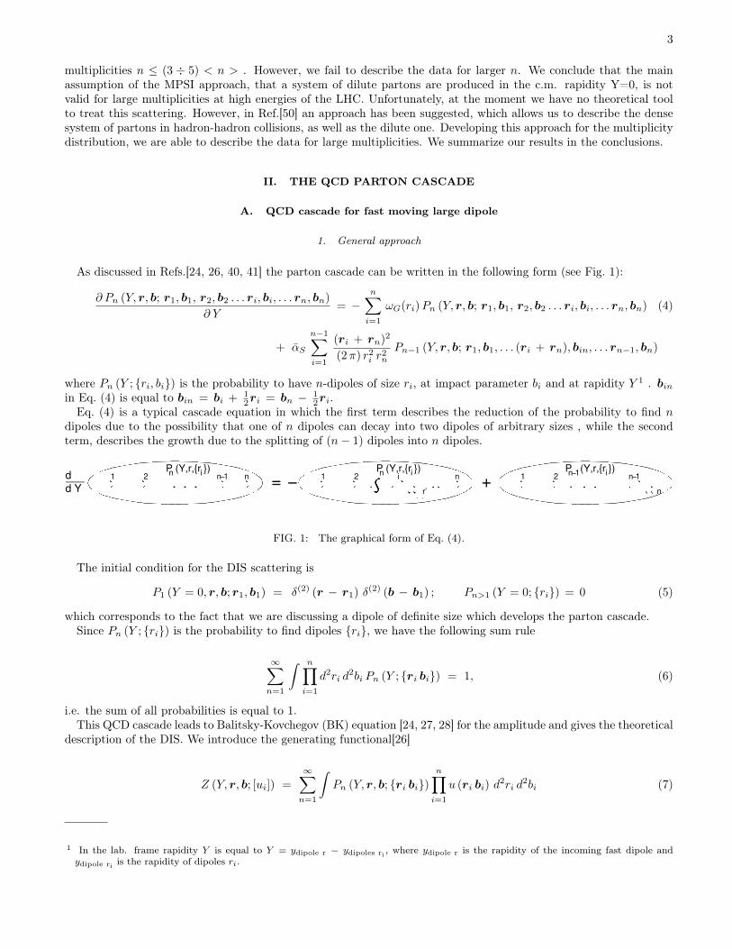
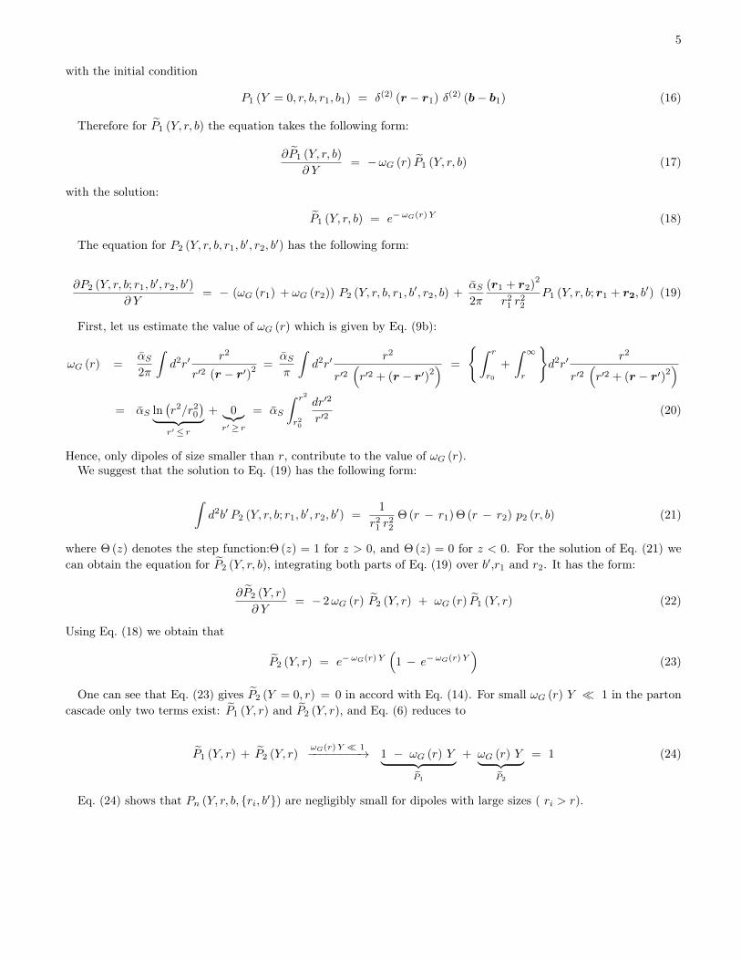
As discussed in Refs.[24, 26, 40, 41] the parton cascade can be written in the following form (see Fig. 1):

∂ Pn (Y, r, b; r1, b1, r2, b2 . . . ri, bi, . . . rn, bn)

∂ Y= −

n∑i=1

ωG(ri)Pn (Y, r, b; r1, b1, r2, b2 . . . ri, bi, . . . rn, bn) (4)

+ αS

n−1∑i=1

(ri + rn)2

(2π) r2i r

2n

Pn−1 (Y, r, b; r1, b1, . . . (ri + rn), bin, . . . rn−1, bn)

where Pn (Y ; {ri, bi}) is the probability to have n-dipoles of size ri, at impact parameter bi and at rapidity Y 1 . binin Eq. (4) is equal to bin = bi + 1

2ri = bn − 12ri.

Eq. (4) is a typical cascade equation in which the first term describes the reduction of the probability to find ndipoles due to the possibility that one of n dipoles can decay into two dipoles of arbitrary sizes , while the secondterm, describes the growth due to the splitting of (n− 1) dipoles into n dipoles.

d___d Y =1 2 n−1 n

P (Y,r,{r })n i

− 1 2 i nP (Y,r,{r })n i

r’+ 1 2 n−1

n

P (Y,r,{r })n−1 i

FIG. 1: The graphical form of Eq. (4).

The initial condition for the DIS scattering is

P1 (Y = 0, r, b; r1, b1) = δ(2) (r − r1) δ(2) (b − b1) ; Pn>1 (Y = 0; {ri}) = 0 (5)

which corresponds to the fact that we are discussing a dipole of definite size which develops the parton cascade.Since Pn (Y ; {ri}) is the probability to find dipoles {ri}, we have the following sum rule

∞∑n=1

∫ n∏i=1

d2ri d2bi Pn (Y ; {ri bi}) = 1, (6)

i.e. the sum of all probabilities is equal to 1.This QCD cascade leads to Balitsky-Kovchegov (BK) equation [24, 27, 28] for the amplitude and gives the theoretical

description of the DIS. We introduce the generating functional[26]

Z (Y, r, b; [ui]) =

∞∑n=1

∫Pn (Y, r, b; {ri bi})

n∏i=1

u (ri bi) d2ri d

2bi (7)

1 In the lab. frame rapidity Y is equal to Y = ydipole r − ydipoles ri , where ydipole r is the rapidity of the incoming fast dipole andydipole ri is the rapidity of dipoles ri.

4

where u (ri bi) ≡= ui is an arbitrary function. The initial conditions of Eq. (5) and the sum rules of Eq. (6) take tofollowing form for the functional Z:

Z (Y = 0, r, b; [ui]) = u (r, b) ; (8a)Z (Y, r, [ui = 1]) = 1; (8b)

Multiplying both parts of Eq. (4) by∏ni=1 u (ri bi) and integrating over ri and bi we obtain the following linear

functional equation[41];

∂Z (Y, r, b; [ui])

∂ Y=

∫d2r′K (r′, r − r′|r)

(− u (r, b) + u

(r′, b +

1

2(r − r′)

)u

(r − r′, b− 1

2r′))

δ Z

δ u (r, b);(9a)

K (r′, r − r′|r) =αS2π

r2

r′2 (r − r′)2; ωG (r) =

∫d2r′K (r′, r − r′|r) ; (9b)

Searching for the solution of the form Z ([u(ri, bi, Y )]) for the initial conditions of Eq. (8a), Eq. (9a) can be re-writtenas the non-linear equation [26]:

∂Z (Y, r, b; [ui])

∂ Y=

∫d2r′K (r′, r − r′|r)

{Z

(r′, b +

1

2(r − r′); [ui]

)Z

(r − r′, b− 1

2r′; [ui]

)− Z (Y, r, b; [ui])

}(10)

Therefore, the QCD parton cascade of Eq. (4) takes into account non-linear evolution. However, to obtain the BKequation for the scattering amplitude we need to introduce the scattering amplitude γ (ri, b), for the interaction ofthe dipole with the target at low energies. Using these amplitudes we can obtain the non-linear BK equation fromEq. (10), since [28]

N (Y, r, b) =

∞∑n=1

(−1)n−1

n!

∫ n∏i=1

(d2riγ (ri, b)

δ

δui

)Z (Y, r, b, [ui]) |ui=1 (11)

Using Eq. (9a) and Eq. (11) we derive the BK equation in the standard form:

∂

∂YN (r, b, Y ) =

∫d2r′K (r′, r − r′|r)

{N

(r′, b− 1

2(r − r′) , Y

)+N

(r − r′, b− 1

2r′, Y

)− N (r, b, Y )

−N(r − r′, b− 1

2r′, Y

)N

(r′, b− 1

2(r − r′) , Y

)}(12)

2. Several first iterations

Our goal is to find the solution to Eq. (4). In particular, for the multiplicity distribution and for the entropy wewish to find

Pn (Y, r) =

∫Pn(Y, r, b, {ri, b′

) n∏n=1

d2ri d2b′ (13)

Pn is the probability to find n dipoles of all possible sizes at the same values of the impact parameters and, beingsuch, it gives σn/σin, which is the multiplicity distribution in the QCD parton cascade. The initial and boundaryconditions for Pn (Y, r) follows from Eq. (5) and Eq. (6) and take the form:

P1 (Y = 0, r, b) = 1; Pn (Y = 0, r) = 0 for n > 1;

∞∑n=1

P1 (Y, r, b) = 1; (14)

First, let us find P1 (Y, r). The equation for P1 has the form:

∂P1 (Y, r, b, r1, b1)

∂ Y= −ωG (r1)P1 (Y, r, b, r1, b1) (15)

5

with the initial condition

P1 (Y = 0, r, b, r1, b1) = δ(2) (r − r1) δ(2) (b− b1) (16)

Therefore for P1 (Y, r, b) the equation takes the following form:

∂P1 (Y, r, b)

∂ Y= −ωG (r) P1 (Y, r, b) (17)

with the solution:

P1 (Y, r, b) = e−ωG(r)Y (18)

The equation for P2 (Y, r, b, r1, b′, r2, b

′) has the following form:

∂P2 (Y, r, b; r1, b′, r2, b

′)

∂ Y= − (ωG (r1) + ωG (r2)) P2 (Y, r, b, r1, b

′, r2, b) +αS2π

(r1 + r2)2

r21 r

22

P1 (Y, r, b; r1 + r2, b′) (19)

First, let us estimate the value of ωG (r) which is given by Eq. (9b):

ωG (r) =αS2π

∫d2r′

r2

r′2 (r − r′)2 =

αSπ

∫d2r′

r2

r′2(r′2 + (r − r′)

2) =

{∫ r

r0

+

∫ ∞r

}d2r′

r2

r′2(r′2 + (r − r′)

2)

= αS ln(r2/r2

0

)︸ ︷︷ ︸r′≤ r

+ 0︸︷︷︸r′≥ r

= αS

∫ r2

r20

dr′2

r′2(20)

Hence, only dipoles of size smaller than r, contribute to the value of ωG (r).We suggest that the solution to Eq. (19) has the following form:

∫d2b′ P2 (Y, r, b; r1, b

′, r2, b′) =

1

r21 r

22

Θ (r − r1) Θ (r − r2) p2 (r, b) (21)

where Θ (z) denotes the step function:Θ (z) = 1 for z > 0, and Θ (z) = 0 for z < 0. For the solution of Eq. (21) wecan obtain the equation for P2 (Y, r, b), integrating both parts of Eq. (19) over b′,r1 and r2. It has the form:

∂P2 (Y, r)

∂ Y= − 2ωG (r) P2 (Y, r) + ωG (r) P1 (Y, r) (22)

Using Eq. (18) we obtain that

P2 (Y, r) = e−ωG(r)Y(

1 − e−ωG(r)Y)

(23)

One can see that Eq. (23) gives P2 (Y = 0, r) = 0 in accord with Eq. (14). For small ωG (r) Y � 1 in the partoncascade only two terms exist: P1 (Y, r) and P2 (Y, r), and Eq. (6) reduces to

P1 (Y, r) + P2 (Y, r)ωG(r)Y � 1−−−−−−−−→ 1 − ωG (r) Y︸ ︷︷ ︸

P1

+ ωG (r) Y︸ ︷︷ ︸P2

= 1 (24)

Eq. (24) shows that Pn (Y, r, b, {ri, b′}) are negligibly small for dipoles with large sizes ( ri > r).

6

3. Solution

We suggest to look for the general solution in the form:

Pn(Y, r, b; {ri, b′}

)=

n∏i=1

Θ (r − ri)1

r2i

pn (Y, r, ) (25)

For such a solution we can obtain from Eq. (4) the following equations for Pn (Y, r):

∂Pn (Y, r)

∂ Y= −nωG (r) Pn (Y, r) + (n − 1)ωG (r) Pn−1 (Y, r) (26)

Introducing the Laplace transform:

Pn (Y, r) =

∫ ε+ i∞

ε− i∞

dω

2π ipn (ω, r) (27)

we re-write Eq. (26) in the form:

∂pn (ω, r)

∂ Y= −nωG (r) pn (, r) + (n − 1)ωG (r) pn−1 (ω, r) (28)

Eq. (28) has the solution:

pn (ω, r) = (n− 1)!

n∏m=1

1

ω + mωG (r)(29)

Taking the inverse Laplace transform of function e−ωG(r)Y(1 − e−ωG(r)Y

)n−1, we have∫ ∞

0

dY e−ω Y e−ωG(r)Y(

1 − e−ωG(r)Y)n−1

= (n− 1)!

n∏m=1

ωG (r)

ω + mωG (r)= pn (ω, r) (30)

Hence we have the following solution:

Pn (Y, r) = e−ωG(r)Y(

1 − e−ωG(r)Y)n−1

(31)

It is easy to see that Eq. (31) satisfies the initial conditions and the sum rules of Eq. (14).

B. Multiplicity distribution and entropy of the parton cascade

As has been mentionedσnσin

= Pn (Y, r) (32)

and, therefore, determines the multiplicity distribution. Calculating the average N

N =

∞∑n=1

nσnσin

=

∞∑n=1

n Pn (Y, r) = eω(r)Y (33)

we see that this distribution can be written in the form:

σnσin

=1

N

(N − 1

N

)n−1

=1

N

(N

N + 1

)n, (34)

7

where we have denoted N = N − 1.We can compare Eq. (34) with the general form of the negative binomial distribution (NBD)

PNBD (r, n, n) =

(r

r + 〈n〉

)rΓ (n+ r)

n! Γ (r)

(〈n〉

r + 〈n〉

)n, (35)

One can see that Eq. (34) can be re-written as

σnσin

=N

N + 1PNBD

(1, N , n

), (36)

where σn is the cross section for producing n hadrons in a collision, and σin is the inelastic cross section. Thereforeat large N our distribution is close to the negative binomial distribution with number of failures r = 1 and withprobability of success p = N/

(N + 1

). Eq. (34) coincides with the multiplicity distribution in the parton model (see

below and Ref.[5]). The difference is only in the expression for the average multiplicity (N).Having Eq. (34) we can calculate the von Neumann entropy of the parton cascade (see Eq. (1)), given by the Gibbs

formula

Sparton cascade, = −∑n

pn ln pn (37)

where pn is the probabilities of micro-states. In the parton cascade we can identify pn with Pn (Y, r) , reducingEq. (38) to the following expression:

Sparton cascade = −∑n

Pn (Y, r) ln Pn (Y, r) =∑n

(ln N − n ln

(N

N + 1

))1

N

(N

N + 1

)n= ln N + ln

(N

N + 1

)(1 +

1

N

)N� 1−−−−→ ln (N − 1) = ωG (r) Y (38)

exact

asymptotics

2 4 6 8 10

0

2

4

6

8

10

ln N = ωG(r) Y

S

FIG. 2: Entropy S versus lnN = ωG (r) Y (see Eq. (38). Sasymp = lnN = ωG (r) Y .

Eq. (38) shows that at large Y all probabilities Pn become equal and small, of the order of Pn ∼ 1N . It is well

known that this equipartitioning of micro-states maximizes the von Neumann entropy and describes the maximallyentangled state. We thus conclude that at large Y the fast dipole represents a maximally entangled quantum state ofpartons.

8

C. QCD motivated parton model

The main assumption of the parton model[19–21] is that all partons have average transverse momentum which doesnot depend on energy. Therefore, we can obtain the parton model from the QCD cascade assuming that the unknownconfinement of gluons leads to the QCD cascade for the dipole of fixed size. In this case the cascade equation takethe following form:

dPn (Y )

dY= −∆nPn (Y ) + (n− 1) ∆Pn−1 (Y.) (39)

where Pn (Y ) is the probability to find n dipoles (of a fixed size in our model) at rapidity Y and ∆ = ωG (r = r0).Using the Laplace transform of Eq. (27) we obtain the solution to Eq. (39) in the form:

Pn (ω) = (n− 1)!

n∏m=1

1

ω + m∆(40)

Using Eq. (30), we see that the solution of Eq. (39) has the form:

σnσin

≡ Pn (Y ) = e−∆Y(1 − e−∆Y

)n−1=

1

N

(N − 1

N

)n−1

(41)

which is a direct generalization of Eq. (31). In Eq. (41), N is the average number of the partons, which is equal toN = exp (∆Y ). In the parton model the average number of partons is related to the deep inelastic structure function.Therefore, in Ref.[5] it is assumed that

N = xG(x,Q2

)(42)

where xG is the gluon structure function. In this case ∆ can be identified with the intercept of the BFKL Pomeron[31].One can see that N = exp (ωG (r) Y ) this is certainly not the same as a solution of the QCD evolution for the gluonstructure function.

D. Mutiplicity distribution for the parton cascade in DIS

As we have seen (see Eq. (25)) our solution describes the evolution in the system of partons with smaller sizes ofdipoles than the initial fastest dipole. On the other side, only partons of larger than initial parton size, contribute to thestructure function. In double log approximation the emission of such dipoles leads to xG ∝ exp

(2√αSY ln (R2/r2)

),

where R is the size of the target. We need to consider how the produced dipoles interact with the target. We measurethe gluon structure function in the experiment in which r2 of the fastest dipole is about r2 sim1/Q2 � R2. Since allri ≤ r the n produced dipoles interact with the target at rapidity Y and since ri < R the amplitude of this interactionis proportional to r2

i /R2. This fact completely changes the structure of the cascade. Let us illustrate this, considering

P2 (Y, r; r1, r2). The amplitude of interaction is proportional to ρ2(Y, r, b; r1, r2, b′) ≡ (r2

1 + r22)P2 (Y, r, b; r1, r2, b

′).Let us look at Eq. (19) for ri > r. The term with gluon ωG (ri) does not contribute since as we have discussed onlyri > r contribute in this term. Therefore the equation reduces to the following one:

∂ (ρ2(Y, r, b; r1, r2, b′)

∂ Y=

r2

r41

2 r21P (Y, r, b; r1.b

′) = 21

r21

P (Y, r, b; r1.b′) (43)

Therefore, we infer that dipole sizes larger than r, contribute to the scattering amplitude of our interest, and leadto large ρ2.

Generally speaking the scattering amplitude can be written in the form[28, 41]:

N(Y, r, b) = −∞∑n=1

(−1)n ρpn(r1, b1, . . . rn, bn ; Y − Y0)

n∏i=1

N(Y0, ri, bi) d2 ri d

2 bi . (44)

9

where N(Y0, ri, bi) is the amplitude of the interaction of dipole ri with the target at low energy Y = Y0, and then-dipole densities in the projectile ρpn(r1, b1, . . . , rn, bn) are defined as follows:

ρpn(r1, b1 . . . , rn, bn;Y − Y0) =1

n!

n∏i=1

δ

δuiZ (Y − Y0; [u]) |u=1 (45)

For ρn we obtain[41] :

∂ ρpn(r1, b1 . . . , rn, bn)

αs ∂ Y= −

n∑i=1

ω(ri) ρpn(r1, b1 . . . , rn, bn) + 2

n∑i=1

∫d2 r′

2π

r′2

r2i (ri − r′)2

ρpn(. . . r′, bi − r′/2 . . . )

+

n−1∑i=1

(ri + rn)2

(2π) r2i r

2n

ρpn−1(. . . (ri + rn), bin . . . ). (46)

For ρ1 we have the linear equation:

∂ ρp1(Y ; r1, b)

αS ∂ Y= − ωG (r1) ρp1(Y ; r1, b) + 2

∫d2 r′

2π

r′2

r21 (r1 − r′)2

ρp1 (Y, r′, b) (47)

Introducing ρp1 (Y ; r1, b) = r21 ρ

p1 (Y, r′, b), we obtain for ρp1 (Y r1, b) the BFKL equation:

∂ ρp1(Y ; r1, b)

αS ∂ Y= − ωG (r1) ρp1(Y ; r1, b) + 2

∫d2 r′

2π

1

(r1 − r′)2ρp1 (Y, r′, b) (48)

The physical meaning of ρp1 is clear from Eq. (45): it is the mean number of dipoles with size r1 that have beenproduced. The multiplicity, which we needed in DIS, is the number of dipoles with sizes larger than r ∼ 1/Q. It isequal to

Np1 (Y, r) =

∫r

d2r1, d2bρp1(Y ; r1, b) =

∫ ξ

dξ′d2bρp1 (Y, ξ′, b) =⟨n⟩

(49)

where ξ = ln(1/r2).In the double log approximation (DLA) of perturbative QCD, Eq. (48) can be re-written in the form

∂2Np1 (Y, r)

αS ∂ Y ∂ ξ= Np

1 (Y, r) (50)

It is worthwhile mentioning that Np1 is the gluon structure function in the DLA.

Equation for ρp2 (Y ; r1, r2, b) has the form2:

∂ ρp2(Y ; r1, r2, b)

αS ∂ Y= − (ωG (r1) + ωG (r2)) ρp2(Y ; r1, r2b) + 2

∫d2 r′

2π

r′2

r21 (r1 − r′)2

ρp2 (Y, r′, b, r2, b)

+ 2

∫d2 r′

2π

r′2

r22 (r2 − r′)2

ρp2 (Y, r1, r′, b) +

(r1 + r2)2

(2π) r21 r

22

ρp1 (Y ; r1 + r2), b) (51)

However, to find the multiplicity distribution we need to introduce moments (see Eq. (13)):

Npn (Y, r) =

∫ n∏i=1

d2rid2b ρpn (Y, {ri}, b) =

∫ n∏i=1

d2rir2i

d2b ρpn (Y, {ri}, b) (52)

Np2 is equal to

Np2 (Y, r) =

∫ ξ

dξ1

∫ ξ

dξ2

∫d2b ρp2 (Y, ξ1, ξ2, b) (53)

2 For simplicity of presentation we took b � ri .

10

which gives⟨n(n−1)

2

⟩.

Equation for ρp2 can be re-written in the following form for ρp2:

∂ ρp2(Y ; r1, r2, b)

αS ∂ Y= − (ωG (r1) + ωG (r2)) ρp2(Y ; r1, r2b) + 2

∫d2 r′

2π

1

(r1 − r′)2ρp2 (Y, r′, b, r2, b)

+ 2

∫d2 r′

2π

1

(r2 − r′)2ρp2 (Y, r1, r

′, b) + ρp1 (Y ; r1 + r2, b) (54)

or in DLA it takes the form:

∂ ρp2(Y ; ξ1, ξ2, b)

αS ∂ Y=

∫ ξ1

dξ′ ρp2 (Y, ξ′, ξ2, b) +

∫ ξ2

dξ′ ρp2 (Y, ξ1, ξ′, b) + ρp1 (ξ1 ≈ ξ2) (55)

Note, that the gluon reggeization does not contribute in DLA, since it describes the contribution of distances ri < r(see discussion above). Integrating Eq. (55) over ξ1 and ξ2 we obtain:

∂Np2 (Y, ξ)

αS ∂ Y= 2

∫ ξ

dξ′Np2 (Y, ξ′) +

∫ ξ

dξ′Np1 (Y, ξ′) (56)

The general solution to Eq. (56) has a form: Np2 (Y, ξ) = Np,homog

2 (Y, ξ) − Np1 (Y, ξ), where Np,homog

2 (Y, ξ) is thesolution of the homogenous equation:

∂Np,homog2 (Y, ξ)

αS ∂ Y= 2

∫ ξ

dξ′Np,homog2 (Y, ξ) (57)

The solution of Eq. (57) has the form:

Np,homog2 (Y, ξ) =

∫ ε+ i∞

ε− i∞

dγ

2π ie

2 αSγ Y + γ ξ nin (γ) (58)

where ω(γ) = αSγ is the DLA limit of the BFKL kernel:

ω (γ) = αS χ (γ) = αS (2ψ (1) − ψ (γ) − ψ (1− γ)) (59)

where ψ(z) is Euler gamma function (see [48] formula 8.36).We select nin (γ) = 1/γ, since at Y = 0 we have only one dipole and N2 =< n(n−1)/2 >= 0. Taking the integral

over γ using the method of steepest descent, we obtain

Np,homog2 (Y, ξ) =

(π

2√

2 αS Y ξ

)1/2

exp(

2√

2αS Y ξ)

(60)

First we wish to note that Eq. (60) leads to Np,homog2 (Y, ξ) 6= (Np

1 (Y, ξ))2. However, in the diffusion approximation

for the BFKL kernel

ω (γ) = ∆BFKL + D (1/2− γ)2

= ∆BFKL − Dν2 with γ =1

2+ i ν; (61)

∆BFKL = 4 ln 2αS ; D = 14ζ(3)αS = 16.828 αS ;

the main contribution stems from ω = ∆BFKL and Np,homog2 (Y, ξ) = (Np

1 (Y, ξ))2, if we neglect the contributions at

γ 6= 1/2 ν 6= 0). Taking the integral over γ using the method of steepest descent for the kernel of Eq. (61), one cansee that the values of the saddle point for ν are equal

νSP =ξ

2DnY(62)

for NPn . Therefore, for large Y as well as for large n we, indeed, can consider νSP → 0. For this special case we have

11

Np2 (Y, ξ) = (Np

1 (Y, ξ))2 − Np

1 (Y, ξ) (63)

Comparing with the multiplicity distribution of Eq. (34), one can see that Eq. (57) gives the factorial moment⟨n(n−1)

2

⟩of this distribution with < n >= Np

1 .For Np

n, the equation follows from Eq. (53) which in DLA takes the form:

∂Npn (Y, ξ)

αS ∂ Y= n

∫ ξ

dξ′Npn (Y, ξ′) + (n− 1)

∫ ξ

dξ′Npn−1 (Y, ξ′) (64)

The solution to this equation has the form:

Npn (Y, ξ) =

∫ ε+ i∞

ε− i∞

dγ

2π i

1

γeω(γ)Y + γ ξ

{eω(γ)Y − 1

}n−1

(65)

with ω (γ) = αS/γ in DLA.Comparing Eq. (65) with the moments Mq =< n!

q!(n−q)! > for the multiplicity distribution of Eq. (34):

N1 = n; Nk(k > 1) =

⟨n!

q!(n− q)!

⟩= n (n − 1)

k−1 (66)

one can see that Npn (Y, ξ) coincide with these moments only if we take into account the main exponential behaviour

at γ = 1/2. As we have seen above, for large n the value of the saddle point for ν (see Eq. (62) ) indeed approachingzero.

Hence, we infer that the QCD parton cascade in DIS leads to the multiplicity distribution of Eq. (34) with N =xG (Q, x) at x → 0, as is expected from the parton model of section II-E, but xG should satisfy the BFKL evolutionequation, and the accuracy of Eq. (34) is not very precise at small n.

III. MULTIPLICITY DISTRIBUTION IN COLOUR GLASS CONDENSATE (CGC) APPROACH

In Ref.[17] the density matrix is calculated in the CGC approach, using the CGC wave function from Refs.[46, 47].In CGC approach the large fraction of momentum is carried by the valence quarks and gluons. These fast partonsemit low energy gluons whose lifetime is much shorter than the valence partons. In other words the valence ("hard")partons can be treated as static sources of the soft gluons. The wave function of such a system of partons can bewritten in the form:

|ψ > = |v > ⊗ |s > (67)

where |v > characterizes the valence degrees of freedom, while |s > denotes the wave function of the soft gluon inthe presence of the valence partons. Sign ⊗ does not denote a direct product, since the wave function of a soft gluondepends on the valence degrees of freedom. Using that

|s >= C|0 > with C = exp

(2itr

∫d2k

(2π)2bi(k)φai (k)

)(68)

where φi(k) ≡ a+i + a(−k) and bia = gρa(k) ikik2 + ..( ρa is the charge density of the valence partons), and McLerran-

Venugopalan (MV) model for wave function |v >, the density matrix:

ρ = |v > ⊗|s >< s|⊗ < v| (69)

is calculated in Ref.[17]. The result of these calculation is the following:

< lc(q),mc(−q)|ρ|αc(q), βc(−q) > = (1 − R)(l + β)!√l!m!α!β!

(R

2

)l+ β

δl+β,m+α (70)

12

with

R =

(1 +

q2

2 g2 µ2

)−1

(71)

where g is QCD coupling constant, and µ2 determines the colour charge density in the valence wave function in theMV model[25].

For the multiplicity distribution we only need the diagonal elements of the density matrix with l = α and m = β,and the multiplicity is n = l + m. Plugging these l and m into Eq. (70) we obtain for the multiplicity distribution

σnσin

= (1 − R)∑m

n!

m! (n−m)!

(R

2

)n= (1 − R) Rn (72)

Calculating average n = N we obtain

N = (1 − R)−1 (73)

and the multiplicity distribution can be re-written in the form:

σnσin

=1

N

(N − 1

N

)n=

1

N

(N

N + 1

)n(74)

We stress that Eq. (74) coincides with Eq. (34), that we derived for the QCD parton cascade.

IV. MULTIPLICITY DISTRIBUTION IN HADRON-HADRON SCATTERING

A. The interaction of two dipoles at high energies

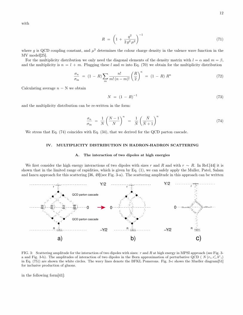
We first consider the high energy interactions of two dipoles with sizes r and R and with r ∼ R. In Ref.[44] it isshown that in the limited range of rapidities, which is given by Eq. (1), we can safely apply the Muller, Patel, Salamand Iancu approach for this scattering [36, 49](see Fig. 3-a). The scattering amplitude in this approach can be written

0

r

R

Y/2

0

−Y/2

QCD parton cascade

QCD parton cascade

r

R

a) b)

0

r

R

Y/2

−Y/2

c)

FIG. 3: Scattering amplitude for the interaction of two dipoles with sizes: r and R at high energy in MPSI approach (see Fig. 3-a and Fig. 3-b). The amplitudes of interaction of two dipoles in the Born approximation of perturbative QCD ( N (ri, r

′i, b”i)

in Eq. (75)) are shown the white circles. The wavy lines denote the BFKL Pomerons. Fig. 3-c shows the Mueller diagram[51]for inclusive production of gluons.

in the following form[41]:

13

N (Y, r,R, b) = −∞∑n=1

(−1)n∫

ρtn

(r1, b

′1, . . . , rn, b

′n;

1

2Y

)ρpn

(r′1, b− b′1 − b′′1 , . . . , rn, b− b′n − b′′n; −1

2Y

)

×n∏i=1

d2 ri

n∏j=1

d2 r′j d2b′jd

2b′′j NBA (ri, r

′i, b′′i ) (75)

where ρtn and ρpn are the parton densities in the target and projectile, respectively. These densities can be calculatedfrom Pn using Eq. (45). NBA is the scattering amplitude of two dipoles in the Born approximation of perturbativeQCD (see Fig. 3). Eq. (75) simply states that we can consider the QCD parton cascade of Eq. (4) generated by thedipole of the size r for the c.m.f. rapidities from 0 to 1

2Y , and the same cascade for the dipole of the size R, for therapidities from 0 to − 1

2Y .Generally speaking, for the dense system of partons at Y = 0 n-dipoles from upper cascade could interact with

m dipoles from the low cascade, with the amplitude Nmn

({ri}, {r′j}

)[41]. In Eq. (75) we assume that the system of

dipoles that has been created at Y = 0 is not very dense. In this case

Nmn

({ri}, {r′j}

)= δn,m

n∏j=1

(−1)n−1

NBA (ri, r′i, b′′i ) (76)

and after integration over {r1} and {r′j}, the scattering amplitude can be reduced to a system of enhanced BFKLPomeron diagrams, which are shown in Fig. 3-b.

The average number of dipoles at Y = 0 are determined by the inclusive cross section, which is given by the diagramof Fig. 3-c and which can be written at y → 0 as follows[52]:

dσ

dy d2pT=

2CFαs(2π)4

1

p2T

∫d2rT e

ipT ·rT∫d2b∇2

T NBFKL

(1

2Y ; r, rT ; b

) ∫d2B∇2

T NBFKL

(y2 = −1

2Y ;R, rT ;B

)(77)

The average number of dipoles that enters the multiplicity distribution of Eq. (34) is equal n = N =∫d2pT(2π)2

dσdy d2pT

/σin ∝ exp (∆BFKL Y )3 only if we assume that σin ∼ Const. Indeed, the enhanced diagrams of

Fig. 3-b lead to the inelastic cross section which is constant at high energy.

B. Hadron - hadron collisions

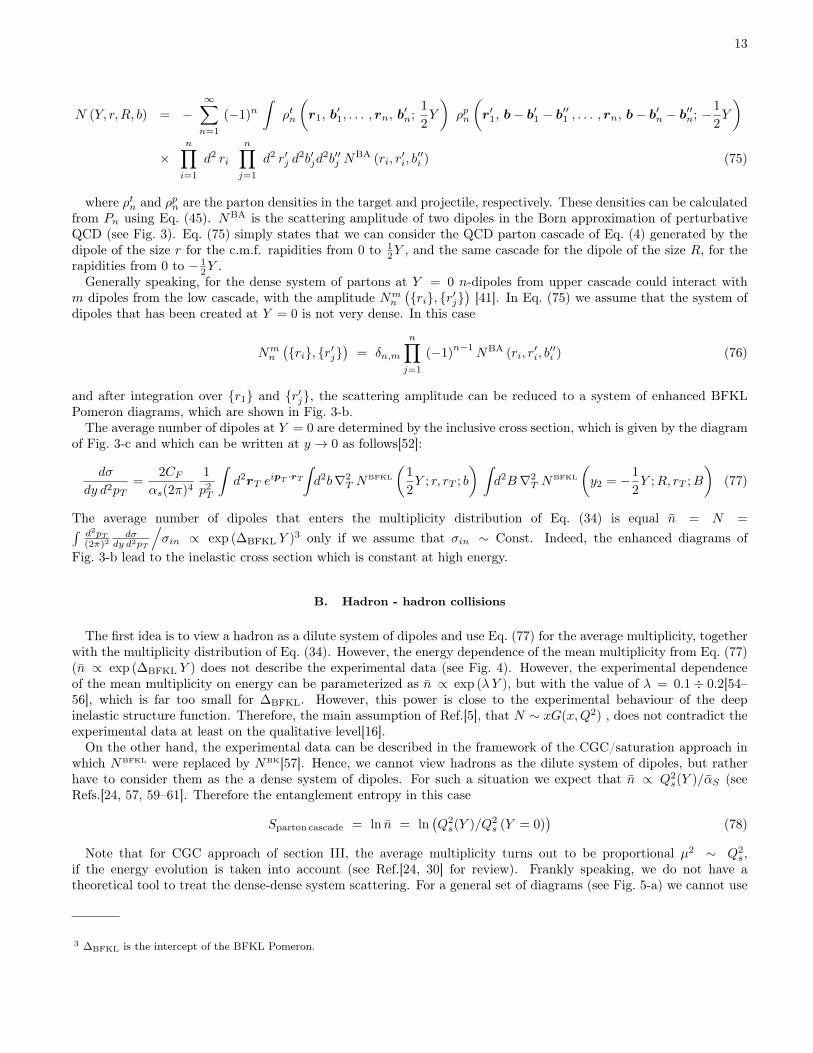
The first idea is to view a hadron as a dilute system of dipoles and use Eq. (77) for the average multiplicity, togetherwith the multiplicity distribution of Eq. (34). However, the energy dependence of the mean multiplicity from Eq. (77)(n ∝ exp (∆BFKL Y ) does not describe the experimental data (see Fig. 4). However, the experimental dependenceof the mean multiplicity on energy can be parameterized as n ∝ exp (λY ), but with the value of λ = 0.1÷ 0.2[54–56], which is far too small for ∆BFKL. However, this power is close to the experimental behaviour of the deepinelastic structure function. Therefore, the main assumption of Ref.[5], that N ∼ xG(x,Q2) , does not contradict theexperimental data at least on the qualitative level[16].

On the other hand, the experimental data can be described in the framework of the CGC/saturation approach inwhich NBFKL were replaced by NBK[57]. Hence, we cannot view hadrons as the dilute system of dipoles, but ratherhave to consider them as the a dense system of dipoles. For such a situation we expect that n ∝ Q2

s(Y )/αS (seeRefs.[24, 57, 59–61]. Therefore the entanglement entropy in this case

Sparton cascade = ln n = ln(Q2s(Y )/Q2

s (Y = 0))

(78)

Note that for CGC approach of section III, the average multiplicity turns out to be proportional µ2 ∼ Q2s,

if the energy evolution is taken into account (see Ref.[24, 30] for review). Frankly speaking, we do not have atheoretical tool to treat the dense-dense system scattering. For a general set of diagrams (see Fig. 5-a) we cannot use

3 ∆BFKL is the intercept of the BFKL Pomeron.

14

[GeV]s210 310

⟩ n

⟨

0

5

10

15

20

25

30 NA22

UA1

UA5

CMS

CMS NSD| < 2.4η |

Gotsman et al.Likhoded et al.Kaidalov and PoghosyanLevin et al.

0

Y/2

−Y/2 hadron

hadron

Fig. 4-a Fig. 4-b

FIG. 4: Fig. 4-a: The comparison of the average multiplicities in proton-proton collisions at |η ≤ 2.4[53] with the theoreticalprediction[54–57]. The figure is taken from Ref.[53]. The CGC prediction is marked by Levin et al. and they are taken fromRef.[57].Fig. 4-b: The Mueller diagram [51] for the inclusive production in CGC/saturation approach. The wavy lines are theBFKL Pomerons. The helical lines denote the gluons. The black blobs stand for the triple Pomeron vertices.

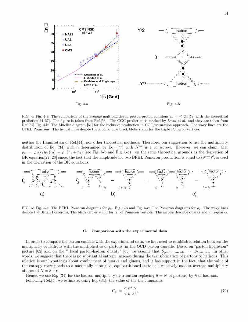
neither the Hamiltotian of Ref.[44], nor other theoretical methods. Therefore, our suggestion to use the multiplicitydistribution of Eq. (34) with n determined by Eq. (77) with NBK is a conjecture. However, we can claim, thatρ2 = ρ1(r1)ρ1(r2) − ρ1 (r1 + r2) (see Fig. 5-b and Fig. 5-c) , on the same theoretical grounds as the derivation ofBK equation[27, 28] since, the fact that the amplitude for two BFKL Pomeron production is equal to (NBK)

2, is usedin the derivation of the BK equations.

n 2

hadron hadronhadronhadron

r + r1 2

_

hadron

r1 r2 r1r + r1 2

_

hadron

__

r2

a) b) c)

__ __

FIG. 5: Fig. 5-a: The BFKL Pomeron diagrams for ρn. Fig. 5-b and Fig. 5-c: The Pomeron diagrams for ρ2. The wavy linesdenote the BFKL Pomerons, The black circles stand for triple Pomeron vertices. The arrows describe quarks and anti-quarks.

C. Comparison with the experimental data

In order to compare the parton cascade with the experimental data, we first need to establish a relation between themultiplicity of hadrons with the multiplicities of partons, in the QCD parton cascade. Based on “parton liberation"picture [62] and on the " local parton-hadron duality" [63] we assume that Sparton cascade = Shadrons. In otherwords, we suggest that there is no substantial entropy increase during the transformation of partons to hadrons. Thisrelation is our hypothesis about confinement of quarks and gluons, and it has support in the fact, that the value ofthe entropy corresponds to a maximally entangled, equipartitioned state at a relatively modest average multiplicityof around N = 3÷ 6.

Hence, we use Eq. (34) for the hadron multiplicity distribution replacing n = N of partons, by n of hadrons.Following Ref.[5], we estimate, using Eq. (34), the value of the the cumulants

Cq =< nq >

< n >q, (79)

15

where < · · · > denotes the average over the distribution in hadron multiplicity n. These quantities can be readilycomputed using Eq. (34)(see Ref.[5]). The result of these estimates are the following:

C2 = 2− 1/n; C3 =6(n− 1)n+ 1

n2;

C4 =(12n(n− 1) + 1)(2n− 1)

n3; C5 =

(n− 1)(120n2(n− 1) + 30n) + 1

n4. (80)

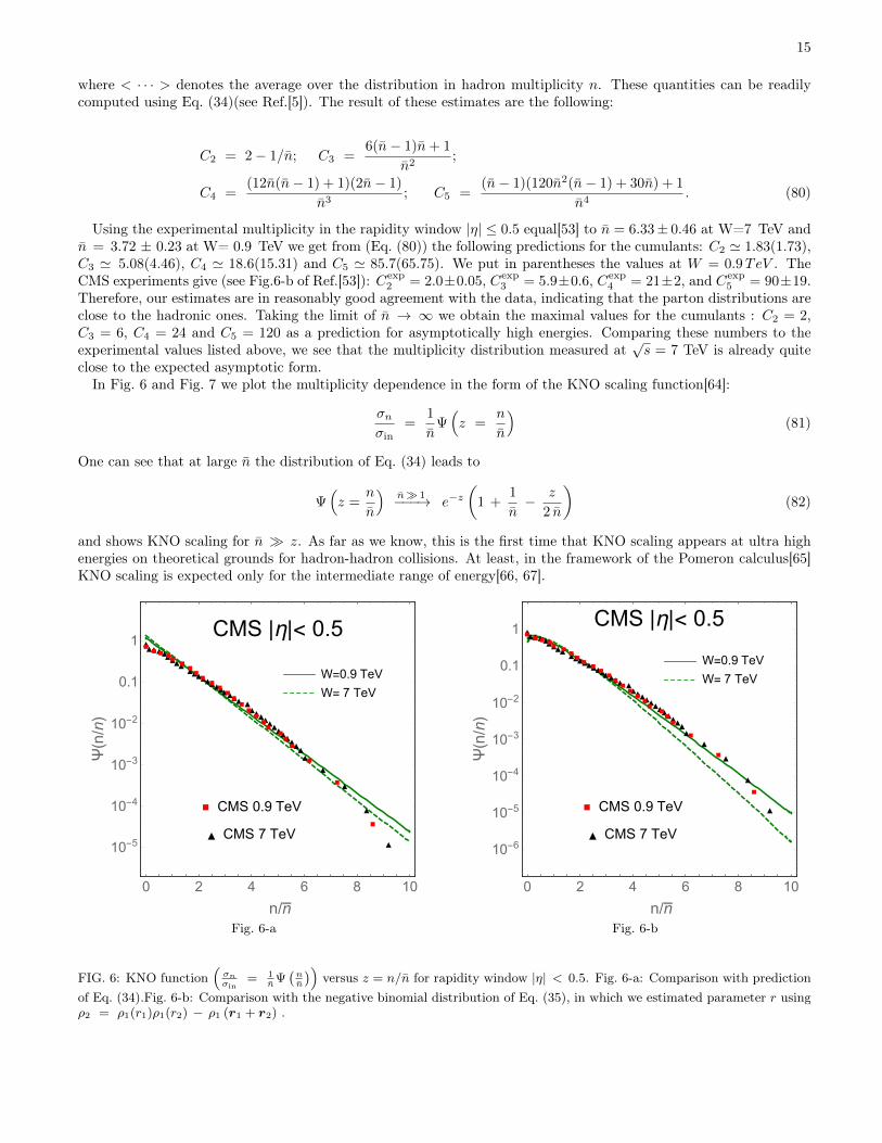
Using the experimental multiplicity in the rapidity window |η| ≤ 0.5 equal[53] to n = 6.33± 0.46 at W=7 TeV andn = 3.72 ± 0.23 at W= 0.9 TeV we get from (Eq. (80)) the following predictions for the cumulants: C2 ' 1.83(1.73),C3 ' 5.08(4.46), C4 ' 18.6(15.31) and C5 ' 85.7(65.75). We put in parentheses the values at W = 0.9TeV . TheCMS experiments give (see Fig.6-b of Ref.[53]): Cexp

2 = 2.0±0.05, Cexp3 = 5.9±0.6, Cexp

4 = 21±2, and Cexp5 = 90±19.

Therefore, our estimates are in reasonably good agreement with the data, indicating that the parton distributions areclose to the hadronic ones. Taking the limit of n → ∞ we obtain the maximal values for the cumulants : C2 = 2,C3 = 6, C4 = 24 and C5 = 120 as a prediction for asymptotically high energies. Comparing these numbers to theexperimental values listed above, we see that the multiplicity distribution measured at

√s = 7 TeV is already quite

close to the expected asymptotic form.In Fig. 6 and Fig. 7 we plot the multiplicity dependence in the form of the KNO scaling function[64]:

σnσin

=1

nΨ(z =

n

n

)(81)

One can see that at large n the distribution of Eq. (34) leads to

Ψ(z =

n

n

)n� 1−−−→ e−z

(1 +

1

n− z

2 n

)(82)

and shows KNO scaling for n � z. As far as we know, this is the first time that KNO scaling appears at ultra highenergies on theoretical grounds for hadron-hadron collisions. At least, in the framework of the Pomeron calculus[65]KNO scaling is expected only for the intermediate range of energy[66, 67].

▲▲▲▲▲▲▲▲▲▲▲▲▲▲▲▲▲▲▲▲▲ ▲

▲▲▲▲▲▲▲▲▲▲▲▲▲

▲

▲

▲

▲

■ ■■■■ ■ ■■■ ■ ■■■■■■■■

■■■

■

■

■

CMS |η|< 0.5

W=0.9 TeV

W= 7 TeV

▲ CMS 7 TeV

■ CMS 0.9 TeV

0 2 4 6 8 10

10-5

10-4

10-3

10-2

0.1

1

n/n

Ψ(n/n)

▲▲▲▲▲▲▲▲▲ ▲▲▲▲▲▲▲▲▲▲▲▲ ▲▲▲▲▲▲▲▲▲▲▲▲▲

▲▲

▲

▲

▲

■ ■■■■ ■ ■■■ ■ ■ ■■■■■■■

■■■

■

■

■

CMS |η|< 0.5

W=0.9 TeV

W= 7 TeV

▲ CMS 7 TeV

■ CMS 0.9 TeV

0 2 4 6 8 10

10-6

10-5

10-4

10-3

10-2

0.1

1

n/n

Ψ(n/n)

Fig. 6-a Fig. 6-b

FIG. 6: KNO function(σnσin

= 1n

Ψ(nn

))versus z = n/n for rapidity window |η| < 0.5. Fig. 6-a: Comparison with prediction

of Eq. (34).Fig. 6-b: Comparison with the negative binomial distribution of Eq. (35), in which we estimated parameter r usingρ2 = ρ1(r1)ρ1(r2) − ρ1 (r1 + r2) .

16

▲

▲▲▲▲▲▲▲▲▲▲▲▲▲▲▲▲▲▲▲▲▲▲▲▲▲▲▲▲▲▲▲▲▲▲▲▲▲▲▲▲▲▲▲▲▲▲▲▲▲▲▲▲▲▲▲▲▲▲▲▲▲▲▲▲▲▲▲▲▲▲▲▲▲▲▲▲▲▲▲▲▲▲▲▲▲▲▲▲▲▲▲▲▲▲▲▲▲▲▲▲▲▲▲▲▲▲▲▲▲▲▲▲▲▲

▲▲

▲

▲

▲

▲

■■■■■■■■■■■■■■■■■■■■■■■■■■■■■■■■■■■■■■■■■■■■■■■

■■■■■■■■■■■■

■

■

■

CMS |η|< 2.4

W=0.9 TeV

W= 7 TeV

▲ CMS 7 TeV

■ CMS 0.9 TeV

0 1 2 3 4 5 6

10-3

10-2

0.1

1

n/n

Ψ(n/n)

▲

▲▲▲▲▲▲▲▲▲▲▲▲▲▲▲▲▲▲▲▲▲▲▲▲▲▲▲▲▲▲▲▲▲▲▲▲▲▲▲▲▲▲▲▲▲▲▲▲▲▲▲▲▲▲▲▲▲▲▲▲▲▲▲▲▲▲▲▲▲▲▲▲▲▲▲▲▲▲▲▲▲▲▲▲▲▲▲▲▲▲▲▲▲▲▲▲▲▲▲▲▲▲▲▲▲▲▲▲▲▲▲▲▲▲

▲▲

▲

▲

▲

▲

■■■■■■■■■■■■■■■■■■■■■■■■■■■■■■■■■■■■■■■■■■■■■■■

■■■■■■■■■■■■

■

■

■

CMS |η|< 2.4

W=0.9 TeV

W= 7 TeV

▲ CMS 7 TeV

■ CMS 0.9 TeV

0 1 2 3 4 5 6

10-3

10-2

0.1

1

n/n

Ψ(n/n)

Fig. 7-a Fig. 7-b

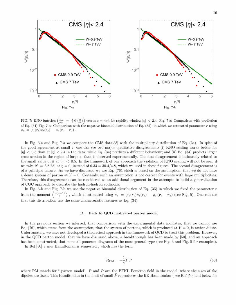
FIG. 7: KNO function(σnσin

= 1n

Ψ(nn

))versus z = n/n for rapidity window |η| < 2.4. Fig. 7-a: Comparison with prediction

of Eq. (34).Fig. 7-b: Comparison with the negative binomial distribution of Eq. (35), in which we estimated parameter r usingρ2 = ρ1(r1)ρ1(r2) − ρ1 (r1 + r2) .

In Fig. 6-a and Fig. 7-a we compare the CMS data[53] with the multiplicity distribution of Eq. (34). In spite ofthe good agreement at small z, one can see two major qualitative disagreements:(i) KNO scaling works better for|η| < 0.5 than at |η| < 2.4 in the data, while Eq. (34) predicts a different behaviour; and (ii) Eq. (34) predicts largercross section in the region of large z, than is observed experimentally. The first disagreement is intimately related tothe small value of n at |η| < 0.5. In the framework of our approach the violation of KNO scaling will not be seen ifwe take N = 5.8[68] at η = 0, instead of 6.33 = 30.4/4.8, which we used in these figures. The second disagreement isof a principle nature. As we have discussed we use Eq. (76),which is based on the assumption, that we do not havea dense system of parton at Y = 0. Certainly, such an assumption is not correct for events with large multiplicities.Therefore, this disagreement can be considered as an additional argument in the attempts to build a generalizationof CGC approach to describe the hadron-hadron collisions.

In Fig. 6-b and Fig. 7-b we use the negative binomial distribution of Eq. (35) in which we fixed the parameter rfrom the moment

⟨n(n−1)

2

⟩, which is estimated using ρ2 = ρ1(r1)ρ1(r2) − ρ1 (r1 + r2) (see Fig. 5). One can see

that this distribution has the same characteristic features as Eq. (34).

D. Back to QCD motivated parton model

In the previous section we inferred, that comparison with the experimental data indicates, that we cannot useEq. (76), which stems from the assumption, that the system of partons, which is produced at Y = 0, is rather dilute.Unfortunately, we have not developed a theoretical approach in the framework of QCD to treat this problem. However,in the QCD parton model, that we have discussed above, a breakthrough has been made by [50], and an approachhas been constructed, that sums all pomeron diagrams of the most general type (see Fig. 3 and Fig. 5 for examples).

In Ref.[50] a new Hamiltonian is suggested , which has the form

HPM = − 1

γP P (83)

where PM stands for “ parton model”. P and P are the BFKL Pomeron field in the model, where the sizes of thedipoles are fixed. This Hamiltonian in the limit of small P reproduces the BK Hamiltonian ( see Ref.[50] and below for

17

details). This condition is the most important one for fixing the form of HPM. The second of such conditions is thatthis Hamiltonian satisfies both t and s channel unitarity. γ in Eq. (83) has the physical meaning of the dipole-dipolescattering amplitude in the Born approximation of perturbative QCD and, being such, it is naturally small and oforder αS .

The most important ingredient of this approach is the generalization of the commutation relation, which has theform: (

1 − P)(

1 − P)

= (1− γ)(

1 − P)(

1 − P)

(84)

Eq. (84) gives the correct factor (1− γ)n that includes all multiple scattering corrections, while all the dipoles remainintact, and can subsequently scatter on an additional projectile or on target dipoles. For small γ, and in the regimewhere P and P are small themselves, we obtain

[P, P ] = −γ + ... (85)

consistent with our original expression. One can see that these commutation relations take into account the interactionof one dipole with many other partons and, therefore, we are going beyond the approximation, which is given byEq. (76). Concluding this brief outline of this approach, we see, that for the first time we have a simple theory inwhich we can describe the interactions of dilute-dilute parton system scattering, as well as dilute-dense and dense-densesystem interactions.

For HPM the cascade equation takes the form (see Eq. 5.8 of Ref.[50]):

dPn (Y )

dY= −∆

γ

(1−

(1 − γ

)n )Pn (Y ) +

∆

γ

(1− (1 − γ)

n−1)Pn−1 (Y.) (86)

For small n (γ n < 1) one can see, that Eq. (86) reduces to Eq. (39). Hence, for such small n we have the multiplicitydistribution of Eq. (41) with < n >= e∆Y . However, at large n Eq. (86) has the form

dPn (Y )

dY= −∆

γPn (Y ) +

∆

γPn−1 (Y ) (87)

We will show below that this equation gives the Poisson distribution with < n >= ∆γ Y . Therefore, as we have

guessed the interaction of one dipole with many dipoles at Y = 0 in Fig. 3 would lead to far fewer multiplicities thanEq. (41). Using Laplace transform of Eq. (27) and following the pattern, described in section II-C, we obtain thesolution in ω-representation:

Pn (ω) =1

ω1

n∏m=1

ωmω + ωm

(88)

where ωm = ∆γ

(1− (1 − γ)

m).

We have not found an elegant form for the inverse Laplace transform, but we can see the main qualitative featuresof this solution, assuming that for n < n0 with γ n0 ≈ 1 we have ωm = m∆, but for n > n0 ωm = ∆

γ . In thisapproach we obtain:

n < n0 Pn (Y ) = e−∆Y(

1 − e−∆Y)n−1

; (89a)

n > n0 Pn (Y ) =

∫ Y

dY ′e−∆ (Y−Y ′)(

1 − e−∆ (Y−Y ′))n0−1

e−∆γ Y

′

(∆γ Y′)n−n0

(n− n0)!︸ ︷︷ ︸Poisson distribution

; (89b)

The Poisson distribution in Eq. (89b) is the inverse Laplace transform of(∆γ

)n−n0

(ω + ∆

γ

)n−n0+1 (90)

18

Eq.33

Eq.88

0 2 4 6 8 10

1

2

5

10

20

50

Y

<n>

Eq.33

Eq.88

2 4 6 8 10

1

10

100

1000

Y

<n(n-1>/2 Eq.33

Eq.88

0 20 40 60 80

10-20

10-15

10-10

10-5

1

n

σn/σin

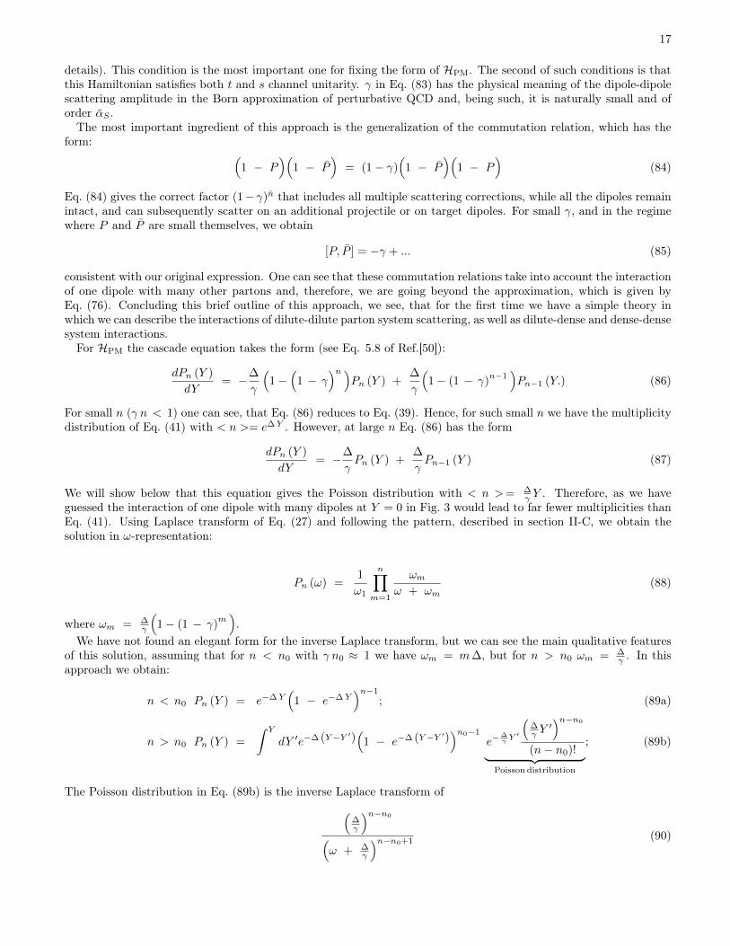
Fig. 8-a Fig. 8-b Fig. 8-c

FIG. 8: Comparison of the multiplicity distribution, given by Eq. (34) with the modified distribution of Eq. (89a) andEq. (89b).

In Fig. 8 we compare this multiplicity distribution with Eq. (34). One can see that at large multiplicities themodified distribution of Eq. (89a) and Eq. (89b) lead to the suppression of the parton emission, as we expected. Ofcourse, this modified distribution is very approximate, and can only be used to clarify the qualitative features of theinteraction of the partons in the exact approach.

To illustrate that the parton cascade of Eq. (86) is able to describe the experimental data. We calculate the firsttwo P1 and P2, taking integral over ω in Eq. (27):

P1 (Y ) = e∆Y ; P2 (Y ) =ω2

ω2 − ω1e−ω1 Y

(1 − e−(ω2−ω1)Y

)(91)

where ω2 − ω1 = ∆ − γ∆ < ∆. P2 in our notation with N = e∆Y can be re-written in the form:

P2 =1

N

(1 −

(1

N

)1−γ)

(92)

Assuming that the multiplicity distribution has the form:

Pn =1

N

(1 −

(1

N

)1−γ)n−1

(93)

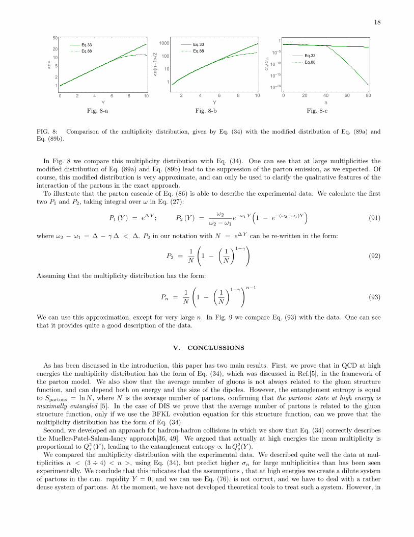
We can use this approximation, except for very large n. In Fig. 9 we compare Eq. (93) with the data. One can seethat it provides quite a good description of the data.

V. CONCLUSSIONS

As has been discussed in the introduction, this paper has two main results. First, we prove that in QCD at highenergies the multiplicity distribution has the form of Eq. (34), which was discussed in Ref.[5], in the framework ofthe parton model. We also show that the average number of gluons is not always related to the gluon structurefunction, and can depend both on energy and the size of the dipoles. However, the entanglement entropy is equalto Spartons = lnN , where N is the average number of partons, confirming that the partonic state at high energy ismaximally entangled [5]. In the case of DIS we prove that the average number of partons is related to the gluonstructure function, only if we use the BFKL evolution equation for this structure function, can we prove that themultiplicity distribution has the form of Eq. (34).

Second, we developed an approach for hadron-hadron collisions in which we show that Eq. (34) correctly describesthe Mueller-Patel-Salam-Iancy approach[36, 49]. We argued that actually at high energies the mean multiplicity isproportional to Q2

s (Y ), leading to the entanglement entropy ∝ lnQ2s(Y ).

We compared the multiplicity distribution with the experimental data. We described quite well the data at mul-tiplicities n < (3 ÷ 4) < n >, using Eq. (34), but predict higher σn for large multiplicities than has been seenexperimentally. We conclude that this indicates that the assumptions , that at high energies we create a dilute systemof partons in the c.m. rapidity Y = 0, and we can use Eq. (76), is not correct, and we have to deal with a ratherdense system of partons. At the moment, we have not developed theoretical tools to treat such a system. However, in

19

▲

▲▲▲▲▲▲▲▲▲▲▲▲▲▲▲▲▲▲▲▲▲▲▲▲▲▲▲▲▲▲▲▲▲▲▲▲▲▲▲▲▲▲▲▲▲▲▲▲▲▲▲▲▲▲▲▲▲▲▲▲▲▲▲▲▲▲▲▲▲▲▲▲▲▲▲▲▲▲▲▲▲▲▲▲▲▲▲▲▲▲▲▲▲▲▲▲▲▲▲▲▲▲▲▲▲▲▲▲▲▲▲▲▲▲

▲▲

▲▲

▲

▲

▲

CMS W=7TeV, |η|< 2.4

Mod. Dist.

Distribution

▲ CMS 7 TeV

0 1 2 3 4 5 6

10-3

10-2

0.1

1

n/n

Ψ(n/n)

FIG. 9: KNO function(σnσin

= 1n

Ψ(nn

))versus z = n/n for rapidity window |η| < 2.4. Comparison between multiplicity

distribution of Eq. (34) and modified distribution of Eq. (93), which was used for z > 3.5., γ is equal to 0.15. The data is takenfrom Ref.[53].

Ref.[50], an approach was developed for the parton model, which allow us to theoretically treat such dense system ofpartons. We show that in this approach the production of a system of partons with large multiplicities is suppressedin comparison with Eq. (34), and we are able to describe the experimental data.

VI. ACKNOWLEDGEMENTS

We thank our colleagues at Tel Aviv university and UTFSM for encouraging discussions. This research was sup-ported by ANID PIA/APOYO AFB180002 (Chile) and Fondecyt (Chile) grants 1180118.

∗ Electronic address: gotsman@post.tau.ac.il† Electronic address: leving@tauex.tau.ac.il, eugeny.levin@usm.cl

[1] K. Kutak, “Gluon saturation and entropy production in proton?proton collisions,” Phys. Lett. B 705 (2011), 217-221doi:10.1016/j.physletb.2011.09.113 [arXiv:1103.3654 [hep-ph]].

[2] R. Peschanski, “Dynamical entropy of dense QCD states,” Phys. Rev. D 87 (2013) no.3, 034042doi:10.1103/PhysRevD.87.034042 [arXiv:1211.6911 [hep-ph]].

[3] A. Kovner and M. Lublinsky, “Entanglement entropy and entropy production in the Color Glass Condensate framework,”Phys. Rev. D 92 (2015) no.3, 034016 doi:10.1103/PhysRevD.92.034016 [arXiv:1506.05394 [hep-ph]].

[4] R. Peschanski and S. Seki, “Entanglement Entropy of Scattering Particles,” Phys. Lett. B 758 (2016), 89-92doi:10.1016/j.physletb.2016.04.063 [arXiv:1602.00720 [hep-th]].

[5] D. E. Kharzeev and E. M. Levin, “Deep inelastic scattering as a probe of entanglement,” Phys. Rev. D 95 (2017) no.11,114008 doi:10.1103/PhysRevD.95.114008 [arXiv:1702.03489 [hep-ph]].

[6] O. Baker and D. Kharzeev, “Thermal radiation and entanglement in proton-proton collisions at energies available at theCERN Large Hadron Collider,” Phys. Rev. D 98 (2018) no.5, 054007 doi:10.1103/PhysRevD.98.054007 [arXiv:1712.04558[hep-ph]].

[7] J. Berges, S. Floerchinger and R. Venugopalan, “Dynamics of entanglement in expanding quantum fields,” JHEP 04 (2018),145 doi:10.1007/JHEP04(2018)145 [arXiv:1712.09362 [hep-th]].

[8] Y. Hagiwara, Y. Hatta, B. W. Xiao and F. Yuan, “Classical and quantum entropy of parton distributions,” Phys. Rev. D97 (2018) no.9, 094029 doi:10.1103/PhysRevD.97.094029 [arXiv:1801.00087 [hep-ph]].

[9] N. Armesto, F. Dominguez, A. Kovner, M. Lublinsky and V. Skokov, “The Color Glass Condensate density matrix:Lindblad evolution, entanglement entropy and Wigner functional,” JHEP 05 (2019), 025 doi:10.1007/JHEP05(2019)025

20

[arXiv:1901.08080 [hep-ph]].[10] E. Gotsman and E. Levin, “Thermal radiation and inclusive production in the CGC/saturation approach at high energies,”

Eur. Phys. J. C 79 (2019) no.5, 415 doi:10.1140/epjc/s10052-019-6923-0 [arXiv:1902.07923 [hep-ph]].[11] E. Gotsman and E. Levin, “Thermal radiation and inclusive production in the Kharzeev-Levin-Nardi model for ion-ion

collisions,” Phys. Rev. D 100 (2019) no.3, 034013 doi:10.1103/PhysRevD.100.034013 [arXiv:1905.05167 [hep-ph]].[12] A. Kovner, M. Lublinsky and M. Serino, “Entanglement entropy, entropy production and time evolution in high energy

QCD,” Phys. Lett. B 792 (2019), 4-15 doi:10.1016/j.physletb.2018.10.043 [arXiv:1806.01089 [hep-ph]].[13] D. Neill and W. J. Waalewijn, “Entropy of a Jet,” Phys. Rev. Lett. 123 (2019) no.14, 142001

doi:10.1103/PhysRevLett.123.142001 [arXiv:1811.01021 [hep-ph]].[14] Y. Liu and I. Zahed, “Entanglement in Regge scattering using the AdS/CFT correspondence,” Phys. Rev. D 100 (2019)

no.4, 046005 doi:10.1103/PhysRevD.100.046005 [arXiv:1803.09157 [hep-ph]].[15] X. Feal, C. Pajares and R. Vazquez, “Thermal behavior and entanglement in Pb-Pb and p-p collisions,” Phys. Rev. C 99

(2019) no.1, 015205 doi:10.1103/PhysRevC.99.015205 [arXiv:1805.12444 [hep-ph]].[16] Z. Tu, D. E. Kharzeev and T. Ullrich, “Einstein-Podolsky-Rosen Paradox and Quantum Entanglement at Subnucleonic

Scales,” Phys. Rev. Lett. 124 (2020) no.6, 062001 doi:10.1103/PhysRevLett.124.062001 [arXiv:1904.11974 [hep-ph]].[17] H. Duan, C. Akkaya, A. Kovner and V. V. Skokov,“Entanglement, partial set of measurements, and diagonality of the density

matrix in the parton model,” Phys. Rev. D 101 (2020) no.3, 036017 doi:10.1103/PhysRevD.101.036017 [arXiv:2001.01726[hep-ph]].

[18] J. D. Bjorken, “Asymptotic Sum Rules at Infinite Momentum,” Phys. Rev. 179, 1547 (1969). doi:10.1103/PhysRev.179.1547[19] R.P. Feynman, “Very high-energy collisions of hadrons,” Phys. Rev. Lett. 23, 1415 (1969). “Photon-hadron interactions,”

Reading 1972. Photon-Hadron Interactions, Reading, 1972.[20] J.D. Bjorken and E.A. Paschos,“Inelastic Electron-Proton and γ -Proton Scattering and the Structure of the Nucleon,"

Phys. Rev. 185, 1975(1969).[21] V.N. Gribov, “Inelastic processes at super high-energies and the problem of nuclear cross-sections,” Sov. J. Nucl. Phys. 9,

369 (1969) [Yad. Fiz. 9, 640 (1969)]; “Space-time description of hadron interactions at high-energies,” Proc. ITEP Schoolon Elementary particle physics, v.1, p.65 (1973); hep-ph/0006158.

[22] V. N. Gribov, B. L. Ioffe and I. Y. Pomeranchuk, “What is the range of interactions at high-energies,” Sov. J. Nucl. Phys.2, 549 (1966) [Yad. Fiz. 2, 768 (1965)].

[23] B. L. Ioffe, “Space-time picture of photon and neutrino scattering and electroproduction cross-section asymptotics,” Phys.Lett. 30B, 123 (1969). doi:10.1016/0370-2693(69)90415-8

[24] Yuri V. Kovchegov and Eugene Levin, “ Quantum Chromodynamics at High Energies", Cambridge Monographs on ParticlePhysics, Nuclear Physics and Cosmology, Cambridge University Press, 2012 .

[25] L. McLerran and R. Venugopalan, “Computing quark and gluon distribution functions for very large nuclei", Phys. Rev.D49 (1994) 2233, “Gluon distribution functions for very large nuclei at small transverse momentum", Phys. Rev. D49(1994), 3352; ‘Green?s function in the color field of a large nucleus", D50 (1994) 2225; “ Fock space distributions, structurefunctions, higher twists, and small x" , D59 (1999) 09400.

[26] A. H. Mueller, “Soft Gluons In The Infinite Momentum Wave Function And The BFKL Pomeron,” Nucl. Phys. B 415,373 (1994); “Unitarity and the BFKL pomeron,” Nucl. Phys. B 437 (1995) 107 [arXiv:hep-ph/9408245].

[27] I. Balitsky, “Operator expansion for high-energy scattering", [arXiv:hep-ph/9509348]; “Factorization and high-energy ef-fective action", Phys. Rev. D60, 014020 (1999) [arXiv:hep-ph/9812311].

[28] Y. V. Kovchegov, “ Small-x F2 structure function of a nucleus including multiple Pomeron exchanges"’ Phys. Rev. D60,034008 (1999), [arXiv:hep-ph/9901281].

[29] J. Jalilian-Marian, A. Kovner, A. Leonidov, and H. Weigert, “The BFKL equation from the Wilson renormalization group", Nucl. Phys. B504 (1997) 415–431, [ arXiv:hep-ph/9701284]; J. Jalilian-Marian, A. Kovner, A. Leonidov, and H. Weigert,“The Wilson renormalization group for low x physics: Towards the high density regime" , Phys.Rev. D59 (1998) 014014,[arXiv:hep-ph/9706377 [hep-ph]]; A. Kovner, J. G. Milhano, and H. Weigert, “Relating different approaches to nonlinearQCD evolution at finite gluon density" , Phys. Rev. D62 (2000) 114005, [ arXiv:hep-ph/0004014]; E. Iancu, A. Leonidov,and L. D. McLerran, Nonlinear gluon evolution in the color glass condensate. I" ,Nucl. Phys. A692 (2001) 583–645, [arXiv:hep-ph/0011241]; E. Iancu, A. Leonidov, and L. D. McLerran, “The renormalization group equation for the colorglass condensate" , Phys. Lett. B510 (2001) 133–144, [ arXiv:hep-ph/0102009]; E. Ferreiro, E. Iancu, A. Leonidov, andL. McLerran, “Nonlinear gluon evolution in the color glass condensate. II" , Nucl. Phys. A703 (2002) 489–538, [ arXiv:hep-ph/0109115]; H. Weigert, Unitarity at small Bjorken x, Nucl. Phys. A703, 823 (2002), [arXiv:hep-ph/0004044].

[30] F. Gelis, E. Iancu, J. Jalilian-Marian and R. Venugopalan, “The Color Glass Condensate,” Ann. Rev. Nucl. Part. Sci. 60(2010), 463-489 doi:10.1146/annurev.nucl.010909.083629 [arXiv:1002.0333 [hep-ph]].

[31] V. S. Fadin, E. A. Kuraev and L. N. Lipatov, “On the pomeranchuk singularity in asymptotically free theories", Phys.Lett. B60, 50 (1975); E. A. Kuraev, L. N. Lipatov and V. S. Fadin, “The Pomeranchuk Singularity in Nonabelian GaugeTheories" Sov. Phys. JETP 45, 199 (1977), [Zh. Eksp. Teor. Fiz.72,377(1977)]; “The Pomeranchuk Singularity in QuantumChromodynamics,” I. I. Balitsky and L. N. Lipatov, Sov. J. Nucl. Phys. 28, 822 (1978), [Yad. Fiz.28,1597(1978)].

[32] L. N. Lipatov, “The Bare Pomeron in Quantum Chromodynamics,” Sov. Phys. JETP 63, 904 (1986) [Zh. Eksp. Teor. Fiz.90, 1536 (1986)].

[33] L. V. Gribov, E. M. Levin and M. G. Ryskin, “Semihard Processes in QCD,” Phys. Rept. 100, 1 (1983). doi:10.1016/0370-1573(83)90022-4

[34] E. M. Levin and M. G. Ryskin, “High-energy hadron collisions in QCD,” Phys. Rept. 189, 267 (1990).[35] A. H. Mueller and J. Qiu, “ Gluon recombination and shadowing at small values of x", Nucl. Phys. B268 (1986) 427.

21

[36] A. H. Mueller and B. Patel, “Single and double BFKL pomeron exchange and a dipole picture of high-energy hard processes",Nucl. Phys. B425 (1994) 471.

[37] J. Bartels, M. Braun and G. Vacca, “Pomeron vertices in perturbative QCD in diffractive scattering,” Eur. Phys. J. C40 (2005), 419-433 doi:10.1140/epjc/s2005-02152-x [arXiv:hep-ph/0412218 [hep-ph]]; J. Bartels and C. Ewerz, “Unitaritycorrections in high-energy QCD,” JHEP 09 (1999), 026 doi:10.1088/1126-6708/1999/09/026 [arXiv:hep-ph/9908454 [hep-ph]]; J. Bartels and M. Wusthoff, “The Triple Regge limit of diffractive dissociation in deep inelastic scattering,” Z. Phys.C 66 (1995), 157-180 doi:10.1007/BF01496591; J. Bartels, “Unitarity corrections to the Lipatov pomeron and the four gluonoperator in deep inelastic scattering in QCD,” Z. Phys. C 60 (1993), 471-488 doi:10.1007/BF01560045

[38] M. Braun, “Conformal invariant pomeron interaction in the perurbative QCD with large Nc,” Phys. Lett. B 632 (2006),297-304 doi:10.1016/j.physletb.2005.10.054 [arXiv:hep-ph/0512057 [hep-ph]]; “Nucleus nucleus interaction in the per-turbative QCD,” Eur. Phys. J. C 33 (2004), 113-122 doi:10.1140/epjc/s2003-01565-9 [arXiv:hep-ph/0309293 [hep-ph]];“Nucleus-nucleus scattering in perturbative QCD with Nc → infinity,” Phys. Lett. B 483 (2000), 115-123 doi:10.1016/S0370-2693(00)00571-2 [arXiv:hep-ph/0003004 [hep-ph]]; “Structure function of the nucleus in the perturbative QCD with Nc →infinity (BFKL pomeron fan diagrams),” Eur. Phys. J. C 16 (2000), 337-347 doi:10.1007/s100520050026 [arXiv:hep-ph/0001268 [hep-ph]]; “The system of four reggeized gluons and the three-pomeron vertex in the high colour limit" Eur.Phys. J. C6, 321 (1999) [arXiv:hep-ph/9706373]; M. Braun and G. Vacca, “Triple pomeron vertex in the limit Nc →infinity,” Eur. Phys. J. C 6 (1999), 147-157 doi:10.1007/s100520050328 [arXiv:hep-ph/9711486 [hep-ph]].

[39] Y. V. Kovchegov and E. Levin, “Diffractive dissociation including multiple pomeron exchanges in high parton density QCD,”Nucl. Phys. B 577 (2000), 221-239 doi:10.1016/S0550-3213(00)00125-5 [arXiv:hep-ph/9911523 [hep-ph]].

[40] E. Levin and M. Lublinsky, “Towards a symmetric approach to high energy evolution: Generating functional with Pomeronloops,” Nucl. Phys. A 763 (2005) 172 [arXiv:hep-ph/0501173].

[41] E. Levin and M. Lublinsky, “Balitsky’s hierarchy from Mueller’s dipole model and more about target correlations,” Phys.Lett. B 607 (2005) 131 [arXiv:hep-ph/0411121]; “A linear evolution for non-linear dynamics and correlations in realisticnuclei,” Nucl. Phys. A 730 (2004) 191 [arXiv:hep-ph/0308279].

[42] E. Levin, J. Miller and A. Prygarin, “Summing Pomeron loops in the dipole approach,” Nucl. Phys. A806 (2008) 245,[arXiv:0706.2944 [hep-ph]].

[43] T. Altinoluk, C. Contreras, A. Kovner, E. Levin, M. Lublinsky and A. Shulkim, “QCD reggeon calculus from JIMWLK Evo-lution,” Int. J. Mod. Phys. Conf. Ser. 25 (2014) 1460025; T. Altinoluk, N. Armesto, A. Kovner, E. Levin and M. Lublinsky,“KLWMIJ Reggeon field theory beyond the large Nc limit,” JHEP 1408 (2014) 007.

[44] T. Altinoluk, A. Kovner, E. Levin and M. Lublinsky, “Reggeon Field Theory for Large Pomeron Loops,” JHEP 1404 (2014)075 [arXiv:1401.7431 [hep-ph]].; T. Altinoluk, C. Contreras, A. Kovner, E. Levin, M. Lublinsky and A. Shulkin, “QCDReggeon Calculus From KLWMIJ/JIMWLK Evolution: Vertices, Reggeization and All,” JHEP 1309 (2013) 115.

[45] E. Levin, “Dipole-dipole scattering in CGC/saturation approach at high energy: summing Pomeron loops,’ JHEP 1311(2013) 039 [arXiv:1308.5052 [hep-ph]].

[46] A. Kovner, M. Lublinsky and U. Wiedemann, “From bubbles to foam: Dilute to dense evolution of hadronic wave functionat high energy,” JHEP 06 (2007), 075 doi:10.1088/1126-6708/2007/06/075 [arXiv:0705.1713 [hep-ph]].

[47] T. Altinoluk, A. Kovner, M. Lublinsky and J. Peressutti, “QCD Reggeon Field Theory for every day: Pomeron loopsincluded,” JHEP 03 (2009), 109 doi:10.1088/1126-6708/2009/03/109 [arXiv:0901.2559 [hep-ph]].

[48] I. Gradstein and I. Ryzhik, Table of Integrals, Series, and Products, Fifth Edition, Academic Press, London, 1994.[49] A. H. Mueller and G. Salam, “Large multiplicity fluctuations and saturation effects in onium collisions,” Nucl. Phys.

B 475 (1996), 293-320 doi:10.1016/0550-3213(96)00336-7 [arXiv:hep-ph/9605302 [hep-ph]]; G. Salam, “Studies of uni-tarity at small x using the dipole formulation,” Nucl. Phys. B 461 (1996), 512-538 doi:10.1016/0550-3213(95)00658-3 [arXiv:hep-ph/9509353 [hep-ph]]; E. Iancu and A. Mueller, “Rare fluctuations and the high-energy limit of the Smatrix in QCD,” Nucl. Phys. A 730 (2004), 494-513 doi:10.1016/j.nuclphysa.2003.10.019 [arXiv:hep-ph/0309276 [hep-ph]]; “From color glass to color dipoles in high-energy onium onium scattering,” Nucl. Phys. A 730 (2004), 460-493doi:10.1016/j.nuclphysa.2003.10.017 [arXiv:hep-ph/0308315 [hep-ph]].

[50] A. Kovner, E. Levin and M. Lublinsky, “QCD unitarity constraints on Reggeon Field Theory,” JHEP 08 (2016), 031doi:10.1007/JHEP08(2016)031 [arXiv:1605.03251 [hep-ph]].

[51] A. H. Mueller, “O(2,1) analysis of single particle spectra at high energy,” Phys. Rev. D2 (1970) 2963.[52] Y. V. Kovchegov and K. Tuchin, “Inclusive gluon production in DIS at high parton density,” Phys. Rev. D65 (2002) 074026

[arXiv:hep-ph/0111362].[53] V. Khachatryan et al. [CMS], “Charged Particle Multiplicities in pp Interactions at

√s = 0.9, 2.36, and 7 TeV,” JHEP 01

(2011), 079 doi:10.1007/JHEP01(2011)079 [arXiv:1011.5531 [hep-ex]].[54] E. Gotsman, A. Kormilitzin, E. Levin and U. Maor, “QCD motivated approach to soft interactions at high energies:

nucleus-nucleus and hadron-nucleus collisions,” Nucl. Phys. A 842 (2010), 82-101 doi:10.1016/j.nuclphysa.2010.04.016[arXiv:0912.4689 [hep-ph]].

[55] A. Likhoded, A. Luchinsky and A. Novoselov, “Light hadron production in inclusive pp-scattering at LHC,” Phys. Rev. D82 (2010), 114006 doi:10.1103/PhysRevD.82.114006 [arXiv:1005.1827 [hep-ph]].

[56] A. Kaidalov and M. Poghosyan, “Predictions of Quark-Gluon String Model for pp at LHC,” Eur. Phys. J. C 67 (2010),397-404 doi:10.1140/epjc/s10052-010-1301-y [arXiv:0910.2050 [hep-ph]].

[57] E. Levin and A. H. Rezaeian, “Gluon saturation and inclusive hadron production at LHC,” Phys. Rev. D 82 (2010), 014022doi:10.1103/PhysRevD.82.014022 [arXiv:1005.0631 [hep-ph]].

[58] D. Kharzeev and M. Nardi, “Hadron production in nuclear collisions at RHIC and high density QCD,” Phys. Lett. B 507,121 (2001) [nucl-th/0012025].

22

[59] . D. Kharzeev and E. Levin, ‘ ‘Manifestations of high density QCD in the first RHIC data,” Phys. Lett. B 523 (2001) 79,[nucl-th/0108006]; D. Kharzeev, E. Levin and M. Nardi, “The Onset of classical QCD dynamics in relativistic heavy ioncollisions,” Phys. Rev. C 71 (2005) 054903, [hep-ph/0111315]; “Hadron multiplicities at the LHC,” J. Phys. G 35 (2008)no.5, 054001.38 [arXiv:0707.0811 [hep-ph]].

[60] A. Dumitru, D. E. Kharzeev, E. M. Levin and Y. Nara, “ “Gluon Saturation in pA Collisions at the LHC: KLN ModelPredictions For Hadron Multiplicities,” Phys. Rev. C 85 (2012) 044920 [arXiv:1111.3031 [hep-ph]]

[61] T. Lappi, “Energy dependence of the saturation scale and the charged multiplicity in pp and AA collisions,” Eur. Phys. J. C71, 1699 (2011) [arXiv:1104.3725 [hep-ph]].

[62] A. H. Mueller, “Toward equilibration in the early stages after a high-energy heavy ion collision,” Nucl. Phys. B 572 (2000),227-240 doi:10.1016/S0550-3213(99)00502-7 [arXiv:hep-ph/9906322 [hep-ph]].

[63] Y. L. Dokshitzer, V. A. Khoze, S. I. Troian and A. H. Mueller, “QCD Coherence in High-Energy Reactions,” Rev. Mod.Phys. 60, 373 (1988). doi:10.1103/RevModPhys.60.373

[64] Z. Koba, H. B. Nielsen and P. Olesen, “Scaling of multiplicity distributions in high-energy hadron collisions,” Nucl. Phys.B 40 (1972), 317-334 doi:10.1016/0550-3213(72)90551-2

[65] V. N. Gribov, “A reggeon diagram technique,” Sov. Phys. JETP 26 (1967) 414 [ Zh. Eksp. Teor. Fiz. 53 (1967) 654].[66] V. Abramovskii and O. Kancheli, “Regge branching and distribution of hadron multiplicity at high energies,” Pisma Zh.

Eksp. Teor. Fiz. 15 (1972), 559-563.[67] S. G. Matinyan and W. Walker, “Multiplicity distribution and mechanisms of the high-energy hadron collisions,” Phys. Rev.

D 59 (1999), 034022 doi:10.1103/PhysRevD.59.034022 [arXiv:hep-ph/9801219 [hep-ph]] and reference therein.[68] C. Patrignani et al. (Particle Data Group), Chin. Phys. C, 40, 100001 (2016).