Hierarchical surface reconstruction frommulti-resolution point samples

Ronny Klowsky, Patrick Mucke, and Michael Goesele

TU Darmstadt

Abstract. Robust surface reconstruction from sample points is a chal-lenging problem, especially for real-world input data. We present a newhierarchical surface reconstruction based on volumetric graph-cuts thatincorporates significant improvements over existing methods. One keyaspect of our method is, that we exploit the footprint information whichis inherent to each sample point and describes the underlying surfaceregion represented by that sample. We interpret each sample as a votefor a region in space where the size of the region depends on the foot-print size. In our method, sample points with large footprints do notdestroy the fine detail captured by sample points with small footprints.The footprints also steer the inhomogeneous volumetric resolution usedlocally in order to capture fine detail even in large-scale scenes. Simi-lar to other methods our algorithm initially creates a crust around theunknown surface. We propose a crust computation capable of handlingdata from objects that were only partially sampled, a common case fordata generated by multi-view stereo algorithms. Finally, we show the ef-fectiveness of our method on challenging outdoor data sets with samplesspanning orders of magnitude in scale.

1 Introduction

Reconstructing a surface mesh from sample points is a problem that occurs inmany applications, including surface reconstruction from images as well as scenecapture with triangulation or time-of-flight scanners. Our work is motivated bythe growing capabilities of multi-view stereo (MVS) techniques [20, 8, 9, 7] thatachieve remarkable results on various data sets.

Traditionally, surface reconstruction techniques are designed for fairly high-quality input data. Measured sample points, in particular samples generatedby MVS algorithms, are, however, noisy and contain outliers. Figure 1 shows anexample reconstructed depth map that we use as input data in our method. Fur-thermore, sample points are often non-uniformly distributed over the surface andentire regions might not be represented at all. Recently, Hornung and Kobbeltpresented a robust method well suited for noisy data [12]. This method generatesoptimal low-genus watertight surfaces within a crust around the object using avolumetric graph cut. Still, their algorithm has some major limitations regardingcrust generation, sample footprint, and missing multi-resolution reconstructionwhich we address in this paper.

2

Fig. 1. Left: An input image to Multi-View Stereo reconstruction. Middle: The re-constructed depth map visualized in gray values (white: far, black: near). Right: Thetriangulated depth map rendered from a slightly different view point.

Fig. 2. Visualization of the footprint of a sample point: A certain pixel in the left imagecovers a significantly larger area than a corresponding pixel in the right image.

Hornung and Kobbelt create a surface confidence function based on unsigneddistance values extracted from the sample points. The final surface S is obtainedby optimizing for maximum confidence and minimal surface area. As in manysurface reconstruction algorithms, the footprint of a sample point is completelyignored when computing the confidence. Every sample point, regardless of howit was obtained, inherently has a footprint, the underlying surface area takeninto account during the measurement (see Figure 2). The size of the footprintindicates the sample point’s capability to capture surface details. A methodthat outputs sample points with different footprints was proposed by Habbeckeand Kobbelt [9]. They represent the surface with surfels (surface elements) ofvarying size depending on the image texture. Furukawa et al. [7] consider foot-prints to estimate reconstruction accuracy and Fuhrmann and Goesele [6] builda hierarchical signed distance field where they insert samples on different scalesdepending on their footprint. However, both methods effectively discard sampleswith large footprints prior to final surface extraction. In this paper, we proposea different way to model the sample footprint during the reconstruction process.

3

In particular, we create a modified confidence map where samples contributedifferently depending on their footprints.

The confidence map is only evaluated inside a crust, a volumetric regionaround the sample points. In [12], the crust computation implicitly segmentsthe boundary of the crust into interior and exterior. The final surface separatesinterior from exterior. This crust computation basically works only for com-pletely sampled objects. Even with their proposed workaround (estimating themedial axis), the resulting crust is still not applicable to many data sets. Sucha case is illustrated in Figure 3, where no proper interior component can becomputed. This severely restricts the applicability of the entire algorithm. Wepropose a different crust computation that separates the crust generation fromthe crust segmentation process, extending the applicability to a very generalclass of input data.

Finally, as Vu et al. [24] pointed out, volumetric methods such as [12] rely-ing on regular volume decomposition are not able to handle large-scale scenes.To overcome this problem our algorithm reconstructs on a locally adaptive vol-umetric resolution and finally extracts a watertight surface. This allows us toreconstruct fine details even in large-scale scenes such as the Citywall data set(see Figure 11).

This paper builds strongly on a recent publication by Mucke et al. [18] butcontains the following substantial improvements.

– The sampling of the global confidence map is parallelized.– We now employ a graph embedding modeling the 26-neighborhood which

better approximates the Euclidean distance.– Surface extraction is deferred to the end of the algorithm by using a com-

bination of marching cubes and marching tetrahedra on a multi-resolutiongrid. This supersedes the need of the error-prone mesh clipping used before.

In addition, we show the effectiveness of our algorithm on a new challengingdata set with high surface genus.

The remainder of the paper is organized as follows: First, we review previouswork (Section 2) and give an overview of our reconstruction pipeline (Section 3).Details of the individual steps are explained in Sections 4–7. Finally, we presentresults of our method on standard benchmark data as well as challenging outdoorscenes (Section 8) and wrap up with a conclusion and an outlook on future work(Section 9).

2 Related work

Surface reconstruction from (unorganized) points

Surface reconstruction from unorganized points is a large and active researcharea. One of the earliest methods was proposed by Hoppe et al. [10]. Given a setof sample points, they estimate local tangent planes and create a signed distancefield. The zero-level set of this signed distance field, which is guaranteed to be amanifold, is extracted using a variant of the marching cubes algorithm [15].

4

If the sample points originate from multiple range scans, additional informa-tion is available. VRIP [5] uses the connectivity between neighboring samples aswell as the direction to the sensor when creating the signed distance field. Ad-ditionally, it employs a cumulative weighted signed distance function allowingit to incrementally add more data. The final surface is again the zero-level setof the signed distance field. A general problem of signed distance fields is thatlocal inconsistencies of the data lead to surfaces with undesirably high genusand topological artifacts. Zach et al. [25] mitigate this effect. They first create asigned distance field for each range image and then compute a regularized fieldu approximating all input fields while minimizing the total variation of u. Thefinal surface is the zero-level set of u. Their results are of good quality, but theresolution of both, the volume and the input images, is very limited. In their veryrecent paper, Fuhrmann and Goesele [6] introduce a depth map fusion algorithmthat takes sample footprints into account. They merge triangulated depth mapsinto a hierarchical signed distance field similar to VRIP. After a regularizationstep, basically pruning low-resolution data where reliable higher-resolution datais available, the final surface is extracted using marching tetrahedra. Our methoddoes not rely on triangulated depth maps and tries to merge all data sampleswhile never discarding information from low-resolution samples. Another recentwork taking unorganized points as input is called cone carving and is presentedby Shalom et al. [21]. They associate each point with a cone around the es-timated normal to carve free space and obtain a better approximation of thesigned distance field. This method is in a way characteristic for many surfacereconstruction algorithms in the sense that it is designed to work on raw scansfrom a commercial 3D laser scanner with rather good quality. Such methods areoften not able to deal with the lower quality data generated by MVS methodsfrom outdoor scenes containing a significant amount of noise and outliers.

Kazhdan et al. [13] reformulate the surface reconstruction problem as a stan-dard Poisson problem. They reconstruct an indicator function marking regionsinside and outside the object. Oriented points are interpreted as samples of thegradient of the indicator function, requiring accurate normals at each samplepoint’s position which are usually not present in MVS data. The divergence ofthe smoothed vector field, represented by these oriented points, equals the Lapla-cian of the indicator function. The final surface is extracted as an iso-surface ofthe indicator function using a variant of the marching cubes algorithm. Alongthese lines, Alliez et al. [1] use the normals to derive a tensor field and computean implicit function whose gradients best approximate that tensor field. Addi-tionally, they present a technique, called Voronoi-PCA, to estimate unorientednormals using the Voronoi diagram of the point set.

Graph cut based surface reconstruction

Boykov and Kolmogorov [2] introduced the idea of reconstructing surfaces bycomputing a cut on a graph embedded in continuous space. They also showhow to build a graph and set the edge weights such that the resulting surfaceis minimal for any anisotropic Riemannian metric. Hornung and Kobbelt [11]

5

use the volumetric graph cut to reconstruct a surface given a photo-consistencymeasure defined at each point of a predefined volume space. They propose toembed an octahedral graph structure into the volume and show how to extracta mesh from the set of cut edges. In a follow-up paper [12], they present a wayto compute confidence values from a non-uniformly sampled point cloud andimprove the mesh extraction procedure.

An example of using graph cuts in multi-view stereo is the work of Sinha etal. [22]. They build an adaptive multi-resolution tetrahedral mesh where an esti-mated photo-consistency guides the subdivision. The final graph cut is performedon the dual of the tetrahedral mesh followed by a photo-consistency driven meshrefinement. Labatut et al. [14] build a tetrahedral mesh around points mergedfrom multiple range images. They introduce a surface quality term and a sur-face visibility term that takes the direction to the sensor into account. Froman optimal cut, which minimizes the sum of the two terms, a labeling of eachtetrahedra as inside or outside can be inferred. The final mesh consists of theset of triangles separating the tetrahedra according to their labels. Vu et al. [24]replace the point cloud obtained from multiple range images with a set of 3D fea-tures extracted from the images. The mesh obtained from the tetrahedral graphcut is refined mixing photo-consistency in the images and a regularization force.However, none of the existing graph cut based surface reconstruction algorithmsproperly incorporates the footprint of a sample.

3 Overview

The input of our algorithm is a set of surface samples representing the scene(Figure 3a). Each surface sample consists of its position, footprint size, a scenesurface normal approximation, and an optional confidence value. A cubic bound-ing box is computed from the input points or given by the user.

First, we determine the crust, a subset of the bounding volume containingthe unknown surface. All subsequent computations will be performed inside thiscrust only. Furthermore, the boundary of the crust is partitioned into interiorand exterior, defining interior and exterior of the scene (Figure 3b). Inside thecrust we compute a global confidence map, such that points with high confidencevalues are likely to lie on the unknown surface. Each sample point adds confidenceto a certain region of the volume. The size of the region and the confidence peakdepend on the sample point’s footprint size. Effectively, every sample point addsthe same total amount of confidence to the volume but spread out differently. Avolumetric graph is embedded inside the crust where graph nodes correspond tovoxels and graph edges map the 26-neighborhood. A minimal cut on this graphseparates the voxels into interior and exterior representing the optimal surfaceat this voxel resolution (Figure 3c). The edge weights of the graph are chosensuch that the final surface minimizes surface area while maximizing confidence.

We then identify surface regions with sampled details too fine to be ad-equately represented on the current resolution. Only these regions are subdi-vided, the global confidence map is resampled, and the graph cut is computed

6

a) b) c)

d) e) f)

Fig. 3. Overview of our reconstruction pipeline. a) We compute a crust around theinput samples of different footprints and varying sampling density. b) We segment thecrust into interior (red) and exterior (green) and compute the global confidence map(GCM) to which each input sample contributes. c) A minimal cut on the embeddedgraph segments the voxel corners representing the surface with maximum confidencewhile minimizing surface area. We mark the areas with high-resolution samples (dashedblack box) and iteratively increase resolution therein. d+e) In the increased resolutionarea we re-evaluate the GCM and perform the graph cut optimization. f) Finally, anadaptive triangle mesh is extracted from the multi-resolution voxel corner labeling.

7

on a higher resolution (Figure 3d+e). We repeat this process iteratively untileventually all fine details were captured. Finally, we extract the surface in theirregular voxel grid using a combination of marching cubes and marching tetra-hedra. This results in a multi-resolution surface representation of the scene, theoutput of our algorithm (Figure 3f).

4 Crust computation

We subdivide the cubic bounding box into a regular voxel grid. For memoryefficiency and to easily increase the voxel resolution, this voxel grid is representedby an octree data structure. Our algorithm iteratively treats increasing octreelevels (finer resolution) starting with a user-defined low octree level `0, i.e., witha coarse resolution.

The crust Vcrust ⊂ V is a subset of voxels that contains the unknown surface.The crust computation is an important step in the algorithm for several reasons:The shape of the crust constrains the shape of the reconstructed surface. Fur-thermore, the crust has to be sufficiently large to contain the optimal surfaceand on the other hand as narrow as possible to reduce computation time andmemory cost. We split the crust computation into two parts. First, the crust isgenerated, then the boundary of this crust is segmented to define interior andexterior of the scene (see Figure 4 for an overview).

Crust generation We initialize the crust on level `0 with the set of voxels on theparent octree level `0−1 containing surface samples. We dilate this sparse set ofvoxels several times over the 6-neighborhood of voxels, followed by a morpholog-ical closing operation (Figure 4a). The number of dilation steps is currently setby the user, but the resulting crust shape can be immediately inspected, as thecrust generation is fast on the low initial resolution. Subsequently, these voxelsv ∈ V `0−1

crust are once regularly subdivided to obtain the initial crust V `0crust for

further computations on level `0.

Crust segmentation In this step our goal is to assign labels interior and exteriorto all boundary voxel corners on level `0 to define the interior and exterior of thescene. In the following, we define ∂V `

crust to be the set of boundary voxels on level`. We start by determining labels for voxel corners vf that lie on the midpoints ofboundary faces of parent crust voxels v ∈ ∂V `0−1

crust . The labels are determined bycomparing a surface normal estimate nsurf

v for parent voxel v with the normalsof the boundary faces ncrust

vf. The surface normal is computed for each crust

voxel by averaging the normals of all sample points inside the crust voxel. Crustvoxels that do not contain surface samples obtain their normal estimate throughpropagation during crust dilatation (Figure 4b). We determine the initial labelson the crust boundary by

label(vf ) =

exterior, if ncrust

vf· nsurf

v ≥ τinterior, if ncrust

vf· nsurf

v ≤ −τunknown, otherwise

(1)

8

a) b)

c) d)

Fig. 4. Initial crust computation for lowest resolution: a) We initialize the crust withvoxels containing sample points and dilate several times. b) Surface normals are com-puted for each voxel. c) The comparison of surface normals with the face normals ofthe crust voxels defines an initial labeling into interior (red), exterior (green), andunknown (blue). d) An optimization yields a homogenous crust surface segmentation.

9

Fig. 5. Visualization of the crust surface for the Temple (cut off perpendicular to theviewing direction). The color is similar to Figure 4. Light shaded surfaces are seen fromthe front, dark shaded ones are seen from the back.

with τ ∈ (0, 1) (Figure 4c). We used τ = 0.75 in all experiments.By now we have just labeled a subset of all voxel corners on level `0 (Fig-

ure 4c). Furthermore, since surface normal information of the samples may onlybe a crude approximation, this initial labeling is noisy and has to be regularized.We cast the problem of obtaining a homogenous labeling of the crust surfaceinto a 2D binary image denoising problem solved using graph cut optimizationas described by Boykov and Veksler [4]. We build a graph with a node per voxelcorner in ∂V `0

crust and a graph edge connecting two nodes if the correspondingvoxel corners share a voxel edge. Additionally, ‘diagonal’ edges are inserted thatconnect the initially labeled corners in the middle of parent voxel faces withthe four parent voxel corners. We also add two terminal nodes source and sinktogether with further graph edges connecting each node to these terminals. Notethat this graph is used for the segmentation of the crust on the lowest resolu-tion level `0 only and should not be confused with the graphs used for surfacereconstruction on the different resolutions.

All edges connecting two non-terminal nodes receive the same edge weight w.Edges connecting a node n with a terminal node receive a weight depending onthe labeling of the corresponding voxel corner vc, where unlabeled voxel cornersare treated as unknown:

wsourcen =

µ if vc is labeled interior

1− µ if vc is labeled exterior12 if vc is unknown

(2)

wsinkn = 1− wsource

n (3)

for a constant µ ∈ (0, 12 ). With these edge weights the exterior is associated

with source, interior with sink. A cut on this graph assigns each node either

10

to the source or to the sink component and therefore yields a homogeneoussegmentation of the boundary voxel corners of ∂V `0

crust (Figure 4d and Figure 5right). We used w = 0.5 and µ = 0.25 in all experiments.

If two neighboring crust voxel corners obtained different labels, the recon-structed surface is forced to pass between them, as it has to separate interiorfrom exterior. The denoising minimizes the number of such occurrences andtherefore prevents unwanted surfaces from being formed. In the case of entirelysampled surfaces and a correctly computed crust, two neighboring voxel cornersnever have different labels. However, if the scene surface is not sampled entirely,such segment borders occur even for correct segmentations (see Figure 4d). Thisforces the surface to pass through the two involved voxel corners which, unlikethe rest of the surface reconstruction, does not depend on the confidence values.This fixation does not affect the surface in sampled regions, though. We exploitthis constraint on the reconstructed surface in our refinement step where wereconstruct particular areas on higher resolution (see Section 7).

5 Global confidence map

The global confidence map (GCM) is a mapping Γ : R3 → R that assigns aconfidence value to each point in the volume. Our intuition is that each samplepoint spreads its confidence over a region in space whose extent depends on thesample footprint. Thus, sample points with a small footprint create a focusedspot whereas sample points with a large footprint create a blurry blob (seeFigure 3b). We model the spatial uncertainty of a sample point as a Gaussianγs centered at the sample point’s position with standard deviation equal to halfthe footprint size. If the sample points are associated with confidence values wescale the Gaussian accordingly. The local confidence map (LCM) γs determinesthe amount of confidence added by a particular sample point s. Consequently,the GCM is the sum over all LCMs:

Γ (x) =∑

s

γs(x). (4)

Implementation Let ` be the octree level at which we want to compute the graphcut. In all crust voxels {xv}v∈V `

crustwe evluate the GCM Γ at 27 positions: at

the 8 corners of the voxel, at the middle of each face and edge, and at thecenter of the voxel. When adding up the LCMs of each sample point s we clampthe value of γs to zero for points for which the distance to s is larger thanthree times the footprint size of sample point s. Also, we sample each γs onlyat a fixed number of positions (≈ 53) within its spatial support and exploit theoctree data structure by accumulating each γs to nodes at the appropriate octreelevel depending on the footprint size. After all samples have been processed, theaccumulated values in the octree are propagated to the nodes at level ` by addingthe values at a node to the children’s nodes using linear interpolation for in-between positions. The support of LCMs of sample points with small footprintsmight be too narrow to be adequately sampled on octree level `. For those

11

Fig. 6. Visualization of an intermediate state of the binning approach used for theparallelization of the GCM computation. Starting with two bins (left), the right binis subdivided into eight new bins (middle). One of the new bins is subdivided again(right) resulting in a total number of 16 bins.

samples we temporarily increase the footprint for the computation of the LCMγs and mark the corresponding voxel for later processing at higher resolution.

5.1 Parallelization

In order to speed-up the sample insertion into the octree which is costly sinceeach input point creates≈ 125 samples, we parallelize the insertion at each octreelevel ˆ≤ ` using a binning approach. In our implementation, bins correspond tovoxels. In each bin we sort the samples into eight lists representing the eight childvoxels in a predefined order. We process the first list of all bins in parallel, thenthe second list, and so on. For this purpose samples in list x of two different binsshould not interfere with each other, i.e., affect the same nodes in the octree. Westart with the bounding cube as root bin containing all samples to be processedon level ˆ. We subdivide a bin if the following two criteria are satisfied:

1. the bin contains more than nmax samples, and2. subdividing the bin maintains the property that samples out of the same list

but different bins do not interfere with each other given their footprint.

When subdividing a bin the lists are effectively turned into bins and the samplesare partitioned into eight smaller lists according to the same predefined orderas before. The subdivision stops if a maximum number of bins has been reachedor no more bins can be subdivided. Figure 6 shows the main principle of thesubdivision process where the color coded voxels represent the individual lists.Note that two voxels with the same color never touch so that the LCM of samplesdo not interfere with each other.

6 Graph cut

As done by Hornung and Kobbelt [12] we apply a graph cut to find the optimalsurface. The layout of the graph cut is however more similar to Boykov andKolmogorov [2] since we define a graph node per voxel and edges representingthe 26-neighborhood (inside the set of crust voxels Vcrust). Note that at this

12

Fig. 7. The GCM values can be arbitrarily large leading to near-constant edge weightsin large regions of the volume (left). Our local GCM balancing compensates for thatallowing the final graph cut to find the correct surface (right).

stage we compute the graph cut on a certain resolution only and do not extractthe surface explicitly. The edge weights wi in the graph are derived from theGCM values Γ (xi) in the center of the voxel, edge, or face, respectively. Sincethe optimal surface should maximize the global confidence Γ we want to set smalledge weights for regions with high confidence and vice versa. A straightforwardway to implement this would be

wi = 1− Γ (xi)Γmax

+ a with Γmax = maxx∈R3

Γ (x) (5)

such that all edge weights lie in [a, 1 + a], where a controls the surface tension.Note, that scaling all edge weights with a constant factor does not change theresulting set of cut edges. As the global maximum Γmax can be arbitrarily large,local fluctuation of the GCM might be vanishingly small in relation to Γmax (seeFigure 7 left). Since the graph cut also minimizes the surface area while maxi-mizing for confidence, the edge weights need to have sufficient local variation toavoid that the graph cut only minimizes the number of cut edges and thus thesurface area (shrinking bias). In order to cope with that, we apply a techniquesimilar to an adaptive histogram equalization which we call local GCM balanc-ing. Instead of using the global maximum in Equation 5 we replace it with theweighted local maximum (LM) of the GCM at point x. We compute ΓLM (x) by

ΓLM (x) = maxy∈R3

[W

(‖x− y‖

2−` · Bedge

)· Γ (y)

](6)

where Bedge is the edge length of the bounding cube. We employ a weightingfunction W to define the scope in which the maximum is computed. We defineW as

W (d) =

{1−

(d

12D

)c

if d ≤ 12D

0 if d > 12D

(7)

13

where D is the filter diameter in voxels. We used D = 11 and c = 4 in all ourexperiments. W is continuous in order to ensure continuity of the GCM. SeeFigure 7 (right) to see the effect of local GCM balancing.

After the graph cut, each voxel corner on octree level ` is either labeledinterior or exterior which we can think of as binary signed distance values. Inparticular, since the subdivision from level `− 1 is regular we have labels for allvoxel corners, the voxel center, the center of each face and edge. This will beexploited during final surface extraction in the next Section.

7 Multi-resolution surface reconstruction

Due to memory limitations, it is often impossible to reconstruct the whole sceneon a resolution high enough to capture all sampled details. An adaptive multi-resolution approach which reconstructs different scene regions on adaptive res-olutions depending on the sample footprints is therefore desirable. During theGCM sampling on octree level ` we marked voxels that need to be processed onhigher resolution. After the graph cut we dilate this set of voxels several timesand regularly subdivide the resulting voxel set to obtain a new crust V `+1

crust. Thecrust segmentation can be obtained from the graph cut on level `, as this cuteffectively assigns each voxel corner a label interior or exterior. For boundaryvoxel corners in V `+1

crust that coincide with voxel corners on level ` we simply trans-fer the label. This ensures a continuous reconstruction across level boundaries.For voxel corners that lie on a parent voxel edge or face, i.e., between two or fourvoxel corners on level `, we obtain the conform label of the surrounding voxelcorners or we leave it unknown. The new crust V `+1

crust is now ready for graph cutoptimization on level ` + 1 (see Figure 3d+e). For voxel corners that coincidewith voxel corners on the lower resolution the resulting labeling on level ` + 1overwrites the labeling obtained before.

The recursive refinement stops if the maximum level `max is reached or novoxels are marked for further processing. Due to our refinement scheme the lastsubdivision in the octree is always regular, i.e., all eight octants are present. Thegraph cuts define the voxel corners of the finest voxels as interior or exterior.

7.1 Final surface extraction

To extract the final surface we apply a combination of marching cubes andmarching tetrahedra. The decision is made voxel-by-voxel one level above thefinest level. Note that the last subdivision step is always regular. If the voxel issingle-resolution containing 27 labeled voxel corners, we apply classical march-ing cubes to all eight child voxels. We interpret the voxel corner labels as binarysigned distance values. If the voxel is multi-resolution, i.e., there is a change inresolution present affecting at least one of the cube edges or faces, we applythe tetrahedralization scheme by Manson and Schaefer [16] (see Figure 8). Wehereby place dual vertices at voxel corners and at the centers of edges, faces, andvoxels. These positions coincide with voxel corners of the finest levels providing

14

a) b)

c) d) e)

Fig. 8. Tetrahedralization of the multi-resolution grid. We connect a vertex (a) withthe dual vertex of an edge (b), add a face vertex (c), and form a tetrahedron by addingthe dual vertex of a cell (d). Adaptive triangulation of the multi-resolution grid (e).Tetrahedralization scheme and figures similar to Manson and Schaefer [16].

the binary signed distance values needed for the subsequent marching tetrahe-dra. Now, we only need to take care of voxel faces where triangles producedby marching cubes and triangles produced by marching tetrahedra meet. It ispossible that T-vertices were created here but this can be easily fixed using anedge flip or vertex collapse. The final multi-resolution surface mesh is water-tight and has different sized triangles depending on the details present in thecorresponding areas.

8 Results

We will now present results of our method on different data sets (see Table 1).The source code is publicly available on the project page [19]. Our experimentswere performed on a 2.7 GHz AMD Opteron with eight quad-core processors and256GB RAM. All input data was generated from images using a robust structure-from-motion system [23] and an implementation of a recent MVS algorithm [8]applied to down-scaled images. We used all reconstructed points from all depthmaps as input samples for our method. The footprint size of a sample is computedas the diameter of a sphere around the sample’s 3D position whose projecteddiameter in the image equals the pixel spacing. For all graph cuts involved weused the publicly available library by Boykov and Kolmogorov [3].

The Temple is a widely used standard data set provided by the MiddleburyMulti-View Stereo Evaluation Project [20, 17] and consists of 312 images showinga temple figurine. This data set can be considered to be single-resolution sinceall input images have the same resolution and distance to the object, resulting inthe complete temple surface to be reconstructed on the same octree level in ouralgorithm. The reconstruction quality (Figure 9) is comparable to other state-of-the-art methods. We submitted reconstructed models created for a previoussubmission [18] for the TempleFull and the TempleRing variant (using only a

15

data setsample vertices octree comp. rel. variationpoints level time in footprint

Temple 22 M 0.5 M 9 1 h 1.5Kopernikus 32 M 3.3 M 10–12 1.5 h 38

Stone 43 M 4.3 M 8–14 4.5 h 75Citywall 80 M 8.6 M 11–16 6 h 209

Table 1. The data sets we used and the number of sample points, the number ofvertices in the resulting meshes, octree levels used for surface extraction, computationtime and relative variation in footprint size.

Fig. 9. An input image of the Temple data set (left) and a rendered view of ourreconstructed model (right).

subset of 47 images as input to the pipeline) to the evaluation. For TempleFull weachieved the best accuracy (0.36 mm, 99.7 % completeness), for the TempleRingwe achieved 0.46 mm at 99.1 % completeness.

The stone data set consists of 117 views showing a region around a portalwhere one characteristic stone in the wall is photographed from a close distanceleading to high-resolution sample points in this region. Overall we have a factorof 75 of variation in footprint sizes. In Figure 10 we compare our reconstructionwith Poisson surface reconstruction [13]. In the overall view our reconstructionlooks significantly better, especially on the ground where our method results inless noise. In the close-up view also Poisson surface reconstruction shows thefine details. Due to the fact that the sampling density is much higher around

16

Our results Poisson surface reconstruction

Fig. 10. Top: Example input images of the stone data set. Middle + Bottom: Com-parison of our reconstruction (left) with Poisson surface reconstruction [13] (right).Although Poisson surface reconstruction does not take footprints into account the re-construction shows fine details due to the higher sampling density. However, our surfaceshows significantly less noise and clutter.

17

the particular stone Poisson surface reconstruction used smaller triangles for thereconstruction.

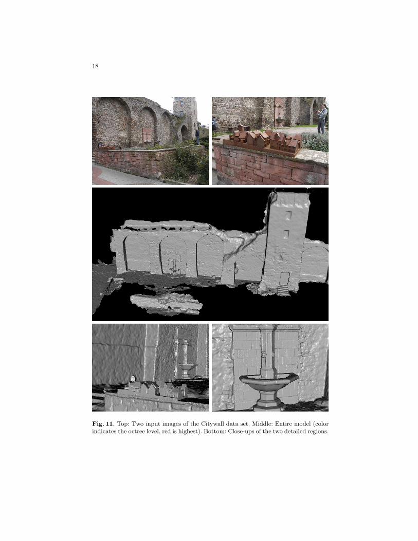
The Citywall data set consists of 487 images showing a large area around acity wall. The wall is sampled with medium resolution, two regions though aresampled with very high resolution: the fountain in the middle and a small sculp-ture of a city to the left (Figure 11 top). Our multi-resolution method is ableto reconstruct even fine details in the large scene where sample footprints differup to a factor of 209. In consequence, the reconstruction spans six octree levelsand detailed regions are triangulated about 32 times finer than low-resolutionregions. The middle image of Figure 11 shows the entire mesh whereas the bot-tom images show close-ups of the highly detailed surface regions. One can evenrecognize some windows of the small buildings in the reconstructed geometry.

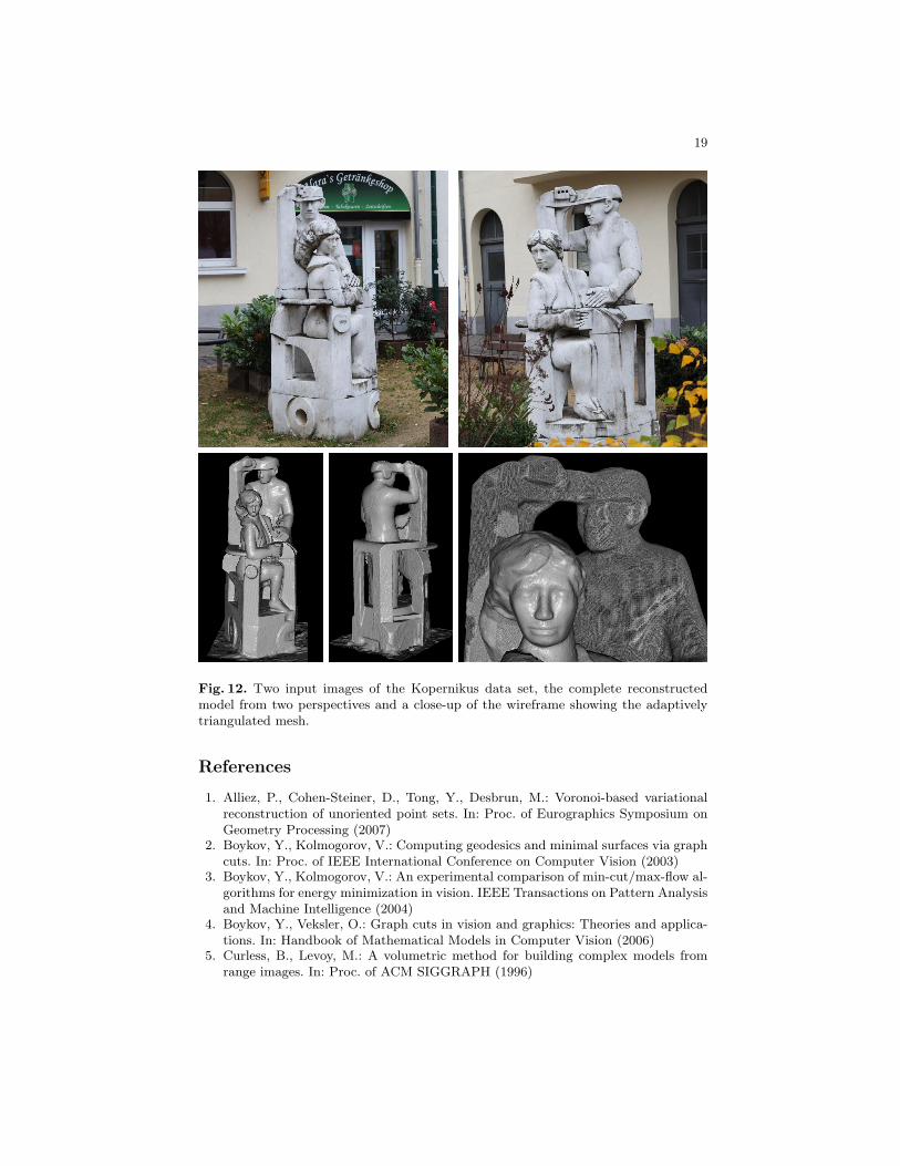
The Kopernikus data set (Figure 12) consists of 334 images showing a statuewith a man and a women. The underlying surface geometry is particularly chal-lenging due to its high genus. The data set is also multi-resolution in the sensethat we took close-up views of the area around the hands. We compare our recon-struction against VRIP [5] and the depth map fusion by Fuhrmann and Goesele[6] (Figure 13). It is clearly visible that our model contains significantly less noiseand shows no clutter around the real surface. Also, the complex topology of theobject is captured very well in comparison to the other methods. However, inregions with low-resolution geometry staircase artifacts are visible due to thesurface extraction from a binary signed distance field. This is also visible in thewireframe rendering in Figure 12 (bottom right) showing the dense triangulationof the women’s face versus the coarse triangulation of the men’s upper body.

9 Conclusion and future work

We presented a robust surface reconstruction algorithm that works on generalinput data. To our knowledge, except for the concurrent work of Fuhrmannand Goesele [6], we are the first to take the footprint of a sample point intoaccount during reconstruction. Together with a robust crust computation andan adaptive multi-resolution reconstruction approach we are able to reconstructfine detail in large-scale scenes. We presented results comparable to state-of-the-art techniques on a benchmark data set and proved our superiority on challenginglarge-scale outdoor data sets and objects with complex topology. The trianglemeshes are manifold and watertight and show an adaptive triangulation withsmaller triangles in regions where higher details were captured.

In future work, we plan to explore other ways to distribute a sample point’sconfidence over the volume, e.g., taking the direction to the sensor into account.This would allow us to better model the generally anisotropic error present inreconstructed depth maps.

Acknowledgements This work was supported in part by the DFG Emmy Noetherfellowship GO 1752/3-1.

18

Fig. 11. Top: Two input images of the Citywall data set. Middle: Entire model (colorindicates the octree level, red is highest). Bottom: Close-ups of the two detailed regions.

19

Fig. 12. Two input images of the Kopernikus data set, the complete reconstructedmodel from two perspectives and a close-up of the wireframe showing the adaptivelytriangulated mesh.

References

1. Alliez, P., Cohen-Steiner, D., Tong, Y., Desbrun, M.: Voronoi-based variationalreconstruction of unoriented point sets. In: Proc. of Eurographics Symposium onGeometry Processing (2007)

2. Boykov, Y., Kolmogorov, V.: Computing geodesics and minimal surfaces via graphcuts. In: Proc. of IEEE International Conference on Computer Vision (2003)

3. Boykov, Y., Kolmogorov, V.: An experimental comparison of min-cut/max-flow al-gorithms for energy minimization in vision. IEEE Transactions on Pattern Analysisand Machine Intelligence (2004)

4. Boykov, Y., Veksler, O.: Graph cuts in vision and graphics: Theories and applica-tions. In: Handbook of Mathematical Models in Computer Vision (2006)

5. Curless, B., Levoy, M.: A volumetric method for building complex models fromrange images. In: Proc. of ACM SIGGRAPH (1996)

20

Our results Depth map fusion VRIP

Fig. 13. Comparison of our reconstruction (left) with depth map fusion (middle) [6]and VRIP (right) [5].

6. Fuhrmann, S., Goesele, M.: Fusion of depth maps with multiple scales. In: Proc.of ACM SIGGRAPH Asia (2011)

7. Furukawa, Y., Curless, B., Seitz, S.M., Szeliski, R.: Towards internet-scale multi-view stereo. In: Proc. of IEEE Conference on Computer Vision and Pattern Recog-nition (2010)

8. Goesele, M., Snavely, N., Curless, B., Hoppe, H., Seitz, S.M.: Multi-view stereofor community photo collections. In: Proc. of IEEE International Conference onComputer Vision (2007)

9. Habbecke, M., Kobbelt, L.: A surface-growing approach to multi-view stereo recon-struction. In: Proc. of IEEE Conference on Computer Vision and Pattern Recog-nition (2007)

10. Hoppe, H., DeRose, T., Duchamp, T., McDonald, J., Stuetzle, W.: Surface recon-struction from unorganized points. In: Proc. of ACM SIGGRAPH (1992)

11. Hornung, A., Kobbelt, L.: Hierarchical volumetric multi-view stereo reconstructionof manifold surfaces based on dual graph embedding. In: Proc. of IEEE Conferenceon Computer Vision and Pattern Recognition (2006)

12. Hornung, A., Kobbelt, L.: Robust reconstruction of watertight 3D models fromnon-uniformly sampled point clouds without normal information. In: Proc. of Eu-rographics Symposium on Geometry Processing (2006)

13. Kazhdan, M., Bolitho, M., Hoppe, H.: Poisson surface reconstruction. In: Proc. ofEurographics Symposium on Geometry Processing (2006)

14. Labatut, P., Pons, J.P., Keriven, R.: Robust and efficient surface reconstructionfrom range data. Computer Graphics Forum (2009)

15. Lorensen, W.E., Cline, H.E.: Marching cubes: A high resolution 3D surface con-struction algorithm. In: Proc. of ACM SIGGRAPH (1987)

16. Manson, J., Schaefer, S.: Isosurfaces over simplicial partitions of multiresolutiongrids. In: Proc. of Eurographics (2010)

21

17. Middlebury multi-view stereo evaluation, http://vision.middlebury.edu/mview/18. Mucke, P., Klowsky, R., Goesele, M.: Surface reconstruction from multi-resolution

sample points. In: Proc. of Vision, Modeling and Visualization (2011)19. Project page, http://www.gris.tu-darmstadt.de/projects/multires-surface-recon/20. Seitz, S.M., Curless, B., Diebel, J., Scharstein, D., Szeliski, R.: A comparison and

evaluation of multi-view stereo reconstruction algorithms. In: Proc. of IEEE Con-ference on Computer Vision and Pattern Recognition (2006)

21. Shalom, S., Shamir, A., Zhang, H., Cohen-Or, D.: Cone carving for surface recon-struction. In: Proc. of ACM SIGGRAPH Asia (2010)

22. Sinha, S.N., Mordohai, P., Pollefeys, M.: Multi-view stereo via graph cuts on thedual of an adaptive tetrahedral mesh. In: Proc. of IEEE International Conferenceon Computer Vision (2007)

23. Snavely, N., Seitz, S.M., Szeliski, R.: Skeletal sets for efficient structure from mo-tion. In: Proc. of IEEE Conference on Computer Vision and Pattern Recognition(2008)

24. Vu, H.H., Keriven, R., Labatut, P., Pons, J.P.: Towards high-resolution large-scalemulti-view stereo. In: Proc. of IEEE Conference on Computer Vision and PatternRecognition (2009)

25. Zach, C., Pock, T., Bischof, H.: A globally optimal algorithm for robust TV-L1range image integration. In: Proc. of IEEE International Conference on ComputerVision (2007)