Hierarchical Modeling of IEEE 802.11 Multi-hopWireless Networks

Thiago AbreuUniversité Lyon 1 - LIP

Francethiago.wanderley@ens-lyon.fr

Bruno BaynatUniversité Pierre et Marie

Curie - LIP6France

bruno.baynat@lip6.fr

Thomas BeginUniversité Lyon 1 - LIP

Francethomas.begin@ens-lyon.fr

Isabelle Guérin-LassousUniversité Lyon 1 - LIP

Franceisabelle.guerin-lassous@ens-

lyon.fr

ABSTRACTIEEE 802.11 is implemented in many wireless networks, in-cluding multi-hop networks where communications betweennodes are conveyed along a chain. We present a modelingframework to evaluate the performance of flows conveyedthrough such a chain. Our framework is based on a hier-archical modeling composed of two levels. The lower levelis dedicated to the modeling of each node, while the upperlevel matches the actual topology of the chain. Our approachcan handle different topologies, takes into account Bit ErrorRate and can be applied to multi-hop flows with rates rang-ing from light to heavy workloads. We assess the ability ofour model to evaluate loss rate, throughput, and end-to-enddelay experienced by flows on a simple scenario, where thenumber of nodes is limited to three. Numerical results showthat our model accurately approximates the performance offlows with a relative error typically less than 10%.

Categories and Subject DescriptorsC.4 [Performance of Systems]: Modeling techniques

KeywordsMulti-hop wireless chains; Markov Chains; performance eval-uation; IEEE 802.11 modeling

1. INTRODUCTIONIEEE 802.11, based on CSMA/CA principles, is one of

the leading communication protocols for wireless networks.Its deployment has been largely supported by its distributedproperty as well as by the simplicity and the low cost asso-ciated with its implementation. Various underlying topolo-

Permission to make digital or hard copies of all or part of this work for personal orclassroom use is granted without fee provided that copies are not made or distributedfor profit or commercial advantage and that copies bear this notice and the full cita-tion on the first page. Copyrights for components of this work owned by others thanACM must be honored. Abstracting with credit is permitted. To copy otherwise, or re-publish, to post on servers or to redistribute to lists, requires prior specific permissionand/or a fee. Request permissions from permissions@acm.org.MSWiM’13, November 3–8, 2013, Barcelona, Spain.Copyright 2013 ACM 978-1-4503-2353-6/13/11 ...$15.00.http://dx.doi.org/10.1145/2507924.2507949.

gies for IEEE 802.11 exist. Clearly, the most frequent ex-ample is the infrastructure network, commonly referred toas a WiFi hotspot, where communications occur exclusivelybetween nodes and the access point. Other examples in-clude multi-hop wireless networks, where communicationsbetween nodes may involve relay nodes, that act like for-warding entities.

Throughout this paper we refer to the sequence of nodesinvolved in the communication between two nodes as beinga chain. The behavior and associate performance of sucha chain can not be easily derived since the latter is subjectto many factors, e.g. the number and position of nodes inthe chain, and it may exhibit complex phenomena like thefreezing period of backoff, the hidden node problem, etc.

Despite these intrinsic complexities, analytical models canrepresent a convenient means to forecast and explain theperformance of flows travelling along a multi-hop wirelessnetwork. However, only few models have been proposed forcharacterizing their behavior. Indeed, most of the analyticalstudies on IEEE 802.11 are devoted to either cell networks,or multi-hop networks with single-hop flow [2, 11, 5, 9]. Con-sidering the few works dealing with multi-hop flows [1, 6],they consider simplifying assumptions (e.g. buffers with infi-nite length to queue extra datagrams, ideal physical layer fortransmitting frames, specific scenarios where the network isoverloaded or even totally saturated) that significantly devi-ate from some of the fundamental properties arising in IEEE802.11 chains, and thus they may not be accurate when ap-plied to realistic scenarios.

We present new a modeling framework to evaluate theperformance of a flow conveyed through a chain. Our frame-work is based on a hierarchical modeling composed of twolevels. The lower level is dedicated to the modeling of eachnode, while the upper level takes into account the actualshape (topology) of the chain. Thus, given the shape of theactual chain, the channel degradation pattern due to BitError Rate and the rate of the flow conveyed through thechain, the model delivers approximate values for customaryperformance parameters, e.g. loss rate, throughput, end-to-end delay, using a simple fixed-point iteration between thetwo modeling levels.

The remainder of the paper is organized as follows. Sec-tion 2 reminds the principles of IEEE 802.11 protocol and

describes the considered scenario in this work. Section 3presents our modeling framework. In Section 4, we comparethe performance delivered by our model with the actual onescoming from a discrete-event simulator. Section 5 concludesthis paper.

2. SYSTEM DESCRIPTION

2.1 IEEE 802.11In this section, we remind the main principles of IEEE

802.11 DCF protocol [7]. Basically, the transmission of adatagram occurs as follows. First, the node continuouslysenses the channel until the latter is found to be idle fora time DIFS. Second, the node postpones the transmissionof the frame associated to this datagram by a time whoselength is randomly drawn within an interval determined bythe contention window (also denoted CW hereafter). Thislatter delay is expressed as a number of slot times and isreferred to as the backoff. Then, the backoff value is contin-ually decremented (by one) whenever the channel is sensedidle during an entire slot time. If the channel is sensed asbusy, the backoff value remains constant. It is said to bein freezing state. The backoff quits this freezing state, andhence resumes its decrement, if the channel is sensed idleduring a DIFS period. As the backoff value reaches zero, thenode can start its transmission. Note that a backoff periodcan be interrupted several times due to multiple transmis-sions in its neighborhood.

A node considers that its frame has been successfully trans-mitted to its neighbor node when it receives the acknowl-edgment. If the node does not receive an acknowledgmentbefore a timeout, which includes a SIFS, it assumes the cor-responding frame has been lost, and thus attempts to re-transmit it up to a given limit [7]. Note that at each retrans-mission of a frame, the contention window size is doubled. Ifthe transmission of a frame as well as the following retrans-missions fail, the node simply discards the correspondingdatagram. Finally, each successful transmission of a frame(as well as a complete discard) resets the contention windowto its initial value.

IEEE 802.11 includes an optional mechanism to avoid col-lisions, known as RTS/CTS. When activated, prior to eachframe transmission, a node sends a RTS (Request-to-Send)frame and should receive a CTS (Clear-to-Send) frame inthe aim of getting exclusive use of the channel. Note thatsince RTS/CTS has been shown to be inefficient in the caseof a chain [12], we did not consider it in our study.

2.2 Studied chain and associated scenarioWe consider the case of a wireless multi-hop chain with

N nodes (labeled from 1 to N). We now itemize the mainassumptions regarding our system. First, each node canonly communicate with its 1-hop neighbors. Second, thecarrier sense range of each node covers all its 2-hop neighbornodes. Third, we consider a non-perfect physical layer thataffects the channel quality, and can cause erroneous frametransmissions. We assume that the Bit Error Rate (BER)does only depend on the distance between nodes. Here, weuse the values reported in [8].

We assume that the network chain conveys a single flow,starting at one border node and traveling up to the otherborder node. The flow may represent the traffic generatedby a single (or multiple) user or application. A flow is com-

Workload 3 4

2

1

5

6

Transmission range of node 3Carrier sense range of node 3

Figure 1: A multi-hop chain with a single flow andN=6 nodes.

posed of equally sized datagrams. The rate at which thisflow generates datagrams determines the level of workloadof the chain. Note that our system will be described as beingin saturation if the flow always have datagrams to be sentacross the chain. Figure 1 illustrates a possible example ofour system with 6 nodes. As exhibited by this figure, nodesin the chain do not have to be aligned along a straight line,nor being equally spaced as long as they meet the assump-tions mentioned above.

We now detail the scenario that will be used as case studythroughout the next sections. In this scenario, we considera multi-hop chain with N=3 nodes that conveys a singleflow travelling from node 1 to node 3 through node 2. Weposition node 2 at different distances in between nodes 1and 3, and we consider several levels of rates for the flowworkload. Clearly, the performance of the flow will varyagainst the distance between the nodes since each distanceleads to a different BER, and thus to a different rate oferroneous frame transmission. Although this scenario doesnot face the hidden node problem (since all nodes are in thedetection range of each other), it has to cope with severalother issues, e.g. heavy dependence between nodes, freezingperiods of the backoff, recurrent starvation of the relay node.

3. HIERARCHICAL MODELINGWe have developed a hierarchical modeling framework

for performance evaluation of a general multi-hop wirelesschain. Our model is made of two levels: 1) a global high-level queueing network model and 2) several local low-levelMarkov chain models. In the global model, each queue isassociated with a node of the wireless chain, and the rout-ing between queues matches the topology of the chain. Inorder to parameterize the global model, we use several localMarkov chain models, each one being associated to a givenqueue of the global model, i.e., to a given node of the chain.As a first step in the development of this general framework,we describe our hierarchical model on a simple scenario inSections 3.1 and 3.2. As detailed in these two subsections,the inputs of the global model are the outputs of the localmodels, and vice versa. The performance of the resultingmodel will thus be the solution of a fixed-point iterative al-gorithm described in Section 3.3.

3.1 Global modelAs explained before, in this paper we restrict the descrip-

tion of the model to a simple scenario made of three nodes,

7 unsuccessful frame transmissions

buffer full

K1 K2

µ1 µ2workload

!"#

datagramlosses

!"#

successfultransmissions

λ1

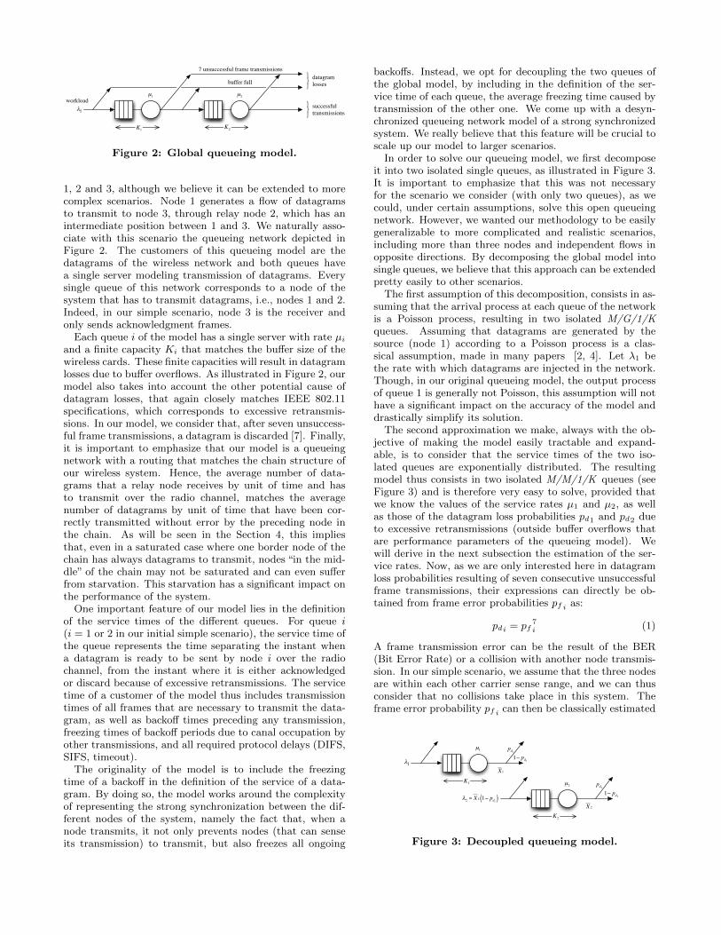
Figure 2: Global queueing model.

1, 2 and 3, although we believe it can be extended to morecomplex scenarios. Node 1 generates a flow of datagramsto transmit to node 3, through relay node 2, which has anintermediate position between 1 and 3. We naturally asso-ciate with this scenario the queueing network depicted inFigure 2. The customers of this queueing model are thedatagrams of the wireless network and both queues havea single server modeling transmission of datagrams. Everysingle queue of this network corresponds to a node of thesystem that has to transmit datagrams, i.e., nodes 1 and 2.Indeed, in our simple scenario, node 3 is the receiver andonly sends acknowledgment frames.

Each queue i of the model has a single server with rate µi

and a finite capacity Ki that matches the buffer size of thewireless cards. These finite capacities will result in datagramlosses due to buffer overflows. As illustrated in Figure 2, ourmodel also takes into account the other potential cause ofdatagram losses, that again closely matches IEEE 802.11specifications, which corresponds to excessive retransmis-sions. In our model, we consider that, after seven unsuccess-ful frame transmissions, a datagram is discarded [7]. Finally,it is important to emphasize that our model is a queueingnetwork with a routing that matches the chain structure ofour wireless system. Hence, the average number of data-grams that a relay node receives by unit of time and hasto transmit over the radio channel, matches the averagenumber of datagrams by unit of time that have been cor-rectly transmitted without error by the preceding node inthe chain. As will be seen in the Section 4, this impliesthat, even in a saturated case where one border node of thechain has always datagrams to transmit, nodes “in the mid-dle” of the chain may not be saturated and can even sufferfrom starvation. This starvation has a significant impact onthe performance of the system.

One important feature of our model lies in the definitionof the service times of the different queues. For queue i(i = 1 or 2 in our initial simple scenario), the service time ofthe queue represents the time separating the instant whena datagram is ready to be sent by node i over the radiochannel, from the instant where it is either acknowledgedor discard because of excessive retransmissions. The servicetime of a customer of the model thus includes transmissiontimes of all frames that are necessary to transmit the data-gram, as well as backoff times preceding any transmission,freezing times of backoff periods due to canal occupation byother transmissions, and all required protocol delays (DIFS,SIFS, timeout).

The originality of the model is to include the freezingtime of a backoff in the definition of the service of a data-gram. By doing so, the model works around the complexityof representing the strong synchronization between the dif-ferent nodes of the system, namely the fact that, when anode transmits, it not only prevents nodes (that can senseits transmission) to transmit, but also freezes all ongoing

backoffs. Instead, we opt for decoupling the two queues ofthe global model, by including in the definition of the ser-vice time of each queue, the average freezing time caused bytransmission of the other one. We come up with a desyn-chronized queueing network model of a strong synchronizedsystem. We really believe that this feature will be crucial toscale up our model to larger scenarios.

In order to solve our queueing model, we first decomposeit into two isolated single queues, as illustrated in Figure 3.It is important to emphasize that this was not necessaryfor the scenario we consider (with only two queues), as wecould, under certain assumptions, solve this open queueingnetwork. However, we wanted our methodology to be easilygeneralizable to more complicated and realistic scenarios,including more than three nodes and independent flows inopposite directions. By decomposing the global model intosingle queues, we believe that this approach can be extendedpretty easily to other scenarios.

The first assumption of this decomposition, consists in as-suming that the arrival process at each queue of the networkis a Poisson process, resulting in two isolated M/G/1/Kqueues. Assuming that datagrams are generated by thesource (node 1) according to a Poisson process is a clas-sical assumption, made in many papers [2, 4]. Let λ1 bethe rate with which datagrams are injected in the network.Though, in our original queueing model, the output processof queue 1 is generally not Poisson, this assumption will nothave a significant impact on the accuracy of the model anddrastically simplify its solution.

The second approximation we make, always with the ob-jective of making the model easily tractable and expand-able, is to consider that the service times of the two iso-lated queues are exponentially distributed. The resultingmodel thus consists in two isolated M/M/1/K queues (seeFigure 3) and is therefore very easy to solve, provided thatwe know the values of the service rates µ1 and µ2, as wellas those of the datagram loss probabilities pd1 and pd2 dueto excessive retransmissions (outside buffer overflows thatare performance parameters of the queueing model). Wewill derive in the next subsection the estimation of the ser-vice rates. Now, as we are only interested here in datagramloss probabilities resulting of seven consecutive unsuccessfulframe transmissions, their expressions can directly be ob-tained from frame error probabilities pf i as:

pdi = pf7i (1)

A frame transmission error can be the result of the BER(Bit Error Rate) or a collision with another node transmis-sion. In our simple scenario, we assume that the three nodesare within each other carrier sense range, and we can thusconsider that no collisions take place in this system. Theframe error probability pf i can then be classically estimated

K2

K1

µ1

µ2

λ2 = X1 1− pd1( )

X1

X 2

pd11− pd1

pd21− pd2

λ1

Figure 3: Decoupled queueing model.

from the BER that is function of the distance between thesender (say node i) and the receiver (node i+ 1), extractedfrom manufacturers card specifications [8].

All performance parameters of our global queueing modelcan then be obtained from the well known results of theM/M/1/K queue. The output throughput of station i, cor-responding to the average number of datagrams transmittedby unit of time from node i to node i+ 1, is:

Xi = µi(1− πi(0)) (2)

where πi(n) is the probability of having n customers in thei-th M/M/1/K isolated queue.

The average number of customers in queue i, correspond-ing to the average number of datagrams waiting or in trans-mission at node i, is given by:

Qi =

Ki∑n=1

nπi(n) (3)

From Little’s law, we can derive the mean sojourn time of anadmitted customer in queue i, corresponding to the averagetime a datagram that is not lost because of buffer overflow,stays in node i before being transmitted to node i + 1 (ordiscarded because of excessive retransmissions):

Ri =Qi

Xi

(4)

The utilization of queue i, corresponding to the proportionof time node i is not empty, is:

U i = 1− πi(0) (5)

And finally, from PASTA theorem, we can obtain the re-jection probability, corresponding to the probability that adatagram is rejected because the buffer of the destinationnode is full at its arrival instant:

pri = πi(Ki) (6)

3.2 Local modelsIn order to estimate the missing parameters of the global

queueing network model, i.e., the rates µi (i = 1, 2) of thetwo M/M/1/K queues, we propose to associate with eachqueue, a Continuous-Time Markov Chain (CTMC) describ-ing precisely the transmission process of a node accordingto the IEEE 802.11 DCF protocol.

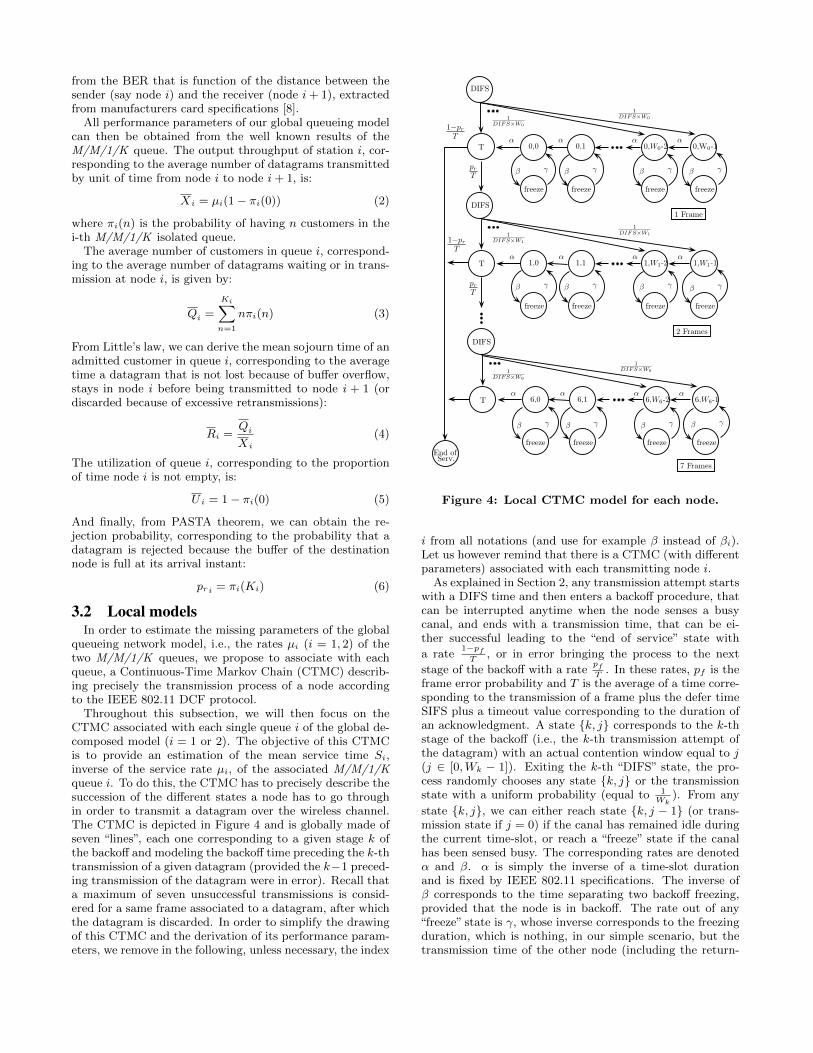
Throughout this subsection, we will then focus on theCTMC associated with each single queue i of the global de-composed model (i = 1 or 2). The objective of this CTMCis to provide an estimation of the mean service time Si,inverse of the service rate µi, of the associated M/M/1/Kqueue i. To do this, the CTMC has to precisely describe thesuccession of the different states a node has to go throughin order to transmit a datagram over the wireless channel.The CTMC is depicted in Figure 4 and is globally made ofseven “lines”, each one corresponding to a given stage k ofthe backoff and modeling the backoff time preceding the k-thtransmission of a given datagram (provided the k−1 preced-ing transmission of the datagram were in error). Recall thata maximum of seven unsuccessful transmissions is consid-ered for a same frame associated to a datagram, after whichthe datagram is discarded. In order to simplify the drawingof this CTMC and the derivation of its performance param-eters, we remove in the following, unless necessary, the index

freeze

0,W0-10,W0-20,10,0T

β γ

αααα

pr

T

1 Frame

DIFS

1DIFS×W0

1DIFS×W0

freeze freeze freeze

freeze

1,W1-11,W1-21,11,0T

β

αααα

pr

Tγ

2 Frames

DIFS

1DIFS×W1

1DIFS×W1

freeze freeze freeze

freeze

6,W6-16,W6-26,16,0T

β

αααα

γ

7 Frames

DIFS

1DIFS×W6

1DIFS×W6

freeze freeze freeze

β γβ γβ γ

β γβ γβ γ

β γβ γβ γ

End ofServ.

1−pr

T

1−pr

T

Figure 4: Local CTMC model for each node.

i from all notations (and use for example β instead of βi).Let us however remind that there is a CTMC (with differentparameters) associated with each transmitting node i.

As explained in Section 2, any transmission attempt startswith a DIFS time and then enters a backoff procedure, thatcan be interrupted anytime when the node senses a busycanal, and ends with a transmission time, that can be ei-ther successful leading to the “end of service” state with

a rate1−pf

T, or in error bringing the process to the next

stage of the backoff with a ratepfT

. In these rates, pf is theframe error probability and T is the average of a time corre-sponding to the transmission of a frame plus the defer timeSIFS plus a timeout value corresponding to the duration ofan acknowledgment. A state {k, j} corresponds to the k-thstage of the backoff (i.e., the k-th transmission attempt ofthe datagram) with an actual contention window equal to j(j ∈ [0,Wk − 1]). Exiting the k-th “DIFS” state, the pro-cess randomly chooses any state {k, j} or the transmissionstate with a uniform probability (equal to 1

Wk). From any

state {k, j}, we can either reach state {k, j − 1} (or trans-mission state if j = 0) if the canal has remained idle duringthe current time-slot, or reach a “freeze” state if the canalhas been sensed busy. The corresponding rates are denotedα and β. α is simply the inverse of a time-slot durationand is fixed by IEEE 802.11 specifications. The inverse ofβ corresponds to the time separating two backoff freezing,provided that the node is in backoff. The rate out of any“freeze” state is γ, whose inverse corresponds to the freezingduration, which is nothing, in our simple scenario, but thetransmission time of the other node (including the return-

T 12B 1

2B T 1

2B 1

2B T

T 13B 1

3B 1

3B T 1

3B 1

3B 1

3B T

1β

1β

1β

T 14B 1

4B 1

4B

1β

1β

14B T 1

4B 1

4B 1

4B 1

4B T

1 pauseframe

2 pausesframe

3 pausesframe

1β = B

2β = B

3β = B

time

time

time

1β

Figure 5: Illustration of the relation between β, npand B.

ing time of the acknowledgment) plus a DIFS time that isalways deferred before any backoff retake.

As a result, most of the parameters of this CTMC comedirectly from IEEE 802.11 specifications, except the frameerror probability pf and the rate β. As developped in Sec-tion 3.1, the frame error probability can be classically esti-mated from the BER and the distance between the considernode and the next one in the chain. Estimating the lastremaining parameter β is much more difficult and we nowturn our attention to it.

As explained before, it is easier to consider the inverse ofparameter β which corresponds to the mean time betweentwo successive backoff freezing (provided a node is in back-off). This quantity is related to the average number of freez-ing of the backoff of the considered node i, denoted as npand the mean backoff duration B. This is illustrated in Fig-ure 5, where the hashed areas correspond to freezing periodsof the backoff. If we assume that a) each backoff is pausedexactly one time, we can see from the figure that, in aver-age, 1/β = B; b) each backoff is paused exactly two times,2 × 1/β = B; and c) each backoff is paused exactly threetimes, 3 × 1/β = B. We can easily extend these results toan average number of pauses in the backoff, np, and obtainthe following (pretty intuitive) relation:

np

β= B (7)

It turns out that parameter β can be directly obtained fromthe estimation of the average number of backoff freezing andthe mean backoff duration. This last parameter can easilybe estimated from the following average:

B =CW1

2f1 + (CW1+CW2)

2f2 + · · ·+ (CW1+CW2+···+CW7)

2f7

f1 + 2f2 + · · ·+ 7f7(8)

where CWj is the size of the contention window at the j-thframe transmission attempt by assuming an initial CW of31 and a maximal CW of 1023, see Section 4):

CWj = min(24+j − 1, 1023) (9)

and fj is the probability that the transmission of a datagramrequires exactly j frames, and can be derived from the frameerror probability as:

fj = pj−1f (1− pf ) for j ≤ 6 and f7 = pf

6 (10)

Now it remains to estimate the average number of pauses inthe backoff of a node. Let us remind that the backoff of agiven node i is paused whenever any node j in the carriersense range of i makes a transmission. Now going back to

T1 B T1

time

B B

T2 T2

B T1B B

T2 T2

Figure 6: Relation between transmissions in neigh-bor nodes and backoff freezing in a saturated case.

our simplified scenario (with 3 nodes, but where only node 1and 2 transmit datagrams), let us consider backoff of node 1.Figure 6 illustrates the successive transmissions of node 1 ina saturated case, i.e., when node 1 has always datagramsto transmit. In this case, between two frame transmissionsthere is always a backoff that is paused by transmissionsof node 2. The average number of pauses of each backoffis thus equal to the average number of frame transmissionsof node 2 in between two conscutive frame transmissions ofnode 1. If we denote by F i the average number of framestransmitted by node i by unit of time (i = 1, 2), we thus

have: np1 = F2

F1. (Note that we need here to put back the

indexes corresponding to nodes in the notations.) We nowconsider the general case where node 1 is not saturated, il-lustrated in Figure 7. Between two transmissions there mayoccur an idle time (of average duration x on the figure) be-fore the beginning of the backoff. Some transmissions ofnode 2 freeze the backoff of node 1, whereas others do not(because they happen during idle periods of node 1). Theaverage number of pauses in the backoff of node 1 has thus

to be adjusted with a corrective factor δ1 as: np1 = F2

F1×δ1.

This corrective factor corresponds to the proportion of timenode 1 is idle between two successive frame transmissions:δ1 = y

x+y. The final question relies on estimating the frame

throughput F i, as well as the corrective factors δi. Intu-itively, the average number of frame transmissions by unitof time F i is related to node i datagram throughput Xi andthe corrective factor δi is related to node i utilization U i. Itturns out that both quantities are performance parametersthat can be derived from the global model described in theprevious subsection.

First, the frame throughput F i can easily be obtainedfrom the datagram throughput Xi of M/M/1/K queue i ofthe global model, by multiplying it by the average numberof frame transmissions necessary to transmit a datagram:

F i = Xi nf i (11)

where nf i is expressed from the fn probability as:

nf i =

7∑n=1

n fn (12)

T1 T1

time

B B

T2 T2

T1B B

T2 T2

x y z

S1

Figure 7: Relation between transmissions in neigh-bor nodes and backoff freezing in a non-saturatedcase.

Then in order to obtain the correcting factor δi, we first ex-press the utilization U i of queue i with notations of Figure 7:

U i =Si

Si + x(13)

and use it in the expression of the corrective factor:

δi =y

x+ y=

Si − zSi

1−Ui

Ui+ Si − z

(14)

where z is just the actual transmission time of a frame.Finally, by using together previous equations, we get the

following expression for the missing parameters βi:

βi =Xjnf j

Xinf i

δi

B(15)

with the convention that j = 2 if i = 1, and j = 1 if i = 2.Now that all the parameters of the CTMC have been es-

timated, we can use it to get a fair estimation of the servicerate µi of the associated M/M/1/K queue i. The inverse ofthis rate corresponds to the average time that is necessaryto reach the state “end of service”, starting from the first“DIFS” state of the Markov chain, and is given by:

1

µi= t0 + pf i × (t1 + pf i × (t2 + ...+ pf i × t6))))))) (16)

where tk corresponds to the average time spent by the pro-cess in “line” k of the CTMC:

tk = DIFS +Wk

2× r + T (17)

and r is the average time spent in any pair of loop states({k, j}, {freeze}):

r =1

α×(

1 +β

γ

)(18)

3.3 Fixed-point solution of the modelAs developed in the two previous subsections, the global

model takes as an input the service rates µi of all queues andprovides the global performance parameters, among whichdatagram throughputs Xi (relation (2)) and node utiliza-tions U i (relation (5)). Conversely, the local models assumeknown values of datagram throughputs Xi and node uti-lizations U i to parameterize the CTMCs (thanks to rela-tions (8)-(15)) and give estimations of the service rates µi

(relations (16)-(18)). It is then quite obvious to resort on afixed-point iteration to obtain the values of the subsequentparameters. We detail the iterative procedure below:

0. Initialize rates βi (with non-absurd values, e.g. by tak-ing npi = 1).

1. Calculate the service rates µi by solving the CTMCassociated with each node i of the chain (equation (16)-(18)).

2. Solve the global queueing model and derive its perfor-mance parameters (equations (2)-(6)).

3. Update rates βi (equations (8)-(15)).

4. Repeat algorithm until convergence.

Once the algorithm has converged, we can obtain the perfor-mance parameters of interests from the well parameterizedglobal model: the average throughput of datagrams that

DIFS 50µsSIFS 10µs

Time slot 20µsContention window size (min,max) 31, 1023

Frame transmission limit 7

Table 1: IEEE 802.11 parameters

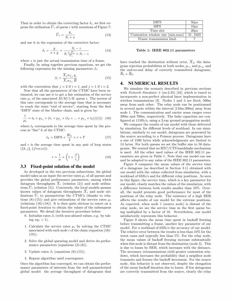
have reached the destination without error, X2, the data-gram rejection probabilities at both nodes, pr1 and pr2, andthe end-to-end delay of correctly transmitted datagrams,R1 +R2.

4. NUMERICAL RESULTSWe simulate the scenario described in previous sections

with Network Simulator 2 (ns-2.35) [10], which is tuned toincorporate a non-perfect physical layer implementation inwireless transmissions [3]. Nodes 1 and 3 are fixed, 500maway from each other. The relay node can be positionnedin several spots within the interval [110m,390m] away fromnode 1. The communication and carrier sense ranges cover399m and 700m, respectively. The links capacities are con-figured at 11Mb/s, using a 2-ray ground propagation model.

We compare the results of our model with those deliveredby simulation, for different levels of workload. In our simu-lations, similarly to our model, datagrams are generated bythe source according to a Poisson process. Datagrams havea size of 1500 bytes while acknowledgments are limited to14 bytes. For both queues we set the buffer size to 50 data-grams. We remind that no RTC/CTS handshake mechanismis used. All the other used values of the IEEE 802.11 pa-rameters are given in Table 1. Note that our model can useand be adapted to any value of the IEEE 802.11 parameters.

Figure 8 compares the mean values of the service timeof a datagram (as described in Section 3.1) obtained withour model with the values collected from simulation, with aworkload of 6Mb/s and for different relay positions. As seenin this figure, the service time, which is a key parameter forour model, closely matches the values of the simulation, witha difference between both results smaller than 10%. Over-all, the model presents good performance for most of thepositions of the relay node. The existence of a high BERaffects the results of our model for the extreme positions.As expected, when node 1 (source node) is distant of therelay node, we see the service time in the first queue be-ing multiplied by a factor of 10. Nevertheless, our modelsatisfactorily represents this behavior.

Figure 9 shows the mean time spent in backoff freezingbefore transmitting a frame, another key parameter of ourmodel. For a workload of 6Mb/s the accuracy of our model.The relative error between the results is less than 10% for theworst cases and typically less than 5%. For the relay node,the mean values of backoff freezing increase substantiallywhen this node is distant from the destination (node 3). Thisis due to losses by BER, which increases with the distance.The necessary retransmissions yield greater contention win-dows, which increases the probability that a neighbor nodetransmits and freezes the backoff decrement. For the sourcenode, this behavior is not observed, despite the elongationof the mean backoff duration due to losses. If few datagramsare correctly transmitted from the source, clearly the relay

100 150 200 250 300 350 4000

0.02

0.04

0.06

Distance source−relay (m)

Se

co

nd

s

Node 1 (simul.)

Node 1 (model)

Node 2 (simul.)

Node 2 (model)

Figure 8: Mean service times of datagrams for aworkload of 6Mb/s.

node will very likely go to starvation. Therefore, it will notbe able to freeze the backoff decrement at the source node.This behavior shows that there is no symmetry between thesource and relay nodes, which may not be obviously initially.

Figure 10 shows the performance of our model, regardingthe mean throughput of a node, datagram rejection proba-bility by buffer overflows and mean end-to-end delay. Theseperformance parameters correspond to characteristics of ourmodel, as seen in Equations (2), (6) and (4). Figure 10(a)shows the throughputs of both nodes obtained from ourmodel and from simulation, for a workload of 3Mb/s. Underthese circumstances, depending on the actual distance be-tween nodes 1 and 2, node 1 can be in saturation. We clearlysee that the relative error between the results of our modeland those from simulation is very low (around 3%). In awide range of relay positions (between 150m and 350m), wesee that the system is capable of conveying the entire work-load. On the other hand, when source and relay nodes areclose, the throughput of node 2 decreases due to high BERand the network can not cope with the workload. In theother extreme position (source and relay nodes are distant),due to BER, there are more retransmissions for node 1 withconsequent service time elongation and buffer overflows innode 1. Figure 10(d) shows that, when the system work-load is set to 6Mb/s, the best performance of the systemare obtained in several points around the middle positionfor node 2, where the effect of BER is less significant. Withthis workload, the system is not capable of conveying alldatagrams and is in saturation (buffer overflows).

Figure 10(b) and 10(e) compare the datagram rejectionprobabilities of our model with simulation, for the same lev-els of workload. The accuracy of our model is clearly seen,since the relative error, when comparing to the simulationresults, remains low for both cases (less than 5%). The re-jection probability for the relay node is significantly moreimportant when it is close to source node. This is due to

100 150 200 250 300 350 4000

0.002

0.004

0.006

0.008

0.01

Distance source−relay (m)

Se

co

nd

s

Node 1 (simul.)

Node 1 (model)

Node 2 (simul.)

Node 2 (model)

Figure 9: Mean backoff freezing duration for a work-load of 6Mb/s.

the high rate of arriving datagrams from node 1 and to theframe losses between nodes 2 and 3 due to high BER. Theselosses increase the frame retransmissions and the mean ser-vice time of a datagram for node 2, which leads to a higherbuffer occupation. Regarding the source node, it also losesseveral datagrams by buffer overflow whenever the BER isimportant. Moreover, for the workload of 6Mb/s, the chainis not capable of conveying the entire workload, and data-grams are rejected by the source node.

Finally, Figure 10(c) and 10(f) show the mean end-to-enddelay of a datagram. The relative errors between our modelresults and those from simulation are low, ranging from 3%(best cases) up to 10% (worst cases). As expected, thesevalues increase significantly when the BER is more impor-tant (long distances between nodes), leading to values up to12 times larger when compared to the best cases around themiddle position. To the best of our knowledge, our model isthe only one to also estimate this performance parameter.

Given the accuracy of our model, we believe it can be usedas a prediction tool to forecast the flow performance fordifferent positions of the relay node. Figure 11 shows thebehavior of the system throughput for several workloads,ranging from 0.1Mb/s up to 8Mb/s, and for five differentdistances between source and relay nodes. We can see theimpact of saturation in the overall throughput, when therelay node is 150m away from the source. This scenariopresents a performance degradation when the workload ex-ceeds a certain limit (around 3.2Mb/s). This behavior canbe exacerbated for other scenarios, and a prediction tool isthus of high importance, in order to to prevent the systemfrom such a performance degradation.

We have also developed and validated a model for the sce-nario where two independent flows are conveyed throughoutthe chain, each starting at one border node and traveling upto the other border node. However, due to space constraints,related results are not presented in this work.

5. CONCLUSIONIn this paper, we present a hierarchical modeling frame-

work to evaluate the performance of flows conveyed througha multi-hop wireless chain. This latter approach is thoughtto deal with different topologies of the chain, can handlevarious channel degradation patterns due to Bit Error Rateand can be applied to flows with rates ranging from lightto heavy workloads. The resulting model is simple to im-

2 4 6 81

1.5

2

2.5

3

3.5

workload (Mb/s)

Thro

ughput (M

b/s

)

150m

200m

250m

300m

350m

Figure 11: Evolution of the mean throughput as afunction of the workload.

100 150 200 250 300 350 4000

1

2

3

Distance source−relay (m)

Th

rou

gh

pu

t (M

b/s

)

Node 1 (simul.)

Node 1 (model)

Node 2 (simul.)

Node 2 (model)

(a) workload: 3Mb/s

100 150 200 250 300 350 4000

0.2

0.4

0.6

0.8

1

Distance source−relay (m)

Re

jectio

n P

rob

ab

ility

Node 1 (simul.)

Node 1 (model)

Node 2 (simul.)

Node 2 (model)

(b) workload: 3Mb/s

100 150 200 250 300 350 4000

0.2

0.4

0.6

0.8

Distance source−relay (m)

En

d−

to−

en

d d

ela

y (

s)

simul.

model

(c) workload: 3Mb/s

100 150 200 250 300 350 4000

2

4

6

8

Distance source−relay (m)

Th

rou

gh

pu

t (M

b/s

)

Node 1 (simul.)

Node 1 (model)

Node 2 (simul.)

Node 2 (model)

(d) workload: 6Mb/s

100 150 200 250 300 350 4000

0.2

0.4

0.6

0.8

1

Distance source−relay (m)R

eje

ctio

n P

rob

ab

ility

Node 1 (simul.)

Node 1 (model)

Node 2 (simul.)

Node 2 (model)

(e) workload: 6Mb/s

100 150 200 250 300 350 4000

0.5

1

1.5

2

Distance source−relay (m)

En

d−

to−

en

d d

ela

y (

s)

simul.

model

(f) workload: 6Mb/s

Figure 10: Mean throughput (a,d), rejection probability by buffer overflow (b,e) and end-to-end delay (c,f).

plement and to parameterize. Its solution is easily obtainedusing a simple fixed-point iteration.

We validate our modeling framework on a simple scenariowhere the number of nodes in the chain is limited to three,yet the positioning of the relay node and the rate of the in-coming flow may vary significantly. We compare the valuesprovided by our modeling approach for customary perfor-mance parameters, e.g. loss rate, throughput, end-to-enddelay, with simulation. Numerical results show that ourmodel is able to accurately approximate the performanceof flows. The relative difference is in general less than 10%.

AcknowledgmentsThis work was partially funded by the French National Re-search Agency (ANR) under the project ANR VERSO RES-CUE (ANR-10-VERS-003). The authors wish to thank NghiNguyen for his valuable help with ns-2.

6. REFERENCES[1] A. Aziz, M. Durvy, O. Dousse, and P. Thiran. Models

of 802.11 multi-hop networks: Theoretical insights andexperimental validation. In IEEE COMSNETS, 2011.

[2] G. Bianchi. Performance analysis of the IEEE 802.11distributed coordination function. In IEEE JSAC,18(3), 2000.

[3] M. Fiore.http://perso.citi.insa-lyon.fr/mfiore/research.html.

[4] M. Garetto, T. Salonidis, and E. W. Knightly.Modeling per-flow throughput and capturingstarvation in CSMA multi-hop wireless networks. InIEEE INFOCOM, 2006.

[5] M. Garetto, J. Shi, and E. W. Knightly. Modelingmedia access in embedded two-flow topologies ofmulti-hop wireless networks. In ACM MobiCom, 2005.

[6] M. M. Hira, F. A. Tobagi, and K. Medepalli.Throughput analysis of a path in an IEEE 802.11multihop wireless network. In IEEE WCNC, 2007.

[7] IEEE 802.11 Working Group and others. IEEE802.11-2012 Part 11: Wireless LAN Medium AccessControl (MAC) and Physical Layer (PHY)specifications. In IEEE 802.11 Wireless LANStandards, 2012.

[8] H. Intersil. Direct sequence spread spectrum basebandprocessor, February 2002.

[9] B. Nardelli and E. W. Knightly. Closed-formthroughput expressions for CSMA networks withcollisions and hidden terminals. In IEEE INFOCOM,2012.

[10] NS2. http://www.isi.edu/nsnam/ns/.

[11] I. Tinnirello, G. Bianchi, and Y. Xiao. Refinements onIEEE 802.11 distributed coordination functionmodeling approaches. In IEEE Transactions onVehicular Technology, 59(3), 2010.

[12] K. Xu, M. Gerla, and S. Bae. Effectiveness ofRTS/CTS handshake in IEEE 802.11 based ad hocnetworks. In Ad Hoc Networks, 1, 2003.