i

Hierarchical Flight Control System Synthesis

for Rotorcraft-based Unmanned Aerial Vehicles

by

Hyunchul Shim

B.A. (Seoul National University, Seoul, South Korea) 1991 M.S. (Seoul National University, Seoul, South Korea) 1993

A dissertation submitted in partial satisfaction of the

requirements for the degree of

Doctor of Philosophy in

Engineering-Mechanical Engineering

in the

GRADUATE DIVISION

of the

UNIVERSITY OF CALIFORNIA, BERKELEY

Committee in charge:

Professor S. Shankar Sastry, Chair Professor Andrew K. Packard

Professor J. Karl Hedrick Professor Edward A. Lee

Fall 2000

ii

The dissertation of Hyunchul Shim is approved:

Chair Date Date

Date

Date

University of California, Berkeley

Fall 2000

iii

Hierarchical Flight Control System Synthesis

for Rotorcraft-based Unmanned Aerial Vehicles

Copyright 2000

by

Hyunchul Shim

iv

Abstract

Hierarchical Flight Control System Synthesis

for Rotorcraft-based Unmanned Aerial Vehicles

by

Hyunchul Shim

Doctor of Philosophy in Mechanical Engineering

University of California, Berkeley

Professor S. Shankar Sastry, Chair

The Berkeley Unmanned Aerial Vehicle (UAV) research aims to design, implement, and analyze

a group of autonomous intelli gent UAVs and UGVs (Unmanned Ground Vehicles). The goal of this

dissertation is to provide a comprehensive procedural methodology to design, implement, and test

rotorcraft-based unmanned aerial vehicles (RUAVs). We choose the rotorcraft as the base platform

for our aerial agents because it offers ideal maneuverabili ty for our target scenarios such as the

pursuit-evasion game. Aided by many enabling technologies such as lightweight and powerful

computers, high-accuracy navigation sensors and communication devices, it is now possible to

construct RUAVs capable of precise navigation and intelli gent behavior by the decentralized onboard

control system. Building a fully functioning RUAV requires a deep understanding of aeronautics,

control theory and computer science as well as a tremendous effort for implementation. These two

aspects are often inseparable and therefore equally highlighted throughout this research.

The problem of multiple vehicle coordination is approached through the notion of a hierarchical

system. The idea behind the proposed architecture is to build a hierarchical multiple-layer system that

gradually decomposes the abstract mission objectives into the physical quantities of control input.

Each RUAV incorporated into this system performs the given tasks and reports the results through the

hierarchical communication channel back to the higher-level coordinator.

In our research, we provide a theoretical and practical approach to build a number of RUAVs

based on commercially available navigation sensors, computer systems, and radio-controlled

helicopters. For the controller design, the dynamic model of the helicopter is first built. The helicopter

exhibits a very complicated multi-input multi-output, nonlinear, time-varying and coupled dynamics,

which is exposed to severe exogenous disturbances. This poses considerable difficulties for the

identification, control and general operation. A high-fidelity helicopter model is established with the

lumped-parameter approach. With the lift and torque aerodynamic model of the main and tail rotors, a

v

nonlinear simulation model is first constructed. The control models of the RUAVs used in our

research are derived by the application of a time-domain parametric identification method to the flight

data of target RUAVs. Two distinct control theories, namely classical control theory and modern

linear robust control theory, are applied to the identified model. The proposed controllers are

validated in a nonlinear simulation environment and tested in a series of test flights.

With the successful implementation of the low-level vehicle controller, the guidance layer is

designed. The waypoint navigator, which decides the adequate flight mode and the associated

reference trajectory, serves as an intermediary between the low-level vehicle control layer and the

high-level mission-planning layer. In order to interpret the abstract mission planning to commands

that are compatible with the low-level structure, a novel framework called Vehicle Control Language

(VCL) is developed. The key idea of VCL is to provide a mission-independent methodology to

describe given flight patterns. The VCL processor and vehicle control layer are integrated into the

hierarchical control structure, which is the backbone of our intelli gent UAV system. The proposed

idea is validated in the simulation environment and then fully tested in a series of flight tests.

_______________________

S. Shankar Sastry

Chair

vi

Contents

List of Figures................................................................................................. ix

List of Tables................................................................................................. xii

List of Symbols.............................................................................................xiii

1. Introduction ................................................................................................. 1

1.1 Overview of UAV Research.............................................................................................2

1.2 Hierarchical Vehicle Management Structure.....................................................................6

1.3 Relevant Research............................................................................................................6

1.4 Project History..................................................................................................................9

1.5 Contributions..................................................................................................................13

1.6 Scope of This Dissertation................................................................................................1

2. Helicopter Dynamics Modeling and System Identification.....................18

2.1 Coordinate Systems and Transformations.......................................................................19

2.1.1 Inertial Reference System and ECEF System..............................................................19

2.1.2 Tangent Plane Coordinate System...............................................................................21

2.1.3 Body Coordinate System............................................................................................22

2.1.3.1 Euler Angles............................................................................................23

2.1.3.2 Quaternion Representation.......................................................................24

2.1.3.3 Direction Cosine......................................................................................25

2.2 General Helicopter Model...............................................................................................27

2.2.1 Kinematic-Dynamic Equation of the Helicopter..........................................................28

2.2.2 Main Rotor.................................................................................................................31

2.2.3 Tail Rotor...................................................................................................................43

2.2.4 Stabilizer Fins............................................................................................................44

2.2.5 Fuselage.....................................................................................................................45

vii

2.2.6 External Factors.........................................................................................................46

2.2.7 Helicopter Hover Model.............................................................................................46

2.2.8 Experimental Hover Model.........................................................................................57

3. Hardware, Software, and Vehicle Integration.........................................66

3.1 Vehicle Platform.............................................................................................................67

3.1.1 Ursa Minor Series-Kyosho Concept 60.......................................................................67

3.1.2 Ursa Major Series-Bergen Industrial Twin.................................................................73

3.1.3 Ursa Magna Series-Yamaha R-50...............................................................................74

3.1.4 Ursa Maxima Series-Yamaha RMAX.........................................................................77

3.2 Navigation and Control System.......................................................................................82

3.2.1 Flight Computer System.............................................................................................83

3.2.2 Navigation Sensors.....................................................................................................87

3.2.2.1 Inertial Navigation System.......................................................................88

3.2.2.2 Global Positioning System.......................................................................91

3.2.2.3 INS/GPS Combination .............................................................................93

3.2.2.4 Ultrasonic Sensors....................................................................................95

3.2.3 Servomotor Control.................................................................................................... 97

3.3 Wireless Communication................................................................................................97

3.4 Ground Station...............................................................................................................99

3.5 Software Architecture................................................................................................... 100

4. Hierarchical Flight Control System Synthesis.......................................109

4.1 Regulation Layer..........................................................................................................111

4.1.1 Classical Controller Design......................................................................................113

4.1.2 - Synthesis Controller Design.................................................................................126

4.2 Waypoint Navigation.................................................................................................... 138

4.2.1 Vehicle Control Language........................................................................................144

4.2.2 Operation of VCL-based Waypoint Navigator..........................................................146

4.2.3 Validation of Waypoint Navigator............................................................................151

5. Conclusion...............................................................................................164

Appendix A Hardware Configuration of Berkeley RUAVs...................167

viii

A.1 Ursa Minor 3................................................................................................................167

A.2 Ursa Magna2................................................................................................................168

A.3 Ursa Maxima2..............................................................................................................171

A.4 Servomotor Control......................................................................................................173

Appendix B Data Structure......................................................................179

Appendix C Helicopter Operation...........................................................183

Appendix D Glossary................................................................................186

Bibliography ................................................................................................187

ix

List of Figures

Figure 1.1 First Navy RUAV: Gyrodyne QH-50 “DASH” .................................................................3

Figure 1.2 Tilt-rotor UAV: The Bell Eagle Eye..................................................................................4

Figure 1.3 Hierarchical flight control system.....................................................................................7

Figure 2.1 Geodetic reference coordinate system.............................................................................21

Figure 2.2 Tangent plane coordinate system....................................................................................21

Figure 2.3 Helicopters with different configuration..........................................................................27

Figure 2.4 Free body diagram of helicopter with respect to body coordinate system.........................30

Figure 2.5 Blade element method.................................................................................................... 32

Figure 2.6 Thrust vs (a) 0mθ , (b) cV .................................................................................................37

Figure 2.7 Swashplate and pitch level configuration........................................................................39

Figure 2.8 Rotor swashplate and flapping angles relationship...........................................................40

Figure 2.9 Bell-Hiller Stabilizer system...........................................................................................42

Figure 2.10 Stabilizer fins of R-50 (left) and Concept 60 (right).......................................................45

Figure 2.11 Block diagram representation of helicopter dynamics....................................................50

Figure 2.12 Sample flight data for system identification of Ursa Magna 2........................................61

Figure 2.13 The procedure of system identification using PEM........................................................62

Figure 2.14 The original response and estimated response by the identified model...........................64

Figure 3.1 Ursa Minor 1 in the payload test (April 1997).................................................................69

Figure 3.2 Ursa Minor 1 configured as a trainer...............................................................................70

Figure 3.3 Ursa Minor 2 in different configurations.........................................................................71

Figure 3.4 Ursa Minor 3 based on Kyosho Concept 60SR II Graphite.............................................72

Figure 3.5 Bergen Industrial Twin helicopter with shock absorbing landing gear.............................73

Figure 3.6 The servomotor configuration for swashplate actuation of Yamaha R-50........................74

Figure 3.7 Ursa Magna 2 based on Yamaha R-50 industrial helicopter............................................76

Figure 3.8 Block diagram of control signal flow in Yamaha R-50....................................................77

Figure 3.9 YACS system for Yamaha RMAX..................................................................................78

Figure 3.10 Detailed views of Yamaha RMAX................................................................................79

x

Figure 3.11 Ursa Maxima 2 based on Yamaha RMAX industrial helicopter.................................... 80

Figure 3.12 Fully equipped RUAV fleet at UC Berkeley..................................................................82

Figure 3.13. PC 104 stack (flight computer for Ursa Minor 3)..........................................................83

Figure 3.14 Interconnection diagram of onboard flight computer based on PCI local bus.................86

Figure 3.15 Inertial instruments: Boeing DQI-NP (left) Systron-Donner MotionPak™ (right)..........90

Figure 3.16 Boeing INS DQI-NP installed on Ursa Minor3(left) and Ursa Magna2 (right)..............90

Figure 3.17 NovAtel GPS Card (left) and L1/L2 antenna installed on R-50 (right)...........................93

Figure 3.18 Desirable INS/GPS installation on Ursa Minor 3...........................................................95

Figure 3.19 The measurement from two ultrasonic sensors of Ursa Magna 2.................................... 96

Figure 3.20 Communication architecture of Berkeley UAV/UGV/SMS Testbed..............................99

Figure 3.21 Ground monitoring station enhanced with GUI...........................................................100

Figure 3.22 System architecture of QNX RTOS.............................................................................104

Figure 3.23. Block diagram of VMS..............................................................................................104

Figure 3.24 Flowchart of process DQIGPS....................................................................................105

Figure 3.25 Flowchart of DQICONT.............................................................................................106

Figure 3.26 Flowchart for VCOMM..............................................................................................107

Figure 3.27 Flowchart for ULREAD..............................................................................................107

Figure 3.28 Real-time performance of onboard flight control software...........................................108

Figure 4.1 Modified hierarchical vehicle control system................................................................110

Figure 4.2 SISO representation of helicopter dynamics.................................................................. 114

Figure 4.3 Attitude Compensator Design.......................................................................................116

Figure 4.4 Velocity compensator design........................................................................................117

Figure 4.5 Position compensator design.........................................................................................118

Figure 4.6 Heave dynamics compensator design............................................................................119

Figure 4.7 Yaw dynamics compensator design...............................................................................119

Figure 4.8 The architecture of proposed SISO multi-loop controllers.............................................121

Figure 4.9 Ursa Magna 2 in automatic hover..................................................................................121

Figure 4.10 Experiment result of autonomous hovering of Ursa Magna 2.......................................122

Figure 4.11 Experiment results of autonomous hovering on Ursa Minor 3......................................123

Figure 4.12 Ursa Minor 3 in autonomous hover above the ship deck simulator...............................125

Figure 4.13 LFT representation of -synthesis framework..............................................................126

Figure 4.14 Singular value plot of the attitude dynamics of Ursa Magna........................................128

Figure 4.15 Interconnection diagram for -synthesis controller design...........................................128

Figure 4.16 Unstructured input uncertainty model..........................................................................129

xi

Figure 4.17 The Noise weighting functions....................................................................................131

Figure 4.18 The step response of the reference model.................................................................... 132

Figure 4.19 Performance weighting...............................................................................................133

Figure 4.20 The actuator weighting...............................................................................................133

Figure 4.21 µ bounds during the D-K iteration...............................................................................135

Figure 4.22 The singular value plot of the µ-attitude controller......................................................136

Figure 4.23 Experiment results of attitude regulation by -synthesis controller..............................137

Figure 4.24 State transition diagram of helicopter control..............................................................139

Figure 4.25 Hierarchical architecture of VCL processing...............................................................147

Figure 4.26 Reference yaw angle profile........................................................................................148

Figure 4.27 The acceleration, velocity, and position profile for low-speed forward flight...............150

Figure 4.28 Flowchart of VCL-based waypoint navigation in batch mode......................................151

Figure 4.29 The validation method using MATLAB/Simulink ......................................................152

Figure 4.30 Simulink model for waypoint navigation.....................................................................153

Figure 4.31 Sample VCL code for FlyTo maneuvers................................................................... 154

Figure 4.32 Simulation results of FlyTo maneuvers.................................................................... 155

Figure 4.33 Experiment result of FlyTo maneuvers.................................................................... 156

Figure 4.34 Sample VCL code for MoveTo maneuvers.................................................................159

Figure 4.35 Simulation results of MoveTo commands................................................................... 160

Figure 4.36 Experiment result of MoveTo commands in Figure 4.34.............................................161

Figure A.1 Flight computer layout of Ursa Minor 3.......................................................................167

Figure A.2 Flight computer layout of Ursa Magna 2......................................................................169

Figure A.3 Inside view of Ursa Magna 2 FCS................................................................................170

Figure A.4 The information flow in the avionics of Ursa Maxima 2...............................................171

Figure A.5 Avionics for Ursa Maxima 2........................................................................................172

Figure A.6 The characteristics of PWM signal for servomotors......................................................173

Figure A.7 Schematic diagram of one channel in TOB................................................................... 175

Figure A.8 Take-over board for Ursa Magna 2 FCS.......................................................................175

Figure A.9 Signal flow in Ursa Minor 3.........................................................................................176

Figure A.10 The signal flow in Ursa Magna 2................................................................................176

Figure A.11. PWM signal diagram for Yamaha R-50.....................................................................177

Figure A.12 Schematic diagram of Take-over Board......................................................................178

Figure C.1 Aerial view of the test flight site in Richmond, California.............................................184

Figure C.2 The operation of the ground station for Berkeley UAV research................................... 185

xii

List of Tables

Table 2-1 Parameters for Ursa Minor 2 for simulation model...........................................................56

Table 2-2 Eigenvalues of the identified helicopter system................................................................63

Table 3-1 Specifications of Berkeley RUAV platform.....................................................................81

Table 3-2 Specification of FCS........................................................................................................85

Table A-1 Interrupt and base address setting of Ursa Minor 3 FCS................................................168

Table A-2 Interrupt and base address setting of Ursa Magna 2 FCS...............................................169

xiii

List of Symbols

a : semimajor axis length of the elli psoidal approximation of the Earth

0a : coning angle of main rotor

1A : lateral cyclic pitch

1sa : longitudinal flapping angle of main rotor

b : semiminor axis length of the elli psoidal approximation of the Earth

b : number of blades in a rotor system

1B : longitudinal cyclic pitch

1sb : lateral flapping angle of main rotor

dc : drag coefficient of a blade

D : drag force of rotor

1s

dMda : Flapping stiffness in pitch direction

1s

dRdb : Flapping stiffness in roll direction

e : eccentricity of the elli psoidal approximation of the Earth

f : flatness of the elli psoidal approximation of the Earth

g : gravitational acceleration

h : vertical distance between the C.G. location and the acting point of a force

, ,x y zp p pK K K : Feedback gain for , ,x y zp p p channel, respectively

, ,u v wK K K : Feedback gain for u, v, w channel, respectively

, ,K K KΦ Θ Ψ : Feedback gain for roll, pitch, and yaw channel, respectively

l : longitudinal distance between the C.G. location and the acting point of a force

m : mass of helicopter

1,2,3,4,5,6m : temporary variables for closed-form thrust equation

bm : unit mass of blade

1, ,10n"

: temporary variables for closed-form torque equation

xiv

p : roll rate

Q : anti-torque of rotor

q : quaternion

q : pitch rate

1,2,3,4q : components of a quaternion

,M TQ : Torque of main and tail rotor, respectively

R : radius of a rotor (often referring to the main rotor diameter)

r : yaw rate

0R : inner radius of a rotor where the effective blade section starts

A B→R : rotational matrix from coordinate frame A to coordinate frame B

T : thrust of a rotor

,M TT : Thrust of main and tail rotor, respectively

1sau : input to the longitudinal flapping

1sbu : input to the lateral flapping

refru : reference input to the yaw rate feedback system

Muθ : input to the main rotor collective pitch

Tuθ : input to the tail rotor collective pitch

V : velocity vector

CV : vertical climb velocity of a helicopter

AW : Actuator weighting function

NW : Noise weighting function

PW : Performance weighting function

QW : Handling quality weighting function

UW : Uncertainty weighting function

X : position vector

y : lateral distance between the C.G. location and the acting point of a force

( , , )I I Ixx yy zz : mass moment of inertia in x,y,z-direction of body coordinate system

( , , )x y zp p p : position vector in local Cartesian coordinate

( ), ,i i iR M N : moment in x, y, and z-direction exerting on i-component, respectively

xv

( ), ,u v w : body velocity in x, y, and z-direction

( ), ,i i iX Y Z : body force in x, y, and z-direction exerting on i-component, respectively

Φ : roll angle of Euler angle representation

φ : longitude in geodetic coordinate system

λ : latitude in geodetic coordinate system

µ : structured singular value

Θ : pitch angle of Euler angle representation

θ : pitch angle of rotor

ρ : density of air

σ : singular value of a matrix

fτ : time constant of rotor flapping in the Bell-Hill er stabili zer system

Ψ : yaw angle of Euler angle representation; or azimuth angle of main rotor rotation

Ω : angular velocity of main and tail rotors

ΩΩ : angular velocity tensor

ωω : angular velocity vector

Superscripts TP : tangent-plane b : body frame

Subscripts

M, T, H, V, F : main rotor, tail rotor, horizontal stabili zer, vertical stabili zer, and fuselage,

respectively.

xvi

Acknowledgements I believe that I am truly privileged to participate in this fascinating project as a founding

member since 1996. I would like to give my deepest gratitude to Professor Shankar Sastry for his

guidance, insight, and vision on this project. I would like to thank Professor Andy K. Packard, who

has guided and encouraged my work with such passion and sincerity for knowledge, teaching and

care. Also I would like to thank Professor J. Karl Hedrick and Professor Edward A. Lee for their time

and valuable advices on my dissertation.

I would like to thank my research fellows Hoam Chung, Frank Hoffman, Jin Kim, John Koo,

Cedric Ma, Omid Shakernia, Cory Sharp, Rene Vidal for their help, advice, and cooperation for many

years.

I would like to thank Peter Ray in Electronics Research Laboratory of EECS department of UC

Berkeley, whose trust and encouragement brought my research and our group this far. I am also very

grateful to Judy Liebman, who proofread my dissertation in great detail.

I am pleased to acknowledge the financial support of the Army Research Office DAAH04-96-

1-0341 and by the Office of Naval Research under Grants N00014-97-1-0946, and DARPA F33615-

98-C-3614.

I would like to thank my previous advisor Professor Masayoshi Tomizuka in ME department

for allowing my study in Berkeley. My experience in motion control in his laboratory is also a

valuable part of my stay in Berkeley.

I would like to thank my research advisor back in my Master’s degree, Professor Kyo-Il Lee in

Seoul National University, Korea, for starting the pioneering research of helicopter control back in

1991. My experience in his lab certainly set the direction of my research. Also I would like to thank

Eun-Ho Lee for his insight on the future of autonomous helicopter research.

My special thanks go to my family. I would like to thank my parents, who taught me to take

chances for better things in my life. Also my gratitude to my late grandmother, who has offered me

unconditional love and care. I thank my brothers for their care and wish the best in their career.

In retrospect, this project did start humble but have grown to be a great success as now. There

are many happy times and many disappointing moments, but now I am very happy because all the

hardship I had to go through mostly alone finally paid off.

Above all, all the glory to God for everything that He has provided in my life, especially during

my years in Berkeley. “He who began a good work in you will complete it until the day of Jesus

Christ.”

1

Chapter 1

1.Introduction

The Berkeley UAV (Unmanned Aerial Vehicle) research aims to synthesize, implement, and

analyze a hybrid system consisting of multiple agents. These agents actively operate, interact,

cooperate, and achieve the given abstract tasks using the provided autonomy and intelli gence in

poorly known or completely unknown environment. This goal encompasses diverse fields of science

and technology such as control theory, hybrid system theory, artificial intelli gence, probabili stic

reasoning, and vision-based servoing to name a few. Although the project was originally initiated for

the creation of single UAV, it has diversified into many subgroups. Since the beginning of our project

in 1996, remarkable research efforts have been made in many fields such as hybrid system theory and

analysis [1], multiple agent coordination [2,3], map building, colli sion avoidance, and vehicle

stabili zation and control [4,5,6].

Among these many topics, the research on UAV flight system design remains the original and

fundamental one because it is the cornerstone technology that provides the testbed upon which other

abstract-level research can be implemented and evaluated. The UAV system design problem alone

encompasses many challenging research topics such as system identification, feedback control

system, navigation sensor design and implementation, hybrid systems, signal processing, realtime

control software design, and component-level mechanical-electronic integration. Indeed, UAV

development is a showcase of diverse fields of science and technology.

The Berkeley UAV team strives to construct a fleet of UAV systems that are endowed with

intelli gence and autonomy to independently accomplish the given abstract commands while

interacting with other agents in the neighborhood. The UAV is built by putting together state-of-the-

art navigation sensors and high-performance onboard computer systems with realtime software

control and background optimization processes, on a commercially available radio-controlled small-

2

size helicopter. The sensing capabili ty of the vehicle is extended by additional sensor systems such as

vision processor, laser range finder and so forth. The vehicle communicates with other agents and the

ground posts through the broadband wireless communication device, which will be capable of

dynamic network IP forwarding. The vehicle will be truly autonomous when it is capable of self-start

and automatic recovery with a single click of a button on the screen of the vehicle-monitoring

computer. The individual UAVs are integrated with the overall system through the hierarchical

system structure so that they can perform the given task in a cooperative manner. A high-level

mission command is decomposed into a set of low-level vehicle stabili zation and control commands

associated with the proper flight mode and reference trajectory. In the following, we briefly overview

the relevant technologies of the UAV system and the hierarchical architecture.

1.1 Overview of UAV Research

A UAV indicates an airframe that is capable of performing given missions autonomously

through the use of onboard sensors and manipulation systems. Any type of aircraft may serve as the

base airframe for a UAV application. Traditionally, the fixed-wing aircraft have been favored as the

platform because of many good reasons: they are simple in structure, efficient, and easy to build and

maintain. The autopilot design is easier for fixed-wing aircrafts than for rotary-wing aircrafts because

the fixed-wing aircrafts have relatively simple, symmetric, and decoupled dynamics. Some fixed-

wing UAVs (FUAVs), Pioneer UAV from Israel for example, have very successful records in actual

field operations. However, rotorcraft-based UAVs have been desirable for certain applications where

the unique flight capabili ty of the rotorcraft is required. The rotorcraft can take off and land within

limited space. They can also hover, and cruise at very low speed. Research of Rotorcraft-based UAVs

has finally become an active area during the last decade although one of the first RUAVs, Gyrodyne

QH-50, made its debut in 1958. One of the driving forces of the overdue proliferation of RUAVs may

be attributed to the maturing technologies that became available during the last 10 years, such as

rotorcraft dynamics, control system theory and application, high-accuracy small navigation systems

and GPS.

While building a fixed-wing aircraft that meets the given requirements such as payload is

relatively easy, building a custom-designed helicopter requires tremendous knowledge, time, and

effort. The market for the helicopter platform for RUAV development is very small and specialized.

Most of the above reasons contribute to the general understanding that RUAVs are more expensive

and more difficult to operate than FUAVs. However, only RUAVs can perform some applications

3

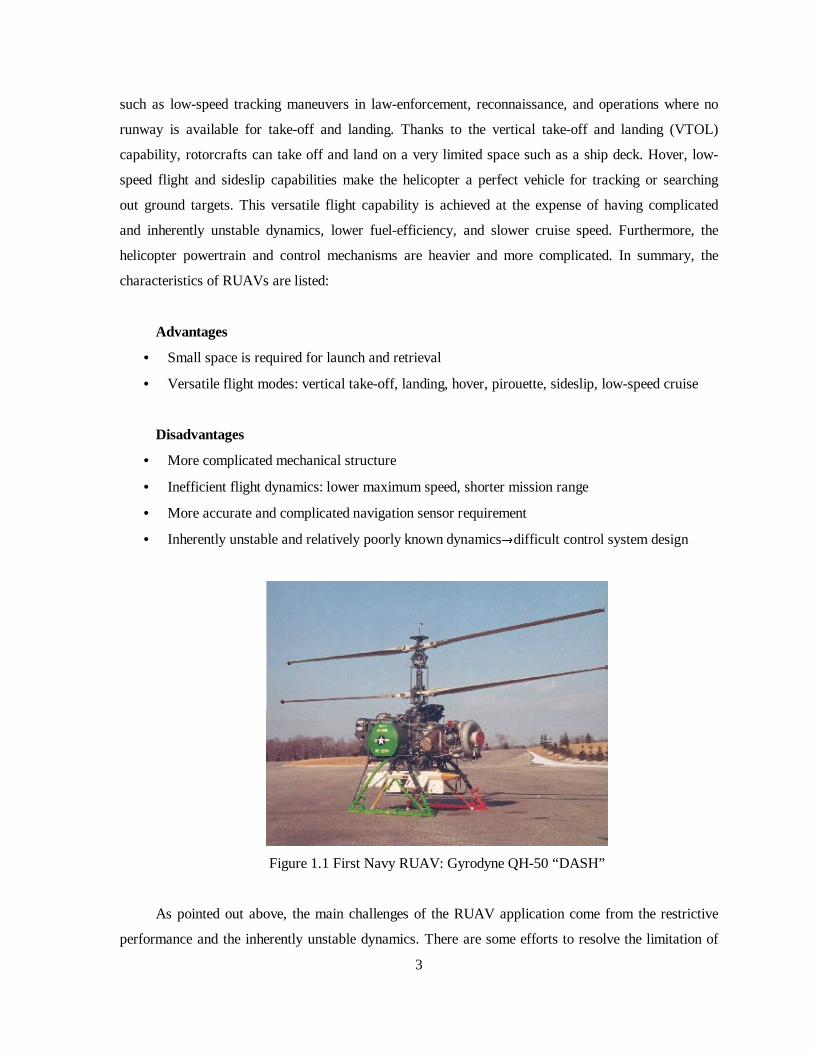
such as low-speed tracking maneuvers in law-enforcement, reconnaissance, and operations where no

runway is available for take-off and landing. Thanks to the vertical take-off and landing (VTOL)

capabili ty, rotorcrafts can take off and land on a very limited space such as a ship deck. Hover, low-

speed flight and sideslip capabili ties make the helicopter a perfect vehicle for tracking or searching

out ground targets. This versatile flight capabili ty is achieved at the expense of having complicated

and inherently unstable dynamics, lower fuel-efficiency, and slower cruise speed. Furthermore, the

helicopter powertrain and control mechanisms are heavier and more complicated. In summary, the

characteristics of RUAVs are listed:

Advantages

• Small space is required for launch and retrieval

• Versatile flight modes: vertical take-off, landing, hover, pirouette, sideslip, low-speed cruise

Disadvantages

• More complicated mechanical structure

• Inefficient flight dynamics: lower maximum speed, shorter mission range

• More accurate and complicated navigation sensor requirement

• Inherently unstable and relatively poorly known dynamicsdifficult control system design

Figure 1.1 First Navy RUAV: Gyrodyne QH-50 “DASH”

As pointed out above, the main challenges of the RUAV application come from the restrictive

performance and the inherently unstable dynamics. There are some efforts to resolve the limitation of

4

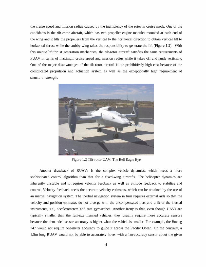
the cruise speed and mission radius caused by the inefficiency of the rotor in cruise mode. One of the

candidates is the tilt-rotor aircraft, which has two propeller engine modules mounted at each end of

the wing and it tilts the propellers from the vertical to the horizontal direction to obtain vertical li ft to

horizontal thrust while the stubby wing takes the responsibili ty to generate the lift (Figure 1.2). With

this unique lift/thrust generation mechanism, the tilt-rotor aircraft satisfies the same requirements of

FUAV in terms of maximum cruise speed and mission radius while it takes off and lands vertically.

One of the major disadvantages of the tilt-rotor aircraft is the prohibitively high cost because of the

complicated propulsion and actuation system as well as the exceptionally high requirement of

structural strength.

Figure 1.2 Tilt-rotor UAV: The Bell Eagle Eye

Another drawback of RUAVs is the complex vehicle dynamics, which needs a more

sophisticated control algorithm than that for a fixed-wing aircrafts. The helicopter dynamics are

inherently unstable and it requires velocity feedback as well as attitude feedback to stabili ze and

control. Velocity feedback needs the accurate velocity estimates, which can be obtained by the use of

an inertial navigation system. The inertial navigation system in turn requires external aids so that the

velocity and position estimates do not diverge with the uncompensated bias and drift of the inertial

instruments, i.e., accelerometers and rate gyroscopes. Another irony is that, even though UAVs are

typically smaller than the full-size manned vehicles, they usually require more accurate sensors

because the demanded sensor accuracy is higher when the vehicle is smaller. For example, the Boeing

747 would not require one-meter accuracy to guide it across the Pacific Ocean. On the contrary, a

1.5m long RUAV would not be able to accurately hover with a 1m-accuracy sensor about the given

5

waypoint. This observation alone asserts the complication of the onboard navigation and control

system required for helicopter control.

Fortunately, however, many of the obstacles to constructing an autopilot system for RUAVs are

eliminated thanks to enabling technologies. In the sensor realm, inertial instruments fabricated by

micromachining technology can be made small enough to fit on a monolithic chip die. The

NAVSTAR GPS system has been another major thrust because it provides the position estimates with

bounded error at any time on any location on the earth when a good view of the sky is available. In

the year 2000, the Selective Availabili ty (S/A), the intentionally injected noise for the degradation of

position accuracy for those not authorized by the US Department of Defense, was finally eliminated

and the accuracy without any differential GPS correction improved by roughly 10 times, making it

possible to achieve 10-meter or better accuracy in SPS mode.

Another driving force is the ever-increasing computing power of microprocessors, whose speed

of innovation is simply amazing. For example, the flight computer used to be overloaded just for the

low-level control tasks because of the limited CPU processing power just a couple of years ago.

Nowadays, with the fastest speed reaching a 1GHz clock speed, the onboard control system can

execute complicated guidance and control algorithms running in realtime. In our experience, for

example, the onboard computer using a Pentium 233MHz runs the discrete-time implementation of a

robust controller of 50th order in realtime.

Another supporting technology came from advanced wireless communication devices. These

devices are vital for remote operation without cumbersome umbili cal cords. The wireless LAN

provides IEEE 802.11 compatible CSMA/CD protocol on wireless media. This allows peer-to-peer

communication that is perfect for multi-agent scenarios.

The advances in modeling, identification and control of the helicopter are also a major

contributing factor to the proliferation of RUAVs. With an accurate understanding of dynamics, the

controller design and testing has become very straightforward and safe. The availabili ty of fast,

efficient, and accurate simulation environments such as MATLAB have also helped to speed up the

development of RUAVs.

Overall, the helicopter is considered a promising VTOL UAV platform because the desired

maneuverabili ty can be achieved with an acceptable level of difficulties in terms of controller design

and operation. In our research, the helicopter platform is particularly useful because it offers the

maneuverabili ty desirable for our target scenarios such as the pursuit-evasion game. In the Berkeley

spirit, along the same lines as the invention of Cyclotron instead of a linear accelerator due to the

limited space on the campus, one motivation to adopt the helicopter as the base airframe is that they

do not require large open spaces with runways to take off and land. In addition, the RUAV serves as

6

an excellent testbed for advanced identification, control, and hybrid system theories, which will be

reviewed in the following sections.

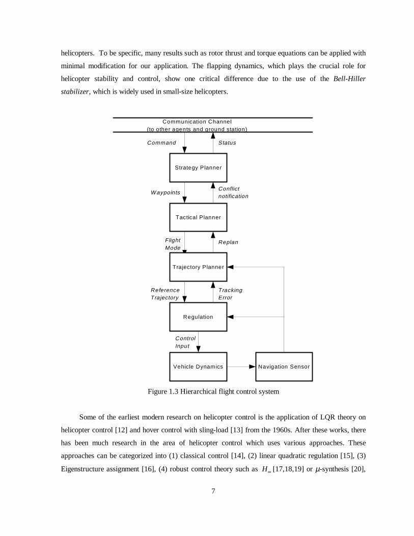
1.2 Hierarchical Vehicle Management Structure

As mentioned above, we are aiming to construct a group of RUAVs that are capable of

performing high-level tasks in an interactive manner. To achieve this level of autonomy, a more

sophisticated approach than simple feedback control is necessary. In this research, we adopt the

hierarchical vehicle management system. This system has been proven very effective for other hybrid

systems problems such as the automated highway system [8] and the air traffic management system

(ATMS) [9](Figure 1.3). The adopted structure allows good insight into how a UAV system should

be constructed as a number of hierarchical layers interacting with each other in order to achieve the

given high-level tasks. When we deal with a hierarchical structure, we can approach it with either a

top-down approach or with a bottom-up approach. While the former advantageously allows a more

systematic and orderly approach, it lacks in perceiving physical requirements and limitations. This

approach often ends up with a total detachment from reality by introducing too many simplifying

assumptions. The irony of idealization is that it yields often mathematically-beautiful-but-just-don’t-

work-in-reality situations. These situations are even more likely to come up when we deal with very

complicated real systems like UAVs. Therefore, the bottom-up approach is chosen because the

problem of UAV system construction is still under vigorous study and hence is not a well-established

area. UAV system construction requires trial-and-error and feedback from the base vehicle

construction problem. Indeed, there have been many instances when we had to go back to the

conceptual design stage to tackle physical problems.

1.3 Relevant Research

There are a number of important fields of science and technology, which are directly related

with this research: (1) general helicopter dynamics, (2) RUAV development, (3) system identification

and (4) control.

Helicopter dynamics have been studied for many decades since its debut in the 1940s. The

helicopter dynamics in theoretical and experimental field are well established [10,11] and it is usually

directly applicable to RUAV study because RUAVs have a very similar configuration to full size

7

helicopters. To be specific, many results such as rotor thrust and torque equations can be applied with

minimal modification for our application. The flapping dynamics, which plays the crucial role for

helicopter stabili ty and control, show one critical difference due to the use of the Bell-Hiller

stabilizer, which is widely used in small-size helicopters.

Vehicle Dynamics

Tactical Planner

Navigation Sensor

Strategy Planner

ReferenceTrajectory

Regulation

ControlInput

Trajectory Planner

FlightMode

Communication Channel(to other agents and ground station)

Command Status

W aypointsConflictnotification

Replan

TrackingError

Figure 1.3 Hierarchical flight control system

Some of the earliest modern research on helicopter control is the application of LQR theory on

helicopter control [12] and hover control with sling-load [13] from the 1960s. After these works, there

has been much research in the area of helicopter control which uses various approaches. These

approaches can be categorized into (1) classical control [14], (2) linear quadratic regulation [15], (3)

Eigenstructure assignment [16], (4) robust control theory such as H∞ [17,18,19] or µ-synthesis [20],

8

and (5) rotor dynamics inclusion [21,22,23] . These results allow insights on how the control system

should be synthesized for small-size helicopter dynamics.

Since the 1980s, a few research results on small-size helicopter control have begun to appear in

publications [24]. During this time, while vast numbers of control theories were available, the

experiments were severely limited by the lack of accurate navigation sensors. As an alternative

approach, they often used a linkage system which is attached to the helicopter body to allow a free but

limited range of motion while providing position and attitude measurements from the potentiometers

installed at each joint [24,25,26,27,28,29]. Usually, the dynamics are additionally constrained to have

freedom in attitude only. This makes the problem easier because the helicopter dynamics in attitude

becomes marginally stable only when the translational motion is constrained [10]. In other research,

ground-based cameras were employed to estimate the position of the helicopter in three-dimensional

space by taking continuous images of the visual markers on the helicopter body. In either case, the

accuracy of motion estimates and the degree-of-freedom of the test vehicle were significantly limited.

After 1990, flying RUAVs in full six degrees-of-freedom and without any constraints or

umbili cal cords finally became possible due to the advent of small-size, high-accuracy INS and GPS.

With this break-through technology, a number of research efforts in similar topics of RUAV

development were published [6,30,31,32]. Another driving force behind RUAV development was the

International Aerial Robotics Competition. This competition has encouraged many research groups to

build autonomous unmanned aerial vehicles designed to perform the given tasks, which require low-

speed or hovering for ground scanning and target recognition.

In this area, Draper Laboratory at MIT, Team Hummingbird of Stanford University, the

Robotics Institute at Carnegie-Mellon University, as well as Georgia Institute of Technology, the

originator of the competition, have participated in the competitions and demonstrated their

technologies of autonomous helicopter systems. Overseas, University of Berlin has been doing

outstanding work for the 1999 and 2000 competitions. It is worthwhile to review how these groups

approached the UAV design problem and understand key technologies they utili zed.

The Hummingbird from Stanford won the competition in 1995 marking the milestone by

demonstrating the first fully autonomous flight and fulf illi ng the rule, which required picking up disks

on one side of a tennis court and dropping them on the other side. The vehicle platform was a hobby-

purpose radio-controlled helicopter, Excel 60, which was heavily modified to carry a total weight of

46 pounds. The unique feature of this helicopter is the sole use of GPS as the navigation sensor. They

wanted to demonstrate that GPS could replace the INS, which is conventionally favored as the

primary navigation sensor. Their GPS system consisting of a common oscill ator and four separate

9

carrier-phase receivers with four antennae mounted at strategic points of the helicopter body provides

the position, velocity, attitude and angular information for vehicle control.

The team from Draper Laboratory won the competition in 1996 by fulfilli ng the new rule,

which required the autonomous vehicle to navigate the given field looking for barrels identifiable by

the labels attached to their top and side and then report the position and type of each barrel to the

ground base. Draper used a 60-class helicopter as their base platform. For the navigation system, they

took the canonical approach of INS/GPS combination. Their navigation system consisted of a

Systron-Donner MotionPak™ IMU, a NovAtel GPS, a digital compass and an ultrasonic altimeter.

The flight computer was a standard PC104 system, which is PC-compatible. The inertial

measurements were sampled and processed by the onboard computer running numerical integration,

the Kalman filtering algorithm, and simple PID control as the low-level vehicle control. The control

gain was determined by tuning-on-the-fly while the safety of the vehicle is at the hand of a very

capable human pilot. The morale of the Draper approach is to demonstrate the possibili ty of building

RUAVs using COTS components.

The winner in the year of 1997 was a group from the Robotics Institute at Carnegie-Mellon

University. They built their RUAV on a Yamaha R-50, a helicopter developed for agricultural use

such as crop-dusting because in Japan because of their tight regulations on the operation of full-size

aircraft. Unlike the previous helicopters, their platform has a more-than-sufficient payload of 20 kg.

The unique feature of their helicopter is the vision-only based navigation capabili ty. The onboard

DSP-based vision processor provides navigation information such as position, velocity and attitude at

an acceptable delay on the order of 10ms. Their vision system is also capable of performing the target

identification required by the same rule as in 1996. Their research is the showcase of an advanced

vision system applied to the aerial vehicle control problem.

1.4 Project History

The Berkeley UAV research group has expanded its scope of interests from the design of a

single UAV flight control system to a group of interacting agents. These agents include UAVs, UGVs

and a ship-motion simulating landing deck. This project first started when our colleague Tak-kuen

John Koo proposed the idea of building an autonomous helicopter system to Professor Shankar Sastry

in the EECS department of UC Berkeley in 1996. He suggested the author to join this project because

of my previous experience with the design and implementation of a hover control for a model

helicopter using LQG/LTR during my Master’s program at Seoul National University in 1991 [26]. In

10

the middle of 1996, the Berkeley UAV team made its humble start by John Koo, Ma Yi, Frank

Hoffman and the author. Our first UAV platform was the Concept 60 SR II f rom Kyosho Industry,

Japan. The 60-class model helicopters are the largest commercially available radio-controlled

helicopters for hobby use and it offers the largest payload without any modification on the powertrain

and rotor blades. Among many helicopters in the 60-class, the Concept 60 from Kyosho Industry was

chosen because of the author’s previous experience with this model. The primary question during this

early period of our research was where this 60-class hobby helicopter could be used for RUAV

platform. The most pressing concern was the payload that this vehicle could handle. With the nominal

output of 2.2 hp of the OS SX-61WC engine, it was observed that it could lift off with 5 kg of

payload and stay in the ground effect region. Without fully understanding that the ground effect can

boost the thrust significantly even up to 200%, it was concluded that the 60-class helicopters could

handle 5 kg of payload or more. It turned out that the acceptable payload of the original 60-class

engine is less than 4kg, which is somewhat less than the desired value of 5-6 kg. The first prototype

was finished in late 1997. Since the symbol of UC Berkeley is a bear, this helicopter was named as

Ursa Minor 1, which means “small bear” in Latin. This helicopter was slated to be the first testbed on

which navigation and control system could be designed and tested. The flight computer system

consists of PC104 compatible CPU and peripheral boards. The navigation system consists of a

NovAtel RT-20 GPS board, a digital compass, and a custom INS system consisting of six

accelerometers positioned in strategic points. The underlying idea of this special INS is that the six

accelerometers can estimate translational acceleration and angular rates using the geometry of the

sensor locations. Unfortunately, the person in charge of this type of INS left our project and a

replacement for INS had to be sought. In early 1998, Systron-Donner MotionPak™ was adopted as

the primary inertial measurement unit. This sensor unit exploits the latest piezoelectric technology

yielding a compact, light-weight, and yet powerful INS solution. It consists of three accelerometers

and three rate gyros in orthogonal configuration and measures the translational accelerations and

angular rates on x, y, and z axis. The raw sensor output, analog voltage from 0V to 10V, is read by an

A/D conversion circuit in the flight computer and then processed to obtain the navigation solution for

identification and control. The inertial navigation integration equation using quaternion was offered

by John Koo and then implemented in MS-DOS and subsequently in QNX. After intense testing for

about a year, it is concluded that the custom INS code lacks a proper sensor bias estimation routine

and cannot be used to obtain a high-accuracy navigation solution. As an alternative solution, John

Koo purchased an INS unit, DQI-NP from Boeing, in late 1998. This INS consists of a piezoelectric

inertial sensor unit and a DSP board to process the inertial measurements at very high rate. The

navigation solution computed by the DSP chip is available on the RS-232 serial port or a custom high

11

speed synchronized serial port. This system allowed the high accuracy navigation estimates and it

boosted to our research progress. The Boeing DQI-NP system is fully integrated with our existing

helicopter platform with substantial modification of the navigation software in early 1999.

The excess payload problem seriously delayed the progress of research since the beginning of

the project. When fully equipped, Ursa Minor 2, the successor of Ursa Minor 1, could not reach an

altitude outside of the ground effect. Many attempts such as using high-lift main rotor blades or high

nitrogen compound composition fuel were made, mostly in vain, to obtain more lift from the same 2-

cycle glow engine with 0.60 cubic inch displacement. The clean answer would be to use a

replacement engine with higher power. This solution, although not impossible, involves redesigning

the engine mount and machining a new gear. These modifications would have exceeded the

capabili ties and resources available to us.

The breakthrough was made by the adoption of a 0.91 cubic inch engine originally designed for

hobby aircraft, with a minor modification of the engine shaft. With this more powerful engine

providing 2.8 hp, Ursa Minor 2 could easily fly out of the ground effect. In parallel to the quest for a

more powerful engine, a larger helicopter platform was also sought. In the middle of 1998, a more

powerful helicopter, Bergen Industrial Twin, joined the Berkeley RUAV fleet. It is equipped with

twin four-stroke gasoline engines welded together for more power. Thanks to this design, the

helicopter offers an available payload of 10kg, which is sufficient for most RUAV applications.

However, a potential structural problem was anticipated because most of the helicopter parts

including the control li nkage and the main rotor grips were originally designed for a 60 class engine

and they would not withstand the excessive loading by the oversized engine. The payload problem

was finally solved by adding Yamaha agricultural helicopters R-50 and their successor RMAX to our

Berkeley UAV fleet. Two Yamaha R-50s arrived at Berkeley in June 1999 and two RMAXs in

December 1999. At the expense of the extremely high cost, the Yamaha helicopters offer high

reliabili ty and generous payload of 20kg-30kg. They now serve as the ultimate platform for diverse

UAV research such as vision-based navigation, dynamic wireless network system and advanced

control law testbeds.

After the two major problems, the INS and the available payload problems, were solved, the

Berkeley BEAR project finally began to see results. In early 1999, a newer version of the Kyosho

helicopter, Concept 60 SR II Graphite, was built as the primary testbed for control system design.

Joining as the third 60-class helicopter, it was named as Ursa Minor 3. Boeing DQI-NP was mounted

at the tip of the nose using special gel-type mounting to minimize the transmission of the severe

engine and rotor vibration. A more powerful CPU, Cyrix MediaGX233, was used in the flight

computer. For GPS, NovAtel Mill enRT-2 was adopted for its unsurpassed accuracy of 2cm. In July

12

1999, this configuration tested on Ursa Minor 3 and then ported to the Yamaha R-50, named as Ursa

Magna.After intensive work during the summer break of 1999, the Ursa Magna 2 was equipped with

a basic navigation suite, a main flight computer and a vision-processing computer. In August 1999,

the first identification flight with active YACS (will be discussed later) was flown. The flight

experiment was performed smoothly and high quality flight data was obtained.

The final breakthrough for the control system was made during October 1999. This time, Ursa

Minor 3 was used again as the main experimental platform because it is easy to manage and repair in

the case of a crash. However, a more adequate mounting could be used with Ursa Magna, thanks to

its size and payload. The result is more stable INS/GPS operation. A similar identification flight,

applying a frequency-sweeping input, was performed during October 1999. The gathered data was

processed using the UAV model proposed by Mettler from Carnegie-Mellon UAV research [7]. The

greatest advantage of his model is the explicit compensation for the Bell-Hill er stabili zer dynamics.

This model was able to predict the stabili zer bar response accurately and the whole model was able to

produce estimates closely matching the flight data. One major difference in the identification process

from the Carnegie-Mellon team was the numerical tool used for the identification process. While they

used the optimization package called CIPHER, which was not available to Berkeley UAV team, I had

to use existing tools such as the MatLAB™ Identification Toolbox™ written by Ljung [34]. While

CIPHER identifies the model in the frequency-domain, the numerical tool offered by Identification

Toolbox™ uses the prediction-error method (PEM) [35]. This approach produced a reasonably

accurate model which is valid for hover. Furthermore, a basic multi-loop controller could be designed

using the classical root-locus method. From late October to late November of 1999, the basic

hovering controller which regulates position in the x, y, and z axis as well as the heading, was

designed. The controller showed superior hovering performance with ±20cm accuracy in the x-y

plane.

Once the basic controller design/implementation/testing was accomplished, the research effort

was steered to the automation of the Yamaha R-50. Many parts of the work for R-50 could be adapted

from Ursa Minor 3 with very minor modifications because they share identical sensors, i.e., Boeing

DQI-NP and NovAtel Mill enRT-2 GPS, and the servomotors accept the same PWM signal.

Differences come from the extended sensor suite such as the ultrasonic height meter, the vision

computer and the ground contact switch sets. As most of the work had been finished in the summer of

1999, only a small amount of modifications and improvements were made in March 2000. One major

difference was the adoption of the Lucent™ (later renamed to Orinoco™) WaveLAN system as the

primary communication device. WaveLAN is a wireless local network device supporting popular

protocols such as TCP/UDP/IP in IEEE 802.11 compatible CSMA/CD format. Before this, a wireless

13

modem with the maximum throughput of somewhere between 57,600-115,200 bps was used for

wireless communication between the ground station and the onboard flight computer. While it offered

reliable performance from the beginning of the project, the radio signal of the wireless modem at 900

MHz might have been strong enough to cause jamming with the NovAtel GPS which is receiving

signals in the 1 GHz band from the GPS satelli tes more than 20,000 km away. On the other hand,

WaveLAN™ trades range with bandwidth. With the new communication system, the ground station

display station, running in Microsoft Window 98, was modified to use the WaveLAN™.

The controller design of the Yamaha R-50 was based on the new system model of this aircraft.

The system model of Yamaha R-50 in hover was identified using a similar approach as was used with

the case of Kyosho Concept 60. This time, a procedure that is more systematic was developed to

identify the model using PEM tool of the MATLAB System Identification Toolbox™. Based on the

identified model, the controller was designed and tested during April to May 2000. The designed

controller for hovering was validated during flight and it showed satisfactory response as is, without

any “tweaking” of the controller gain during the test flight.

During May 2000, a novel concept called Vehicle Control Language (VCL) was conceived for

describing a given mission. As will be discussed later in more detail, VCL is human-understandable

ASCII script-type language, which specifies the helicopter mission at the waypoint level. Different

flight modes such as take-off, hover, turn, cruise and land are specified with coordinates and options

and saved as text files. These VCL files are then uploaded to the target UAV and then executed. The

VCL can be generated by typing the commands or by using the convenient graphical user interface

offered as a part of the ground station program. In July and August 2000, the first-generation VCL

interpreter was tested in a series of test flights and proved the anticipated effectiveness.

1.5 Contributions

This project was funded by Army Research Office (ARO), Office of Naval Research (ONR),

and Defense Advanced Research Project Agency (DARPA). Professor S. Shankar Sastry is in charge

of the whole project. Peter Ray, a staff of Electronics Research Laboratory (ERL) of Electric,

Electronic and Computer Science (EECS) Department of University of California, Berkeley (UCB) is

in charge of financial management. Tak-kuen John Koo, a graduate student of EECS department

proposed, initiated and led the project until 1999. The project was co-founded by Yi Ma, Frank

Hoffman, Kiril Mostov and myself in 1996.

14

The concept of hierarchical structure and hybrid system were contributed by the previous works

of PATH project and ATMS projects. In the beginning, the selection of essential avionic systems was

influenced by the previous works of PATH. With the assist of these works, I achieved the following

works:

• Assembly of Ursa Minor 1 (Kyosho Concept 60 SR-II) (Fall 1996)

• Assembly of Ursa Minor 2 (Kyosho Concept 60 SR-II) (Summer, 1998)

• Assembly of Ursa Minor 3 (Kyosho Concept 60 SR-II Graphite) (Fall 1998)

• Assembly of Kyosho Caliber 60 (Fall 1999)

• Design, fabrication and assembly of avionics electronics for Ursa Minor 1 (Fall 1997)

• Design, fabrication and assembly of avionics electronics for Ursa Minor 2 (1998)

• Design, fabrication and assembly of avionics electronics for Ursa Minor 3 (Spring

1999)

• Design, fabrication and assembly of avionics for Ursa Magna 2 (Yamaha R-50)

(Summer 1999~)

• Design and partial assembly of the avionics for Ursa Maxima 2 (Yamaha RMAX)

(Summer 2000~)

• Mechanical part design of tail servo mounting, custom IMU mounting, GPS mounting,

etc

• Mounting and enclosure design and machining for Ursa Minor 1, Ursa Minor 2, Ursa

Minor 3, Ursa Magna 2 and partial work on Ursa Maxima 3

• Circuit design, layout and fabrication of custom take-over board (TOB) for Ursa Minor

1, Ursa Minor 2, Ursa Minor 3, and Ursa Magna 2

• Programming for early version of navigation algorithm in MS-DOS and QNX

• System identification of Ursa Minor 3 and Ursa Magna 2

• Simulation model derivation and programming in MATLAB/Simulink for Ursa Minor

2, Ursa Minor 3, and Ursa Magna 2

• Classical multi-loop controller design for Ursa Minor 3 and Ursa Magna 2

• µ-Synthesis controller design for Ursa Minor 2 and Ursa Magna 2

• Design, programming, and testing of vehicle management software (VMS) for Ursa

Minor 2 (December 1998~April 1999)

• Design, programming, and testing of VMS for Ursa Minor 3 (April 1999~March 2000)

• Design, programming, and testing of VMS for Ursa Magna 2 (June 1999~)

15

• Design, programming, and testing of VMS for Ursa Maxima 2 (May 2000~)

• Integration of INS/GPS using Systron-Donner MotionPak IMU and NovAtel GPS

Mill enRT-2 for Ursa Minor 2 (June 1998~April 1999)

• Integration of INS/GPS using Boeing DQI-NP INS and NovAtel GPS Mill enRT-2 for

Ursa Minor 3 and Ursa Magna 2 (January 1999~)

• Identification flight of Ursa Minor 3 (October 1999)

• Test flight of Ursa Minor 3 (October 1999~March 2000)

• Test flight of Ursa Magna 2 (March 2000~current)

• Creation, programming, simulation, and test flight of VCL-based waypoint navigator

(May 2000~)

John Koo is responsible for the shaping-up of the project from the beginning to summer 1999.

Willi am Morrison, a graduate student in Mechanical Engineering (ME), designed and machined the

mounting of an INS, ultrasonic sensor mounting, battery tray, avionics mounting, and contact switch

fixture of Ursa Magna 2.

Santosh Philli p (ME) wrote the driver for Senix ultrasonic sensor.

Shahid Rashid (EECS) and Santosh Philli p wrote a TCP/IP driver for QNX. Shahid also wrote

a GUI using LabWindows®.

Cedric Ma (EECS) wrote OpenGL-based software for three-dimensional visualization of

helicopter control simulation results. He also performed the system identification test flight of Ursa

Magna 2 twice (one time with YACS on and the other time with YACS off).

Hoam Chung (ME) fabricated the majority of the avionics of Ursa Maxima 2. He also assisted

many important flight tests such as waypoint navigation and µ-Synthesis attitude controller on Ursa

Magna 2 since June 2000.

While not introduced in detail i n this dissertation, the vision system and the UGV system are

related with this work. Omid Shakernia (EECS), Cory Sharp (EECS), and Rene Vidal (EECS) are

responsible for the color tracking vision system on Ursa Magna 2 and UGVs. Cory Sharp wrote the

guidance software for Pioneer outdoor UGVs and developed, programmed, and tested a special vision

algorithm on Ursa Magna 2. Tulli o Celano III (US Navy) constructed two ship-motion simulators

based on Stuart platform: the earlier version with electric motors (Fall 1999) and the later and larger

version with hydraulic cylinders (Winter 1999~2000). A number of joint works were performed with

them: the semi-automatic landing with Ursa Minor 3 (December 1999) and color-based UGV tracking

with Ursa Magna 2 (August 2000).

16

1.6 Scope of This Dissertation

The research presented in this dissertation finds its significance in the establishment of a systematic

methodology for the development of RUAVs by the use of commercial off-the shelf (COTS)

components such as radio-controlled helicopters, navigation sensors, computers, and communication

devices. With the ultimate goal of fully autonomous flight capabili ty from take-off to landing, each

step towards the goal has been developed, implemented and tested on three RUAVs. These steps are

(1) helicopter dynamics modeling, (2) parametric system identification, (3) hardware integration, (4)

software design, and (5) flight test. In the following chapters, the developed technologies for these

stages are presented.

The helicopter model is derived from a general full-size helicopter model with the

augmentation of the servorotor dynamics. The acquired nonlinear model is directly used for

simulation model and it is further simplified through linearization in order to obtain a linear model for

controller design. Helicopter platforms are integrated with navigation sensors and onboard flight

computers. Once the hardware and software are ready, a number of identification flights, manual

flights with certain inputs exciting each flight mode of roll, pitch, yaw and heave, were flown. The

input and output of the helicopter was sensed, sampled, downloaded and recorded for processing. The

parametric helicopter model for hover is identified by running an identification algorithm with the

collected data. After a high-fidelity model was found, both classical control theory and state-space

based linear robust control theory are applied for helicopter stabili zation. The proposed controllers

were tested on Berkeley RUAVs and they showed satisfactory results.

Based on the successful controller for the low-level vehicle stabili zation, a vehicle guidance

logic is developed. A unique approach proposed in this research is the novel concept of Vehicle

Control Language (VCL). VCL is a middle-level vehicle guidance layer in the hierarchical structure

shown in Figure 1.3. This approach provides the isolation and abstraction between the low-level

vehicle control and the mission-level condition. In this framework, the onboard autopilot system can

perform any given feasible mission without any reprogramming of onboard software as the mission

changes. The sequence of motion commands is described in a script language form understandable to

humans. The VCL module consists of a user interface part on the ground station, a language

interpreter, and a sequencer on the UAV side.

It should be stressed that all of the proposed idea in this dissertation were fully tested repeatedly

in the actual flight tests. From this point, it is asserted that all of the proposed methodologies in this

paper can be repeated on the other RUAV platforms with proper minor modifications.

17

This dissertation is organized in the following order: in Chapter 2, the general helicopter

dynamics are overviewed and the nonlinear simulation model and linear control model are

established. Chapter 3 introduces the hardware and software implementation of Berkeley RUAVs in

detail. In Chapter 4, the autopilot system design in the context of multi-layer hierarchical structure is

addressed. For the low-level control, two distinct approaches of classical control and modern linear

robust control are applied for the design of the stabili zing controller using the system model identified

in Chapter 2. To bridge the low-level vehicle regulation layer and the high-level strategic

coordination, the novel approach of Vehicle Control Language is introduced and the experiment

results are shown. Detailed technical information about the RUAVs used in this research is given in

the Appendix.

18

Chapter 2

2. Helicopter Dynamics Modeling and

System Identification

To design an effective autopilot system for a RUAV system, we should first understand the

dynamics of the target vehicle platform. The helicopter dynamics are derived by establishing the

equations of motion by aerodynamic analysis of the whole system. The dynamics of the helicopter

have been well studied over decades and abundant theoretical as well as experimental results are

available [10,11]. A nonlinear model to our best knowledge is desired for high-fidelity simulations

upon which the proposed controllers are validated. For controller design, the model may be simplified

to the detail l evel that the applied control theory requires

Helicopter dynamics are nonlinear, inherently unstable, coupled, input-saturated, MIMO, and

time-varying system with changing parameters. It is exposed to unsteady disturbances such as wind

gust and cross wind while operating in diverse flight modes such as take-off, landing, hover, forward

flight, bank-to-turn, and even inverted flight. Due to the complicated and almost chaotic behavior

involved with the aerodynamics of a helicopter, it is virtually impossible to obtain fully accurate

dynamic equations valid for all the aforementioned flight modes. Theoretical model often has rather

large errors and has to be adjusted with the experimental data. Therefore, we often have to

compromise to obtain models with moderate accuracy for simulation and control design.

In this chapter, we first briefly overview the coordinate systems that are used as the reference

frame for the description of helicopter motion. Then, we develop a fully nonlinear model of the

helicopter dynamic by lumped-parameter approach. The results derived for full-size helicopters are

adapted to account for the specific dynamic behavior of the servorotor of small-size helicopters. The

19

general dynamics are simplified to a model valid for hover and low-velocity motion. The theoretical

model derived by aerodynamic equations oftentimes include rather large error due to the inaccurate

knowledge about the actual parameters of aerodynamic components and has to be reconciled with the

actual experimental results. This process requires certain experiment facili ties such as wind tunnel or

whirl tower. In many cases, however, these facili ties are not easy to access and it would take

tremendous time and effort for a small research group in a university. Therefore, we are forced to find

some other way to find a model for controller design. For this reason, we adopt the parametric linear

time-invariant model proposed by Mettler [7] and seek to identify the parameters in the model using

the flight data from our RUAVs.

2.1 Coordinate Systems and Transformations

A number of coordinate systems are introduced to describe the motion of RUAV in three-

dimensional space.

• Inertial reference system

• Earth-Centered Earth-Fixed (ECEF) system

• Tangent-plane coordinate system

• Body-coordinate system

2.1.1 Inertial Reference System and ECEF System

The inertial reference system is the hypothetical coordinate system where the classical

Newtonian mechanics is assumed to hold true. For describing motion bound to the Earth, the inertial

reference system is not very convenient because the Earth rotates with respect to the inertial frame. In

this application, the ECEF coordinate system, which is not an inertial reference frame, is more

convenient. The ECEF coordinate system is, as the name implies, attached to the center of the earth

and rotates together as the Earth rotates. Hence, any fixed geographical location on the Earth has

constant coordinates with respect to the ECEF system. In the ECEF coordinate system, a given point

is expressed in either Cartesian coordinates or geodetic coordinates. The coordinate in the ECEF

system is specified by ( , , )e e ex y y in the Cartesian coordinate system. The geodetic coordinate system

employs certain hypothetical elli psoid to approximate the complex surface shape of the Earth. A

20

geodetic elli psoid is defined by its semimajor axis length (a), eccentricity (e), inertial rate of rotation

( ieω ), and equatorial effective gravity ( eγ ) [36]. There are a number of standard elli psoids and hence

it should be specified when the geodetic coordinates are used in literature. For now, the WGS-84

elli psoid is commonly used in literature for describing the operation of INS and GPS. In WGS-84

standard, the semimajor and semiminor axes are defined as

Semimajor axis length: a=6378137.0 m

Semiminor axis length: b=6356752.3142 m

In the geodetic system, a coordinate is described by latitude, longitude and absolute height, i.e.,

( , , )ehλ φ . There is a transformation relationship between the Cartesian coordinates and geodetic

coordinates. In WGS-84 standard, the flatness of the elli psoid is defined as

0.0034a b

fa

−= = (2.1)

The eccentricity of the elli psoid is defined as

(2 )e f f= − (2.2)

The length of the normal to the elli psoid, from the surface of the elli psoid to its intersection

with the ECEF z-axis, is

2 2

( )1 sin

aN

eλ

λ=

− (2.3)

With given ( , , )ehλ φ and f, e, and N (2.1), (2.2) and (2.3), the Cartesian coordinates are found

by the following equations.

( )cos cosx N h λ φ= + (2.4)

( )cos siny N h λ φ= + (2.5)

2[ (1 ) ]sinz N e h λ= − + (2.6)

The transformation in the other direction, i.e., geodetic to Cartesian, is rather complicated but

exists as well [36].

21

Φ

λ λ

Equator

PrimeM eridian Geodetic

Ellipse

a

b

N

h

z

eX

eY

eZ

Figure 2.1 Geodetic reference coordinate system

2.1.2 Tangent Plane Coordinate System

The tangent-plane frame is also called the local Cartesian coordinate system. Its origin is

located on a certain point of interest and its x, y, z axes align respectively with the north, east and

downward direction of the ECEF frame (Figure 2.2). In localized navigation, other than global-scale

navigation, it is often more convenient to refer to this coordinate system than geodetic coordinates or

Cartesian coordinates in the ECEF frame. Since GPS measurements refers to the ECEF coordinate,

we need a transformation from ECEF to the tangent plane coordinate system as following.

Φ

λ

Equator

local tangent plane

eX

eY

eZ

tpy

tpx

tpz

Figure 2.2 Tangent plane coordinate system

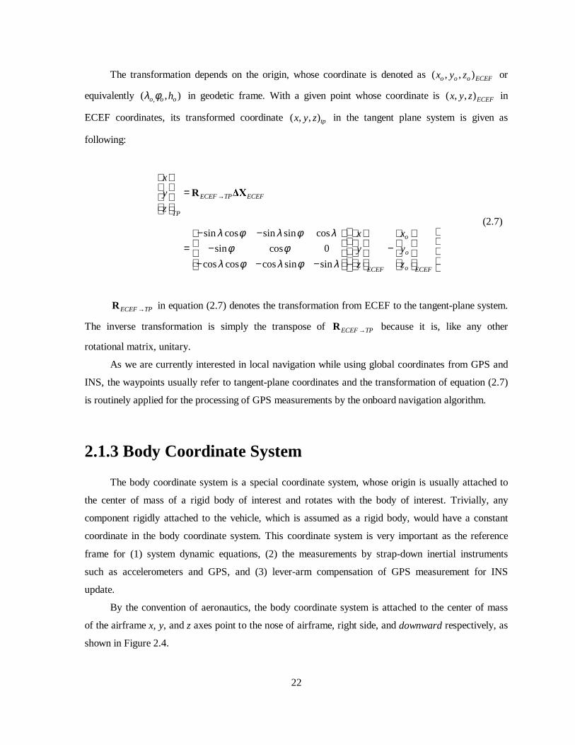
22

The transformation depends on the origin, whose coordinate is denoted as ( , , )o o o ECEFx y z or

equivalently ,( , )o o ohλ φ in geodetic frame. With a given point whose coordinate is ( , , )ECEFx y z in

ECEF coordinates, its transformed coordinate ( , , )tpx y z in the tangent plane system is given as

following:

sin cos sin sin cos

sin cos 0

cos cos cos sin sin

ECEF TP ECEF

TP

o

o

oECEF ECEF

x

y

z

x x

y y

z z

λ φ λ φ λφ φ

λ φ λ φ λ

→

=

− − = − − − − −

R û;

(2.7)

ECEF TP→R in equation (2.7) denotes the transformation from ECEF to the tangent-plane system.

The inverse transformation is simply the transpose of ECEF TP→R because it is, like any other

rotational matrix, unitary.

As we are currently interested in local navigation while using global coordinates from GPS and

INS, the waypoints usually refer to tangent-plane coordinates and the transformation of equation (2.7)

is routinely applied for the processing of GPS measurements by the onboard navigation algorithm.

2.1.3 Body Coordinate System

The body coordinate system is a special coordinate system, whose origin is usually attached to

the center of mass of a rigid body of interest and rotates with the body of interest. Trivially, any

component rigidly attached to the vehicle, which is assumed as a rigid body, would have a constant

coordinate in the body coordinate system. This coordinate system is very important as the reference

frame for (1) system dynamic equations, (2) the measurements by strap-down inertial instruments

such as accelerometers and GPS, and (3) lever-arm compensation of GPS measurement for INS

update.

By the convention of aeronautics, the body coordinate system is attached to the center of mass

of the airframe x, y, and z axes point to the nose of airframe, right side, and downward respectively, as

shown in Figure 2.4.

23

The transformation between the body coordinate system and the tangent plane system is also

needed. This transformation involves the translation and rotation of the rigid body representation of

airframe with respect to the tangent plane reference coordinate system. In vector geometry, any point

on the rigid body, denoted by TPX , can be represented by vector sum as shown in the following:

P O O PTP TP TP

O O PTP B TP B

→

→→

= +

= +

X X X

X R X (2.8)

There are three representations for the rotation transformation B TP→R .

2.1.3.1 Euler Angles

The rotational matrix commonly represented by the Euler angle of (roll, pitch, yaw), denoted by

( , , )Φ Θ Ψ , respectively, is given as:

cos cos sin cos sin

sin cos cos sin sin cos cos sin sin sin cos sin

sin cos cos sin cos cos sin sin sin cos cos cos

B TP→

Ψ Θ Ψ Θ − Θ = − Ψ Φ + Ψ Θ Φ Ψ Φ + Ψ Θ Φ Θ Φ Ψ Φ + Ψ Θ Φ − Ψ Φ + Ψ Θ Φ Θ Φ

R

(2.9)

Again, the transformation B TP→R is unitary and the inverse transformation is simply

1 TTP B B TP B TP

−→ → →= =R R R (2.10)

Another important equation is the differential equation relating (p, q, r), the angular rates in the

x, y, and z direction, with the Euler angle ( , , )Φ Θ Ψ :.

1 sin tan cos tan

0 cos sin

0 sin / cos cos / cos

pd

qdt

r

Φ Φ Θ Φ Θ Θ = Φ − Φ Ψ Φ Θ Φ Θ

(2.11)

24

The inertial navigation algorithm can compute the attitude of the vehicle by solving the

differential equation (2.11). It should be noted, however, that the matrix has singularity at 90Θ = ± ° ,

when the vehicle is upside down. In normal operation of the helicopter, this is not a serious problem,

but it can still pose serious limitations in some cases. Indeed, small-size hobby helicopters are capable

of hovering upside down. While the Euler angle representation is intuitively appealing and convenient

for dynamic equations, representations without any singularities, such as direction-cosine or

quaternion, are preferred for the implementation of INS.

2.1.3.2 Quaternion Representation

Quaternion parametrization is a favored method to represent the rotation of a rigid body

because it is free from singularities and it is computationally efficient. A quaternion is a vector of four

entities obeying generalized complex algebraic rules:

1 2 3 4q q q q= + + +q i j k (2.12)

where

1

1 1 1

=

= − = − = −= = =

= − = − = −

q

i i j j k k

i j k j k i k i j

j i k k j i i k j

D D D

D D D

D D D

A quaternion is equivalently represented by a vector: [ ]1 2 3 4T

q q q q=q .

The angular motion is described entirely by the quaternion representation as shown below:

4 3 2

3 4 1

2 1 4

1 2 3

0

01

02

0

1

2

r q p

r p q

q p r

p q r

q q qp

q q qq

q q qr

q q q

=

− − = − − − −

− − = − − − −

q T

q

(2.13)

25

Obviously, integrating equation (2.13) is much more efficient than (2.11) because it does not

involve computationally expensive trigonometric functions. The rotational transformation matrix

B TP→R can be directly found with quaternion:

2 2 2 21 4 2 3 1 2 3 4 1 3 2 4

2 2 2 21 2 3 4 2 4 1 3 2 3 1 4

2 2 2 21 3 2 4 2 3 1 4 3 4 1 2

2( ) 2( )

2( ) 2( )

2( ) 2( )

B TP

q q q q q q q q q q q q

q q q q q q q q q q q q

q q q q q q q q q q q q

→

+ − − − +

= + + − − − − + + − −

R (2.14)

The major advantage of using quaternion is, although it is not intuitive at all, the computational

efficiency and the absence of the singularities that the Euler angles have. In some situations, vehicle

feedback control for example, Euler angles are still necessary and the relationship is given as follows:

2 4 1 3

2 22 3 1 4 1 2

2 21 2 3 4 2 3

sin 2( )

arctan2 2( ), 2( )

arctan2 2( ), 2( )

q q q q

q q q q q q

q q q q q q

Θ = − +

Φ = − − +

Ψ = − − +

(2.15)

2.1.3.3 Direction Cosine

The direction cosine matrix is widely used in aerospace applications, especially in the design of

inertial navigation systems [37]. Any two vectors in three-dimensional space, denoted by 1r and 2r ,

intersect with angle θ , which can be found by the inner product relationship:

1 1 2

1 2

cosθ − =

r rr rD

(2.16)

Suppose there are two coordinate systems, denoted by superscript a and b. A vector X can be

represented by two coordinate systems a and b denoted by aX and bX , respectively. There exists a

unique transformation between these two coordinate systems satisfying

b b aa=X R X (2.17)

26

The transformation can be found by the following idea. We can find the intersection angles

among the orthogonal unit vectors of two frames, denoted by ( ), ,a a ax y zi i i and ( ), ,b b b

x y zi i i , and then cast

into the matrix form

b a b a b ax x x y x z

b b a b a b aa y x y y y z

b a b a b az x z y z z

=

i i i i i i

R i i i i i i

i i i i i i

D D D

D D D

D D D

(2.18)

In fact, the transformation matrix (2.18) is the identical rotational matrix presented earlier in

equation (2.9).

Another important relationship is the time derivative of the transformation matrix (2.18). The

transformation matrix changes as a function of time when the vehicle rotates as a function of time

with respect to the inertial frame. The derivative can be found by

3 2

3 1

2 1

( )

0

0

0

bb baa ab

ba

d t

dt

ω ωω ωω ω

=

− = − −

RR

R

(2.19)

bab denotes the angular change of the b-frame relative to the a-frame, coordinatized in the b-

frame. Note that the skew-symmetric matrix bab can be represented by a vector

1 2 3[ ]Tω ω ω=& with outer-product operator.

When & is constant, the solution of the differential equation (2.19) is

( )

0

2

0 2

( ) ( )exp( )

sin 1 cos( )

b b ba a ab

b b ba ab ab

t t t

t tt

=

− = + +

R R

& &R I

& &

(2.20)

The rotational matrix at every time t may be found by calculating the solution (2.20).

Comparing the dual approaches, it is known that the quaternion approach is numerically efficient and

yields lower error solutions [36].

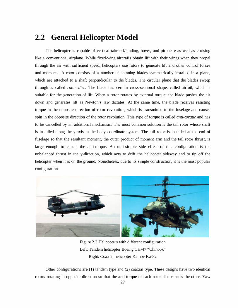
27

2.2 General Helicopter Model

The helicopter is capable of vertical take-off/landing, hover, and pirouette as well as cruising

like a conventional airplane. While fixed-wing aircrafts obtain lift with their wings when they propel

through the air with sufficient speed, helicopters use rotors to generate lift and other control forces

and moments. A rotor consists of a number of spinning blades symmetrically installed in a plane,

which are attached to a shaft perpendicular to the blades. The circular plane that the blades sweep

through is called rotor disc. The blade has certain cross-sectional shape, called airfoil, which is

suitable for the generation of lift. When a rotor rotates by external torque, the blade pushes the air

down and generates lift as Newton’s law dictates. At the same time, the blade receives resisting

torque in the opposite direction of rotor revolution, which is transmitted to the fuselage and causes

spin in the opposite direction of the rotor revolution. This type of torque is called anti-torque and has

to be cancelled by an additional mechanism. The most common solution is the tail rotor whose shaft

is installed along the y-axis in the body coordinate system. The tail rotor is installed at the end of

fuselage so that the resultant moment, the outer product of moment arm and the tail rotor thrust, is

large enough to cancel the anti-torque. An undesirable side effect of this configuration is the

unbalanced thrust in the y-direction, which acts to drif t the helicopter sideway and to tip off the

helicopter when it is on the ground. Nonetheless, due to its simple construction, it is the most popular

configuration.

Figure 2.3 Helicopters with different configuration

Left: Tandem helicopter Boeing CH-47 “Chinook”

Right: Coaxial helicopter Kamov Ka-52

Other configurations are (1) tandem type and (2) coaxial type. These designs have two identical

rotors rotating in opposite direction so that the anti-torque of each rotor disc cancels the other. Yaw

28

motion is obtained by controlli ng the difference of the anti-torque of each rotor. Coaxial-rotor

helicopters have two main rotors attached to a coaxial shaft rotating in opposite directions. This

approach results in a shorter body without a tail boom at the expense of a very complicated power

transmission and control structure of the main rotor. Tandem helicopters, take the Boeing CH-47 for

example, have two identical rotors rotating in opposite direction on the front and the rear top of the

fuselage.

All of the Berkeley UAV fleet, i.e., Kyosho Concept 60 SR II, Bergen Industrial Twin, Yamaha

R-50 and RMAX, have the configuration of one-main-rotor and one-tail-rotor, which was pioneered

by Igor Sikorsky in the 1940s. In the following, we concentrate on the dynamics of main-tail rotor

configuration helicopters.

2.2.1 Kinematic-Dynamic Equation of the Helicopter

The motion of a rigid body in three-dimensional space is characterized by the position TPX of

the center of mass and the Euler angles ( , , )Φ Θ Ψ for rotation of the helicopter with respect to the

tangent-plane frame. In the following formulation, we employ the tangent plane coordinate system as

the inertial reference frame by neglecting the rotation of the Earth. The rigid body obeys the

following kinematic equations:

TP TP=X V (2.21)

1 sin tan cos tan

0 cos sin

0 sin / cos cos / cos

bd

dt

Φ Φ Θ Φ Θ Θ = Φ − Φ Ψ Φ Θ Φ Θ

& (2.22)

where

3TTP TP TP TPx y z ∈ X 5

TPV : velocity of center of mass in the tangent plane frame

Helicopter dynamics obey the Newton-Euler equation for rigid body in translational and

rotational motion. The dynamic equation is conveniently described with respect to the body

coordinate system.

1b b b

extm= − ×V F & 9 (2.23)

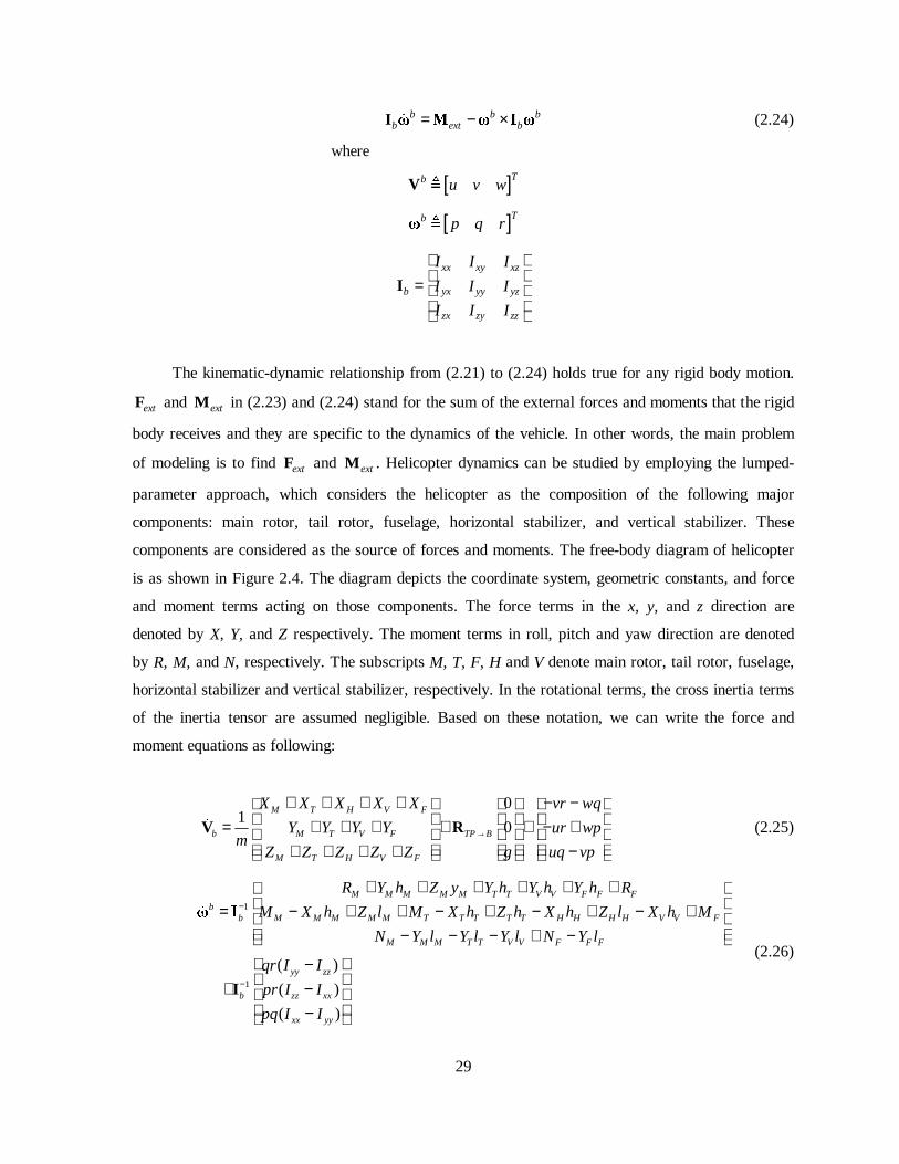
29

b b bb ext b= − ×I & 0 & , & (2.24)

where

[ ]Tb u v wV

[ ]Tb p q r&

xx xy xz

b yx yy yz

zx zy zz

I I I

I I I

I I I

=

I

The kinematic-dynamic relationship from (2.21) to (2.24) holds true for any rigid body motion.

extF and extM in (2.23) and (2.24) stand for the sum of the external forces and moments that the rigid

body receives and they are specific to the dynamics of the vehicle. In other words, the main problem

of modeling is to find extF and extM . Helicopter dynamics can be studied by employing the lumped-

parameter approach, which considers the helicopter as the composition of the following major

components: main rotor, tail rotor, fuselage, horizontal stabili zer, and vertical stabili zer. These

components are considered as the source of forces and moments. The free-body diagram of helicopter

is as shown in Figure 2.4. The diagram depicts the coordinate system, geometric constants, and force

and moment terms acting on those components. The force terms in the x, y, and z direction are

denoted by X, Y, and Z respectively. The moment terms in roll, pitch and yaw direction are denoted

by R, M, and N, respectively. The subscripts M, T, F, H and V denote main rotor, tail rotor, fuselage,

horizontal stabili zer and vertical stabili zer, respectively. In the rotational terms, the cross inertia terms

of the inertia tensor are assumed negligible. Based on these notation, we can write the force and

moment equations as following:

01

0M T H V F

b M T V F TP B

M T H V F

X X X X X vr wq

Y Y Y Y ur wpm

Z Z Z Z Z g uq vp→

+ + + + − − = + + + + + − + + + + + −

V R (2.25)

1

1

( )

( )

( )

M M M M M T T V V F F Fb

b M M M M M T T T T T H H H H V V F

M M M T T V V F F F

yy zz

b zz xx

xx yy

R Y h Z y Y h Y h Y h R

M X h Z l M X h Z h X h Z l X h M

N Y l Y l Y l N Y l

qr I I

pr I I

pq I I

−

−

+ + + + + + = − + + − + − + − + − − − + − − + − −

& ,

I

(2.26)

30

Side View

Top View

Rear View

MhFh

VhThHl

HX

Hh

FMFX

MX MM

FlFZ HZ

Θ

Horizon

mgZ

X

MZ

VX

TX

TZ

TM

X

Y

ReferenceHeading

FYMY

MNFN

VYTY

Vl

Tl

Ψ

FlMl

Y

Z

Φ

MZ

My

MR

MYMh

ThVh

Fh

TY

VY

FYFR

Figure 2.4 Free body diagram of helicopter with respect to body coordinate system

Now the problem reduces to the formulation of each force and moment term and the

measurements of the geometric constants specific to the location of center of mass and the location of

main rotor, tail rotor, and stabili zer fins. In the following sections, we seek to find the equations for

each force and moment term following the results by Prouty [10]. This is not a trivial task because the

aerodynamics involved are very complicated and the resulting equations may be in implicit form

and/or involve look-up tables and graphs. The overall accuracy may fall below the demanded

accuracy. Still , this process is valuable to gain insight of the overall helicopter dynamics, which are

helpful to design control systems and operate the vehicle. Once we finish finding these terms, we can

construct a simulation model and a control model.

31

2.2.2 Main Rotor

The main rotor is the most crucial part of the helicopter dynamics. It generates the vertical

thrust, or lift, to act against gravity. The main rotor system is also the most complicated mechanical

part of the entire helicopter system. A main rotor typically has two to six blades in radial

configuration separated by an equal angle. A blade is bolted to the blade grip, which is attached to the

main rotor head through a bearing system (articulated) or strap (hingeless). The lift generated by the

blade is the function of many factors including relative air speed, air density, airfoil shape, angle-of-

attack and so forth. The main rotor system also has a mechanism called swashplate which changes the

blade pitch simultaneously or as the function of the angular position of the main rotor shaft. The

former is called collective pitch and the latter is called cyclic pitch. The collective pitch changes the

pitch of all blades to control vertical li ft. The cyclic pitch changes the distribution of the lift force

over the disc so that the direction of the thrust vector can be tilted from the upright direction. It also

generates rolli ng and/or pitching moment to cause the fuselage to tilt and the inclination in roll and/or

pitch induces lateral and/or longitudinal motion respectively.

The dynamic equation of the main rotor can be obtained by an analysis called blade-element

method [10]. It starts with the analysis of an infinitesimal blade element on which various forces such

as lift, drag, and centrifugal force act. The overall dynamics of the main rotor can be found by

integrating the force and moment terms along the blade length.

In Figure 2.5, the geometry and the free-body diagram for the blade element method is given.

The lift generated on the blade element is a function of the local dynamic pressure, lift coefficient and

the width of the blade.

iL qcc r∆ = ∆ (2.27)

where q : local dynamic pressure

ic : local li ft coefficient

c : width of blade

The local dynamic pressure q and the local li ft coefficient ic are given by

( )212

q rρ= Ω (2.28)

ic aα= (2.29)

where ρ : air density

32

Ω : angular velocity of rotor

a : slope of the lift curve

α : local angle of attach

With the given geometry in Figure 2.5, the following relationships are found:

α θ φ= − (2.30)

1 1 1tanv v

r rφ −=

Ω Ω (2.31)

(a)Geometry of a Blade Element

iD∆

L∆φ

θ

1v φ

α

rΩoD∆

(b) Free body diagram of blade method

Figure 2.5 Blade element method

33

The total thrust of the rotor can be found by the following integration

0

2 2 1( )

2

R

R

v rT bL abc r r dr

ρ θ = = Ω − Ω ∫ (2.32)

1v in equation (2.32) is the induced velocity of air volume pushed down by the revolving blade.

It is a function of r. In hover, when there is no additional relative air speed from horizontal or vertical

velocity, it has the implicit form with the thrust T:

2

1 2 2 2c cV V T

vAρ

= − + + (2.33)

where cV : climb velocity of the rotor

Note that 1v in equation (2.33) is in fact the averaged induced velocity of the rotor disc and it

yields approximated results when solved in an iterative manner [11] or in closed form after certain

manipulation [26]. For more accurate analysis, the following equation for 1v as the function of r is

used.

22

1

4 4 82 2

( )8

cc c

Vabc V abc V abc r

rv r

π π π θ

π

Ω Ω − + + + + Ω − Ω = (2.34)

Plugging equation (2.34) into (2.32), after a long manipulation, T in closed form is given as

follows with some constant variables introduced for simplicity in manipulation:

( )

( )( ) ( )( )( )3 32 2

2

3 32 20 3 6

3 0

32 5 2 5 2 0 5 2 0 52 2 2

3 2

23 2 3 2

8 15

R R m mT m R R

mm R m m R m m R m m R m

m

θ

θ θ θ θπ θ

−= + −

− − + − − + Ω

(2.35)

where

34

1

22

23

2 25 1

16

42

8

2

1

8

c

c

c

m abc V

m abc

m abc

V mm m

mm V

π

π

ρ

π

Ω= +

= Ω

= Ω

= −Ω

= − Ω

(2.36)

As obvious in equation (2.35) and (2.36), T is a function of many geometric parameters: the

main rotor (b, c, R 0R ), the aerodynamic parameters of the blade ( ρ , a) and the operational

parameters (, ,cVθ Ω ). Once the rotor geometry is determined, then the rotor thrust can be controlled

by the collective pitch θ and the rotor RPM Ω . As mentioned earlier, full-size helicopters have an

engine governor to regulate the rotor RPM to a constant speed. Small size helicopters usually do not

have the luxury of a governor. Instead, the radio controller has special mixing capabili ty to

simultaneously control the collective pitch and the engine throttle opening in preprogrammed

mapping so that the engine can keep up with the varying load by the rotor. Since this mapping is

preset, the engine RPM does fluctuate upon the change of the load on the engine. This method does

not impose too much difficult y on human pilots. For automatic control, the engine governor is desired

to keep the helicopter dynamics less perturbed for model-based controllers. In our research, engine

governors are built using an optical encoder, which picks up the difference of reflectivity of a marker

on the flywheel. The engine governor for hobby purpose (Futaba GV-1) is also available.

Another important contribution of main rotor is the torque Q, which can be computed by the

similar blade element approach. As can be seen in the free-body diagram in Figure 2.5, there are two

sources of horizontal drag force, induced drag and profile drag, whose outer product with the moment

arm r acts as the anti-torque:

( )Q L D rφ∆ = ∆ + ∆ (2.37)

The induced drag is the horizontal component of the lift, which is perpendicular to the direction

of local flow. The profile drag is the air resistance force parallel to the local flow. Substituting the

expression for L∆ and D∆ , equation (2.37) becomes

35

( ) ( )2 2

2 2l cQ r r c c r r c c rρ ρφ ∆ = Ω ∆ + Ω ∆

(2.38)

After substituting (2.31) and (2.34) into (2.38), and enormous manipulation, we obtain Q:

( )( )

( )( )

( )

( )( ) ( )( )

( )

32

32

3 32 2

3 30

1 7

2 2 21 84 4 5 5 4 53

4

2 2 24 0 4 5 0 5 4 0 5

3 31 90

1 104 5 4 5 4 0 5 4 0 53

4

4 410

3

215 12 8

105

15 12 8

2

23 2 3 2

15

4

d

R RQ n n

n nm R m mR m m R m

m

m R m mR m m R m

n nR R

n nm R m m R m m R m m R m

m

c nR R

−=

+ − + +

− − + +

− − +

− + − − +

+ −

(2.39)

where

( )

21

12

3 2

24 1 5

5 2

2

8

8

4

c

c

n bc

mn V

an

n m m

aVn

ρ

π

π

π

= Ω

= −

=Ω

= +

=Ω

2

6

7 2 3 4

8

9 3 4 5 1 6

10 1 3 5

8

2

cVn a

an n n m

an

n n n n m n

n mn n

θ

θπ

= Ω

= −Ω

=Ω

= − +

= −

(2.40)

Closed-form equations with rather overwhelming complexity have been derived. One

discouraging aspect of this approach is that aerodynamic equations usually contain 5~20% error due

to the imperfect knowledge of the involved aerodynamic quantities and the chaotic nature of fluid

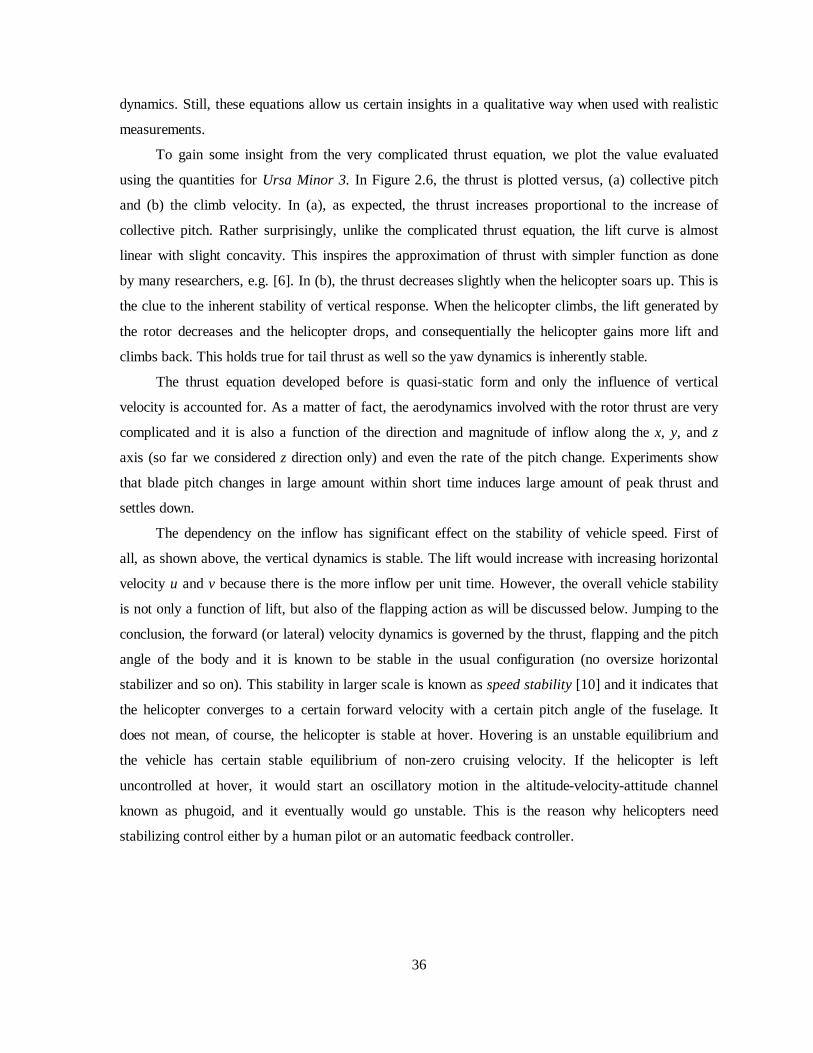
36

dynamics. Still , these equations allow us certain insights in a qualitative way when used with realistic

measurements.

To gain some insight from the very complicated thrust equation, we plot the value evaluated

using the quantities for Ursa Minor 3. In Figure 2.6, the thrust is plotted versus, (a) collective pitch

and (b) the climb velocity. In (a), as expected, the thrust increases proportional to the increase of

collective pitch. Rather surprisingly, unlike the complicated thrust equation, the lift curve is almost

linear with slight concavity. This inspires the approximation of thrust with simpler function as done

by many researchers, e.g. [6]. In (b), the thrust decreases slightly when the helicopter soars up. This is

the clue to the inherent stabili ty of vertical response. When the helicopter climbs, the lift generated by

the rotor decreases and the helicopter drops, and consequentially the helicopter gains more lift and

climbs back. This holds true for tail thrust as well so the yaw dynamics is inherently stable.

The thrust equation developed before is quasi-static form and only the influence of vertical

velocity is accounted for. As a matter of fact, the aerodynamics involved with the rotor thrust are very

complicated and it is also a function of the direction and magnitude of inflow along the x, y, and z

axis (so far we considered z direction only) and even the rate of the pitch change. Experiments show

that blade pitch changes in large amount within short time induces large amount of peak thrust and

settles down.

The dependency on the inflow has significant effect on the stabili ty of vehicle speed. First of

all, as shown above, the vertical dynamics is stable. The lift would increase with increasing horizontal

velocity u and v because there is the more inflow per unit time. However, the overall vehicle stabili ty

is not only a function of lift, but also of the flapping action as will be discussed below. Jumping to the

conclusion, the forward (or lateral) velocity dynamics is governed by the thrust, flapping and the pitch

angle of the body and it is known to be stable in the usual configuration (no oversize horizontal

stabili zer and so on). This stabili ty in larger scale is known as speed stability [10] and it indicates that

the helicopter converges to a certain forward velocity with a certain pitch angle of the fuselage. It

does not mean, of course, the helicopter is stable at hover. Hovering is an unstable equili brium and

the vehicle has certain stable equili brium of non-zero cruising velocity. If the helicopter is left

uncontrolled at hover, it would start an oscill atory motion in the altitude-velocity-attitude channel

known as phugoid, and it eventually would go unstable. This is the reason why helicopters need

stabili zing control either by a human pilot or an automatic feedback controller.

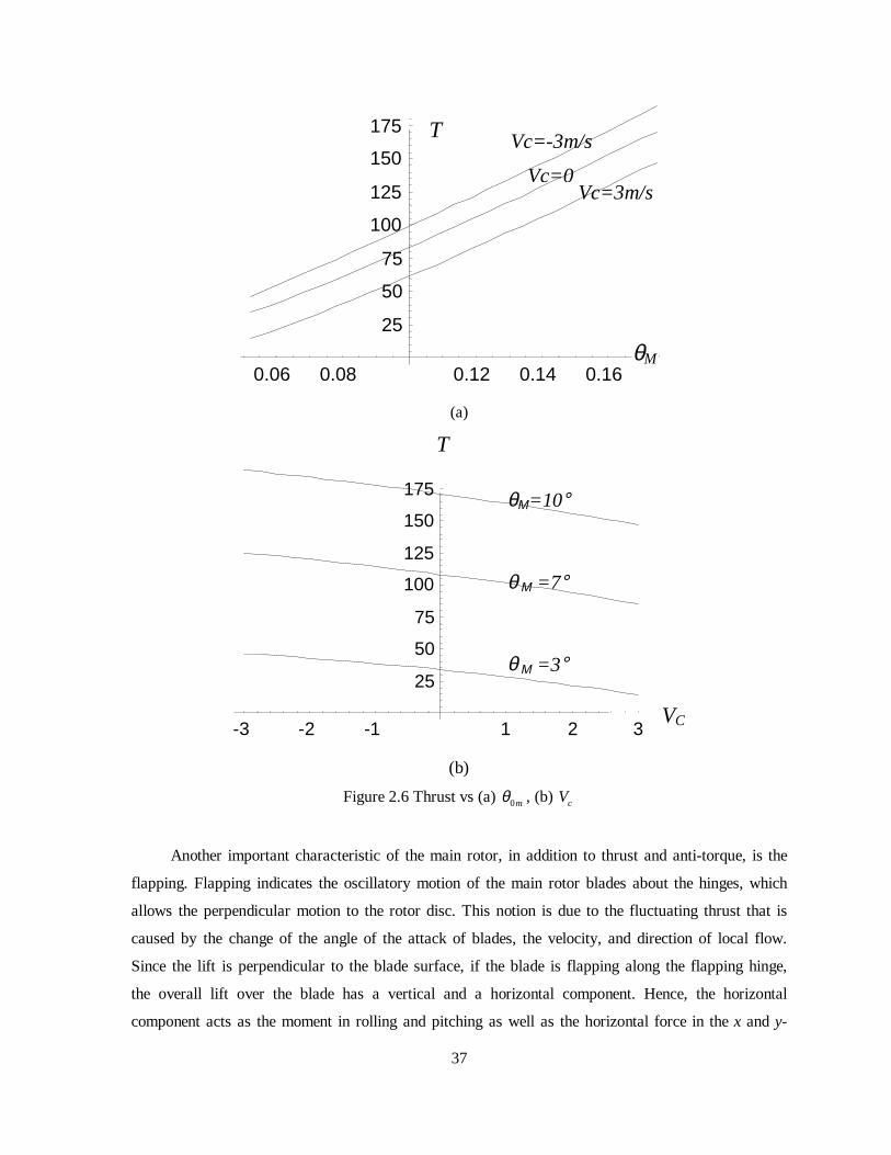
37

0.06 0.08 0.12 0.14 0.16 θM

25

50

75

100

125

150

175 T

Vc=0 Vc=3m/s

Vc=-3m/s

(a)

θ Μ =7°

-3 -2 -1 1 2 3 VC

25

50

75

100

125

150

175

T

θΜ=10°

θ Μ =3°

(b)

Figure 2.6 Thrust vs (a) 0mθ , (b) cV

Another important characteristic of the main rotor, in addition to thrust and anti-torque, is the

flapping. Flapping indicates the oscill atory motion of the main rotor blades about the hinges, which

allows the perpendicular motion to the rotor disc. This notion is due to the fluctuating thrust that is

caused by the change of the angle of the attack of blades, the velocity, and direction of local flow.

Since the lift is perpendicular to the blade surface, if the blade is flapping along the flapping hinge,

the overall li ft over the blade has a vertical and a horizontal component. Hence, the horizontal

component acts as the moment in rolli ng and pitching as well as the horizontal force in the x and y-

38

axis. The original concept of flapping was devised by an aerodynamicist Juan de la Cierva, who

conducted extensive study on autogiro. After experiencing mysterious rollover of his test autogiro, he

discovered that the unbalanced lift on the rotor disc was due to the increased forward velocity of the

vehicle. He thought that the unbalance could be alleviated by installi ng hinges for the blade grips to

allow blades to climb up and down by the amount of generated lift. Since helicopters have the same

problem with the unbalanced lift when they attain forward velocity, flapping is an important feature

in all helicopters. In addition to the flapping caused by the forward flight, flapping is also induced by

the mechanism called cyclic pitch. Cyclic pitch forces the blade to have a certain pitch angle which is

a function of azimuth, i.e., the rotation angle of the main rotor with respect to the fuselage. Cyclic

pitch is created by tilting the swashplate. The pitch lever attached to the blade follows the tilt angle of

the swashplate and forces the blade to have the cyclic pitch angle. In a full-size helicopter, the blade

pitch angle follows 90 in advance of the swashplate angle in order to compensate for the 90 phase

delay of gyroscopic effect. In other words, when the blade rotates and receives upward force due to

the increased lift by flapping, the blade starts tilting upward and reaches the maximum angle

approximately after one-quarter turn of the blade. Therefore, the longitudinal swashplate tilt induces

the pitch angle of the blade while the blade is still over the side. The maximum flapping is achieved

when the blade reaches the longitudinal position.

The cyclic pitch is produced by the ingenious linkage system and swashplate. The mechanism

of full-size helicopter is rather simple because the blade pitch level is directly connected to the

swashplate. The blade pitch can be written in terms of a Fourier series. While the blade pitch has

fixed geometric relationship with the swashplate, the flapping dynamics depend on the blade pitch,

the local flow, the helicopter body pitch and roll rate and so on. We will not go any further into the

flapping dynamics of full-size helicopters here because there are very different from that of small-size

helicopters1.

0 1 1 1cos sinr

A BR

θ θ θ= + − Ψ − Ψ (2.41)

where

θ : local blade pitch

1θ : blade twist(typically 0 in radio control helicopters)

1A : lateral cyclic pitch

1 Confusion arises due to the different direction of rotation of main rotor. Most civilian and military helicopters manufactured in the US has counterclockwise rotation viewed above. Most hobby helicopters and full-size helicopters manufactured outside of the US including those used in this research have clockwise rotation when viewed from above. The clockwise rotation is consistently assumed in the following including Figure 2.7 and Figure 2.8.

39

1B : longitudinal cyclic pitch

Ψ : azimuth angle

0Ψ = D

90Ψ = D

180Ψ = D

270Ψ = D

Figure 2.7 Swashplate and pitch level configuration

1A is positive when the pitch at 180Ψ = ° is larger. 1B is positive when the pitch on the

retreating blade is greater than the pitch on the advancing blade.

With the alternating blade pitch θ , the blade flaps up and down during its revolution with angle

β to the plane perpendicular to main rotor shaft. The angle β can be represented by Fourier series

and we can truncate the series by ignoring the higher order terms:

0 1 1 2 2

0 1 1

cos sin cos2 sin2

cos sins s s s

s s

a a b a b

a a b

β = − Ψ − Ψ − Ψ − Ψ− Ψ − Ψ

""

(2.42)

In the series (2.42), the constant term 0a is called coning, and only the first order coefficients

are used for flapping analysis. 1sa is called the longitudinal flapping with respect to a plane

perpendicular to the shaft defined as positive when the blade flaps down at the tail and up at the nose.

1sb is called the lateral flapping defined as positive when the blade flaps down on the advancing side

and up on the retreating side(Figure 2.8).

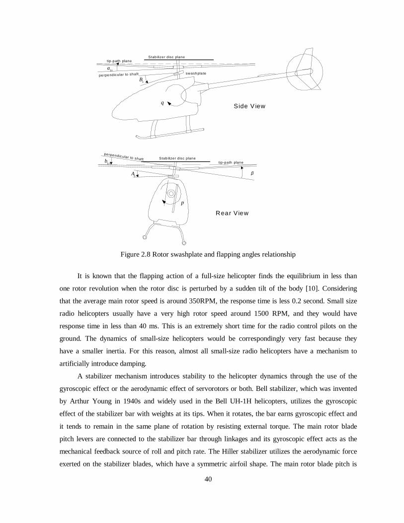
40

1saperpend icular to shaft

1sb

perpend icular to shaft

1A

1B

sw ashpla te

Side V iew

Rear View

β

p

q

Stab ilize r disc planetip -path plane

Stab ilize r disc planetip -path plane

Figure 2.8 Rotor swashplate and flapping angles relationship

It is known that the flapping action of a full-size helicopter finds the equili brium in less than

one rotor revolution when the rotor disc is perturbed by a sudden tilt of the body [10]. Considering

that the average main rotor speed is around 350RPM, the response time is less 0.2 second. Small size

radio helicopters usually have a very high rotor speed around 1500 RPM, and they would have

response time in less than 40 ms. This is an extremely short time for the radio control pilots on the

ground. The dynamics of small-size helicopters would be correspondingly very fast because they

have a smaller inertia. For this reason, almost all small-size radio helicopters have a mechanism to

artificially introduce damping.

A stabili zer mechanism introduces stabili ty to the helicopter dynamics through the use of the

gyroscopic effect or the aerodynamic effect of servorotors or both. Bell stabili zer, which was invented

by Arthur Young in 1940s and widely used in the Bell UH-1H helicopters, utili zes the gyroscopic

effect of the stabili zer bar with weights at its tips. When it rotates, the bar earns gyroscopic effect and

it tends to remain in the same plane of rotation by resisting external torque. The main rotor blade

pitch levers are connected to the stabili zer bar through linkages and its gyroscopic effect acts as the

mechanical feedback source of roll and pitch rate. The Hill er stabili zer utili zes the aerodynamic force

exerted on the stabili zer blades, which have a symmetric airfoil shape. The main rotor blade pitch is

41

controlled through the teetering motion of the stabili zer bar and the response of the blade is

aerodynamically damped. As the name implies, the Bell-Hill er stabili zer is a combination of two

distinct stabili zer mechanisms, i.e., the Bell-stabili zer and the Hill er stabili zer. This clever

combination of these two mechanisms has a stabili zer bar with stabili zer blades as well as the

weights. The role of Bell-Hill er stabili zer is also dual: the mechanical stabili zation by gyroscopic

effect of the tip weights and the mechanical servoing by the use of aerodynamic force on the stabili zer

blades.

This stabili zer mechanism consists of two paddle-shape blades attached to a rod hinged in its

middle on the tip of the main rotor shaft and other mixing linkages connecting from the swashplate to

the main rotor blade pitch control lever. In Figure 2.9, the Bell-Hill er stabili zer mechanism of the

Yamaha R-50 and the Kyosho Concept 60 are shown. The actual implementation of the stabili zer

mechanism differs slightly because the R-50 has a vertically moving swashplate and the Concept 60

has vertically fixed swashplate.

When the stabili zer bar rotates together with the main rotor blades, the stabili zer bar with

weights and blades develops gyroscopic action and aerodynamic force. The former reacts against any

external torque acting on the stabili zer disc and it retains the current attitude of rolli ng and pitching

for substantial time. The motion of the stabili zer bar is connected to the main rotor pitch levers

through a series of linkages.

The blades receive aerodynamic force proportional to their pitch angle. This aerodynamic force

exerts the teetering moment of the bar. The teetering motion is converted to the change of the main

rotor pitch. Due to the configuration of the blade pitch axis and the point where lift exerts on the

blade, the blade pitch has a restoring moment, which in turn acts to restore the teetering motion to

rest. These two moments seek the equili brium between the teetering motion and the restoring torque

of the rotor blades at significantly slower rate than the time constant of the rotor system without the

stabili zer mechanism. Therefore, the servomotors that actuate the swashplate do not have to supply a

large amount of force to overcome the restoring torque of the main rotor blades as the servomotors in

the full-size helicopters have to do. This unique approach of the use of aerodynamic force on the

stabili zer blades as the blade actuation force earned the name servorotor.

The teetering motion is a damped oscill atory motion, whose characteristic is determined by the

aerodynamic properties of the stabili zer blades and the main rotor blades. The amount of teetering is

determined by the rotor speed and the pitch angle of the stabili zer blades and it is the same as the tilt

angle of the swashplate.

42

(a) Yamaha R-50

(b) Kyosho Concept 60

Figure 2.9 Bell-Hill er Stabili zer system

The stabili zer dynamics can be modeled in a second order differential equation involving the

stabili zer bar and the rotor blade inertia, the aerodynamic force on the stabili zer blades and the rotor

blades and the mechanical feedback term from the gyroscopic effect of the stabili zer bar. Mettler [7]

proposed first-order model that characterizes the behavior of the Bell-Hill er stabili zer as shown in

(2.43).

Stabilizer blade

Stabilizer bar

43

1 1 1 1 1

1 1 1 1 1

11 1

11 1

s a s s b s s

s a s s b s s

ss b s u a u b

f

ss a s u a u b

f

aa q A b A u A u

bb p B a B u B u

τ

τ

= − − + + +

= − − + + +

(2.43)

Equation (2.43) is a first-order model of the flapping rotor dynamics, which accounts for the

coupled servorotor dynamics and mechanical feedback by the gyroscopic effect of the stabili zer bar.

fτ is the time constant of the servorotor response to the swashplate tilt angles. The body rate p and q

appear as feedback terms due to the gyroscopic effect of the stabili zer bar of the servorotor system.

The equations also include the input coupling terms, which are not small as shown later. The angular

rate dynamics are coupled with blade flapping angles ( 1sa , 1sb ) and body velocities (u, v). u and v

mainly are affected by the tilt angle pitch and roll, respectively and also by the flapping angles.

Research [7] shows this time constant fτ introduced by the use of the Bell-Hill er stabili zer is

approximately equal to five revolutions of the main rotor. For the Kyosho Concept 60 helicopter, fτ

is about 5/(1500RPM /60) 0.2= second. For the Yamaha R-50, 5/(900RPM /60) 0.333fτ = = .

As the closing remarks, it should be noted that the stabili zer bar does not stabilize the overall

vehicle dynamics. It merely introduces further damping to slow down the response so that the ground-

based pilot can control the vehicle with greater ease. Another observation is that the stabili zer

mechanism is not used for full-size helicopters any more because the stabili zer mechanism sacrifices

maneuverabili ty for the additional stabili ty. The dynamic characteristics of the vehicle can be

significantly improved by the use of electronic stabili ty and control augmentation system (SCAS) in

more versatile manner.

2.2.3 Tail Rotor

The primary role of tail rotor is to generate horizontal thrust varying by the collective pitch of

the tail rotor blades. With the moment arm provided by the tail boom, the tail rotor provides yawing

moment to counteract the anti-torque of the main rotor. It also produces the unbalanced horizontal

force, which acts as a drifting force in the y-direction. In hover, the helicopter tilts slightly in roll so

that the horizontal component of the main rotor thrust in the y-direction counteracts to the tail rotor

force.

44

The tail rotor consists of two or more symmetrically placed blades, a shaft and pitch control

mechanism. The configuration is simpler than the main rotor because they do not have cyclic pitch

control mechanisms, or stabili zer bars. Although small-size helicopters usually do not have flapping

hinges, the blades do undergo elastic deflection by the fluctuating aerodynamic force. In simplified

analysis, the tail rotor contributes to the yaw moment, sideslip and rolli ng moment depending on the

location of center of mass. The thrust and torque can be computed with equations (2.35) and (2.39)

with different values for tail rotor. The thrust dynamics with the sideslip or yaw is similar to the main

rotor dynamics in vertical motion, and hence it shows inherent stabili ty. However, when the

helicopter has significant cruise speed, the downwash from the main rotor as well as the inflow

affects the tail rotor and the horizontal stabili zer fin and resulting dynamics can be quite complicated.

2.2.4 Stabilizer Fins

The Horizontal and vertical stabili zer fins, which are attached to the tail boom, exert the

restoring moments in the pitching and the yawing directions, respectively when the vehicle has

forward velocity or head wind blows. Their role is similar to the role of their counterpart of fixed-

wing aircraft: to provide mechanical stabili zation when the vehicle has sufficient forward velocity or

it is exposed to headwind. The contribution of the fins appears as the forces and moments caused by

the aerodynamic lift and drag that are generated when the incoming airflow passes through these

components. The airflow around the fins becomes very complicated when the effect of inflow and the

downwash of the main rotor interact in high-speed cruise. In low velocity cruise or hover, they do not

have significant role and hence we can ignore the effect of the fins in the subsequent modeling.

While the fins of fixed-wing aircrafts always offer positive stabili zing effects, the fins in

helicopters may cause adversary effects when the helicopter experiences tail wind or side wind during

low-speed flight or hover. For example, when the tail wind blows a helicopter in hover, the vertical

stabili zer fin forces the yawing to deviate further. The horizontal fin shows similar effects in pitching

motion. Therefore, similar to airplanes, it is safe for helicopters to take off with head wind. In hover,

when there is no wind, the fins do not contribute to the helicopter in any significant way except to

create the vertical drag of the horizontal fin due to the main rotor downwash. In some designs

including the Yamaha industrial helicopters used for our research, the stabili zer fins are omitted or

miniaturized if the helicopter is not intended to fly at high speed.

45

Figure 2.10 Stabili zer fins of R-50 (left) and Concept 60 (right)

2.2.5 Fuselage

The fuselage receives drag and lift forces in all direction. The downward drag is produced by

blocking the inner part of the downwash of the main rotor. The horizontal li ft and drag are produced

when the helicopter gains speed or it is exposed to the wind. Definitely, the drag and the lift of the

fuselage are the function of the geometric shape. The horizontal drag of the fuselage is one of the

major factors for engine output and the maximum cruise speed. The vertical drag by the partial

blockage of the downwash acts as a parasite load. One interesting observation is that the helicopter

hovers with lesser power in the inverted flight, i.e., the helicopter flies upside down with the strong

negative pitch of the main rotor. In this state, the downwash of the main rotor is not blocked by the

body anymore and slight decrease of the power requirement for hover is observed. This has been

never attempted by the full-size helicopters, but it is one of the popular stunt flights by the advanced

hobby radio-controlled helicopter fliers.

The behavior of the drag and lift of the fuselage can be measured by the use of a wind tunnel or

estimated by the projected blocking area of the fuselage. However, similar to the stabili zer fins, the

horizontal and the vertical drag do not have the significant effect on the vehicle dynamics especially

when the helicopter is in hover. Therefore, it is also ignored in the simulation modeling in our study.

46

2.2.6 External Factors

The helicopter dynamics undergoes a transition when it takes off f rom the ground or lands back

on the earth. The ground exerts supporting force when all or some part of the landing gear touches the

ground. With a certain assumption, the ground support can be modeled into the simulation. Another

important factor is the ground effect, which indicates the phenomenon that less power is required to

generate a certain amount of lift when the helicopter is closer to the ground than the power required

for same amount of lift far from the ground [10,39]. The source of the ground effect is the decreased

magnitude of the induced velocity at the blade element, due to the blockage of the downwash by the

ground. The ground effect usually lasts up to the altitude of roughly the length of the main rotor

diameter. When the helicopter is very close to the ground, the ground effect can boost the thrust up to

100% more than the nominal thrust out of the ground effect region. Indeed, this is the underlying

theory of hovercraft, which floats only few inches over the ground by blowing air down. Ursa Minor

1, the first test RUAV for the Berkeley UAV research, could hover only in the ground effect region

because the engine could not keep up with the required load for ground effect-free flight.

Obviously, the ground effect is a very complicated and strongly nonlinear dynamic effect,

which is very hard to model analytically. From the viewpoint of controller design, the rotor efficiency

boost under the ground effect appears as larger control input gain. In the ground effect region, the

helicopter drifts more or feels like it is “riding on air” due to the unsteady wake of the main rotor

which is reflected on the ground. From these observations, the proposed controller should be robust to

the change of rotor efficiency as well as to the disturbance when the helicopter is in the ground effect.

The landing controller should be able to control the vertical descent following the landing profile

while minimizing the longitudinal and lateral drift to prevent tip-off of the helicopter.

2.2.7 Helicopter Hover Model

The Newton-Euler dynamic equations in (2.25) and (2.26) is valid throughout the entire flight

envelop as long as the accurate force and moment terms are found and used. It is often impossible to

find the force and moment terms that are accurate over the entire flight envelop. Therefore, we need

to limit the flight range to a certain flight mode to obtain more accurate and simpler equation form for

analysis. In our research, as has been implied so far, we start with hover mode because it is one of the

most important maneuvers of helicopter and low velocity horizontal/vertical motion and pirouette can

47

be considered as the extension of hover. In hover, the helicopter dynamics simplify in the following

ways:

• Since the vehicle has a very low velocity in every direction and the attitude deviation is small,

we can ignore the effect of the fuselage, the horizontal stabili zer and the vertical stabili zer.

( , ) 0

( , ) 0

( , , ) 0

F

H

V

X Y

X Y

X Y Z

===

(2.44)

• The tail rotor shaft is aligned along the +y axis and it does not generate any significant forces

by the local inflow in other direction. In other words, the tail rotor generates the lateral thrust,

and yaw moment and anti-torque in pitch axis only.

( , ) 0

( , ) 0T

T

X Z

R N

==

(2.45)

Under the assumption (2.44) and (2.45), the differential equation (2.25) simplifies to:

01

0M

b M T TP B

M H F

X vr wq

Y Y wp urm

Z Z Z g uq vp→

− = + + + − + + −

V R (2.46)

1 1

( )

( )

( )

M M M M M T T yy zz

b M M M M M T H H b zz xx

M M M T T xx yy

R Y h Z y Y h qr I I

M X h Z l M Z l pr I I

N Y l Y l pq I I

− −

+ + + − = − + + + + − − − −

& , , (2.47)

With the simplified system equation for hover, we find the aerodynamic equations for variables

in equation (2.47).

• Main rotor

The main rotor is the source of vertical li ft, horizontal force, and anti-torque. It also

generates the rolli ng and pitching moment by flapping, known as rotor stiffness, which is

produced by the vertical component of the blade centrifugal force acting at the hinge offset. The

overall contribution of the main rotor can be written as follows:

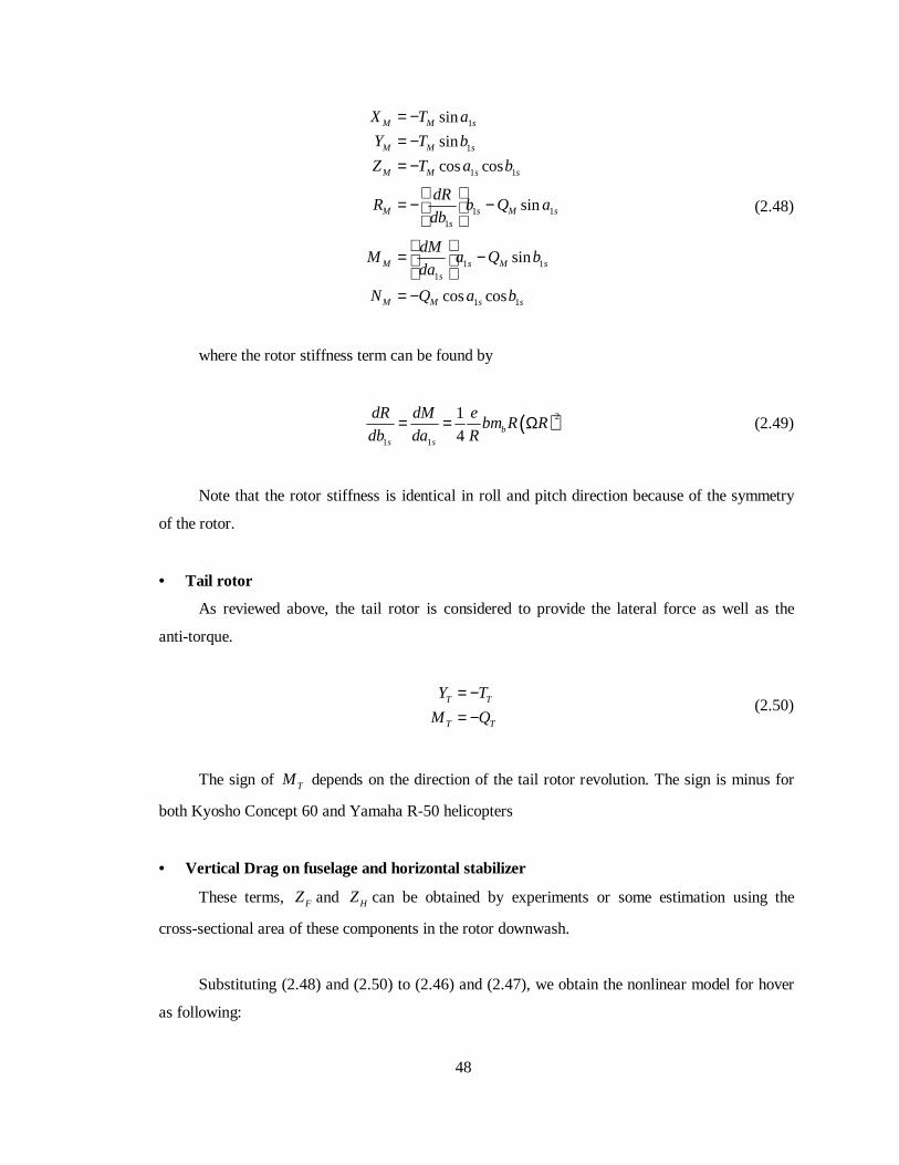
48

1

1

1 1

1 11

1 11

1 1

sin

sin

cos cos

sin

sin

cos cos

M M s

M M s

M M s s

M s M ss

M s M ss

M M s s

X T a

Y T b

Z T a b

dRR b Q a

db

dMM a Q b

da

N Q a b

= −= −= −

= − −

= −

= −

(2.48)

where the rotor stiffness term can be found by

( )2

1 1

1

4 b

s s

dR dM ebm R R

db da R= = Ω (2.49)

Note that the rotor stiffness is identical in roll and pitch direction because of the symmetry

of the rotor.

• Tail rotor

As reviewed above, the tail rotor is considered to provide the lateral force as well as the

anti-torque.

T T

T T

Y T

M Q

= −= −

(2.50)

The sign of TM depends on the direction of the tail rotor revolution. The sign is minus for

both Kyosho Concept 60 and Yamaha R-50 helicopters

• Vertical Drag on fuselage and horizontal stabili zer

These terms, FZ and HZ can be obtained by experiments or some estimation using the

cross-sectional area of these components in the rotor downwash.

Substituting (2.48) and (2.50) to (2.46) and (2.47), we obtain the nonlinear model for hover

as following:

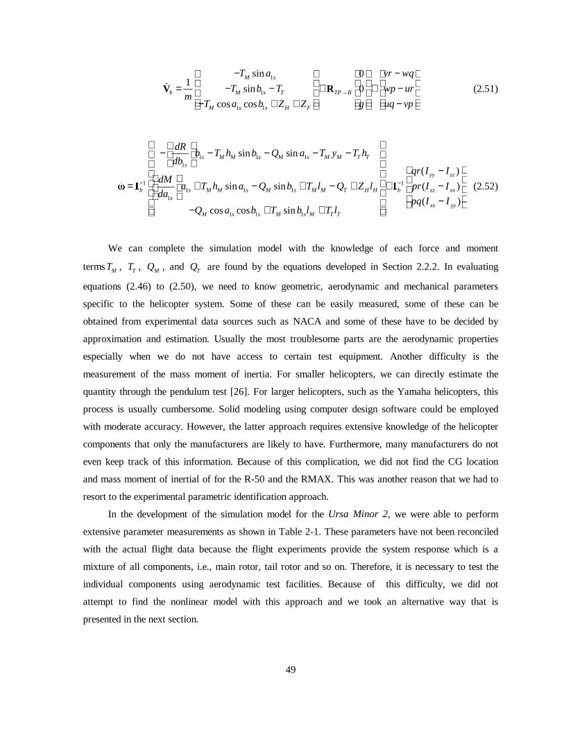
49

1

1

1 1

sin 01

sin 0

cos cos

M s

b M s T TP B

M s s H F

T a vr wq

T b T wp urm

T a b Z Z g uq vp→

− − = − − + + − − + + −

V R (2.51)

1 1 11

1 11 1 1

1

1 1 1

sin sin

( )

sin sin ( )

( )cos cos sin

s M M s M s M M T Ts

yy zz

b s M M s M s M M T H H b zz xxs

xx yy

M s s M s M T T

dRb T h b Q a T y T h

dbqr I I

dMa T h a Q b T l Q Z l pr I I

dapq I I

Q a b T b l T l

− −

− − − − −

− = + − + − + + − − − + +

& , ,

(2.52)

We can complete the simulation model with the knowledge of each force and moment

terms MT , TT , MQ , and TQ are found by the equations developed in Section 2.2.2. In evaluating

equations (2.46) to (2.50), we need to know geometric, aerodynamic and mechanical parameters

specific to the helicopter system. Some of these can be easily measured, some of these can be

obtained from experimental data sources such as NACA and some of these have to be decided by

approximation and estimation. Usually the most troublesome parts are the aerodynamic properties

especially when we do not have access to certain test equipment. Another difficulty is the

measurement of the mass moment of inertia. For smaller helicopters, we can directly estimate the

quantity through the pendulum test [26]. For larger helicopters, such as the Yamaha helicopters, this

process is usually cumbersome. Solid modeling using computer design software could be employed

with moderate accuracy. However, the latter approach requires extensive knowledge of the helicopter

components that only the manufacturers are likely to have. Furthermore, many manufacturers do not

even keep track of this information. Because of this complication, we did not find the CG location

and mass moment of inertial of for the R-50 and the RMAX. This was another reason that we had to

resort to the experimental parametric identification approach.

In the development of the simulation model for the Ursa Minor 2, we were able to perform

extensive parameter measurements as shown in Table 2-1. These parameters have not been reconciled

with the actual flight data because the flight experiments provide the system response which is a

mixture of all components, i.e., main rotor, tail rotor and so on. Therefore, it is necessary to test the

individual components using aerodynamic test facili ties. Because of this difficulty, we did not

attempt to find the nonlinear model with this approach and we took an alternative way that is

presented in the next section.

50

Se

rvom

oto

r/S

wa

shp

late

/M

ech

an

ical

Lin

kag

eS

yste

m

Ma

in R

oto

rT

hru

st D

yna

mic

s

Se

rvoro

tor

Dyn

am

ics

0M

uθ

0T

uθ

1 as

u

1 bs

u

0M

θ

0T

θT

ail R

oto

rT

hru

st D

yna

mic

s

1A

1B

Attitu

de

Dyn

am

ics

1s

a

1s

b

Ma

in R

oto

r Dyn

am

ics

Ya

w D

yn

am

icsT

T MT

Ve

rtical

Dyn

am

ics

Ho

rizo

nta

lV

elo

city

Dyn

am

ics

wr

uvE

ule

rA

ng

le

Eu

ler

An

gle

Inte

gra

tion

ΦΘ

pq

wpqrΨ

TP

xV

TP

yV

TP

zV

Inte

gra

tion

TP

xP

TP

yP

TP

zP

uv

Se

rvom

oto

r/M

ech

an

ical

Lin

kag

e

Figure 2.11 Block diagram representation of helicopter dynamics

51

The vehicle model developed so far can be implemented in a simulation environment. In

choosing the simulation environment, there are a number of choices available. MATLAB is one of the

most popular design and simulation environments because it offers abundant numerical algorithms

and design tools as well as nice visualization functions. For the simulation, MATLAB offers

graphical user interface-based numerical simulation environment, Simulink®. In this research,

MATLAB/Simuli nk is consistently used for controller design and simulation. In the Simulink

environment, the helicopter dynamics developed so far is cast into Simulink S-functions in the C

language, which is chosen for faster execution time.

The helicopter equations that have been formulated so far can be represented in the following

block diagram. It should be noted that, quite contrary to some understandings, the helicopter

dynamics are not a cascade of servomotor-attitude-translational sub-dynamics. The feedback of

angular rates p and q due to the Bell-Hill er stabili zer system modifies the dynamics substantially. The

horizontal velocity u and v also affects the attitude dynamics. If the helicopter is constrained in the

translational motion and only the attitude motion is allowed, the attitude dynamics is stable. However,

when it is allowed to move freely in the horizontal direction, the vehicle dynamics becomes unstable

due to the interaction of the lift and the inflow.

As can be seen in the block diagram, the helicopter system has four inputs while the helicopter

has the freedom in 3 SO(3)×5 . Therefore, the helicopter is an underactuated system, which implies

that the vehicle dynamics has internal constraints so that only four DOF can be arbitrarily achieved

while the other two are constrained by the configuration of the helicopter. The helicopter achieves the

longitudinal motion and the lateral motion by tilting the body first in pitch and roll direction,

respectively. The attained velocity in x and y direction has certain relationship with the amount of the

angle tilted in pitch and roll direction, respectively. In normal situation, this would not pose any

significant restriction in navigation. The peculiar situation occurs during the landing: due to the

dynamic relationship between the attitude and the translational velocities in the x and y direction, the

helicopter has difficulties to land on a slanted surface. This has been known to be a problem when a

helicopter attempts to land on a rolli ng and pitching deck of a ship.

• Linearized Model

The nonlinear model (2.46) for hover is valuable for the nonlinear simulation model and it can

be further simplified to obtain the linear model. A linear dynamic model for helicopter is needed for

the design of linear feedback control system. As shown in Figure 2.11, the helicopter dynamics can be

decomposed into three parts: (1) servoactuator-mechanical li nkage system, (2) aerodynamics system,

and (3) kinematic system. In the previous sections, the kinematic-dynamic relationship for (2) and (3)

52

are developed. The subsystem (1) is relatively easier to identify and the response time is usually faster

than that of the aerodynamic systems. Therefore, in the subsequent analysis, the servoactuation

dynamics is embedded in the much slower-to-respond consequential dynamics and will be identified

together. With this consideration, we define the following nonlinear helicopter dynamics

( , )=x F x u (2.53)

where

1 1[ ]Ts su v w p q r a b= Φ Θ Ψx (2.54)

1 1

[ ]s s M T

Ta bu u u uθ θ=u (2.55)

1sau : input to the lateral cyclic pitch

1sbu : input to the longitudinal cyclic pitch

M

uθ : input to the main rotor collective pitch

T

uθ : input to main rotor collective pitch

For the nonlinear control model, we can directly use the nonlinear simulation model or a model

with simplifications and/or approximations of the thrust and torque terms. In this research, we are

interested in finding the linear time invariant model for LTI identification and controller design for

hover. Therefore, we introduce the following assumptions:

• The velocity and attitude angles are assumed to be very small so that the following

simplifications are valid:

sin , cos 1x x x (2.56)

• With the assumption that the rigid body has small velocity and attitude angles in every

direction, the Coriolis’ acceleration terms and gyroscopic terms are ignored.

0 0 0

0 0 0yy zz xx yyzz xx

xx yy zz

yr zq xr zp xq yp

I I I II Iqr pr pq

I I I

− − + −− −−

(2.57)

Applying (2.56) and (2.57) to the original equation, we obtain the differential equation

53

( )

( )

( )

1

1

1 11

1 11

1

1

( , )

1

1

1

1

1

1

M s

M s T

M H F

M M s M s M M T Txx s

M M s M s M M T H Hyy s

M M s M T Tzz

s

f

T a gm

T b T gm

T Z Z gm

p

dRT h b Q a T y T h

I db

q

dMT h a Q b T l Q Z l

I da

r

Q T b l T lI

aq

τ

=

− − Θ

− + + Φ

− + + +

− + − − −

= + − + − +

− + +

− − +

x F x u

1 1 1 1 1

1 1 1 1 1

1

11

s a s s b s s

s a s s b s s

b s u a u b

sa s u a u b

f

A b A u A u

bp B a B u B u

τ

+ + − − + + +

(2.58)

Note that the force and moment terms are the function of a number of parameters as following:

: ( , , , )

:

: ( , , )

:

M

M

T

T

T M M

Q M M

T T T

Q T T

f u v w T

f Q

f v r T

f Q

θθ

θ

θ

6

6

6

6

(2.59)

The linearized system equation is defined as the Jacobian matrices in the following:

trim trim

trim trim

j j

i i

F F

x uδ δ δ

= == =

∂ ∂ = + ∂ ∂ x x x x

u u u u

x x u (2.60)

where

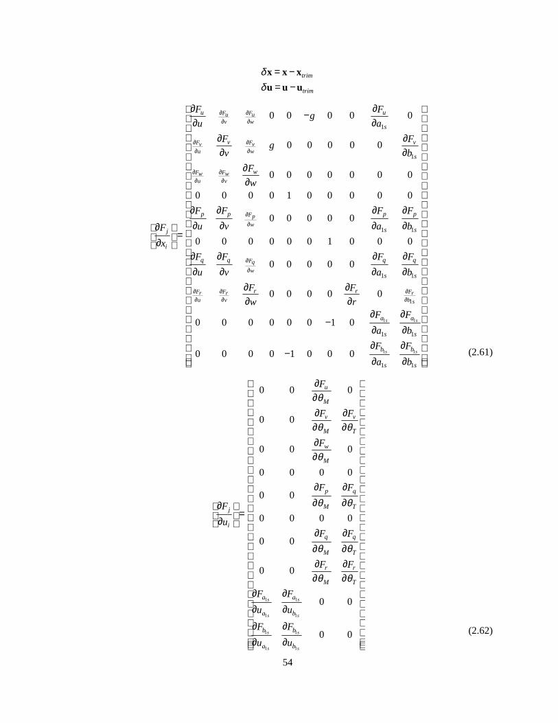
54

trim

trim

δδ

= −= −

x x x

u u u

1

1

1 1

1 1

0 0 0 0 0

0 0 0 0 0

0 0 0 0 0 0 0

0 0 0 0 1 0 0 0 0 0

0 0 0 0 0

0 0 0 0 0 0 1 0 0 0

0 0 0 0 0

0 0 0 0

F Fu uv w

F Fv vu w

F Fw wu v

Fp

w

Fq

w

F Fr ru v

u u

s

v v

s

w

p p p p

s sj

i

q q q q

s s

r

F Fg

u a

F Fg

v b

F

w

F F F F

u v a bF

xF F F F

u v a b

F

w

∂ ∂∂ ∂

∂ ∂∂ ∂

∂ ∂∂ ∂

∂

∂

∂

∂

∂ ∂∂ ∂

∂ ∂−

∂ ∂∂ ∂∂ ∂

∂∂

∂ ∂ ∂ ∂∂ ∂ ∂ ∂∂

= ∂ ∂ ∂ ∂ ∂∂ ∂ ∂ ∂

∂ ∂∂

1 1

1 1

1

1 1

1 1

0

0 0 0 0 0 0 1 0

0 0 0 0 1 0 0 0

s s

s s

Frb s

r

a a

s s

b b

s s

F

rF F

a b

F F

a b

∂∂

∂ ∂ ∂ − ∂ ∂

∂ ∂ − ∂ ∂ (2.61)

1 1

1 1

1 1

1 1

0 0 0

0 0

0 0 0

0 0 0 0

0 0

0 0 0 0

0 0

0 0

0 0

0 0

s s

s s

s s

s s

u

M

v v

M T

w

M

p q

M Tj

i

q q

M T

r r

M T

a a

a b

b b

a b

F

F F

F

F F

F

uF F

F F

F F

u u

F F

u u

θ

θ θ

θ

θ θ

θ θ

θ θ

∂ ∂ ∂ ∂ ∂ ∂ ∂ ∂

∂ ∂ ∂ ∂∂ = ∂ ∂ ∂ ∂ ∂

∂ ∂ ∂ ∂

∂ ∂ ∂ ∂ ∂ ∂ ∂ ∂

(2.62)

55

The Jacobian, often referred to as the stability derivatives in the aerospace community, can be

found by the partial differentiation of the system equation F(x,u) as shown in (2.61) and (2.62). The

terms with negligible contributions are displayed with smaller fonts. The valuable results on

calculating the Jacobian were suggested by Prouty [10]. Using his work, the Jacobian matrices can be

computed by simply plugging in the parameters of the target helicopter as shown in Table 2-1. Most

of his work is directly applicable to our research with the exception of the flapping characteristics.

The Jacobian in (2.61) and (2.62) provides us the insights on the relationship between the contribution

of each term and the overall vehicle dynamics. This analysis is particularly useful for the vehicle

design and tuning process to meet the handling quality requirements.

In Table 2-1, the various parameters of Ursa Minor 2 are listed. The meanings of these

parameters are mostly self-explanatory. The inertia terms are measured by a simple pendulum test.

The geometric terms are determined easily once the location of C.G. is found. The airfoil of the main

rotor of the Ursa Minor 2 is assumed NACA0012 and its aerodynamic parameters are determined by

the experiments by NACA in 1950s. The airfoil of the tail rotor is close to NACA0014 and the

aerodynamic parameters are determined in a similar way. The operational parameters such as the

angular velocity of main rotor and the hover pitch are found by a series of test flights.

As mentioned earlier, we have difficulty directly pursuing this approach because, in the case of

Yamaha R-50 for example, most of the aerodynamic and mechanical parameters are difficult to find.

R-50 is too large and heavy to measure the inertia directly. The aerodynamic property of the custom-

shape blades of R-50 is difficult to estimate without any test facili ty. Therefore, we seek an

alternative way to find a system model directly using the flight data.

56

Table 2-1 Parameters for Ursa Minor 2 for simulation model Rotor CW

Rho 1.18 c

Vertical Drag/mg H 0

Vertical Drag/mg F 0.02

Weight 93.12 9.5

Ixx 0.1634 c

Iyy 0.5782 c

Izz 0.6306 c

Mass of main blade 0.178 c

Ibm 0.0280 c ******

Qm 2.5110 c

Angular Vel. of M.Rotor 171.1 1634.32 RPM MACH Number 0.39766199144

Radius of M.Rotor 0.79 c

Inner radius of M.Rotor 0.196 c

Pitch angle at root 0.1257 7.2 deg

Twist of Main blade 0 c Normalization Numbers a0 0.04674 c

Sigma of M.Rotor 0.04980 c Max.Vx 5 m/s

Pitch angle at 75% 0.1257 c Max.Vy 5 m/s

Flapping offset ratio (e/R) 0.05063 c Max.Vz 5 m/s

Slope of lift curve of M.Rotor 5.40 s Max.Roll_angle 0.3491 rad

Drag coefficient Cd of M.Rotor 0.006400 s Max.Roll_rate 0.3491rad/s

# of M.blade 2 c Max.Pitch_angle 0.3491rad

width of M.Rotor 0.058 c Max.Pitch_rate 0.3491rad/s

Area of M.blade 0.0916 c Max.Yaw_angle 0.3491rad

iM -0.03491 c Max.Yaw_rate 0.3491rad/s

hM 0.2340 c Max.Collective_pitch 0.0873rad

yM 0 c Max.Tail_pitch 0.4363rad

lM 0.01 c Max.Lateral_cyclic_pitch 0.3491rad

lF -0.1 c Max.Longitudinal_cyclic_pitch 0.4363rad

lH 0.00 N/A Servo_Corner_Frequency 6.2832Hz

Angular Vel. of T.Rotor 920.8 8792.646 RPM Servo_Gain 66.82

Radius of T.Rotor 0.1290 c Max.Servo_Pulse_width 800

Inner radius of T.Rotor 0.042 c

Slope of lift curve of T.Rotor 5.40 s MACH Number 0.34934857633

Drag coefficient Cd of T.Rotor 0.006400 s

Sigma of T.Rotor 0.1198 c

#.of Blade T.Rotor 2 c Linkage Gain

width of T.Rotor 0.028 c Main 1.9248

Area of Blade T.Rotor 0.0056 c Tail 2.3955

F to T ratio 0.053 s Lingitudinal 1.9289

Thrust of T.Rotor 5.553 c Lateral 1.5431

V1t 7.095 c

Torque of T.Rotor 0.02965 c

Pitch angle at 75% T.Rotor 0.1414 8.1 0

ht 0.0620 c

lt 0.8980 c

Gear Ratio (Main Rotor/Engine) 9.79

Gear Ratio (Tail Rotor/Engine) 5.38

Angular Vel. of Engine 1675.5 16000

57

2.2.8 Experimental Hover Model

In the previous sections, a general nonlinear system model for hover has been developed. This

model is very useful for the construction of simulation model if and only if the accurate knowledge

over numerous system parameters and rotor force and moment models is available. In our research,

we estimated the full set of parameters for Ursa Minor 2 as shown in Table 2-1. As mentioned above,

the estimated parameters were not reconciled with the flight data and the obtained nonlinear model

may not correctly describe the actual helicopter dynamics. The major difficulty of this approach is

that the accurate knowledge of the aerodynamic parameters as well as some other mechanical

parameters are hard to obtain and the reconcili ation of the theoretical model with the experimental

data is impossible without proper experimental setup. In our research, this situation forced us to resort

to the empirical parametric identification method instead of the theoretical model approach. The

parameters that have to be identified are the Jacobians in the linearized model. While the parameters

of the nonlinear model developed above are physical mechanical or aerodynamic parameters, the

parameters in the Jacobian are the first-order derivative of the complicated nonlinear functions in

(2.58). As we decided to identify the helicopter model as is, a number of changes are made to the

original nonlinear or linear models proposed in Section 2.2.7. In the following, the template model for

the LTI MIMO parametric identification is given. This model is proposed by Mettler et al in 1999: it

is a simplified version of (2.61) and (2.62) obtained by discarding terms of negligible contributions.

This model also includes the servorotor dynamics as a first-order approximation. The servomotor

models for the control surfaces are embedded in the system matrices and identified together because

the bandwidths of the servomotors are sufficiently higher than the retarded response speed of the

servorotor and lift dynamics of main and tail rotors. Another major modification is the inclusion of

the built-in rate gyroscope compensator model. As will be explained in a greater detail i n Section 3.1,

the rate gyroscope senses the yaw rate and superpose the yaw compensation signal on the pilot’s

command. The feedback system attenuates the effect of the anti-torque fluctuation on the yaw

response so that the ground pilot to control the vehicle with ease. It was decided to leave the built-in

gyroscope in the loop because of the two reasons: (1) the yaw response can be improved without

additional yaw rate feedback if tuned correctly, and (2) it helps the human pilot to take over the

control of the vehicle in emergency.

With these factors, the template model has the input to the servomotor as the control input

variables. In the yaw channel, the input is no longer the tail collective pitch: it is now the input to the

yaw rate compensator. By having the servomotor PWM input as the control input, we do not need to

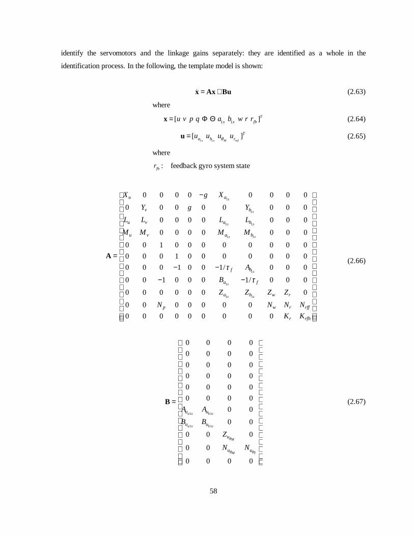
58

identify the servomotors and the linkage gains separately: they are identified as a whole in the

identification process. In the following, the template model is shown:

= +x Ax Bu (2.63)

where

1 1[ ]Ts s fbu v p q a b w r r= Φ Θx (2.64)

1 1

[ ]s s M ref

Ta b ru u u uθ=u (2.65)

where

fbr : feedback gyro system state

1

1

1 1

1 1

1

1

1 1

0 0 0 0 0 0 0 0

0 0 0 0 0 0 0 0

0 0 0 0 0 0 0

0 0 0 0 0 0 0

0 0 1 0 0 0 0 0 0 0 0

0 0 0 1 0 0 0 0 0 0 0

0 0 0 1 0 0 1/ 0 0 0

0 0 1 0 0 0 1/ 0 0 0

0 0 0 0 0 0 0

0 0 0 0 0 0 0

0 0 0 0 0 0 0 0 0

s

s

s s

s s

s

s

s s

u a

v b

u v a b

u v a b

f b

a f

a b w r

p w r rff

r rfb

X g X

Y g Y

L L L L

M M M M

A

B

Z Z Z Z

N N N N

K K

τ

τ

−= − −

− −

A

(2.66)

1 1

1 1

0 0 0 0

0 0 0 0

0 0 0 0

0 0 0 0

0 0 0 0

0 0 0 0

0 0

0 0

0 0 0

0 0

0 0 0 0

a s b s

a s b s

M

M T

u u

u u

u

u u

A A

B B

Z

N Nθ

θ θ

=

B (2.67)

59

A MIMO model can be identified with a number of numerical optimization algorithms. In our

research, a time-domain based optimization tool is used as will be explained in detail.

To identify the parameters in the system matrices (2.66) and (2.67), we need to collect flight

data first. The UAV platforms are equipped, as will be explained in detail i n next chapter, with

hardware and software that measure the pilot’s control input and the vehicle response. During the test

flight, the pilot issues frequency-sweeping control input in each channel, namely roll, pitch, yaw, and

vertical and the vehicle response was recorded. Although the task sounds straightforward, the actual

experiment is more involved and risky due to the unstable helicopter response, the complication of

platform/hardware/software reliabili ty, and the perturbed vehicle response due to many factors such

as wind and temperature.

In a certain interval, longitudinal and lateral controls are issued in mixed way to capture the

cross-coupling of these two channels. One flight data is shown in Figure 2.12: in the first stage, the

controls in the longitudinal and the lateral channels are given simultaneously in order to capture the

coupling between these axes, while other channels are controlled to maintain constant altitude and

heading. In the latter two stages, the main rotor collective pitch or the tail collective pitch are

perturbed. Finally, the control signal is issued into all channels simultaneously to check the validity of

the cross-coupling term. It should be noted that, due to the coupled and unstable dynamics, the pilot

has to issue a stabili zing command to keep the helicopter in a confined area. This hinders the data

collection of a one-channel-at-a-time response.

Once adequate flight data has been collected, we identify the parameters in the system matrices

using an identification algorithm. Before feeding the data into the numerical tool, the data is

preprocessed. The angular rate measurements are filtered by zero-phase non-causal discrete-time

filters to filter out high frequency noise without introducing phase delay. The roll and pitch angle

measurements are detrended because the helicopter has a trim condition, i.e., the equili brium with

certain nonzero states. In this research, the prediction-error method (PEM) in the MATLAB System

Identification Toolbox is chosen.

• Prediction-error method [34]

Suppose we consider a discrete-time state space model

( 1) ( ) ( ) ( )

( ) ( ) ( ) ( )

x k Ax k Bu k Ke k

y k Cx k Du k e k

+ = + +

= + + (2.68)

where

xnx∈5

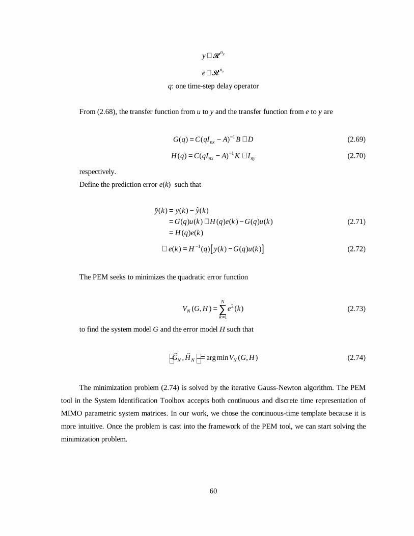
60

yny∈5

yne∈5

q: one time-step delay operator

From (2.68), the transfer function from u to y and the transfer function from e to y are

1( ) ( )nxG q C qI A B D−= − + (2.69)

1( ) ( )nx nyH q C qI A K I−= − + (2.70)

respectively.

Define the prediction error e(k) such that

ˆ( ) ( ) ( )

( ) ( ) ( ) ( ) ( ) ( )

( ) ( )

y k y k y k

G q u k H q e k G q u k

H q e k

= −= + −=

(2.71)

[ ]1( ) ( ) ( ) ( ) ( )e k H q y k G q u k−∴ = − (2.72)

The PEM seeks to minimizes the quadratic error function

2

1

( , ) ( )N

Nk

V G H e k=

= ∑ (2.73)

to find the system model G and the error model H such that

ˆ ˆ, argmin ( , )N N NG H V G H = (2.74)

The minimization problem (2.74) is solved by the iterative Gauss-Newton algorithm. The PEM

tool in the System Identification Toolbox accepts both continuous and discrete time representation of

MIMO parametric system matrices. In our work, we chose the continuous-time template because it is

more intuitive. Once the problem is cast into the framework of the PEM tool, we can start solving the

minimization problem.

61

0 20 40 60−10

−5

0

Zup

[m/s

]

0 20 40 60−1

0

1V

up [m

/s]

0 20 40 60−250

−200

−150

Yaw

[deg

]

0 20 40 60−50

0

50

100

r [d

eg/s

]

0 20 40 601.4

1.6

1.8

2

u θ M

[deg

]

0 20 40 601.4

1.5

1.6

1.7

u θ T [d

eg]

0 20 40 60−2

−1

0

1

Vb x [m

/s]

0 20 40 60−1

0

1

2

Vb y [m

/s]

0 20 40 60−10

0

10

pitc

h [d

eg]

0 20 40 60−10

0

10

20

roll

[deg

]

0 20 40 60−100

0

100

p [d

eg/s

]

0 20 40 60−100

0

100

q [d

eg/s

]

0 20 40 601.5

1.6

1.7

1.8

u B1 [d

eg]

time [sec]0 20 40 60

1.4

1.6

1.8

u A1 [d

eg]

time [sec]

Figure 2.12 Sample flight data for system identification of Ursa Magna 2

It should be noted that this method is extremely sensitive to the initial guess of the parameters.

It is also easily trapped in local minima of the parameter hypersurface. To obtain meaningful results

and not some parameter set that blindly matches the time history while avoiding these weaknesses,

the following technique is devised. First, the angular dynamics, which are augmented with the rotor

dynamics, is identified using an initial guess. Since the angular rate/rotor dynamics are known to be

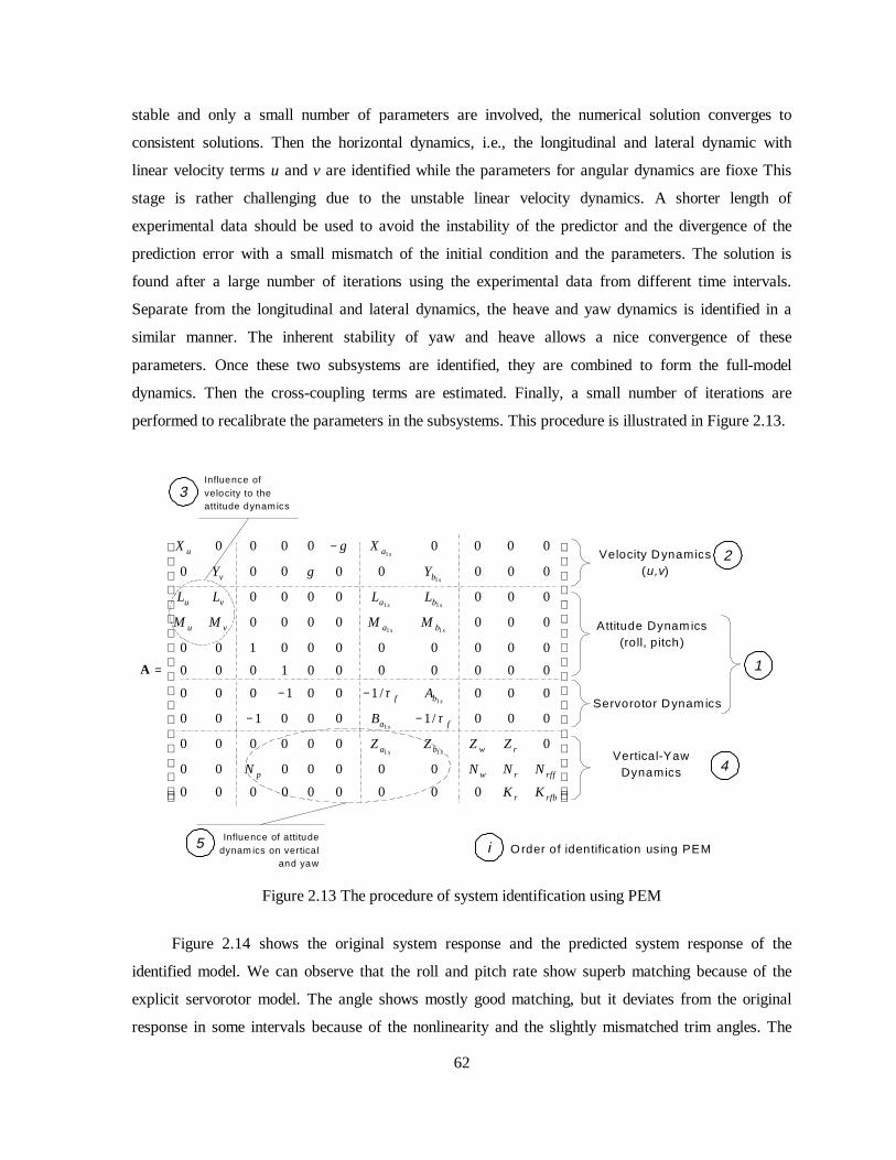
62

stable and only a small number of parameters are involved, the numerical solution converges to

consistent solutions. Then the horizontal dynamics, i.e., the longitudinal and lateral dynamic with

linear velocity terms u and v are identified while the parameters for angular dynamics are fioxe This

stage is rather challenging due to the unstable linear velocity dynamics. A shorter length of

experimental data should be used to avoid the instabili ty of the predictor and the divergence of the

prediction error with a small mismatch of the initial condition and the parameters. The solution is

found after a large number of iterations using the experimental data from different time intervals.

Separate from the longitudinal and lateral dynamics, the heave and yaw dynamics is identified in a

similar manner. The inherent stabili ty of yaw and heave allows a nice convergence of these

parameters. Once these two subsystems are identified, they are combined to form the full-model

dynamics. Then the cross-coupling terms are estimated. Finally, a small number of iterations are

performed to recalibrate the parameters in the subsystems. This procedure is ill ustrated in Figure 2.13.

1

1

1 1

1 1

1

1

1 1

0 0 0 0 0 0 0 0

0 0 0 0 0 0 0 0

0 0 0 0 0 0 0

0 0 0 0 0 0 0

0 0 1 0 0 0 0 0 0 0 0

0 0 0 1 0 0 0 0 0 0 0

0 0 0 1 0 0 1/ 0 0 0

0 0 1 0 0 0 1/ 0 0 0

0 0 0 0 0 0 0

0 0 0 0 0 0 0

0 0 0 0 0 0 0 0 0

s

s

s s

s s

s

s

s s

u a

v b

u v a b

u v a b

f b

a f

a b w r

p w r rf f

r rfb

X g X

Y g Y

L L L L

M M M M

A

B

Z Z Z Z

N N N N

K K

τ

τ

−

= − −

− −

A

Velocity Dynamics(u,v)

Attitude Dynam ics(roll, pitch)

Servorotor Dynam ics

Vertical-YawDynamics

Influence ofvelocity to theattitude dynamics

Influence of attitudedynam ics on vertica l

and yaw

1

2

4

3

5 i Order of identification using PEM

Figure 2.13 The procedure of system identification using PEM

Figure 2.14 shows the original system response and the predicted system response of the

identified model. We can observe that the roll and pitch rate show superb matching because of the

explicit servorotor model. The angle shows mostly good matching, but it deviates from the original

response in some intervals because of the nonlinearity and the slightly mismatched trim angles. The

63

vertical model shows rather poor matching in some intervals because the actual vertical dynamics is a

very complicated combination of the engine, the transient lift, and the cross-coupling with the roll,

pitch and yaw. A higher-order model may be used to account for the transient behavior of the lift

dynamics. In the following, the identified system matrices for Ursa Magna 2 are shown.

0.1257 0 0 0 0 0 0 0 0

0 0.4247 0 0 0 0 0 0 0

0.1677 0.0870 0 0 0 0 36.7050 161.1087 0 0 0

0.0823 0.0518 0 0 0 0 63.5763 19.4931 0 0 0

0 0 1 0 0 0 0 0 0 0 0

0 0 0 1 0 0 0 0 0 0 0

0 0 0 1 0 0 3.4436 0.8287 0 0 0

0 0 1 0 0 0 0.3611 3.4436 0 0 0

0 0 0 0 0 0 0 9.6401 0.7598 8.4

g g

g g

− − −−

−− − −

=− −

− −−

A

231 0

0 0 1.3300 0 0 0 0 0 0.0566 5.5105 44.8734

0 0 0 0 0 0 0 0 0 1.8157 11.0210

− − −

−

(2.75)

0 0 0 0

0 0 0 0

0 0 0 0

0 0 0 0

0 0 0 0

0 0 0 0

0.8417 2.8231 0 0

2.4090 0.3511 0 0

0 0 70.5041 0

0 0 23.6260 44.8734

0 0 0 0

= − − −

B (2.76)

Table 2-2 Eigenvalues of the identified helicopter system

Mode Value Damping Frequency (rad/s)

Phugoid 1 -0.52620.0755j 0.990 0.532

Phugoid 2 0.24580.0279j -0.994 0.247

Roll -1.572512.2567j 0.127 12.4

Pitch -1.86598.2757j 0.220 8.48

Yaw -8.28458.5845j 0.694 11.9

Heave -0.7223 1 0.722

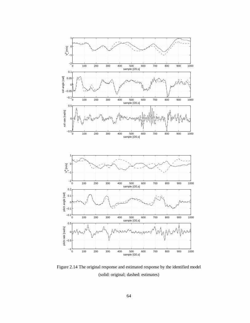
64

0 100 200 300 400 500 600 700 800 900 1000−2

−1

0

1

sample [/20,s]V

b x [m/s

]

0 100 200 300 400 500 600 700 800 900 1000−0.1

−0.05

0

0.05

0.1

sample [/20,s]

roll

angl

e [r

ad]

0 100 200 300 400 500 600 700 800 900 1000−0.5

0

0.5

sample [/20,s]

roll

rate

[rad

/s]

0 100 200 300 400 500 600 700 800 900 1000−2

−1

0

1

sample [/20,s]

Vb y [m

/s]

0 100 200 300 400 500 600 700 800 900 1000−0.2

−0.1

0

0.1

0.2

sample [/20,s]

pitc

h an

gle

[rad

]

0 100 200 300 400 500 600 700 800 900 1000−1

−0.5

0

0.5

sample [/20,s]

pitc

h ra

te [r

ad/s

]

Figure 2.14 The original response and estimated response by the identified model

(solid: original; dashed: estimates)

65

0 100 200 300 400 500 600 700 800 900 1000−0.8

−0.6

−0.4

−0.2

0

0.2

0.4

0.6

sample [/20,s]

Vb z [m

/s]

0 100 200 300 400 500 600 700 800 900 1000−0.6

−0.4

−0.2

0

0.2

0.4

0.6

0.8

sample [/20,s]

yaw

rat

e [r

ad/s

]

Figure 2.14 (‘cont)

The eigenvalues of the identified model are listed in Table 2-2.The linearized system model has

stable eigenvalues except for only one pair of complex conjugate in right half plane, which renders

the whole helicopter dynamics unstable. This unstable mode is the coupled motion in u and v

channels and it shows almost pure divergence because time constant is very large (25 seconds). The

responses in all other channels are stable. The roll and pitch responses are weakly damped and their

time constants are about 0.51 and 0.74 second, respectively. The rotor dynamics is essentially

symmetric and the difference between them is generated by the different values of the mass moment

of inertia in the roll and the pitch axis.

The yaw response is moderately damped and the response is fast. This well-tuned response is

due to the built-in yaw rate damping gyro system. The heave response shows pure convergence in the

first-order quasi-static model and the time constant is about 8.7 seconds. This is anticipated by the

experience in manual control of R-50.

66

Chapter 3

3. Hardware, Software, and Vehicle

Integration

One of the main goals of the Berkeley UAV research effort is to develop and establish a

comprehensive and practical methodology to design and implement multiple number of RUAVs

equipped with a reliable high-accuracy autopilot. To demonstrate this idea, we need to integrate the

vehicle platform with the proper hardware and software so that the vehicle can perform the desired

autonomous maneuvers. The integration process is not trivial in every detail because there are many

limits and unforeseen interactions when individual components are installed and connected together

mechanically and electronically. Indeed, an RUAV is a very tightly integrated embedded electro-

mechanical system: every onboard component has an impact on the mechanical aspects such as mass,

rotational inertia, and the center of gravity shift of the overall vehicle. In electronic aspects,

electromagnetic interference may be a problem for sensitive devices such as the GPS and the digital

compass. The small-size radio-controlled helicopters have very limited payload and mounting spaces,

and hence we do not have the luxury to apply high-grade protection materials and mountings in order

to isolate problems. In many cases, we are forced to provide minimal protection against vibration,

heat, and EMI.

The operation of the helicopter platform is hazardous. The high-speed rotor blades pose

significant potential threats on ground crew, any other people in the area, and buildings or any

properties nearby because the main and tail rotor blades rotate at very high speeds. Moreover, unlike

other experimental testbeds that are typically operated in isolated and stable indoor environments,

RUAVs operate in a hostile environment. Another demanding factor is that experimental RUAVs

67

require a very high level of reliabili ty, which is only possible from higher standards of engineering

and craftsmanship. Hence, utmost care should be exercised in the design, construction and operation

of the vehicle to ensure exceptional reliabili ty and robustness to shock, vibration, high temperature,

dust, etc. In the Berkeley RUAV research, every effort has been made to reach an extremely high

level of reliability of the onboard avionics. In this section, we present the detailed information of the

airframe, the hardware, and the software of the Berkeley RUAVs.

3.1 Vehicle Platform

We have adopted four different sizes of model helicopters based on the payload and mission

requirements: Kyosho Concept 60SR II, Bergen Industrial Twin, Yamaha R-50 and Yamaha RMAX.

All of these helicopters have one main rotor/one tail rotor configuration and share very similar

dynamics because of the common usage of the Bell-Hill er stabili zer system. Therefore, it is possible

to develop and apply a set of common technologies for all airframes. Detailed information about

mechanical specifications and onboard components is given in

Table 3-1. Other than these helicopters, another 60-class helicopter, Kyosho Caliber 60, has

been tested as a potential platform for RUAV application. This rather expensive helicopter model

features a high-stiffness aluminum body construction, high-accuracy all-metal li nkage control and

other luxurious options that are suitable for a highly maneuverable RUAV system. Currently,

preliminary analysis of the feasibili ty of the Caliber 60 as a future RUAV platform is underway.

3.1.1 Ursa Minor Series-Kyosho Concept 60

Concept 60SR II f rom Kyosho Industry, Japan is a hobby-purpose radio-controlled helicopter.

The main fuselage is constructed with sturdy ABS composite body or high stiffness-graphite plates.

The model is powered by a 0.60 cubic-inch glow plug engine, which generates 2.2 hp at 16,000 rpm.

BEAR team has acquired three Concept 60 series helicopters, two Concept 60SR-II and one Concept

60SR-II Graphite for RUAV development. Currently two Concept models, one ABS body and one

graphite body, are implemented as RUAV platform and the first Concept 60 has retired and now

serves as the training vehicle.

This helicopter consists of a fuselage, a main rotor, a tail boom/tail rotor assembly, and landing

gear. The Bell-Hill er stabili zer system, often called flybar by hobbyists, is factory-tuned on the

68

conservative side for beginners. The glow engine is mounted upside-down below the transmission

case for compact design and can only be accessed from the bottom, left, or behind. This prohibits

mounting any avionic systems in these areas and leaves this vehicle less attractive for tight

component installation. The engine is started by first preheating the glow plug with a low-voltage

high-current battery (typically 1.5V, 1500mA) and then cranking the engine by applying a DC-motor

starter to the aluminum cone screwed to the end of the engine crankshaft.

The Concept series helicopters have five servomotor systems (commonly called servos) to

control the main rotor collective pitch, the longitudinal cyclic pitch, the lateral cyclic pitch, the tail

collective pitch and the engine throttle. Each of these control surfaces is controlled by one

independent servo. Such a control system design is straightforward, unlike other helicopters, whose

swashplates are actuated by a simultaneous motion of three servos to achieve main rotor

collective/cyclic pitch. In addition, the simple control scheme of the Kyosho Concept 60 makes it

possible to switch the control command source between the human pilot and the onboard automatic

control channel by channel. Tail collective control is originally performed by a servo system mounted

on the fuselage with a long and flexing control rod that yields undesirable hysteresis. A custom tail

servo control mounting is machined to attach the servo close to the tail collective pitch linkage,

resulting in a control action that is free from hysteresis. Since the vehicle has to carry an additional

payload, which was not intended by the manufacturer, FRP main rotor blades, oversized and

reinforced tail rotor blades, metal rotor grip, a lightweight engine cooling fan and shock-resistance

aftermarket landing gear are used to enhance the overall reliabili ty of the vehicle platform.

One of the earliest experiments to check the payload of the helicopter with the original

configuration was performed in the spring of 1996. We validated that the Kyosho Concept 60 could

lift 5 kg within the ground effect region (Figure 3.1). It should have been realized that, however, the

helicopter can lift the 200% of its nominal payload (measured outside of ground effect region) when

it is very close to ground [39]. Later on, it became obvious that acquiring or building high payload

vehicle platform is the major challenge of the project. To overcome this payload barrier, a more

powerful glow engine, OS FX91, which generates 2.8 hp output at 15,000 rpm, was tested on Ursa

Minor 2 and 3 in April, 1999. This test showed that it could carry acceptable payload by flying well

beyond the ground effect with 5 kg of avionics. Once the payload problem was solved, the project

began to see huge progress in conjunction with the maturing identification and control techniques.

The avionics is integrated with the vehicle using custom mounting parts. The flight computer

system, which consists of a stack of five or six PC104 cards, is housed in custom crafted aluminum

enclosure and mounted on the left side of the vehicle using four aluminum mounting tubes and

vibration-absorbing grommets. The communication devices and the GPS card are mounted on the

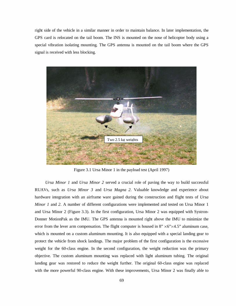
69

right side of the vehicle in a similar manner in order to maintain balance. In later implementation, the

GPS card is relocated on the tail boom. The INS is mounted on the nose of helicopter body using a

special vibration isolating mounting. The GPS antenna is mounted on the tail boom where the GPS

signal is received with less blocking.

Figure 3.1 Ursa Minor 1 in the payload test (April 1997)

Ursa Minor 1 and Ursa Minor 2 served a crucial role of paving the way to build successful

RUAVs, such as Ursa Minor 3 and Ursa Magna 2. Valuable knowledge and experience about

hardware integration with an airframe ware gained during the construction and flight tests of Ursa

Minor 1 and 2. A number of different configurations were implemented and tested on Ursa Minor 1

and Ursa Minor 2 (Figure 3.3). In the first configuration, Ursa Minor 2 was equipped with Systron-

Donner MotionPak as the IMU. The GPS antenna is mounted right above the IMU to minimize the

error from the lever arm compensation. The flight computer is housed in 8” 6”4.5” aluminum case,

which is mounted on a custom aluminum mounting. It is also equipped with a special landing gear to

protect the vehicle from shock landings. The major problem of the first configuration is the excessive

weight for the 60-class engine. In the second configuration, the weight reduction was the primary

objective. The custom aluminum mounting was replaced with light aluminum tubing. The original

landing gear was restored to reduce the weight further. The original 60-class engine was replaced

with the more powerful 90-class engine. With these improvements, Ursa Minor 2 was finally able to

Two 2.5 kg weights

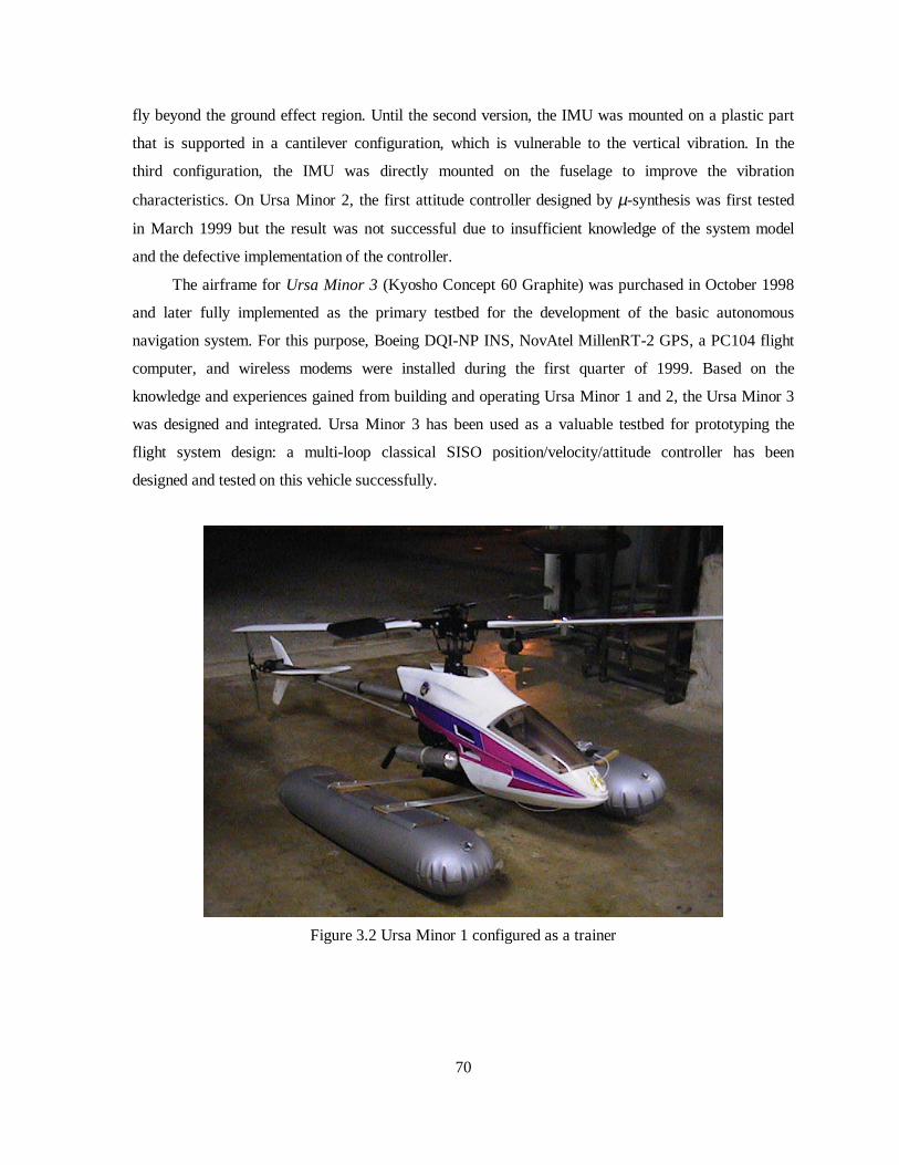
70

fly beyond the ground effect region. Until the second version, the IMU was mounted on a plastic part

that is supported in a cantilever configuration, which is vulnerable to the vertical vibration. In the

third configuration, the IMU was directly mounted on the fuselage to improve the vibration

characteristics. On Ursa Minor 2, the first attitude controller designed by µ-synthesis was first tested

in March 1999 but the result was not successful due to insufficient knowledge of the system model

and the defective implementation of the controller.

The airframe for Ursa Minor 3 (Kyosho Concept 60 Graphite) was purchased in October 1998

and later fully implemented as the primary testbed for the development of the basic autonomous

navigation system. For this purpose, Boeing DQI-NP INS, NovAtel Mill enRT-2 GPS, a PC104 flight

computer, and wireless modems were installed during the first quarter of 1999. Based on the

knowledge and experiences gained from building and operating Ursa Minor 1 and 2, the Ursa Minor 3

was designed and integrated. Ursa Minor 3 has been used as a valuable testbed for prototyping the

flight system design: a multi-loop classical SISO position/velocity/attitude controller has been

designed and tested on this vehicle successfully.

Figure 3.2 Ursa Minor 1 configured as a trainer

71

(a) February 1999

(b) April 1999

(c) August 1999

Figure 3.3 Ursa Minor 2 in different configurations

72

Figure 3.4 Ursa Minor 3 based on Kyosho Concept 60SR II Graphite

(Configuration as of August 1999)

Wireless modemEnclosure

Boeing DQI-NP

Radio receiver

Flight Computer

GPS Unit

GPS Antenna

Vibration isolationMounting

Reinforced landing gear

Bell-Hiller Stabilizer

73

3.1.2 Ursa Major Series-Bergen Industrial Twin

The Bergen Industrial Twin is essentially a heavily modified 60-class helicopter powered by

two 2-cycle gasoline engines. Two identical engines are attached together through a custom crankcase

to generate massive horsepower. The vehicle has an oversized main rotor for additional payload. The

tailboom is significantly elongated to compensate the increased anti-torque of the main rotor. This

mutated helicopter can be the answer to the demands for higher payload helicopters at an affordable

price. The payload of the Bergen helicopter is known to be around 10 kg, which is sufficient to carry

the basic navigation system as well as some additional sensors such as a camera and ultrasonic

sensors to name a few. However, the load factor on the main rotor shaft and the control linkages is

expected to be dangerously high because the shafts and linkages are originally designed for 60 class

helicopters weighing 5-6 kg at most while typical RUAV based on Bergen would weight around 15-

20kg. Nonetheless, a number of successful RUAV implementations have been reported. For our

research, we find Bergen helicopters as a reasonable platform for vision-based ship deck landing

experiments because the host vehicle offers enough payload to carry a vision processing computer

and a camera as well as the flight control computer. For this application, a special shock-absorbing

landing gear is employed as shown in Figure 3.5.

Figure 3.5 Bergen Industrial Twin helicopter with shock absorbing landing gear

74

3.1.3 Ursa Magna Series-Yamaha R-50

Yamaha R-50 was originally developed in Japan as an efficient alternative for pesticide

spraying in rice fields. Reflecting this design concept, the helicopter features rugged construction,

simple operation, and easier control characteristics. It has high-clearance skid-type landing gear to

allow the mounting of chemical dispensing pumps. This space is ideal for mounting our custom

onboard avionics. The R-50 is powered by a water-cooled, single cylinder, 12-hp, 98 cc two-stoke

gasoline engine. The engine requires a special external engine starter. The engine is very reliable and

it is powerful enough to carry 20 kg of payload. Thanks to the ample payload, it serves as a platform

for very extensive and versatile RUAV applications.

The control system consists of five servomotors: three for the actuation of the main rotor

collective/cyclic pitches, one for the tail rotor collective pitch, and one for the engine throttle control.

Unlike Kyosho, the swashplate is actuated by a coordinated motion of three servos, i.e., left, right,

and back straight servos. The main rotor collective and cyclic pitch control obeys the following

relationship with the servo action and the obtained pitches:

( )( )

( )

2

2

2

LSS RSS

BSS LSS RSS

LSS RSS

Collective pitch L L

Longitudinal cyclic picth L L L

Lateral cyclic pitch L L

= +

= − +

= −

(3.1)

where

LSS: Left straight servo

RSS: Right straight servo

BSS: Back straight servo

Figure 3.6 The servomotor configuration for swashplate actuation of Yamaha R-50

LSS RSS

BSS

Tail servoEngine throttle servo

ReceiverBattery

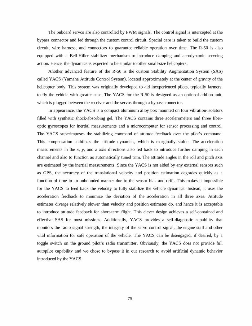
75

The onboard servos are also controlled by PWM signals. The control signal is intercepted at the

bypass connector and fed through the custom control circuit. Special care is taken to build the custom

circuit, wire harness, and connectors to guarantee reliable operation over time. The R-50 is also

equipped with a Bell-Hill er stabili zer mechanism to introduce damping and aerodynamic servoing

action. Hence, the dynamics is expected to be similar to other small-size helicopters.

Another advanced feature of the R-50 is the custom Stabili ty Augmentation System (SAS)

called YACS (Yamaha Attitude Control System), located approximately at the center of gravity of the

helicopter body. This system was originally developed to aid inexperienced pilots, typically farmers,

to fly the vehicle with greater ease. The YACS for the R-50 is designed as an optional add-on unit,

which is plugged between the receiver and the servos through a bypass connector.

In appearance, the YACS is a compact aluminum alloy box mounted on four vibration-isolators

fill ed with synthetic shock-absorbing gel. The YACS contains three accelerometers and three fiber-

optic gyroscopes for inertial measurements and a microcomputer for sensor processing and control.

The YACS superimposes the stabili zing command of attitude feedback over the pilot’s command.

This compensation stabili zes the attitude dynamics, which is marginally stable. The acceleration

measurements in the x, y, and z axis directions also fed back to introduce further damping in each

channel and also to function as automatically tuned trim. The attitude angles in the roll and pitch axis

are estimated by the inertial measurements. Since the YACS is not aided by any external sensors such

as GPS, the accuracy of the translational velocity and position estimation degrades quickly as a

function of time in an unbounded manner due to the sensor bias and drift. This makes it impossible

for the YACS to feed back the velocity to fully stabilize the vehicle dynamics. Instead, it uses the

acceleration feedback to minimize the deviation of the acceleration in all three axes. Attitude

estimates diverge relatively slower than velocity and position estimates do, and hence it is acceptable

to introduce attitude feedback for short-term flight. This clever design achieves a self-contained and

effective SAS for most missions. Additionally, YACS provides a self-diagnostic capabili ty that

monitors the radio signal strength, the integrity of the servo control signal, the engine stall and other

vital information for safe operation of the vehicle. The YACS can be disengaged, if desired, by a

toggle switch on the ground pilot’s radio transmitter. Obviously, the YACS does not provide full

autopilot capabili ty and we chose to bypass it in our research to avoid artificial dynamic behavior

introduced by the YACS.

76

Figure 3.7 Ursa Magna 2 based on Yamaha R-50 industrial helicopter

WaveLAN antennae

GPS antenna

AvionicsCamera

UltrasonicSensor

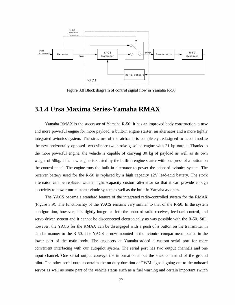
77

ReceiverR-50

Dynamics

Pilo tCom mand

PW MServomotors

Inertia l sensors

YACSComputer

PW M

YA CSActivationCom mand

YACS

Figure 3.8 Block diagram of control signal flow in Yamaha R-50

3.1.4 Ursa Maxima Series-Yamaha RMAX

Yamaha RMAX is the successor of Yamaha R-50. It has an improved body construction, a new

and more powerful engine for more payload, a built-in engine starter, an alternator and a more tightly

integrated avionics system. The structure of the airframe is completely redesigned to accommodate

the new horizontally opposed two-cylinder two-stroke gasoline engine with 21 hp output. Thanks to

the more powerful engine, the vehicle is capable of carrying 30 kg of payload as well as its own

weight of 58kg. This new engine is started by the built-in engine starter with one press of a button on

the control panel. The engine runs the built-in alternator to power the onboard avionics system. The

receiver battery used for the R-50 is replaced by a high capacity 12V lead-acid battery. The stock

alternator can be replaced with a higher-capacity custom alternator so that it can provide enough

electricity to power our custom avionic system as well as the built-in Yamaha avionics.

The YACS became a standard feature of the integrated radio-controlled system for the RMAX

(Figure 3.9). The functionality of the YACS remains very similar to that of the R-50. In the system

configuration, however, it is tightly integrated into the onboard radio receiver, feedback control, and

servo driver system and it cannot be disconnected electronically as was possible with the R-50. Still ,

however, the YACS for the RMAX can be disengaged with a push of a button on the transmitter in

similar manner to the R-50. The YACS is now mounted in the avionics compartment located in the

lower part of the main body. The engineers at Yamaha added a custom serial port for more

convenient interfacing with our autopilot system. The serial port has two output channels and one

input channel. One serial output conveys the information about the stick command of the ground

pilot. The other serial output contains the on-duty duration of PWM signals going out to the onboard

servos as well as some part of the vehicle status such as a fuel warning and certain important switch

78

positions on the radio transmitter of the ground pilot. Custom servo control can be performed by

pushing a pushbutton on the transmitter and then writing a certain value in the predefined structure

for the outgoing stream of serial port. Using serial communication for servo actuation eliminates

sources of malfunctions such as exposed PWM signal li nes, custom circuits, wire harness and

connectors. It should be noted, however, that the serial communication introduces a significant time

delay of approximately 14ms, which is 70% of the sampling time (20ms), when sending and receiving

a data packet with the YACS, respectively. This substantial amount of phase delay may cause

degradation of control performance and imposes a limit on the closed-loop bandwidth.

(a) Inertial sensor unit for YACS

(b) YACS processor enclosure with special interface connector

Figure 3.9 YACS system for Yamaha RMAX

79

The rotor head features rigid blade grippers with a pre-built fixed coning angle. While the

length of the blades is almost same with the R-50, probably to retain transportabili ty, the width is

significantly increased to generate more lift. This yields a higher disc loading. Other than this

modification to meet the higher payload rating, the linkage and control mechanism is almost identical

to that of the R-50.

The ample payload and other useful features such as the built-in starter and onboard alternator,

allow the building of an RUAV capable of fully automatic operation for an extensive amount of time.

The current plan is to build the RMAX to be able to start the operation with an automatic engine start

and carry out the given mission over a longer period of time with a high-capacity fuel tank. The

RUAV will be able to land, stop the engine automatically, and then resume the operation.

Figure 3.12 shows three Berkeley RUAVs constructed during the last two years. Ursa Maxima

2 will soon undergo a series of test flight for onboard system reliabili ty, system identification, and

controller design.

Figure 3.10 Detailed views of Yamaha RMAX

LSS RSS

BSS

Engine block

Receiver SW

Receiver/YACS

EngineStart SW

Bell-Hiller Rotorhead

80

Figure 3.11 Ursa Maxima 2 based on Yamaha RMAX industrial helicopter

Avionics

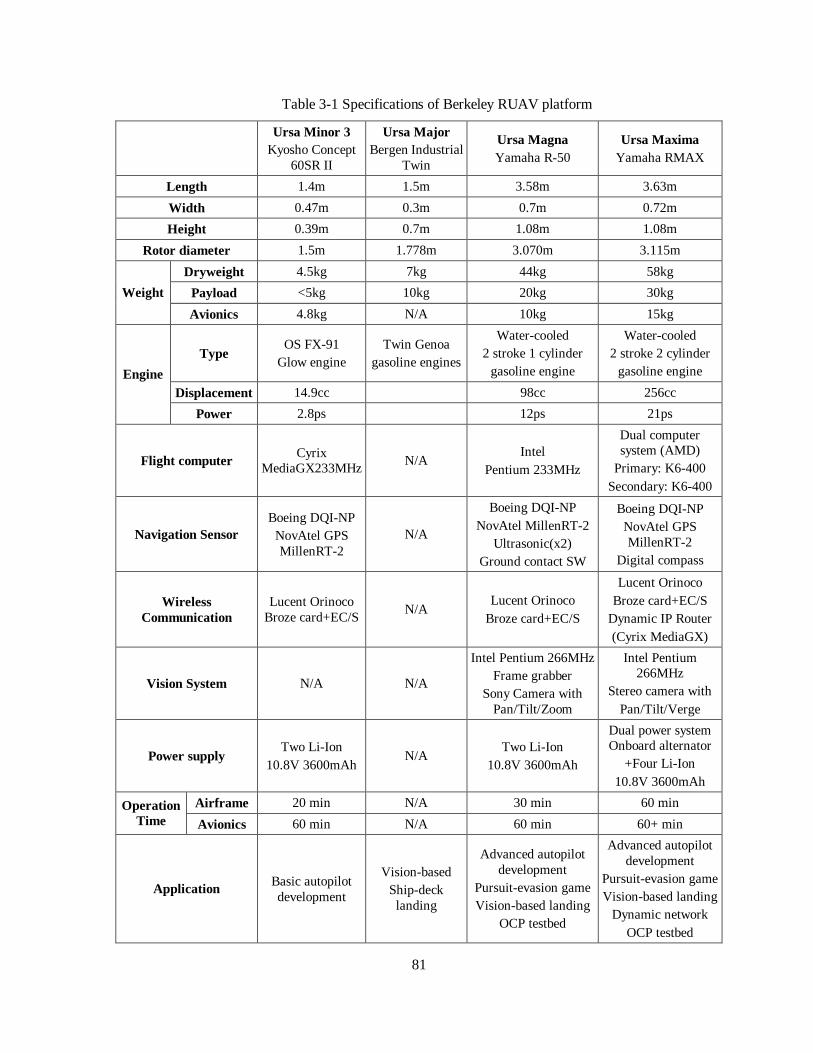
81

Table 3-1 Specifications of Berkeley RUAV platform

Ursa Minor 3

Kyosho Concept 60SR II

Ursa Major Bergen Industrial

Twin

Ursa Magna Yamaha R-50

Ursa Maxima Yamaha RMAX

Length 1.4m 1.5m 3.58m 3.63m

Width 0.47m 0.3m 0.7m 0.72m

Height 0.39m 0.7m 1.08m 1.08m

Rotor diameter 1.5m 1.778m 3.070m 3.115m

Dryweight 4.5kg 7kg 44kg 58kg

Payload <5kg 10kg 20kg 30kg Weight

Avionics 4.8kg N/A 10kg 15kg

Type OS FX-91

Glow engine Twin Genoa

gasoline engines

Water-cooled 2 stroke 1 cylinder

gasoline engine

Water-cooled 2 stroke 2 cylinder

gasoline engine

Displacement 14.9cc 98cc 256cc Engine

Power 2.8ps 12ps 21ps

Flight computer Cyrix

MediaGX233MHz N/A

Intel Pentium 233MHz

Dual computer system (AMD)

Primary: K6-400 Secondary: K6-400

Navigation Sensor Boeing DQI-NP NovAtel GPS MillenRT-2

N/A

Boeing DQI-NP NovAtel MillenRT-2

Ultrasonic(x2) Ground contact SW

Boeing DQI-NP NovAtel GPS MillenRT-2

Digital compass

Wireless Communication

Lucent Orinoco Broze card+EC/S

N/A Lucent Orinoco

Broze card+EC/S

Lucent Orinoco Broze card+EC/S

Dynamic IP Router (Cyrix MediaGX)

Vision System N/A N/A

Intel Pentium 266MHz Frame grabber

Sony Camera with Pan/Tilt/Zoom

Intel Pentium 266MHz

Stereo camera with Pan/Tilt/Verge

Power supply Two Li-Ion

10.8V 3600mAh N/A

Two Li-Ion 10.8V 3600mAh

Dual power system Onboard alternator

+Four Li-Ion 10.8V 3600mAh

Airframe 20 min N/A 30 min 60 min Operation Time Avionics 60 min N/A 60 min 60+ min

Application Basic autopilot development

Vision-based Ship-deck landing

Advanced autopilot development

Pursuit-evasion game Vision-based landing

OCP testbed

Advanced autopilot development

Pursuit-evasion game Vision-based landing

Dynamic network OCP testbed

82

Figure 3.12 Fully equipped RUAV fleet at UC Berkeley

(left to right: Ursa Magna 2, Ursa Minor3 , Ursa Maxima 2)

3.2 Navigation and Control System

The Flight Control System (FCS) is the onboard component that is responsible for the overall

vehicle management tasks such as vehicle guidance, control and communication. The main task of

the flight computer is, as once put very eloquently, to 1) aviate, 2) navigate, and 3) communicate. In

other words, the vehicle should be able to sustain its flight by proper stabili zation and control of the

vehicle dynamics and then should be guided along the desired waypoints and trajectories. Finally, the

vehicle should communicate with the ground monitoring station and other aerial or ground-based

agents if presented or required. Hence, the flight computer should 1) manage the sensor system, 2)

stabili ze and control the host vehicle at a low or high-level, and 3) communicate with other agents of

the entire UAV system including the ground station. Among the many aspects of the operation of the

flight computer, the realtime performance is one of the most important parts. In the following, a

detailed description of the flight control system is given at the component level.

83

3.2.1 Flight Computer System

The flight computers used in this research are PC-compatibles in the PC104 standard. Although

PC compatibles were not designed for a realtime control tasks, they can achieve a decent realtime

performance when combined with realtime timing circuitry and a meticulous scheduling algorithm. A

flight computer typically consists of one CPU board and other peripheral boards such as RS-232/422

communication board, Ethernet board, PWM generation board, DC-DC power supply and so on. In

this research, the PC boards complying with the PC104 industrial standard are chosen due to their

higher level of reliabili ty and robustness than normal desktop boards, their wide variety of supporting

functions, and their availabili ty. The PC104 features a 3.55”3.775” footprint circuit board that has

the ISA bus or sometimes with the PCI bus of the Intel x86 based PCs (the system with PCI bus is

called PC104-plus). The only difference is the shape of the ISA bus connector. The boards are

interconnected through the PC104 bus, which is almost identical to ISA bus with a different

connector of 104 pins (hence the name). The CPU board is expanded by other peripheral boards and

forms a stack as shown in Figure 3.13. This configuration accomplishes more ruggedness and

reliabili ty than the standard motherboard-daughterboard configuration found in desktop computers.

Figure 3.13. PC 104 stack (flight computer for Ursa Minor 3)

84

In this research, slightly different combinations of PC104 cards are used for each RUAV

depending on their payload and application. More powerful CPUs are usually desired for improved

realtime performance and future expandabili ty. For the Kyosho Concept series helicopters, where the

payload is the most limiting factor in the design, smaller CPU boards are preferred. In the beginning

of the research back in 1996, a 586 CPU running at 133MHz was adopted for the Ursa Minor 1. Later

it is replaced with a Pentium 233MHz because the 586 board could not handle the realtime

computational load of the INS/GPS integration algorithm. The Pentium board used in this research is

in the 8”6” “Littleboard” format, which is in fact larger and heavier than a normal PC104 board and

offers more onboard peripherals such as four serial ports, SCSI, dual IDE, a video adapter and a

10BaseT Ethernet port. For Ursa Minor 3, a standard PC104 CPU board with a Cyrix MediaGX

233MHz is used because of its smaller size and improved speed over the early 586 CPU.

For Ursa Magna 2, whose payload is not a limiting factor at all, a heavier and more powerful

Littleboard from Ampro is used again because Pentium offers the fastest floating-point computation.

For Ursa Maxima 2, more ambitious configuration of multiple flight computers for advanced flight

control is laid out. Two AMD K6-400MHz CPU boards called Panther board1 in standard PC104

format are used because their smaller footprint enables a multiple CPU configuration in a slightly

larger enclosure than that of R50. The Panther board shows execution speed comparable with that of

Pentium 233MHz. Because the floating point unit of AMD K6-400 is known to be slower than that of

the Pentium running at the same clock speed. The latest AMD board consists of two PC104 boards

featuring many useful peripheral ports including solid-state disk (SSD) support, two serial ports, two

USB ports, one 10BaseT Ethernet port and one IDE interface.

Table 3-2 shows that the flight computer systems for different helicopters have many peripheral

boards in common. The main difference comes from the configuration of the base CPU board. For

Ursa Minor 3 and Ursa Magna 2, the counter/timer card and custom take-over boards are commonly

used for PWM signal reading and generation. Serial port expanders are commonly used by all

configurations because many navigation sensors communicate via serial port.

The flight computer needs hard drive or some other equivalent mass-storage device for booting

and running an operating system. Solid-state devices are preferred for their robustness against severe

vibration. The DiskOnChip™ by M-Systems is a flash RAM device and is suitable for this type of

operational environment. They are used on the MediaGX board and the Panther™ AMD boards.

Ampro Littleboards do not support DiskOnChip currently and the PCMCIA FlashDisk card is used

instead through a special adapter card.

1 Versalogic Inc. (http://www.versalogic.com)

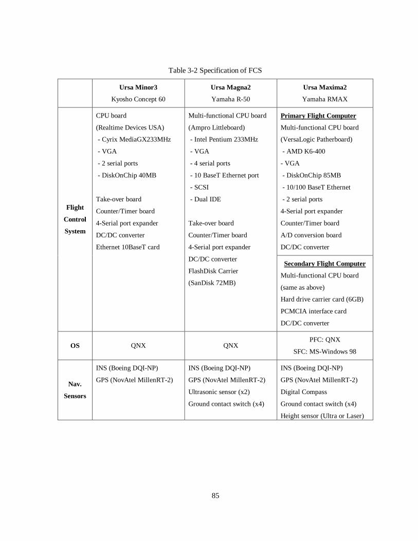
85

Table 3-2 Specification of FCS

Ursa Minor3

Kyosho Concept 60

Ursa Magna2

Yamaha R-50

Ursa Maxima2

Yamaha RMAX

Primary Flight Computer

Multi-functional CPU board

(VersaLogic Patherboard)

- AMD K6-400

- VGA

- DiskOnChip 85MB

- 10/100 BaseT Ethernet

- 2 serial ports

4-Serial port expander

Counter/Timer board

A/D conversion board

DC/DC converter

Flight

Control

System

CPU board

(Realtime Devices USA)

- Cyrix MediaGX233MHz

- VGA

- 2 serial ports

- DiskOnChip 40MB

Take-over board

Counter/Timer board

4-Serial port expander

DC/DC converter

Ethernet 10BaseT card

Multi-functional CPU board

(Ampro Littleboard)

- Intel Pentium 233MHz

- VGA

- 4 serial ports

- 10 BaseT Ethernet port

- SCSI

- Dual IDE

Take-over board

Counter/Timer board

4-Serial port expander

DC/DC converter

FlashDisk Carrier

(SanDisk 72MB)

Secondary Flight Computer

Multi-functional CPU board

(same as above)

Hard drive carrier card (6GB)

PCMCIA interface card

DC/DC converter

OS QNX QNX PFC: QNX

SFC: MS-Windows 98

Nav.

Sensors

INS (Boeing DQI-NP)

GPS (NovAtel MillenRT-2)

INS (Boeing DQI-NP)

GPS (NovAtel MillenRT-2)

Ultrasonic sensor (x2)

Ground contact switch (x4)

INS (Boeing DQI-NP)

GPS (NovAtel MillenRT-2)

Digital Compass

Ground contact switch (x4)

Height sensor (Ultra or Laser)

86

BoeingDQI-NP

INS

NovAtelGPS

MillenRT-2

LucentOrinoco

EC/S

RS-232115200 8N1

RS-232

9600 8N1

RS-232115200 8N1

Ethernet

RS

-23

21

15

20

0 8

N1

RS-2329600 8N1

RS-232115200 8N1

DigitalCompass

UltrasonicsArray

VisionComputer

RS-2329600 8N2

Main Memory

PC

I B

us

ISA

Bu

s (8

MH

z, 8

/16

bits

)C

PU

Bu

s

X-Bus

(8MHz,8/16bits)

Onboard Com puterw it h PCI local bu s

Memorycontroller

System ROM

Expansionbus controller

Buffer

RTC

Keyboardcontroller

Interruptcontroller

DMA

Systemtimer

PCI buscontroller

CPUPentium orCompatible

EthernetInterface

Counter/Timer/

DIOCard

ElectricalSingals

CustomTake-over

Board

Receiver

UARTSerial port

Driver

Servomotors

Figure 3.14 Interconnection diagram of onboard flight computer based on PCI local bus

(Ursa Magna 2)

87

In Figure 3.14, the interconnection diagram of the onboard flight computer and other sensors is

shown. Serial port communication constitutes the backbone of inter-device connection. In this

research, RS-232, which uses single-ended transmission/reception lines and supplementary control

lines, is universally used instead of RS-422, which uses differential voltage signal li nes. All flight

computers are equipped with a 4-port serial port expansion board so as to accommodate the

demanded number of serial ports. In the hardware as well as the software aspect, it is very important

to understand how the serial communication works. Since the data is decoded and transferred as a

stream of bits accompanied by a start bit, stop bit(s) and in some cases parity bits, it takes longer than

parallel ports to transfer the same amount of data. Also, the transmission time for 1 bit is limited by

1/115200 second that is longer than other protocols such as USB (Universal Serial Bus) or Ethernet,

and hence the overall communication time causes delay which degrades realtime performance. The

actual realtime performance measured in Ursa Magna 2 will be given in Section 3.5.

3.2.2 Navigation Sensors

To navigate following a given trajectory while stabili zing the vehicle, the information about

vehicle position, velocity, attitude, and angular rates should be known to the guidance and control

system. The RUAVs are equipped with a number of complementary navigation sensors to obtain

accurate information about the motion of the vehicle in association with environmental information,

such as the relative distance to the ground surface to other objects near the vehicle.

The navigation sensors can be categorized as (1) environment-independent sensors and (2)

environment-dependent sensors. The former includes INS and GPS, which compute the motion

estimates regardless of the surrounding. The latter includes ultrasonic sensors, laser range finders and

vision sensors. These sensors rely on the surrounding objects, which reflect the active probing signals

such as an ultrasonic wave or laser beam, or on natural li ghts to form an image on the CCD receptors

of the camera. These sensors are necessary to determine the relative distance from the vehicle to its

surrounding objects or the ground surface for take-off/landing, colli sion avoidance or evasive

maneuvers. The characteristics of these sensors are reviewed in the following sections.

88

3.2.2.1 Inertial Navigation System

The inertial navigation system is the central part of the navigation sensor system of the

Berkeley RUAV system. Inertial navigation is a method which provides the motion estimates such as

position, velocity and attitude by processing the inertial quantities sensed by inertial instruments. An

INS consists of three accelerometers and three gyroscopes which measure the linear acceleration and

angular rates. There are two types of INS: the mechanized-platform type and the strap-down type.

The former consists of a mechanized gimbal platform, which aligns itself consistently along the

reference inertial coordinate system regardless of the base vehicle’s attitude change. The

accelerometers are mounted on this platform. The velocity in the inertial coordinate system can be

easily found by integration in each channel. The overall accuracy of the sensor system depends on the

alignment of the instrument platform. The alignment requires a very precise sensing and actuation ot

the mechanism. The strap-down type of INS utili zes three accelerometers and three rate gyroscopes,

which are installed in the precise orthogonal x, y, and z direction. The inertial measurement unit is

mounted on the vehicle without any actuation, and hence the inertial quantities are measured in the

body-coordinate system. Transforming the inertial estimates into the spatial coordinates becomes the

full responsibili ty of the inertial processing unit of the strap-down type INS. This process involves the

integration of the accelerations measured in the body coordinate frame as well as the transformation

into the spatial coordinates using the estimated Euler angles or other equivalents. The attitude angles

are estimated by numerically integrating the differential equations in equation (2.11) or (2.13). In

summary, the inertial estimates can be found by the following equation:

1 2 3 4( , , , )

TP

TP bB TP q q q q→

=

=

=

P V

V R A

q T

(3.2)

The equations in (3.2) are pure kinematical relationships which hold true. However, the actual

numerical integration is far less than ideal due to many error sources such as bias, drift, scaling error

of the inertial sensors, imperfect integration by numerical algorithms and so forth. Hence, equation

(3.2) should be augmented with a dynamic error model to minimize the deviation of the solution as

time lapses. All the measurements of linear acceleration and angular rates are contaminated by noise,

scaling error, bias and drift. Without proper calibration and compensation, the inertial estimates

diverge very quickly. These error sources have a stochastic nature, and hence the unit should be

89

initialized every time it is turned on. The best method of initialization is to measure the accelerations

while keeping the unit stationary, in all channels, and calibrate them by comparing the values with the

gravitational force. Unfortunately, the noise characteristics of these sensors change after the

initialization. The bias swing, known as drift, slowly changes over time as a function of many factors,

including the temperature. Therefore, high-accuracy INS cannot be built without the proper

initialization and continuous compensation of the drift. While initial roll and pitch angles can be

estimated approximately by computing the inclination angles using the measurements of the

acceleration caused by the gravitational force, the initial heading is not observable at all by the inertial

measurements. External information should be provided from such aids as heading sensors. This

process is called the alignment process. The calibration and alignment processes can be performed

without leaving the sensor unit stationary by using accurate external sensors such as GPS. If GPS is

used, the sensor unit should be moved around so that the inertial estimates can be compared with GPS

and then used for inertial sensor calibration.

The strap-down IMU is the main trend these days. They are particularly suitable for small-size

vehicle applications because they are more advantageous than the mechanized-platform INS in terms

of size and weight. The additional computational load for the strap-down system can be easily taken

care of by today’s powerful and small microprocessors. In the Berkeley RUAV research, we have

consistently used a strap-down IMU for this reason. Most small-size strap-down IMUs contain the

inertial sensors that are manufactured using micromachining and hence they are very small and light.

Accelerometers are usually made of solid-state MEMS (Micro Electro-Mechanical Systems) using

pitchfork technology. For rate gyroscopes, solid-state MEMS sensors or more accurate (and

expensive) fiber-optic gyroscopes (FOG) are used.

In the Berkeley RUAV research, except for the brief period during which a special type of INS

was investigated using six accelerometers, two types of inertial instruments have been consistently

used. At first, MotionPak™ from Systron-Donner was used. MotionPak contains three accelerometers

and three rate gyroscopes that output analog voltages. It is the user’s responsibili ty to properly

calibrate, filter the noise and compensate the bias as described above. Unfortunately, the Berkeley

UAV team could not spend enough time and effort to develop and implement the proper

compensation and alignment algorithm, and so we looked for an alternative. The Boeing DQI-NP

(Digital Quartz IMU-Navigation Processor) offers fully integrated digital signal processors (DSP) for

the full set of inertial estimates of position, velocity, and attitude as well as the raw sensor outputs of

accelerometers and rate gyroscopes. Inertial measurements are easily acquired by reading the serial

port output in the RS-232 or RS-422 protocol, which is user-selectable. Another attractive feature is

the GPS integration capabili ty: DQI-NP accepts the position update from GPS every second and

90

updates the internal Kalman filter for loosely coupled INS/GPS compensation. It supports a limited

number of GPS models and unfortunately, the GPS system used in our research, NovAtel Mill enRT-

2, is not among them for now. Therefore, an emulation program has to read the GPS output, cast it

into one of the supported GPS message format, and feed it into the DQI-NP. The detailed information

about this program will be discussed in Section 3.5

Figure 3.15 Inertial instruments: Boeing DQI-NP (left) Systron-Donner MotionPak™ (right)

Care should be taken with the mounting of DQI-NP. It is known that the inertial sensors inside

the DQI-NP sensor module has an excitation frequency of 100 Hz. Coincidently, the RPM of the tail

rotor of Ursa Minor 3 is around 6000 RPM (=100Hz) in hover and it was discovered that the

navigation solution of DQI-NP diverges frequently. This problem was solved by the special shock-

absorbing mounting for DQI-NP as shown in Figure 3.16.

Figure 3.16 Boeing INS DQI-NP installed on Ursa Minor3(left) and Ursa Magna2 (right)

91

The DQI-NP operates on a DC power source ranging between 20-34V. The Lithium-ion

batteries used for our research are rated 10.8 V and two batteries are put in series so that the overall

voltage is high enough to power the DQI-NP. The battery power source is shared with other onboard

systems such as the flight computer and other navigation sensors. For Ursa Maxima helicopters, the

input voltage for the avionics is fixed at 12V by the onboard lead-acid battery and a separate DC-DC

converter is used to escalate the 12V input to 24V for DQI-NP.

3.2.2.2 Global Positioning System

NAVSTAR GPS is a space-based satelli te radio navigation system developed by the United

States Department of Defense. GPS provides three-dimensional position and time with the deduced

estimates of velocity and heading. The GPS system consists of three major segments: Space, Control

and User. The space segment consists of 24 satelli tes in circular orbits 20,200 km above the Earth’s

surface, with a 12-hour orbital period and an inclination angle of 55 degrees. This configuration

intends to provide at least five satelli tes in view from any point on Earth at any time.

Each satelli te continuously broadcasts radio signals at two L-band frequencies: L1 at 1575.42

MHz and L2 at 1227.6 MHz. The L1 frequency contains Precise ranging signal (P-code) modulated

by 10.23 MHz as well as 1.023 MHz Coarse/Acquisition Code (C/A-code). The L2 frequency

contains P-code only, which used to be dedicated for mili tary GPS use only. L2 frequency used to be

degraded with an certain encryption, which deterred non-authorized users from obtaining the utmost

accuracy from the GPS. This process, known as Selective Availability (S/A), was known to inject as

much error as 30m. It was finally eliminated in May of 2000. In our field experience, GPS accuracy

has been significantly improved from a standard deviation of 25m to 2.5 m. The navigation data from

each satelli te contains time, clock correction, ephemeris parameters, almanac data, and health status.

Based on this information, the user segment, i.e., the GPS receiver, computes the current position of

each satelli te. Actually, the receiver computes the elapsed time of each signal set to travel the distance

from the source satelli te to the receiver antenna. Stemming from the simple concept of triangular

survey, with the additional unknown variable for time drift of the internal clock of the GPS receiver,

four measurements, i.e., at least four satelli tes are required. The distance estimated in this manner is

called the pseudorange. It earned its name because it contains errors from many sources. This

process, relying on the NAVSTAR satelli tes only for positioning, is known as Single Position Station

(SPS). Now that S/A has been eliminated, pseudoranging offers improved accuracy.

92

When two GPS systems are operated in the same vicinity, the overall accuracy of GPS can be

significantly improved by canceling the common errors of those two systems. One receiver, the

reference station, is positioned at a precisely known location and computes the pseudorange and

correction information, and broadcasts it via radio link. The rover station computes its location and

corrects it with the additional correction information it gains from the radio link. This scheme is

called differential GPS (DGPS). Significantly more accurate position is estimated if the two receivers

are located within 50 km with each other. It should be noted that precise knowledge of the position

coordinates of the reference station directly impacts the rover’s accuracy.

Further accuracy can be achieved with a method known as the carrier-phase algorithm. In this

approach, the receiver monitors the number of wavelengths that the radio signal has to travel from the

satelli te to the antenna. The L1 frequency has a wavelength of 19 cm and the L2 is 24 cm. The

distance divided by the wavelength will be the sum of an integer and a fractional component.

Determining the integer portion is not straightforward and hence it is called ambiguity. A GPS can

improve the accuracy significantly by looking for the integer using the lane search problem on both

L1 and L2 frequencies. When it is locked in the narrow-lane solution, the accuracy of the baseline,

the vector from the reference station to the rover station, can be as accurate as 1~2 cm.

The global positioning system (GPS) used in this research is the NovAtel Mill enRT-2, which

achieves this remarkable accuracy of 2cm through the use of DGPS and a carrier-phase algorithm.

The NovAtel GPS provides position estimates at up to 10 Hz. We configured the receiver to generate

the position log at 4 Hz. The flight control computer acquires the position, linear/angular velocity and

attitude from the DQI-NP, and high accuracy position estimates from the NovAtel RT-2 via RS-232.

It also relays the converted position estimate message packet from the GPS to the DQI-NP every

second.

The actual operation of GPS takes caution and sometimes can be very frustrating. Our research

used the NovAtel Mill enRT-2, which requires a couple of minutes to lock itself onto the narrow lane

solution. The necessary time for the lock-up depends on many factors such as the number of satelli tes

in the sky view, the elevation angle of the satelli tes, and the ambient radio activity near the L1 and L2

frequencies and so forth. During experiments, the GPS often causes trouble because it is not able to

sequence into the narrow-lane solution in a reasonable time. Theoretically, the floating-point solution

can still be used as the position estimates. The only problem is that the position estimates have sudden

jumps whenever the solution type changes. This may cause undesirable transient behavior in the INS,

and if the loop is closed, the control system would react to this sudden jump and produce large jump

in the control output. Therefore, fail-safety coding should be programmed for guaranteed operation.

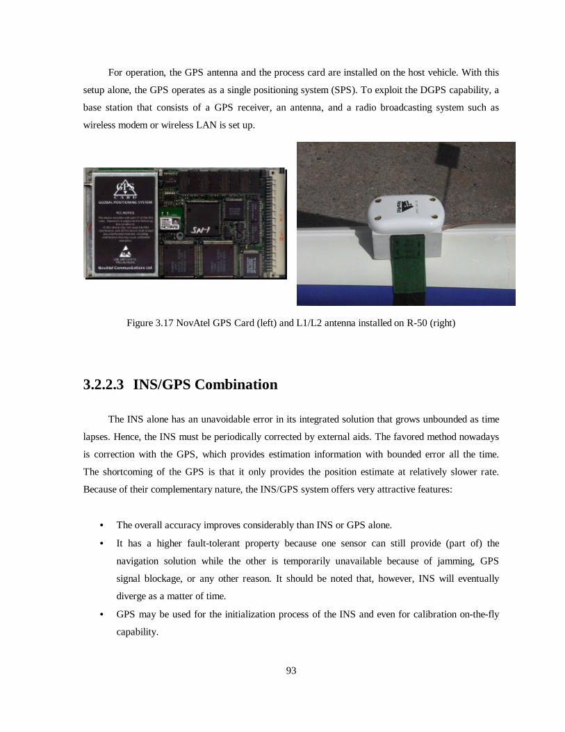
93

For operation, the GPS antenna and the process card are installed on the host vehicle. With this

setup alone, the GPS operates as a single positioning system (SPS). To exploit the DGPS capabili ty, a

base station that consists of a GPS receiver, an antenna, and a radio broadcasting system such as

wireless modem or wireless LAN is set up.

Figure 3.17 NovAtel GPS Card (left) and L1/L2 antenna installed on R-50 (right)

3.2.2.3 INS/GPS Combination

The INS alone has an unavoidable error in its integrated solution that grows unbounded as time

lapses. Hence, the INS must be periodically corrected by external aids. The favored method nowadays

is correction with the GPS, which provides estimation information with bounded error all the time.

The shortcoming of the GPS is that it only provides the position estimate at relatively slower rate.

Because of their complementary nature, the INS/GPS system offers very attractive features:

• The overall accuracy improves considerably than INS or GPS alone.

• It has a higher fault-tolerant property because one sensor can still provide (part of) the

navigation solution while the other is temporarily unavailable because of jamming, GPS

signal blockage, or any other reason. It should be noted that, however, INS will eventually

diverge as a matter of time.

• GPS may be used for the initialization process of the INS and even for calibration on-the-fly

capabili ty.

94

When the INS is integrated with the GPS, the INS accepts the position measurement from GPS

updates at slower rates. The Kalman filter integrates the raw inertial sensor measurements and

corrects its solution with the GPS position updates. The combinatory system outputs the compensated

position, velocity, and attitude estimates at high speed with bounded error.

There are two types of integration of INS/GPS [36]: loosely-coupled GPS aided INS and

tightly-coupled GPS aided INS. In the former approach, only the position or range information from

the GPS is fed into the INS to correct the position estimates. This method is computationally light and

easy to implement. In the latter scheme, the acceleration information from INS is used by the carrier-

tracking loop and this improves the signal-to-noise ratio and makes the overall system more robust to

jamming and interference. While the latter may be more effective, it requires a full access to INS and

GPS. This is not usually possible when using COTS INS and GPS.

DQI-NP provides loosely coupled GPS integration. In our experience, the performance of DQI-

NP is acceptable when it is used in INS/GPS combination. One major deficiency of the DQI-NP is

that it is impossible to specify that the standard deviation of position error is less than 1 meter because

the data field for this information is defined as an integer variable in meter. In addition, the position

update from DQI is 1Hz, which is too slow for high-accuracy position control. Therefore, an

additional Kalman filter is implemented on the flight computer in order to generate high-speed

position updates at 50 Hz. The Kalman filter performs numerical integration of the velocity estimates

of the DQI-NP and correct it with the GPS measurements, which are available at 4Hz.

Since it is impossible to install the antenna and the IMU at the same location, there is always

the offset between these two points. Therefore, the position of GPS should be compensated for the

offset to the INS position. These two positions have a fixed distance if we assume they are attached to

a rigid body. This distance is called lever-arm and its compensation involves the transformation

between the body coordinate system and the inertial coordinate system such that

INS GPS GPS INSTP TP B TP B

→→= +X X R X (3.3)

where

GPSTPX : GPS location in the inertial frame

INSTPX : INS location in the inertial frame

GPS INSB

→X : the relative coordinate of INS with respect

to GPS in the body coordinate system

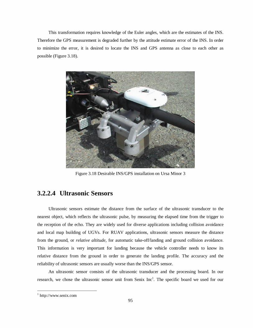
95

This transformation requires knowledge of the Euler angles, which are the estimates of the INS.

Therefore the GPS measurement is degraded further by the attitude estimate error of the INS. In order

to minimize the error, it is desired to locate the INS and GPS antenna as close to each other as

possible (Figure 3.18).

Figure 3.18 Desirable INS/GPS installation on Ursa Minor 3

3.2.2.4 Ultrasonic Sensors

Ultrasonic sensors estimate the distance from the surface of the ultrasonic transducer to the

nearest object, which reflects the ultrasonic pulse, by measuring the elapsed time from the trigger to

the reception of the echo. They are widely used for diverse applications including colli sion avoidance

and local map building of UGVs. For RUAV applications, ultrasonic sensors measure the distance

from the ground, or relative altitude, for automatic take-off/landing and ground colli sion avoidance.

This information is very important for landing because the vehicle controller needs to know its

relative distance from the ground in order to generate the landing profile. The accuracy and the

reliabili ty of ultrasonic sensors are usually worse than the INS/GPS sensor.

An ultrasonic sensor consists of the ultrasonic transducer and the processing board. In our

research, we chose the ultrasonic sensor unit from Senix Inc1. The specific board we used for our

1 http://www.senix.com

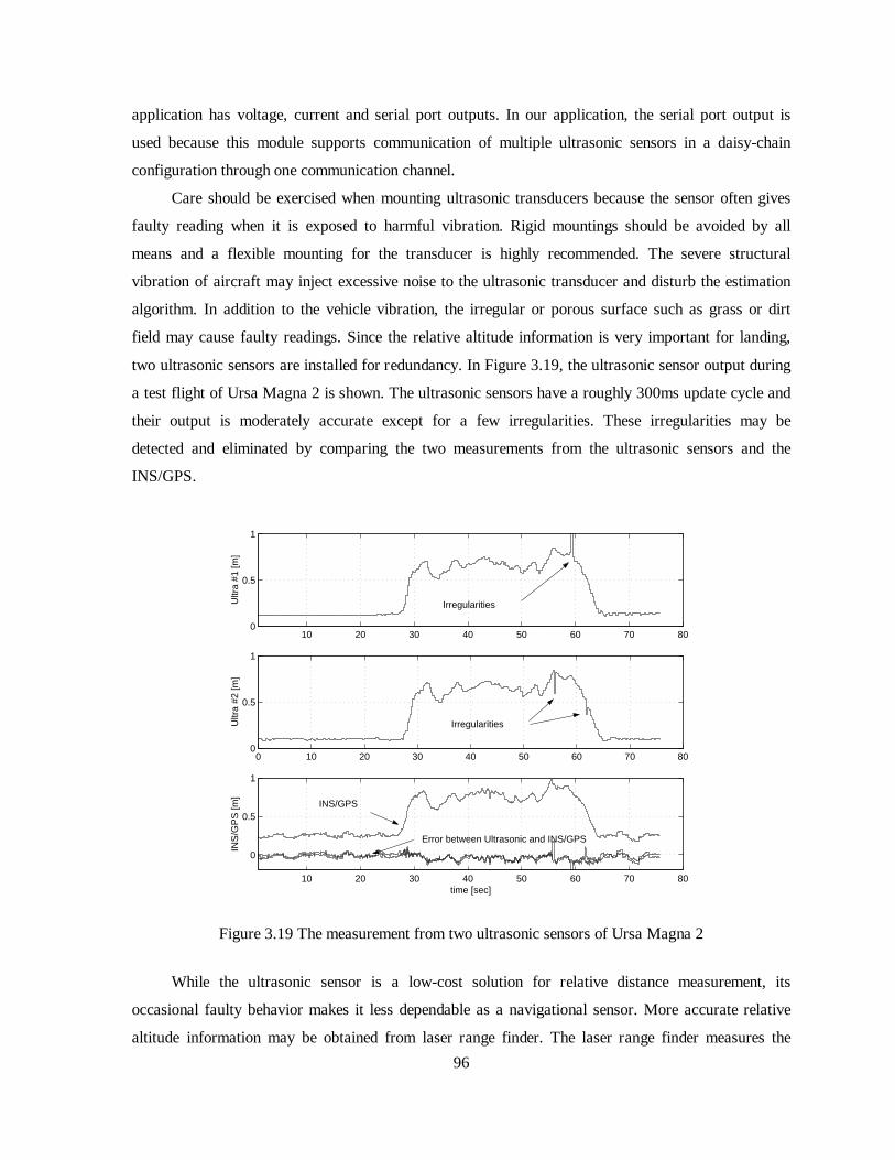
96

application has voltage, current and serial port outputs. In our application, the serial port output is

used because this module supports communication of multiple ultrasonic sensors in a daisy-chain

configuration through one communication channel.

Care should be exercised when mounting ultrasonic transducers because the sensor often gives

faulty reading when it is exposed to harmful vibration. Rigid mountings should be avoided by all

means and a flexible mounting for the transducer is highly recommended. The severe structural

vibration of aircraft may inject excessive noise to the ultrasonic transducer and disturb the estimation

algorithm. In addition to the vehicle vibration, the irregular or porous surface such as grass or dirt

field may cause faulty readings. Since the relative altitude information is very important for landing,

two ultrasonic sensors are installed for redundancy. In Figure 3.19, the ultrasonic sensor output during

a test flight of Ursa Magna 2 is shown. The ultrasonic sensors have a roughly 300ms update cycle and

their output is moderately accurate except for a few irregularities. These irregularities may be

detected and eliminated by comparing the two measurements from the ultrasonic sensors and the

INS/GPS.

10 20 30 40 50 60 70 800

0.5

1

Ultr

a #1

[m]

0 10 20 30 40 50 60 70 800

0.5

1

Ultr

a #2

[m]

10 20 30 40 50 60 70 80

0

0.5

1

time [sec]

INS

/GP

S [m

]

Irregularities

Irregularities

Error between Ultrasonic and INS/GPS

INS/GPS

Figure 3.19 The measurement from two ultrasonic sensors of Ursa Magna 2

While the ultrasonic sensor is a low-cost solution for relative distance measurement, its

occasional faulty behavior makes it less dependable as a navigational sensor. More accurate relative

altitude information may be obtained from laser range finder. The laser range finder measures the

97

distance from the laser generator to a point on the target surface by measuring the time for the laser

beam to travel back and forth between these points. Therefore, it requires highly a precise mechanical

and electrical system and is usually heavy, large, and expensive. When the laser range finder is

combined with the INS/GPS, it serves as a superb sensor for building a local geographic map.

3.2.3 Servomotor Control

The final stage of the flight control is the actuation of the servomotors installed on the

helicopter. Radio-controlled helicopters are typically equipped with five servomotors that actuate the

main rotor swash plate, the tail collective pitch yoke and the engine throttle. Usually the engine

control and the tail control are similar among helicopters, the mechanism for main rotor swashplate

differs from model to model.

A servomotor is a compact electromechanical device consisting of a DC motor with a built-in

feedback circuit. These servomotors accept pulse-width modulation (PWM) signals as the reference

input. The flight control system should be able to generate the compatible PWM signal for servo

actuation. It is also very desirable to read the incoming PWM signals from the receiver for system

identification introduced in Section 2.2.8. The detailed information of the PWM reading and

generation is listed in Appendix A.4.

3.3 Wireless Communication

Since the vehicle is operated in free space without any umbili cal cords for power or

communication, the onboard avionics should be equipped with some wireless communication device.

In the early part of the research, 900MHz wireless modems were used for avionics data

communication and DGPS correction broadcasting. Ursa Minor 1, 2 and 3 as well as Ursa Magna 2

were equipped with two wireless modems. The wireless modems used for this research are

manufactured by FreeWave Inc1. They offer very reliable communication link with throughput

somewhere between 57.6 kbps ~ 115.2 kbps. They also offer very long-range communication with a

maximum of 1 watt power. It utili zes frequency-hopping TDMA protocol and supports a number of

configurations such as master-to-slave, master-to-multiple-slave, multiple-master-to-slave and so on.

Master-to-slave is the basic configuration for one-to-one communication such as flight data

1 http://www.freewave.com

98

downloading. Master-to-multiple-slave is ideal for broadcasting DGPS corrections to multiple

numbers of vehicles with GPS system.

Although the wireless modem functioned flawlessly many times, there were three limiti ng

factors: (1) the limited bandwidth, (2) the limited protocol, and (3) possible interference with GPS.

The first two factors are the natural consequences of serial port communications. The third factor

raised curiosity because the wireless modem does not operate in the GPS L1 or L2 bands. It was

discovered that the built-in automatic gain control (AGC) amplifier of NovAtel GPS in its RF circuit

is the source of the problem. When the change of the RF activity in the neighboring bands is above

certain level, which might interfere the GPS operation, the NovAtel GPS temporarily outputs an

unusable data set with the error indication in GPS logging and resumes the normal operation as soon

as an adjustment is made. If this condition is prolonged, the GPS loses the tracking and resumes the

integer searching.

For multi-agent scenarios, one-to-one communication regime offered by radio modems is

severely restrictive to access the peer-to-peer communication protocol. The need for higher

throughput is another reason to abandon the conventional wireless serial communication. As an

alternative for the wireless modem, the Lucent WaveLAN®, later renamed to Orinoco®, is chosen.

Orinoco is a 2.4GHz wireless Ethernet system compatible with IEEE 802.11b. Packaged in a PC

Card, it is a compact, portable and very powerful solution for wireless LAN in ad-hoc mode or in

infrastructure mode. In either mode, the wireless Ethernet provides considerably faster throughput

ranging from 1Mbps to 11 Mbps. The maximum range, seriously traded off with the throughput, is

less than 1 mile depending on the efficiency of antennae. . In our application, however, the reduction

of range is not a significant issue yet because our RUAVs are operated in a confined area no larger

than half mile. Currently, all new RUAVs and UGVs are equipped with the Orinoco system for peer-

to-peer communication in multi-agent scenarios. Due to the absence of the support for Orinoco PC

card via PCMCIA bus by QNX RTOS, the card is accessed through an add-on product Ethernet and

Serial Converter (EC/S). An EC/S offers a transparent interface between the Ethernet 10BaseT port

on computer side and the Orinoco PC Card. The EC/S also offers the serial port interface and the two

data streams of Ethernet and RS-232 are multiplexed in a 2.4GHz carrier. The serial port multiplex

capabili ty is extremely useful for DGPS broadcast and simplifies the onboard communication setup.

This is especially advantageous for smaller UAV platforms with less available payloads.

In Figure 3.20, the entire communication system set up is shown. The communication system

consists of a vehicle data communication channel and the DGPS broadcasting channel. The data

channel is now based on the Orinoco system, but the 900MHz wireless modem can be operated

concurrently as long as the interference with Orinoco can be kept minimal. The DGPS broadcast is

99

now made in both the 900MHz wireless modem channel and the 2.4GHz Orinoco wireless LAN

channel because some of UGVs are equipped with a wireless modem while all of the UAVs are now

equipped with the Orinoco system only.

Figure 3.20 Communication architecture of Berkeley UAV/UGV/SMS Testbed

3.4 Ground Station

The ground station consists of a DGPS base station with broadcasting equipment and a portable

computer connected to a communication device such as a wireless modem or wireless Ethernet. The

ground station monitors and stores the flight data of the UAV and sends the navigation commands

such as controller activation/ deactivation.

The base station is a multi-functional user interface that serves as the command post, realtime

visualization station of the vehicle status, and the data logging system. The base station uses either

wireless modem through a serial port or the Orinoco system. The software runs on Microsoft

Windows 98, which is chosen for its outstanding graphics support and its compatibili ty with the

Lucent Orinoco wireless LAN system. The software consists of a number of child windows in multi-

document interface (MDI) and it displays the text-based INS/GPS status, the vehicle status, the

control buttons, the 2-D map of the experiment site, the graphics-based navigation measurement, the

control output, and the graphical display of the vehicle status. All the information is downloaded from

100

the helicopter via the wireless network and is displayed in realtime. The incoming data may be saved,

if the save option is activated, retrieved for off-line view later and exported in ASCII text form to

other applications such as MATLAB for further processing and analysis.

Figure 3.21 Ground monitoring station enhanced with GUI

3.5 Software Architecture

Vehicle management system software (VMSS) development is another very important stage for

RUAV construction. The VMSS resides in the onboard flight control computer and manages the

operation of the host RUAV. The VMSS is typically implemented on a realtime operating system

(RTOS) to guarantee the demanding hard realtime requirements. The VMSS consists of a number of

processes running at different rates to facili tate the needs of sensors and actuators. The design of the

VMSS is closely related with the setup of the flight computer and the navigation sensors. As quoted

above, the VMSS should perform the three tasks: (1) aviate, (2) navigate, and (3) communicate. The

task of aviation in the perspective of the VMSS involves the trajectory generation and the hard

realtime feedforward/feedback control of the vehicle through the aforementioned PWM generation

circuit. The task of navigation involves initialization, calibration, acquisition and fault-toleration of

Vehicle Status/Control Station 2-D Map

Nav Sensor Status Control output Vehicle Status

INS/GPS Status

101

the various onboard navigation sensors typically through serial ports. Finally, the communication is

performed through the onboard wireless communication devices such as the wireless modem or the

wireless LAN. These three tasks interact very closely: the low-level stabili zation is activated regularly

at its sampling rate and performs the INS reading, control output calculation, and download the flight

status to the ground. This is the main loop of the VMSS and other auxili ary processes such as

INS/GPS management, ultrasonic sensor polli ng, and the communication with the vision computer

run concurrently. All of these “user processes” run on the application program interface (API) of the

host RTOS. Because of the stringent requirements of the feedback control, the realtime support of the

host OS is highly emphasized. The timing jittering should be kept in a minimal range for an accurate

discrete controller realization. Since VMSS runs many tasks at different timing rates, the OS is

desired to offer multitasking environment with synchronization and interprocess communication

(IPC) capabili ties. The support of multiple serial ports is also an important factor appears as a trivial

requirements

Since VMSS takes the full responsibili ty of a remote mission, VMSS serves as an operating

system of the vehicle/electronics/software integration. Since the target RUAV platform should

perform the given high-level mission with the minimal support from the ground operator, the onboard

system management software should perform a broad level of work from control output generation to

the complex intelli gent behavior in a robust manner. The tasks of VMSS are characterized as

following:

• Sensor management

Many onboard sensors, the DQI-NP INS and the NovAtel Mill enRT-2GPS for example, need

to be properly initialized and maintained. The DQI-NP should be started following the strict

initialization procedure and it needs position updates at a regular rate. The GPS card should also be

initiated following a certain procedure. Although GPS runs quite independently, its operation can be

erratic sometimes due to external mechanical vibration, radio activity in adjacent bands, or partial

blockage of the GPS signal. Ultrasonic sensors should be polled and read regularly by sending special

characters. The sensor readings are transferred mainly via RS-232 serial ports.

• Control output computation and signal generation

The main task of the FCS is the generation of the control output to the five servos installed on

the helicopter system. The control output is calculated using either a classical multi-loop SISO control

or a MIMO -synthesis control. Then the output values are sent to the counter board and the

corresponding PWM signal is generated and sent to the servomotors.

102

• Communication

The onboard FCS should report the flight system status to the ground station for monitoring.

The information is transferred via a wireless communication method such as wireless modem or

wireless LAN. This task also includes the onboard communication with the vision computer via RS-

232. The VMSS should satisfy the following requirements:

• Reliabili ty

Reliabili ty is one of the most important factors for successful, repeatable, and consistent

operation of a RUAV system. Any accident during the test flight caused by a unreliable flight control

software can be very disastrous because any damage to the delicate sensors/computer systems is very

costly and more importantly the rotating blades can cause lethal damage to anything in their path.

Hence, thorough validation of the flight control software should be performed before any real test

flight. The code should be able to handle any run-time errors ranging from purely software problem

(segment fault, memory overflow) to vehicle-originated faults (a severed wire connection, engine

failure).

• Real-time

Some part of the task of VMSS requires hard-realtime performance. Sampling the sensor data

and generation of the control output at every sample time with small jittering is the typical example.

The VMSS should be able to meet the realtime requirement with minimal error. There are also

numerous soft realtime tasks such as polli ng sensors and wireless communications. Even though these

kind of jobs do not require as stringent of a performance as the hard-realtime tasks, these jobs should

be processed with reasonable delay.

• Readabili ty

This applies not only to the VMSS, but also to the general software development. The software

should be readable by teammates other than the programmer him/herself for further development.

Many and proper comments are strongly recommended for future references. The software can also

be expandable whenever higher layers are added to the lower level software block.

These tasks require realtime operation to guarantee stable and reliable operation. For example,

the control output generation requires a stringent sampling at a certain rate. Hence, we need a

programming environment to guarantee acceptable realtime performance. Since the PC architecture is

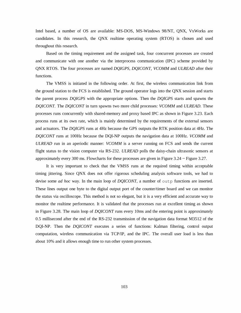
103

Intel based, a number of OS are available: MS-DOS, MS-Windows 98/NT, QNX, VxWorks are

candidates. In this research, the QNX realtime operating system (RTOS) is chosen and used

throughout this research.

Based on the timing requirement and the assigned task, four concurrent processes are created

and communicate with one another via the interprocess communication (IPC) scheme provided by

QNX RTOS. The four processes are named DQIGPS, DQICONT, VCOMM and ULREAD after their

functions.

The VMSS is initiated in the following order. At first, the wireless communication link from

the ground station to the FCS is established. The ground operator logs into the QNX session and starts

the parent process DQIGPS with the appropriate options. Then the DQIGPS starts and spawns the

DQICONT. The DQICONT in turn spawns two more child processes: VCOMM and ULREAD. These

processes runs concurrently with shared-memory and proxy based IPC as shown in Figure 3.23. Each

process runs at its own rate, which is mainly determined by the requirements of the external sensors

and actuators. The DQIGPS runs at 4Hz because the GPS outputs the RTK position data at 4Hz. The

DQICONT runs at 100Hz because the DQI-NP outputs the navigation data at 100Hz. VCOMM and

ULREAD run in an aperiodic manner: VCOMM is a server running on FCS and sends the current

flight status to the vision computer via RS-232. ULREAD polls the daisy-chain ultrasonic sensors at

approximately every 300 ms. Flowcharts for these processes are given in Figure 3.24 ~ Figure 3.27.

It is very important to check that the VMSS runs at the required timing within acceptable

timing jittering. Since QNX does not offer rigorous scheduling analysis software tools, we had to

devise some ad hoc way. In the main loop of DQICONT, a number of outp functions are inserted.

These lines output one byte to the digital output port of the counter/timer board and we can monitor

the status via oscill oscope. This method is not so elegant, but it is a very efficient and accurate way to

monitor the realtime performance. It is validated that the processes run at excellent timing as shown

in Figure 3.28. The main loop of DQICONT runs every 10ms and the entering point is approximately

0.5 milli second after the end of the RS-232 transmission of the navigation data format M3512 of the

DQI-NP. Then the DQICONT executes a series of functions: Kalman filtering, control output

computation, wireless communication via TCP/IP, and the IPC. The overall user load is less than

about 10% and it allows enough time to run other system processes.

104

File systemFsys

Device DriverDev

TTY DriverDev.ansi

Network D riverNet

EthernetDriver

SocketDriver

Serial port driverDev.ser

O therProtocol

DQIGPS

DQICONT

VCOMM ULREAD

Q NX M ic ro k ern elPro c 32, S l i b 32

Figure 3.22 System architecture of QNX RTOS

ShMemP RTK BDQIGPS

BoeingDQI-NP

CTC/Take-over

Board

DQICONTMain loop

Servo 1-5

Optic Counter

Digital In

ShMemX e

DQ

I-HV

RS

-232

DQ

I-GP

S

RS

-232RS

-232

NovAtelGPS

ShMemu se n s o r

Digital Out

Radio Receiver

Contact SW x4

VCOMM ULREADVision

ComputerLinux

RS232 RS232UltrasonicSensors

I/O A

cces

s

Process on QNX Computer

Process on Vision Computer Devices

Shared Memory

4 Hz

100 Hz

OrinocoEC/S

RS

-23

2

DG

PS

co

rre

ctio

n

DQ ICONTISR

ShMemRX IN

I/O Access

46 HzProxy Proxy

Figure 3.23. Block diagram of VMS

105

S tart

C re ate S h am re d M e m oryfo r G P S m e a su rem e nt

S p aw n D Q IC O N T

R e ad G P SM ea sure m e n t

O utpu t G P SU p da te to

D Q I-G P S Po rt(@ 1 H z)

G P S M e asu rem e ntR e ad y?

Y es (@ 4 H z)

N o

C o py m e asu rem e ntto sha red m e m ro y

C o nvert Fo rm at

R e ce ive pro xy ID ofD Q IC O N T from D Q IC O N T

In it seria lp orts forD Q I a nd

G P S

In itIN S an d

G P S

Figure 3.24 Flowchart of process DQIGPS

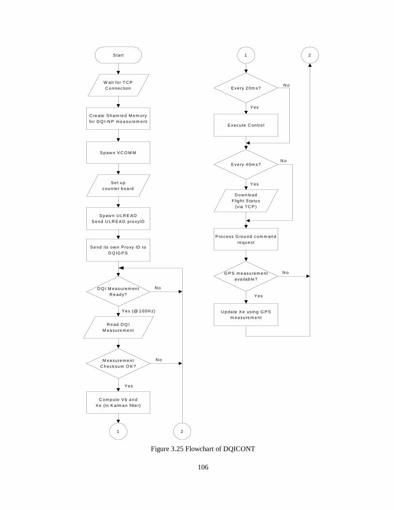
106

S tart

W ait for T C PC o nn ec tion

S p aw n V C O M M

Y es

N o

C re ate S h am re d M e m oryfo r D Q I-N P m e a su rem e nt

S e t u pcou nter b oa rd

S e nd its ow n P ro xy ID toD Q IG P S

D Q I M e asure m en tR e ad y?

Y es (@ 1 00 H z)

R e ad D Q IM ea sure m e nt

M ea sure m e ntC h ecksu m O K ?

N o

C o m p ute V b a n dX e (in K alm a n filte r)

1

1

D o wn lo adF lig ht S ta tu s

(v ia TC P )

P ro cess G rou nd com m an dre qu es t

G P S m e asu rem e nta va ilab le ?

U p da te X e us in g G P Sm ea sure m e nt

2

2

N o

Y es

E xecu te C on tro l

E ve ry 2 0m s?

Y es

N o

S p aw n U LR E A DS e nd U L R E A D pro xyID

E ve ry 4 0m s?

Y es

N o

Figure 3.25 Flowchart of DQICONT

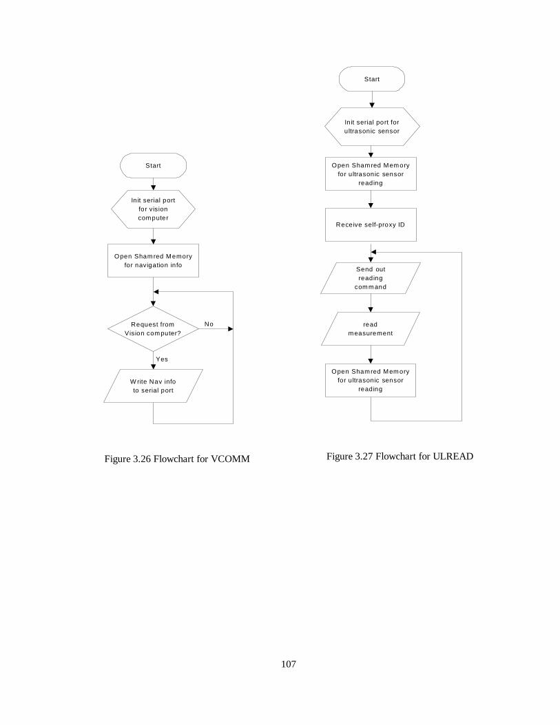
107

Start

Open Shamred Memoryfor navigation info

Request fromVision computer?

W rite Nav infoto serial port

No

Yes

Init serial portfor visioncomputer

Figure 3.26 Flowchart for VCOMM

Start

Open Shamred Memoryfor ultrasonic sensor

reading

readmeasurement

Send outreading

command

Open Shamred Memoryfor ultrasonic sensor

reading

Receive self-proxy ID

Init serial port forultrasonic sensor

Figure 3.27 Flowchart for ULREAD

108

DQ I-NP

M3512 3.12ms M3512 M3512

Yam aha R-50 RX signal

10 m s

21.78 ms

DQ ICONT

10 m s

PM W Signal Train

500 µs latencyfrom D ev.ser

Trigger IRQ 7

IRQ 7 Handler(T riggered by falling edge of PW M for th rottle )

IRQ latency (µ s)

Read PW Msignal

Return P roxy

RS-232Pu lse train

K alm anC o m pu te Vb Xe

50 µµ s

C on tro l50~10 0µµ s

1/2

D o w nloa d M 1101~200µµ s

1/4

P ro c essG r ou n d C o m m an d

100 µµ sS en d RX V alue

100µµ s~1/2

S en d Us e ns o rV alu e100 ~2 00µµ s

~1/7

Process time:200-400 µs, 1ms max

DQ ICONT Nom inal Execution Time (P233)

C o m pu te Xem50 µµ s1/1 2.5

P ro c ess G PS100 ~1 50 µµ s

1/1 2,5

200 ~400 µµ s , 1 m s m ax im u m

Figure 3.28 Real-time performance of onboard flight control software

109

Chapter 4

4. Hierarchical Flight Control System

Synthesis

In this part of the research, we aim to construct a controller architecture that conforms to the

hierarchical structure presented in Figure 1.3. The idea of the architecture is to build a hierarchical

multiple-layer structure that decomposes the abstract mission objectives into physical quantities of

control input. At the highest level, is the strategic planner, which determines the desired motion of the

RUAV for a finite horizon based on the mission objective and the current navigation status. In the

middle of the hierarchy, an intermediate layer interprets the output of the strategic planner and

chooses the current flight mode and the associated reference trajectory in realtime. In the lower part,

the regulation layer reads the realtime reference trajectory and issues the feedforward/feedback

control output for the helicopter airframe in realtime. At the lowest level is the physical helicopter

system. The helicopter responds to the control input from the regulation layer and the vehicle

response is measured by the navigation sensors and fed back to the regulation layer and the waypoint

navigator. The waypoint navigator monitors the navigation and the vehicle status to determine if the

current flight mode is being realized correctly or if there is some fault or exogenous disturbance in the

system. Based on the waypoint navigator’s decision, the given task is carried on or aborted.

In Figure 4.1, the hierarchical structure that has been developed for our RUAV application is

presented, As can be noticed, the proposed structure is slightly differently structure than the original

structure shown in Figure 1.3. The major difference is that the tactical planner and the trajectory

generator in Figure 1.3 are combined into a single layer. The reason for this modification is that the

110

reference trajectory is completely dependent on the current flight mode and it is more reasonable to

generate both the trajectory and the flight mode in a single module.

In this research, the lower two layers, the waypoint navigator and the regulation layer, are

mainly developed while maintaining compatibili ty with the hierarchical structure. The waypoint

navigator receives the motion command from the strategic planner and determines the appropriate

flight mode and the associated reference trajectory. The waypoint navigator activates the proper

control sets and sends the reference trajectory data in real time. In order to integrate these two layers

with the strategic planner, a methodology to convey the necessary information independent of the

mission and specific vehicle type is desired. To address this abstraction, the novel concept of Vehicle

Control Language (VCL) is developed. VCL is a script-type human understandable language that

encapsulates the flight mode, waypoint coordinates and other optional specifiers. Through the use of

VCL, the autopilot system becomes independent of the detail of the mission. As a direct consequence,

a more versatile flight control system can be implemented. These two major tasks of building the

regulation layer and the waypoint navigator are discussed in this chapter. In accordance with the

consistently used bottom-up approach, we first develop the stabili zing feedback control systems for

hover. These systems are fully tested in a series of the test flights. In the next step, the waypoint

navigator is developed using the framework of the VCL.

Vehicle DynamicsNavigation

Sensors

Strategy Planner

Flight modeReference Trajectory

Feedforward/Feedback control

ControlInput

Communication Channel

Command Status

W aypointsConflictnotification

TrackingError

W aypointNavigator

Figure 4.1 Modified hierarchical vehicle control system

111

4.1 Regulation Layer The helicopter has inherently unstable, complicated, and nonlinear dynamics under the significant

influence of exogenous disturbances and parameter perturbations. The system has to be stabili zed by

using a feedback controller. The stabili zing controller may be designed by the model-based

mathematical approach or by heuristic control algorithms. Due to the complexity of the helicopter

dynamics, there have been efforts to apply non-model-based approaches such as fuzzy-logic control,

neural network control, or a combination of these [6]. While these approaches are attractive because

no identification is required, they do not guarantee closed-loop stabili ty while they are being tuned or

being learning. The mathematical model-based approach assumes the availabili ty of a linear or

nonlinear system model for the controller design. In this case, the system identification process takes

the significant amount out of the whole research effort of building a RUAV. As our goal is to provide

a feedback controller that is consistently reliable, we seek a suboptimal controller using the model-

base approach. In the early part of the Berkeley UAV research, three different approaches were

chosen: (1) linear robust control using -synthesis, (2) feedback linearization, and (3) genetic fuzzy

approach [6]. All of these controllers showed satisfactory stabili zation and tracking performance

when working with the nominal plant with acceptable level although certain differences are observed

with plant perturbation and/or exogenous disturbance are introduced. While the genetic-fuzzy logic

and the -synthesis control showed robustness to those adversary effects, the performance of the

feedback linearization controller degraded considerably with the increased uncertainty and the

external disturbance. In fact, the feedback linearization control theory can be applied, as for now, to

very limited class of simple nonlinear systems. In efforts to cast the realistic nonlinear model into

such a framework, extreme simplification and misleading assumptions have been introduced in many

previous works. The resulting control law obtained by this approach would not be able to perform as

promised by the simulation when in the presence of the neglected dynamics, model perturbations, or

sensor noise.

The linear control theory has drawbacks of its own. First of all, the helicopter model is not

linear by any means. The dynamics feature strongly nonlinear effects and the equations of motion are

governed by the nonlinear kinematic relationship. Nonetheless, it has been proved that linear control

theory is able to stabili ze unstable nonlinear dynamics consistently, as long as the system stays in the

region where the linearity assumption holds. The deficiency of the linear approach in the coordinate

transformation should be taken care of by a separate algorithm. For example, the linear controller

does not understand the heading other than 0°. The forward flight with a fixed heading of other than

0° is realized only through an explicit coordinate transformation of the tangent plane position

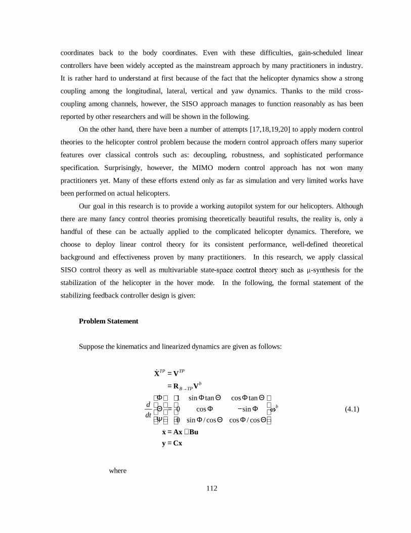
112

coordinates back to the body coordinates. Even with these difficulties, gain-scheduled linear

controllers have been widely accepted as the mainstream approach by many practitioners in industry.

It is rather hard to understand at first because of the fact that the helicopter dynamics show a strong

coupling among the longitudinal, lateral, vertical and yaw dynamics. Thanks to the mild cross-

coupling among channels, however, the SISO approach manages to function reasonably as has been

reported by other researchers and will be shown in the following.

On the other hand, there have been a number of attempts [17,18,19,20] to apply modern control

theories to the helicopter control problem because the modern control approach offers many superior

features over classical controls such as: decoupling, robustness, and sophisticated performance

specification. Surprisingly, however, the MIMO modern control approach has not won many

practitioners yet. Many of these efforts extend only as far as simulation and very limited works have

been performed on actual helicopters.

Our goal in this research is to provide a working autopilot system for our helicopters. Although

there are many fancy control theories promising theoretically beautiful results, the reality is, only a

handful of these can be actually applied to the complicated helicopter dynamics. Therefore, we

choose to deploy linear control theory for its consistent performance, well-defined theoretical

background and effectiveness proven by many practitioners. In this research, we apply classical

SISO control theory as well as multivariable state-VSDFH FRQWURO WKHRU\ VXFK DV -synthesis for the

stabili zation of the helicopter in the hover mode. In the following, the formal statement of the

stabili zing feedback controller design is given:

Problem Statement

Suppose the kinematics and linearized dynamics are given as follows:

1 sin tan cos tan

0 cos sin

0 sin / cos cos / cos

TP TP

bB TP

bd

dt

→

=

=Φ Φ Θ Φ Θ

Θ = Φ − Φ Ψ Φ Θ Φ Θ

= +=

X V

R V

&

x Ax Bu

y Cx

(4.1)

where

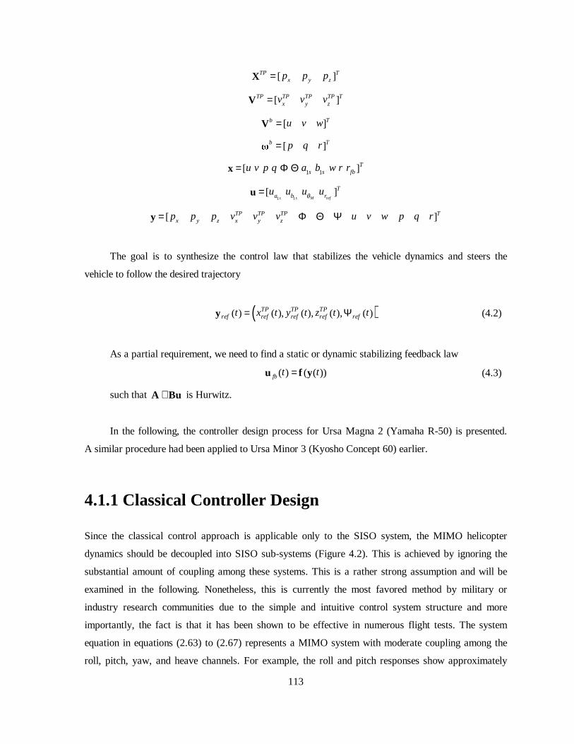
113

1 1

1 1

[ ]

[ ]

[ ]

[ ]

[ ]

[ ]

[ ]

s s M ref

TP Tx y z

TP TP TP TP Tx y z

b T

b T

Ts s fb

Ta b r

TP TP TP Tx y z x y z

p p p

v v v

u v w

p q r

u v p q a b w r r

u u u u

p p p v v v u v w p q r

θ

=

=

=

=

= Φ Θ

=

= Φ Θ Ψ

X

V

V

&

x

u

y

The goal is to synthesize the control law that stabili zes the vehicle dynamics and steers the

vehicle to follow the desired trajectory

( )( ) ( ), ( ), ( ), ( )TP TP TPref ref ref ref reft x t y t z t t= Ψy (4.2)

As a partial requirement, we need to find a static or dynamic stabili zing feedback law

( ) ( ( ))fb t t=u f y (4.3)

such that +A Bu is Hurwitz.

In the following, the controller design process for Ursa Magna 2 (Yamaha R-50) is presented.

A similar procedure had been applied to Ursa Minor 3 (Kyosho Concept 60) earlier.

4.1.1 Classical Controller Design

Since the classical control approach is applicable only to the SISO system, the MIMO helicopter

dynamics should be decoupled into SISO sub-systems (Figure 4.2). This is achieved by ignoring the

substantial amount of coupling among these systems. This is a rather strong assumption and will be

examined in the following. Nonetheless, this is currently the most favored method by mili tary or

industry research communities due to the simple and intuitive control system structure and more

importantly, the fact is that it has been shown to be effective in numerous flight tests. The system

equation in equations (2.63) to (2.67) represents a MIMO system with moderate coupling among the

roll, pitch, yaw, and heave channels. For example, the roll and pitch responses show approximately

114

15-25% coupling and the vertical mode agitates the yaw model due to the persistently varying anti-

torque of main rotor. Nonetheless, the system can be considered to be four sub-systems that consist of

roll~ yv , pitch~ xv , yaw and heave channels and each can be stabili zed by proportional-differential

(PD) controllers as will be discussed in the following. The roll and pitch rate dynamics show lightly

damped stable responses, which are similar to each other due to the symmetry of the main rotor

system. The roll and pitch angle dynamics can be seen as the cascade of integration and the attitude

rate dynamics, resulting in marginally stable systems. The feedback scheme to stabili ze the

longitudinal/lateral dynamics can be conceived by studying the root loci of those as shown later in

this section. Stepping one step out to the translational velocity dynamics, the dynamics from the

roll/pitch control input to xv and yv are clearly unstable as shown in Section 2.2.8 and they cannot be

stabili zed with proportional feedback of the translational velocity only in each channel. The vertical

and yaw dynamics have a strongly coupled nature due to the anti-torque of the main rotor. The

inherent dynamics of these channels are stable because of the aerodynamic relationship with the lift

and the local inflow. However, further damping of the vertical dynamics is desired because of the

sluggish response of the Yamaha R-50. The yaw dynamics is already damped sufficiently by the

built-in rate gyroscope system. In this case, assuming the gyro system is tuned properly, only the

angle regulation is required.

Rol l~Vy

Pitch~Vx

1

s

1

s

Heave

Yaw

1

s

1

s

1au

1bu

Muθ

Tuθ

byv

b

xv

r

ˆ yp

ˆ xp

ˆ zp

Ψ

Rate gyro

Yaw feedbackMixer

refru

bzv

Servo

Servo

Servo

Servo

Figure 4.2 SISO representation of helicopter dynamics

115

Based on these observations, the control law by the classical SISO approach is established as

shown in (4.4). The control law is very simple and static. Currently it does not involve any dynamic

controllers yet because the static control achieves a reasonable performance and the measurements for

feedback do not require any further filtering.

1

1

y y

x x

M z z

ref

a v p p

b u p p

w p p

r

u K K v K

u K K u K

u K w K

u K

θ

Φ

Θ

Ψ Ψ

= − Φ − − ∆

= − Θ − − ∆

= − − ∆

= − ∆

(4.4)

• Attitude Control

The attitude dynamics indicates the behavior when the translational motion in x and y direction

is constrained. For the design of attitude feedback design, we extract the attitude dynamic model by

fixi ng the state variables of translational velocities in x, y, and z-direction and the yaw terms to zero.

The eigenvalues of the attitude dynamics of the Ursa Magna 2 are 0, 0, -1.5729±12.2576i (roll)

and -1.8706± 8.2616i (pitch). The poles at the origin yield marginal stabili ty. The root-locus suggests

that the attitude dynamics may be stabili zed by simple attitude feedback only. The proper gains for

the roll and pitch loop can be found by the root loci and the step responses with various gains and

they are chosen to be 0.55, 0.55K KΦ Θ= − = .

With the stabili zation of the attitude dynamics, it should be noted that we could design a more

sophisticated control law involving filters. The structure of the proposed controller has a close

relationship with the characteristics of the employed navigation sensors. As commented earlier, the

Boeing DQI-NP INS produces attitude estimates with a relatively low bandwidth. Therefore, we do

not need to filter high frequency noise for our control problem and the attitude estimates may be

directly used for control law computation. We also intentionally avoided introducing angular rate

feedback for further modification of the underlying attitude dynamics because the angular rate

measurements contain a large portion of noise due to the severe structural vibration of the helicopter.

In addition, simpler control laws were preferred in the early stages of the controller experiments. The

proposed control laws of proportional gains perform reasonably.

116

−3 −2.5 −2 −1.5 −1 −0.5 0 0.5 1−15

−10

−5

0

5

10

15

Real Axis

Imag

Axi

s

root locus for roll mode

Kr= −0.55

Time (sec.)

Am

plitu

de

Step Response

0 1 2 3 4 5 6 7 8 9 10−3.5

−3

−2.5

−2

−1.5

−1

−0.5

0From: U(1)

To:

Y(1

)

−0.3

−0.4

−0.5

Kr= −0.55

−0.6

−3 −2.5 −2 −1.5 −1 −0.5 0 0.5 1 1.5 2−15

−10

−5

0

5

10

15

Real Axis

Imag

Axi

s

root locus for pitch mode

Time (sec.)

Am

plitu

de

Step Response

0 1 2 3 4 5 6 7 8 9 10−80

−70

−60

−50

−40

−30

−20

−10

0From: U(1)

To:

Y(1

)

−0.01

−0.015

kvy= −0.02

−0.03

Figure 4.3 Attitude Compensator Design

• Horizontal Velocity Control

Once the attitude sub-dynamics are stabili zed, we proceed to find the stabili zing feedback gains

for the velocity dynamics with the similar approach. Based on the root loci and step responses of the

velocity dynamics as shown in Figure 4.4, we find the suitable gains to be: 0.02, 0.02u vK K= − = − .

The gains in the roll and pitch loops are identical so far due to the very similar dynamic

characteristics of these channels. It is expected, if we recall that the roll dynamics has a faster

response, that the roll channel will show a faster response than the pitch channel.

With the combined use of proportional feedback for the attitude and the velocity, we could

stabili ze the longitudinal-lateral dynamics. The proposed controller structure is extremely simple but,

as proved in the experiment, very effective in stabili zing the targeted dynamics. The closed-loop

dynamics become fully stable so that the manual control in this presence of the stabili zing feedback

control becomes very stable and easy.

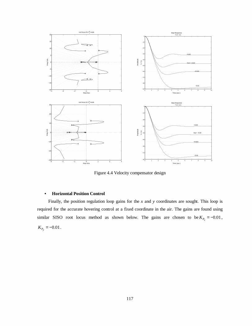
117

−4 −3 −2 −1 0 1 2−20

−15

−10

−5

0

5

10

15

20

Real Axis

Imag

Axi

s

root locus for Vbx mode

Time (sec.)

Am

plitu

de

Step Response

0 1 2 3 4 5 6 7 8 9 10−90

−80

−70

−60

−50

−40

−30

−20

−10

0From: U(1)

To:

Y(1

)

−0.01

−0.015

kvx= −0.02

−0.03

−3 −2 −1 0 1 2 3−30

−20

−10

0

10

20

30

Real Axis

Imag

Axi

s

root locus for Vby mode

Time (sec.)

Am

plitu

de

Step Response

0 1 2 3 4 5 6 7 8 9 10−80

−70

−60

−50

−40

−30

−20

−10

0From: U(1)

To:

Y(1

)

−0.01

−0.015

kvy= −0.02

−0.03

Figure 4.4 Velocity compensator design

• Horizontal Position Control

Finally, the position regulation loop gains for the x and y coordinates are sought. This loop is

required for the accurate hovering control at a fixed coordinate in the air. The gains are found using

similar SISO root locus method as shown below. The gains are chosen to be 0.01xPK = − ,

0.01yPK = − .

118

−2 −1.5 −1 −0.5 0 0.5 1−15

−10

−5

0

5

10

15

Real Axis

Imag

Axi

s

root locus for Pbx mode

Time (sec.)

Am

plitu

de

Step Response

0 1 2 3 4 5 6 7 8 9 10−140

−120

−100

−80

−60

−40

−20

0From: U(1)

To:

Y(1

)

kpx= −0.01

−0.0077

−0.015

−0.02

−2 −1.5 −1 −0.5 0 0.5 1−15

−10

−5

0

5

10

15

Real Axis

Imag

Axi

s

root locus for Pby mode

Time (sec.)

Am

plitu

de

Step Response

0 1 2 3 4 5 6 7 8 9 10−140

−120

−100

−80

−60

−40

−20

0From: U(1)

To:

Y(1

)

−0.008

kpy=−0.01

−0.015

−0.02

Figure 4.5 Position compensator design

• Heave and Yaw Control

We can proceed in a similar way to design the compensators for the heave and yaw dynamics.

It should be noted that the heave dynamics is inherently stable due to the aerodynamics of lift

generation. Still , introducing further damping by velocity feedback improves the system response

considerably. The altitude control can be realized by proportional altitude error feedback. The heave

control loop has the architecture of typical motion control because of the base dynamics. The control

loop consists of velocity feedback for further stabili zation and the altitude deviation feedback. The

gains are chosen to be 0.035zVK = and 0.12

zPK =

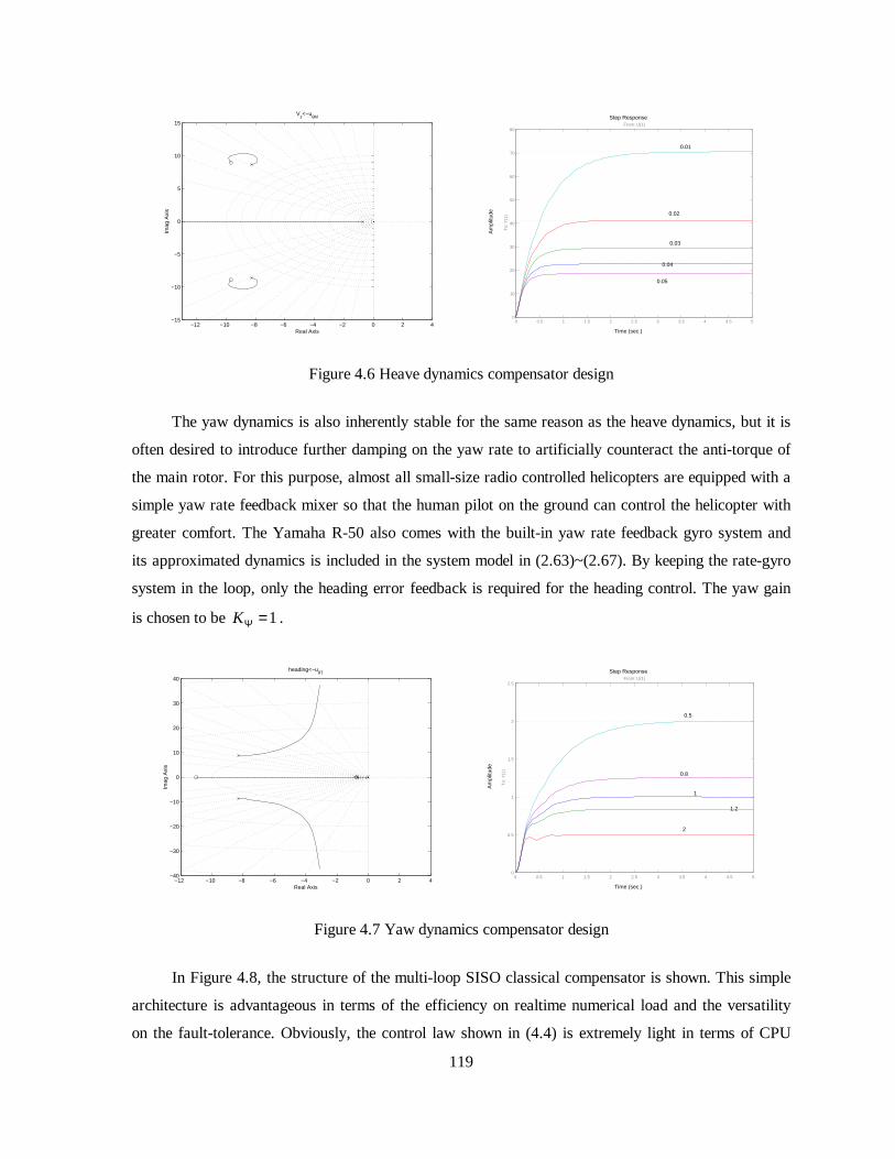
119

−12 −10 −8 −6 −4 −2 0 2 4−15

−10

−5

0

5

10

15

Real Axis

Imag

Axi

s

Vz<−uθM

Time (sec.)

Am

plitu

de

Step Response

0 0.5 1 1.5 2 2.5 3 3.5 4 4.5 50

10

20

30

40

50

60

70

80From: U(1)

To:

Y(1

)

0.05

0.04

0.03

0.02

0.01

Figure 4.6 Heave dynamics compensator design

The yaw dynamics is also inherently stable for the same reason as the heave dynamics, but it is

often desired to introduce further damping on the yaw rate to artificially counteract the anti-torque of

the main rotor. For this purpose, almost all small-size radio controlled helicopters are equipped with a

simple yaw rate feedback mixer so that the human pilot on the ground can control the helicopter with

greater comfort. The Yamaha R-50 also comes with the built-in yaw rate feedback gyro system and

its approximated dynamics is included in the system model in (2.63)~(2.67). By keeping the rate-gyro

system in the loop, only the heading error feedback is required for the heading control. The yaw gain

is chosen to be 1KΨ = .

−12 −10 −8 −6 −4 −2 0 2 4−40

−30

−20

−10

0

10

20

30

40

Real Axis

Imag

Axi

s

heading<−uθT

Time (sec.)

Am

plitu

de

Step Response

0 0.5 1 1.5 2 2.5 3 3.5 4 4.5 50

0.5

1

1.5

2

2.5From: U(1)

To:

Y(1

)

0.5

0.8

1

1.2

2

Figure 4.7 Yaw dynamics compensator design

In Figure 4.8, the structure of the multi-loop SISO classical compensator is shown. This simple

architecture is advantageous in terms of the efficiency on realtime numerical load and the versatili ty

on the fault-tolerance. Obviously, the control law shown in (4.4) is extremely light in terms of CPU

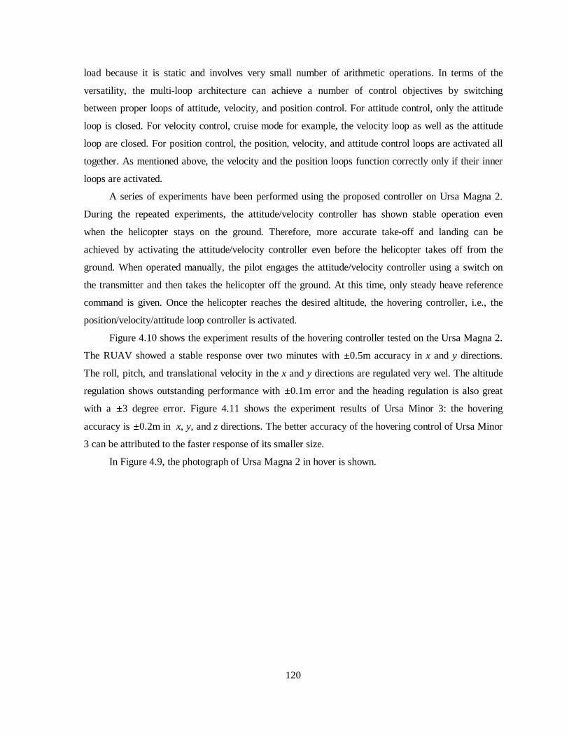
120

load because it is static and involves very small number of arithmetic operations. In terms of the

versatili ty, the multi-loop architecture can achieve a number of control objectives by switching

between proper loops of attitude, velocity, and position control. For attitude control, only the attitude

loop is closed. For velocity control, cruise mode for example, the velocity loop as well as the attitude

loop are closed. For position control, the position, velocity, and attitude control loops are activated all

together. As mentioned above, the velocity and the position loops function correctly only if their inner

loops are activated.

A series of experiments have been performed using the proposed controller on Ursa Magna 2.

During the repeated experiments, the attitude/velocity controller has shown stable operation even

when the helicopter stays on the ground. Therefore, more accurate take-off and landing can be

achieved by activating the attitude/velocity controller even before the helicopter takes off f rom the

ground. When operated manually, the pilot engages the attitude/velocity controller using a switch on

the transmitter and then takes the helicopter off the ground. At this time, only steady heave reference

command is given. Once the helicopter reaches the desired altitude, the hovering controller, i.e., the

position/velocity/attitude loop controller is activated.

Figure 4.10 shows the experiment results of the hovering controller tested on the Ursa Magna 2.

The RUAV showed a stable response over two minutes with 0.5m accuracy in x and y directions.

The roll, pitch, and translational velocity in the x and y directions are regulated very wel. The altitude

regulation shows outstanding performance with 0.1m error and the heading regulation is also great

with a 3 degree error. Figure 4.11 shows the experiment results of Ursa Minor 3: the hovering

accuracy is 0.2m in x, y, and z directions. The better accuracy of the hovering control of Ursa Minor

3 can be attributed to the faster response of its smaller size.

In Figure 4.9, the photograph of Ursa Magna 2 in hover is shown.

121

Figure 4.8 The architecture of proposed SISO multi-loop controllers

Figure 4.9 Ursa Magna 2 in automatic hover

122

46.5 47 47.5−52.4

−52.2

−52

−51.8

−51.6

−51.4

x [m]

y [m

]

0 10 20 30 40 5046.6

46.8

47

47.2

47.4

time [sec]

x [m

]

0 10 20 30 40 50−52.6

−52.4

−52.2

−52

−51.8

−51.6

−51.4

−51.2

time [sec]

y [m

]

0 10 20 30 40 501.05

1.1

1.15

1.2

1.25

1.3

time [sec]

−z

[m]

0 10 20 30 40 50−0.5

0

0.5

Vxb [m

/s]

0 10 20 30 40 50−5

0

5

Θ [d

eg]

0 10 20 30 40 50−20

0

20

q [d

eg/s

]

0 10 20 30 40 50−0.1

0

0.1

u B1 [m

s]

time [sec]

0 10 20 30 40 50−0.5

0

0.5

Vyb [m

/s]

0 10 20 30 40 50−5

0

5

Φ [d

eg]

0 10 20 30 40 50−50

0

50

p [d

eg/s

]

0 10 20 30 40 50−0.05

0

0.05

u A1 [m

s]

time [sec]

Figure 4.10 Experiment result of autonomous hovering of Ursa Magna 2

123

0 10 20 30 40 50−1.4

−1.2

−1

z [m

]

0 10 20 30 40 50−0.5

0

0.5

Vzb [m

/s]

0 10 20 30 40 50−0.1

0

0.1

u θ M

[ms]

0 10 20 30 40 50−90

−85

−80

Ψ [d

eg]

0 10 20 30 40 50−10

0

10

r [d

eg/s

]

0 10 20 30 40 50−0.1

0

0.1

u θ T

[ms]

Figure 4.10 (‘cont)

0 20 40 60 8014.1

14.2

14.3

14.4

14.5

14.6

X [m

]

time [sec]0 20 40 60 80

−1.7

−1.6

−1.5

−1.4

−1.3

Y [m

]

time [sec]

0 20 40 60 800.6

0.7

0.8

0.9

1

−Z

[m]

time [sec]14.1 14.2 14.3 14.4 14.5 14.6

−1.7

−1.6

−1.5

−1.4

−1.3

X [m]

Y [m

]

Figure 4.11 Experiment results of autonomous hovering on Ursa Minor 3

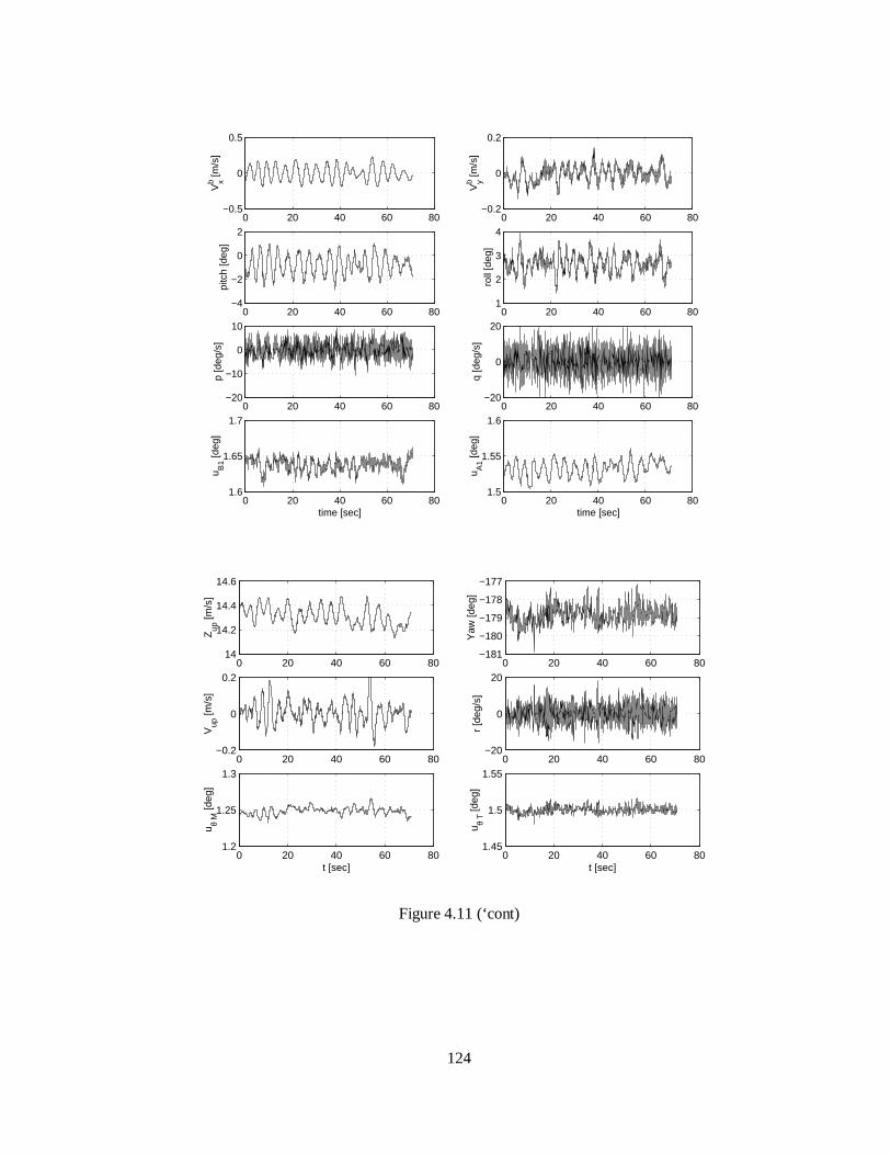
124

0 20 40 60 80−0.5

0

0.5

Vb x [m

/s]

0 20 40 60 80−0.2

0

0.2

Vb y [m

/s]

0 20 40 60 80−4

−2

0

2pi

tch

[deg

]

0 20 40 60 801

2

3

4

roll

[deg

]

0 20 40 60 80−20

−10

0

10

p [d

eg/s

]

0 20 40 60 80−20

0

20

q [d

eg/s

]

0 20 40 60 801.6

1.65

1.7

u B1 [d

eg]

time [sec]0 20 40 60 80

1.5

1.55

1.6

u A1 [d

eg]

time [sec]

0 20 40 60 8014

14.2

14.4

14.6

Zup

[m/s

]

0 20 40 60 80−0.2

0

0.2

Vup

[m/s

]

0 20 40 60 80−181

−180

−179

−178

−177

Yaw

[deg

]

0 20 40 60 80−20

0

20

r [d

eg/s

]

0 20 40 60 801.2

1.25

1.3

u θ M

[deg

]

t [sec]0 20 40 60 80

1.45

1.5

1.55

u θ T [d

eg]

t [sec]

Figure 4.11 (‘cont)

125

Figure 4.12 Ursa Minor 3 in autonomous hover above the ship deck simulator

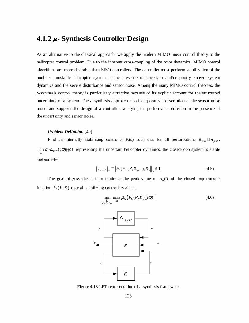
126

4.1.2 - Synthesis Controller Design

As an alternative to the classical approach, we apply the modern MIMO linear control theory to the

helicopter control problem. Due to the inherent cross-coupling of the rotor dynamics, MIMO control

algorithms are more desirable than SISO controllers. The controller must perform stabili zation of the

nonlinear unstable helicopter system in the presence of uncertain and/or poorly known system

dynamics and the severe disturbance and sensor noise. Among the many MIMO control theories, the

-synthesis control theory is particularly attractive because of its explicit account for the structured

uncertainty of a system. The -synthesis approach also incorporates a description of the sensor noise

model and supports the design of a controller satisfying the performance criterion in the presence of

the uncertainty and sensor noise.

Problem Definition [49]

Find an internally stabili zing controller K(s) such that for all perturbations pert pert∆ ∈û ,

( )max 1pert jω

ωσ ∆ ≤ representing the uncertain helicopter dynamics, the closed-loop system is stable

and satisfies

[ ( , ), ] 1e d L U pertT F F P K← ∞ ∞= ∆ ≤ (4.5)

The goal of -synthesis is to minimize the peak value of ( )µ∆ ⋅ of the closed-loop transfer

function ( , )LF P K over all stabili zing controllers K i.e.,

( )min max ( , )( )stabilizing

LK

F P K jω

µ ω∆ (4.6)

P

K

per t∆

z w

d

uy

e

Figure 4.13 LFT representation of -synthesis framework

127

P is the generalized plant, which includes the helicopter linear model and weighting matrix

blocks for the sensor noise model and the performance specifications. The structure of the generalized

plant should be carefully designed so that the resulting controller K may fulfill all of the robust

stabili ty and robust performance requirements. The generalized plant contains the helicopter

dynamics, uncertainty weighting, noise weighting, reference response model and performance

weighting. The attitude dynamics is extracted from equation (2.63) by discarding the state variables u,

v, w, r, and fbr , as shown in the following:

att att att att att

att att att

= +=

x A x B u

y C x

(4.7)

where

1 1[ ]Tatt s sp q a b= Φ Θx (4.8)

1 1

[ ]s s

Tatt a bu u=u (4.9)

[ ]Tatt p q= Φ Θy (4.10)

1 1

1 1

1

1

1 1

1 1

0 0 0 0

0 0 0 0

1 0 0 0 0 0

0 1 0 0 0 0

0 1 0 0 1/

1 0 0 0 1/

0 0

0 0

0 0

0 0

s s

s s

s

s

a s b s

a s b s

a b

a b

att

f b

a f

att

u u

u u

L L

M M

A

B

A A

B B

τ

τ

= − − − − =

A

B

(4.11)

As discussed above, the helicopter dynamics, when the translational dynamics is constrained,

are marginally stable. In the -synthesis framework, the interconnection for the generalized plant P

and the weighting functions are the design parameters. The interconnection diagram is given in Figure

4.15, which includes a number of weighting functions categorized as (1) uncertainty model, (2) noise

model, (3) control input penalty model, (4) handling quality model, (5) performance weighting model.

128

Frequency (rad/sec)

Sin

gula

r V

alue

s (d

B)

Singular Values

10−4

10−3

10−2

10−1

100

101

102

−40

−20

0

20

40

60

80

Figure 4.14 Singular value plot of the attitude dynamics of Ursa Magna

HelicopterAttitude

Dynamics

+

+

WU

WN

+

+

+

+

WP2

+

+

WP1

WQ -

-

dΦ

dΘ

Φ

Θ

p

q

1au

1bu

WA

∆

n(1:4)

1(1: 2)Pe

2(1: 2)Pe

(1: 2)Ae

K

Figure 4.15 Interconnection diagram for -synthesis controller design

129

The weighting functions specify the characteristics of the controller under the framework of the

minimization of the closed-loop system input-output infinity norm as shown in (4.5). Roughly

speaking, the weighting functions shape the controller so that the input-output ratio is smaller than

1.For example, if a weighting function penalize the deviation of the system response from the model

response by 10, the error of the closed-loop system would be around 10%. The actual behavior of the

-synthesis controller is significantly more complicated than this simplified interpretation.

• Uncertainty Model

The uncertainty or unmodeled dynamics of the helicopter system equation may be categorized

as: 1) poorly identified or time-varying aerodynamics or inertial quantities, 2) unmodeled higher

order dynamics such as the rotor flapping dynamics or the servomotor dynamics and 3) nonlinear

effects of the kinematic and dynamic system equations. All of these may perturb the resulting closed-

loop linear control systems out of stable region, so the controller should be designed to be robust to

those effects. The uncertainty model associated with the helicopter dynamics is usually very hard to

establish due to the nonlinear complex behavior of the original helicopter dynamics. Therefore, 10 %

of the multiplicative input uncertainty in each channel is assumed as the starting point.

2 2

10.1

/10 1U

sW

s ×+=

+I (4.12)

10−2

10−1

100

101

102

103

0.1

0.2

0.3

0.4

0.5

0.6

0.7

0.8

0.9

1

Uncertainty Weighting Wu

Figure 4.16 Unstructured input uncertainty model

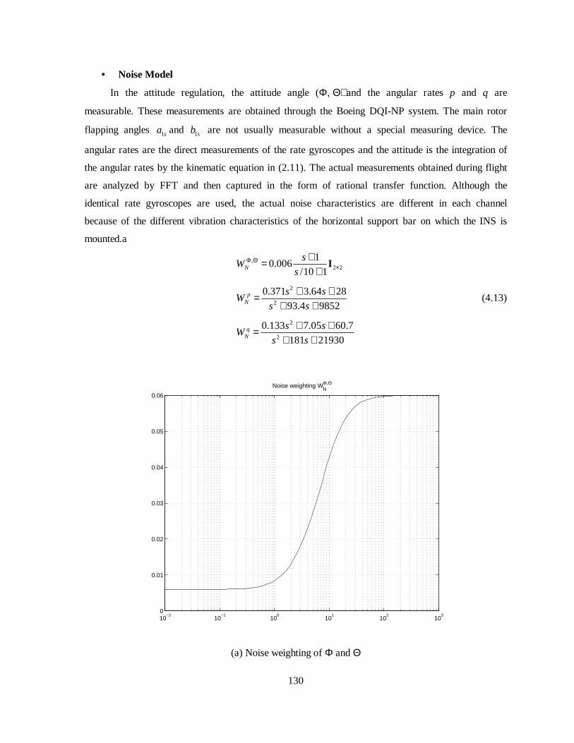
130

• Noise Model

In the attitude regulation, the attitude angle (Φ, Θ) and the angular rates p and q are

measurable. These measurements are obtained through the Boeing DQI-NP system. The main rotor

flapping angles 1sa and 1sb are not usually measurable without a special measuring device. The

angular rates are the direct measurements of the rate gyroscopes and the attitude is the integration of

the angular rates by the kinematic equation in (2.11). The actual measurements obtained during flight

are analyzed by FFT and then captured in the form of rational transfer function. Although the

identical rate gyroscopes are used, the actual noise characteristics are different in each channel

because of the different vibration characteristics of the horizontal support bar on which the INS is

mounted.a

,2 2

2

2

2

2

10.006

/10 1

0.371 3.64 28

93.4 9852

0.133 7.05 60.7

181 21930

N

pN

qN

sW

s

s sW

s s

s sW

s s

Φ Θ×

+=+

+ +=+ +

+ +=+ +

I

(4.13)

10−2

10−1

100

101

102

103

0

0.01

0.02

0.03

0.04

0.05

0.06

Noise weighting WΦ,ΘN

(a) Noise weighting of Φ and Θ

131

10−2

10−1

100

101

102

103

0

0.05

0.1

0.15

0.2

0.25

0.3

0.35

0.4

0.45

Noise weighting Wp,qN

Wp

Wq

(b) Noise weighting of angular rates p and q

Figure 4.17 The Noise weighting functions

• Reference Model

The reference response model specifies the response profile of the roll and pitch angle to

follow. The deviation of the system response from the desired response is penalized by the

performance weighting model that will be discussed in the following. The response model can be

considered as the handling quality model, which is a concept widely used in the aerospace

community. In this research, it is described by 2nd order critically damped transfer function. During

the flight test, it was discovered that the weighting on the error has significant effect not only on the

response shape but also the overall stabili ty of the overall closed-loop system response. This

phenomenon attributes to the mismatch of the linear system model with the nonlinearity of the system

model.

2

2 22 2, 0.6

2n

Q nn n

Ws s

ω ω πω ω ×= =

+ +I (4.14)

• Performance Weighting

The performance weighting consists of two parts. One part penalizes the deviation of the

system response from the reference model to force the helicopter to follow the reference model. The

132

other part penalizes the angular rates so that the Corioli’s acceleration and the gyroscopic effects do

not become large enough to disturb the linearity regime.

1

22 2

120 0 /100 10 100 1

13

/0.2 1

P

P

sW

s

sW

s ×

+= +

+=

+I

(4.15)

• Actuator Weighting

The purpose of the actuator weighting is mainly to penalize the input to the helicopter in order

to prevent saturation. A second-order model is chosen to penalize the control action at higher than 20

rad/s.

2

2 22

93.25 966.5 774.3

33.51 784.7A

s sW

s s ×+ +=

+ +I (4.16)

Time (sec.)

Am

plitu

de

Step Response

0 1.4 2.8 4.2 5.6 70

0.1

0.2

0.3

0.4

0.5

0.6

0.7

0.8

0.9

1From: U(1)

To:

Y(1

)

Figure 4.18 The step response of the reference model

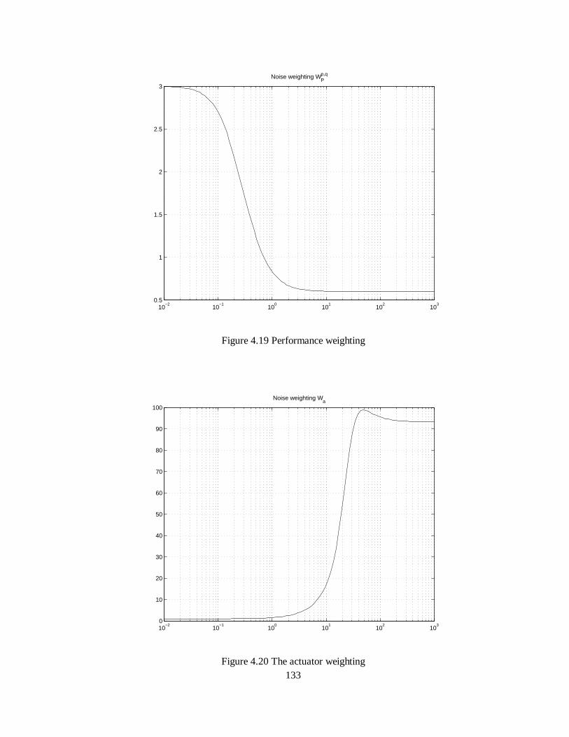
133

10−2

10−1

100

101

102

103

0.5

1

1.5

2

2.5

3

Noise weighting Wp,qP

Figure 4.19 Performance weighting

10−2

10−1

100

101

102

103

0

10

20

30

40

50

60

70

80

90

100

Noise weighting Wa

Figure 4.20 The actuator weighting

134

The controller K with 6 inputs and 2 outputs is computed using the algorithm known as D-K

iteration. The minimization problem in (4.6) is not easily solved with the operator of the structured

singular value µ. The P minimization problem is hence replaced with the minimization of the upper

bound of the P such that

( ) ( )1infD

M DMDµ σ −∆ ∈

≤ûD

(4.17)

During this iteration, it is aimed to find the controller K and the input-output scaling matrix D

in a alternating manner. At first, with D fixed, the controller K is sought by the ∞+ optimization

algorithm such that

min ( , )stabilizing

L DK

F P K ∞

Using the resulting K, the scaling matrix D such that

1min ( , )( )LDD F P K j D

ωω ωσ ω −

∈ D

is sought. This process is repeated by a reasonable number until any significant improvement of

the peak value of the P is made or the order of the controller reaches the limit of the reasonable size.

The D-K iteration is a heuristic algorithm that does not guarantee any convergence to the local

minima, not even the global minima of the minimization problem. Nonetheless, this algorithm yields

reasonable results most of the time. In Figure 4.21, the value of µ during the D-K iteration are shown.

The disadvantages of the P synthesis algorithm are (1) the effort to establish the interconnection

of the system and the individual weighting functions, (2) the tremendous off-line computation load,

(3) the on-line (realtime) computation load, and (4) the large size of the controller. The drawbacks (1)

and (2) are justified if the resulting performance of the P synthesis controller is superior to other

controllers. The drawback (3) as well as some part of (2) are not much of issues these days thanks to

the extremely fast and cheap computing capabili ty available even at PC level. The drawback (4) is

partially resolved by a number of order-reduction algorithms such as coprime factorization or Hankel-

norm minimization.

135

10−2

10−1

100

101

102

0

0.5

1

1.5

2

2.5

3

3.5

4µ bounds

1st

4th

2nd

3rd

Figure 4.21 µ bounds during the D-K iteration

The resulted controller K is 34th order and its singular value plot is given in Figure 4.22. As a

matter of fact, the large size of the resulted controller is one of the major drawback of the P synthesis

algorithm. In our application, the order of the controller has a direct impact on the realtime

computation time and the distortion of the controller by the truncation error of the real variables. In

terms of the realtime performance, the high order of the controller is not of too much concern any

more these days thanks to powerful but common CPUs. It was discovered that, after debugging, the

variable to hold the controller system matrix (A,B,C,D) should be declared as a double to keep the

perturbation of the poles by the truncation error to be minimal.

The resulted continuous-time controller is discretized with the bili near transform and

implemented on the FCS. As mentioned before, the execution time of the 34th order controller was

short enough to keep the 21.76 ms sampling time.

In Figure 4.23, the experimental results of the proposed -synthesis controller are given. It can

be verified that the controller is capable of stabili zing the helicopter system for sufficiently long time.

The graph shows that the roll angle is regulated within 2 degrees while pitch angle is within 3~4

degrees. It should be noted that the pitch angle could be more tightly controlled by using larger

penalty function WΘ .

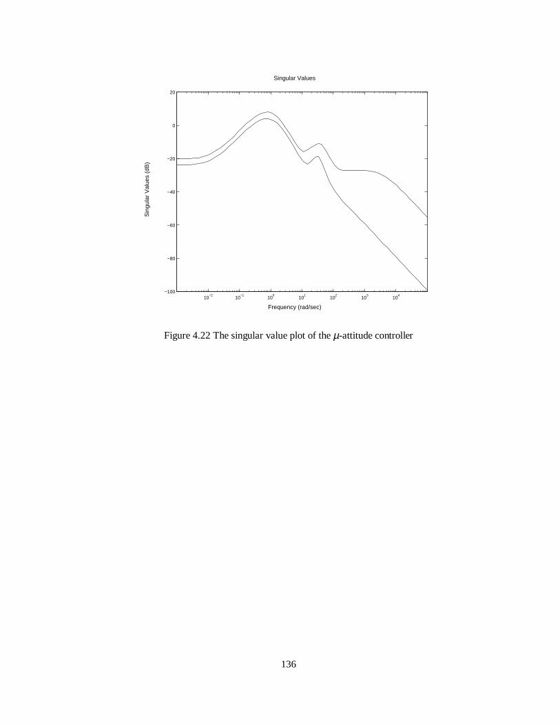
136

Frequency (rad/sec)

Sin

gula

r V

alue

s (d

B)

Singular Values

10−2

10−1

100

101

102

103

104

−100

−80

−60

−40

−20

0

20

Figure 4.22 The singular value plot of the µ-attitude controller

137

80 85 90 95 100 105 110−6

−4

−2

0

2

4

Rol

l, P

itch

[deg

]

80 85 90 95 100 105 110−0.1

−0.05

0

0.05

0.1

time [sec]

cont

rol i

nput

[ms]

280 285 290 295 300 305 310 315−0.1

−0.05

0

0.05

0.1

time [sec]

cont

rol i

nput

[ms]

280 285 290 295 300 305 310 315−8

−6

−4

−2

0

2

4

6

Rol

l, P

itch

[deg

]

Figure 4.23 Experiment results of attitude regulation by -synthesis controller

138

4.2 Waypoint Navigation In order for a RUAV to track the given flight paths with the regulation layer that was proposed in the

previous section, some supervising control logic should be synthesized for the hierarchical control

structure. This layer of supervising logic lies between the strategic planner and the regulation layer. It

receives the waypoint request from the strategic planner and reports the execution results of the given

request.

In the design of the waypoint navigator, the unique nature of the helicopter maneuverabili ty

should be taken into consideration. The flight modes of a RUAV can be categorized as (1) take-off,

(2) hover, (3) ascent, (4) descent, (5) forward flight, (6) bank-to-turn, (7) pirouette, and (8) land1. The

transition relationship among these flight modes is depicted as a state transition diagram in Figure

4.24. According to this diagram, a flight scenario of a RUAV can be understood as a sequential

combination of some of these modes. A mission of a helicopter starts with the Take-off mode, goes

through Hover and other flight modes, and ends with the Land mode. The Take-off and Land modes

are terminal nodes, which means that these modes are either starting or ending nodes. The other

modes are bi-directional, which means that the sequence can enter or exit this mode. Based on this

rule, a given mission scenario is decomposed into a sequence of flight modes either by the strategic

planner or by a human operator.

It is worthwhile to compare the flight characteristics of RUAV with that of FUAV. The flight

modes of conventional aircrafts can be categorized as (1) take-off, (2) climb, (3) cruise, (4) bank-to-

turn, (5) descent, and (6) land2. One important factor of any fixed-wing aircraft flight is that the

aircraft always has a positive forward velocity higher than the stall velocity. In contrast to the nature

of the fixed-wing aircraft, as can be understood from above, the RUAVs feature the superset of flight

modes. Whilst the FUAVs always have pass-by waypoints, the RUAVs may have pass-by waypoints

or stop-over waypoints. This versatili ty of the flight capability requires a more sophisticated waypoint

navigation algorithm.

Once the flight sequence is determined, the supervising logic of the waypoint navigator should

activate the correct combination of attitude/velocity/position control for the selected flight mode and

generate the associated reference trajectory. The output of the waypoint navigator is fed into the

1 More aggressive maneuvers or some combination of the listed flight modes are possible: the former include barrel-role, split-s, 540-degree stall turn and so on. The latter include forward take-off, cruise while climbing and so on. In this research, we limit our scope to the listed conventional flights. 2 Some type of f ixed-wing aircrafts, especially those with thrust-vectoring, can have very versatile flight characteristics. In this research, we will consider more conventional flight patterns.

139

regulation layer. We choose the multi-loop SISO controller proposed in Section 4.1.1 because of its

simple structure and acceptable performance that has been validated in a series of test flights.

Take-off Hover

Pirouette

Land Ascend/Descend

ForwardFlight

Low-speed

X-Y flight

Bank-to-turn

Figure 4.24 State transition diagram of helicopter control

In the following, the detailed definition of these modes are given:

• Take-off

Take-off mode is the starting point for all RUAV missions. In the beginning of this mode, the

helicopter rests still on the ground with engine on idle. The autopilot commands the aircraft to

reach the target altitude while the horizontal deviation is kept minimal. Once the aircraft reaches

the target altitude, it is ready to make transition to other possible flight modes. Here follows the

formal definition of the take-off mode:

0 0

0 0

0

0 0initial final

Hover

t t

X X

Y Y

Z Z

→ Ψ Ψ

(4.18)

140

where HoverZ is the target hover altitude

Apparently, a more aggressive way such as jump take-off is also possible. In this case, the

helicopter gains forward velocity as well as altitude simultaneously. This is in fact the

combination of the take-off mode and the forward flight according to our definition. In our study,

we exclude this mode for simplicity. Under this assumption, the first flight mode right after take-

off is enforced to be the hover mode.

• Hover

Hover indicates the state where the RUAV stays in the air with negligible speed and heading

change. This is the most essential flight mode to be accomplished by the autopilot system because

almost all flight patterns go through the hover mode. During this mode, the requirement given in

(4.19) should be satisfied.

From the view of the helicopter dynamics, the hover mode is considered as the state where the

influence of inflow on the rotor dynamics is negligible. Our own analysis shows that the influence

of the inflow is negligible up to 5 m/s in horizontal direction. Therefore, we may use the hover

controller for the control of low-speed forward flight, sideslip, pirouette and ascent/descent by

feeding in appropriate reference inputs to the appropriate channels.

( )max

( )max

( )max

( )max

ref tolt

ref tolt

ref tolt

ref tolt

X t X X

Y t Y Y

Z t Z Z

t

− ≤

− ≤

− ≤

Ψ − Ψ ≤ Ψ

(4.19)

initial, finalfor t [t t ]∀ ∈

• Landing

Landing is the opposite of the take-off mode in most aspects. This mode is entered from hover by

initiating a descent. At first, the autopilot system calculates the relative altitude, i.e., the relative

distance from the helicopter to the ground downright, using relative sensors such as the ultrasonic

altimeter or laser range finder and then generates the landing profile accordingly. The vehicle

descends slowly until i t touches the ground. The touchdown is detected securely by the four

ground contact switches mounted on the landing gear. Once the touchdown is detected, the

141

autopilot system reduces the engine RPM to idle and the main rotor collective pitch to zero. Then

the vehicle goes into the wait state until the mission is over or it resumes a new operation. The

definition of landing mode is given as:

0 0

0 0

0 0initial final

Hover Ground

t t

X X

Y Y

Z Z

→ Ψ Ψ

(4.20)

• Forward Flight

Forward flight is the state in which the helicopter gains and maintains nonzero forward velocity

while the heading is generally kept tangent to the flight path. This is the primary maneuver used

to visit the distant waypoints. This mode is divided into three phases: (1) acceleration, (2) cruise

with constant velocity, and (3) deceleration to stop if required. When the helicopter enters the

forward flight mode from hover, the forward velocity is controlled to follow certain profile while

the lateral velocity is regulated to zero. The forward velocity is attained by tilting the thrust of

main rotor slightly to forward direction through the longitudinal cyclic pitch control. Then the

vehicle starts accelerating in the forward direction. As the main rotor thrust is tilted forward by

the longitudinal cyclic pitch, the vertical component decreases, causing the vehicle to lose

altitude. To compensate this slight loss in the vertical thrust, the collective pitch would be

increased accordingly. In automatic control, the loss of the altitude should be compensated by the

separate altitude regulation loop. As the vehicle gains forward velocity, the inflow to the main

rotor and tail rotor affect the overall rotor dynamics. The rotor generates more lift, known as

translational li ft, due to the increased amount of the inflow in unit time. The relative airspeed

experienced by the blades becomes asymmetric and induces the flapping.

The forward flight can be categorized as (1) low-speed cruise and (2) high-speed cruise.

The determining factor between these two flights is the significance of the influence of the inflow

on main and tail rotors. The hover controller may be used if the effect of the local flow due to the

forward velocity is negligible. If the vehicle reaches a significant forward speed, the rotor

dynamics changes and the contributions of the fuselage, horizontal and vertical stabili zer fins

grow together. In this case, a separate controller optimized for the high-speed cruise dynamics

should be designed. As for now, we limit our scope to the low-speed forward flight, which can be

managed by the hover controller.

142

The reference trajectory for the forward motion may be generated using sophisticated

algorithms such as dynamics inversion. Detailed discussion will be given in the following section.

0 1

0 1

0 1

0 1finalinitial tt

X X

Y Y

Z Z

→ Ψ Ψ

(4.21)

while tracking

( ) ( )

max ( )

( ) ( )

( ) atan2( , )( ) ( )

ref

tolt

ref

TP TPy x refref

u t u t

vv t

w t w t

t V t V t

→

≤

→

Ψ →

(4.22)

• Low-speed flight

This maneuver indicates the low-speed flight in x-and/or y-direction. In this mode, the influence

of inflow on rotors, fuselage, and stabili zer fins are small enough to be ignored and hence the use

of hover control is justified. In this mode, the helicopter is controlled to have longitudinal as well

as lateral velocity to reach the target waypoint. The heading is maintained constant independent

from the direction of the flight path. The waypoint navigator generates the reference trajectory as

shown in (4.24). Although the rotor dynamics is symmetric because of the symmetric geometry of

rotor, the responses in the x and y directions are slightly different due to the asymmetric mass

moment of inertia in x and y axis. In the y-direction, the fuselage receives more wind drag and the

tail rotor dynamics is affected in a different manner.

0 1

0 1

0 1

0 0initial finalt t

X X

Y Y

Z Z

→ Ψ Ψ

(4.23)

while tracking

constant

( ) ( )

( ) ( )

( ) ( )

( )

ref

ref

ref

ref

u t u t

v t u t

w t w t

t

→

→

→

ΨΨ →

(4.24)

143

• Pirouette

Pirouette1 indicates a maneuver of changing the heading with minimal velocity deviation about

the main rotor axis. This mode is mainly controlled by the tail rotor collective pitch with

compensating inputs from other channels. The unbalanced lateral force of the tail rotor should be

canceled by the cyclic pitch of main rotor in roll direction. The engine RPM perturbation due to

the tail rotor pitch variation should be regulated by the engine governor.

max ( )

max ( )

max ( )

( ) ( )

tolt

tolt

tolt

ref

uu t

vv t

ww t

t t

≤

≤

≤

Ψ → Ψ

(4.25)

• Ascent/Descent

This flight mode indicates, in a narrow sense, the vertical motion while horizontal velocity and

the heading deviation are kept minimal. The vertical mode is dominantly controlled by the main

rotor collective pitch. During ascent, the rotor has to generate more lift by increasing the pitch.

This alone requires more power from the power plant. The vertical velocity of the helicopter

affects the lift generation of the rotor and imposes additional drag on the blade, which requires

more power. Therefore, the rate of ascent is limited by the maximum horsepower of the engine.

The behavior with the descent mode is more complicated than ascent. A low-rate descent is

achieved by slightly decreasing the main rotor collective pitch and, in turn, main rotor thrust.

When the helicopter descends faster to reach the same speed of the induced velocity of main

rotor, the blades are unable to push down air and cannot produce thrust any more. This dangerous

state is called vortex ring and it should be avoided because in this state the control over the

vehicle is simply lost. If the vehicle manages to pass this region quickly and descends faster, the

rotor enters the windmill state and it begins to receive power from the passing air. With the

proper collective pitch, the vehicle finds an equili brium in vertical descent and this state can be

sustained. This condition is called autorotation and it corresponds to the gliding of fixed-wing

aircrafts. In the case of engine malfunction, the pilot can disconnect the dead engine output shaft

with the main rotor shaft, let the main rotor enter the autorotation state, and safely land the

vehicle.

1 This French word originally means a full turn on the toe or ball of one foot in ballet. In this paper, the term “pirouette” is favored over “turn” because the latter word may be confusing to indicate “turn” about a fixed axis or “bank-to-turn” at higher forward velocity.

144

Although we do not need to be concerned too much with this advanced capabili ty of the rotorcraft

for now, the autopilot should be programmed to stay off f rom the unsafe ascent and descent rates.

These hard bounds dependent on the helicopter configuration should be considered to generate

the reference trajectory by the waypoint navigator.

Ascent and descent modes can be defined as following:

( )max

( )max

( )max

( ) ( )

( )

ref tolt

ref tolt

ref tolt

ref

ref

X t X X

Y t Y Y

t

w t w t

t

− ≤

− ≤

Ψ − Ψ ≤ Ψ

→Ψ → Ψ

(4.26)

In general, ascent or descent may occur while the vehicle has nonzero horizontal velocity or

turning rate. From the viewpoint of dynamics and control, the vertical mode is relatively less

coupled with horizontal mode so that the simultaneous control of horizontal and vertical velocity

may be achieved easily. During ascent or descent, the tail rotor collective pitch should be

controlled accordingly to counteract the change in the anti-torque of the main rotor, which is the

function of main rotor collective pitch or thrust.

4.2.1 Vehicle Control Language

Vehicle Control Language, or VCL, is a framework to describe the given mission with human-

understandable form of script language. VCL includes a set of commands to realize the flight modes

listed in Figure 4.24 so that a given mission can be described in a sequence of the achievable flight

modes. This approach provides the isolation and abstraction between the low-level vehicle control

and the mission-level condition. In this framework, the onboard autopilot system can perform any

given feasible mission without any reprogramming of the onboard software as the mission changes.

The sequence of motion commands is described in a script language form that is understandable to

humans.

A VCL command line consists of the command verb, required parameters and optional

parameters. VCL flight commands typically take the form:

145

command <target coordinates> options

• Command

This part of VCL script specifies the type of maneuver. Currently, TakeoffT o, Hover,

FlyTo, MoveTo and Land commands are defined. Among these Hover, FlyTo, and

MoveTo commands are implemented in VCL-based waypoint navigator and tested successfully

as will be shown in the following section.

• Target coordinates

This part specifies the target coordinate either in absolute coordinates or in relative coordinates in

the local Cartesian frame. The type of coordinates is specified by the postfix abs or rel. The

absolute coordinates are referred to the origin in the test field as defined in Figure C.1 in

Appendix. The relative coordinates specify the difference from the last target point specified by

the previous line of VCL. If no previous value is set, the current position is taken as the base

coordinates by default.

• Optional parameters

This part provides additional specifiers to shape the flight pattern. The available options depend

on the preceding command part. If none is provided, the default values stored in the VCL

interpreter will be used. The registered optional parameters are shown below.

In the following, the syntax of currently implemented VCL commands is given.

TakeoffTo <coord>abs,rel

: Initiate take - off maneuver to the target altitude

Hover <coord> abs,rel heading =<heading> deg,rad

<durat ion> sec,min

: hover with given heading angle for given time

FlyTo <coord> abs,rel

vel= <velocity> mps,kmps,fps,knots,mph passby,stopover

autoheading, heading=<heading>deg,rad

: cruise to certain waypoint stopping over or passing by

146

MoveTo <c oord> abs,rel

vel= <velocity> mps,kmps,fps,knots,mph autoheading ,

heading= <heading> deg,rad

: move to certain way point to stopover with fixed heading

BankToTurn <heading change> deg,rad r adius <radius> m,ft

vel =<velocity> mps,kmps,fps,knots, mph

: Perform bank -to- turn during cruise

Land : Perform automatic landing

More detailed descriptions about the actual operation will be given as below.

4.2.2 Operation of VCL-based Waypoint Navigator

VCL described in the previous section is executed in a hierarchical structure as shown in Figure

4.25. The VCL module consists of a user interface part on the ground station, a language interpreter,

and a sequencer on the UAV side. When a mission is given, the ground operator specifies a sequence

of waypoints with their attributes such as the type of waypoint, heading, velocity, etc. When a

mission is given, the corresponding VCL command fil e is uploaded to the RUAV control system and

then executed in a sequential manner. The VCL execution module (VCLEM) selects the proper

controller for the flight mode and generates the reference command. VCLEM monitors the vehicle

trajectory and determines if one sequence is finished or not. It also monitors the vehicle status for

possible troubles in sensor or the vehicle itself. If an error is detected, the fault detection algorithm

shown in Figure 4.8 is activated and a proper error handling measure is executed. In the worst case,

the VCL releases the automatic vehicle control mode and returns the control to the safety pilot. This

routine is repeated until the end of VCL command script is reached and the RUAV returns to its

default flight mode. In the following, the keywords and syntax of VCL are shown. Currently the VCL

vocabulary covers the basic maneuvers, and it will be expanded as more flight modes are realized.

147

Figure 4.25 Hierarchical architecture of VCL processing

In the following, the descriptions of registered VCL commands are given.

1. TakeoffTo

This command requests the waypoint navigator to perform the take-off maneuver. To take off,

the main rotor should generate enough lif t to counteract the weight of the vehicle. The take-off

procedure requires a sophisticated coordination of three control inputs: engine throttle, main rotor

collective pitch and the tail rotor collective pitch. At the first stage, the engine RPM is increased until

the hover RPM while the collective pitch is fixed to a minimal value around 0 degree. Once the

engine RPM is kept constant, the main rotor collective pitch is gradually increased so that the vehicle

follows the vertical motion profile. The throttle valve of the engine is controlled accordingly to

provide enough power to meet the demand of the increasing load of the main rotor at constant RPM.

Although tail rotor does not provide the vertical thrust, it should be controlled to counteract the

increasing anti-torque of the main rotor so that the heading is kept constant. The take-off mode

finishes when it reaches the target altitude and the autopilot automatically makes transitions to the

hover mode.

In terms of controller design, it is worthwhile to examine the transition that the helicopter dynamics

go through during take-off. As the lift increases, the landing gear receives less support and constraint

forces by the ground surface. Before take-off, the ground supports the entire weight of the helicopter.

148

As the main rotor rotates and generates the lift, the ground supports less portion of the weight. The

friction force exerted by the ground also gets smaller and the helicopter starts drifting. The lateral

force of the tail rotor acts to tip off the helicopter when on the ground and acts to drift sideway when

airborne. The main rotor goes through a transition in terms of the ground effect. When the helicopter

is on the ground, the ground effect is strongest and it becomes weaker as the helicopter gains altitude.

The take-off controller should be robust or adaptive enough to cope with the uncertainty and the

disturbance that the helicopter experiences during this mode.

2. Hover

Hover is the most important flight mode to implement because of its significance in many

ways. Hover is a very unique and useful maneuver that a rotorcraft is specialized to offer. Although

hover indicates the stationary flight in the air, the Hover command is also able to perform the

heading change by providing the target heading in the VCL. In this sense, the Hover command

covers the hover and pirouette flight mode defined in Figure 4.24. In Hover command, all the loops

in multi-loop SISO controller (Figure 4.8) are activated to stay at the given coordinate while tracking

the reference heading. When the requested heading in the VCL line is different from the current

heading, a smooth heading command is issued by the waypoint navigator as shown in Figure 4.26

satt

endt

startt

Yaw Angle Profile

TargetΨ

Init ialΨ

Figure 4.26 Reference yaw angle profile

3. FlyTo

FlyTo is the primary command to move between relatively distant waypoints with accuracy. In

this flight mode, the vehicle turns to the target waypoint and then goes through (1) acceleration, (2)

cruises, and (3) deceleration phases constrained by the predefined or VCL-specified maximum

velocity. The heading is constantly controlled during the whole period of this moment to point the

target waypoint. Since the helicopter can stop over a point during a flight, the waypoint can be either

149

a stop-over or a more conventional pass-by waypoint. As implied in the name, the stop-over waypoint

is where the helicopter should stop and hover. The pass-by waypoint is where the helicopter should

go through without stopping over.

The FlyTo maneuver is controlled by the hover controller developed in Section 4.1.1 under

the assumption of low-speed flight. The waypoint navigator generates the reference values for

velocity, position, and heading and passes them to the low-level controller in realtime. As a starting

point, we use a heuristic trajectory profile for forward flight. Typically, the vehicle maintains a

constant ground speed while the heading remains fixed. Therefore, the waypoint navigator should

generate the reference commands in the following way:

o Altitude: constant

o Heading: constant

o Longitudinal maneuver: follow the trajectory (Figure 4.27)

o Lateral velocity: zero

Explicit coordinate transformation as a function of heading is performed for the linear controller.

4. MoveTo

MoveTo is a special low-speed maneuver developed for ground object tracking in the pursuit-

evasion game [2,3]. In this game, helicopters, as the aerial pursuers track the ground-based evaders

following a sequence of waypoints that is generated by the strategic planner. This maneuver allows

sideslip as well as forward/rearward motion with fixed heading so that the coordination of the heading

with the flight direction is kept simple. The fixed heading has another advantages in terms of camera

frame compensation and emergency take-over by the ground pilot.

For this maneuver, the base hover controller in Section 4.1.1 is again adopted. The controller

receives the reference trajectories both in x and y direction while the heading is regulated to the

requested heading by VCL or the default value if none is specified. The reference trajectories are

similar with the one for FlyTo command. The following reference commands are passed to the

regulation layer.

o Altitude: constant

o Heading: constant

o Longitudinal maneuver: follow the trajectory (Figure 4.27)

o Lateral maneuver: follow the trajectory (Figure 4.27)

150

accelt

decelt end

tstart

t

cruise decel accelt t t= −

Acceleration Profileaccel

A

decelA

accelt

decelt end

tstart

t

Velocity Profile

cruiseV

endt

startt

Position Profile

argt etX

Figure 4.27 The acceleration, velocity, and position profile for low-speed forward flight

The VCL-based navigation can be executed in a batch mode or in an interactive mode. In batch mode,

a VCL file is uploaded to the helicopter and the VCLEM sequences through the give command. In

interactive mode, the VCLEM waits for the request from the ground station or any authorized source

and execute the received VCL line and goes back to stand-by hover maneuver. A flowchart for the

batch mode is given in Figure 4.28.

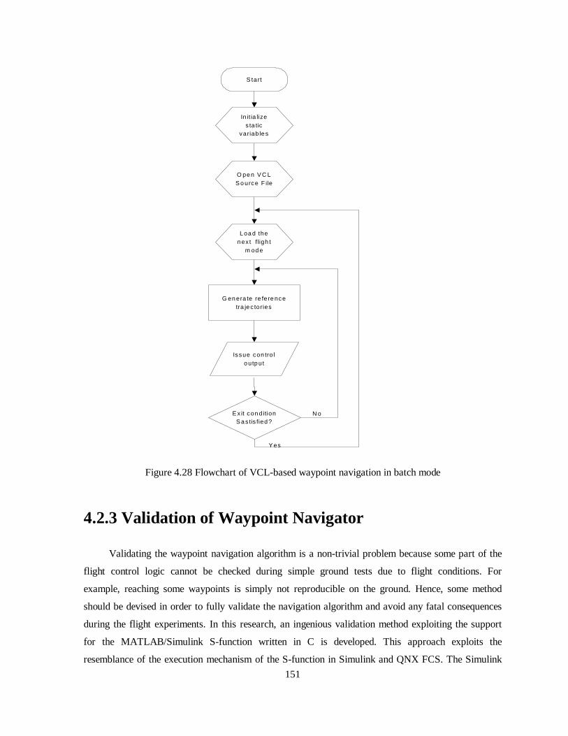
151

S tart

N o

G en era te re fere ncetra je c tories

E x it con ditionS a s tis fied ?

Y es

O pe n V C LS o urce F ile

In it ia lizes ta tic

variab le s

L oa d then ex t f ligh t

m od e

Issue con tro lo utp ut

Figure 4.28 Flowchart of VCL-based waypoint navigation in batch mode

4.2.3 Validation of Waypoint Navigator

Validating the waypoint navigation algorithm is a non-trivial problem because some part of the

flight control logic cannot be checked during simple ground tests due to flight conditions. For

example, reaching some waypoints is simply not reproducible on the ground. Hence, some method

should be devised in order to fully validate the navigation algorithm and avoid any fatal consequences

during the flight experiments. In this research, an ingenious validation method exploiting the support

for the MATLAB/Simuli nk S-function written in C is developed. This approach exploits the

resemblance of the execution mechanism of the S-function in Simulink and QNX FCS. The Simulink

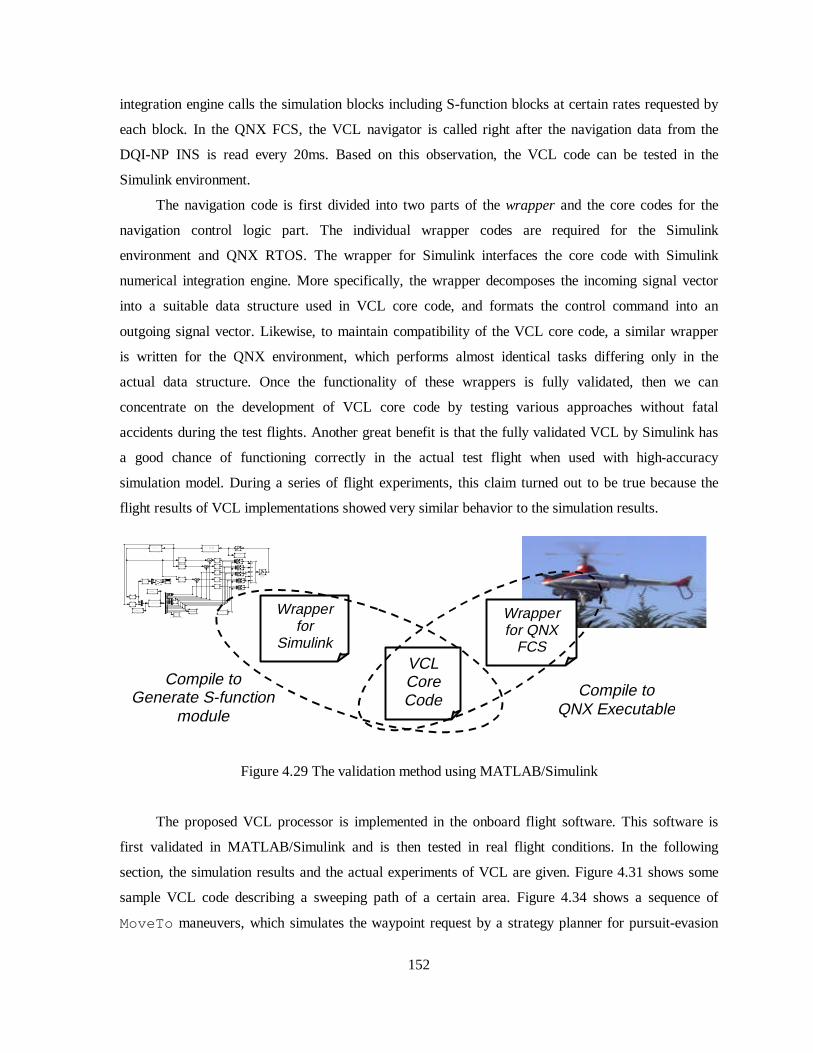
152

integration engine calls the simulation blocks including S-function blocks at certain rates requested by

each block. In the QNX FCS, the VCL navigator is called right after the navigation data from the

DQI-NP INS is read every 20ms. Based on this observation, the VCL code can be tested in the

Simulink environment.

The navigation code is first divided into two parts of the wrapper and the core codes for the

navigation control logic part. The individual wrapper codes are required for the Simulink

environment and QNX RTOS. The wrapper for Simulink interfaces the core code with Simulink

numerical integration engine. More specifically, the wrapper decomposes the incoming signal vector

into a suitable data structure used in VCL core code, and formats the control command into an

outgoing signal vector. Likewise, to maintain compatibili ty of the VCL core code, a similar wrapper

is written for the QNX environment, which performs almost identical tasks differing only in the

actual data structure. Once the functionality of these wrappers is fully validated, then we can

concentrate on the development of VCL core code by testing various approaches without fatal

accidents during the test flights. Another great benefit is that the fully validated VCL by Simulink has

a good chance of functioning correctly in the actual test flight when used with high-accuracy

simulation model. During a series of flight experiments, this claim turned out to be true because the

flight results of VCL implementations showed very similar behavior to the simulation results.

Figure 4.29 The validation method using MATLAB/Simulink

The proposed VCL processor is implemented in the onboard flight software. This software is

first validated in MATLAB/Simulink and is then tested in real flight conditions. In the following

section, the simulation results and the actual experiments of VCL are given. Figure 4.31 shows some

sample VCL code describing a sweeping path of a certain area. Figure 4.34 shows a sequence of

MoveTo maneuvers, which simulates the waypoint request by a strategy planner for pursuit-evasion

Compile toGenerate S-function

module

K

r o ll / p i t c h

Z e r o - O r d e r

H o l d

X Y G r a p h

K

V e lo c i ty

w p o u t

T o W o r k s p a c e 2

u o u t

T o W o r k s p a c e 1

s im o u t

T o W o r k s p a c e

S w i t c h 4

S w i t c h 3

S w i t c h 2

S w i t c h 1

S w i t c h

S T O P

S t o p S i m u la t io n

S e le c t o r

S e le c t o r 5

S e le c t o r

S e le c t o r 3

S e le c t o r

S e le c t o r 1

S e le c t o r

S e le c t o r

S a t u r a t io n

w a y p t n a v l2

S - F u n c t io n 1

b 2 s m e x

S - F u n c t io n

K

P o s Z

K

P o s X Y

K

M a t r ix

G a i n 1

K

M a t r ix

G a i n

x ' = A x + B u

y = C x + D u

H e l ic o p t e r M o d e l

K

H e a d in g

- 1

G a i n

0

D i s p la y

m

m

z e ro s ( 4 , 1 )

C o n s t a n t 1

VCLCore Code

Wrapperfor

Simulink

Wrapperfor QNX

FCS

Compile toQNX Executable

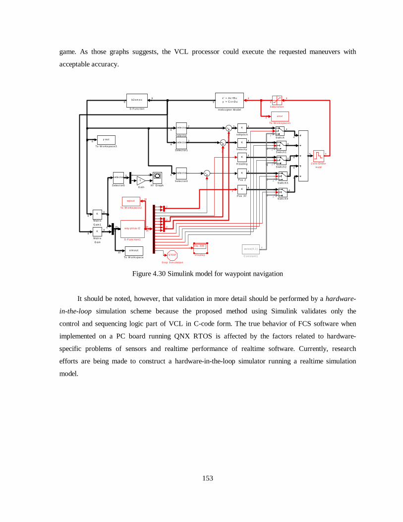
153

game. As those graphs suggests, the VCL processor could execute the requested maneuvers with

acceptable accuracy.

K

ro ll/p itc h

Z ero -O rderH old

XY G raph

K

V eloc it y

y ou t

To W orks pace3

wpout

To W orks pace2

uout

To W orks pace1

s im out

To W orks pace

S wit ch4

S wit ch3

S wit ch2

S wit ch1

S wit ch

S TO P

S top S im ula t ion

S elec t or

S elec t or5

S elec t or

S elec t or3

S elec t or

S elec t or1

S elec t or

S elec t or

S atu ra t ion

way ptnav l2

S -F unc t ion1

b2sm ex

S -F unc t ion

K

P os Z

K

P os XY

K

Matr ix

G ain1

K

Matr ix

G ain

x ' = Ax +B u y = C x+D u

H elicopte r Mode l

K

H eading

-1

G ain

053e-306

D isp lay

em ux

em ux

zeros (4 ,1 )

C ons tant 1

22

33

4

4

4

4

4

4

4 4

4

4

4

4

4

4

4

4

4

4

4

4

15

15

15

3

3

2

2

4

16

16

16

2

2

6

6

6

6

6

9

2

6

6

6

9

9

9

9

4

4

4

4

4

Figure 4.30 Simulink model for waypoint navigation

It should be noted, however, that validation in more detail should be performed by a hardware-

in-the-loop simulation scheme because the proposed method using Simulink validates only the

control and sequencing logic part of VCL in C-code form. The true behavior of FCS software when

implemented on a PC board running QNX RTOS is affected by the factors related to hardware-

specific problems of sensors and realtime performance of realtime software. Currently, research

efforts are being made to construct a hardware-in-the-loop simulator running a realtime simulation

model.

154

1 : H ov er ( 0 , 0 , 0 ) r el h eadi ng=270de g d ur at i on=10s ec ;2 : F l y To ( 0 , - 5, 0) r e l v e l =0. 5m/ s s t opov er a ut oheadi ng ;3 : H ov er ( 0 , 0 , 0 ) r el h eadi ng=0deg dur at i on=10s ec ;4 : F l y To ( 5 , 0 , 0 ) r el v el =0 . 5mps st opov er a u t ohead i ng;5 : H ov er ( 0 , 0 , 0 ) r el h eadi ng=270de g d ur at i on=10s ec ;6 : F l y To ( 0 , - 5, 0) r e l v e l =0. 5m/ s s t opov er a ut oheadi ng ;7 : H ov er ( 0 , 0 , 0 ) r el h eadi ng=180de g d ur at i on=10s ec ;8 : F l y To ( - 5, 0, 0) r e l v e l =0. 5mps s t opov er a ut oheadi ng ;9 : H ov er ( 0 , 0 , 0 ) r el h eadi ng=270de g d ur at i on=10s ec ;

10 : F l y To ( 0 , - 5, 0) r e l v e l =0. 5m/ s s t opov er a ut oheadi ng ;11 : H ov er ( 0 , 0 , 0 ) r el h eadi ng=0deg dur at i on=10s ec ;12 : F l y To ( 5 , 0 , 0 ) r el v el =0 . 5mps st opov er a u t ohead i ng;13 : H ov er ( 0 , 0 , 0 ) r el h eadi ng=270de g d ur at i on=10s ec ;

2m

4

5m

2 5m

N orth

E a st

2m

6

8

10

12

Figure 4.31 Sample VCL code for FlyTo maneuvers

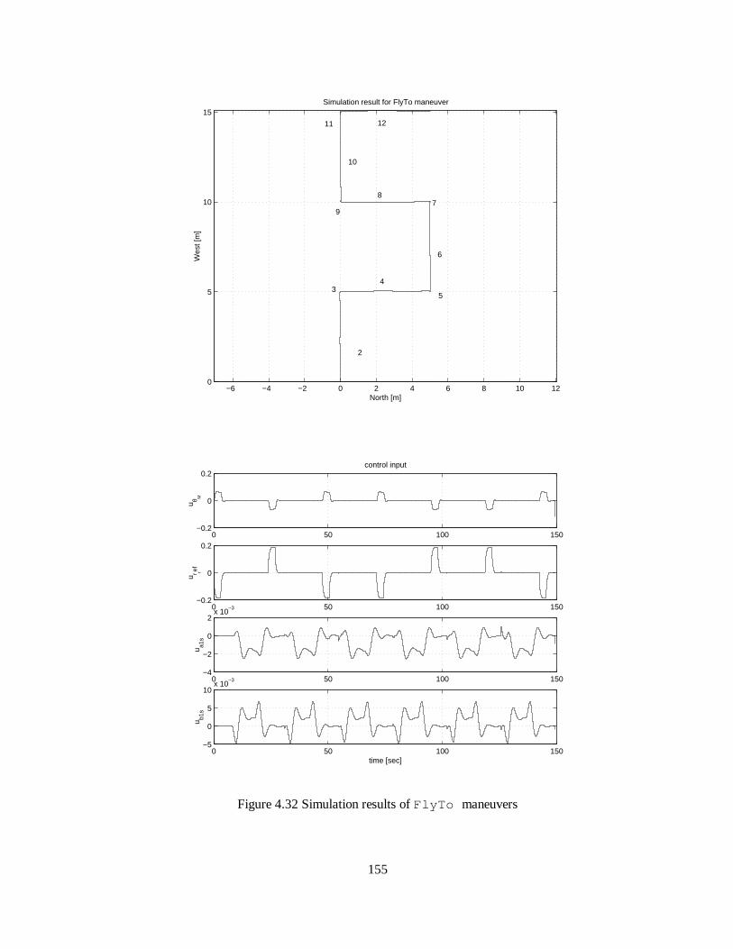
155

−6 −4 −2 0 2 4 6 8 10 120

5

10

15

North [m]

Wes

t [m

]

Simulation result for FlyTo maneuver

2

3 4

5

6

7 8

9

10

12 11

0 50 100 150−0.2

0

0.2

u θ M

control input

0 50 100 150−0.2

0

0.2

u r ref

0 50 100 150−4

−2

0

2x 10

−3

u a1s

0 50 100 150−5

0

5

10x 10

−3

u b1s

time [sec]

Figure 4.32 Simulation results of FlyTo maneuvers

156

42 44 46 48 50 52 54 56 58 6046

48

50

52

54

56

58

60

62

64X−Y map

North [m]

Wes

t [m

]

2

4

1

3 5

6

7 8

9

10

11 12

0 20 40 60 80 100 120 140 16045

50

55

Nor

th [m

]

Position−time history

0 20 40 60 80 100 120 140 16045

50

55

60

65

Wes

t [m

]

0 20 40 60 80 100 120 140 1601.2

1.3

1.4

1.5

1.6

time [sec]

Alti

tude

[m]

Figure 4.33 Experiment result of FlyTo maneuvers

157

0 20 40 60 80 100 120 140 160−5

0

5

10

Φ [d

eg]

Attitude and angular rates−time history

0 20 40 60 80 100 120 140 160−50

0

50p

[deg

/s]

0 20 40 60 80 100 120 140 160−5

0

5

Θ [d

eg]

0 20 40 60 80 100 120 140 160−20

0

20

time [sec]

q [d

eg/s

]

0 20 40 60 80 100 120 140 160−200

−100

0

Ψ [d

eg]

0 20 40 60 80 100 120 140 160−50

0

50

r [d

eg/s

]

0 20 40 60 80 100 120 140 1609000

9500

10000

10500

Eng

ine

RP

M

0 20 40 60 80 100 120 140 1600

0.02

0.04

0.06

time [sec]

GP

S S

tD [m

]

Figure 4.33 (‘cont’)

158

0 20 40 60 80 100 120 140 1601.45

1.5

1.55

1.6

u θ M

[ms]

Control input−time history

0 20 40 60 80 100 120 140 1601.2

1.4

1.6u θ T

[ms]

0 20 40 60 80 100 120 140 160−0.02

0

0.02

0.04

0.06

u a1 [m

s]

0 20 40 60 80 100 120 140 160−0.02

0

0.02

0.04

0.06

time [sec]

u b1 [m

s]

Figure 4.33 (‘cont’)

159

1 : H ov er ( 0 , 0 , 0 ) r el h eadi ng=180deg d ur at i on=7s ec ;2 : M ov eTo ( 0, - 3 , 0 ) r el v el =0. 5m/ s h eadi ng=180deg;3 : M ov eTo ( 0, 3, 0) r e l v e l= 0 . 5m/ s h ead i ng=180deg ;4 : M ov eTo ( 2, 0, 0) r e l v e l= 0 . 8m/ s h ead i ng=180deg ;5 : M ov eTo ( - 3 , 0 , 0 ) r el v el =0. 3m/ s h eadi ng=180deg;6 : M ov eTo ( 4, 4, 0) r e l v e l= 0 . 2m/ s h ead i ng=180deg ;7 : M ov eTo ( - 1 , - 2, 0) r e l ve l =0 . 2m/ s h ead i ng=180deg ;8 : M ov eTo ( - 3 , 1 , 0 ) r el v el =0. 2m/ s h eadi ng=180deg;9 : M ov eTo ( 3, - 3 , 0 ) r el v el =0. 2m/ s h eadi ng=180deg;

10 : H ov er ( 0 , 0 , 0 ) r el h eadi ng=180deg d ur at i on=7s ec ;

1m

N o rth

E a st

1m

2 3

5

87

4

6

9

Figure 4.34 Sample VCL code for MoveTo maneuvers

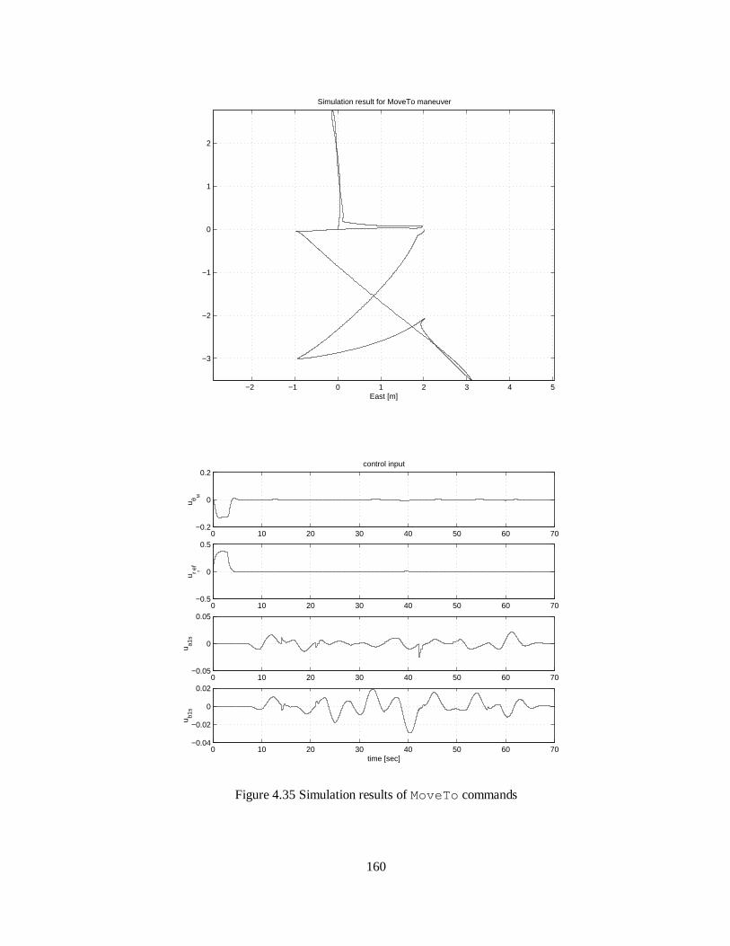
160

−2 −1 0 1 2 3 4 5

−3

−2

−1

0

1

2

East [m]

Simulation result for MoveTo maneuver

0 10 20 30 40 50 60 70−0.2

0

0.2

u θ M

control input

0 10 20 30 40 50 60 70−0.5

0

0.5

u r ref

0 10 20 30 40 50 60 70−0.05

0

0.05

u a1s

0 10 20 30 40 50 60 70−0.04

−0.02

0

0.02

time [sec]

u b1s

Figure 4.35 Simulation results of MoveTo commands

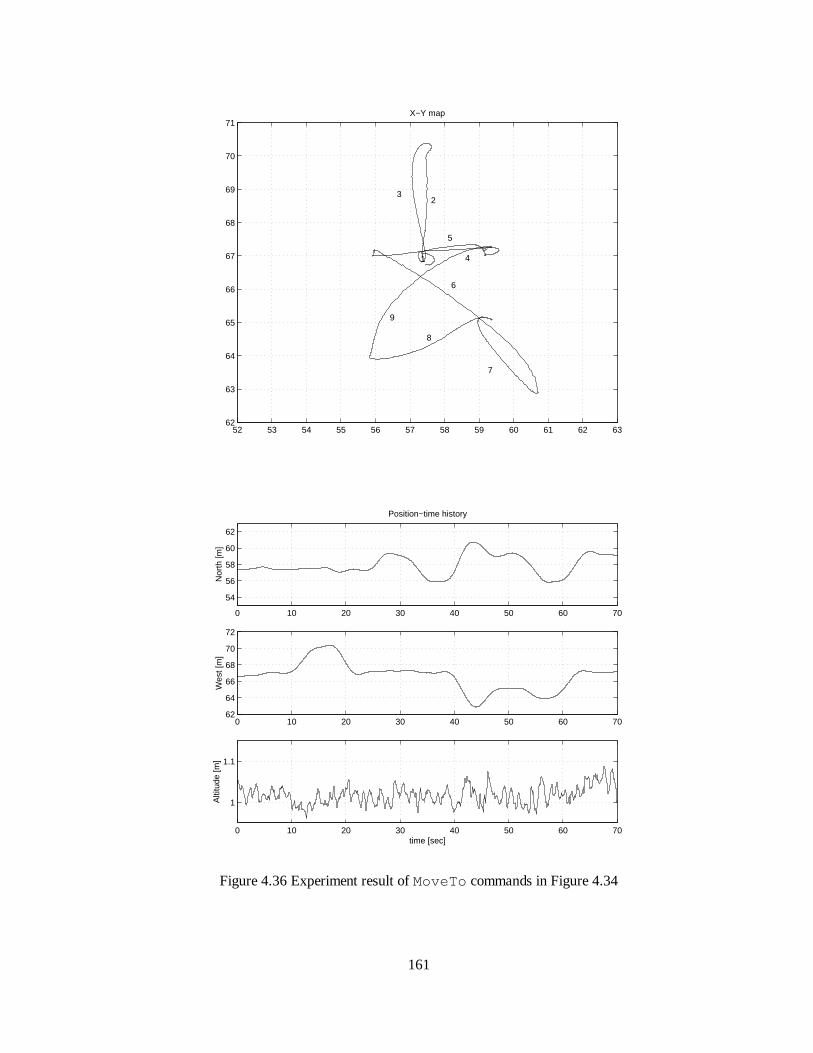
161

52 53 54 55 56 57 58 59 60 61 62 6362

63

64

65

66

67

68

69

70

71X−Y map

1

2 3

4

5

6

7

8

9

0 10 20 30 40 50 60 70

54

56

58

60

62

Nor

th [m

]

Position−time history

0 10 20 30 40 50 60 7062

64

66

68

70

72

Wes

t [m

]

0 10 20 30 40 50 60 70

1

1.1

time [sec]

Alti

tude

[m]

Figure 4.36 Experiment result of MoveTo commands in Figure 4.34

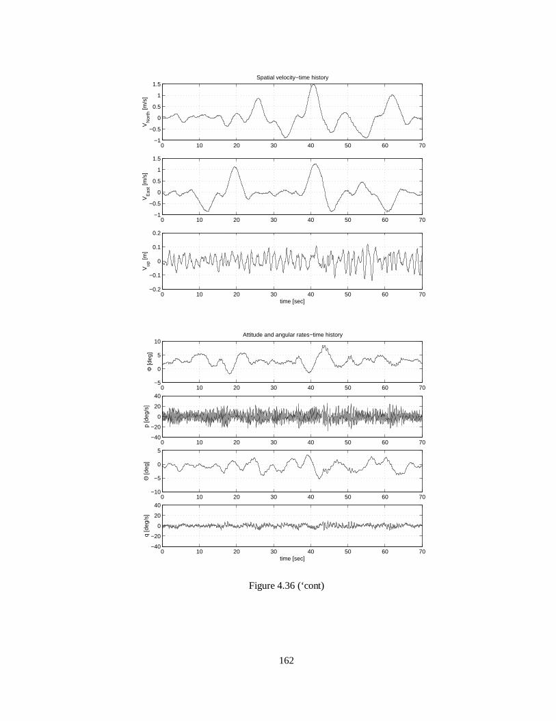
162

0 10 20 30 40 50 60 70−1

−0.5

0

0.5

1

1.5

VN

orth

[m/s

]

Spatial velocity−time history

0 10 20 30 40 50 60 70−1

−0.5

0

0.5

1

1.5

VE

ast [m

/s]

0 10 20 30 40 50 60 70−0.2

−0.1

0

0.1

0.2

time [sec]

Vup

[m]

0 10 20 30 40 50 60 70−5

0

5

10

Φ [d

eg]

Attitude and angular rates−time history

0 10 20 30 40 50 60 70−40

−20

0

20

40

p [d

eg/s

]

0 10 20 30 40 50 60 70−10

−5

0

5

Θ [d

eg]

0 10 20 30 40 50 60 70−40

−20

0

20

40

time [sec]

q [d

eg/s

]

Figure 4.36 (‘cont)

163

0 10 20 30 40 50 60 70−200

−150

−100

Ψ [d

eg]

0 10 20 30 40 50 60 70−40

−20

0

20

40r

[deg

/s]

0 10 20 30 40 50 60 709200

9400

9600

9800

Eng

ine

RP

M

0 10 20 30 40 50 60 700

0.1

0.2

time [sec]

GP

S S

tD [m

]

0 10 20 30 40 50 60 701.5

1.55

1.6

u θ M

[ms]

Control input−time history

0 10 20 30 40 50 60 701.45

1.5

1.55

1.6

u θ T

[ms]

0 10 20 30 40 50 60 70−0.02

00.020.040.060.08

u a1 [m

s]

0 10 20 30 40 50 60 70−0.02

00.020.040.060.08

time [sec]

u b1 [m

s]

Figure 4.36 (‘cont)

164

Chapter 5

5. Conclusion

This dissertation has introduced the development of a hierarchical RUAV autopilot design which has

been conducted at the University of California at Berkeley. As our goal is to build the autopilot

system hardware and software and integrate these with commercially available radio-controlled

helicopters whose dynamic model is not known a priori, the helicopter model, onboard hardware,

software, and experimental setup have been established from the bottom to the top during the last

three years. The helicopter dynamic model was found using the nonlinear aerodynamic models and

was simplified to the linear hover model. Based on this LTI model for hover, two different control

theories, classical SISO control and -synthesis control, are deployed for vehicle stabili zation. Both

of these have been tested in real flight experiment and shown reasonable performances. The controller

for hover is designed with the linear SISO multi-loop control approach. In addition to the classical

approach, the µ -synthesis attitude controller is designed and tested successfully on the Yamaha R-50.

Both of these approaches showed satisfactory results. The SISO multi-loop controller is then used as

the low-level vehicle stabili zation layer in the hierarchical structure and it is integrated with the

middle level waypoint navigator. In order to provide mission-independent universal vehicle guidance

and control interface, the novel concept of VCL is proposed and implemented in Ursa Magna 2. The

first-generation VCL system could perform, as promised, different missions whenever the associated

VCL script file is uploaded.

The research presented in this dissertation provides the footsteps for our visionary future works.

The methodology developed so far plays a crucial role in the autopilot system and the higher-level

mission scenarios will be implemented and tested on top of this work in real scale. The developed

165

methodology can be repeatedly applied to different helicopters with only minor modification and we

will be able to implement a fleet of RUAV in a networked system.

As of now, the following research topics are being investigated as the ongoing effort:

• Pursuit-evasion game

The Pursuit-evasion game is a scenario that involves a multiple number of autonomous ground-

based and aerial autonomous vehicles that are guided by central or distributed controllers. The goal of

this game is to find the evaders in a field. The pursuer should actively build a map of the terrain and a

probabili stic map to find the evaders. On the other hand, the evaders move in the field by random rule

or by active evasive motion using similar map building technology. The work proposed so far makes

it possible for the aerial vehicle to follow the waypoint commands received from the strategy planner,

whose goal is to guide the pursuers through the optimal trajectory. Currently, the VCL command for

the pursuit-evasion game is already implemented and will be integrated into the hierarchical control

system for the pursuit-evasion games.

• Vision-based navigation

As mentioned, the Ursa Magna 2 is equipped with a dedicated vision processing unit (VPU).

The VPU is now capable of color tracking and motion estimation using the color pan-tilt-zoom (PTZ)

camera and the frame grabber. The FCS is connected with the VPU via RS-232 and sends flight

information upon the request of the VPU. When the vision-based navigation is enabled, the VPU will

send the navigation command to the FCS. Currently, the color tracking and motion estimation

algorithm have been tested in real flight tests and the vision-based servoing algorithms are being

developed and tested in the simulation environment.

• Testbed for advanced wireless communication protocol

Modern autonomous agents operate solely with wireless communication links. A clumsy

umbili cal cord is a thing of the past and simply unacceptable for advanced operations. Therefore,

wireless communication is vital for the operation of unmanned autonomous vehicles. As the number

of agents increases, the management of the wireless network also becomes an important issue to

address. Currently, a joint research with Stanford Research Institute International is in progress. The

unique feature of this work is that any node can be the active agent or repeater depending on the

situation of the network. Therefore, if the some agents go out of the communication range of the base,

the communication link can still be established if there are agents between them. The in-between

166

agents automatically arm themselves as the repeaters and the communication packets can be relayed

to/from the base in a multi-hop.

Another important part is the quality of service (QoS) of the network system. Among many

aspects of the general term QoS, we are interested in the realtime nature of the wireless

communication. The QoS of the CSMA/CD protocol, which is used currently, degrades quickly if the

number of agents or the amount of data transferred increases. In some applications such as

coordinated flight, the demand for realtime communication is very high and some alternative

protocols are being sought.

• Coordinated flight

When multiple numbers of UAVs fly in a close range or in a potentially conflicting course, the

situation has to be resolved in some way. There must be some way to know the current position of the

agents in the vicinity and to estimate potential conflicts in near future. Active sensors such as vision

systems or laser range finders would be one solution to detect the nearby agents. Another way is to

exchange the information of the position of the participating agents via reliable realtime wireless

network.

• Testbed for advanced control law

As mentioned many times, the control of a helicopter is a very challenging problem. Currently,

the classical SISO approach is more widely accepted than any other advanced control theory.

However, significant improvements are expected if more advanced control theories are applied with

an accurate system model.

• Testbed for Open-Control Platform (OCP)

The current control system is implemented as proprietary system. Although there are many

research efforts on similar helicopter control problems, the actual implementations are not compatible

at all. The motivation of the OCP is the development of a unified software development and

execution platform that enables formal validation and reuse of previous work. Currently,

collaboration with the Boeing OCP team is underway and the new Ursa Maxima is planned to be the

first UAV that flies with the OCP realtime software.

As reviewed so far, the original single UAV control problem has diversified into numerous

challenging research topics. The groundwork presented in this work will enable the validation of

these research topics mentioned above through actual flight tests.

167

Appendix A Hardware Configuration of Berkeley RUAVs

A.1 Ursa Minor 3

The key design concept of Ursa Minor 3 is a low-cost, small-size and easy-to-maintain RUAV

testbed suitable for basic navigation and controller testing. The airframe itself is relatively cheaper

than other larger size RUAVs and maintenance and repair work is very easy because replacement

parts are readily available and not expensive. Limited by the small payload, the onboard hardware is

kept minimal for basic autonomous navigation solely based on INS and GPS. At first, the

communication of Ursa Minor 3 relied on the wireless modem and later it gave its way to Lucent

WaveLAN(later renamed Orinoco). The flight computer consists of single stack of PC104, consisting

of main CPU board, serial port extender, counter/timer board, custom take-over board,

Multifunction CPU Board(C yrix MediaGX 233, VGA, 2 seria l ports)

4-Serial Port Expansion Board

Counter/Timer Board (82C54)

Take-over Board

Ethernet Board

DC-DC Converter

S-VGA, Keyboard, PS-2 Mouse

ISA

BU

S (

PC

10

4)

CO M1: GPS

CO M2: W ireless Modem

CO M3: DQ I-H V

CO M4: DQ I-GPS

DC Pow er 24V

PW M In (from receiver)

PW M Out (to servos)

Optical Encoder (Engine RPM )

PW MDOU T(Relay activation)

Orinoco Ethernet converter

CO M5,6: not used

Figure A.1 Flight computer layout of Ursa Minor 3

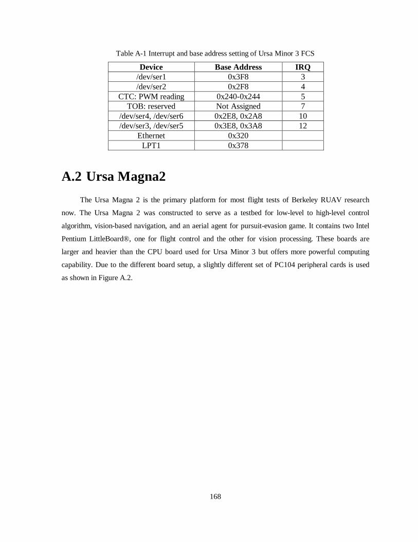
168

Table A-1 Interrupt and base address setting of Ursa Minor 3 FCS

A.2 Ursa Magna2

The Ursa Magna 2 is the primary platform for most flight tests of Berkeley RUAV research

now. The Ursa Magna 2 was constructed to serve as a testbed for low-level to high-level control

algorithm, vision-based navigation, and an aerial agent for pursuit-evasion game. It contains two Intel

Pentium LittleBoard®, one for flight control and the other for vision processing. These boards are

larger and heavier than the CPU board used for Ursa Minor 3 but offers more powerful computing

capability. Due to the different board setup, a slightly different set of PC104 peripheral cards is used

as shown in Figure A.2.

Device Base Address IRQ /dev/ser1 0x3F8 3 /dev/ser2 0x2F8 4

CTC: PWM reading 0x240-0x244 5 TOB: reserved Not Assigned 7

/dev/ser4, /dev/ser6 0x2E8, 0x2A8 10 /dev/ser3, /dev/ser5 0x3E8, 0x3A8 12

Ethernet 0x320 LPT1 0x378

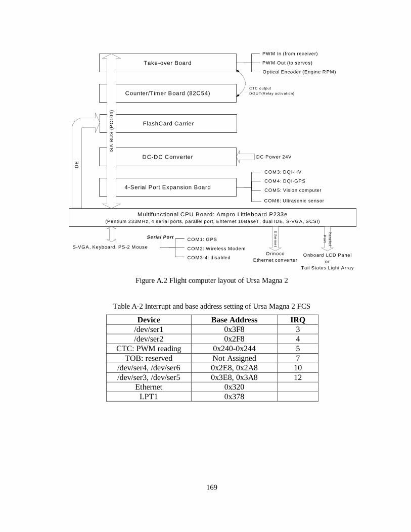
169

FlashCard Carrier

4-Serial Port Expansion Board

Counter/Timer Board (82C54)

Take-over Board

Multifunctional CPU Board: Ampro Littleboard P233e(Pentium 233MHz, 4 serial ports, parallel port, Ehternet 10BaseT, dual IDE, S-VGA, SCSI)

DC-DC Converter

S-VGA, Keyboard, PS-2 Mouse

ISA

BU

S (

PC

10

4)

COM1: GPS

COM2: Wireless Modem

COM3: DQI-HV

COM4: DQI-GPS

DC Power 24V

PW M In (from receiver)

PW M Out (to servos)

Optical Encoder (Engine R PM)

C TC outpu t

D O U T(R e lay activation)

Eth

ern

et

O rinocoEthernet converter

COM5: Vision computer

IDE

Ser ial Po r t

COM3-4: disabled

COM6: Ultrasonic sensor

Pa

ralle

l

Po

rt

Onboard LCD Panelor

Tail Status Light Array

Figure A.2 Flight computer layout of Ursa Magna 2

Table A-2 Interrupt and base address setting of Ursa Magna 2 FCS

Device Base Address IRQ /dev/ser1 0x3F8 3 /dev/ser2 0x2F8 4

CTC: PWM reading 0x240-0x244 5 TOB: reserved Not Assigned 7

/dev/ser4, /dev/ser6 0x2E8, 0x2A8 10 /dev/ser3, /dev/ser5 0x3E8, 0x3A8 12

Ethernet 0x320 LPT1 0x378

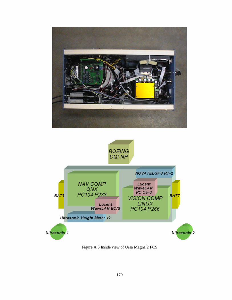
170

Figure A.3 Inside view of Ursa Magna 2 FCS

171

A.3 Ursa Maxima2

The avionics of the Ursa Maxima 2 is designed to serve as the testbed for latest research topics

such as online identification, fault tolerance, unfalsification, advanced dynamic multi-hop

communication and realtime high QoS communication system. Fully taking advantage of the ample

payload of Yamaha RMAX, the avionics contains up to four PC104 computers. In the current design,

two computers are dedicated to the flight control and background optimization. One computer is for

vision processing and another is for advanced wireless communication. These four computers

communicate one another through the onboard Ethernet hub and the communication computer serves

as the gateway of the advanced wireless communication using the Lucent Orinoco system.

Figure A.4 The information flow in the avionics of Ursa Maxima 2

172

Figure A.5 Avionics for Ursa Maxima 2

173

A.4 Servomotor Control

A servomotor is a compact electromechanical device consisting of a DC motor with a built-in

feedback circuit. These servomotors accept pulse-width modulation (PWM) signals as the reference

input. The PWM signal has fixed period and the duration of on-duty varies from 0.8 ms ~ 2.4 ms as

shown in Figure A.6.

The controlled output shaft angle is proportional to the on-duty duration of the PWM signal.

The midpoint value of 1.6 ms corresponds to the neutral position of the servo. A potentiometer that is

geared with the output shaft measures the shaft angle. This measurement is fed through a comparator

and motor driver circuit, which minimizes the difference between the actual shaft angle and the

commanded angle. In this manner, the output shaft of the servomotor is actuated to the target angle

proportional to the on-duty period while resisting the external torque.

time [msec]

Vo

lt

0.8-2.4 mson duty 14-25 ms period

Figure A.6 The characteristics of PWM signal for servomotors

The five-servo configuration is the common setup of all Berkeley RUAVs. The differences

come from the PWM characteristics of each receiver. The Kyosho and Bergen helicopters are

equipped with the receiver/servomotor system by Futaba Inc. Japan. When operated in PCM (Pulse

Coded Modulation), the period of the PWM signal is 14ms while the on-duty duration is identical to

the specification shown in Figure A.6. The PWM signals of all channels are synchronized so that the

rising edge of the PWM signals occurs at the same time. In Yamaha helicopters, however, the period

of the PWM signal is measured as 21.78 ms and the PWM signals are not synchronized as shown in

Figure A.11. The Yamaha RMAX does not require PWM signal interception because it offers a more

sophisticated interface though serial ports. The receiver status and the servo command are transmitted

by RS-232. This approach improves the reliabili ty of the overall system because the wires

transmitting the PWM signal for the servo control are not intercepted by any external custom circuits.

However, the real time performance is degraded due to the transmission time of the control data over

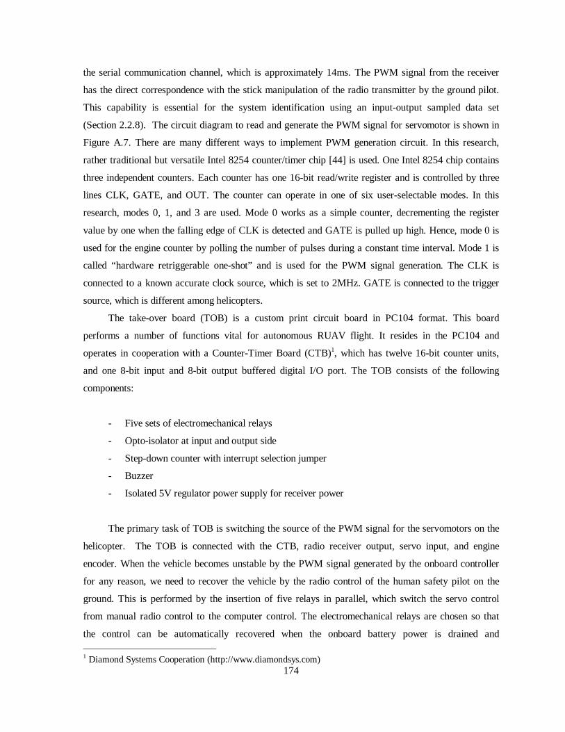
174

the serial communication channel, which is approximately 14ms. The PWM signal from the receiver

has the direct correspondence with the stick manipulation of the radio transmitter by the ground pilot.

This capabili ty is essential for the system identification using an input-output sampled data set

(Section 2.2.8). The circuit diagram to read and generate the PWM signal for servomotor is shown in

Figure A.7. There are many different ways to implement PWM generation circuit. In this research,

rather traditional but versatile Intel 8254 counter/timer chip [44] is used. One Intel 8254 chip contains

three independent counters. Each counter has one 16-bit read/write register and is controlled by three

lines CLK, GATE, and OUT. The counter can operate in one of six user-selectable modes. In this

research, modes 0, 1, and 3 are used. Mode 0 works as a simple counter, decrementing the register

value by one when the falli ng edge of CLK is detected and GATE is pulled up high. Hence, mode 0 is

used for the engine counter by polling the number of pulses during a constant time interval. Mode 1 is

called “hardware retriggerable one-shot” and is used for the PWM signal generation. The CLK is

connected to a known accurate clock source, which is set to 2MHz. GATE is connected to the trigger

source, which is different among helicopters.

The take-over board (TOB) is a custom print circuit board in PC104 format. This board

performs a number of functions vital for autonomous RUAV flight. It resides in the PC104 and

operates in cooperation with a Counter-Timer Board (CTB)1, which has twelve 16-bit counter units,

and one 8-bit input and 8-bit output buffered digital I/O port. The TOB consists of the following

components:

- Five sets of electromechanical relays

- Opto-isolator at input and output side

- Step-down counter with interrupt selection jumper

- Buzzer

- Isolated 5V regulator power supply for receiver power

The primary task of TOB is switching the source of the PWM signal for the servomotors on the

helicopter. The TOB is connected with the CTB, radio receiver output, servo input, and engine

encoder. When the vehicle becomes unstable by the PWM signal generated by the onboard controller

for any reason, we need to recover the vehicle by the radio control of the human safety pilot on the

ground. This is performed by the insertion of five relays in parallel, which switch the servo control

from manual radio control to the computer control. The electromechanical relays are chosen so that

the control can be automatically recovered when the onboard battery power is drained and

1 Diamond Systems Cooperation (http://www.diamondsys.com)

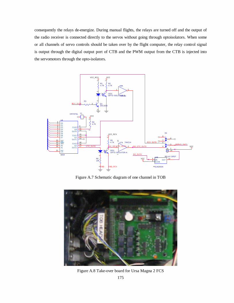
175

consequently the relays de-energize. During manual flights, the relays are turned off and the output of

the radio receiver is connected directly to the servos without going through optoisolators. When some

or all channels of servo controls should be taken over by the flight computer, the relay control signal

is output through the digital output port of CTB and the PWM output from the CTB is injected into

the servomotors through the opto-isolators.

SERVO_OUT1

VCC

R6100

12

INV_ISO_CTC_OUT0

VCC_RCV

R3

ISO_CTC_OUT0

R54.7K

12

DO_OUT0

RCV_OUT0

VCC

U7A 74HC14

1 2

147

GND

VCC_RCV

R24.7K

12

U8

8254

87654321

22231920

21

91110

151413

181617

D0D1D2D3D4D5D6D7

RDWRA0A1

CS

CLK0G0

OUT0

CLK1G1

OUT1

CLK2G2

OUT2VCC

K4

RELAY DPDT

89

7

32

4110ISO1

OPTO ISOLATOR-A

RCV_OUT0

VCC

Y1CRYSTAL

CTC_OUT0

Q12SC1815

2

3

1

GND_RCV

R14.7K

12

R44.7K

12

ISO1OPTO ISOLATOR-B

U2E

ULN2003A

59

8

12INC O MG

ND OUT

U9A

74HC14

1 2

Figure A.7 Schematic diagram of one channel in TOB

Figure A.8 Take-over board for Ursa Magna 2 FCS

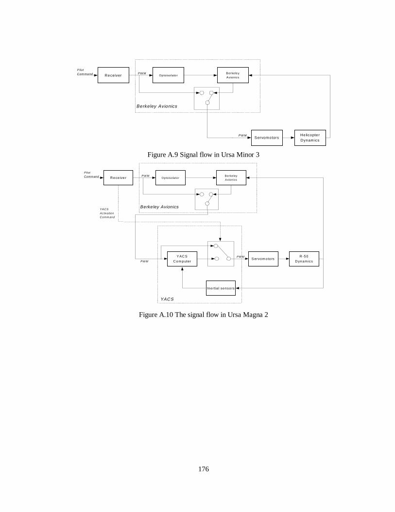
176

Optoiso lato rBerkeleyAvionics

Receiver

HelicopterDynam ics

PilotCom mand

ServomotorsPW M

Berkeley Avionics

PW M

Figure A.9 Signal flow in Ursa Minor 3

Opto iso la torBerke leyAvion ics

R ece ive r

R -50

D ynam ics

PilotComm and

PW MS ervom oto rs

Inertial sensors

Y AC S

C om puterPW M

YACSActivationComm and

YACS

Berkeley Avionics

PW M

Figure A.10 The signal flow in Ursa Magna 2

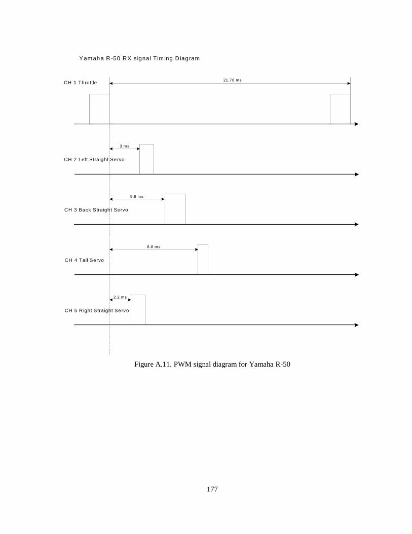
177

Yamaha R-50 RX signal Tim ing D iagram

21.78 msCH 1 Throttle

CH 2 Left Stra ight Servo

CH 3 Back Straight Servo

CH 4 Tail Servo

CH 5 Right Straight Servo

3 ms

5.6 ms

8.8 ms

2.2 ms

Figure A.11. PWM signal diagram for Yamaha R-50

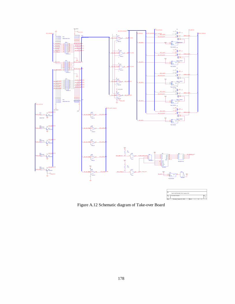
178

ISO_CTC_OUT4

U7C

74HC14

5 6

147

U2E

ULN2003A

59

8

12INCOMG

ND OUT

VCC

RCV_OUT[4:0]

INV_RCV_OUT4

RCV_OUT2

INV_RCV_OUT3

BZ1

BUZZER

JP7

HEADER 3

123

GND_RCV VCC

ISO_INV_CTC_OUT1

K4

RELAY DPDT

89

7

32

4110

C

R14RESISTOR SIP 6

123456

ISO_INV_CTC_OUT4

F_ENC_CONT_OUT

C

R13

RESISTOR SIP 6

12 3 4 5 6

VCC_RCV

CTC_OUT[4:0]

INV_RCV_OUT2

RCV_OUT[4:0]

RCV_OUT1

ISO_INV_CTC_OUT3

RCV_OUT3

K3

RELAY DPDT

89

7

32

4110

SERVO_OUT3

ISO_INV_RCV_OUT1

U5

74LS161

3456

710

291

1413121115

ABCD

ENPENTCLKLOADCLR

Q AQBQCQD

RCO

ISO_CTC_OUT4

Q42SC1815

2

3

1

VCC

VCC

RCV_OUT0ISO_CTC_OUT0

ISO_INV_RCV_OUT2

U2D

ULN2003A

49

8

13INCOMG

ND OUT

U7B

74HC14

3 4

147

R34.7K

12

D0_OUT[4:0]

ISO_INV_CTC_OUT4

CTC_GATE_SIG[4:0]

INV_RCV_OUT1

Q52SC1815

2

3

1

ISO_CTC_OUT[4:0]VCC_RCV

ISO_INV_RCV_OUT2

ISO_INV_RCV_OUT0

U2A

ULN2003A

19

8

16INCOMG

ND OUT

SERVO_OUT1

DIV_ENGINE_OUT

R15

PS2501-4

12345678 9

10111213141516

U4B

7414

3 4

ISO_INV_CTC_OUT2

U9D

74HC14

9 8

VCCR19RESISTOR

K5

RELAY DPDT

89

7

32

4110

U7D

74HC14

9 8

147

ISO_INV_RCV_OUT3

CTC_GATE_SIG1

U2B

ULN2003A

29

8

15INCOMG

ND OUT

ISO_CTC_OUT2

ISO_CTC_OUT1

CTC_OUT0

VCC

VCC_RCV

ISO_CTC_OUT1

ISO_INV_RCV_OUT0

C R11

RESISTOR SIP 6

12 3 4 5 6

CTC_OUT3

JP6

HEADER 4X2

1 23 45 67 8

ISO_INV_RCV_OUT1

SERVO_OUT[4:0]

ISO_INV_RCV_OUT4

ENC_STAB_IN

VCC_RCV

FS_SWITCH

CTC_GATE_SIG2

VCC

VCC

DO_OUT1

D0_OUT3

D0_OUT0

K2

RELAY DPDT

89

7

32

4110

U2F

ULN2003A

69

8

11INCOMG

ND OUT

4.0

TAKE OVER BOARD FOR Yamaha R-50

C

1 2Thursday, August 31, 2000

Title

Size Document Number Rev

Date: Sheet o f

VCC

ISO_CTC_OUT3

K1

RELAY DPDT

89

7

32

4110

U7A

74HC14

1 2

147

Q32SC1815

2

3

1

ISO_INV_CTC_OUT0

R25RESISTOR

R23RESISTOR

RCV_OUT4

ISO_INV_RCV_OUT3

U4A

7414

1 2

CTC_GATE_SIG0

ISO_CTC_OUT0

ISO_CTC_OUT3

C R12

RESISTOR SIP 6

12 3 4 5 6

INV_RCV_OUT0

U9A

74HC14

1 2

RCV_OUT4SERVO_OUT4

DO_OUT2

D0_OUT7

CTC_OUT1

U2C

ULN2003A

39

8

14INCOMG

ND OUT

U9C

74HC14

5 6

VCC

F_ENC_STAB_OUT

ISO_CTC_OUT[4:0]

Q22SC1815

2

3

1

CTC_GATE_SIG4

SERVO_OUT0

U9E

74HC14

11 10

147

RCV_OUT0

ISO_INV_CTC_OUT0

U7E

74HC14

11 10

147

CTC_GATE_SIG3

INV_RCV_OUT2

INV_RCV_OUT1

ISO_INV_CTC_OUT3

GND_RCV

INV_RCV_OUT0

R21RESISTOR

R16

PS2501-4

12345678 9

10111213141516

D0_OUT4

SERVO_OUT2

U9B

74HC14

3 4

RCV_OUT2

Q12SC1815

2

3

1

R27

RESISTOR

ISO_CTC_OUT2

INV_RCV_OUT4

ISO_INV_CTC_OUT1

R24.7K

12

VCC

CTC_OUT4

RCV_OUT[4:0]

RCV_OUT3

CTC_OUT2

RCV_OUT1

ISO_INV_CTC_OUT2

ISO_INV_RCV_OUT4

CTC_OUT[4:0]

R17

PS2501-4

12345678 9

10111213141516

INV_RCV_OUT3

ENC_CONT_IN

VCC

Figure A.12 Schematic diagram of Take-over Board

179

Appendix B Data Structure

A number of message formats are defined for the communication among aerial vehicles, ground

vehicles, vision processing units, and ground monitoring station. The custom messages deliver

navigation sensor reading, control output, vehicle status and so on. A message format consists of

header and body and each part has its own checksum for extended robustness and security. This type

of the data format originated from the Boeing DQI-NP and it was intended to work under streaming

data communication channel. This characteristic suits our application because our primary

communication channels are either serial communication or streamed TCP. In the following, the

general data structure and the format of individual messages are given.

• General data structure

Type Offset (byte)

Data field type Description Content

(Example)

0 WORD1 Starting marker 0X81FF (always)

2 WORD Message ID 1101(decimal)

4 WORD Data field size

6 WORD Flags

Header

8 WORD Header checksum

10 Any type Data field 1

N Any type Data field N Body

N+2 WORD Data checksum

Every message starts with the marker 0x81FF. Then the message identification number, data

field size, flags and the header checksum follow and constitute the header. The data filed size is the

number of words of the body except for the data checksum. The flag specifies various handshaking

attributes of individual message such as the acknowledge request. The checksums are computed by

the following equations:

Header checksum=-0x81FF-(Message ID)-(Data field size)-(Flags)

Data chekcsum=-(Data field 1)-….-(Data field N)

In the following, the data structures for various messages used in our research are listed

1 In this case, it is defined as 2 byte integer. (typedef short int WORD )

180

• Message 1001

Content: PWM reading of receiver and control output, engine RPM, digital input/output

Offset from Body

Data field type

Description Unit

0 WORD Receiver Chan #1 0.5 µs

2 WORD Receiver Chan #2 0.5 µs

4 WORD Receiver Chan #3 0.5 µs

6 WORD Receiver Chan #4 0.5 µs

8 WORD Receiver Chan #5 0.5 µs

10 WORD Control output Chan #1 0.5 µs

12 WORD Control output Chan #2 0.5 µs

14 WORD Control output Chan #3 0.5 µs

16 WORD Control output Chan #4 0.5 µs

18 WORD Control output Chan #5 0.5 µs

20 WORD Engine RPM Pulse count per 500ms

22 WORD Digital Input/Output

24 WORD Data checksum

• Message 1002

Content: Ultrasonic sensor readings up to four sensors.

Offset from Body

Data field type

Description Unit

0 float Ultrasonic sensor #1 m

4 float Ultrasonic sensor #2 m

8 float Ultrasonic sensor #3 m

12 float Ultrasonic sensor #4 m

16 WORD Data checksum

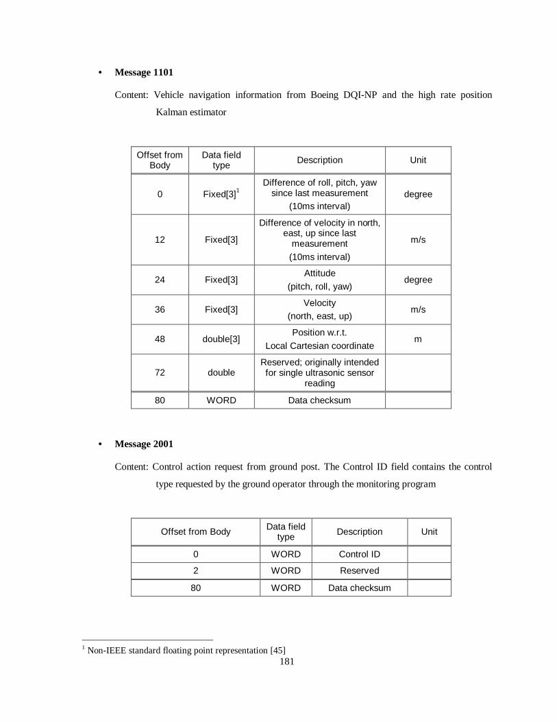
181

• Message 1101

Content: Vehicle navigation information from Boeing DQI-NP and the high rate position

Kalman estimator

Offset from Body

Data field type Description Unit

0 Fixed[3]1 Difference of roll, pitch, yaw

since last measurement (10ms interval)

degree

12 Fixed[3]

Difference of velocity in north, east, up since last

measurement

(10ms interval)

m/s

24 Fixed[3] Attitude

(pitch, roll, yaw) degree

36 Fixed[3] Velocity

(north, east, up) m/s

48 double[3] Position w.r.t.

Local Cartesian coordinate m

72 double Reserved; originally intended for single ultrasonic sensor

reading

80 WORD Data checksum

• Message 2001

Content: Control action request from ground post. The Control ID field contains the control

type requested by the ground operator through the monitoring program

Offset from Body Data field type Description Unit

0 WORD Control ID

2 WORD Reserved

80 WORD Data checksum

1 Non-IEEE standard floating point representation [45]

182

Control ID Value Description

CEM_INIT 0 The controller is just boot up and running idle

CEM_SMANUAL 1 The helicopter is being controlled manually

CEM_SMODE1 2 Controller Mode 1 is being executed

CEM_SMODE2 3 Controller Mode 2 is being executed

CEM_VCL_BATCH 11 VCL is now executed in batch mode

CEM_VCL_INTERACTIVE 12 VCL is now executed in interactive mode

CEM_ABORT -1 Abort the current control mode

• Message 4001

Content: the vehicle position, attitude, and the time stamp.

Issued by the flight computer when requested by the onboard vision computer. The

navigation information is referenced for camera coordinate computation.

Offset from Body

Data field type

Description Unit

0 double UTC sec

8 double[3] Position w.r.t.

Local Cartesian coordinate m

32 double[3] Attitude

(roll, pitch, yaw) degree

56 WORD Data checksum

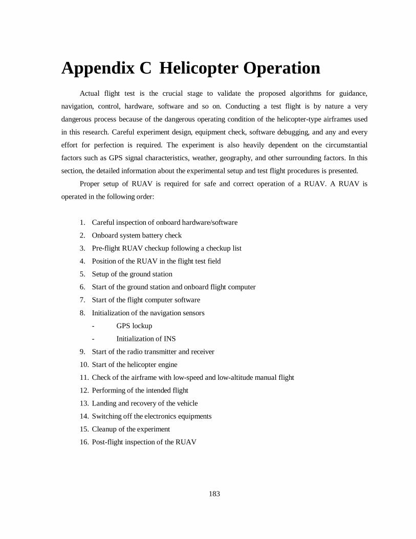
183

Appendix C Helicopter Operation

Actual flight test is the crucial stage to validate the proposed algorithms for guidance,

navigation, control, hardware, software and so on. Conducting a test flight is by nature a very

dangerous process because of the dangerous operating condition of the helicopter-type airframes used

in this research. Careful experiment design, equipment check, software debugging, and any and every

effort for perfection is required. The experiment is also heavily dependent on the circumstantial

factors such as GPS signal characteristics, weather, geography, and other surrounding factors. In this

section, the detailed information about the experimental setup and test flight procedures is presented.

Proper setup of RUAV is required for safe and correct operation of a RUAV. A RUAV is

operated in the following order:

1. Careful inspection of onboard hardware/software

2. Onboard system battery check

3. Pre-flight RUAV checkup following a checkup list

4. Position of the RUAV in the flight test field

5. Setup of the ground station

6. Start of the ground station and onboard flight computer

7. Start of the flight computer software

8. Initialization of the navigation sensors

- GPS lockup

- Initialization of INS

9. Start of the radio transmitter and receiver

10. Start of the helicopter engine

11. Check of the airframe with low-speed and low-altitude manual flight

12. Performing of the intended flight

13. Landing and recovery of the vehicle

14. Switching off the electronics equipments

15. Cleanup of the experiment

16. Post-flight inspection of the RUAV

184

Figure C.1 Aerial view of the test flight site in Richmond, California

(37.91401286,-122.33630415)

(37.91470877,-122.33620046)

(37.91502398,-122.33730990)

(37.91415614,-122.337389401)

Heli c op terTake-o ff Po s iti on

Geodes ic: (37.914397, -122.336828)LLC : (56.6584,-65.2156,-1.0039)

Helicopter Fly zone

Mis si o n Po s t

Hangar

Ori g in (Redh yd ran t)(37.91388540,-122.33609599,-26.2)

185

Figure C.2 The operation of the ground station for Berkeley UAV research

(left: notebook computer with wireless network capabili ty, monitored by Hoam Chung;

right: ground safety pilot with radio controller; the author)

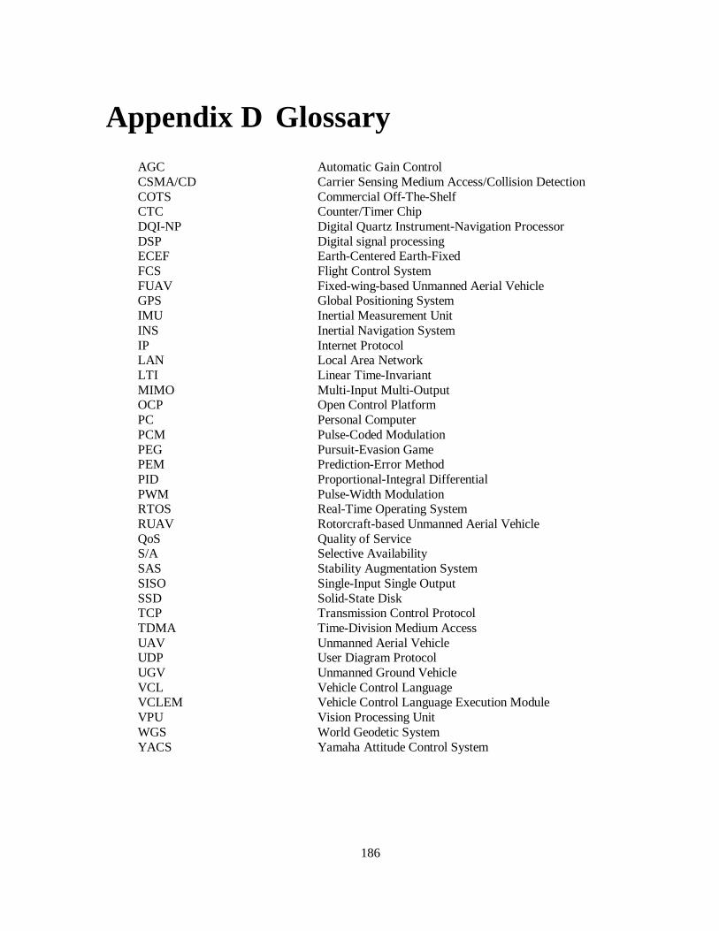
186

Appendix D Glossary

AGC Automatic Gain Control CSMA/CD Carrier Sensing Medium Access/Colli sion Detection COTS Commercial Off-The-Shelf CTC Counter/Timer Chip DQI-NP Digital Quartz Instrument-Navigation Processor DSP Digital signal processing ECEF Earth-Centered Earth-Fixed FCS Flight Control System FUAV Fixed-wing-based Unmanned Aerial Vehicle GPS Global Positioning System IMU Inertial Measurement Unit INS Inertial Navigation System IP Internet Protocol LAN Local Area Network LTI Linear Time-Invariant MIMO Multi-Input Multi-Output OCP Open Control Platform PC Personal Computer PCM Pulse-Coded Modulation PEG Pursuit-Evasion Game PEM Prediction-Error Method PID Proportional-Integral Differential PWM Pulse-Width Modulation RTOS Real-Time Operating System RUAV Rotorcraft-based Unmanned Aerial Vehicle QoS Quality of Service S/A Selective Availabili ty SAS Stabili ty Augmentation System SISO Single-Input Single Output SSD Solid-State Disk TCP Transmission Control Protocol TDMA Time-Division Medium Access UAV Unmanned Aerial Vehicle UDP User Diagram Protocol UGV Unmanned Ground Vehicle VCL Vehicle Control Language VCLEM Vehicle Control Language Execution Module VPU Vision Processing Unit WGS World Geodetic System YACS Yamaha Attitude Control System

187

Bibliography

[1] J. Lygeros, Hierarchical, Hybrid Control of Large Scale Systems, Ph. D. thesis, Department of

Electrical Engineering and Computer Sciences, University of California, Berkeley, 1996.

[2] J. Hespanha, H. J. Kim, S. Sastry, “Multiple-Agent Probabili stic Pursuit-Evasion Games,”39th

IEEE Conference on Decision and Control, pp. 3511-3516, 1999.

[3] H. Jin Kim , D. H. Shim, S. Rashid, S. Sastry, “Hierarchical System for Multiple-agent

Scenarios,” submitted to International Conference on Robotics and Automation, 2001.

[4] D. H. Shim, H. J. Kim, S. Sastry, “Hierarchical Control system Synthesis for Rotorcraft-based

Unmanned Aerial Vehicles,” AIAA Guidance, Navigation, and Control Conference, August 2000,

Denver, CO.

[5] D. H. Shim, H. J. Kim, S. Sastry, “Control System Design for Rotorcraft-based Unmanned Aerial

Vehicles using Time-domain System Identification,” Proceedings of the 2000 IEEE International

Conference on Control Applications, pp. 808-813, Anchorage, Alaska, 2000.

[6] H. Shim, T. J. Koo, F. Hoffmann, S. Sastry, “A Comprehensive Study of Control Design for an

Autonomous Helicopter,” 37th IEEE Conference on Decision and Control, pp. 3653-3658, 1998.

[7] B. Mettler, M. B. Tischler, T. Kanade, “System Identification of Small-Size Unmanned Helicopter

Dynamics,” American Helicopter Society 55th Forum, Montreal, Quebec, Canada, May 1999.

[8] D. N. Godbole, Hierarchical Hybrid Control of Automated Highway Systems, Ph. D. thesis,

Department of Electrical Engineering and Computer Sciences, University of California, Berkeley,

December, 1994.

188

[9] C. J. Tomlin, Hybrid Control of Air Traffic Management Systems, Ph.D. thesis, Department of

Electrical Engineering and Computer Sciences, University of California, Berkeley, Fall, 1998.

[10] R.W. Prouty, Helicopter Performance, Stability and Control, Krieger Publishing Company,

1995.

[11] R. K. Heffley and M. A. Mnich, Minimum-Complexity Helicopter Simulation Math Model,

NASA Contractor Report 177476, April, 1988.

[12] R. D. Murphy, K. S. Narendra, “Design of Helicopter Stabili zation Systems Using Optimal

Control Theory,” Journal of Aircraft, Vol. 6, No. 2, March-April 1969.

[13] N. K. Gupta and A. E. Bryson Jr., “Near-Hover Control of a Helicopter with a Hanging Load,”

Journal of Aircraft, Vol. 13, No. 3, March 1976.

[14] M. B. Tischler, J. D. Colbourne, M. R. Morel, D. J. Biezad, W. S. Levine and V. Moldoneanu,

“CONDUIT- A New Multidisciplinary Integration Environment for Flight Control

Development,” NASA Technical Memorandum 112203, June 1997.

[15]J. K. Peiper, S. Balilli e, and K. R. Goheen, “Linear-Quadratic Optimal Model-Following Control

of a Helicopter in Hover,” Proceedings of the American Control Conference, Baltimore, MD,

June 1994, pp. 3470-3474.

[16] W. L. Garrad, E. Low, and S. Prouty, “Design of Attitude and Rate Command Systems for

Helicopters using Eigenstructure Assignment,” Journal of Guidance, Vol. 12, No. 6, Nov.-Dec.

1989.

[17] I. Postlethwaite, A. Smerlas, D. J. Walker, A. W. Gubbels, S. W. Bailli e, M. E. Strange, and J.

Howitt, “H Control of the NRC Bell 205 Fly-by-Wire Helicopter,” Journal of the American

Helicopter Society, October 1999, pp. 276-284.

[18] D. J. Walker, and I. Postlethwaite, “Advanced Helicopter Flight Control using Two-Degree-of-

Freedom H Optimization,” Journal of Guidance, Control, and Dynamics, Vol. 19, No. 2, March-

April 1996, pp. 461-468.

189

[19] M. D. Takahashi, “H Helicopter Flight Control Law Design With and Without Rotor State

Feedback,” Journal of Guidance, Control, and Dynamics, Vol. 17, No. 6, November-December

1994, pp. 1245-1251.

[20] D. Maclay, S. J. Willi ams, “The Use of mu-Synthesis in Full Envelope Helicopter Flight Control

System Design,”

[21] W. E. Hall Jr. and A. E. Bryson Jr., “Inclusion of Rotor Dynamics in Controller Design for

Helicopters,” Journal of Aircraft, Vol. 10, No. 4, April 1973.

[22] M. D. Takahashi, “Rotor-State Feedback in the Design of Flight Control Laws for a Hovering

Helicopter,” Journal of the American Helicopter Society, Jan. 1994, pp. 50-62.

[23]S. J. Ingle, and R. Celi, “Effects of Higher Order Dynamics on Helicopter Flight Control Law

Design,” 48th Annual Forum of the American Helicopter Society, Washington, D. C., June 1992,

pp. 12- 23.

[24] K. Furuta and T. Shiotsuki, “Training Simulator of Radio Control Helicopter,” 10th IMACS

World Congress on System Simulation and Scientific Computation.

[25] J. Pallet, B. J. Wolfert, and S. Ahmad, “Real Time helicopter Flight Control Test Bed,”

Technical Report TR-EE 91-28, School of Electrical Engineering, Purdue University, 1991.

[26] H. Shim, A Study on the Design of Hovering Flight Controller for a Model Helicopter, Master’s

Thesis, Seoul National University, Seoul, Korea, 1993.

[27] J. C. Morris, M. van Nieuwstadt, and P. Bendotti, “Identification and Control of a Model

Helicopter in Hover,” Proceedings of the American Control Conference, Baltimore, MD, June

1994, pp. 1238-1242.

190

[28] H. Sira-Ramirez, M. Zribi, and S. Ahmad, “Dynamical Sliding Mode Control Approach for

Vertical Flight Regulation in Helicopters,” IEE Proceedings of Control Theory Applications, Vol.

141, January, 1994, pp. 19- 24.

[29] P. Bendotti and J. C. Morris, “Robust Control for a Model Helicopter,” Proceedings of the

American Control Conference, Seattle, Washington, June 1995, pp. 682-687.

[30] A. R. Conway, Autonomous Control of an Unstable Model Helicopter Using Carrier Phase GPS

Only, Ph. D. Thesis, Department of Electrical Engineering, Stanford University, March 1995.

[31] C. P. Sanders, P. A. DeBitetto, E. Feron, H. F. Vuong, N. Leveson, “Hierarchical Control of

Small Autonomous Helicopters,” 37th IEEE Conference on Decision and Control, pp. 3629-

3634, 1998.

[32] J. E. Corban, A. J. Calise, J. V. R. Prasad, “Implementation of Adaptive Nonlinear Control for

Flight Test on an Unmanned Helicopter,” 37th IEEE Conference on Decision and Control, pp. Pp.

3641-3646, 1998.

[33] R. T. N. Chen, M. B. Tischler, “The Role of Modeling and Flight Testing in Rotorcraft

Parameter Identification,” The 1986 AHS Forum, System Identification Session, Washington,

D.C., 1986.

[34] L. J. Ljung, Matlab System Identification Toolbox User’s Guide , The Math Works, Inc.,1997.

[35] L. J. Ljung and E. J. Ljung, System Identification: Theory for the User, 2nd ed., Prentice-Hall,

1998.

[36] J. A. Farrell and M. Barth, The Global Positioning System & Inertial Navigation, McGraw Hill ,

1998.

[37] G. M. Siouris, Aerospace Avionics Systems, Academic Press, Inc., 1993.

191

[38] J. A. Schroeder, M. B. Tischler, D. C. Watson, and M. M. Eshow, “Identification and Simulation

Evaluation of a Combat Helicopter in Hover,” Journal of Guidance, Control and Dynamics, Vol.

18, No. 1995, pp. 31-38.

[39] E. A. Fradenburgh, “The Helicopter and the Ground Effect Machine,” Journal of American

Helicopter Society, 1960, pp. 24-33.

[40] M. Sargent, and R. L. Shoemaker, The Personal Computer from the Inside Out, 3rd edition,

Addison-Wesley, 1995.

[41] R. Krten, Getting Started with QNX® 4, PARSE Software Devices, 1998.

[42] QNX Operating System- Installation & Configuration, QNX Software Systems Ltd. 1996.

[43] QNX Operating System- System Architecture, QNX Software Systems Ltd. 1996.

[44] Intel 8254 counter/timer chip user guide, Intel Press

[45] DQI-NP Integrated INS/GPS User’s Guide, Boeing Electronic Systems & Missile Defense,

1999.

[46] R. K. Mehra, S. Mahmood, and R. Waissman, “Identification of Aircraft and Rotorcraft

Aeroelastic Modes using State Space System Identification,” IEEE ????, 1995, pp. 432-437.

[47] F. L. Lewis, Optimal Estimation, John Wiley & Sons, 1986

[48] X. D. Sun, and I. Posltethwaite, “Affine LPV Modelli ng and Its Use in Gain-scheduled

Helicopter Control,” UKACC International Conference on CONTROL ’98, September, 1998, pp.

1504-1509.

[49] G. J. Balas, J. C. Doyle, K. Glover, A. Packard, R. Smith, µ-Analysis and Synthesis Toolbox

User’s Guide, The MathWorks Inc., 1995