Hierarchical Dirichlet Processes

Yee Whye Teh tehyw@comp.nus.edu.sgDepartment of Computer Science, National University of Singapore,Singapore 117543

Michael I. Jordan jordan@eecs.berkeley.eduComputer Science Division and Department of Statistics,University of California at Berkeley, Berkeley CA 94720-1776, USA

Matthew J. Beal mbeal@cse.buffalo.eduDepartment of Computer Science & Engineering,State University of New York at Buffalo, Buffalo NY 14260-2000, USA

David M. Blei blei@eecs.berkeley.eduDepartment of Computer Science, Princeton University,Princeton, NJ 08544, USA

November 15, 2005

Abstract

We consider problems involving groups of data, where each observation within a group isa draw from a mixture model, and where it is desirable to share mixture components betweengroups. We assume that the number of mixture components is unknown a priori and is to beinferred from the data. In this setting it is natural to consider sets of Dirichlet processes, onefor each group, where the well-known clustering property of the Dirichlet process provides anonparametric prior for the number of mixture components within each group. Given our desireto tie the mixture models in the various groups, we consider a hierarchical model, specificallyone in which the base measure for the child Dirichlet processes is itself distributed according toa Dirichlet process. Such a base measure being discrete, the child Dirichlet processes necessar-ily share atoms. Thus, as desired, the mixture models in the different groups necessarily sharemixture components. We discuss representations of hierarchical Dirichlet processes in terms ofa stick-breaking process, and a generalization of the Chinese restaurant process that we referto as the “Chinese restaurant franchise.” We present Markov chain Monte Carlo algorithmsfor posterior inference in hierarchical Dirichlet process mixtures, and describe applications toproblems in information retrieval and text modelling.

Keywords: clustering, mixture models, nonparametric Bayesian statistics, hierarchicalmodels, Markov chain Monte Carlo

1

1 INTRODUCTION

A recurring theme in statistics is the need to separate observations into groups, and yet allow thegroups to remain linked—to “share statistical strength.” In the Bayesian formalism such sharing isachieved naturally via hierarchical modeling; parameters are shared among groups, and the random-ness of the parameters induces dependencies among the groups. Estimates based on the posteriordistribution exhibit “shrinkage.”

In the current paper we explore a hierarchical approach to the problem of model-based clusteringof grouped data. We assume that the data are subdivided into a set of groups, and that within eachgroup we wish to find clusters that capture latent structure in the data assigned to that group. Thenumber of clusters within each group is unknown and is to be inferred. Moreover, in a sense thatwe make precise, we wish to allow clusters to be shared among the groups.

An example of the kind of problem that motivates us can be found in genetics. Consider a setof k binary markers (e.g., single nucleotide polymorphisms or “SNPs”) in a localized region of thehuman genome. While an individual human could exhibit any of 2k different patterns of markerson a single chromosome, in real populations only a small subset of such patterns—haplotypes—areactually observed (Gabriel et al. 2002). Given a meiotic model for the combination of a pair ofhaplotypes into a genotype during mating, and given a set of observed genotypes in a sample froma human population, it is of great interest to identify the underlying haplotypes (Stephens et al.2001). Now consider an extension of this problem in which the population is divided into a set ofgroups; e.g., African, Asian and European subpopulations. We may not only want to discover thesets of haplotypes within each subpopulation, but we may also wish to discover which haplotypesare shared between subpopulations. The identification of such haplotypes would have significantimplications for the understanding of the migration patterns of ancestral populations of humans.

As a second example, consider the problem from the field of information retrieval (IR) of mod-eling of relationships among sets of documents. In IR, documents are generally modeled underan exchangeability assumption, the “bag of words” assumption, in which the order of words in adocument is ignored (Salton and McGill 1983). It is also common to view the words in a documentas arising from a number of latent clusters or “topics,” where a topic is generally modeled as amultinomial probability distribution on words from some basic vocabulary (Blei et al. 2003). Thus,in a document concerned with university funding the words in the document might be drawn fromthe topics “education” and “finance.” Considering a collection of such documents, we may wishto allow topics to be shared among the documents in the corpus. For example, if the corpus alsocontains a document concerned with university football, the topics may be “education” and “sports,”and we would want the former topic to be related to that discovered in the analysis of the documenton university funding.

Moreover, we may want to extend the model to allow for multiple corpora. For example, doc-uments in scientific journals are often grouped into themes (e.g., “empirical process theory,” “mul-tivariate statistics,” “survival analysis”), and it would be of interest to discover to what extent thelatent topics that are shared among documents are also shared across these groupings. Thus ingeneral we wish to consider the sharing of clusters across multiple, nested groupings of data.

Our approach to the problem of sharing clusters among multiple, related groups is a nonpara-metric Bayesian approach, reposing on the Dirichlet process (Ferguson 1973). The Dirichlet processDP(α0, G0) is a measure on measures. It has two parameters, a scaling parameter α0 > 0 and abase probability measure G0. An explicit representation of a draw from a Dirichlet process (DP)

2

was given by Sethuraman (1994), who showed that if G ∼ DP(α0, G0), then with probability one:

G =∞∑

k=1

βkδφk, (1)

where the φk are independent random variables distributed according to G0, where δφkis an atom

at φk, and where the “stick-breaking weights” βk are also random and depend on the parameter α0

(the definition of the βk is provided in Section 3.1).The representation in (1) shows that draws from a DP are discrete (with probability one). The

discrete nature of the DP makes it unsuitable for general applications in Bayesian nonparametrics,but it is well suited for the problem of placing priors on mixture components in mixture modeling.The idea is basically to associate a mixture component with each atom in G. Introducing indica-tor variables to associate data points with mixture components, the posterior distribution yields aprobability distribution on partitions of the data. A number of authors have studied such Dirichletprocess mixture models (Antoniak 1974; Escobar and West 1995; MacEachern and Muller 1998).These models provide an alternative to methods that attempt to select a particular number of mixturecomponents, or methods that place an explicit parametric prior on the number of components.

Let us now consider the setting in which the data are subdivided into a number of groups. Givenour goal of solving a clustering problem within each group, we consider a set of random measuresGj , one for each group j, where Gj is distributed according to a group-specific Dirichlet processDP(α0j , G0j). To link these clustering problems, we link the group-specific DPs. Many authorshave considered ways to induce dependencies among multiple DPs via links among the parametersG0j and/or α0j (Cifarelli and Regazzini 1978; MacEachern 1999; Tomlinson 1998; Muller et al.2004; De Iorio et al. 2004; Kleinman and Ibrahim 1998; Mallick and Walker 1997; Ishwaran andJames 2004). Focusing on theG0j , one natural proposal is a hierarchy in which the measuresGj areconditionally independent draws from a single underlying Dirichlet process DP(α0, G0(τ)), whereG0(τ) is a parametric distribution with random parameter τ (Carota and Parmigiani 2002; Fonget al. 2002; Muliere and Petrone 1993). Integrating over τ induces dependencies among the DPs.

That this simple hierarchical approach will not solve our problem can be observed by consider-ing the case in which G0(τ) is absolutely continuous with respect to Lebesgue measure for almostall τ (e.g., G0 is Gaussian with mean τ ). In this case, given that the draws Gj arise as conditionallyindependent draws from G0(τ), they necessarily have no atoms in common (with probability one).Thus, although clusters arise within each group via the discreteness of draws from a DP, the atomsassociated with the different groups are different and there is no sharing of clusters between groups.This problem can be skirted by assuming that G0 lies in a discrete parametric family, but such anassumption would be overly restrictive.

Our proposed solution to the problem is straightforward: to force G0 to be discrete and yethave broad support, we consider a nonparametric hierarchical model in which G0 is itself a drawfrom a Dirichlet process DP(γ,H). This restores flexibility in that the modeler can choose H to becontinuous or discrete. In either case, with probability one, G0 is discrete and has a stick-breakingrepresentation as in (1). The atoms φk are shared among the multiple DPs, yielding the desiredsharing of atoms among groups. In summary, we consider the hierarchical specification:

G0 | γ,H ∼ DP(γ,H)

Gj | α0, G0 ∼ DP(α0, G0) for each j, (2)

which we refer to as a hierarchical Dirichlet process. The immediate extension to hierarchicalDirichlet process mixture models yields our proposed formalism for sharing clusters among relatedclustering problems.

3

Related nonparametric approaches to linking multiple DPs have been discussed by a number ofauthors. Our approach is a special case of a general framework for “dependent Dirichlet processes”due to MacEachern (1999) and MacEachern et al. (2001). In this framework the random variablesβk and φk in (1) are general stochastic processes (i.e., indexed collections of random variables);this allows very general forms of dependency among DPs. Our hierarchical approach fits into thisframework; we endow the stick-breaking weights βk in (1) with a second subscript indexing thegroups j, and view the weights βjk as dependent for each fixed value of k. Indeed, as we show inSection 4, the definition in (2) yields a specific, canonical form of dependence among the weightsβjk.

Our approach is also a special case of a framework referred to as analysis of densities (AnDe)by Tomlinson (1998) and Tomlinson and Escobar (2003). The AnDe model is a hierarchical modelfor multiple DPs in which the common base measure G0 is random, but rather than treating G0 asa draw from a DP, as in our case, it is treated as a draw from a mixture of DPs. The resulting G0

is continuous in general (Antoniak 1974), which, as we have discussed, is ruinous for our problemof sharing clusters. It is an appropriate choice, however, for the problem addressed by Tomlin-son (1998), which is that of sharing statistical strength among multiple sets of density estimationproblems. Thus, while the AnDe framework and our hierarchical DP framework are closely relatedformally, the inferential goal is rather different. Moreover, as we will see, our restriction to discreteG0 has important implications for the design of efficient MCMC inference algorithms.

The terminology of “hierarchical Dirichlet process” has also been used by Muller et al. (2004)to describe a different notion of hierarchy than the one discussed here. These authors consider amodel in which a coupled set of random measures Gj are defined as Gj = εF0 + (1 − ε)Fj , whereF0 and the Fj are draws from DPs. This model provides an alternative approach to sharing clusters,one in which the shared clusters are given the same stick-breaking weights (those associated withF0) in each of the groups. By contrast, in our hierarchical model, the draws Gj are based on thesame underlying base measure G0, but each draw assigns different stick-breaking weights to theshared atoms associated with G0. Thus, atoms can be partially shared.

Finally, the terminology of “hierarchical Dirichlet process” has been used in yet a third way byBeal et al. (2002) in the context of a model known as the infinite hidden Markov model, a hiddenMarkov model with a countably infinite state space. The “hierarchical Dirichlet process” of Bealet al. (2002) is, however, not a hierarchy in the Bayesian sense; rather, it is an algorithmic descriptionof a coupled set of urn models. We discuss this model in more detail in Section 7, where we showthat the notion of hierarchical DP presented here yields an elegant treatment of the infinite hiddenMarkov model.

In summary, the notion of hierarchical Dirichlet process that we explore is a specific exampleof a dependency model for multiple Dirichlet processes, one specifically aimed at the problem ofsharing clusters among related groups of data. It involves a simple Bayesian hierarchy where thebase measure for a set of Dirichlet processes is itself distributed according to a Dirichlet process.While there are many ways to couple Dirichlet processes, we view this simple, canonical Bayesianhierarchy as particularly worthy of study. Note in particular the appealing recursiveness of thedefinition; a hierarchical Dirichlet process can be readily extended to multiple hierarchical levels.This is natural in applications. For example, in our application to document modeling, one levelof hierarchy is needed to share clusters among multiple documents within a corpus, and secondlevel of hierarchy is needed to share clusters among multiple corpora. Similarly, in the geneticsexample, it is of interest to consider nested subdivisions of populations according to various criteria(geographic, cultural, economic), and to consider the flow of haplotypes on the resulting tree.

As is the case with other nonparametric Bayesian methods, a significant component of the chal-

4

lenge in working with the hierarchical Dirichlet process is computational. To provide a generalframework for designing procedures for posterior inference in the hierarchical Dirichlet processthat parallel those available for the Dirichlet process, it is necessary to develop analogs for the hi-erarchical Dirichlet process of some of the representations that have proved useful in the Dirichletprocess setting. We provide these analogs in Section 4 where we discuss a stick-breaking repre-sentation of the hierarchical Dirichlet process, an analog of the Polya urn model that we refer toas the “Chinese restaurant franchise,” and a representation of the hierarchical Dirichlet process interms of an infinite limit of finite mixture models. With these representations as background, wepresent MCMC algorithms for posterior inference under hierarchical Dirichlet process mixtures inSection 5. We present experimental results in Section 6 and present our conclusions in Section 8.

2 SETTING

We are interested in problems where the observations are organized into groups, and assumed ex-changeable both within each group and across groups. To be precise, letting j index the groups andi index the observations within each group, we assume that xj1, xj2, . . . are exchangeable withineach group j. We also assume that the observations are exchangeable at the group level, that is, ifxj = (xj1, xj2, . . .) denote all observations in group j, then x1,x2, . . . are exchangeable.

Assuming each observation is drawn independently from a mixture model, there is a mixturecomponent associated with each observation. Let θji denote a parameter specifying the mixturecomponent associated with the observation xji. We will refer to the variables θji as factors. Notethat these variables are not generally distinct; we will develop a different notation for the distinctvalues of factors. Let F (θji) denote the distribution of xji given the factor θji. Let Gj denote aprior distribution for the factors θj = (θj1, θj2, . . .) associated with group j. We assume that thefactors are conditionally independent given Gj . Thus we have the following probability model:

θji | Gj ∼ Gj for each j and i,

xji | θji ∼ F (θji) for each j and i, (3)

to augment the specification given in (2).

3 DIRICHLET PROCESSES

In this section, we provide a brief overview of Dirichlet processes. After a discussion of basicdefinitions, we present three different perspectives on the Dirichlet process: one based on the stick-breaking construction, one based on a Polya urn model, and one based on a limit of finite mixturemodels. Each of these perspectives has an analog in the hierarchical Dirichlet process, which isdescribed in Section 4.

Let (Θ,B) be a measurable space, with G0 a probability measure on the space. Let α0 be apositive real number. A Dirichlet process DP(α0, G0) is defined to be the distribution of a randomprobability measure G over (Θ,B) such that, for any finite measurable partition (A1, A2, . . . , Ar)of Θ, the random vector (G(A1), . . . , G(Ar)) is distributed as a finite-dimensional Dirichlet distri-bution with parameters (α0G0(A1), . . . , α0G0(Ar)):

(G(A1), . . . , G(Ar)) ∼ Dir(α0G0(A1), . . . , α0G0(Ar)) . (4)

We write G ∼ DP(α0, G0) if G is a random probability measure with distribution given by theDirichlet process. The existence of the Dirichlet process was established by Ferguson (1973).

5

3.1 The stick-breaking construction

Measures drawn from a Dirichlet process are discrete with probability one (Ferguson 1973). Thisproperty is made explicit in the stick-breaking construction due to Sethuraman (1994). The stick-breaking construction is based on independent sequences of i.i.d. random variables (π ′

k)∞k=1 and

(φk)∞k=1:

π′k | α0, G0 ∼ Beta(1, α0) φk | α0, G0 ∼ G0 . (5)

Now define a random measure G as

πk = π′k

k−1∏

l=1

(1 − π′l) G =∞∑

k=1

πkδφk, (6)

where δφ is a probability measure concentrated at φ. Sethuraman (1994) showed that G as definedin this way is a random probability measure distributed according to DP(α0, G0).

It is important to note that the sequence π = (πk)∞k=1 constructed by (5) and (6) satisfies

∑∞k=1 πk = 1 with probability one. Thus we may interpret π as a random probability measure on

the positive integers. For convenience, we shall write π ∼ GEM(α0) if π is a random probabilitymeasure defined by (5) and (6) (GEM stands for Griffiths, Engen and McCloskey; e.g. see Pitman2002b).

3.2 The Chinese restaurant process

A second perspective on the Dirichlet process is provided by the Polya urn scheme (Blackwell andMacQueen 1973). The Polya urn scheme shows that draws from the Dirichlet process are bothdiscrete and exhibit a clustering property.

The Polya urn scheme does not refer toG directly; it refers to draws fromG. Thus, let θ1, θ2, . . .be a sequence of i.i.d. random variables distributed according to G. That is, the variables θ1, θ2, . . .are conditionally independent given G, and hence exchangeable. Let us consider the successiveconditional distributions of θi given θ1, . . . , θi−1, where G has been integrated out. Blackwell andMacQueen (1973) showed that these conditional distributions have the following form:

θi | θ1, . . . , θi−1, α0, G0 ∼i−1∑

`=1

1

i− 1 + α0δθ`

+α0

i− 1 + α0G0 . (7)

We can interpret the conditional distributions in terms of a simple urn model in which a ball of adistinct color is associated with each atom. The balls are drawn equiprobably; when a ball is drawnit is placed back in the urn together with another ball of the same color. In addition, with probabilityproportional to α0 a new atom is created by drawing from G0 and a ball of a new color is added tothe urn.

Expression (7) shows that θi has positive probability of being equal to one of the previous draws.Moreover, there is a positive reinforcement effect; the more often a point is drawn, the more likelyit is to be drawn in the future. To make the clustering property explicit, it is helpful to introduce anew set of variables that represent distinct values of the atoms. Define φ1, . . . , φK to be the distinctvalues taken on by θ1, . . . , θi−1, and let mk be the number of values θi′ that are equal to φk for1 ≤ i′ < i. We can re-express (7) as

θi | θ1, . . . , θi−1, α0, G0 ∼K∑

k=1

mk

i− 1 + α0δφk

+α0

i− 1 + α0G0 . (8)

6

θ

G

i

xi

0G

0α

θ

Gj

γ G0

H

0α

xji

ji

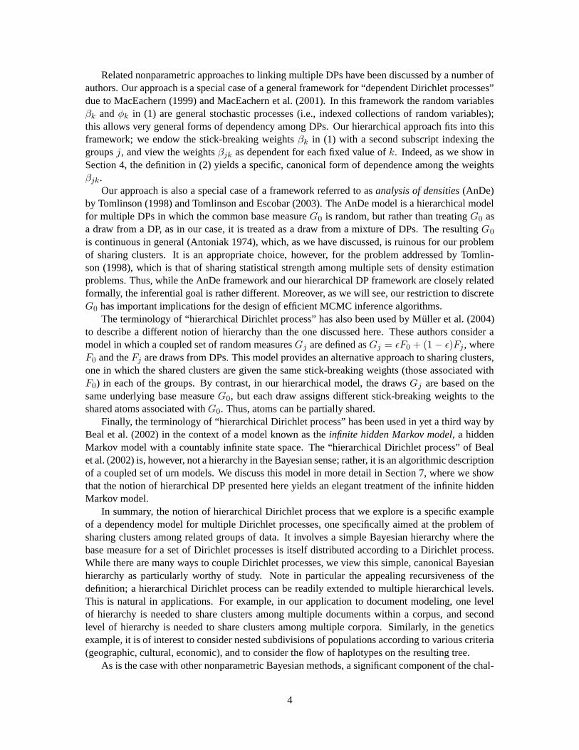
Figure 1: (Left) A representation of a Dirichlet process mixture model as a graphical model. (Right)A hierarchical Dirichlet process mixture model. In the graphical model formalism, each node in thegraph is associated with a random variable, where shading denotes an observed variable. Rectanglesdenote replication of the model within the rectangle. Sometimes the number of replicates is givenin the bottom right corner of the rectangle.

Using a somewhat different metaphor, the Polya urn scheme is closely related to a distributionon partitions known as the Chinese restaurant process (Aldous 1985). This metaphor has turnedout to be useful in considering various generalizations of the Dirichlet process (Pitman 2002a), andit will be useful in this paper. The metaphor is as follows. Consider a Chinese restaurant with anunbounded number of tables. Each θi corresponds to a customer who enters the restaurant, whilethe distinct values φk correspond to the tables at which the customers sit. The ith customer sits at thetable indexed by φk, with probability proportional to the number of customers mk already seatedthere (in which case we set θi = φk), and sits at a new table with probability proportional to α0

(increment K, draw φK ∼ G0 and set θi = φK).

3.3 Dirichlet process mixture models

One of the most important applications of the Dirichlet process is as a nonparametric prior on theparameters of a mixture model. In particular, suppose that observations xi arise as follows:

θi | G ∼ G

xi | θi ∼ F (θi) , (9)

where F (θi) denotes the distribution of the observation xi given θi. The factors θi are conditionallyindependent given G, and the observation xi is conditionally independent of the other observationsgiven the factor θi. When G is distributed according to a Dirichlet process, this model is referredto as a Dirichlet process mixture model. A graphical model representation of a Dirichlet processmixture model is shown in Figure 1 (Left).

Since G can be represented using a stick-breaking construction (6), the factors θi take on valuesφk with probability πk. We may denote this using an indicator variable zi which takes on positiveintegral values and is distributed according to π (interpreting π as a random probability measure on

7

the positive integers). Hence an equivalent representation of a Dirichlet process mixture is given bythe following conditional distributions:

π | α0 ∼ GEM(α0) zi | π ∼ π

φk | G0 ∼ G0 xi | zi, (φk)∞k=1 ∼ F (φzi

) . (10)

Moreover, G =∑∞

k=1 πkδφkand θi = φzi

.

3.4 The infinite limit of finite mixture models

A Dirichlet process mixture model can be derived as the limit of a sequence of finite mixture mod-els, where the number of mixture components is taken to infinity (Neal 1992; Rasmussen 2000;Green and Richardson 2001; Ishwaran and Zarepour 2002). This limiting process provides a thirdperspective on the Dirichlet process.

Suppose we have L mixture components. Let π = (π1, . . . πL) denote the mixing proportions.Note that we previously used the symbol π to denote the weights associated with the atoms inG. Wehave deliberately overloaded the definition of π here; as we shall see later, they are closely related.In fact, in the limit L → ∞ these vectors are equivalent up to a random size-biased permutation oftheir entries (Pitman 1996).

We place a Dirichlet prior on π with symmetric parameters (α0/L, . . . , α0/L). Let φk denotethe parameter vector associated with mixture component k, and let φk have prior distribution G0.Drawing an observation xi from the mixture model involves picking a specific mixture componentwith probability given by the mixing proportions; let zi denote that component. We thus have thefollowing model:

π | α0 ∼ Dir(α0/L, . . . , α0/L) zi | π ∼ π

φk | G0 ∼ G0 xi | zi, (φk)Lk=1 ∼ F (φzi

) . (11)

Let GL =∑L

k=1 πkδφk. Ishwaran and Zarepour (2002) show that for every measurable function f

integrable with respect to G0, we have, as L→ ∞:∫

f(θ) dGL(θ)D−→

∫

f(θ) dG(θ) . (12)

A consequence of this is that the marginal distribution induced on the observations x1, . . . , xn ap-proaches that of a Dirichlet process mixture model.

4 HIERARCHICAL DIRICHLET PROCESSES

We propose a nonparametric Bayesian approach to the modeling of grouped data, where each groupis associated with a mixture model, and where we wish to link these mixture models. By analogywith Dirichlet process mixture models, we first define the appropriate nonparametric prior, whichwe refer to as the hierarchical Dirichlet process. We then show how this prior can be used in thegrouped mixture model setting. We present analogs of the three perspectives presented earlier forthe Dirichlet process—a stick-breaking construction, a Chinese restaurant process representation,and a representation in terms of a limit of finite mixture models.

A hierarchical Dirichlet process is a distribution over a set of random probability measures over(Θ,B). The process defines a set of random probability measures Gj , one for each group, and a

8

global random probability measure G0. The global measure G0 is distributed as a Dirichlet processwith concentration parameter γ and base probability measure H:

G0 | γ,H ∼ DP(γ,H) , (13)

and the random measures Gj are conditionally independent given G0, with distributions given by aDirichlet process with base probability measure G0:

Gj | α0, G0 ∼ DP(α0, G0) . (14)

The hyperparameters of the hierarchical Dirichlet process consist of the baseline probabilitymeasure H , and the concentration parameters γ and α0. The baseline H provides the prior distribu-tion for the factors θji. The distributionG0 varies around the priorH , with the amount of variabilitygoverned by γ. The actual distribution Gj over the factors in the j th group deviates from G0, withthe amount of variability governed by α0. If we expect the variability in different groups to be dif-ferent, we can use a separate concentration parameter αj for each group j. In this paper, followingEscobar and West (1995), we put vague gamma priors on γ and α0.

A hierarchical Dirichlet process can be used as the prior distribution over the factors for groupeddata. For each j let θj1, θj2, . . . be i.i.d. random variables distributed as Gj . Each θji is a factorcorresponding to a single observation xji. The likelihood is given by:

θji | Gj ∼ Gj

xji | θji ∼ F (θji) . (15)

This completes the definition of a hierarchical Dirichlet process mixture model. The correspondinggraphical model is shown in Figure 1 (Right).

The hierarchical Dirichlet process can readily be extended to more than two levels. That is, thebase measure H can itself be a draw from a DP, and the hierarchy can be extended for as manylevels as are deemed useful. In general, we obtain a tree in which a DP is associated with each node,in which the children of a given node are conditionally independent given their parent, and in whichthe draw from the DP at a given node serves as a base measure for its children. The atoms in thestick-breaking representation at a given node are thus shared among all descendant nodes, providinga notion of shared clusters at multiple levels of resolution.

4.1 The stick-breaking construction

Given that the global measure G0 is distributed as a Dirichlet process, it can be expressed using astick-breaking representation:

G0 =∞∑

k=1

βkδφk, (16)

where φk ∼ H independently and β = (βk)∞k=1 ∼ GEM(γ) are mutually independent. Since G0

has support at the points φ = (φk)∞k=1, each Gj necessarily has support at these points as well, and

can thus be written as:

Gj =∞∑

k=1

πjkδφk. (17)

9

Let πj = (πjk)∞k=1. Note that the weights πj are independent given β (since theGj are independent

given G0). We now describe how the weights πj are related to the global weights β.Let (A1, . . . , Ar) be a measurable partition of Θ and let Kl = {k : φk ∈ Al} for l = 1, . . . , r.

Note that (K1, . . . ,Kr) is a finite partition of the positive integers. Further, assuming that H isnon-atomic, the φk’s are distinct with probability one, so any partition of the positive integers cor-responds to some partition of Θ. Thus, for each j we have:

(Gj(A1), . . . , Gj(Ar)) ∼ Dir(α0G0(A1), . . . , α0G0(Ar))

⇒

∑

k∈K1

πjk, . . . ,∑

k∈Kr

πjk

∼ Dir

α0

∑

k∈K1

βk, . . . , α0

∑

k∈Kr

βk

, (18)

for every finite partition of the positive integers. Hence each πj is independently distributed accord-ing to DP(α0,β), where we interpret β and πj as probability measures on the positive integers. IfH is non-atomic then a weaker result still holds: if πj ∼ DP(α0,β) then Gj as given in (17) is stillDP(α0, G0) distributed.

As in the Dirichlet process mixture model, since each factor θji is distributed according toGj , ittakes on the value φk with probability πjk. Again let zji be an indicator variable such that θji = φzji

.Given zji we have xji ∼ F (φzji

). Thus we obtain an equivalent representation of the hierarchicalDirichlet process mixture via the following conditional distributions:

β | γ ∼ GEM(γ)

πj | α0,β ∼ DP(α0,β) zji | πj ∼ πj

φk | H ∼ H xji | zji, (φk)∞k=1 ∼ F (φzji

) . (19)

We now derive an explicit relationship between the elements of β and πj . Recall that the stick-breaking construction for Dirichlet processes defines the variables βk in (16) as follows:

β′k ∼ Beta(1, γ) βk = β′k

k−1∏

l=1

(1 − β′l) . (20)

Using (18), we show that the following stick-breaking construction produces a random probabilitymeasure πj ∼ DP(α0,β):

π′jk ∼ Beta

(

α0βk, α0

(

1 −k∑

l=1

βl

))

πjk = π′jk

k−1∏

l=1

(1 − π′jl) . (21)

To derive (21), first notice that for a partition ({1, . . . , k − 1}, {k}, {k + 1, k + 2, . . .}), (18) gives:(

k−1∑

l=1

πjl, πjk,∞∑

l=k+1

πjl

)

∼ Dir

(

α0

k−1∑

l=1

βl, α0βk, α0

∞∑

l=k+1

βl

)

. (22)

Removing the first element, and using standard properties of the Dirichlet distribution, we have:

1

1 −∑k−1

l=1 πjl

(

πjk,

∞∑

l=k+1

πjl

)

∼ Dir

(

α0βk, α0

∞∑

l=k+1

βl

)

. (23)

Finally, define π′jk =πjk

1−∑k−1

l=1πjl

and observe that 1 −∑k

l=1 βl =∑∞

l=k+1 βl to obtain (21).

Together with (20), (16) and (17), this completes the description of the stick-breaking constructionfor hierarchical Dirichlet processes.

10

φ

φφ

22

21 23

24

26

25 27

28

33

34

31

32

3536

= =ψ12 =ψ

=ψ=ψ =ψ =ψ

=ψ=ψ

11 131 2 1

3 121 22 23 24

31

3 1

1 232

ψ

θθ

θ θ

θθ

θθ

θ

θ θθ

17

15

16

1211

13

1418

θθθ

θθθθθ

φ φ

φφ φ φ

φφ

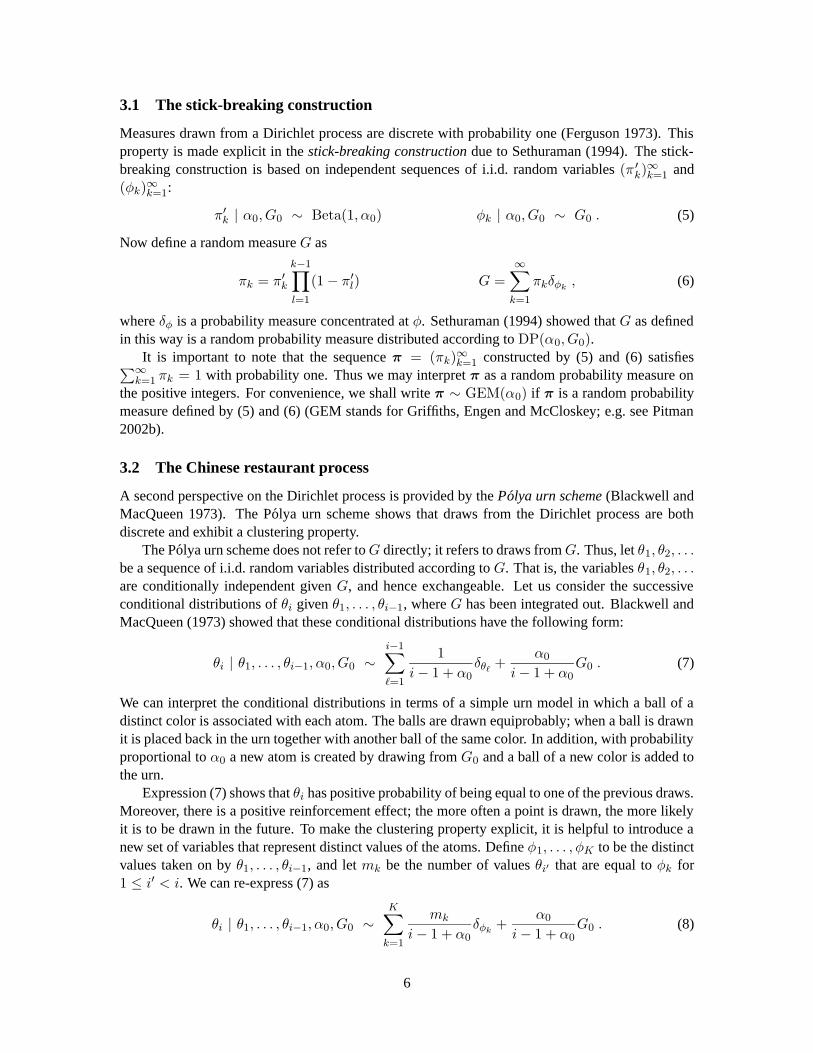
Figure 2: A depiction of a Chinese restaurant franchise. Each restaurant is represented by a rectan-gle. Customers (θji’s) are seated at tables (circles) in the restaurants. At each table a dish is served.The dish is served from a global menu (φk), whereas the parameter ψjt is a table-specific indicatorthat serves to index items on the global menu. The customer θji sits at the table to which it has beenassigned in (24).

4.2 The Chinese restaurant franchise

In this section we describe an analog of the Chinese restaurant process for hierarchical Dirichletprocesses that we refer to as the Chinese restaurant franchise. In the Chinese restaurant franchise,the metaphor of the Chinese restaurant process is extended to allow multiple restaurants which sharea set of dishes.

The metaphor is as follows (see Figure 2). We have a restaurant franchise with a shared menuacross the restaurants. At each table of each restaurant one dish is ordered from the menu by thefirst customer who sits there, and it is shared among all customers who sit at that table. Multipletables in multiple restaurants can serve the same dish.

In this setup, the restaurants correspond to groups and the customers correspond to the factorsθji. We also let φ1, . . . , φK denote K i.i.d. random variables distributed according to H; this is theglobal menu of dishes. We also introduce variables ψjt which represent the table-specific choice ofdishes; in particular, ψjt is the dish served at table t in restaurant j.

Note that each θji is associated with one ψjt, while each ψjt is associated with one φk. Weintroduce indicators to denote these associations. In particular, let tji be the index of the ψjt associ-ated with θji, and let kjt be the index of φk associated with ψjt. In the Chinese restaurant franchisemetaphor, customer i in restaurant j sat at table tji while table t in restaurant j serves dish kjt.

We also need a notation for counts. In particular, we need to maintain counts of customers andcounts of tables. We use the notation njtk to denote the number of customers in restaurant j attable t eating dish k. Marginal counts are represented with dots. Thus, njt· represents the numberof customers in restaurant j at table t and nj·k represents the number of customers in restaurant jeating dish k. The notation mjk denotes the number of tables in restaurant j serving dish k. Thus,mj· represents the number of tables in restaurant j,m·k represents the number of tables serving dishk, and m·· the total number of tables occupied.

Let us now compute marginals under a hierarchical Dirichlet process when G0 and Gj are

11

integrated out. First consider the conditional distribution for θji given θj1, . . . , θj,i−1 andG0, whereGj is integrated out. From (8):

θji | θj1, . . . , θj,i−1, α0, G0 ∼

mj·∑

t=1

njt·i− 1 + α0

δψjt+

α0

i− 1 + α0G0 , (24)

This is a mixture, and a draw from this mixture can be obtained by drawing from the terms on theright-hand side with probabilities given by the corresponding mixing proportions. If a term in thefirst summation is chosen then we set θji = ψjt and let tji = t for the chosen t. If the second termis chosen then we increment mj· by one, draw ψjmj·

∼ G0 and set θji = ψjmj·and tji = mj·.

Now we proceed to integrate out G0. Notice that G0 appears only in its role as the distributionof the variables ψjt. Since G0 is distributed according to a Dirichlet process, we can integrate it outby using (8) again and write the conditional distribution of ψjt as:

ψjt | ψ11, ψ12, . . . , ψ21, . . . , ψj t−1, γ,H ∼K∑

k=1

m·k

m·· + γδφk

+γ

m·· + γH . (25)

If we draw ψjt via choosing a term in the summation on the right-hand side of this equation, we setψjt = φk and let kjt = k for the chosen k. If the second term is chosen then we increment K byone, draw φK ∼ H and set ψjt = φK and kjt = K.

This completes the description of the conditional distributions of the θji variables. To use theseequations to obtain samples of θji, we proceed as follows. For each j and i, first sample θji using(24). If a new sample from G0 is needed, we use (25) to obtain a new sample ψjt and set θji = ψjt.

Note that in the hierarchical Dirichlet process the values of the factors are shared between thegroups, as well as within the groups. This is a key property of hierarchical Dirichlet processes.

4.3 The infinite limit of finite mixture models

As in the case of a Dirichlet process mixture model, the hierarchical Dirichlet process mixture modelcan be derived as the infinite limit of finite mixtures. In this section, we present two apparentlydifferent finite models that both yield the hierarchical Dirichlet process mixture in the infinite limit,each emphasizing a different aspect of the model.

Consider the following collection of finite mixture models, where β is a global vector of mixingproportions and πj is a group-specific vector of mixing proportions:

β | γ ∼ Dir(γ/L, . . . , γ/L)

πj | α0,β ∼ Dir(α0β) zji | πj ∼ πj

φk | H ∼ H xji | zji, (φk)Lk=1 ∼ F (φzji

) . (26)

The parametric hierarchical prior for β and π in (26) has been discussed by MacKay and Peto(1994) as a model for natural languages. We will show that the limit of this model as L→ ∞ is thehierarchical Dirichlet process. Let us consider the random probability measuresGL

0 =∑L

k=1 βkδφk

andGLj =∑L

k=1 πjkδφk. As in Section 3.4, for every measurable function f integrable with respect

to H we have∫

f(θ) dGL0 (θ)D−→

∫

f(θ) dG0(θ) , (27)

12

as L → ∞. Further, using standard properties of the Dirichlet distribution, we see that (18) stillholds for the finite case for partitions of {1, . . . , L}; hence we have:

GLj ∼ DP(α0, GL0 ) . (28)

It is now clear that as L → ∞ the marginal distribution this finite model induces on x approachesthe hierarchical Dirichlet process mixture model.

There is an alternative finite model whose limit is also the hierarchical Dirichlet process mixturemodel. Instead of introducing dependencies between the groups by placing a prior on β (as in thefirst finite model), each group can instead choose a subset of T mixture components from a model-wide set of L mixture components. In particular consider the following model:

β | γ ∼ Dir(γ/L, . . . , γ/L) kjt | β ∼ β

πj | α0 ∼ Dir(α0/T, . . . , α0/T ) tji | πj ∼ πj

φk | H ∼ H xji | tji, (kjt)Tt=1, (φk)

Lk=1 ∼ F (φkjtji

) . (29)

As T → ∞ and L → ∞, the limit of this model is the Chinese restaurant franchise process; hencethe infinite limit of this model is also the hierarchical Dirichlet process mixture model.

5 INFERENCE

In this section we describe three related Markov chain Monte Carlo sampling schemes for the hi-erarchical Dirichlet process mixture model. The first is a straightforward Gibbs sampler based onthe Chinese restaurant franchise, the second is based upon an augmented representation involvingboth the Chinese restaurant franchise and the posterior for G0, while the third is a variation on thesecond sampling scheme with streamlined bookkeeping. To simplify the discussion we assume thatthe base distribution H is conjugate to the data distribution F ; this allows us to focus on the issuesspecific to the hierarchical Dirichlet process. The nonconjugate case can be approached by adapt-ing to the hierarchical Dirichlet process techniques developed for nonconjugate DP mixtures (Neal2000). Moreover, in this section we assume fixed values for the concentration parameters α0 and γ;we present a sampler for these parameters in the appendix.

We recall the random variables of interest. The variables xji are the observed data. Each xjiis assumed to arise as a draw from a distribution F (θji). Let the factor θji be associated withthe table tji in the restaurant representation; i.e., let θji = ψjtji

. The random variable ψjt is aninstance of mixture component kjt; i.e., ψjt = φkjt

. The prior over the parameters φk is H . Letzji = kjtji

denote the mixture component associated with the observation xji. We use the notationnjtk to denote the number of customers in restaurant j at table t eating dish k, while mjk denotesthe number of tables in restaurant j serving dish k. Marginal counts are represented with dots.

Let x = (xji : all j, i), xjt = (xji : all i with tji = t), t = (tji : all j, i), k = (kjt : all j, t),z = (zji : all j, i), m = (mjk : all j, k) and φ = (φ1, . . . , φK). When a superscript is attachedto a set of variables or a count, e.g., x−ji, k−jt or n−jijt· , this means that the variable correspondingto the superscripted index is removed from the set or from the calculation of the count. In theexamples, x−ji = x\xji, k−jt = k\kjt and n−jijt· is the number of observations in group j whosefactor is associated with ψjt, leaving out item xji.

Let F (θ) have density f(·|θ) and H have density h(·). Since H is conjugate to F we integrateout the mixture component parameters φ in the sampling schemes. Denote the conditional density

13

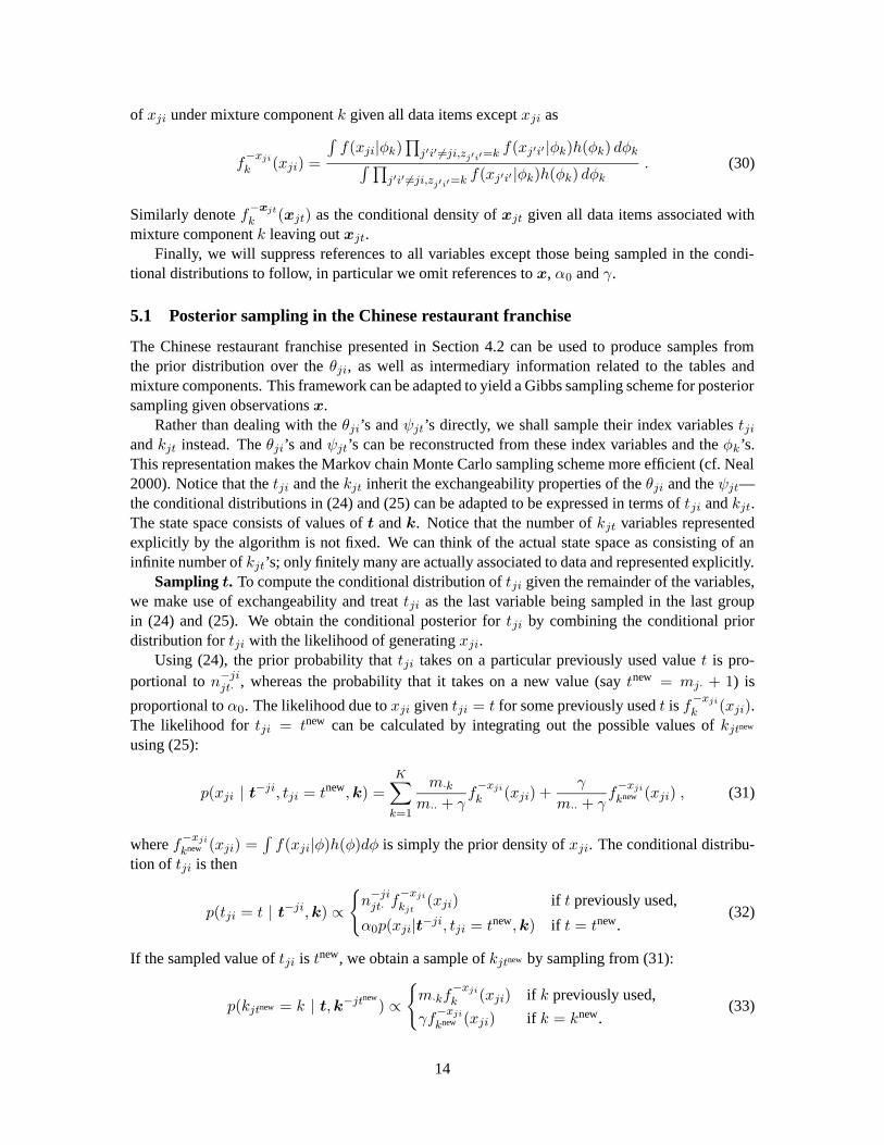
of xji under mixture component k given all data items except xji as

f−xji

k (xji) =

∫

f(xji|φk)∏

j′i′ 6=ji,zj′i′=kf(xj′i′ |φk)h(φk) dφk

∫∏

j′i′ 6=ji,zj′i′=kf(xj′i′ |φk)h(φk) dφk

. (30)

Similarly denote f−xjt

k (xjt) as the conditional density of xjt given all data items associated withmixture component k leaving out xjt.

Finally, we will suppress references to all variables except those being sampled in the condi-tional distributions to follow, in particular we omit references to x, α0 and γ.

5.1 Posterior sampling in the Chinese restaurant franchise

The Chinese restaurant franchise presented in Section 4.2 can be used to produce samples fromthe prior distribution over the θji, as well as intermediary information related to the tables andmixture components. This framework can be adapted to yield a Gibbs sampling scheme for posteriorsampling given observations x.

Rather than dealing with the θji’s and ψjt’s directly, we shall sample their index variables tjiand kjt instead. The θji’s and ψjt’s can be reconstructed from these index variables and the φk’s.This representation makes the Markov chain Monte Carlo sampling scheme more efficient (cf. Neal2000). Notice that the tji and the kjt inherit the exchangeability properties of the θji and the ψjt—the conditional distributions in (24) and (25) can be adapted to be expressed in terms of tji and kjt.The state space consists of values of t and k. Notice that the number of kjt variables representedexplicitly by the algorithm is not fixed. We can think of the actual state space as consisting of aninfinite number of kjt’s; only finitely many are actually associated to data and represented explicitly.

Sampling t. To compute the conditional distribution of tji given the remainder of the variables,we make use of exchangeability and treat tji as the last variable being sampled in the last groupin (24) and (25). We obtain the conditional posterior for tji by combining the conditional priordistribution for tji with the likelihood of generating xji.

Using (24), the prior probability that tji takes on a particular previously used value t is pro-portional to n−jijt· , whereas the probability that it takes on a new value (say tnew = mj· + 1) is

proportional to α0. The likelihood due to xji given tji = t for some previously used t is f−xji

k (xji).The likelihood for tji = tnew can be calculated by integrating out the possible values of kjtnew

using (25):

p(xji | t−ji, tji = tnew,k) =K∑

k=1

m·k

m·· + γf−xji

k (xji) +γ

m·· + γf−xji

knew (xji) , (31)

where f−xji

knew (xji) =∫

f(xji|φ)h(φ)dφ is simply the prior density of xji. The conditional distribu-tion of tji is then

p(tji = t | t−ji,k) ∝

{

n−jijt· f−xji

kjt(xji) if t previously used,

α0p(xji|t−ji, tji = tnew,k) if t = tnew.

(32)

If the sampled value of tji is tnew, we obtain a sample of kjtnew by sampling from (31):

p(kjtnew = k | t,k−jtnew) ∝

{

m·kf−xji

k (xji) if k previously used,

γf−xji

knew (xji) if k = knew.(33)

14

If as a result of updating tji some table t becomes unoccupied, i.e., njt· = 0, then the probabilitythat this table will be reoccupied in the future will be zero, since this is always proportional to njt·.As a result, we may delete the corresponding kjt from the data structure. If as a result of deletingkjt some mixture component k becomes unallocated, we delete this mixture component as well.

Sampling k. Since changing kjt actually changes the component membership of all data itemsin table t, the likelihood obtained by setting kjt = k is given by f

−xjt

k (xjt), so that the conditionalprobability of kjt is

p(kjt = k | t,k−jt) ∝

{

m−jt·k f

−xjt

k (xjt) if k is previously used,

γf−xjt

knew (xjt) if k = knew.(34)

5.2 Posterior sampling with an augmented representation

In the Chinese restaurant franchise sampling scheme, the sampling for all groups is coupled sinceG0 is integrated out. This complicates matters in more elaborate models (e.g., in the case of thehidden Markov model considered in Section 7). In this section we describe an alternative samplingscheme where in addition to the Chinese restaurant franchise representation, G0 is instantiated andsampled from so that the posterior conditioned on G0 factorizes across groups.

Given a posterior sample (t, k) from the Chinese restaurant franchise representation, we canobtain a draw from the posterior of G0 by noting that G0 ∼ DP(γ,H) and ψjt for each table t is a

draw from G0. Conditioning on the ψjt’s, G0 is now distributed as DP(γ +m··,γH+

∑Kk=1

m·kδφk

γ+m··

).An explicit construction for G0 is now given as

β = (β1, . . . , βK , βu) ∼ Dir(m·1, . . . ,m·K , γ) Gu ∼ DP(γ,H)

p(φk | t,k) ∝ h(φk)∏

ji:kjtji=k

f(xji|φk) G0 =K∑

k=1

βkδφk+ βuGu (35)

Given a sample of G0 the posterior for each group is factorized and sampling in each group canbe performed separately. The variables of interest in this scheme are t and k as in the Chineserestaurant franchise sampling scheme and β above, while both φ and Gu are integrated out (thisintroduces couplings into the sampling for each group but is easily handled).

Sampling for t and k is almost identical to the Chinese restaurant franchise sampling scheme.The only novelty is that we replace m·k by βk and γ by βu in (31), (32), (33) and (34), and whena new component knew is instantiated we draw b ∼ Beta(1, γ) and set βknew = bβu and βnew

u =(1− b)βu. We can understand b as follows: when a new component is instantiated, it is instantiatedfrom Gu by choosing an atom in Gu with probability given by its weight b. Using the fact that thesequence of stick-breaking weights is a size-biased permutation of the weights in a draw from aDirichlet process (Pitman 1996), the weight b corresponding to the chosen atom in Gu will have thesame distribution as the first stick-breaking weight, i.e., Beta(1, γ).

Sampling for β has already been described in (35):

(β1, . . . , βK , βu) | t,k ∼ Dir(m·1, . . . ,m·K , γ) . (36)

5.3 Posterior sampling by direct assignment

In both the Chinese restaurant franchise and augmented representation sampling schemes, data itemsare first assigned to some table tji, and the tables are then assigned to some mixture component kjt.

15

This indirect association to mixture components can make the bookkeeping somewhat involved. Inthis section we describe a variation on the augmented representation sampling scheme that directlyassigns data items to mixture components via a variable zji which is equivalent to kjtji

in the earliersampling schemes. The tables are only represented in terms of the numbers of tables mjk.

Sampling z can be realized by grouping together terms associated with each k in (31) and (32):

p(zji = k | z−ji,m,β) =

{

(n−jij·k + α0βk)f−xji

k (xji) if k previously used,

α0βuf−xji

knew (xji) if k = knew.(37)

where we have replaced m·k with βk and γ with βu.Sampling m. In the augmented representation sampling scheme, conditioned on the assignment

of data items to mixture components z, the only effect of t and k on other variables is via m inthe conditional distribution of β in (36). As a result it is sufficient to sample m in place of t andk. To obtain the distribution of mjk conditioned on other variables, consider the distribution of tjiassuming that kjtji

= zji. The probability that data item xji is assigned to some table t such thatkjt = k is

p(tji = t|kjt = k, t−ji,k,β) ∝ n−jijt· , (38)

while the probability that it is assigned a new table under component k is

p(tji = tnew|kjtnew = k, t−ji,k,β) ∝ α0βk . (39)

These equations form the conditional distributions of a Gibbs sampler whose equilibrium distribu-tion is the prior distribution over the assignment of nj·k observations to components in an ordinaryDirichlet process with concentration parameter α0βk. The corresponding distribution over the num-ber of components is then the desired conditional distribution of mjk. Antoniak (1974) has shownthat this is:

p(mjk = m | z,m−jk,β) =Γ(α0βk)

Γ(α0βk + nj·k)s(nj·k,m)(α0βk)

m , (40)

where s(n,m) are unsigned Stirling numbers of the first kind. We have by definition that s(0, 0) =s(1, 1) = 1, s(n, 0) = 0 for n > 0 and s(n,m) = 0 for m > n. Other entries can be computed ass(n+ 1,m) = s(n,m− 1) + ns(n,m).

Sampling for β is the same as in the augmented sampling scheme and is given by (36).

5.4 Comparison of Sampling Schemes

Let us now consider the relative merits of these three sampling schemes. In terms of ease of im-plementation, the direct assignment scheme is preferred because its bookkeeping is straightforward.The two schemes based on the Chinese restaurant franchise involve more substantial effort. In ad-dition, both the augmented and direct assignment schemes sample rather than integrate out G0, andas a result the sampling of the groups is decoupled given G0. This simplifies the sampling schemesand makes them applicable in elaborate models such as the hidden Markov model in Section 7.

In terms of convergence speed, the direct assignment scheme changes the component mem-bership of data items one at a time, while in both schemes using the Chinese restaurant franchisechanging the component membership of one table will change the membership of multiple dataitems at the same time, leading to potentially improved performance. This is akin to split-and-merge

16

techniques in Dirichlet process mixture modeling (Jain and Neal 2000). This analogy is, however,somewhat misleading in that unlike split-and-merge methods, the assignment of data items to tablesis a consequence of the prior clustering effect of a Dirichlet process with nj·k samples. As a result,we expect that the probability of obtaining a successful reassignment of a table to another previ-ously used component will often be small, and we do not necessarily expect the Chinese restaurantfranchise schemes to dominate the direct assignment scheme.

The inference methods presented here should be viewed as first steps in the development ofinference procedures for hierarchical Dirichlet process mixtures. More sophisticated methods—such as split-and-merge methods (Jain and Neal 2000) and variational methods (Blei and Jordan2005)—have shown promise for Dirichlet processes and we expect that they will prove useful forhierarchical Dirichlet processes as well.

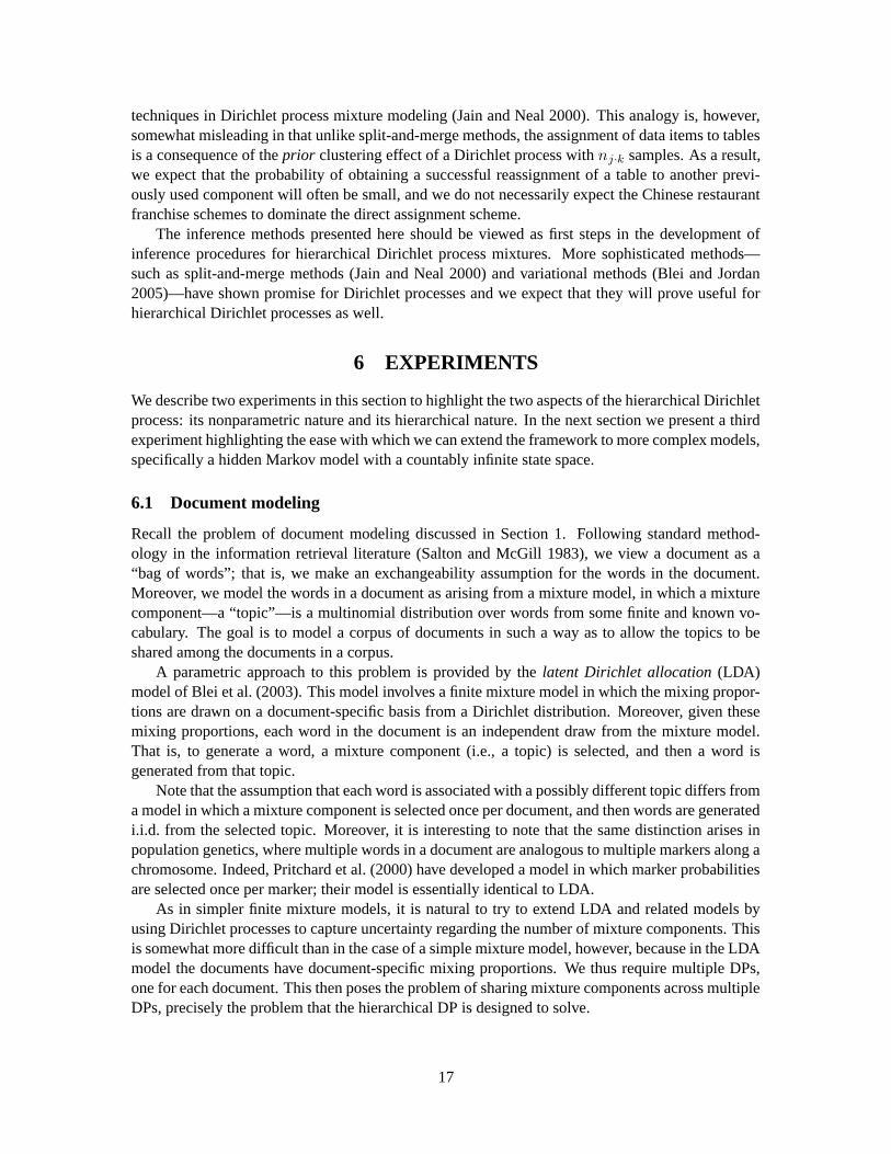
6 EXPERIMENTS

We describe two experiments in this section to highlight the two aspects of the hierarchical Dirichletprocess: its nonparametric nature and its hierarchical nature. In the next section we present a thirdexperiment highlighting the ease with which we can extend the framework to more complex models,specifically a hidden Markov model with a countably infinite state space.

6.1 Document modeling

Recall the problem of document modeling discussed in Section 1. Following standard method-ology in the information retrieval literature (Salton and McGill 1983), we view a document as a“bag of words”; that is, we make an exchangeability assumption for the words in the document.Moreover, we model the words in a document as arising from a mixture model, in which a mixturecomponent—a “topic”—is a multinomial distribution over words from some finite and known vo-cabulary. The goal is to model a corpus of documents in such a way as to allow the topics to beshared among the documents in a corpus.

A parametric approach to this problem is provided by the latent Dirichlet allocation (LDA)model of Blei et al. (2003). This model involves a finite mixture model in which the mixing propor-tions are drawn on a document-specific basis from a Dirichlet distribution. Moreover, given thesemixing proportions, each word in the document is an independent draw from the mixture model.That is, to generate a word, a mixture component (i.e., a topic) is selected, and then a word isgenerated from that topic.

Note that the assumption that each word is associated with a possibly different topic differs froma model in which a mixture component is selected once per document, and then words are generatedi.i.d. from the selected topic. Moreover, it is interesting to note that the same distinction arises inpopulation genetics, where multiple words in a document are analogous to multiple markers along achromosome. Indeed, Pritchard et al. (2000) have developed a model in which marker probabilitiesare selected once per marker; their model is essentially identical to LDA.

As in simpler finite mixture models, it is natural to try to extend LDA and related models byusing Dirichlet processes to capture uncertainty regarding the number of mixture components. Thisis somewhat more difficult than in the case of a simple mixture model, however, because in the LDAmodel the documents have document-specific mixing proportions. We thus require multiple DPs,one for each document. This then poses the problem of sharing mixture components across multipleDPs, precisely the problem that the hierarchical DP is designed to solve.

17

10 20 30 40 50 60 70 80 90 100 110 120750

800

850

900

950

1000

1050

Perp

lexi

ty

Number of LDA topics

Perplexity on test abstacts of LDA and HDP mixture

LDAHDP Mixture

61 62 63 64 65 66 67 68 69 70 71 72 730

5

10

15

Number of topics

Num

ber

of s

ampl

es

Posterior over number of topics in HDP mixture

Figure 3: (Left) Comparison of latent Dirichlet allocation and the hierarchical Dirichlet process mixture.Results are averaged over 10 runs; the error bars are one standard error. (Right) Histogram of the number oftopics for the hierarchical Dirichlet process mixture over 100 posterior samples.

The hierarchical DP extension of LDA thus takes the following form. Given an underlyingmeasure H on multinomial probability vectors, we select a random measure G0 which provides acountably infinite collection of multinomial probability vectors; these can be viewed as the set of alltopics that can be used in a given corpus. For the jth document in the corpus we sample Gj usingG0 as a base measure; this selects specific subsets of topics to be used in document j. From Gj

we then generate a document by repeatedly sampling specific multinomial probability vectors θjifrom Gj and sampling words xji with probabilities θji. The overlap among the random measuresGj implements the sharing of topics among documents.

We fit both the standard parametric LDA model and its hierarchical DP extension to a corpusof nematode biology abstracts (see http://elegans.swmed.edu/wli/cgcbib). There are 5838 abstractsin total. After removing standard stop words and words appearing fewer than 10 times, we are leftwith 476441 words in total. Following standard information retrieval methodology, the vocabularyis defined as the set of distinct words left in all abstracts; this has size 5699.

Both models were as similar as possible beyond the distinction that LDA assumes a fixed finitenumber of topics while the hierarchical Dirichlet process does not. Both models used a symmetricDirichlet distribution with parameters of 0.5 for the prior H over topic distributions. The concen-tration parameters were given vague gamma priors, γ ∼ Gamma(1, .1) and α0 ∼ Gamma(1, 1).The distribution over topics in LDA is assumed to be symmetric Dirichlet with parameters α0/Lwith L being the number of topics; γ is not used in LDA. Posterior samples were obtained using theChinese restaurant franchise sampling scheme, while the concentration parameters were sampledusing the auxiliary variable sampling scheme presented in the appendix.

We evaluated the models via 10-fold cross-validation. The evaluation metric was the perplex-ity, a standard metric in the information retrieval literature. The perplexity of a held-out abstractconsisting of words w1, . . . , wI is defined to be:

exp

(

−1

Ilog p(w1, . . . , wI |Training corpus)

)

(41)

where p(·) is the probability mass function for a given model.The results are shown in Figure 3. For LDA we evaluated the perplexity for mixture component

cardinalities ranging between 10 and 120. As seen in Figure 3 (Left), the hierarchical DP mixtureapproach—which integrates over the mixture component cardinalities—performs as well as the

18

best LDA model, doing so without any form of model selection procedure. Moreover, as shown inFigure 3 (Right), the posterior over the number of topics obtained under the hierarchical DP mixturemodel is consistent with this range of the best-fitting LDA models.

6.2 Multiple corpora

We now consider the problem of sharing clusters among the documents in multiple corpora. Weapproach this problem by extending the hierarchical Dirichlet process to a third level. A draw froma top-level DP yields the base measure for each of a set of corpus-level DPs. Draws from eachof these corpus-level DPs yield the base measures for DPs associated with the documents within acorpus. Finally, draws from the document-level DPs provide a representation of each document asa probability distribution across topics (which are distributions across words). The model allowstopics to be shared both within each corpus and between corpora.

The documents that we used for these experiments consist of articles from the proceedingsof the Neural Information Processing Systems (NIPS) conference for the years 1988-1999. Theoriginal articles are available at http://books.nips.cc; we use a preprocessed version available athttp://www.cs.utoronto.ca/∼roweis/nips. The NIPS conference deals with a range of topics coveringboth human and machine intelligence. Articles are separated into nine sections: algorithms andarchitectures (AA), applications (AP), cognitive science (CS), control and navigation (CN), imple-mentations (IM), learning theory (LT), neuroscience (NS), signal processing (SP), vision sciences(VS). (These are the sections used in the years 1995-1999. The sectioning in earlier years differedslightly; we manually relabeled sections from the earlier years to match those used in 1995-1999.)We treat these sections as “corpora,” and are interested in the pattern of sharing of topics amongthese corpora.

There were 1447 articles in total. Each article was modeled as a bag-of-words. We culledstandard stop words as well as words occurring more than 4000 or fewer than 50 times in the wholecorpus. This left us with on average slightly more than 1000 words per article.

We considered the following experimental setup. Given a set of articles from a single NIPSsection that we wish to model (the VS section in the experiments that we report below), we wish toknow whether it is of value (in terms of prediction performance) to include articles from other NIPSsections. This can be done in one of two ways: we can lump all of the articles together withoutregard for the division into sections, or we can use the hierarchical DP approach to link the sections.Thus we consider three models (see Figure 4 for graphical representations of these models):

• M1: This model ignores articles from the other sections and simply uses a hierarchical DPmixture of the kind presented in Section 6.1 to model the VS articles. This model serves asa baseline. We used γ ∼ Gamma(5, 0.1) and α0 ∼ Gamma(0.1, 0.1) as prior distributionsfor the concentration parameters.

• M2: This model incorporates articles from other sections, but ignores the distinction intosections, using a single hierarchical DP mixture model to model all of the articles. Priors ofγ ∼ Gamma(5, 0.1) and α0 ∼ Gamma(0.1, 0.1) were used.

• M3: This model takes a full hierarchical approach and models the NIPS sections as multiplecorpora, linked via the hierarchical DP mixture formalism. The model is a tree, in which theroot is a draw from a single DP for all articles, the first level is a set of draws from DPs for theNIPS sections, and the second level is set of draws from DPs for the articles within sections.Priors of γ ∼ Gamma(5, 0.1), α0 ∼ Gamma(5, 0.1), and α1 ∼ Gamma(0.1, 0.1) wereused.

19

θ

Gj

G0

Hγ

0α

Gj

VS Trainingdocuments

xji

ji

VS Testdocuments

xji

jiθ θ

Gj

G0

Hγ

0α

Gj Gj

VS Trainingdocuments

Additional trainingdocuments

xji

ji

xji

ji

VS Testdocuments

xji

jiθ θ θ

Gj

G1 G2

γ H

0α

α1

G0

Gj Gj

VS Trainingdocuments

Additional trainingdocuments

xji

ji

xji

ji

VS Testdocuments

xji

jiθ θ

M1 M2 M3

Figure 4: Three models for the NIPS data. From left to right: M1, M2 and M3.

In all models a finite and known vocabulary is assumed and the base measureH used is a symmetricDirichlet distribution with parameters of 0.5.

We conducted experiments in which a set of 80 articles were chosen uniformly at random fromone of the sections other than VS (this was done to balance the impact of different sections, whichare of different sizes). A training set of 80 articles were also chosen uniformly at random from theVS section, as were an additional set of 47 test articles distinct from the training articles. Resultsreport predictive performance on VS test articles based on a training set consisting of the 80 arti-cles in the additional section and N VS training articles where N varies between 0 and 80. Thedirect assignment sampling scheme is used, while concentration parameters are sampled using theauxiliary variable sampling scheme in the appendix.

Figure 5 (Left) presents the average predictive performance for all three models over 5 runs asthe number N of VS training articles ranged from 0 to 80. The performance is measured in termsof the perplexity of single words in the test articles given the training articles, averaged over thechoice of which additional section was used. As seen in the figure, the fully hierarchical model M3performs best, with perplexity decreasing rapidly with modest values of N . For small values of N ,the performance of M1 is quite poor, but the performance approaches that of M3 when more than 20articles are included in the VS training set. The performance of the partially-hierarchical M2 waspoorer than the fully-hierarchical M3 throughout the range of N . M2 dominated M1 for small N ,but yielded poorer performance than M1 forN greater than 14. Our interpretation is that the sharingof strength based on other articles is useful when little other information is available (small N ), butthat eventually (medium to large N ) there is crosstalk between the sections and it is preferable tomodel them separately and share strength via the hierarchy.

While the results in Figure 5 (Left) are an average over the sections, it is also of interest tosee which sections are the most beneficial in terms of enhancing the prediction of the articles inVS. Figure 5 (Right) plots the predictive performance for model M3 when given data from eachof three particular sections: LT, AA and AP. While articles in the LT section are concerned mostlywith theoretical properties of learning algorithms, those in AA are mostly concerned with modelsand methodology, and those in AP are mostly concerned with applications of learning algorithms to

20

0 10 20 30 40 50 60 70 802500

3000

3500

4000

4500

5000

5500

6000

Number of VS training documents

Perp

lexi

ty

Average perplexity over NIPS sections of 3 models

M1: additional sction ignoredM2: flat, additional sectionM3: hierarchical, additional section

0 10 20 30 40 50 60 70 802500

3000

3500

4000

4500

5000

Number of VS training documents

Perp

lexi

ty

Generalization from LT, AA, AP to VS

LTAAAP

Figure 5: (Left) Perplexity of single words in test VS articles given training articles from VS and anothersection for 3 different models. Curves shown are averaged over the other sections and 5 runs. (Right)Perplexity of test VS articles given LT, AA and AP articles respectively, using M3, averaged over 5 runs. Inboth plots, the error bars represent one standard error.

various problems. As seen in the figure, we see that predictive performance is enhanced the mostby prior exposure to articles from AP, less by articles from AA, and still less by articles from LT.Given that articles in VS tend to be concerned with the practical application of learning algorithmsto problems in computer vision, this pattern of transfer seems reasonable.

Finally, it is of interest to investigate the subject matter content of the topics discovered by thehierarchical DP model. We did so in the following experimental setup. For a given section otherthan VS (e.g., AA), we fit a model based on articles from that section. We then introduced articlesfrom the VS section and continued to fit the model, while holding the topics found from the earlierfit fixed, and recording which topics from the earlier section were allocated to words in the VSsection. Table 1 displays representations of the two most frequently occurring topics in this setup(a topic is represented by the set of words which have highest probability under that topic). Thesetopics provide qualitative confirmation of our expectations regarding the overlap between VS andother sections.

7 HIDDEN MARKOV MODELS

The simplicity of the hierarchical DP specification—the base measure for a DP is distributed as aDP—makes it straightforward to exploit the hierarchical DP as a building block in more complexmodels. In this section we demonstrate this in the case of the hidden Markov model.

Recall that a hidden Markov model (HMM) is a doubly stochastic Markov chain in which asequence of multinomial “state” variables (v1, v2, . . . , vT ) are linked via a state transition matrix,and each element yt in a sequence of “observations” (y1, y2, . . . , yT ) is drawn independently ofthe other observations conditional on vt (Rabiner 1989). This is essentially a dynamic variant of afinite mixture model, in which there is one mixture component corresponding to each value of themultinomial state. As with classical finite mixtures, it is interesting to consider replacing the finitemixture underlying the HMM with a Dirichlet process.

Note that the HMM involves not a single mixture model, but rather a set of mixture models—one for each value of the current state. That is, the “current state” vt indexes a specific row of thetransition matrix, with the probabilities in this row serving as the mixing proportions for the choice

21

Table 1: Topics shared between VS and the other NIPS sections. These topics are the most fre-quently occurring in the VS fit, under the constraint that they are associated with a significantnumber of words (greater than 2500) from the other section.

CStask representation pattern processing trained representations three process unitpatternsexamples concept similarity bayesian hypotheses generalization numbers positiveclasses hypothesis

NScells cell activity response neuron visual patterns pattern single figvisual cells cortical orientation receptive contrast spatial cortex stimulus tuning

LTsignal layer gaussian cells fig nonlinearity nonlinear rate eq celllarge examples form point see parameter consider random small optimal

AAalgorithms test approach methods based point problems form large paperdistance tangent image images transformation transformations pattern vectors convolu-tion simard

IMprocessing pattern approach architecture single shows simple based large controlmotion visual velocity flow target chip eye smooth direction optical

SPvisual images video language image pixel acoustic delta lowpass flowsignals separation signal sources source matrix blind mixing gradient eq

APapproach based trained test layer features table classification rate paperimage images face similarity pixel visual database matching facial examples

CNii tree pomdp observable strategy class stochastic history strategies densitypolicy optimal reinforcement control action states actions step problems goal

22

φ

0α

H

γ β

v

y

T

T

v1 v

y2

2

y1

v0kπ

8

k

Figure 6: A graphical representation of a hierarchical Dirichlet process hidden Markov model.

of the “next state” vt+1. Given the next state vt+1, the observation yt+1 is drawn from the mixturecomponent indexed by vt+1. Thus, to consider a nonparametric variant of the HMM which allowsan unbounded set of states, we must consider a set of DPs, one for each value of the current state.Moreover, these DPs must be linked, because we want the same set of “next states” to be reachablefrom each of the “current states.” This amounts to the requirement that the atoms associated withthe state-conditional DPs should be shared—exactly the framework of the hierarchical DP.

Thus, we can define a nonparametric hidden Markov model by simply replacing the set of con-ditional finite mixture models underlying the classical HMM with a hierarchical Dirichlet processmixture model. We refer to the resulting model as a hierarchical Dirichlet process hidden Markovmodel (HDP-HMM). The HDP-HMM provides an alternative to methods that place an explicit para-metric prior on the number of states or make use of model selection methods to select a fixed numberof states (Stolcke and Omohundro 1993).

In work that served as an inspiration for the HDP-HMM, Beal et al. (2002) discussed a modelknown as the infinite hidden Markov model, in which the number of hidden states of a hiddenMarkov model is allowed to be countably infinite. Indeed, Beal et al. (2002) defined a notion of“hierarchical Dirichlet process” for this model, but their “hierarchical Dirichlet process” is not hier-archical in the Bayesian sense—involving a distribution on the parameters of a Dirichlet process—but is instead a description of a coupled set of urn models. We briefly review this construction, andrelate it to our formulation.

Beal et al. (2002) considered the following two-level procedure for determining the transitionprobabilities of a Markov chain with an unbounded number of states. At the first level, the prob-ability of transitioning from a state u to a state v is proportional to the number of times the sametransition is observed at other time steps, while with probability proportional to α0 an “oracle” pro-cess is invoked. At this second level, the probability of transitioning to state v is proportional tothe number of times state v has been chosen by the oracle (regardless of the previous state), whilethe probability of transitioning to a novel state is proportional to γ. The intended role of the oracleis to tie together the transition models so that they have destination states in common, in much thesame way that the baseline distribution G0 ties together the group-specific mixture components inthe hierarchical Dirichlet process.

To relate this two-level urn model to the hierarchical DP framework, let us describe a represen-tation of the HDP-HMM using the stick-breaking formalism. In particular, consider the hierarchicalDirichlet process representation shown in Figure 6. The parameters in this representation have thefollowing distributions:

β | γ ∼ GEM(γ) πk | α0,β ∼ DP(α0,β) φk | H ∼ H , (42)

23

for each k = 1, 2, . . ., while for time steps t = 1, . . . , T the state and observation distributions are:

vt | vt−1, (πk)∞k=1 ∼ πvt−1

yt | vt, (φk)∞k=1 ∼ F (φvt) , (43)

where we assume for simplicity that there is a distinguished initial state v0. If we now considerthe Chinese restaurant franchise representation of this model as discussed in Section 5, it turns outthat the result is equivalent to the coupled urn model of Beal et al. (2002), hence the infinite hiddenMarkov model is an HDP-HMM.

Unfortunately, posterior inference using the Chinese restaurant franchise representation is awk-ward for this model, involving substantial bookkeeping. Indeed, Beal et al. (2002) did not presentan MCMC inference algorithm for the infinite hidden Markov model, proposing instead a heuristicapproximation to Gibbs sampling. On the other hand, both the augmented representation and di-rect assignment representations lead directly to MCMC sampling schemes that are straightforwardto implement. In the experiments reported in the following section we used the direct assignmentrepresentation.

Practical applications of hidden Markov models often consider sets of sequences, and treat thesesequences as exchangeable at the level of sequences. Thus, in applications to speech recognition, ahidden Markov model for a given word in the vocabulary is generally trained via replicates of thatword being spoken. This setup is readily accommodated within the hierarchical DP framework bysimply considering an additional level of the Bayesian hierarchy, letting a master Dirichlet processcouple each of the HDP-HMMs, each of which is a set of Dirichlet processes.

7.1 Alice in Wonderland

In this section we report experimental results for the problem of predicting strings of letters insentences taken from Lewis Carroll’s Alice’s Adventures in Wonderland, comparing the HDP-HMMto other HMM-related approaches.

Each sentence is treated as a sequence of letters and spaces (rather than as a sequence of words).There are 27 distinct symbols (26 letters and space); cases and punctuation marks are ignored.There are 20 training sentences with average length of 51 symbols, and there are 40 test sentenceswith an average length of 100. The base distribution H is a symmetric Dirichlet distribution over27 symbols with parameters 0.1. The concentration parameters γ and α0 are given Gamma(1, 1)priors.

Using the direct assignment sampling method for posterior predictive inference, we comparedthe HDD-HMM to a variety of other methods for prediction using hidden Markov models: (1) aclassical HMM using maximum likelihood (ML) parameters obtained via the Baum-Welch algo-rithm (Rabiner 1989), (2) a classical HMM using maximum a posteriori (MAP) parameters, takingthe priors to be independent, symmetric Dirichlet distributions for both the transition and emissionprobabilities, and (3) a classical HMM trained using an approximation to a full Bayesian analysis—in particular, a variational Bayesian (VB) method due to MacKay (1997) and described in detail inBeal (2003). For each of these classical HMMs, we conducted experiments for each value of thestate cardinality ranging from 1 to 60.

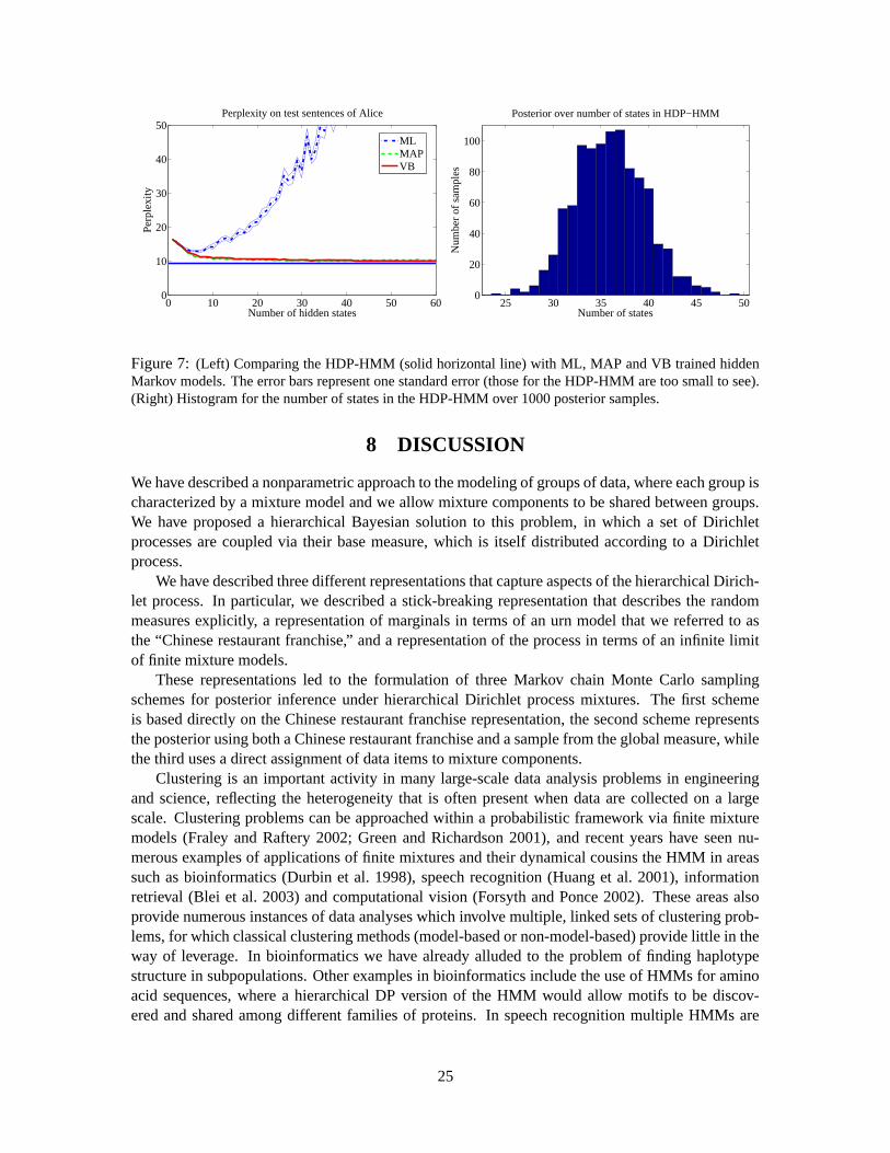
We present the perplexity on test sentences in Figure 7 (Left). For VB, the predictive probabilityis intractable to compute, so the modal setting of parameters was used. Both MAP and VB modelswere given optimal settings of the hyperparameters found using the HDP-HMM. We see that theHDP-HMM has a lower perplexity than all of the models tested for ML, MAP, and VB. Figure 7(Right) shows posterior samples of the number of states used by the HDP-HMM.

24

0 10 20 30 40 50 600

10

20

30

40

50

Number of hidden states

Perp

lexi

ty

Perplexity on test sentences of Alice

MLMAPVB

25 30 35 40 45 500

20

40

60

80

100

Number of states

Num

ber

of s

ampl

es

Posterior over number of states in HDP−HMM

Figure 7: (Left) Comparing the HDP-HMM (solid horizontal line) with ML, MAP and VB trained hiddenMarkov models. The error bars represent one standard error (those for the HDP-HMM are too small to see).(Right) Histogram for the number of states in the HDP-HMM over 1000 posterior samples.

8 DISCUSSION

We have described a nonparametric approach to the modeling of groups of data, where each group ischaracterized by a mixture model and we allow mixture components to be shared between groups.We have proposed a hierarchical Bayesian solution to this problem, in which a set of Dirichletprocesses are coupled via their base measure, which is itself distributed according to a Dirichletprocess.

We have described three different representations that capture aspects of the hierarchical Dirich-let process. In particular, we described a stick-breaking representation that describes the randommeasures explicitly, a representation of marginals in terms of an urn model that we referred to asthe “Chinese restaurant franchise,” and a representation of the process in terms of an infinite limitof finite mixture models.

These representations led to the formulation of three Markov chain Monte Carlo samplingschemes for posterior inference under hierarchical Dirichlet process mixtures. The first schemeis based directly on the Chinese restaurant franchise representation, the second scheme representsthe posterior using both a Chinese restaurant franchise and a sample from the global measure, whilethe third uses a direct assignment of data items to mixture components.

Clustering is an important activity in many large-scale data analysis problems in engineeringand science, reflecting the heterogeneity that is often present when data are collected on a largescale. Clustering problems can be approached within a probabilistic framework via finite mixturemodels (Fraley and Raftery 2002; Green and Richardson 2001), and recent years have seen nu-merous examples of applications of finite mixtures and their dynamical cousins the HMM in areassuch as bioinformatics (Durbin et al. 1998), speech recognition (Huang et al. 2001), informationretrieval (Blei et al. 2003) and computational vision (Forsyth and Ponce 2002). These areas alsoprovide numerous instances of data analyses which involve multiple, linked sets of clustering prob-lems, for which classical clustering methods (model-based or non-model-based) provide little in theway of leverage. In bioinformatics we have already alluded to the problem of finding haplotypestructure in subpopulations. Other examples in bioinformatics include the use of HMMs for aminoacid sequences, where a hierarchical DP version of the HMM would allow motifs to be discov-ered and shared among different families of proteins. In speech recognition multiple HMMs are

25

already widely used, in the form of word-specific and speaker-specific models, and adhoc meth-ods are generally used to share statistical strength among models. We have discussed examplesof grouped data in information retrieval; other examples include problems in which groups are in-dexed by author or by language. Finally, computational vision and robotics problems often involvesets of descriptors or objects that are arranged in a taxonomy. Examples such as these, in whichthere is substantial uncertainty regarding appropriate numbers of clusters, and in which the sharingof statistical strength among groups is natural and desirable, suggest that the hierarchical nonpara-metric Bayesian approach to clustering presented here may provide a generally useful extension ofmodel-based clustering.

A Posterior sampling for concentration parameters

MCMC samples from the posterior distributions for the concentration parameters γ and α0 of thehierarchical Dirichlet process can be obtained using straightforward extensions of analogous tech-niques for Dirichlet processes. Let the number of observed groups be equal to J , with nj·· observa-tions in the j th group. Consider the Chinese restaurant franchise representation. The concentrationparameter α0 governs the distribution of the number of ψjt’s in each mixture. As noted in Sec-tion 5.3 this is given by:

p(m1·, . . . ,mJ ·|α0, n1··, . . . , nJ ··) =

J∏

j=1

s(nj··,mj·)αmj·

0

Γ(α0)

Γ(α0 + nj··). (44)

Further, α0 does not govern other aspects of the joint distribution, hence (44) along with the priorfor α0 is sufficient to derive MCMC updates for α0 given all other variables.

In the case of a single mixture model (J = 1), Escobar and West (1995) proposed a gamma priorand derived an auxiliary variable update for α0, while Rasmussen (2000) observed that (44) is log-concave in log(α0) and proposed using adaptive rejection sampling instead. The adaptive rejectionsampler of Rasmussen (2000) can be directly applied to the case J > 1 since the conditionaldistribution of log(α0) is still log-concave. The auxiliary variable method of Escobar and West(1995) requires a slight modification for the case J > 1. Assume that the prior for α0 is a gammadistribution with parameters a and b. For each j we can write

Γ(α0)

Γ(α0 + nj··)=

1

Γ(nj··)

∫ 1

0wα0

j (1 − wj)nj··−1

(

1 +nj··α0

)

dwj . (45)

We define auxiliary variables w = (wj)Jj=1 and s = (sj)

Jj=1 where each wj is a variable taking on

values in [0, 1], and each sj is a binary {0, 1} variable, and define the following distribution:

q(α0,w, s) ∝ αa−1+m··

0 e−α0bJ∏

j=1

wα0

j (1 − wj)nj··−1

(

nj··α0

)sj

. (46)

Now marginalizing q to α0 gives the desired conditional distribution for α0. Hence q defines anauxiliary variable sampling scheme for α0. Given w and s we have:

q(α0|w, s) ∝ αa−1+m··−

∑Jj=1

sj

0 e−α0(b−∑J

j=1logwj) , (47)

26

which is a gamma distribution with parameters a+m··−∑J

j=1 sj and b−∑J

j=1 logwj . Given α0,the wj and sj are conditionally independent, with distributions:

q(wj |α0) ∝ wα0

j (1 − wj)nj··−1 (48)

q(sj |α0) ∝

(

nj··α0

)sj

, (49)

which are beta and binomial distributions respectively. This completes the auxiliary variable sam-pling scheme for α0. We prefer the auxiliary variable sampling scheme as it is easier to implementand typically mixes quickly (within 20 iterations).

Given the total number m·· of ψjt’s, the concentration parameter γ governs the distribution overthe number of components K:

p(K|γ,m··) = s(m··,K)γKΓ(γ)

Γ(γ +m··). (50)

Again other variables are independent of γ given m·· and K, hence we may apply the techniques ofEscobar and West (1995) or Rasmussen (2000) directly to sampling γ.

Acknowledgments

We wish to acknowledge helpful discussions with Lancelot James. We also wish to acknowledgesupport from Intel Corporation, Microsoft Research, and a grant from Darpa in support of the CALOprogram.

References

Aldous, D. (1985), “Exchangeability and Related Topics,” in Ecole d’Ete de Probabilites de Saint-Flour XIII–1983, Springer, Berlin, pp. 1–198.

Antoniak, C. (1974), “Mixtures of Dirichlet Processes with Applications to Bayesian NonparametricProblems,” Annals of Statistics, 2(6), pp. 1152–1174.

Beal, M. (2003), “Variational Algorithms for Approximate Bayesian Inference,” Ph.D. thesis,Gatsby Computational Neuroscience Unit, University College London.

Beal, M. J., Ghahramani, Z., and Rasmussen, C. (2002), “The Infinite Hidden Markov Model,” inT. G. Dietterich, S. Becker, and Z. Ghahramani (eds.) Advances in Neural Information ProcessingSystems, Cambridge, MA: MIT Press, vol. 14, pp. 577–584.

Blackwell, D. and MacQueen, J. (1973), “Ferguson Distributions via Polya Urn Schemes,” Annalsof Statistics, 1, pp. 353–355.

Blei, D., Jordan, M., and Ng, A. (2003), “Hierarchical Bayesian Models for Applications in Infor-mation Retrieval,” in Bayesian Statistics, vol. 7, pp. 25–44.

Blei, D. M. and Jordan, M. I. (2005), “Variational methods for Dirichlet process mixtures,” BayesianAnalysis, 1, pp. 121–144.

27

Carota, C. and Parmigiani, G. (2002), “Semiparametric Regression for Count Data,” Biometrika,89(2), pp. 265–281.

Cifarelli, D. and Regazzini, E. (1978), “Problemi Statistici Non Parametrici in Condizioni di Scam-biabilita Parziale e Impiego di Medie Associative,” Tech. rep., Quaderni Istituto Matematica Fi-nanziaria dell’Universita di Torino.

De Iorio, M., Muller, P., and Rosner, G. (2004), “An ANOVA Model for Dependent Random Mea-sures,” Journal of the American Statistical Association, 99(465), pp. 205–215.

Durbin, R., Eddy, S., Krogh, A., and Mitchison, G. (1998), Biological Sequence Analysis, Cam-bridge, UK: Cambridge University Press.

Escobar, M. and West, M. (1995), “Bayesian Density Estimation and Inference Using Mixtures,”Journal of the American Statistical Association, 90, pp. 577–588.

Ferguson, T. (1973), “A Bayesian Analysis of Some Nonparametric Problems,” Annals of Statistics,1(2), pp. 209–230.

Fong, D., Pammer, S., Arnold, S., and Bolton, G. (2002), “Reanalyzing Ultimatum Bargaining—Comparing Nondecreasing Curves Without Shape Constraints,” Journal of Business and Eco-nomic Statistics, 20, pp. 423–440.

Forsyth, D. A. and Ponce, J. (2002), Computer Vision—A Modern Approach, Upper Saddle River,NJ: Prentice-Hall.

Fraley, C. and Raftery, A. E. (2002), “Model-Based Clustering, Discriminant Analysis, and DensityEstimation,” Journal of the American Statistical Association, 97, pp. 611–631.

Gabriel, S. et al. (2002), “The Structure of Haplotype Blocks in the Human Genome,” Science, 296,pp. 2225–2229.

Green, P. and Richardson, S. (2001), “Modelling Heterogeneity with and without the DirichletProcess,” Scandinavian Journal of Statistics, 28, pp. 355–377.

Huang, X., Acero, A., and Hon, H.-W. (2001), Spoken Language Processing, Upper Saddle River,NJ: Prentice-Hall.

Ishwaran, H. and James, L. (2004), “Computational Methods for Multiplicative Intensity Modelsusing Weighted Gamma Processes: Proportional Hazards, Marked Point Processes and PanelCount Data,” Journal of the American Statistical Association, 99, pp. 175–190.

Ishwaran, H. and Zarepour, M. (2002), “Exact and Approximate Sum-Representations for theDirichlet Process,” Canadian Journal of Statistics, 30, pp. 269–283.

Jain, S. and Neal, R. (2000), “A Split-Merge Markov Chain Monte Carlo Procedure for the DirichletProcess Mixture Model,” Tech. Rep. 2003, Department of Statistics, University of Toronto.

Kleinman, K. and Ibrahim, J. (1998), “A Semi-parametric Bayesian Approach to Generalized LinearMixed Models,” Statistics in Medicine, 17, pp. 2579–2596.

MacEachern, S. (1999), “Dependent Nonparametric Processes,” in Proceedings of the Section onBayesian Statistical Science, American Statistical Association.

28

MacEachern, S., Kottas, A., and Gelfand, A. (2001), “Spatial Nonparametric Bayesian Models,”Tech. Rep. 01-10, Institute of Statistics and Decision Sciences, Duke University.

MacEachern, S. and Muller, P. (1998), “Estimating Mixture of Dirichlet Process Models,” Journalof Computational and Graphical Statistics, 7, pp. 223–238.

MacKay, D. and Peto, L. (1994), “A Hierarchical Dirichlet Language Model,” Natural LanguageEngineering.

MacKay, D. J. C. (1997), “Ensemble Learning for Hidden Markov Models,” Tech. rep., CavendishLaboratory, University of Cambridge.

Mallick, B. and Walker, S. (1997), “Combining Information from Several Experiments with Non-parametric Priors,” Biometrika, 84, pp. 697–706.

Muliere, P. and Petrone, S. (1993), “A Bayesian Predictive Approach to Sequential Search for anOptimal Dose: Parametric and Nonparametric Models,” Journal of the Italian Statistical Society,2, pp. 349–364.

Muller, P., Quintana, F., and Rosner, G. (2004), “A Method for Combining Inference Across RelatedNonparametric Bayesian Models,” Journal of the Royal Statistical Society, 66, pp. 735–749.

Neal, R. (1992), “Bayesian Mixture Modeling,” in Proceedings of the Workshop on Maximum En-tropy and Bayesian Methods of Statistical Analysis, vol. 11, pp. 197–211.

—— (2000), “Markov Chain Sampling Methods for Dirichlet Process Mixture Models,” Journal ofComputational and Graphical Statistics, 9, pp. 249–265.

Pitman, J. (1996), “Random discrete distributions invariant under size-biased permutation,” Ad-vances in Applied Probability, 28, pp. 525–539.

—— (2002a), “Combinatorial Stochastic Processes,” Tech. Rep. 621, Department of Statistics, Uni-versity of California at Berkeley, lecture notes for St. Flour Summer School.

—— (2002b), “Poisson-Dirichlet and GEM invariant distributions for split-and-merge transforma-tions of an interval partition,” Combinatorics, Probability and Computing, 11, pp. 501–514.

Pritchard, J., Stephens, M., and Donnelly, P. (2000), “Inference of Population Structure using Mul-tilocus Genotype Data,” Genetics, 155, pp. 945–959.

Rabiner, L. (1989), “A Tutorial on Hidden Markov Models and Selected Applications in SpeechRecognition,” Proceedings of the IEEE, 77, pp. 257–285.

Rasmussen, C. (2000), “The Infinite Gaussian Mixture Model,” in S. Solla, T. Leen, and K.-R.Muller (eds.) Advances in Neural Information Processing Systems, Cambridge, MA: MIT Press,vol. 12.

Salton, G. and McGill, M. (1983), An Introduction to Modern Information Retrieval, New York:McGraw-Hill.

Sethuraman, J. (1994), “A Constructive Definition of Dirichlet Priors,” Statistica Sinica, 4, pp. 639–650.

29

Stephens, M., Smith, N., and Donnelly, P. (2001), “A New Statistical Method for Haplotype Recon-struction from Population Data,” American Journal of Human Genetics, 68, pp. 978–989.

Stolcke, A. and Omohundro, S. (1993), “Hidden Markov Model Induction by Bayesian ModelMerging,” in C. Giles, S. Hanson, and J. Cowan (eds.) Advances in Neural Information ProcessingSystems, San Mateo CA: Morgan Kaufmann, vol. 5, pp. 11–18.

Tomlinson, G. (1998), “Analysis of Densities,” Ph.D. thesis, Department of Public Health Sciences,University of Toronto.

Tomlinson, G. and Escobar, M. (2003), “Analysis of Densities,” Tech. rep., Department of PublicHealth Sciences, University of Toronto.

30