Hierarchical Bayes Models -...
10
Bayesian Inference 1/18/06 36 Hierarchical Bayes Models • The hierarchical Bayes idea has become very important in recent years • It allows us to entertain a much richer class of models that can better capture our statistical understanding of the problem • With the advent of MCMC, it has become possible to do the calculations on these much more complex models, thus rendering the hierarchical Bayes approach much more practical Bayesian Inference 1/18/06 37 Hierarchical Bayes Models • Nonhierarchical models have a very simple structure, e.g., • This can be represented by a DAG (Directed Acyclic Graph), which diagrams the dependencies of each variable on others. Since x is stochastically dependent on X and ! in the above model, we get the following DAG: p( X, " | x ) # p( x | X, " )$ ( X )$ ( " ) x X ! Bayesian Inference 1/18/06 38 Hierarchical Bayes Models • The basic idea in a hierarchical model is that when you look at the likelihood function, and decide on the right priors, it may be appropriate to use priors that themselves depend on other parameters not mentioned in the likelihood. These parameters themselves will require priors, which themselves may (or may not) depend on new parameters. Eventually the process terminates when we no longer introduce new parameters Bayesian Inference 1/18/06 39 Hierarchical Bayes Models • Thus we might have something like • To which we would associate the DAG shown in the figure. The new bits in red represents the new hierarchical structure (W and V are not part of the likelihood) p( X, " , W , V , Z | x ) # p( x | X, " )$ ( X | W , V )$ ( W )$ ( V )$ ( " | Z )$ ( Z ) x X W V ! Z
Transcript of Hierarchical Bayes Models -...

Bayesian Inference 1/18/06 36
Hierarchical Bayes Models
• The hierarchical Bayes idea has become very important in
recent years
• It allows us to entertain a much richer class of models that
can better capture our statistical understanding of the
problem
• With the advent of MCMC, it has become possible to do
the calculations on these much more complex models,
thus rendering the hierarchical Bayes approach much
more practical
Bayesian Inference 1/18/06 37
Hierarchical Bayes Models
• Nonhierarchical models have a very simple structure, e.g.,
• This can be represented by a DAG (Directed Acyclic
Graph), which diagrams the dependencies of each variable
on others. Since x is stochastically dependent on X and !
in the above model, we get the following DAG:
!
p(X," | x)# p(x | X," )$(X)$(" )
x
X !
Bayesian Inference 1/18/06 38
Hierarchical Bayes Models
• The basic idea in a hierarchical model is that when you
look at the likelihood function, and decide on the right
priors, it may be appropriate to use priors that themselves
depend on other parameters not mentioned in the
likelihood. These parameters themselves will require
priors, which themselves may (or may not) depend on new
parameters. Eventually the process terminates when we no
longer introduce new parameters
Bayesian Inference 1/18/06 39
Hierarchical Bayes Models
• Thus we might have something like
• To which we would associate the DAG shown in the
figure. The new bits in red represents the new hierarchical
structure (W and V are not part of the likelihood)!
p(X," ,W ,V ,Z | x)# p(x | X," )$(X |W ,V )$(W )$(V )$(" | Z )$(Z )
x
X
W
V
!
Z

Bayesian Inference 1/18/06 40
Normal Hierarchical Model
• Consider the case of measuring the metallicity of a class
objects. We can expect that the measured metallicity
varies from star to star for two reasons: (1) measurement
error and (2) intrinsic (“cosmic”) scatter from object to
object.
• Our aim is to estimate the metallicity of the class, as well
as the individual metallicity of each star in the sample
Bayesian Inference 1/18/06 41
Normal Hierarchical Model
• Thus we postulate the following model
!
xi~ N("
i,#
i
2), where #
i
2 is known
"i~ N (µ,$ 2
)
µ ~ flat
$ ~ flat on (0,%)
Bayesian Inference 1/18/06 42
Normal Hierarchical Model
• The DAG corresponding to this model is
x
"
µ #
!
xi~ N("
i,#
i
2), where #
i
2 is known
"i~ N (µ,$ 2
)
µ ~ flat
$ ~ flat on (0,%)
Bayesian Inference 1/18/06 43
Normal Hierarchical Model
• Writing down the posterior probability explicitly we see
that
• Routine completion of the square in the first term shows
that we can sample Gibbs on µ using
where is the mean of the "’s
!
p(",µ,# | x)$1
# Nexp %
1
2# 2(µ %"i )
2&
' (
)
* +
i=1
N
,
- exp %1
2. i
2("i % xi )
2&
' (
)
* +
i=1
N
,
!
µ | x,",# ~ N(" ,# 2 /N )
!
"
Bayesian Inference 1/18/06 44
Normal Hierarchical Model
• Compare the formula with the code below:
!
µ | x,",# ~ N(" ,# 2 /N )
mu = rnorm(1,mean(theta),tau/sqrt(N))
Bayesian Inference 1/18/06 45
Normal Hierarchical Model
• Writing down the posterior probability explicitly we see
that
• Similarly, we can sample Gibbs on # using
where!
p(",µ,# | x)$1
# Nexp %
1
2# 2(µ %"i )
2&
' (
)
* +
i=1
N
,
- exp %1
2. i
2("i % xi )
2&
' (
)
* +
i=1
N
,
!
" | x,# ~ InverseChisquare(S,N $1)
!
S = (µ "#i)2
i=1
N
$
Bayesian Inference 1/18/06 46
Normal Hierarchical Model
• Compare the code with the formula:
!
" | x,# ~ InverseChisquare(S,N $1)
!
S = (µ "#i)2
i=1
N
$
tau = sqrt(sum((mu-theta)^2)/
rchisq(1,N-1))
Bayesian Inference 1/18/06 47
Normal Hierarchical Model
• Writing down the posterior probability explicitly we see
that
• By completing the square of the terms involving the
individual "i, we find that we can also sample the
individual "i:!
p(",µ,# | x)$1
# Nexp %
1
2# 2(µ %"i )
2&
' (
)
* +
i=1
N
,
- exp %1
2. i
2("i % xi )
2&
' (
)
* +
i=1
N
,
!
"i| x,µ,# ~ N(a
i, s
i
2)

Bayesian Inference 1/18/06 48
Normal Hierarchical Model
• Where
• Thus we are using a mean ai that is a weighted mean of
the observation xi and the group mean µ: The "i will
“shrink” towards the group mean. This is very typical in
hierarchical models. The variance is the usual variance for
a weighted mean.
!
ai=xi/"
i
2 + µ /# 2
1/"i
2 +1/# 2,
1
si
2=1
"i
2+1
# 2
Bayesian Inference 1/18/06 49
Normal Hierarchical Model
• Again, compare formula and code:
• Loops are inefficient in R; this is much faster than a loop
!
"i| x,µ,# ~ N(a
i, s
i
2)
!
ai=xi/"
i
2 + µ /# 2
1/"i
2 +1/# 2,
1
si
2=1
"i
2+1
# 2
S = 1/(1/sigma^2+1/tau^2)
a = (X/sigma^2+mu/tau^2)*S
theta = rnorm(N,a,sqrt(S))
Bayesian Inference 1/18/06 50
Normal Hierarchical Model
• The data are taken from a baseball example (Efron and
Morris) quoted in Peter Lee’s book Bayesian Analysis,
Second Edition.Early Season EM Estimator Late Season
Clemente 0.400 0.290 0.346
F Robinson 0.378 0.286 0.298
F Howard 0.356 0.281 0.276
Johnstone 0.333 0.277 0.222
Berry 0.311 0.273 0.273
Spencer 0.311 0.273 0.270
Kessinger 0.289 0.268 0.263
L. Alvardo 0.267 0.264 0.210
Santo 0.244 0.259 0.269
Swoboda 0.244 0.259 0.230
Unser 0.222 0.254 0.264
Williams 0.222 0.254 0.256
Scott 0.222 0.254 0.303
Petrocelli 0.222 0.254 0.264
E Rodriguez 0.222 0.254 0.226
Campaneris 0.200 0.249 0.285
Munson 0.178 0.244 0.316
Alvis 0.156 0.239 0.200
Bayesian Inference 1/18/06 51
Example: RR Lyrae Statistical Parallax
• Here’s a more complicated astronomical example that
illustrates the power of the hierarchical Bayes idea. We
consider the problem of determining the absolute
magnitude of RR Lyrae stars using proper motion and
radial velocity data
Bayesian Inference 1/18/06 52
Example: RR Lyrae Statistical Parallax
• Our data are the proper motions µ , the radial velocities & ,and the apparent magnitudes m of the stars, the latterassumed measured with negligible error.
• The proper motions are related to the cross-trackvelocities by multiplying the former by the distance s tothe star:
By assuming that the proper motions and radial velocitiesare characterized by the same kinematical parameters, wecan (statistically) infer s and then the absolute magnitudeM of the star through the well-known relationship:
!
sµ"V#
!
s =100.2(m"M +5)
Bayesian Inference 1/18/06 53
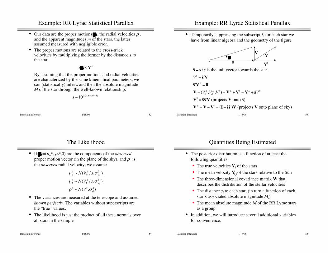
Example: RR Lyrae Statistical Parallax
• Temporarily suppressing the subscript i, for each star we
have from linear algebra and the geometry of the figure
!
ˆ s = s / s is the unit vector towards the star,
V||= ˆ " s V
ˆ " s V#
= 0
V = (V$#,V%
#,V || ) = V#
+ V||= V
#+ ˆ s V
||
V||= ˆ s ̂ " s V (projects V onto ˆ s )
V#
= V &V||= (I& ˆ s ̂ " s )V (projects V onto plane of sky)
!
V"
!
V||
V
!
µ
s
Bayesian Inference 1/18/06 54
The Likelihood
• If µo=(µ$o, µ%
o,0) are the components of the observed
proper motion vector (in the plane of the sky), and &o is
the observed radial velocity, we assume
• The variances are measured at the telescope and assumed
known perfectly. The variables without superscripts are
the “true” values.
• The likelihood is just the product of all these normals over
all stars in the sample!
µ"
o~ N (V"
#/ s,$ µ%
2)
µ%
o~ N(V%
#/ s,$ µ%
2)
&o ~ N(V ||,$&
2)
Bayesian Inference 1/18/06 55
Quantities Being Estimated
• The posterior distribution is a function of at least the
following quantities:
• The true velocities Vi of the stars
• The mean velocity V0
of the stars relative to the Sun
• The three-dimensional covariance matrix W that
describes the distribution of the stellar velocities
• The distance si to each star, (in turn a function of each
star’s associated absolute magnitude Mi)
• The mean absolute magnitude M of the RR Lyrae stars
as a group
• In addition, we will introduce several additional variables
for convenience.

Bayesian Inference 1/18/06 56
Priors Defining the Hierarchical Model
• The priors on the Vi are assigned by assuming that the
velocities of the individual stars are drawn from a (three-
dimensional) multivariate normal distribution:
• We choose an improper flat prior on V0, the mean velocity
of the RR Lyrae stars relative to the velocity of the Sun!
Vi|V
0,W ~ N(V
0,W)
Bayesian Inference 1/18/06 57
Priors Defining the Hierarchical Model
• The prior on W requires some care. One wants a proper
posterior distribution (flat priors are improper, for
example, but there is no problem if the posterior
distribution is proper)
• To satisfy this demand, while maintaining a reasonably
noncommittal (vague) prior, we chose a “hierarchical
independence Jeffreys prior” on W, which for a three-
dimensional distribution implies
!
"(W)#| $I+W |%2
Bayesian Inference 1/18/06 58
Priors Defining the Hierarchical Model
• The distances si are related to the Mi and M by an exact
(defined) relationship:
• We introduce new variables Ui=Mi–M, because
preliminary calculations indicated that sampling would be
more efficient on the variables Ui (the Mi are highly
correlated with each other and with M, but the Ui are not).
Therefore we write
!
si
=100.2(m
i"M
i+5)
!
si
=100.2(m
i"M "U
i+5)
Bayesian Inference 1/18/06 59
Priors Defining the Hierarchical Model
• Illustrating the correlation between M and one of the Mi
(doesn’t look bad but there are hundreds of stars in the
sample, which exacerbates the problem)

Bayesian Inference 1/18/06 60
Priors Defining the Hierarchical Model
• Illustrating low correlation between M and one of the Ui
Bayesian Inference 1/18/06 61
Priors Defining the Hierarchical Model
• Illustrating low correlation between the various Ui
Bayesian Inference 1/18/06 62
Priors Defining the Hierarchical Model
• We choose a flat prior on M (we have also tried a
somewhat informative prior based on known data with not
much change).
• Evidence indicates a “cosmic scatter” of about 0.15
magnitudes in Mi. Thus a prior on Ui of the form
seems appropriate.
!
Ui~ N(0,(0.15)
2)
Bayesian Inference 1/18/06 63
DAG Describing Hierarchical Model
• The following DAG is a simplified description of the
structure of the hierarchical model
V W
ViMUi
µi,!i

Bayesian Inference 1/18/06 64
DAG Describing Hierarchical Model
• The following DAG shows the structure of the
hierarchical model in more detail
Bayesian Inference 1/18/06 65
Sampling Strategy
• We can use Gibbs sampling to sample on V0
where N is the number of stars in our sample and
!
V0| {V
i},W ~ N(V ,W /N )
!
V =1
NV
i"
Bayesian Inference 1/18/06 66
Sampling Strategy
• We can also use Gibbs sampling to sample on W;
however, we cannot generate W directly, but instead use a
rejection sampling scheme. Generate a candidate W* using
where
• Then accept or reject the candidate with probability
• Repeat until successful. This scheme is very efficient for
large degrees of freedom.
!
W*| {Vi},V0 ~ InverseWishart(T,df = N )
!
T = (Vi"V
0)# (V
i"V
0$ )
!
|W*|2/ | I+W
*|2
Bayesian Inference 1/18/06 67
Sampling Strategy
• We can also use Gibbs sampling to sample on W;
however, we cannot generate W directly, but instead use a
rejection sampling scheme. Generate a candidate W* using
where
• Then accept or reject the candidate with probability
• Repeat until successful. This scheme is very efficient for
large degrees of freedom.
!
W*| {Vi},V0 ~ InverseWishart(T,df = N )
!
T = (Vi"V
0)# (V
i"V
0$ )
!
|W*|2/ | I+W
*|2
Inverse Wishart is a multivariate
version of inverse chi-square
Bayesian Inference 1/18/06 68
Sampling Strategy
• Vi can be sampled in a Gibbs step; it involves data on the
individual stars as well as the general velocity distribution,
and the covariance matrix Si of the velocities of the
individual stars depends on si because of the relation
• Omitting the algebraic details, the resulting sampling
scheme is
where
!
sµ =V"
!
Vi~ N(u
i,Z
i)
Zi= (S
i
"1 + Wi
"1)"1
ui= Z
i(S
i
"1Vi
o + W"1
V0)
Vi
o = siµi
o + ˆ s i#i
o
Bayesian Inference 1/18/06 69
Sampling Strategy
• We sample the Ui using a Metropolis-Hastings step. Our
proposal is Ui* ~ N(Ui, w) with an appropriate w, adjusted
for good mixing. Recalling that si is a function of Ui, the
conditional distribution is proportional to
with the informative prior on Ui we described earlier,
!
si
2N(s
iµi+ ˆ s
iVi
||"V
0,W)
!
Ui~ N(0,(0.15)
2)
Bayesian Inference 1/18/06 70
Sampling Strategy
• We sample on M using a Metropolis-Hastings step. Our
proposal for M* is a t distribution centered on M with an
appropriate choice of degrees of freedom and variance,
adjusted for good mixing. Recalling that si is a function of
M, the conditional is proportional to
with a prior on M that may or may not be informative (as
discussed earlier).
• We found that dof=10 and variance=0.01 on the t proposal
distribution mixed well.
!
si
2N(s
iµi+ ˆ s
iVi
|| "V0,W)#
Bayesian Inference 1/18/06 71
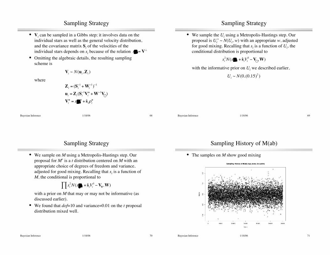
Sampling History of M(ab)
• The samples on M show good mixing

Bayesian Inference 1/18/06 72
Marginal Density of M(ab)
• Plotting a smoothed histogram of M displays the posteror
marginal distribution of M
Bayesian Inference 1/18/06 73
Marginal Density of M(c)
• The same, for the overtone pulsators


![Supervised Classification of Multi-sensor and Multi …€¦ · · 2018-04-17joint probability density functions into a hierarchical Markovian model based on ... [10], on the Bayes](https://static.fdocuments.in/doc/165x107/5ae4048b7f8b9a097a8ee2cf/supervised-classification-of-multi-sensor-and-multi-2018-04-17joint-probability.jpg)