Hierarchical Animal Movement Models for Population-Level … · Population-Level Inference for...

Population-Level Inference for Animal Movement

Hierarchical Animal Movement Models forPopulation-Level Inference

Mevin B. Hootena∗ Frances E. Budermanb, Brian M. Brostb,

Ephraim M. Hanksc, and Jacob S. Ivand

Summary: New methods for modeling animal movement based on telemetry data are developed regularly.

With advances in telemetry capabilities, animal movement models are becoming increasingly sophisticated.

Despite a need for population-level inference, animal movement models are still predominantly developed for

individual-level inference. Most efforts to upscale the inference to the population-level are either post hoc or

complicated enough that only the developer can implement the model. Hierarchical Bayesian models provide

an ideal platform for the development of population-level animal movement models but can be challenging

to fit due to computational limitations or extensive tuning required. We propose a two-stage procedure

for fitting hierarchical animal movement models to telemetry data. The two-stage approach is statistically

rigorous and allows one to fit individual-level movement models separately, then resample them using a

secondary MCMC algorithm. The primary advantages of the two-stage approach are that the first stage is

easily parallelizable and the second stage is completely unsupervised, allowing for a completely automated

fitting procedure in many cases. We demonstrate the two-stage procedure with two applications of animal

movement models. The first application involves a spatial point process approach to modeling telemetry data

and the second involves a more complicated continuous-time discrete-space animal movement model. We fit

these models to simulated data and real telemetry data arising from a population of monitored Canada lynx

in Colorado, USA.

Keywords: Hierarchical model, resource selection model, spatial statistics, telemetry data, trajectories.

aU.S. Geological Survey, Colorado Cooperative Fish and Wildlife Research Unit; Departments of Fish, Wildlife, & Conservation

Biology and Statistics, Colorado State University, Fort Collins, CO 80523bDepartment of Fish, Wildlife, and Conservation Biology, Colorado State UniversitycDepartment of Statistics, Pennsylvania State UniversitydColorado Parks and Wildlife

∗Correspondence to: M.B. Hooten, E-mail: [email protected]

arX

iv:1

606.

0958

5v1

[st

at.M

E]

30

Jun

2016

M.B. Hooten et al.

1. INTRODUCTION

The field of movement ecology is booming, in large part, because of the increased availability

of telemetry data sources (Cagnacci et al. 2010). Contemporary telemetry data are acquired

via satellite communication devices affixed to individual animals. These devices often collect

many types of data, but most studies are focused on the position data, primarily to learn

about environmental influences on individual-level movement. Many new statistical models

for animal trajectories have been proposed in recent years and they vary in form depending

on the motivation for the project and type of inference desired (Hooten et al. In Press). For

example, most individual-based statistical models for telemetry data fall into one of three

classes: point process models, discrete-time models, or continuous-time models, with each

being appropriate in certain settings (McClintock et al. 2014).

Statistical inference arising from fitting animal movement models to telemetry data

is sometimes focused on the individual level. For example, a movement ecologist might

ask how a specific individual animal responded to environmental cues while migrating

between summer and winter home ranges (e.g., Hooten et al. 2010a). However, many

animal movement studies are concerned with population-level inference. That is, for several

individuals, is there evidence of consistent behavioral responses to environmental variables?

To obtain population-level inference, the well-accepted approach is to use a hierarchical

model with random effects for individuals that are pooled at the population-level. For

2


example, consider the Bayesian hierarchical model

yj ∼ [yj|βj,θj] , (1)

βj ∼ [βj|µβ,Σβ] , (2)

µβ ∼ [µβ] , (3)

Σ−1β ∼ [Σ−1

β ] , (4)

θj ∼ [θj] , (5)

where yj are measurements associated with each individual j (j = 1, . . . , J) and we use

‘[. . .]’ to denote a probability distribution or mass/density function as necessary (Gelfand and

Smith 1990). The priors in (3)–(5) are for the auxiliary data-level parameters θj, population-

level coefficients µβ, and precision matrix Σ−1β , forming the familiar three-level hierarchical

model (Berliner 1996). The hierarchical model in (1)–(5) provides a straightforward and

intuitive means for obtaining inference for µβ, which is the ultimate goal of many animal

movement studies. Similar hierarchical models have become popular, and now standard, tools

for obtaining upscaled inference in many other fields such as atmospheric science (Cressie

and Wikle 2011), ecology (Hobbs and Hooten 2015), and sociology (Gelman and Hill 2006).

The complexity of modern animal movement models makes implementation challenging.

Furthermore, increases in the quantity of data resulting from newer telemetry devices has

outpaced computational methods for fitting animal movement models. Animal ecologists

may wish to extend individual-level models to provide statistically rigorous population-

level inference, but, in many cases, the algorithms required to fit such models become

prohibitively challenging to program or are too slow in settings with large data sets and/or

many individuals. For example, Hanks et al. (2011) performed a post hoc meta-analysis to

obtain population-level inference for northern fur seals (Callorhinus ursinus) because the

implementation of a full hierarchical movement model was not computationally feasible.

3

M.B. Hooten et al.

Furthermore, in the Bayesian setting, Markov Chain Monte Carlo (MCMC) algorithms for

most animal movement models require tuning from the user due to lack of conjugacy. In cases

where data sets from tens or hundreds of individuals are available, it may not be feasible to

tune individual-level Metropolis-Hastings updates for all parameters.

We present a statistically rigorous two-stage procedure for economizing hierarchical animal

movement models to provide exact population-level inference using a sequence of algorithms

that are fast, stable, and require little or no tuning by the user. Our approach is simple.

First, we fit individual-level models (1) independently using a preferred stochastic sampling

algorithm. Independent model fits in the first stage allow for parallel processing, leading to an

improvement in computational efficiency that scales with the number of processors. Second,

we obtain exact population-level inference using a secondary MCMC algorithm that requires

no tuning. The secondary algorithm is based on a little-known technique for Bayesian meta-

analysis proposed by Lunn et al. (2013). We found that our two-stage procedure provides

substantial computational improvements in both speed and ease of use in cases with large

data sets and/or complicated data models.

In what follows, we present a general two-stage procedure for fitting a broad class of

hierarchical animal movement models. We then demonstrate the approach for a basic point

process model for telemetry data (i.e., resource selection function model) and verify it using

simulation. In our second application, we show how the approach can be applied to a

continuous-time discrete-space (CTDS) animal movement model using telemetry data with

complicated error structure. We apply the CTDS model to satellite telemetry data from a

population of Canada lynx (Lynx canadensis) in Colorado, USA. Finally, we close with a

summary and discussion of the approach and future directions.

4


2. TWO-STAGE PROCEDURE

Many animal movement models have been constructed solely for individual-level inference

(e.g., Jonsen et al. 2005; Johnson et al. 2008b; Hooten et al. 2010a; Brost et al. 2015;

Buderman et al. 2016). However, the desired scientific inference is usually at the population-

level to assess if the population, as a whole, is responding to certain environmental

cues. Hierarchical statistical models provide a natural framework for obtaining upscaled

population-level inference (Gelman and Hill 2006; Hobbs and Hooten 2015). As the

complexity of the animal movement models increases, hierarchical models that include

nonlinear components become challenging to implement due to computational limitations

and user supervision requirements. It is often much simpler to fit individual-level models

to data, as long as individuals are assumed independent. Following Lunn et al. (2013), we

propose a simple two-stage procedure for obtaining population-level inference under the

full hierarchical model. The two-stage procedure only requires independent individual-level

model fits and an unsupervised resampling algorithm to obtain population-level inference

without any user tuning.

The first stage in the procedure involves fitting a data model like (1) independently for

each individual j (j = 1, . . . , J). In addition to the prior for auxiliary data-level parameters

θj from (5), we also specify a prior for the individual-level parameters βj as βj ∼ [βj] (where

the priors for θj and βj can differ by individual). The priors for βj are only used in the

first stage of the two-stage procedure and do not affect the final inference. The posterior

distribution for individual j is

[θj,βj|yj] =[yj|βj,θj][βj][θj]∫ ∫

[yj|βj,θj][βj][θj]dβjdθj. (6)

In principle, any stochastic sampling algorithm can be used to obtain samples from the

posterior distribution in (6), but those relying on MCMC are most commonly applied in

5

M.B. Hooten et al.

the animal movement literature. However, because we treat the models in (6) for all J

individuals independently in the first stage, they can be fit in parallel using readily available

software (e.g., the ‘parallel’ R package; R Core Team 2016). Additionally, if we choose a

sampling algorithm for fitting the models in (6) that is unsupervised (i.e., requiring no

supervised tuning), then the entire two-stage procedure can be automated. An unsupervised

fitting procedure will be used much more often by ecologists in situations where data exist

for a large number of individuals. Thus, automatic MCMC algorithms like BUGS (Lunn

et al. 2009), JAGS (Plummer 2003), or STAN (Carpenter et al. 2016) can be used to fit the

individual-level models in (6), or alternatively, importance sampling or particle filtering (e.g.,

LibBi; Murray 2013) methods can also be employed. Finally, the choice of priors [βj] can

also lead to fully automatic and parallelizable first-stage algorithms. For example, if the data

model (1) is Poisson (i.e., yj ∼ Pois(exp(Xjβj)), where Xj is a design matrix of covariates

for the jth individual), then θj is empty because the Poisson does not have a separate

dispersion parameter. A multivariate log-gamma prior distribution (Crooks 2010; Bradley

et al. 2015) for βj facilitates the use of a Monte Carlo sampler to obtain posterior samples

from (6). For non-conjugate priors, adaptively tuned MCMC algorithms (e.g., Givens and

Hoeting 2012) are straightforward to implement and provide a way to obtain unsupervised

stage-one samples for βj.

The second stage in the two-stage procedure involves an MCMC algorithm resembling

that used to fit the full hierarchical model, but with a critical simplification. To fit the full

hierarchical model in (1)–(5), we sequentially sample from the full-conditional distributions

[βj|·] for j = 1, . . . , J , [µβ|·], and [Σ−1β |·], using an MCMC algorithm. In our second stage

algorithm, we use the MCMC algorithm for the full hierarchical model as a template, but

modify the updates for βj. Updates for the individual-level auxiliary parameters, θj, are

automatically coupled with those from βj, but are only necessary if we desire inference for

θj. In fact, if θj are considered nuisance parameters, it is not necessary to store samples for

6


them in our two-stage procedure.

The full-conditional distributions for population-level parameters µβ and Σ−1β in the second

stage model remain the same as in the MCMC algorithm to fit the full hierarchical model

in (1)–(5):

[µβ|·] ∝

(J∏j=1

[βj|µβ,Σβ]

)[µβ] , (7)

[Σ−1β |·] ∝

(J∏j=1

[βj|µβ,Σβ]

)[Σ−1

β ] . (8)

If the model for βj and prior for µβ are multivariate Gaussian and the prior for Σ−1β is

Wishart, then the full-conditional distributions in (7) and (8) are multivariate Gaussian

and Wishart, respectively. These specific distributions are commonly used in many animal

movement models for population-level parameters and permit conjugate Gibbs updates in

our second stage algorithm.

The joint full-conditional distribution for the data-level auxiliary parameters, θj, and

individual-level parameters, βj, is

[θj,βj|·] ∝ [yj|βj,θj][βj|µβ,Σβ][θj] , (9)

which, depending on the form of data model [yj|βj,θj], would normally require a Metropolis-

Hastings update. In this case, the Metropolis-Hastings ratio for the joint update of θj and

βj is

rj =[yj|β∗j ,θ∗j ][β∗j |µk

β,Σkβ][θ∗j ][θ

k−1j ,βk−1

j |θ∗j ,β∗j ][yj|βk−1

j ,θk−1j ][βk−1

j |µkβ,Σ

kβ][θk−1

j ][θ∗j ,β∗j |θk−1

j ,βk−1j ]

, (10)

where, the ‘∗’ superscript represents the proposal for βj and the ‘k’ and ‘k − 1’ superscripts

correspond to the MCMC sample for the k or k − 1 iteration of the MCMC algorithm

(for k = 2, . . . , K). Typically, the proposal distribution, [θ∗j ,β∗j |θk−1

j ,βk−1j ], is chosen to be a

multivariate Gaussian random walk such that (θ∗j ,β∗j)′ ∼ N((θk−1

j ,βk−1j )′, Σj) which requires

7

M.B. Hooten et al.

tuning for each individual j by adjusting Σj using trial and error or an adaptive MCMC

approach (e.g., Roberts and Rosenthal 2009).

However, if we use the posterior samples for θj and βj from the first stage (6) as the

proposal in the second stage update for βj, then the proposal distribution is

[θ∗j ,β∗j |θk−1

j ,βk−1j ] ≡

[yj|β∗j ,θ∗j ][β∗][θ∗j ]∫ ∫[yj|βj,θj][βj][θj]dβjdθj

, (11)

which does not depend on the previous θk−1j and βk−1

j . The Metropolis-Hastings ratio from

(10) simplifies to

rj =[β∗j |µk

β,Σkβ][βk−1

j ]

[βk−1j |µk

β,Σkβ][β∗j ]

, (12)

while the updates for µβ and Σ−1β remain unchanged. Thus, we keep the samples for θ∗j and

β∗j , from the first stage, with probability min(rj, 1). However, we only need to explicitly save

samples for the auxiliary individual-level parameters (θj) in the first or second stages if we

desire inference on them because rj, from (12), does not depend on θj. Furthermore, Lunn

et al. (2013) note that, when the stage one priors for βj are diffuse, the ratio simplifies further

to rj = [β∗j |µkβ,Σ

kβ]/[βk−1

j |µkβ,Σ

kβ], a mere quotient involving the individual-level process

distributions. However, we retain the form in (12) so that we can use prior information

when available. Because there is no Markov dependence in the proposal for βj, we select

β∗j (and θ∗j , if desired) uniformly at random from the output resulting from the first stage

model fits. More importantly, the Metropolis-Hastings ratios (rj, for j = 1, . . . , J) in (12) do

not contain a tuning parameter, resulting in unsupervised updates. Paired with the Gibbs

updates for µβ and Σ−1β , the second stage algorithm is fully automatic, and samples from

the full-conditional for βj can be obtained in parallel (within the broader second stage

MCMC algorithm) creating the potential for additional computational efficiency. Critically,

the Metropolis-Hastings ratio, rj in (12), is not a function of the data. Therefore, complicated

data models do not need to be reconsidered in the second stage algorithm. The utility of the

8


simple two-stage procedure is that it is intuitive, facilitates parallelization, and can result in

algorithms that are fully automatic.

In what follows, we provide two example applications where the two-stage procedure for

obtaining population-level animal movement inference is valuable. The first application

involves a spatial point process modeling approach for telemetry data commonly referred

to as “resource selection function” (RSF) analysis (e.g., Manly et al. 2007). The second

application involves a continuous-time discrete-space animal movement model proposed by

Hooten et al. (2010a) and Hanks et al. (2015a).

3. APPLICATIONS

3.1. Hierarchical Point Process Models

Perhaps the most common model fit to temporally independent telemetry data is the RSF

model. The RSF model is a heterogeneous point process model that conditions on the number

of telemetry observations. Assuming there is no measurement error associated with the

telemetry data sij (typically a 2× 1 vector) for observations i = 1, . . . , nj and individuals

j = 1, . . . , J , the data model takes the form of a weighted distribution (Patil and Rao 1977)

such that sij ∼ [sij|βj] and

[sij|βj] ≡g(x(sij),βj)f(sij)∫g(x(s),βj)f(s)ds

, (13)

where, g(x(s),βj) is the “selection” function and f(s) is the “availability” function. Thus, the

animal movement interpretation of (13) is that inference for βj provides insight about how

individual j selects resources (i.e., covariates, x) from those available to it. The selection

function is often chosen to be exponential (i.e., g(x(sij),βj) ≡ exp(x(sij)′βj)) and the

availability function is typically assumed to be uniform on the support of the point process

(i.e., f(sij) ≡ unif(S) for sij ∈ S ⊂ <× <).

9

M.B. Hooten et al.

Warton and Shepherd (2010) and Aarts et al. (2012) showed that the RSF model in (13)

can be fit using a variety of approaches, including a Poisson likelihood. The Poisson likelihood

can be considered by first preprocessing the data such that yj ≡ (y1,j, . . . , ym,j)′ represents

counts of telemetry locations in grid cells corresponding to a discretization of the support S.

As the grid cell size decreases with respect to the resolution of the covariates x, a Poisson

data model coincides with the point process model. Thus, the corresponding hierarchical

model

yj ∼ Pois(exp(Xjβj)) , (14)

βj ∼ N(µβ,Σβ) , (15)

µβ ∼ N(µ0,Σ0) , (16)

Σ−1β ∼Wish((Sν)−1, ν) , (17)

assumes the same form as (1)–(5) and allows for population-level resource selection inference

on µβ. To fit the full hierarchical model directly using MCMC, we sample from the full-

conditional distributions for βj, µβ, and Σ−1β , sequentially. Standard Metropolis-Hastings

updates for βj require tuning, but the model can be fit using a single MCMC algorithm for

moderately sized data sets. Alternatively, the weighted least squares proposal approach of

Gamerman (1997) could be used to acquire samples for βj from the posterior distribution.

However, to adequately approximate the point process model, the grid cells often need to

be quite small, resulting in a fine-scale discretization of the support S and increasing the

computational burden.

The two-stage procedure we described in the previous Section can easily be employed to fit

the hierarchical model in (14)–(17). For the first stage, we can use an MCMC or Hamiltonian

Monte Carlo algorithm (via BUGS, JAGS, or STAN; Lunn et al. 2009; Plummer 2003;

Carpenter et al. 2016) to fit the individual level models in parallel. For our spatial point

10


process setting, the individual-level models are

yj ∼ Pois(exp(Xjβj)) , (18)

βj ∼ N(µ0,Σ0) , (19)

for j = 1, . . . , J , independently. Note that the individual-level parameter model in (19) is

an exchangeable prior for all j = 1, . . . , J . Also, if the individual data sets yj and Xj are

so large that they are difficult to store in memory simultaneously for all J individuals, the

first stage model fitting can be fully distributed among separate machines or performed in

sequence. This highlights another primary advantage of the two-stage procedure.

The second stage algorithm for obtaining population-level inference is an MCMC algorithm

with Gibbs updates for µβ and Σ−1β as described in the previous Section, and updates for

βj using Metropolis-Hastings based on the acceptance ratio in (12), which becomes

rj =N(β∗j |µk

β,Σkβ)N(βk−1

j |µ0,Σ0)

N(βk−1j |µk

β,Σkβ)N(β∗j |µ0,Σ0)

. (20)

Within the second stage MCMC algorithm, the updates for βj can also be parallelized

because they are independent, although this model is simple enough that parallelization is

not necessary in the second stage algorithm. Thus, the data, yj for j = 1, . . . , J , which could

include counts for 10s or 100s of thousands of grid cells and 100s of individuals, do not

appear in the second stage algorithm. The absence of yj leads to a more computationally

efficient second stage algorithm than the original algorithm to fit the full hierarchical model

directly.

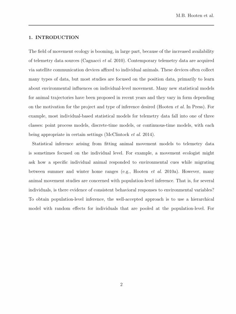
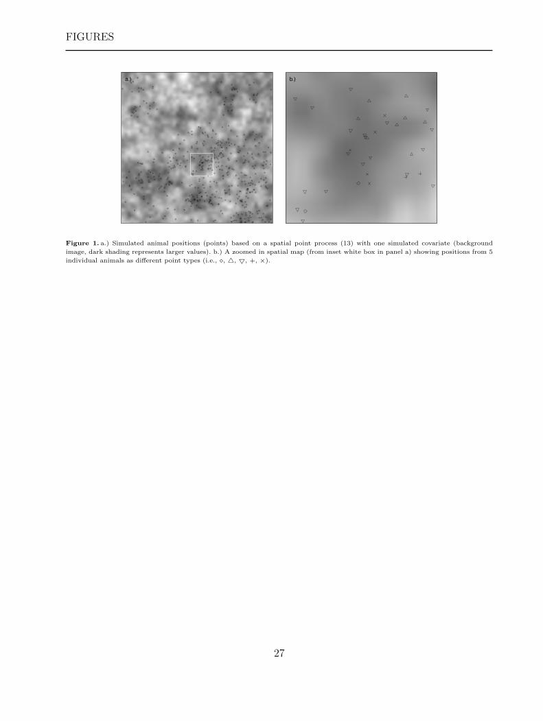
We simulated point process data from 20 individuals (Figure 1), resulting in approximately

30 simulated telemetry fixes per individual, and fit the hierarchical RSF model using: 1.) a

single MCMC algorithm, and 2.) our two-stage procedure. We compared the population-level

results from the fits resulting from each procedure.

11

M.B. Hooten et al.

[Figure 1 about here.]

For the first-stage algorithm in our two-stage procedure, we fit the individual-level models

independently using an adaptive MCMC algorithm in parallel using R (R Core Team 2016)

and assumed N(0, 100 · I) priors for βj, a N(0, 100 · I) prior for µβ, and a Wish((3 · I)−1, 3)

prior for Σ−1β . Our first-stage algorithm uses a multivariate Gaussian proposal for βj and

adapts the tuning using a single variance parameter, resulting in an unsupervised algorithm

for the individual-level model fits. We could have also used BUGS or JAGS to fit the first-

stage models, but our adaptive MCMC algorithm required less computing time.

The single MCMC algorithm to fit the full hierarchical model required 2.62 minutes to

obtain 20,000 MCMC samples in R, whereas the first-stage algorithm required 0.57 minutes

to obtain the same number of samples using an adaptive MCMC algorithm in parallel for the

20 individuals. The second-stage algorithm required only 1.49 minutes in R, which implies

that the total compute time to fit the model using the two-stage procedure was 2.06 minutes

(0.56 minutes less than the single MCMC algorithm). Also, the two-stage procedure requires

no tuning and results in much larger effective MCMC sample sizes for parameters. The

effective MCMC sample sizes for µβ and βj were 8560 and 1398 (averaged across individuals)

for the single MCMC algorithm, but were 17590 and 15184 for the two-stage algorithm (out

of 20,000 total samples). Thus, to obtain the same effective MCMC sample size using MCMC

for all parameters, we would need an order of magnitude more samples from the single MCMC

algorithm.

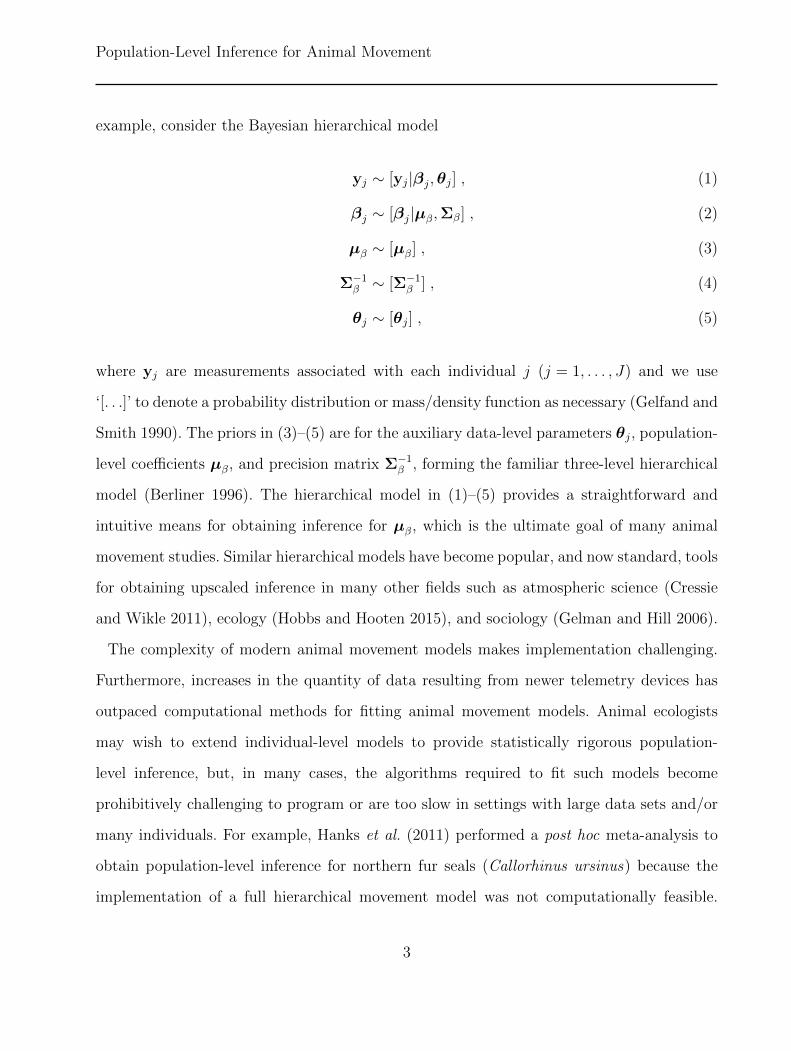
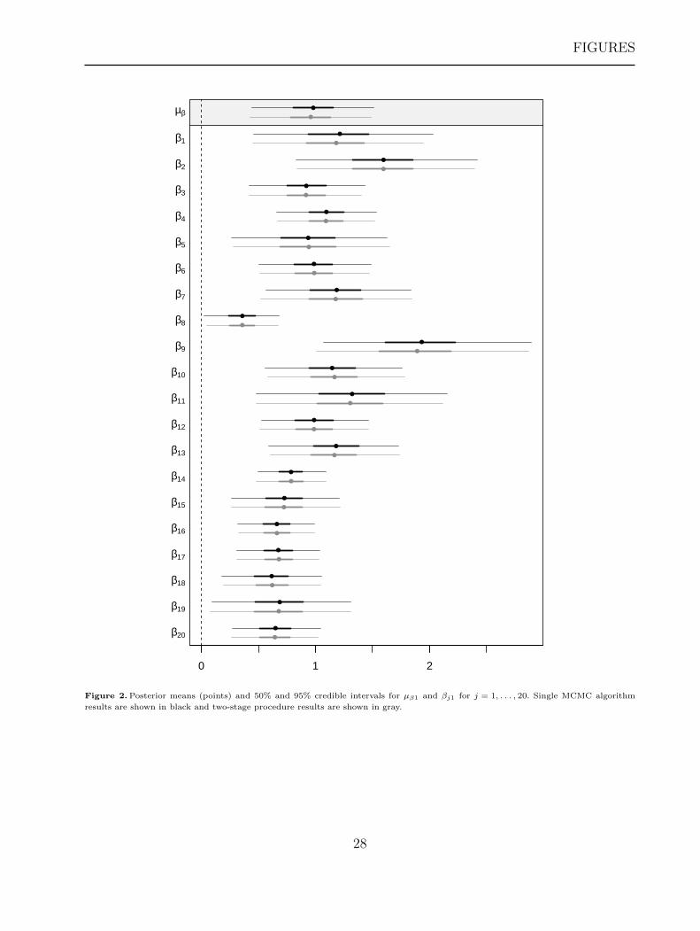
Figure 2 illustrates the similarities in inference for the slope parameters µβ1 and βj1 for

j = 1, . . . , 20 when fitting the hierarchical RSF model using a single MCMC algorithm (black)

versus the two-stage procedure (gray).


Notice that the single MCMC algorithm and the two-stage procedure provide very similar

inference. In terms of inference, there exists some variability among individuals, but the

12


population-level inference (Figure 2, top) suggests a consistent overall positive population

response to the covariate.

3.2. Hierarchical Continuous-Time Discrete-Space Models

The previous application, involving spatial point process models, involves a commonly

used model specification and desired type of inference in ecological research, but more

contemporary methods have been developed to explicitly model the dynamics of animal

movement based on temporally dependent telemetry data with observations close in time.

Among these methods are discrete-time and continuous-time approaches to modeling the

individual animal trajectories (McClintock et al. 2014). We focus on the continuous-time

class of models in what follows.

Continuous-time statistical models for animal movement processes have existed for decades

(e.g., Dunn and Gipson 1977; Blackwell 1997), and are usually based on Brownian motion

(i.e., Wiener processes). Up until the late 1990s, most Brownian motion models for

trajectories utilized an Ornstein-Uhlenbeck process (i.e., a Wiener process with attraction to

a central position). Johnson et al. 2008b also proposed an Ornstein-Uhlenbeck model, but for

the velocity (i.e., temporally differentiated position) rather than the position process. Hooten

and Johnson (2016a) generalized the continuous-time velocity models of Johnson et al.

(2008b) in the context of Gaussian processes with covariance structure induced by temporal

basis functions. Buderman et al. (2016) used a simplified basis function parameterization to

model Canada lynx (Lynx canadensis) movement while accounting for measurement error in

the telemetry data. Buderman et al. (2016) refer to their model as a “functional movement

model” and use it to provide inference for the true underlying continuous position process

(i.e., µ(t), for time t) of an individual.

The approach developed by Buderman et al. (2016) assumes that the telemetry data sij

are observed with error. In fact, for the Canada lynx in our study, the bivariate measurement

13

M.B. Hooten et al.

error follows an unusual X-shaped pattern because the telemetry data are collected by Service

Argos (Costa et al. 2010) which relies on polar orbiting satellites. Thus, Brost et al. (2015)

and Buderman et al. (2016) developed a measurement error model based on a mixture

distribution to account for the X-shaped Argos pattern (see Appendix A for details). Properly

accounting for measurement error adds another level to the hierarchical model in (1)–(5) such

that

sij ∼ [sij|µj(ti),φj] , (21)

yj ∼ [yj|βj,θj] , (22)

βj ∼ [βj|µβ,Σβ] , (23)

µβ ∼ [µβ] , (24)

Σ−1β ∼ [Σ−1

β ] , (25)

θj ∼ [θj] , (26)

φj ∼ [φj] , (27)

for j = 1, . . . , J individuals, and where yj is an mj × 1 vector that represents a latent process

that is linked to the true continuous position process {µj(t),∀t} by a deterministic functional

h such that yj = h({µj(t),∀t}), and φj are measurement error covariance parameters.

Hooten et al. (2010a) developed an individual-level animal movement model based on

(21) and (22) where the latent variables yj represent a sequential multinomial process

indicating transitions among grid cells on a discretization of the spatial support S. The latent

process model in (22) relies on a continuous-time discrete-space (CTDS) representation of the

position process. However, because the functional h(·), that links the position process with

the data, is non-invertible in their model, Hooten et al. (2010a) proposed a Bayesian multiple

imputation procedure to account for uncertainty in the true position process when making

inference on βj. The multiple imputation procedure used by Hooten et al. (2010a) differs

14


from the two-stage procedure we described herein because it does not allow for feedback from

the individual-level parameters βj to the position process {µj(t),∀t} or measurement error

parameters φj. Hooten et al. (2010a) used an imputation model to interpolate the position

process and then integrated over the uncertainty in the position process while fitting (22) to

provide posterior inference for the individual-level parameters βj.

Hanks et al. (2015a) showed that the multinomial process of Hooten et al. (2010a) could be

reparameterized such that [yj|βj,θj] can be modeled using Poisson regression. Specifically,

let τcj represent the amount of time individual j remains in a grid cell for the cth “stay/move”

pair associated with the discretization of the individual’s path through a landscape (for

c = 1, . . . , nj). Then let yclj ∼ Pois(τcj exp(x′cljβj)) where the index l = 1, 2, 4, 5 (l = 3 is

not necessary because corresponds to the middle cell which is captured by τcj) denotes

moves to neighboring grid cells in each cardinal direction (i.e., north, east, south, west).

That is, if individual j moved north for “stay/move” pair c, then the data point yc1j = 1

and yc2j = yc3j = yc4j = 0 (see Appendix B for details). The Poisson reparametrization

dramatically improves computational efficiency at the individual level because the total

number of observations used in the model (4mj) is a function of the grid cell size rather

than the position process discretization as used in Hooten et al. (2010a). Thus, Hanks et al.

(2015a) were able to fit the CTDS model to large telemetry data sets in a fraction of the time

required by the multinomial method developed by Hooten et al. (2010a). However, neither

Hooten et al. (2010a) nor Hanks et al. (2015a) attempted to fit a hierarchical model like that

in (21)—(27) to obtain population level inference for µβ.

In our application involving population-level inference for Canada lynx, we use the model

developed by Buderman et al. (2016) to obtain the imputation distribution for the true

individual-level position process {µj(t),∀t}, and hence yclj for all c, l, and j, while accounting

for the complicated nature of Argos telemetry error (see Appendix A for details). In what

follows, we combine all yclj into a single vector representing the latent process yj and use yj

15

M.B. Hooten et al.

as data in a two-stage implementation of the hierarchical model in (21)–(27).

To fit the hierarchical model using the two-stage procedure described in Section 2, we

apply the same two stages of algorithms as in the previous application. For the first stage,

we use the data model in (22) and specify multivariate Gaussian priors for the individual-

level parameters βj ∼ N(µ0,Σ0). We use an adaptively-tuned MCMC algorithm to obtain

samples from the posterior distributions

[βj|{sij,∀i, j}] =

∫[βj|yj][yj|{sij, ∀i, j}]dyj , (28)

for j = 1, . . . , J , and where, [yj|{sij,∀i, j}] represents the imputation distribution for

the latent Poisson process. To perform the integration in (28), we simply sample ykj ∼

[yj|{sij,∀i, j}] on the kth MCMC iteration and then let the Metropolis-Hastings update

βkj depend on ykj as described in Hooten et al. (2010a) and Hanks et al. (2015a). As in the

first application, we can fit the J models for all individuals in parallel, dramatically reducing

the required computational time.

For the second stage of the two-stage procedure, we use the posterior samples for {βj,∀j},

from the first stage, as proposals in the MCMC algorithm to fit the hierarchical model in (22)–

(25). In doing so, we update {βj,∀j}, µβ, and Σ−1β sequentially in a completely unsupervised

second-stage MCMC algorithm. Recall that the Metropolis-Hastings acceptance ratio for

βj is identical to that used in the previous application (20). As a result of the two-

stage implementation and the adaptive tuning in the first-stage algorithm, the procedure is

completely automatic after the data are preprocessed to obtain the imputation distribution,

and population-level inference for µβ can easily be obtained.

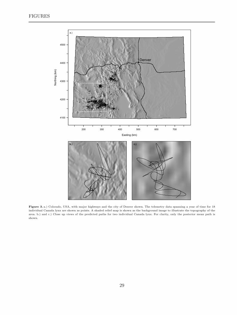
Using telemetry data from J = 18 individual Canada lynx in Colorado, USA (Figure 3a),

we applied the two-stage procedure to fit the hierarchical model in (22)–(25).


16


We used the functional movement model of Buderman et al. (2016) to obtain the imputed

path distribution (Figure 3b,c) for each individual and used nearly continuous imputed path

realizations to create the latent Poisson data realizations ykj (resulting in approximately 450

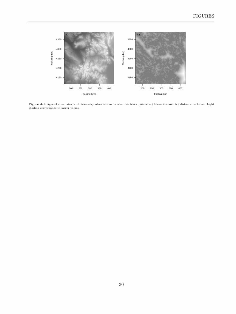
discrete-space transitions per individual, nj ≈ 450). Canada lynx are a subalpine species that

tend to prefer forested ecosystems (McKelvey et al. 2000), thus we focused on two covariates:

elevation and distance to forest (Figure 4).


Each covariate was included in the model as a “static” driver, rather than a gradient-based

driver of movement (Hanks et al. 2015a). Static drivers can be interpreted as affecting overall

motility in the CTDS model. For priors in the first stage, we used βj ∼ N(0, 100I) for

all j = 1, . . . , 18. We used µβ ∼ N(0, 100I) and Σ−1β ∼Wish((3 · I)−1, 3) as priors for the

population-level parameters and precision matrix. See Appendix B for additional details on

the CTDS animal movement model.

We fit the overall hierarchical model using the two-stage procedure and the resulting

algorithms required 0.86 minutes for the first stage (using an adaptive MCMC algorithm

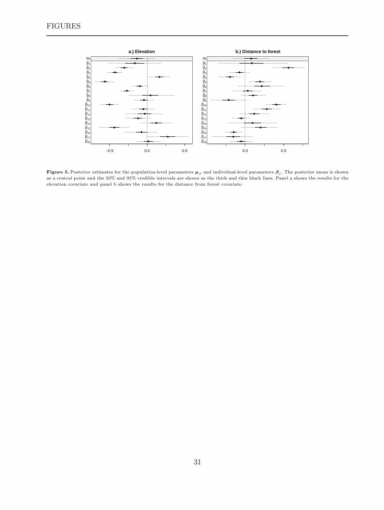
in parallel) and 1.62 minutes for the second stage. Figure 5 shows the results of the model

fit in terms of posterior means and 50% and 95% credible intervals for the population-level

parameters µβ and individual-level parameters βj.


While there exists substantial variability among individual Canada lynx, with some

individuals exhibiting clear relationships with the covariates (e.g., individuals 2, 4, and 5), the

posterior distributions for µ did not indicate a population-level effect for either covariate at

the 95% level (but both did at the 50% level). For the individuals that did show evidence of an

effect (i.e., 95% credible intervals not overlapping zero), the negative response to elevation

indicates that overall motility decreases at higher elevations, leading to greater residence

times in those regions, as opposed to lower elevations (Figure 5a). Similarly, for individuals

17

M.B. Hooten et al.

with significant effects related to distance from forest we see positive influence on motility

implying that those Canada lynx have higher motility (and hence lower residence time)

in regions farther from forest (Figure 5b). Thus, the inference in our application involving

Canada lynx agrees with that obtained in other studies (e.g., McKelvey et al. 2000).

4. CONCLUSION

Our findings indicate that the two-stage procedure we described herein holds tremendous

value for fitting hierarchical animal movement models to telemetry data for population-

level inference. We applied the two-stage procedure to two types of commonly used animal

movement models of varying complexity and found that it worked well in both cases.

The spatial point process modeling approach we described in the first application is a

commonly used model, but still fairly simple. Much more complicated spatio-temporal point

process models have been used to model temporally correlated telemetry data (e.g., Johnson

et al. 2008a; Johnson et al. 2013; Brost et al. 2015) and adapting the two-stage procedure to

those models is the subject of ongoing research. For example, Brost et al. (2015) developed a

model with a time-varying dynamic availability component that depended on an additional

smoothness parameter. Thus, the data model developed by Brost et al. (2015) required

substantially more computation time than the simulated example we presented in Section

3.1 and would benefit from a two-stage implementation where individual-level models could

be fit independently on separate processors and then recombined using the second stage

MCMC algorithm to yield population-level inference for µβ.

In our example involving Canada lynx, the continuous-time discrete-space reparameter-

ization developed by Hanks et al. (2015a) already provides significant improvements in

computational efficiency over the motivating model developed by Hooten et al. (2010a).

However, additional computational gains can be achieved using the two-stage fitting

18


procedure to provide population-level inference.

Despite the wide range of potential applications to many types of hierarchical models,

we found it surprising that the two-stage fitting procedure of Lunn et al. (2013) is not

more well known. For our situations with large amounts of telemetry data and potentially

complicated data models, we found the two-stage procedure works very well and is trivial to

implement. We also found it very helpful to be able to use different data models, first-stage

fitting algorithms, and easy parallelization. As a potential caveat, the two-stage procedure

described by Lunn et al. (2013) may not be very efficient when the population induces

extreme amounts of shrinkage in the individual-level parameters. Thus, in these cases, more

samples would be needed in the first stage algorithm. However, in a preliminary simulation

study, we found that the two-stage procedure performs poorly only for data sets with very

small amounts of data (i.e., < 20 observations for a subset of individuals).

Animal movement models have also been developed to account for more mechanistic

interactions among individuals (e.g., Russell et al. 2016; Scharf et al. 2015) and, while we

did not address those specifically, the approach we presented may also be beneficial in those

settings. Furthermore, Bayesian animal movement models have been fit using integrated

nested Laplace approximation (INLA; Rue et al. 2009; Illian et al. 2012; Illian et al. 2013;

Ruiz-Cardenas et al. 2012; Jonsen 2016) and one could use INLA to fit the hierarchical point

process model in our first example. However, the two-stage MCMC approach presented herein

allows for: Inference on joint relationships among model parameters, easy parallelization in

the first stage, and the ability to use Bayesian multiple imputation techniques, such as in

our second example involving the CTDS movement model.

19

M.B. Hooten et al.

ACKNOWLEDGEMENTS

Support for this research was provided by NSF 1614392, NSF EEID 1414296, CPW T01304,

and NOAA AKC188000. The authors thank The International Environmetrics Society and

the editors of Environmetrics for their support and assistance with this work. The authors

also thank Walt Piegorsch, Mindy Rice, Devin Johnson, Peter Craigmile, Erin Peterson, Ron

Smith, and the other organizers of the TIES 2016 annual meeting. Any use of trade, firm,

or product names is for descriptive purposes only and does not imply endorsement by the

U.S. Government.

REFERENCES

Aarts G, Fieberg J, Matthiopoulos J, 2012. Comparative interpretation of count, presence-absence, and point

methods for species distribution models. Methods in Ecology and Evolution 3: 177–187.

Berliner L, 1996. Hierarchical Bayesian time series models. In Hanson K, Silver R (eds.), Maximum Entropy

and Bayesian Methods, Kluwer Academic Publishers, 15–22.

Blackwell P, 1997. Random diffusion models for animal movement. Ecological Modelling 100: 87–102.

Bradley J, Holan S, Wikle C, 2015. Computationally efficient distribution theory for Bayesian inference of

high-dimensional dependent count-valued data. arXiv preprint arXiv:1512.07273 .

Brost B, Hooten M, Hanks E, Small R, 2015. Animal movement constraints improve resource selection

inference in the presence of telemetry error. Ecology 96: 2590–2597.

Buderman F, Hooten M, Ivan J, Shenk T, 2016. A functional model for characterizing long distance movement

behavior. Methods in Ecology and Evolution 7: 264–273.

Cagnacci F, Boitani L, Powell RA, Boyce MS, 2010. Animal ecology meets gps-based radiotelemetry: a

perfect storm of opportunities and challenges. Philosophical Transactions of the Royal Society of London

B: Biological Sciences 365: 2157–2162.

Carpenter B, Gelman A, Hoffman M, Lee D, Goodrich B, Betancourt M, Brubaker M, Guo J, Li P, Riddell

A, 2016. Stan: a probabilistic programming language. Journal of Statistical Software .

Costa D, Robinson P, Arnould J, Harrison AL, Simmons SE, Hassrick JL, Hoskins AJ, Kirkman SP,

Oosthuizen H, Villegas-Amtmann S, Crocker DE, 2010. Accuracy of Argos locations of pinnipeds at-sea

20


estimated using Fastloc GPS. PLoS One 5: e8677.

Cressie N, Wikle C, 2011. Statistics for Spatio-Temporal Data. John Wiley and Sons, New York, New York,

USA.

Crooks G, 2010. The amoroso distribution. arXiv preprint arXiv:1005.3274 .

Dunn J, Gipson P, 1977. Analysis of radio-telemetry data in studies of home range. Biometrics 33: 85–101.

Gamerman D, 1997. Sampling from the posterior distribution in generalized linear mixed models. Statistics

and Computing 7: 57–68.

Gelfand A, Smith A, 1990. Sampling-based approaches to calculating marginal densities. Journal of the

American Statistical Association 85: 398–409.

Gelman A, Hill J, 2006. Data Analysis Using Regression and Multilevel/Hierarchical Models. Cambridge

University Press, Cambridge, United Kingdom.

Givens G, Hoeting J, 2012. Computational Statistics, volume 710. John Wiley & Sons.

Hanks E, Hooten M, Alldredge M, 2015a. Continuous-time discrete-space models for animal movement.

Annals of Applied Statistics 9: 145–165.

Hanks E, Hooten M, Johnson D, Sterling J, 2011. Velocity-based movement modeling for individual and

population level inference. PLoS One 6: e22795.

Hobbs N, Hooten M, 2015. Bayesian Models: A Statistical Primer for Ecologists. Princeton University Press,

Princeton, New Jersey, USA.

Hooten M, Johnson D, 2016a. Basis function models for nonstationary continuous-time trajectories. Journal

of the American Statistical Association : In Revision.

Hooten M, Johnson D, Hanks E, Lowry J, 2010a. Agent-based inference for animal movement and selection.

Journal of Agricultural, Biological and Environmental Statistics 15: 523–538.

Hooten M, Johnson D, McClintock B, Morales J, In Press. Animal Movement: Statistical Models for

Telemetry Data. Chapman & Hall/CRC.

Illian J, Martino S, Sørbye S, Gallego-Fernandez J, Zunzunegui M, Esquivias M, Travis J, 2013. Fitting

complex ecological point process models with integrated nested Laplace approximation. Methods in Ecology

and Evolution 4: 305–315.

Illian J, Sorbye S, Rue H, Hendrichsen D, 2012. Using INLA to fit a complex point process model with

temporally varying effects - a case study. Journal of Environmental Statistics 3: 1–25.

21

M.B. Hooten et al.

Johnson D, Hooten M, Kuhn C, 2013. Estimating animal resource selection from telemetry data using point

process models. Journal of Animal Ecology 82: 1155–1164.

Johnson D, London J, Lea M, Durban J, 2008b. Continuous-time correlated random walk model for animal

telemetry data. Ecology 89: 1208–1215.

Johnson D, Thomas D, Ver Hoef J, Christ A, 2008a. A general framework for the analysis of animal resource

selection from telemetry data. Biometrics 64: 968–976.

Jonsen I, 2016. Joint estimation over multiple individuals improves behavioural state inference from animal

movement data. Scientific Reports 6: 20625.

Jonsen I, Flemming J, Myers R, 2005. Robust state-space modeling of animal movement data. Ecology 45:

589–598.

Lunn D, Barrett J, Sweeting M, Thompson S, 2013. Fully Bayesian hierarchical modelling in two stages,

with application to meta-analysis. Journal of the Royal Statistical Society: Series C (Applied Statistics)

62: 551–572.

Lunn D, Spiegelhalter D, Thomas A, Best N, 2009. The BUGS project: Evolution, critique and future

directions. Statistics in Medicine 28: 3049–3067.

Manly B, McDonald L, Thomas D, McDonald T, Erickson W, 2007. Resource Selection by Animals: Statistical

Design and Analysis for Field Studies. Springer Science & Business Media.

McClintock B, Johnson D, Hooten M, Ver Hoef J, Morales J, 2014. When to be discrete: the importance of

time formulation in understanding animal movement. Movement Ecology 2: 21.

McKelvey K, Aubry K, Ortega Y, 2000. History and distribution of lynx in the contiguous United States.

In Ruggiero L, Squires J, Buskirk S, Aubry K, McKelvey K, Koehler G, Krebs C (eds.), Ecology and

Conservation of Lynx in the United States, University Press of Colorado, Boulder, Colorado, USA, 207–

264.

Murray L, 2013. Bayesian state-space modelling on high-performance hardware using libBi. arXiv preprint

arXiv:1306.3277 .

Patil G, Rao C, 1977. The weighted distributions: a survey of their applications. In Krishnaiah P (ed.),

Applications of Statistics, North Holland Publishing Company.

Plummer M, 2003. JAGS: A program for analysis of Bayesian graphical models using Gibbs sampling. In

Proceedings of the 3rd international workshop on distributed statistical computing, volume 124, Technische

Universit at Wien Wien, Austria, 125.

22


R Core Team, 2016. R: A Language and Environment for Statistical Computing. R Foundation for Statistical

Computing, Vienna, Austria.

Roberts G, Rosenthal J, 2009. Examples of adaptive MCMC. Journal of Computational and Graphical

Statistics 18: 349–367.

Rue H, Martino S, Chopin N, 2009. Approximate Bayesian inference for latent Gaussian models by using

integrated nested Laplace approximations. Journal of the Royal Statistical Society: Series B (Statistical

Methodology) 71(2): 319–392.

Ruiz-Cardenas R, Krainski E, Rue H, 2012. Direct fitting of dynamic models using integrated nested Laplace

approximations INLA. Computational Statistics & Data Analysis 56: 1808–1828.

Russell JC, Hanks EM, Haran M, Hughes DP, 2016. A spatially-varying stochastic differential equation

model for animal movement. arXiv preprint arXiv:1603.07630 .

Scharf H, Hooten M, Fosdick B, Johnson D, London J, Durban J, 2015. Dynamic social networks based on

movement. arXiv : 1512.07607.

Warton D, Shepherd L, 2010. Poisson point process models solve the “pseudo-absence problem” for presence-

only data in ecology. Annals of Applied Statistics 4: 1383–1402.

APPENDIX

APPENDIX A: THE IMPUTATION DISTRIBUTION

Buderman et al. (2016) developed a phenomenological statistical model for estimating

an individual’s underlying continuous-time path based on Argos telemetry data and a

semiparametric regression using temporal basis functions. We used this model to precalculate

an imputation distribution for the true path. For the jth individual, the FMM developed by

23

M.B. Hooten et al.

Buderman et al. (2016) is

sij ∼

N(µj(ti),Σi) with prob. p

N(µj(ti),HΣiH′) with prob. 1− p

, (A.1)

µj(ti) = Wj(ti)α , (A.2)

α ∼ N(0,Σα) , (A.3)

where, sij represent the ith telemetry observation, µj(ti) is the true individual position at

time ti, Σi is an error covariance matrix on the first axis, and HΣiH′ is the error covariance

matrix on a rotated axis (H is a rotation matrix). The probability p allows the telemetry data

to arise from a bivariate Gaussian mixture that captures the X-shaped error pattern inherent

to Argos data. The matrix Wj(ti) contains basis vectors (i.e., b-spline basis vectors) at time

ti for individual j, and α is a set of regression coefficients corresponding to the temporal basis

functions. Buderman et al. (2016) set Σα ≡ Diag(σ2α) and tuned σ2

α to induce regularization

in the model and improve predictive ability (i.e., ridge regression).

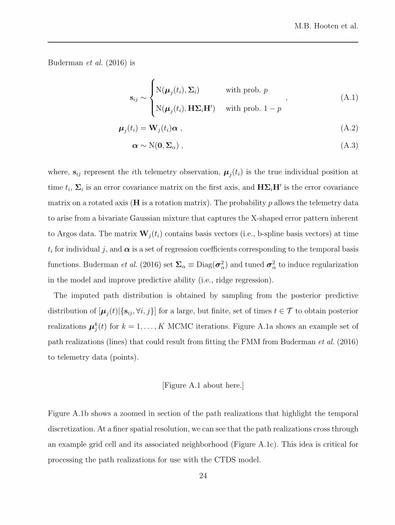
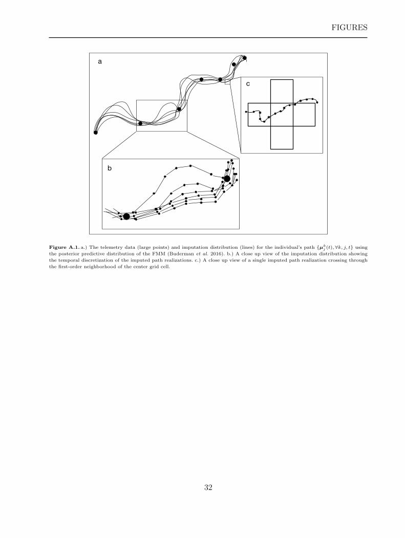
The imputed path distribution is obtained by sampling from the posterior predictive

distribution of [µj(t)|{sij,∀i, j}] for a large, but finite, set of times t ∈ T to obtain posterior

realizations µkj (t) for k = 1, . . . , K MCMC iterations. Figure A.1a shows an example set of

path realizations (lines) that could result from fitting the FMM from Buderman et al. (2016)

to telemetry data (points).

[Figure A.1 about here.]

Figure A.1b shows a zoomed in section of the path realizations that highlight the temporal

discretization. At a finer spatial resolution, we can see that the path realizations cross through

an example grid cell and its associated neighborhood (Figure A.1c). This idea is critical for

processing the path realizations for use with the CTDS model.

24


APPENDIX B: CTDS MODEL

For each individual j in the original CTDS model, each segment (between points) in

Figure A.1c served as a multinomial data vector yij ≡ (y1i, y2i, y3i, y4i, y5i)′j where yij ∼

MN(1,pij) (Hooten et al. 2010a). The multinomial vectors were constructed using the

function yij = h({µj(t),∀t}) based on the imputed path realizations by coding a transition

as either a stay or a move in a certain direction according to the schematic in Figure A.2.

[Figure A.2 about here.]

Hanks et al. (2015a) reparameterized the multinomial imputation data using sufficient

statistics. They denoted residence time as τlj (approximated by ∆t times the number

of consecutive stays in the current grid cell, Figure A.1c) for l = 1, . . . , L “stay–move”

pairs and then defined the probability of staying in the current grid cell for time τlj as

pτlj/∆t3ij = (1− plj,move)

τlj/∆t, where plj,move is the probability of moving. Hanks et al. (2015a)

let plj,move = ∆t · λlj,move and ∆t→ 0 yielding

lim∆t→0

(1− pj,move)τlj/∆t = e−τljλlj,move , (A.4)

which, implies that τlj ∼ Exp(λlj,move).

Similarly, Hanks et al. (2015a) showed that the movement probability to neighboring grid

cell c is pclj/plj,move = λclj/λlj,move. Thus, combing the residence probability model with the

movement probability yields a likelihood for the sufficient statistic (τlj, y1lj, y2lj, y4lj, y5lj)′

equal to∏L

l=1

∏c6=3 λclj exp(−τljλclj). The likelihood for this reparameterized CTDS model

coincides with a Poisson where λclj is the movement rate to neighboring cell c and τlj is an

offset. Thus, any software capable of fitting a Poisson generalized linear model with an offset

can fit the CTDS model if the true path is observed at a fine enough temporal resolution.

Hanks et al. (2015a) used a multiple imputation approach to account for the uncertainty

in the path distribution based on (28). The movement rates can then be linked to the

25

M.B. Hooten et al.

environmental covariates by a log-linear link λclj = x′cljβj, where the covariates x′clj can

be specified in several meaningful ways to capture either differential movement rates (i.e.,

motility) or gradient-based directional bias in movement relative to environmental covariates

(see Hanks et al. 2015a for details). The reparameterized CTDS model of Hanks et al.

(2015a) is much more computationally efficient than that of Hooten et al. (2010a) because

the dimensionality of the data 4L depends on the grid cell size instead of the temporal

discretization of the path.

26

FIGURES

a.)

y

b.)

Figure 1. a.) Simulated animal positions (points) based on a spatial point process (13) with one simulated covariate (background

image, dark shading represents larger values). b.) A zoomed in spatial map (from inset white box in panel a) showing positions from 5

individual animals as different point types (i.e., �, 4, 5, +, ×).

27

FIGURES

●

●

●

●

●

●

●

●

●

●

●

●

●

●

●

●

●

●

●

●

●

●

●

●

●

●

●

●

●

●

●

●

●

●

●

●

●

●

●

●

●

●

0 1 2

β1

β2

β3

β4

β5

β6

β7

β8

β9

β10

β11

β12

β13

β14

β15

β16

β17

β18

β19

β20

µβ

Figure 2. Posterior means (points) and 50% and 95% credible intervals for µβ1 and βj1 for j = 1, . . . , 20. Single MCMC algorithm

results are shown in black and two-stage procedure results are shown in gray.

28

FIGURES

Denver

200 300 400 500 600 700

4100

4200

4300

4400

4500

Nor

thin

g (k

m)

Easting (km)

a.)

b.)b.)

c.)c.)

b.)b.) c.)c.)

Figure 3. a.) Colorado, USA, with major highways and the city of Denver shown. The telemetry data spanning a year of time for 18

individual Canada lynx are shown as points. A shaded relief map is shown as the background image to illustrate the topography of the

area. b.) and c.) Close up views of the predicted paths for two individual Canada lynx. For clarity, only the posterior mean path is

shown.

29

FIGURES

200 250 300 350 400

4150

4200

4250

4300

4350

Nor

thin

g (k

m)

Easting (km)

a.)

200 250 300 350 400

4150

4200

4250

4300

4350

Nor

thin

g (k

m)

Easting (km)

b.)

Figure 4. Images of covariates with telemetry observations overlaid as black points: a.) Elevation and b.) distance to forest. Light

shading corresponds to larger values.

30

FIGURES

a.) Elevation●

●

●

●

●

●

●

●

●

●

●

●

●

●

●

●

●

●

●

−0.5 0.0 0.5

β1

β2

β3

β4

β5

β6

β7

β8

β9

β10

β11

β12

β13

β14

β15

β16

β17

β18

µβ

b.) Distance to forest●

●

●

●

●

●

●

●

●

●

●

●

●

●

●

●

●

●

●

0.0 0.5

β1

β2

β3

β4

β5

β6

β7

β8

β9

β10

β11

β12

β13

β14

β15

β16

β17

β18

µβ

Figure 5. Posterior estimates for the population-level parameters µβ and individual-level parameters βj . The posterior mean is shown

as a central point and the 50% and 95% credible intervals are shown as the thick and thin black lines. Panel a shows the results for the

elevation covariate and panel b shows the results for the distance from forest covariate.

31

FIGURES

a

b

c

Figure A.1. a.) The telemetry data (large points) and imputation distribution (lines) for the individual’s path {µkj (t), ∀k, j, t} using

the posterior predictive distribution of the FMM (Buderman et al. 2016). b.) A close up view of the imputation distribution showing

the temporal discretization of the imputed path realizations. c.) A close up view of a single imputed path realization crossing through

the first-order neighborhood of the center grid cell.

32

FIGURES

a b c d e

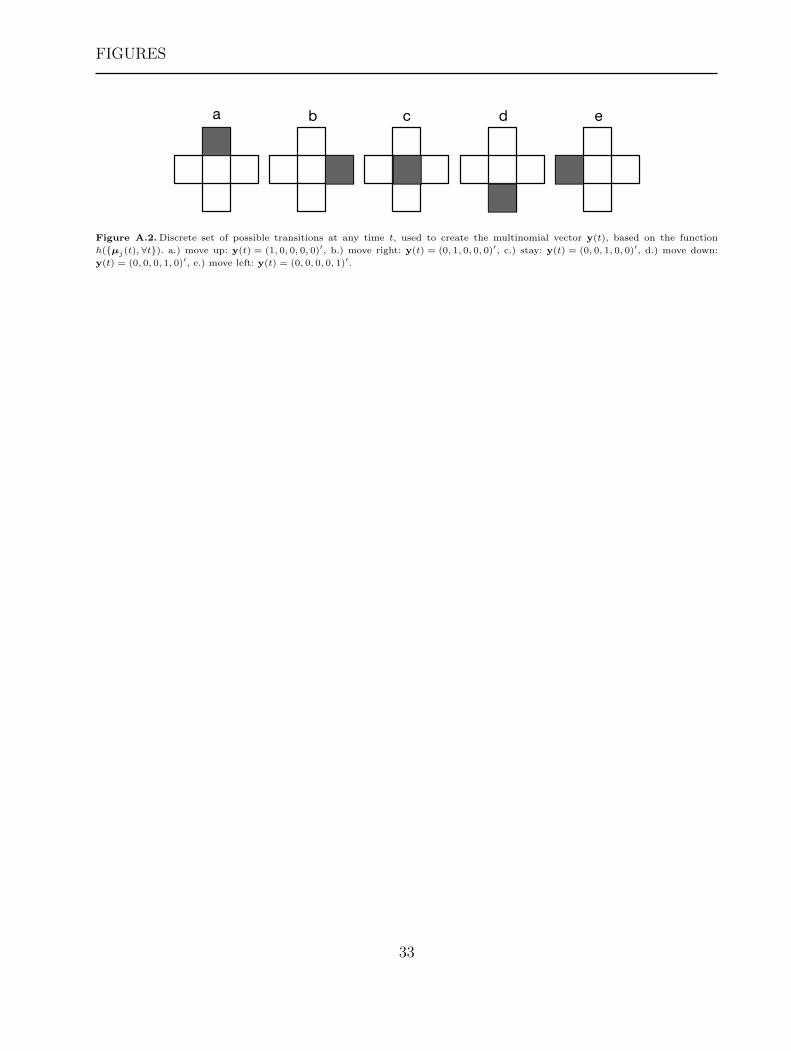
Figure A.2. Discrete set of possible transitions at any time t, used to create the multinomial vector y(t), based on the function

h({µj(t), ∀t}). a.) move up: y(t) = (1, 0, 0, 0, 0)′, b.) move right: y(t) = (0, 1, 0, 0, 0)′, c.) stay: y(t) = (0, 0, 1, 0, 0)′, d.) move down:

y(t) = (0, 0, 0, 1, 0)′, e.) move left: y(t) = (0, 0, 0, 0, 1)′.

33

Hierarchical Animal Movement Models for Population-Level … · Population-Level Inference for...

Documents

Transcript of Hierarchical Animal Movement Models for Population-Level … · Population-Level Inference for...