Hexagon-BasedGeneralizedVoronoiDiagramsGenerationfor ...
13
Research Article Hexagon-Based Generalized Voronoi Diagrams Generation for Path Planning of Intelligent Agents Fen Tang , Xiong You , Xin Zhang , and Kunwei Li College of Geospatial Information, Information Engineering University, Henan, Zhengzhou 450052, China Correspondence should be addressed to Xiong You; [email protected] Received 27 August 2019; Accepted 22 February 2020; Published 23 April 2020 Academic Editor: Ivan Giorgio Copyright © 2020 Fen Tang et al. is is an open access article distributed under the Creative Commons Attribution License, which permits unrestricted use, distribution, and reproduction in any medium, provided the original work is properly cited. Grid-based Generalized Voronoi Diagrams (GVDs) are widely used to represent the surrounding environment of intelligent agents in the fields of robotics, computer games, and military simulations, which improve the efficiency of path planning of intelligent agents. Current studies mainly focus on square-grid-based GVD construction approaches, and little attention has been paid to constructing GVDs from hexagonal grids. In this paper, an algorithm named hexagon-based crystal growth (HCG) is presented to extract GVDs from hexagonal grids. In addition, two thinning patterns for obtaining one-cell-wide GVDs from rough hexagon-based GVDs are proposed. On the basis of the principles of a leading square-grid-based algorithm named Brushfire, a hexagon-based Brushfire algorithm is realized. A comparison of the HCG and the hexagon-based Brushfire algorithm shows that HCG is much more efficient. Further, the usefulness of hexagon-based GVDs for the path planning tasks of intelligent agents is demonstrated using several representative simulation experiments. 1.Introduction Spatial representation is considered to be a fundamental subject in the fields of robotics, computer games, and military simulation. In applications in these fields, one or more intelligent agents frequently implement spatial rea- soning tasks such as route planning, self-localisation, and collision avoidance. Generally speaking, the representation method of the underlying working space significantly in- fluences the efficiency of spatial reasoning algorithms of the intelligent agents. erefore, a sparse and well-structured spatial representation is needed for these agents. ere are many ways to represent the spatial environ- ment, such as regular and irregular grids [1], waypoint graphs [2], probabilistic roadmaps [3], and GVDs [4]. GVDs can represent the sparse skeleton of the entire spatial en- vironment, which reduces the search space and improves the efficiency of path planning algorithms. In addition, GVDs provide the maximum clearance in regions with obstacle so that robots can avoid them. Because of these advantages, research on efficiently constructing the GVDs has recently drawn significant attention. Triangles, squares, and hexagons are the only regular polygons that can be used to tessellate a continuous two-di- mensional (2D) environment [5]. Among them, square grids are the most commonly used, and several GVDs construction algorithms based on them have been proposed, e.g., the Brushfire algorithm [6] and its improved versions (the dy- namic Brushfire algorithm [7] and the method developed by Lau et al. [8]). However, the Brushfire algorithm provides no efficient mechanism for updating partial areas where local changes occur; it abandons the existing GVDs and builds a new one from scratch, making it unacceptable in a dynamic environment. To solve this problem, Kalra et al. proposed the dynamic Brushfire algorithm [7], and Lau et al. developed a novel method (referred to as the BL algorithm in this paper) [8]. Both algorithms can efficiently update GVDs when the underlying environment changes. An algorithm named dy- namic topology detector (DTD) was proposed by Qin et al. [9]. In addition to generating GVDs, it extracts the connectivity among the edges and vertices of the GVDs and provides an efficient repair mechanism to dealing with local changes. As one of the three 2D regular girds, hexagonal grids have been well studied and widely used in many fields. For Hindawi Mathematical Problems in Engineering Volume 2020, Article ID 5750739, 13 pages https://doi.org/10.1155/2020/5750739
Transcript of Hexagon-BasedGeneralizedVoronoiDiagramsGenerationfor ...

Research ArticleHexagon-Based Generalized Voronoi Diagrams Generation forPath Planning of Intelligent Agents
Fen Tang Xiong You Xin Zhang and Kunwei Li
College of Geospatial Information Information Engineering University Henan Zhengzhou 450052 China
Correspondence should be addressed to Xiong You youarexiong163com
Received 27 August 2019 Accepted 22 February 2020 Published 23 April 2020
Academic Editor Ivan Giorgio
Copyright copy 2020 Fen Tang et al +is is an open access article distributed under the Creative Commons Attribution Licensewhich permits unrestricted use distribution and reproduction in any medium provided the original work is properly cited
Grid-based Generalized Voronoi Diagrams (GVDs) are widely used to represent the surrounding environment of intelligentagents in the fields of robotics computer games and military simulations which improve the efficiency of path planning ofintelligent agents Current studies mainly focus on square-grid-based GVD construction approaches and little attention has beenpaid to constructing GVDs from hexagonal grids In this paper an algorithm named hexagon-based crystal growth (HCG) ispresented to extract GVDs from hexagonal grids In addition two thinning patterns for obtaining one-cell-wide GVDs fromrough hexagon-based GVDs are proposed On the basis of the principles of a leading square-grid-based algorithm namedBrushfire a hexagon-based Brushfire algorithm is realized A comparison of the HCG and the hexagon-based Brushfire algorithmshows that HCG is much more efficient Further the usefulness of hexagon-based GVDs for the path planning tasks of intelligentagents is demonstrated using several representative simulation experiments
1 Introduction
Spatial representation is considered to be a fundamentalsubject in the fields of robotics computer games andmilitary simulation In applications in these fields one ormore intelligent agents frequently implement spatial rea-soning tasks such as route planning self-localisation andcollision avoidance Generally speaking the representationmethod of the underlying working space significantly in-fluences the efficiency of spatial reasoning algorithms of theintelligent agents +erefore a sparse and well-structuredspatial representation is needed for these agents
+ere are many ways to represent the spatial environ-ment such as regular and irregular grids [1] waypointgraphs [2] probabilistic roadmaps [3] and GVDs [4] GVDscan represent the sparse skeleton of the entire spatial en-vironment which reduces the search space and improves theefficiency of path planning algorithms In addition GVDsprovide the maximum clearance in regions with obstacle sothat robots can avoid them Because of these advantagesresearch on efficiently constructing the GVDs has recentlydrawn significant attention
Triangles squares and hexagons are the only regularpolygons that can be used to tessellate a continuous two-di-mensional (2D) environment [5] Among them square gridsare the most commonly used and several GVDs constructionalgorithms based on them have been proposed eg theBrushfire algorithm [6] and its improved versions (the dy-namic Brushfire algorithm [7] and the method developed byLau et al [8]) However the Brushfire algorithm provides noefficient mechanism for updating partial areas where localchanges occur it abandons the existing GVDs and builds anew one from scratch making it unacceptable in a dynamicenvironment To solve this problem Kalra et al proposed thedynamic Brushfire algorithm [7] and Lau et al developed anovel method (referred to as the BL algorithm in this paper)[8] Both algorithms can efficiently update GVDs when theunderlying environment changes An algorithm named dy-namic topology detector (DTD)was proposed byQin et al [9]In addition to generating GVDs it extracts the connectivityamong the edges and vertices of the GVDs and provides anefficient repair mechanism to dealing with local changes
As one of the three 2D regular girds hexagonal gridshave been well studied and widely used in many fields For
HindawiMathematical Problems in EngineeringVolume 2020 Article ID 5750739 13 pageshttpsdoiorg10115520205750739
example the hexagonal grid has long been known to besuperior to the more traditional rectangular grid system inmany aspects in image processing and machine visionfields [10] In [11] a hexagonal image processing frame-work was proposed advantages and disadvantages ofwhich were also explained In [12] a simple formula wasderived for the distance between two points on a hexagonalgrid in terms of coordinates with respect to a pair ofoblique axes In [13] the binary tomography recon-struction problem of images on the hexagonal grid wasstudied and a (near) optimal solution was found In ad-dition to the applications in image processing hexagonalgrids have important applications in other fields Forexample Quijano and Garrido [14] simulated robot ex-ploration algorithms based on hexagonal grids +eyproved that these algorithms outperform those on qua-drangular grids for both single and multiagent problemsChrpa and Komenda [15] proposed a method to smooththe trajectory of a helicopter based on hexagonal grids andextended their method to multiagent pathfinding [16] Anumber of computer games eg Wartile and World ofWarships use hexagonal grids to represent the gameworld In military simulations the Joint +eater LevelSimulation (JTLS) system of the United States also useshexagonal grids to represent the terrain of the battlefieldHexagonal grids have many advantages over square gridsFirst when dividing the same area hexagonal grids pro-vide a higher spatial resolution than square grids [17]Second each cell in a hexagonal grid has six neighbourswhose cell centroids are at the same distance [18] as seenin Figure 1 +ird hexagonal grids suffer less from ori-entation bias and sampling bias from edge effects since thedistances to the centroids of the six adjacent cells are thesame [19]
+e square-grid-based GVDs generated from square-grid-based map can help to improve the efficiency of pathplanning tasks of intelligent agents However methodsthat employ this GVDs construction technique are notused in robotics computer games and military simula-tions where the environments are represented withhexagonal grids To date there are no related studies thathave focused on hexagon-based GVD generation for thepath planning of intelligent agents Pathfinding tasks onhexagonal grids are quantitatively implemented by intel-ligent agents in these fields with the Morris [20] Alowast anditerative deepening Alowast (IDAlowast) [21] algorithms being themost commonly used However their time and spacecomplexities dramatically increase when the search areabecomes larger or the number of hexagonal grids in-creases In order to improve the efficiency of path planningtasks in a hexagon-based environment the ability toconstruct hexagon-based GVDs is crucial for an intelligentagent that moves in a large area
+e main focus of this paper is to construct GVDsfrom a preexisting hexagon-based representation of anenvironment An algorithm named hexagon-based crystalgrowth (HCG) is presented which extracts GVDs from ahexagonal grid map Further two thinning patterns areproposed to obtain one-cell-wide GVDs from rough
hexagon-based GVDs +en HCG is compared to thehexagon-based Brushfire algorithm +e usefulness ofhexagon-based GVDs for the path planning tasks ofagents is also demonstrated with some simulationscenarios
+e outline of this paper is as follows First existingGVD construction algorithms are briefly reviewed Amongthe leading algorithms for extracting GVDs from square gridmaps the Brushfire algorithm is the most fundamentalOwing to geometric differences between square and hex-agonal grids the Brushfire algorithm cannot be directlyapplied to hexagon-based GVD construction and needs to bemodified to accommodate hexagonal grids Next the processof constructing a hexagonal grid occupation map is detailed+en the data structure employed by the presented algo-rithms is presented After that the hexagon-based Brushfirealgorithm HCG and two thinning patterns are presentedall of which are illustrated through pseudocode Next HCGis compared with the hexagon-based Brushfire algorithmand the usefulness of hexagon-based GVD metrics for pathplanning tasks is tested Finally the conclusions arepresented
2 Related Work
Voronoi diagrams named after Georgy Voronoi have beenused to address different problems in various fields in-cluding anthropology archaeology astronomy biologycartography chemistry computational geometry geogra-phy robotics and planning [22] To address the complexityof real-world problems a number of advanced Voronoidiagrams have been developed eg weighted Voronoi di-agrams [23] city Voronoi diagrams [24] and GVDs [4] Inthe field of robotics GVDs have been extensively used toplan a path that stays as far away from obstacles as possibleAs a reduced search space it can help to reduce computationtime significantly
Existing algorithms for building 2D GVDs can beroughly divided into two types according to the type of inputdata vector data and raster data which are called vector- andraster-based algorithms respectively [25] GVDs built byvector-based algorithms are accurately and sparsely repre-sented as a set of parametric lines or curves which separatedifferent sites in space [26 27] +ere are also local updatemechanisms for various local changes eg moving sites [28]and inserted or deleted sites [29] Despite these advantagesvector-based algorithms are not suitable for robots whoseworking spaces are represented as grid maps
Raster-based algorithms are very practical for grid mapsand they have received a significant amount of attention Asdiscussed in the previous section most existing raster-basedalgorithms eg the Brushfire dynamic Brushfire BL andDTD algorithms are based on square-grid maps Althoughthe performance and application scenarios of these algo-rithms are different similarities in their algorithmic prin-ciples exist +ey all need to generate three metric matrices(dists obsts and voros) to represent a GVD +e matrix distsstores the discrete or actual Euclidean distance between anarbitrary entry (denoted by s) and the site cell from which s
2 Mathematical Problems in Engineering
propagates +e matrix obsts registers the site identifier andthe coordinates of the exact site cell to which s is currentlythe closest Finally the matrix voros is a Boolean matrix thatindicates whether s is a GVD cell [9] Figure 2 shows thethree matrices Some other researchers have improved someof these algorithms For example Scherer et al propagatedthe actual Euclidean distance instead of the grid steps usedby the dynamic Brushfire algorithm from the exact sourcecell to greatly reduce the relative error [30] By using theldquothinning patternsrdquo proposed in [31] Lau et al providedadditional thinning steps to obtain one-cell-wide edgeswhich makes the resulting GVD edges sparser
3 Construction of a Hexagonal-GridOccupation Map
Hexagonal grids are used to discretise the maximum activespace of intelligent agents As illustrated in Figure 3 themaximum manoeuvring range of an agent is a rectangulararea the length and width of which are denoted by L and W
respectively +e length of the edge of each hexagon isdenoted by r and the distance from the centre of a hexagonto its edge is denoted by h
+e hexagonal grid is indexed as ldquoColIDndashRowIDrdquo whereldquoColIDrsquo and lsquoRowIDrdquo are the indices of the column and rowin the grid respectively Given the maximum ColID col andmaximum RowID row r can be calculated by
r min2 times L
3 times col + 1
W3
radictimes row
1113888 1113889 (1)
For the cells in the even columns the coordinates of thecentre point of each hexagonal grid can be calculated by
x intColID
21113888 1113889 times 3 + 11113890 1113891 times r
y (2 times RowID + 1) times h
⎧⎪⎪⎪⎪⎨
⎪⎪⎪⎪⎩
(2)
For the cells in the odd columns the coordinates of thecentre point of each hexagonal grid can be calculated by
(a) (b) (c)
Figure 1 Square grids with (a) four and (b) eight neighbours (c) Hexagonal grid with six neighbours
000000000000000000000000
111111111111111111111110
222222222222222222222210
222223333333333333333210
111113333333333444443210
000012322222222344543210
111012211111111344543210
221012210000001234543210
321012210111101124543210
321012210122101234543210
321012210111101234543210
321012210000001234543210
321012211111111234543210
321012322222222344543210
321012333333333445543210
321012344444444456543210
321112344445555566543210
432223333344566676543210
432222222234567776543210
321111111123456776543210
321000000123456776543210
321011110123456776543210
321012210123456776543210
321011110123456776543210
(a)
131
11
111
1111
11111
111111
111111
111111
111111
511111
511111
111111
111111
111111
111111
1111111
1111111
11111111
11111111
11111111
11111111
11111111
11111111
66666
66666666
6666666666666666
6666666666666666
6666666666666666
6666666666666666
6666666666666666
6666666666666666
777777
7
777777
777777
777777
777777
777777
777777
777777
777777
777777
777777
777777
77777777
7
7777777
777777
33333333333333333333333
3333333333333333333333
3333333333333333333333
333333333333333
3333
3
555555555
555555555555
555555555555
555555555555
555555555555
555555555555
555555555555
555555555555
555555555555
555555555555
55555555555
5555555555
55555
555
(b)
000
00
000
0000
00000
100000
100000
100000
100000
100000
100000
100000
100000
000000
000000
0000000
0000000
00000000
00000000
00000000
00000000
00000000
10000000
11100
00001100
1111100000001101
0000000000000011
0000000000000001
0000000000000001
0000011000000001
0000000000000000
100011
1
000000
000000
000000
000001
000000
000001
000000
000001
000001
000000
000000
00000001
1
0000001
000001
00000000000000000000000
0000000000000000000000
0111000000000000000000
000011000000000
1000
0
111001111
010000000001
100000000000
000000000000
100000000000
000011000000
100000000000
000000000000
000000000000
100000000000
00000000001
0000000001
00001
001
(c)
Figure 2 +ree GVD matrices constructed by the Brushfire dynamic Brushfire BL and DTD algorithms (a) corresponding dists matrixwhere each entry stores the integral distance to its nearest site cell (b) corresponding obsts matrix where each entry stores the site identifierand the exact coordinates (not represented here) of its nearest site cell and (c) corresponding vorosmatrix where each entry shows whetherthe site cell belongs to the GVD (registered as 1) or not (registered as 0) +is figure is cited from [9]
Mathematical Problems in Engineering 3
x intColID
21113888 1113889 times 3 + 21113890 1113891 times r +
r
2
y (2 times RowID + 1) times h
⎧⎪⎪⎪⎪⎨
⎪⎪⎪⎪⎩
(3)
As illustrated in Figure 3 the grey and white hexagonsrepresent obstacles and free cells respectively In this paperwe use a raster-based occupation map which represents theworking space of intelligent agents as the data source forconstructing a hexagonal map For intelligent agents theblack part in the occupation map is impassable and thewhite part is passable+emain processes for hexagonal mapconstruction are the generation of the hexagonal grid thatoverlies the occupation map and the calculation of the areaof an obstacle that falls into each hexagon in the hexagonalgrid If the ratio of the obstacle area to the area of thehexagon is larger than a preset threshold then the hexagon isset as an obstacle that is impassable In contrast if the ratio issmaller than the preset threshold the hexagon is set as a freehexagon that is passable In this paper the threshold is set as50
ArcGIS 106 (a geographic information system) is usedto convert the raster-based occupation map into a hexagonalmap owing to its powerful spatial analysis capabilitiesFigure 4 shows the whole construction process First byusing the ArcGIS tool ldquoRaster to Polygonrdquo the raster oc-cupation map is converted into a vector map +enaccording to the range of the generated vector map theArcGIS 106 tool ldquoGenerate Tessellationrdquo is used to generate
a hexagonal grid which is also in a vector format Using thegenerated vector map and the hexagonal grid as input datathe ArcGIS 106 tool ldquoIntersectionrdquo is employed to retrievethe intersections of the obstacles and the hexagonal grid Atthe same time the area attribute of each intersection can beobtained All intersections whose areas are larger than 30of the area of a single hexagon are selected by the ArcGIS106 tool ldquoSelect by Areardquo and are exported as a new polygonfeature layer which is further converted into a point featureusing the ArcGIS 106 tool ldquoFeature to Pointrdquo Using thepoint feature layer and hexagonal grid as input data theArcGIS 106 tool ldquoSpatial Joiningrdquo is employed to obtain thehexagonal grid occupation map whose ldquoJoint_Countrdquo at-tribute indicates whether a hexagon is impassable (if thevalue of ldquoJoint_Countrdquo in the attribute table is 0) or passable(if the value of ldquoJoint_Countrdquo in the attribute table is 1)
4 Employed Data Structure
A data structure is employed to represent the components ofGVDs as shown in Figure 5 Hash tables are used to store thecomponents that are extracted during the construction ofGVDs to ensure efficient retrieval Each component instanceinserted into a table is assigned with a unique identifier Forexample vertices are identified by their coordinates in thehexagonal grid map and edges are identified by the ID pairsthat indicate the two sites it divides +e semantics of therelated data objects and their attributes that will be quoted bythe two algorithms are listed in Table 1
1-1
1-2
1-3
1-4
1-5
1-6
1-7
1-8
1-9
2-1
2-2
2-3
2-4
2-5
2-6
2-7
2-8
2-9
2-10
3-1
3-2
3-3
3-4
3-5
3-6
3-7
3-8
3-9
4-1
4-2
4-3
4-4
4-5
4-6
4-7
4-8
4-9
4-10
5-1
5-2
5-3
5-4
5-5
5-6
5-7
5-8
5-9
6-1
6-2
6-3
6-4
6-5
6-6
6-7
6-8
6-9
6-10
7-1
7-2
7-3
7-4
7-5
7-6
7-7
7-8
7-9
8-1
8-2
8-3
8-4
8-5
8-6
8-7
8-8
8-9
8-10
9-1
9-2
9-3
9-4
9-5
9-6
9-7
9-8
9-9
10-1
10-2
10-3
10-4
10-5
10-6
10-7
10-8
10-9
10-0
L
W
Row 1
Col 1 Col 2 Col 3 Col 4 Col 5 Col 6 Col 7 Col 8 Col 9 Col 10
Row 2
Row 3
Row 4
Row 5
Row 6
Row 7
Row 8
Row 9
Row 10
h
r
o
Figure 3 Example hexagonal-grid map
4 Mathematical Problems in Engineering
Intersection
Seclect by area
Featrue to point
Spatial joining
Raster to polygon
Generate tessellation
Input raster
Hexagonal grid occupation mapHexagonal grid
Data
ArcGIS 106 tools
Figure 4 Process of constructing a hexagonal grid occupation map using ArcGIS 106
+dist float +posX int+posY int+sID int+obstX int+obstY int+toRaise bool
HexGridCell
+gMap arrayltGridCellgt+eMap EdgeMap+vMap VertexMap+sMap SiteMap
GVD
+mapltint EdgeCellgtCellMap
+ID int+sIDp1 int+sIDp2 int
EdgeCell
+mapltint EdgegtEdgeMap
+ID int+cMap HexGridCell+vIDpX int+vIDpY int+sID1 int+sID2 int
Edge+ID int+posX int+posY int+eIDs listltintgt+sIDs listltintgt
Vertex
+mapltint VertexgtVertexMap
11lowast
1lowast 1lowast 1lowast
1 1 1
1
1
1
1
1
1
1
1
Figure 5 Class diagram for the data structure employed by DTD
Mathematical Problems in Engineering 5
5 Algorithms
In this section on the basis of the principles and steps of theBrushfire algorithm based on a regular quadrilateral girdthis algorithm is adaptively adjusted to achieve GVD gen-eration on a regular hexagonal grid and a hexagon-basedBrushfire algorithm is realized After that the HCG algo-rithm is proposed to generate GVDs on a hexagonal grid Acomparison between these two algorithms is also made todetermine which one is more efficient
51Hexagon-BasedBrushfireAlgorithm Figure 6(a) shows aflowchart of the main steps of the hexagon-based Brushfirealgorithm In Step 1 the distsmatrix where each entry storesthe integral distance to its nearest site cell is built In Step 2the obsts matrix where each entry stores the site identifierand the exact coordinates of its nearest site cell is built InStep 3 the Edgesmatrix where each entry shows whether thesite cell belongs to the GVDs (registered as 1) or not(registered as 0) is built +e width of the generated initialrough GVD edges may be 1 2 or more cells In Step 4 bythinning the rough result obtained in Step 3 the one-cell-wide GVD edges are generated Figure 6(b) shows thetransitions of the GVDs in order from Step 1 to Step 4
In the hexagon-based Brushfire algorithm in Algo-rithm 1 bfQueueList is initialised as a list of cells that areadjacent to all of the sites in the working space and is sortedin ascending order according to the distance from the cell toits nearest obstacle +at is a higher rank is given to a cellcloser to the obstacle If bfQueueList is not empty the first
cell s (lines 1-2) in it is removed Dists is the distance from sto its nearest obstacle If dists is not 0 (which means that s isnot a site cell) then the six cells adjacent to s are added to thelist adjCellList (which stores the neighbouring cells of thecells in bfQueueList) and are sorted in ascending order ofdistance from each cell to its nearest obstacle (lines 3ndash5) Onthis basis the neighbouring cell n with the smallest distanceto its nearest obstacle can be taken from adjCellList then theattributes of s including the distance to the nearest obstacledists the nearest obstacle obsts and the parent cell parentscan be updated according to the attributes of cell n (lines6ndash9) For each cell in adjCellList if it is not an obstacle cell ifits distance to the nearest obstacle is the initial valueMAXDIS and if a is not in the list bfQueueList then thenearest obstacle is Obsts and will be added to the listbfQueueList (lines 10ndash15) After the above process the listsdists and obsts can be obtained
+e function markBrushfireRoughGVDEdges() (line16) is used to determine whether a cell is a GVD edge cell onthe basis of the site identifier of each cell +e attribute valuesof bEdgeCell for all cells are initialised as false which meanseach cell in the working space is not a GVD edge cell at firstFor each cell s in allCellList the six cells adjacent to s areremoved For each adjacent cell n of s if the site identifiers towhich s and n belong are different and cell s is not a site cellthen the attribute of bEdgeCell is set to true which means thats is a GVD edge cell (lines 17ndash21) +en cell s is added to theboundary cell list After that it is necessary to determine theGVD edge that s belongs to and add it to the list of cells thatmake up the GVD edge However if the GVD edge to which s
Table 1 Semantics table of the related data structure employed by DTD
Class Attribute Semantics
HexGridCell
Distfloat +e Euclidean distance to the nearest site cellposXint X coordinate of the grid cell in the grid mapposYint Y coordinate of the grid cell in the grid mapvorobool A mark indicating if the grid cell belongs to the GVDobstXint X coordinate of the nearest site cellobstYint Y coordinate of the nearest site cellsIDint Identifier of the nearest site determined by the sequence that the site is created
toRaisebool A mark indicating the propagation type of this grid (raised or lowered)
EdgeCellIDint +e index of the edge cell in the hash table
sIDp1int Identifier indicating one of the two sites divided by this edge cellsIDp2int Identifier indicating the other site divided by this edge cell
Edge
IDint +e index of the edge in the hash tablecMap HexGridCell A hash table storing the edge cells indexed by their coordinates
vIDp1int Identifier indicating one of the two vertices of the edgevIDp2int Identifier indicating the other vertex of the edgesIDp1int Identifier indicating one of the two sites divided by this edgesIDp2int Identifier indicating the other site divided by this edge
Vertex
IDint +e index of the GVD vertex in the hash tableposXint X coordinate of the GVD vertexposYint Y coordinate of the GVD vertex
eIDslistltintgt A list storing the IDs of the edges that are connected to the vertexsIDslistltintgt A list storing the IDs of the sites that are connected to the vertex
GVD
gMaparrayltHexGridCellgt A unique 2D array managing GVD matriceseMapEdgeMap A unique hash table storing the instances of GVD edgesvMapVertexMap A unique hash table storing the instances of GVD verticessMapSiteMap A unique hash table storing the corresponding spatial object of GVDs
6 Mathematical Problems in Engineering
belongs does not yet exist a new edge needs to be created ands is added to the newly generated edge (lines 22ndash28) In orderto refine the initial boundary in the future and to ensure alogically consistent single-cell-wide GVD boundary cell s isadded to the priority list roughQueue and the distance from sto the nearest obstacle is increased (line 29)
52 Crystal-Growth Algorithm on Hexagonal Grid +efunction GenerateCrystalGrowthRoughGVDEdges() inAlgorithm 2 is used to generate the initial GVD edges thewidth of which may be 1 2 or more cellsUnCrystalCellListis a list of all cells except the site cells in the working spacewhich remain unhandled BoundCellList is a list of adjacentcells of all site cells For list sbcl in boundCellList each cell sis removed For each adjacent cell n of s (lines 1ndash4) if n isnot a site cell and is not occupied the attribute values typenobstn and distn of n are reset (lines 5ndash9) +en cell n isadded to the temporary surrounding cell list tempSBC andis removed from boundCellList (lines 10ndash11) However if nis not a site cell but is already occupied and if the siteidentifier s is different from that of n then the type of n isset as EDGE (lines 12ndash14) After the above process the listtempSBC is added to the new surrounding cell listnewSBCL and newSBCL is used to replace boundCellList(lines 15ndash17) At this point a round of growth is finished
and the growth process will not stop until all of the cells inthe working space are handled +e function markCrys-talGrowthRoughGVDEdges() determines whether acell is a GVD edge cell on the basis of the site identifier ofthe cells +e list allCellList is a list of all of the cells after theprevious stage (lines 1ndash16) First all of the cells in all-CellList are traversed to check whether the type of cell s isEDGE For all EDGE cells their corresponding edge e isqueried If edge e does not exist a new edge e is created andone of the site identifiers of edge e is set equal to obsts +enedge e is added to the edge list (lines 18ndash24) After thatEDGE cell s is added to edge e +e function insert-Queue(roughQueue s dists) inserts s into roughQueuewith priority dists (lines 25ndash26) To refine the initialboundary in the future cell s is added to the priority listroughQueue which is sorted in ascending order by thedistance from s to the nearest site
53 4inning the Rough Edges Two thinning patterns(shown in Figure 7) are proposed and are employed by thefunction pruningEdgeCell() in Algorithm 3 to obtain one-cell-wide hexagon-based GVD edges +e input for thinningis roughQueue which involves all hexagonal edge cellscreated by GenerateBrushfireRoughGVDEdges() or Gen-erateCrystalGrowthRoughGVDEdges() All cells in
Build distance matrix
Build obstacle matrix
Build GVD edge matrix
in GVD edges
Start
End
Step 1
Step 2
Step 3
Step 4
(a)
222222222222222222221 1 1 1 1 1 1 1 1 1 1 1 1 1 1 1 1 1 1 1 1 1 1 1
111
111144444
11111
1111
11141
11111
11111
11115
11155
11155
11155
11155
11155
11222
11111
11111
11115
11155
11155
11155
11155
11155
11155
12222
22222222222222222221
222222222222222
333332222222222
333333355555555
333333355555555
333333355555555
333333555555555
333333355555555
333333555555555
333333355555555
333333555555555
333333355555555
333333355555555
333333355555555
333333355555555
333333355555555
333333444444455
333333444444441
344444444444441
444444444444444
444444444444444
444444444444444
444444444444344
4444444444
000000000000000000001 0 0 0 0 0 0 0 0 0 0 0 0 0 0 0 0 0 0 0 0 0 0 0
011
234554321
12345
2345
12345
12345
12345
12343
12332
12321
12321
12321
12332
12333
12345
12345
12344
12332
12321
12321
12321
12321
12333
12222
11111111111111111111
222222222222222
222223333333333
111112333333333
000012332222222
111012332111111
221012321000000
321012321000000
321012321000000
321012321000000
321012321000000
321012321000000
321012321111111
321012332222222
321012333333333
321012344444444
321123444444555
432223333333456
432222222223456
432111111112345
321000000012345
321000000012345
321000000012345
3210000000
222222222222222222221 1 1 1 1 1 1 1 1 1 1 1 1 1 1 1 1 1 1 1 1 1 1 1
111
111144444
11111
1111
11141
11111
11111
11115
11155
11155
11155
11155
11155
11222
11111
11111
11115
11155
11155
11155
11155
11155
11155
12222
22222222222222222221
222222222222222
333332222222222
333333355555555
333333355555555
333333355555555
333333555555555
333333355555555
333333555555555
333333355555555
333333555555555
333333355555555
333333355555555
333333355555555
333333355555555
333333355555555
333333444444455
333333444444441
344444444444441
444444444444444
444444444444444
444444444444444
444444444444344
4444444444
Step 1 Step 2
Step 3
0
0
0
0
000000000000
00000001 0 0 0 0 0 0 0 0 0 0 0 0 0 0 0 0 0 0 0 0 0 0
000
000010000
00001
0000
00000
00000
00001
00010
00100
00100
00100
00000
00100
01000
00000
00000
00010
00100
00100
00100
00100
00100
01111
10000
00000000000000000001
000000000000000
111111000000000
000000111111111
000000100000000
000000100000000
000000100000000
000000100000000
000000100000000
000000100000000
000000100000000
000000100000000
000000100000000
000000100000000
000000100000000
000000100000000
000001111111101
000001000000011
111110000000010
000000000000001
000000
00000001
000000000000000
000000000000001
000
000000
Step 4
(b)
Figure 6 (a) Flowchart of the process of building a hexagon-based GVD (b) Transitions of the hexagon-based GVDs from Step 1 to Step 4
Mathematical Problems in Engineering 7
roughQueue are processed in two phases First for each cell sin the priority queue roughQueue if s matches the twothinning patterns in Figure 7 then s is retained and the nextone in roughQueue is processed (lines 1ndash3) Second if s doesnot satisfy the two thinning patterns in Figure 7 it is re-moved from the edge list to which s belongs After all of thecells in the roughQueue are processed the one-cell-wideGVDs are obtained (lines 4ndash6) Following the entire de-scription of the above thinning process the details of the twothinning patterns will be introduced
+e function thinningPatternOne(s) in Algorithm 3 isused to realise thinning pattern one For each edge cell s inthe roughQueue if cell n one of the six cells adjacent to s isan edge cell and the two cells a and b which are bothadjacent to n and s are both unoccupied then s will beretained in roughQueue (lines 7ndash11) +is means that sbelongs to the final one-cell-wide GVD edge +e functionthinningPatternTwo(s) is used to realise thinning patterntwo For each edge cell s in the roughQueue if cell n one ofsix cells adjacent to s is a not edge cell and the two cells aand b which are both adjacent to n and s are both occupied(one of them is an edge cell and the other is an edge cell or asite cell) then s will be retained in roughQueue (lines 12ndash17)+is means that s belongs to the final one-cell-wide GVDedge
6 Experiments and Analysis
In this section statistical methods are employed to comparethe hexagon-based Brushfire and HCG algorithms for somesimulated scenarios +e usefulness of the hexagon-basedGVDs for high-level path planning tasks is also demonstrated
61 Comparison to the Hexagon-Based Brushfire AlgorithmWe compared the HCG and hexagon-based Brushfire al-gorithms for seven scenarios as shown in Figure 8 Allscenarios are located in a static environment with a fixed sizebut with seven different hexagonal grid resolutions whichare 72times100 108times150 144times 200 180times 250 216times 300252times 350 and 288times 400 In each scenario all sites arepredefined and fixed and two algorithms were executed 10times for each scenario All tests were carried out withPython implementations of the algorithms running on anIntel Xeon processor
Comparisons of the performance of the two algorithmsare presented in Table 2 and Figure 9 for the computationtime From these tables and figures it is concluded that (1)the GVD construction time of both the hexagon-basedBrushfire and HCG algorithms increases in proportion tothe hexagonal grid resolution for a fixed-size environment
GenerateRoughBrushfire GVDEdges()(1) while bfQueueLisneOslash do(2) s⟵ pop(bfQueueList)(3) if distsne 0 then(4) adjCellList⟵Adj6(s)(5) sort(adjCellList)(6) n⟵ pop(adjCellList)(7) dists distn+ 1(8) obsts obstn(9) parents n(10) for all a isin adjCellList do(11) if typeaneOBST then(12) if dista MAXDIS then(13) if a notin bfQueueList then(14) obsta obsts(15) insert(bfQueueList a)(16) markBrushfire RoughEdge()markBrushfire RoughGVDEdges()(17) for all s isin allCellList do(18) bEdgeCell⟵ false(19) for all n isinAdj6(s) do(20) if obstsne obstn and typesneOBST then(21) bEdgeCell⟵ true(22) if bEdgeCell then(23) e⟵ findEdge(s)(24) if e Oslash then(25) e⟵Edge()(26) obste⟵ obsts(27) insertEdge(e)(28) insertCell(e s)(29) insertQueue(roughQueue s dists)(30) pruningEdgeCell()
ALGORITHM 1 Pseudocode for the hexagon-based Brushfire algorithm
8 Mathematical Problems in Engineering
01
0S
S1
0
0
S0
10
10 0
S
0
0
1S
S0
10
(a)
10
1S
S0
1
1
S1
01
01 1
S
1
1
0S
S1
01
(b)
Figure 7 Patterns used by edge thinning (a) pattern one (b) pattern two
GenerateCrystalGrowthRoughGVDEdges()(1) while unCrystalCellListneOslash do(2) for all sbcl isin boundCellList do(3) for all s isin sbclcSiteCells do(4) for n isinAdj6(s) do(5) if typenneOBST then(6) if typen EMPTY then(7) typen⟵OCCUPY(8) obstn⟵ obsts(9) distn⟵ dists+ 1(10) insert(tempSBC cSiteCells n)(11) unCrystalCellListpop(n)(12) else if typen OCCUPY then(13) if obstnne obsts then(14) typen⟵EDGE(15) insert(newSBCL tempSBC)(16) boundCellList⟵ newSBCL(17) markCrystalRoughEdge()markCrystalGrowthRoughGVDEdges()(18) for all s isin allCellList do(19) if types EDGE then(20) e⟵ findEdge(s)(21) if e Oslash then(22) e⟵Edge()(23) obste⟵ obsts(24) insertEdge(e)(25) insertCell(e s)(26) insertQueue(roughQueue s dists)(27) pruningEdgeCell()
ALGORITHM 2 Pseudocode for the hexagon-based crystal-growth algorithm
Mathematical Problems in Engineering 9
and (2) the HCG algorithm is much more efficient andrequires less time than the hexagon-based Brushfire algo-rithm for each scenario with the same grid resolution
62 Application Test for Path Planning In order to dem-onstrate the usefulness of our algorithm for path planningtasks seven mobile robots operating in a fixed-size map with
(a)
(b)
Figure 8 Original raster map and seven hexagonal grid maps with different resolutions (a) First line left to right the original raster mapand grid maps with resolutions of 72times100 108times150 and 144times 200 (b) Second line left to right grid maps with resolutions of 180times 250216times 300 252times 350 and 288times 400
Table 2 Comparison of the computation time for seven hexagon-based GVD construction scenarios Construction from a fixed-size mapwith seven different resolutions
AlgorithmResolution
72times100 108times150 144times 200 180times 250 216times 300 252times 350 288times 400Hexagon-based Brushfire 75838 222965 516161 1116368 1820032 2946933 4481999Hexagon-based crystal growth 14945 35701 73051 147915 235950 374815 574377
pruningEdgeCell()(1) for all s isin roughQueue do(2) if fitPatternOne(s) or fitPatternTwo(s) then(3) continue(4) else(5) e⟵ findEdge(s)(6) eremove(s)thinningPatternOne(s)(7) for all n isinAdj6(s) do(8) if typen EDGE then(9) a b⟵ commonAdj(s n)(10) if typea EMPTY and typeb EMPTY then(11) return truethinningPatternTwo (s)(12) for all n isinAdj6(s) do(13) if typen EMPTY then(14) a b⟵ commonAdj(s n)(15) if typea EDGE and(16) (typeb EDGE or typeb OBST) then(17) return true
ALGORITHM 3 Pseudocode for obtaining one-cell-wide hexagon-based GVD edges using the two thinning patterns in Figure 7
10 Mathematical Problems in Engineering
seven different resolutions (shown in Figure 10) weresimulated+e starting points of the seven robots were at thesame absolute coordinates at the bottom left of the map Foreach search task each robot was given a unique destinationpoint with the same absolute coordinates at the top right of
the map However despite the same absolute coordinatesthe hexagonal grid coordinates of the seven starting pointswere different owing to the different resolutions +e gridcoordinates of the starting and destination cells of the sevenagents are listed in Table 3
(a)
(b)
(c)
Figure 10 (a) First line left to right hexagon-based GVD maps with resolutions of 180times 250 216times 300 252times 350 and 288times 400 (b)second line left to right path planning results adopting Alowast for entire hexagonal grid maps with resolutions of 180times 250 216times 300252times 350 and 288times 400 and (c) third line left to right path planning results adopting Alowast for hexagon-based GVDmaps with resolutions of180times 250 216times 300 252times 350 and 288times 400
Hexagon-based Brushfire algorithmHexagon-based crystal-growth algorithm
108lowast150 144lowast200 180lowast250 216lowast300 252lowast350 288lowast40072lowast100
Resolutions of maps (rowlowastcolumn)
00500
100015002000250030003500400045005000
Tim
e to
desti
natio
n (s
)
Figure 9 Comparison of the average computation time for constructing hexagon-based GVDs at different resolutions
Mathematical Problems in Engineering 11
+e search space adopted by these agents was (1) the entiregrid map and (2) the hexagon-based GVD metrics generatedby HCG +e Alowast algorithm was employed by the agents tosearch routes +e simulation results are listed in Table 4 Wecan see that the agents that adopted the Alowast algorithm to searchthe entire hexagonal grid map have a higher computation timeand more cell visits than those that adopted the Alowast algorithmto search the hexagon-based GVD metrics +e entire hex-agonal grid map provides no further information about themaximum clearance to sites making the resulting paths (inyellow in Figure 10) contain several cells near the sites whichwill lead to collisions when the physical size of the agentexceeds the limited clearance +e agents that adopted the Alowastalgorithm to search the hexagon-based GVD metrics onlyexplore the hexagon-based GVD edge cells significantly re-ducing the computation time Each of the resulting paths (inyellow in Figure 10) consists of (1) an initial route from thestarting cell to the nearest hexagon-based GVD cell (2) a set ofconnecting hexagon-based GVD edges ensuring the reach-ability of the hexagon-based GVD departure cell which isnearest the destination cell and (3) a final route from thehexagon-based departure cell to the destination cell +e pathplanning results of the seven simulation scenarios suggest thatthe ratio of the computation time for searching the whole mapwith the Alowast algorithm to that searching the GVD metricsincreases as the hexagonal grid resolution increases +e sameresult is also obtained for the ratio of the number of cells visitsfor searching the whole map with the Alowast algorithm to thatsearching the GVD metrics +is means that Alowast searching ofthe GVDs becomes more efficient than searching the entirehexagonal grid map as the hexagonal grid resolution increases
7 Conclusions
In this paper an algorithm named HCG was proposed toconstruct GVDs from hexagonal grid maps Several
simulation experiments were conducted to compare theHCG algorithm with the hexagon-based Brushfire algo-rithms (a leading grid-based GVD construction algorithm)and the results suggest that in a hexagonal grid map with thesame range and resolution the HCG algorithm is muchmore efficient requiring less time and fewer cell visits toconstruct hexagon-based GVDs Moreover two thinningpatterns for obtaining one-cell-wide GVDs from roughhexagonal GVDs were proposed and were applied to boththe hexagon-based Brushfire and HCG algorithms +eusefulness of the hexagonal GVD metrics in path planningwas further illustrated using several representative simula-tion scenarios and we found that it can significantly improvethe efficiency of path planning of intelligent agents
+e proposed HCG algorithm could be applicable to thepath planning of intelligent agents in fields of roboticscomputer games and military simulations where highcomputing performance needs to be guaranteed In thefuture a dynamic HCG algorithm will be further explored toefficiently construct GVDs from hexagonal grid maps inwhich local changes may occur
Data Availability
+e data used to support the findings of this study areavailable from the corresponding author upon request
Conflicts of Interest
+e authors declare that there are no conflicts of interestregarding the publication of this paper
Acknowledgments
+e authors wish to thank Jian Yang for his help in preparingthe manuscript+e authors would also like to thank Editage
Table 4 Comparison of the computation time and the average number of cell visits for path planning tasks performed by agents on bothwhole hexagonal grid maps and GVDs metrics with seven different resolutions
ResolutionWhole map GVD metrics Ratio
Time 1 (s) Cell visits 1 Time 2 (s) Cell visits 2 Time 1time 2 Cell visits 1cell visits 272times100 55708 3512 03591 1032 155132 34031108times150 181019 7463 06792 1550 266518 48148144times 200 542843 12926 12297 2221 441443 58199180times 250 1233430 20560 17734 2753 695517 74682216times 300 2362265 29340 29470 3537 801683 82951252times 350 4107248 38662 36282 4008 1132035 96462288times 400 6847620 51275 42549 4384 1609349 116959
Table 3 Grid coordinates of the starting and destination cells of the seven agents
Resolution Start cell (rowndashcolumn) Destination cell (rowndashcolumn)72times100 (70ndash3) (3ndash97)108times150 (105ndash4) (3ndash146)144times 200 (140ndash5) (3ndash196)180times 250 (176ndash6) (4ndash244)216times 300 (211ndash6) (4ndash293)252times 350 (247ndash7) (5ndash342)288times 400 (282ndash8) (6ndash392)
12 Mathematical Problems in Engineering
(httpwwweditagecn) for English language editing +isresearch was financially supported by Chinarsquos National KeyRampD Program (2017YFB0503500) and National NaturalScience Foundation of China (41901335)
References
[1] K Daniel A Nash S Koenig and A Felner ldquo+eta any-angle path planning on gridsrdquo Journal of Artificial IntelligenceResearch vol 39 pp 533ndash579 2010
[2] D Jia C Hu K Qin and X Cui ldquoPlanar waypoint generationand path finding in dynamic environmentrdquo in Proceedings ofthe 2014 International Conference on Identification Infor-mation and Knowledge in the Internet of4ings (IIKI) BeijingChina October 2014
[3] R M C Santiago A L De Ocampo A T UbandoA A Bandala and E P Dadios ldquoPath planning for mobilerobots using genetic algorithm and probabilistic roadmaprdquo inProceedings of the 2017 IEEE 9th International Conference onHumanoid Nanotechnology Information Technology Com-munication and Control Environment and Management(HNICEM) pp 1ndash5 Manila Philippines December 2017
[4] O Takahashi and R J Schilling ldquoMotion planning in a planeusing generalized Voronoi diagramsrdquo IEEE Transactions onRobotics and Automation vol 5 no 2 pp 143ndash150 1989
[5] R Klette and A Rosenfeld Digital Geometry GeometricMethods for Digital Picture Analysis Elsevier 2004
[6] J Barraquand and J-C Latombe ldquoRobot motion planning adistributed representation approachrdquo Tech Rep STAN-CS-89-1257 Computer Science Department Stanford UniversityStanford CA USA 1989
[7] N Kalra D Ferguson and A Stentz ldquoIncremental recon-struction of generalized Voronoi diagrams on gridsrdquo Roboticsand Autonomous Systems vol 57 no 2 pp 123ndash128 2009
[8] B Lau C Sprunk and W Burgard ldquoImproved updating ofEuclidean distance maps and Voronoi diagramsrdquo in Pro-ceedings of the 23rd IEEERSJ International Conference onIntelligent Robots and Systems (IROS rsquo10) pp 281ndash286 TaipeiTaiwan October 2010
[9] L Qin Q Yin Y Zha and Y Peng ldquoDynamic detection oftopological information from grid-based generalized Voronoidiagramsrdquo Mathematical Problems in Engineering vol 2013Article ID 438576 11 pages 2013
[10] I Her ldquoGeometric transformations on the hexagonal gridrdquoIEEE Transactions on Image Processing vol 4 no 9pp 1213ndash1222 1995
[11] L Middleton and J Sivaswamy Hexagonal Image Proc-essingmdashA Practical Approach (Advances in Pattern Recogni-tion) Springer Berlin Germany 2005
[12] E Luczak andA Rosenfeld ldquoDistance on a hexagonal gridrdquo IEEETransactions on Computers vol C-25 no 5 pp 532-533 1976
[13] T Lukic and B Nagy ldquoRegularized binary tomography on thehexagonal gridrdquo Physica Scripta vol 94 no 2 2019
[14] H J Quijano and L Garrido ldquoImproving cooperative robotexploration using a hexagonal world representationrdquo inProceedings of the Electronics Robotics and Automotive Me-chanics Conference (CERMA rsquo07) pp 450ndash455 MorelosMexico September 2007
[15] L Chrpa and A Komenda ldquoSmoothed hex-grid trajectoryplanning using helicopter dynamicsrdquo in Proceedings of the 3rdInternational Conference on Agents and Artificial Intelligence(ICAART rsquo11) pp 629ndash632 Rome Italy January 2011
[16] L Chrpa and P Novak ldquoDynamic trajectory replanning forunmanned aircrafts supporting tactical missions in urban
environmentsrdquo in Holonic and Multi-Agent Systems forManufacturing V Marık P Vrba and P Leitatildeo Eds vol6867 of Lecture Notes in Computer Science pp 256ndash265Springer Berlin Heidelberg 2011
[17] R M Mersereau ldquo+e processing of hexagonally sampledtwo-dimensional signalsrdquo Proceedings of the IEEE vol 67no 6 pp 930ndash949 1979
[18] L M de Sousa and J P Leitatildeo ldquoHex-utils a tool set sup-porting HexASCII hexagonal rastersrdquo in Proceedings of the3rd International Conference on Geographical InformationSystems 4eory Applications and Management pp 177ndash183Porto Portugal January 2017
[19] A Poorthuis and M Zook ldquoSmall stories in big data gaininginsights from large spatial point pattern datasetsrdquo Cityscapevol 17 no 1 pp 151ndash160 2015
[20] J P Morris ldquoAn application of multi-criteria shortest pathto a customizable hex-map environmentrdquo Masterrsquos thesisAir Force Institute of Technology Patterson OH USA2015
[21] Y Bjornsson M Enzenberger R Holte J Schaeffer andP Yap ldquoComparison of different grid abstractions forpathfinding on mapsrdquo in Proceedings of the Eighteenth In-ternational Joint Conference on Artificial Intelligence Aca-pulco Mexico August 2003
[22] J Wang M-P Kwan and L Ma ldquoDelimiting service areausing adaptive crystal-growth Voronoi diagrams based onweighted planes a case study in Haizhu district of Guangzhouin Chinardquo Applied Geography vol 50 pp 108ndash119 2014
[23] F Ricca A Scozzari and B Simeone ldquoWeighted Voronoiregion algorithms for political districtingrdquoMathematical andComputer Modelling vol 48 no 9-10 pp 1468ndash1477 2008
[24] O Aichholzer F Aurenhammer and B N Palop ldquoQuickestpaths straight skeletons and the city Voronoi diagramrdquoDiscrete and Computational Geometry vol 31 no 1pp 17ndash35 2004
[25] R Fabbri L D F Costa J C Torelli and O M Bruno ldquo2DEuclidean distance transform algorithms a comparativesurveyrdquo ACM Computing Surveys vol 40 no 1 pp 1ndash442008
[26] N S V Rao N Stoltzfus and S S Iyengar ldquoA lsquoretractionrsquomethod for learned navigation in unknown terrains for acircular robotrdquo IEEE Transactions on Robotics and Auto-mation vol 7 no 5 pp 699ndash707 1991
[27] H Choset S Walker K Eiamsa-Ard and J Burdick ldquoSensor-based exploration incremental construction of the hierar-chical generalized Voronoi graphrdquo 4e International Journalof Robotics Research vol 19 no 2 pp 126ndash148 2000
[28] CM Gold P R Remmele and T Roos ldquoVoronoi methods inGISrdquo in Algorithmic Foundations of Geographic InformationSystems M van Kreveld J Nievergelt T Roos andP Widmayer Eds vol 1340 of Lecture Notes in ComputerScience pp 21ndash35 Springer Berlin Germany 1997
[29] I Lee and M Gahegan ldquoInteractive analysis using Voronoidiagrams algorithms to support dynamic update from ageneric triangle-based data structurerdquo Transactions in GISvol 6 no 2 pp 89ndash114 2002
[30] S Scherer D Ferguson and S Singh ldquoEfficient C-space andcost function updates in 3D for unmanned aerial vehiclesrdquo inProceedings of the 2009 IEEE International Conference onRobotics and Automation (ICRA rsquo09) pp 2049ndash2054 KobeJapan May 2009
[31] T Y Zhang and C Y Suen ldquoA fast parallel algorithm forthinning digital patternsrdquo Communications of the ACMvol 27 no 3 pp 236ndash239 1984
Mathematical Problems in Engineering 13
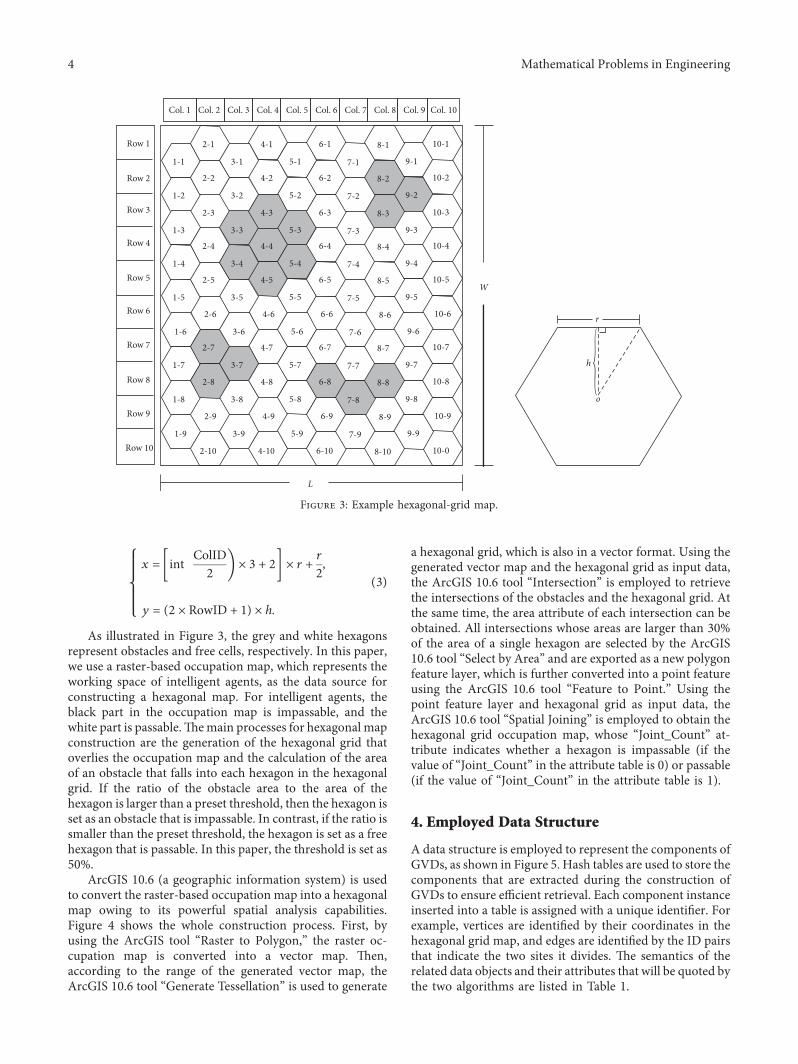

01
0S
S1
0
0
S0
10
10 0
S
0
0
1S
S0
10
(a)
10
1S
S0
1
1
S1
01
01 1
S
1
1
0S
S1
01
(b)
Figure 7 Patterns used by edge thinning (a) pattern one (b) pattern two
GenerateCrystalGrowthRoughGVDEdges()(1) while unCrystalCellListneOslash do(2) for all sbcl isin boundCellList do(3) for all s isin sbclcSiteCells do(4) for n isinAdj6(s) do(5) if typenneOBST then(6) if typen EMPTY then(7) typen⟵OCCUPY(8) obstn⟵ obsts(9) distn⟵ dists+ 1(10) insert(tempSBC cSiteCells n)(11) unCrystalCellListpop(n)(12) else if typen OCCUPY then(13) if obstnne obsts then(14) typen⟵EDGE(15) insert(newSBCL tempSBC)(16) boundCellList⟵ newSBCL(17) markCrystalRoughEdge()markCrystalGrowthRoughGVDEdges()(18) for all s isin allCellList do(19) if types EDGE then(20) e⟵ findEdge(s)(21) if e Oslash then(22) e⟵Edge()(23) obste⟵ obsts(24) insertEdge(e)(25) insertCell(e s)(26) insertQueue(roughQueue s dists)(27) pruningEdgeCell()
ALGORITHM 2 Pseudocode for the hexagon-based crystal-growth algorithm
Mathematical Problems in Engineering 9
and (2) the HCG algorithm is much more efficient andrequires less time than the hexagon-based Brushfire algo-rithm for each scenario with the same grid resolution
62 Application Test for Path Planning In order to dem-onstrate the usefulness of our algorithm for path planningtasks seven mobile robots operating in a fixed-size map with
(a)
(b)
Figure 8 Original raster map and seven hexagonal grid maps with different resolutions (a) First line left to right the original raster mapand grid maps with resolutions of 72times100 108times150 and 144times 200 (b) Second line left to right grid maps with resolutions of 180times 250216times 300 252times 350 and 288times 400
Table 2 Comparison of the computation time for seven hexagon-based GVD construction scenarios Construction from a fixed-size mapwith seven different resolutions
AlgorithmResolution
72times100 108times150 144times 200 180times 250 216times 300 252times 350 288times 400Hexagon-based Brushfire 75838 222965 516161 1116368 1820032 2946933 4481999Hexagon-based crystal growth 14945 35701 73051 147915 235950 374815 574377
pruningEdgeCell()(1) for all s isin roughQueue do(2) if fitPatternOne(s) or fitPatternTwo(s) then(3) continue(4) else(5) e⟵ findEdge(s)(6) eremove(s)thinningPatternOne(s)(7) for all n isinAdj6(s) do(8) if typen EDGE then(9) a b⟵ commonAdj(s n)(10) if typea EMPTY and typeb EMPTY then(11) return truethinningPatternTwo (s)(12) for all n isinAdj6(s) do(13) if typen EMPTY then(14) a b⟵ commonAdj(s n)(15) if typea EDGE and(16) (typeb EDGE or typeb OBST) then(17) return true
ALGORITHM 3 Pseudocode for obtaining one-cell-wide hexagon-based GVD edges using the two thinning patterns in Figure 7
10 Mathematical Problems in Engineering
seven different resolutions (shown in Figure 10) weresimulated+e starting points of the seven robots were at thesame absolute coordinates at the bottom left of the map Foreach search task each robot was given a unique destinationpoint with the same absolute coordinates at the top right of
the map However despite the same absolute coordinatesthe hexagonal grid coordinates of the seven starting pointswere different owing to the different resolutions +e gridcoordinates of the starting and destination cells of the sevenagents are listed in Table 3
(a)
(b)
(c)
Figure 10 (a) First line left to right hexagon-based GVD maps with resolutions of 180times 250 216times 300 252times 350 and 288times 400 (b)second line left to right path planning results adopting Alowast for entire hexagonal grid maps with resolutions of 180times 250 216times 300252times 350 and 288times 400 and (c) third line left to right path planning results adopting Alowast for hexagon-based GVDmaps with resolutions of180times 250 216times 300 252times 350 and 288times 400
Hexagon-based Brushfire algorithmHexagon-based crystal-growth algorithm
108lowast150 144lowast200 180lowast250 216lowast300 252lowast350 288lowast40072lowast100
Resolutions of maps (rowlowastcolumn)
00500
100015002000250030003500400045005000
Tim
e to
desti
natio
n (s
)
Figure 9 Comparison of the average computation time for constructing hexagon-based GVDs at different resolutions
Mathematical Problems in Engineering 11
+e search space adopted by these agents was (1) the entiregrid map and (2) the hexagon-based GVD metrics generatedby HCG +e Alowast algorithm was employed by the agents tosearch routes +e simulation results are listed in Table 4 Wecan see that the agents that adopted the Alowast algorithm to searchthe entire hexagonal grid map have a higher computation timeand more cell visits than those that adopted the Alowast algorithmto search the hexagon-based GVD metrics +e entire hex-agonal grid map provides no further information about themaximum clearance to sites making the resulting paths (inyellow in Figure 10) contain several cells near the sites whichwill lead to collisions when the physical size of the agentexceeds the limited clearance +e agents that adopted the Alowastalgorithm to search the hexagon-based GVD metrics onlyexplore the hexagon-based GVD edge cells significantly re-ducing the computation time Each of the resulting paths (inyellow in Figure 10) consists of (1) an initial route from thestarting cell to the nearest hexagon-based GVD cell (2) a set ofconnecting hexagon-based GVD edges ensuring the reach-ability of the hexagon-based GVD departure cell which isnearest the destination cell and (3) a final route from thehexagon-based departure cell to the destination cell +e pathplanning results of the seven simulation scenarios suggest thatthe ratio of the computation time for searching the whole mapwith the Alowast algorithm to that searching the GVD metricsincreases as the hexagonal grid resolution increases +e sameresult is also obtained for the ratio of the number of cells visitsfor searching the whole map with the Alowast algorithm to thatsearching the GVD metrics +is means that Alowast searching ofthe GVDs becomes more efficient than searching the entirehexagonal grid map as the hexagonal grid resolution increases
7 Conclusions
In this paper an algorithm named HCG was proposed toconstruct GVDs from hexagonal grid maps Several
simulation experiments were conducted to compare theHCG algorithm with the hexagon-based Brushfire algo-rithms (a leading grid-based GVD construction algorithm)and the results suggest that in a hexagonal grid map with thesame range and resolution the HCG algorithm is muchmore efficient requiring less time and fewer cell visits toconstruct hexagon-based GVDs Moreover two thinningpatterns for obtaining one-cell-wide GVDs from roughhexagonal GVDs were proposed and were applied to boththe hexagon-based Brushfire and HCG algorithms +eusefulness of the hexagonal GVD metrics in path planningwas further illustrated using several representative simula-tion scenarios and we found that it can significantly improvethe efficiency of path planning of intelligent agents
+e proposed HCG algorithm could be applicable to thepath planning of intelligent agents in fields of roboticscomputer games and military simulations where highcomputing performance needs to be guaranteed In thefuture a dynamic HCG algorithm will be further explored toefficiently construct GVDs from hexagonal grid maps inwhich local changes may occur
Data Availability
+e data used to support the findings of this study areavailable from the corresponding author upon request
Conflicts of Interest
+e authors declare that there are no conflicts of interestregarding the publication of this paper
Acknowledgments
+e authors wish to thank Jian Yang for his help in preparingthe manuscript+e authors would also like to thank Editage
Table 4 Comparison of the computation time and the average number of cell visits for path planning tasks performed by agents on bothwhole hexagonal grid maps and GVDs metrics with seven different resolutions
ResolutionWhole map GVD metrics Ratio
Time 1 (s) Cell visits 1 Time 2 (s) Cell visits 2 Time 1time 2 Cell visits 1cell visits 272times100 55708 3512 03591 1032 155132 34031108times150 181019 7463 06792 1550 266518 48148144times 200 542843 12926 12297 2221 441443 58199180times 250 1233430 20560 17734 2753 695517 74682216times 300 2362265 29340 29470 3537 801683 82951252times 350 4107248 38662 36282 4008 1132035 96462288times 400 6847620 51275 42549 4384 1609349 116959
Table 3 Grid coordinates of the starting and destination cells of the seven agents
Resolution Start cell (rowndashcolumn) Destination cell (rowndashcolumn)72times100 (70ndash3) (3ndash97)108times150 (105ndash4) (3ndash146)144times 200 (140ndash5) (3ndash196)180times 250 (176ndash6) (4ndash244)216times 300 (211ndash6) (4ndash293)252times 350 (247ndash7) (5ndash342)288times 400 (282ndash8) (6ndash392)
12 Mathematical Problems in Engineering
(httpwwweditagecn) for English language editing +isresearch was financially supported by Chinarsquos National KeyRampD Program (2017YFB0503500) and National NaturalScience Foundation of China (41901335)
References
[1] K Daniel A Nash S Koenig and A Felner ldquo+eta any-angle path planning on gridsrdquo Journal of Artificial IntelligenceResearch vol 39 pp 533ndash579 2010
[2] D Jia C Hu K Qin and X Cui ldquoPlanar waypoint generationand path finding in dynamic environmentrdquo in Proceedings ofthe 2014 International Conference on Identification Infor-mation and Knowledge in the Internet of4ings (IIKI) BeijingChina October 2014
[3] R M C Santiago A L De Ocampo A T UbandoA A Bandala and E P Dadios ldquoPath planning for mobilerobots using genetic algorithm and probabilistic roadmaprdquo inProceedings of the 2017 IEEE 9th International Conference onHumanoid Nanotechnology Information Technology Com-munication and Control Environment and Management(HNICEM) pp 1ndash5 Manila Philippines December 2017
[4] O Takahashi and R J Schilling ldquoMotion planning in a planeusing generalized Voronoi diagramsrdquo IEEE Transactions onRobotics and Automation vol 5 no 2 pp 143ndash150 1989
[5] R Klette and A Rosenfeld Digital Geometry GeometricMethods for Digital Picture Analysis Elsevier 2004
[6] J Barraquand and J-C Latombe ldquoRobot motion planning adistributed representation approachrdquo Tech Rep STAN-CS-89-1257 Computer Science Department Stanford UniversityStanford CA USA 1989
[7] N Kalra D Ferguson and A Stentz ldquoIncremental recon-struction of generalized Voronoi diagrams on gridsrdquo Roboticsand Autonomous Systems vol 57 no 2 pp 123ndash128 2009
[8] B Lau C Sprunk and W Burgard ldquoImproved updating ofEuclidean distance maps and Voronoi diagramsrdquo in Pro-ceedings of the 23rd IEEERSJ International Conference onIntelligent Robots and Systems (IROS rsquo10) pp 281ndash286 TaipeiTaiwan October 2010
[9] L Qin Q Yin Y Zha and Y Peng ldquoDynamic detection oftopological information from grid-based generalized Voronoidiagramsrdquo Mathematical Problems in Engineering vol 2013Article ID 438576 11 pages 2013
[10] I Her ldquoGeometric transformations on the hexagonal gridrdquoIEEE Transactions on Image Processing vol 4 no 9pp 1213ndash1222 1995
[11] L Middleton and J Sivaswamy Hexagonal Image Proc-essingmdashA Practical Approach (Advances in Pattern Recogni-tion) Springer Berlin Germany 2005
[12] E Luczak andA Rosenfeld ldquoDistance on a hexagonal gridrdquo IEEETransactions on Computers vol C-25 no 5 pp 532-533 1976
[13] T Lukic and B Nagy ldquoRegularized binary tomography on thehexagonal gridrdquo Physica Scripta vol 94 no 2 2019
[14] H J Quijano and L Garrido ldquoImproving cooperative robotexploration using a hexagonal world representationrdquo inProceedings of the Electronics Robotics and Automotive Me-chanics Conference (CERMA rsquo07) pp 450ndash455 MorelosMexico September 2007
[15] L Chrpa and A Komenda ldquoSmoothed hex-grid trajectoryplanning using helicopter dynamicsrdquo in Proceedings of the 3rdInternational Conference on Agents and Artificial Intelligence(ICAART rsquo11) pp 629ndash632 Rome Italy January 2011
[16] L Chrpa and P Novak ldquoDynamic trajectory replanning forunmanned aircrafts supporting tactical missions in urban
environmentsrdquo in Holonic and Multi-Agent Systems forManufacturing V Marık P Vrba and P Leitatildeo Eds vol6867 of Lecture Notes in Computer Science pp 256ndash265Springer Berlin Heidelberg 2011
[17] R M Mersereau ldquo+e processing of hexagonally sampledtwo-dimensional signalsrdquo Proceedings of the IEEE vol 67no 6 pp 930ndash949 1979
[18] L M de Sousa and J P Leitatildeo ldquoHex-utils a tool set sup-porting HexASCII hexagonal rastersrdquo in Proceedings of the3rd International Conference on Geographical InformationSystems 4eory Applications and Management pp 177ndash183Porto Portugal January 2017
[19] A Poorthuis and M Zook ldquoSmall stories in big data gaininginsights from large spatial point pattern datasetsrdquo Cityscapevol 17 no 1 pp 151ndash160 2015
[20] J P Morris ldquoAn application of multi-criteria shortest pathto a customizable hex-map environmentrdquo Masterrsquos thesisAir Force Institute of Technology Patterson OH USA2015
[21] Y Bjornsson M Enzenberger R Holte J Schaeffer andP Yap ldquoComparison of different grid abstractions forpathfinding on mapsrdquo in Proceedings of the Eighteenth In-ternational Joint Conference on Artificial Intelligence Aca-pulco Mexico August 2003
[22] J Wang M-P Kwan and L Ma ldquoDelimiting service areausing adaptive crystal-growth Voronoi diagrams based onweighted planes a case study in Haizhu district of Guangzhouin Chinardquo Applied Geography vol 50 pp 108ndash119 2014
[23] F Ricca A Scozzari and B Simeone ldquoWeighted Voronoiregion algorithms for political districtingrdquoMathematical andComputer Modelling vol 48 no 9-10 pp 1468ndash1477 2008
[24] O Aichholzer F Aurenhammer and B N Palop ldquoQuickestpaths straight skeletons and the city Voronoi diagramrdquoDiscrete and Computational Geometry vol 31 no 1pp 17ndash35 2004
[25] R Fabbri L D F Costa J C Torelli and O M Bruno ldquo2DEuclidean distance transform algorithms a comparativesurveyrdquo ACM Computing Surveys vol 40 no 1 pp 1ndash442008
[26] N S V Rao N Stoltzfus and S S Iyengar ldquoA lsquoretractionrsquomethod for learned navigation in unknown terrains for acircular robotrdquo IEEE Transactions on Robotics and Auto-mation vol 7 no 5 pp 699ndash707 1991
[27] H Choset S Walker K Eiamsa-Ard and J Burdick ldquoSensor-based exploration incremental construction of the hierar-chical generalized Voronoi graphrdquo 4e International Journalof Robotics Research vol 19 no 2 pp 126ndash148 2000
[28] CM Gold P R Remmele and T Roos ldquoVoronoi methods inGISrdquo in Algorithmic Foundations of Geographic InformationSystems M van Kreveld J Nievergelt T Roos andP Widmayer Eds vol 1340 of Lecture Notes in ComputerScience pp 21ndash35 Springer Berlin Germany 1997
[29] I Lee and M Gahegan ldquoInteractive analysis using Voronoidiagrams algorithms to support dynamic update from ageneric triangle-based data structurerdquo Transactions in GISvol 6 no 2 pp 89ndash114 2002
[30] S Scherer D Ferguson and S Singh ldquoEfficient C-space andcost function updates in 3D for unmanned aerial vehiclesrdquo inProceedings of the 2009 IEEE International Conference onRobotics and Automation (ICRA rsquo09) pp 2049ndash2054 KobeJapan May 2009
[31] T Y Zhang and C Y Suen ldquoA fast parallel algorithm forthinning digital patternsrdquo Communications of the ACMvol 27 no 3 pp 236ndash239 1984
Mathematical Problems in Engineering 13