
Heuristic algorithms for motion planning - PARC · Heuristic algorithms for motion planning Craig...
155
Heuristic algorithms for motion planning Craig Eldershaw Computing Laboratory The University of Oxford Hilary Term 2001
Transcript of Heuristic algorithms for motion planning - PARC · Heuristic algorithms for motion planning Craig...

Heuristic algorithms for motion planning
Craig Eldershaw
Computing Laboratory
The University of Oxford
Hilary Term 2001
Heuristic algorithms for motion planning
Craig Eldershaw, Keble College
Hilary Term 2001D.Phil. Thesis
Abstract
Motion planning is an increasingly important field of research. Factory automation is
becoming more prevalent and at the same time, production runs are shortening in the
name of customisation. With computer controlled equipment becoming cheaper and
more modular, setting up near-fully automated production lines is becoming fast and
easy. This means that the actual programming of the robots and assembly system is
becoming the rate determining step. Automated motion planning is a possible solution
to this—but only if it can run fast enough.
Many heuristic planners have been created in an attempt to achieve the necessary speeds
in off-line (or more ambitiously, on-line) processing. This thesis aims to show that
different types of heuristic planners can be designed to take advantage of specialised
environments or robot characteristics. To show this, three distinct classes of heuristic
planners are put forward for discussion.
The first of these classes, addressed in Chapter 2, is of very generic planners which
will work in virtually all situations (ie. almost any combination of robot and environ-
ment). This generality is obviously useful when lacking more specific domain knowl-
edge. However these methods do suffer performance-wise in comparison with more
specialised planners when there are characteristics of the problem which can be tar-
geted.
Chapter 3 moves to planners which are designed to specifically address certain peculiar-
ities of the environment. Particular focus is given to environments whose corresponding
configuration-spaces contain narrow gaps and passages.
Finally Chapter 4 addresses a third class of planners: those which are designed for
specific types of robots and movements. The particular focus is on locomotion for
legged vehicles.
For each of these three classes, some discussion is made of existing planners which can
be so characterised. In addition, a novel algorithm is introduced in each as an example
for particular consideration.
Contents
1 Introduction 11.1 Configuration space . . . . . . . . . . . . . . . . . . . . . . . . . . . . 41.2 Representation of the obstacles . . . . . . . . . . . . . . . . . . . . . . 81.3 Complexity . . . . . . . . . . . . . . . . . . . . . . . . . . . . . . . . 121.4 Heuristics . . . . . . . . . . . . . . . . . . . . . . . . . . . . . . . . . 131.5 Classes of planners . . . . . . . . . . . . . . . . . . . . . . . . . . . . 15
2 Generalised algorithms 172.1 Introduction . . . . . . . . . . . . . . . . . . . . . . . . . . . . . . . . 182.2 Genetic algorithms (GAs) . . . . . . . . . . . . . . . . . . . . . . . . . 22
2.2.1 Cross-over . . . . . . . . . . . . . . . . . . . . . . . . . . . . 242.2.2 Selection . . . . . . . . . . . . . . . . . . . . . . . . . . . . . 252.2.3 Mutation . . . . . . . . . . . . . . . . . . . . . . . . . . . . . 25
2.3 Previous motion planners employing GAs . . . . . . . . . . . . . . . . 262.4 Formulation . . . . . . . . . . . . . . . . . . . . . . . . . . . . . . . . 28
2.4.1 Overall form . . . . . . . . . . . . . . . . . . . . . . . . . . . 282.4.2 Constraint re-writing . . . . . . . . . . . . . . . . . . . . . . . 29
2.5 Why GAs? . . . . . . . . . . . . . . . . . . . . . . . . . . . . . . . . 312.6 This implementation . . . . . . . . . . . . . . . . . . . . . . . . . . . 32
2.6.1 Encoding . . . . . . . . . . . . . . . . . . . . . . . . . . . . . 332.6.2 Representation of the obstacles . . . . . . . . . . . . . . . . . . 332.6.3 Evaluation . . . . . . . . . . . . . . . . . . . . . . . . . . . . 352.6.4 Selection and cross-over . . . . . . . . . . . . . . . . . . . . . 372.6.5 Mutation . . . . . . . . . . . . . . . . . . . . . . . . . . . . . 38
2.7 Completeness, complexity and termination . . . . . . . . . . . . . . . . 382.8 Experimental results . . . . . . . . . . . . . . . . . . . . . . . . . . . 412.9 Parallelisation . . . . . . . . . . . . . . . . . . . . . . . . . . . . . . . 472.10 Optimal paths . . . . . . . . . . . . . . . . . . . . . . . . . . . . . . . 542.11 Dynamic planning . . . . . . . . . . . . . . . . . . . . . . . . . . . . . 552.12 Conclusion . . . . . . . . . . . . . . . . . . . . . . . . . . . . . . . . 56

3 Specialised environments 583.1 Planners that perform poorly . . . . . . . . . . . . . . . . . . . . . . . 593.2 Planners that succeed . . . . . . . . . . . . . . . . . . . . . . . . . . . 623.3 Overview of a new algorithm . . . . . . . . . . . . . . . . . . . . . . . 643.4 Constructing the new space . . . . . . . . . . . . . . . . . . . . . . . . 66
3.4.1 The primary obstacle lines . . . . . . . . . . . . . . . . . . . . 673.4.2 Overlapping obstacles . . . . . . . . . . . . . . . . . . . . . . 673.4.3 Boundary crossings . . . . . . . . . . . . . . . . . . . . . . . . 69
3.5 Calculating the path’s descent . . . . . . . . . . . . . . . . . . . . . . 703.6 Completeness, correctness, etc. . . . . . . . . . . . . . . . . . . . . . . 72
3.6.1 Termination . . . . . . . . . . . . . . . . . . . . . . . . . . . . 723.6.2 Correctness . . . . . . . . . . . . . . . . . . . . . . . . . . . . 733.6.3 Quality of path . . . . . . . . . . . . . . . . . . . . . . . . . . 743.6.4 Efficiency of execution . . . . . . . . . . . . . . . . . . . . . . 743.6.5 Completeness . . . . . . . . . . . . . . . . . . . . . . . . . . . 76
3.7 Implementation and results . . . . . . . . . . . . . . . . . . . . . . . . 783.8 Conclusion . . . . . . . . . . . . . . . . . . . . . . . . . . . . . . . . 82
4 Specialised modes of locomotion 844.1 Legged vehicles . . . . . . . . . . . . . . . . . . . . . . . . . . . . . . 854.2 Unstructured environments . . . . . . . . . . . . . . . . . . . . . . . . 864.3 PolyBot . . . . . . . . . . . . . . . . . . . . . . . . . . . . . . . . . . 874.4 Previous work . . . . . . . . . . . . . . . . . . . . . . . . . . . . . . . 89
4.4.1 Gaits for smooth-ground . . . . . . . . . . . . . . . . . . . . . 904.4.2 Foot-planners for broken ground . . . . . . . . . . . . . . . . . 914.4.3 Higher-level planners . . . . . . . . . . . . . . . . . . . . . . . 944.4.4 Shortcomings . . . . . . . . . . . . . . . . . . . . . . . . . . . 97
4.5 Splitting the planning work . . . . . . . . . . . . . . . . . . . . . . . . 994.6 The high-level path planner . . . . . . . . . . . . . . . . . . . . . . . . 101
4.6.1 CGspace . . . . . . . . . . . . . . . . . . . . . . . . . . . . . 1014.6.2 PRM . . . . . . . . . . . . . . . . . . . . . . . . . . . . . . . 1064.6.3 Combining PRM and CGspace . . . . . . . . . . . . . . . . . . 110
4.7 The foot-level planner . . . . . . . . . . . . . . . . . . . . . . . . . . . 1154.7.1 Heuristics . . . . . . . . . . . . . . . . . . . . . . . . . . . . . 1164.7.2 Comparisons with the free-gait . . . . . . . . . . . . . . . . . . 117
4.8 Modes of failure . . . . . . . . . . . . . . . . . . . . . . . . . . . . . . 1194.9 Parallelisation . . . . . . . . . . . . . . . . . . . . . . . . . . . . . . . 121
4.9.1 The high-level planner . . . . . . . . . . . . . . . . . . . . . . 1214.9.2 The foot-level planner . . . . . . . . . . . . . . . . . . . . . . 123
4.10 Example problem . . . . . . . . . . . . . . . . . . . . . . . . . . . . . 1234.11 Conclusion . . . . . . . . . . . . . . . . . . . . . . . . . . . . . . . . 125
5 Conclusions and Future work 127

Acknowledgments
I would like to take this opportunity to thank those people that made this thesis possible.
Thanks goes to Stephen Cameron, my supervisor at Oxford, for: providing many valu-able comments on drafts of this thesis; answering most of my silly questions; andvaliantly fighting the mound of paperwork which seems to accompany every student.
XEROX Palo Alto Research Center; their PolyBot crew generally; and Mark Yim inparticular dezerve (sic) a very big thank-you. Without them Chapter 4 would neverhave been written. The opportunity to “get my hands dirty” with hardware (much toStephen’s delight) was one I’m glad I had (though I may not have thought or said so atthe time !). More importantly, working as part of an energetic and friendly team was awonderful experience. I can only hope that I work with such a group at every workplaceI end up in.
Of course the very fact I’m in Oxford at all is due to the generosity of my fundingbody. My scholarship and university fees were paid by the Commonwealth ScholarshipScheme administered by the Association of Commonwealth Universities and the BritishCouncil. Several generations of kind people at these two organisations both ensured aregular supply of funds, and took the time and effort to ensure that I settled into Britishsociety.
“All work and no play makes Jack a dull boy”. . . and it doesn’t do much for his chancesof struggling through the ups and downs of doctoral life either. The many friends Icollected while in Oxford (mostly courtesy of the OU Walking Club) ensured that mynon-academic life was full of fun and companionship. Of these friends, two in particularstand out for special mention: Martin and Lydia Cordell. They: adopted me into thefamily; fed me wonderful food; tried to civilise me (. . . and failed, sorry guys); accepted(and returned) limitless amounts of teasing; gave me concrete to smash and mud to playin. What more could one ask of friends ?
Lastly (because I deferred writing this paragraph while trying to find the words), butmost of all, I have to thank my family. This is to all my family, but especially myparents, for their love, support, advice (asked for or not !) and encouragement. Withoutthat support this could never have happened. Thank-you.
To all these people: thank-you—I hope I’ve been able to give back something, to ex-press at least a fraction of my appreciation for what you’ve done.
CE .

Chapter 1
Introduction
Robot motion planning, according to Latombe’s well known book [65], is solving the
problem:
How a robot can decide what motions to perform in order to achieve goalarrangements of physical objects?
In many cases the physical objects that are to be arranged are simply the components of
the robot itself, though sometimes external objects are also to be manipulated. Implicit
in this definition is that the problem is subject to some constraints. These constraints
almost always include preventing collisions between the robot and obstacles in the en-
vironment. They may also include such things as bounds on velocity, acceleration or
torque.
Examples of situations where motion planning is used are many and varied.
Probably the two most commonly considered examples are: wheeled vehicles moving in
a two dimensional environment; and mechanically-actuated arms (manipulators). The
former arises in such situations as domestic or office robots that must move throughout a
building. Although these robots are likely have maps of the building’s floor-plans, they
must also support the possibility of other obstacles which will not be known in advance
(eg. people or displaced furniture). The motion planners in these robots must find routes

CHAPTER 1. INTRODUCTION 2
which move the robot from a point in the building to another without colliding with any
obstacles.
Mechanical arms most commonly arise in industrial settings, where manipula-
tors working on a factory assembly line must place, manipulate or fasten a component.
In these situations, a high degree of precision is usually required, but environmental
uncertainty is reduced as the component(s) are likely to be very close to the correct
position with no unforeseen obstacles intervening. Obviously the combination of these
is also possible: a mechanical arm mounted on a mobile wheeled base.
A problem related to manipulators is planning the motion of a hand or gripper.
Especially for the grasping of delicate objects, this is not just a matter of planning posi-
tions, but also the forces (sufficient to grasp the object in a stable configuration, but not
so much as to damage the object). A vastly more complicated problem is that of hand-
object manipulation (ie. repeatedly shifting the grasping configuration to manipulate
the object) [35, 101].
Other more specialised motion planning problems exist, and have been ad-
dressed in varying degrees by the literature. These includemovable obstacle problems
where the robot is able to move objects that form obstacles (eg. lift a piece of furniture
out of the way, or open a door) [24, 97]. Also themultiple movers problemwhere two
or more robots are moving in the same environment [31, 69]. In the simple case where
they each have independent goals, the planner just needs to ensure that the robots do
not interact adversely (eg. collide or block each other). More complicated versions of
this problem require the robots to actually cooperate (eg. two robots must hold opposite
corners of an object and carry it to a new location).
Most motion planning in current practical use falls into one of two clear cate-
gories. One of these is the use of mobile vehicles in uncertain environments where plans
must be made and updated in near real-time. In these cases, the need for rapid planning

CHAPTER 1. INTRODUCTION 3
(probably with limited on-board computational resources) has long been recognised
[14, 56]. Simpler variants of this which focus on the short-term planning are differ-
entiated from more general motion planning and are referred to asobstacle avoidance
algorithms.
Related to obstacle avoidance algorithms are temporal-based planners. In these
the environment is well defined, but varies with time. In these cases a location which is
free at one moment may not be the next. Some literature already exists which addresses
this: [33, 34, 58, 73].
The other main practical use of motion planning is the predominant one. This
is where the environment is well known, the task is to be planned once and then carried-
out many times. This is the case for assembly line robots.
However even in the case of the plan-once-execute-many-times situations, the
need for speed is still present—and indeed growing. When designing and preparing
an assembly line which will produce 10,000 cars over a 2 year period, one month of
computational planning time is acceptable (this can probably be overlapped with the
physical set-up of the plant). However smaller systems which are used for short runs
of customised products require little or no physical adjustment and so are slowed sig-
nificantly by the current performance of off-line motion planning. Such low-volume
systems appear to be on the increase, giving just one reason why motion planning algo-
rithms can still usefully be sped up.
Many different motion planning algorithms exist, some general (these will be
the focus of the next chapter), some for solving more specific problems like those men-
tioned above. Increasing in popularity these days are algorithms which are heuristic
(discussed in Section 1.4). A number of these will be reviewed in some detail in each
of Sections 2.1, 3.1, 3.2 and 4.4.

CHAPTER 1. INTRODUCTION 4
1.1 Configuration space
A motion-planner needs to be constantly aware of where all parts of the robot are.
For example in a car, it is not sufficient to ensure that the driver’s side front corner
makes it through a gate if the passenger’s side mirror gets broken off. Of course the
problem is compounded if the vehicle isn’t a rigid body (for example an articulated
truck). This constant testing of all parts of the vehicle against near-by obstacles becomes
very awkward—especially with more complicated vehicles or environments.
A solution to this has been devised: the concept ofConfiguration Space(or
C-space) [68]. The number of dimensions in C-space corresponds to the number of
degrees of freedom of the robot, not the number of dimensions in the real environment.
The volume and shape of the vehicle is “added-on” to each of the obstacles. The ve-
hicle’s representation in this new space is simply a point. Each point in configuration
space corresponds to a particular configuration of the vehicle and exactly describes its
location and orientation with respect to the environment.
To state this more formally:
Let W ⊂ R3 be the workspace—the region the robot moves about in.
Let R be an abstract description of the robot.
Let R : (R × Rd)→ PW be a function that maps thed dimensional configuration of
a robotR to a region of the workspace occupied by the robot in that configuration.
TheRd typically includes the location of the robot (in practice, the location of a chosen
reference point on the robot in some Cartesian space) and its orientation (or in the case
of manipulators, the angle and length of each of the manipulator’s segments).
Let Oi ⊂ R3 be the workspace obstacles—those regions of the workspace that no part
of the robot may occupy.

CHAPTER 1. INTRODUCTION 5
Then the C-obstacles are
Ci(R)={p ∈ Rd|R(R, p) ∩Oi 6=∅}
These are sets of configurations that the robot must not adopt due to intersection with
obstacles. Note that this is a function ofR; ie. the same environment with a different
robot will have different C-space obstacles.
Finally, the full configuration space is
CSpace(R)=⋃i
Ci(R) ∪ {p ∈ Rd|outOfRange(R, p)}
whereoutOfRange(R, p) : (R × Rd) → {True,False} returnsTrue if the given con-
figuration exceeds some internal limits of the robot (eg. restrictions on joint range) or
will lead to self-intersection.
Figure 1.1 shows how a translating robot’s shape can be added to that of the
obstacles to produce enlarged obstacles (shown as dashed lines). Once the C-space is
formed, the vehicle’s shape can be dismissed—it is now represented by a single point
corresponding (in this case) to the upper-left corner of the vehicle. If that point remains
outside all of the configuration-space obstacles, then the robot has not collided. In this
particular example, it can be seen that the C-space obstacles actually overlap, preventing
movement of the robot’s reference point between them. This corresponds to the fact that
(without rotation) the vehicle cannot fit through the gap between the original obstacles.
As stated earlier, the dimensionality of C-space is equal to the number of de-
grees of freedom of the vehicle. So if the vehicle is allowed to rotate within a two
dimensional environment, then the resultant C-space is three dimensional (two spatial,
one rotational). Again, the representation of the vehicle is simply a point corresponding
to some position and orientation of the robot. If this point (which is now free to wander

CHAPTER 1. INTRODUCTION 6
Vehicle
Obstacle
Obstacle
PointReference
Figure 1.1:This figure shows how the shape of the vehicle can be “added” to that ofthe obstacles to yield the configuration space equivalent of the given envi-ronment.
in a three dimensional space) remains clear of all the configuration space obstacles, then
the entire vehicle is clear of all of the obstacles. A cross-section of this three dimen-
sional space atz = c would be a plane (parallel to thex–y plane) corresponding to the
configuration space that would exist if the orientation of the vehicle were fixed atc.
An extension to this is the case of mechanical arms or manipulators. Move-
ment in these situations is not simply a case of translation or rotation of the entire
apparatus, but of each part individually. For example take a three-segment mechanical
arm which lies in a plane: one end is fixed, and the other free to move to wherever the
combination of the three angles holds it. These three joints, managed by the controller,
can be treated as a three degree of freedom system; and so can be mapped to a three
dimensional C-space. The fact that all three of these dimensions are rotational and not
translational is irrelevant once the problem has been transformed. A consideration in
motion-planning for robot manipulators, is that the manipulator may self-intersect (ie.
the arm might bend around far enough that it hits itself). Clearly this is to be avoided,
and once again, C-space solves the difficulty. By simply placing obstacles in regions
of the C-space which correspond to such self-intersections, then all computer generated
paths of motion will avoid those configurations.

CHAPTER 1. INTRODUCTION 7
A very useful extension of the notion of configuration-space isconfiguration-
time space. This can greatly simplify the planning in time-varying problems. If the
obstacles in a problem are allowed to move around, then the detection of collisions
between vehicles and obstacles becomes considerably more difficult. At each time that
such tests are to be performed, the current location and orientation of all obstacles must
be determined. Furthermore, care must be taken that a collision does not occur in the
interval of time between two such tests (both of which could indicate that the robot is
clear of obstacles at these two points in time).
A lot of these difficulties can be prevented and the problem made conceptually
much cleaner by subsuming these time-dependencies into an additional temporal di-
mension of the configuration-time space. Figure 1.2 shows (on the left) a C-space with
two configuration space obstacles (CSOs)—a moving square and a stationary triangle.
On the right is shown the configuration-time space that results from it. The triangle is
identical in any cross-section made atTime = τ . However the square (moving in the
positivex direction, becomes a parallelepiped sloping in the positivex direction. Any
position outside of these two three dimensional obstacles is in free spaceat whatever
moment in time that happens to be. In this new space, a normal (non-temporally aware)
planner can be applied. The main additional limitation that must now be applied to the
path is that its route must be monotonically increasing in the temporal dimension. In
addition velocity bounds may be required: these take the form of limiting the angle the
path can take in the new dimension.
So C-space allows abstraction from many of the more complicated aspects of
the environment by transforming them such that they can all be treated in the same
manner (ie. location, orientation and time-dependence all become equivalent). Note
that while this abstraction is convenient for restating the problem, the construction of
C-space is itself quite expensive, both in terms of computation time and storage space.
The later is particularly prevalent in multi-jointed dextrous robots which have many

CHAPTER 1. INTRODUCTION 8
Moving Stationary �
� �
�
��
��
CSO CSO
Figure 1.2:This figure shows how motion of objects (and their associated configurationspace obstacles—CSOs) can be absorbed into C-space by adding a tempo-ral dimension.
degrees of freedom, since storage space is usually exponential ind. Exactly how this
storage problem arises and is addressed in the literature is the topic of the next section.
For a survey of some of the available algorithms for generating C-spaces, see [46] and
[65].
1.2 Representation of the obstacles
Closely tied with the notion of C-space is the means of representing and storing obsta-
cles. Every planning algorithm needs the original space to be stored, either for direct
access, or for indirect access through requests for C-space materialisation. Then too, the
materialised C-space (if the algorithm uses C-space) must be returned to the planner in
some form or other. Of course to run the program in the first instance the data describ-
ing the environment must be made available in some form. So there are in fact up to
three distinct forms of the environment that may need to be considered: the input form
of the environment; the actual stored form; and the form of the constructed C-space.
The first of these—the input form of the environment—is usually not going to
be the choice of the planner’s designer. It will be whatever is provided in the particular
circumstances in which the planner is required. This may be something which exists in

CHAPTER 1. INTRODUCTION 9
a nice easy-to-process form like a geometrical model or bitmap, however it could also
be sensor data. Many robots have some kind of sensor system which can provide such
input as image data or one dimensional sonar maps. Obviously data in these forms will
need some processing—it cannot be used raw.
The third form of the environment—the C-space returned to the planner—will
be decided largely by the choice of planner. This is particularly the case with planners
that are designed to work very closely with the environment’s obstacles in some partic-
ular representation. This is the case for several of the planners discussed in Chapter 3.
Clearly the dictates of such planners must be met. In contrast, some planners are rel-
atively divorced from the environment—the genetic algorithm based method discussed
at length in Chapter 2 is one of these. Rather than deal with the environment or C-
space directly, Chapter 2’s algorithm treats the environment as a “black-box” to which
it periodically issues queries as to whether a path it has proposed is collision-free.
In between these two, is the storage layer. In what form is the planning system
going to store the information? It may choose to keep it in the initial input form, or
to process it directly to the form required by the planning algorithm, or it may use
some intermediate format. Many different approaches have been tried; each with their
various merits (storage space, processing requirements, accuracy, etc.). Some of these
are discussed below.
It is straight-forward to simply store an exact geometric description of the ob-
stacles. Each obstacle is decomposed into a set of basic elements (lines and curves)
which can then be described by a simple listing of the components. This also tends
to make for a very compact representation. Sometimes the representation is simpli-
fied further by using only straight lines; in this case curves must be approximated by
collections of straight line segments.
The advantages of compactness and exactness are obvious, unfortunately the
CHAPTER 1. INTRODUCTION 10
cost is paid in the form of processing. Geometric calculations (a large number of which
are required by the planner) are notoriously expensive—especially in the higher dimen-
sions that C-spaces often are. If the environment is something like a factory floor—for
which CAD drawings will exist—then generating these geometric forms in the first in-
stance is simple. However in other situations, some or all of the information about the
environment is derived from sensor readings and cannot readily be converted into this
exact form.
At the opposite extreme is the use of bitmaps. This is where the entire environ-
ment is discretised and each cell is assigned a binary value: zero for free space, one for
occupied (whether in part or in whole) by an obstacle. This discretised space can then
be searched using various techniques, a number of which are explored in [4]. These
bitmap representations suffer from two potentially significant disadvantages. One of
these is storage size—which can be very large as it is potentially exponential in the
dimensionality of the C-space. The second is the closely related problem of determin-
ing the correct resolution. An excessively fine discretisation is costly in memory and
computation, however too coarse a resolution prevents important fine details from being
correctly represented. This is especially of concern when the C-space contains narrow
passages. This difficult situation will be the focus of Chapter 3.
These joint concerns of memory and choice of resolution are partly addressed
for the case of two dimensional problems in [34], where it is suggested that quad-trees
are used to represent the space. This is a nice compromise which effectively allows
the resolution to vary across the domain as needed. Where there is a large compact
region of either free space or solid obstacle then little memory is used. In those regions
with fine detail, more memory is used. With some additional complications of the data
structures, this idea can be extended to higher dimensions: in three dimensions there
are oct-trees [58] and more generallykd-trees [85, 86].
Rather than decomposing C-space into squares/cubes/hyper-cubes for storage

CHAPTER 1. INTRODUCTION 11
and processing, some authors have instead chosen sphere hierarchies [78]. Spheres
have the great advantage of being very efficient to use in geometric calculations. For
this reason, as will be elaborated in Section 2.6.2, they were chosen as the preferred
representation for the algorithm introduced in Chapter 2.
Another approach is to only store one representative path-fragment from each
family of such fragments. Afamily of paths is a set such that any one path can be
deformed to become one of the others without causing the path to pass through a C-
space obstacle at any stage of this transition—ie. they are all topologically equivalent.
Particular versions of this which are commonly used are the Voronoi and silhouette
methods [17]. The Voronoi method chooses its representative path fragments so as to
always be equidistant from all nearby obstacles. This means that the resulting path gives
all obstacles a wide-berth—a very useful property for a practically usable path.
An interesting alternative put forward in [13] is to represent the majority of
free-space as generalised cones. Unfortunately the work currently only supports rigid
bodies (ie. vehicles, not manipulators) in a relatively open two dimensional workspaces.
The paths generated by this algorithm follow the axes of these cones, and so again have
the desirable property of keeping the vehicle well away from the obstacles. These will
be discussed in a more detail in Section 3.1.
The means of representing the environment discussed so far are either for gen-
eralised C-space or (in the case of the generalised cones) for standard obstacles in a
workspace. However for some problem domains, different information concerning the
environment is required. As with general program design, choice of data-structures
must be considered in the context of the queries made of it. The chief examples of this
are such problems involving unstructured terrains. Here the information required is the
height, slope and frictional coefficients of the entire work surface. For practical prob-
lems of this kind, there is no real way to store this information except as one (or more)
two dimensional arrays. Height-maps of this kind will be discussed in some detail in
CHAPTER 1. INTRODUCTION 12
Chapter 4.
1.3 Complexity
Complexity can be considered in two components: computational time-complexity and
storage complexity. Time-complexity partitions algorithms into the overlapping classes:
P (can be solved in polynomial time), NP (can be verified in polynomial time), NP-
Hard (can be reduced to an NP problem in polynomial time—ie. is at least as hard
as any NP problem) and NP-Complete (both NP and NP-Hard). The storage equiva-
lents are PSPACE (for algorithms whose storage requirements are polynomial in the
degree of the problem), PSPACE-Hard (if every problem in PSPACE is polynomial-
time reducible to the given problem) and PSPACE-Complete (in PSPACE-Hard and in
PSPACE).[76]
The complexity of motion planning cannot be simply stated as there is no one
standard problem to be examined (as opposed to other fields in computer science which
do—eg. matrix multiplication in linear algebra). Indeed even theGeneralised Mover’s
Problem(the closest the field has) has slightly inconsistent definitions in the literature.
In addition there is not just one, but in fact two significant variables in the case of motion
planning: dimensionality (the number of degrees of freedom that the robot has) and the
size of the environment (the number and/or degree of the obstacles).
However there do exist some results for a few very specific problems. Moving
a convex polyhedron amongst a finite number of polyhedral obstacles is PSPACE-Hard
[83]. The time complexity for planning the motion of a robot with a fixed number
of degrees of freedom amongst stationary obstacles is polynomial in the number of
obstacles. However it is exponential in the degrees of freedom [17]. In [84], Reif and
Sharir prove that the time complexity of the two dimensionalmovingobstacle problem

CHAPTER 1. INTRODUCTION 13
is polynomial—provided that the number of obstacles is bounded and that their speed is
less than that of the robot. At higher obstacle speeds, this becomes NP-Hard. Shortest
path planning (ie. not just feasibility but some kind of optimality of path) is NP-hard
[17]. For detailed complexity results on some aspects of motion planning, see [17] and
[87].
It should be noted that most of the algorithms used to prove these complexity
bounds are not intended for practical use. While their theoretical complexity may be
low, the multiplicative constants in the computation times are for the most part suffi-
ciently high as to render the algorithms uncompetitive for use on any reasonable sized
problem.
Since the focus of this thesis is upon practical heuristic algorithms where com-
plexity analysis is not particularly relevant, then it will largely be ignored for the re-
mainder of this thesis except for Sections 2.7 and 3.6.4.
1.4 Heuristics
According to [43], aheuristicis:
A rule of thumb, simplification or educated guess that reduces or limits thesearch for solutions in domains that are difficult and poorly understood.Unlike algorithms, heuristics do not guarantee optimal, or even feasible,solutions and are often used with no theoretical guarantee.
That is, they are algorithms that do not guarantee to find a solution, but if they do, are
likely to do so much faster than the competing complete methods. They frequently work
by performing a series of (sometimes non-deterministic) refinement steps which will
hopefully converge upon a feasible (though not necessarily optimal) solution. The fact
that a heuristic algorithm has failed to solve a particular problem does not necessarily
mean that there is no solution to that problem, or even (given that some heuristics are
non-deterministic) that re-running the algorithm will result in failure again.

CHAPTER 1. INTRODUCTION 14
In the case of motion planning, the space of possible paths to be searched is
theoretically infinite. In practice however, the C-space is always discretised, whether
deliberately through a coarse cell-based approximation, or implicitly by the finite res-
olution imposed by the fixed storage space for a floating point number. In the latter
case this “finite” search space is far too large to contemplate a complete search, and
for large problems even an explicitly discretised domain is likely to be vastly greater
than can feasibly be searched completely. However in any case, one of the fundamental
aspects of any algorithm is to choose somefiniterepresentation of the problem (whether
generalised cones, or Voronoi roadmaps, etc.) to make the problem solvable.
When discussing completeness in the context of heuristic algorithms, then two
weaker forms of completeness should be considered. The first of these isresolution
completeness. This term arises when a continuous problem has been discretely approx-
imated in preparation for applying a planning algorithm. If the algorithm is complete
for the approximation to the environment given but there is some risk that the resolu-
tion of the approximation is such that it has incorrectly captured critical details of the
problem, then the situation can be considered resolution complete. Examples of this are
discussed in Section 2.1.
The termprobabilistic completenessis applied to a heuristic algorithm that is
complete (in that it is guaranteed to find a solution should one exist), but has no upper
bounds on the total complexity. That is, as computation effort expended increases, so to
does the probability of successful completion. The limiting case (where the probability
reaches the level of certainty) occurs only as computational effort (or, in practical terms,
computation time) approaches infinity. While the monotonically increasing probability
of success is nice, the limiting case proves rather cold comfort in practice. Probabilistic
completeness is discussed further in Section 2.7.
A further argument for heuristic approaches (as opposed to the more satisfying
complete planners) is that the problem itself may not be precisely defined. In the partic-

CHAPTER 1. INTRODUCTION 15
ular case of planning, this usually arises in the accuracy of knowledge of the environ-
ment. If the input environment is inaccurate, then this will place a limit on the validity
of any solution found (or not, as the case may be) anyway. Knowledge of environments
arises from one of two ways. It can be sensed (directly by lasers, sonar, vision-systems,
etc.; or indirectly when someone measured the environment and entered the details into
the planning system), in which case measurement errors are inevitable. Alternatively
(as is often the case in industrial settings) the environment was designed from a precise
computer-based design, and so this is fed to the planner as the robot’s environment—in
this case the inevitable errors are not in measurement, but in construction.
As explained in the introduction to this chapter, a key issue for motion plan-
ning is increasingly becoming the speed of such planning. The complete algorithms
mentioned in the previous section are guaranteed to solve the problem (though often
only for very specialised situations—not the full generalised movers problem), how-
ever the time taken is not practical in many situations. So heuristic methods seem to
have been generally accepted by the research community as the direction to pursue for
designing efficient practical planners.
1.5 Classes of planners
This thesis attempts to show that different types of heuristic planners can be designed
to take advantage of specialised environmental or robot characteristics. To show this,
three distinct classes of heuristic planners are put forward for discussion.
The first of these classes, addressed in Chapter 2, contains very generic plan-
ners which can be successfully applied to virtually any situation (ie. almost any com-
bination of robot and environment will result in a solution if one exists). The merits of
a number of existing planners including: cell-based planners, potential-based planners,

CHAPTER 1. INTRODUCTION 16
and the probabilistic road-map planner are discussed. Then a novel planner employing
genetic algorithms is investigated at some length. The generality of these planners is
obviously useful when lacking more specific domain knowledge. However these meth-
ods do suffer with regards to performance in comparison with more specialised planners
when there are characteristics of the problem which can usefully be targeted.
Chapter 3 introduces the concept of these more specialised planners. Specifi-
cally it considers planners that work effectively in environments whose corresponding
C-spaces contain narrow gaps and passages. Firstly the effectiveness of existing plan-
ners (such as: the randomised path planner, a generalised-cones based planner, Voronoi
planners and visibility graph planners) is discussed, and then a new planner which di-
rectly addresses the problem is described.
Finally Chapter 4 addresses a third class of planners: those which are designed
for specific types robots and movements. The particular focus in this chapter is on
locomotion for legged vehicles in unstructured environments. Comprehensive practical
algorithms in this area seem particularly scarce. The approaches taken by those which
do exist (including such direct methods as simply randomly sampling from all possible
paths) are considered, then a new algorithm incorporating a number of unique features
is introduced.

Chapter 2
Generalised algorithms
The aim of this thesis is to show that specialised heuristic algorithms can be tailored
for particular environments or robots. However sometimes too little is known about an
environment in advance or the C-space contains no exploitable features. In these cases
a generalised planner is the only way forward. This chapter discusses several existing
planners and introduces a novel, completely general planner.
The algorithm put forward here expands upon the work described in [28] and
[29]. It works by reformulating the problem of motion planning as one of optimi-
sation, and then employs genetic algorithms to do this. Approaching the problem in
this way achieves several benefits. Two key benefits are its probabilistic completeness,
and its relative independence from the environment’s representation. Furthermore, this
algorithm (as with many genetic algorithms) is quite amenable to parallelisation. The
author’s implementation has been parallelised and the efficiency of this is demonstrated.

CHAPTER 2. GENERALISED ALGORITHMS 18
2.1 Introduction
Most existing C-space-based planning algorithms are relatively general in nature. A
good review of the these is to be found in [65] or the more recent [46]. This chapter’s
main example is a new genetic algorithm-based approach. To give some perspective,
this section will review a number of existing competing algorithms.
In Section 1.2 the concept of storing the C-space as uniform cells was dis-
cussed. This representation is integral to a number of planning algorithms [82, 89, 98].
Many of them work by searching the structure from start to finish according to some
heuristic (see [4] for a survey of these).
1011
12
567 8
42
9
1
F
S
30292827 26 25
24 2322 21
2019 18 17
1615 14 13 3
Figure 2.1:A best-first search through a 2D C-space represented as cells
Figure 2.1 shows an example of a best-first search. The starting cell (marked
“S”) is considered cell 0. Each of its four-adjacent neighbours is considered, and of
those which are free (in this case all of them), the one closest (in a Euclidean sense) to
the finish is selected and numbered 1. Cell number 1’s neighbours are now considered
as well(ie. all free unnumbered cells adjacent to numbered cells are now considered).
The best (ie. closest to the finish) of all these is selected and labelled 2. This is repeated
until the cell containing the finish is reached. Now the algorithmbacktracksthrough
CHAPTER 2. GENERALISED ALGORITHMS 19
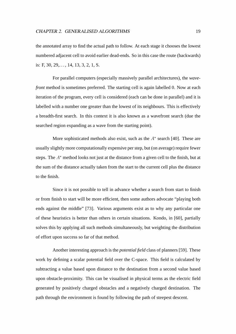
the annotated array to find the actual path to follow. At each stage it chooses the lowest
numbered adjacent cell to avoid earlier dead-ends. So in this case the route (backwards)
is: F, 30, 29,. . . , 14, 13, 3, 2, 1, S.
For parallel computers (especially massively parallel architectures), thewave-
front method is sometimes preferred. The starting cell is again labelled 0. Now at each
iteration of the program, every cell is considered (each can be done in parallel) and it is
labelled with a number one greater than the lowest of its neighbours. This is effectively
a breadth-first search. In this context it is also known as a wavefront search (due the
searched region expanding as a wave from the starting point).
More sophisticated methods also exist, such as theA? search [40]. These are
usually slightly more computationally expensive per step, but (on average) require fewer
steps. TheA? method looks not just at the distance from a given cell to the finish, but at
the sum of the distance actually taken from the start to the current cell plus the distance
to the finish.
Since it is not possible to tell in advance whether a search from start to finish
or from finish to start will be more efficient, then some authors advocate “playing both
ends against the middle” [73]. Various arguments exist as to why any particular one
of these heuristics is better than others in certain situations. Kondo, in [60], partially
solves this by applying all such methods simultaneously, but weighting the distribution
of effort upon success so far of that method.
Another interesting approach is thepotential fieldclass of planners [59]. These
work by defining a scalar potential field over the C-space. This field is calculated by
subtracting a value based upon distance to the destination from a second value based
upon obstacle-proximity. This can be visualised in physical terms as the electric field
generated by positively charged obstacles and a negatively charged destination. The
path through the environment is found by following the path of steepest descent.

CHAPTER 2. GENERALISED ALGORITHMS 20
This is a very efficient method. Barring local minima, then each iteration of
the algorithm monotonically extends progress along a path to the destination. While
theoretically a full implementation of this would require the influence of alln obstacles
to be calculated at each step, in practice only those in the near vicinity need be consid-
ered (the inverse-square law of electrostatics makes the effect of more distant obstacles
negligible).
The disadvantage with this approach is that local minima in the potential field
are easily produced, causing the search to terminate before reaching the required desti-
nation. This is addressed in [5] and [6] where a random walk is performed to “escape”
any local minima. In many ways this method is reminiscent of thesimulated anneal-
ing methods [9, 25] for function minimisation in the presence of local optima. Other
authors have adopted variations upon this [19, 20].
One other method related to cell-based representation is particularly worthy of
mention. Keymeulen and Decuyper in [57] also borrow ideas from physical models. In
this algorithm the environment is treated as a sealed system with a non-viscous fluid
flowing from a point source placed at the required starting point to a point sink at the
robot’s destination. The path returned is any of the stream-lines connecting these two
points. Cell-based representation is common in fluid dynamics simulations, though
often the fixed sized cells of the previous methods are replaced by variable sized ones.
All these cell-based methods are (at best)resolution-complete. This means
that if the resolution is such that the decomposition of the C-space correctly captures all
the required passages, then the solution will be found. Unfortunately uncertainty arises
through the possibility of a critical narrow passage being artificially blocked as demon-
strated in Figure 2.2. This problem can of course be avoided by reducing the resolution,
but doing so is costly, and simply finding the maximum safe size may expensive in
itself.

CHAPTER 2. GENERALISED ALGORITHMS 21
Figure 2.2:The two grey obstacles artificially segregate the free space due to the cellresolution chosen.
The visibility method of Kant and Zucker [53] is aroadmapmethod—ie. one
where the obstacle-free regions of C-space are represented by a series of edges (“roads”)
which are later searched through. In this case, the visibility graph method constructs a
graph of every feasible straight line (ie. one that penetrates no obstacles) that connects
two obstacle vertices. This becomes rather expensive in higher dimensional environ-
ments; furthermore it requires that the C-space be available in an exact representation.
However it does have some useful properties—for this reason the algorithm will be
explored more in the next chapter in Sections 3.2 and 3.6.4.
One method that has proved very successful in practice is theprobabilistic
roadmap method[55] (or PRM). In this method random points are scattered throughout
the C-space. If any pair of points (selected from either the randomly generated ones and
the given start/end points) are considered sufficiently close, then an attempt is made to
join them with a cheap local planner. A graph is maintained with each of the above-
mentioned points corresponding to a node, and edges in the graph corresponding to a
successful local connection. When the start and end nodes are finally within the one
connected component of the graph, then the planner has been successful. In later stages
of the algorithm, certain heuristics can be applied to improve point placement based

CHAPTER 2. GENERALISED ALGORITHMS 22
upon previous successes and failures. This method will be addressed in more detail in
Section 4.6.2.
Several authors have suggested that techniques from optimisation theory be
applied to the motion planning problem. Tominaga and Bavarian in [92] have an inter-
esting approach that is discussed in Section 3.2. Apart from this and the potential field
planners mentioned earlier, most optimisation based motion planners employ genetic
algorithms. The next section gives an overview of how genetic algorithms work in gen-
eral, and the one following that (Section 2.3) describes existing genetic algorithm-based
techniques for motion planning.
2.2 Genetic algorithms (GAs)
To understand the rest of this chapter, it is necessary to understand something of how
genetic algorithmswork; this section provides a brief overview. GAs were initially
developed by Holland [42]. For a more detailed treatment, the interested reader is
referred to the many works available in the literature, including [21, 37, 72].
There exist many different kinds of optimisation algorithms: some exact, some
heuristic. Some optimisation problems are amenable to algebraic solutions, but in gen-
eral these are either impractical (due to computational expense), or outright impossible.
Other exact methods are applicable only to certain classes of problems (eg. linear pro-
gramming). The heuristic methods are generally much faster than their analytic counter-
parts, however they: (a) may not converge to an exact solution (though they can usually
find a solution to any requested accuracy); and (b) may not find the global minimum.
Most practical optimisation problems do not have a single minima, but rather
several. For some purposes, an algorithm which reports any of these local minima is
adequate. However it is often the case that the problem’sglobal minimum is required.

CHAPTER 2. GENERALISED ALGORITHMS 23
Unfortunately this is a much harder problem to solve—in fact in the general case (where
the minimum value that the function attains is not known), it is intractable.
GAs belong to the class of what is known asglobal optimisation algorithms.
These global optimisation algorithms are specifically designed to attempt to find the
global minimum of the input function rather than just an arbitrary local minimum. The
other best known global optimisation technique is that of simulated annealing (previ-
ously mentioned in Section 2.1 in connection with the randomised path planner [6]).
Opinions vary widely as to the relative merits of GAs and simulated annealing. For one
such comparison, see [26].
GAs are so called since they are modelled loosely upon the biological process
of natural selection. They form successive populations of individual solutions to the
problem. The algorithm attempts to improve the quality (referred to asfitnessin the
GA context) of these individuals from generation to generation. The change in the
population is achieved by the selection, reproduction and mutation procedures within
the method. The selection operation is dependent upon the fitness of the individuals
concerned.
GAs are characterised by the fact that all the information on any individual
solution in the population is encoded using a linear encoding system. This (usually
binary) encoding is intended to be somewhat analogous to natural DNA (which is a
long sequence consisting of four kinds of chromosomes).
The standard encoding technique for applying genetic algorithms to non-linear
optimisation problems with continuous and real parameters, is a concatenation of all the
binary approximations to each number. As an example: if the function to be maximised
was of two variables(x1, x2), with the domain of each being[0, 10] and required accu-
racy at least0.01, then each of these variables would be encoded by 10 bits. In more
detail: a 10 bit binary string can take on210 =1024 ≈ 1000 distinct values. By interpret-

CHAPTER 2. GENERALISED ALGORITHMS 24
ing this string as an integer from0 to 1023 then a discrete approximation to100x1 has
been formed. This can be repeated to encode the second variable in a similar manner.
Then, by concatenating the two 10 bit strings to yield a 20 bit string, a single genetic
string can be formed to represent both parameters.
With the exception of the fitness evaluation, no operation within the algorithm
has any knowledge of the encoding method or number of variables. Whenever the
fitness of a gene is to be evaluated, a routine must decode the bit string (ie. get(x1, x2)
back again) and evaluate the fitness function with(x1, x2) as input. This then gives
the fitness of the individual to be used in the genetic algorithm. A higher function
evaluation indicates a higher level of fitness of a particular genetic string—ie. a “better”
solution.
Having arrived at a consistent reversible encoding method and knowing that
the initial population is randomly chosen, what remains is how to perform the changes
from one “generation” to the next. It is achieved by a combination of three procedures,
cross-over, selection and mutation.
2.2.1 Cross-over
Cross-overis the means by which two different genetic strings (ie. members of the
population) can combine to form two new “offspring”. One common method is to
choose a random place to “cut” the two bit strings (the same place for both). Then
by combining the first section of the first string with the second section of the second
string, a new string is formed—inheriting some characteristics from each of its parents.
A more more elaborate method of combining two genes is known as 2-point
cross-over (the previously discussed method is called 1-point cross-over). This is per-
formed by cutting both the gene strings at not just one place, but at two places each.
The new string is formed by combining the first and last sections of the first string with

CHAPTER 2. GENERALISED ALGORITHMS 25
the middle section of the second.
Yet another method for re-combination is known asuniform cross-over. Uni-
form cross-over is achieved by creating a random bit mask of the same length as the
gene strings. The new string is formed by taking the value in thenth position of the first
string if thenth value of the mask is a 1, otherwise taking the value in thenth position
of the second string.
2.2.2 Selection
This is one of the most important of the GA operations. This is where it is decided
which members of the population will be allowed to survive, and which will perish.
It is usually done via a weighted random selection where the weighting is based upon
the fitness of each individual. That is, the more fit members of the population have a
greater chance of progressing to the next generation than those less fit. This selection
process (or some slight modification of it) is used to select pairs of parents which will
“mate” (using the cross-over methods discussed above) to give offspring to replace the
deceased ones.
2.2.3 Mutation
While opinions differ as to the exact goal and importance of mutation, the means by
which it is carried out is usually agreed upon. Basically each bit within the gene string
is flipped with a certain (very small) probability. This probability is usually less than one
in a thousand. Some authors propose that the mutation is simply a means of preventing
an early convergence (and hence allowing the algorithm enough time to complete its
work). However others claim that it is, in fact, an essential means of introducing genetic
diversity into the population. That is, allowing gene strings which contain desirable

CHAPTER 2. GENERALISED ALGORITHMS 26
characteristics to be formed, which might not otherwise be possible.
2.3 Previous motion planners employing GAs
A few authors have proposed using optimisation as a means to approach the motion
planning problem. All of these work in substantially the same way:
• a plan of motion (P ) is defined in terms of several parameters (x): P =f(x);
• an evaluation function (E = g(P )) is devised which takes a given plan, and re-
turns an evaluation of how well it meets certain given criteria (eg. clearance from
obstacles, total distance);
• the composite functionE(x)=g(f(x)) is then maximised overx to give the best
possible path.
The methods vary depending upon exactly howf andg are defined, and which optimi-
sation algorithm is chosen.
In [39], Hanet. al. describe a two dimensional planner. It is clearly intended
for relatively uncluttered environments containing convex polygons. A series of points
(nodes) are placed at regular intervals along the straight line connecting the given start
and end points. The path found is a series of line segments connecting knots. Each knot
moves along a line which passes through a node and is perpendicular to the start–end
line. The genetic string then is a concatenation of the deviations of the knots from the
nodes. The fitness function uses the distances of each knot from then end and from the
nearest obstacle. This attempts to keep the path as close as possible to the straight line
connecting the start/end.
There are two aspects of particular note. One is that the robot will always
monotonically approach the end in the direction of the line connecting the start and

CHAPTER 2. GENERALISED ALGORITHMS 27
finish. This is sufficient to prevent the algorithm from succeeding in many complicated
environments, where “backwards” travel is essential. Secondly, obstacle clearance tests
are only performed at the knots, so some obstacle intersections may go unnoticed by the
algorithm. The paper’s title suggests that the algorithm is designed to support dynamic
environments, however the authors explain that this is to be achieved by simply running
the algorithm repeatedly at high speed during execution.
Another paper draws upon similar ideas. In [93], the authors propose a three
dimensional planner through the C-space generated by a revolute manipulator. Again
the path consists of line segments connecting knot points. In this case the knots may
lie anywhere in aplanewhich is perpendicular to the straight line connecting the start
and end. The metric which they used involved counting the number of collisions with
obstacles at discrete intervals along the path. The authors also consider several different
additional metrics which can be applied in addition (eg. minimum distance). As with
the previous paper, there is the possibility of ignoring obstacle intersections, and the
fact that the algorithm will fail in environments requiring “backwards” travel.
In [91] a slightly different method is proposed (later elaborated upon in [7]
for use as a local planner in part of a larger system). In the previous two methods the
path always connected the given start and finish and the aim was to modify this until
feasible. However in this case the path is initially connected to the start only. The path
(consisting of many consecutive small movements parallel to each coordinate axis in
turn) must “reach out” to find the given end point. The evaluation function measures
how close to the end point the path approaches before it intersects with an obstacle.
In both papers the authors propose that the algorithm be parallelised on a mas-
sively parallel machine (ie. one with many small processors). One process is generated
for each individual in the population, so each of the evaluation, selection and reproduc-
tion steps can occur in parallel. To reduce network load, each processor only commu-
nicates with its four-adjacent processors (on a two dimensional toroid architecture) for
CHAPTER 2. GENERALISED ALGORITHMS 28
the purposes of selection. [91] also styles itself as supporting dynamic algorithms by
the cunning ploy of repeatedly running the same algorithm in real time as the world
changes.
2.4 Formulation
Before an optimisation method can be chosen, it is necessary to determine the form and
properties of the objective function to which the optimisation algorithm will be applied.
This section discusses some of the pitfalls of reformulating constrained optimisation
problems as simple unconstrained optimisation problems.
2.4.1 Overall form
If the original version of a problem is to minimisef(x) subject to the constraint that
each ofci(x)=0, then this can be re-written as
f ′(x) = f(x) + C.c(x) (2.1)
wherec(x)=∑
i(ci(x))2 andC is a large positive constant. In this form, as the optimi-
sation routine attempts to reduce the value off ′, it will both be attempting to forcec to
zero (thus satisfying the constraints) and minimise the originalf (to find a good path).
The question arises of how to chooseC. Let the solution to equation 2.1 be
x∗. The difficulty is that there may be a set of valuesx such thatf(x) < f(x∗) and
c(x) > 0. So thisx is not a valid solution to the problem, but ifC was chosen to be too
small, such that
C <f(x∗)− f(x)
c(x∗)− c(x)
thenf ′(x∗) would be less thanf ′(x). The optimisation routine would then wrongly

CHAPTER 2. GENERALISED ALGORITHMS 29
reportx∗ as the solution. In general, there is no way of know just how largeC should
be made. One alternative is to define
f ′(x) =
c(x), if c(x)>0
f(x)−M, if c(x)=0(2.2)
whereM is the minimum value attainable byf . This does solve the problem, though it
is undesirable from the point of continuity. The function 2.1 may or may not have been
continuous depending upon the exact nature of theci(x), but function 2.2 has almost
no chance of having this property. This is unfortunate as most optimisation algorithms
perform better with —some indeed require—smooth functions as input. A number
require smooth first order derivatives too, but that requirement was never likely to be
satisfied in this context.
Of course it may be that in trying to solve the original planning problem, op-
timality was not of concern. It is quite common for planners to only be required to
find a feasiblesolution. In this case, the situation is improved as the objective function
becomes simply
f ′(x) =∑
i
(ci(x))2 (2.3)
2.4.2 Constraint re-writing
Forcing all the constraints to be of the formci(x) = 0 may seem restrictive at first, but
this is not really so. Obviously equalities of the formg(x)=h(x) can easily be rewritten
asg(x)− h(x)=0. Inequalities can also be re-written through the introduction ofslack
variables.
Slack variables are a method frequently employed in linear programming as
a way of removing inequalities by “taking up the slack”. For exampleg(x) < 0 is
rewritten asg(x) + sj = 0 wheresj ≥ 0 is thejth slack variable. To ensure thatsj is

CHAPTER 2. GENERALISED ALGORITHMS 30
non-negative, the extra rule|sj| − sj = 0 is added. Of course the overall functionf ′(x)
is really nowf ′(x, s1, . . .), but for convenience of notation, these slack variables are not
written.
Then there are compound constraints involving logic, for example:
x > 1 andx < 2 andy > 1 andy < 2
(which means(x, y) must lie within the box(1, 1)–(2, 2)). This can be re-written using
slack variables asg1(x) = · · · = g4(x) = 0 which decomposes into four new simple
constraint rules. Rules using “or” are more difficult, for example:
x < 1 or x > 2 or y < 1 or y > 2
(which means(x, y) must lieoutsidethe box(1, 1)–(2, 2)). This can also be re-written
using slack variables:
g1(x) = 0 or · · · or g4(x) = 0
These can then be combined into a single condition as
4∏i=1
gi(x)=0
ie. this is zero if and only if one of more of thegi(x)’s are zero.
For even more general constraints, a last resort which will always work is
setting
c(x) =
0, if expressionis true
1, if expressionis false
Given that this straight-forward approach exists, it raises the question of why it is not
used with all the conditions (such as the inequalities so carefully treated above). The an-
swer is that the earlier methods all givecontinuousoutput rather than simply a boolean

CHAPTER 2. GENERALISED ALGORITHMS 31
plateau function. This (in general) gives much more information to the optimisation
algorithm as to the correct direction to proceed. To take a pathological example: con-
sider a planning problem with one condition, and only one feasible solution,x∗. With a
plateau function, all other values ofx yield identical values, and so the optimisation al-
gorithm can obtain absolutely no information about the search terrain. Its only recourse
is a exhaustive search through every possible distinct value ofx.
2.5 Why GAs?
A huge variety of optimisation algorithms exist. However in choosing one to apply to
the re-formulated motion planning problem, there are several factors to consider. Firstly,
it is necessary to discard all those algorithms which place too harsh a demand upon the
input function. Even with the efforts described in the previous section, continuity of the
functionf ′(x) cannot be guaranteed, and certainly not continuity of the first derivative.
This alone is enough to prevent many otherwise reliable optimisation algorithms from
being employed. However there is the additional problem of multiple minima.
Most optimisation algorithms arelocal optimisation methods. That is, when
run, they find only one of the local minima which the function exhibits. They usually
assume that the underlying function is in fact convex with only one minimum and so
try to make small incremental improvements in a direction of apparent decrease off .
Obviously the result of running any such optimisation scheme will depend significantly
upon the (random) starting location.
Unfortunately, the functionf ′ to be minimised here is not (in general) convex.
Depending upon the exact formulation of both the original and revised problem, then
probably each obstacle in the original problem will have one or more constraints (the
ci) dedicated to it. So there will be many constraints enforcing the fact that the path

CHAPTER 2. GENERALISED ALGORITHMS 32
must not allow collision with this obstacle.
The result of this is that many local minima are likely to exist. If one particular
path crosses several obstacles, it is easy to envisage that in moving the path so that it
avoids all obstacles (ie. satisfies the constraints) it will move through a state where it in
fact crosses more obstacles. Thus the progression fromx(i) to x(i+1) to x(i+2) will have
correspondingf evaluations off ′(x(i+2)) < f ′(x(i)) < f ′(x(i+1)). This is non-convex,
creating a local minima.
With many such local minima scattered throughout the search space, it is im-
portant to find a near global minimum. A global minimum is in fact slightly stronger
than is necessary. What is required is to avoid all the local minima which have at least
one of theci violated. There may be several minima which do satisfy all of these.
With these two restrictions in mind, very few optimisation algorithms remain
to be considered. The two popular ones which do match the required criteria are Sim-
ulated Annealing [9, 25] and Genetic Algorithms. Both are stochastic processes with
strong analogies to physical and biological (respectively) processes. On the fairly ar-
bitrary grounds of this author’s prior success with them, genetic algorithms have been
chosen for further consideration in this chapter.
2.6 This implementation
Having selected GAs as the optimisation strategy, all the details of that algorithm must
be addressed. The first of these must be the path’s representation and encoding, upon
which all else rests. The evaluation function chosen must be one that can be easily
implemented—which in turn rests upon the internal representation used for the obsta-
cles. However this being said, the high-level design of the algorithm is representation-
independent. These details, along with the selection, cross-over and mutation details,
CHAPTER 2. GENERALISED ALGORITHMS 33
are covered in this section.
The program is given: the dimension of the spaced; the given start and finish
positionsS, F ; the number of segments in each pathm; and a description of all the
obstacles. The output is either am-segment, piece-wise linear path connectingS andF
such that no segment intersects with any of the obstacles, or else a message indicating
failure.
2.6.1 Encoding
Each member of the population is a single, complete,m-segment path joiningS to
F . It is assumed that the C-space has been scaled to be a unit hyper-cube. These
paths go throughm − 1 intermediate points, and so can be fully described by those
m − 1 points. As each point isd dimensional, the path is described by a total ofmd
floating point values in[0, 1]. These floating point values can be approximated by the
integers[0,Max ] (eg. if Max = 65535, thenb0.123 × Maxc = 8060 and therefore
0.123 ≈ 8060/65535 and so 0.123 is represented by the integer 8060). Finally, if
Max is chosen to be one less than a power of2 (ie. Max = 2b − 1 and so isb bits
long), then the entire path can encoded as admb long string of bits. By choosing this
representation, any randomdmb long string of bits corresponds to a valid (though not
necessarily feasible) path from the start to the finish, entirely contained within the unit
hyper-cube.
2.6.2 Representation of the obstacles
There are of course many ways of representing the obstacles within an environment—
each with their various advantages and disadvantages. One in particular is advocated
here, for reasons this section and the next will make clear. However the high-level

CHAPTER 2. GENERALISED ALGORITHMS 34
algorithm itself is quite independent of this decision. Indeed Section 2.8 gives examples
of running an implementation of this algorithm with two quite distinct representations.
Often a planner is to be applied in a situation where the environment has al-
ready been modelled, and so the initial representation has already been set. Sometimes
there are reasons why this cannot be changed. However given a choice of represen-
tation for this algorithm, the author advocates spherical decomposition—previously
mentioned in Section 1.2. This means, from the program’s point of view, that all the
obstacles in the environment ared dimensional hyper-spheres.
This may sound very restrictive for practical use, but this is not the case. There
exist a number of algorithms which form an approximate decomposition of an obstacle
of any shape into a hierarchy of shape descriptions, with each level of the hierarchy
describing the shape as a set of overlapping spheres [27, 78]. It is possible to construct
sphere hierarchies for the obstacles to any desired degree of accuracy [32]. Not only is
this representation always derivable, but calculating the interactions between paths and
spheres is generally far simpler than between paths and the original complex obstacles.
There are advantages to using hierarchies of spheres over a pure list of spheres.
When testing for path–obstacle intersection, tests can first be performed with the higher-
level members of the hierarchy (of which they are substantially fewer). If no intersection
is detected in a given node at this level, then all the children of this node in the tree can
safely be omitted from testing (a significant saving). If an intersection is found, then
this must be confirmed by a more detailed check at a lower level on the tree (ie. higher
resolution). The process is recursive. In this way, the number of path–sphere intersec-
tion tests required to test one entire path against the whole environment of obstacles is
(in general) reduced. However to re-iterate, this is largely an implementation issue, and
does not effect the high-level design.
CHAPTER 2. GENERALISED ALGORITHMS 35
2.6.3 Evaluation
Two different evaluation functions have been implemented and are discussed here. The
first of these is straight-forward: given any path, the function simply returns an integer
which is the number of distinct obstacles that the input path crosses. A geometric
calculation yields this easily.
The previous section explained some of the advantages of sphere hierarchies,
but another very important reason they were chosen for this particular algorithm is due
to the way in which the information about the obstacles will be accessed. As dis-
cussed in Section 1.2, the choice of environmental representation (like the choice of
data-structures in ordinary programming) should reflect the intended use. This algo-
rithm hinges upon testing straight lines against obstacles.
Path segment
��
�
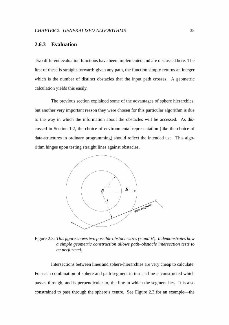
Figure 2.3:This figure shows two possible obstacle sizes (r andR). It demonstrates howa simple geometric construction allows path–obstacle intersection tests tobe performed.
Intersections between lines and sphere-hierarchies are very cheap to calculate.
For each combination of sphere and path segment in turn: a line is constructed which
passes through, and is perpendicular to, the line in which the segment lies. It is also
constrained to pass through the sphere’s centre. See Figure 2.3 for an example—the

CHAPTER 2. GENERALISED ALGORITHMS 36
constructed line is marked as being of lengthl.
If the constructed line intersects the path segment itself (as shown in Figure
2.3), then the distancel from that point to the sphere’s centre is compared against the
radius of the sphere. In this diagram, two different sizes obstacles have been drawn.
Sincel>r then the path segment does not impinge upon the smaller obstacle, but in the
case of the larger circle,l<R, and so it does.
�
Path segment
�
����
Figure 2.4:This figure shows two possible obstacle sizes (r andR). If the perpendicularmeets the extended line (rather than the actual segment) then the distancel′
is used instead.
If the point at which the constructed line intersects the path segment’s line
is not a part of the path segment (this is shown in Figure 2.4), then the distancel is
ignored. Instead, the shorter of the two distances from the sphere’s centre to the path
segment’s two ends is used. Again, the intersection is determined simply by comparing
the distance (in this casel′) against the radius. For this example, the path segment is
clear of the smaller obstacle (l′>r), but not the larger one (l′<R).
Repeating this for all possible combinations of spheres and path segments and
summing up yields the required value. This clearly has a minimum of zero, occurring
CHAPTER 2. GENERALISED ALGORITHMS 37
when all segments of the path are obstacle-free. If such a path is ever found, then the
algorithm may terminate returning this as a complete, valid and collision-free path.
While being relatively simple (both in conception and implementation), this
evaluation strategy does mean that many changes in the path do not give rise to cor-
responding changes in the path’s evaluation (ie. changes in the path can be quite sig-
nificant, but if it still penetrated the same number of obstacles, then it still receives
the same scoring). The solution to this is to treat each intersection not as a boolean
value, but rather as a floating point value indicating how close to the tangential (non-
penetrating) position the line is. Segments that do not penetrate spheres score zero, but
those which do, score a positive value proportional to the extent of the penetration. For
more general representations of obstacles, [16] presents an efficient way to determine
penetration distances. The desired path is one which is obstacle-free, and so scores
zero—again giving a definite target for any minimisation strategy.
It is worthy of note that in both these versions, the geometrical details are care-
fully abstracted away from the optimisation algorithm. The optimisation module deals
with the paths only as black boxes whose interface allows them to be manipulated via
bit-strings. When evaluation of the fitness function is required, then a simpleeval()
routine is called and a hidden implementation containing all the geometric aspects and
calculations is executed. This separation helps keep the algorithm clean, and allows for
the environment’s and path’s representation and the evaluation function to be changed
without effecting the optimisation module.
2.6.4 Selection and cross-over
In each generation, one half of the population is replaced by new paths formed from the
union of two others. Uniform random cross-over is used. To select paths to be replaced,
a biased random choice is made; the probability of a path being chosen for replacement

CHAPTER 2. GENERALISED ALGORITHMS 38
is linearly proportional to its score. No path is replaced twice in one generation. The
selection of parents is also done by biased random selection. The probability of pathpi,
with scoresi, being chosen as a parent is linearly proportional to:maxj(sj) + 1− si.
One of the paths which acts as a parent during a round may be replaced later
in that round, but no new path is a parent in the generation it is created. Each new path
has two distinct parents, neither of which is the one it is replacing.
2.6.5 Mutation
Mutation is performed only on newly generated paths. ApproximatelyMuteRate (∈
[0, 1]) of paths are selected. If a path is selected for mutation, then one randomly chosen
bit in that path’s representation is inverted.
2.7 Completeness, complexity and termination
When using many heuristic algorithms, the problem arises of when to terminate the
algorithm. In this case, the objective functionf ′ has been carefully crafted to have a
particular optimum value: zero. This occurs when, and only when, a path crosses no
obstacles at all (ie. it is completely feasible). So if this value is ever reached, then the
algorithm knows to halt.
The difficulty arises in knowing when to stop after finding no solution. This
might be desirable for three reasons. The first and most straight-forward is that the
original problem might not admit to a solution, in which case an infinite amount of
processing time will still achieve no results. A slightly weaker form of this is that the
original problem does possess a solution, but the value ofm (the number of segments)
chosen was too low for the solution to be represented.

CHAPTER 2. GENERALISED ALGORITHMS 39
Finally, it may be that there is a solution, and that the value ofm is suitable,
but that the solution has still not been found after a long period of time. Usually this is
because the population has prematurely converged and most (if not all) of the population
are clustered about a particular non-global minima.
Detecting any of these three conditions is problematic at best, and distinguish-
ing between them is near impossible.
The second problem—that of settingm too low—can be avoided by always
choosing a high value. However this will slow the calculations which take place at each
generation, and furthermore an overly large value ofm will significantly deteriorate the
rate of convergence (see Table 2.1 and the accompanying text of Section 2.8).
If the algorithm is to be run over environments of a given type, then some
experimentation with examples of these may yield a good set of heuristic conditions.
In general “stagnation” of the genetic algorithm can be detected by noting the diversity
(or lack thereof) in the population. If a large percentage of the population is a short
Hamming distance1 away from each other, then the population has probably converged.
Re-starting the algorithm with a largerm or different initial populationmaysucceed
where the first has failed.
Theoretically, if a feasible solution exists and is representable by a piece-wise
linear path withm segments, then a solutionwill eventually be found. This is due to the
mutation operator. This can be seen as follows: for any given population, consider the
genetic string with the smallest Hamming distance from a correct solution. If this were
to be crossed with another string and the randomly selected uniform cross-over mask
was all 1s, then the chosen string would be reproduced exactly bar mutation. Since
each new string may have one bit flipped, then there is the possibility that this will
reduce the Hamming distance between this string and the correct solution. Repeating1Hamming distanceis a measure of the difference between two binary sequences. If(a1, . . . , ap) and
(b1, . . . , bp) are such sequences, thenHamm(a, b) =∑p
i=0 |ai − bi|.

CHAPTER 2. GENERALISED ALGORITHMS 40
this will give a sequence of strings progressively approaching and eventually reaching
the correct solution. Of course the probabilities at each stage (which are already small)
need to be multiplied, so the overall probability of obtaining a particular solution purely
through the mutation operator is vanishingly slim, but non-zero. This is referred to as
probabilistic completeness.
In the final analysis however, due to the nature of GAs, then there is no way
to know for certain if terminating and restarting is the correct procedure to take. Nor
is there any sure means of determining when to give up on the problem completely.
This then, is the chief disadvantage of employing GAs to solve the motion planning
problem—however it is a problem shared with many heuristic strategies. The author’s
implementation in fact simply stops after a fixed number of generations have been pro-
cessed.
To consider the complexity, a single line–sphere intersection test isO(d),
whered is the dimension of the C-space. To perform an evaluation of one entirem-
segment path againstn spherical obstacles will beO(mnd). A single iteration of the
algorithm (corresponding to one generation) with a population ofP consists of: select-
ing P/2 victims (O(P )), selectingP/2 pairs of parents (O(P )), producingP/2 new
gene strings (each is which isO(dmb) [the length of the string], so makingO(Pdmb)),
and evaluating these new offspring (O(Pmnd)).
The evaluation of the new offspring is the dominant factor, and so each gener-
ation has time complexity
O(Population × NumSegments × NumObstacles × Dimension)
Note that theNumObstacles refers to the number of spheres assuming that no heirachi-
cal decomposition has been used. This was in fact the case in the author’s implementa-
tion; however as discussed in Section 2.6.2, making use of a hierarchical decomposition

CHAPTER 2. GENERALISED ALGORITHMS 41
will (in general) make for significant savings.
In the light of the earlier comments upon termination, then clearly there is no
way of specifying a meaningful worst-case complexity bound for a run of theentire
algortihm.
2.8 Experimental results
A program based upon the above algorithm has been implemented in C++ and tested
on several platforms.
The results tabulated and discussed here for the first part of this section were
all performed in two dimensions for ease of verifying that solutions to the randomly
generated problems did in fact exist. In each case twenty feasible random problems
were generated, each containing ten randomly sized and located circular obstacles. All
the tables below showpairsof numbers. The first of these is the number of times (out of
the twenty runs) that the program failed to find a feasible solution in less thanMaxIter
iterations. The second is an indication of the average amount of work required to obtain
a solution. This average was obtained by taking the total amount of work done in the
twenty trials, and dividing this by the success rate. “Work”, as used here, is defined
to be the number of times a fitness evaluation was performed (ie. the number of times
paths were checked for obstacle intersections).
Table 2.1 shows an interesting point of motion planning. Allowing more de-
grees of freedom in the solution (ie. the number of twists and turns in the path—as
distinct from the dimension of the C-space) than are actually necessary, increases the
work required. Specifically for this algorithm: problems of this type with a given com-
plexity (in this case 10 obstacles) usually have an optimum number of segments (m).
Choosing too few obviously makes the problem insolvable as there is not enough flexi-

CHAPTER 2. GENERALISED ALGORITHMS 42
Table 2.1:Varying number of line segments
Number of Integer method Continuous methodSegments Failures Work Failures Work
3 2 347 3 2334 1 233 2 1685 2 405 4 34210 11 2038 6 659
Population = 50, MaxIter = 25, Mutation = 20%
bility permitted in the solution path for all obstacles to be avoided. On the other hand,
providing too much flexibility makes the task more difficult: now more segments must
be arranged such that they are clear of the obstacles. The data in the table exhibits this
quite clearly, with the optimum for this set of problems being around four. The increase
in work for the higher value of ten is quite marked. The failure rate for ten segments
is the main contributing factor: because the program is frequently terminating before
it has had a chance to converge upon a complete solution, then the amount of work
required on average to find one correct solution increases dramatically.
The other important aspect indicated by this table is the difference that the
choice of evaluation strategies makes. The results in columns two and three were ob-
tained employing the first of the evaluation strategies discussed, where the (integer)
number of obstacle crossings is used. Columns four and five instead used the continu-
ously defined function that indicates theextentof the crossing. This continuous method,
clearly achieves a result after less work. This was expected, as the continuous evaluation
function does give the algorithm more information to work with. In particular, it gives
an indication of whether a small movement in the path (which may still be crossing the
same number of obstacles) is an improvement or not.
The table shows the improvement this extra information provides in all of the
values, and particularly in the more complex problems. It is anticipated that such im-
provements will continue with further increases in the complexity.

CHAPTER 2. GENERALISED ALGORITHMS 43
The results ahown in Table 2.2 and Table 2.3, are produced using the integer
evaluation method.
Table 2.2:Varying the population
Population MaxIter Failures Work6 208 16 502210 125 14 295125 50 6 73240 31 3 41850 25 2 40560 21 3 45770 18 2 42280 15 6 747100 13 7 857150 8 1 594300 4 6 942Mutation = 20%, Segments = 5
Table 2.2 shows the effect of varying the population size on the efficiency and
efficacy of the algorithm. To keep the comparisons fair, then the upper limit on the
amount of work that each algorithm was permitted per run, was kept a constant. That
is, MaxIter × Population = 1250. This allows the failures to be easily compared,
as the maximum number of path evaluations allowed was the same. It is quite evident
from the average work values that too low a population (not allowing sufficient genetic
diversity) or too large a population (preventing sufficient iterations from being done)
results in a significant performance loss. These figures have been plotted and appear in
Figure 2.5. This shows that there is an optimal population for this particular problem at
around 50.
Table 2.3 shows the effect of changing the mutation rate (the percentage of
new paths which are mutated). Small populations (such as used here) tend to be prone
to low genetic diversity, and so suffer a slowing of convergence. In these cases, some
mutation is definitely beneficial. However too high a level of mutation destroys the
good properties of the new paths before they can propagate. In these experiments,

CHAPTER 2. GENERALISED ALGORITHMS 44
Table 2.3:Varying the mutation rate
Mutation Rate Failures Work0% 1 37620% 2 40550% 0 302100% 5 763
Population = 50, MaxIter = 25, Segments = 5
the differences were not marked except for a performance drop in the extreme case of
mutating 100% of the new genetic strings.
The examples shown so far are all two dimensional. To show that this imple-
mentation does in fact support higher dimensions, Figure 2.6 shows the sample output
of the program when run in three dimensions with fifteen randomly placed spherical
obstacles. The program sought to find a path from the lower left hand corner, to the
upper right. A four segment path found by the program that satisfies this is shown.
50 100�
150� 200�
250� 300�
Population size�
0
500
1000
1500
2000
2500
Ave
rag
e w
ork
to
fin
d a
so
luti
on
�
Figure 2.5:Graph showing the effects of trading off number of iterations for populationsize. Data taken from Table 2.2
The previous examples are convenient to generate for testing purposes in sev-
eral dimensions and the resultant figures are easy to comprehend by the reader. However
as evidence that the same algorithm can also be applied successfully to less artificial C-

CHAPTER 2. GENERALISED ALGORITHMS 45
Figure 2.6:Sample output in 3D with fifteen obstacles
spaces, then a more realistic test problem was used. The example chosen is a two-link
revolute planner based upon Figure 12, Chapter 8 of Latombe’s book [65]. The obsta-
cles are fixed, and each of the arms has a joint limit.
To generate the required C-space, the obstacles and the arm itself were first
approximated by a series of circles. Figure 2.7 shows how this was done. To show the
earlier mentioned point that the actual C-space obstacle representation does not effect
the high-level design of the algorithm, then the C-space generated for this example
was a high resolution bitmap. This bitmap is shown in Figure 2.8. It was generated
by calculating the location of each of the circles which constitute the manipulator at
various discrete values ofθ1 andθ2 and testing each of these in turn for intersection
with the circles which comprise the obstacles.

CHAPTER 2. GENERALISED ALGORITHMS 46
Figure 2.7:This figure shows how the obstacles and manipulator arm were approxi-mated by a series of circles.
The genetic algorithm outlined in this chapter was applied to this C-space.
The evaluation function used was simply to count the number of distinct C-space cells
occupied by obstacles which a given path crossed. Figure 2.8 shows the C-space path
found by the algorithm.
The series of images (ordered as numbered) in Figure 2.9 are snapshots of the
workspace at various intervals along the C-space path. These show the manipulator
moving from one region tightly constrained by obstacles to another similar one.
The spurious loop in the C-space path shows that the path found was only
feasible, not optimal. However this could easily be removed in post-processing. Alter-
natively, some kind of optimality (perhaps minimal path length) could be built into the
evaluation function as discussed in Section 2.10.
This example demonstrates that the algorithm is independent of the C-space
representation used (the previous examples used spherical decomposition). As men-
tioned back in Section 1.2, this planner is abstract enough to be implemented with
virtually any representation of the environment.

CHAPTER 2. GENERALISED ALGORITHMS 47
Figure 2.8:The solution path found through the C-space by the GA algorithm
2.9 Parallelisation
With all computationally intensive problems, people’s demands for speed are rarely
satisfied. Even with constant improvements in the speed of consumer-grade hardware,
and slightly slower improvements in high-end hardware, there are still many situations
where faster run times of applications would be appreciated. Motion planning is cer-
tainly not immune to these pressures, and with increasing automation in factories and
smaller more specialised production runs (which need a faster turn-around in planning)
it is becoming ever more important.
A significant speed improvement can be seen in some areas of computer sci-
ence through the use of parallel computers. Thespeed-upof an algorithm due to its
parallelisation is usually defined as the ratio oft1/tp to p, whereti is the time taken
for i processors to complete a particular job. For deterministic algorithms, alinear
speed-up (ie. wheret1/tp =p) is optimal.

CHAPTER 2. GENERALISED ALGORITHMS 48
1 2 3
4 5 6
7 8 9
Figure 2.9:These pictures (left to right, top to bottom) are snapshots of the workspaceas the C-space path in Figure 2.8 is traced out.
Unfortunately, not all algorithms are easily amenable to parallelisation, and
even if they can be parallelised, their speed-up may be significantly less than linear.
Thankfully, genetic algorithms in general, and this application of them in particular, are
amenable to fairly efficient parallelisation. Several authors have researched the general
problem of parallelising GAs [18]. There are several ways of approaching the problem.
The simplest approach is a simple master-slave architecture with the individual
fitness evaluations farmed out to the slaves. The disadvantages are: the processing
bottleneck at the master; high communications requirements; and the wasted processor
time due to unbalanced workloads (this is especially true when the sphere hierarchies
CHAPTER 2. GENERALISED ALGORITHMS 49
are being used as some fitness evaluations may require many more levels of the tree to
be tested against path segments than others). This very fine grained approach would
be suited to a large number of relatively poor processors connected with a specialised
network. However this architecture is no longer prevalent amongst commercial parallel
machines.
Computers with smaller numbers of fast processors are more common. For
these, running independent populations on each processor and swapping a few members
between them at each generation is more efficient (achieving a higher computation to
communications ratio). This means of parallelising comes in two variants. One has
the swapping of selected members between the populations done at each generation.
This is closest in keeping with the original serial version and can work well on a shared
memory architecture, where the communications overhead is low.
The other isasynchronous, the populations only exchange members every few
generations—with the interval perhaps chosen on a dynamic basis. While deviating
somewhat from the original, this further reduces the communications requirements.
Furthermore, it removes all balancing problems as non-blocking sends and receives
can be used. No processor is ever left idle.
It has been argued that this multiple population with asynchronous updates
improves upon the results. While the genetic diversity in each population is smaller
than a combined one would be, the overall diversity will usually be maintained at a
higher level. This is because a temporarily dominant species in one population will not
reproduce and replace all members of the overall population as quickly. That is, delayed
communication is a way of reducing premature convergence. In fact these same authors
go as far as recommending that this “parallel style” GA with the multiple populations
be used even when running in serial on a single-processor machine [80].

CHAPTER 2. GENERALISED ALGORITHMS 50
Results
The asynchronous model was the one chosen by the author for implementation. Sepa-
rately initialised populations evolve on each processor. When a processor has completed
Interval generations, it sends a message containing some of its better individuals to an-
other randomly selected processor. It then checks for any incoming message and adopts
any newly received individuals into its own population.
Donated individuals are randomly chosen, but selection is weighted towards
those with a high fitness. The incoming individuals adopted by a population replace a
set of randomly selected victims. The selection of victims is also weighted—this time
biased towards selecting those with low fitness.
Testing of the author’s parallel implementation was performed on a Silicon
Graphics Cray Origin2000—though the results should be comparable on any modern
shared memory parallel machine.
In the test runs reported here, the population on each processor was 50, and
the number of individuals sent in a message was 5 (ie. 10%). The test problems were
two dimensional square regions with 50 randomly placed obstacles. Mutation was set
at 5% and maximum number of generationsper processorwas 1,000. The program was
requested to find piecewise-continuous paths of ten segments connecting one corner of
the environment to its opposite. Figure 2.10 shows an example of such an environment
along with one of the solution paths which the program found.
Table 2.4 shows the results of running the problem on differing numbers of
processors (p) with varying communications rates. At one extreme (Interval =1), each
processor sent and received selected individuals at each generation. At the opposite ex-
treme (Interval =∞), the populations were entirely independent. For each (Interval , p)
pair, the table shows three figures.

CHAPTER 2. GENERALISED ALGORITHMS 51
Figure 2.10:An example of the problem used in testing the parallel implementation.The solution shown is one generated by the algorithm.
The first is the success rate as a percentage (of the 190 runs). That is, the num-
ber of times the algorithm did find an answer before the maximum number of iterations
was been reached. The second set of figures is an average time required to find a so-
lution. That is, the sum of the wall-clock times divided by the number of successes.
The units of time are such that processing one generation takes one unit of time. The
third value given for each (Interval , p) pair is time1/ptimep
. Sincetime1/p would be the the-
oretical time given a perfect linear speed-up, then this third value gives a measure of
the efficiency of the parallelisation. Note though that with this implementation, linear
speed-up is in fact too pessimistic. This can be seen in this third section of the table
where all but one entry (italicised) is linear or super-linear.
Graph 2.11 presents the timing results of Table 2.4 (note the log-scale on the
x axis). The different lines correspond to running the program with different intervals
between communication. The dashed line shows a calculated linear speed-up based

CHAPTER 2. GENERALISED ALGORITHMS 52
Table 2.4:Varying number of processors and frequency of communications
Success (as %) Time (in steps) per solutionInterval p=1 2 3 4 8 p=1 2 3 4 8
1 60 81 87 93 98 915 386 249 164 835 55 79 89 93 99 1032 374 229 143 7610 53 75 92 96 100 1121 473 204 154 6315 63 82 93 97 98 849 380 214 147 9220 62 75 90 99 100 847 475 233 119 72∞ 56 84 89 97 100 989 361 277 150 79
Efficiency(
time1/ptimep
)Interval p=1 2 3 4 8
1 1.0 1.2 1.6 1.4 1.35 1.0 1.3 1.5 1.8 1.610 1.0 1.1 1.8 1.8 2.215 1.0 1.1 1.3 1.4 1.120 1.0 0.8 1.0 1.7 1.4∞ 1.0 1.3 1.1 1.6 1.5
around the average time for one processor. The graph clearly shows how the actual
data does achieve super-linear performance. This cannot occur in purely deterministic
algorithms—there is always a fixed amount of work to be done. In the literature on
parallel computing are some apparent exceptions to this; but these only occur due to
hardware advantages such as increased amounts of cache memory or better memory-
access coherency. Such advantages may have occurred here, but the “times” given in
table 2.4 are in fact numbers of steps—not strict wall-clock times—and so this is not
responsible for the speed-ups shown.
The reason for super-linear performance in this instance hinges upon the fact
that the parallelised algorithm is not in fact perfectly equivalent to the original serial
version. The differences are the increase in total population with increasingp and the
delayed convergence due to the partial separation of the populations.
Since the populationper processoris a constant 50 in all trials, then the total
population for any given trial is50p. It could be argued that for a “fair” comparison,

CHAPTER 2. GENERALISED ALGORITHMS 53
2 4 8�
1
Number of processors�
0
500
1000
Ave
rag
e ti
me
to f
ind
a s
olu
tio
n
�
Interval=1Interval=5Interval=10Interval=15Interval=20No communicationTheoretical linear
Figure 2.11:Graph showing the average time required to obtain an answer with in-creasing numbers of processors. The different lines correspond to differentdata interchange rates.
the total population should be held equal. Unfortunately what starts off as reasonable
population per processor atp = 1 becomes impractically small with higher values of
p. Too small a population leads to very rapid convergence (as shown in Section 2.8)
preventing proper exploration of the domain. In any case, this author argues that in
almost all practical parallel computers, scaling population along with the processors is
quite reasonable given the small memory footprint of this algorithm. For all general
purpose machines, this algorithm is computation-bound, not memory bound.
This super-linear performance is not uncommon for parallelised non-determin-
istic algorithms. In [19] and [20], the authors parallelise the randomised path-planner
of Barraquand and Latombe [5, 6] that was discussed briefly in Section 2.1. They ef-
fectively run the same program multiple times on the parallel machine in a completely
independant fashion. Due to the non-deterministic nature of the algorithm, each proces-
sor will explore the C-space in a slightly different fashion. As soon as any one processor
has found a solution, the program terminates. They often achieved super-linear perfor-

CHAPTER 2. GENERALISED ALGORITHMS 54
mance with small numbers of processors because the serial algorithm might be delayed
in succeeding due to taking an unfortunate random step at some stage. The multiple
simultaneous searches reduce the likelihood of this delay becoming rate-determining.
For a more general discussion of super-linear speed-ups in GAs, see [88].
It is interesting to consider the effectInterval played in the efficiency of par-
allelising the algorithm here. When there is only one processor (ie.p = 1), then there
is no communication at all, so the value ofInterval is quite irrelevant. It can be seen
from this graph that despite averaging over nearly 200 repetitions, the times forp = 1
(which should theoretically all be the same) do vary by quite a margin. Having noted
this, then care must be taken not to place too much reliance in the relative times for
different Interval values. In fact, considering the values tabulated and these reserva-
tions, then all it is really possible to say is that: any performance impact the choice
of Interval might make is negligible when compared with the variation inherent in the
overall genetic algorithm.
Given this, then settingInterval to be infinite is probably as good a value as
any other and will keep the communications to an absolute minimum (some communi-
cations will still exist, eg. one process signalling to another that it has succeeded).
2.10 Optimal paths
In Section 2.4, the possibility was mentioned of finding optimal paths rather than just
feasible ones. This is not an uncommon desire; usual candidates for optimisation in-
clude: minimum distance travelled, minimum time taken to travel (this applies only to
the dynamic formulation of the problem) and maximising the minimum obstacle clear-
ance. These aims and others can be achieved by simply adding an evaluation of the
path’s optimality to the functionf ′ in some fashion as discussed in Section 2.4. How-

CHAPTER 2. GENERALISED ALGORITHMS 55
ever doing so removes the desirable property of a clear termination condition.
Overall though, this author is of the opinion that this algorithm is better em-
ployed in just finding feasible paths. This maintains the clear termination condition on
success and speeds the finding of a solution. If some kind of optimality properties in
the path are also desired, then these should be deferred until a post-processing step. At
that stage the path can be pruned, smoothed or moved further away from obstacles.
2.11 Dynamic planning
All of the discussion in this chapter to date has focussed on static environments. In fact
this algorithm can easily be modified to support environments with moving obstacles.
Firstly, the dimension (d) of the entire system is increased by one—this new dimen-
sion being the temporal one. The obstacles are extended in the obvious way into this
temporal dimension. This is just the configuration-time space described in Section 1.1.
If the algorithm as described earlier were now to be run on this modified en-
vironment, then an obstacle-free path would be returned. However the resultant plan
would involve backwards travel through time. Removing this problem is by the straight-
forward addition of an additional constraint to the problem. This new term is of the
form:
ct(x) =
0, if slope(x) ≥ 0
|maxmi=0 slope(xi)| , if maxi slope(xi) < 0
whereslope(xi) is the angle that theith segment of the(d + 1) dimensional pathx
makes withd dimensional hyperplane containing all the spatial dimensions.
That is, if the slope is negative (heading backwards in time) then a penalty
term proportional to this transgression is added. Since the optimisation step does not
terminate with an answer untilc(x) = 0, then the optimisation process will force this
CHAPTER 2. GENERALISED ALGORITHMS 56
additive term to zero, ensuring temporal sanity.
A further constraint that is common in dynamic motion problems is that of a
maximum velocity. Without this, many otherwise difficult problems can be solved with
the aid of infinite velocity—something difficult to achieve in practice. This too can be
prevented in a similar manner by adding another term of the same form which gives a
penalty when the slope is too great. Of course depending upon the particular situation,
different velocity constraints might be appropriate for each dimension of the C-space.
The path generated by using this configuration-time space is not directly fea-
sible. The piece-wise linear nature of the path encoding actually requires infinite accel-
eration on the part of the robot at each node. In practice, of course, a post-processing
step would smooth out these abrupt velocity changes.
2.12 Conclusion
This chapter has been devoted to solving the most general kind of motion planning
problem. Due to the complexity of motion planning—especially in the most general
form—exact algorithms are generally too expensive and so heuristics must be used.
One particular heuristic algorithm has been given which shows a number of
advantages over some of its equally general competitors. Given a sufficiently high value
for m, then this algorithm is probabilistically complete. Other GA-based algorithms
existed, but this removes a significant limitation in these.
The planner presented here has a numebr of advantages over other generalised
planners. It is largely independant of C-space representation; only minor changes to
the evaluation function are required. This, and other aspects of the algorithm make
it fairly easy to implement—something that is not true of many planning algorithms.
The fact that it is general enough to support problems of any dimensionality, yet still

CHAPTER 2. GENERALISED ALGORITHMS 57
provide probabalistic completeness is unusual. Finally, it is capable of being efficiently
parallelised on any modern shared or distributed memory machine, as the results in
Section 2.9 show.
General algorithms will work in any situation, and are necessary if either too
little of the problem is known in advance or no specialist planners exist. However given
more information about the environment, a specialised algorithm is almost certain to
win performance-wise. This then, is what the next chapter will be addressing.
Chapter 3
Specialised environments
The previous chapter showed how a general motion planning algorithm could be de-
signed to successfully solve planning problems involving virtually any environment
and robot. Section 2.7 proved that given a sufficiently large value form (the number
of segments in the path) the algorithm presented was probabilistically complete. How-
ever it was explained that to reach this “guaranteed” solution, an impractical amount of
time may be required. This potentially extended runtime is of course a function of the
C-space through which the planner must find a route.
This situation is certainly not unique to the GA planner described. Most plan-
ners have at least one kind of C-space in which they are known to perform poorly. Some
of these pathological examples are very specific to the particular problem, but some are
relatively general and are particularly troublesome for many different planners.
Given sufficient information about the environment in advance, then a planner
may be chosen which is expected to perform well in that situation. This chapter con-
siders one such type of problem environment: one where the C-space contains narrow
gaps and passages.
The reason why these gaps and passages cause problems for so many planners

CHAPTER 3. SPECIALISED ENVIRONMENTS 59
is considered, and a survey is made of those few planners which do successfully cope
with them. As a particular example, an algorithm designed by the author will be exam-
ined. This algorithm is a specialised one: while not perhaps as fast as others in general,
it does support planning in C-spaces with narrow passages in a very efficient manner.
Narrow passages and gaps in C-spaces can arise from a number of different
situations in the workspace. Probably the most common occur when motion in the
workspace is tightly confined. Simple to visualise cases of this are: a vehicle forced to
move down a corridor only just wider than the vehicle itself; or a long thin manipulator
having to reach through a gap in a wall to adjust something on the other side.
An extreme case occurs in assembly problems (where a robot manipulator
must assemble some device from that device’s constituent parts). When an axle or
shaft must be inserted, the “play” of the shaft (how much freedom it has to deviate from
an arbitrary correct path) is minimal. Now to be fair, this situation is probably best
not planned using a normal planner, but instead controlled in real-time with a force-
feedback loop and sensor, however it does show how the situation can arise.
3.1 Planners that perform poorly
The first two chapters of this thesis discussed a number of different existing planners,
unfortunately the majority of these all perform poorly on environments with narrow pas-
sages. A number of these algorithms are touched on again here with a brief explanation
of why they succumb to this particular family of environments.
A large number of planners use a cell-based decomposition of the environment.
As mentioned in Section 2.1, these suffer from the problem of resolution completeness.
Narrow gaps and passages—especially those whose edges are not aligned with the axes
used in the decomposition—can easily escape being correctly represented in the cell-

CHAPTER 3. SPECIALISED ENVIRONMENTS 60
based representation. A particular case of this was shown in Figure 2.2. Knowing just
how fine to make the discretisation is no trivial task, and the small C-space passage
which is lost through this representation may be an essential part of the solution.
Potential-based planners are sometimes implemented as cell-based methods,
however even if not, they are almost certain to have a locally high potential in the C-
space gap or passage. This is an unavoidable artifact of the region being closely pressed
by the enclosing obstacles. The potential field is a function of obstacle proximity and
distance to the finish. Over the short distance from just outside the “mouth” of the pas-
sage to inside it, the change in potential due to distance from the finish will be small in
comparison with the increase due to the obstacle proximity. This means that a strictly
descent-based planner will never try this passage as doing so requires a temporary in-
crease in potential.
Barraquand and Latombe’s variation [5, 6] upon this uses a random walk to
escape local minima. This may be successful in the case of a narrow gap in a C-space
wall as the walk could well make the few potential-increasing steps required to move
to a new lower potential on the far side. However this is far less likely in the case of
a more extended region of high potential, as occurs in a narrow passage. In this case
the number of potential-increasing steps required becomes significantly higher, so the
likelihood decreases.
The PRM method described in Section 2.1 is extremely effective in rapidly
exploring open regions of C-space. However it too suffers when the C-space includes
a narrow but critical passage or gap. The PRM’s representation of the connectivity of
free-space is dependent upon the randomly selected points. In the confined regions of a
narrow passage, only a small amount of space is actually feasible, and so the likely-hood
of a valid point being chosen in that region is relatively small. A full implementation
of the PRM is not limited to just selecting uniform random points. At later stages in
its execution, the algorithm will attempt to bias the selection of points towards regions

CHAPTER 3. SPECIALISED ENVIRONMENTS 61
with poor connectivity. This will help in the case of a passage—though at the cost of
testing many invalid points from the surrounding area. However it will be less effective
at helping with narrow gaps in a wall as the general connectivity of the area will be
reasonable (points near the wall will have normal connectivity with other points on the
same side).
Being probabilistically complete, the PRM will succeed—but quite possibly
only very slowly. The PRM’s poor performance in narrow passages is a known prob-
lem and attempts are being made to redress this [45]. Section 4.6.3 discusses a partic-
ular example of an environment of narrow passages in which the PRM proves slow to
execute.
In [13], Brooks usesgeneralised conesas a way of representing (some of)
the free portions of the workspace (as distinct from C-space). A generalised cone is a
region of space swept out by moving a (possibly varying) cross-section along an axis. A
graph is formed with edges corresponding to the cones’ axes and nodes corresponding
to where these axes cross. The final solution path is generated by searching through this
graph, testing for rotational clearance at each node. These axes make for very practical
routes for a robot to follow as (in general) they will be well removed from the obstacles.
This is a reasonably efficient algorithm that produces paths with good practical
clearance. Due to its chosen representation of the free-space (being based directly on
obstacle geometry), it might be hoped that it is immune to the problems of narrow gaps
and passages. However in practice, Brooks noted that it does not perform well in tightly
constrained environments—not all portions of free-space are covered by the cones. In
addition, it only supports two dimensional work-spaces, and is known to be restrictive
in its ability to handle turns. This latter limitation occurs because all turns are made
at axes intersections; the rest of the route is traversed with the orientation of the robot
matching that of the respective axes.

CHAPTER 3. SPECIALISED ENVIRONMENTS 62
3.2 Planners that succeed
While the previous section showed that many existing planners do perform poorly in the
presence of narrow passages and gaps, a couple of existing planners are more success-
ful. The common characteristic shared by both is that they perform their calculations
directly on the obstacle geometry itself; not on some approximating representation that
does not well capture the critical narrow spaces and passages.
The Voronoi method mentioned back in Section 1.2 works directly with the
C-space obstacle geometry to find sets of points that are equidistant from two or more
obstacles. This ensures that even a narrow gap or passage will be suitably represented
internally, and so not overlooked. Minor variations upon this exist which use non-
Euclidean distance metrics. These work well in two dimensions. Unfortunately it is
rarely used in higher dimensions as it is not obvious what to select for the features [46].
Canny’s silhouette method [17] generalises the Voronoi method to higher di-
mensions. It works by recursively projecting curves through the environment into lower
dimensional spaces. However it is mostly used in theoretical algorithms for analysing
complexity, rather than developing practical algorithms [46].
Another planner that works directly with the obstacle geometry is thevisibility
graph method(used in [53, 54] amongst others). This is another roadmap planner.
It is somewhat a brute-force sounding algorithm, but it does guarantee completeness
and in two dimensions is optimal in path length. All C-space obstacles are taken to
be polyhedra (convex or concave). A graph is constructed. The nodes of this graph
correspond to a set of points in the C-space consisting of the given start and end points
and each of the obstacles’ vertices. For each possible pair of points in this set, a test is
made to see if the straight line segment connecting them in C-space passes through any
obstacles. If such a line segment is found to be collision-free, then an edge is added to
the graph connecting the two corresponding nodes. Once this sub-set of the complete

CHAPTER 3. SPECIALISED ENVIRONMENTS 63
graph is formed, a graph search gives the route the robot should take.
This algorithmdoeswork effectively, even when the C-space obstacles have
narrow gaps or passages, as again, it works directly with the underlying C-space obsta-
cle geometry.
The above is a way of visualising how the method works—in practice, the
brute-force approach is best avoided for reasons of efficiency. In the case of two di-
mensional problems, the construction of the visibility graph (so called because edges in
the graph correspond to points that can “see” each other with no intervening obstacles)
can be solved using a specialised approach such as in [2] or [95]. These are far more
efficient (O(n2), wheren is the number of vertices) and work by performing a radial
sweep about each point in turn. Unfortunately these efficient methods cannot easily be
extended to higher dimensions, and so the visibility graph method is rarely employed
in higher dimensions.
The final existing method that will be discussed in this chapter is that of Tomi-
naga and Bavarian in [92]. This too works directly with the obstacles’ geometry, though
it is a good deal more constrained in the problems it solves than the previously men-
tioned ones—it works only with circular obstacles in two dimensional environments.
Their method is toembedthese two dimensions in a three dimensional space. Thex-y
plane of the original C-space environment corresponds to thez = 0 plane of the new
space; the circular obstacles of the original become hemispheres. The centres of these
new hemispheres correspond to those of the original obstacles, ie. if the original circle
has a centre of(x, y) and radiusr, then the hemisphere has centre(x, y, 0) and radiusr.
A solution connecting the start and finish points is easily found in this new
space—it goes “over” all the hemispherical obstacles. The method employs a function
which takes as a parameter the current path and returns a value based upon the path’s
proximity to obstacles, and its location in thez-dimension. The algorithm uses a nu-

CHAPTER 3. SPECIALISED ENVIRONMENTS 64
merical optimisation technique (that of Lagrangian multipliers) to modify the path so as
to minimise the function’s value. By including the path’sz component additively in the
function, then the minimisation gradually forces the path to lie in thez = 0 plane. At
this stage the path (stripped of its third ordinate) is a solution to the original problem.
Since it works directly with the obstacle’s geometry, then there is no way that
a critical narrow gap between obstacles (a narrow passage between pairs of circles can
not really occur) can be “missed”. So within the rather restricted set of problems it
supports, this is quite an effective algorithm.
3.3 Overview of a new algorithm
The remainder of this chapter is dedicated to explaining a novel heuristic algorithm
which: successfully navigates through narrow passages; works in any dimension; and
has strict upper bounds on time complexity.
The C-space obstacles supported in this algorithm are fairly general: concave
and convex polyhedral obstacles are supported. Concave obstacles are first decomposed
into overlapping convex polyhedrons—which is what the algorithm directly supports.
As with many algorithms, curved obstacles must be approximated by bounding polyhe-
drons. The path returned by the algorithm between the given start and finish points is
piece-wise linear.
The originald dimensional C-space (C) is extended to an(d + 1) dimensional
one (C ′). Throughout this chapter, this additional dimension will be referred to as thee
(embedding) dimension. The firstd dimensions ofC ′ are identical to those ofC. The
d dimensional hyper-planee = 0 within C ′ is exactlyC. The idea is to construct a set
of (d + 1) dimensional obstacles inC ′ each corresponding to one obstacle inC. These
new obstacles protrude into theeth dimension in the positive sense and taper off with

CHAPTER 3. SPECIALISED ENVIRONMENTS 65
increasinge to an apex with finite height. The cross-section of eachC ′ obstacles is
similar to its corresponding original obstacle in all planese=c wherec is a constant.
Figure 3.1 illustrates this for the cased = 2. The original two dimensional
obstacles were a triangle and three quadrilaterals. These have been extended ine (in
this case the third dimension) to form three dimensional obstacles. The exact choice of
heights and the additional lines will be explained later. This is a very simple problem
for which other planners may well perform better, but it is one that lends itself to easy
depiction, and so will be referred to throughout this chapter.
Figure 3.1:A trivial two dimensional example for visualisation.
The proposed algorithm is given the desired starting and finishing points in C-
space:S andF . Two new points,S ′ andF ′, are constructed inC ′. These are chosen so
that when they are projected upon thee=0 plane, they becomeS andF (respectively).
The value of theeth ordinate in these two points is the same, and is chosen to be greater
than the maximaleth ordinate of all the newC ′ obstacles. In Figure 3.1,S andF are at
the base of the two vertical “poles”,S ′ andF ′ are at the tops.
A trivial obstacle-free path throughC ′ (as distinct from through the original

CHAPTER 3. SPECIALISED ENVIRONMENTS 66
spaceC) connectingS ′ to F ′ is simply a straight line between them since this is known
to be “above” all the obstacles. The goal of the algorithm is to progressively modify this
initial trivial solution in a way that is monotonically decreasing ine. At all times care
is taken to ensure that the path never enters any of the new obstacles. The entire path
is always kept in a single moving planee = c. When the path finally reaches the point
at which it is entirely contained within thee = 0 plane, then striping off the(d + 1)th
ordinate of the path’s description yields a complete, feasible solution to the originald
dimensional problem.
The next section details how these new obstacles are constructed. Section
3.5 discusses how the descending path is represented, and distorted by the obstacles
it hits. Section 3.6 comments on the completeness and correctness of the algorithm.
Finally, Section 3.7 reports on how an implementation by the author performs on some
interesting test problems.
3.4 Constructing the new space
Rather than storing the new obstacles as solid(d+1) dimensional objects, the algorithm
instead uses wire-frame outlines. Each of the C-space obstaclesO(i) can be exactly
represented as a set of points—those that form its convex hull (as earlier stated, all non-
convex obstacles have been decomposed into overlapping convex ones). The obstacles
in C ′ consist of a series of line segments. These segments come in three different types:
primary, multi-obstacle and boundary. The construction of each of these, along with
motivation, will be explained in Sections 3.4.1, 3.4.2 and 3.4.3. Together they form the
newC ′.

CHAPTER 3. SPECIALISED ENVIRONMENTS 67
3.4.1 The primary obstacle lines
Each primary obstacle line inC ′ corresponds to one of the vertices in the originalC
obstacles. These lines are formed by considering each of the obstacles inC in turn. For
O(i), theith obstacle ofC:
• For each of themi verticesO(i)j , create a new pointtj =
{O
(i)j , 0
}(ie. the same
point in thee=0 plane).
• Calculate the centroid of the original points and call ittc. This is easily done:
tc =
∑mij=1 O
(i)j
mi
• Promotetc to (d + 1) dimensions:tc ={tc, 1}. This will henceforth referred to as
theApexof theC ′ obstacle.
• Now themi lines comprising theith C ′ obstacle are those connecting(tj, tc) for
eachtj.
The resulting collection of lines are part of a(d + 1) dimensional polyhedron resting
on a base which is the original obstacle. In the example in Figure 3.1, there are three
primary obstacle lines for the triangle obstacle, and four each for the others.
3.4.2 Overlapping obstacles
One of the problems this algorithm faces is that obstacles may overlap. If this were to
happen and the initial choice of path were unfortunate, then the descending path might
well become “trapped”. That is, it would reach a point where it was at the base of
the valley between two overlapping obstacles, but still not ate = 0. Figure 3.2 shows
an example of this. Of course this can be detected, and some kind of back-tracking
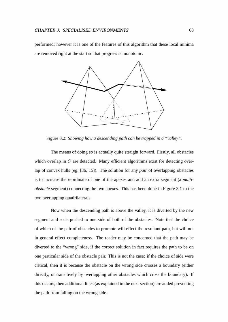
CHAPTER 3. SPECIALISED ENVIRONMENTS 68
performed; however it is one of the features of this algorithm that these local minima
are removed right at the start so that progress is monotonic.
Figure 3.2:Showing how a descending path can be trapped in a “valley”.
The means of doing so is actually quite straight forward. Firstly, all obstacles
which overlap inC are detected. Many efficient algorithms exist for detecting over-
lap of convex hulls (eg. [36, 15]). The solution for anypair of overlapping obstacles
is to increase thee-ordinate of one of the apexes and add an extra segment (amulti-
obstaclesegment) connecting the two apexes. This has been done in Figure 3.1 to the
two overlapping quadrilaterals.
Now when the descending path is above the valley, it is diverted by the new
segment and so is pushed to one side of both of the obstacles. Note that the choice
of which of the pair of obstacles to promote will effect the resultant path, but will not
in general effect completeness. The reader may be concerned that the path may be
diverted to the “wrong” side, if the correct solution in fact requires the path to be on
one particular side of the obstacle pair. This is not the case: if the choice of side were
critical, then it is because the obstacle on the wrong side crosses a boundary (either
directly, or transitively by overlapping other obstacles which cross the boundary). If
this occurs, then additional lines (as explained in the next section) are added preventing
the path from falling on the wrong side.

CHAPTER 3. SPECIALISED ENVIRONMENTS 69
On some occasions, three or more obstacles will overlap (asuper-group). This
does not require that all three share a common point, but rather that they satisfy the
weaker condition that obstaclesA andB overlap and so too doB andC. In these
situations, only one of the apexes is promoted in thee dimension (this is thesuper-apex).
A multi-obstacle segment is added connecting each the the other apexes to the newly
promoted one. Once again, the selection of which apex to promote is arbitrary, though
the final resultant quality path may be effected by the choice. Given this potential
effect, then theoretically the choice could be made so as to optimise the path (according
to some metric), but making this choice would then become very expensive.
3.4.3 Boundary crossings
The other situation which must be addressed is the case of one of the obstacles crossing
the boundary ofC. If this was not dealt with, then there is the possibility of the path
sliding off one side of the obstacle and falling outside theC space—thus becoming
infeasible. This can be resolved in a manner similar to overlapping obstacles.
For each boundary ofC that an obstacle crosses, a corresponding point is cho-
sen on the boundary ofC ′. This point is given ane-ordinate greater than any than any
of the apexes or super-apexes. A line-segment connecting this point to the apex of the
offending obstacle is added. Now, if the path descends on the boundary-crossing side of
the obstacle, it will be diverted away in a similar manner to the multi-obstacle segments.
In the case of the obstacle being part of a super-group, then the line is added,
not to the apex of the offending obstacle, but to the associated super-apex.

CHAPTER 3. SPECIALISED ENVIRONMENTS 70
3.5 Calculating the path’s descent
The path returned by the algorithm is piecewise linear and connects the given start
and finish pointsS andF . The path is completely represented by storing the current
coordinates of all the nodes (a node is where two path segments join) on the path. The
number of segments in the path at any given stage during the calculations varies, but is
initially one. The height of each of the nodes (thee ordinate of each) is the same across
the entire path as it descends—that is, the path at any instant is completely contained
within the planee=c.
The initial path is just the single line-segment connectingS ′ andF ′. The first
d ordinates of these two nodes remain fixed throughout the entire procedure. The plane
containing the path descends (ie.e = ci whereci < ci−1) until the path first encounters
an obstacle segment (or potentially several simultaneously). New nodes are added to
the path where the encounter took place, and the path’s plane descends again. Any
node which lies on one of the obstacle segments, is constrained to continue to lie on
that segment (ie. it may not cross through the segment). The height at which the next
encounter between any section of the path and the obstacle segments occurs, is where
the path again pauses. A new node is inserted for each encounter (more than one if
several occur in the samee = ci plane). So each encounter results in a new node, and
the splitting of one path segment into two.
If a node is following a multi-obstacle or boundary-crossing segment then it
will eventually reach the end of this (since all such segments stop at or before the height
of an ordinary apex). However the obstacle segments are such that one or more new ob-
stacle segments will be starting there, and so the incoming node will always be replaced
by one or more of these.
Finding the point of intersection is a matter of solving a simple system of
equations. Each path segment is treated independently and the highest encounter found

CHAPTER 3. SPECIALISED ENVIRONMENTS 71
�
�
�
�
�
��
�
�
path segment
Descending
Figure 3.3:ef is a descending path segment withe andf constrained to remain onbaanddc respecively.xy is the path the segment is about to intersect.
across all sections is used. The equation of a path segment as it descends along two
obstacle segments may be parameterised byh, the height. A line intersection calcula-
tion is performed between the parameterised equation of the segment and each nearby
obstacle line as is explained.
Figure 3.3 shows the situation of one segment of the path,ef descending. The
nodee is constrained to lie on the obstacles segmentba. Likewisef is constrained to lie
on obstacle segmentdc. These two segments have been normalised so thatb andd have
the same height in the embedding dimension. Likewisea andc are at the same height.
Therefore,e(h)=a + (b− a)h andf(h)=c + (d− c)h. The linexy is another obstacle
line which the path segment is approaching. The eventual point of intersection (which
is to be found) will beg which can be expressed in two ways:g(s)=x + (y − x)s and
g(r) = e + (f − e)r. By combining all four of these equations a system of equations
parameterised byh, s andr is given. Since the dimension is at least 3, then this system
can be solved and sog found. After some checks (eg.g does not lie below the plane

CHAPTER 3. SPECIALISED ENVIRONMENTS 72
e=0) then this value becomes a candidate for the next point of intersection.
3.6 Completeness, correctness, etc.
Algorithms are usually evaluated on five criteria: correctness (will it ever report an
incorrect solution); termination (will it always finish); completeness (will it always
give an answer if it finishes); efficiency (how fast does it find an answer); and quality
(how optimal is the solution, if there is more than one possible answer). Each of these
is discussed in turn below.
3.6.1 Termination
Proof of eventual termination is straight-forward. The descending path’s plane starts at
a given finite height higher than any of the obstacle segments. At each stepi, the heights
of all sections of the path arehi. The seriesh0, h1, . . . is monotonically decreasing in
uneven but finite steps. Ifhi ever reaches zero, then the algorithm terminates with
an answer. An obstacle segment encountered by one descending path section cannot
interact with any of the other path segments. So the maximum number of possible
interactions isN (the number of obstacle segments). Since each step (a movement of
the path-plane fromhi to hi+1) corresponds to one or more such encounters, then the
total number of steps cannot exceedN .
One of two things must occur: eitherhi = 0 for somei≤N (ie. success); or
else at some stepi (i≤N ) no way is found to continue the monotonic series. In this
later case, the algorithm has failed to find a solution path and so aborts. In either case
termination is guaranteed withinN steps.

CHAPTER 3. SPECIALISED ENVIRONMENTS 73
3.6.2 Correctness
If the algorithm does terminate with an answer, then that answer will be a correct one—
this can be shown by induction. Consider the finite number of intermediate stages where
the path’s plane is ate = h0, h1, . . . Each stage can be considered correct if the path
contained in thed dimensional planee=hi does not pass into any of the obstacles (the
obstacles are simplyd dimensional cross-sections of the(d+1) dimensional obstacles).
Certainly this is true ath0, as this value is chosen to be greater than than any of
the obstacles. Given that it is true athi, then it can be shown to be true athi+1: this can
be done by considering the way the path moves as it descends. At stepi, all segments
of the path are either in contact with the edge of one of the obstacles, or are completely
outside of them (free segments).
As the path descends, at the first interaction between any of the free segments
and an obstacle, the descent stops (ate=hi+1). This segment (or possibly several simul-
taneously) does not enter the obstacle—it stops short of doing so. Any other segments
which were outside obstacles at theith step are still outside (to be otherwise, they must
have intersected one of the obstacles on entry, but this is the first such interaction since
e=hi).
As per the algorithm, those path segments which were already in contact one
of the obstacles in stepi are carefully constrained (see Section 3.5) to remain on the
edge of the obstacle (ie. not enter it). Thus by stepi + 1, the condition that the path
does not enter any of the obstacles is still satisfied.
By induction it can be seen that the path never enters any of the obstacles at any
step of the sequence. So at the final stepe=hf (=0) this must still be true. In Section
3.3 the planee = 0 in C ′ was defined to be equivalent toC (the original C-space), so
the path at stagehf must lie outside (or just on) all of the original obstacles. So the

CHAPTER 3. SPECIALISED ENVIRONMENTS 74
algorithm is proved correct.
3.6.3 Quality of path
The algorithm is deterministic except for the selection of which apexes to promote.
Such selection may effect which family of paths the algorithm will find. It is worthy of
note that the path the algorithm returns will have many tangential contacts with obsta-
cles. Ford=2, this is actually optimal in distance for the family of paths it represents;
however it does place rather strong requirements upon the robot’s control capabilities.
This is not of great concern though, as a number of algorithms exist which can easily
post-process the path to a smoother and less positionally demanding curve in the same
family. It is not uncommon for various planners to perform such post-processing, eg.
[77].
3.6.4 Efficiency of execution
For a naive implementation, the worst case involves every obstacle segment interacting
with descending path once. Each intersection that occurs results from testing each of
the path sections against each of the obstacle segments. Initially there is only one
path section; this could have up toN tests performed upon it (whereN is the number
of obstacle segments). Then each of the two resultant path sections would be tested
against theN obstacle segments. FinallyN − 1 path sections would be tested against
N segments. So total number intersection tests would be∑N
i=1(iN) = O(N3). This is
not directly dependant upon the dimensionality of the problem,d.
To perform the intersection test requires solving the set of equations described
in Section 3.5. It should be noted that this isnot solving for the full coordinates of the
pointg (see Figure 3.3)—that would be anO(d) operation. Rather this is simply finding

CHAPTER 3. SPECIALISED ENVIRONMENTS 75
the height at which the intersection occurs (to determine which intersection happened
first). This means simply solving the equations in Section 3.5 forh, anO(1) operation.
So the intersection tests give a cost ofO(N3) × O(1) = O(N3). In addition to the
tests, at each of theO(N) intersections (once the height of the intersection has been
determined) the coordinates ofO(N) nodes need updating—each anO(d) operation.
This brings the total cost toO(N3 + N2d).
Now since the number of obstacle segments,N , is O(V ) whereV is the num-
ber of obstacle vertices, then the total worst-case complexity isO(V 3 + V 2d). It may
seem suprising that theV 3 term is not a function ofd, however it is implicitly as
V = O(nd) wheren is the number of obstacles—this is because any obstacle can
be decomposed into simplexes each of which containd+1 vertices. That is, the overall
complexity isO(n3d3 + n2d3) = O(n3d3).
Also, the author speculates that by selectively choosing which obstacle seg-
ments to test each path section against at each stage, theO(V 3) might be reduced to
O(V 2 log V ). This could probably be acheived by maintaining a list for each path seg-
ment of which obstacle segments were possible candidates for a collision. At the cost
of some bookkeeping, the number of intersection tests would be reduced.
This compares favourably with the visibility-graph method (described in Sec-
tion 3.2) ford > 2. In it, the complete graph formed containsO(V 2) edges, each of
which corresponds to testing a line for intersection against every obstacle.
In practice, tests are not done between lines and polyhedra, but between lines
and facets. Each facet is defined by a series of half-planes. Testing if a line passes
through a half-plane is anO(d) operation. The number of sides to a facet isO(d), and
the number of facets in an obstacle isO(d). So to test one line against one obstacle is
O(d3); testing one line against alln obstacles isO(nd3).
This O(nd3) operation must be completedO(V 2) = O(n2d2) times for the

CHAPTER 3. SPECIALISED ENVIRONMENTS 76
complete visibility-graph to be generated. This gives a total complexity ofO(n3d5).
3.6.5 Completeness
The algorithm as described is not complete. There do exist a small number of combina-
tions of environments and start/finish locations for which a solution will not be found.
However if the algorithm ever does fail in this way, it can detect the fact (and so avoid
returning a false-negative). Furthermore it appears that is may be possible to solve these
problem situations.
1
2
2
1
Figure 3.4:An environment containing two interlocking pairs of overlapping obstacles.This can sometimes cause problems for the algorithm described here.
The problem occurs when one set of overlapping obstacles is in close proxim-
ity with either another set of overlapping obstacles or a boundary crossing obstacle. In
these situations, it is possible for the extra obstacle lines to interlock and prevent the
path from completing its descent (if the path happens to be diverted to this region of the
environment).
Figure 3.4 shows such a situation. There are two pairs of overlapping obstacles.
The numbers indicate the heights of the four apexes and the heavy lines (with arrows
pointing “up” the slope) are the multi-obstacle lines.

CHAPTER 3. SPECIALISED ENVIRONMENTS 77
Although it has not been fully investigated, a solution appears possible. The
trick is to ensure that none of the multi-obstacle lines are outside of the obstacles when
projected onto thee=0 plane. For two overlapping obstacles this is simple: rather than
having two apexes and a connecting line (which might pass through free space when
projected ontoe=0, as it does in Figure 3.4), instead the two apexes could be merged
into one that sits over the point of overlap. Being convex obstacles, then all the points
in both obstacles will be able to be joined to this apex without crossing free space.
For situations where more than two obstacles overlap each other, then the sit-
uation becomes more complex. All existing apexes would be removed and a new one
would have to be formed at every point of overlap. Obstacle edges would be drawn
from the obstacle vertices to any one of the apexes associated with that obstacle (each
obstacle will have one apex for each obstacle it intersects with). All the apexes asso-
ciated with a single obstacle should be joined (directly or transitively) by apex-to-apex
multi-obstacle lines.
The one remaining concern is how to assign heights to each apex. One of the
apexes in the super-group must be selected (possibly arbitrarily) as the highest. Each
apex connected directly to it must be a little lower, and each apex joined to them must
be lower still (and so on). This is effectively a breadth-first search of a graph (where
the apexes are nodes) with strictly monotonically decreasing heights being assigned
to apexes as the search progresses. If one of the obstacles crosses a boundary, then
the boundary-crossing line must go to one of its apexes which must be selected as the
highest of the super-group. In the case of cycles in this graph, an apex is not reassigned
a height if reached again.

CHAPTER 3. SPECIALISED ENVIRONMENTS 78
3.7 Implementation and results
The author has implemented the algorithm described in this chapter. The obstacle in-
tersection routine (used to identify super-groups) used Cameron’s enhanced GJK algo-
rithm [15]—his C routine for this was used with kind permission. Tests have shown the
planner’s implementation to work correctly as expected. Four examples are discussed
in this section.
The first example (shown in Figure 3.1) is uninteresting, but useful for illus-
trative purposes to clarify for the reader how the algorithm works. The original C-space
is two dimensional and has four obstacles (a triangle and three quadrilaterals). TheC ′
for this environment is three dimensional. The two overlapping quadrilaterals have a
multi-obstacle line added connecting their apexes. The path began by connecting the
tops of the two vertical “poles” and gradually descended, deforming as it progressed to
avoid the obstacles. The dashed line shows the final result.
The two dimensional situation is very easy to understand since all three dimen-
sions (the two original plus one embedding dimension) can be easily depicted and vi-
sualised. To assist the reader in conceptually seeing how the algorithm works in higher
dimensions another simple environment is provided, this time in three dimensions. The
environment contains only two obstacles: a cube and a tetrahedron. Figure 3.5 shows
this environment. The reader should be clear in their mind that this three dimensional
image is in fact a three dimensional C-space—whereas the three dimensional image in
Figure 3.1 was of atwo dimensional C-space embedded in a third (ie. Figure 3.5 does
notshow the embedding dimension).
The first (top) diagram in Figure 3.5 shows the environment along with the
algorithm’s initial path, projected into thee = 0 space. Recall that the initial path
is simply the straight line connecting the start and finish, but lying “above” (in thee
dimension) all the obstacles. At this point the path is clear of all obstacles in the four

CHAPTER 3. SPECIALISED ENVIRONMENTS 79
Finish
Start
Finish
Start
Finish
StartFinish
Start
Figure 3.5:Successive snapshots of a three dimensional projection (ontoe = 0) of thefour dimensional embedded space.

CHAPTER 3. SPECIALISED ENVIRONMENTS 80
dimensional space even though it passes through both obstacles when projected onto
e=0.
There are (invisible) obstacle segments going from each vertex of the original
obstacles to the four dimensional apexes. The path descends until it intersects with one
of these—this is roughly (though not quite) the same as “growing” the three dimensional
obstacles from points, and diverting the path as the growing obstacles reach it. The first
of the obstacle segments to be reached is the one connecting the uppermost point on the
tetrahedron to its apex. The path breaks into two here, then continues to descend in the
e dimension until another obstacle segment is reached. Where the path halts this second
time is shown in the second diagram from the top. Now the lower-left segment of the
path splits too and all three segments continue their descent.
The third diagram from the top shows the situation a little later. The algorithm
does not actually stop here since there are no more intersections, but this shows the dif-
ferent directions that the two internal nodes are now progressing in. The final diagram
shows the state when the algorithm is complete. Both nodes escape from the projection
of the obstacles at the same time and so the final path is the one shown, with tangential
brushes against one corner of each obstacle.
A more interesting example shows off one of the features of this algorithm:
its ability to navigate through environments with narrow passages and gaps. Figure
3.6 shows another two dimensional C-space. The path to get from the top-left to the
bottom-right requires maneuvering through three narrow gaps in walls separating large
expanses of valid regions.
Most planners would fare very badly with this problem. Resolution-complete
planners can easily be defeated or rendered too memory-intensive by reducing the gap
size (which has no effect on the planner put forward by this paper). Many graph-based
planners (eg. PRM or the GA based planner put forward in the previous chapter) are

CHAPTER 3. SPECIALISED ENVIRONMENTS 81
Figure 3.6:For most planners this kind of C-space would be very difficult to plan in.
probabilistically-complete, and so will eventually solve this problem but require ex-
tended amounts of time before they successfully found a path fragment through each
gap. The planner put forward here however solved the problem (as shown) in less than
a second on a slow PC.
In Section 2.8 a practical problem was outlined to test the GA based planner
of the previous chapter. The same problem of the two link revolute manipulator is
addressed again as some evidence of the practical use of this chapter’s algorithm.
Figure 3.7 again shows the C-space corresponding to this arm and environ-
ment. The shaded regions are the C-space obstacles; these have been decomposed into
convex sections (delimited by black lines) for use by the planner. This was done by
hand, but in practice would be automated. Care must be taken not to artificially de-
stroy any narrow passages by employing approximate bounding polygons. Note the
long narrow regions of feasible space which would pose problems for many popular
planners.

CHAPTER 3. SPECIALISED ENVIRONMENTS 82
Figure 3.7:The C-space for the two-link arm.
The algorithm of this chapter was applied to the problem: its C-space solu-
tion is shown in Figure 3.7. Figure 3.8 shows a series of snapshots of the workspace
at various intervals along this C-space path. They show the manipulator moving from
one region tightly constrained by obstacles to another similarly constrained region. The
middle frames show the manipulator maintaining tangential contact with the obstacles.
This corresponds to the C-space path being co-linear with several of the C-space obsta-
cles’ edges, as was discussed in Section 3.6.3.
3.8 Conclusion
It has been shown in this chapter that more specialised planners can be developed which
work effectively with particular kinds of C-spaces. It may be that the C-space has some
feature that can be taken advantage of (eg. all obstacles are convex and sparse). Another

CHAPTER 3. SPECIALISED ENVIRONMENTS 83
1 2 3
4 5 6
Figure 3.8:These are snapshots of the workspace as the C-space path in Figure 3.7 isexecuted (order is as numbered).
possibility is that there may be features that would significantly slow a more generalised
algorithm. A particular case for which this was explored in some detail was when the
C-space contains narrow gaps and passages. The algorithm developed to solve such
problems has been shown to be effective (where other more general algorithms would
have failed) on several examples: both contrived problems (designed to be particularly
awkward) and on a more realistic one.

Chapter 4
Specialised modes of locomotion
The previous chapter showed how an algorithm can be designed to efficiently support
C-spaces containing particular features. However it was still generic in the kind of robot
being planned for. This chapter introduces yet another class of heuristic algorithms; this
time for a specialised class of robots: vehicles with legs.
The two previous chapters have been for generalised devices and would apply
equally well for both manipulator arms or vehicles. This chapter deals exclusively
with vehicles and legged locomotion. Most vehicular planning is for wheeled or flying
robots. In fact most planners for vehicles do not specify the means of locomotion—they
simply assume certain velocity/acceleration constraints and find a collision-free path for
a vehicle’s body to trace out.
Legged locomotion is distinct from other means of motion in that the low-
level aspects of motion are also important at the planning level. For holonomic wheeled
vehicles, it can generally be assumed that the wheels will simply be actuated by a low-
level controller (probably in real-time) to comply with the directions and velocities
dictated by the planner. For legged-vehicles, each leg may well have several degrees of
freedom which can be independently controlled. This added complexity is magnified

CHAPTER 4. SPECIALISED MODES OF LOCOMOTION 85
when motion occurs on an unstructured terrain. As a result, the computational cost of
solving this kind of problem with a generalised planner would be infeasible.
This chapter will give an overview of legged-motion planners before covering
a particular new planner [30]. This algorithm too, has been successfully parallelised;
not just for a normal parallel computer, but for a specialised on-board computational
platform. This platform will be described in Section 4.3.
4.1 Legged vehicles
The work described here relates to stable locomotion of legged vehicles. Most planners
ignore the actual means of propulsion and concentrate upon moving the vehicle’s body
around two dimensional obstacles. In ideal circumstances this could also be done with
legged vehicles: the high level planner finds the route of the robot, and the low level
controller simply runs the legs through a repeatedgait (a fixed sequence of movements
which gives rise to locomotion).
This clear demarcation between the planner and the controller (which is gait
based) works well if the ground is uniform and so the feet may be placed at any position.
Unfortunately this is not always the case, as will be discussed in Sections 4.2 and 4.5.
It also requires that the motions directed by the high level planner are of a restricted
nature (eg. “move forward”, “π/4 radians clockwise”).
Treating the vehicle as an abstract system of joints is not practical solution.
In theory each joint of each leg could be treated as a separate degree of freedom and
the entire problem solved in C-space. However this rapidly leads to a C-space of im-
practically large dimensionality. Furthermore, representing constraints such as stability,
which are dependent upon which feet are in contact with which points of the ground,
would be clumsy to describe in abstract C-space.

CHAPTER 4. SPECIALISED MODES OF LOCOMOTION 86
This means that in many situations, a specialised kind of planner is required
for legged motion planning.
4.2 Unstructured environments
Most environments considered in motion planning arestructured environments. Struc-
tured environments have obstacles with clearly defined obstacles—regions of the work-
space that no portion of the vehicle must penetrate. Such collisions are captured in
C-space obstacles, along with other constraints such as joint limits or avoiding self-
intersection.
In contrast,unstructuredenvironments, have no strictly prohibited regions.
However despite this there are still certain paths a vehicle may not be able to follow.
A typical example of where an unstructured environment may arise is broken terrain or
a pile of rubble. Some regions will be unable to bear the weight of a foot as the slope
is too great to provide sufficient traction. In other places there may be foot-holds, but
some so much lower than the others that the vehicle’s legs cannot reach both the high
and low foot-holds together.
As mentioned earlier, many planners concern themselves only with the high
level motion. In contrast, there exist some works (discussed in more detail in Section
4.4) which focus on stable foot-placement in the face of uneven terrain, but do not
address the overall planning issues. Unfortunately there are numerous situations where
even a foot-planner and a high-level planner together cannot succeed unless they are
integrated.
Figure 4.1 shows a sample unstructured environment which would defeat inde-
pendently run generic high-level planners and foot-planners. The broken terrain clearly
requires legged locomotion (unless a wheeled vehicle has a wheel radius so large as to

CHAPTER 4. SPECIALISED MODES OF LOCOMOTION 87
Figure 4.1:An unstructured environment which requires both foot planning and high-level planning
disregard the broken ground). So if the vehicle is small in comparison with the scale of
the terrain then care must be taken with the foot-placement: a straight-forward gait will
not suffice. However a foot-planner alone would not succeed in negotiating the treach-
erous cliff (which may only be attacked from the sides). It is to negotiate environments
such as is shown here that the planner in this chapter was devised.
4.3 PolyBot
The algorithm expounded here is quite general in nature, however it was designed with
one particular platform in mind and this has influenced the design. These aspects will be
discussed as they arise, but for now, this section presents an overview of the platform.
PolyBot[100] is the name given to the modular re-configurable robotic system
developed at XEROX’s Palo Alto Research Center. It is turn is based upon an earlier
design and implementation known asPolypod[99]. The robot consists of many modules
which are connected both physically (for structural purposes) and electrically (for power
transmission and communication). Each connecting face on a module is capable of

CHAPTER 4. SPECIALISED MODES OF LOCOMOTION 88
connecting to any other face plate at any of four orientations (0, π/2, π or 3π/4). The
connections may be locked and unlocked electrically.
There are fundamentally two types of modules. The standard modules each
have two faces which can potentially connect to faces of another module. They also
have one degree of freedom: the ability to adjust the angle between these two faces.
The other kind of module (callednodes) are cubes with six faces which can connect to
other modules, but it has no freedom to move.
Ph
oto
gra
ph
cou
rte
syo
fXE
RO
XP
alo
Alto
Re
sea
rch
Ce
nte
r.
Figure 4.2:A chain of PolyBot modules.
A series of standard modules connected to form a chain is shown in Figure

CHAPTER 4. SPECIALISED MODES OF LOCOMOTION 89
4.2. The four pins and holes used in latching are visible on the face of the end module.
The four dark square regions visible on that face are the electrical connectors. It can
be seen that each module is “hinged” between its two connecting faces. The protruding
cylinders are the motors that operate this one degree of freedom of each module.
This flexibility allows the system to take on many different configurations. The
fact that the latches on the connecting plates can be electrically actuated means that the
system is in fact capable of changing its own configuration. A benefit of this is that the
system may self re-configure on demand to adjust to changing circumstances or goals.
One of the chief disadvantages is that the motion planning system must be
flexible to support the many different modes of locomotion (eg. an inch-worm gait,
a spider crawl or a rolling track). The work described in this chapter is intended to
provide a generalised motion planner for PolyBot in any configuration where stable
legged motion is possible.
In addition to a motor, each of the standard modules has a processor, flash ram,
one megabyte of local random access memory and some sensing capabilities. The pro-
cessor is a Motorola 555 (see [74] for detailed specifications) which is benchmarked
at 52K Dhrystones (v2.1 [94]). For reference, a 120MHz PC benchmarks at approxi-
mately 110K Dhrystones.
Communications between modules and to an external host computer is via a
shared serial bus with a peak throughput of around 500kbps.
4.4 Previous work
Some previous work connected to the issues discussed above has previously been done,
but none really addresses all the issues in a fully integrated manner. For a general survey
of previous legged locomotion work, see [64]. This section discusses the strengths of

CHAPTER 4. SPECIALISED MODES OF LOCOMOTION 90
a number of existing methods, most of which fall into one of three categories. Section
4.4.1 discusses some of the key works on open-loop gaits. Those in Section 4.4.2 are a
more sophisticated foot planners that will work even on broken ground. Finally Section
4.4.3 discusses those planners designed for legged vehicles but which operate at a higher
level than pure foot-planners.
4.4.1 Gaits for smooth-ground
Inspired by research into animal gaits, many of the first excursions into motion planning
for legged vehicles centred around the idea ofgaits. A gait is a pattern of leg movements
whose final state is identical to the initial one (ie. the robot may have moved as a whole,
but its legs are in the same relative pose as it started). This allows the gait to be run
repeatedly to produce forward motion. All the algorithms mentioned below in this
section assume that feet may be placed anywhere on the ground.
One of the first significant contributions was in [71] wherewave gaitswere
first formalised. A wave gait is one in which a wave of placing events runs from the
rear to the front along either side of a vehicle with a constant time interval existing
between the action of adjacent legs on the same side. This can be proved to match the
lower bound onduty factor(percentage of a cycle that the foot is on the ground) for
gaits compatible with stable motion (and so can be considered optimal in some senses).
A more analytical approach to gait analysis was later presented in [90]. In
there a more general form of the wave gait was developed.
[63] provides another theoretical treatment of gait construction for symmetric
vehicles. While previous such works concentrated upon motion parallel to the axis of
symmetry, this paper addresses gaits giving rise to locomotion at some angle (thecrab-
angle) to this. Unusually for gait planners, this one also takes into account the overall
slope of the terrain. This is found from a least-squares fitting of the points of contact

CHAPTER 4. SPECIALISED MODES OF LOCOMOTION 91
of the feet. Given any crab-angle and terrain slope, the author’s system will provide the
optimal gait.
The gaits mentioned so far have beenstableones. A stable gait is one where
the projection of the vehicle’s centre of gravity to the plane lies within the support
polygon formed by the vehicle’s legs. In stable gaits, the speed of the leg and vehicle
movements is such that inertial effects are negligible. This provides a very safe, but
relatively slow form of locomotion.
The work of [66], in contrast, is for kinematic gaits. It does allow for the
presence of structured obstacles on an otherwise smooth ground. The input required is
a series of points such that a Bezier curve avoiding the obstacles may be fitted to it. The
algorithm then calculates the vehicle’s velocity along that curve and proceeds to find a
kinematic gait that follows the curve at that velocity.
Still concerning kinematic gaits, but at a lower level: in [38], the authors de-
velop a control system to allow a legged vehicle to track an arbitrary path to any desired
accuracy. The exact placement of feet, however, is not provided by this procedure.
4.4.2 Foot-planners for broken ground
The planners in this section support environments where not all foot-placements are
permitted (eg. there is an uneven piece of ground, or a hole). However they still require
external input as to the overall path to follow.
Probably the most generic and widest adopted of the foot-planners capable
of negotiating rough terrain is thefree-gait. Initially proposed in [62], this has since
been taken up and elaborated upon by other authors, in particular [70]. This is a kind
of greedy algorithm in nature. Given that the vehicle is moving along a set path, the
kinematic marginof a foot is defined to be the distance that the vehicle can continue

CHAPTER 4. SPECIALISED MODES OF LOCOMOTION 92
along this path before that particular foot is no longer within its defined range.
The algorithm then is simply a loop which executes as the vehicle moves along
its predefined path. At each iteration, the foot with the lowest kinematic margin (ie. the
foot closest to becoming out-of-range) is chosen to move. All potential places within
its range of motion are considered, and the placement that would afford it the greatest
kinematic margin is chosen.
However it may be that this selected foot is critical for the vehicle’s stability
and so cannot move. In this instance, a search is performed to see if any of the other
legs (which are not themselves critical for stability) can be moved in such a way as to
free the leg originally chosen. Of course in doing so it is desirable to check that moving
the second leg does not decrease the vehicle’s minimum kinematic stability by more
than it is improved by moving the first (ie. ensuring there is a net gain in the minimum
kinematic stability of the vehicle).
One of the most famous of the early walking robots is the Ambler [3] devel-
oped at Carnegie Mellon University. This was a six-legged self-contained robot built
as a proof-of-concept for a Mars planetary explorer. Considering the expense of trans-
porting such a vehicle to Mars and the difficulty in communications, then such a robot
would have to be: very robust; conservative in its actions; and have an extremely high
level of self-reliance.
As explained in [96] and [61], the Ambler’s planning system is a modified
free-gait. One aspect not mentioned in the above description of the free-gait is how to
ascertain if a particular foot-placement is feasible or not. In the case of the Ambler,
the authors found themselves unable to specify any successful way of determining this
based upon sensor data (which returned a height-map and a reflectivity map). Eventu-
ally a neural network was employed to make these decisions. The neural net was trained
off-line from samples provided by the authors.

CHAPTER 4. SPECIALISED MODES OF LOCOMOTION 93
A weakness of the earlier free-gait was that it might eventually reach a point
where it can make no move which will lead to an immediate improvement in the min-
imum kinematic margin. In an attempt to prevent this from halting further motion, the
Ambler’s designers arranged that when the Ambler detected this situation it would per-
form a “shuffle” of its legs (while keeping the body stationary) so that the legs would
be placed in a “standard” configuration.
Operators would give the Ambler its overall path as a series of obstacle-free
arcs which it would trace out. The vehicle’s own control system would adjust its height
so as to keep the body level and the under-carriage’s clearance from the ground within
a given window.
The follow the leader(FTL) gait is not so much an automatic gait, as an as-
sistant for a human operator when controlling a vehicle. It requires that the legs form
rows parallel to the direction of motion. With the FTL, the user indicates locations
for the lead feet of each row, and the system controls the remaining feet. These will
(eventually) be placed in the footsteps left by the lead feet, or else immediately beside
them (which is assumed to also be feasible). Thus the human selects feasible regions of
terrain, and the system ensures that the vehicle remains stable as it moves along.
In [81], the authors combine the FTL and wave gaits. A wave gait is chosen
such that the rear feet always follow the lead ones in the manner of the FTL. By some
means (eg. a scanning laser), the vehicle knows what regions of ground ahead are fea-
sible or not. If a region that would normally be selected by the wave gait is infeasible,
then that foot is diverted slightly (in a manner that maintains stability) to a feasible
region. The FTL component of the algorithm ensures that the following feet are also
feasible.
An actual robot called the “Adaptive Suspension Vehicle” [8] was built at Ohio
State University. It is a large self-powered six-legged vehicle which carries a human

CHAPTER 4. SPECIALISED MODES OF LOCOMOTION 94
operator. Several modes of locomotive control exist. At one extreme the operator can
move each leg independently. Providing slightly more assistance, the FTL method can
be used—the front leg-placements chosen by the operator will be checked by the vehi-
cle’s sensor system. Finally, in its most automatic mode, the operator simply indicates
the desired direction of motion and a free-gait algorithm takes over. Sensors give a
height map of the areas to be traversed; from this local slopes are calculated and a
region prohibited if its slope is too great.
4.4.3 Higher-level planners
The prior work discussed in the previous two sections have all been very much centred
around the motion of the actual feet. They assume that some higher guiding influence
exists to navigate the robot around obstacles and particularly rough terrain. Of course a
traditional motion planner could fill this role if the obstacles in the unstructured terrain
could be defined. However translating the concept of rough terrain into regular obsta-
cles to be used by regular planners is far from trivial (as will be demonstrated in later
sections).
The planners in this section are higher-level ones, but unlike the general plan-
ners of the previous two chapters, these ones have been designed for unstructured ter-
rains and with the legged locomotion aspect in mind.
As with some of the methods described in the previous section, [75] assumes
that a height map of the terrain to be crossed has been acquired somehow (a scanning
laser is one obvious method). Given all the heights on a discrete map, it then considers
each cell and its neighbours to estimate the first derivative and at least the direction of
the second derivative at each cell. From these values, the algorithm classifies each cell
as being safe or unsafe according to a set of rules (which include a constant defining the
maximum angle at which the vehicle can maintain traction). A somewhat crude planner

CHAPTER 4. SPECIALISED MODES OF LOCOMOTION 95
then navigates its way through the new map ensuring that the passage between unsafe
cells is greater than the vehicle width.
As an interesting alternative, [79] provides not so much a high-level planner,
but an alternative to requiring one. The work centres on a series of fuzzy-logic tables.
One such table exists for each of the six legs in their prototype. A seventh coordinating
table works to control the obstacle avoiding and ditch-crossing capabilities.
The input given to these logic-circuits is such information as distance to the
target and the angle the target makes to the current heading. The output of the six tables
attached to the legs is thestroke—how far the foot moves while in contact with the
ground. The actual control table values are tuned off-line using a genetic algorithm.
It assumes that (bar obstacles or ditches) the ground is smooth. While this
system is not capable of navigating through particularly complex domains (eg. ones
where back-tracking is required) it is sufficient to avoid obstacles while progressing
towards the goal. In addition, the fuzzy-logic look-up tables can be implemented to be
extremely efficient and require very little processing power or memory.
There are only really two existing high-level planners that also support leg-
level detailed movements.
The first of these is a probabilistically complete heuristic method. It was ini-
tially proposed in [22] and later expended upon in [23]. In these, a robot’s state is de-
fined by the vehicle’s location and orientation(cgx, cgy, cgθ) and the locations of each
of the legs(xi, yi). Thestability marginof the vehicle is the distance the vehicle may
travel in its current direction before the projection of its centre of gravity falls outside
the support polygon.
A path is defined to be a series of robot states starting at a given state. A series
of restrictions on each change of state is enforced (eg. upper bounds on how fast the
CHAPTER 4. SPECIALISED MODES OF LOCOMOTION 96
body may move). The stability margin of the entire path is defined to be the minimum
of all states within that path.
Now each cell in the map of the environment (one cell corresponds in size to
one foot-print) has a probability assigned to it. This probability indicates the likelihood
of that cell successfully supporting a foot if placed there. The success probability of a
particular robot state can now be defined to be the product of each of the probabilities
under its feet. The success probability of the entire path is the product of the success
probability of each state within the path. Finally an overall metric for the quality of the
path is defined to be the product of the path’s stability margin with the path’s success
probability. A higher value is a better path.
The actual planner works by creating random paths from the starting point. At
each stage moving a random foot by a random (bounded) distance or the body moved or
rotated by a random (again bounded) amount. Using the process ofordinal optimisation
[41], the algorithm simply generates large number of such random paths and returns the
one with the highest quality. The selection is also presumably biased towards paths that
approach the specified goal, though neither article makes this clear. The authors also
discuss a variant which biases the random foot movement towards the overall goal.
Some researchers at INRIA in France have proposed one of the most compre-
hensive planners (supporting both high- and low-level planning) currently available [10]
(more details in [12]). Their system plans the complete motion of a spider robot (four
or more legs) and a point body across a flat surface marked with valid/invalid footholds.
The most significant assumption which this technique makes is that all the
robots legs are attached at one point and all have the same range. The range is a circle
of radiusR about the robot’s body as projected onto the plane. This is a very useful
assumption to ease planning; it means that any three valid footholds which lie within a
single circle of radiusR will enable at least one stable placement of the robot’s body. In

CHAPTER 4. SPECIALISED MODES OF LOCOMOTION 97
general three such points will define a region (bordered by either straight lines or arcs
of radiusR) where the robot’s body may be. The authors’ paper defines an efficient
method of finding this using a Voronoi diagram. Their later work, [11] gives a faster
version, and also generalises the valid foot placements to polygons of valid placements.
This procedure of identifying valid locations of the robot’s body is repeated
with all possible combinations of footholds. The union of these defines a region where
the body can be. Any path within a connected component of this region can be traced
out by the body. This may not be obviously so, but is in fact the case due to the fact that
all feet have the same ranges of motion. The remainder of their first paper [10] covers a
particular method for constructing such a sequence of foot-steps.
This is one of the most sophisticated planners which support detailed foot-
planning. Note though that it is intended for use with terrain which is only sparsely
covered with valid foot-holds.
4.4.4 Shortcomings
It can be seen from the above review of existing planners that several deficiencies exist.
Perhaps the most significant of these (as it effectsall the planners) is a failure to support
the reach of legs. Other problems which effect some of the surveyed planners include:
assuming the ground to be smooth; supporting only a fixed number of legs or a specific
configuration; having overly constrained or completely unconstrained leg ranges; and
lacking integration between high- and low-level planners.
A distinction is made from here-on betweenreachandrangeof a leg. Range
is the region of thexy plane that the foot can feasibly be placed (ie. constraints on how
far forward/backwards/left/right the foot can go). Reach is how far down the foot can
go (this need not be uniform across the entire range).
CHAPTER 4. SPECIALISED MODES OF LOCOMOTION 98
Concerning reach of legs, those papers describing the above planners that do
consider it at all, blithely state that the height of the foot placement can be simply
determined by the input height map. This is indeed true: having determined the(xi, yi)
of the ith foot, then the height of its placement simply becomeszi = f(xi, yi) where
f is the two dimensional height map. However this ignores the important fact that the
height of the environment combined with the reach of the leg should in fact form a part
of the feasibility test.
A very clear example of this was shown in Figure 4.1. Even if the ground was
smoothed out (ie. high-frequency noise removed), then none of the planners discussed
in this section would avoid trying to run straight into the cliff. However a closer look
shows that nothing really distinguishes the cliff from the smaller bumps—except in
scale. Further consideration shows that the reason the cliff will withstand a direct frontal
assault whereas smaller terrain features succumb is because the legs of the robot have
sufficient reach to step up onto (or even step over) smaller features, but not span the full
height of the cliff.
That is, there is a feasible stable stance at the base of the cliff (with all feet
placed at the base) and another at the top of the cliff (with all feet on the high-ground).
Due to the reach of the legs, there is no stable stance for the robot with some legs at the
base and some on the high-ground. For a stable movement to take place, a minimum of
three legs (which together form a support triangle containing a projection of the robot’s
centre of gravity) must not move. Since the two “adjacent” stances (one down low
and one up high) can have no feet in common, then no stable movement between them
exists.
Some of the existing algorithms do support the concept of an obstacle which
they will avoid, but to class the high-ground of the example environment as an obstacle
is too extreme as it is perfectly navigable terrain in its own right, and can even be
reached from the lower ground using a route via the sides.

CHAPTER 4. SPECIALISED MODES OF LOCOMOTION 99
Most of the papers describing existing algorithms are designed for a robot of a
specific structure. Sometimes this is very precise (eg. designed for robots with exactly
4 legs), sometimes more general (eg. symmetric with evenly spaced pairs of legs). Also
frequently specified is a very specific set of ranges of motion associated with each leg. It
is particularly common to specify non-overlapping ranges which then avoid the concern
of legs tangling.
However in most cases (except for some of the smooth-terrain-gaits) then these
limits can be weakened, which is clearly desirable for the target platform described in
Section 4.3. The INRIA planner which is the most interesting in many regards has the
very significant limitation that it assumes all the legs have the same leg-range: that of
a circle inscribed about the robot’s body. Unfortunately this assumption is fundamental
to the way in which the algorithm works, though the authors in a later paper [12],
briefly mention the possibility of different legs having different ranges using a colouring
strategy.
4.5 Splitting the planning work
Back in Section 4.1, the point was raised that planning for the entire robot leads to an
unfortunately large C-space. It is possible to overcome this by completely separating
out the high-level planning from the foot-level planning. This certainly achieves the de-
sired reduction in C-space, but it is important that the high-level planner be constructed
to consider the peculiarities of both legged locomotion and unstructured terrain. If it
is not aware of these, then the path found by such a generic high-level planner (such
as was described in the previous two chapters) has little chance of being successfully
traced out by the lower-level planner.
The high-dimensional C-space that a legged robot poses is here fragmented

CHAPTER 4. SPECIALISED MODES OF LOCOMOTION 100
into three parts. At the highest level, the path of the robot’s overall body is considered,
so the C-space is the three dimensional space of the robot’s location and orientation:
(cgx, cgy, cgθ). Thecgx andcgy give the location of the robot’scentre of gravity(CG).
The height of the robot (cgz) is not specified at this level of the planning but will be
determined later on the basis of leg reach. However unlike the planners described in the
previous section, leg reachis considered at this level. The robot’s body is assumed to
remain level at all times. The output from this level of planning is the three dimensional
CG path connecting the robot’s required starting location to destination. The details of
how this is done is addressed in the next section.
The next level of planning is that of the foot-placements. This stage takes
the CG path returned by the high-level planner and determines what placements of the
robot’s feet will ensure stable motion along this path. Note that this level of planning
will only specify the(xi, yi) location where each foot will be planted. While it takes into
account each leg’s specified range and reach, it does not consider the individual internal
leg joints. The output of this level of planning is an ordered set of foot placements and
movements of the body along the CG path. The means by which this works is described
in Section 4.7.
The third and final level of planning is to determine the exact state of each
joint or actuator within each leg to achieve the motion plan outlined by the first two
levels. This amounts to working out the inverse-kinematics for the particular device.
This section is obviously very device dependent (as opposed to the relative generality
of the first two levels), and so will not be addressed in this thesis.

CHAPTER 4. SPECIALISED MODES OF LOCOMOTION 101
4.6 The high-level path planner
As mentioned, the high-level planner produces a path(cgx, cgy, cgθ) in three dimen-
sional space. The position of the robot will be taken to be its centre of gravity. The
inputs to this planner are: a height-map of the terrain (ie.z =f(x, y)); a height-map of
the robot’s under-carriage (the part that could potentially scrape the ground); the two
dimensional range of each leg (relative to the robot); and the reach of each leg (possibly
varying across a leg’s range).
The high-level planning works by searching through a specially constructed
three dimensional map called theCGspacebased upon the robot. For reasons which
will be explained in Section 4.9, this searching is performed by the PRM algorithm
which will be described in Section 4.6.2.
4.6.1 CGspace
CGspace is a three dimensional bitmap indicating locations and orientations of the robot
which are feasible for the given environment. Here feasible means that there are valid
footholds within the range and reach of the robots legs such that it may stand in a stable
fashion with its under-carriage clear of the ground.
The discretisation in the(cgx, cgy) axes is such that one cell matches the size
of one of the robot’s feet. Now back in Section 2.1 the disadvantages of resolution
completeness were discussed. To a certain extent those reservations still apply, but not
as much as in the cases described there. If a hole in the ground is too small to be
represented at this resolution, then the foot is broad enough to safely step on it. This is
the strategy employed in [22]. The size of the feet (and so the discretisation) will tend
to scale with robot size, as a larger robot will generally be heavier and so need a leg
(and foot) with larger cross-section.

CHAPTER 4. SPECIALISED MODES OF LOCOMOTION 102
The resolution of thecgθ dimension may vary. A value of one corresponds to
no rotation and is the most efficient for the planner as the three dimensional space now
collapses to two. Non-trivial values should generally be at least eight. This corresponds
to allowing the robot to take on the eight orientations:0, π/4, 2π/4, . . . , 7π/4. Small
non-trivial values force the robot to turn through an angle in a single movement that is
larger than the capabilities of a legged robot would usually allow.
Before generating the CGspace, afootmapmust be constructed for the given
terrain. This is a two dimensional bitmap with the same discretisation as the(cgx, cgy).
Each element in this bitmap indicates whether or not a foot placed there will support its
share of the robot’s weight. This is determined (as in [8] amongst others) by the slope
of the cell. If the slope (approximated from the height map) is greater thanµ (a value
determined by the weight of the robot, the shape of the foot and whether the ground
is sandy or hard, etc) then the footmap cell is marked as invalid, otherwise valid. This
allows enforcing of traction constraints.
In calculating the CGspace, a series of tests are performed on eachCGcell
within it. Since stable placement is required, then three footholds must be found such
that the polygon of stability formed by these feet encloses a projection of the robot’s
CG. Each of these three foot placements must of course be feasible according to the
calculated foot map. In addition, due to the uneven nature of the ground, care must be
taken concerning leg reach.
The reach of each leg (independently of the others) is stored as an inverse
height map. This allows (for example) a greater reach directly under the point at which
the limb is joined to the body than at the forward edge of that leg’s range. The map
for the lth leg is denoted byreach l(i, j) wherei andj give the position in the robot’s
frame of reference. This reach is measured relative to an arbitrary “zero” plane passing
horizontally through the robot.

CHAPTER 4. SPECIALISED MODES OF LOCOMOTION 103
The robot also has an inverse height-map of its under-carriage. This height-
map is measured relative to the same plane. The amount by which the under-carriage
protrudes below this plane is stored inrobot(i, j) wherei andj are in the robot’s frame
of reference.
To determine the reach of the legs required for a given selection of foot posi-
tions, the height of the robot in that stance must be determined. The relevant factor here
is ensuring that the robot’s body is kept clear of the ground. The functionland(i, j) is
a height-map of the terrain under the robot suitably shifted and rotated so that the(i, j)
indices match the frame of reference of the robot when at(cgx, cgy, cgθ). The robot
must then have a minimum height of
MinHeight = maxi,j[land(i, j) + robot(i, j)]
where the height of the robot is the distance between the zero plane of the foot-map and
the zero plane of the robot. Given that the robot must be at this minimum height, then
for each of the three legs involved in the stance, the reach must be great enough to attain
that height. More formally:
∀ l :Legs • [land(xl, yl) + reach l(xl, yl)] > MinHeight
Now while the above describes finding three feet satisfying traction, range and
reach conditions, the algorithm presented here actually uses four. The region about
the robot’s centre of gravity is divided into quadrants and for the CGcell to be valid a
foot meeting the three conditions (traction, range and reach) must exist in each of the
four quadrants. This is an overly strong constraint for stability, however it is faster to
implement than having to test whether three chosen locations form a support polygon
which includes the centre of gravity. Any combination of four positions such that one
is in each quadrant will guarantee stability.

CHAPTER 4. SPECIALISED MODES OF LOCOMOTION 104
Figure 4.3:The robot’s range of motion is broken into quadrants. At least one position(shown as a cross) must be found in each. Filled squares are infeasible footlocations.
Figure 4.3 shows an example of a region broken in quadrants. The filled cells
represent foot placements which are invalid due to traction constraints. The crosses
indicate four positions which are valid foot placements and are within the range and
reach of the legs. As there is one in each quadrant, then the stance is stable.
Figure 4.4 shows an example of a CGspace that has been formed from an
environment. The upper half of the figure shows an simulated environment consisting
of varying sized bumps and peaks. The lower diagram is the CGspace that resulted
from running the above algorithm on the environment with a eight-legged spider robot
(recall that the CGspace is a function of both the environmentandthe particular robot).
The CGmap shown is in fact a slice of the three dimensional environment
taken atCGθ = 0. The circles denote invalid foot positions. Since these are based
upon the local slope of each foot-position, then the nine high spikes in the terrain all
correspond to substantial invalid foot regions. The black squares correspond to invalid
CG positions.

CHAPTER 4. SPECIALISED MODES OF LOCOMOTION 105
Figure 4.4:The lower picture is the CGmap calculated from the environment above.Black squares are invalid CGcells; the circles are invalid foot positions.

CHAPTER 4. SPECIALISED MODES OF LOCOMOTION 106
Note that there are some invalid foot positions which are not invalid CG cells.
This means that though a foot cannot be placed directly there, there are enough valid
positions nearby to allow the robot to “straddle” the offending place—thus making it
a valid place for the robot’s CG to occupy. Conversely, there are regions of valid foot
placements which are invalid CG locations. This is either due to neighbouring regions
having too few valid foot placements, or because the difference in height over the region
is such that the legs can not reach far enough down to prevent the robot’s body from
scraping on the ground.
The top of Figure 4.5 shows another environment. Two slices of its corre-
sponding CGspace are shown in below it. The environment is a simple one containing
a passage at an angle to the environment’s axes. Since the robot used in creating this
CGspace is a long narrow one, then it is quite capable of traversing this passage if ori-
ented the correct way (ie. withCGθ = π/4). These diagrams show that the CGspace
has correctly captured the fact that the robot may only traverse the passage if oriented
so as to be aligned with the passage.
4.6.2 PRM
At this point it is useful to elaborate upon the description of theProbabilistic Roadmap
Planner (or PRM) mentioned in Section 2.1. Since the original paper in [55], many
variations have been devised. In addition to having sparked the research community’s
interest, the PRM is one planner commonly used in practice.
It is one of the more general class ofroadmap planners(as was the visibility-
graph method described back in Section 3.2). These work by creating a representation
of the obstacle-free regions of C-space through a series of (usually) short paths (the
“roads”). A graph is formed with nodes corresponding to intersections in these paths,
and edges corresponding to the paths connecting such intersections. The graph includes

CHAPTER 4. SPECIALISED MODES OF LOCOMOTION 107
CGθ =0 CGθ =π/4
Figure 4.5:An environment with a narrow oblique passage requires the robot to beoriented correctly to traverse it.
a node for each of the start and finish points, and attempts are made to connect these
to other nodes in the graph. If a graph search from the start node to finish node is
successful, then a solution is constructed by taking, in turn, each of the paths segments
corresponding to the graph edges in the graph-search solution.
The PRM randomly searches through the C-space, “laying roads” as is goes.
The actual procedure is to randomly select points in C-space. If the point is in free-

CHAPTER 4. SPECIALISED MODES OF LOCOMOTION 108
space, then attempts are made to connect the new point to those neighbouring points
which are close enough (according to some metric). The PRM itself does not define
what method is used in the attempt to connect the two neighbouring points in C-space;
however it is generally a relatively cheap one since the number of times it will be called
for any PRM run may be very high. Frequently a simple straight-line test is all that
is used (ie. a test is made to see if the straight line connecting the two points avoids
crossing any obstacles). Since very many of these calls to the cheap local-planner may
be made but the details of only a few are used, then the local solution paths are not
recorded—just the success or failure. The (relatively) small number of path sections
comprising the final solution will be recomputed when the algorithm finishes.
The initial points are chosen uniformly randomly across thed dimensional C-
space, however as the algorithm progresses the placement of points focuses upon those
regions where the roadmap is poorly connected. It is hoped that this heuristic will
speed the finding of a path by dedicating more work to troublesome regions. As with
the algorithm introduced in Chapter 2, the PRM has been proved to be probabilistically
complete.
One particularly nice feature of the PRM is the re-usability. The roadmap
created is dependent upon the C-space, but not the start/finish points. This means that
once the roadmap has been generated for solving the path fromS1 to F1, finding the
path fromS2 to F2 requires only a little incremental work. Two new points are added
to the C-space (and corresponding nodes added to the graph of course) and attempts to
join them to neighbouring points are made. If needed, more points are randomly added
until a graph search between the two new start/finish nodes succeeds.
In this way a robot which must plan many different motions in the same en-
vironment will rapidly accelerate the speed of its planning. The initial roadmap may
be expensive to build, but as it is used repeatedly, the density of the graph (which in
turn reflects how well represented the free-space is) increases. The subsequent graph

CHAPTER 4. SPECIALISED MODES OF LOCOMOTION 109
searching is relatively cheap.
The PRM as used in this chapter differs from the normal PRM method de-
scribed above in that rather than building and storing graphs, it instead stores trees. The
reason for this is that the local planner employed in this instance is relatively expensive,
and on the intended architecture, memory is at somewhat of a premium. So once a point
has been connected to a particular connected component of the graph, further attempts
to connect it to other nodes in the same component are not made. This also reduces the
computation time—though at some cost to path quality.
Figure 4.6:The PRM algorithm creates a solution path from many randomly placedpath segments
Figure 4.6 shows an example of the modified PRM algorithm in action. The
two dark circles represent the required start and finish points. Random points (small
hollow circles) have been scattered, and some of those that are close enough and can be
joined by an obstacle-free straight line are shown as linked. The eventual path found

CHAPTER 4. SPECIALISED MODES OF LOCOMOTION 110
goes through the larger of the obstacle gaps. It can be seen that the algorithm has not
(yet) succeeded in finding a route through the smaller gap. Indeed, as foreshadowed in
Section 3.1, this will probably take some time to find.
This figure uses the tree based representation described. This can be seen
clearly in the upper-left corner where several points that are not connected are closer
than pairs of points that are. This is because (through chance) the longer connection
was made first, and thereafter they were transitively connected, so precluding additional
calls to the local planner. One side effects of maintaining the reduced connectivity is
that the resultant path may well suffer in terms of optimality.
4.6.3 Combining PRM and CGspace
The actual high-level planning is done by combining three different algorithms. The
CGspace described in Section 4.6.1 is first generated and then the PRM algorithm of
Section 4.6.2 is applied to it. The PRM however utilises some local planner to connect
pairs of points in the CGspace. For this theA? algorithm [40] was chosen to search the
discretised CGspace for a path.
The local planning subroutine is given two points by the PRM which are
judged close enough to merit an attempt at joining. The points are CGcells in the three
dimensional CGspace. TheA? routine is then applied to a small region of the CGspace
which encloses the two given points.A? is widely used in many search applications for
being both efficient to run and producing good quality solutions.
Examples
Figure 4.7 shows the graph built up by the PRM in conjunction with theA? routine.
The black regions denote invalid foot placements. Note that the lines shown denote

CHAPTER 4. SPECIALISED MODES OF LOCOMOTION 111
Figure 4.7:The PRM quickly builds a graph-representation of the free-space
the connectivity of the nodes—not the actual cell-by-cell path found by theA? routine
(this is in fact discarded after the search has completed to save memory). It can be
seen that the PRM quickly builds up a good representation of the free-space with only a
hundred-odd short path segments. Eventually the representation was sufficient that the
given point in the upper right corner was connected to the one in the lower left.
The PRM is usually very efficient, however as was discussed at length in the
previous chapter, narrow passages cause problems to most planners, including the PRM.
A far more difficult environment (from this point of view) is shown in the upper half
of Figure 4.8. The picture shows a raised spiral walkway with a ramp of stairs leading
up. A small legged robot can walk: on the flat ground at the perimeter; on the spiral
walkway; on the ground within the narrow corridors created by the spiral; and on the
ramp. The walkway is sufficiently elevated above the plane that the robot can not step

CHAPTER 4. SPECIALISED MODES OF LOCOMOTION 112
Figure 4.8:For more complex environments, the PRM slows considerably

CHAPTER 4. SPECIALISED MODES OF LOCOMOTION 113
directly from the walkway down to the ground orvice versa.
The lower half of Figure 4.8 shows the footmap that results from this spiral
in black. Everywhere is a feasible foot-position except for right on the “cliff” edge or
the edge of each stair on the ramp. The goal given to the planner is to go from the
the innermost point on the raised spiral walkway to the innermost point of the spiral
corridor. This is in fact only a very small distance in a straight line, but for a legged
robot, the only solution was to walk the full length of the raised walkway, down the
steps and then spiral inwards through the corridor.
Since the PRM will only call the local planner when the points are sufficiently
close and the local planner only searches a section of the CGspace in the near vicinity
then only a very small number of pairs within the spiral structure can be successfully
joined. Thus it requires nearly 2000 segments before the start and end points in the
graph were joined.
The “starbursts” visible in this figure are artifacts of this particular implemen-
tation. The modified version of the PRM used here constructs a tree as opposed to a
full graph. As soon as a new point is connected to a connected component, no further
attempts will be made to connect that point to the same component. Now in this par-
ticular implementation, the points in the connected components are stored in the order
they were added. This means that attempts will be made to connect any new point to
the older points before possibly attempting to connect it to newer ones. This effects the
final shape of the output path, but not its probability of being found (ie. path quality
suffers, but completeness remains unchanged).
Output
The final output of this level of the planning is an ordered list of CGcells, such that taken
pairwise, each is adjacent to the other (note that six-adjacency is used, not twenty-six-
CHAPTER 4. SPECIALISED MODES OF LOCOMOTION 114
adjacency). In addition, all of these CGcells must be marked as valid in the CGmap,
and the first and last cells in the ordered list correspond to the required start and end
states of the robot. This list is called aCGpath.
Completeness
The high-level algorithm explained in this section is resolution complete. As with the
discussion in Section 2.1 concerning the probabilistic completeness of GAs, the resolu-
tion completeness is due to the discretisation performed in the making of the CGspace.
Choosing thecgx andcgy to match the dimensions of the foot should reduce the dif-
ficulties in those axes—though not completely. It may be that allowing continuous
placement could make a difference in particularly tight places. Of more concern is that
too low a discretisation in thecgθ dimension may prevent a route from being found
when one does potentially exist.
The PRM algorithm is generally considered to be probabilistically complete,
but in this case a stronger statement can be made due to the finite nature of the discre-
tised search space. The PRM works by selecting random CGcells in the CGspace. As
there are only a finite number of these, then an infinite amount of computation should
not be required to select all of the valid ones. Once all are selected, then since each will
be connected to its immediate neighbours (anA? search between adjacent cells trivially
succeeds) then any feasible path will be found.
However continuing the PRM until all feasible CGcells have been randomly
chosen and involved in a local planner call would be time consuming. In practice—
especially with the near real-time run-times desired for the PolyBot system—the plan-
ner is likely to have an upper limit upon time/work, at which point the planner will
return failure.

CHAPTER 4. SPECIALISED MODES OF LOCOMOTION 115
4.7 The foot-level planner
The input to this stage of the planning is the output of the previous stage: a sequence of
adjacent CGcells. These define the robot body’s overall motion (position and orienta-
tion) during the motion. It is the job of this level of the planner to find the combination
of leg movements which will produce this motion in a stable manner. So the output is
a sequence of(cgx, cgy, cgθ, (x1, y1), . . . , (xl, yl)). These together describe where the
robot’s body should move and rotate at each step and where each of the legs should
place themselves.
Though it was developed independently, the foot-planner used here is in some
ways comparable to the free-gait (discussed in Section 4.4.2) as will be shown later.
However the algorithm here differs in three important aspects as will be explained.
The algorithm is a recursive one that searches a tree of possible moves. At
each stage, the robot has two choices.
Move CG: It can move the vehicle’s CG from its current location to the next one in
the given CGpath, without moving any feet. That is it “leans” in some
direction or “twists” on the spot, by adjusting the leg joints. The feet
retain the original absolute positions (relative to the environment) but
change their positions relative to the robot.
Move foot: It keeps the body still and repositions one of the legs (either to a new
position or just lifting it out of contact with the ground).
Choosing to move the body forward along the CGpath is simple enough, but
when the decision is made to move a foot, then many options present themselves. There
will typically be several feet that can be lifted, and having been lifted, they can either
remain that way, or be placed at any one of several different new locations. Of course

CHAPTER 4. SPECIALISED MODES OF LOCOMOTION 116
some of these potential moves can be ruled out for one reason or another: one foot
stepping on another; a position being out of reach; insufficient traction at the destination
due to slope; or that moving that foot would cause instability.
However even with excluding some of these potential foot-movements, there
can easily be 10–100 possible movements to chose between at any given stage of the
search. Now these options taken at each step together form a tree. The depth of the tree
is in fact unlimited (as the robot could simply move one foot alternately forwards and
backwardsad infinitum), but even those nodes at which a search may stop will be at
least as deep as the number of CGcells in the given CGpath: typically 100–1000. This
suggests a minimum tree size of1010–10100. Clearly it is quite impractical to search this
in its entirety.
4.7.1 Heuristics
The solution employed here is to apply heuristics to dramatically speed the searching
of the tree. Afreefoot is one which is not critical for stability either now, or at the next
CG position. In descending order of priority:
1. Move the CG one place along in the CGpath while keeping the feet fixed.
2. If moving the CG could be done except that the new position would be unstable
(ie. with the new relative positions of the feet, one quadrant would be unoccu-
pied), then attempt to move a free foot into the deficient quadrant.
3. If any foot is at the limit of its range or reach (ie. if the CG were to move forward,
the foot could no longer touch the ground), then move the offending foot to a new
location which will not immediately become infeasible.
4. If a foot is at the limit of its range or reach and has nowhere feasible to go, then
raise it and keep it raised.

CHAPTER 4. SPECIALISED MODES OF LOCOMOTION 117
5. If a foot needs to move according to any of these rules (including this one) but
cannot as it is critical to stability now, then move a second foot into the quadrant
containing the problem foot so as to “free it up”.
In addition to the above list of priorities, then there is still choice in the question
of which leg to move in cases 2 and 5. Preference in these cases is given to the foot
which can make the required move and is closest to its own range of motion (ie. all else
being equal, the foot chosen to move first is the one that will first stop the progress of
the vehicle in the current direction).
Now there is the question of whereexactlyto put those feet in cases 2, 3 and
5. Clearly the particular constraints (eg. placement in a particular quadrant for 2 and 5)
must be adhered to, but this still leaves potentially many options. The heuristic chosen
here is to place the foot in such a position so as to allow maximum movement of the
CG in the current direction. That is, it is preferable to place the foot further forward in
the current direction of motion than (say) only one position away from the extend of its
range (where in just one more move it will become critical). If any choice of location
remains after these stated rules, then the foot is to be placed towards the centre of its
range to provide maximum flexibility.
4.7.2 Comparisons with the free-gait
It can be seen that these heuristics result in a search that is in some ways comparable
to the free-gait described earlier. The free gait always chose the most limiting leg and
moved it forwards. It also had the concept of a “helper leg” as arises in the 5th case
above. However this algorithm differs from the free-gait in several significant ways. A
minor one is the different measure of stability used. More significant is the attention
paid to not just leg range, but also leg reach (and associated with this is the shape of the
robot’s under-carriage) which are addressed in this algorithm, but not in the free-gait.

CHAPTER 4. SPECIALISED MODES OF LOCOMOTION 118
For particularly difficult regions of the CGspace it may be that a leg which
is required to move is not able to do so due to the stability requirements. Both the
algorithm here and the free-gait attempt to resolve this by bringing in a helper foot
to free the first one. However the situation can arise that the only suitable candidate
for a helper foot (due to range) also needs assistance in moving. The free-gait does not
address this, whereas the heuristics outlined above do: case 5 dictates that a foot needing
assistance in moving to carry out another case 5 move should be assisted. Though in
fact the author’s current implementation does only support one level of helper feet.
By far the most significant difference is that the free-gait searches monoton-
ically along the given path. That is, the free-gait doesn’t search the tree of possible
moves, it simply makes a succession of heuristic decisions until it reaches the end. This
works well if the invalid foot placements are very sparse, however in more difficult re-
gions it may be possible that a move chosen heuristically by the free-gait planner may
cause grief a few steps later where it is discovered that this results in no way forward.
In the planner proposed here the same erroneous move may be made—but it
will then be corrected. When the recursive tree searching exhausts a sub-branch (ie. has
met with failure) then it naturally reverts to the previous branch of the tree and searches
other regions of that. As long as the critical mistake was not made too far from the
final halting of motion, then the algorithm will retract that move and try another. In fact
theoretically the algorithm will continue until the entire tree is exhaustively searched,
but as explained earlier this is in no way practical. One can simply hope that small
amounts of backtracking (perhaps up to three or four steps) suffices.
This backtracking does mean that the foot-planning cannot be executed in real-
time (if it was, then the robot itself would have to physically backtrack—clearly an
expensive act). However given that backtracking will be limited to only a few levels
due to the computational magnitude, then it would be reasonable to carry out the steps
with a delay. That is, all the steps up to (say) ten moves behind the current stage of

CHAPTER 4. SPECIALISED MODES OF LOCOMOTION 119
the planner could be physically executed. If any small amounts of backtracking were to
occur, then this would simply cause the robot to pause its motion while further planning
went ahead—it wouldn’t physically backtrack.
4.8 Modes of failure
As it is a heuristic method (at both levels of planning discussed), there is the possibility
of failure. There are two ways in which this can occur. Both of which hinge upon the
fact that the route presented by the high-level planner may not in fact be feasible.
The high-level planner returns the CGpath: this is in effect a sequence of stable
stances with small changes in the position and orientation of the robot’s body between
each stage. It may be, in some environments, that stable movement between two such
stances in not in fact possible. This will occur in environments where footholds are
particularly constrained. In this situation there may be no spare foot-holds which can
be used when shuffling the feet about—the only solution is to “jump”, ie. perform an
unstable movement. However at the outset of this chapter it was stated that the goal was
a succession ofstablemovements.
The high-level planner cannot detect this (indeed, it is deliberately protected
from knowing this for efficiency reasons). However the low-level planner cannot change
its overall route (again, this is mandated for efficiency reasons). The solution is to allow
limited communications between these two layers.
If the foot-planning stage finds no stable way of moving from one stance to
another, then it cannot continue. Of course in practice, the absence of a path cannot be
proved—due to the infinite extent of this tree—failure would simply be assumed after
a some time-out. However rather than aborting the entire planning exercise, it would
be possible for the foot-planner to report this failure to the higher level planner which

CHAPTER 4. SPECIALISED MODES OF LOCOMOTION 120
would mark the relevant CGcell as invalid and regenerate the high-level plan. This is
somewhat akin to adding artificial C-space obstacles as is done in conventional planners
to impose non-environmental constraints. The re-planning would in fact be relatively
quick as the majority of the CGspace has already been explored. Indeed, in many cases
one furtherA? search may be adequate. If the initial portion of the new CGpath matched
the previous one then much of the previous foot-planning work could be re-cycled as
well.
The other possibility is really just an extreme case of the previous one. In
some circumstances, the planner is capable of finding a particularly bad CGpath. This
can occur if the one CGcell is in fact feasible for the robot at two very different heights.
An example of this would be a deep but narrow ditch. A robot with long legs would
be capable of crossing the ditch—and so would at one stage have its legs straddling
the ditch with its CG directly over it. However if the same robot also had a relatively
narrow body, then it might be possible to walk along the bottom of the ditch. If these
two situations did occur together, then the raised CGpath would cross the lower CGpath.
Unfortunately the fact that the two paths are separate (or more precisely that the
one CGcell has been marked as valid twice for different reasons) cannot be represented
in the CGmap. So the CGmap produced would imply that each of the four path sections
(two halves of each of the upper and lower paths) connects to any of the other three.
This is clearly wrong but will not be discovered until the foot-planner tries to step the
robot up (or down) the sheer sides of the deep ditch. This can be addressed by the
earlier suggested method of having the foot-planner request that a new high-level route
be given with the troublesome regions avoided. However this will obviously slow the
overall planning.

CHAPTER 4. SPECIALISED MODES OF LOCOMOTION 121
4.9 Parallelisation
As described in Section 4.3, it is intended to run this algorithm in near-real-time in hard-
ware on the PolyBot itself. The architecture is such that it can be considered a parallel
distributed memory computer. Each processor has only a small amount of memory at-
tached to it. So little in fact, that for large problems the complete environment, footmap
and CGmap will not fit into one processor’s worth of memory. In addition, with a large
number of weak processors, parallelisation is clearly desirable as purely serial code
would leave most of the computational resources idle.
4.9.1 The high-level planner
This is where the real value of employing the PRM comes in. The benefits of splitting
the high-level motion from the foot-planning do not in fact require the use of the PRM.
A simpleA? search of the CGmap right from start to finish can be achieved in a single
go. In fact the path returned by this is likely to be shorter than the one returned by
the PRM +A? combination. However a complete search such as that would require
materialisation of the entire CGspace at once.
The PRM gives a way of breaking up the larger planning problem into smaller
ones. These can be run in parallel (giving performance improvements) as well as allow-
ing fragmentation of the CGspace. Since each of the PRM’s calls to the local planner
(the A? algorithm) required joining two relatively close points in CGspace, then the
local planner only searches through a block of CGspace a little bigger than the min-
imum required to contain the two points. This block is certainly within the memory
capabilities of a single processor.
Parallelisation of the PRM has been investigated before (eg. [1] and [44]),
though such work has assumed that the costly portion of the planning is in fact the local

CHAPTER 4. SPECIALISED MODES OF LOCOMOTION 122
planner. In the problem presented here this is not the case, however parallelisation has
still proved of value.
The actual computational work of the entire planner is largely expended on
three sections: creating the CGmap; the repeatedA? searches; and the foot-planning. Of
these, the first and last are predominant. Once the details of the environment (the initial
height-map) have been distributed, then each processor is quite capable of generating a
region of CGspace absolutely independently of the others. Thus a significant portion of
the entire calculation may be performed in parallel.
Due to the relatively slow shared communications bus, then large scale move-
ments of the computed CGspace between processors would be costly. It therefore makes
sense to permanently associate each processor with just one region of the CGspace—the
one they initially calculated. As long as sufficient overlap is allowed for in the allocat-
ing of CGspace to the processors, then no later communications will be necessary to
perform anA? search between two nearby points.
The entire system as implemented by the author has one processor designated
as themasterand the remainder asslaves. Each slave is allocated an overlapping portion
of the CGspace to evaluate. The master then runs the PRM part of the path planning.
Each call to the local planner is allocated to the slave responsible for that region of
the CGspace. The master continues to issue such requests until its graph connects the
start and finish. In the current implementation, the master issues its requests in a serial
fashion, ie. it doesn’t overlap multiple local planner calls. This could be done (at the cost
of some messy bookkeeping by the master), but will probably not significantly reduce
the overall planning time as most of that is spent in initially generating the CGspace
and performing the later foot-planning.

CHAPTER 4. SPECIALISED MODES OF LOCOMOTION 123
4.9.2 The foot-level planner
The current implementation does not parallelise the foot planner either. This is cur-
rently entirely performed by the master. One of the reasons for the parallelisation of
the high-level planner is due to the memory requirements of the three dimensional
CGmap. However the foot-level planner requires only the two dimensional height-map
and footmap and so all the data can be reasonably held in one processor. Of course it
would also be desirable to use parallelisation to speed up the foot-planning process as
well. Unfortunately this is not practical.
Essentially, the foot-planner works by heuristically searching the tree of all
possible combinations and orderings of movements. If this tree search was abreadth-
first one, then this too could be easily parallelised. However as it is adepth-firstsearch
then this is not possible. Attempting such fine-grained parallelism as checking the status
of different feet on different processors for each test would be impractical on even a well
tuned shared memory computer, it is certainly so on PolyBot.
The other possibility would be to have different processors working on differ-
ent portions of the path simultaneously. However this would give rise to the problem of
how to connect the multiple portions together. The ends of two adjacent paths which
are to be joined are unlikely to have the same stance, and planning from oncestanceto
another is not something that this work has addressed. Attempting to force each path
segment to start and end in a particular standard stance simply moves the problem—as
the path planners must now aim to complete in a particular stance.
4.10 Example problem
In Section 4.4.2, the Ambler robot [3] designed and built at CMU was mentioned briefly.
This was a hexapod with two sets of stacked legs, each leg being capable of full rotation.

CHAPTER 4. SPECIALISED MODES OF LOCOMOTION 124
Figure 4.9 shows the ranges of motion of each of the legs. Each could move anywhere
in the region between two concentric circles.
Feet 1, 2 & 3
Feet 4, 5 & 6
Figure 4.9:The ranges of motion of the CMU’s Ambler robot
An approximation to a description of the Ambler was coded into the author’s
implementation of the planner. This was applied to the environment shown in Figure
4.4 with the resulting CGmap shown in Figure 4.10.
The values used to calculate traction of an individual foot were not changed,
so the footmap (shown here as small circles) is the same as that in Figure 4.4, however
the CGmap has changed. This is because the CGmap is a function of both environment
androbot. The increased range and reach of the Ambler over the spider (used in Figure
4.4) generally gives it more mobility. As can be seen in the upper right section of the
environment. The invalid foot region there gave rise to a number of invalid CGcells in
the case of the spider, however the same region is completely trafficable by the Ambler
as it can successfully straddle the sloping terrain there.
Also shown in Figure 4.10 is the actual path found for the Ambler by the
algorithm described in this chapter. The continuous line shows the CGpath the robot
followed, the crosses are “footprints” indicating where the Ambler has stepped during
its passage. Snapshot of the robot showing its body and leg placements at various times
throughout the transit are also depicted.

CHAPTER 4. SPECIALISED MODES OF LOCOMOTION 125
Figure 4.10:A path planned for the Ambler robot through the terrain of Figure 4.4Black squares are invalid CGcells; the circles are invalid foot positions.Snapshots of the robot are shown as it traces out its path (the line). Thecrosses are footprints.
4.11 Conclusion
This chapter dealt with motion planning for vehicles which use legged locomotion in
unstructured terrains. Legged locomotion has several aspects to it which do not arise in
planning for normal vehicles. The vastly increased number of degrees of freedom mean
that traditional planning in C-space is impractical, but at the same time the unstructured
domain requires that any high-level motion planner consider the legs’ capabilities.

CHAPTER 4. SPECIALISED MODES OF LOCOMOTION 126
The solution presented here is to split the high- and foot-level planning into
two sections, but maintaining a strong cohesion between them. Many legged planners
assume that high-level planning is not necessary (ie. that there are no insurmountable
obstacles). Clearly this is not always the case; however even with those planners which
do appreciate the importance of high-level planning, most completely separate the high-
level and foot-level planning.
The high-level planner developed in this chapter is unusual in considering
robot leg reach and range. Further, it supports arbitrary shaped robot under-carriages.
A number of existing systems for legged robots use fixed gaits at the foot-level.
These will fail on broken ground; but even those that use the more sophisticated free-
gait planner may fail. This is due to the fact the once a step is made following along
the high-level path given, then the free-gait planner has no way of retracting it if it later
proves an unfortunate choice. A novel concept embodies in the planner given in this
chapter, is that it provides the capacity to backtrack, but at the same time uses heuristics
to give performance comparable to that of the free-gait.
As the algorithm was intended for use on PolyBot, the specifics of its compu-
tational architecture had to be considered in the design. In particular, the very limited
amounts of local memory posed a problem. This was solved by successfully parallelis-
ing the memory-expensive high-level planner. The parallel version was implemented in
hardware on the PolyBot and several complete foot-level paths were successfully gen-
erated (though not physically executed). While not linear, performance gains due to
parallelisation were observed. The addition of more PolyBot modules to the computa-
tional system did reduce the time required to plan the path.

Chapter 5
Conclusions and Future work
Many heuristic planners have been created in an attempt to achieve the necessary speeds
in off-line (or more ambitiously, on-line) processing. This thesis has attempted to show
that different types of heuristic planners can be designed to take advantage of specialised
environments or robot characteristics. To show this, three distinct classes of heuristic
planners were put forward for discussion.
Chapter 2 was devoted to solving the most general kinds of problems. When
little is known or can be predicted in advance about the environment, then a very gen-
eral planner is the only option. However even very general planners can be efficient
and either probabilistically or resolution complete. Such a generalised algorithm was
developed and its benefits discussed.
This genetic algorithm-based method was very well suited to generalised prob-
lems in that it assumed nothing about the environment. It did not even rely upon any
particular representation, rather it treated the environment as a black-box which could
be queried on demand. The examples in this chapter used two very different represen-
tations, and this change proved quite transparent to the planner.
The genetic algorithm-based planner was a heuristic one. Heuristic planners,

CHAPTER 5. CONCLUSIONS AND FUTURE WORK 128
while fast, generally do not give any kind of guarantee about finding a solution. How-
ever in this instance the planner achieves probabilistic completeness: given enough time
a correct solutionwill be found if one exists, though admittedly this may take some time.
The algorithm is also parallelisable and proved to be very scalable, giving close
to linear speed-ups. Given that generalised planners are usually not as efficient as more
specialised ones (of the type described in later portions of this thesis), then having an
easy way to speed the solving of the planning problem is clearly very desirable. The
parallelisation had virtually no communications overhead and would be suitable for any
modern parallel machine, whether it have a shared- or distributed-memory model.
The final sections of Chapter 2 showed how flexible the overall design was and
how it could easily be adapted to support variations upon the standard planning problem.
The means of solving planning problems in time-variant domains with restrictions upon
the vehicle’s capabilities were described. The modifications required to change the
(more efficient) finding ofanyfeasible solution, into the sometimes more useful finding
of a more optimised solution were also given.
Chapter 3 focused upon designing planners which take advantage of particular
features of the environment; or conversely are designed not to suffer significantly in a
certain environment. All planners have one or more types of environments in which
they are weak (ie. slow to converge; produce poor solutions; or even fail to succeed).
Clearly, having enough information about an environment in advance will allow any
planner to be tuned to perform better—in the extreme case simply hard-coding all the
solutions to a given environment. However the planner introduced in this chapter for
particular study targets a slightly more general class of environments: those whose
configuration-spaces contain narrow passages or gaps.
Narrow passages and gaps cause problems with almost all existing planners.
The first portion of the chapter was devoted to explaining why this is such a common

CHAPTER 5. CONCLUSIONS AND FUTURE WORK 129
Achilles heel of planning algorithms. It went on to propose a new algorithm specifically
designed to address environments with these characteristics. The new planner is shown
to correctly solve several problems that would pose significant difficulties to most exist-
ing planners. Furthermore, the complexity analysis performed shows that it surpasses
its chief rival in efficiency.
In Chapter 4 the focus moved away from the more general configuration-space
environments (whether containing special features or not) and addressed the issue of
legged motion planning in unstructured environments. Even outside of unstructured
environments, legged motion needs to be treated significantly differently from planning
for normal (eg. wheeled) robots. Considering legged vehicles in configuration-space re-
sults in spaces of unmanageable dimensionality; furthermore the constraints on stability
and foot placement become extremely complex to enforce using artificial configuration-
space obstacles.
The solution adopted was to separate the high- and foot-level planning, but
not so completely as other previous authors have done. The separation to reduce the
dimensionality does exist, but the high-level planner is still aware of some of the foot-
planning issues.
The foot-level planner is also unusual. Some work has previously been done
on foot-planning, though much of it is for fixed gaits (which are not applicable in un-
structured environments). However even those which do exist take the rather overly-
optimistic view that a footstep, once made in the course of planning, will never need
to be retracted. This is certainly not going to be the case with all combinations of
high-level paths and environments.
The new foot-level planner proposed completely solves this problem by con-
verting the problem to a tree-search. However doing this incurs a huge computational
overhead. So to overcomethis problem in turn, a series of heuristics were developed

CHAPTER 5. CONCLUSIONS AND FUTURE WORK 130
which returned the algorithm’s performance to close to that of the existing algorithms.
In practice, the particular algorithm discussed was designed not just as a proof
of concept, but to actually be used with a particular robot. Constraints on the resources
available on the intended platform meant that parallelisation was not just desirable (as
it was in Chapter 2), but essential. This was carefully done by fragmenting that portion
of the planning which was clearly the most memory intensive and also one of the more
computationally intensive.
In all, this thesis has shown that different types of heuristic planners can be
designed to take advantage of specialised environments or robot characteristics.
Future work
As with any research, more work can always be done. The rest of this chapter is devoted
to outlining some possible directions such further work could go in. Some are just
extensions, some are simply matters of implementation or testing and some are open
problems that may or may not be solvable.
With the genetic algorithm based planner, Figure 2.5 shows what appears to be
a distinct global minimum in work as a function of population. It would be interesting
to experiment with other environments to see if such a notable minimum always existed.
A more ambitious goal would be to develop a way of quickly predicting this value for an
arbitrary environment. This would clearly be useful since choosing a good population
size would speed the planning process for that environment. In the same vein, it might
be possible to develop heuristic tests to estimate optimal values of the other constants
used in the algorithm (the mutation rate, the number of path segments (m), etc).
The parallelisation of this algorithm was shown to be very efficient. However
due to the problem size used in testing, these tests were only performed on up to eight
CHAPTER 5. CONCLUSIONS AND FUTURE WORK 131
processors. While the author anticipates that the parallelised algorithm would continue
to scale well (for larger problems) with more processors, only further testing will settle
this for certain.
The biggest limitation of the work in Chapter 3 is the construction of the
configuration-space in a geometric form. Configuration-spaces are almost always ex-
pensive to construct, but constructing one exactly using a precise geometric model is
even more so. An alternative (with the usual inherent risks that approximation brings)
is to form an approximate configuration-space using some other fast method and then
create concave (note, notconvex) bounding polyhedrons to the configuration-space ob-
stacles formed. The bounding polygons in Figure 3.7 were done by hand. Clearly this
is impractical for real use, so perhaps some work could be done on automatically gen-
erating reasonable bounding polyhedrons. Note that unlike convex polyhedra, the exact
concave correct answer is probably far too detailed to be useful—some approximation
must be done.
An interesting set of practical problems to test this algorithm on would be
ones drawn from assembly problems. These often involve maneuvering of components
within very tight constraints. In addition, since many components will be gradually
added to the overall assembly, then the exact geometric configuration-space (which as
previously noted is costly to generate) could be built incrementally and reused at each
stage.
Section 3.6.5 stated that the algorithm as presented in that chapter up to that
point does not have the property of completeness. However it went onto to describe
a solution which the author believes will have this property. Clearly completeness is
desirable, and so a careful proof of the completeness of this new version would be
valuable. As would an implementation of it.
Two aspects of the planner in Chapter 4 were described but not fully imple-
CHAPTER 5. CONCLUSIONS AND FUTURE WORK 132
mented. One of these was the multi-level helper foot heuristic. This was implemented,
but only sufficiently to allow one level of assistance in moving a foot. Ideally a recur-
sive scheme should be coded allowing such assistance (recursing of foot-level planner
rule number 5) to continue to an arbitrary depth.
Also not implemented was the passing of information back up from the foot-
level planner to the high-level planner. This too, is largely a matter of implementation
work, but it will also involve developing a means to determinewhen the foot-level
planner has failed. Since this would take a near infinite amount of time to determine for
sure, then some heuristic method (perhaps as simple as a time-out) must be chosen to
decide when to abort the current round of foot-level planning.
There was discussion in Section 4.9.2 about the difficulties of parallelising the
foot-level planner. The most obvious way to achieve this is to break the overall path
into smaller sections which could be computed separately. However the problem then
becomes how to join up these separate paths down to the foot level. This is required so
that the robot is not forced to make an unstable motion in moving from the last stance
of one path fragment to the first of the next. Solving this in the generalised case is
probably an open problem. Alternatively, perhaps some radically different approach to
parallelising the foot-planning can be devised, though the author offers no speculation
as to how.
Since this algorithm was intended to run on the PolyBot itself, then particular
care was taken to ensure it could correctly run on the provided architecture (eg. memory
constraints). This also raises some other interesting issues that have not been addressed
in this thesis. One of these is fault-tolerance at the software level. In its eventual form,
PolyBot will hopefully have thousands of modules, each with a processor and memory.
Given the frailties of hardware, then in practice it is likely that one of these may break
or become disconnected without notice.

CHAPTER 5. CONCLUSIONS AND FUTURE WORK 133
If a slave were to be lost, then its portion of work could be recalculated (at
some cost) by another idle processor should such a “spare” exist. Alternatively all the
slaves could be run in redundant pairs so that the failure of any one module has no
effect. For a particularly robust design though, it would be desirable if the system au-
tomatically performed migration to re-balanced itself so as to be completely redundant
again. This would prevent a second failure from being catastrophic. The issue becomes
more complicated still if it is assumed that the master module may fail. In either case,
thought must be given to transient errors—a node that has been disconnected and aban-
doned may return to a system that has changed itself to compensate for the module’s
original disappearance.
While preliminary tests show that the parallelisation does work (in as much as
it reduces the local memory consumption and causes at least some speed-up), it is not
clear how well this will scale to very large numbers of processors. Testing and possible
tuning would be an interesting exercise.
One assumption made in the algorithm is that the slope of the local terrain
under a foot is sufficient to reliably determine if there is adequate traction for that foot.
Clearly practical tests with actual sensed data and the final plan executed physically
across the terrain is the only way to test this for sure.

Bibliography
[1] Nancy M. Amato and Lucia K. Dale. Probabilistic roadmap methods are em-
barrassingly parallel. InInternational Conference on Robotics and Automation,
pages 688–694, Detroit, Michigan, USA, May 1999. IEEE.
[2] Takao Asano, Tetsuo Asano, Leonidas Guibas, John Hershberger, and Hiroshi
Imai. Visibility-polygon search and Euclidean shortest paths. In26th Symposium
on Foundations of Computer Science, pages 155–164, Portland, Oregon, October
1985.
[3] John Bares, Martial Hebert, Takeo Kanade, Eric Krotkov, Tom Mitchell, Reid
Simmons, and William Whittaker. Ambler: An autonomous rover for planetary
exploration.IEEE Computer, 22(6):18–26, June 1989.
[4] A. Barr and E. A. Feigenbaum.The handbook of artificial intelligence. William
Kaufmann, Los Angeles, California, USA, 1991.
[5] Jerome Barraquand and Jean-Claude Latombe. A Monte-Carlo algorithm for
path planning with many degress of freedom. InInternational Conference on
Robotics and Automation, pages 1712–1717, Cincinnati, Ohio, USA, May 1990.
IEEE.
[6] Jerome Barraquand and Jean-Claude Latombe. Robot motion planning: A dis-
tributed representation approach.The International Journal of Robotics Re-
search, 10(6):628–649, December 1991.

BIBLIOGRAPHY 135
[7] Pierre Bessiere, Juan-Manuel Ahuactzin, El-Ghazali Talbi, and Emmanuel
Mazer. The Ariadne’s Clew algorithm: Global planning with local methods. In
International Conference on Intelligent Robots and Systems, pages 1373–1380,
Yokohama, Japan, July 1993. IEEE.
[8] Thomas E. Bihari, Thomas M. Walliser, and Mark R. Patterson. Controlling the
adaptive suspension vehicle.IEEE Computer, 22(6):59–64, June 1989.
[9] I. O. Bohachevsky, M. E. Johnson, and L. S. Myron. Generalised simulated
annealing for function optimisation.Technometrics, 28(3), August 1986.
[10] Jean-Daniel Boissonnat, Oliver Devillers, Leonbattista Donati, and Franco P.
Preparata. Motion planning for spider robots. InInternational Conference on
Robotics and Automation, pages 2321–2326, Nice, France, May 1992. IEEE.
[11] Jean-Daniel Boissonnat, Oliver Devillers, and Sylvain Lazard. Motion planning
of legged robots. Technical Report 3214, INRIA, 2004 route des Lucioles, BP
93, 06902 Sophia-Antipolis, France, July 1997.
[12] Jean-Daniel Boissonnat, Oliver Devillers, Franco P. Preparata, and Leonbattista
Donati. Motion planning of legged robots: The spider robot problem. Technical
Report 1767, INRIA, 2004 route des Lucioles, BP 93, 06902 Sophia-Antipolis,
France, October 1992.
[13] Rodney A. Brooks. Solving the find-path problem by good representation of free
space.Transactions on Systems, Man and Cybernetics, 13(3):190–197, March
1983.
[14] Stephen Cameron. Obstacle avoidance and path planning.Industrial Robot,
21(5):9–14, 1994.

BIBLIOGRAPHY 136
[15] Stephen Cameron. Enhancing GJK: Computing minimum and penetration dis-
tances between convex polyhedra. InInternational Conference on Robotics and
Automation[51].
[16] Stephen Cameron and R. K. Culley. Determining the minimum translational dis-
tance between two convex polyhedra. InInternational Conference on Robotics
and Automation[47], pages 591–596.
[17] John F. Canny.The complexity of robot motion planning. ACM Doctoral Disser-
tation Award: 1987. The MIT Press, London, 1988.
[18] Erick Cantu-Paz. A survey of parallel genetic algorithms.Calculateurs Par-
alleles, Reseaux et Systems Repartis, 10(2):141–171, 1988.
[19] Daniel Challou, D. Boley, Maria Gini, and Vipin Kumar. Parallel formulation
of informed randomized search for robot motion planning problems. InInter-
national Conference on Robotics and Automation, volume 1, pages 709–714,
Nagoya, Japan, May 1995. IEEE.
[20] Daniel Challou, Maria Gini, Vipin Kumar, and Curtis Olson. Very fast motion
planning for dextrous robots. InInternational Symposium on Assembly and Task
Planning, pages 201–206, Pittsburgh, Pennsylvania, August 1995. IEEE.
[21] Lance Chambers.Practical handbook of genetic algorithms. CRC Press, Boca
Raton, 1995–9.
[22] Chun-Hung Chen and Vijay Kumar. Motion planning of walking robots in en-
vironments with uncertainty. InInternational Conference on Robotics and Au-
tomation, pages 3277–3282, Minneapolis, Minnesota, USA, April 1996. IEEE.
[23] Chun-Hung Chen, Vijay Kumar, and Yuh-Chyun Luo. Motion planning of walk-
ing robots using ordinal optimization.IEEE Robotics & Automation Magazine,
pages 22–32, June 1988.

BIBLIOGRAPHY 137
[24] Pang C. Chen and Whang Y.K. Practical path planning among movable obstacles.
In International Conference on Robotics and Automation[49], pages 444–449.
[25] A. Corana, M. Marchesi, C. Martini, and S. Ridella. Minimising multimodal
functions of continuous variables with the “simulated annealing” algorithm.
Transactions on Mathematical Software, 13(3), September 1987.
[26] Lawrence Davis.Genetic algorithms and simulated annealing. Pitman, London,
1987. Research notes in artificial intelligence.
[27] A. P. del Pobil and M. A. Serna.Spatial representation and motion planning.
Springer-Verlag, Berlin/Heidelberg/New York, 1995.
[28] Craig Eldershaw and Stephen Cameron. Motion planning using GAs. InGe-
netic and Evolutionary Computing Conference, volume 2, page 1776, Orlando,
Florida, July 1999. Morgan Kaufmann.
[29] Craig Eldershaw and Stephen Cameron. Using genetic algorithms to solve mo-
tion planning problems.Journal of Universal Computer Science, pages 422–432,
April 2000.
[30] Craig Eldershaw and Mark Yim. Motion planning for legged vehicles in unstruc-
tured environments. InInternational Conference on Robotics and Automation
[52].
[31] Michael Erdman and Thomas Lozano-Perez. On multiple moving objects. In
International Conference on Robotics and Automation[47], pages 1419–1424.
[32] Roy Featherstone. A hierarchical representation of the space occupancy of a
robot mechanism. InWorkshop on Computational Kinematics, Sophia-Antipolis,
France, September 1995. INRIA.
[33] Kikuo Fujimura. Motion planning in dynamic environments. Computer science
workbench. Springer-Verlag, 1991.

BIBLIOGRAPHY 138
[34] Kikuo Fujimura and Hanan Samet. Path planning among moving obstacles using
spatial indexing. InInternational Conference on Robotics and Automation[48],
pages 1662–1667.
[35] T. Fukuda, K. Mase, and F. Arai. The design and development of a four-fingered
robot hand (adjustment of grasping position by using slip motion on passive clo-
sure). InInternational Conference on Robotics and Automation[48], pages 482–
487.
[36] E. G. Gilbert, D. W. Johnson, and S. S. Keerthi. A fast procedure for computing
the distance between complex objects in three-dimensional space.Transactions
on Robotics and Automation, 4(2):193–203, 1988.
[37] David Goldberg.Genetic algorithms in search, optimization, and machine learn-
ing. Addison-Wesley, 1989.
[38] Bill Goodwine and Joel Burdick. Trajectory generation for kinematic legged
robots. InInternational Conference on Robotics and Automation[51], pages
2689–2696.
[39] Woong-Gie Han, Seung-Min Baek, and Tae-Yong Kuc. Genetic algorithm based
path planning and dynamic obstacle avoidance of mobile robots. InInternational
Conference on Systems, Man and Cybernetics, volume 3, pages 2747–2751, Or-
lando, FL, USA, October 1997. IEEE.
[40] P. E. Hart, J. J. Nilsson, and B. Raphael. A formal basis for the heuristic deter-
mination of minimum cost paths. InTransactions on Systems, Man, and Cyber-
netics, pages 100–107. IEEE, 1968.
[41] Y. C. Ho and M. Deng. The problem of large search space in stochastic opti-
mization. In33rd Conference of Decision and Control, December 1994.

BIBLIOGRAPHY 139
[42] J. H. Holland.Adaption in natural and artificial systems. University of Michigan
Press, Anne Arbor, 1975.
[43] Denis Howe. The free on-line dictionary of computing. http://www.foldoc.org/.
[44] David Hsu, Lydia Kavraki, Jean-Claude Latombe, and Rajeev Motwani. Cap-
turing the connectivity of high-dimensional geometric spaces by parallelizable
random sampling techniques. InWorkshop on Randomized Parallel Computing,
pages 159–182. IEEE, Kluwer Academic Publishers, 1998.
[45] David Hsu, Lydia Kavraki, Jean-Claude Latombe, Rajeev Motwani, and Stephen
Sorkin. On finding narrow passages with probabalistic roadmap planners. In
Third Workshop on the Algorithmic Foundations of Robotics, Houston, Texas,
USA, 1998.
[46] Yong K. Hwang and Narendra Ahuja. Gross motion planning—a survey.ACM
Computing Surveys, 24(3):219–290, September 1992.
[47] IEEE. International Conference on Robotics and Automation, San Francisco,
California, USA, April 1986.
[48] IEEE. International Conference on Robotics and Automation, Philadelphia,
USA, April 1988.
[49] IEEE. International Conference on Robotics and Automation, Sacramento, Cal-
ifornia, USA, April 1991.
[50] IEEE. International Conference on Robotics and Automation, San Diego, Cali-
fornia, USA, May 1994.
[51] IEEE. International Conference on Robotics and Automation, Albuquerque, New
Mexico, USA, April 1997.

BIBLIOGRAPHY 140
[52] IEEE. International Conference on Robotics and Automation, Seoul, Korea, May
2001.
[53] Kamal Kant and Steven W. Zucker. Toward efficient trajectory planning: The
path-velocity decomposition.The International Journal of Robotics Research,
5(3):72–89, Fall 1986.
[54] Kamal Kant and Steven W. Zucker. Planning collision-free trajectories in time-
varying environments: A two-level hierarchy. InInternational Conference on
Robotics and Automation[48], pages 1644–1649.
[55] Lydia Kavraki and Jean-Claude Latombe. Randomized preprocessing of config-
uration space for fast path planning. InInternational Conference on Robotics
and Automation[50], pages 2138–2145.
[56] N. Kehtarnavaz and S. Li. A collision free navigation scheme in the presence
of moving obstacles. InInternational Conference on Computer Vision, pages
808–813, Los Angeles, 1988. IEEE Computer Society.
[57] D. Keymeulen and J. Decuyper. The fluid dynamics applied to the mobile robot
motion: The stream field method. InInternational Conference on Robotics and
Automation[50], pages 378–385.
[58] Y. Kitamura, T. Tanaka, F. Kishino, and M. Yachida. 3-D path planning in a dy-
namic environment using an oct-tree and an artificial potential field. InInterna-
tional Conference on Intelligent Robots and Systems, volume 2, pages 474–481,
Pittsburgh, PA, USA, August 1995. IEEE.
[59] Daniel E. Koditschek. Exact robot navigation by means of potential functions:
Some topological considerations. InInternational Conference on Robotics and
Automation, pages 1–6, Raleigh, North Carolina, USA, March 1987. IEEE.

BIBLIOGRAPHY 141
[60] Koichi Kondo. Motion planning with six degrees of freedom by multistrategic
bidirectional heuristic free-space enumeration.IEEE Transactions on Robotics
and Automation, 7(3):267–277, June 1991.
[61] Eric Krotkov and Reid Simmons. Perception, planning, and control for au-
tonomous walking with the Ambler planetary rover.International Journal of
Robotics Research, 15(2):155–180, April 1996.
[62] E. I. Kugushev and V. S. Jaroshevskij. Problems of selecting a gait for an inte-
grated locomotion robot. InProceedings of the Fourth International Joint Con-
ference on Artificial Intelligence, volume 2, pages 789–793, Tbilisi, Georgia,
USSR, September 1975.
[63] Vijay Kumar and Kenneth J. Waldron. Gait analysis for walking machines for
omnidirectional locomotion on uneven terrain. In A. Morecki, G. Bianchi, and
K. Kedzior, editors,Seventh Symposium on Theory and Practice of Robots and
Manipulators, pages 37–62, Udine, Italy, September 1988.
[64] Vijay Kumar and Kenneth J. Waldron.A review of research on walking robots,
pages 243–266. Volume 1 of Lozano-Perez and Khatib [67], 1989.
[65] Jean-Claude Latombe.Robot motion planning. Kluwer Academic publishers,
London, 1991.
[66] Jong-Kil Lee and Shin-Min Song. Path planning and gait of walking machine
in an obstacle-strewn environment.Journal of Robotic Systems, 8(6):801–827,
1991.
[67] Thomas Lozano-Perez and O. Khatib, editors.Robotics Review, volume 1. MIT
Press, Cambridge, Massachusetts, 1989.

BIBLIOGRAPHY 142
[68] Thomas Lozano-Perez and M. A. Wesley. An algorithm for planning collision
free paths among polyhedral obstacles.Communications of the ACM, 22(10):21–
29, October 1979.
[69] Y.H. Lui, A. Kuroda, T. Naniwa, H. Noborio, and S. Arimoto. A practical algo-
rithm for planning collision-free coordinated motion of multiple robots. InInter-
national Conference on Robotics and Automation, pages 1427–1432, Scottsdale,
Arizona, USA, May 1989. IEEE.
[70] Robert B. McGhee and Geoffrey I. Iswandhi. Adaptive locomotion of a multi-
legged robot over rough terrain.Transaction on systems, man and cybernetics,
SMC-9(4):176–182, April 1979.
[71] Robert B. McGhee and Shu-Shen Sun. On the problem of selecting a gait for a
legged vehicle. InTransactions of the VI IFAC Symposium, pages 53–62, Erevan,
1974.
[72] Zbigniew Michalewicz.Genetic algorithms + data structures = evolution pro-
grams. Springer-verlag, Berlin, 1996.
[73] V. Moreno, E. Sanz, and F.J. Blanco. Parallel path planning with temporal
parameterization. InInternational Symposium on Computational Intelligence
in Robotics and Automation, pages 102–107, Monterey, California, July 1997.
IEEE.
[74] Motorola Semiconductor.Technical data sheet for MPC555, 1988.
[75] J. L. Oliver and F. Ozguner. A navigation algorithm for an intelligent vehicle with
a laser rangefinder. InInternational Conference on Robotics and Automation
[47], pages 1145–1150.
[76] C. H. Papadimitriou.Computational complexity. Addison-Wesley, 1994.

BIBLIOGRAPHY 143
[77] Joe Pitt-Francis and Stephen Cameron. Path planning with Indolent PRM in the
OXSIM toolkit. Unpublished, 2000.
[78] Joe Pitt-Francis and Roy Featherstone. Automatic generation of sphere hierar-
chies from CAD data. InInternational Conference on Robotics and Automation,
pages 324–329, Leuven, Belgium, May 1998. IEEE.
[79] Dilip Kumar Pratihar, Kalyanmoy Deb, and Amitabha Ghosh. Design of a
genetic-fuzzy system for planning optimal path and gait simultaneously of a
six-legged robot. InGenetic and Evolutionary Computing Conference, pages
1678–1684, Orlando, Florida, July 1999. Morgan Kaufmann.
[80] William F. Punch. How effective are multiple populations in genetic program-
ming. In John R. Koza, Wolfgang Banzhaf, Kumar Chellapilla, Kalyanmoy Deb,
Marco Dorigo, David B. Fogel, Max H. Garzon, David E. Goldberg, Hitoshi
Iba, and Rick Riolo, editors,Third Annual Conference on Genetic Programming,
pages 308–313, Madison, Wisconsin, USA, July 1998. Morgan Kaufmann.
[81] Xi-Ding Qui and Shin-Min Song. A strategy of wave gait for a walking ma-
chine traversing a rough planar terrain. In A. Midha, editor,Trends and De-
velopments in Mechanisms, Machines and Robotics, volume 3, pages 487–496.
ASME, 1988.
[82] N. Ranganathan, B. Parthasaraathy, and K. Hughes. Parallel algorithm and ar-
chitecture for robot path planning. InInternational Conference on Parallel Pro-
cessing, pages 275–279, Tampa, Florida, April 1994. IEEE.
[83] John H. Reif. Complexity of the generalized mover’s problem, chapter 11. In
Schwartz et al. [87], 1987.

BIBLIOGRAPHY 144
[84] John H. Reif and Micha Sharir. Motion planning in the presence of moving
obstacles. In26th Symposium on Foundations of Computer Science, pages 144–
154, Portland, Oregon, October 1985. IEEE.
[85] Hanan Samet. The quadtree and related hierachial data structures.ACM Com-
puting Surveys, 16(2):187–260, June 1984.
[86] Hanan Samet.The design and analysis of spatial data structures. Addison-
Wesley, 1989.
[87] Jacob T. Schwartz, Micha Sharir, and John E. Hopcroft, editors.Planning, ge-
ometry and complexity. Ablex series in artificial intelligence. Ablex Publishing
Corporation, New Jersey, 1987.
[88] R. Shonkwiler. Parallel genetic algorithms. In S. Forrest, editor,Third Annual
Conference on Genetic Programming, pages 199–205, San Mateo, CA, USA,
July 1993. Morgan Kaufmann.
[89] Barbara Siemiatkowska. A highly parallel method for mapping and navigation
of an autonomous mobile robot. InInternational Conference on Robotics and
Automation[50], pages 2796–2801.
[90] Shin-Min Song and Kenneth J. Waldron. An analytical approach for gait study
and its application on wave gaits.International Journal of Robotics Research,
6(2):60–68, 1987.
[91] El-Ghazali Talbi, Pierre Bessiere, Juan-Manuel Ahuactzin, and Emmanuel
Mazer. Parallel robot motion planning in a dynamic environment. InSecond
Joint International Conference on Vector and Parallel Processing, pages 835–
836, Lyon, France, September 1992. Springer-Verlag.

BIBLIOGRAPHY 145
[92] Henry Tominaga and Behnam Bavarian. Solving the moving obstacle path plan-
ning problem using embedded variational methods. InInternational Conference
on Robotics and Automation[49], pages 450–455.
[93] Roger Toogood, Hong Hao, and Chi Wong. Robot path planning using genetic
algorithms. InInternational Conference on Systems, Man and Cybernetics, vol-
ume 1, pages 489–494, Vancouver, BC, Canada, October 1995. IEEE.
[94] Reinhold P. Weicker. Dhrystone benchmark: Rationale for version 2 and mea-
surement rules.SIGPLAN Notices, 23(8):49–62, August 1988.
[95] E. Welzl. Constructing the visibility graph forn line segments inO(n2) time. In
Information Processing Letters, volume 20, pages 167–171, 1985.
[96] David Wettergreen, H. Thomas, and Charles Thorpe. Planning strategies for the
Ambler walking robot. InInternational Conference on Systems Engineering.
IEEE, 1990.
[97] G. Wilfong. Motion planning in the presence of movable obstacles. In4th Annual
Symposium on Computational Geometry, pages 279–288, Urbana, Illinois, June
1988. ACM.
[98] C. M. Witkowski. A parallel processor algorithm for robot route planning. In
International Joint Conference on Artificial Intelligence, pages 827–829, Karl-
sruhe, West Germany, August 1983.
[99] Mark Yim. Locomotion with a unit-modular reconfigurable robot. PhD thesis,
Stanford University, California, USA, 1995.
[100] Mark Yim, David G. Duff, and Kimon D. Roufas. PolyBot: a modular recon-
figurable robot. InInternational Conference on Robotics and Automation, San
Francisco, California, USA, April 2000. IEEE.

BIBLIOGRAPHY 146
[101] T. Yoshikawa and K. Nagai. Manipulating and grasping force in manipulation
by multifingered hand.Transactions on Robotics and Automation, pages 67–77,
1981.

Index
A? . . . . . . . . . . . . . . . . . . . . . . 19, 110, 121
Ahuactzin, Juan-Manuel . . . . . . . .27, 28
Ahuja, Narendra. . . . . . . . . . . . .8, 18, 62
Amato, Nancy M. . . . . . . . . . . . . . . . . 121
Ambler . . . . . . . . . . . . . . . . . . . . . . 92, 123
Arai F. . . . . . . . . . . . . . . . . . . . . . . . . . . . . 2
Arimoto, S. . . . . . . . . . . . . . . . . . . . . . . . . 2
Asano, Takao . . . . . . . . . . . . . . . . . . . . . 63
Asano, Tetsuo . . . . . . . . . . . . . . . . . . . . 63
Baek, Seung-Min . . . . . . . . . . . . . . . . . 26
Bares, John . . . . . . . . . . . . . . . . . . 92, 123
Barr, A. . . . . . . . . . . . . . . . . . . . . . . . 10, 18
Barraquand, Jerome . . . . . 20, 23, 53, 60
Bavarian, Behnam . . . . . . . . . . . . . 22, 63
Bessiere, Pierre . . . . . . . . . . . . . . . . 27, 28
Bihari, Thomas E. . . . . . . . . . . . . 93, 102
Blanco, F. J. . . . . . . . . . . . . . . . . . . . . 3, 19
Bohachevsky, I. O. . . . . . . . . . . . . . 20, 32
Boissonnat, Jean-Daniel . . . . 96, 97, 99
Boley, D. . . . . . . . . . . . . . . . . . . . . . 20, 53
Brooks, Rodney A. . . . . . . . . . . . . 11, 61
Burdick, Joel . . . . . . . . . . . . . . . . . . . . . 91
C-space . . . . . . .seeconfiguration space
Cameron, Stephen .3, 17, 37, 68, 74, 78
Canny, John F. . . . . . . . . . . . . . 11–13, 62
Cantu-Paz, Erick . . . . . . . . . . . . . . . . . . 48
CGpath . . . . . . . . . . . . . . . . . . . . . . . . . 114
CGspace . . . . . . . . . . . . . . . . . . . 101–106
Challou, Daniel . . . . . . . . . . . . . . . .20, 53
Chambers, Lance . . . . . . . . . . . . . . . . . 22
Chen, Chun-Hung . . . . . . . . . . . . 95, 101
Chen, Pang C. . . . . . . . . . . . . . . . . . . . . . 2
complexity . . . . . . . . . . . . . . . . 12, 40, 74
configuration space. . . . . . . . . . . . . . .4–8
configuration-time space. . . . . . . . .7, 55
Corana, A. . . . . . . . . . . . . . . . . . . . . 20, 32
cross-over . . . . . . . . . . . . . . . . . 24, 37, 39
Culley, R. K.. . . . . . . . . . . . . . . . . . . . . .37
Dale, Lucia, K. . . . . . . . . . . . . . . . . . . 121
Davis, Lawrence . . . . . . . . . . . . . . . . . . 23
Deb, Kalyanmoy . . . . . . . . . . . . . . . . . . 95
Decuyper, J. . . . . . . . . . . . . . . . . . . . . . . 20
Deng, M. . . . . . . . . . . . . . . . . . . . . . . . . . 96
Devillers, Oliver . . . . . . . . . . . 96, 97, 99
Dhrystone . . . . . . . . . . . . . . . . . . . . . . . . 89
Donati, Leonbattista . . . . . . . . . . . 96, 99

INDEX 148
Duff, David G. . . . . . . . . . . . . . . . . . . . . 87
dynamic environments . . . . . . . . . . 3, 55
Eldershaw, Craig . . . . . . . . . . . . . . 17, 85
Erdman, Michael . . . . . . . . . . . . . . . . . . . 2
Featherstone, Roy . . . . . . . . . . . . . 11, 34
Feigenbaum, E. A. . . . . . . . . . . . . . 10, 18
fitness . . . . . . . . . . . . . . 23, 25, 26, 37, 50
footmap . . . . . . . . . . . . . . . . . . . . . . . . . 102
free-gait . . . . . . . . . 91, 94, 115, 117, 126
Fujimura, Kikuo . . . . . . . . . . . . . . . . 3, 10
Fukuda T. . . . . . . . . . . . . . . . . . . . . . . . . . 2
fuzzy logic . . . . . . . . . . . . . . . . . . . . . . . 95
GA . . . . . . . . . . . .seegenetic algorithms
generalised cones . . . . . . . 11, 14, 16, 61
genetic algorithm . . . . . . . . 9, 16, 22–26
Ghosh, Amitabha . . . . . . . . . . . . . . . . . 95
Gilbert, E. G. . . . . . . . . . . . . . . . . . . . . . 68
Gini, Maria . . . . . . . . . . . . . . . . . . . 20, 53
Goldberg, David . . . . . . . . . . . . . . . . . . 22
Goodwine, Bill . . . . . . . . . . . . . . . . . . . 91
Guibas, Leonidas . . . . . . . . . . . . . . . . . 63
Han, Woong-Gie . . . . . . . . . . . . . . . . . . 26
Hao, Hong . . . . . . . . . . . . . . . . . . . . . . . 27
Hart, P. E. . . . . . . . . . . . . . . . . . . . .19, 110
Hebert, Martial . . . . . . . . . . . . . . . 92, 123
Hershberger, John . . . . . . . . . . . . . . . . . 63
Ho, Y. C. . . . . . . . . . . . . . . . . . . . . . . . . . 96
Holland, J. H. . . . . . . . . . . . . . . . . . . . . . 22
Hopcraft, John E. . . . . . . . . . . . . . . . . . 13
Howe, Denis . . . . . . . . . . . . . . . . . . . . . .13
Hsu, David. . . . . . . . . . . . . . . . . . .61, 121
Hughes, K. . . . . . . . . . . . . . . . . . . . . . . . 18
Hwang, Yong K. . . . . . . . . . . . . 8, 18, 62
Imai, Hiroshi . . . . . . . . . . . . . . . . . . . . . 63
Iswandhi, Geoffrey I. . . . . . . . . . . . . . . 91
Jaroshevskij, V. S. . . . . . . . . . . . . . . . . . 91
Johnson, D. W.. . . . . . . . . . . . . . . . . . . .68
Johnson, M. E. . . . . . . . . . . . . . . . . 20, 32
Kanade, Takeo . . . . . . . . . . . . . . . 92, 123
Kant, Kamal . . . . . . . . . . . . . . . . . . 21, 62
Kavraki, Lydia . . . . . . . 21, 61, 106, 121
Keerthi, S. S. . . . . . . . . . . . . . . . . . . . . . 68
Kehtarnavaz, N. . . . . . . . . . . . . . . . . . . . . 3
Keymeulen, D. . . . . . . . . . . . . . . . . . . . . 20
Kishino, F. . . . . . . . . . . . . . . . . . . . . . 3, 10
Kitamura, Y. . . . . . . . . . . . . . . . . . . . 3, 10
Koditschek, Daniel E. . . . . . . . . . . . . . 19
Kondo, Koichi . . . . . . . . . . . . . . . . . . . . 19
Krotkov, Eric . . . . . . . . . . . . . . . . .92, 123
Kuc, Tae-Yong . . . . . . . . . . . . . . . . . . . . 26
Kugushev, E. I. . . . . . . . . . . . . . . . . . . . 91
Kumar, Vijay . . . . . . . . . . 89, 90, 95, 101
Kumar, Vipin . . . . . . . . . . . . . . . . . .20, 53

INDEX 149
Kuroda, A. . . . . . . . . . . . . . . . . . . . . . . . . 2
Latombe, Jean-Claude . 1, 8, 18, 20, 21,
23, 45, 53, 60, 61, 106, 121
Lazard, Sylvain . . . . . . . . . . . . . . . . . . . 97
Lee, Jong-Kil . . . . . . . . . . . . . . . . . . . . . 91
Li, S. . . . . . . . . . . . . . . . . . . . . . . . . . . . . . .3
Lozano-Perez, Thomas . . . . . . . . . . . 2, 4
Lui, Y. H.. . . . . . . . . . . . . . . . . . . . . . . . . .2
Luo, Yuh-Chyun . . . . . . . . . . . . . . . . . . 95
manipulator . . 27, 45, 46, 48, 59, 81, 83
manipulators . . . . . . . . . . . . . . . . 1, 2, 4, 6
Marchesi, M. . . . . . . . . . . . . . . . . . . 20, 32
Martini, C. . . . . . . . . . . . . . . . . . . . . 20, 32
Mase K. . . . . . . . . . . . . . . . . . . . . . . . . . . . 2
Mazer, Emmanuel . . . . . . . . . . . . . 27, 28
McGhee, Robert B. . . . . . . . . . . . . 90, 91
Michalewicz, Zbigniew . . . . . . . . . . . . 22
Mitchell, Tom . . . . . . . . . . . . . . . . 92, 123
Moreno, V. . . . . . . . . . . . . . . . . . . . . . 3, 19
Motorola . . . . . . . . . . . . . . . . . . . . . . . . . 89
Motwani, Rajeev . . . . . . . . . . . . . 61, 121
multiple movers . . . . . . . . . . . . . . . . . . . . 2
mutation . . . . . . . 25, 38, 39, 43, 44, 130
Myron, L. S. . . . . . . . . . . . . . . . . . . 20, 32
Nagai, N. . . . . . . . . . . . . . . . . . . . . . . . . . . 2
Naniwa, T. . . . . . . . . . . . . . . . . . . . . . . . . .2
Nilsson, J. J. . . . . . . . . . . . . . . . . . 19, 110
Noborio, H. . . . . . . . . . . . . . . . . . . . . . . . .2
Oliver, J. L. . . . . . . . . . . . . . . . . . . . . . . . 94
Olson, Curtis . . . . . . . . . . . . . . . . . . 20, 53
Ozguner, F. . . . . . . . . . . . . . . . . . . . . . . . 94
parallel computation . . . . 19, 27, 47–54,
121–123, 132
Parthasaraathy, B. . . . . . . . . . . . . . . . . . 18
Patterson, Mark R. . . . . . . . . . . . . 93, 102
Pitt-Francis, Joe . . . . . . . . . . . . 11, 34, 74
del Pobil, A. P. . . . . . . . . . . . . . . . . . . . . 34
PolyBot . . . . . . . . . . . . . 87–89, 121, 132
potential planners . . . . . . . . . . 15, 19, 22
Pratihar, Dilip Kumar . . . . . . . . . . . . . .95
Preparata, Franco P. . . . . . . . . . . . . 96, 99
probabilistic completeness . . 14, 17, 56,
95, 108, 114
Probabilistic Roadmap Planner . 16, 21,
101, 106–110
Punch, William F. . . . . . . . . . . . . . . . . . 49
Qui, Xi-Ding . . . . . . . . . . . . . . . . . . . . . 93
Ranganathan, N. . . . . . . . . . . . . . . . . . . 18
Raphael, B. . . . . . . . . . . . . . . . . . . 19, 110
Reif, John H. . . . . . . . . . . . . . . . . . . . . . 12
resolution completeness10, 14, 20, 101,
114
Ridella, S. . . . . . . . . . . . . . . . . . . . . 20, 32

INDEX 150
roadmap. . . . . . . . . . . . . . . . . . .14, 21, 62
Roufas, Kimon D. . . . . . . . . . . . . . . . . . 87
Samet, Hanan . . . . . . . . . . . . . . . . . . 3, 10
Sanz, E. . . . . . . . . . . . . . . . . . . . . . . . .3, 19
Schwartz, Jacob T. . . . . . . . . . . . . . . . . 13
Serna, M. A. . . . . . . . . . . . . . . . . . . . . . . 34
Sharir, Micha. . . . . . . . . . . . . . . . . .12, 13
Shonkwiler, R. . . . . . . . . . . . . . . . . . . . . 54
Simmons, Reid . . . . . . . . . . . . . . . 92, 123
simulated annealing . . . . . . . . . . . . 20, 23
Song, Shin-Min . . . . . . . . . . . . 90, 91, 93
Sorkin, Stephen . . . . . . . . . . . . . . . . . . . 61
Sun, Shu-Shen . . . . . . . . . . . . . . . . . . . . 90
Talbi, El-Ghazali . . . . . . . . . . . . . . 27, 28
Tanaka, T. . . . . . . . . . . . . . . . . . . . . . . 3, 10
Thomas H. . . . . . . . . . . . . . . . . . . . . . . . 92
Thorpe, Charles . . . . . . . . . . . . . . . . . . . 92
time varying environmentsseedynamic
environments
Tominaga, Henry . . . . . . . . . . . . . . 22, 63
Toogood, Roger . . . . . . . . . . . . . . . . . . . 27
visibility graph . . . . . . . . . . . . . 16, 21, 62
Voronoi . . . . . . . . . . . . 11, 14, 16, 62, 97
Waldron, Kenneth J. . . . . . . . . . . . 89, 90
Walliser, Thomas M. . . . . . . . . . . 93, 102
Weicker, Reinhold P. . . . . . . . . . . . . . . 89
Welzl, E. . . . . . . . . . . . . . . . . . . . . . . . . . 63
Wesley, M. A. . . . . . . . . . . . . . . . . . . . . . .4
Wettergreen, David . . . . . . . . . . . . . . . . 92
Whang Y. K. . . . . . . . . . . . . . . . . . . . . . . . 2
Whittaker, William . . . . . . . . . . . 92, 123
Wilfong, G. . . . . . . . . . . . . . . . . . . . . . . . . 2
Wong, Chi . . . . . . . . . . . . . . . . . . . . . . . .27
Yachida, M. . . . . . . . . . . . . . . . . . . . . 3, 10
Yim, Mark . . . . . . . . . . . . . . . . . . . . 85, 87
Yoshikawa, T. . . . . . . . . . . . . . . . . . . . . . . 2
Zucker, Steven W. . . . . . . . . . . . . . 21, 62