City University of New York (CUNY) City University of New York (CUNY)

CUNY Academic Works CUNY Academic Works

Economics Working Papers CUNY Academic Works

2014

Heteroskedasticity of Unknown Form in Spatial Autoregressive Heteroskedasticity of Unknown Form in Spatial Autoregressive

Models with Moving Average Disturbance Term Models with Moving Average Disturbance Term

Osman Dogan CUNY Graduate Center

Follow this and additional works at: https://academicworks.cuny.edu/gc_econ_wp

Part of the Economics Commons

How does access to this work benefit you? Let us know!

More information about this work at: https://academicworks.cuny.edu/gc_econ_wp/1

Discover additional works at: https://academicworks.cuny.edu

This work is made publicly available by the City University of New York (CUNY). Contact: AcademicWorks@cuny.edu

CUNY GRADUATE CENTER PH.D PROGRAM IN ECONOMICS

WORKING PAPER SERIES

Heteroskedasticity of Unknown Form

in Spatial Autoregressive Models with Moving Average Disturbance Term

Osman Dogan

Working Paper 2, Revised

Ph.D. Program in Economics CUNY Graduate Center

365 Fifth Avenue New York, NY 10016

December 2013 Revised December 2014

© 2014 by Osman Dogan. All rights reserved. Short sections of text, not to exceed two paragraphs, may be quoted without explicit permission provided that full credit, including © notice, is given to the source.

 

 

     

Heteroskedasticity of Unknown Form in Spatial Autoregressive Models with Moving Average Disturbance Term Osman Dogan CUNY Graduate Center Working Paper No. 2 December 2013 JEL No. C13, C21, C31

ABSTRACT

In this study, I investigate the necessary condition for consistency of the maximum likelihood estimator (MLE) of spatial models with a spatial moving average process in the disturbance term. I show that the MLE of spatial autoregressive and spatial moving average parameters is generally inconsistent when heteroskedasticity is not considered in the estimation. I also show that the MLE of parameters of exogenous variables is inconsistent and determine its asymptotic bias. I provide simulation results to evaluate the performance of the MLE. The simulation results indicate that the MLE imposes a substantial amount of bias on both autoregressive and moving average parameters. Osman Dogan Ph.D. Program in Economics City University of New York 365 Fifth Avenue New York, NY 10016 ODogan@gc.cuny.edu

1 Introduction

The spatial dependence among the disturbance terms of a spatial model is generally assumed totake the form of a spatial autoregressive process. The spatial model that has a spatial lag in thedependent variable and an autoregressive process in the disturbance term is known as the SARARmodel. The main characteristic of an autoregressive process is that the effect of a location-specificshock transmits to all other locations with its effects gradually fading away for the higher orderneighbors. The spatial autoregressive process may not be appropriate if there is strong evidence oflocalized transmission of shocks. That is, the autoregressive process is not the correct specificationwhen the effects of shocks are contained within a small region and are not transmitted to otherregions. An alternative to an autoregressive process is a spatial moving average process, where theeffect of shocks are more localized. Haining (1978), Anselin (1988) and more recently Hepple (2003)and Fingleton (2008a,b) consider a spatial moving average process for the disturbance terms. Thespatial model that contains a spatial lag of the dependent variable and a spatial moving averageprocess for the disturbance term is known as the SARMA model.

In the literature, various estimation methods have been proposed (Das, Kelejian, and Prucha,2003; Hepple, 1995a; Kelejian and Prucha, 1998, 1999, 2010; Lee, 2004, 2007a; Lee and Liu, 2010;LeSage and Pace, 2009; Lesage, 1997; Liu, Lee, and Bollinger, 2010). The ML method is the bestknown and most common estimator used in the literature for both SARAR and SARMA specifica-tions. Lee (2004) shows the first order asymptotic properties of the MLE for the case of SARAR(1,0).The generalized method of moment (GMM) estimators are also considered for the estimation of thespatial models. Kelejian and Prucha (1998, 1999) suggest a two step GMM estimator for theSARAR(1,1) specification. One disadvantage of the two-step GMME is that it is usually inefficientrelative to the MLE (Lee, 2007c; Liu, Lee, and Bollinger, 2010; Prucha, 2014).

To increase efficiency, Lee (2007a), Liu, Lee, and Bollinger (2010) and Lee and Liu (2010)formulate one step GMMEs based on a set of moment functions involving linear and quadraticmoment functions. In this approach, the reduced form of spatial models motivates the formulationof moment functions. The reduced equations indicate that the endogenous variable, i.e., the spatiallag term, is a function of a stochastic and a non-stochastic term. The linear moment functions arebased on the orthogonality condition between the non-stochastic term and the disturbance term,while the quadratic moment functions are formulated for the stochastic term. Then, the parametervector is estimated simultaneously with a one-step GMME. Lee (2007a) shows that the one-stepGMME can be asymptotically equivalent to the MLE when disturbance terms are i.i.d. normal. Inthe case where disturbances are simply i.i.d., Liu, Lee, and Bollinger (2010) and Lee and Liu (2010)suggest a one-step GMME that can be more efficient than the (quasi) MLE.

Fingleton (2008a,b) extends the two-step GMME suggested by Kelejian and Prucha (1998, 1999)for spatial models that have a moving average process in the disturbance term, i.e., SARMA(1,1).Baltagi and Liu (2011) modify the moment functions considered in Fingleton (2008a) in the mannerof Arnold and Wied (2010), and suggest a GMME for the case of SARMA(0,1). The spatial movingaverage parameter in both Fingleton (2008a) and Baltagi and Liu (2011) is estimated by a non-

2

linear least squares estimator (NLSE). The asymptotic distribution for the NLSE of the spatialmoving average parameter is not provided in either Fingleton (2008a) or Baltagi and Liu (2011).Recently, Kelejian and Prucha (2010) and Drukker, Egger, and Prucha (2013) provide a basictheorem regarding the asymptotic distribution of their estimator under fairly general conditions.The estimation approach suggested in Kelejian and Prucha (2010) and Drukker, Egger, and Prucha(2013) can easily be adapted for the estimation of the SARMA(1,1) and SARMA(0,1) models.Finally, although the Kelejian and Prucha approach in Fingleton (2008a) and Baltagi and Liu(2011) has computational advantages, it may be inefficient relative to the ML method.1

In the presence of an unknown form of heteroskedasticity, Lin and Lee (2010) show that the MLEfor the cases of SARAR(1,0) may not be consistent as the log-likelihood function is not maximizedat the true parameter vector. They suggest a robust GMME for the SARAR(1,0) specification bymodifying the moment functions considered in Lee (2007a). Likewise, Kelejian and Prucha (2010)modify the moment functions of their previous two-step GMME to allow for an unknown form ofheteroskedasticity.

The spatial moving average model introduces a different interaction structure. Therefore, it isof interest to investigate implications of a moving average process for estimation and testing issues.In this paper, I investigate the effect of heteroskedasticy on the MLE for the case of SARMA(1,1)and SARMA(0,1) along the lines of Lin and Lee (2010). The analytical results show that whenheteroskedasticity is not considered in the estimation, the necessary condition for the consistencyof the MLE is generally not satisfied for both SARMA(1,1) and SARMA(0,1) models. For theSARMA(1,1) specification, I also show that the MLE of other parameters is also inconsistent, and Idetermine its asymptotic bias. My simulation results indicate that the MLE imposes a substantialamount of bias on spatial autoregressive and moving average parameters. However, the simulationresults also show that the MLE of other parameters reports a negligible amount of bias in largesamples.

The rest of this paper is organized as follows. In Section 2, I specify the SARMA(1,1) modelin more detail and list assumptions that are required for the asymptotic analysis. In Section 3, Ibriefly discuss implications of spatial processes proposed for the disturbance term in the literature.Section 4 investigates the necessary condition for the consistency of the MLE of autoregressive andmoving average parameters. Section 5 provides expressions for the asymptotic bias of the MLE ofparameters of the exogenous variables. Section 6 contains a small Monte Carlo simulation. Section 7closes with concluding remarks.

2 Model Specification and Assumptions

In this study, the following first order SARMA(1,1) specification is considered:

Yn = �0

WnYn +Xn�0 + un, un = "n � ⇢0

Mn"n (2.1)1Fingleton (2008a) and Baltagi and Liu (2011) do not compare the finite sample efficiency of their estimators with

the MLE.

3

where Yn is an n ⇥ 1 vector of observations of the dependent variable, Xn is an n ⇥ k matrix ofnon-stochastic exogenous variables, with an associated k ⇥ 1 vector of population coefficients �

0

,Wn and Mn are n⇥ n spatial weight matrices of known constants with zero diagonal elements, and"n is an n ⇥ 1 vector of disturbances. The variables WnYn and Mn"n are known as the spatiallag of the dependent variable and the disturbance term, respectively. The spatial effect parameters�0

and ⇢0

are known as the spatial autoregressive and moving average parameters, respectively.As the spatial data is characterized with triangular arrays, the variables in (2.1) have subscriptn.2 The model specifications with �

0

6= 0, ⇢0

6= 0, and �0

= 0, ⇢ 6= 0 are known, respectively, asSARMA(1,1) and SARMA(0,1) in the literature. Let ⇥ be the parameter space of the model. Inorder to distinguish the true parameter vector from other possible values in ⇥, the model is stated

with the true parameter vector ✓0

=

⇣�

00

, �00

⌘0

with �0

= (�0

, ⇢0

)

0.

For notational simplicity, we denote Sn (�) = (In � �Wn), Rn(⇢) = (In � ⇢Mn), Gn(�) =

WnS�1

n (�), Hn(⇢) = MnR�1

n (⇢), Xn(⇢) = R�1

n (⇢)Xn, and Gn(�) = R�1

n (⇢)Gn(�)Rn(⇢). Also, at thetrue parameter values (⇢

0

,�0

), we denote Sn(�0) = Sn, Rn(⇢0) = Rn, Gn(�0) = Gn, Hn(⇢0) = Hn,Xn(⇢0) = Xn, and Gn(�0) = Gn.

The model in (2.1) is considered under the following assumptions.

Assumption 1. The elements "ni of the disturbance term "n are distributed independently withmean zero and variance �2ni, and E |"ni|⌫ < 1 for some ⌫ > 4 for all n and i.

The elements of the disturbance term have moments higher than the fourth moment. Theexistence moments condition is required for the application of the central limit theorem for thequadratic form given in Kelejian and Prucha (2010). In addition, the variance of a quadratic formin "n exists and is finite when the first four moments are finite. Finally, Liapunov’s inequalityguarantees that the moments less than ⌫ are also uniformly bounded for all n and i.

Assumption 2. The spatial weight matrices Mn and Wn are uniformly bounded in absolute valuein row and column sums. Moreover, S�1

n , S�1

n (�), R�1

n and R�1

n (⇢) exist and are uniformly boundedin absolute value in row and column sums for all values of ⇢ and � in a compact parameter space.

The uniform boundedness of terms in Assumption 2 is motivated to control spatial autocorre-lations in the model at a tractable level (Kelejian and Prucha, 1998).3 Assumption 2 also impliesthat the model in (2.1) represents an equilibrium relation for the dependent variable. By this as-sumption, the reduced form of the model becomes feasible as Yn = S�1

n Xn�0 + S�1

n Rn"n. Theuniform boundedness of S�1

n (�) and R�1

n (⇢) in Assumption 2 is only required for the MLE, not forthe GMME (Liu, Lee, and Bollinger, 2010). When Wn is row normalized, a closed subset of interval(1/�min, 1), where �min is the smallest eigenvalue of Wn, can be considered as the parameter spacefor �

0

. Analogously, a closed subset of (1/⇢min, 1), where ⇢min is the smallest eigenvalue of Mn, canbe the parameter space of ⇢

0

(LeSage and Pace, 2009, p.128).4

The next assumption states the regularity conditions for the exogenous variables.2See Kelejian and Prucha (2010).3For a definition and some properties of uniform boundedness, see Kelejian and Prucha (2010).4There are some other formulations for the parameter spaces in the literature. For details see Kelejian and Prucha

4

Assumption 3. The matrix Xn is an n⇥k matrix consisting of constant elements that are uniformlybounded. It has full column rank k. Moreover, limn!1

1

nX0nXn and limn!1

1

nX0n(⇢)Xn(⇢) exist and

are nonsingular for all values of ⇢ in a compact parameter space.

3 Spatial Processes for the Disturbance Term

In the literature, there are three main parametric processes to model spatial autocorrelation amongdisturbance terms: (i) spatial autoregressive process (SAR), (ii) spatial moving average process(SMA), and (iii) spatial error components model (SEC). The implied covariance structure is differentunder each specification. In this section, I describe the transmission and the effect of shocks undereach specification. The SAR process is specified as

un = ⇢0

Mnun + "n, (3.1)

where un is an n⇥ 1 vector of regression disturbances, and "n is an n⇥ 1 vector of i.i.d. innovationswith variance �2

0

. Under the assumption of an equilibrium, i.e., Rn is invertible, the reduced fromof (3.1) is un = R�1

n "n with the covariance matrix of E⇣unu

0n

⌘= ⌦n = �2

0

R�1

n R�1

0n . Note that

even if the innovations are homoskedastic, the diagonal elements of ⌦n are not equal suggestingheteroskedasticity for the regression disturbances. An expansion of (In � ⇢

0

Mn)�1 for |⇢

0

| < 1

yields (In � ⇢0

Mn)�1

=

P1j=0

⇢j0

M jn = In + ⇢

0

Mn + ⇢20

M2

n + · · · . Hence, the SAR specificationof the disturbance term implies that a shock at location i is transmitted to all other locations.The first term In implies that the shock at location i directly affects location i, and through otherterms denoted by the powers of Mn affects higher order neighbors. Eventually, the shock feedsback to location i through the interconnectedness of neighbors. Note that |⇢

0

| < 1 ensures that themagnitude of the transmitted shock decreases for the higher orders of neighbors. As a result, theSAR specification allows researchers to model global transmission of shocks where the full effect ofa shock to location i is the sum of initial shock and the feedback from other locations.

If a more localized spatial dependence is conjectured for an economic model, then a spatialmoving average process (SMA) specification is more suitable (Fingleton, 2008a,b; Haining, 1978;Hepple, 2003). The SMA process is specified as

un = "n � ⇢0

Mn"n, (3.2)

where ⇢0

is the spatial moving average parameter. The reduced form does not involve an inverseof a square matrix. Hence, the transmission of a shock emanated from location i is limited to itsimmediate neighbors given by the nonzero elements in the ith row of Mn. Under this specification,the covariance matrix of un is ⌦n = �2

0

RnR0n = �2

0

⇣In � ⇢

0

(Mn +M0n) + ⇢2

0

MnM0n

⌘. The spatial

(2010) and LeSage and Pace (2009). Note that the parameter spaces for �0 and �20 are not required to be compact.

As shown in (4.3a) and (4.3b), the MLE of these parameters is an OLS type estimator, hence boundedness is enoughfor the parameter spaces.

5

covariance is limited to nonzero elements of⇣Mn +M

0n

⌘and MnM

0n. In comparison with the SAR

specification, the range of covariance induced by the SMA model is much smaller.Kelejian and Robinson (1993) suggest another specification which is called the spatial error

components (SEC) model. This specification is similar to the SMA process in the sense that theimplied covariance matrix does not involve a matrix inverse. Formally, the SEC model is given byun = Mn"n+ ✏n, where "n is an n⇥1 vector of regional innovations, whereas ✏n is an n⇥1 vector oflocational innovations. Assuming that "n and ✏n are independent, the variance-covariance matrixbecomes ⌦n = �2✏ In + �2"MnM

0n, which indicates that the spatial correlation in a SEC specification

is even more localized.There have been some direct attempts to parametrize the covariance matrix of un, rather than

defining a process for the disturbance term. For example, Besag (1974) considers a conditionalfirst-order autoregressive model (CAR(1)) such that the covariance matrix of un takes the form of⌦n = �2

0

(In�⇢0Mn)�1, where Mn is assumed to be a symmetric contiguity matrix. This covariance

structure implies a process of un = (In � ⇢0

Mn)�1/2"n. As in the case of the SAR process, a

shock in a location is transmitted to all other locations, but now with a smaller amplitude. Anotherexample is ⌦n = �2

0

(In+⇢0Mn), where Mn is assumed to be symmetric (Hepple, 1995b; Richardson,Guihenneuc, and Lasserre, 1992). In this case, the spatial correlation is restricted to first orderneighbors, i.e., non-zero elements of Mn.

The elements of ⌦n can also be specified through a covariance generating function. For example,in Ripley (2005), the covariance generating function is defined in terms of distance between twolocations in such a way that the resulting covariance is always non-negative definite. Let dij be thedistance between location i and j, and ⌦ij,n be the covariance between these two locations. Then,the covariance generating function is defined by

⌦ij,n =

8><

>:

�20

2

n

cos

�1

(

dij2 )�

dij2 (1�

d2ij4 2 )

1/2

�, if dij 2

0, otherwise.(3.3)

Intuitively, ⌦ij,n is proportional to the intersection area of two discs of common radius centered onlocations i and j. The covariance generating function in (3.3) depends on the single parameter ,and has a fairly linear negative relationship with dij (Richardson, Guihenneuc, and Lasserre, 1992;Ripley, 2005). Another covariance generating function family, first introduced by Whittle in 1954,is a two parameter functions defined in terms of Gamma and Bessel functions. This family has thefollowing specification:

⌦ij,n = �20

⇥2

⌫�1

�(⌫)⇤�1

(�dij)⌫K⌫(�dij), (3.4)

where K⌫(·) is the modified Bessel function, and �(·) is the standard Gamma function. The pa-rameters ⌫ > 0 and � > 0 are respectively known as a shape parameter and a spatial parameter.The spatial parameter � determines how far the spatial correlation will stretch. For the special

6

case, where ⌫ =

1

2

, this covariance generating function gives an exponential decaying spatial corre-lations (Richardson, Guihenneuc, and Lasserre, 1992). There is also a more general exponentialcovariance generating function that depends on two parameters. This function is specified by⌦ij,n = �2

0

� exp(�dij), where � and � are parameters need to be estimated. This function alsoexhibits exponential decay for the spatial correlations.

In the literature, there are some other covariance generating function families. However, themajority of these functions do not necessarily ensure that ⌦n is a positive definite matrix (Haining,1987; Richardson, Guihenneuc, and Lasserre, 1992). The formal properties of the MLE for spatialmodels that have a covariance structure determined by a parametric function are investigated in anearly study by Mardia and Marshall (1984). In this study, the authors state conditions under whichthe MLE is consistent and has asymptotic normal distribution.

In this study, the spatial model specified in (2.1) is considered. The interaction between thespatial autoregressive process and the moving average process for this model induces a compli-cated pattern for the transmission of a location specific shock. Under Assumption 2, the reducedform of the model is given by Yn = S�1

n Xn�0 + S�1

n Rn"n. The last term in the reduced formcan be written as S�1

n Rn"n = "n � ⇢0

Mn"n +

P1l=1

�l0

W ln"n � ⇢

0

MnP1

l=1

�l0

W ln"n. In this rep-

resentation, the higher power of Wn does not have zero diagonal elements, which in turn impliesthat the total effect of a region specific shock also contains the feedback effects passed throughother locations. The corresponding expression in the case of SARAR(1,1) specification is given byS�1

n R�1

n "n =

P1l=0

�l0

W ln

P1k=0

⇢k0

Mkn"n. Again, the induced pattern involves the interaction of two

weight matrices and two parameters.Following Fingleton (2008a), I illustrate the transmission pattern for a shock under each speci-

fication by using a rook weight matrix over a 15⇥ 15 lattice. Figure 1 shows the impact of a shockemanated from the unit located at the center of lattice.5 In the case of SAR and SARAR(1,1), theeffect of shock is more vigorous over the whole lattice. For the SMA specification, the shock is onlytransmitted to the immediate units as shown in Figure 1(b). In contrast, the effect of the shockgradually dies out under the SARMA(1,1) model.

5For easy comparison, we set �0 = 0.9 for SAR, ⇢0 = �0.9 for SMA, (�0, ⇢0) = (0.5, 0.9) for SARAR(1,1) and(�0, ⇢0) = (0.5,�0.9) for SARMA(1,1). The disturbance of the unit located at the center of the lattice is increasedby 3.

7

Figure 1: The Effect of a Shock

0.007

0.007

0.007

0.007

0.015

0.015

0.015

0.015

0.015

0.015

0.02

0.020.02

0.02

0.02

0.020.02

0.02

0.03

0.03

0.03

0.03

0.03

0.03

0.03

0.05

0.05

0.05

0.05

0.050.05

0.05

0.07 0.07

0.07

0.070.07

0.07

0.1

0.1

0.1

0.1

0.1

0.2

0.2

0.2

0.2

0.3

0.3

0.3

0.30.5

0.5

0.5

0.7

0.7

1.1

1.1 1.6

5 10 1515

10

5

(a) The effect of a shock: SAR

0.001

0.001 0.1

0.1

0.20.2

0.5

0.5 0.7

5 10 1515

10

5

(b) The effect of a shock: SMA

0.015

0.015

0.015

0.015

0.03

0.03

0.03

0.03

0.03

0.03

0.05

0.05

0.05

0.05

0.05

0.05

0.05

0.05

0.07 0.07

0.07

0.07

0.07

0.07

0.07

0.1

0.1

0.1

0.1

0.1

0.1

0.1

0.2

0.2

0.2

0.20.2

0.2

0.3

0.3

0.30.3

0.3

0.5

0.5

0.5

0.5

0.7

0.7

0.7

0.7

1

1

1

1.5

1.5 2

2

2.5

2.5 2.9

5 10 1515

10

5

(c) The effect of a shock: SARAR(1,1)

0.001

0.0010.001

0.001

0.001

0.001

0.003 0.003

0.003

0.003

0.003

0.007 0.007

0.007

0.007

0.007

0.015

0.015

0.015

0.015

0.03

0.03

0.03

0.03

0.05

0.05

0.05

0.2

0.2

0.2 0.50.5

0.9

0.9 1.3

5 10 1515

10

5

(d) The effect of a shock: SARMA(1,1)

8

4 The MLE of �0

and ⇢0

The log-likelihood function for the model in (2.1) under the assumption that the disturbance termsof the model are i.i.d. normal with mean zero and variance �2

0

can be written as

lnLn(⇣) = �n

2

ln(2⇡)� n

2

ln(�2) + ln |Sn(�)|� ln |Rn(⇢)|

� 1

2�2(Sn(�)Yn �Xn�)

0R

0�1

n (⇢)R�1

n (⇢) (Sn(�)Yn �Xn�) , (4.1)

where ⇣ =

⇣✓0, �2

⌘0

. The first order conditions with respect to � and �2 are respectively given by

@ lnLn(⇣)

@�=

1

�2X

0n(⇢)R

�1

n (⇢) (Sn(�)Yn �Xn�) , (4.2a)

@ lnLn(⇣)

@�2=

�n

2�2+

1

2�4"0n(✓)"n(✓), (4.2b)

where "n(✓) = R�1

n (⇢) (Sn(�)Yn �Xn�). The solutions of the first order conditions for a given �

yield the MLE of �0

and �20

:

ˆ�n(�) =⇣X

0n(⇢)Xn(⇢)

⌘�1

X0n(⇢)R

�1

n (⇢)Sn(�)Yn, (4.3a)

�̂2n(✓) =1

n"0n(✓)"n(✓). (4.3b)

Concentrating the log-likelihood function by eliminating �2 gives the following equation:

lnLn(✓) = �n

2

ln(2⇡)� 1

2

� n

2

ln

"0n(✓)"n(✓)

|Sn(�)|2n |Rn(⇢)|�

2n

!(4.4)

The above representation is useful for exploring the role of the Jacobian terms |Sn(�)| and |Rn(⇢)|in the ML estimation. The MLE of ✓ is the extremum estimator obtained from the maximizationof (4.4). In an equivalent way, the MLE of ✓

0

can be defined by

ˆ✓n = argmin✓2⇥

("0n(✓)"n(✓)

|Sn(�)|2n |Rn(⇢)|�

2n

)(4.5)

In the special case, where |Sn(�)| = |Rn(⇢)| = 1, the MLE is the NLSE obtained from the mini-mization of "0n(✓)"n(✓), i.e., ˆ✓NLSE,n = argmin✓2⇥ "

0n(✓)"n(✓). It is clear that the Jacobian terms

|Sn(�)| and |Rn(⇢)| play a role of a weight (or a penalty) on "0n(✓)"n(✓). The penalty is a func-

tion of the autoregressive parameters and the spatial weight matrices, which can be defined asf (�, ⇢,Wn,Mn) = |Sn(�)|

2n |Rn(⇢)|�

2n . For the SARAR(1,1) specification, the last term in (4.4) is

given by �n2

ln

✓"0n(✓)"n(✓)

|Sn(�)|2n |Rn(⇢)|

2n

◆, where "n(✓) = Rn(⇢) (Sn(�)Yn �Xn�). Therefore, in the case

9

of SARAR(1,1), the MLE of ✓0

is given by

ˆ✓n = argmin✓2⇥

("0n(✓)"n(✓)

|Sn(�)|2n |Rn(⇢)|

2n

)(4.6)

It is hard to make any general statement about the effects and magnitudes of the penalty functionsin both cases. Hepple (1976) illustrates that the Jacobian term imposes a substantial penalty for theSARAR(0,1) specification. To illustrate the effect of penalty functions for the case of SARMA(1,1)and SARAR(1,1), I use a distance based weight matrix for a sample of 91 countries such that eachcountry is connected to every other country. The elements of the weight matrices are specified by

wij = mij =

8<

:0 if i = j,

d�2ijP91

j=1 d�2ij

if i 6= j,(4.7)

where dij between countries i and j is measured by the great-circle distance between country capi-tals.6 Figure 2 shows the surface plots of penalty functions over a grid of spatial parameters.

Figure 2: The penalty functions for the dense weight matrix

(a) The penalty function for SARMA(1,1) (b) The penalty function for SARAR(1,1)

For the SARAR(1,1) specification, the value of the penalty function decreases as the parametercombination (�, ⇢) moves away from (0, 0) in any direction as shown in Figure 2(b).7 On the

6dij = R0 ⇥ arccos

�cos

�|longitudei � longitudej |

�cos(latitudei) cos(latitudej) + sin(latitudei) sin(latitudej)

�,

where R0 is the Earth’s radius.7For SARAR(1,1), the penalty function is f(�, ⇢,Wn,Mn) = |Sn(�)|

2n |Rn(⇢)|

2n .

10

other hand, there is no such monotonic decrease in the penalty function under the SARMA(1,1)specification as illustrated in Figure 2(a). The penalty function of SARMA(1,1) obtains relativelylarger values when there is strong spatial dependence in the disturbance term, i.e., when ⇢ is near 1or �1. In contrast, the penalty function has smaller values when there is strong spatial dependencein the dependent variable. This pattern indicates that the sum "

0n(✓)"n(✓) is penalized as ⇢ moves

toward to either 1 or �1. In the case of SARAR(1,1), this sum gets larger as (�, ⇢) moves toward(±1,±1) in any direction, suggesting that the solution of the minimization problem is restrictedto the region (�1,�1) ⇥ (+1,+1). Finally, in a small neighborhood of (0, 0), the surface plots inFigure 2 indicate that the penalty functions take values around 1, suggesting that the parameterestimates from the MLE can be similar to those from the NLSE under both specifications.

Next, I investigate the effect of heteroskedasticity on the MLE for the case of SARMA(1,1). Iassume that the true data generating process is characterized by Assumption 1. More explicitly,the MLE �̂2n(�) can be written as

�̂2n(�) =1

nY

0nS

0n(�)R

0�1

n (⇢)Mn(⇢)R�1

n (⇢)Sn(�)Yn, (4.8)

where Mn(⇢) = (In � Pn(⇢)) is a projection type matrix with Pn(⇢) =

Xn(⇢)⇣X

0n(⇢)Xn(⇢)

⌘�1

X0n(⇢). Substituting R�1

n (⇢)Sn(�)Yn = R�1

n (⇢)Xn� + "n into �̂2n(�)

and using the fact that X0n(⇢)Mn(⇢) = 0k⇥n and Mn(⇢)Xn(⇢) = 0n⇥k, the MLE �̂2n(�) can be

written as

�̂2n(�) =1

n"0nMn(⇢)"n. (4.9)

At �0

, the probability limit of �̂2n(�0) is

plim

n!1�̂2n(�0) = plim

n!1

1

n"0n"n � plim

n!1

1

n2

"nXn

✓1

nX

0nXn

◆�1

X0n"n. (4.10)

For the first term on the right hand side, we have 1

n"0n"n =

1

n

Pni=1

�2ni+op(1) by Chebyshev’s WeakLaw of Large Numbers. The second term vanishes by virtue of Lemma 1(4) in Appendix 8.1, andAssumption 3. Therefore, we have

�̂2n(�0) =1

n

nX

i=1

�2ni + op(1). (4.11)

The result in (4.11) indicates that the average of the individual variances is asymptotically equivalentto �̂2n(�0).

Concentrating out � and �2 from the log-likelihood function in (4.1) yields

lnLn(�) = �n

2

(ln(2⇡) + 1)� n

2

ln �̂2n(�) + ln |Sn(�)|� ln |Rn(⇢)| . (4.12)

11

The MLE ˆ�n and ⇢̂n are extremum estimators obtained from the maximization of (4.12). The firstorder conditions of (4.12) with respect to ⇢ and � are8

@ lnLn(�)

@�= � n

2�̂2n(�)

@�̂2n(�)

@�� tr (Gn(�)) (4.13a)

@ lnLn(�)

@⇢= � n

2�̂2n(�)

@�̂2n(�)

@⇢+ tr (Hn(⇢)) , (4.13b)

where Gn(�) = WnS�1

n (�) and Hn(⇢) = MnR�1

n (⇢). For the consistency of ˆ�n and ⇢̂n, the necessarycondition is plimn!1

1

n@ lnLn(�0)

@� = 0. Below, I investigate the probability limit of the followingexpression:

1

n

@ lnLn(�0)

@�=

0

BBBB@

1

n

✓� n

2n "

0nMn"n

@�̂2n(�0)@�

◆� 1

n tr (Gn)

1

n

✓� n

2n "

0nMn"n

@�̂2n(�0)@⇢

◆+

1

n tr (Hn)

1

CCCCA. (4.14)

Under Assumption 2, both Hn and Gn are uniformly bounded in absolute value in row and columnsums. Therefore, 1

n tr (Hn) and 1

n tr (Gn) in (4.14) are of order O(1). With these results for 1

n tr (Hn)

and 1

n tr (Gn), a convenient result for the probability limit of (4.14) can be obtained, which is statedin the following proposition.

Proposition 1. Under Assumptions 1 through 3, we have

1

n

@ lnLn(�0)

@�=

0

BBBB@

Cov

(

Gn,ii, �2ni)

�2 + op(1)

�Cov

(

Hn,ii, �2ni)

�2 + op(1)

1

CCCCA, (4.15)

where Cov

�Gn,ii, �2ni

�is the covariance between the diagonal elements of Gn,

{Gn,11, Gn,22, . . . , Gn,nn}, and the individual variances {�2n1,�2n2, . . . ,�2nn}. Similarly,Cov

�Hn,ii, �2ni

�denotes the covariance between diagonal elements of Hn, {Hn,11, Hn,22, . . . , Hn,nn},

and the individual variances {�2n1,�2n2, . . . ,�2nn}.

Proof. See Appendix 8.2.

The above proposition indicates that the MLE of the spatial autoregressive and moving averageparameters is not consistent as long as the covariance terms in (4.15) are not zero. Notice that, whenthe disturbance terms are homoskedastic, the covariance terms in (8.11) are zero. In the specialcase where Wn = Mn and �

0

= ⇢0

, we have Sn = Rn and Gn = Hn so that Gn = R�1

n GnRn =

8For these results, we use the derivative rule given by @ ln |Rn(⇢)|@⇢ = tr

⇣R�1

n (⇢)⇥ @Rn(⇢)@⇢

⌘. For a proof, see Abadir

and Magnus (2005, p.372). Also note the commutative property of R�1n (⇢)Mn = MnR

�1n (⇢) = Hn(⇢).

12

R�1

n HnRn = R�1

n MnR�1

n Rn = Hn. Hence, the necessary condition for the consistency of ˆ�n isidentical to the one for ⇢̂n.

The result in Proposition 1 indicates that the consistency of the MLE depends on the specifi-cation of weight matrices. It is of interest to investigate specifications that yield zero covariances.An obvious case is when there is no variation in the diagonal elements of Gn and Hn. Then, thenecessary condition for the consistency of ˆ�n and ⇢̂n is not violated, even if the disturbances areheteroskedastic. For example, there is no variations in the diagonal elements of Gn and Hn whenWn and Mn are block-diagonal matrices with an identical sub-matrix in the diagonal blocks andzeros elsewhere. This type of block diagonal weight matrix can be seen in social interaction scenarioswhere a block represents a group in which each individual is equally affected by the members ofthe group (Lee, 2007b; Lee, Liu, and Lin, 2010). Suppose that there are R groups each of whichhas m members so that n = mR. If we assign equal weight to each member of a group, thenWn = Mn = IR ⌦ Bm, where Bm =

1

m�1

⇣lml

0m � Im

⌘, and lm is an m-dimensional column vector

of ones. For this set up, there is no variation in the diagonal elements of Gn and Hn, thereforeCov

�Gn,ii, �2ni

�= Cov

�Hn,ii, �2ni

�= 0.

There is also no variation in the diagonal elements of Gn and Hn when the circular world weightmatrices considered in Kelejian and Prucha (1999) are employed. In these weight matrices, theorder of observations is important since the observations are related to some units in front andto some in back. As an example consider a “1 ahead and 1 behind” weight matrix where eachobservation is related to the one immediately after and immediately before it. For this scenario,we also have Cov

�Gn,ii, �2ni

�= Cov

�Hn,ii, �2ni

�= 0. The circular world weight matrices can be

adjusted to create some variation in the diagonal elements of Gn and Hn. For example, Kelejian andPrucha (2007) construct a different version in which the first and the last one third of the sampleobservations have 5 neighbors in front and 5 in back, while the middle third only has 1 neighbor infront and 1 in back. Under this scenario, the Monte Carlo results in Kelejian and Prucha (2007)show that the MLE is significantly biased for the case of SARAR(1,1).

5 The MLE of �0

In the previous section, I showed that the consistency of the MLE of the spatial autoregressive andmoving average parameters is not ensured. In this section, I investigate the consistency of the MLEof �

0

. The result in (4.3a) indicates that the MLE ˆ�n(ˆ�n) is also inconsistent, since it is based on theinconsistent estimators ˆ�n and ⇢̂n. The asymptotic bias of ˆ�n(ˆ�n) can be determined from (4.3a).By using Sn(�) = Sn + (�

0

� �)Wn, the MLE ˆ�n(�) can be written as

ˆ�n(�) =�0 +⇣X

0n(⇢)Xn(⇢)

⌘�1

X0n(⇢)R

�1

n (⇢)Rn"n

+ (�0

� �)⇣X

0n(⇢)Xn(⇢)

⌘�1

X0n(⇢)R

�1

n (⇢)GnXn�0

+ (�0

� �)⇣X

0n(⇢)Xn(⇢)

⌘�1

X0n(⇢)R

�1

n (⇢)GnRn"n, (5.1)

13

Under Assumption 3, the term⇣

1

nX0n(⇢)Xn(⇢)

⌘�1

is uniformly bounded in absolute value in rowand column sums. By Lemma 1(5) of Appendix 8.1, terms involving "n in (5.1) vanish in probability.Thus,

ˆ�n(�) = �0

+ (�0

� �)⇣X

0n(⇢)Xn(⇢)

⌘�1

X0n(⇢)R

�1

n (⇢)GnXn�0 + op(1) (5.2)

The asymptotic bias of ˆ�n(ˆ�n) follows from (5.2), which is given by⇣�0

� ˆ�n⌘⇣

X0n(⇢̂n)Xn(⇢̂n)

⌘�1

X0n(⇢̂n)R

�1

n (⇢̂n)GnXn�0. This result shows that the asymp-

totic bias of ˆ�n(ˆ�n) depends on weight matrices and the regressors matrix, and is not zero unlessspatial parameters are consistent. Note that the bias is the OLS estimator obtained from theartificial regression of R�1

n (⇢̂n)GnXn�0 on X0n(⇢̂n). For the special case of ˆ�n = �

0

+ op(1), we haveˆ�n(�) = �

0

+ op(1). In this case, there is no asymptotic bias and the inconsistency of ⇢̂n has noeffect on ˆ�n(ˆ�n).

The specification with �0

= 0 in (2.1) is called the spatial moving average model (SARMA(0,1)or SMA). For the SARMA(0,1) specification, the log-likelihood function simplifies to

lnLn(⇣) = �n

2

ln(2⇡)� n

2

ln(�2)� ln |Rn(⇢)|�1

2�2(Yn �Xn�)

0R

0�1

n (⇢)R�1

n (⇢) (Yn �Xn�) ,

(5.3)

where ⇣ =

⇣✓0,�2⌘0

with ✓ =⇣⇢,�

0⌘0

. For a given value of ⇢, the first order conditions yield

ˆ�n(⇢) =⇣X

0n(⇢)Xn(⇢)

⌘�1

X0n(⇢)R

�1

n (⇢)Yn

�̂2n(⇢) =1

n"0n(✓)"n(✓),

where "n(✓) = R�1

n Yn � Xn�. The necessary condition for the consistency of the MLE ⇢̂n can beobtained from (4.15). From the second row of (4.15), we have 1

n@ lnLn(⇢0)

@⇢ = �Cov

(

Hn,ii, �2ni)

�2 + op(1),which implies that the MLE ⇢̂n is inconsistent. Substitution of Yn = Xn�0+Rn"n into ˆ�n(⇢) yields

ˆ�n(⇢) = �0

+

⇣X

0n(⇢)Xn(⇢)

⌘�1

X0n(⇢)R

�1

n (⇢)"n. (5.4)

The variance of⇣X

0n(⇢)Xn(⇢)

⌘�1

X0n(⇢)D

�1

n (⇢)"n in (5.4) has an order of O(

1

n) by Lemma 1(5) of

Appendix 8.1. Then, Chebyshev’s inequality implies that ˆ�n(⇢) = �0

+ op(1). Hence, ˆ�n(⇢̂n) hasno asymptotic bias even though ⇢̂n is inconsistent.

For the spatial autoregressive model, where ⇢0

= 0 in (2.1), the result in (4.15) simplifies

to 1

n@ lnLn(�0)

@� =

Cov

(

Gn,ii, �2ni)

�2 + op(1). The term⇣X

0n(⇢)Xn(⇢)

⌘�1

X0n(⇢)R

�1

n (⇢)GnXn�0 in (5.2)

14

simplifies to⇣X

0nXn

⌘�1

X0GnXn�0 so that

ˆ�n(�) = �0

+ (�0

� �)⇣X

0nXn

⌘�1

X0GnXn�0 + op(1), (5.5)

The result in (5.5) is the exact result stated in Lin and Lee (2010) for the case of SARAR(1,0).I collect the above results for the MLE of �

0

in the following proposition.

Proposition 2. Consider the model in (2.1) under Assumptions 1 through 3, then

1. For the SARMA(1,1) model, we have

ˆ�n(�) = �0

+ (�0

� �)⇣X

0n(⇢)Xn(⇢)

⌘�1

X0n(⇢)R

�1

n (⇢)GnXn�0 + op(1). (5.6)

2. For the SARMA(0,1) model, where �0

= 0, we have ˆ�n(⇢) = �0

+ op(1).

3. For the SARMA(1,0) model, where ⇢0

= 0, we have

ˆ�n(�) = �0

+ (�0

� �)⇣X

0nXn

⌘�1

X0GnXn�0 + op(1). (5.7)

In Section 4 and 5, I showed that the MLE of �0

and �0

is generally inconsistent when het-eroskedasticity is present in the model. Besides its computational burden, the consistency of MLEis not ensured. In the next section, I confirm these large sample results through a Monte Carlosimulation.

6 Monte Carlo Simulation

In this section, the finite sample properties of the MLE are investigated through a Monte Carloexperiment for the cases of (i) SARMA(0,1), and (ii) SARMA(1,1). For both models, we assumeheteroskedastic innovations in the data generating processes.

6.1 Design

There are two regressors and no intercept term such that Xn = [xn,1, xn,2] and �0

= (�10

,�20

)

0, wherexn,1 and xn,2 are n⇥1 independent random vectors that are generated from a Normal(0,1). We con-sider n = 100, 500, 1000 and let Wn = Mn and set �

0

= (1, 1)0 for all experiments. For the spatial au-

toregressive parameters (�0

, ⇢0

), we employ combinations from the set B = (�0.6, �0.3, 0, 0.3, 0.6)

to allow for weak and strong spatial interactions.The row normalized spatial weight matrix is based on the small group interaction scenario

described in Lin and Lee (2010). In this scenario, the weight matrix is a block diagonal matrixwhere each block represents a group interaction. The size of each block is determined by the groupsize, which are determined by a random draw from Uniform(15,50). Let {g

1

, . . . , gG} be the set of

15

groups, where G is the total number of groups. Denote the size of each group by mi for i = 1, . . . , G.Then, the block for group i is given by Bi =

1

mi�1

⇣lmi l

0mi

� Imi

⌘, where lmi is the mi ⇥ 1 vector of

ones. Then, Wn = Mn = Diag (B1

, . . . , BG).9

The observations in a group have the same variance, and I use the group size to create het-eroskedasticity. If the group size is greater than 35, we set the variance of that group equal to itssize raised to 0.4 power; otherwise we let the variance be the square of the inverse of the group size.Then, the i-th element of the innovation vector "n is generated according to "ni = �ni⇠ni, where �niis the standard error for the i-th observation and ⇠ni’s are i.i.d. Normal(0,1).

I use the following expressions to measure the level of signal-to-noise in our step up (Pace,LeSage, and Zhu, 2012):

R2

SARMA(1,1) = 1�tr

⇣R

0nS

�1

0n S�1

n Rn⌃n

⌘

�00

X 0nS

�1

0n S�1

n Xn�0 + tr

⇣R0

nS�1

0n S�1

n Rn⌃n

⌘ , (6.1)

R2

SARMA(0,1) = 1�tr

⇣R

0nRn⌃n

⌘

�00

X 0nXn�0 + tr (R0

nRn⌃n), (6.2)

where ⌃n is the diagonal n⇥n covariance matrix of the disturbance terms. This set-up yields an R2

value close to 0.55. For each specification, the Monte Carlo experiment is based on 1000 repetitions.

6.2 Simulation Results

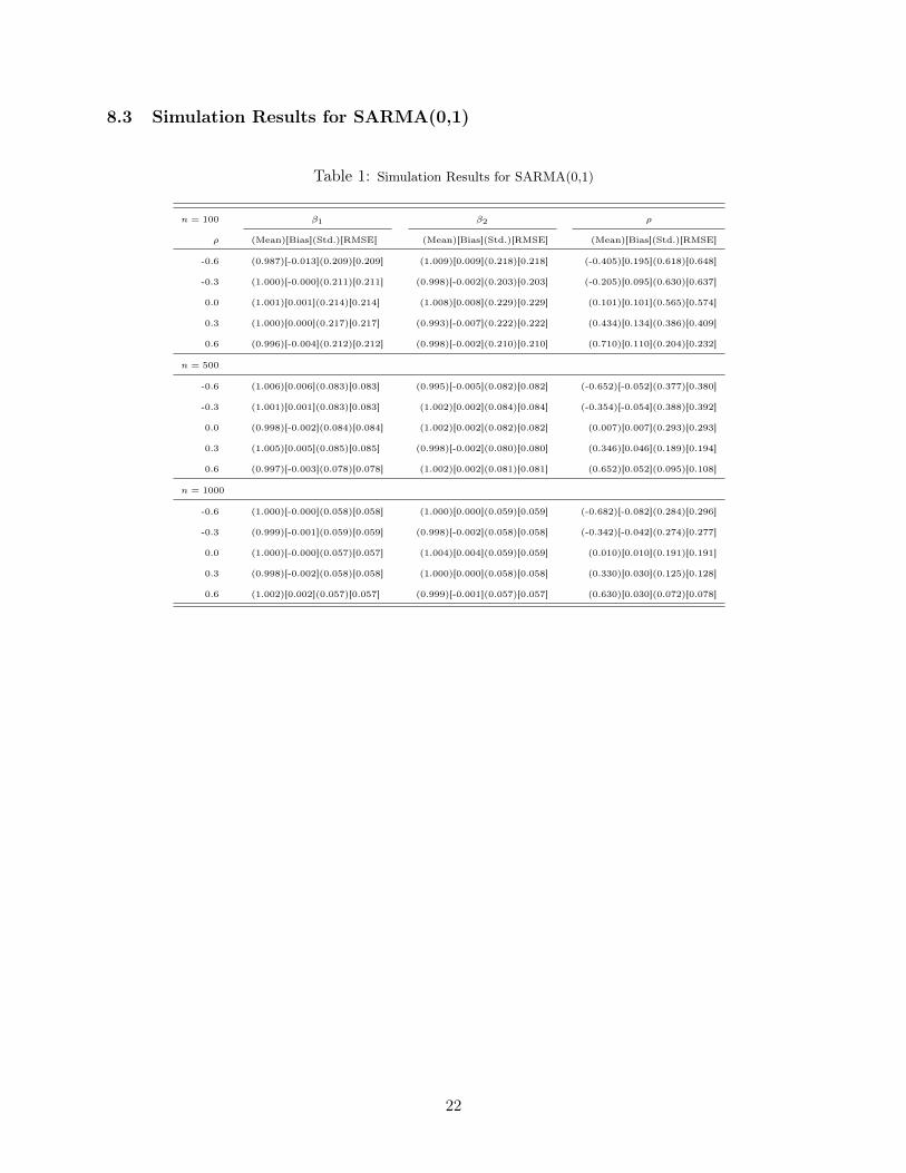
The simulation results are presented in Appendix 8.3 and 8.4. In each table, the empirical mean(Mean), the bias (Bias), the empirical standard error (Std.), and the root mean square error (RMSE)of parameter estimates are presented next to each other.

First, we consider the simulation results for the SARMA (0,1) model. The simulation results arepresented in Table 1 of Appendix 8.3. The MLE imposes almost no bias on �

10

and �20

in all cases.The moving average parameter ⇢

0

has substantial amount of bias when n = 100, but the amountof bias decreases as the sample size increases. Despite this, the MLE imposes significant amount ofbias on ⇢

0

when n = 500 and n = 1000 in cases where the true value of ⇢0

is nonzero. Overall, thesimulation results are consistent with our large sample results. That is, the MLE of �

10

and �20

isconsistent, while the MLE of ⇢

0

is inconsistent in the presence of heteroskedasticity.Now, we turn to the simulation results for the case of SARMA(1,1). First, we consider the

simulation results for �0

and ⇢0

. Table 2 shows the estimation results for n = 100. The MLEimposes substantial amount of bias on both parameters in all cases. The amount of bias for �

0

isrelatively larger when there exists a strong negative spatial dependence in the dependent variable.There is a similar pattern for ⇢

0

, where the amount of bias and RMSE is, in general, larger for the9Here, Diag (B1, . . . , BG) denotes the block diagonal matrix in which the diagonal blocks are mi ⇥ mi matrices

Bis.

16

cases of high negative spatial dependence in both dependent variable and disturbance term. Thepattern that we see for �

0

and ⇢0

shows itself for the estimation results of �10

and �20

. That is,the reported biases and RMSEs are relatively larger for �

10

and �20

, when there are strong spatialdependence in the model.

Table 3 contains the simulation results when n = 500. The same pattern that I described for�0

and ⇢0

is also prevalent in Table 3. The MLE still imposes substantial amount of bias on �0

and ⇢0

. The noticeable improvement in the estimation results for �10

and �20

suggests that theseparameters are less affected by the inconsistency of the MLE of �

0

and ⇢0

, when the sample sizeis moderately large. The estimation results in Table 4 for �

10

and �20

are also consistent with thisclaim. That is, when the sample size is large , i.e., n = 1000, the MLE imposes trivial bias on �

10

and �20

in most cases. On the other hand, the estimation results in Table 4 show that the MLEimposes significant bias on �

0

and ⇢0

, which in turn implies the inconsistency of the MLE for theseparameters.

I now evaluate the finite sample efficiency measured by RMSE of the MLE through the surfaceplots given in Appendix 8.5. Figure 3 shows the surface plots of RMSEs for �

10

and �20

. It is clearfrom the surface plots that the MLE has higher RMSEs when strong spatial dependence exists inthe model. The surface plots in Figure 4 are for �

0

and ⇢0

. These surface plots indicate that theMLE of these parameters has higher RMSEs when there exists strong negative spatial dependencein both the dependent variable and disturbance term.

7 Conclusion

In this study, I show that the MLE of the spatial autoregressive and moving average parametersfor the SARMA(1,1) specification is generally inconsistent in the presence of heteroskedastic distur-bances. The analytical results indicate that the concentrated log-likelihood function is not maxi-mized at the true parameter values when heteroskedasticity is not considered in the estimation. Thenecessary condition for the consistency of the MLE depends on the specification of spatial weightmatrices. We also show that the MLE of the parameters of the exogenous variables is inconsistent,and we state the expression for the corresponding asymptotic bias.

The Monte Carlo results show that the MLE imposes substantial amount of bias on the spatialautoregressive and moving average parameters in all cases for all sample sizes when the spatialweight matrix has non-identical blocks on the diagonals. The simulation results also show that theinconsistency of the spatial autoregressive and moving average parameters has almost no effect onthe estimates of parameters of the exogenous variables for cases where the sample size is large.

17

8 Appendix

8.1 Some Useful Lemmas

Lemma 1. Let An, Bn and Cn be n ⇥ n matrices with (i, j)th elements respectively denoted byan,ij, bn,ij and cn,ij. Assume that An and Bn have zero diagonal elements, and Cn has uniformlybounded row and column sums in absolute value. Let qn be n ⇥ 1 vector with uniformly boundedelements in absolute value. Assume that "n satisfies Assumption 1 with covariance matrix denotedby ⌃n=Diag{�2n1, . . . ,�2nn}. Then,

(1) E

⇣"0nAn"n · "0nBn"n

⌘=

nX

i=1

nX

j=1

an,ij (bn,ij + bn,ji)�2

ni�2

nj = tr

⇣⌃nAn

⇣B

0n⌃n + ⌃nBn

⌘⌘

(2) E ("nCn"n)2

=

nX

i=1

c2n,ii⇥E

�"4ni�� 3�4ni

⇤+

nX

i=1

cn,ii�2

ni

!2

+

nX

i=1

nX

j=1

cn,ij (cn,ij + cn,ji)�2

ni�2

nj

=

nX

i=1

c2n,ii⇥E

�"4ni�� 3�4ni

⇤+ tr

2

(⌃nCn) + tr

⇣⌃nCnC

0n⌃n + ⌃nCn⌃nCn

⌘,

(3) Var ("nCn"n) =nX

i=1

c2n,ii⇥E("4ni)� 3�4ni

⇤+

nX

i=1

nX

j=1

cn,ij(cn,ij + cn,ji)�2

ni�2

nj

=

nX

i=1

c2n,ii⇥E("4ni)� 3�4ni

⇤+ tr

⇣⌃nCnC

0n⌃n + ⌃nCn⌃nCn

⌘.

(4) E

⇣"0nCn"n

⌘= O(n), Var

⇣"0nCn"n

⌘= O(n), "

0nCn"n = Op(n).

(5) E (Cn"n) = 0, Var (Cn"n) = O(n), Cn"n = Op(n), Var⇣q0nCn"n

⌘= O(n), q

0nCn"n = Op(n).

Proof. For (1), (2), (3), (4) and (5) see Lemmas A.1 through A.4 in Lin and Lee (2010) and Lemma2 in Dogan and Suleyman (2013).

Lemma 2. Consider Mn = (In � Pn), where Pn = Xn(X0nXn)

�1X0n under Assumption 3. Assume

that "n satisfies Assumption 1 with covariance matrix denoted by ⌃n=Diag{�2n1, . . . ,�2nn}. Then,

(1) Mn and Pn are uniformly bounded in absolute value in both row and column sums.

(2) Var (Pn"n) = O

✓1

n

◆, Pn"n = op(1), Var ("nPn"n) = O

✓1

n

◆, "nPn"n = Op(1).

(3) Elements of Pn are O

✓1

n

◆.

Proof. The proof is similar to the proof of Lemma 3 in Dogan and Suleyman (2013). Hence, it is

18

omitted.

8.2 Proof of Proposition 1

For the probability limit of terms in (4.14), the partial derivatives @�̂2n(�)@⇢ , @�̂2

n(�)@� and @Mn(⇢)

@⇢ arerequired, which are given by

(1)

@Mn(⇢)

@⇢= �

R�1

n (⇢)MnXn(⇢)⇣X

0n(⇢)Xn(⇢)

⌘�1

X0n(⇢)

��Xn(⇢)

⇣X

0n(⇢)Xn(⇢)

⌘�1

⇥X0n(⇢)M

0nR

0�1

n (⇢)

�+

Xn(⇢)

⇣X

0n(⇢)Xn(⇢)

⌘�1

X0n(⇢)H

0n(⇢)Xn(⇢)

⇣X

0n(⇢)Xn(⇢)

⌘�1

X0n(⇢)

�

+

Xn(⇢)

⇣X

0n(⇢)Xn(⇢)

⌘�1

X0n(⇢)Hn(⇢)Xn(⇢)

⇣X

0n(⇢)Xn(⇢)

⌘�1

X0n(⇢)

�

(2)

@�̂2n(�)

@⇢=

2

nY

0nS

0n(�)H

0n(⇢)R

0�1

n (⇢)Mn(⇢)R�1

n (⇢)Sn(�)Yn

�

�2

nY

0nS

0n(�)R

0�1

n (⇢)Pn(⇢)H0nMn(⇢)R

�1

n (⇢)Sn(�)Yn

�.

(3)

@�̂2n(�)

@�= �

2

nY

0nS

0n(�)R

0�1

n (⇢)Mn(⇢)R�1

n (⇢)WnYn

�.

First, the probability limit of the first row in (4.14) is investigated:

plim

n!1

1

n

� n

2

n"0nMn"n

@�̂2n(�0)

@�

!= plim

n!1

1

n"0nMnGn"n1

n"0nMn"n

+ plim

n!1

1

n"0nMnGnXn�01

n"0nMn"n

, (8.1)

where we use X0nMn = 0k⇥n. For the second term on the r.h.s. of (8.1), we have

plim

n!1

1

n"0nMnR�1

n GnXn�01

n"0nMn"n

= 0, (8.2)

since the numerator converges in probability to zero by Lemma 1(5) and Lemma 2(1), and for theterm in the denominator we have 1

n"0nMn"n =

1

n

Pni=1

�2ni + op(1) as shown in (4.11). The overallresult is zero since 1

n

Pni=1

�2ni is uniformly bounded for all n by Assumption 1. As for the first termon the r.h.s of (8.1), we have

plim

n!1

1

n"0nMnGn"n1

n"0nMn"n

= plim

n!1

1

n"nGn"n1

n"0nMn"n

� plim

n!1

1

n"nXn

⇣X

0nXn

⌘�1

X0nGn"n

1

n"0nMn"n

. (8.3)

We first evaluate the last term in (8.3). The numerator of this term tends to zero in probabilityas n goes to infinity by Lemma 1(4) and Assumption 3. Hence, the last term in (8.3) vanishes.

19

Now, we return to the first term in the r.h.s. of (8.3). By Lemma 1(4),Var

⇣1

n"0nGn"n

⌘= O

�1

n

�= o(1). Then, the Chebyshev inequality implies that

plimn!1

⇣1

n"0nGn"n � E

⇣1

n"0nGn"n

⌘⌘= plimn!1

⇣1

n"0nGn"n � 1

n

Pni=1

Gn.ii�2ni

⌘= 0. Hence,

1

n"nGn"n1

n"0nMn"n

=

1

n

Pni=1

Gn,ii�2ni1

n

Pni=1

�2ni+ op(1). (8.4)

These results imply the following one:

1

n

� n

2

n"0nMn"n

@�̂2n(�0)

@�

!=

1

n

Pni=1

Gn.ii�2ni1

n

Pni=1

�2ni+ op(1). (8.5)

Now, we return to the first term in the second row of (4.14):

plim

n!1

1

n

� n

2

n"0nMn"n

@�̂2n(�0)

@⇢

!= � plim

n!1

1

nY0nS

0nH

0nR

0�1

n MnR�1

n SnYn1

n"0nMn"n

+ plim

n!1

1

nY0nS

0nR

0�1

n PnH0nMnR�1

n SnYn1

n"0nMn"n

. (8.6)

Each term is handled separately below by using R�1

n SnYn = Xn�0 + "n, SnYn = Xn�0 + Rn"n,X

0nMn = 0k⇥n and MnXn = 0n⇥k. Note that 1

nY0nS

0nR

0�1

n PnH0nMnR�1

n SnYn =

1

n�00

X0nPnH

0nMn"n+

1

n"nPnH0nMn"n. By Lemma 1(5) and Lemma 2(1), 1

n�00

X0nH

0nMn"n = op(1). By Lemma 1(4)

and Assumption 3, we have 1

n"0nPnHn"n = op(1). For the remaining term, by Lemma 2, we have

1

n"nPnH0nMn"n = op(1). Hence, the second term on the r.h.s. of (8.6) vanishes.

The first term on r.h.s. of (8.6) can be written as

� plim

n!1

1

nY0nS

0nR

0�1

n MnHnR�1

n SnYn1

n"0nMn"n

= � plim

n!1

1

n"0nMnHnXn�01

n"0nMn"n

� plim

n!1

1

n"0nMnHn"n1

n"0nMn"n

. (8.7)

Substituting Mn = In �Xn

⇣X

0nXn

⌘�1

X0n into (8.7) yields

� plim

n!1

1

nY0nS

0nR

0�1

n MnHnR�1

n SnYn1

n"0nMn"n

= � plim

n!1

1

n"0nHn"n

1

n"0nMn"n

� plim

n!1

1

n"0nMnHnXn�01

n"0nMn"n

+ plim

n!1

1

n2 "0nXn

⇣1

nX0nXn

⌘�1

X0nHn"n

1

n"0nMn"n

. (8.8)

By Lemma 1(5) and (4.11), the second term on the r.h.s of (8.8) vanishes. The third term vanishes byLemma 1(4) and (4.11). The probability limit of the remaining term can be found by the Chebyshevinequality. By Lemma 1(4), we have Var

⇣1

n"0nHn"n

⌘= O(

1

n) = o(1). Hence, plimn!1�1

n"0nHn"n�

E(

1

n"0nHn"n)

�= plimn!1

�1

n"0nHn"n � 1

n

Pni=1

Hn,ii�2ni�= 0. Combining these results, we get the

20

following result for the first term in the first row of (4.14):

1

n

� n

2

n"0nMn"n

@�̂2n(�0)

@⇢

!= �

1

n

Pni=1

Hn,ii�2ni1

n

Pni=1

�2ni+ op(1). (8.9)

By combining the results in (8.5) and (8.9), we obtain:

1

n

@ lnLn(�0)

@�=

0

BBB@

1n

Pni=1 Gn.ii�

2ni

1n

Pni=1 �

2ni

� 1

n tr(Gn) + op(1)

�⇣ 1

n

Pni=1 Hn,ii�

2ni

1n

Pni=1 �

2ni

� 1

n tr(Hn)

⌘+ op(1)

1

CCCA. (8.10)

For the notational simplification, denote H⇤n =

1

n tr(Hn) =

1

n

Pni=1

Hn,ii, G⇤n =

1

n tr(Gn) =

1

n

Pni=1

Gn,ii, and �2 = 1

n

Pni=1

�2ni. Then, (8.10) can be written in a more convenient form as10

1

n

@ lnLn(�0)

@�=

0

BBBB@

1n

Pni=1

�Gn.ii�G⇤

� ��2ni��2

�

�2 � 1

n tr(Gn �Gn) + op(1)

�1n

Pni=1

�Hn,ii�H⇤

n

� ��2ni��2

�

�2 + op(1)

1

CCCCA

=

0

BBBB@

cov

(

Gn,ii, �2ni)

�2 + op(1)

� cov

(

Hn,ii, �2ni)

�2 + op(1)

1

CCCCA. (8.11)

10Note that 1n tr(Gn �Gn) = 0.

21

8.3 Simulation Results for SARMA(0,1)

Table 1: Simulation Results for SARMA(0,1)

n = 100 �1 �2 ⇢

⇢ (Mean)[Bias](Std.)[RMSE] (Mean)[Bias](Std.)[RMSE] (Mean)[Bias](Std.)[RMSE]

-0.6 (0.987)[-0.013](0.209)[0.209] (1.009)[0.009](0.218)[0.218] (-0.405)[0.195](0.618)[0.648]

-0.3 (1.000)[-0.000](0.211)[0.211] (0.998)[-0.002](0.203)[0.203] (-0.205)[0.095](0.630)[0.637]

0.0 (1.001)[0.001](0.214)[0.214] (1.008)[0.008](0.229)[0.229] (0.101)[0.101](0.565)[0.574]

0.3 (1.000)[0.000](0.217)[0.217] (0.993)[-0.007](0.222)[0.222] (0.434)[0.134](0.386)[0.409]

0.6 (0.996)[-0.004](0.212)[0.212] (0.998)[-0.002](0.210)[0.210] (0.710)[0.110](0.204)[0.232]

n = 500

-0.6 (1.006)[0.006](0.083)[0.083] (0.995)[-0.005](0.082)[0.082] (-0.652)[-0.052](0.377)[0.380]

-0.3 (1.001)[0.001](0.083)[0.083] (1.002)[0.002](0.084)[0.084] (-0.354)[-0.054](0.388)[0.392]

0.0 (0.998)[-0.002](0.084)[0.084] (1.002)[0.002](0.082)[0.082] (0.007)[0.007](0.293)[0.293]

0.3 (1.005)[0.005](0.085)[0.085] (0.998)[-0.002](0.080)[0.080] (0.346)[0.046](0.189)[0.194]

0.6 (0.997)[-0.003](0.078)[0.078] (1.002)[0.002](0.081)[0.081] (0.652)[0.052](0.095)[0.108]

n = 1000

-0.6 (1.000)[-0.000](0.058)[0.058] (1.000)[0.000](0.059)[0.059] (-0.682)[-0.082](0.284)[0.296]

-0.3 (0.999)[-0.001](0.059)[0.059] (0.998)[-0.002](0.058)[0.058] (-0.342)[-0.042](0.274)[0.277]

0.0 (1.000)[-0.000](0.057)[0.057] (1.004)[0.004](0.059)[0.059] (0.010)[0.010](0.191)[0.191]

0.3 (0.998)[-0.002](0.058)[0.058] (1.000)[0.000](0.058)[0.058] (0.330)[0.030](0.125)[0.128]

0.6 (1.002)[0.002](0.057)[0.057] (0.999)[-0.001](0.057)[0.057] (0.630)[0.030](0.072)[0.078]

22

8.4 Simulation Results for SARMA(1,1)

Table 2: Simulation Results for SARMA(1,1): n = 100

� �1 �2 ⇢

� ⇢ (Mean)[Bias](Std.)[RMSE] (Mean)[Bias](Std.)[RMSE] (Mean)[Bias](Std.)[RMSE] (Mean)[Bias](Std.)[RMSE]

-0.6 -0.6 (-1.583)[-0.983](4.262)[4.374] (0.874)[-0.126](0.342)[0.364] (0.898)[-0.102](0.350)[0.365] (-0.273)[0.327](0.981)[1.034]

-0.6 -0.3 (-1.790)[-1.190](4.346)[4.506] (0.848)[-0.152](0.371)[0.401] (0.847)[-0.153](0.361)[0.392] (-0.178)[0.122](0.997)[1.004]

-0.6 0.0 (-1.794)[-1.194](4.355)[4.516] (0.867)[-0.133](0.357)[0.381] (0.865)[-0.135](0.353)[0.378] (0.021)[0.021](0.934)[0.934]

-0.6 0.3 (-1.404)[-0.804](3.687)[3.773] (0.839)[-0.161](0.379)[0.412] (0.851)[-0.149](0.382)[0.410] (0.264)[-0.036](0.709)[0.710]

-0.6 0.6 (-0.591)[0.009](1.108)[1.108] (0.760)[-0.240](0.455)[0.515] (0.760)[-0.240](0.455)[0.515] (0.470)[-0.130](0.342)[0.366]

-0.3 -0.6 (-0.907)[-0.607](3.275)[3.331] (0.912)[-0.088](0.325)[0.337] (0.907)[-0.093](0.324)[0.337] (-0.259)[0.341](0.822)[0.890]

-0.3 -0.3 (-1.132)[-0.832](3.497)[3.594] (0.882)[-0.118](0.351)[0.370] (0.881)[-0.119](0.362)[0.381] (-0.136)[0.164](0.906)[0.920]

-0.3 0.0 (-1.335)[-1.035](3.840)[3.977] (0.857)[-0.143](0.361)[0.388] (0.861)[-0.139](0.367)[0.393] (-0.005)[-0.005](0.861)[0.861]

-0.3 0.3 (-1.045)[-0.745](3.364)[3.445] (0.840)[-0.160](0.399)[0.430] (0.835)[-0.165](0.400)[0.433] (0.220)[-0.080](0.709)[0.714]

-0.3 0.6 (-0.574)[-0.274](1.873)[1.893] (0.768)[-0.232](0.466)[0.521] (0.758)[-0.242](0.459)[0.519] (0.436)[-0.164](0.390)[0.423]

0.0 -0.6 (-0.452)[-0.452](2.570)[2.609] (0.904)[-0.096](0.354)[0.367] (0.898)[-0.102](0.350)[0.365] (-0.292)[0.308](0.721)[0.784]

0.0 -0.3 (-0.690)[-0.690](3.123)[3.199] (0.903)[-0.097](0.337)[0.350] (0.889)[-0.111](0.340)[0.358] (-0.208)[0.092](0.772)[0.778]

0.0 0.0 (-0.834)[-0.834](3.174)[3.282] (0.841)[-0.159](0.383)[0.415] (0.857)[-0.143](0.391)[0.416] (-0.079)[-0.079](0.804)[0.808]

0.0 0.3 (-0.450)[-0.450](2.131)[2.178] (0.839)[-0.161](0.407)[0.438] (0.838)[-0.162](0.412)[0.442] (0.238)[-0.062](0.590)[0.593]

0.0 0.6 (-0.278)[-0.278](1.068)[1.104] (0.768)[-0.232](0.469)[0.523] (0.763)[-0.237](0.463)[0.521] (0.411)[-0.189](0.349)[0.397]

0.3 -0.6 (0.068)[-0.232](1.429)[1.448] (0.938)[-0.062](0.311)[0.317] (0.951)[-0.049](0.307)[0.311] (-0.384)[0.216](0.543)[0.585]

0.3 -0.3 (-0.157)[-0.457](2.174)[2.221] (0.903)[-0.097](0.344)[0.358] (0.902)[-0.098](0.345)[0.359] (-0.279)[0.021](0.623)[0.623]

0.3 0.0 (-0.211)[-0.511](2.030)[2.094] (0.867)[-0.133](0.376)[0.399] (0.864)[-0.136](0.381)[0.404] (-0.161)[-0.161](0.660)[0.679]

0.3 0.3 (-0.203)[-0.503](2.007)[2.069] (0.819)[-0.181](0.437)[0.473] (0.813)[-0.187](0.432)[0.471] (0.095)[-0.205](0.621)[0.654]

0.3 0.6 (-0.022)[-0.322](0.735)[0.802] (0.659)[-0.341](0.508)[0.612] (0.657)[-0.343](0.503)[0.609] (0.329)[-0.271](0.381)[0.468]

0.6 -0.6 (0.422)[-0.178](0.712)[0.733] (0.981)[-0.019](0.231)[0.232] (0.981)[-0.019](0.230)[0.231] (-0.584)[0.016](0.346)[0.346]

0.6 -0.3 (0.376)[-0.224](0.580)[0.621] (0.976)[-0.024](0.253)[0.254] (0.965)[-0.035](0.255)[0.257] (-0.511)[-0.211](0.329)[0.391]

0.6 0.0 (0.270)[-0.330](0.842)[0.905] (0.961)[-0.039](0.294)[0.296] (0.945)[-0.055](0.292)[0.297] (-0.412)[-0.412](0.386)[0.564]

0.6 0.3 (0.152)[-0.448](1.345)[1.418] (0.921)[-0.079](0.326)[0.335] (0.920)[-0.080](0.335)[0.344] (-0.286)[-0.586](0.415)[0.719]

0.6 0.6 (0.159)[-0.441](0.767)[0.884] (0.802)[-0.198](0.436)[0.479] (0.800)[-0.200](0.432)[0.476] (-0.059)[-0.659](0.414)[0.779]

23

Table 3: Simulation Results for SARMA(1,1): n = 500

� �1 �2 ⇢

� ⇢ (Mean)[Bias](Std.)[RMSE] (Mean)[Bias](Std.)[RMSE] (Mean)[Bias](Std.)[RMSE] (Mean)[Bias](Std.)[RMSE]

-0.6 -0.6 (-3.051)[-2.451](7.286)[7.687] (0.914)[-0.086](0.257)[0.271] (0.911)[-0.089](0.256)[0.271] (-1.040)[-0.440](1.921)[1.970]

-0.6 -0.3 (-2.905)[-2.305](7.213)[7.572] (0.916)[-0.084](0.253)[0.267] (0.918)[-0.082](0.254)[0.267] (-0.725)[-0.425](1.913)[1.960]

-0.6 0.0 (-1.771)[-1.171](5.677)[5.797] (0.953)[-0.047](0.203)[0.208] (0.949)[-0.051](0.204)[0.210] (-0.123)[-0.123](1.427)[1.432]

-0.6 0.3 (-0.977)[-0.377](3.577)[3.597] (0.985)[-0.015](0.142)[0.143] (0.982)[-0.018](0.140)[0.141] (0.303)[0.003](0.814)[0.814]

-0.6 0.6 (-0.667)[-0.067](0.139)[0.154] (1.003)[0.003](0.088)[0.088] (1.006)[0.006](0.085)[0.085] (0.609)[0.009](0.087)[0.087]

-0.3 -0.6 (-0.985)[-0.685](4.189)[4.244] (0.979)[-0.021](0.163)[0.165] (0.975)[-0.025](0.162)[0.164] (-0.608)[-0.008](1.201)[1.201]

-0.3 -0.3 (-1.513)[-1.213](5.164)[5.304] (0.953)[-0.047](0.187)[0.193] (0.960)[-0.040](0.189)[0.193] (-0.577)[-0.277](1.472)[1.498]

-0.3 0.0 (-1.196)[-0.896](4.602)[4.689] (0.972)[-0.028](0.174)[0.177] (0.968)[-0.032](0.171)[0.174] (-0.155)[-0.155](1.284)[1.293]

-0.3 0.3 (-0.457)[-0.157](1.797)[1.804] (0.996)[-0.004](0.103)[0.103] (0.994)[-0.006](0.102)[0.102] (0.312)[0.012](0.449)[0.449]

-0.3 0.6 (-0.460)[-0.160](0.212)[0.266] (1.000)[-0.000](0.082)[0.082] (1.006)[0.006](0.082)[0.082] (0.557)[-0.043](0.132)[0.139]

0.0 -0.6 (0.040)[0.040](1.086)[1.087] (0.998)[-0.002](0.090)[0.090] (0.998)[-0.002](0.086)[0.086] (-0.371)[0.229](0.468)[0.521]

0.0 -0.3 (-0.220)[-0.220](2.089)[2.100] (0.994)[-0.006](0.103)[0.103] (0.994)[-0.006](0.109)[0.109] (-0.333)[-0.033](0.703)[0.704]

0.0 0.0 (-0.205)[-0.205](1.807)[1.819] (0.996)[-0.004](0.101)[0.101] (0.995)[-0.005](0.101)[0.101] (-0.075)[-0.075](0.681)[0.685]

0.0 0.3 (-0.077)[-0.077](0.731)[0.735] (0.996)[-0.004](0.085)[0.085] (0.998)[-0.002](0.087)[0.087] (0.298)[-0.002](0.328)[0.328]

0.0 0.6 (-0.153)[-0.153](0.253)[0.296] (0.987)[-0.013](0.136)[0.137] (0.989)[-0.011](0.135)[0.136] (0.521)[-0.079](0.197)[0.213]

0.3 -0.6 (0.317)[0.017](0.140)[0.141] (1.003)[0.003](0.084)[0.084] (1.000)[0.000](0.082)[0.082] (-0.430)[0.170](0.201)[0.263]

0.3 -0.3 (0.228)[-0.072](0.173)[0.188] (1.003)[0.003](0.086)[0.086] (0.998)[-0.002](0.083)[0.083] (-0.323)[-0.023](0.272)[0.273]

0.3 0.0 (0.137)[-0.163](0.715)[0.734] (0.998)[-0.002](0.086)[0.087] (0.997)[-0.003](0.086)[0.086] (-0.174)[-0.174](0.408)[0.444]

0.3 0.3 (0.199)[-0.101](0.211)[0.234] (0.996)[-0.004](0.100)[0.100] (0.996)[-0.004](0.100)[0.100] (0.216)[-0.084](0.362)[0.372]

0.3 0.6 (0.245)[-0.055](0.194)[0.202] (0.961)[-0.039](0.211)[0.214] (0.958)[-0.042](0.209)[0.213] (0.587)[-0.013](0.205)[0.205]

0.6 -0.6 (0.545)[-0.055](0.086)[0.102] (0.998)[-0.002](0.082)[0.082] (1.000)[-0.000](0.084)[0.084] (-0.652)[-0.052](0.102)[0.115]

0.6 -0.3 (0.486)[-0.114](0.082)[0.141] (0.998)[-0.002](0.082)[0.082] (1.001)[0.001](0.081)[0.081] (-0.583)[-0.283](0.103)[0.301]

0.6 0.0 (0.411)[-0.189](0.091)[0.209] (1.000)[0.000](0.083)[0.083] (0.997)[-0.003](0.081)[0.081] (-0.490)[-0.490](0.124)[0.505]

0.6 0.3 (0.324)[-0.276](0.088)[0.290] (1.007)[0.007](0.089)[0.090] (1.003)[0.003](0.092)[0.092] (-0.344)[-0.644](0.200)[0.674]

0.6 0.6 (0.288)[-0.312](0.159)[0.350] (0.943)[-0.057](0.253)[0.259] (0.941)[-0.059](0.253)[0.260] (-0.070)[-0.670](0.387)[0.774]

24

Table 4: Simulation Results for SARMA(1,1): n = 1000

� �1 �2 ⇢

� ⇢ (Mean)[Bias](Std.)[RMSE] (Mean)[Bias](Std.)[RMSE] (Mean)[Bias](Std.)[RMSE] (Mean)[Bias](Std.)[RMSE]

-0.6 -0.6 (-3.449)[-2.849](8.618)[9.077] (0.907)[-0.093](0.283)[0.298] (0.906)[-0.094](0.282)[0.297] (-1.323)[-0.723](2.487)[2.590]

-0.6 -0.3 (-4.151)[-3.551](9.648)[10.280] (0.877)[-0.123](0.311)[0.334] (0.880)[-0.120](0.312)[0.335] (-1.135)[-0.835](2.798)[2.920]

-0.6 0.0 (-1.675)[-1.075](6.110)[6.204] (0.957)[-0.043](0.201)[0.205] (0.958)[-0.042](0.199)[0.204] (-0.148)[-0.148](1.666)[1.672]

-0.6 0.3 (-0.650)[-0.050](2.400)[2.401] (0.991)[-0.009](0.092)[0.093] (0.991)[-0.009](0.093)[0.093] (0.352)[0.052](0.568)[0.570]

-0.6 0.6 (-0.682)[-0.082](0.095)[0.126] (1.007)[0.007](0.059)[0.060] (1.007)[0.007](0.057)[0.058] (0.595)[-0.005](0.054)[0.055]

-0.3 -0.6 (-0.698)[-0.398](3.631)[3.653] (0.983)[-0.017](0.128)[0.129] (0.985)[-0.015](0.129)[0.129] (-0.624)[-0.024](1.152)[1.153]

-0.3 -0.3 (-1.691)[-1.391](6.083)[6.240] (0.952)[-0.048](0.204)[0.210] (0.954)[-0.046](0.204)[0.209] (-0.704)[-0.404](1.839)[1.883]

-0.3 0.0 (-0.829)[-0.529](4.086)[4.120] (0.981)[-0.019](0.141)[0.143] (0.982)[-0.018](0.142)[0.143] (-0.103)[-0.103](1.241)[1.245]

-0.3 0.3 (-0.385)[-0.085](1.415)[1.418] (1.000)[-0.000](0.073)[0.073] (0.999)[-0.001](0.074)[0.074] (0.300)[-0.000](0.335)[0.335]

-0.3 0.6 (-0.476)[-0.176](0.169)[0.244] (1.005)[0.005](0.058)[0.058] (1.007)[0.007](0.058)[0.058] (0.524)[-0.076](0.105)[0.130]

0.0 -0.6 (0.090)[0.090](0.866)[0.870] (0.998)[-0.002](0.064)[0.064] (1.000)[-0.000](0.067)[0.067] (-0.361)[0.239](0.373)[0.443]

0.0 -0.3 (-0.096)[-0.096](1.508)[1.511] (0.996)[-0.004](0.083)[0.083] (0.995)[-0.005](0.078)[0.078] (-0.323)[-0.023](0.575)[0.575]

0.0 0.0 (-0.111)[-0.111](1.287)[1.291] (0.997)[-0.003](0.071)[0.071] (0.994)[-0.006](0.070)[0.070] (-0.063)[-0.063](0.525)[0.529]

0.0 0.3 (-0.074)[-0.074](0.181)[0.195] (0.997)[-0.003](0.060)[0.060] (0.999)[-0.001](0.060)[0.060] (0.260)[-0.040](0.169)[0.174]

0.0 -0.6 (0.068)[-0.232](1.429)[1.448] (0.938)[-0.062](0.311)[0.317] (0.951)[-0.049](0.307)[0.311] (-0.384)[0.216](0.543)[0.585]

0.3 -0.6 (0.342)[0.042](0.090)[0.099] (1.000)[0.000](0.060)[0.060] (1.001)[0.001](0.059)[0.059] (-0.429)[0.171](0.118)[0.208]

0.3 -0.3 (0.251)[-0.049](0.111)[0.121] (1.000)[-0.000](0.063)[0.063] (1.004)[0.004](0.060)[0.061] (-0.338)[-0.038](0.152)[0.157]

0.3 0.0 (0.174)[-0.126](0.125)[0.178] (1.001)[0.001](0.058)[0.058] (0.998)[-0.002](0.059)[0.059] (-0.188)[-0.188](0.229)[0.296]

0.3 0.3 (0.225)[-0.075](0.145)[0.163] (0.999)[-0.001](0.061)[0.061] (0.999)[-0.001](0.058)[0.058] (0.223)[-0.077](0.271)[0.281]

0.3 0.6 (0.274)[-0.026](0.147)[0.149] (0.996)[-0.004](0.097)[0.097] (0.992)[-0.008](0.097)[0.097] (0.609)[0.009](0.148)[0.148]

0.6 -0.6 (0.562)[-0.038](0.055)[0.067] (1.002)[0.002](0.059)[0.059] (1.000)[0.000](0.059)[0.059] (-0.668)[-0.068](0.066)[0.095]

0.6 -0.3 (0.496)[-0.104](0.058)[0.119] (1.002)[0.002](0.059)[0.059] (1.000)[0.000](0.058)[0.058] (-0.590)[-0.290](0.071)[0.299]

0.6 0.0 (0.417)[-0.183](0.058)[0.192] (0.998)[-0.002](0.062)[0.062] (1.000)[0.000](0.061)[0.061] (-0.495)[-0.495](0.072)[0.501]

0.6 0.3 (0.324)[-0.276](0.061)[0.282] (1.004)[0.004](0.060)[0.060] (1.002)[0.002](0.060)[0.060] (-0.372)[-0.672](0.114)[0.682]

0.6 0.6 (0.320)[-0.280](0.176)[0.331] (0.977)[-0.023](0.175)[0.177] (0.975)[-0.025](0.176)[0.177] (0.007)[-0.593](0.416)[0.725]

25

8.5 Surface Plots of RMSEs for SARMA(1,1)

Figure 3: RMSE of �1

and �2

−0.6−0.3

00.3

0.6

−0.6

−0.3

0

0.3

0.6

0.25

0.3

0.35

0.4

0.45

0.5

0.55

0.6

λρ

RM

SE

0.25

0.3

0.35

0.4

0.45

0.5

0.55

0.6

(a) �1, n = 100

−0.6−0.3

00.3

0.6

−0.6

−0.3

0

0.3

0.6

0.25

0.3

0.35

0.4

0.45

0.5

0.55

0.6

λρ

RM

SE

0.25

0.3

0.35

0.4

0.45

0.5

0.55

0.6

(b) �2, n = 100

−0.6−0.3

00.3

0.6

−0.6

−0.3

0

0.3

0.6

0.1

0.12

0.14

0.16

0.18

0.2

0.22

0.24

0.26

λρ

RM

SE

0.1

0.12

0.14

0.16

0.18

0.2

0.22

0.24

0.26

(c) �1, n = 500

−0.6−0.3

00.3

0.6

−0.6

−0.3

0

0.3

0.6

0.1

0.12

0.14

0.16

0.18

0.2

0.22

0.24

0.26

λρ

RM

SE

0.1

0.12

0.14

0.16

0.18

0.2

0.22

0.24

0.26

(d) �2, n = 500

−0.6−0.3

00.3

0.6

−0.6

−0.3

0

0.3

0.6

0.1

0.15

0.2

0.25

0.3

λρ

RM

SE

0.1

0.15

0.2

0.25

0.3

(e) �1, n = 1000

−0.6−0.3

00.3

0.6

−0.6

−0.3

0

0.3

0.6

0.1

0.15

0.2

0.25

0.3

λρ

RM

SE

0.1

0.15

0.2

0.25

0.3

(f) �2, n = 1000

26

Figure 4: RMSE of � and ⇢

−0.6−0.3

00.3

0.6

−0.6

−0.3

0

0.3

0.6

1

1.5

2

2.5

3

3.5

4

4.5

λρ

RM

SE

1

1.5

2

2.5

3

3.5

4

4.5

(a) �, n = 100

−0.6−0.3

00.3

0.6

−0.6

−0.3

0

0.3

0.6

0.4

0.5

0.6

0.7

0.8

0.9

1

λρ

RM

SE

0.4

0.5

0.6

0.7

0.8

0.9

1

(b) ⇢, n = 100

−0.6−0.3

00.3

0.6

−0.6

−0.3

0

0.3

0.6

1

2

3

4

5

6

7

λρ

RM

SE

1

2

3

4

5

6

7

(c) �, n = 500

−0.6−0.3

00.3

0.6

−0.6

−0.3

0

0.3

0.6

0.2

0.4

0.6

0.8

1

1.2

1.4

1.6

1.8

λρ

RM

SE

0.2

0.4

0.6

0.8

1

1.2

1.4

1.6

1.8

(d) ⇢, n = 500

−0.6−0.3

00.3

0.6

−0.6

−0.3

0

0.3

0.6

1

2

3

4

5

6

7

8

9

10

λρ

RM

SE

1

2

3

4

5

6

7

8

9

10

(e) �, n = 1000

−0.6−0.3

00.3

0.6

−0.6

−0.3

0

0.3

0.6

0.5

1

1.5

2

2.5

λρ

RM

SE

0.5

1

1.5

2

2.5

(f) ⇢, n = 1000

27

References

Abadir, Karim M. and Jan R. Magnus (2005). Matrix Algebra. Econometric Exercises. New York:Cambridge University Press.

Anselin, Luc (1988). Spatial econometrics: Methods and Models. New York: Springer.Arnold, Matthias and Dominik Wied (2010). “Improved GMM estimation of the spatial autoregres-

sive error model”. In: Economics Letters 108.1, pp. 65 –68.Baltagi, Badi H. and Long Liu (2011). “An improved generalized moments estimator for a spatial

moving average error model”. In: Economics Letters 113.3, pp. 282 –284.Besag, Julian (1974). “Spatial Interaction and the Statistical Analysis of Lattice Systems”. In: Jour-

nal of the Royal Statistical Society. Series B (Methodological) 36.2, pp. 192–236.Das, Debabrata, Harry H. Kelejian, and Ingmar R. Prucha (2003). “Small Sample Properties of

Estimators of Spatial Autoregressive Models with Autoregressive Disturbances”. In: Papers inRegional Science 82, pp. 1–26.

Dogan, Osman and Taspinar Suleyman (2013). GMM Estimation of Spatial Autoregressive Modelswith Autoregressive and Heteroskedastic Disturbances. Working Papers 001. City University ofNew York Graduate Center, Ph.D. Program in Economics.

Drukker, David M., Peter Egger, and Ingmar R. Prucha (2013). “On Two-Step Estimation of aSpatial Autoregressive Model with Autoregressive Disturbances and Endogenous Regressors”.In: Econometric Reviews 32.5-6, pp. 686–733.

Fingleton, Bernard (2008a). “A generalized method of moments estimator for a spatial model withmoving average errors, with application to real estate prices”. In: Empirical Economics 34 (1),pp. 35–37.

— (2008b). “A Generalized Method of Moments Estimator for a Spatial Panel Model with anEndogenous Spatial Lag and Spatial Moving Average Errors”. In: Spatial Economic Analysis3.1, pp. 27–44.

Haining, R. P. (1978). “The Moving Average Model for Spatial Interaction”. In: Transactions of theInstitute of British Geographers. New Series 3.2, pp. 202–225.

Haining, Robert (1987). “Trend-Surface Models with Regional and Local Scales of Variation withan Application to Aerial Survey Data”. In: Technometrics 29.4, pp. 461–469.

Hepple, Leslie W. (1976). “A Maximum Likelihood Model for Econometric Estimation with SpatialSeries”. In: Theory and practice in regional science. Ed. by Ian Masser. London papers in regionalscience 6. London: Pion Limited.

— (1995a). “Bayesian techniques in spatial and network econometrics: 1. Model comparison andposterior odds”. In: Environment and Planning 27.3, pp. 247–469.

— (1995b). “Bayesian techniques in spatial and network econometrics: 2. Computational methodsand algorithms”. In: Environment and Planning 27.4, pp. 615–644.

— (2003). Bayesian and maximum likelihood estimation of the linear model with spatial movingaverage disturbances. School of Geographical Sciences, University of Bristol, Working PapersSeries.

28

Kelejian, Harry H. and Ingmar R. Prucha (1998). “A Generalized Spatial Two-Stage Least SquaresProcedure for Estimating a Spatial Autoregressive Model with Autoregressive Disturbances”. In:Journal of Real Estate Finance and Economics 17.1, pp. 1899–1926.

— (1999). “A Generalized Moments Estimator for the Autoregressive Parameter in a SpatialModel”. In: International Economic Review 40.2, pp. 509–533.

— (2007). “Specification and estimation of spatial autoregressive models with autoregressive andheteroskedastic disturbances, Department of Economics, University of Maryland”.

— (2010). “Specification and estimation of spatial autoregressive models with autoregressive andheteroskedastic disturbances”. In: Journal of Econometrics 157, pp. 53–67.

Kelejian, Harry H. and D Robinson (1993). “A Suggested Method of Estimation for Spatial Inter-dependent Models with Autocorrelated Errors, and an Application to a County ExpenditureModel”. In: Papers in Regional Science 72, pp. 297–312.

Lee, Lung-fei (2004). “Asymptotic Distributions of Quasi-Maximum Likelihood Estimators for Spa-tial Autoregressive Models”. In: Econometrica 72.6, pp. 1899–1925.

— (2007a). “GMM and 2SLS estimation of mixed regressive, spatial autoregressive models”. In:Journal of Econometrics 137.2, pp. 489–514.

— (2007b). “Identification and estimation of econometric models with group interactions, contex-tual factors and fixed effects”. In: Journal of Econometrics 140, pp. 333–374.

— (2007c). “The Method of Elimination and Substitution in the GMM Estimation of Mixed Re-gressive, Spatial Autoregressive Models”. In: Journal of Econometrics 140, pp. 155–189.

Lee, Lung-fei and Xiaodong Liu (2010). “Efficient GMM Estimation Of High Order Spatial Autore-gressive Models With Autoregressive Disturbances”. In: Econometric Theory 26.01, pp. 187–230.

Lee, Lung-fei, Xiaodong Liu, and Xu Lin (2010). “Specification and estimation of social interactionmodels with network structures”. In: The Econometrics Journal 13, pp. 145–176.

LeSage, James and Robert K. Pace (2009). Introduction to Spatial Econometrics (Statistics: A Seriesof Textbooks and Monographs. London: Chapman and Hall/CRC.

Lesage, James P. (1997). “Bayesian Estimation of Spatial Autoregressive Models”. In: InternationalRegional Science Review 20.1-2, pp. 113–129.

Lin, Xu and Lung-fei Lee (2010). “GMM estimation of spatial autoregressive models with unknownheteroskedasticity”. In: Journal of Econometrics 157.1, pp. 34–52.

Liu, Xiaodong, Lung-fei Lee, and Christopher R. Bollinger (2010). “An efficient GMM estimator ofspatial autoregressive models”. In: Journal of Econometrics 159.2, pp. 303–319.

Mardia, K. V. and R. J. Marshall (1984). “Maximum Likelihood Estimation of Models for ResidualCovariance in Spatial Regression”. In: Biometrika 71.1, pp. 135–146.

Pace, Robert K., James P. LeSage, and Shuang Zhu (2012). “Spatial Dependence in Regressors andits Effect on Performance of Likelihood-Based and Instrumental Variable Estimators”. In: ed. byDaniel Millimet Dek Terrell. 30th Anniversary Edition (Advances in Econometrics, Volume 30).Emerald Group Publishing Limited, pp. 257–295.

29

Prucha, Ingmar R. (2014). “Instrumental Variables/Method of Moments Estimation”. In: Handbookof Regional Science. Ed. by Manfred M. Fischer and Peter Nijkamp. Springer Berlin Heidelberg,pp. 1597–1617.

Richardson, S., C. Guihenneuc, and V. Lasserre (1992). “Spatial Linear Models with AutocorrelatedError Structure”. In: Journal of the Royal Statistical Society. Series D (The Statistician) 41.5,pp. 539–557.

Ripley, Brian D. (2005). Spatial Statistics. Wiley Series in Probability and Statistics. John Wiley &Sons.

30