Heteroskedasticity in Multiple Regression Analysis: What ...

Practical Assessment, Research, and Evaluation Practical Assessment, Research, and Evaluation

Volume 24 Volume 24, 2019 Article 1

2019

Heteroskedasticity in Multiple Regression Analysis: What it is, Heteroskedasticity in Multiple Regression Analysis: What it is,

How to Detect it and How to Solve it with Applications in R and How to Detect it and How to Solve it with Applications in R and

SPSS SPSS

Oscar L. Olvera Astivia

Bruno D. Zumbo

Follow this and additional works at: https://scholarworks.umass.edu/pare

Recommended Citation Recommended Citation Astivia, Oscar L. Olvera and Zumbo, Bruno D. (2019) "Heteroskedasticity in Multiple Regression Analysis: What it is, How to Detect it and How to Solve it with Applications in R and SPSS," Practical Assessment, Research, and Evaluation: Vol. 24 , Article 1. DOI: https://doi.org/10.7275/q5xr-fr95 Available at: https://scholarworks.umass.edu/pare/vol24/iss1/1

This Article is brought to you for free and open access by ScholarWorks@UMass Amherst. It has been accepted for inclusion in Practical Assessment, Research, and Evaluation by an authorized editor of ScholarWorks@UMass Amherst. For more information, please contact [email protected].

https://scholarworks.umass.edu/pare

https://scholarworks.umass.edu/pare/vol24

https://scholarworks.umass.edu/pare/vol24/iss1/1

https://scholarworks.umass.edu/pare?utm_source=scholarworks.umass.edu%2Fpare%2Fvol24%2Fiss1%2F1&utm_medium=PDF&utm_campaign=PDFCoverPages

https://scholarworks.umass.edu/pare/vol24/iss1/1?utm_source=scholarworks.umass.edu%2Fpare%2Fvol24%2Fiss1%2F1&utm_medium=PDF&utm_campaign=PDFCoverPages

mailto:[email protected]

A peer-reviewed electronic journal.

Copyright is retained by the first or sole author, who grants right of first publication to Practical Assessment, Research & Evaluation. Permission is granted to distribute this article for nonprofit, educational purposes if it is copied in its entirety and the journal is credited. PARE has the right to authorize third party reproduction of this article in print, electronic and database forms.

Volume 24 Number 1, January 2019 ISSN 1531-7714

Heteroskedasticity in Multiple Regression Analysis: What it is, How to Detect it and How to Solve it with

Applications in R and SPSS Oscar L. Olvera Astivia, University of British Columbia

Bruno D. Zumbo, University of British Columbia

Within psychology and the social sciences, Ordinary Least Squares (OLS) regression is one of the most popular techniques for data analysis. In order to ensure the inferences from the use of this method are appropriate, several assumptions must be satisfied, including the one of constant error variance (i.e. homoskedasticity). Most of the training received by social scientists with respect to homoskedasticity is limited to graphical displays for detection and data transformations as solution, giving little recourse if none of these two approaches work. Borrowing from the econometrics literature, this tutorial aims to present a clear description of what heteroskedasticity is, how to measure it through statistical tests designed for it and how to address it through the use of heteroskedastic-consistent standard errors and the wild bootstrap. A step-by-step solution to obtain these errors in SPSS is presented without the need to load additional macros or syntax. Emphasis is placed on the fact that non-constant error variance is a population-defined, model-dependent feature and different types of heteroskedasticity can arise depending on what one is willing to assume about the data.

Virtually every introduction to Ordinary Least Squares (OLS) regression includes an overview of the assumptions behind this method to make sure that the inferences obtained from it are warranted. From the functional form of the model to the distributional assumptions of the errors and more, there is one specific assumption which, albeit well-understood in the econometric and statistical literature, has not necessarily received the same level of attention in psychology and other behavioural and health sciences, the assumption of heteroskedasticity.

Heteroskedasticity is usually defined as some variation of the phrase “non-constant error variance”, or the idea that, once the predictors have been included in the regression model, the remaining residual variability changes as a function of something that is not in the model (Cohen, West, & Aiken, 2007; Field, 2009; Fox, 1997; Kutner, Nachtsheim, & Neter, 2004). If the model errors are not purely random, further action

needs to be taken in order to understand or correct this source of dependency. Sometimes this dependency can be readily identified, such as the presence of clustering within a multilevel modelling framework or in repeated-measures analysis. In each case, there is an extraneous feature of the research design that makes each observation more related to others than what would be prescribed by the model. For example, if one is conducting a study of mathematics test scores in a specific school, students taking classes in the same classroom or being taught by the same teacher would very likely produce scores that are more similar than the scores of students from a different classroom or who are being taught by a different teacher. For longitudinal analyses, it is readily apparent that measuring the same participants multiple times creates dependencies by the simple fact that the same people are being assessed repeatedly. Nevertheless, there are times where these design features are either not

1

Astivia and Zumbo: Heteroskedasticity in Multiple Regression Analysis: What it is, H

Published by ScholarWorks@UMass Amherst, 2019

Practical Assessment, Research & Evaluation, Vol 24 No 1 Page 2 Astivia & Zumbo, Heteroskedasticity in Multiple Regression explicitly present or can be difficult to identify, even though the influence of heteroskedasticity can be detected. Proceeding in said cases can be more complicated and social scientists may be unaware of all the methodological tools at their disposal to tackle heteroskedastic error structures (McNeish, Stapleton, & Silverman, 2017). In order to addresses this perceived need in a way that is not overwhelmingly technical, the present article has three aims: (1) Provide a clear understanding of what is heteroskedasticity, what it does (and does not do) to regression models and how it can be diagnosed; (2) Introduce social scientists to two methods, heteroskedastic-consistent standard errors and the wild bootstrap, to explicitly address this issue and; (3) Offer a step-by-step introduction to how these methods can be used in SPSS and R in order to correct for non-constant error variance.

Heteroskedasticity: What it is, what it does and what it does not do

Within the context of OLS regression, heteroskedasticity can be induced either through the way in which the dependent variable is being measured or through how sets of predictors are being measured (Godfrey, 2006; Stewart, 2005). Imagine if one were to analyze the amount of money spent on a family vacation as a function of the income of said family. In theory, low-income families would have limited budgets and could only afford to go to certain places or stay in certain types of hotels. High income families could choose to go on cheap or expensive vacations, depending on other factors not necessarily associated with income. Therefore, as one progresses from lower to higher incomes, the amount of money spent on vacations would become more and more variable depending on other characteristics of the family itself.

Recall that if all the assumptions of an OLS regression model of the form 𝑌 𝛽 𝛽 𝑋 𝛽 𝑋 ⋯ 𝛽 𝑋 𝜖 (for person 𝑖 are satisfied (for a full list of assumptions see Chapter 4 in Cohen et al., (2017), the distribution of the dependent variable Y is 𝑌 ~ 𝒩 𝛽 𝛽 𝑋 ⋯ 𝛽 𝑋 , 𝜎 ,where 𝜎 is the variance of the errors 𝜖. One could calculate the variance-covariance matrix of the errors 𝜖 with themselves to analyze if there are any dependencies present among them. Again, if all the assumptions are satisfied, the variance-covariance matrix should have the form:

𝑉𝑎𝑟 𝜖 𝔼 𝜖𝜖′

⎣⎢⎢⎢⎡𝜎 0 ⋯ 0 00 𝜎 ⋯ 0 0⋮00

⋮00

𝜎 ⋮ ⋮0⋯

⋱ 00 𝜎 ⎦

⎥⎥⎥⎤

𝜎 𝑰 (1)

where 𝔼 ⋅ denotes expected value, ′ is the transpose operator and 𝑰 is an 𝑖 𝑖 identity matrix. Notice, however, that one could have a more relaxed structure of error variances where they are all different but the covariances among the errors are zero. In that case, the variance-covariance matrix of the errors would look like:

𝑉𝑎𝑟 𝜖 𝔼 𝜖𝜖′

⎣⎢⎢⎢⎡𝜎 0 ⋯ 0 00 𝜎 ⋯ 0 0⋮00

⋮00

𝜎 ⋮ ⋮0⋯

⋱ 00 𝜎 ⎦

⎥⎥⎥⎤

(2)

And, finally, the more general form where both the variances of the errors are different and the covariances among the errors are not zero:

𝑉𝑎𝑟 𝜖 𝔼 𝜖𝜖

⎣⎢⎢⎢⎢⎡ 𝜎 , 𝜎 , ⋯ 𝜎 , 𝜎 ,

𝜎 , 𝜎 , ⋯ 𝜎 , 𝜎 ,

⋮𝜎 ,

𝜎 ,

⋮𝜎 ,

𝜎 ,

𝜎 , ⋮ ⋮𝜎 ,

⋯⋱ 𝜎 ,

𝜎 , 𝜎 , ⎦⎥⎥⎥⎥⎤

(3)

Any deviations from the variance-covariance matrix of the errors as shown in Equation (1) results in heteroskedasticity, and the influence it exerts in the inferences from the regression model will depend both on the magnitude of the differences among the diagonal elements of the matrix as well as how large the error covariances are.

From this brief exposition, several important features can be observed relating how heteroskedasticity influences the regression model:

Heteroskedasticity is a population-defined property. Issues that arise from the lack of control of heteroskedastic errors will not disappear as the sample size grows large (Long & Ervin, 2000). If anything, the problems arising from ignoring it may become aggravated because the matrices shown in Equations (2) or (3) would be better estimated, impacting the inferences that one can obtain from the model.

Heteroskedasticity does not bias the regression coefficients. Nothing within the definition of heteroskedasticity pertains to the

2

Practical Assessment, Research, and Evaluation, Vol. 24 [2019], Art. 1

https://scholarworks.umass.edu/pare/vol24/iss1/1DOI: https://doi.org/10.7275/q5xr-fr95

Practical Assessment, Research & Evaluation, Vol 24 No 1 Page 3 Astivia & Zumbo, Heteroskedasticity in Multiple Regression

small sample estimation of the regression coefficient themselves. The properties of consistency and unbiasedness still remain intact if the only assumption being violated is homoskedasticity (Cribari-Neto, 2004).

Heteroskedasiticy biases the standard errors and test-statistics. The standard errors of the regression coefficients are a function of the variance-covariance matrix of the error terms and the variance-covariance matrix of the predictors. If 𝜎 𝑰 is assumed and it is not true in the population, the resulting standard errors will be too small and the confidence intervals too narrow to accurately reject the null hypothesis at the pre-specified alpha level (e.g. .05). This results in an inflation of Type I error rates (Fox, 1997; Godfrey, 2006).

Heteroskedasiticy does not influence model fit but it does influence the uncertainty around it. Within the context of OLS regression, the coefficient of determination 𝑅 is typically employed to assess the fit of the model. This statistic is not influenced by heteroskedasticity either, but the F-test associated with it is (Hayes & Cai, 2007).

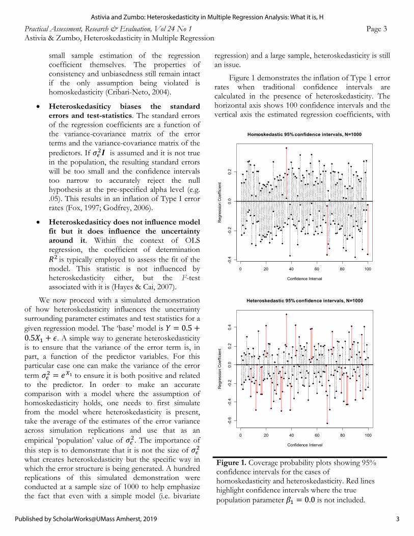
We now proceed with a simulated demonstration of how heteroskedasticity influences the uncertainty surrounding parameter estimates and test statistics for a given regression model. The ‘base’ model is 𝑌 0.50.5𝑋 𝜖. A simple way to generate heteroskedasticity is to ensure that the variance of the error term is, in part, a function of the predictor variables. For this particular case one can make the variance of the error term 𝜎 𝑒 to ensure it is both positive and related to the predictor. In order to make an accurate comparison with a model where the assumption of homoskedasticity holds, one needs to first simulate from the model where heteroskedasticity is present, take the average of the estimates of the error variance across simulation replications and use that as an empirical ‘population’ value of 𝜎 . The importance of this step is to demonstrate that it is not the size of 𝜎 what creates heteroskedasticity but the specific way in which the error structure is being generated. A hundred replications of this simulated demonstration were conducted at a sample size of 1000 to help emphasize the fact that even with a simple model (i.e. bivariate

regression) and a large sample, heteroskedasticity is still an issue.

Figure 1 demonstrates the inflation of Type 1 error rates when traditional confidence intervals are calculated in the presence of heteroskedasticity. The horizontal axis shows 100 confidence intervals and the vertical axis the estimated regression coefficients, with

Figure 1. Coverage probability plots showing 95% confidence intervals for the cases of homoskedasticity and heteroskedasticity. Red lines highlight confidence intervals where the true population parameter 𝛽 0.0 is not included.

0 20 40 60 80 100

-0.4

-0.2

0.0

0.2

Confidence Interval

Reg

ress

ion

Coe

ffic

ient

Homoskedastic 95% confidence intervals, N=1000

0 20 40 60 80 100

-0.6

-0.4

-0.2

0.0

0.2

0.4

Confidence Interval

Reg

ress

ion

Coe

ffic

ient

Heteroskedastic 95% confidence intervals, N=1000

3



Practical Assessment, Research & Evaluation, Vol 24 No 1 Page 4 Astivia & Zumbo, Heteroskedasticity in Multiple Regression the true population value for 𝛽 0.0 marked by a horizontal, bolded line. If the confidence intervals did not include the population regression coefficient, they were marked in red. For the top panel (where all the assumptions are satisfied) we can see that only 5 confidence intervals do not include the value 0.0, as expected by standard statistical theory. The bottom panel, however, shows a severe inflation of Type 1 error rates, where almost half of the calculated confidence intervals do not include the true population parameter. Since there is nothing within the standard estimation procedures that accounts for this added variability, the coverage probability is incorrect.

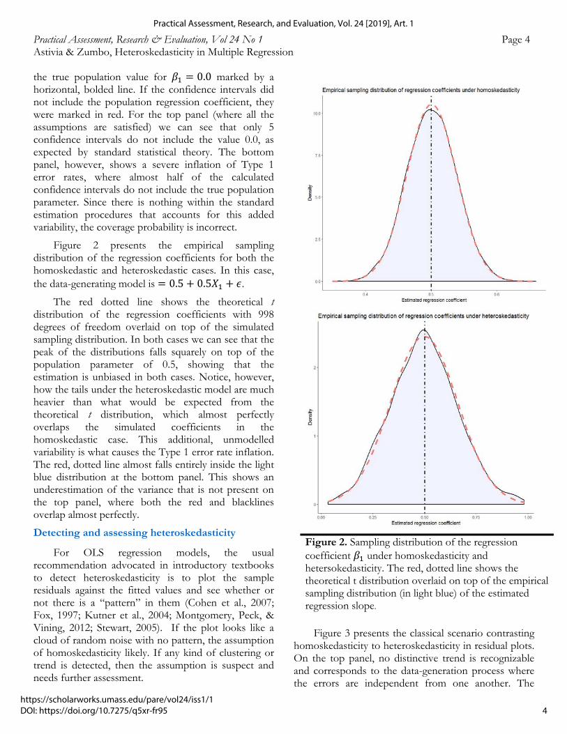
Figure 2 presents the empirical sampling distribution of the regression coefficients for both the homoskedastic and heteroskedastic cases. In this case, the data-generating model is 0.5 0.5𝑋 𝜖.

The red dotted line shows the theoretical t distribution of the regression coefficients with 998 degrees of freedom overlaid on top of the simulated sampling distribution. In both cases we can see that the peak of the distributions falls squarely on top of the population parameter of 0.5, showing that the estimation is unbiased in both cases. Notice, however, how the tails under the heteroskedastic model are much heavier than what would be expected from the theoretical t distribution, which almost perfectly overlaps the simulated coefficients in the homoskedastic case. This additional, unmodelled variability is what causes the Type 1 error rate inflation. The red, dotted line almost falls entirely inside the light blue distribution at the bottom panel. This shows an underestimation of the variance that is not present on the top panel, where both the red and blacklines overlap almost perfectly.

Detecting and assessing heteroskedasticity

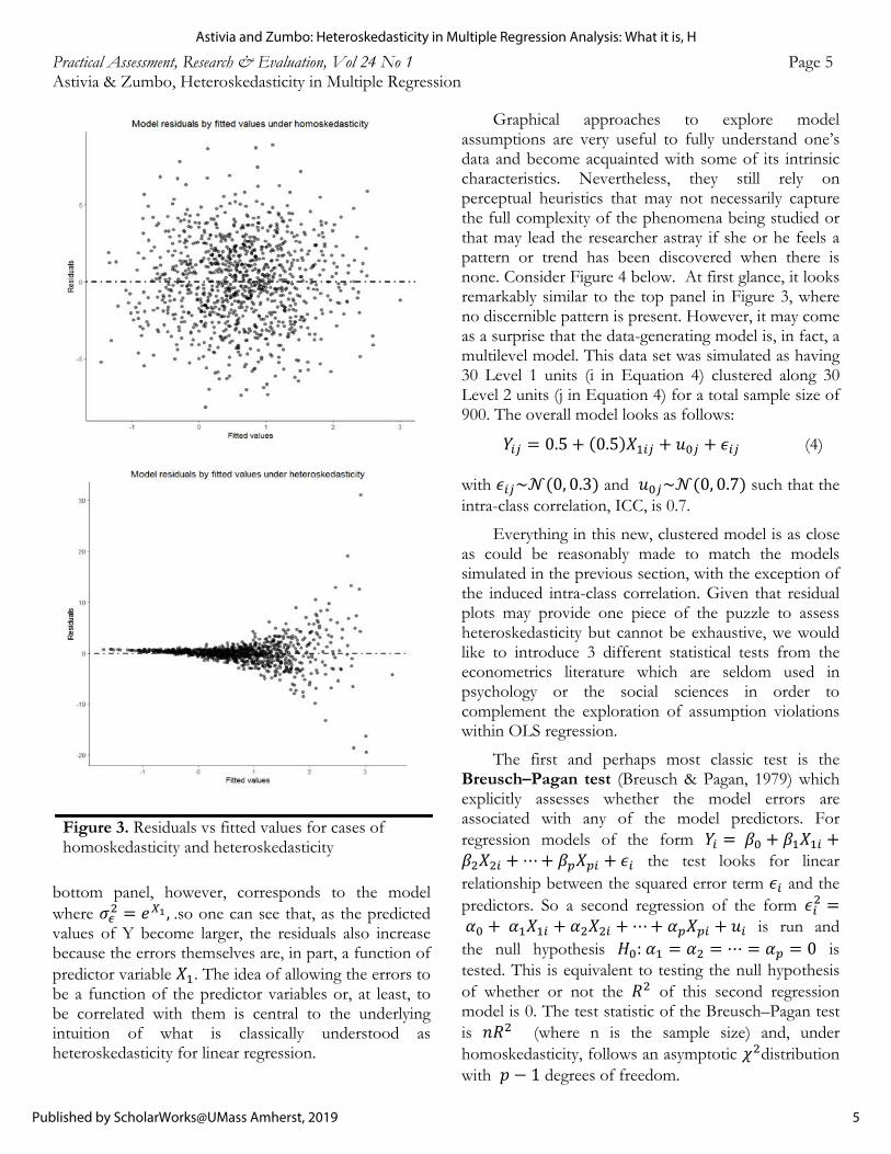
For OLS regression models, the usual recommendation advocated in introductory textbooks to detect heteroskedasticity is to plot the sample residuals against the fitted values and see whether or not there is a “pattern” in them (Cohen et al., 2007; Fox, 1997; Kutner et al., 2004; Montgomery, Peck, & Vining, 2012; Stewart, 2005). If the plot looks like a cloud of random noise with no pattern, the assumption of homoskedasticity likely. If any kind of clustering or trend is detected, then the assumption is suspect and needs further assessment.

Figure 3 presents the classical scenario contrasting homoskedasticity to heteroskedasticity in residual plots. On the top panel, no distinctive trend is recognizable and corresponds to the data-generation process where the errors are independent from one another. The

Figure 2. Sampling distribution of the regression coefficient 𝛽 under homoskedasticity and hetersokedasticity. The red, dotted line shows the theoretical t distribution overlaid on top of the empirical sampling distribution (in light blue) of the estimated regression slope.

4




bottom panel, however, corresponds to the model where 𝜎 𝑒 , .so one can see that, as the predicted values of Y become larger, the residuals also increase because the errors themselves are, in part, a function of predictor variable 𝑋 . The idea of allowing the errors to be a function of the predictor variables or, at least, to be correlated with them is central to the underlying intuition of what is classically understood as heteroskedasticity for linear regression.

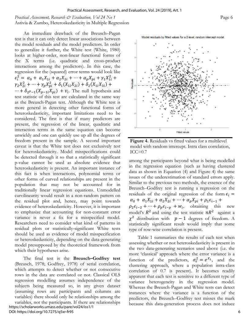
Graphical approaches to explore model assumptions are very useful to fully understand one’s data and become acquainted with some of its intrinsic characteristics. Nevertheless, they still rely on perceptual heuristics that may not necessarily capture the full complexity of the phenomena being studied or that may lead the researcher astray if she or he feels a pattern or trend has been discovered when there is none. Consider Figure 4 below. At first glance, it looks remarkably similar to the top panel in Figure 3, where no discernible pattern is present. However, it may come as a surprise that the data-generating model is, in fact, a multilevel model. This data set was simulated as having 30 Level 1 units (i in Equation 4) clustered along 30 Level 2 units (j in Equation 4) for a total sample size of 900. The overall model looks as follows:

𝑌 0.5 0.5 𝑋 𝑢 𝜖 (4)

with 𝜖 ~𝒩 0, 0.3 and 𝑢 ~𝒩 0, 0.7 such that the intra-class correlation, ICC, is 0.7.

Everything in this new, clustered model is as close as could be reasonably made to match the models simulated in the previous section, with the exception of the induced intra-class correlation. Given that residual plots may provide one piece of the puzzle to assess heteroskedasticity but cannot be exhaustive, we would like to introduce 3 different statistical tests from the econometrics literature which are seldom used in psychology or the social sciences in order to complement the exploration of assumption violations within OLS regression.

The first and perhaps most classic test is the Breusch–Pagan test (Breusch & Pagan, 1979) which explicitly assesses whether the model errors are associated with any of the model predictors. For regression models of the form 𝑌 𝛽 𝛽 𝑋𝛽 𝑋 ⋯ 𝛽 𝑋 𝜖 the test looks for linear relationship between the squared error term 𝜖 and the predictors. So a second regression of the form 𝜖 𝛼 𝛼 𝑋 𝛼 𝑋 ⋯ 𝛼 𝑋 𝑢 is run and the null hypothesis 𝐻 : 𝛼 𝛼 ⋯ 𝛼 0 is tested. This is equivalent to testing the null hypothesis of whether or not the 𝑅 of this second regression model is 0. The test statistic of the Breusch–Pagan test is 𝑛𝑅 (where n is the sample size) and, under homoskedasticity, follows an asymptotic 𝜒 distribution with 𝑝 1 degrees of freedom.

Figure 3. Residuals vs fitted values for cases of homoskedasticity and heteroskedasticity

5




An immediate drawback of the Breusch–Pagan test is that it can only detect linear associations between the model residuals and the model predictors. In order to generalize it further, the White test (White, 1980) looks at higher-order, non-linear functional forms of the X terms (i.e. quadratic and cross-product interactions among the predictors). In this case, the regression for the (squared) error terms would look like 𝜖 𝛼 𝛼 𝑋 𝛼 𝑋 ⋯ 𝛼 𝑋 𝛾 𝑋𝛾 𝑋 ⋯ 𝛾 𝑋 𝛿 𝑋 𝑋 𝛿 𝑋 𝑋⋯ 𝛿 𝑋 𝑋 𝑣 . The null hypothesis and test statistic of this test are calculated in the same way as the Breusch-Pagan test. Although the White test is more general in detecting other functional forms of heteroskedasticity, important limitations need to be considered. The first is that if many predictors are present, the regression of the linear, quadratic and interaction terms in the same equation can become unwieldy and one can quickly use up all the degrees of freedom present in the sample. A second important caveat is that the White test does not exclusively test for heteroskedasticity. Model misspecifications could be detected through it so that a statistically significant p-value cannot be used as absolute evidence that heteroskedasticity is present. An important instance of this fact is when interactions, polynomial terms or other forms of curved relationships are present in the population that may not be accounted for in traditionally linear regression equations. Unmodelled curvilinearity would result in a non-random pattern on the residual plot and, hence, may point towards evidence of heteroskedasticity. However, it is important to emphasize that accounting for non-constant error variance is never a fix for a misspecified model. Researchers need to consider what kind of patterns in residual plots or statistically-significant White tests should be used as evidence of model misspecification or heteroskedasticity, depending on the data-generating model presupposed by the theoretical framework from which their hypotheses arise.

The final test is the Breusch–Godfrey test (Breusch, 1978; Godfrey, 1978) of serial correlation, which attempts to detect whether or not consecutive rows in the data are correlated or not. Classical OLS regression modelling assumes independence of the subjects being measured so, in any given dataset (assuming rows are participants and columns are variables) there should only be relationships among the variables, not the participants. If there are relationships

among the participants beyond what is being modelled in the regression equation (such as having clustered data as shown in Equation (4) and Figure 4) the same issues of the underestimation of standard errors apply. Similar to the previous two methods, the essence of the Breusch–Godfrey test is running a regression on the residuals of the original regression of the form 𝜖 𝛼 𝛼 𝑋 𝛼 𝑋 ⋯ 𝛼 𝑋 𝜌 𝜖𝜌 𝜖 ⋯ 𝜌 𝜖 𝑤 , obtaining this new model’s 𝑅 and using the test statistic 𝑛𝑅 against a 𝜒 distribution with 𝑝 1 degrees of freedom. A statistically significant result would imply that some type of row-wise correlation is present.

Table 1 summarizes the results of each test when assessing whether or not heteroskedasticity is present in the two data-generating scenarios used above (i.e. the more ‘classical’ approach where the error variance is a function of the predictors, 𝜎 𝑒 , and the clustering approach, where a population intra-class correlation of 0.7 is present). It becomes readily apparent that each test is sensitive to a different type of variance heterogeneity in the regression model. Whereas the Breusch-Pagan and White tests can detect instances where the variance is a function of the predictors, the Breusch–Godfrey test misses the mark because this data-generation process does not induce

Figure 4. Residuals vs fitted values for a multilevel model with random intercept. Intra class correlation, ICC=0.7

6



Practical Assessment, Research & Evaluation, Vol 24 No 1 Page 7 Astivia & Zumbo, Heteroskedasticity in Multiple Regression any relationship between the simulated participants (i.e. the rows), only the variables (i.e. the columns).

Table 1. P-values (p) for each type of the different tests assessing two types of heteroskedasticity

Heteroskedasticity Breusch‐Pagan White

Breusch‐Godfrey

Classic <.0001 <.0001 0.1923

Clustering 0.4784 0.5883 <.0001

When one encounters clustering, however, the situation reverses and now the Breusch–Godfrey test is the only one that can successfully detect a violation of the constant variance assumption. Clustering induces variability in the model above and beyond what can be assumed by the predictors, therefore, neither the Breusch-Pagan nor the White test are sensitive to it. It is important to point out, however, that for the Breusch–Godfrey test to detect heteroskedasticity, the rows of the dataset need to be ordered such that continuous rows are members of the same cluster. If the rows were scrambled, heteroskedasticity would still be present, but the former test would be unable to detect it. Diagnosing heteroskedasticity is not a trivial matter because whether one relies on graphical devices or formal statistical approaches, a model generating the differences in variances is always assumed and if this model does not correspond to what is being tested, one may incorrectly assume that homoskedasticity is present when it is not.

Fixing heteroskedasticity Pt. I: Heteroskedastic-consistent standard errors

Traditionally, the first (and perhaps only) approach that most researchers within psychology or the social sciences are familiar with to handle heteroskedasticity is data transformation (Osborne, 2005; Rosopa, Schaffer, & Schroeder, 2013). The logarithmic transformation tends to be popular along with other “variance stabilizing” ones such as the square root. Transformations, unfortunately, carry a certain degree of arbitrariness in terms of which one to choose rather than others. They can also fundamentally change the meaning of the variables (and the regression model itself) so that the interpretation of parameter estimates is now contingent on the new scaling induced by the transformation (Mueller, 1949). And, finally, it is not difficult to find oneself in situations where the transformations have limited to no effect, rendering invalid the only method that most researchers are

familiar with to tackle this issue. We will now present two distinct, statistically-principled approaches to accommodate for non-constant variance that, with very little input, can fundamentally yield more proper inferences and change very little in the way of analysis an interpretation of regression models.

The first approach are heteroskedastic-consistent standard errors (Eicker, 1967; Huber, 1967; White, 1980) also known as White standard errors, Huber-White standard errors, robust standard errors, sandwich estimators, etc. which essentially recognize the presence of non-constant variance and offer an alternative approach to estimating the variance of the sample regression coefficients.

Recall from Section 1, Equation (3) that if the more general form of heteroskedasticity is assumed, the variance-covariance matrix of the regression model errors follows the form:

𝑉𝑎𝑟 𝜖 𝔼 𝜖𝜖

⎣⎢⎢⎢⎢⎡

𝜎 , 𝜎 , ⋯ 𝜎 , 𝜎 ,

𝜎 , 𝜎 , ⋯ 𝜎 , 𝜎 ,

⋮𝜎 ,

𝜎 ,

⋮𝜎 ,

𝜎 ,

𝜎 , ⋮ ⋮𝜎 ,

⋯⋱ 𝜎 ,

𝜎 , 𝜎 , ⎦⎥⎥⎥⎥⎤

𝛀

Call this matrix 𝛀. For a traditional OLS regression model expressed in vector and matrix form 𝐲 𝐗𝛃 𝛜 the variance of the estimated regression coefficients is simply 𝑉𝑎𝑟 𝛽 𝜎 𝐗 𝐗 with 𝜎 defined as above. When heteroskedasticity is present, the variance of the estimated regression coefficients becomes:

𝑉𝑎𝑟 𝛽 𝐗 𝐗 𝐗 𝛀𝐗 𝐗 𝐗 (5)

Notice that if 𝛀 𝜎 𝑰 like in Equation (1), then the expression for Equation (5) reduces back to 𝑉𝑎𝑟 𝛽 𝜎 𝐗 𝐗 . It now becomes apparent that to obtain the proper standard errors to account for non-constant variance, the matrix 𝛀 needs to play a role in their calculation.

The rationale behind how to create these new standard errors goes as follows. Just as with any given sample, all we have is an estimate 𝛀 that will be needed to obtain these new uncertainties. Recall that the diagonal of the matrix expressed in 𝜎 𝐗 𝐗 provides the central elements to obtain the standard errors of the regression coefficients. All that is needed is to take its square root and weigh it by the inverse of the

7



Practical Assessment, Research & Evaluation, Vol 24 No 1 Page 8 Astivia & Zumbo, Heteroskedasticity in Multiple Regression sample size. Now, since 𝛀 originates from the residuals of the regression model (as estimates of the population regression errors), the conceptual idea behind heteroskedastic-consistent standard errors is to use the variance of each sample residual 𝑟 to estimate the variance of the population errors 𝜖 (i.e. the diagonal elements of 𝛀). Now, because there is only one residual 𝑟 per person, per sample, this is a one-sample estimate, so 𝑉𝑎𝑟 𝜖̂ 𝑟 0 /1 𝑟 (recall that, by assumption, the mean of the residuals is 0). Therefore, let 𝛀 𝑑𝑖𝑎𝑔 𝑟 and back-substituting it in Equation (5) implies

𝑉𝑎𝑟 𝛽 𝐗 𝐗 𝐗 𝑑𝑖𝑎𝑔 𝑟 𝐗 𝐗 𝐗 (6)

Equation (6) is the oldest and most widely used form of heteroskedastic-consistent standard errors and has been shown in Huber (1967) and White (1980) to be a consistent estimator of 𝑉𝑎𝑟 𝛽 even if the specific form of heteroskedasticity is not known. There are other versions of this standard error that offer alternative adjustments which perform better for small sample sizes, but they all follow a similar pattern to what is shown in Equation (6). The key issue is to obtain a better estimate of 𝛀 so that the new standard errors yield the correct Type I error rate. MacKinnon and White (1985) offer a comprehensive list of these alternative approaches as well as recommendations of which ones to use under which circumstances.

Figure 5 presents a simulation of 100 heteroskedastic-consistent confidence intervals obtained from applying Equation (6) to the two different types of heteroskedasticity highlighted in this article: the ‘classic’ heteroskedasticity, where the variance of the error terms is a function of a predictor variable (i.e. 𝜎 𝑒 ) and the ‘clustered’ heteroskedasticity, where a population ICC of 0.7 is present in the data. The latter case would mimic the real-life scenario of a researcher either ignoring or being unaware that the data is structured hierarchically and analyzing it as if it were a single-level model as opposed to a two-level, multilevel model. Compare Figure 5 to the bottom panel of Figure 1. It becomes immediately apparent that heteroskedastic-consistent standard errors (and the confidence intervals derived from them) perform considerably better at preserving Type I error rate when compared to the naïve approach of ignoring non-constant error variance. Moreover, it is important to highlight that, in spite of the different

heteroskedastic-generation processes, the robust correction was able to adjust for them and yield valid inferences without necessarily having to assume any specific functional form for them. This stems from the fact that all the information regarding the variability of the parameter estimates is contained within both the design matrix X' X and the matrix Ω defined above.

Figure 5. Coverage probability plots showing heteroskedastic-consistent, 95% confidence intervals for both classical (i.e. 𝜎 𝑒 and clustered (i.e. ICC=0.7) heteroskedasticity. Pink lines highlight confidence intervals where the true population parameter 𝛽 0.5 is not included.

0 20 40 60 80 100

0.0

0.2

0.4

0.6

0.8

1.0

Confidence Interval

Reg

ress

ion

Coe

ffic

ient

Robust 95% confidence intervals for classicheteroskedasticity

0 20 40 60 80 100

0.35

0.40

0.45

0.50

0.55

0.60

0.65

Confidence Interval

Reg

ress

ion

Coe

ffic

ient

Robust 95% confidence intervals for clusteredheteroskedasticity

8




If one operates on these two matrices directly, it is possible to obtain asymptotically efficient corrections to the standard errors without the need for further assumptions. Other alternative approaches such as the use of multilevel models do require the researcher to know in advance something about where the variability is coming from like a random effect for the intercept, a random effect for a slope, for an interaction, etc. (McNeish et al., 2017). If the model is misspecified by assuming a certain random effect structure for the data that is not true in the population, the inferences will still be suspect. This is perhaps one of the reasons of why popular software like HLM provides default output not correctly specified. Ultimately, whether one opts to analyze the data using robust standard errors or an HLM model depends on the research hypothesis and whether or not the additional sources of variation are relevant to the question at hand or are nuisance parameters that need to be corrected for.

Fixing heteroskedasticity Pt II: The ‘wild bootstrap’

Computer-intensive approaches to data analysis and inference have gained tremendous popularity in recent decades given both advances in modern statistical theory and the accessibility to cheap computer power. Among these approaches, the bootstrap procedure is perhaps the most popular one, since it allows for proper inferences without the need of overly strict assumptions. This is one of the reasons for why it has become one of the ‘go-to’ strategies to calculate confidence intervals and p-values whenever issues such as small sample sizes or violations of parametric assumptions are present. A good introduction to the method of the bootstrap can be found in Mooney, Duval, and Duvall (1993).

A very important aspect to consider when using the bootstrap is how to re-sample the data. For simple procedures such as calculating a confidence interval for the sample mean, the usual random sampling-with-replacement approach is sufficient. For more complicated models, what gets and does not get re-sampled has a very big influence on whether or not the resulting confidence intervals and p-values are correct. When heteroskedasticity is present this becomes a crucial issue because a regular random sampling-with replacing approach would naturally break the heteroskedasticity of the data, imposing homoskedasticity in the bootstrapped samples and making the bootstrapped confidence intervals too

narrow (MacKinnon, 2006). We would essentially find ourselves again in a situation similar to the bottom panel of Figure 1. In order to address the issue of generating multiple bootstrapped samples that still preserve the heteroskedastic properties of the residuals, an alternative procedure known as the wild bootstrap has been proposed in econometrics (Davidson & Flachaire, 2008; Wu, 1986).

There is more than one way to bootstrap linear regression models. Residual bootstrap tends to be recommended on the literature (c.f.(Cameron, Gelbach, & Miller, 2008; Hardle & Mammen, 1993; MacKinnon, 2006) and proceeds with the following steps:

(1) Fit the regular regression model 𝑌 𝑏𝑏 𝑋 +𝑏 𝑋 ⋯ 𝑏 𝑋 .

(2) Calculate the residuals 𝑟 𝑌 𝑌

(3) Create bootstrapped samples of the residuals 𝑟 and add those back to 𝑌 so that the new bootstrapped 𝑌 is now 𝑌 𝑌 𝑟

(4) Regress every new 𝑌 on the predictors 𝑋 , 𝑋 , … , 𝑋 and save the regression coefficients

each time.

Notice how, in accordance to the assumptions of fixed-effects regression, the variability comes exclusively from the only random part of the model, the residuals. Every new 𝑌 exists only because new samples (with replacement) of residuals 𝑟 are created at every iteration. Everything else (the matrix of predictors 𝐗 and the predicted 𝑌 ) are exactly the same as what was estimated originally in Step 1. From this brief summary we can readily see why this strategy would not be ideal for models that exhibit heteroskedasticty. The process of randomly sampling the residuals 𝑟 would break any association with the matrix of predictors 𝐗 or among the residuals themselves, which are both intrinsic to what it means for an OLS regression model to be heteroskedastic.

Although the details of the wild bootstrap are beyond the scope of this introductory overview (interested readers can consult Davidson and Flachaire, 2008), the solution it presents is remarkably elegant and relatively straightforward to understand. All it requires is to assume that the regression model is expressed as

𝑌 𝛽 𝛽 𝑋 𝛽 𝑋 ⋯ 𝛽 𝑋 𝑓 𝜖 𝑢

9




where 𝑓 𝜖 is a transformation of the residuals and the weights 𝑢 have a mean of zero. By choosing suitable transformation functions 𝑓 ∙ and weights 𝑢 , one can proceed with the usual four steps for residual bootstrapping and obtain inferences that still account for the heteroskedasticity of the data.

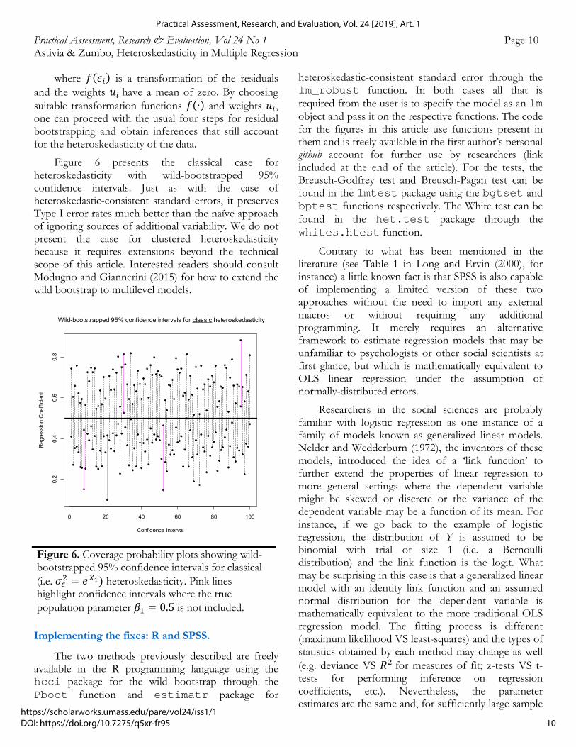
Figure 6 presents the classical case for heteroskedasticity with wild-bootstrapped 95% confidence intervals. Just as with the case of heteroskedastic-consistent standard errors, it preserves Type I error rates much better than the naïve approach of ignoring sources of additional variability. We do not present the case for clustered heteroskedasticity because it requires extensions beyond the technical scope of this article. Interested readers should consult Modugno and Giannerini (2015) for how to extend the wild bootstrap to multilevel models.

Implementing the fixes: R and SPSS.

The two methods previously described are freely available in the R programming language using the hcci package for the wild bootstrap through the Pboot function and estimatr package for

heteroskedastic-consistent standard error through the lm_robust function. In both cases all that is required from the user is to specify the model as an lm object and pass it on the respective functions. The code for the figures in this article use functions present in them and is freely available in the first author’s personal github account for further use by researchers (link included at the end of the article). For the tests, the Breusch-Godfrey test and Breusch-Pagan test can be found in the lmtest package using the bgtset and bptest functions respectively. The White test can be found in the het.test package through the whites.htest function.

Contrary to what has been mentioned in the literature (see Table 1 in Long and Ervin (2000), for instance) a little known fact is that SPSS is also capable of implementing a limited version of these two approaches without the need to import any external macros or without requiring any additional programming. It merely requires an alternative framework to estimate regression models that may be unfamiliar to psychologists or other social scientists at first glance, but which is mathematically equivalent to OLS linear regression under the assumption of normally-distributed errors.

Researchers in the social sciences are probably familiar with logistic regression as one instance of a family of models known as generalized linear models. Nelder and Wedderburn (1972), the inventors of these models, introduced the idea of a ‘link function’ to further extend the properties of linear regression to more general settings where the dependent variable might be skewed or discrete or the variance of the dependent variable may be a function of its mean. For instance, if we go back to the example of logistic regression, the distribution of Y is assumed to be binomial with trial of size 1 (i.e. a Bernoulli distribution) and the link function is the logit. What may be surprising in this case is that a generalized linear model with an identity link function and an assumed normal distribution for the dependent variable is mathematically equivalent to the more traditional OLS regression model. The fitting process is different (maximum likelihood VS least-squares) and the types of statistics obtained by each method may change as well (e.g. deviance VS 𝑅 for measures of fit; z-tests VS t-tests for performing inference on regression coefficients, etc.). Nevertheless, the parameter estimates are the same and, for sufficiently large sample

Figure 6. Coverage probability plots showing wild-bootstrapped 95% confidence intervals for classical (i.e. 𝜎 𝑒 heteroskedasticity. Pink lines highlight confidence intervals where the true population parameter 𝛽 0.5 is not included.

0 20 40 60 80 100

0.2

0.4

0.6

0.8

Confidence Interval

Re

gres

sion

Coe

ffic

ient

Wild-bootstrapped 95% confidence intervals for classicheteroskedasticity

10



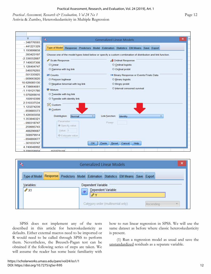
Practical Assessment, Research & Evaluation, Vol 24 No 1 Page 11 Astivia & Zumbo, Heteroskedasticity in Multiple Regression sizes, the inferences will also be the same. SPSS does not have an option to obtain heteroskedastic-consistent standard errors in its linear regression drop-down menu, but it does offer the option in its generalized linear model drop-down menu so that, by fitting a regression through maximum likelihood, we can request the option to calculate the same robust standard errors used in this article. A tutorial with simulated data will be presented here to guide the reader through the steps to obtain heteroskedastic-consistent standard errors. We will use a sample dataset where the data-generating regression model is 𝑌0.5 0.5 𝑋 𝜖 In this model, 𝑋 ~𝑁 0,1 , 𝜖~𝑁 0, 𝑒 and the sample size is 1000.

(1) Once the dataset is loaded, go to the “Generalized Linear Models” sub-menu and click on it.

(2) Under the “Type of Model” tab ensure that the ‘custom’ option is enabled and select ‘Normal’ for the distribution and ‘Identity’ for the link function.

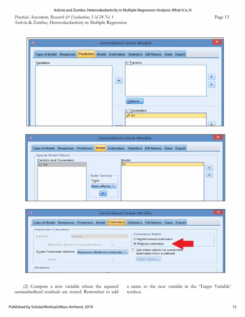
(3) The next steps should be familiar to SPSS users In the ‘Response’ tab one selects the dependent variable…in the ‘Predictors’ tab one chooses the independent variables or ‘Covariates’ in this case (there is only one for the present example) and the ‘Model’ tab helps the user specify main-effects-only models or main effects with interactions. We are specifying “Main

effects” because there is only one predictor with no interactions.

(4) The final (and most important) step is to make sure that under the ‘Estimation’ tab the ‘Robust estimator’ option for the Covariance Matrix is selected. This step ensures that heteroskedastic-consistent standard errors are calculated as part of the regression output .

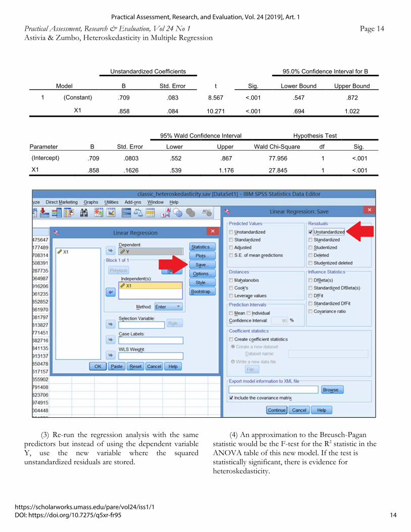
Below we compare the output of the coefficients table from the standard ‘Linear regression’ menu (top table) to the output from the new approach described here, where the model is fit as a generalized linear model with a normal distribution as a response variable and the identity link function (bottom table):

In both cases, the parameter estimates are exactly the same 𝑏 0.709, 𝑏 0.858 but the standard errors are different. The heteroskedastic-consistent standard error for the slope is .1626 whereas the regular one (assuming homoskedasticity) is .0803. The standard error estimated using the new, robust approach is almost twice the size of the one shown using the common linear regression approach. This reflects the fact that more uncertainty is present in the analysis due to the higher levels of variability that heteroskedasticity induces. The Wald confidence intervals also mirror this because they are wider than the t-distribution ones from the regular regression approach.

11




SPSS does not implement any of the tests described in this article for heteroskedasticity as defaults. Either external macros need to be imported or R would need to be called through SPSS to perform them. Nevertheless, the Breusch-Pagan test can be obtained if the following series of steps are taken. We will assume the reader has some basic familiarity with

how to run linear regression in SPSS. We will use the same dataset as before where classic heteroskedasticity is present.

(1) Run a regression model as usual and save the unstandardized residuals as a separate variable.

12




(2) Compute a new variable where the squared unstandardized residuals are stored. Remember to add

a name to the new variable in the ‘Target Variable’ textbox.

13




(3) Re-run the regression analysis with the same predictors but instead of using the dependent variable Y, use the new variable where the squared unstandardized residuals are stored.

(4) An approximation to the Breusch-Pagan statistic would be the F-test for the R2 statistic in the ANOVA table of this new model. If the test is statistically significant, there is evidence for heteroskedasticity.

Model

Unstandardized Coefficients

t Sig.

95.0% Confidence Interval for B

B Std. Error Lower Bound Upper Bound

1 (Constant) .709 .083 8.567 <.001 .547 .872

X1 .858 .084 10.271 <.001 .694 1.022

Parameter B Std. Error

95% Wald Confidence Interval Hypothesis Test

Lower Upper Wald Chi-Square df Sig.

(Intercept) .709 .0803 .552 .867 77.956 1 <.001

X1 .858 .1626 .539 1.176 27.845 1 <.001

14




References 1. Breusch, T. S. (1978). Testing for autocorrelation in

dynamic linear models. Australian Economic Papers, 17, 334-355. doi:10.1111/j.1467-8454.1978.tb00635.x

2. Breusch, T. S., & Pagan, A. R. (1979). A simple test for heteroscedasticity and random coefficient variation. Econometrica: Journal of the Econometric Society, 1287-1294. doi:10.2307/1911963

3. Cameron, A. C., Gelbach, J. B., & Miller, D. L. (2008). Bootstrap-based improvements for inference with clustered errors. The Review of Economics and Statistics, 90, 414-427. doi:10.1162/rest.90.3.414

4. Cohen, P., West, S. G., & Aiken, L. S. (2007). Applied multiple regression/correlation analysis for the behavioral sciences. Mahwah, NJ: Erlbaum.

5. Cribari-Neto, F. (2004). Asymptotic inference under heteroskedasticity of unknown form. Computational Statistics & Data Analysis, 45, 215-233. doi:10.1016/S0167-9473(02)00366-3

6. Davidson, R., & Flachaire, E. (2008). The wild bootstrap, tamed at last. Journal of Econometrics, 146, 162-169. doi:10.1016/j.jeconom.2008.08.003

7. Eicker, F. (1967). Limit theorems for regressions with unequal and dependent errors. Paper presented at the Proceedings of the fifth Berkeley symposium on mathematical statistics and probability.

8. Field, A. (2009). Discovering Statistics Using SPSS (3rd ed.). London, UK: Sage.

9. Fox, J. (1997). Applied regression analysis, linear models, and related methods. Thousand Oaks, CA: Sage Publications, Inc.

10. Godfrey, L. (1978). Testing against general autoregressive and moving average error models when the regressors include lagged dependent variables. Econometrica: Journal of the Econometric Society, 1293-1301. doi:10.2307/1913829

11. Godfrey, L. (2006). Tests for regression models with heteroskedasticity of unknown form. Computational Statistics & Data Analysis, 50, 2715-2733. doi:10.1016/j.csda.2005.04.004

12. Hardle, W., & Mammen, E. (1993). Comparing nonparametric versus parametric regression fits. The Annals of Statistics, 21, 1926-1947. doi:10.1214/aos/1176349403

13. Hayes, A. F., & Cai, L. (2007). Using heteroskedasticity-consistent standard error estimators in OLS regression:

An introduction and software implementation. Behavior Research Methods, 39, 709-722. doi:10.3758/BF03192961

14. Huber, P. J. (1967). The behavior of maximum likelihood estimates under nonstandard conditions. Paper presented at the Proceedings of the fifth Berkeley symposium on mathematical statistics and probability.

15. Kutner, M. H., Nachtsheim, C., & Neter, J. (2004). Applied linear regression models. Homewood, IL: McGraw-Hill/Irwin.

16. Long, J. S., & Ervin, L. H. (2000). Using heteroscedasticity consistent standard errors in the linear regression model. The American Statistician, 54, 217-224. doi:10.1080/00031305.2000.10474549

17. MacKinnon, J. G. (2006). Bootstrap methods in econometrics. Economic Record, 82, S2-S18. doi:10.1111/j.1475-4932.2006.00328.x

18. MacKinnon, J. G., & White, H. (1985). Some heteroskedasticity-consistent covariance matrix estimators with improved finite sample properties. Journal of Econometrics, 29, 305-325. doi:10.1016/0304-4076(85)90158-7

19. McNeish, D., Stapleton, L. M., & Silverman, R. D. (2017). On the unnecessary ubiquity of hierarchical linear modeling. Psychological Methods, 22, 114-140. doi:10.1037/met0000078

20. Modugno, L., & Giannerini, S. (2015). The wild bootstrap for multilevel models. Communications in Statistics-Theory and Methods, 44, 4812-4825. doi:10.1080/03610926.2013.802807

21. Montgomery, D. C., Peck, E. A., & Vining, G. G. (2012). Introduction to linear regression analysis (Vol. 821). Hoboken, NJ: John Wiley & Sons.

22. Mooney, C. Z., Duval, R. D., & Duvall, R. (1993). Bootstrapping: A nonparametric approach to statistical inference. Newbury Park, CA: Sage.

23. Mueller, C. G. (1949). Numerical transformations in the analysis of experimental data. Psychological Bulletin, 46, 198-223. doi:10.1037/h0056381

24. Nelder, J. A., & Wedderburn, R. W. M. (1972). Generalized Linear Models. Journal of the Royal Statistical Society. Series A (General), 135, 370-384. doi:10.2307/2344614

25. Osborne, J. (2005). Notes on the use of data transformations. Practical Assessment, Research and Evaluation, 9, 42-50.

15



Practical Assessment, Research & Evaluation, Vol 24 No 1 Page 16 Astivia & Zumbo, Heteroskedasticity in Multiple Regression 26. Rosopa, P. J., Schaffer, M. M., & Schroeder, A. N.

(2013). Managing heteroscedasticity in general linear models. Psychological Methods, 18, 335-351. doi:10.1037/a0032553

27. Stewart, K. G. (2005). Introduction to applied econometrics. Cole Belmont, CA: Thomson Brooks.

28. White, H. (1980). A heteroskedasticity-consistent covariance matrix estimator and a direct test for

heteroskedasticity. Econometrica: Journal of the Econometric Society, 817-838. doi:10.2307/1912934

29. Wu, C.-F. J. (1986). Jackknife, bootstrap and other resampling methods in regression analysis. the Annals of Statistics, 14, 1261-1295. doi:10.1214/aos/1176350142

Note

R code for figures and analysis can be found in https://raw.githubusercontent.com/OscarOlvera/R-code-for-publications/master/heteroskedasticity The SPSS data and code can be found in https://pareonline.net/sup/v24n1.zip

Citation:

Astivia, Oscar L. Olvera and Zumbo, Bruno D. (2019). Heteroskedasticity in Multiple Regression Analysis: What it is, How to Detect it and How to Solve it with Applications in R and SPSS. Practical Assessment, Research & Evaluation, 24(1). Available online: http://pareonline.net/getvn.asp?v=24&n=1

Corresponding Authors

Oscar L. Olvera Astivia School of Population and Public Health The University of British Columbia 2206 East Mall Vancouver, British Columbia V6T 1Z3, Canada email: oolvera[at]mail.ubc.ca Bruno D. Zumbo Paragon UBC Professor of Psychometrics & Measurement Measurement, Evaluation & Research Methodology Program The University of British Columbia Scarfe Building, 2125 Main Mall Vancouver, British Columbia V6T 1Z4, Canada email: bruno.zumbo [at] ubc.ca

16



Heteroskedasticity in Multiple Regression Analysis: What ...

Documents

Transcript of Heteroskedasticity in Multiple Regression Analysis: What ...