NBER WORKING PAPER SERIES

HETEROGENEOUS INFORMATION ARRIVALSAND RETURN VOLATILITY DYNAMICS :UNCOVERING THE LONG-RUN IN HIGH

FREQUENCY RETURNS

Torben G. AndersenTim Bollerslev

Working Paper 5752

NATIONAL BUREAU OF ECONOMIC RESEARCH1050 Massachusetts Avenue

Cambridge, MA 02138September 1996

We gratefully acknowledge the financial support provided by a research grant from the Institute forQuantitative Research in Finance (the Q-Group). We would also like to thank Olsen and Associatesfor providing the intradaily exchange rates and Reuter’s news tape analyzed in the paper. This paperis part of NBER’s research program in Asset Pricing. Any opinions expressed are those of theauthors and not those of the National Bureau of Economic Research.

O 1996 by Torben G, Andersen and Tim Bollerslev. All rights reserved. Short sections of text, notto exceed two paragraphs, may be quoted without explicit permission provided that full credit,including O notice, is given to the source.

NBER Working Paper 5752September 1996

HETEROGENEOUS INFORMATION ARRIVALSAND RETURN VOLATILITY DYNAMICS :UNCOVERING THE LONG-RUN IN HIGH

FREQUENCY RETURNS

ABSTRACT

Recent empirical evidence suggests that the long-run dependence in financial market

volatility is best characterized by a slowly mean-reverting fractionally integrated process. At the

same time, much shorter-lived volatility dependencies are typically observed with high-frequency

intradaily returns. This paper draws on the information arrival, or mixture-of-distributions

hypothesis interpretation of the latent volatility process in rationalizing this behavior. By

interpreting the overall volatility as the manifestation of numerous heterogeneous information

arrivals, sudden bursts of volatility typically will have both short-run and long-run components.

Over intradaily frequencies, the short-run decay stands out most clearly, while the impact of the

highly persistent processes will be dominant over longer horizons. These ideas are confirmed by our

empirical analysis of a one-year time series of intradaily five-minute Deutschemark - U.S. Dollar

returns. Whereas traditional time series based measures for the temporal dependencies in the

absolute returns give rise to very conflicting results across different intradaily sampling frequencies,

the corresponding semiparametric estimates for the order of fractional integration remain remarkably

stable. Similarly, the autocorrelogram for the low-pass filtered absolute returns, obtained by

annihilating periods in excess of one day, exhibit a striking hyperbolic rate of decay.

Torben G, Andersen Tim BollerslevDepartment of Finance Department of EconomicsJ.L. Kellogg Graduate School of Management Rouss HallNorthwestern University University of Virginia2003 Sheridan Road Charlottesville, VA 22903Evanston, IL 60208 and NBERt-andersen@nwu.edu bollerslev@virginia. edu

“Among tbe most puzzling issues is the behavior of volatility, While the general properties of volatilityremain elusive, perhaps the most intriguing feature revealed by empirical work on volatili~ is its longpemistence. Such behavior has sparked a search, almost akin to that for the Holy Grail, for the perfectGARCH model, but the underlying question of why such volatility persistence endures remains unanswered.We conjecture that the ability to analyze higher frequency data may be particularly useful in pursuing thisissue, ” (Goodhart and O’Hara (1996))

1. INTRODUCTION

A large body of literature seeking to characterize the long-run dependencies in the interdaily volatility

of speculative returns has emerged over the past decade. 1 More recently, there has been an

explosicm in the amount of empirical research devoted to the determination of high frequency

intradaily return volatility dynamics. 2 Unfortunately, the empirical estimates pertaining to the degree

of volatili~ persistence reported in these two strands of the literature often appear at odds with one

another. While studies using daily or lower frequency returns generally point to a very high degree

of intertemporal volatility dependence, the estimated half-lives of most identifiable intraday volatili~

shocks seem rather low, with any noticeable effects on the overall volatility level typically gone in

a matter of hours or less. The analysis in the present paper provides a theoretical justification for

these seemingly contradictory findings. By interpreting the overall volatility as the aggregation of

numerous independent volatility components, each endowed with their own dependence structure,

we show how the aggregate volatility process may inherit the kind of long-run dependencies

associated with long-memory, or fractiomlly integrated processes. Consequently, the

autocorrelations for more distantly spaced absolute or squared returns, should exhibit a slow

hyperbolic rate of decay, independent of the sampling frequency.

This mixture-of-distributions hypothesis interpretation of market volatility as resulting from

the aggregation of numerous components type processes apply equally well across most financial

markets and instruments. However, for concreteness the empirical analysis in the paper is focussed

on the foreign exchange market, and a one-year time span of 5-minute Deutschemark - U.S. Dollar

(DM-$) returns. Consistent with the notion of an underlying component structure, we find that the

dynamic response of the absolute 5-minute foreign exchange returns varies systematically across

‘ See Bo[lerslev, Chou and Kroner (1992) for a survey of this literature using ARCH type models.

2 For a recent survey of this literature see Goodhart and O’Hara (1996).

1

some of the most important and readily identifiable macroeconomic announcements. Furthermore,

the volatility process is shown to exhibit the kind of long-memory dependencies implied by the

theoretical aggregation of such multiple individual component processes. This interpretation of

volatility is further underscored by the fact that the corresponding estimates for the fractional orders

of integration for the absolute returns remain remarkably stable across all of the intradaily sampling

frequencies.

Although these empirical findings consistently point to the presence of long-memory, the

pronounced intradaily volatili~ patterns, known to exist in most financial markets, severely

complicate any further direct analysis of the long-run volatility dependencies. However, by low-pass

filtering the absolute intradaily returns, thus annihilating any cyclical behavior with a periodicity of

less than one day, we demonstrate how it is possible to uncover the salient long-run volatility

dynamics using standard correlation based measures. Specifically, whereas the autocorrelogram for

the raw absolute intradaily returns periodically turn negative, the autocorrelograrn for the low-pass

filtered absolute intradaily returns display a striking hyperbolic rate of decay. Consequently, these

filtered returns constitute an ideal basis for more comprehensive analyses of the important volatili~

determinants, as illustrated by our estimation of the amouncement effects associated with the

regularly scheduled release of different macroeconomic “news”.

The plan for the remainder of the paper is as follows. Section 2 briefly reviews some of the

existing literature on the intradaily dependencies in the foreign exchange market. This section also

presents preliminary estimation results for specific announcement effects that point to the existence

of multiple volatility components and long-run dependencies. The mixture-of-distributions hypothesis

and the temporal aggregation argument are presented in section 3, where we show that, under

suitable assumptions concerning the underlying component structure, the spectrum for the overall

volatility process implies an eventual slow hyperbolic rate of decay in the autocorrelations for the

absolute returns, irrespective of the sampling frequency. The theoretical developments are validated

by the empirical analysis in section 4, which reports the results obtained from two alternative

spectral-domain estimators for the degree of fractional integration in the volatility process across a

range of different intradaily sampling frequencies. These findings are entirely consistent with the

time-domain estimate for the fractional order of integration determined by the hyperbolic rate of

decay in the autocorrelations for the low-pass filtered absolute returns presented in section 5. This

section also illustrates how the low-pass filtered absolute returns allow for important new insights

2

into the structure behind the determination of the observed volatility. Section 6 concludes,

2. PRELIMINARY DATA ANALYSIS

In order to motivate the subsequent theoretical developments, the following section describes the

salient empirical features that pertain to the volatility in the DM-$ foreign exchange market.

However, the general ideas and empirical results apply equally well to other financial markets and

high frequency return series; see, e.g., Andersen and Bollerslev (1996a) for a discussion of the

parallels between the empirical properties of high frequency foreign exchange and equity index

returns. The DM-$ exchange rate data under study consist of all the quotes that appeared on the

interbank Reuters network during the October 1, 1992 through September 29, 1993 sample period.

The data were collected and provided by Olsen and Associates. Each quote contains a bid and an

ask price along with the time to the nearest even second, The exchange rate corresponding to the

endpoint of a given five-minute interval was determined as the interpolated average between the

preceding and immediately following quotes weighted linearly by their inverse relative distance to

this endpoint. The n’ th five-minute return for day ~, ~,~, is then simply defined as the difference

between the midpoint of the logarithmic bid and ask at the appropriately spaced time intervals. All

288 five-minute returns during the 24-hour daily trading cycle are used, but in order to avoid

confounding the evidence by the decidedly slower trading patterns over the weekends, all returns

from Friday 21:00 Greenwich Mean Time (GMT) through Sunday 21:00 GMT were excluded; see

Bollerslev and Domowitz (1993) for a detailed analysis of the quote activity in the DM-$ interbank

market and a justification for this “weekend” definition. Similarly, to preserve the number of returns

associated with one week we make no corrections for any worldwide or country specific Holidays

that occurred during the sample period. All in all, this leaves us with a sample of 260 days, for a

total of 74,880 5-minute intraday return observations; i.e., R, , t= 1,2 ,...,74,880, where ~r.l).zaa+

~n R,,., for n=l,2,.,.,288, and 7=1,2 ,..,,260. For further discussion of the data construction we

refer to Andersen and Bollerslev (1996a), where the same dataset has previously been analyzed from

a different perspective.

Aside from the numerically small, but statistically significant, negative first order

autocorrelation coefficient of -0.040, the 5-minute returns appear to be well approximated by a

3

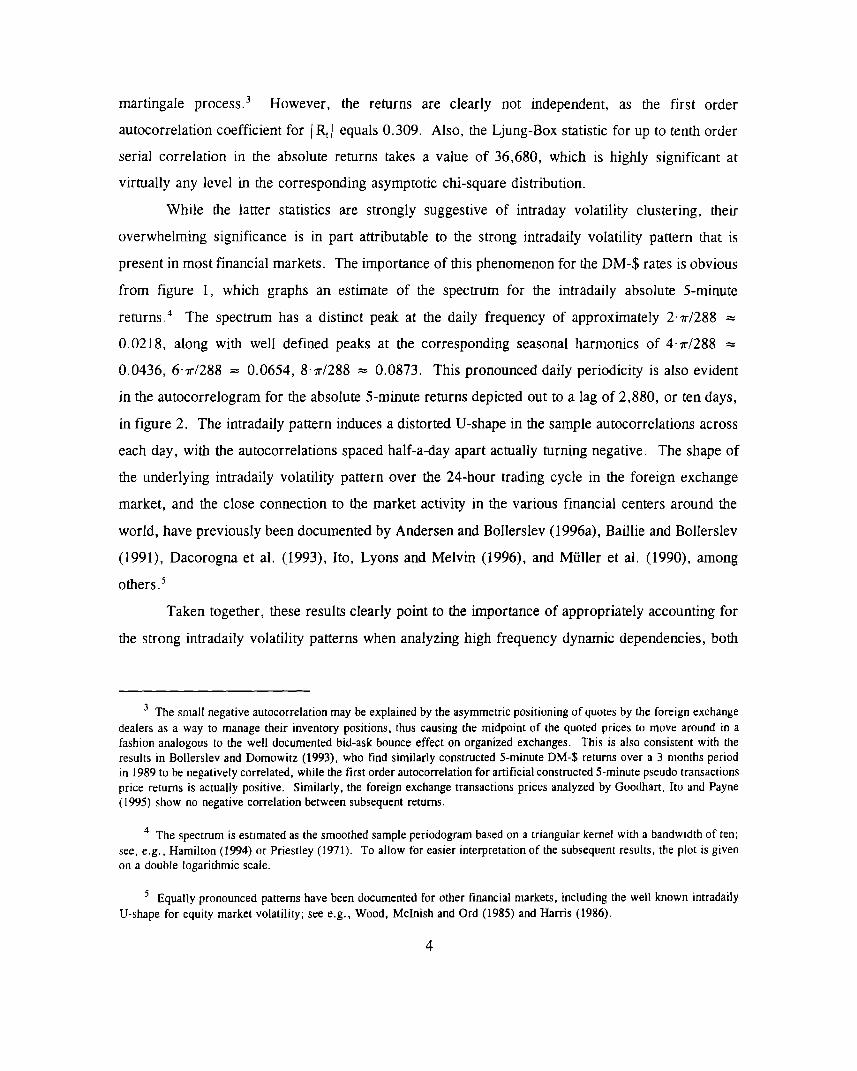
martingale process. 3 However, the returns are clearly not independent, as the first order

autocorrelation coefficient for IR!I equals 0.309. Also, the Ljung-Box statistic for up to tenth order

serial correlation in the absolute returns takes a value of 36,680, which is highly significant at

virtually any level in the corresponding asymptotic chi-square distribution.

While the latter statistics are strongly suggestive of intraday volatility clustering, their

overwhelming significance is in part attributable to the strong intradaily volatility pattern that is

present in most financial markets. The importance of this phenomenon for the DM-$ rates is obvious

from figure 1, which graphs an estimate of the spectrum for the intradaily absolute 5-minute

returns. 4 The spectrum has a distinct peak at the daily frequency of approximately 2 m/288 =

0.0218, along with well defined peaks at the corresponding seasonal harmonics of 4“m/288 =

0.0436, 6“T1288 = 0.0654, 8. Ir/288 = 0,0873. This pronounced daily periodicity is also evident

in the autocorrelogram for the absolute 5-minute returns depicted out to a lag of 2,880, or ten days,

in figure 2, The intradaily pattern induces a distorted U-shape in the sample autocorrelations across

each day, with the autocorrelations spaced half-a-day apart actually turning negative. The shape of

the underlying intradaily volatility pattern over the 24-hour trading cycle in the foreign exchange

market, and the close connection to the market activity in the various financial centers around the

world, have previously been documented by Andersen and Bollerslev (1996a), Baillie and Bollerslev

(1991), Dacorogna et al, (1993), Ito, Lyons and Melvin (1996), and Muller et al, (1990), among

others.5

Taken together, these results clearly point to the importance of appropriately accounting for

the strong intradaily volatility patterns when analyzing high frequency dynamic dependencies, both

3 The small negative autocorrelation may be explained by the asymmetric positioning of quotes by the foreign exchangedealers as a way to manage their invento~ positions, thus causing the midpoint of the quoted prices to move around in afashion analogous to the well documented bid-ask bounce effect on organized exchanges. This is also consistent with theresults in Bollerslev and Domowitz (1993), who Ftnd similarly constructed 5-minute DM-$ returns over a 3 months periodin 1989 to be negatively correlated, while the first order autocomelation for artificial constructed 5-minute pseudo transactionsprice returns is actually positive. Similarly, the foreign exchange transactions prices analyzed by Goodhart, Ito and Payne(1995) show no negative correlation between subsequent returns.

4 The spectrum is estimated as the smoothed sample periodogram based on a triangular kernel with a bandwidth of ten;see, e.g, , Hamilton (1994) or Priestley (1971). To allow for easier interpretation of the subsequent results, the plot is givenon a double logarithmic scale.

5 Equally pronounced patterns have been documented for other financial markets, including the well known irrtradailyU-shape for equity market volatility; see e.g., Wood, McInish and Ord (1985) and Harris (1986).

4

within and across different markets. However, even after explicitly modeling the typical intradaily

patterns, several recent studies have found that the estimation of standard GARCH type models for

the non-periodic intradaily volatility clustering tends to falter, in the sense rhat the estimated

parameters obtained for different intradaily sampling frequencies are at odds with the temporal

aggregation results developed by Drost and Nijman (1993), as well as the consistency theorems for

continuous time diffusions and misspecified ARCH models derived by Nelson (1990, 1992); for

existing evidence along these lines pertaining to the DM-$ rates analyzed here see Andersen and

BoIlerslev (1996a), Ghose and Kroner (1996) and Guillaume, Pictet and Dacorogna (1995). Thus,

it appears that multiple volatility components are necessarily required in order to fully explain the

complex intradaily dependencies that are present in all the major financial markets. b

factors

figures

release

The attempt to associate each of the underlying volatility components with explicit economic

seems destined to fail. Meanwhile, the regularly scheduled releases of macroeconomic

have been shown to induce heightened overall volatility immediately following the “news”

for a number of different financial instruments; for studies on the impact of macroeconomic

announcements on high-frequency foreign exchange rates see Andersen and Bollerslev (1996b),

Eddelbtittel and McCurdy (1996), Ederington and Lee (1993, 1995a, 1995b), Goodhart et al, (1993),

Harvey and Huang (1991), Hogan and Melvin (1994), Ito and Roley (1987), and Payne (1996). Not

surprisingly, the actual effect tends to vary according to the type of announcement. From the

analysis in Andersen and Bollerslev (1996b) the three regularly scheduled macroeconomic

announcements with the largest instantaneous impact on DM-$ volatility during the present sample

period are the U.S. Employment Report, the biweekly Bundesbank meetings and the U.S. Durable

Goods figures.’ To gauge the dynamic impact of each of these events, we consider the following

simple AR(1) model for the standardized five-minute DM-$ absolute returns, augmented by a

separate short-lived AR(1) component,

6 A multiple components, or Heterogeneous, ARCH model have been proposed by Muller et al. (1995) to explicitlycap[ure this phenomenon in the modelling of high-frequency foreign exchange returns. Components type model for dailystock return and interest rate volatility have also been estimated by Engle and Lee (1993) and Palm and Urbain (1995), andJones, Lament and Lurnsdaine (1996), respectively.

7 The U.S. Employment Report, Durable Goods figures, and Business Inventories analyzed below, are all amountedon a monthly schedule.

5

/RJ = y + yN”IN(t)+ @J/R,.,/ + 4~”D~(t)” IRC.ll + ~[, (1)

where the IJt) indicator variable equals unity if an amouncement of the given type, N, occurred

during the t‘th time interval and zero otherwise, while the “news” dummy, D~(t), equals unity for

the two hours immediately following the event; i.e., D~(t) = I~(t) + I~(t-l) + . . . + IJt-23). In

order to avoid confounding the dynamic dependencies by the strong intradaily volatility patterns, the

returns in equation (1) are standardized by the average absolute return for the particular 5-minute

interval; i.e. , 1~1 = 260” IR(,.[).zgg+”[ (~;:!l%r-l)zsg+nl)-’ for n=l>2!..!288! and ~=1,2,.,260.8

The first order sample autocorrelation for these standardized returns, i.e., IJt) and D~(t) = O for

all t, equals ~ = 0.273. However, the estimates obtained from the simple descriptive model in

equation (1) suggest that the three major amouncements result in their own distinct volatility

response pattern. Specifically, for the Employment Report $~ = 5.346 (1.424) and d~ = -O.081

(0.050), respectively, where the numbers in parentheses represent robust standard errors. These

estimates therefore indicate an immediate increase in the volatility, but largely unaltered short-run

dynamic dependencies in the two hours following the release of the report. Meanwhile, the estimates

for the Bundesbank biweekly meetings are 1.394 (O.651) and 0.102 (0.054), suggestive of a slower

rate of decay in the volatility component associated with this “news” release. The Durable Goods

report also elevates volatility, $N = 1.801 (0.687), but the estimated short-run decay is actually

faster than average with & = -0.130 (O.037), or j + & = 0.144, Many other announcements

share this dynamic pattern. For instance, for the Business Inventory figures the same two parameters

are O.021 (O.11O) and -0.094 (O.045), respectively.

This relatively rapid decay of the readily identifiable “news” effects at the intradaily

frequencies is in sharp contrast to the well documented highly persistent volatility clustering that is

present at the lower interdaily frequencies. A voluminous literature surveyed in Bollerslev, Chou

and Kroner (1992) have argued that the volatility processes for most speculative returns are close to

being integrated in the variance in the sense of the IGARCH model of Engle and Bollerslev (1986);

for evidence pertaining to daily foreign exchange rates see, e, g., Baillie

Bollerslev and Engle (1993) and Hsieh (1989). More recently however,

and Bollerslev (1989),

Baillie, Bollerslev and

8 Much more elaborate standardization procedures for characterizing the average intradaily volatility patterns haverecently been developed by Andersen and Bollerslev (1996a, 1996b) and Dacorogna et al, (1993).

6

Mikkelsen (1996), Dacorogna et al. (1993), and Harvey (1994), have questioned these earlier

findings, on the grounds that the long-run dependence in the volatility of interdaily foreign exchange

returns is better characterized by a slowly mean-reverting fractionally integrated process, 9 While

shocks to the daily volatility process are highly persistent, it appears that they eventually dissipate,

albeit at a very slow hyperbolic rate. As discussed in section 4, the approximate linear behavior of

the estimated spectrum for IR, 1, when plotted on the double logarithmic scale in figure 1, is

consistent with this long-memory type dependence. Similarly, the rapid initial decay followed by

the decidedly slower rate of dissipation for the longer-run autocorrelations in figure 2 are also

suggestive about the existence of long-memory type dependencies, although the marked intradaily

periodicity severely complicates the interpretation of the overall pattern in the autocorrelogram for

the raw absolute returns.

3. THE THEORETICAL VOLATILITY MODEL

This section demonstrates that the mixture-of-distributions hypothesis, originally advocated by Clark

(1973), Epps and Epps (1976), and Tauchen and Pitts (1983), provides a framework for rationalizing

the complicated, and seemingly conflicting, behavior of the return volatility dynamics that exist at

the inter- and intradaily frequencies; see also the analyses in Andersen (1996), Harris (1987), Ross

(1989), and Taylor (1994). Intuitively, the mixture-of-distributions hypothesis stipulates that the

return generating process reflects the impact of a large number of imovations to the information

processes associated witi the economic factors of relevance for the valuation of the asset in question.

While the imovations, by definition, are serially uncorrelated, they are not likely to be independent

since information of a particular kind tends to be positively autocorrelated, thus inducing the kind

of dependence in the absolute, or second order, moments of the returns discussed above.

To formalize these ideas, consider the following representation for the intradaily returns,

(2)

9 Similar long-run dependencies in daily stock market volatility have been observed by Bollerslev and Mikkelsen ( 1996a,1996b), Breidt, Crato and de Lima (1995), Ding and Granger (1996), Ding, Granger and Engle (1993), Gallant, Hsieh andTauchen (1994), Granger and Ding (1996a, 1996b), Liu (1995), and McCurdy and Michaud (1996).

7

where m~denotes the conditional mean of the raw returns, rl , Z, is an i. id. stochastic process with

mean zero and variance one, and the non-negative, positively serially-correlated mixing variable, V, ,

serves as a proxy for the aggregate amount of information flow to the market. Equation (2) assumes

the typical form associated with the discrete time ARCH class of models in which both m, and V,

are assumed measurable with respect to the time t-1 observable information set, so that the

conditional variance of the return equals Vart.[(~ ) = Var~.i(r, ) = V, . More generally, however,

the information flow is not directly observable, and V, is naturally modeled as a latent, or stochastic,

volatility process; see, e.g., Andersen (1992) for further discussion. Of course, lacking additional

assumptions regarding the temporal dependencies in the V, process, the model in equation (2) is void

of testable empirical implications in regards to the observed volatility dynamics.

The rest of this section develops a specific representation of equation (2) that affords an

interpretation of volatility as governed by heterogeneous information arrivals, while retaining the

capacity of reconciling the seemingly conflicting evidence regarding volatility at the various return

frequencies, and producing interesting empirical implications that are directly testable.

3.1 Volatility as a Manifestation of Heterogeneous Information Arrivals

Motivated by the empirical observations in section 2, we assume that the volatility process reflects

the aggregate impact of N distinct information arrival processes; say Vj,~>0, where j = 1, 2, . . . ,N.

Also, following Andersen (1994), the temporal dependence of each constituent component is

expressed in terms of a standard log-normal stochastic volatility, or Exponential SARV, model,

Vj, [ = O!j” Vj, [.[ + tj, [ , (3)

where ~j,t ~ ln(Vj,, ) - ~j , ~j = E[ln(Vj,r )], and the ~j,~’sare assumed to be i.i.d. N(O,~ ) for all j,

j=l,2 ,, ... N. The logarithmic formulation in equation (3) ensures that the number of information

arrivals dictated by the j ‘th component process, Vj,l = exp(~j,, + ~j ), is positive. The autoregressive

coefficient, ~j , reflects the degree of persistence in the j ‘th information arrival process. Consistent

with the notion of positively serially-correlated but stationary “news” arrivals, we restrict these

parameters to fall within the unit interval; i.e., O < Uj < 1.

According to the mixture-of-distributions hypothesis, each information arrival process has an

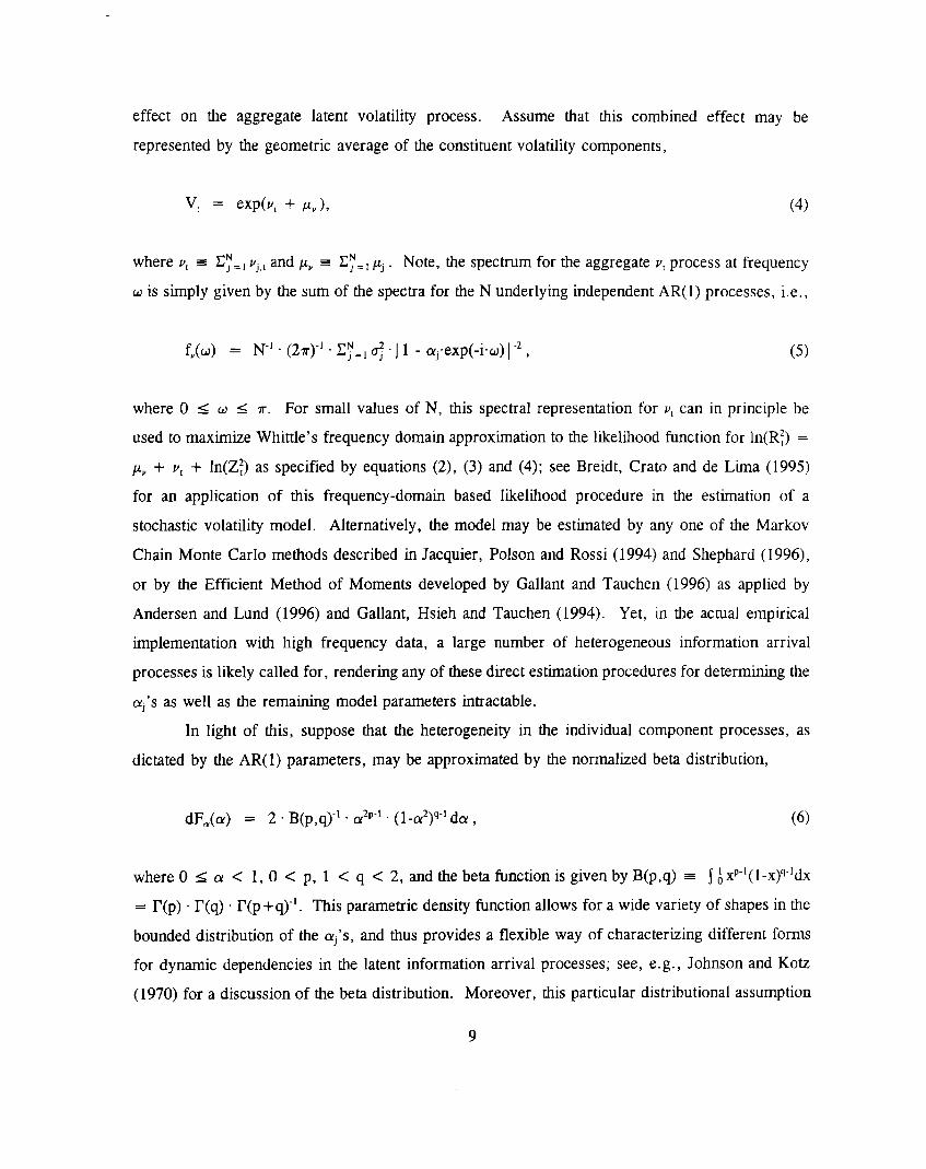
effect on the aggregate latent volatility process. Assume that this combined effect may be

represented by the geometric average of the constituent volatility components,

V, = exp(v, + p.), (4)

where V[ = Z!., JJj,tand p, = Z!. ~pj . Note, the spectrum for the aggregate v, process at frequency

u is simply given by the sum of the spectra for the N underlying independent AR(1) processes, i.e.,

where O < ti < m. For small values of N, this spectral representation for v, can in principle be

used to maximize Whittle’s frequency domain approximation to the likelihood function for ln(R~) =

p, + v, + ln(Z~) as specified by equations (2), (3) and (4); see Breidt, Crato and de Lima (1995)

for an application of this frequency-domain based likelihood procedure in the estimation of a

stochastic volatility model. Alternatively, the model may be estimated by any one of the Markov

Chain Monte Carlo methods described in Jacquier, Poison and Rossi (1994) and Shephard (1996),

or by the Efficient Method of Moments developed by Gallant and Tauchen (1996) as applied by

Andersen and Lund (1996) and Gallant, Hsieh and Tauchen (1994). Yet, in the actual empirical

implementation with high frequency data, a large number of heterogeneous information arrival

processes is likely called for, rendering any of these direct estimation procedures for determining the

~j’s as well as the remaining model parameters intractable.

In light of this, suppose that the heterogeneity in the individual component processes, as

dictated by the AR(1) parameters, may be approximated by the normalized beta distribution,

dFa(a) = 2 “B(p,q)-l “cr’p-i“(1-a2)q”1da , (6)

where O < a < 1, 0 < p, 1 < q < 2, and the beta function is given by B(p,q) = ~~xP-l(l-x)q-ldx

= I_’(p)“l?(q) “17(p+q)-l. This parametric density function allows for a wide variety of shapes in the

bounded distribution of the ~j ‘s, and thus provides a flexible way of characterizing different forms

for dynamic dependencies in the latent information arrival processes; see, e.g., Johnson and Kotz

(1970) for a discussion of the beta distribution. Moreover, this particular distributional assumption

9

regarding the heterogeneity in the underlying Pj,[ processes has a number of testable implications in

regards to the dynamic dependencies in the observable process for the absolute returns.

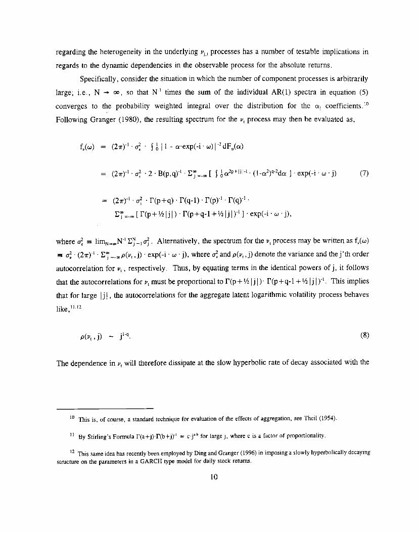
Specifically, consider the situation in which the number of component processes is arbitrarily

large; i.e., N ~ m, so that N-l times

converges to the probability weighted

Following Granger (1980), the resulting

the sum of the individual AR(1) spectra in equation (5)

integral over the distribution for the ~j coefficients. 10

spectrum for the Vtprocess may then be evaluated as,

fV(u) = (27r)-1~~ c j ~ I1- a“exp(-i” U) I‘2dFm(a)

= (27r)-1“~ ~2 I B(p,q)-l “E~=.a [ \ &IY2P+lJ1-[~(1-ci2)q-2da] exp(-i u “j) (7)

= (2m)-1”~ “r(p+q) I r(q-1)” r(pyl” r(q)-”

E;=.m[Np+kljl) “I’(p+q-l+ ’/21jl)-’] “exp(-i’u” j),

where ~ = lim~.. N-l Ey.l ~. Alternatively, the spectrum for the v, process maybe written as f,(u)

= ~ “(27r)-’“Em, =.~ P(v,, j) “exp(-i” u “j), where < and P(P,, j) denote the variance and the j’th order

autocorrelation for V[, respectively. Thus, by equating terms in the identical powers of j, it follows

that the autocorrelations for v, must be proportional to r(p + % Ij I)” J7(p+ q-1 + % Ij I)-1. This implies

that for large Ij 1, the autocorrelations for the aggregate latent logarithmic volatility process behaves

llke,lllz

P(vL, j) - jl-q. (8)

The dependence in v, will therefore dissipate at the slow hyperbolic rate of decay associated with the

10 This is of course, a standard technique for evaluation of [he effects of aggregation, see Theil (1954).

“a-bfor large j, where c is a factor of proportionality.11 By Stirling’s Formula I’(a+j).I’(b+j)”[ = C.J

12 This same idea has recently been employed by Ding and Granger (1996) in imposing a slowly hyperbolically decayingstructure on the parameters in a GARCH type model for daily stock returns.

10

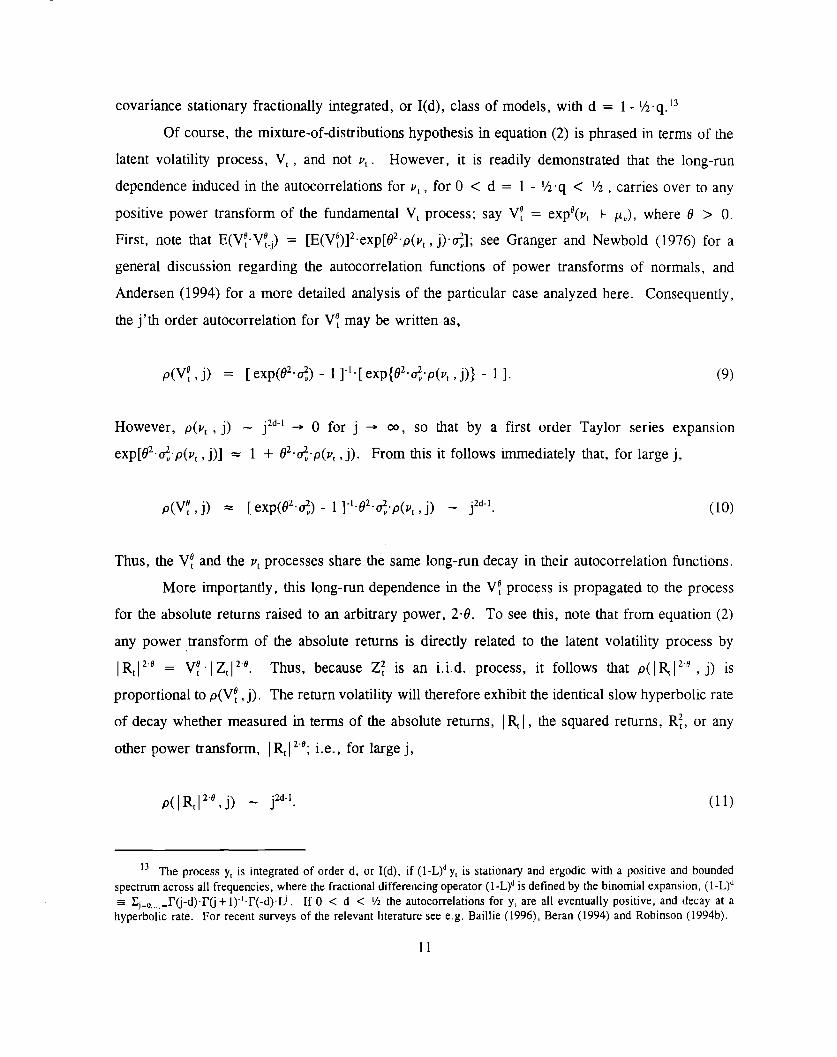
covariance stationary fractionally integrated, or I(d), class of models, with d = 1- YZ.q,’3

Of course, the mixture-of-distributions hypothesis in equation (2) is phrased in terms of the

latent volatility process, V, , and not Vt. However, it is readily demonstrated that the long-run

dependence induced in the autocorrelations for v, , for O < d = 1- %q < % , carries over to any

positive power transform of the fundamental V, process; say V: = expd(v, + p,), where 0 > 0.

First, note that E(V~”V[_j)= [E(V~)]2exp[02”p(v, , j) ~]; see Granger and Newbold (1976) for a

general discussion regarding the autocorrelation functions of

Andersen (1994) for a more detailed analysis of the particular

the j’ th order autocorrelation for V? may be written as,

power transforms of normals, and

case analyzed here. Consequently,

P(Y, j) = [exp(02”~) -1 ]-’”[exp{02~p(~,, j)} - 1]. (9)

However, p(v, , j) - j2d-’ + O for j ~ m, so that by a first order Taylor series expansion

exp[oz”~”~(~t, j)] = 1 + 02”~’p(v,, j). From this it follows immediately that, for large j,

P(V!, j) = [exp(~’~) -1 ]-’02”~op(u,, j) - j2d-’, (lo)

Thus, the V; and the v, processes share the same long-run decay in their autocorrelation functions,

More importantly, this long-run dependence in the V: process is propagated to the process

for the absolute returns raised to an arbitrary power, 2-6. To see this, note that from equation (2)

any power transform of the absolute returns is directly related to the latent volatility process by

lRt12° = V: IZ,12”. Thus, because Z: is an i, id. process, it follows that P( I~ 12“’, j) is

proportional to P(V:, j). The return volatility will therefore exhibit the identical slow hyperbolic rate

of decay whether measured in terms of the absolute returns, I~ 1, the squared returns, R?, or any

other power transform, IR, 12“0;i.e., for large j,

P(lR[120 , j) - jz”-1.(11)

13 The process y, is integrated of order d, or I(d), if (1-L)~y, is stationa~ and ergodic with a positive and boundedspectrum across all frequencies, where the fractional differencing operator (1-L)~ is deftned by the binomial expansion, ( l-L)~= z.,_O,,,mI’&d).l_’Q+ 1)”1.I’(-d) LJ. If O < d < M the autocomelations for y, are all eventually positive, and decay at ahyperbolic rate. For recent surveys of the relevant literature see e.g. Bail lie (1996), Beran (1994) and Robinson (1994b).

11

This result is important because it demonstrates how the long-memory features of volatility may arise

naturally through the interaction of a large number of diverse information processes. From a

conceptual perspective, it implies that the long-memory characteristics reflect inherent properties of

the return generating process, rather than external shocks that induce a structural shift in the volatility

process, as, e.g., suggested by Lamoureux and Lastrapes (1990). In other words, the mechanism

responsible for the fractional integration in volatility is generic to the returns process, and thus ever

present, so that with high frequency data it may be feasible to identify the manifestation of the

phenomenon even over relatively short spans of calendar time. We pursue this possibility in section

4.

For now, we simply note that the result in equation (11) is consistent with the empirical

behavior of the autocorrelograms for the various power transforms of daily equity returns reported

in Ding, Granger and Engle (1993). Although Harvey and Streibel (1996) argue that it is

impossible, by theoretical means, to ascertain which value of 0 will uniformly maximize the

autocorrelations for the simple stochastic volatility model, corresponding to N = 1 in the current

setup, it is noteworthy that the sample autocorrelations for the daily returns analyzed in Ding,

Granger and Engle (1993) attain their maxima for 0 very close to one-half. 14 Motivated by this

observation, we concentrate on the correlation structure for the intradaily absolute returns in the

empirical investigations reported on below. 15

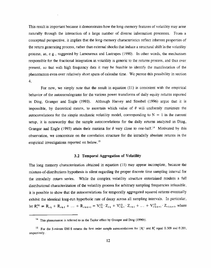
3.2 Temporal Aggregation of Volatility

The long memory characterization obtained in equation (11) may appear incomplete, because the

mixture-of-distributions hypothesis is silent regarding the proper discrete time sampling interval for

the intradaily return series. While the complex volatility structure entertained renders a full

distributional characterization of the volatility process for arbitrary sampling frequencies infeasible,

it is possible to show that the autocorrelations for temporally aggregated squared returns eventually

exhibit the identical long-run hyperbolic rate of decay across all sampling intervals. In particular,

let Rfk) = RT.~+ R,.~.l + . . . + RT~.~+l= v:? “Z,.k + v;~-1 “Z,.k.l + . . . + ‘Yt.k+l “‘,k-k+l, where

14 This phenomenon is referred to as the Taylor effect by Granger and Ding (1996b).

15 For the 5-minute DM-$ returns the first order sample autocomelations for I~ I and R; equal 0.309 and 0.201,

respectively.

12

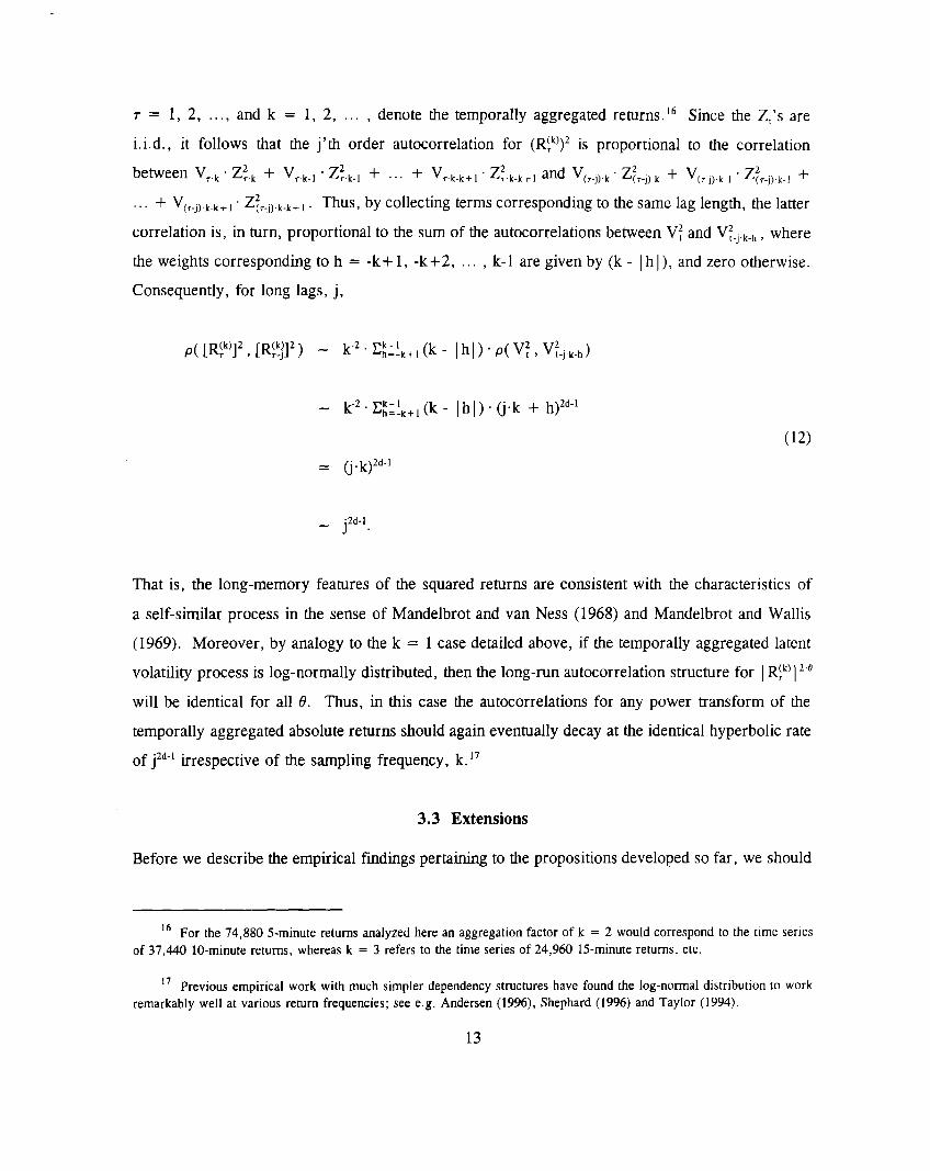
~ = 1,2, . . . . andk = 1,2, . . . , denote the temporally aggregated returns. ‘b Since the Z[’s are

i. i.d., it follows that the j ‘th order autocorrelation for (R~k))2is proportional to the correlation

between Vr.~“Z~.~+ V,.~.l - Z~.~_l+ . . . + vr.k.~+l~Z*.7 k-k+ I and ‘(r-j)k “ ‘?r-j)k + ‘(r-j) k-l “ z~,.,),k., +

. . + ‘(~-j)k-k+1 ‘ ‘~r.j)k-k+I Thus, by collecting terms corresponding to the same lag length, the latter

correlation is, in turn, proportional to the sum of the autocorrelations between V? and V~.j.k.~, where

the weights corresponding to h = -k+ 1, -k+2, . . . . k-1 are given by (k - Ih I), and zero otherwise.

Consequently, for long lags, j,

k-2“E~j!k+l (k - Ihl) . (jk + h)2d-1

(12)

= (j .k)z’-l

- j2d-1.

That is, the long-memory features of the squared returns are consistent with the characteristics of

a self-similar process in the sense of Mandelbrot and van Ness (1968) and Mandelbrot and Wallis

(1969). Moreover, by analogy to the k = 1 case detailed above, if the temporally aggregated latent

volatility process is log-normally distributed, then the Iong-mn autocorrelation structure for I~) Iz0

will be identical for all 6. Thus, in this case the autocorrelations for any power transform of the

temporally aggregated absolute returns should again eventually decay at the identical hyperbolic rate

of jzd-(“urespective of the sampling frequency, k. 17

3.3 Extensions

Before we describe the empirical findings pertaining to the propositions developed so far, we should

16 For the 74,880 5-minute returns analyzed here an aggregation factor of k = 2 would correspond to the Limeseriesof 37,440 10-minute returns, whereas k = 3 refers to the time series of 24,960 15-minute returns, etc.

17 Previous empirical work with much simpler dependency structures have found the log-normal distribution to workremarkably well at various return frequencies; see e.g. Andersen (1996), Shephard (1996) and Taylor (1994).

13

emphasize that the theoretical model readily accommodates extensions in a number of directions

which allow for added flexibility and realism in the portrayal of the volatili~ dynamics without

affecting the salient long-nm dependencies. Firstly, the mixture-of-distributions hypothesis in

equations (2), (3) and (4) obviously neglects the repetitive intradaily pattern in the volatility that is

evident in the spectrum and the autocorrelogram for the 5-minute absolute DM-$ returns in figures

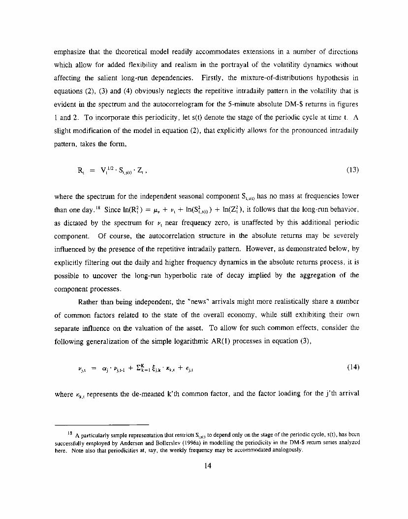
1 and 2. To incorporate this periodicity, let s(t) denote the stage of the periodic cycle at time t. A

slight modification of the model in equation (2), that explicitly allows for the pronounced intradaily

pattern, takes the form,

(13)

where the spectrum for the independent seasonal component S1,,([)has no mass at frequencies lower

than one day. 18 Since ln(R~ ) = p + v~+ ln(S~~(~)) + ln(Z~ ), it follows that the long-run behavior,v

as dictated by the spectrum for v~near frequency zero, is unaffected by this additional periodic

component. Of course, the autocorrelation structure in the absolute returns may be severely

influenced by the presence of the repetitive intradaily pattern. However, as demonstrated below, by

explicitly filtering out the daily and higher frequency dynamics in the absolute returns process, it is

possible to uncover the long-run hyperbolic rate of decay implied by the aggregation of the

component processes.

Rather than being independent, the “news” arrivals might more realistically share a number

of common factors related to the state of the overall economy, while still exhibiting their own

separate influence on the valuation of the asset. To allow for such common effects, consider the

following generalization of the simple logarithmic AR(1) processes in equation (3),

where ~~~represents the de-meaned k’ th common factor, and the factor loading for the j‘ th arrival

18 A particularly simple representation that restricts S,.,(,)to depend ody on the stage of the periodic cycle. s(t), has beensuccesstldly employed by Andersen and Bollerslev (1996a) in modelling the periodicity in the DM-$ return series analyzedhere. Note also that periodicities at, say, the weekty frequency may be accommodated analogously.

14

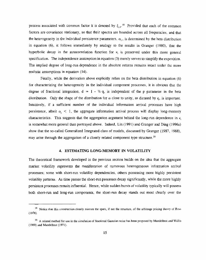
process associated with common factor k is denoted by ~j,~.19 provided that each of the common

factors are covariance stationary, so that their spectra are bounded across all frequencies, and that

the heterogeneity in the individual persistence parameters, aj , is determined by the beta distribution

in equation (6), it follows immediately by analogy to the results in Granger (1980), that the

hyperbolic decay in the autocorrelation function for V, is preserved under this more general

specification. The independence assumption in equation (3) merely serves to simplify the exposition.

The implied degree of long-run dependence in the absolute returns remains intact under the more

realistic assumptions in equation (14).

Finally, while the derivation above explicitly relies on the beta distribution in equation (6)

for characterizing the heterogeneity in the individual component processes, it is obvious that the

degree of fractional integration, d = 1 - lA”q, is independent of the p parameter in the beta

distribution. Only the shape of the distribution for a close to unity, as dictated by q, is important.

Intuitively, if a sufficient number of the individual information arrival processes have high

persistence, albeit ~j < 1, the aggregate information arrival process will display long-memory

characteristics, This suggests that the aggregation argument behind the long-n.m dependence in Vt

is somewhat more general than portrayed above. Indeed, Lin ( 1991) and Granger and Ding (1996a)

show that the so-called Generalized Integrated class of models, discussed by Granger

may arise through the aggregation of a closely related component type structure. 20

4. ESTIMATING LONG-MEMORY IN VOLATILITY

The theoretical framework developed in the previous section builds on the idea that

(1987, 1988),

the aggregate

market volatili~ represents the manifestation of numerous heterogeneous information arrival

processes; some with short-run volatility dependencies, others possessing more highly persistent

volatility patterns. As time passes the short-run processes decay significantly, while the more highly

persistent processes remain influential. Hence, while sudden bursts of volatility typically will possess

both short-run and long-inn components, the short-run decay stands out most clearly over the

19 NO~lCe~hat~hi~~On~tmctloncloselymirrorsthe spirit, if not the struCtUR, of the arbitrage Pricing theow of ‘Oss

(1976).

20 A related method for use in the simulation of fractional Gaussian noise has been proposed by Mandelbrot and Wallis(1969) and Mandelbrot (1971).

15

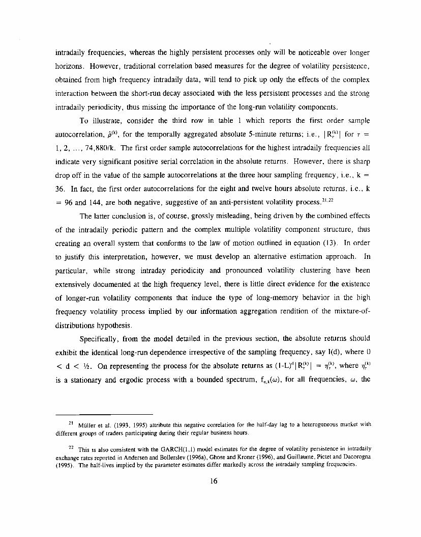
intradaily frequencies, whereas the highly persistent processes only will be noticeable over longer

horizons, However, traditional correlation based measures for the degree of volatility persistence,

obtained from high frequency intradaily data, will tend to pick up only the effects of the complex

interaction between the short-run decay associated with the less persistent processes and the strong

intradaily periodicity, thus missing the importance of the long-run volatility components.

To illustrate, consider the third row in table 1 which reports the first order sample

autocorrelation, j(k), for the temporally aggregated absolute 5-minute returns; i.e., IR~k)I for ~ =

1, 2, ,.., 74,880/k. The first order sample autocorrelations for the highest intradaily frequencies all

indicate very significant positive serial correlation in the absolute returns. However, there is sharp

drop off in the value of the sample autocorrelations at the three hour sampling frequency, i.e., k =

36. In fact, the first order autocorrelations for the eight and twelve hours absolute returns, i.e., k

= 96 and 144, are both negative, suggestive of an anti-persistent volatility process .2122

The latter conclusion is, of course, grossly misleading, being driven by the combined effects

of the intradaily periodic pattern and the complex multiple volatility component structure, thus

creating an overall system that conforms to the law of motion outlined in equation (13). In order

to justify this interpretation, however, we must develop an alternative estimation approach. In

particular, while strong intraday periodici~ and pronounced volatili~ clustering have been

extensively documented at the high frequency level, there is little direct evidence for the existence

of longer-inn volatility components that induce the type of long-memory behavior in the high

frequency volatility process implied by our information aggregation rendition of the mixture-of-

distributions hypothesis.

Specifically, from the model detailed in the previous section, the absolute returns should

exhibit the identical long-run dependence irrespective of the sampling frequency, say I(d), where O

< d < %. On representing the process for the absolute returns as (1-L)d I~k) I = ~~), where #)

is a stationary and ergodic process with a bounded spectrum, f~,k(~), for all frequencies, u, the

21 Muller et al. (1993, 1995) attribute this negative correlation for the half-day lag to a heterogeneous market wlthdifferent groups of traders participating during their regular business hours.

22 This is also consistent with the GARCH(l, 1) model estimates for the degree of volatility persistence in intradaily

exchange rates reported in Andersen and Bollerslev (1996a), Ghose and Kroner (1996), and Guillaume, Pictet and Dacorogna(1995). The half-lives implied by the parameter estimates differ markedly across the intradaily sampling frequencies.

16

spectrum for IR~k)I may therefore be written as,23

‘1RI ,k(”) = I [1 - exp(-i.~)]”d I2 “fq,k(u)

(15)

= I2sin(%u) I‘2””.f,,,(u) .

Since, lim&mU-l”sin(l/2.u) = ‘/2, it follows that for the frequencies close to zero, i.e., u = O,

f,RI,~(ti) = f~,@) 1~1-2’d, (16)

or,

ln[fl RI ,k(”)] = ln[f,,~(0)] -2 “d I in(u) . (17)

Hence, the spectrum should be approximately log-linear for the long-n-m frequencies. Indeed, when

viewed on the double logarithmic scale in figure 1, the spectrum for the 5-minute absolute returns,

i.e., k = 1, is very close to a straight line over the interdaily frequencies, O < u < 2“r/288 =

0.0218.

The Geweke and Porter-Hudak (1983) log-periodogram regression estimate for the fractional

order of integration is based directly on this relationship. These estimates for the dependence in

IR!’)1, obtained across all of the intradaily frequencies, are reported in the column labelled d~~) in

table 1. Formally,

where ti’,~,~ = (m-f)-l “~~=f+~~j,k, and IIRi,~(~j,k) denotes the sample periodogram for IR!’)I at the

j’ th Fourier frequency, i.e., ‘&)j,k = 2” m“j” k/T. Although this estimator for d has been fairly widely

used in the literature, consistency for O < d < % has only recently been established by Robinson

(1995) under regularity conditions that include the truncation and trimming parameters both tending

to infinity, albeit at a slower rate than the sample size; i.e., m - ~, 1 ~ m, I/m ~ O, and m“k/T

23 Formal conditions for the equivalence between this spectral definition of long-memory and the hyperbolic decay ratein the au[ocorrelation function are discussed in Beran (1994) and Robinson (1994b); see also Granger and Ding (1996a).

17

~ O. However, the regulari~ conditions also require that I~k) I be normally distributed, which in

turn implies that the estimator itself, d~~), is asymptotically normal with a variance equal to m-

1”(#/24), independent of the sample size, T/k.

For derivation of the results reported on in table 1, we took m = [(T/k)L’2]and 1?= [m’”],

respectively, where [“] denotes the integer value. However, in order to avoid any confounding

effects from frequencies corresponding to less than one day, the estimate for ~~~) is based on m =

255 and 1 = 3. Note that, in contrast to the sample autocorrelations reported in the ~(k)column, the

6~&)estimates for the degree of long-run volatility dependence are remarkably stable across the

different intradaily return intervals. In fact, when judged by the asymptotic normal distributions,

all of the estimates are within less than one asymptotic standard error of d = 0.359.24 To illustrate,

consider the estimate for &~) = O.321, corresponding to the average slope of the spectrum for the

5-minute absolute returns in figure 1 over the frequencies O < u s 255”2 T/74,888 = 0,0214.25

The theoretical standard error for this estimate equals m“(24255)-1’2 = 0.040. As such, the estimates

for k = 1, 2, . . . . 144 confirm the proposition that the degree of fractional integration in the absolute

returns is invariant with respect to the sampling frequency. 26

Unfortunately, the assumption of normality underlying the formal statistical justification for

the &.&)estimates is clearly violated in the present context. For instance, the sample skewness and

kurtosis for the absolute 5-minute returns equal 0.367 and 21.5, respectively. The last column in

table 1 therefore reports the results from a less restrictive semiparametric estimation procedure for

determining d, based on the ratio of the periodogram for two frequencies close to zero. 27 To

motivate this estimator, let

(19)

24 This value of d corresponds to the estimated hyperbolic decay rate in the low-pass filtered 5-minute absolute returns

described further in section 5 below.

25 Including all of the frequencies up to j = [74,880”2] = 273, the estimate for d&) drops to a value of only 0.242,highlighting the importance of explicitly excluding the intradaily effects in the estimation.

26 This is also consistent with the notion of an intrinsic time scale in the foreign exchange market as discussed by Mi-illeret al. (1993).

27 The same log-Perlodogram and average periodogram estimators for d implemented here have Previously been

employed by Delgado and Robinson (1994) in the analysis of a time series of monthly Spanish inflation rates.

18

denote the average periodogram for the frequencies j = 1, 2, . . . . m. Then, following Robinson

(1994a), for O < d < 1Aand m+ m, but ink/T -0,

ln(G~,, ) - ln(G1,~l,~) + (1 -2 “d)” h(q) = 0, (20)

where O < q < 1. Thus, upon rearranging the terms in equation (20), the following estimator for

d becomes apparent,

(21)dfi) = % + % “in(q)-’ [ln(G~,k) - ln(G[,~l,, )1.

Consistency of this frequency-domain estimator for d has been established by Robinson (1994a)

under much weaker regularity conditions than those available for d~~), Furthermore, given the

assumption of normality underlying the existing consistency proof for the log-periodogram estimator,

~~~), Lobato and Robinson (1996) have recently shown that the alternative ~~~) estimator is

asymptotically normal for O < d < %, but non-normally distributed for M < d < %.

The estimates reported in the last column of table 1 are based on a truncation parameter of

m = [(T/k)l’2] for k = 2, 3, ,.., 144, whereas m = 255 for k = 1 in order to avoid any

confounding effects from the intradaily dependencies in the estimation of d~~). The value for the

scalar q was fixed at 0,25 across all the sampling frequencies. In line with the simulation evidence

reported in Lobato and Robinson (1996), some informal sensitivity analysis revealed the results to

be fairly robust with respect to this choice. Turning to the actual estimates, the similarities across

the different values of k are even more striking than for the log-periodogram estimates. The average

value of ~~~)equals 0.321, while ranging from a low of 0.270 for k = 72 to a high of only 0.385

for k = 1.28

Consistent with the notion of a heterogeneous component structure and the invariance under

temporal aggregation, these estimates for d, based on a single year of intradaily returns, are also

very much in line with previously reported estimates for much longer time spans of daily data, For

instance, on calculating the same Iog-periodograrn regression and average periodogram estimates for

the fractional order of integration for the time series of 3,649 daily DM-$ absolute returns from

28 The estimate for ~~~)corrupted by the intradaily frequencies, or j = 256, 257, . . . . 273, equals 0.172.

19

March 14, 1979 through September 29, 1993, the estimates are 0.344 and 0.301, respectively. z9

Thus, the relatively simple semiparametric frequency-domain estimators in equations (18) and (2 1)

are both capable of uncovering the inherent long-run volatility dependencies in the time series of

high-frequency intradaily returns, without having to impose any specific structure on the short-run

behavior of the system in order to accommodate the complex intradaily dynamics and repetitive

periodic patterns that corrupt the conventional correlation based measures.

To further appreciate the notion of long-memory volatility dynamics, consider the properties

of the (1-L)d filter designed to annihilate the long-run dependence in the absolute returns. Expressing

the fractional differencing operator in terms of its binomial expansion, the gain of the corresponding

filter may be written as,

I[1 - exp(-iu)]d I = { [Z.-,-0, ,,maj“CMO”J)12+ [ ‘j=(l,,,mbj sin(uj) ]2 }“2, (22)

where O < u < r, and bj = llj-d) “I’(j+l)-l “r(-d) for j = O, 1, . . Intuitively, the gain at

frequency u represents the magnitude by which the filter multiplies the component of the time series

with a repetitive cycle of 2”T/U periods. The enhanced flexibility provided by allowing for fractional

orders of integration is evident from figure 3, which plots the gains of (1-L~ for d = O, 0.25, 0.359,

0.5, and 1. Although all the fractional differencing operators with d > 0 completely eliminate the

zero frequency component, the filters differ greatly in terms of their gains over the finite frequencies,

0 < u < m.’” The filter gain of [2 -2 ICOS(U)]l’2for the first difference operator, (1-L), associated

with the Integrated GARCH, or IGARCH, class of models for ~, implies a much greater down-

weighting of the long-run dependencies than the fractional differencing filter with d = 0.359.

The justification, within the frequency domain, of filtering the five-minute DM-$ absolute

returns by (1-L)O-359is evident from the plot of the estimated spectrum for (1-L)0359I~ ) given in

29 Both estimates are based on m = 168 corresponding to a period of 3 ,648/ 168 = 21.7 trading days, or approximately

one month, along with ( = 4 and q = 0.25.

313Since the autocorrelatlons of a long-memory process with d > 0 is not summable, all of the (1-L)~ filters necessarily

eliminate the zero frequency component in order to achieve a bounded spectrum for the fractionally difference series.

20

figure 4.3’ The flat spectrum for O < u < 2cT/288 = 0,0218 reveals that the fractional

differencing operator is, indeed, successful in eliminating the longer-run dependencies. At the same

time, the pronounced peaks associated with the daily periodicity remain very similar across figures

1 and 4. These results are further underscored by the time-domain autocorrelogram for (1-L)0359I~ I

depicted in figure 5. Although more noisy, the autocorrelations exhibit the same repetitive daily

cycles as the autocorrelations for the raw absolute returns in figure 2.3* However, in contrast to

the autocorrelogram for the raw absolute returns, which display an overall slow hyperbolic rate of

decay, the daily periodic patterns in the autocorrelogram for the fractionally difference five-minute

absolute returns are centered on zero. ‘- -,. . . .,.

l’he Iong-mn dependence m the series has been ehrmnated.

5. LOW-PASS FILTERING AND LONG-RUN VOLATILITY DYNAMICS

outlined in the previous section allow for the determinationThe frequency domain based estimators

of the degree of long-run volatili~ dependence across the different sampling frequencies by explicitly

focussing on tie shape of the spectrum around the origin. Alternatively, a non-structural time-

domain estimation procedure could be based on the eventual hyperbolic decay of the autocorrelation

function implied by the presence of long-memory. However, as the sample autocorrelogram for the

five-minute absolute returns in figure 2 clearly illustrates, the implementation of this idea is obscured

by the strong intradaily periodicity. Various standardization procedures have previously been

proposed for modeling the systematic intradaily patterns in the volatility of high frequency foreign

exchange rates, including the time-deformation approach advocated by Muller et al. (1990) and

Ghysels and Jasiak (1995), and the flexible Fourier functional form utilized by Andersen and

Bollerslev (1996a, 1996b) .33 These procedures are directly applicable in a forecasting context. In

contrast, the low-pass filtering technique developed below is

of both past and future absolute returns. By explicitly

based on a two-sided weighted average

annihilating the dependencies with a

31 The binomial expansion for (l-L) 0’59was truncated at a lag length of 1440, corresponding to one week. Also,

following Baillie, Bollerslev and Mikkelsen (1996) all of the pre-sample values for I~ I were fixed at their unconditionalsample analogues.

32 Note that the scales for the two autocomelograms differ across figures 2 and 5, Also, the first order sampleautocorrelation of -0.160 for (1-L)O’59I~ I does not fit on the scale in figure 5.

33 The notion of time deformation also underlies the motivation behind the Autoregressive Conditional Duration modelin Engle and Russell (1996).

periodicity of less than one day, the in-sample low-pass filtered absolute returns are designed to be

void of any short-run intradaily dynamics, and as such provide a framework for the ex-post analysis

of the long-run volatility determinants based on conventional time-domain metiods.

Restricting the attention to daily and longer run dynamics, the ideal low-pass filter would

have a gain, or a frequency response function, of zero for all of the intradaily frequencies, and a gain

of unity for the interdaily frequencies; i.e., /3(u) = 1 for O < u < u~ and (3(u) = O for WD< u

< T, where u~ denotes the daily frequency. 34 By standard filter theory the weights in the

corresponding infinite two-sided time-domain filter, b=(L) = E ~..~ba ,jLj , is readily found by the

inverse Fourier transform; i.e., b~,j = ~ VD(u) exp(i”u”j)du = sin(’jGu~)/(j~m) for j # O and b~,O

= j ~p(u)du = u./m. Of course, in practice, with a

is not applicable. However, the weights in the finite

bp(L) = E~e.pbp,jLJ ,

finite number of data points, this infinite filter

dimensional two-sided approximate filter,

(23)

that achieves the minimum squared approximation error, subject

weights sum to unity, is given by bp,j = b~,j - (b~,O + 2“E~=,b~,~ -

to the constraint that the filter

1)/(2p + 1) forj = -p, -p+l,

. . . . p; see, e.g., Baxter and King (1995).35 Since the weights are symmetric, the gain of this

approximate low-pass filter may be conveniently written as ,36

The higher the value of p, the more accurate this gain approximates

course, in practice a tradeoff is necessarily called for in terms of the

(24)

the ideal gain of 13(u). Of

shape of the gain given by

34 In terms of the theoretical framework in section 3, this low-pass falter would effectively eliminate all of the spectral

mass in V, with a periodicity of less than one day, along with any seasonalcomponent St,(,)as defined in equation (13).

35 FormaIly, this set of weights minimizes the squared approximation error given by j :[bP(exp(i. u)) - (3(u)]2du. Theconstraint that the weights sum to unity ensures that the long-nut zero frequency behavior of the series is unaltered by thefiltering.

36 The symmetry of the filter also guarantees that the phase is equal to zero across all frequencies; ie., 4(u) =

tan”’{Im[bP(exp(i.u))]/Re[bP(exp(i, u))]} = O. Intuitively, @(u)/u represents tie amount by which the filter shifts the seriesback in time at frequency m; see e.g. Koopmans (1974) for a general discussion of linear filter theory.

22

equation (24) and the number of observations that have to be sacrificed at the begiming

the sample in the implementation of bP(L).

For the five-minute returns analyzed here, we took u~ = 0.021, corresponding

and end of

to roughly

299 periods or close to 25 hours, along with p = 1440, or one week. The corresponding filter

weights, P.luo, P.1439, . . . . PWWare given in figure 6. The aCCUraCYafforded by this choice of P is

illustrated in figure 7, which graphs the gain of the ideal low-pass filter along with this two-sided

approximation. The overall coherence between the gain of the two filters is generally very good.

Only for the frequencies close to u~ is there some evidence that the frequencies greater than u~ do

not receive a zero weight and that the frequency gains for u < u~ are different from unity. Such

“leakage” and “compression” is inevitable with a finite value of p.

The effectiveness of this approximate low-pass filter in eliminating the short-run intradaily

volatility components is clearly seen from figure 8. The estimated spectrum for the filtered five-

minute absolute returns, blddO(L)IR, 1, where t = 1441, 1442, . . . . . 73440, has virtually no-mass at

the frequencies higher than u~. 37 Of course the log-linear relation for the interdaily frequencies,,

implied by the presence of long-memory, remains intact.

This long-run dependence is also evident in the autocorrelation function for the low-pass

filtered absolute returns. In contrast to the overall decay of the autocorrelogram for the raw absolute

returns in figure 2, which is masked by the strong recurring daily pattern, the autocorrelation

function for blao(L) I~ 1, depicted in figure 9, display a distinct hyperbolic rate of decay .3a The

actual magnitude of the correlations have also increased substantially. Even out to lag 2,880, or ten

days, the autocorrelations all remain above 0.2. Matching the sample autocorrelations for the low-

pass filtered absolute returns with the hyperbolic decay implied by the p~esence of long-memory thus

provides an alternative time-domain procedure for estimating d.

In general, since the autocorrelations of a long-memory process are eventually all positive,

it follows that, for large j,

37 Due to the loss of one week of observations at the beginning and the end of the sample, the filtered time series consistof “only” 74,880-21,440 = 72,000 observations. Of course, the logarithmic scale in tigure 7 may be slightly misleadingas the spectrum is not identically equal to zero for ti > ~.

‘a A similarly shaped autocorrelogram for twenty-minute absolute DM-$ returns standardized by a measure of the degree

of market activity, or “theta-time”, has been reported by Dacorogna et al. (1993).

23

WPj) = 1n(c)+(2d -l)” in(j), (25)

where pj denotes the j‘ th order autocorrelation, and c is just a factor of proportionality. Replacing

the autocorrelations by their sample analogues, ~j, therefore suggests the following least squares

estimator,

(3Ac= ,=[+,[MD ‘ir,nl “ Mbj )}y. + y2 . { ~r+n

—where j~,n= n‘[”Zjl;+lln(j ), and r ~ m, but r/T ~ O.

for the fractional degree of integration, proposed by

{ ~il?+i[Uj ) -Ir.n12}-’ (26)

This semi-parametric time-domain estimator

Robinson (1994b), is closely related to the

minimum distance estimators recently analyzed by Tieslau, Schmidt and Baillie (1996). No formal

asymptotic distribution theory is yet available for the estimator in equation (26), although it seems

likely that d*~ will be consistent under rather weak regulari~ conditions.

Applying this estimator to the sample autocorrelations for the low-pass filtered absolute

returns, j5(b[ddO(L)lR,l ,j) forj = 5, 6, . . . . 2880, yields &~ = 0.359. This estimate is thus fully

consistent with the results from the frequency based procedures reported in the previous section.

It is furthermore evident from the plot in figure 9, that the implied hyperbolic rate of decay, j2”0359-1

= j-0.2E2,is in close accordance with the actual shape of the autocorrelogram. It is worth stressing

that, due to the strong intradaily volatility patterns and the associated recurring negative sample

autocorrelations at the half-day lags, this estimation procedure for determining the fractional order

of integration simply is not applicable with the raw absolute returns. Only by explicitly eliminating

the intradaily dependencies do the sample autocorrelations all become positive and the hyperbolic

decay stand out clearly.

The low-pass filtered returns also set the stage for a more structural investigation of the

determinants behind the important volatili~ components. A detailed analysis along these lines is

beyond the scope of the present paper .39 However, to illustrate consider the announcement effects

associated with the Employment report, the Bundesbardc

figures, and the report on Business Inventories discussed

biweekly meeting, the Durable Goods

in section 2 above. On estimating the

39 Inve~tlgati~n~ into the ~elation~hip among macroeconomic variables over the business cYcle frequencies ‘sing

analogous band-pass filtering techniques have recently been conducted by Baxter (1994) and King and Watson (1996).

24

average increase in the absolute five-minute DM-$ returns in the two-hours immediately following

the amouncements,

(27)

the four coefficient estimates for y~ with robust standard errors in parentheses are 0.0091 (0.0052),

0.0133 (0.0025), 0.0067 (0.0032) and 0.0143 (0.0023), respectively ,40 Thus, the effect associated

with the Employment report is not significant at the conventional five percent level, while the

Durable Goods report is only marginally significant. Also, the figures on Business Inventories

appear to be the most significant of the four “news” events. These estimates should be carefully

interpreted, however, as the intradaily pattern is prone to obscure the fundamental relationships, In

fact, on estimating the identical regressions, given by equation (27), for the low-pass filtered returns,

blMO(L)IR, 1, the four estimates for TN are 0.0076 (0.0005), 0.0078 (0.0004), 0.0032 (0.0004), and

-0.0005 (O.0005), respectively. The t-statistics for the three former announcements are now all

overwhelmingly significant, while the release of the new figures for Business Inventories have no

apparent effect on the volatility once the intradaily patterns in the absolute returns are filtered out. 41

These results demonstrate how the low-pass filtered absolute returns provide a valuable framework

for the further study of the structural determinants behind financial market volatility clustering.

6. CONCLUSION

The temporal dependence in the volatility of speculative returns is of the utmost importance for the

pricing and hedging of financial contracts. Yet, the empirical analysis of low frequency interdaily

and high frequency intradaily returns have hitherto given rise to very different conclusions regarding

the degree of volatility persistence for any particular asset. The mixture-of-distributions hypothesis

40 In order to be compatible with the results for the low-pass filtered returns, the estimates are based on observationst = 1441, 1442, ..,, 73440, Orlfy.

41 These results are in line with the evidence reported in Andersen and Bollerslev (1996b) and Payne (1996), who relyon relatively complicated flexible Fourier functional forms in explicitly modeling the periodicity in the intradail y volatility,These studies also suggest that the armouncement effects may be better approximated by the imposition of a declining weightstructure, as opposed to the simplistic two-hour fixed weighting scheme in the naive regression in equation (27). Jones,Lament and Lumsdaine (1996) also report evidence in favor of a significant increase in daily bond market volatility followingthe release of the Employment report.

25

developed here provides a justification for these conflicting empirical findings by interpreting the

volatility as resulting from the aggregation of numerous constituent component processes; some with

very short-run decay rates and others possessing much longer-run dependencies. When analyzing

intradaily returns the short-run components will tend to dominate the estimates obtained with

traditional time series models, whereas for daily or longer-run return intervals the estimates will be

driven by tie more persistent components. However, under suitable conditions the aggregation of

these multiple components implies, that the process for the volatility should exhibit the identical form

of long-memory dependence irrespective of the sampling intervals. This proposition is confirmed

by our empirical analysis, which also demonstrates that, by amihilating the intradaily dependencies

in time series of intradaily returns, it is possible to uncover this inherent long-memory dependence

in relatively short calendar time spans of high frequency data using simple correlation based

procedures. As such the techniques discussed here set the stage for the development of improved

long-run interdaily volatility forecasts based on the large samples of intradaily prices which have

recently become available for a wide variety of different instruments. Only fiture research will

reveal the extent to which these techniques will support the development of new and improved

empirical pricing relationships.

References

Andersen, T. G. (1992), “Volatility,” manuscript, Department of Finance, J.L. Kellogg Graduate Schoolof Management, Northwestern University.

Andersen, T.G. (1994), “Stochastic Autoregressive Volatility: A Framework for Volatility Model ing, ”Mathematical Finance, 4, 75-102.

Andersen, T.G. (1996), “Return Volatility and Trading Volume: An Information Flow Interpretation ofStochastic Volatility, ” Journal oj Finance, 51, 169-204.

Andersen, T G. and T. Bollerslev (1996a), “Intraday Periodicity and Volatility Persistence in FinancialMarkets, ” forthcoming Journal of Empirical Finance.

Andersen, T.G, and T. Bollerslev (1996b), “DM-Dollar Volatility: Intraday Activity Patterns,Macroeconomic Amouncements, and Longer Run Dependencies, ” manuscript, Department ofFinance, J. L. Kellogg Graduate School of Management, Northwestern University.

Andersen, T.G. and J. Lund (1996), “Stochastic Volatility and Mean Drift in the Short Term Interest rateDiffusion: Sources of Steepness, Level and Curvature in the Yield Curve, ” manuscript, Departmentof Finance, J .L. Kellogg Graduate School of Management, Northwestern University.

26

Bail lie, R.T, (1996), “Long-Memory Processes and Fractional Integration in Econometrics, ” Journal ofEconometrics, 73, 5-59,

Baillie, R,T. and T. Bollerslev (1989), “The Message in Daily Exchange Rates: A Conditional VarianceTale, ” Journal of Business and Economic Statistics, 7, 297-305.

Baillie, R.T, and T. Bollerslev (1991), “Intra-Day and Inter-Market Volatility in Foreign ExchangeRates, ” Review of Economic Studies, 58, 565-585.

Baillie, R.T., T, Bollerslev, and HO. Mikkelsen (1996), “Fractionally Integrated GeneralizedAutoregressive Conditional Heteroskedasticity, ” Journal of Econometrics, forthcoming.

Baxter, M. (1994), “Real Exchange Rates and Real Interest Differentials: Have We Missed the Business-Cycle Relationship?, ” Journal of Monetary Economics, 33, 5-37.

Baxter, M. and R.G. King (1995), “Measuring Business Cycles: Approximate Band-Pass Filters forEconomic Time Series, ” manuscript, Department of Economics, University of Virginia.

Beran, J. (1994), Statistics for Long-Memory Processes, New York: Chapman and Hall.

Bollerslev, T,, R.Y. Chou and K.F. Kroner (1992), “ARCH Modeling in Finance, ” Journal ofEconometrics, 52, 5-59.

Bollerslev, T, and 1, Domowitz (1993), “Trading Patterns and Prices in the Interbank Foreign ExchangeMarket, ” Journal of Finance, 48, 1421-1443.

Bollerslev, T., R.F. Engle (1993), “Common Persistence in Conditional Variances, ” Econonzettica, 61,166-187.

Bollerslev, T., and H,0, Mikkelsen (1996a), “Modelling and Pricing Long-Memory in Stock MarketVolatility, ” Journal of Econometrics, 73, 151-184.

Bollerslev, T., and H.O. Mikkelsen (1996b), “Long-Term Equity Anticipation Securities and StockMarket Volatility Dynamics, ” manuscript, Department of Economics, University of Virginia.

Breidt, F. J., N. Crate, and P. de Lima (1995), “On the Detection and Estimation of Long Memory inStochastic Volatility, ” manuscript, Department of Statistics, Iowa State University.

Clark, P.K. (1973), “A Subordinated Stochastic Process Model with Finite Variance for SpeculativePrices” Econometrics, 41, 135-155.

Dacorogna, M.M., U.A. Muller, R.J. Nagler, R.B. Olsen and O.V. Pictet (1993), “A GeographicalModel for the Daily and Weekly Seasonal Volatility in the Foreign Exchange Market, ” Journal ofIntem&”onal Money and Finance, 12, 413-438.

Delgado, MA. and P.M.Series: Application to

Robinson (1993), “New Methods for the Analysis of Long Memory TimeSpanish Inflation, ” Journal of Forecasting, 13, 97-107.

27

Ding, Z. and C.W.J. Granger (1996), “Modeling Volatility Persistence of Speculative Returns: A NewApproach, ” Journal of Econometrics, 73, 185-215.

Ding, Z,, C.W,J, Granger, and R.F. Engle (1993), “A Long Memory Property of Stock Market Returnsand a New Model, ” Journal of Empirical Finance, 1, 83-106.

Drost, F.C, and T.E, Nijman (1993), “Temporal Aggregation of GARCH Processes, ” Econornetrica,61, 909-927.

Eddelbuttel, D. and T H. McCurdy (1996), “The Impact of News on Foreign Exchange Rates: Evidencefrom Very High Frequency Data, ” manuscript, Department of Economics, Queen’s University,

Ederington, L.H. and J,H. Lee (1993), “How Markets Process Information: News Releases andVolatility, ” Journal of Finance, 48, 1161-1191.

Ederington, L,H. and J.H. Lee (1995a), “The Creation and Resolution of Market Uncertainty: TheImpact of Macroeconomic Amouncements on Implied Volatility, ” manuscript, Department ofFinance, University of Oklahoma.

Ederington, L.H. and J.H. Lee (1995b), “Volatility Prediction: ARCH, Announcement, and SeasonalityEffects, ” manuscript, Department of Finance, University of Oklahoma.

Engle, R.F. and T, Bollerslev (1986), “Modelling the Persistence of Conditional Variances, ”Econometric Reviews, 5, 1-50.

Engle, R.F. and G.G. L. Lee (1993), “A Permanent and Transitory Component Model of Stock ReturnVolatility, ” manuscript, Department of Economics, University of California at San Diego.

Engle, R.F. and J.R. Russell (1996), “Forecasting the Frequency of Changes in Quoted ForeignExchange Prices with the ACD Model, ” Journal of Empirical Finance, forthcoming.

Epps, T.W. and M.L, Epps (1976), “The Stochastic Dependence of Security Price Changes andTransaction Volumes: Implications for the Mixture-of-Distributions Hypothesis, ” Ecorzometrica, 44,305-321,

Gallant, A. R. and G.E. Tauchen (1996), “Which Moments to Match, ” Econometric Theov,forthcoming.

Gallant, A.R., D. Hsieh and G. Tauchen (1994), “Estimation of Stochastic Volatility Models withDiagnostics, ” manuscript, Department of Economics, Duke University.

Geweke, J. and S. Porter-Hudak (1983), “The Estimation and Application of Long-Memory Time SeriesModels, ” Journal of Time Series Analysis, 4, 221-238.

Ghose, D. and K.F. Kroner (1996), “Components of Volatility in Foreign Exchange Markets: AnEmpirical Analysis of High Frequency Data, ” manuscript, Department of Economics, University ofArizona.

28

Ghysels, E., and J. Jasiak (1995), “Trading Patterns, Time Deformation and Stochastic Volatility inForeign Exchange Markets, ” manuscript, Department of Economics, University of Montreal.

Goodhart, C.A.E., S.G. Hall, S.G.B. Henry and B. Pesaran (1993), “News Effects in a High-FrequencyModel of the Sterling-Dollar Exchange Rate, ” Journal of Applied Econometrics, 8, 1-13,

Goodhart, C., T. Ito, and R. Payne (1996), “One Day in June 1993: A Study of the Working of Reuters’Dealing 2000-2 Electronic Foreign Exchange Trading System, ” in The Microstmcture of ForeignExchange Markets (J. Frankel, A. Galli and A. Giovannini, eds .), Chicago: University of ChicagoPress.

Goodhart, C.A.E. and M. O’Hara (1996), “High Frequency Data in Financial Markets: Issues andApplications, ” forthcoming Journal of Empirical Finance.

Granger, C.W.J. (1980), “Long Memory Relationships and the Aggregation of Dynamic Models, ”Journal of Econometrics, 14, 227-238.

Granger, C. W.J. (1988), “Models that Generate Trends, ” Journal of Time Series Analysis, 9, 329-343.

Granger, C.W.J. (1987), “Generalized Integrated Processes, ” manuscript, Department of Economics,University of California, San Diego.

Granger, C. W.J. and Z. Ding (1996a), “Varieties of Long Memory ModeIs, ” Journal of Econometrics,73, 61-77.

Granger, C.W.J. and Z. Ding (1996b), “Some Properties of Absolute Return: An Alternative Measureof Risk, ” Annales d’Economic et de St&”stique, forthcoming.

Granger, C.W.J. and P, Newbold (1976), “Forecasting Transformed Series, ” Journal of the RoyalStatistical Soceity, Series B, 38, 189-203.

Guillaume, D.M., O.V. Pictet and M.M. Dacorogna (1995), “On the Intradaily Performance of GARCHProcesses, ” manuscript, Olsen & Associates, Research Institute for Applied Economics, Ziirich,Switzerland.

Hamilton, J.D. (1994), Time Series AnaZysis. Princeton: Princeton University Press.

Harris, L. (1986) “A Transaction Data Study of Weekly and Intradaily Patterns in Stock Returns, ”Journal of Financial Economics, 16, 99-117.

Harris, L. (1987), “Transaction Data Tests of the Mixture of Distributions Hypothesis, ” Journal ofFinancial and Quantitative Analysis, 22, 127-141.

Harvey, A.C, (1994), “Long-Memory in Stochastic Volatility, ” manuscript, London School ofEconomics.

29

Harvey, A .C, and M. Streibel (1996), “Testing for a Slowly Changing Level with Special Reference toStochastic Volatility, ” manuscript, London School of Economics,

Harvey, C.R. and R.D, Huang (1991), “Volatility in the Foreign Currency Futures Market, ” Review ofFinancial Studies, 4, 543-569.

Hogan, Jr., K.C. and M.T. Melvin (1994), “Sources of Heat Waves and Meteor Showers in the ForeignExchange Markets, ” Journal of International Economics, 37, 239-247.

Hsieh, D, A, (1989), “Modeling Heteroskedasticity in Daily Foreign Exchange Rates, ” Journal ofBusiness and Economic Statistics, 7, 307-317.

Ito, T., V.V. Roley (1987), “News from the U.S. and Japan: Which Moves the Yen/Dollar ExchangeRate?, ” Journal of Moneta~ Economics, 19, 255-277.

Ito, T., R.K. Lyons and M.T. Melvin (1996), “Is There Private Information in the FX Market? TheTokyo Experiment, ” manuscript, Haas School of Business, University of California at Berkeley.

Jacquier, E., N.G. Poison and P,E. Rossi (1994), “Bayesian Analysis of Stochastic Volatility Models, ”Journal of Business and Economic Statistics, 12, 371-417.

Johnson, N.L. and S. Kotz (1970), Continuous Univariate Distributions -2. New York: John Wileyand Sons.

Jones, C., O, Lament and R. Lumsdaine (1996), “Public Information and the Persistence of Bond MarketVolatility, ” manuscript, Department of Economics, Princeton University.

King, R.G. and M. W. Watson (1996) “Money, Prices, Interest Rates and the Business Cycle, ” Reviewof Economics and Statish”cs, 78, 35-53.

Koopmans, L. (1974, The Spectral Analysis of Time Series. New York: Academic Press

Lamoureux, C.G. and W .D. Lastrapes (1990) “Persistence in Variance, Structural Change and theGARCH Model, ” Journal of Business and Economic Statistics, 8, 225-234.

Lin, J.-L. (1991), “Generalized Integrated Processes and the Aggregation of Dynamic Time Series, ”Academia Economic Papers, 19, 207-226.

Liu, M. (1995), “Modeling Long-Memory in Stock Market Volatility, ” manuscript, Department ofEconomics, Duke University.

Lobato, I. and PM. Robinson (1996) “Averaged Periodogram Estimation of Long-Memory, ” Journalof Econometn”cs, 73, 303-324.

Mandelbrot, B.B. (197 1), “A Fast Fractional Gaussian Noise Generator, ” Water Resources Research,7, 543-553.

30

Mandelbrot, B,B. and J. R, Wallis (1969), “Computer Experiments with Fractional Gaussian Noises, ”Water Resources Research, 5, 321-340.

Mandelbrot, B.B, and J. W. van Ness (1968), “Fractional Brownian Motions, Fractional Noises andApplications, ” SIAM Review, 10, 422-437.

McCurdy, T.H, and P,K. Michaud (1996), “Capturing Long Memory in the Volatility of Equity Returns:A Fractionally Integrated Asymmetric Power ARCH Model, ” manuscript, Department of Economics,Queen’s University.

Muller, U,A,, M.M. Dacorogna, R.B. Olsen, O.V. Pictet, M. Schwarz and C. Morgenegg (1990),“Statistical Study of Foreign Exchange Rates, Empirical Evidence of a Price Change Scaling Law,and Intraday Analysis, ” Journal of Banking of Finance, 14, 1189-1208,

Mtiller, U.A., M.M, Dacorogna, R.D. Dav6, O.V. Pictet, R.B. Olsen, and J.R. Ward (1993), “Fractalsand Intrinsic Time - A Challenge to Econometricians, ” manuscript, Olsen & Associates, ResearchInstitute for Applied Economics, Zurich, Switzerland.

Muller, U. A., M.M. Dacorogna, R.D. Dav6, R.B. Olsen, O,V. Pictet, and J.E. von Weizsacker (1995),“Volatilities of Different Time Resolutions - Analyzing the Dynamics of Market Components, ”manuscript, Olsen & Associates, Research Institute for Applied Economics, Ztirich, Switzerland.

Nelson, D.B. (1990), “ARCH Models as Diffusion Approximations,’( Journal of Econometrics, 45, 7-38,

Nelson, D.B. (1992), “Filtering and Forecasting with Misspecified ARCH Models I: Getting the RightVariance with the Wrong Model, ” Journal of Econometrics, 52, 61-90,

Palm, F, C. and J.-P. Urbain (1995), “Common Trends and Transitory Components of Stock PriceVolatility, ” manuscript, Department of Economics, University of Limburg.

Payne, R. (1996) “Amouncement Effects and Seasonality in the Intraday Foreign Exchange Market, ”manuscript, Financial Markets Group, London School of Economics.

Priestley, M.B. (1981), Spectral Analysis and Time Series. London: Academic Press

Robinson, P.M, (1994a), “Semiparametric Analysis of Long-Memory Time Series, ”Annals of Statistics,22, 515-539.

Robinson, P, M. (1994b), “Time Series with Strong Dependence, ” in Advances in Econometn”cs: Sixth

World Congress Vol. 1 (C,A. Sims, cd.), Cambridge: Cambridge University Press.

Robinson, P.M. (1995), “Log-Periodogram Regression of Time Series with Long-Range Dependence, ”Annals of StatMcs, 23, 1048-1072.

Ross, S.A. (1976), “The Arbitrage Theory of Capital Asset Pricing, ” Journal of Economic Theory, 13,341-360.

31

Ross, S,A, (1989), “Information and Volatility: The No-Arbitrage Martingale Approach to Timing andResolution Irrelevancy, ” Journal of Finance, 44, 1-18.

Shephard, N. (1996), “Statistical Aspects of ARCH and Stochastic Volatility, ” in Likelihood, Time Serieswith Econometn-c and Other Applicah”ons (D .R. Cox, D.V. Hinkley and O, E. Barndorff-Nielsen,

eds. ), London, UK: Chapman and Hall.

Tauchen, G,E. and M. Pitts (1983) “The Price Variability-Volume Relationship on Speculative Markets, ”Econometrics, 51, 485-505.

Taylor, S.J. (1994) “Modelling Stochastic Volatility, ” Mathematical Finance, 4, 183-204.

Theil, H. (1954), Linear Aggregation of Economic Relations. Amsterdam: North Holland.

Tieslau, M. A., P, Schmidt and R,T. Baillie (1996), “A Minimum Distance Estimator for Long-MemoryProcesses, ” Journal of Econometrics, 71, 249-264.

Wood, R.A., T.H. McInish and J,K. Ord (1985), “An Investigation of Transaction Data for NYSEStocks, ” Journal of Finance, 25, 723-739.

32

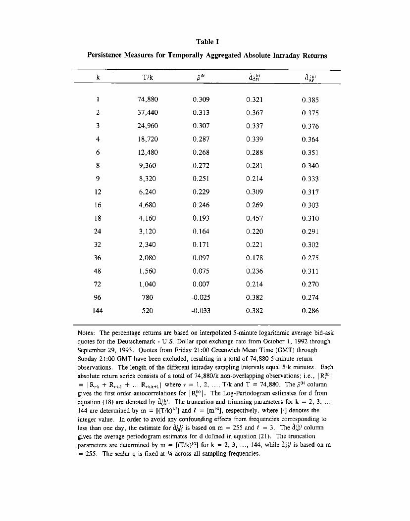
Table I

Persistence Measures for Temporally Aggregated Absolute Intraday Returns

1

2

3

4

6

8

9

12

16

18

24

32

36

48

72

96

144

74,880

37,440

24,960

18,720

12,480

9,360

8,320

6,240

4,680

4,160

3,120

2,340

2,080

1,560

1,040

780

520

0.309

0.313

0.307

0.287

0.268

0.272

0.251

0.229

0.246

0.193

0.164

0,171

0,097

0.075

0.007

-0.025

-0.033

0,321

0,367

0,337

0.339

0.288

0.281

0,214

0.309

0.269

0.457

0.220

0.221

0.178

0.236

0.214

0.382

0.382

0.385

0.375

0.376

0.364

0.351

0.340

0.333

0.317

0.303

0.310

0.291

0.302

0.275

0.311

0.270

0.274

0.286

Notes: The percentage returns are based on interpolated5-minutelogarithmicaveragebid-askquotes for the Deutschemark- U.S. Dollar spot exchangerate from October 1, 1992throughSeptember29, 1993. Quotes from Friday 21:00 GreenwichMean Time (GMT) throughSunday 21:00 GMT have been excluded, resulting in a total of 74,880 5-minute return

observations. The length of the different intraday sampling intervals equal 5 k minutes. Each

absolute return series consists of a total of 74,880/k non-overlapping observations; i.e., IR~kJI

= IR,., + R,.k., + ,.. K.k.k+,l where ~ = 1,2, . . . . T/k and T = 74,880. The D(k)COIU~

gives the first order autocorrelations for I~) 1. The Log-Periodogram estimates for d from

equation (18) me denoted by &~). The truncation and trimming parameters for k = 2, 3, ..,,

144 are determined by m = [(T/k) ID] and 1? = [ml’4], respectively, where [“] denotes the

integer value. In order to avoid any confounding effects from frequencies corresponding to

less than one day, the estimate for &!/ is based on m = 255 and f = 3. The d~j) column

gives the average periodogmn estimates for d defined in equation (21). The truncationparameters are determined by m = [(T/k) ’n] for k = 2, 3, . . .. 144, while ~,QJis based on m

= 255. The scalar q is fixed at % across all sampling frequencies.

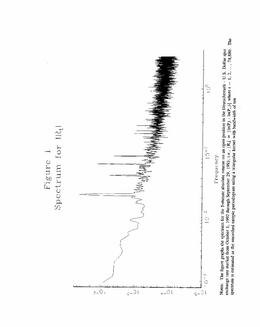
X--l

u“—-

\

(’

/

z_o 1 q_ol ~_Ol q-ol

z)

o-

—I

o

d

I3

)

3

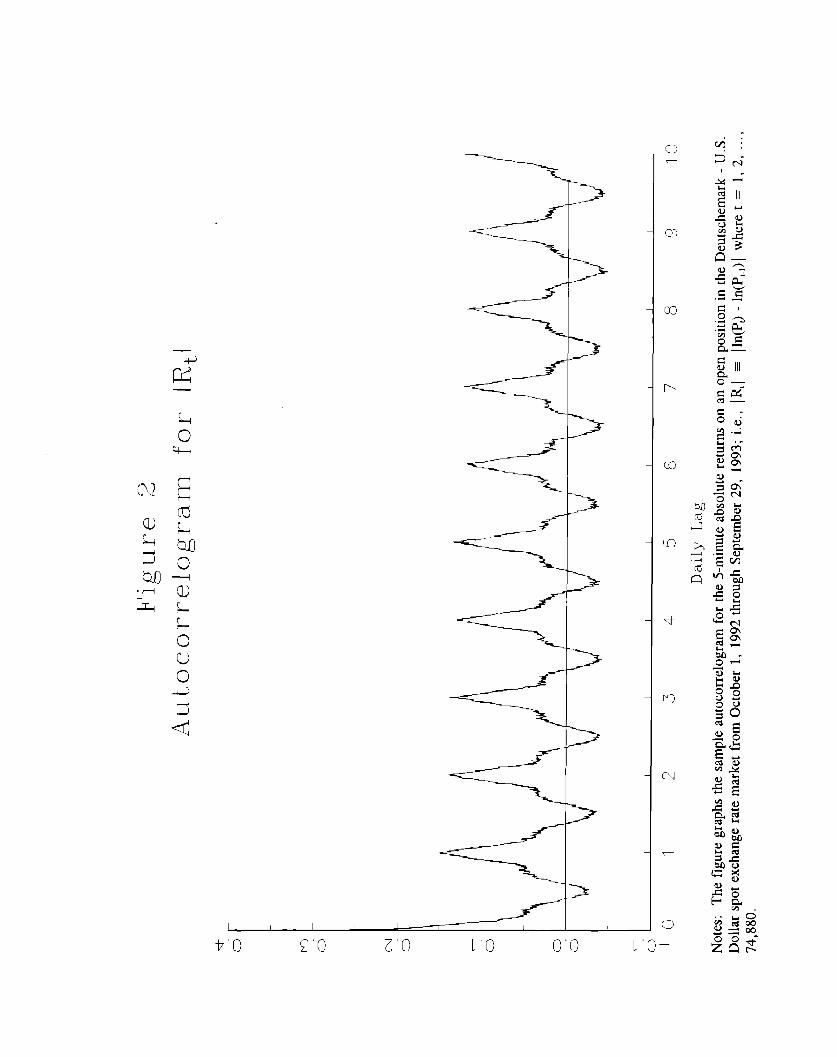
N

mlo

< .

C2

0

03

r--’

U2

m

+

w

N

a

ti”o so Z’o 1“0 0“0 ~“o–

“..\ ‘,\

‘.. \\

=-.

‘,<=---

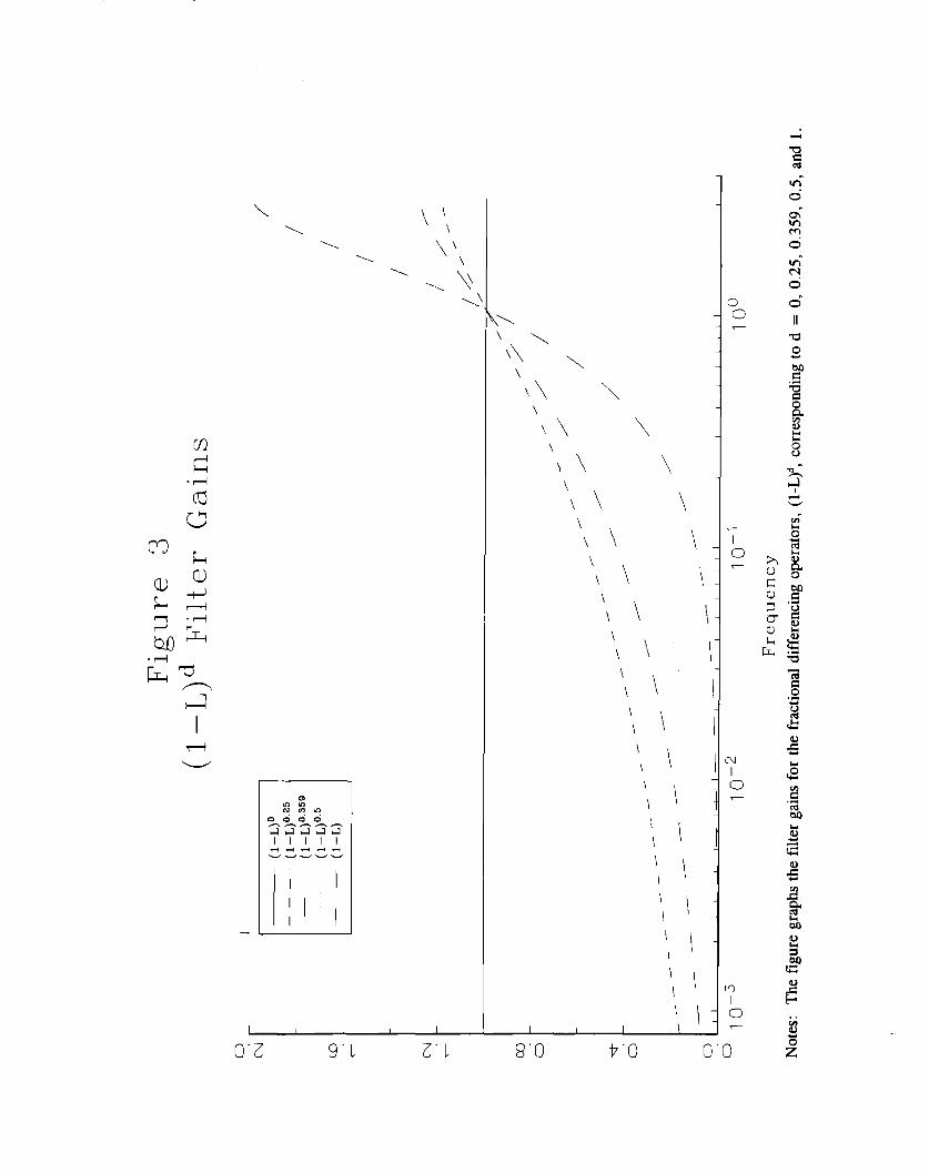
VI

I

1

o-z 9“1 z“ 1

\\\\

\\ \\

\\ \\

h \\\\\\\\\\

‘, \‘\ \‘, \

\

\

\.

\

\

‘\ \‘\ \‘\ \‘, \\\‘, \‘, I

‘, \‘\ \

I

I

I

,,:I ! I {

o0.

L).

N

L)

v

Io

8“0 17”o 0“0

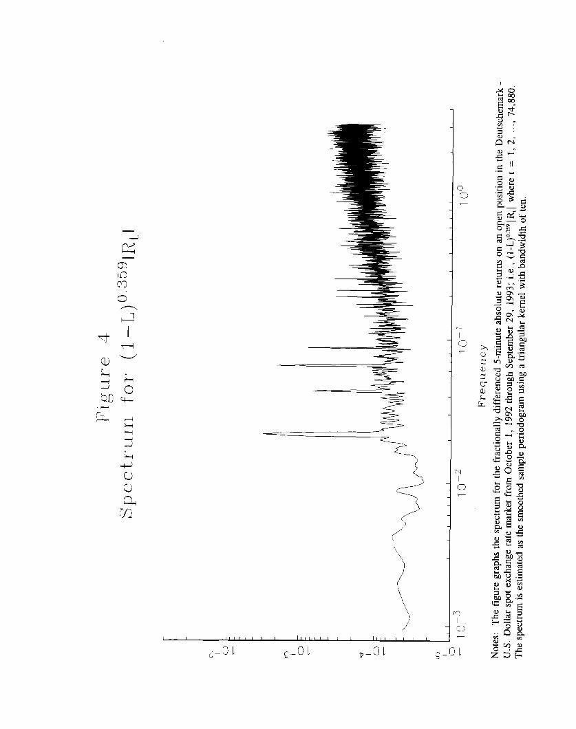
moz

4L

-#CJa)

.

—

—

/’

~-ol

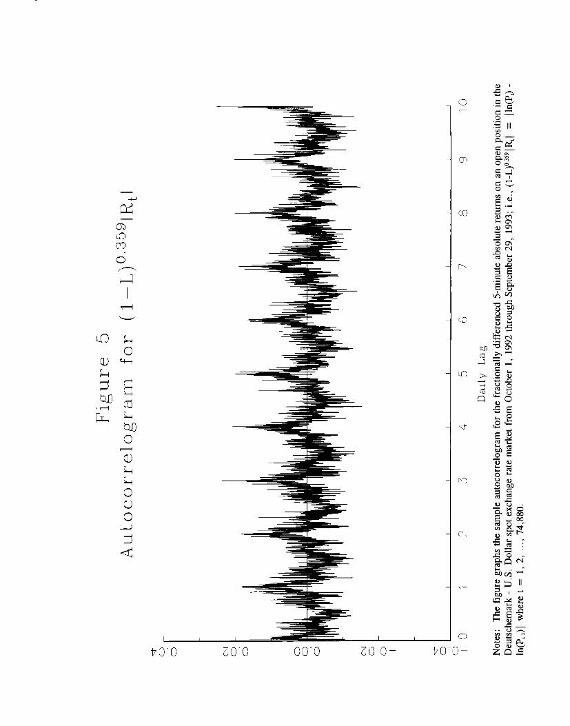
0

03l-nLr-3

—

>

0

L’ =lF—I7+

—

-

-

-—

——

❑

‘!

170”o 20”0 00”0 zo”o– +o”o–

+

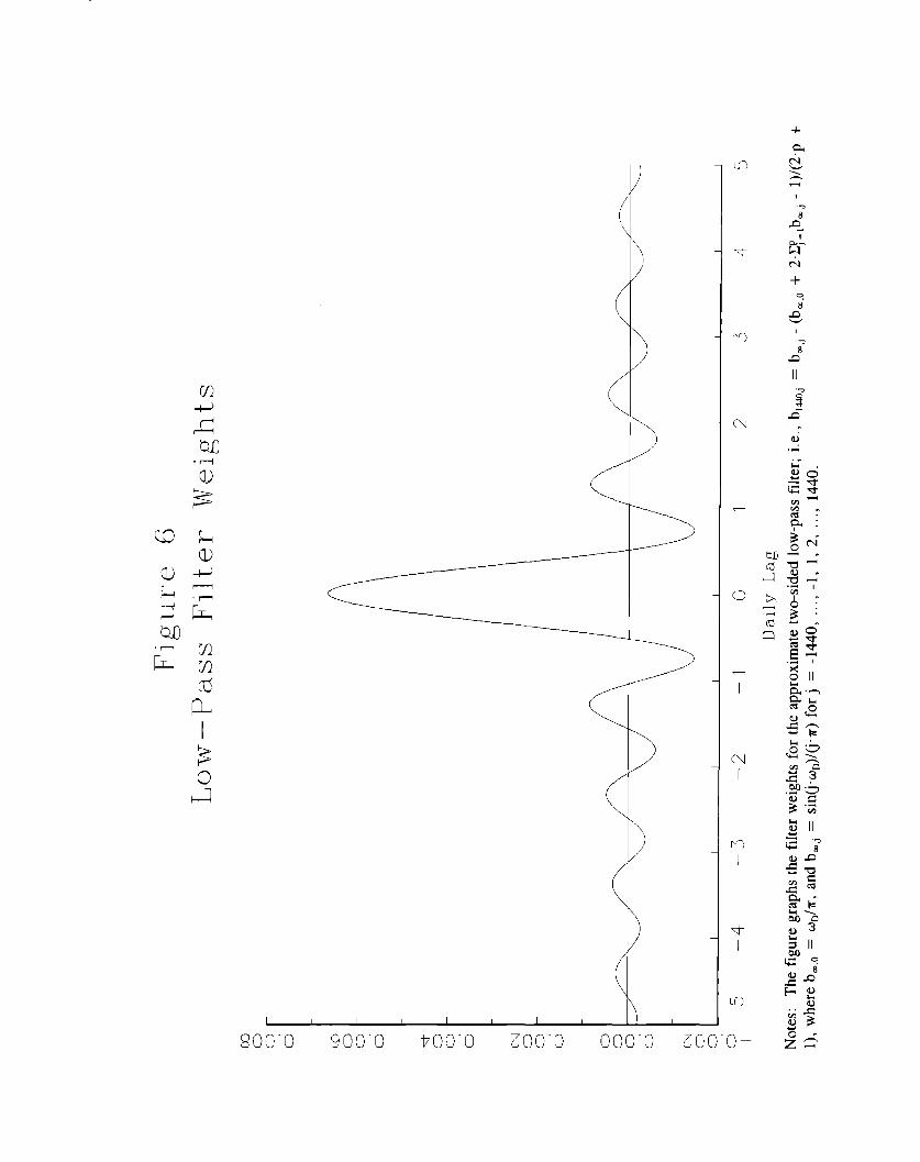
Q2

Q-II

c

—

<

>

>

(

I 1 I 1 I 1 I I

o

6!y.

c1

+

0-

D8

II

.

800”0 900’0 tioo-o 200”0 000”0 zoo”o -

— — — —— —.— —

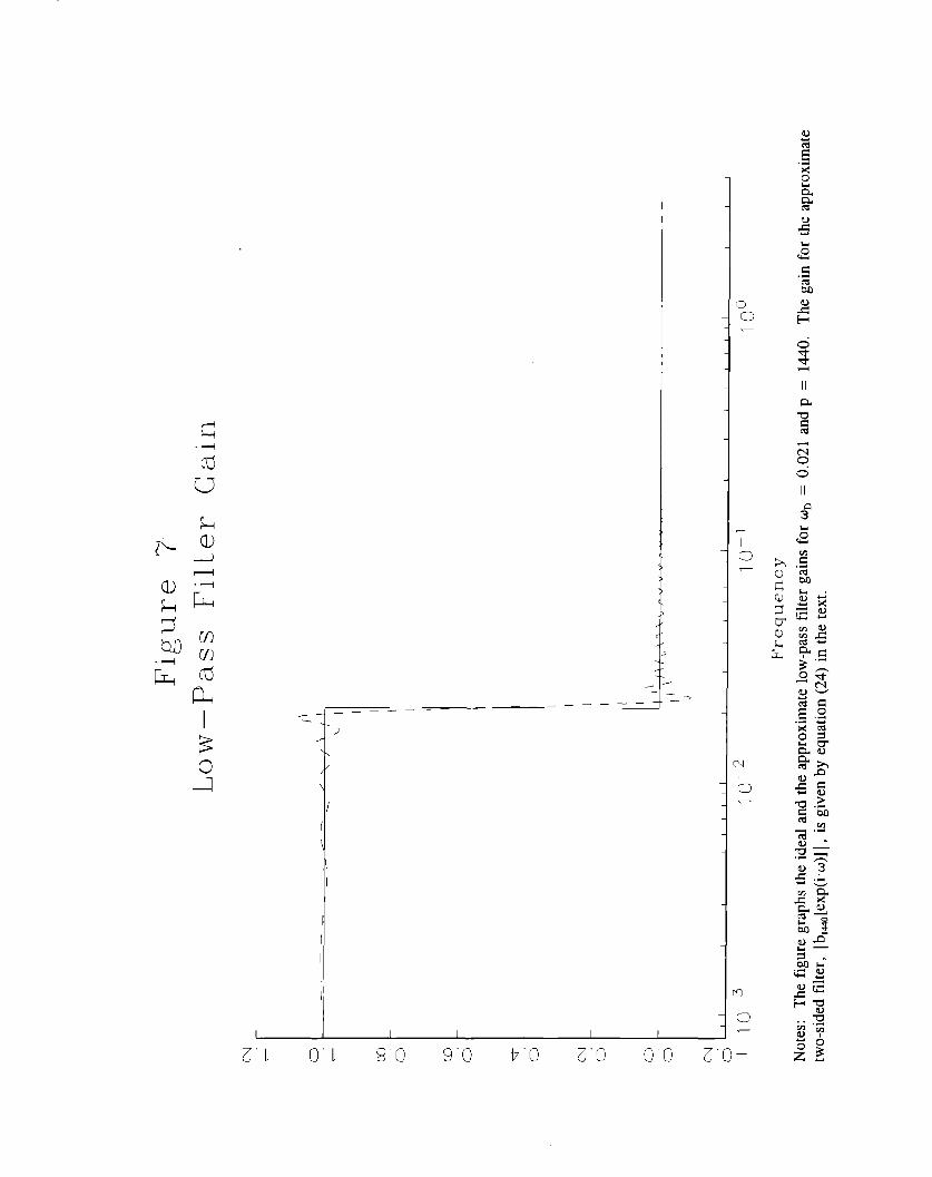
--J

,-

//

\

I

(\

\

I1

I(

I

I

II

Z“l 0“1 8“0 9“0 b-o Z“o 0“0 zo-

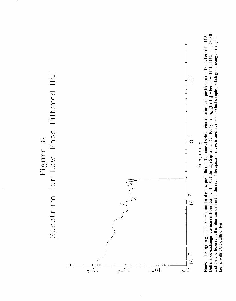
Eu)

cc:

ao

Io

N

o

‘n1

D

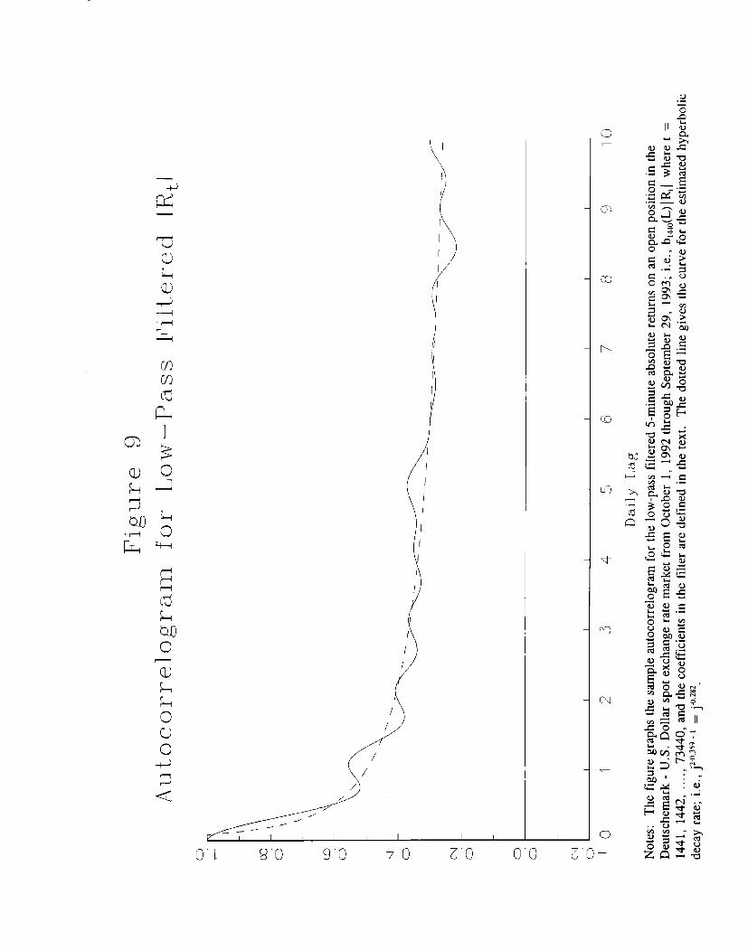
02

—4

—

-4

I

//l

f

/

/

/

I

I

/

0’1 8“0 9“0 $-0 2’0 0’0

0-

X2

r.

(’d

20: