Computer Networks : TCP Congestion Control1 TCP Congestion Control.
Upload
truongkhanhCategory
view
219download
0
Heterogeneous Congestion Control Protocols
Steven Low
CS, EEnetlab.CALTECH.edu
with A. Tang, J. Wang, D. Wei, CaltechM. Chiang, Princeton
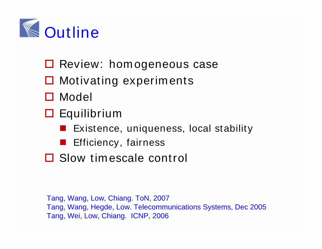
Outline
� Review: homogeneous case� Motivating experiments� Model� Equilibrium
� Existence, uniqueness, local stability� Efficiency, fairness
� Slow timescale control
Tang, Wang, Low, Chiang. ToN, 2007Tang, Wang, Hegde, Low. Telecommunications Systems, Dec 2005Tang, Wei, Low, Chiang. ICNP, 2006

Bibliography!!!
�Bibliography!!!
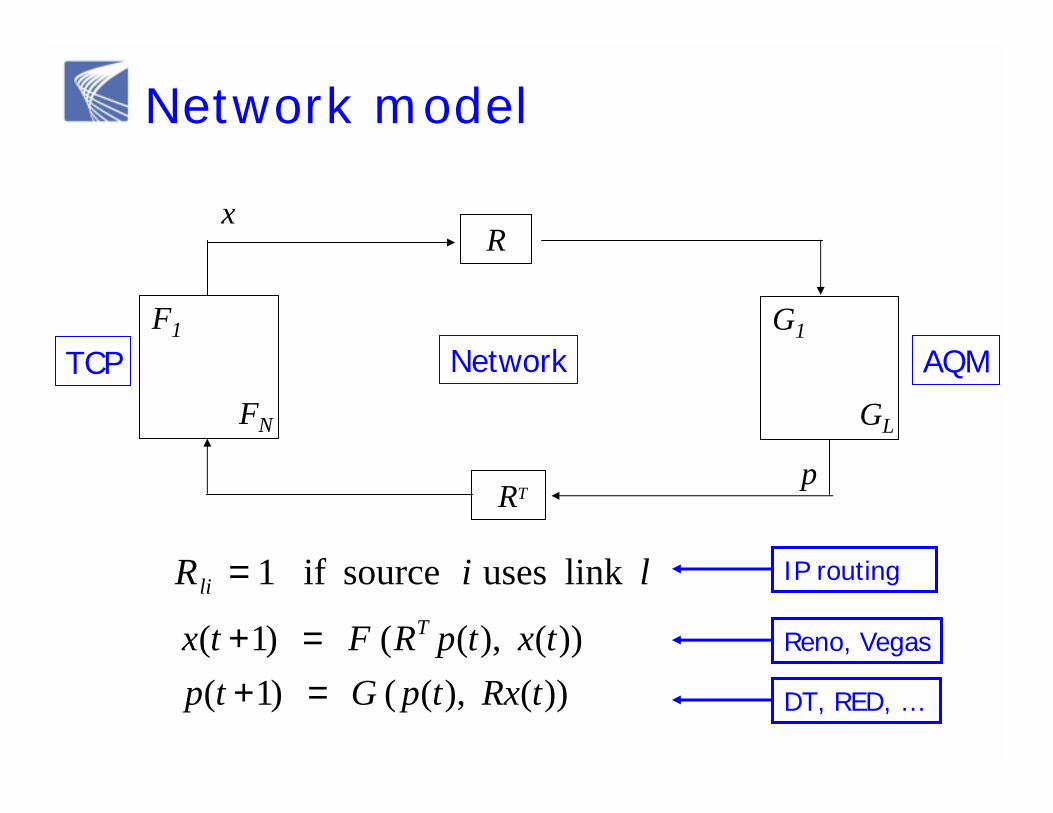
F1
FN
G1
GL
R
RT
TCP Network AQM
x y
q p
))( ),(( )1())( ),(( )1(
tRxtpGtptxtpRFtx T
=+=+ Reno, Vegas
DT, RED, …
liRli link uses source if 1= IP routing
Network model
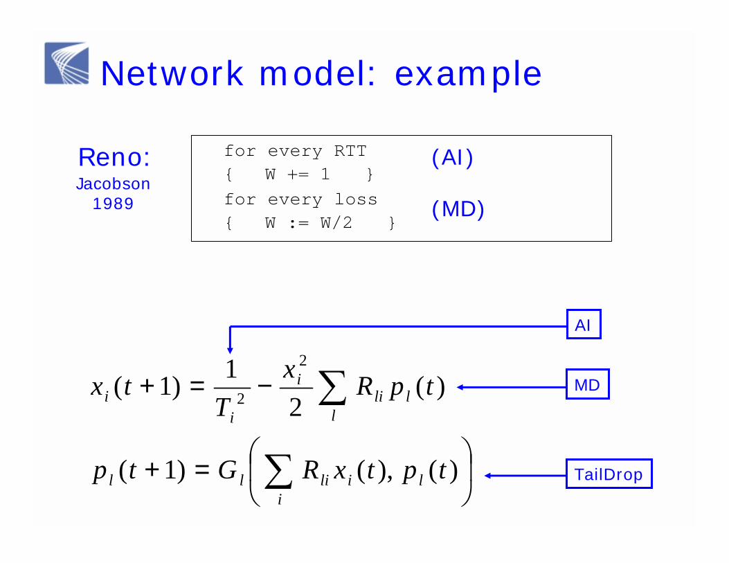
for every RTT
{ W += 1 }
for every loss
{ W := W/2 }
Reno: (AI)
(MD)Jacobson
1989
=+
−=+
∑
∑
ililill
llli
i
ii
tptxRGtp
tpRxT
tx
)(),()1(
)(2
1)1(2
2
AI
MD
TailDrop
Network model: example
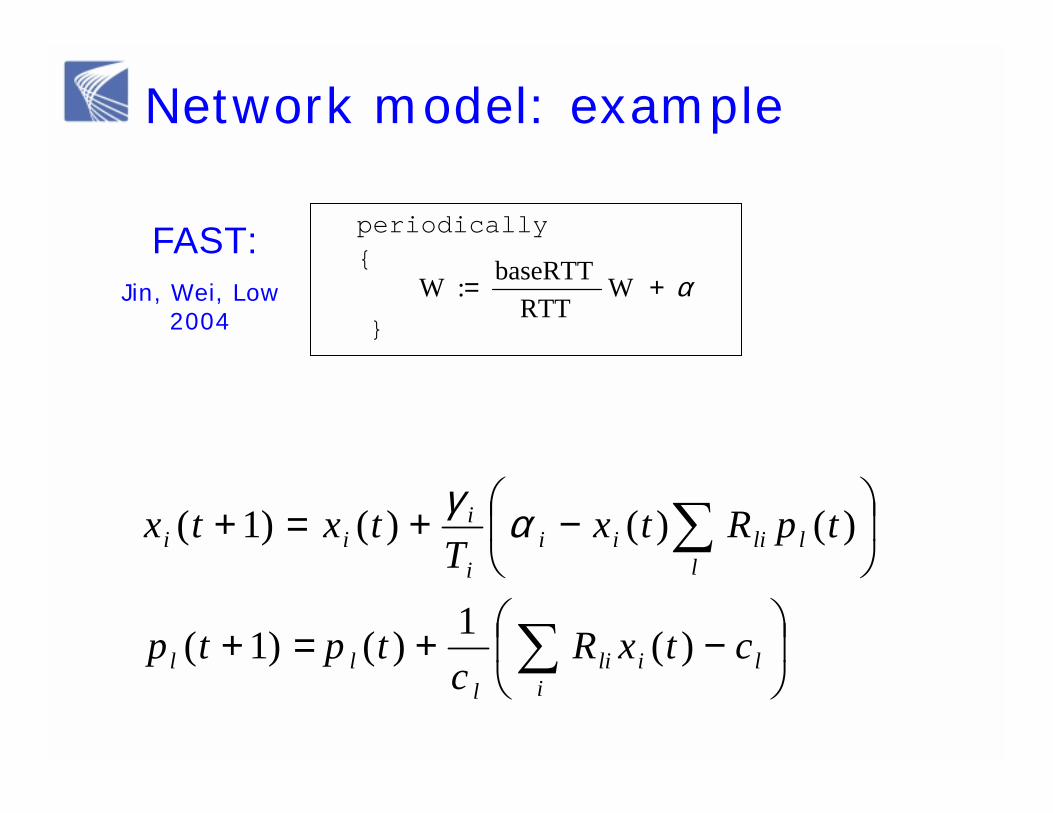
FAST:Jin, Wei, Low
2004α W
RTTbaseRTT :W +=
periodically
{
}
−+=+
−+=+
∑
∑
ilili
lll
llliii
i
iii
ctxRc
tptp
tpRtxT
txtx
)(1)()1(
)()()()1( αγ
Network model: example
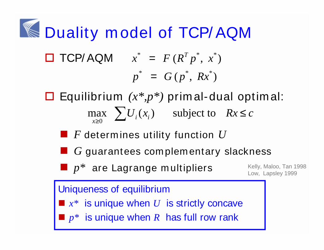
Duality model of TCP/AQM
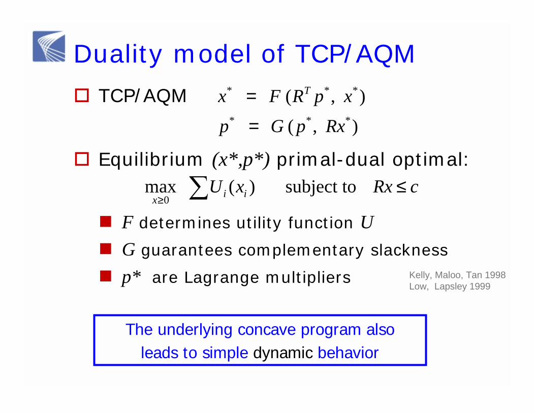
� TCP/AQM
� Equilibrium (x*,p*) primal-dual optimal:
� F determines utility function U� G guarantees complementary slackness
� p* are Lagrange multipliers
) ,( ) ,(
***
***
RxpGpxpRFx T
==
cRxxU iix≤∑≥
subject to )( max0
Uniqueness of equilibrium� x* is unique when U is strictly concave� p* is unique when R has full row rank
Kelly, Maloo, Tan 1998Low, Lapsley 1999
Duality model of TCP/AQM
� TCP/AQM
� Equilibrium (x*,p*) primal-dual optimal:
� F determines utility function U� G guarantees complementary slackness
� p* are Lagrange multipliers
) ,( ) ,(
***
***
RxpGpxpRFx T
==
cRxxU iix≤∑≥
subject to )( max0
Kelly, Maloo, Tan 1998Low, Lapsley 1999
The underlying concave program also leads to simple dynamic behavior
Duality model of TCP/AQM
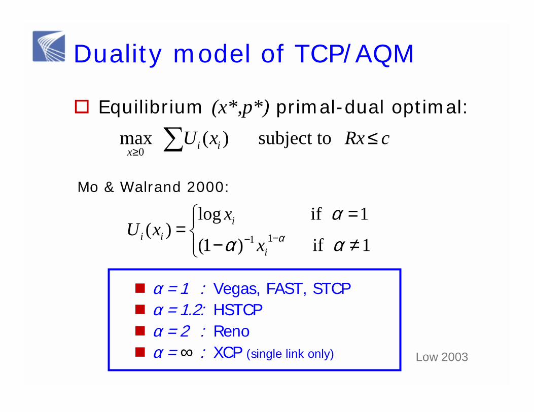
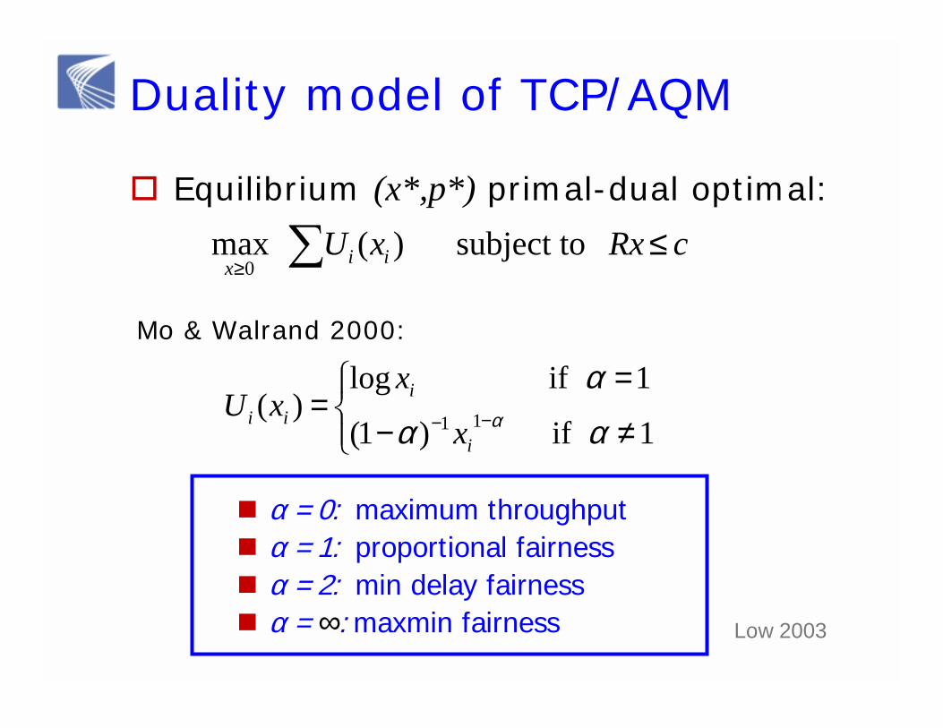
� Equilibrium (x*,p*) primal-dual optimal:
cRxxU iix≤∑≥
subject to )( max0
Mo & Walrand 2000:
≠−
== −− 1 if )1(
1 if log)( 11 αα
αα
i
iii x
xxU
� α = 1 : Vegas, FAST, STCP � α = 1.2: HSTCP� α = 2 : Reno� α = : XCP (single link only) ∞ Low 2003
Duality model of TCP/AQM
� Equilibrium (x*,p*) primal-dual optimal:
cRxxU iix≤∑≥
subject to )( max0
Mo & Walrand 2000:
≠−
== −− 1 if )1(
1 if log)( 11 αα
αα
i
iii x
xxU
Low 2003
� α = 0: maximum throughput � α = 1: proportional fairness � α = 2: min delay fairness � α = : maxmin fairness ∞
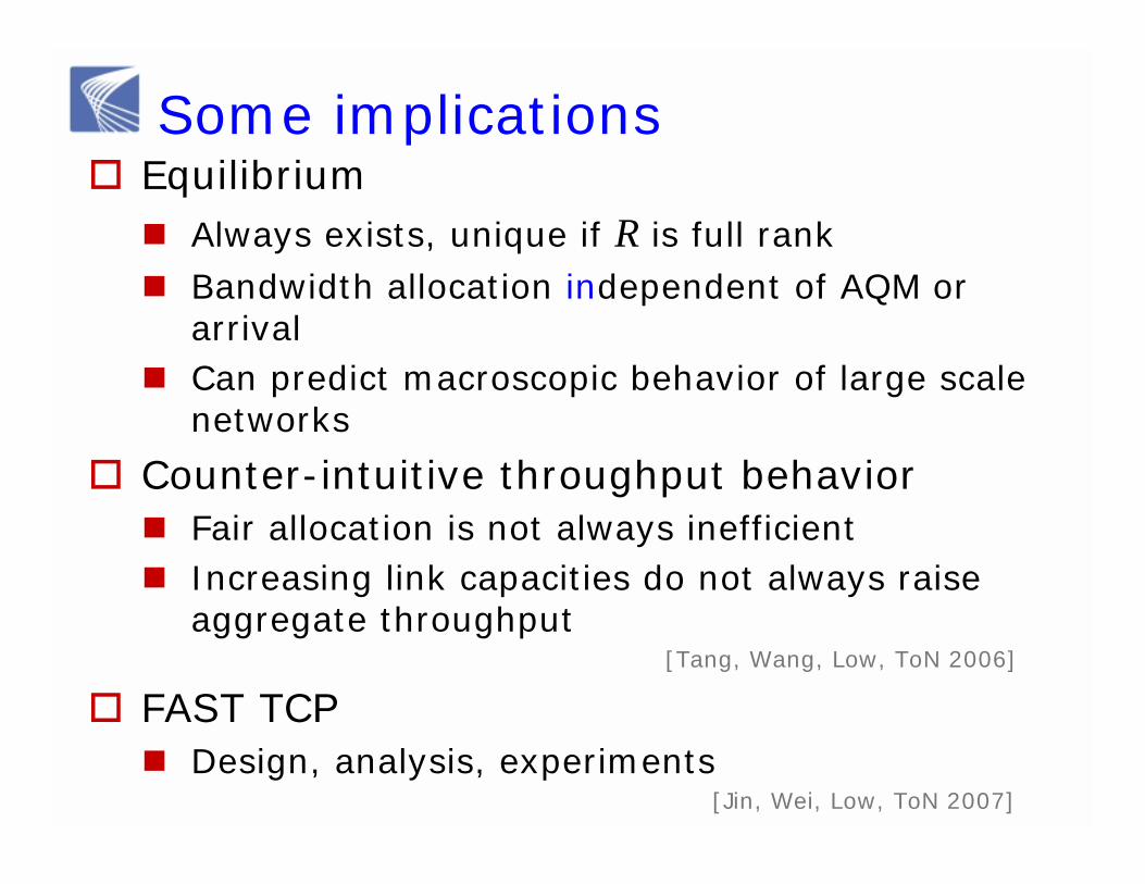
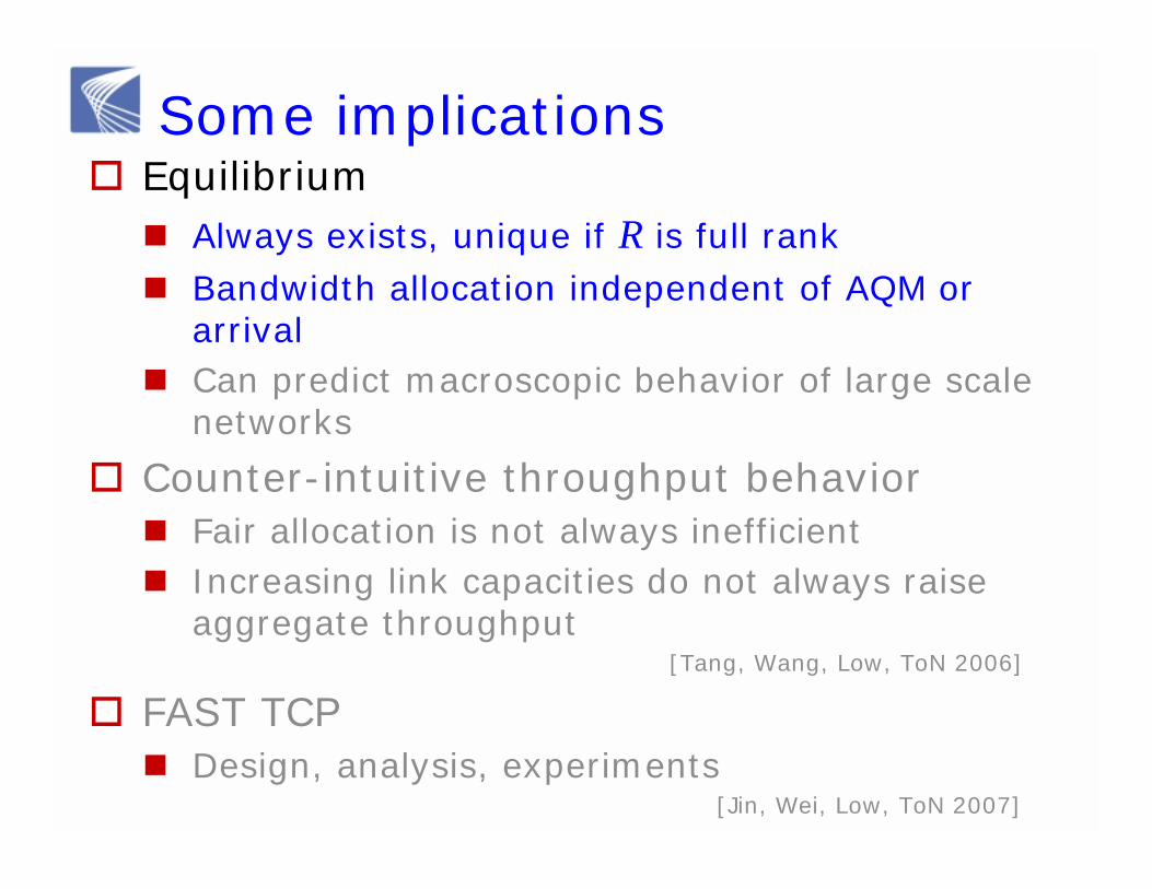
Some implications� Equilibrium
� Always exists, unique if R is full rank� Bandwidth allocation independent of AQM or
arrival� Can predict macroscopic behavior of large scale
networks
� Counter-intuitive throughput behavior� Fair allocation is not always inefficient � Increasing link capacities do not always raise
aggregate throughput[Tang, Wang, Low, ToN 2006]
� FAST TCP� Design, analysis, experiments
[Jin, Wei, Low, ToN 2007]
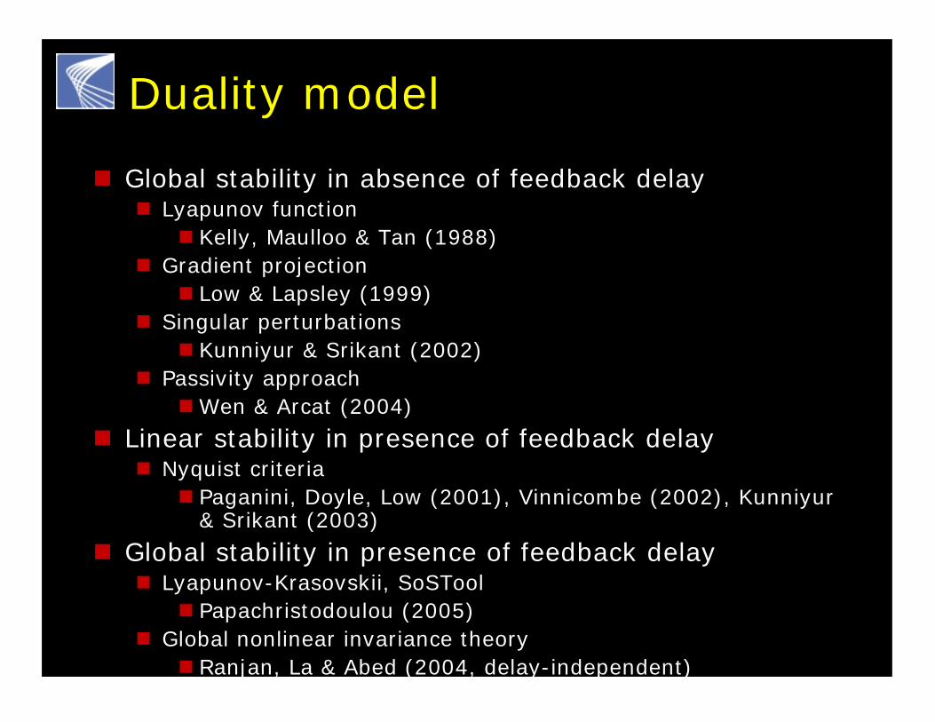
Duality model
� Global stability in absence of feedback delay� Lyapunov function
� Kelly, Maulloo & Tan (1988)� Gradient projection
� Low & Lapsley (1999)� Singular perturbations
� Kunniyur & Srikant (2002)� Passivity approach
� Wen & Arcat (2004)
� Linear stability in presence of feedback delay� Nyquist criteria
� Paganini, Doyle, Low (2001), Vinnicombe (2002), Kunniyur& Srikant (2003)
� Global stability in presence of feedback delay� Lyapunov-Krasovskii, SoSTool
� Papachristodoulou (2005)� Global nonlinear invariance theory
� Ranjan, La & Abed (2004, delay-independent)
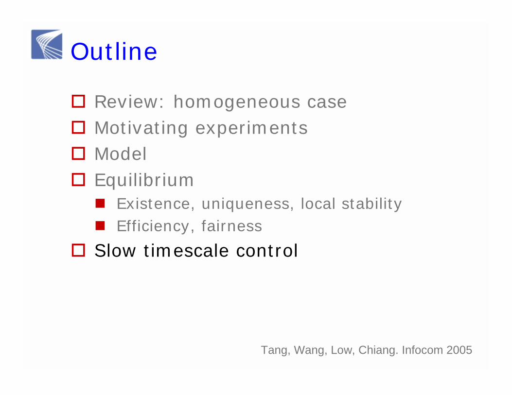
Outline
� Review: homogeneous case� Motivating experiments� Model� Equilibrium
� Existence, uniqueness, local stability� Efficiency, fairness
� Slow timescale control

The world is heterogeneous…
� Linux 2.6.13 allows users to choose congestion control algorithms
� Many protocol proposals� Loss- based: Reno and a large number of
variants� Delay- based: CARD (1989), DUAL (1992), Vegas
(1995), FAST (2004), …� ECN: RED (1993), REM (2001), PI (2002), AVQ
(2003), …� Explicit feedback: MaxNet (2002), XCP (2002),
RCP (2005), …
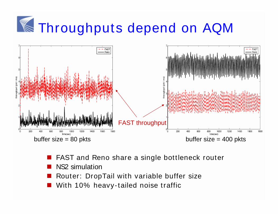
Throughputs depend on AQM
� FAST and Reno share a single bottleneck router� NS2 simulation� Router: DropTail with variable buffer size � With 10% heavy-tailed noise traffic
FAST throughput
buffer size = 80 pkts buffer size = 400 pkts

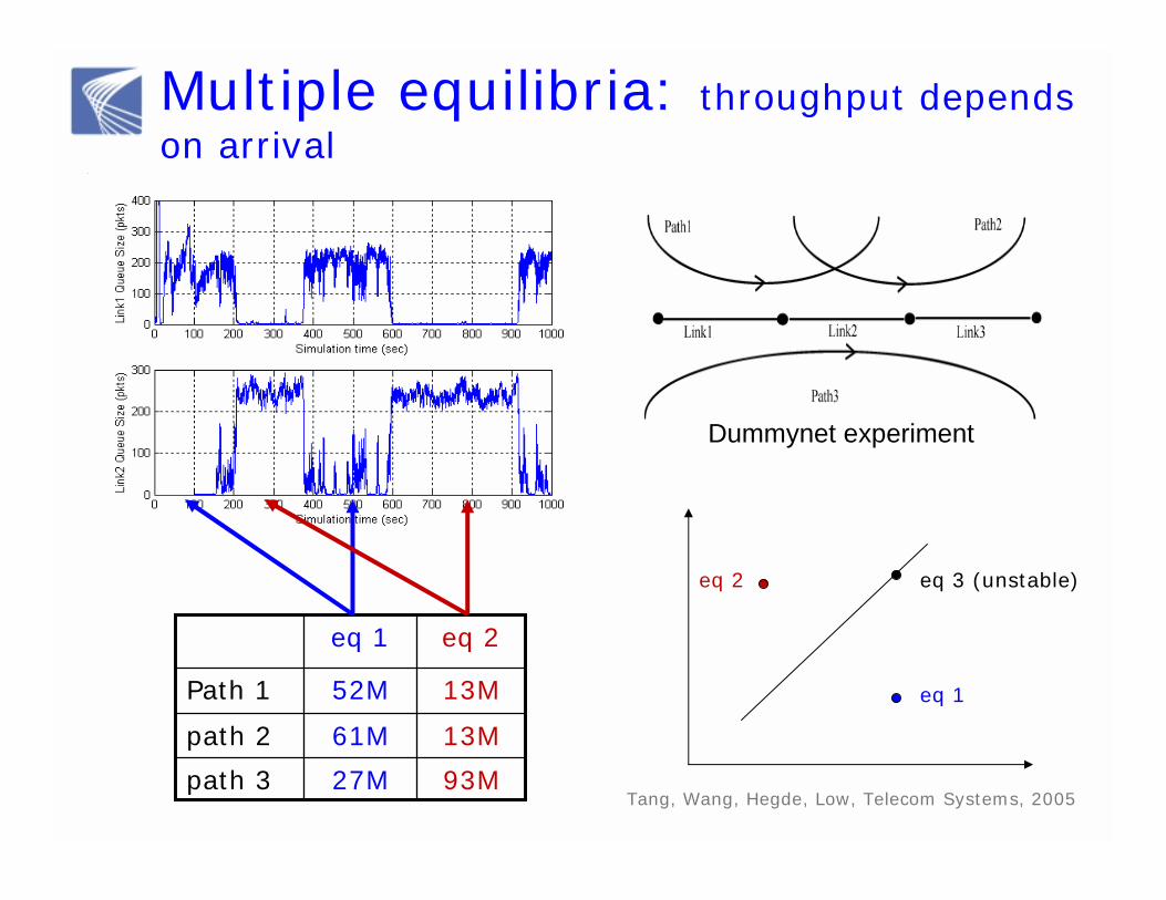
Multiple equilibria: throughput depends on arrival
13M61Mpath 2
93M27Mpath 3
13M52MPath 1
eq 2eq 1
eq 1
eq 2
Tang, Wang, Hegde, Low, Telecom Systems, 2005
Dummynet experiment
13M61Mpath 2
93M27Mpath 3
13M52MPath 1
eq 2eq 1
Tang, Wang, Hegde, Low, Telecom Systems, 2005
eq 1
eq 2 eq 3 (unstable)
Dummynet experiment
Multiple equilibria: throughput depends on arrival
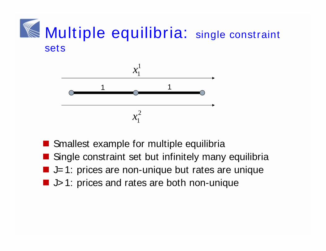
Multiple equilibria: single constraint sets
1 1
11x
21x
� Smallest example for multiple equilibria� Single constraint set but infinitely many equilibria� J=1: prices are non-unique but rates are unique� J>1: prices and rates are both non-unique
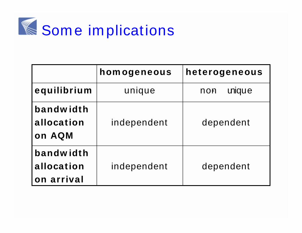
Some implications
dependentindependentbandwidthallocationon arrival
dependentindependentbandwidthallocation on AQM
non- uniqueuniqueequilibrium
heterogeneoushomogeneous
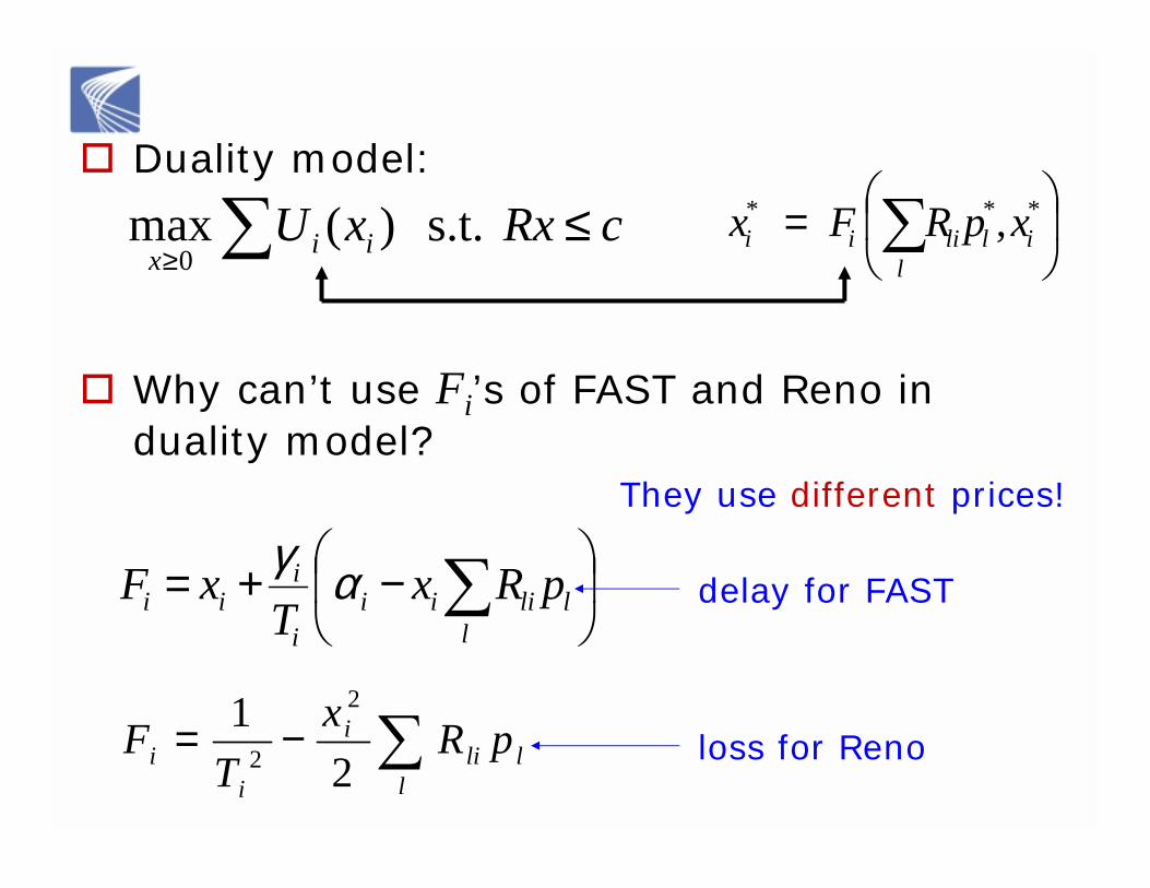
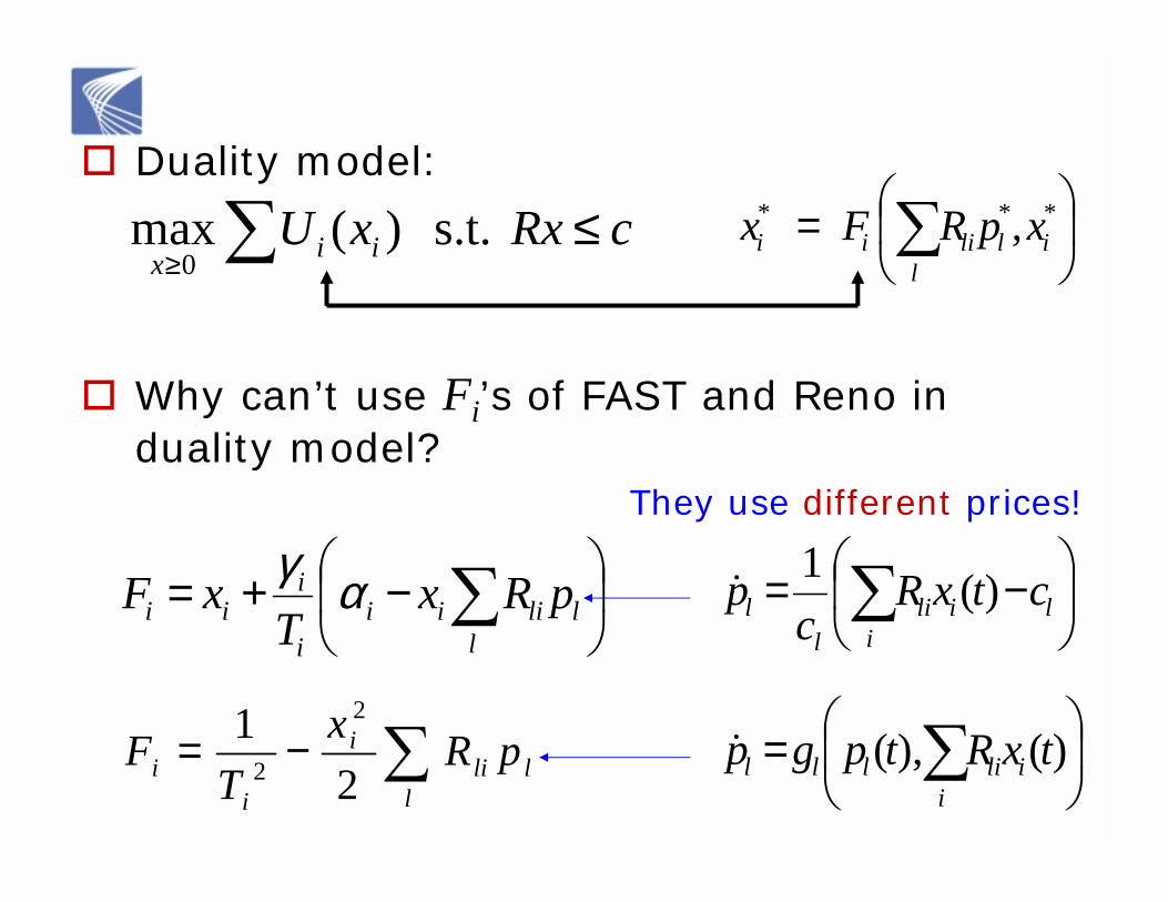
� Duality model:
, ***
= ∑l
illiii xpRFxcRxxU iix≤∑≥
s.t. )( max0
−+= ∑l
lliiii
iii pRx
TxF αγ
� Why can’t use Fi’s of FAST and Reno in duality model?
∑−=l
llii
ii pRx
TF
21 2
2
delay for FAST
loss for Reno
They use different prices!
� Duality model:
, ***
= ∑l
illiii xpRFxcRxxU iix≤∑≥
s.t. )( max0
−+= ∑l
lliiii
iii pRx
TxF αγ
� Why can’t use Fi’s of FAST and Reno in duality model?
∑−=l
llii
ii pRx
TF
21 2
2
They use different prices!
−= ∑i
lilil
l ctxRc
p )(1D
= ∑i
ililll txRtpgp )(),(D
F1
FN
G1
GL
R
RT
TCP Network AQM
x y
q p
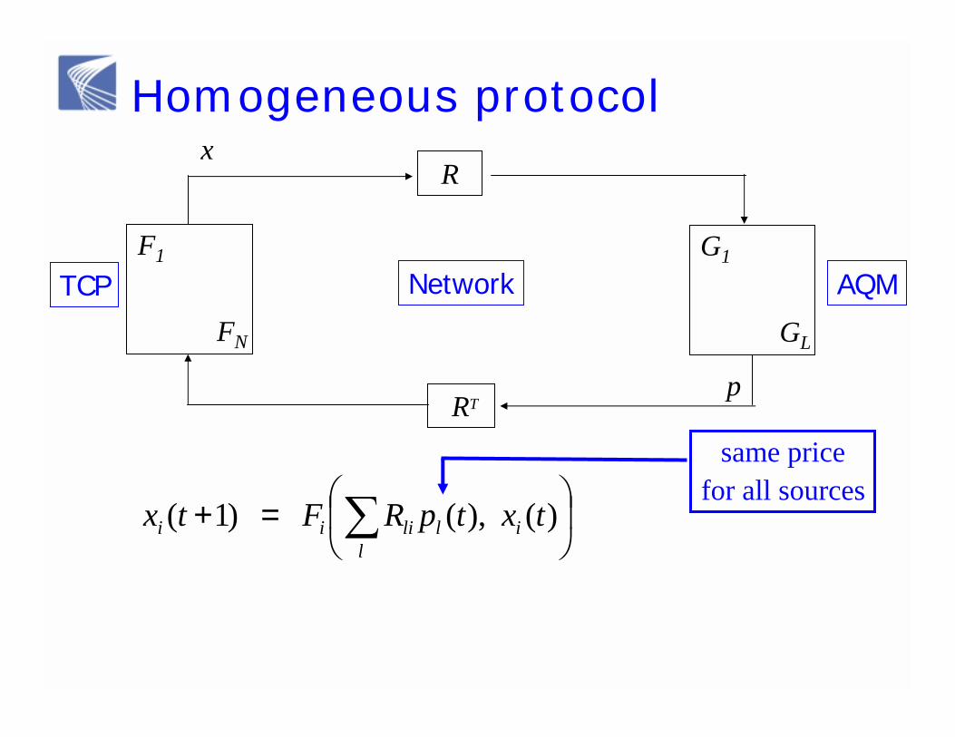
Homogeneous protocol
( )
=+
=+
∑
∑
)( ,)( )1(
)( ,)( )1(
txtpmRFtx
txtpRFtx
ji
ll
jlli
ji
ji
il
lliii
same pricefor all sources
F1
FN
G1
GL
R
RT
TCP Network AQM
x y
q p
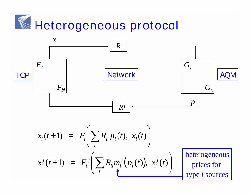
Heterogeneous protocol
( )
=+
=+
∑
∑
)( ,)( )1(
)( ,)( )1(
txtpmRFtx
txtpRFtx
ji
ll
jlli
ji
ji
il
lliii
heterogeneousprices for
type j sources
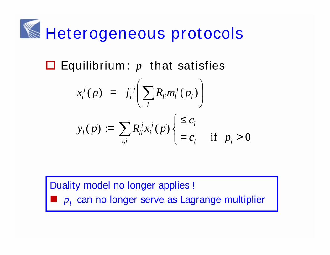
Heterogeneous protocols
� Equilibrium: p that satisfies
∑
∑
>=≤
=
=
i,j ll
lji
jlil
ll
jlli
ji
ji
pcc
pxRpy
pmRfpx
0 if
)( : )(
)( )(
Duality model no longer applies !� pl can no longer serve as Lagrange multiplier
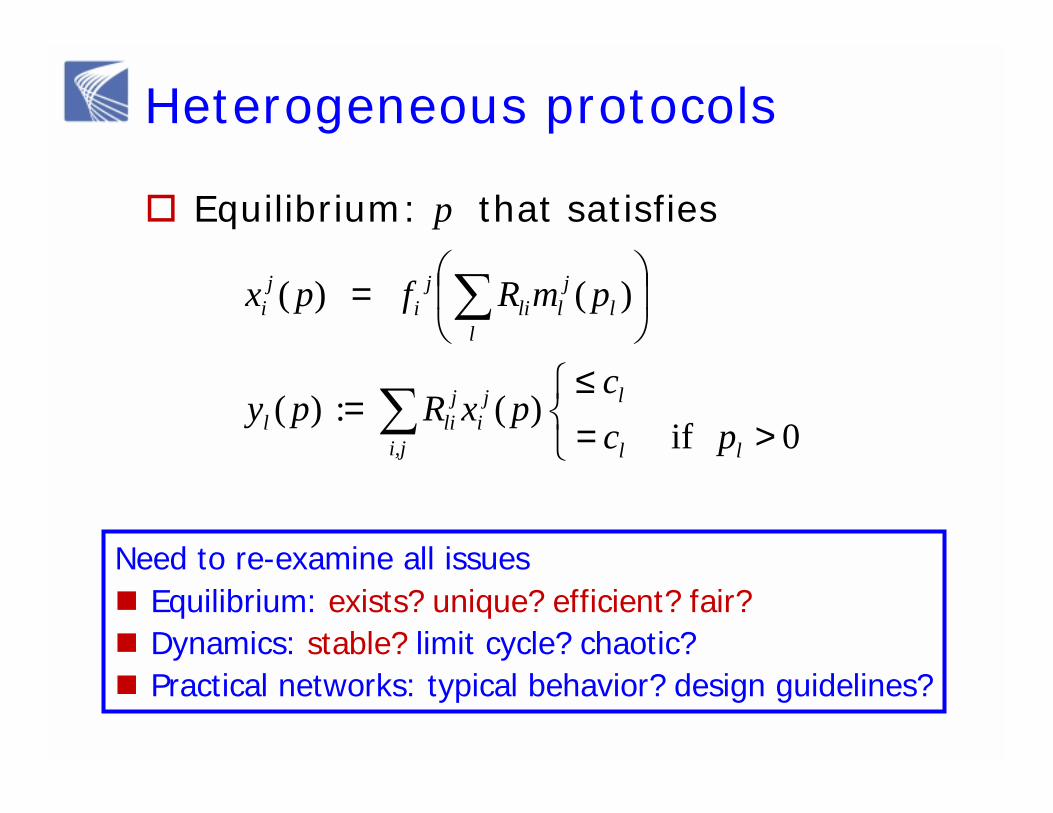
Heterogeneous protocols
� Equilibrium: p that satisfies
∑
∑
>=≤
=
=
i,j ll
lji
jlil
ll
jlli
ji
ji
pcc
pxRpy
pmRfpx
0 if
)( : )(
)( )(
Need to re-examine all issues� Equilibrium: exists? unique? efficient? fair?� Dynamics: stable? limit cycle? chaotic?� Practical networks: typical behavior? design guidelines?
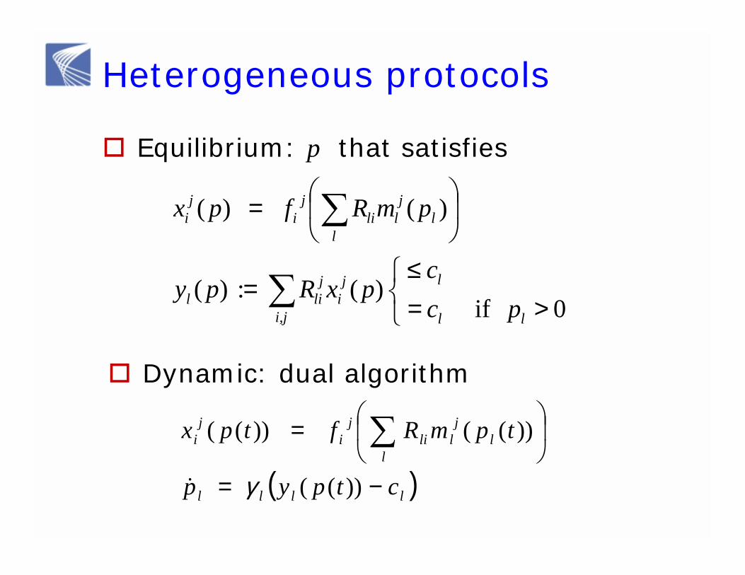
Heterogeneous protocols
� Equilibrium: p that satisfies
∑
∑
>=≤
=
=
i,j ll
lji
jlil
ll
jlli
ji
ji
pcc
pxRpy
pmRfpx
0 if
)( : )(
)( )(
� Dynamic: dual algorithm
( )llll
ll
jlli
ji
ji
ctpyp
tpmRftpx
−=
= ∑
))((
))(( ))((
γC
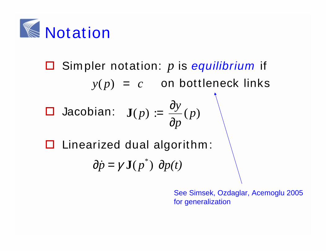
Notation
� Simpler notation: p is equilibrium ifon bottleneck links
� Jacobian:
� Linearized dual algorithm:
cpy )( =
)( : )( ppyp
∂∂=J
p(t)pp ∂=∂ )( *JγC
See Simsek, Ozdaglar, Acemoglu 2005for generalization
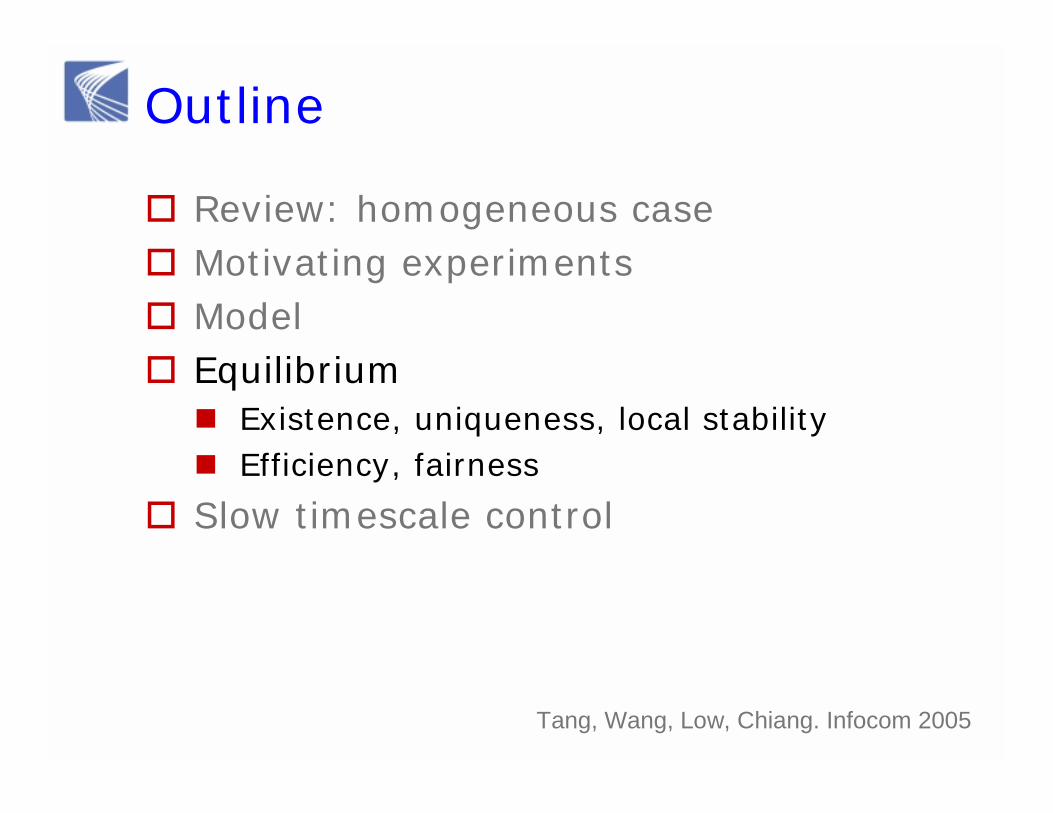
Outline
� Review: homogeneous case� Motivating experiments� Model� Equilibrium
� Existence, uniqueness, local stability� Efficiency, fairness
� Slow timescale control
Tang, Wang, Low, Chiang. Infocom 2005
Existence
Theorem
Equilibrium p exists, despite lack of underlying utility maximization
� Generally non-unique� There are networks with unique bottleneck
set but infinitely many equilibria� There are networks with multiple bottleneck
set each with a unique (but distinct) equilibrium

Regular networks
Definition
A regular network is a tuple (R, c, m, U) for which all equilibria p are locally unique, i.e.,
Theorem� Almost all networks are regular� A regular network has finitely many and
odd number of equilibria (e.g. 1)
0 )(det : )(det ≠∂∂= ppypJ
Regular networks
Proof idea:� Sard’s Theorem: critical value of a
continuously differentiable function over open set has measure zero
� Apply to y(p) = c on each bottleneck set � regularity
� Compact equilibrium set � finiteness
Regular networks
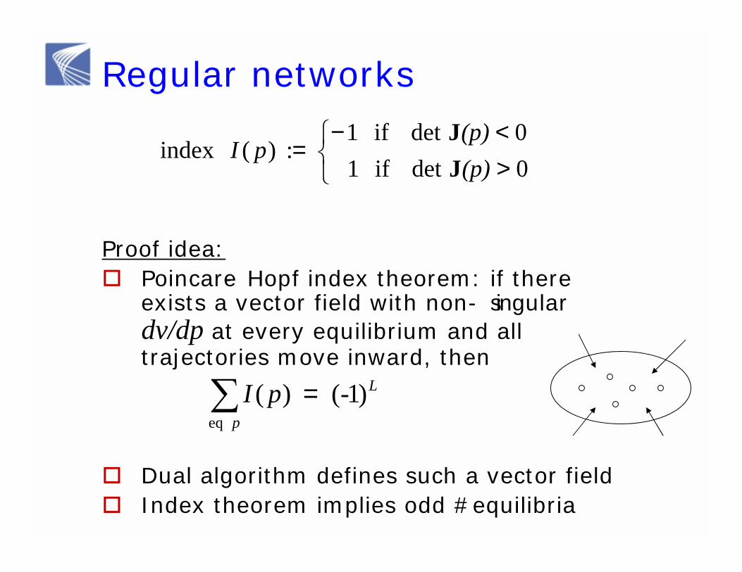
Proof idea:� Poincare- Hopf index theorem: if there
exists a vector field with non- singular dv/dp at every equilibrium and all trajectories move inward, then
� Dual algorithm defines such a vector field� Index theorem implies odd #equilibria
><−
=0det if 1 0det if 1
: )(index (p)(p)
pIJJ
L
p- pI )1( )(
eq
=∑
Global uniqueness
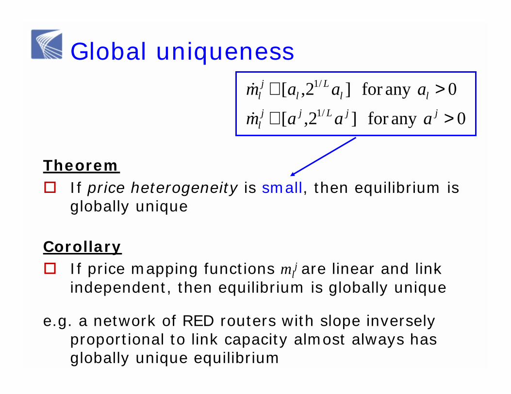
Corollary� If price mapping functions ml
j are linear and link-independent, then equilibrium is globally unique
e.g. a network of RED routers with slope inversely proportional to link capacity almost always has globally unique equilibrium
Theorem� If price heterogeneity is small, then equilibrium is
globally unique
0any for ]2,[
0any for ]2,[/1
/1
>∈
>∈jjLjj
l
llL
lj
l
aaamaaam
D
D
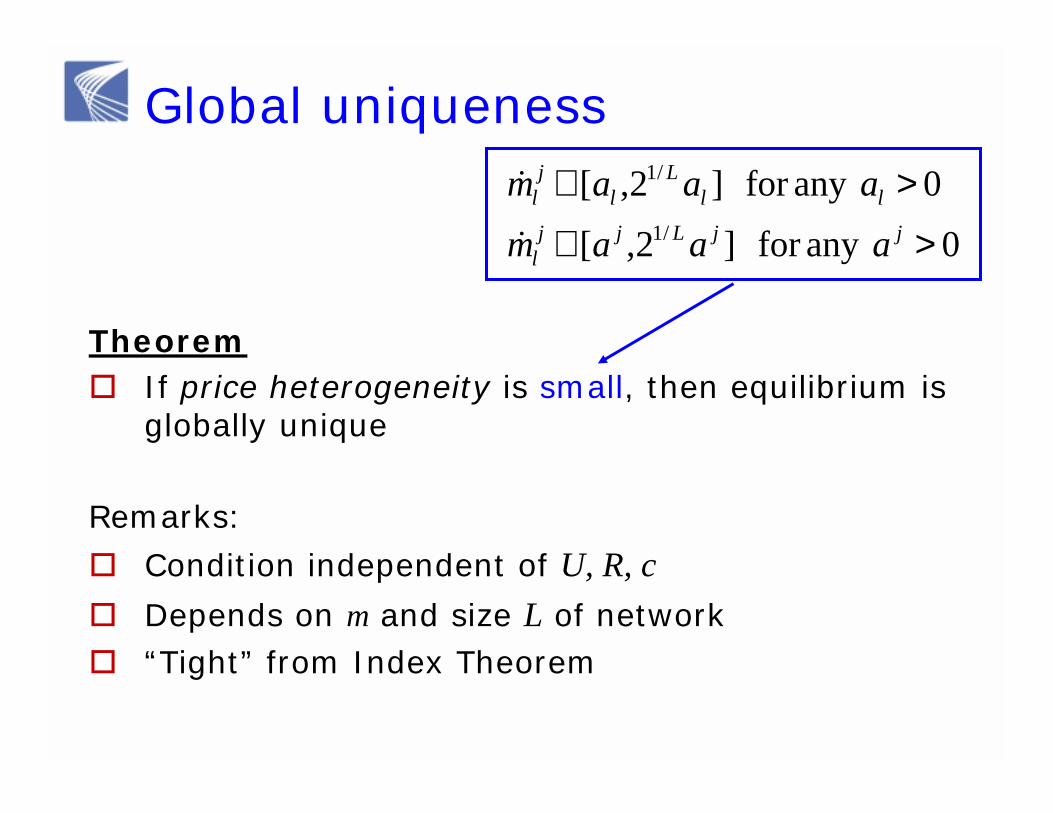
Global uniqueness
Remarks:
� Condition independent of U, R, c� Depends on m and size L of network � “Tight” from Index Theorem
Theorem� If price heterogeneity is small, then equilibrium is
globally unique
0any for ]2,[
0any for ]2,[/1
/1
>∈
>∈jjLjj
l
llL
lj
l
aaamaaam
D
D

Local stability:`uniqueness’ � stability
Theorem� If price heterogeneity is small, then the unique
equilibrium p is locally stable
0any for ]2,[
0any for ]2,[/1
/1
>∈
>∈jjLjj
l
llL
lj
l
aaamaaam
D
D
p(t)pp δγδ )( *J=DLinearized dual algorithm:
Equilibrium p is locally stable if
( ) 0 )( Re <pJλ
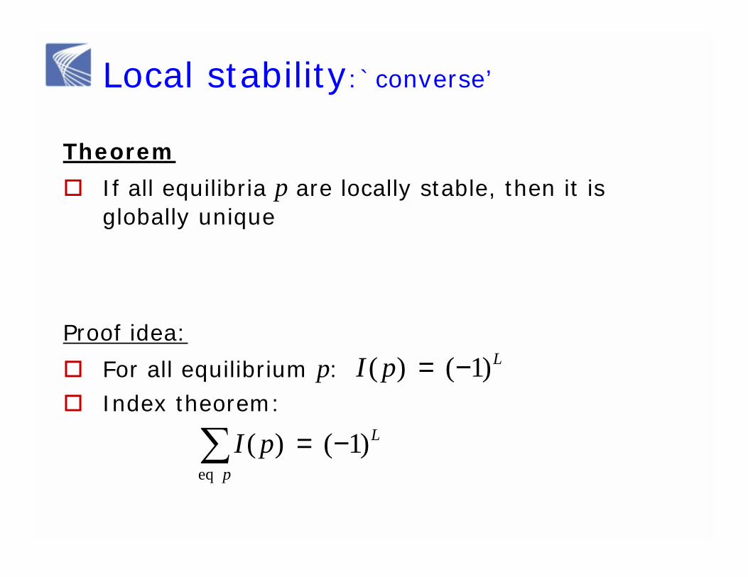
Local stability:`converse’
Theorem
� If all equilibria p are locally stable, then it is globally unique
LpI )1( )( −=Proof idea:
� For all equilibrium p:� Index theorem:
L
ppI )1( )(
eq−=∑

Outline
� Review: homogeneous case� Motivating experiments� Model� Equilibrium
� Existence, uniqueness, local stability� Efficiency, fairness
� Slow timescale control
Tang, Wang, Low, Chiang. Infocom 2005
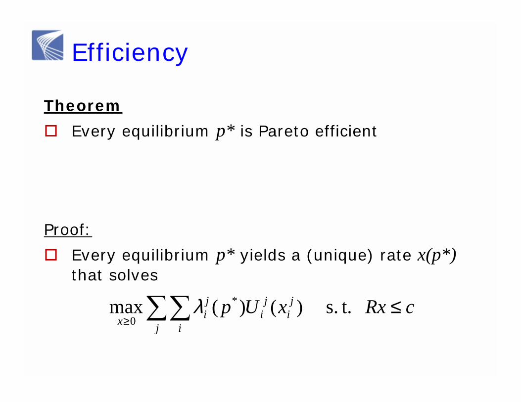
Efficiency
Theorem
� Every equilibrium p* is Pareto efficient
Proof:
� Every equilibrium p* yields a (unique) rate x(p*)that solves
∑∑ ≤≥ j i
ji
ji
jix
cRxxUp t.s. )()(max *
0λ
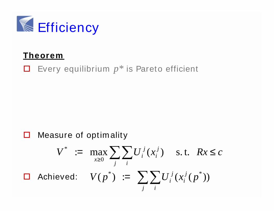
Efficiency
Theorem
� Every equilibrium p* is Pareto efficient
� Measure of optimality
� Achieved:
∑∑ ≤=≥ j i
ji
jix
cRxxUV t.s. )(max : 0
*
∑∑=j i
ji
ji pxUpV ))(( : )( **
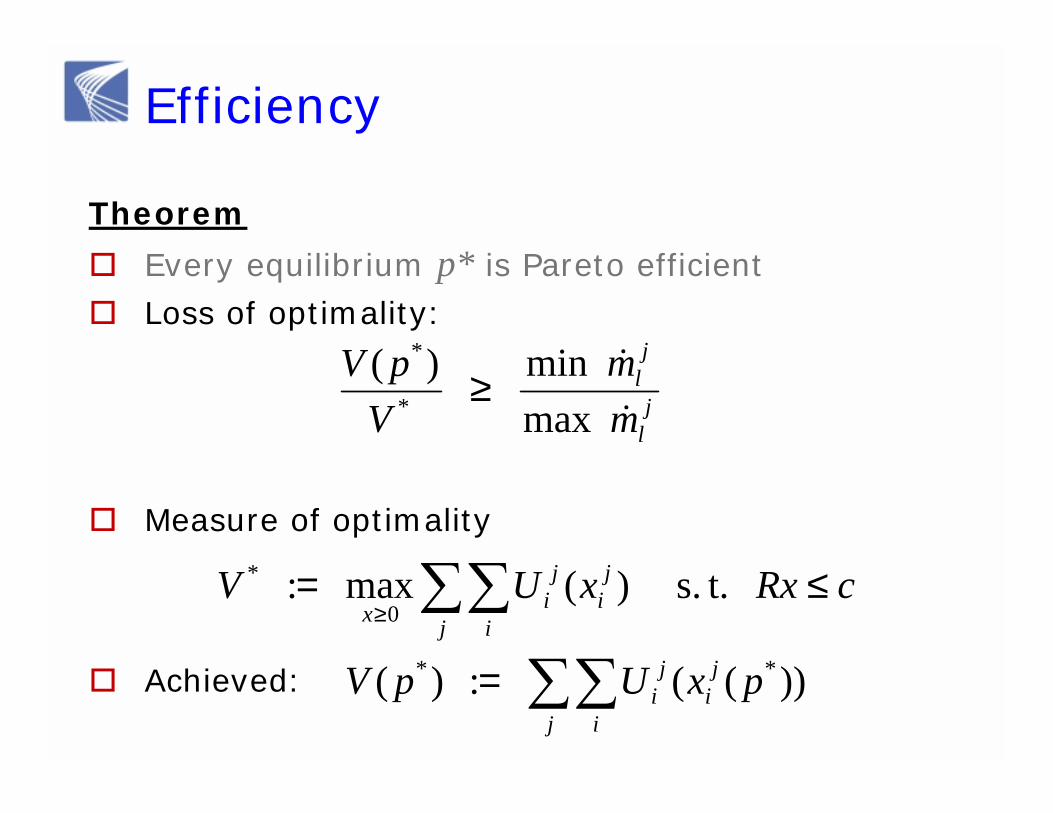
Efficiency
Theorem
� Every equilibrium p* is Pareto efficient� Loss of optimality:
� Measure of optimality
� Achieved:
∑∑ ≤=≥ j i
ji
jix
cRxxUV t.s. )(max : 0
*
∑∑=j i
ji
ji pxUpV ))(( : )( **
jl
jl
mm
VpV
D
D
max min )(
*
*
≥
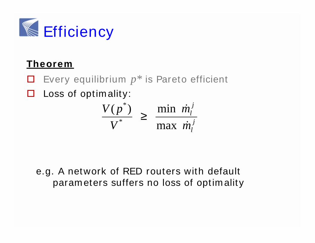
Efficiency
Theorem
� Every equilibrium p* is Pareto efficient� Loss of optimality:
e.g. A network of RED routers with default parameters suffers no loss of optimality
jl
jl
mm
VpV
D
D
max min )(
*
*
≥

Intra-protocol fairness
Theorem� Fairness among flows within each type is
unaffected, i.e., still determined by their utility functions and Kelly’s problem with reduced link capacities
Proof idea:
� Each equilibrium p chooses a partition of link capacities among types, cj:= cj(p)
� Rates xj(p) then solve j
i
jjji
ji
xcxRxU
j≤∑
≥ t.s. )(max
0
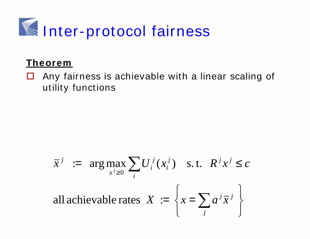
Inter-protocol fairness
Theorem� Any fairness is achievable with a linear scaling of
utility functions
==
≤=
∑
∑≥
j
jj
i
jjji
ji
x
j
xaxX
cxRxUxj
: rates achievable all
t.s. )(maxarg : 0

Inter-protocol fairness
Theorem� Any fairness is achievable with a linear scaling of
utility functions� i.e. given any x in X, there exists µ s.t. an
equilibrium p has x(p) = x
( )llll
ll
jllij
i
ji
ji
ctpyp
tpmRftpx
−=
= ∑
))((
))((1 ))((
γµ
�
Outline
� Review: homogeneous case� Motivating experiments� Model� Equilibrium
� Existence, uniqueness, local stability� Efficiency, fairness
� Slow timescale control
Tang, Wang, Low, Chiang. Infocom 2005
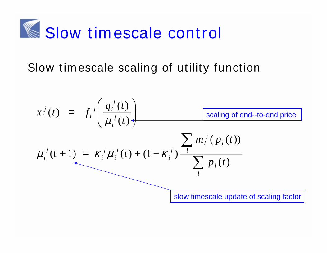
Slow timescale control
Slow timescale scaling of utility function
∑
∑−+=+
=
ll
ll
jl
ji
ji
ji
ji
ji
jij
ij
i
tp
tpmt
ttqftx
)(
))(()1()( 1)(t
)()( )(
κµκµ
µ scaling of end--to-end price
slow timescale update of scaling factor
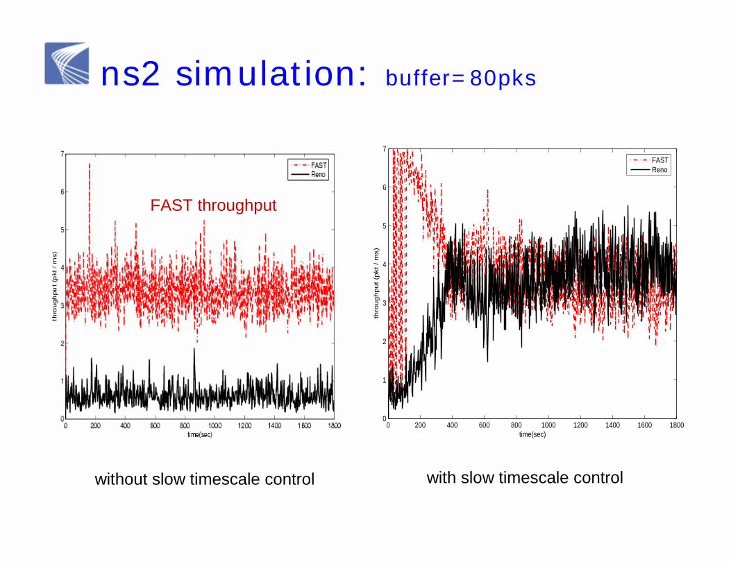
ns2 simulation: buffer=80pks
0 200 400 600 800 1000 1200 1400 1600 18000
1
2
3
4
5
6
7
time(sec)
thro
ug
hp
ut
(pkt
/ m
s)
FASTReno
FAST throughput
without slow timescale control with slow timescale control
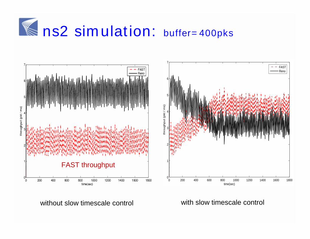
ns2 simulation: buffer=400pks
FAST throughput
without slow timescale control with slow timescale control
0 200 400 600 800 1000 1200 1400 1600 18000
1
2
3
4
5
6
7
time(sec)
thro
ug
hp
ut
(pkt
/ m
s)
FASTReno
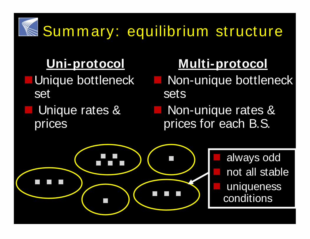
Summary: equilibrium structure
Uni-protocol�Unique bottleneck
set� Unique rates &
prices
Multi-protocol� Non-unique bottleneck
sets � Non-unique rates &
prices for each B.S.
� always odd� not all stable� uniqueness
conditions
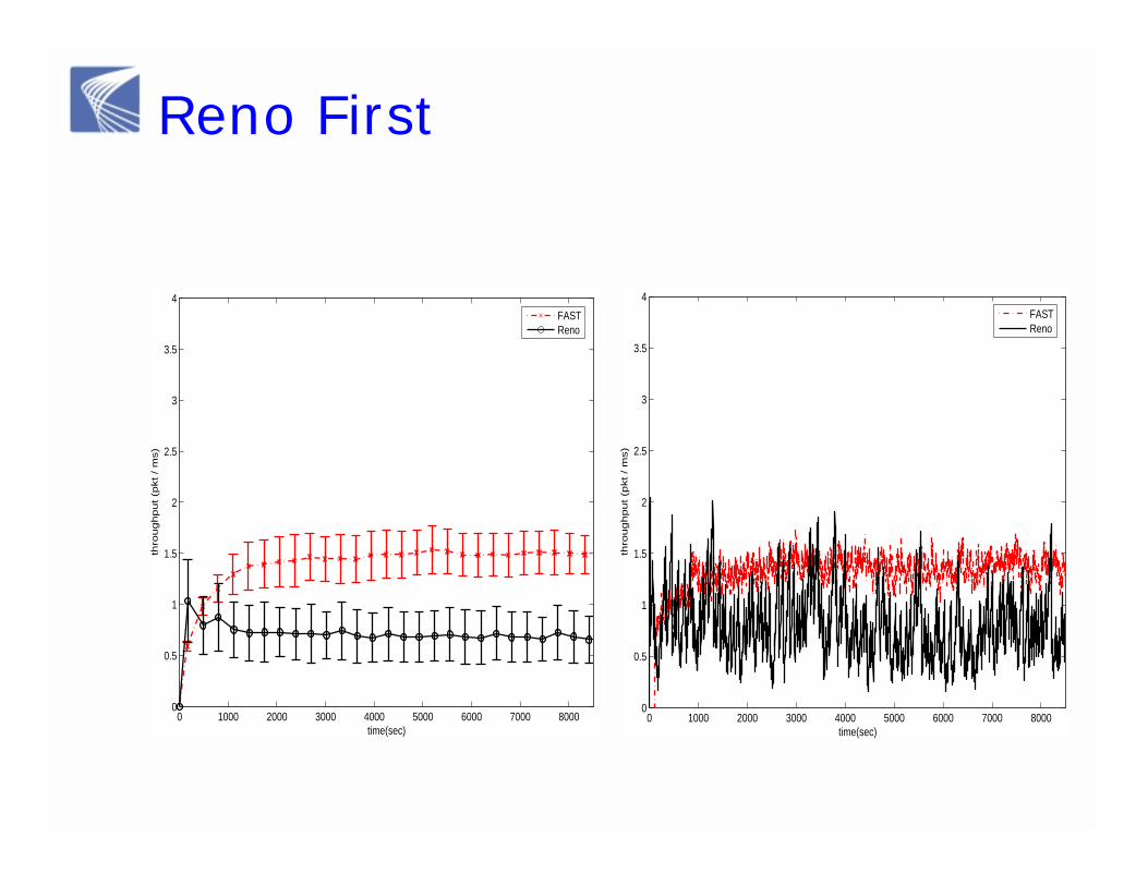
Reno First
0 1000 2000 3000 4000 5000 6000 7000 80000
0.5
1
1.5
2
2.5
3
3.5
4
time(sec)
thro
ughput (p
kt / m
s)
FASTReno
0 1000 2000 3000 4000 5000 6000 7000 80000
0.5
1
1.5
2
2.5
3
3.5
4
time(sec)
thro
ughput (p
kt / m
s)
FASTReno
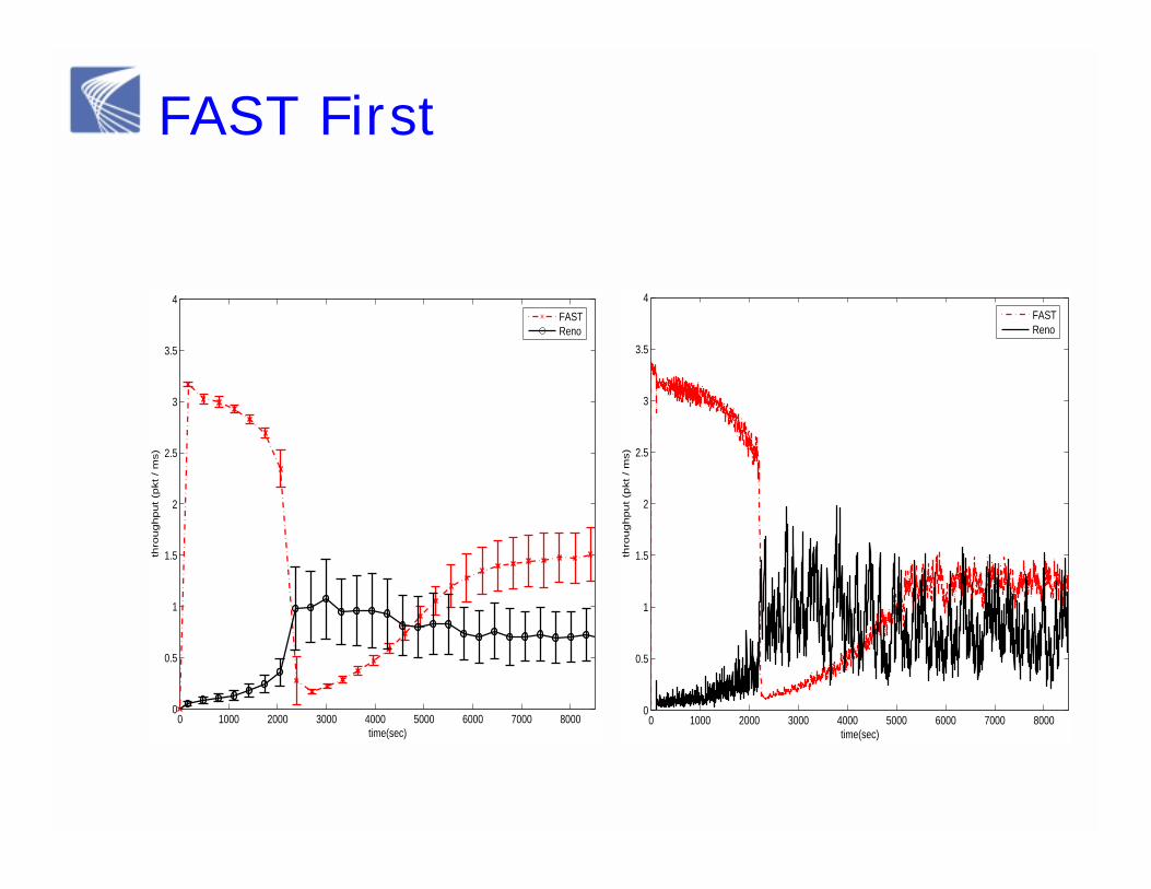
FAST First
0 1000 2000 3000 4000 5000 6000 7000 80000
0.5
1
1.5
2
2.5
3
3.5
4
time(sec)
thro
ughput (p
kt / m
s)
FASTReno
0 1000 2000 3000 4000 5000 6000 7000 80000
0.5
1
1.5
2
2.5
3
3.5
4
time(sec)
thro
ughput (p
kt / m
s)
FASTReno
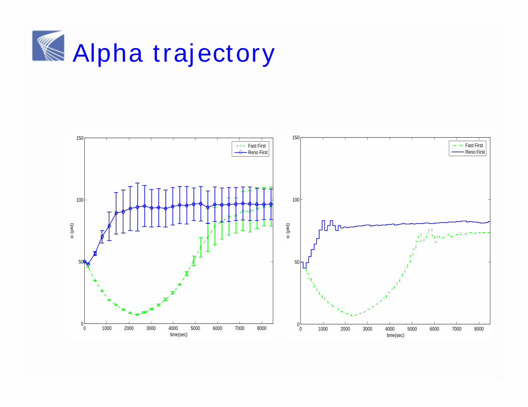
Alpha trajectory
0 1000 2000 3000 4000 5000 6000 7000 80000
50
100
150
time(sec)
α (
pkt)
Fast FirstReno First
0 1000 2000 3000 4000 5000 6000 7000 80000
50
100
150
time(sec)
α (
pkt)
Fast FirstReno First