HAL Id: tel-01668740https://hal.inria.fr/tel-01668740v2

Submitted on 6 Jan 2018

HAL is a multi-disciplinary open accessarchive for the deposit and dissemination of sci-entific research documents, whether they are pub-lished or not. The documents may come fromteaching and research institutions in France orabroad, or from public or private research centers.

L’archive ouverte pluridisciplinaire HAL, estdestinée au dépôt et à la diffusion de documentsscientifiques de niveau recherche, publiés ou non,émanant des établissements d’enseignement et derecherche français ou étrangers, des laboratoirespublics ou privés.

Heterogeneous architectures, Hybrid methods,Hierarchical matrices for Sparse Linear Solvers

Pierre Ramet

To cite this version:Pierre Ramet. Heterogeneous architectures, Hybrid methods, Hierarchical matrices for Sparse LinearSolvers. Distributed, Parallel, and Cluster Computing [cs.DC]. Université de Bordeaux, 2017. �tel-01668740v2�

UNIVERSITÉ DE BORDEAUXLABORATOIRE BORDELAIS DE RECHERCHE EN INFORMATIQUE

HABILITATION À DIRIGER DES RECHERCHES

AU TITRE DE L’ÉCOLE DOCTORALEDE MATHÉMATIQUES ET D’INFORMATIQUE

Par Pierre RAMET

Heterogeneous architectures, Hybrid methods,Hierarchical matrices for Sparse Linear Solvers

Soutenue et présentée publiquement le : 27 novembre 2017

Après avis des rapporteurs :Frédéric DESPREZ Deputy Scientific Director, InriaIain DUFF . . . . Senior Scientist, Rutherford Appleton Lab.Yousef SAAD . . . Professor, University of Minnesota

Devant la commission d’examen composée de :Iain DUFF . . . . Senior Scientist, Rutherford Appleton Lab. . . . ExaminateurRaymond NAMYST Professor, Bordeaux University . . . . . . . . . ExaminateurEsmond NG . . . . Senior Scientist, Lawrence Berkeley National Lab. ExaminateurYves ROBERT . . Professor, ENS-Lyon . . . . . . . . . . . . . . ExaminateurYousef SAAD . . . Professor, University of Minnesota . . . . . . . ExaminateurIsabelle TERRASSE Research Director, Airbus Group . . . . . . . . ExaminateurSivan TOLEDO . . Professor, Tel-Aviv University . . . . . . . . . . Examinateur

2017

2

Contents

Introduction 1

1 Static scheduling and data distributions 71.1 Context and algorithmic choices . . . . . . . . . . . . . . . . . . . . . . . . . . . . . . . . 71.2 Background . . . . . . . . . . . . . . . . . . . . . . . . . . . . . . . . . . . . . . . . . . . . 81.3 Static scheduling . . . . . . . . . . . . . . . . . . . . . . . . . . . . . . . . . . . . . . . . . 11

1.3.1 Preprocessing steps . . . . . . . . . . . . . . . . . . . . . . . . . . . . . . . . . . . . 111.3.2 Parallel scheme of the factorization . . . . . . . . . . . . . . . . . . . . . . . . . . . 111.3.3 Hybrid MPI+Thread implementation . . . . . . . . . . . . . . . . . . . . . . . . . 121.3.4 Parallel factorization algorithm . . . . . . . . . . . . . . . . . . . . . . . . . . . . . 131.3.5 Matrix mapping and task scheduling . . . . . . . . . . . . . . . . . . . . . . . . . . 15

1.4 Reducing the memory footprint using partial agregation techniques . . . . . . . . . . . . . 16

2 Dynamic scheduling and runtime systems 192.1 A dedicated approach . . . . . . . . . . . . . . . . . . . . . . . . . . . . . . . . . . . . . . 19

2.1.1 NUMA architectures . . . . . . . . . . . . . . . . . . . . . . . . . . . . . . . . . . . 192.1.2 NUMA-aware allocation . . . . . . . . . . . . . . . . . . . . . . . . . . . . . . . . . 212.1.3 Communication overlap . . . . . . . . . . . . . . . . . . . . . . . . . . . . . . . . . 222.1.4 Dynamic scheduling . . . . . . . . . . . . . . . . . . . . . . . . . . . . . . . . . . . 232.1.5 Numerical experiments . . . . . . . . . . . . . . . . . . . . . . . . . . . . . . . . . . 27

2.2 A generic approach . . . . . . . . . . . . . . . . . . . . . . . . . . . . . . . . . . . . . . . . 282.2.1 Related work . . . . . . . . . . . . . . . . . . . . . . . . . . . . . . . . . . . . . . . 292.2.2 Runtimes . . . . . . . . . . . . . . . . . . . . . . . . . . . . . . . . . . . . . . . . . 302.2.3 Supernodal factorization over DAG schedulers . . . . . . . . . . . . . . . . . . . . 332.2.4 Heterogeneous experiments . . . . . . . . . . . . . . . . . . . . . . . . . . . . . . . 39

3 Incomplete factorization and domain decomposition 433.1 Amalgamation algorithm for iLU(k) factorization . . . . . . . . . . . . . . . . . . . . . . . 43

3.1.1 Methodology . . . . . . . . . . . . . . . . . . . . . . . . . . . . . . . . . . . . . . . 443.1.2 Amalgamation algorithm . . . . . . . . . . . . . . . . . . . . . . . . . . . . . . . . 463.1.3 Numerical experiments . . . . . . . . . . . . . . . . . . . . . . . . . . . . . . . . . . 49

3.2 Graph partitioning for well balanced domain decomposition . . . . . . . . . . . . . . . . . 523.2.1 Multilevel Framework . . . . . . . . . . . . . . . . . . . . . . . . . . . . . . . . . . 553.2.2 Graph Partitioning Algorithms . . . . . . . . . . . . . . . . . . . . . . . . . . . . . 573.2.3 Experimental Results . . . . . . . . . . . . . . . . . . . . . . . . . . . . . . . . . . 63

4 Towards H-matrices in sparse direct solvers 674.1 Reordering strategy for blocking optimization . . . . . . . . . . . . . . . . . . . . . . . . . 67

4.1.1 Intra-node reordering . . . . . . . . . . . . . . . . . . . . . . . . . . . . . . . . . . 674.1.2 Related work . . . . . . . . . . . . . . . . . . . . . . . . . . . . . . . . . . . . . . . 704.1.3 Improving the blocking size . . . . . . . . . . . . . . . . . . . . . . . . . . . . . . . 70

4.2 On the use of low rank approximations in PaStiX . . . . . . . . . . . . . . . . . . . . . . 724.2.1 Block Low-Rank solver . . . . . . . . . . . . . . . . . . . . . . . . . . . . . . . . . . 734.2.2 Low-rank kernels . . . . . . . . . . . . . . . . . . . . . . . . . . . . . . . . . . . . . 754.2.3 Numerical experiments . . . . . . . . . . . . . . . . . . . . . . . . . . . . . . . . . . 78

i

4.2.4 Discussion . . . . . . . . . . . . . . . . . . . . . . . . . . . . . . . . . . . . . . . . . 83

Conclusion 87

A PaStiX 6.0 updated performance 91A.1 Experimental conditions . . . . . . . . . . . . . . . . . . . . . . . . . . . . . . . . . . . . . 91A.2 Performance on the Kepler architecture . . . . . . . . . . . . . . . . . . . . . . . . . . . . 92A.3 Performance on the KNL architecture . . . . . . . . . . . . . . . . . . . . . . . . . . . . . 92

B Bibliography 93

ii

Introduction

Over the last few decades, there have been innumerable science, engineering and societal breakthroughsenabled by the development of high performance computing (HPC) applications, algorithms and ar-chitectures. These powerful tools have provided researchers with the ability to computationally findefficient solutions for some of the most challenging scientific questions and problems in medicine andbiology, climatology, nanotechnology, energy and environment; to name a few. It is admitted todaythat numerical simulation, including data intensive treatment, is a major pillar for the development ofscientific discovery at the same level as theory and experimentation. Numerous reports and papers alsoconfirmed that extreme scale simulations will open new opportunities not only for research but also fora large spectrum of industrial and societal sectors.

An important force which has continued to drive HPC has been to focus on frontier milestones whichconsist in technical goals that symbolize the next stage of progress in the field. In the 1990s, the HPCcommunity sought to achieve computing at a teraflop rate and currently we are able to compute onthe first leading architectures at more than ten petaflops. General purpose petaflop supercomputers areavailable and exaflop computers are foreseen in early 2020.

For application codes to sustain petaflops and more in the next few years, hundreds of thousands ofprocessor cores or more are needed, regardless of processor technology. Currently, a few HPC simulationcodes easily scale to this regime and major algorithms and codes development efforts are critical toachieve the potential of these new systems. Scaling to a petaflop and more involves improving physicalmodels, mathematical modeling, super scalable algorithms.

In this context, the purpose of my research is to contribute to performing efficiently frontier simula-tions arising from challenging academic and industrial research. It involves massively parallel computingand the design of highly scalable algorithms and codes to be executed on emerging hierarchical many-core, possibly heterogeneous, platforms. Throughout this approach, I contribute to all steps that gofrom the design of new high-performance more scalable, robust and more accurate numerical schemesto the optimized implementations of the associated algorithms and codes on very high performancesupercomputers. This research is conducted in close collaboration with European and US initiatives.

Thanks to three associated teams, namely PhyLeaS 1, MORSE 2 and FASTLA 3, I have contributedwith world leading groups to the design of fast numerical solvers and their parallel implementation.

I For the solution of large sparse linear systems, we design numerical schemes and software packagesfor direct and hybrid parallel solvers. Sparse direct solvers are mandatory when the linear system isvery ill-conditioned; such a situation is often encountered in structural mechanics codes, for example.Therefore, to obtain an industrial software tool that must be robust and versatile, high-performancesparse direct solvers are mandatory, and parallelism is then necessary for reasons of memory capabilityand acceptable solution time. Moreover, in order to solve efficiently 3D problems with more than 50million unknowns, which is now a reachable challenge with new multicore supercomputers, we mustachieve good scalability in time and control memory overhead. Solving a sparse linear system by a directmethod is generally a highly irregular problem that provides some challenging algorithmic problemsand requires a sophisticated implementation scheme in order to fully exploit the capabilities of modernsupercomputers. It would be hard work to provide here a complete survey on direct methods for sparselinear systems and the corresponding software. Jack Dongarra has maintained for many years a list of

1http://www-sop.inria.fr/nachos/phyleas/2http://icl.cs.utk.edu/morse/3https://www.inria.fr/en/associate-team/fastla

1

freely available software packages for linear algebra 4. And a recent survey by Tim Davis et al. has beenpublished [44] with a list of available software in the last section.

New supercomputers incorporate many microprocessors which are composed of one or many compu-tational cores. These new architectures induce strongly hierarchical topologies. These are called NUMAarchitectures. In the context of distributed NUMA architectures, we study optimization strategies to im-prove the scheduling of communications, threads and I/O. In the 2000s, our first attempts to use availablegeneric runtime systems, such as PM2 [15] or Athapascan [25], failed to reach acceptable performance.We then developed dedicated dynamic scheduling algorithms designed for NUMA architectures in thePaStiX solver. The data structures of the solver, as well as the patterns of communication have beenmodified to meet the needs of these architectures and dynamic scheduling. We are also interested inthe dynamic adaptation of the computational granularity to use efficiently multi-core architectures andshared memory. Several numerical test cases have been used to prove the efficiency of the approach ondifferent architectures.

The pressure to maintain reasonable levels of performance and portability forces application develop-ers to leave the traditional programming paradigms and explore alternative solutions. We have studiedthe benefits and limits of replacing the highly specialized internal scheduler of the PaStiX solver withgeneric runtime systems. The task graph of the factorization step is made available to the runtimessystems, allowing them to process and optimize its traversal in order to maximize the algorithm effi-ciency for the targeted hardware platform. The aim was to design algorithms and parallel programmingmodels for implementing direct methods for the solution of sparse linear systems on emerging computersequipped with GPU accelerators. More generally, this work was performed in the context of the asso-ciated team MORSE and the ANR SOLHAR project which aims at designing high performance sparsedirect solvers for modern heterogeneous systems. The main competitors in this research area are theQR-MUMPS and SuiteSparse packages, mainly the CHOLMOD (for sparse Cholesky factorizations)and SPQR (for sparse QR factorizations) solvers that achieve a rather good speedup using several GPUaccelerators but only using one node (shared memory). In collaboration with the ICL team from theUniversity of Tennessee, a comparative study of the performance of the PaStiX solver on top of itsnative internal scheduler, PaRSEC, and StarPU frameworks, on different execution environments, hasbeen performed. The analysis highlights that these generic task-based runtimes achieve comparable re-sults to the application-optimized embedded scheduler on homogeneous platforms. Furthermore, theyare able to significantly speed up the solver on heterogeneous environments by taking advantage of theaccelerators while hiding the complexity of their efficient manipulation from the programmer.

More recently, many works have addressed heterogeneous architectures to exploit accelerators suchas GPUs or Intel Xeon Phi with interesting speedup. Despite research towards generic solutions toefficiently exploit those accelerators, their hardware evolution requires continual adaptation of the kernelsrunning on those architectures. The recent Nvidia architectures, such as Kepler, present a larger numberof parallel units thus requiring more data to feed every computational unit. A solution considered forsupplying enough computation has been studied on problems with a large number of small computations.The batched BLAS libraries proposed by Intel, Nvidia, or the University of Tennessee are examples of thissolution. We have investigated the use of the variable size batched matrix-matrix multiply to improvethe performance of the PaStiX sparse direct solver. Indeed, this kernel suits the supernodal method ofthe solver, and the multiple updates of variable sizes that occur during the numerical factorization.

I In addition to the main activities on direct solvers, we also studied some robust preconditioningalgorithms for iterative methods. The goal of these studies is to overcome the huge memory consumptioninherent to the direct solvers in order to solve 3D problems of huge size. Our study was focused onthe building of generic parallel preconditioners based on incomplete LU factorizations. The classicalincomplete LU preconditioners use scalar algorithms that do not exploit well CPU power and are difficultto parallelize. Our work was aimed at finding some new orderings and partitionings that lead to a denseblock structure of the incomplete factors. Then, based on the block pattern, some efficient parallelblockwise algorithms can be devised to build robust preconditioners that are also able to fully exploitthe capabilities of modern high-performance computers.

The first approach was to define an adaptive blockwise incomplete factorization that is much moreaccurate (and numerically more robust) than the scalar incomplete factorizations commonly used to pre-condition iterative solvers. Such incomplete factorization can take advantage of the latest breakthroughs

4http://www.netlib.org/utk/people/JackDongarra/la-sw.html

2

in sparse direct methods and particularly should be very competitive in CPU time (effective power usedfrom processors and good scalability) while avoiding the memory limitation encountered by direct meth-ods. In this way, we expected to be able to solve systems in the order of a hundred million unknownsand even one billion unknowns. Another goal was to analyze and justify the chosen parameters that canbe used to define the block sparse pattern in our incomplete factorization. The driving rationale for thisstudy is that it is easier to incorporate incomplete factorization methods into direct solution softwarethan it is to develop new incomplete factorizations. Our main goal at this point was to achieve a sig-nificant reduction in the memory needed to store the incomplete factors (with respect to the completefactors) while keeping enough fill-in to make the use of BLAS3 (in the factorization) and BLAS2 (in thetriangular solves) primitives profitable. In this approach, we focused on the critical problem of findingapproximate supernodes of ILU(k) factorizations. The problem was to find a coarser block structure ofthe incomplete factors. The “exact” supernodes that are exhibited from the incomplete factor nonzeropattern are usually very small and thus the resulting dense blocks are not large enough for efficient useof the BLAS3 routines. A remedy to this problem was to merge supernodes that have nearly the samestructure. These algorithms have been implemented in the PaStiX library.

A second approach is the use of hybrid methods that hierarchically combine direct and iterativemethods. These techniques inherit the advantages of each approach, namely the limited amount ofmemory and natural parallelization for the iterative component and the numerical robustness of thedirect part. The general underlying ideas are not new since they have been intensively used to designdomain decomposition techniques; these approaches cover a fairly large range of computing techniquesfor the numerical solution of partial differential equations (PDEs) in time and space. Generally speaking,it refers to the splitting of the computational domain into subdomains with or without overlap. Thesplitting strategy is generally governed by various constraints/objectives but the main one is to expressparallelism. The numerical properties of the PDEs to be solved are usually intensively exploited at thecontinuous or discrete levels to design the numerical algorithms so that the resulting specialized techniquewill only work for the class of linear systems associated with the targeted PDE. Under this framework,Pascal Hénon and Jérémie Gaidamour [50] have developed in collaboration with Yousef Saad, fromUniversity of Minnesota, algorithms that generalize the notion of “faces” and “edges” of the “wire-basket”decomposition. The interface decomposition algorithm is based on defining a “hierarchical interfacestructure” (HID). This decomposition consists in partitioning the set of unknowns of the interface intocomponents called connectors that are grouped in “classes” of independent connectors [78]. This has ledto software developments on the design of algebraic non-overlapping domain decomposition techniquesthat rely on the solution of a Schur complement system defined on the interface introduced by thepartitioning of the adjacency graph of the sparse matrix associated with the linear system. Differenthierarchical preconditioners can be considered, possibly multilevel, to improve the numerical behavior ofthe approaches implemented in HIPS [51] and MaPHYS [2]. For both software libraries the principleis to build a decomposition of the adjacency matrix of the system into a set of small subdomains.This decomposition is built from the nested dissection separator tree obtained using the sparse matrixreordering software Scotch. Thus, at a certain level of the separator tree, the subtrees are consideredas the interior of the subdomains and the union of the separators in the upper part of the eliminationtree constitutes the interface between the subdomains. The interior of these subdomains are treated by adirect method, such as PaStiX or MUMPS. Solving the whole system is then equivalent to solving theSchur complement system on the interface between the subdomains which has a much smaller dimension.The PDSLIN package is another parallel software for algebraic methods based on Schur complementtechniques that is developed at Lawrence Berkeley National Laboratory. Other related approaches basedon overlapping domain decomposition (Schwarz type) ideas are more widely developed and implementedin software packages at Argonne National Laboratory (software contribution to PETSc where RestrictiveAdditive Schwarz is the default preconditioner) and at Sandia National Laboratories (ShyLU in theTrilinos package).

I Nested dissection is a well-known heuristic for sparse matrix ordering to both reduce the fill-in duringnumerical factorization and to maximize the number of independent computational tasks. By using theblock data structure induced by the partition of separators of the original graph, very efficient parallelblock solvers have been designed and implemented according to supernodal or multifrontal approaches.Considering hybrid methods mixing both direct and iterative solvers such as HIPS or MaPHYS, ob-taining a domain decomposition leading to a good balancing of both the size of domain interiors and the

3

size of interfaces is a key point for load balancing and efficiency in a parallel context. We have revisitedsome well-known graph partitioning techniques in the light of the hybrid solvers and have designed newalgorithms to be tested in the Scotch package. These algorithms have been integrated in Scotch as aprototype.

On the other hand, the preprocessing steps of sparse direct solvers, ordering and block-symbolicfactorization, are two major steps that lead to a reduced amount of computation and memory and toa better task granularity to reach a good level of performance when using BLAS kernels. With theadvent of GPUs, the granularity of the block computations became more important than ever. In thiswork, we present a reordering strategy that increases this block granularity. This strategy relies on theblock-symbolic factorization to refine the ordering produced by tools such as MeTiS or Scotch, but ithas no impact on the number of operations required to solve the problem. We integrate this algorithmin the PaStiX solver and show an important reduction in the number of off-diagonal blocks on a largespectrum of matrices. Furthermore, we propose a parallel implementation of our reordering strategy,leading to a computational cost that is really low with respect to the numerical factorization and that iscounterbalanced by the improvement to the factorization time. In addition, if multiple factorizations areapplied on the same structure, this benefits the additional factorization and solve steps at no extra cost.We proved that such a preprocessing stage is cheap in the context of 3D graphs of bounded degree, andshowed that it works well for a large set of matrices. We compared this with the HSL reordering [134, 80],which targets the same objective of reducing the overall number of off-diagonal blocks. While our TSP(Travelling Salesman Problem) heuristic is often more expensive, the quality is always improved, leadingto better performance. In the context of multiple factorizations, or when using GPUs, the TSP overheadis recovered by performance improvement, while it may be better to use HSL for the other cases.

I The use of low-rank approximations in sparse direct methods is ongoing work. When applying Gaussianelimination, the Schur complement induced appears to exhibit this low-rank property in several physicalapplications, especially those arising from elliptic partial differential equations. This property on thelow rank of submatrices may then be exploited. Each supernode or front may then be expressed in alow-rank approximation representation. Finally, solvers that exploit this low-rank property may be usedeither as accurate direct solvers or as powerful preconditioners for iterative methods, depending on howmuch information is kept.

In the context of the FASTLA associated team, in collaboration with E. Darve from Stanford Uni-versity, we have been working on applying fast direct solvers for dense matrices to the solution of sparsedirect systems with a supernodal approach. We observed that the extend-add operation (during thesparse factorization) is the most time-consuming step. We have therefore developed a series of algo-rithms to reduce this computational cost. We have presented two approaches using a Block Low-Rank(BLR) compression technique to reduce the memory footprint and/or the time-to-solution of the sparsesupernodal solver PaStiX. This flat, non-hierarchical, compression method allows us to take advantageof the low-rank property of the blocks appearing during the factorization of sparse linear systems, whichcome from the discretization of partial differential equations. The first approach, called Minimal Mem-ory, illustrates the maximum memory gain that can be obtained with the BLR compression method,while the second approach, called Just-In-Time, mainly focuses on reducing the computational complex-ity and thus the time-to-solution. We compare Singular Value Decomposition (SVD) and Rank-RevealingQR (RRQR), as compression kernels, in terms of factorization time, memory consumption, as well asnumerical properties.

To improve the efficiency of our sparse update kernel for both BLR (block low-rank) and HODLR(hierarchically off-diagonal low-rank), we are now investigating a BDLR (boundary distance low-rank)approximation scheme to preselect rows and columns in the low-rank approximation algorithm. We alsohave to improve our ordering strategies to enhance data locality and compressibility. The implementationis based on runtime systems to exploit parallelism.

Regarding our activities around the use of hierarchical matrices for sparse direct solvers, this topicis also widely investigated by our competitors. Some related work is described in the last section of thisreport, but we mention here the following codes :

• STRUMPACK uses Hierarchically Semi-Separable (HSS) matrices for low-rank structured factor-ization with randomized sampling.

• MUMPS uses Block Low-Rank (BLR) approximations to improve a multifrontal sparse solver.

4

I This report mainly concerns my work on the PaStiX sparse linear solvers, developed thanks to along-term collaboration with CEA/CESTA. But I also contributed to external applications through jointresearch efforts with academic partners enabling efficient and effective technological transfer towardsindustrial R&D. Outside the scope of this document, I would like to summarize here some of thesecontributions.

• Plasma physic simulation: scientific simulation for ITER tokamak modeling provides a naturalbridge between theory and experiment and is also an essential tool for understanding and predictingplasma behavior. Recent progress in numerical simulation of fine-scale turbulence and in large-scaledynamics of magnetically confined plasma has been enabled by access to petascale supercomputers.This progress would have been unreachable without new computational methods and adaptedreduced models. In particular, the plasma science community has developed codes for whichcomputer runtime scales quite well with the number of processors up to thousands cores. Othernumerical simulation tools designed for the ITER challenge aim at making significant progressin understanding active control methods of plasma edge MHD instability Edge Localized Modes(ELMs) which represent a particular danger with respect to heat and particle loads for PlasmaFacing Components (PFC) in the tokamak. The goal is to improve the understanding of therelated physics and to propose possible new strategies to improve effectiveness of ELM controltechniques. The simulation tool used (JOREK code) is related to non linear MHD modeling andis based on a fully implicit time evolution scheme that leads to 3D large very badly conditionedsparse linear systems to be solved at every time step. In this context, the use of the PaStiX libraryto solve efficiently these large sparse problems by a direct method was a challenging issue [81].Please look at http://www.labri.fr/perso/ramet/restricted/HDR_PPCF09.pdf for a full ver-sion of this work with some experiments made during the PhD thesis of Xavier Lacoste [95].

• Nuclear core simulation: EDF R&D is developing a nuclear core simulation code namedCOCAGNE that relies on a Simplified PN (SPN) method for eigenvalue calculations to computethe neutron flux inside the core. In order to assess the accuracy of SPN results, a 3D Cartesianmodel of PWR nuclear cores has been designed and a reference neutron flux inside this core hasbeen computed with a Monte Carlo transport code from Oak Ridge National Lab. This kind of3D whole core probabilistic evaluation of the flux is computationally very expensive. An efficientdeterministic approach is therefore required to reduce the computation cost dedicated to referencesimulations. First, we have completed a study to parallelize an SPN simulation code by using adomain decomposition method, applied for the solution of the neutron transport equations (Boltz-mann equations), based on the Schur dual technique and implemented in the COCAGNE code fromEDF. This approach was very reliable and efficient on computations coming from the IAEA bench-mark and from industrial cases [22]. Secondly, we worked on the parallelization of the DOMINOcode, a parallel 3D Cartesian SN solver specialized for PWR core reactivity computations. Wehave developed a two-level (multi-core + SIMD) parallel implementation of the sweep algorithmon top of runtime systems [112].Please look at http://www.labri.fr/perso/ramet/restricted/HDR_JCP10.pdf and also at http://www.labri.fr/perso/ramet/restricted/HDR_JCP17.pdf (submitted to JCP) for a full versionof this work with some experiments made during the PhD thesis of Bruno Lathuiliere [97] and SalliMoustafa [111].

• Electromagnetism simulation: in collaboration with CEA/CESTA, during his PhD thesis [35],Mathieu Chanaud developed a new parallel platform based on a combination of a multigrid solverand a direct solver (PaStiX) to solve huge linear systems arising from Maxwell’s equations dis-cretized with first-order Nédelec elements [36]. In the context of the HPC-PME initiative, wealso started a collaboration with AlgoTech and we have organized one of the first PhD-consultantactions at Inria implemented by Xavier Lacoste and led by myself. AlgoTech is one of the mostinnovative SMEs (small and medium-sized enterprises) in the field of cabling embedded systems,and more broadly, automatic devices. The main target of the project was to validate our sparselinear solvers in the area of electromagnetic simulation tools developed by AlgoTech.

5

I This report is organized as follows. In Chapter 1, we recall the original implementation of the PaStiXsolver based on static scheduling that was well suited for homogeneous architectures. Thanks to theexpertise of Pascal Hénon, we developed our basic kernels for the analysis steps that are still relevantfor our prediction models. Chapter 2 presents the two approaches we have investigated to address theneed for dynamic scheduling when architectures becomes too difficult to model. The second approachis probably the most promising because it allows us to deal with GPU accelerators and Intel Xeon Phiwhile obtaining rather good efficiency and scalability. In Chapter 3, we first recall our contribution onparallel implementation of an ILU(k) algorithm within the PaStiX framework. This solution allowsus to reduce the memory needed by the numerical factorization. Compared to the other incompletefactorization methods and hybrid solvers based on domain decomposition, we do not need to considernumerical information from the linear system. But the gain in terms of flops and memory is not enoughin many cases to compete with multigrid solvers for instance. The second part of this chapter describessome preliminary work regarding using graph partitioning techniques to build a domain decompositionleading to a good balancing of both the interface and the internal nodes of each subdomain, which is arelevant criteria to optimize parallel implementation of hybrid solvers. Finally, we introduce a reorderingstrategy to improve the blocking arising during the symbolic factorization in Chapter 4. Our attempt toapply fast direct solvers for dense matrices to the solution of sparse direct systems is presented in thesecond part of this chapter and benefits from both our graph partitioning and reordering heuristics.

6

Chapter 1

Static scheduling and datadistributions

This chapter presents some unpublished technical elements that have been introduced in the PaStiXsolver to enable MPI+Threads paradigm. This joint work with Pascal Hénon extends the contributionsthat have been published in [74, 75].

Please look at http://www.labri.fr/perso/ramet/restricted/HDR_PC02.pdf for a full version ofthis work with some experiments.

1.1 Context and algorithmic choicesSolving large sparse symmetric positive definite systems Ax = b of linear equations is a crucial and time-consuming step, arising in many scientific and engineering applications. For a complete survey on directmethods, one can refer to [46, 53, 54]. Due to their robustness, direct solvers are often used in industrialcodes despite their memory consumption. In addition, the factorization today’s used in direct solversare able to take advantage of the superscalar capabilities of the processors by using blockwise algorithmsand BLAS primitives. Consequently, many parallel techniques for sparse matrix factorization have beenstudied and implemented. The goal of our work was to design efficient algorithms that were able to takeadvantage of the architectures of the modern parallel computers. In our work, we did not consider thefactorization with dynamic pivoting and we only considered matrices with a symmetric sparsity pattern(A + At can be used for unsymmetric cases). In this context, the block structure of the factors andthe numerical operations are known in advance and consequently allow the use of static (i.e. beforethe effective numerical factorization) regulation algorithms for the distribution and the computationaltask scheduling. Therefore, we developed some high performing algorithms for the direct factorizationthat were able to exploit very strongly the specificities of the networks and processors of the targetedarchitectures. In this work, we present some static assignments heuristics and an associated factorizationalgorithm that achieve very performant results for both runtime and memory overhead reduction.

There are two main approaches for numerical factorization algorithms: the multifrontal approach [6,47], and the supernodal one [67, 127].

Both can be described by a computational tree whose nodes represent computations and whose edgesrepresent transfer of data. In the case of the multifrontal method, at each node, some steps of Gaussianelimination are performed on a dense frontal matrix and the remaining Schur complement, or contributionblock, is passed to the parent node for assembly. In the case of the supernodal method, the distributedmemory version uses a right-looking formulation which, having computed the factorization of a column-block corresponding to a node of the tree, then immediately sends the data to update the column-blockscorresponding to ancestors in the tree. In a parallel context, we can locally aggregate contributions tothe same block before sending the contributions. This can significantly reduce the number of messages.

Independently of these different methods, a static or dynamic scheduling of block computations canbe used. For homogeneous parallel architectures, it is useful to find an efficient static scheduling [121].In this context, this scheduling can be induced by a fine cost computation/communication model.

7

The PSPASES solver [85] is based on a multifrontal approach without pivoting for symmetric pos-itive definite systems. It uses MeTiS [87] for computing a fill-reducing ordering which is based on amultilevel nested dissection algorithm; when the graph is separated into p parts, a multiple minimumdegree (MMD [102]) is then used. A “subtree to subcube”-like algorithm is applied to build a staticmapping before the numerical factorization. In [7] the performance of MUMPS [4] and SuperLU [99]are compared for nonsymmetric problems. MUMPS uses a multifrontal approach with dynamic pivotingfor stability while SuperLU is based on a supernodal technique with static pivoting.

In previous work [74, 75], we have proposed some high performing algorithms for high performancesparse supernodal factorization without pivoting. These techniques yield a static mapping and schedul-ing algorithm based on a combination of 1D and 2D block distributions. Thus, we achieved very goodperformance by taking into account all the constraints of the problem as well as the specificities (commu-nication and computation) of the parallel architecture. In addition, we have studied a way to control thememory overhead due to the buffering needed to reduce the communication volume. In the case of oursupernodal factorization, this buffering corresponds to the local aggregation approach in which all localcontributions for the same non-local block are summed in a temporary block buffer before being sent(see section 1.3). Consequently, we have improved the mechanism of local aggregation that may leadto great overheads of memory consumption for 3D problems in an all-distributed memory context. In[76] we presented the mechanism to control this memory overhead that preserves relatively good runtimeperformance.

We have implemented our algorithms in a library called PaStiX that manages L.Lt, L.D.Lt factor-izations and more generally L.U factorization when the symmetrized pattern A+ At is considered. Wehave both real and complex version for the L.D.Lt and L.U factorization. The PaStiX library has beensuccessfully used in industrial simulation codes to solve systems of several million unknowns [59, 60].Until now, our study was suitable for homogeneous parallel/distributed architectures in the context of amessage passing paradigm.

In the context of Symmetric Multi-Processing (SMP) node architectures, to fully exploit sharedmemory advantages, a relevant approach is to use a hybrid MPI+Thread implementation. This approachin the framework of direct solvers aims to solve problems with more than 10 million unknowns, whichis now a reachable challenge with new SMP supercomputers. The rational that motivated this hybridimplementation was that the communications within an SMP node can be advantageously substitutedby direct accesses to shared memory between the processors in the SMP node using threads. In addition,the MPI-communication between processes are grouped by SMP nodes. Consequently, whereas in thepure MPI implementation the static mapping and scheduling were computed by MPI process, in the newMPI+Thread implementation, the mapping is still computed by MPI process but the task scheduling iscomputed by thread.

1.2 BackgroundThis section provides a brief background on sparse Gaussian elimination techniques, including their graphmodels. Details can be found in [40, 46, 54] among others. Consider the linear system

Ax = b (1.1)

where A is a symmetric definite positive matrix of size n×n or a unsymmetric matrix with a symmetricnonzero pattern. In this contex, sparse matrix techniques often utilize the non-oriented adjacency graphG = (V,E) of the matrix A, a graph whose n vertices represent the n unknowns, and whose edges(i, j) represent the couplings between unknowns i and j. The Gaussian Elimination (L.Lt Choleskyfactorization or L.U factorization) process introduces “fill-in”s, i.e., new edges in the graph. The qualityof the direct solver depends critically on the ordering of the unknowns as this has a major impact on thenumber of fill-ins generated.

Sparse direct solvers often utilize what is known as the “filled graph” of A, which is the graph of the(complete) Cholesky factor L, or rather of L + U . This is the original graph augmented with all thefill-in generated during the elimination process. We will denote by G∗ = (V,E∗) this graph.

Two well-known and useful concepts will be needed in later sections. The first is that of fill paths. Thisis a path between two nodes i and j (with i 6= j) in the original graph G = (V,E), whose intermediate

8

nodes are all numbered lower than both i and j. A theorem by Rose and Tarjan [100] states that thereis a fill path between i and j if and only if (i, j) is in E∗, i.e., there will be a fill-in in position (i, j).

The second important concept is that of an elimination tree [103], which is useful among other things,for scheduling the tasks of the solver in a parallel environment [8, 75]. The elimination tree captures thedependency between columns in the factorization. It is defined from the filled graph using the parentrelationship:

parent(j) = min{i |i > j and (i, j) ∈ E∗} .Two broad classes of reorderings for sparse Gaussian elimination have been widely utilized. The

first, which tends to be excellent at reducing fill-in is the minimal degree ordering. This method, whichhas many variants, is a local heuristic based on a greedy algorithm [5]. The class of nested dissectionalgorithms [54], considered in this work, is common in the “static” variants of Gaussian elimination whichpreorder the matrix and define the tasks to be executed in parallel at the outset. The nested dissectionordering utilizes recursively a sequence of separators. A separator C is a set of nodes which splits thegraph into two subgraphs G1 and G2 such that there is no edge linking a vertex of G1 to a vertex of G2.This is then done recursively on the subgraphs G1 and G2. The left side of Figure 1.1 shows an exampleof a physical domain (e.g., a finite element mesh) partitioned recursively in this manner into a total of8 subgraphs. The labeling used by Nested Dissection can be defined recursively as follows: label thenodes of the separator last after (recursively) labeling the nodes of the children. This defines naturallya tree structure as shown in the right side of Figure 1.1. The remaining subgraphs are then ordered bya minimum degree algorithm under constraints [117].

C

C

C

C

C7

3

4

1

26

C

C5

C

C

CCC

C

C

7

6 3

5 4 2 1

D D D D D DDD8 5 4 3 2 17 6

Figure 1.1: The nested dissection of a physical mesh and corresponding tree

An ideal separator is such that G1 and G2 are of about the same size while the set C is small. Anumber of efficient graph partitioners have been developed in recent years which attempt to reach acompromise between these two requirements, see, e.g., [87, 116, 71] among others.

After a good ordering is found a typical solver peforms a symbolic factorization which essentiallydetermines the pattern of the factors. This phase can be elegantly expressed in terms of the eliminationtree. We will denote by [i] the sparse pattern of a column i which is the list of rows indices in increasingorder corresponding to nonzeros terms.

Algorithm 1: Sequential symbolic factorization algorithmBuild [i] for each column i in the original graph;for i = 1 . . . n− 1 do

[parent(i)] = merge ([i], [parent(i)]) ;

where merge([i],[j]) is a function which merges the patterns of column i and j in the lower triangularfactor. In a parallel implementation, this is better done with the help of a post-order traversal of thetree: the pattern of a given node only depends on the patterns of the children and can be obtained oncethese are computed. The symbolic factorization is a fairly inexpensive process since it utilizes two nestedloops instead of the three loops normally required by Gaussian elimination. Note that all computationsare symbolic, the main kernel being the merge of two column patterns.

Most sparse direct solvers take advantage of dense computations by exhibiting a dense block structurein the matrix L. This dense block structure is directly linked to the ordering techniques based on the

9

nested dissection algorithm (ex: MeTiS [87] or Scotch [118]). Indeed the columns of L can be groupedin sets such that all columns of a same set have a similar non zero pattern. Those sets of columns,called supernodes, are then used to prune the block structure of L. The supernodes obtained with suchorderings mostly correspond to the separators found in the nested dissection process of the adjacencygraph G of matrix A.

An important result used in direct factorization is that the partition P of the unknowns induced bythe supernodes can be found without knowing the non zero pattern of L [104]. The partition P of theunknowns is then used to compute the block structure of the factorized matrix L during the so-calledblock symbolic factorization. The block symbolic factorization exploits the fact that, when P is thepartition of separators obtained by nested dissection then we have:

Q(G,P)∗ = Q(G∗,P)

where Q(G,P) is the quotient graph of G with regards to partition P. Then, we can deduce the blockelimination tree which is the elimination tree associated with Q(G,P)∗ and which is well suited forparallelism [75]. It is important to keep in mind that this property can be used to prune the blockstructure of the factor L because one can find the supernode partition from G(A) [104].

1

2

3

4

5

6

7

8

9

10

11

12

13

14

15

16

17

18

19

20

21

22

23

24

25

26

27

28

29

30

31

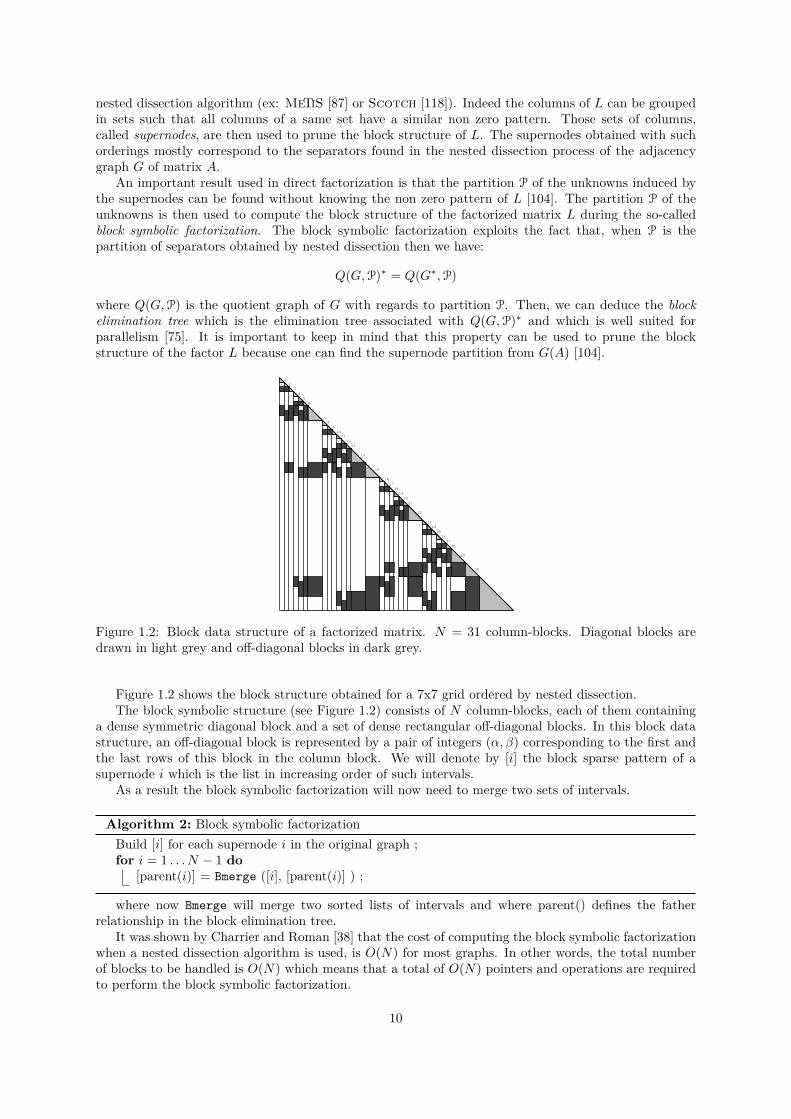
Figure 1.2: Block data structure of a factorized matrix. N = 31 column-blocks. Diagonal blocks aredrawn in light grey and off-diagonal blocks in dark grey.

Figure 1.2 shows the block structure obtained for a 7x7 grid ordered by nested dissection.The block symbolic structure (see Figure 1.2) consists of N column-blocks, each of them containing

a dense symmetric diagonal block and a set of dense rectangular off-diagonal blocks. In this block datastructure, an off-diagonal block is represented by a pair of integers (α, β) corresponding to the first andthe last rows of this block in the column block. We will denote by [i] the block sparse pattern of asupernode i which is the list in increasing order of such intervals.

As a result the block symbolic factorization will now need to merge two sets of intervals.

Algorithm 2: Block symbolic factorizationBuild [i] for each supernode i in the original graph ;for i = 1 . . . N − 1 do

[parent(i)] = Bmerge ([i], [parent(i)] ) ;

where now Bmerge will merge two sorted lists of intervals and where parent() defines the fatherrelationship in the block elimination tree.

It was shown by Charrier and Roman [38] that the cost of computing the block symbolic factorizationwhen a nested dissection algorithm is used, is O(N) for most graphs. In other words, the total numberof blocks to be handled is O(N) which means that a total of O(N) pointers and operations are requiredto perform the block symbolic factorization.

10

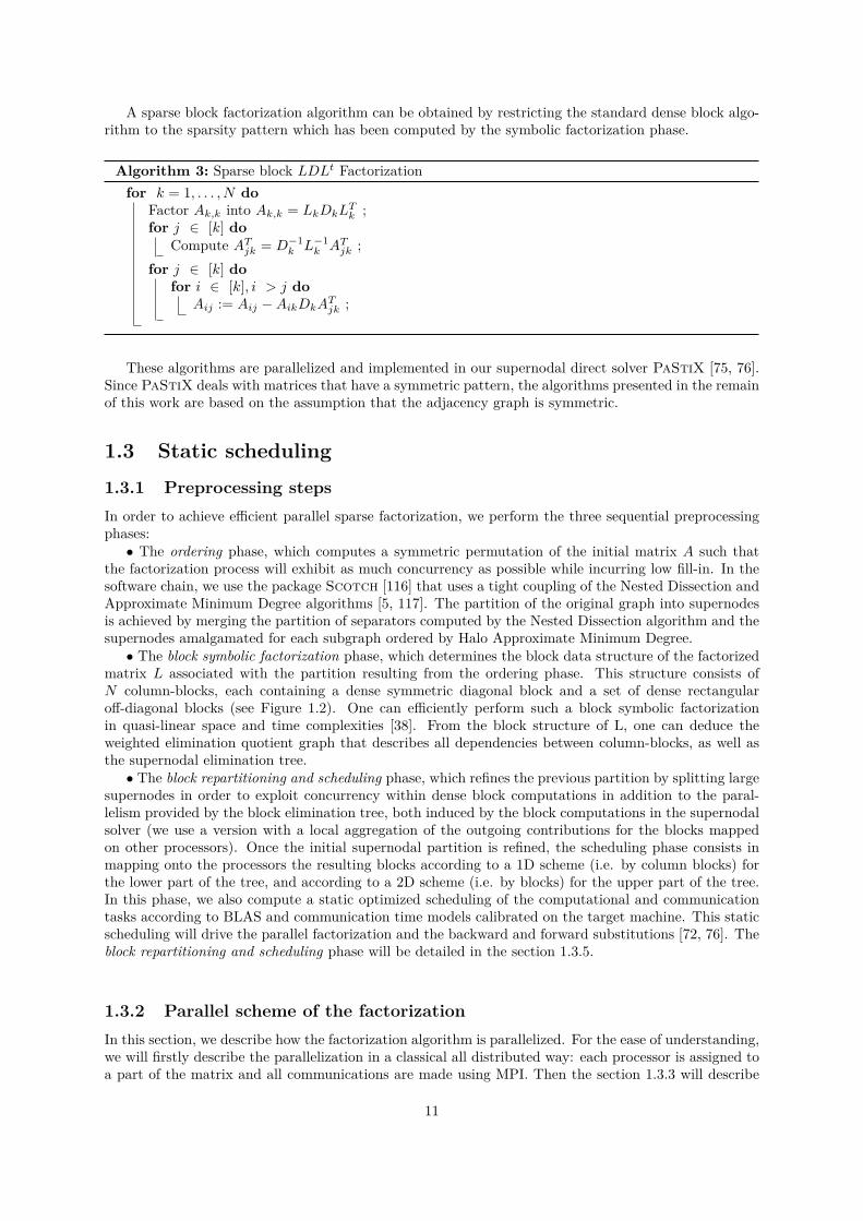
A sparse block factorization algorithm can be obtained by restricting the standard dense block algo-rithm to the sparsity pattern which has been computed by the symbolic factorization phase.

Algorithm 3: Sparse block LDLt Factorizationfor k = 1, . . . , N do

Factor Ak,k into Ak,k = LkDkLTk ;

for j ∈ [k] doCompute ATjk = D−1

k L−1k ATjk ;

for j ∈ [k] dofor i ∈ [k], i > j do

Aij := Aij −AikDkATjk ;

These algorithms are parallelized and implemented in our supernodal direct solver PaStiX [75, 76].Since PaStiX deals with matrices that have a symmetric pattern, the algorithms presented in the remainof this work are based on the assumption that the adjacency graph is symmetric.

1.3 Static scheduling1.3.1 Preprocessing stepsIn order to achieve efficient parallel sparse factorization, we perform the three sequential preprocessingphases:• The ordering phase, which computes a symmetric permutation of the initial matrix A such that

the factorization process will exhibit as much concurrency as possible while incurring low fill-in. In thesoftware chain, we use the package Scotch [116] that uses a tight coupling of the Nested Dissection andApproximate Minimum Degree algorithms [5, 117]. The partition of the original graph into supernodesis achieved by merging the partition of separators computed by the Nested Dissection algorithm and thesupernodes amalgamated for each subgraph ordered by Halo Approximate Minimum Degree.• The block symbolic factorization phase, which determines the block data structure of the factorized

matrix L associated with the partition resulting from the ordering phase. This structure consists ofN column-blocks, each containing a dense symmetric diagonal block and a set of dense rectangularoff-diagonal blocks (see Figure 1.2). One can efficiently perform such a block symbolic factorizationin quasi-linear space and time complexities [38]. From the block structure of L, one can deduce theweighted elimination quotient graph that describes all dependencies between column-blocks, as well asthe supernodal elimination tree.• The block repartitioning and scheduling phase, which refines the previous partition by splitting large

supernodes in order to exploit concurrency within dense block computations in addition to the paral-lelism provided by the block elimination tree, both induced by the block computations in the supernodalsolver (we use a version with a local aggregation of the outgoing contributions for the blocks mappedon other processors). Once the initial supernodal partition is refined, the scheduling phase consists inmapping onto the processors the resulting blocks according to a 1D scheme (i.e. by column blocks) forthe lower part of the tree, and according to a 2D scheme (i.e. by blocks) for the upper part of the tree.In this phase, we also compute a static optimized scheduling of the computational and communicationtasks according to BLAS and communication time models calibrated on the target machine. This staticscheduling will drive the parallel factorization and the backward and forward substitutions [72, 76]. Theblock repartitioning and scheduling phase will be detailed in the section 1.3.5.

1.3.2 Parallel scheme of the factorizationIn this section, we describe how the factorization algorithm is parallelized. For the ease of understanding,we will firstly describe the parallelization in a classical all distributed way: each processor is assigned toa part of the matrix and all communications are made using MPI. Then the section 1.3.3 will describe

11

how the parallelization is modified to benefit from SMP nodes architecture through the MPI+Threadimplementation and the section 1.3.4 will give details of the parallel algorithm.

Using the block structure induced by the symbolic factorization, the sequential blockwise supernodalfactorization algorithm can be written as in Algorithm 3.

The parallelization of the algorithm can be made in two different ways that come along with two blockdistribution schemes. The first one is to parallelize the main loop over the column blocks (first line of theAlgorithm 3). This kind of parallelization leads to a column-block distribution; each processor computesthe main loop iterations for a column-block subset of the global matrix. This type of distribution iscalled “one dimensional” (1D) distribution because it only involves a partition of the matrix along thecolumn-block indices. The only communications needed are then the updates of blocks Aij in the innerloop. Generally, within the local column-block factorization, a processor has to update several times ablock Aij on another processor. It would be costly to send each contribution for a same non-local blockin separated messages. The so-called “local aggregation” variant of the supernodal parallel factorizationconsists in adding locally any contribution for a non-local block Aij in a local temporary block andsending it once all the contributions for this block have been added. We will denote such a temporaryblock by AUBij in the following sections.

The second way is to parallelize the inner loop over the blocks. This kind of parallelization leads toa block distribution; the blocks of a column-block can be mapped on different processors. This kind ofdistribution is called “two dimensional” (2D) distribution. In this version, the communications are oftwo types:

• the first type is the updates of non-local blocks; these communications are made in the same manneras in the 1D distribution;

• the second type is the communications needed to perform the block operations when the processorin charge of these operations does not own all the blocks involved in the same column-block.

The 1D and 2D parallelization are appealing in different ways:

• the 1D distribution allows us to use BLAS with the maximum efficiency allowed by the blockwisealgorithmic. Indeed, the ’solve’ steps in the same column-block of the Algorithm 3 can be groupedin a single TRSM (BLAS3 subroutine). In addition, for an iteration j, the ’update’ steps can begrouped in a single GEMM . This compacting optimizes the pipeline effect in the BLAS subroutineand consequently the runtime performance.

• the 2D distribution has a finer grain parallelism. It exhibits more parallelism in the factorizationthan the 1D distribution but loses some BLAS efficiency in comparison.

We use a parallelization that takes advantage of both 1D and 2D parallelizations. Considering theblock elimination tree, the nodes on the lower part usually involve one or a few processors in their elim-ination during the factorization whereas the upper part involved many of the processors and the rootpotentially involve all the processors. As a consequence, the factorization of the column-blocks corre-sponding to the lower nodes of the block elimination tree takes more benefit from a 1D distribution inwhich the BLAS efficiency is privileged over the parallelism grain. For the opposite reasons, the column-blocks corresponding to the highest nodes of the block elimination tree use a parallel elimination basedon a 2D distribution scheme. The criterion to switch between a 1D and 2D distribution depends on themachine network capabilities, the number of processors and the amount of work in the factorization.Such a criterion seems difficult to obtain from a theoretical analysis. Then we use an empirical criterionthat is calibrated on the targeted machine [74].

1.3.3 Hybrid MPI+Thread implementationUntil now, we have discussed the parallelization in a full distributed memory environment. Each pro-cessor was assumed to manage a part of the matrix in its own memory space and any communicationneeded to update non local blocks of the matrix was considered under the message passing paradigm.Nowadays the massively parallel high performance computers are generally designed as a network of

12

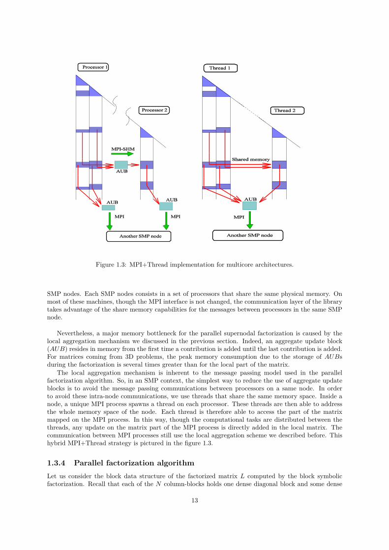
Figure 1.3: MPI+Thread implementation for multicore architectures.

SMP nodes. Each SMP nodes consists in a set of processors that share the same physical memory. Onmost of these machines, though the MPI interface is not changed, the communication layer of the librarytakes advantage of the share memory capabilities for the messages between processors in the same SMPnode.

Nevertheless, a major memory bottleneck for the parallel supernodal factorization is caused by thelocal aggregation mechanism we discussed in the previous section. Indeed, an aggregate update block(AUB) resides in memory from the first time a contribution is added until the last contribution is added.For matrices coming from 3D problems, the peak memory consumption due to the storage of AUBsduring the factorization is several times greater than for the local part of the matrix.

The local aggregation mechanism is inherent to the message passing model used in the parallelfactorization algorithm. So, in an SMP context, the simplest way to reduce the use of aggregate updateblocks is to avoid the message passing communications between processors on a same node. In orderto avoid these intra-node communications, we use threads that share the same memory space. Inside anode, a unique MPI process spawns a thread on each processor. These threads are then able to addressthe whole memory space of the node. Each thread is therefore able to access the part of the matrixmapped on the MPI process. In this way, though the computational tasks are distributed between thethreads, any update on the matrix part of the MPI process is directly added in the local matrix. Thecommunication between MPI processes still use the local aggregation scheme we described before. Thishybrid MPI+Thread strategy is pictured in the figure 1.3.

1.3.4 Parallel factorization algorithmLet us consider the block data structure of the factorized matrix L computed by the block symbolicfactorization. Recall that each of the N column-blocks holds one dense diagonal block and some dense

13

off-diagonal blocks. Then we define the two sets: BStruct(Lk∗) is the set of column-blocks that updatecolumn-block k, and BStruct(L∗k) is the set of column-blocks updated by column-block k (see [72, 73,74, 75] for details).

Let us now consider a parallel supernodal version of sparse factorization with total local aggregation:all non-local block contributions are aggregated locally in block structures. This scheme is close to theFan-In algorithm [19] as processors communicate using only aggregated update blocks. These aggregatedupdate blocks, denoted in what follows by AUB, can be built from the block symbolic factorization.These contributions are locally aggregated before being sent. The proposed algorithm can yield 1D(column-block) or 2D (block) distributions [72, 74].

The pseudo-code of LLT factorization can be expressed in terms of dense block computations ortasks; these computations are performed, as much as possible, on compacted sets of blocks for BLASefficiency.

Let us introduce the notation:

• τ : local thread number;

• π : local process number;

• Nτ : total number of tasks mapped on thread τ ;

• Kτ [i] : ith task of thread τ ;

• for the column-block k, symbol ? means ∀j ∈ BStruct(L∗k);

• let j ≥ k; sequence [j] means ∀i ∈ BStruct(L∗k) ∪ {k} with i ≥ j.

• map2process(, ) operator is the 2D block mapping function by process.

Block computations can be classified in four types, and the associated tasks are defined as follows:

• COMP1D(k) : factorize the column-block k and compute all the contributions for the column-blocksin BStruct(L∗k)

. Factorize Akk into LkkLtkk

. Solve LkkAt?k = At?k

. For j ∈ BStruct(L∗k) Do

. Compute C[j] = L[j]kAt?k

. If map2process([j], j) == π Then A[j]j = A[j]j − C[j]

. Else AUB[j]j = AUB[j]j + C[j]

• FACTOR(k) : factorize the diagonal block k

. Factorize Akk into LkkLtkk

• BDIV(j,k) : update the off-diagonal block j in column-block k

. Solve LkkAtjk = Atjk

• BMOD(i,j,k) : compute the contribution of the block i in column-block k for block i in column-blockj

. Compute Ci = LikAtjk

. If map2process(i, j) == π Then Aij = Aij − Ci

. Else AUBij = AUBij + Ci

On each thread τ , Kτ is the vector of tasks for computations (lines 2 on Figure 1.4), ordered bypriority. Each task should have received all its contributions and should have updated associated localdata before any new contribution is computed. When the last contribution is aggregated in the corre-sponding AUB, this aggregated update block is said to be “completely aggregated” and is ready to besent. To achieve a good efficiency, the sending of AUB has to match the static scheduling of tasks onthe destination processor.

14

1. For n = 1 to Nτ Do2. Switch ( Type(Kτ [n]) ) Do3. COMP1D: Receive all AUB[k]k for A[k]k4. COMP1D(k)5 If AUB[j],j is completed then send it to map2process(i,j)6. FACTOR: Receive all AUBkk for Akk

7. FACTOR(k)8. send LkkDk to map2process([k], k)9. BDIV: Receive Lkk and all AUBjk for Ajk

10. BDIV(j,k)11. send At

jk to map2process([j], k)12. BMOD: Receive At

jk

13. BMOD(i,j,k)14. If AUBi,j is completed then send it to map2process(i,j)

Figure 1.4: Outline of the parallel factorization algorithm.

1.3.5 Matrix mapping and task schedulingBefore running the general parallel algorithm presented above, we must perform a step consisting ofpartitioning and mapping the blocks of the symbolic matrix onto the set of SMP nodes. The partitioningand mapping phase aims at computing a static assignment that balances workload and enforces theprecedence constraints imposed by the factorization algorithm; the block elimination tree structure mustbe used there.

Our main algorithm is based on a static regulation led by a time simulation during the mappingphase. Thus, the partitioning and mapping step generates a fully ordered schedule used in the parallelfactorization. This schedule aims at statically regulating all of the issues that are classically managed atruntime. To make our scheme very reliable, we estimate the workload and message passing latency byusing a BLAS and communication network time model, which is automatically calibrated on the targetarchitecture.

Unlike usual algorithms, our partitioning and distribution strategy is divided in two distinct phases.The partition phase splits column-blocks associated with large supernodes, builds, for each column-block, a set of candidate threads for its mapping, and determines if it will be mapped using a 1D or2D distribution. Once the partitioning step is over, the task graph is built. In this graph, each taskis associated with the set of candidate threads of its column-block. The mapping and scheduling phasethen optimally maps each task onto one of these threads. An important constraint is that once a taskhas been mapped on a thread then all the data accessed by this thread are also mapped on the processassociated with the thread. This means that an unmapped task that accesses a block already mappedwill be necessarily mapped on the same process (i.e. SMP node).

The partitioning algorithm is based on a recursive top-down strategy over the block elimination treeprovided by block symbolic factorization. Pothen and Sun presented such a strategy in [121]. It startsby splitting the root and assigning it to a set of candidate threads Q that is the set of all threads. Giventhe number of candidate threads and the size of the supernodes, it chooses the strategy (1D or 2D) thatthe mapping and scheduling phase will use to distribute this supernode. Then each subtree is recursivelyassigned to a subset of Q proportionally to its workload.

Once the partitioning phase has built a new partition and the set of candidate threads for each task,the election of an owner thread for each task falls to the mapping and scheduling phase. The idea behindthis phase is to simulate parallel factorization as each mapping comes along. Thus, for each thread,we define a timer that will hold the current elapsed computation time, and a ready task heap. At agiven time, this task heap will contain all tasks that are not yet mapped, that have received all of theircontributions, and for which the thread is a candidate. The algorithm starts by mapping the leaves ofthe elimination tree (those which have only one candidate thread). After a task has been mapped, thenext task to be mapped is selected as follows: we take the first task of each ready task heap and choosethe one that comes from the lowest node in the elimination tree. The communication pattern of allthe contributions for a task depends on the already mapped tasks and on the candidate thread for theownership of this task. The task is mapped onto the candidate thread that will be able to compute itthe soonest.

15

As a conclusion about the partitioning and mapping phase, we can say that we obtain a strategythat allows us to take into account, in the mapping of task computations, all the phenomena that occurduring the parallel factorization. Thus we achieve a block computation and communication scheme thatdrives the parallel solver efficiently.

1.4 Reducing the memory footprint using partial agregationtechniques

In the previous section, we have presented a mapping and scheduling algorithm for clusters of SMPnodes and we have shown the benefits on performance of such strategies. In addition to the problemof runtime performance, another important aspect in the direct resolution of very large sparse systemsis the large memory requirement usually needed to factorize the matrix in parallel. A critical pointin industrial large-scaled application can be the memory overhead caused by the structures related tothe distributed data managment and the communications. These memory requirements can be causedby either the structures needed for communication (the AUB structures in our case) or by the matrixcœfficients themselves.

To deal with those problems of memory management, our statically scheduled factorization algorithmcan take advantage of the deterministic access (and allocation) pattern to all data stored in memory.Indeed the data access pattern is determined by the computational task ordering that drives the accessto the matrix coefficient blocks, and by the communication priorities that drive the access to the AUBstructures. We can consider two ways of using this predictable data access pattern:

• the first one consists in reducing the memory used to store the AUB by allowing some AUB stilluncompleted to be sent in order to temporarily free some memory. In this case, according toa memory limit fixed by the user, the AUB access pattern is used to determine which partiallyupdated AUB should be sent in advance to minimize the impact on the runtime performance;

• the second one is applied to an “out-of-core” version of the parallel factorization algorithm. In thiscase, according to a memory limit fixed by the user, we use the coefficient block access pattern toreduce the I/O volume and anticipate I/O calls.

In the case of the supernodal factorization with total aggregation of the contributions, this overhead ismainly due to the memory needed to store the AUB until they are entirely updated and sent. Indeed, anaggregated update block AUB is an overlapping block of all the contributions from a processor to a blockmapped on another processor. Hence an AUB structure is present in memory since the first contributionis added within and is released when it has been updated by its last contribution and actually sent.In some cases, particularly for matrices coming from 3D problems, the amount of memory needed forthe AUB still in memory can become important compared to the memory needed to store the matrixcœfficients.

A solution to address this problem is to reduce the number of AUBs simultaneously present in memory.Then, the technique consists in sending some AUBs partially updated before their actual completion andthen temporarily save some memory until the next contribution to be added in such AUB. This methodis called partial agregation [20].

The partial aggregation induces a time penalty compared to the total agregation due to more dynamicmemory reallocations and an increased volume of communications. Nevertheless, using the knowledgeof the AUB access pattern and the priority set on the messages, one can minimize this overhead.

Indeed by using the static scheduling, we are able to know, by following the ordered task vector andthe communication priorities, when an allocation or a deallocation will occur in the numerical factor-ization. That is to say that we are able to trace the memory consumption along the factorization taskswithout actually running it. Then, given a memory limit set by the user, the technique to minimize thenumber of partially updated AUBs needed to enforce this limitation is to choose some partially updatedAUBs among the AUBs in “memory” that will be updated again the later in the task vector. This isdone whenever this limit is overtaken in the logical traversal of the task vector.

16

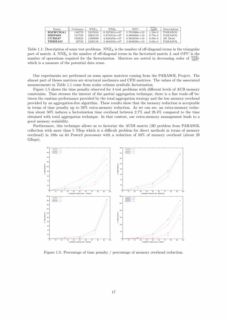
Name Columns NNZA NNZL OPC NNZLOPC Description

BMWCRA1 148770 5247616 6.597301e+07 5.701988e+10 1.16e-3 PARASOLSHIP003 121728 3982153 5.872912e+07 8.008089e+10 0.73e-3 PARASOLCUBE47 103823 1290898 4.828456e+07 6.963850e+10 0.69e-3 3D MeshTHREAD 29736 2220156 2.404333e+07 3.884020e+10 0.62e-3 PARASOL

Table 1.1: Description of some test problems. NNZA is the number of off-diagonal terms in the triangularpart of matrix A, NNZL is the number of off-diagonal terms in the factorized matrix L and OPC is thenumber of operations required for the factorization. Matrices are sorted in decreasing order of NNZL

OPCwhich is a measure of the potential data reuse.

Our experiments are performed on some sparse matrices coming from the PARASOL Project. Thealmost part of theses matrices are structural mechanics and CFD matrices. The values of the associatedmeasurements in Table 1.1 come from scalar column symbolic factorization.

Figure 1.5 shows the time penalty observed for 4 test problems with different levels of AUB memoryconstraints. That stresses the interest of the partial aggregation technique, there is a fine trade-off be-tween the runtime performance provided by the total aggregation strategy and the low memory overheadprovided by an aggregation-free algorithm. These results show that the memory reduction is acceptablein terms of time penalty up to 50% extra-memory reduction. As we can see, an extra-memory reduc-tion about 50% induces a factorization time overhead between 2.7% and 28.4% compared to the timeobtained with total aggregation technique. In that context, our extra-memory management leads to agood memory scalability.

Furthermore, this technique allows us to factorize the AUDI matrix (3D problem from PARASOLcollection with more than 5 Tflop which is a difficult problem for direct methods in terms of memoryoverhead) in 188s on 64 Power3 processors with a reduction of 50% of memory overhead (about 28Gflops).

0

20

40

60

80

100

120

140

160

180

0 10 20 30 40 50 60 70 80 90 100

% T

IME

PE

NA

LT

Y

% MEMORY REDUCTION THREAD

16 procs32 procs64 procs

128 procs

0

20

40

60

80

100

120

140

160

0 10 20 30 40 50 60 70 80 90 100

% T

IME

PE

NA

LT

Y

% MEMORY REDUCTION BMWCRA1

16 procs32 procs64 procs

128 procs

0

20

40

60

80

100

120

140

160

180

200

0 10 20 30 40 50 60 70 80 90 100

% T

IME

PE

NA

LT

Y

% MEMORY REDUCTION SHIP003

16 procs32 procs64 procs

128 procs

0

50

100

150

200

250

300

0 10 20 30 40 50 60 70 80 90 100

% T

IME

PE

NA

LT

Y

% MEMORY REDUCTION CUBE47

16 procs32 procs64 procs

128 procs

Figure 1.5: Percentage of time penalty / percentage of memory overhead reduction.

17

18

Chapter 2

Dynamic scheduling and runtimesystems

The first part of this chapter presents the work that has been developed in the PhD thesis of Math-ieu Faverge [48] (in french) that I have co-advised. Some contributions have been submitted to [49](according to the organizers, the proceedings have suffered many unfortunate delays due to extenuatingcircumstances, but will finally be published in two volumes, LNCS 6126 and 6127 in 2012).

The second part of this chapter presents the work that has been developed in the PhD thesis ofXavier Lacoste [95] (in english) that I have co-advised. Some contributions have been published in [96].

Please look at http://www.labri.fr/perso/ramet/restricted/HDR_HCW14.pdf for a full versionof this work with some experiments.

2.1 A dedicated approachNUMA (Non Uniform Memory Access) architectures have an important effect on memory access costs,and introduce contention problems which do not exist on SMP (Symmetric Multi-Processor) nodes.Thus, the main data structure of the sparse direct solver PaStiX has been modified to be more suitablefor NUMA architectures. A second modification, relying on overlapping opportunities, allows us to splitcomputational or communication tasks and to anticipate as much as possible the data receptions. Wealso introduce a simple way to dynamically schedule an application based on a dependency tree whiletaking into account NUMA effects. Results obtained with these modifications are illustrated by showingthe performance of the PaStiX solver on different platforms and matrices.

After a short description of architectures and matrices used for numerical experiments in Section 2.1.1,we study data allocation and mapping taking into account NUMA effects (see Section 2.1.2). Section 2.1.3focuses on the improvement of the communication overlap as preliminary work for a dynamic scheduler.Finally, a dynamic scheduler is described and evaluated on the PaStiX solver for various test cases inSections 2.1.4 and 2.1.5.

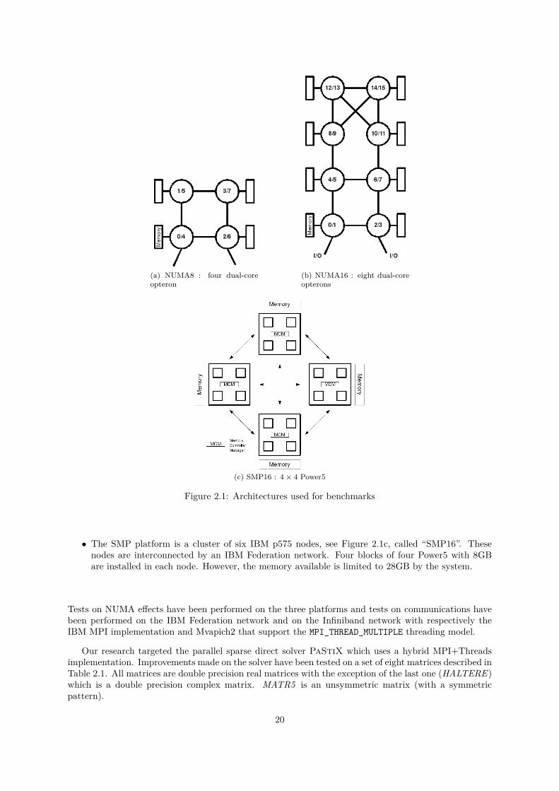
2.1.1 NUMA architecturesTwo NUMA and one SMP platforms have been used in this work :

• The first NUMA platform, see Figure 2.1a, denoted as “NUMA8”, is a cluster of ten nodes in-terconnected by an Infiniband network. Each node is made of four Dual-Core AMD Opteron(tm)processors interconnected by HyperTransport. The system memory amounts to 4GB per coregiving a total of 32GB.

• The second NUMA platform, see Figure 2.1b, called “NUMA16”, is a single node of eight Dual-CoreAMD Opteron(tm) processors with 64GB of memory.

19

(a) NUMA8 : four dual-coreopteron

(b) NUMA16 : eight dual-coreopterons

(c) SMP16 : 4× 4 Power5

Figure 2.1: Architectures used for benchmarks

• The SMP platform is a cluster of six IBM p575 nodes, see Figure 2.1c, called “SMP16”. Thesenodes are interconnected by an IBM Federation network. Four blocks of four Power5 with 8GBare installed in each node. However, the memory available is limited to 28GB by the system.

Tests on NUMA effects have been performed on the three platforms and tests on communications havebeen performed on the IBM Federation network and on the Infiniband network with respectively theIBM MPI implementation and Mvapich2 that support the MPI_THREAD_MULTIPLE threading model.

Our research targeted the parallel sparse direct solver PaStiX which uses a hybrid MPI+Threadsimplementation. Improvements made on the solver have been tested on a set of eight matrices described inTable 2.1. All matrices are double precision real matrices with the exception of the last one (HALTERE)which is a double precision complex matrix. MATR5 is an unsymmetric matrix (with a symmetricpattern).

20

Name Columns NNZA NNZL OPCMATR5 485 597 24 233 141 1 361 345 320 9.84422e+12AUDI 943 695 39 297 771 1 144 414 764 5.25815e+12NICE20 715 923 28 066 527 1 050 576 453 5.19123e+12INLINE 503 712 18 660 027 158 830 261 1.41273e+11NICE25 140 662 2 914 634 51 133 109 5.26701e+10MCHLNF 49 800 4 136 484 45 708 190 4.79105e+10THREAD 29 736 2 249 892 25 370 568 4.45729e+10HALTERE 1 288 825 10 476 775 405 822 545 7.62074e+11NNZA is the number of off-diagonal terms in the triangular part of the matrix A,NNZL is the number of off-diagonal terms in the factorized matrix L and OP C isthe number of operations required for the factorization.

Table 2.1: Matrices used for experiments

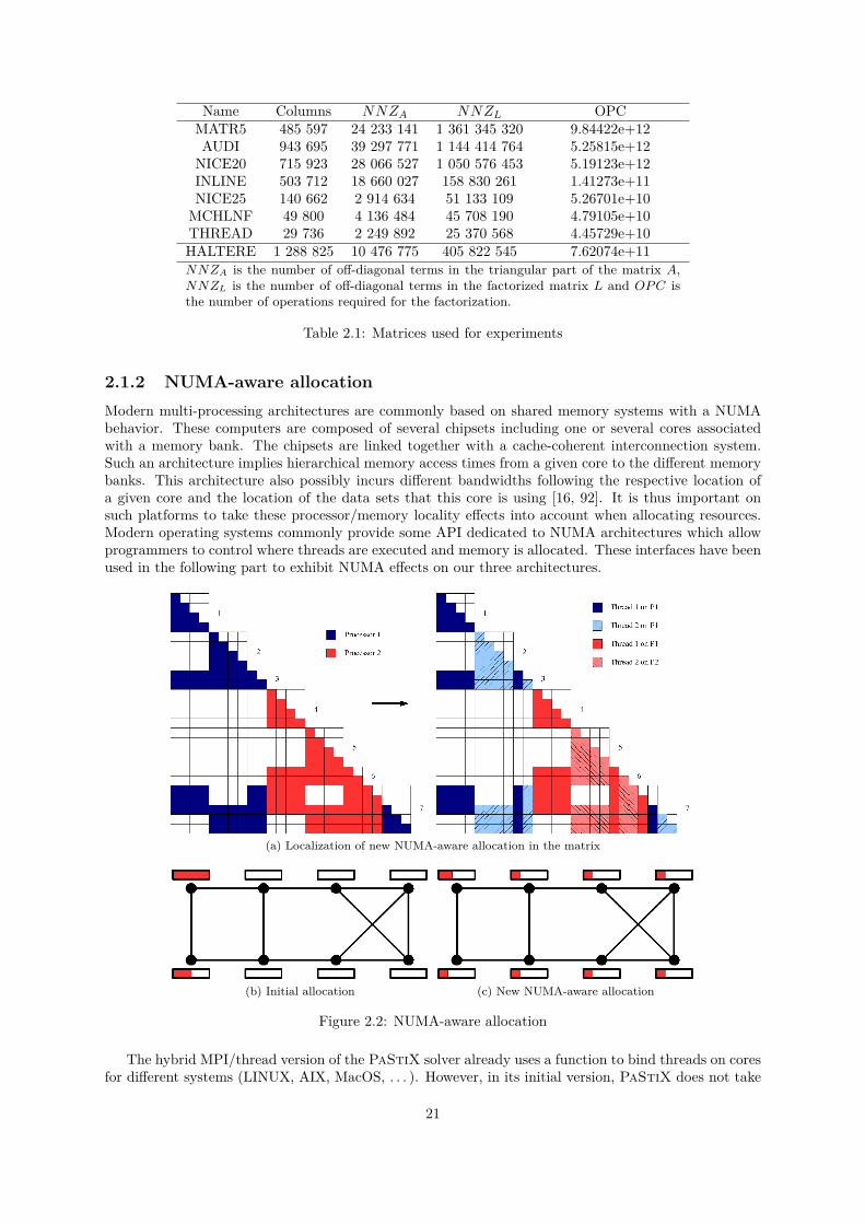
2.1.2 NUMA-aware allocationModern multi-processing architectures are commonly based on shared memory systems with a NUMAbehavior. These computers are composed of several chipsets including one or several cores associatedwith a memory bank. The chipsets are linked together with a cache-coherent interconnection system.Such an architecture implies hierarchical memory access times from a given core to the different memorybanks. This architecture also possibly incurs different bandwidths following the respective location ofa given core and the location of the data sets that this core is using [16, 92]. It is thus important onsuch platforms to take these processor/memory locality effects into account when allocating resources.Modern operating systems commonly provide some API dedicated to NUMA architectures which allowprogrammers to control where threads are executed and memory is allocated. These interfaces have beenused in the following part to exhibit NUMA effects on our three architectures.

(a) Localization of new NUMA-aware allocation in the matrix

(b) Initial allocation (c) New NUMA-aware allocation

Figure 2.2: NUMA-aware allocation

The hybrid MPI/thread version of the PaStiX solver already uses a function to bind threads on coresfor different systems (LINUX, AIX, MacOS, . . . ). However, in its initial version, PaStiX does not take

21

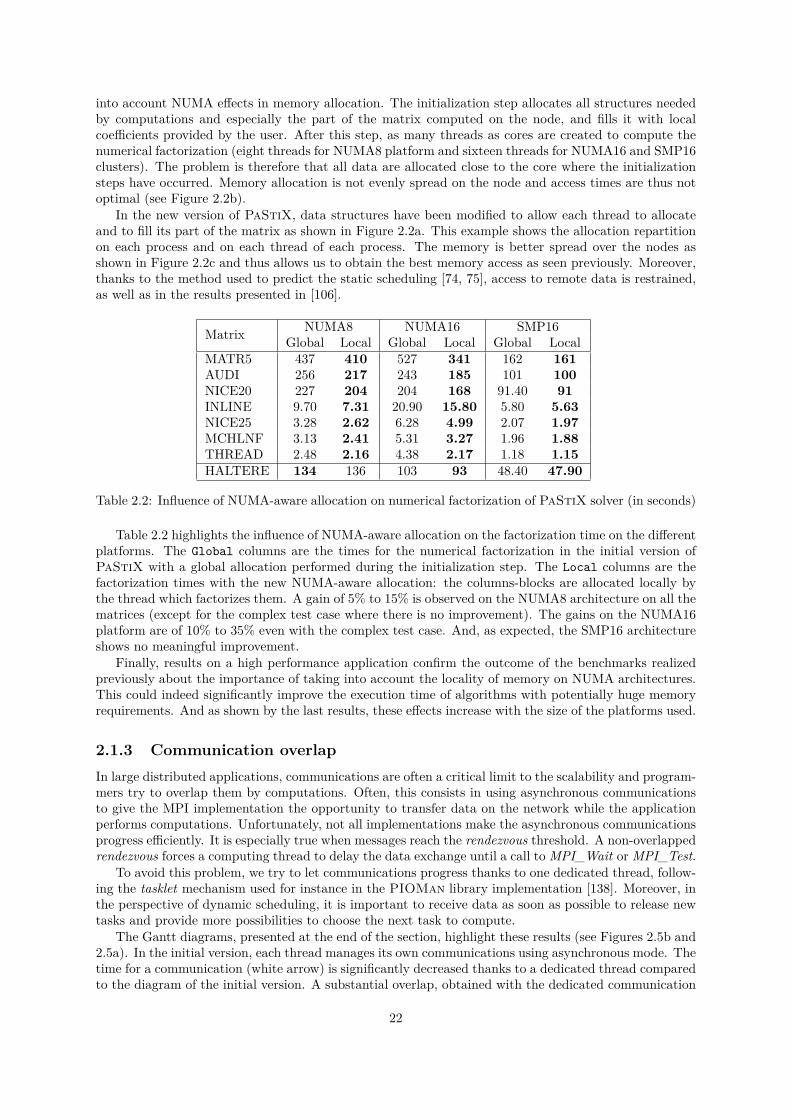
into account NUMA effects in memory allocation. The initialization step allocates all structures neededby computations and especially the part of the matrix computed on the node, and fills it with localcoefficients provided by the user. After this step, as many threads as cores are created to compute thenumerical factorization (eight threads for NUMA8 platform and sixteen threads for NUMA16 and SMP16clusters). The problem is therefore that all data are allocated close to the core where the initializationsteps have occurred. Memory allocation is not evenly spread on the node and access times are thus notoptimal (see Figure 2.2b).

In the new version of PaStiX, data structures have been modified to allow each thread to allocateand to fill its part of the matrix as shown in Figure 2.2a. This example shows the allocation repartitionon each process and on each thread of each process. The memory is better spread over the nodes asshown in Figure 2.2c and thus allows us to obtain the best memory access as seen previously. Moreover,thanks to the method used to predict the static scheduling [74, 75], access to remote data is restrained,as well as in the results presented in [106].

Matrix NUMA8 NUMA16 SMP16Global Local Global Local Global Local

MATR5 437 410 527 341 162 161AUDI 256 217 243 185 101 100NICE20 227 204 204 168 91.40 91INLINE 9.70 7.31 20.90 15.80 5.80 5.63NICE25 3.28 2.62 6.28 4.99 2.07 1.97MCHLNF 3.13 2.41 5.31 3.27 1.96 1.88THREAD 2.48 2.16 4.38 2.17 1.18 1.15HALTERE 134 136 103 93 48.40 47.90

Table 2.2: Influence of NUMA-aware allocation on numerical factorization of PaStiX solver (in seconds)

Table 2.2 highlights the influence of NUMA-aware allocation on the factorization time on the differentplatforms. The Global columns are the times for the numerical factorization in the initial version ofPaStiX with a global allocation performed during the initialization step. The Local columns are thefactorization times with the new NUMA-aware allocation: the columns-blocks are allocated locally bythe thread which factorizes them. A gain of 5% to 15% is observed on the NUMA8 architecture on all thematrices (except for the complex test case where there is no improvement). The gains on the NUMA16platform are of 10% to 35% even with the complex test case. And, as expected, the SMP16 architectureshows no meaningful improvement.

Finally, results on a high performance application confirm the outcome of the benchmarks realizedpreviously about the importance of taking into account the locality of memory on NUMA architectures.This could indeed significantly improve the execution time of algorithms with potentially huge memoryrequirements. And as shown by the last results, these effects increase with the size of the platforms used.

2.1.3 Communication overlapIn large distributed applications, communications are often a critical limit to the scalability and program-mers try to overlap them by computations. Often, this consists in using asynchronous communicationsto give the MPI implementation the opportunity to transfer data on the network while the applicationperforms computations. Unfortunately, not all implementations make the asynchronous communicationsprogress efficiently. It is especially true when messages reach the rendezvous threshold. A non-overlappedrendezvous forces a computing thread to delay the data exchange until a call to MPI_Wait or MPI_Test.

To avoid this problem, we try to let communications progress thanks to one dedicated thread, follow-ing the tasklet mechanism used for instance in the PIOMan library implementation [138]. Moreover, inthe perspective of dynamic scheduling, it is important to receive data as soon as possible to release newtasks and provide more possibilities to choose the next task to compute.

The Gantt diagrams, presented at the end of the section, highlight these results (see Figures 2.5b and2.5a). In the initial version, each thread manages its own communications using asynchronous mode. Thetime for a communication (white arrow) is significantly decreased thanks to a dedicated thread comparedto the diagram of the initial version. A substantial overlap, obtained with the dedicated communication

22

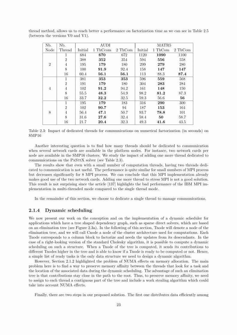
thread method, allows us to reach better a performance on factorization time as we can see in Table 2.5(between the versions V0 and V1).

Nb.Node

Nb.Thread

AUDI MATR5Initial 1 ThCcom 2 ThCom Initial 1 ThCom 2 ThCom

2

1 684 670 672 1120 1090 11002 388 352 354 594 556 5584 195 179 180 299 279 2808 100 91.9 92.4 158 147 14716 60.4 56.1 56.1 113 88.3 87.4

4

1 381 353 353 596 559 5682 191 179 180 304 283 2844 102 91.2 94.2 161 148 1508 55.5 48.3 54.9 98.2 81.2 87.316 33.7 32.2 32.5 59.3 56.6 56

8

1 195 179 183 316 290 3002 102 90.7 94 187 153 1644 56.4 47.1 50.7 93.7 78.8 1018 31.6 27.6 32.4 58.4 50 58.716 21.7 20.4 32.3 49.3 41.6 43.5

Table 2.3: Impact of dedicated threads for communications on numerical factorization (in seconds) onSMP16

Another interesting question is to find how many threads should be dedicated to communicationwhen several network cards are available in the platform nodes. For instance, two network cards pernode are available in the SMP16 clusters. We study the impact of adding one more thread dedicated tocommunications on the PaStiX solver (see Table 2.3).

The results show that even with a small number of computation threads, having two threads dedi-cated to communication is not useful. The performance is quite similar for small numbers of MPI processbut decreases significantly for 8 MPI process. We can conclude that this MPI implementation alreadymakes good use of the two network cards. Adding one more thread to stress MPI is not a good solution.This result is not surprising since the article [137] highlights the bad performance of the IBM MPI im-plementation in multi-threaded mode compared to the single thread mode.

In the remainder of this section, we choose to dedicate a single thread to manage communications.

2.1.4 Dynamic schedulingWe now present our work on the conception and on the implementation of a dynamic scheduler forapplications which have a tree shaped dependency graph, such as sparse direct solvers, which are basedon an elimination tree (see Figure 2.3a). In the following of this section, Tnode will denote a node of theelimination tree, and we will call Cnode a node of the cluster architecture used for computations. EachTnode corresponds to a column block to factorize and needs the updates from its descendants. In thecase of a right-looking version of the standard Cholesky algorithm, it is possible to compute a dynamicscheduling on such a structure. When a Tnode of the tree is computed, it sends its contributions todifferent Tnodes higher in the tree and is able to know if a Tnode is ready to be computed or not. Hence,a simple list of ready tasks is the only data structure we need to design a dynamic algorithm.

However, Section 2.1.2 highlighted the problem of NUMA effects on memory allocation. The mainproblem here is to find a way to preserve memory affinity between the threads that look for a task andthe location of the associated data during the dynamic scheduling. The advantage of such an eliminationtree is that contributions stay close in the path to the root. Thus, to preserve memory affinity, we needto assign to each thread a contiguous part of the tree and include a work stealing algorithm which couldtake into account NUMA effects.

Finally, there are two steps in our proposed solution. The first one distributes data efficiently among

23

all the Cnodes of the cluster. The second one builds a NUMA-aware dynamic scheduling on the localtasks mapped on each Cnode. We will now focus on the sparse direct linear solver PaStiX, which is ourtarget application for this work.

Sparse direct solver and static scheduling

In order to achieve efficient parallel sparse factorization, three preprocessing phases are commonly re-quired in direct sparse solvers (see Section 1.3).

In this work, we focus on the last preprocessing phase of the PaStiX solver, detailed in [74], thatcomputes a scheduling used during the numerical factorization phase. To build a static scheduling, firsta proportional mapping algorithm is applied on the processors of the target architecture. A BLAS2and/or BLAS3 time model gives weights for each column block in the elimination tree. Then, a recursivetop-down algorithm over the tree assigns a set of candidate processors to each Tnode (see Figure 2.3a).Processors chosen to compute a column block are assigned to its sons proportionally to the cost ofeach son and to the computations already affected to each candidate. It is possible to map the sameprocessor on two different branches to balance the computations on all available resources. The laststep corresponds to the data distribution over the Cnodes. A simulation of the numerical factorization isperformed thanks to an additional time model for communications. Thus, all tasks are mapped on one ofits candidates processors. Beforehand, tasks are sorted by priority based on the cost of the critical pathin the elimination tree. Then a greedy algorithm distributes tasks onto the candidates able to computeit the soonest. We obtain a vector of local tasks fully ordered by priority for each processor.

(a) First proportional mapping

(b) Second proportional mapping

Figure 2.3: Proportional mapping in elimination tree for static and dynamic scheduler.

This static scheduling gives very good results on most platforms. However we want to implementa dynamic scheduler at least as efficient as the static one, more suitable for NUMA or heterogeneousarchitectures. The objective is to reduce some observed idle times due to approximations in our timecost models, especially when communications have to be estimated. This is highlighted in Figure 2.5a.The other main objective is to preserve the memory affinity and locality particularly on architectureswith a large number of cores. Our static scheduling can be naturally adapted since all threads are bound

24

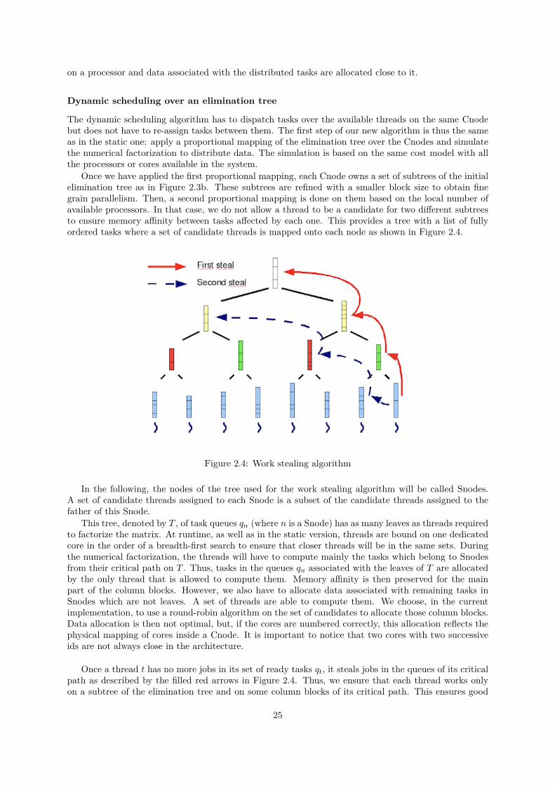
on a processor and data associated with the distributed tasks are allocated close to it.

Dynamic scheduling over an elimination tree

The dynamic scheduling algorithm has to dispatch tasks over the available threads on the same Cnodebut does not have to re-assign tasks between them. The first step of our new algorithm is thus the sameas in the static one: apply a proportional mapping of the elimination tree over the Cnodes and simulatethe numerical factorization to distribute data. The simulation is based on the same cost model with allthe processors or cores available in the system.

Once we have applied the first proportional mapping, each Cnode owns a set of subtrees of the initialelimination tree as in Figure 2.3b. These subtrees are refined with a smaller block size to obtain finegrain parallelism. Then, a second proportional mapping is done on them based on the local number ofavailable processors. In that case, we do not allow a thread to be a candidate for two different subtreesto ensure memory affinity between tasks affected by each one. This provides a tree with a list of fullyordered tasks where a set of candidate threads is mapped onto each node as shown in Figure 2.4.

Figure 2.4: Work stealing algorithm

In the following, the nodes of the tree used for the work stealing algorithm will be called Snodes.A set of candidate threads assigned to each Snode is a subset of the candidate threads assigned to thefather of this Snode.

This tree, denoted by T , of task queues qn (where n is a Snode) has as many leaves as threads requiredto factorize the matrix. At runtime, as well as in the static version, threads are bound on one dedicatedcore in the order of a breadth-first search to ensure that closer threads will be in the same sets. Duringthe numerical factorization, the threads will have to compute mainly the tasks which belong to Snodesfrom their critical path on T . Thus, tasks in the queues qn associated with the leaves of T are allocatedby the only thread that is allowed to compute them. Memory affinity is then preserved for the mainpart of the column blocks. However, we also have to allocate data associated with remaining tasks inSnodes which are not leaves. A set of threads are able to compute them. We choose, in the currentimplementation, to use a round-robin algorithm on the set of candidates to allocate those column blocks.Data allocation is then not optimal, but, if the cores are numbered correctly, this allocation reflects thephysical mapping of cores inside a Cnode. It is important to notice that two cores with two successiveids are not always close in the architecture.

Once a thread t has no more jobs in its set of ready tasks qt, it steals jobs in the queues of its criticalpath as described by the filled red arrows in Figure 2.4. Thus, we ensure that each thread works onlyon a subtree of the elimination tree and on some column blocks of its critical path. This ensures good

25

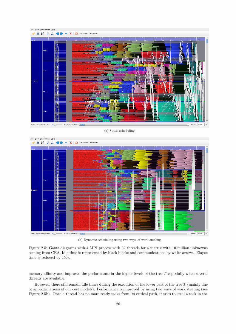
(a) Static scheduling

(b) Dynamic scheduling using two ways of work stealing

Figure 2.5: Gantt diagrams with 4 MPI process with 32 threads for a matrix with 10 million unknownscoming from CEA. Idle time is represented by black blocks and communications by white arrows. Elapsetime is reduced by 15%.

memory affinity and improves the performance in the higher levels of the tree T especially when severalthreads are available.

However, there still remain idle times during the execution of the lower part of the tree T (mainly dueto approximations of our cost models). Performance is improved by using two ways of work stealing (seeFigure 2.5b). Once a thread has no more ready tasks from its critical path, it tries to steal a task in the

26

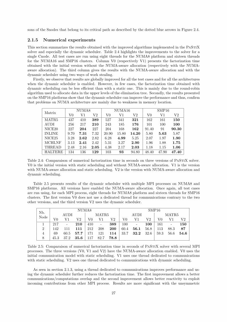
sons of the Snodes that belong to its critical path as described by the dotted blue arrows in Figure 2.4.

2.1.5 Numerical experimentsThis section summarizes the results obtained with the improved algorithms implemented in the PaStiXsolver and especially the dynamic scheduler. Table 2.4 highlights the improvements to the solver for asingle Cnode. All test cases are run using eight threads for the NUMA8 platform and sixteen threadsfor the NUMA16 and SMP16 clusters. Column V0 (respectively V1) presents the factorization timeobtained with the initial version without the NUMA-aware allocation (respectively with the NUMA-aware allocation). The third column gives the results with the NUMA-aware allocation and with thedynamic scheduler using two ways of work stealing.

Firstly, we observe that results are globally improved for all the test cases and for all the architectureswhen the dynamic scheduler is enabled. However, in few cases, the factorization time obtained withdynamic scheduling can be less efficient than with a static one. This is mainly due to the round-robinalgorithm used to allocate data in the upper levels of the elimination tree. Secondly, the results presentedon the SMP16 platforms show that the dynamic scheduler can improve the performance and thus, confirmthat problems on NUMA architecture are mainly due to weakness in memory location.

Matrix NUMA8 NUMA16 SMP16V0 V1 V2 V0 V1 V2 V0 V1 V2

MATR5 437 410 389 527 341 321 162 161 150AUDI 256 217 210 243 185 176 101 100 100NICE20 227 204 227 204 168 162 91.40 91 90.30INLINE 9.70 7.31 7.32 20.90 15.80 14.20 5.80 5.63 5.87NICE25 3.28 2.62 2.82 6.28 4.99 5.25 2.07 1.97 1.90MCHLNF 3.13 2.41 2.42 5.31 3.27 2.90 1.96 1.88 1.75THREAD 2.48 2.16 2.05 4.38 2.17 2.03 1.18 1.15 1.06HALTERE 134 136 129 103 93 94.80 48.40 47.90 47.40

Table 2.4: Comparaison of numerical factorization time in seconds on three versions of PaStiX solver.V0 is the initial version with static scheduling and without NUMA-aware allocation. V1 is the versionwith NUMA-aware allocation and static scheduling. V2 is the version with NUMA-aware allocation anddynamic scheduling.

Table 2.5 presents results of the dynamic scheduler with multiple MPI processes on NUMA8 andSMP16 platforms. All versions have enabled the NUMA-aware allocation. Once again, all test casesare run using, for each MPI process, eight threads for NUMA8 platform and sixteen threads for SMP16clusters. The first version V0 does not use a dedicated thread for communications contrary to the twoother versions, and the third version V2 uses the dynamic scheduler.

Nb.Node

NUMA8 SMP16AUDI MATR5 AUDI MATR5

V0 V1 V2 V0 V1 V2 V0 V1 V2 V0 V1 V21 217 - 210 410 - 389 100 - 100 161 - 1502 142 111 111 212 208 200 60.4 56.1 56.8 113 88.3 874 69 60.5 57.7 171 121 114 33.7 32.2 32.6 59.3 56.6 54.68 45.3 37.2 35.6 117 82.7 78.8

Table 2.5: Comparaison of numerical factorization time in seconds of PaStiX solver with several MPIprocesses. The three versions (V0, V1 and V2) have the NUMA-aware allocation enabled. V0 uses theinitial communication model with static scheduling. V1 uses one thread dedicated to communicationswith static scheduling. V2 uses one thread dedicated to communications with dynamic scheduling.

As seen in section 2.1.3, using a thread dedicated to communications improves performance and us-ing the dynamic scheduler further reduces the factorization time. The first improvement allows a bettercommunications/computations overlap and the second improvement allows better reactivity to exploitincoming contributions from other MPI process. Results are more significant with the unsymmetric

27

matrix MATR5, that generates more communications, than with symmetric matrices.

The improvements are mainly due to communications overlap and the gain obtained with the dynamicscheduler is about 5% on the factorization time. Even if our dynamic scheduler is not perfect, it alreadyimproves the hybrid MPI+Thread version of the PaStiX solver for all the platforms.

The NUMA-aware allocation implemented in the PaStiX solver gives very good results and canbe easily adapted to many applications. This points out that it is important to take care of memoryallocation during the initialization steps when using threads on NUMA architectures. Splitting commu-nication and computational tasks also achieves some improvements in connection with the communica-tion/computation overlap in the PaStiX solver. The work stealing algorithm can still be improved, butthe dynamic scheduler already improved the execution time for different test cases on platforms with orwithout a NUMA factor.

2.2 A generic approachEmerging processor technologies put an emphasis on increasing the number of computing units insteadof increasing their working frequencies. As a direct outcome of the physical multiplexing of hardwareresources, complex memory hierarchies have to be installed to reduce the memory bottleneck and ensurea decent rate of memory bandwidth for each resource. The memory becomes divided into several inde-pendent areas, capable of delivering data simultaneously through a complex and hierarchical topology,leading to the mainstream Non Uniform Memory Accesses (NUMA) machines we know today. To-gether with the availability of hardware accelerators, this trend profoundly altered the execution modelof current and future platforms, progressing them towards a scale and a complexity unattained before.Furthermore, with the established integration of accelerators into modern architectures, such as GPUsor Intel Xeon Phis, high-end multi-core CPUs are consistently outperformed by these novel, more inte-grated, architectures both in terms of data processing rate and memory bandwidth. As a consequence,the working environment of today’s application developers has evolved towards a multi-level massivelyparallel environment, where computation becomes cheap but data movements expensive, driving up theenergy cost and algorithmic overheads and complexities.

With the advent of APIs for GPU programming, such as CUDA or OpenCL, programming accelera-tors has been rapidly evolving in the past years, permanently bringing accelerators into the mainstream.Hence, GPUs are becoming a more and more attractive alternative to traditional CPUs, particularlyfor their more interesting cost-per-flop and watts-per-flop ratios. However, the availability of a particu-lar programming API only partially addresses the development of hybrid algorithms capable of takingadvantage of all computational resources available, including accelerators and CPUs. Extracting a sat-isfactory level of performance, out of such entangled architectures, remains a real challenge due to thelack of consistent programming models and tools to assess their performance. In order to efficientlyexploit current and future architectures, algorithm developers are required to expose a large amount ofparallelism, adapt their code to new architectures with different programming models, and finally, mapit efficiently on the heterogeneous resources. This is a gargantuan task for most developers as they donot possess the architectural knowledge necessary to mold their algorithms on the hardware capabilitiesin order to achieve good efficiency, and/or do not want to spend new efforts with every new generationof hardware.

A significant amount of research has been done on dense linear algebra, but sparse linear algebraon heterogeneous system is work in progress. Multiple reasons warrant this divergence, including theintrinsic algorithmic complexity and the highly irregular nature of the resulting problem, both in termsof memory accesses and computational intensities. Combined with the heterogeneous features of currentand future parallel architectures, this depicts an extremely complex software development field.

In this work, we advance the state-of-the-art in supernodal solvers by migrating PaStiX towards anew programming paradigm, one with a promise of efficiently handling hybrid execution environmentswhile abstracting the application from the hardware constraints. Many challenges have to be overcome,going from exposing the PaStiX algorithms using a task-based programming paradigm, to deliveringa level of task parallelism, granularity, and implementation allowing the runtime to efficiently schedulethe resulting, highly irregular tasks, in a way that minimizes the execution span. We exposed theoriginal algorithm using the concept of tasks, a self-contained computational entity, linked to the other

28

tasks by data dependencies. Specialized task-graph description formats were used in accordance withthe underlying runtime system (PaRSEC or StarPU). We provided specialized GPU-aware versionsfor some of the most compute intensive tasks, providing the runtimes with the opportunity to unrollthe graph of tasks on all available computing resources. The resulting software is, to the best of ourknowledge, the first implementation of a sparse direct solver with a supernodal method supportinghybrid execution environments composed of multi-cores and multi-GPUs. Based on these elements,we pursue the evaluation of the usability and the appeal of using a task-based runtime as a substratefor executing this particular type of algorithm, an extremely computationally challenging sparse directsolver. Furthermore, we take advantage of the integration of accelerators (GPUs in this context) withour supporting runtimes, to evaluate and understand the impact of this drastically novel portable wayof writing efficient and perennial algorithms. Since the runtime system offers a uniform programminginterface, disassociate from a specific set of hardware or low-level software entities, applications can takeadvantage of these uniform programming interfaces for ensuring their portability. Moreover, the exposedgraph of tasks allows the runtime system to apply specialized optimization techniques and minimizethe application’s time to solution by strategically mapping the tasks onto computing resources by usingstate-of-the-art scheduling strategies.

The rest of the section is organized as follows. We first introduce some related work in Section 2.2.1,followed by a description of the runtimes used in Section 2.2.2. Section 2.2.3 explains the implementationover the DAG schedulers with a preliminary study over multi-core architectures, followed by details on theextension to heterogeneous architectures. All choices are supported and validated by a set of experimentson a set of matrices with a wide range of characteristics in Section 2.2.4.

2.2.1 Related workThe dense linear algebra community has spent a great deal of effort to tackle the challenges raised bythe sharp increase in the number of computational resources. Due to their heavy computational cost,most of their algorithms are relatively simple to handle. Avoiding common pitfalls such as the “fork-join”parallelism, and expertly selecting the blocking factor, provide an almost straightforward way to increasethe parallelism and thus achieve better performance. Moreover, due to their natural load-balance, mostof the algorithms can be approached hierarchically, first at the node level, and then at the computationalresource level. In a shared memory context, one of the seminal papers [28] replaced the commonlyused LAPACK layout with one based on tiles/blocks. Using basic operations on these tiles exposesthe algorithms as a graph of tasks augmented with dependencies between them. In shared memory, thisapproach quickly generates a large number of ready tasks, while, in distributed memory, the dependenciesallow the removal of hard synchronizations. This idea leads to the design of new algorithms for variousalgebraic operations [29], now at the base of well-known software packages like PLASMA [1].

This idea is recurrent in almost all novel approaches surrounding the many-core revolution, spreadingoutside the boundaries of dense linear algebra. Looking at sparse linear algebra, the efforts were directedtowards improving the behavior of the existing solvers by taking into account both task and data affinityand relying on a two-level hybrid parallelization approach, mixing multithreading and message passing.Numerous solvers are now able to efficiently exploit the capabilities of these new platforms [49, 130]. Newsolvers have also been designed and implemented to address these new platforms. For them the chosenapproach follows the one for dense linear algebra, fine-grained parallelism, thread-based parallelization,and advanced data management to deal with complex memory hierarchies. Examples of this kind ofsolver are HSL [80] and SuperLU-MT [98] for sparse LU or Cholesky factorizations and SPQR [42] andqr_mumps [27] for sparse QR factorizations.

One commonly employed approach consists in reducing the granularity of computations and avoiding"fork-join" parallelism, as the scalability of this scheme suffers from an excessive amount of synchro-nization. Most of the related work focuses on intra-node parallelization with a shared memory parallelprogramming paradigm. To be more precise, thread based parallelization is widely used to tackle theperformance issues within a computing node. These concepts have been first introduced in the fieldof dense linear algebra computations [28] where the main idea was to replace the commonly used datalayout for dense matrices with one based on tiles/blocks and to write novel algorithms suited to thisnew data organization; by defining a task as the execution of an elementary operation on a tile andby expressing data dependencies among these tasks in a Directed Acyclic Graph (DAG), the number ofsynchronizations is drastically reduced in comparison with classical approaches (such as the LAPACK or

29

ScaLAPACK libraries) thanks to a dynamic data-flow parallel execution model. This idea leads to thedesign of new algorithms for various algebra operations [29, 123] now at the base of well known softwarepackages like PLASMA [1] and FLAME [139].

Due to their deeply hierarchical architecture, memory accesses of multi-core based platforms are notuniform. Therefore, if the data is not carefully laid out in memory and if access to it is not coherent,multithreaded software may incur heavy performance penalties. The efficiency of the algorithms dis-cussed above can be considerably improved by accurately placing data in memory and by employingtasks scheduling algorithms that aim at maximizing the locality of accesses. This has only been madepossible by the availability of tools such as hwloc [26] that allow the application to discover the hardwarearchitecture of the underlying system and take advantage of it in a portable way.

With the advent of accelerator-based platforms, a lot of attention has shifted towards extending themulti-core aware algorithms to fully exploit the huge potential of accelerators (mostly GPUs). Themain challenges raised by these heterogeneous platforms are mostly related to task granularity and datamanagement: although regular cores require fine granularity of data as well as computations, acceleratorssuch as GPUs need coarse-grain tasks. This inevitably introduces the need for identifying the parts of thealgorithm which are more suitable to be processed by accelerators. As for the multi-core case describedabove, the exploitation of this kind of platform was first considered in the context of dense linear algebraalgorithms.

Moreover, one constant becomes clear: a need for a portable layer that will insulate the algorithmsand their developers from the rapid hardware changes. Recently, this portability layer appeared underthe denomination of a task-based runtime. The algorithms are described as tasks with data dependenciesin-between, and the runtime systems are used to manage the tasks dynamically and schedule them onall available resources. These runtimes can be generic, like the two runtimes used in the context of thisstudy (StarPU [21] or PaRSEC [24]), or more specialized like QUARK [147]. These efforts resultedin the design of the DPLASMA library [23] on top of PaRSEC and the adaptation of the existingFLAME library [83]. On the sparse direct methods front, preliminary work has resulted in mono-GPUimplementations based on offloading parts of the computations to the GPU [56, 105, 148]. Due to itsvery good data locality, the multifrontal method is the main target of these approaches. The mainidea is to treat some parts of the task dependency graph entirely on the GPU. Therefore, the mainoriginality of these efforts is in the methods and algorithms used to decide whether or not a task can beprocessed on a GPU. In most cases, this was achieved through a threshold based criterion on the size ofthe computational tasks.

Concerning accelerator-based platforms for sparse direct solvers, a lot of attention has been recentlypaid to design new algorithms that can exploit the huge potential of GPUs. For a multifrontal sparsedirect solver, some preliminary work has been proposed in the community [56, 148], resulting in single-GPU implementations based on off-loading parts of the computations to the GPU. The main idea is totreat some parts of the task dependency graph entirely on the GPU. Therefore, the main originality ofthese efforts was in the methods and algorithms used to decide whether or not a task can be processed on aGPU. In most cases this was achieved through a threshold based criterion on the size of the computationaltasks. From the software point of view, most of these studies have only produced software prototypesand few sparse direct solvers exploiting GPUs have been made available to the users, most of them beingdeveloped by private software companies such as MatrixPro1, Acceleware2 and BCSLib-GPU3. As faras we know, there are no publications nor reports where the algorithmic choices are depicted. Recentprogress towards a multifrontal sparse QR factorization on GPUs have been presented in [41].

2.2.2 RuntimesIn our exploratory approach towards moving to a generic scheduler for PaStiX, we considered twodifferent runtimes: StarPU and PaRSEC. Both runtimes have been proven mature enough in thecontext of dense linear algebra, while providing two orthogonal approaches to task-based systems.

The PaRSEC [24] distributed runtime system is a generic data-flow engine supporting a task-basedimplementation targeting hybrid systems. Domain specific languages are available to expose a user-friendly interface to developers and allow them to describe their algorithm using high-level concepts.

1http://www.matrixprosoftware.com/2http://www.acceleware.com/matrix-solvers3http://www.boeing.com/phantom/bcslib/

30

This programming paradigm constructs an abridged representation of the tasks and their dependenciesas a graph of tasks – a structure agnostic to algorithmic subtleties, where all intrinsic knowledge aboutthe complexity of the underlying algorithm is extricated, and the only constraints remaining are anno-tated dependencies between tasks [39]. This symbolic representation, augmented with a specific datadistribution, is then mapped on a particular execution environment. This runtime system supports theuse of different types of accelerators, GPUs and Intel Xeon Phi, in addition to distributed multi-coreprocessors. Data are transferred between computational resources based on coherence protocols andcomputational needs, with emphasis on minimizing the unnecessary transfers. The resulting tasks aredynamically scheduled on the available resources following a data reuse policy mixed with different crite-ria for adaptive scheduling. The entire runtime system targets very fine grain tasks (order of magnitudeunder ten microseconds), with a flexible scheduling and adaptive policies to mitigate the effect of systemnoise and to take advantage of the algorithmic-inherent parallelism to minimize the execution span.

The experiment presented in this work takes advantage of a specialized domain specific languageof PaRSEC, designed for affine loops-based programming [23]. This specialized interface allows for adrastic reduction in the memory used by the runtime, as tasks do not exist until they are ready to beexecuted, and the concise representation of the task-graph allows for an easy and stateless explorationof the graph. In exchange for the memory saving, generating a task requires some extra computation,and lies in the critical path of the algorithm. The need for a window of visible tasks is then pointless,the runtime can explore the graph dynamically based on the ongoing state of the execution.

StarPU [21] is a runtime system aiming to allow programmers to exploit the computing power ofclusters of hybrid systems composed of CPUs and various accelerators (GPUs, Intel Xeon Phi, etc) whilerelieving them from the need to specially adapt their programs to the target machine and processingunits. The StarPU runtime supports a task-based programming model, where applications submitcomputational tasks, with CPU and/or accelerator implementations, and StarPU schedules these tasksand associated data transfers on available CPUs and accelerators. The data that a task manipulatesis automatically transferred among accelerators and the main memory in an optimized way (minimizeddata transfers, data prefetch, communication overlapped with computations, etc.), so that programmersare relieved of scheduling issues and technical details associated with these transfers. StarPU takesparticular care of scheduling tasks efficiently, by establishing performance models of the tasks throughon-line measurements, and then using well-known scheduling algorithms from the literature. In addition,it allows scheduling experts, such as compilers or computational library developers, to implement customscheduling policies in a portable fashion.

The differences between the two runtimes can be classified into two groups: conceptual and practicaldifferences. At the conceptual level the main differences between PaRSEC and StarPU are the tasksubmission process, the centralized scheduling, and the data movement strategy. PaRSEC uses itsown parameterized language to describe the DAG in comparison with the simple sequential submissionloops typically used with StarPU. Therefore, StarPU relies on a centralized strategy that analyzes,at runtime, the dependencies between tasks and schedules these tasks on the available resources. On thecontrary, through compile-time information, each computational unit of PaRSEC immediately releasesthe dependencies of the completed task solely using the local knowledge of the DAG. Finally, whilePaRSEC uses an opportunistic approach, the StarPU scheduling strategy exploits cost models of thecomputation and data movements to schedule tasks to the right resource (CPU or GPU) in order tominimize overall execution time. However, it does not have a data-reuse policy on CPU-shared memorysystems, resulting in lower efficiency when no GPUs are used, compared to the data-reuse heuristic ofPaRSEC. At the practical level, PaRSEC supports multiple streams to manage the CUDA devices,allowing partial overlap between computing tasks, maximizing the occupancy of the GPU. On the otherhand, StarPU allows data transfers directly between GPUs without going through central memory,potentially increasing the bandwidth of data transfers when data is needed by multiple GPUs.

JDF representation of a DAG

In PaRSEC, the data distribution and dependencies are specified using the Job Data Flow (JDF) format.Fig. 2.6 shows our JDF representation of the sparse Cholesky factorization using the tasks panel andgemm. The task gemm is based only on the block id parameter and computes internally the supernode(fcblk) in which to apply the update. On Line 2 of panel(j), cblknbr is the number of block columnsin the Cholesky factor. Once the j-th panel is factorized, the trailing submatrix can be updated using

31

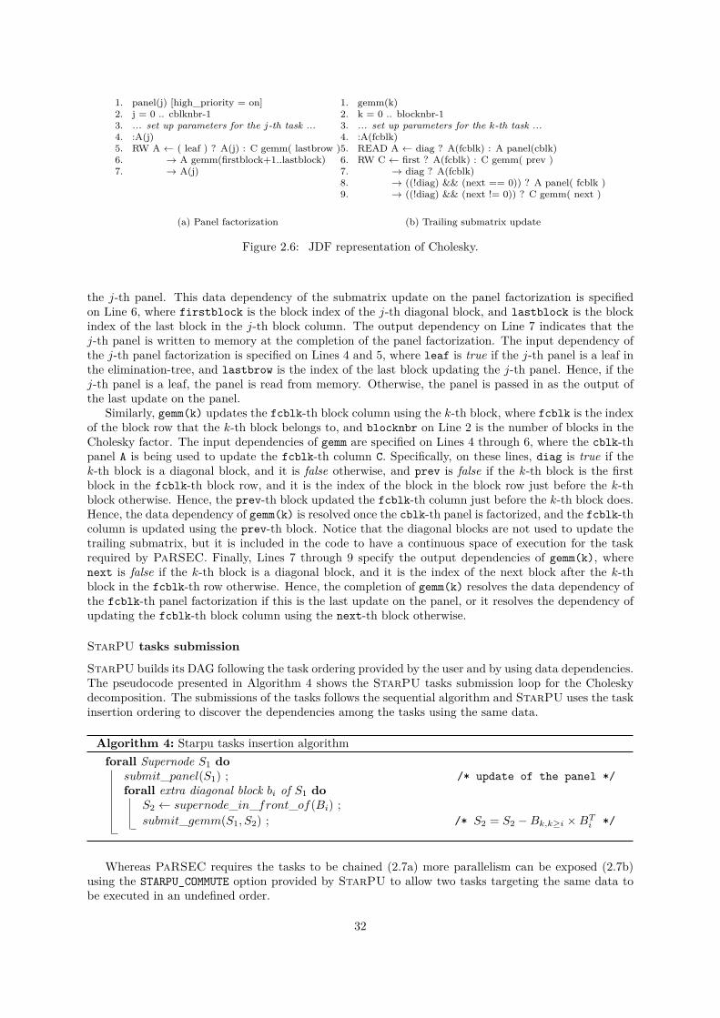
1. panel(j) [high_priority = on]2. j = 0 .. cblknbr-13. ... set up parameters for the j-th task ...4. :A(j)5. RW A ← ( leaf ) ? A(j) : C gemm( lastbrow )6. → A gemm(firstblock+1..lastblock)7. → A(j)

(a) Panel factorization

1. gemm(k)2. k = 0 .. blocknbr-13. ... set up parameters for the k-th task ...4. :A(fcblk)5. READ A ← diag ? A(fcblk) : A panel(cblk)6. RW C ← first ? A(fcblk) : C gemm( prev )7. → diag ? A(fcblk)8. → ((!diag) && (next == 0)) ? A panel( fcblk )9. → ((!diag) && (next != 0)) ? C gemm( next )

(b) Trailing submatrix update

Figure 2.6: JDF representation of Cholesky.

the j-th panel. This data dependency of the submatrix update on the panel factorization is specifiedon Line 6, where firstblock is the block index of the j-th diagonal block, and lastblock is the blockindex of the last block in the j-th block column. The output dependency on Line 7 indicates that thej-th panel is written to memory at the completion of the panel factorization. The input dependency ofthe j-th panel factorization is specified on Lines 4 and 5, where leaf is true if the j-th panel is a leaf inthe elimination-tree, and lastbrow is the index of the last block updating the j-th panel. Hence, if thej-th panel is a leaf, the panel is read from memory. Otherwise, the panel is passed in as the output ofthe last update on the panel.

Similarly, gemm(k) updates the fcblk-th block column using the k-th block, where fcblk is the indexof the block row that the k-th block belongs to, and blocknbr on Line 2 is the number of blocks in theCholesky factor. The input dependencies of gemm are specified on Lines 4 through 6, where the cblk-thpanel A is being used to update the fcblk-th column C. Specifically, on these lines, diag is true if thek-th block is a diagonal block, and it is false otherwise, and prev is false if the k-th block is the firstblock in the fcblk-th block row, and it is the index of the block in the block row just before the k-thblock otherwise. Hence, the prev-th block updated the fcblk-th column just before the k-th block does.Hence, the data dependency of gemm(k) is resolved once the cblk-th panel is factorized, and the fcblk-thcolumn is updated using the prev-th block. Notice that the diagonal blocks are not used to update thetrailing submatrix, but it is included in the code to have a continuous space of execution for the taskrequired by PaRSEC. Finally, Lines 7 through 9 specify the output dependencies of gemm(k), wherenext is false if the k-th block is a diagonal block, and it is the index of the next block after the k-thblock in the fcblk-th row otherwise. Hence, the completion of gemm(k) resolves the data dependency ofthe fcblk-th panel factorization if this is the last update on the panel, or it resolves the dependency ofupdating the fcblk-th block column using the next-th block otherwise.

StarPU tasks submission

StarPU builds its DAG following the task ordering provided by the user and by using data dependencies.The pseudocode presented in Algorithm 4 shows the StarPU tasks submission loop for the Choleskydecomposition. The submissions of the tasks follows the sequential algorithm and StarPU uses the taskinsertion ordering to discover the dependencies among the tasks using the same data.

Algorithm 4: Starpu tasks insertion algorithmforall Supernode S1 do

submit_panel(S1) ; /* update of the panel */forall extra diagonal block bi of S1 do

S2 ← supernode_in_front_of(Bi) ;submit_gemm(S1, S2) ; /* S2 = S2 −Bk,k≥i ×BTi */

Whereas PaRSEC requires the tasks to be chained (2.7a) more parallelism can be exposed (2.7b)using the STARPU_COMMUTE option provided by StarPU to allow two tasks targeting the same data tobe executed in an undefined order.

32

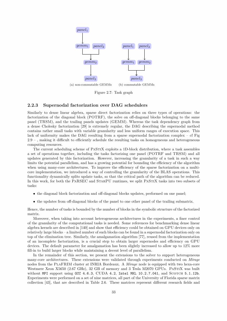
panel3

gemm2

gemm1

panel1

panel2

(a) non-commutable GEMMs

panel3

gemm1

panel1

gemm2

panel2

(b) commutable GEMMs

Figure 2.7: Task graph

2.2.3 Supernodal factorization over DAG schedulersSimilarly to dense linear algebra, sparse direct factorization relies on three types of operations: thefactorization of the diagonal block (POTRF), the solve on off-diagonal blocks belonging to the samepanel (TRSM), and the trailing panels updates (GEMM). Whereas the task dependency graph froma dense Cholesky factorization [29] is extremely regular, the DAG describing the supernodal methodcontains rather small tasks with variable granularity and less uniform ranges of execution space. Thislack of uniformity makes the DAG resulting from a sparse supernodal factorization complex – cf Fig2.9 – , making it difficult to efficiently schedule the resulting tasks on homogeneous and heterogeneouscomputing resources.

The current scheduling scheme of PaStiX exploits a 1D-block distribution, where a task assemblesa set of operations together, including the tasks factorizing one panel (POTRF and TRSM) and allupdates generated by this factorization. However, increasing the granularity of a task in such a waylimits the potential parallelism, and has a growing potential for bounding the efficiency of the algorithmwhen using many-core architectures. To improve the efficiency of the sparse factorization on a multi-core implementation, we introduced a way of controlling the granularity of the BLAS operations. Thisfunctionality dynamically splits update tasks, so that the critical path of the algorithm can be reduced.In this work, for both the PaRSEC and StarPU runtimes, we split PaStiX tasks into two subsets oftasks:

• the diagonal block factorization and off-diagonal blocks updates, performed on one panel;

• the updates from off-diagonal blocks of the panel to one other panel of the trailing submatrix.

Hence, the number of tasks is bounded by the number of blocks in the symbolic structure of the factorizedmatrix.

Moreover, when taking into account heterogeneous architectures in the experiments, a finer controlof the granularity of the computational tasks is needed. Some references for benchmarking dense linearalgebra kernels are described in [140] and show that efficiency could be obtained on GPU devices only onrelatively large blocks – a limited number of such blocks can be found in a supernodal factorization only ontop of the elimination tree. Similarly, the amalgamation algorithm [77], reused from the implementationof an incomplete factorization, is a crucial step to obtain larger supernodes and efficiency on GPUdevices. The default parameter for amalgamation has been slightly increased to allow up to 12% morefill-in to build larger blocks while maintaining a decent level of parallelism.

In the remainder of this section, we present the extensions to the solver to support heterogeneousmany-core architectures. These extensions were validated through experiments conducted on Miragenodes from the PlaFRIM cluster at INRIA Bordeaux. A Mirage node is equipped with two hexa-coreWestmere Xeon X5650 (2.67 GHz), 32 GB of memory and 3 Tesla M2070 GPUs. PaStiX was builtwithout MPI support using GCC 4.6.3, CUDA 4.2, Intel MKL 10.2.7.041, and Scotch 5.1.12b.Experiments were performed on a set of nine matrices, all part of the University of Florida sparse matrixcollection [43], that are described in Table 2.6. These matrices represent different research fields and

33

afshell10(D,

LU)

FilterV2(Z,

LU)Flan(D

,L

LT)audi(D

,L

LT)MHD(D

,L

U)

Geo1438(D

,L

LT)

pmlDF(Z,

LD

LT)

HOOK(D

,L

U)

Serena(D,

LD

LT)

0 20 40 60 80

Performance (GFlop/s)PaStiX

with

1core

StarPU

with

1core

PaRSE

Cwith

1core

PaStiXwith

3cores

StarPU

with

3cores

PaRSE

Cwith

3cores

PaStiXwith

6cores

StarPU

with

6cores

PaRSE

Cwith

6cores

PaStiXwith

9cores

StarPU

with

9cores

PaRSE

Cwith

9cores

PaStiXwith

12cores

StarPU

with

12cores

PaRSE

Cwith

12cores

Figure2.8:

CP

Uscaling

study:GFlop/s

performance

ofthefactorization

stepon

aset

ofninematrices

with

thethree

schedulers.

34

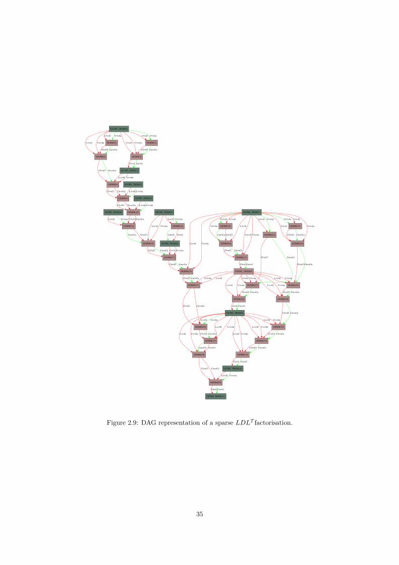
GETRF_TRSM(7)

GEMM(19)

L=>AlU=>Au

GEMM(20)

L=>AlU=>Au

GEMM(21)

L=>Al U=>Au GEMM(22)

L=>Al U=>Au

GEMM(23)

L=>AlU=>Au

GEMM(24)

L=>Al U=>Au

GEMM(25)

L=>Al U=>Au

Cl=>ClCu=>Cu

Cl=>Cl Cu=>Cu

GETRF_TRSM(8)

Cl=>LCu=>U

GEMM(27)

Cl=>Cl Cu=>Cu

Cl=>Cl Cu=>Cu

GEMM(29)

Cl=>Cl Cu=>Cu

GEMM(31)

Cl=>Cl Cu=>Cu L=>Al U=>Au

GEMM(28)

L=>Al U=>Au

L=>Al U=>Au

GEMM(30)

L=>Al U=>Au

L=>AlU=>Au

Cl=>Cl Cu=>Cu

GETRF_TRSM(9)

Cl=>L Cu=>U

Cl=>Cl Cu=>Cu

GEMM(33)

Cl=>Cl Cu=>Cu

GEMM(36)

Cl=>Cl Cu=>Cu

GETRF_TRSM(0)

GEMM(1)

L=>Al U=>Au

GEMM(2)

L=>Al U=>AuGEMM(3)

L=>Al U=>Au

GEMM(4)

L=>Al U=>Au

Cl=>Cl Cu=>Cu

GETRF_TRSM(1)

Cl=>L Cu=>U

Cl=>Cl Cu=>Cu

GEMM(6)

Cl=>Cl Cu=>Cu

L=>Al U=>Au

GEMM(8)

Cl=>Cl Cu=>Cu

GEMM(10)

Cl=>Cl Cu=>Cu

GETRF_TRSM(5)

GEMM(14)

L=>Al U=>Au

GEMM(15)

L=>Al U=>Au

GETRF_TRSM(6)

Cl=>LCu=>U

GEMM(17)

Cl=>Cl Cu=>Cu L=>Al U=>Au

Cl=>Cl Cu=>Cu

GETRF_TRSM(2)

L=>Al U=>Au

GEMM(12)

Cl=>Cl Cu=>Cu

GETRF_TRSM(3)

L=>Al U=>Au

Cl=>ClCu=>Cu

GETRF_TRSM(4)

L=>Al U=>Au

GEMM(37)

Cl=>Cl Cu=>Cu

L=>Al U=>Au L=>Al U=>Au

GEMM(34)

L=>Al U=>Au

GEMM(35)

L=>Al U=>Au

L=>Al U=>Au

GEMM(38)

L=>Al U=>Au Cl=>Cl Cu=>Cu

Cl=>Cl Cu=>Cu

GETRF_TRSM(10)

Cl=>L Cu=>U

Cl=>ClCu=>Cu

GEMM(40)

Cl=>Cl Cu=>Cu

GETRF_TRSM(11)

Cl=>LCu=>U

L=>Al U=>Au

Figure 2.9: DAG representation of a sparse LDLT factorisation.

35

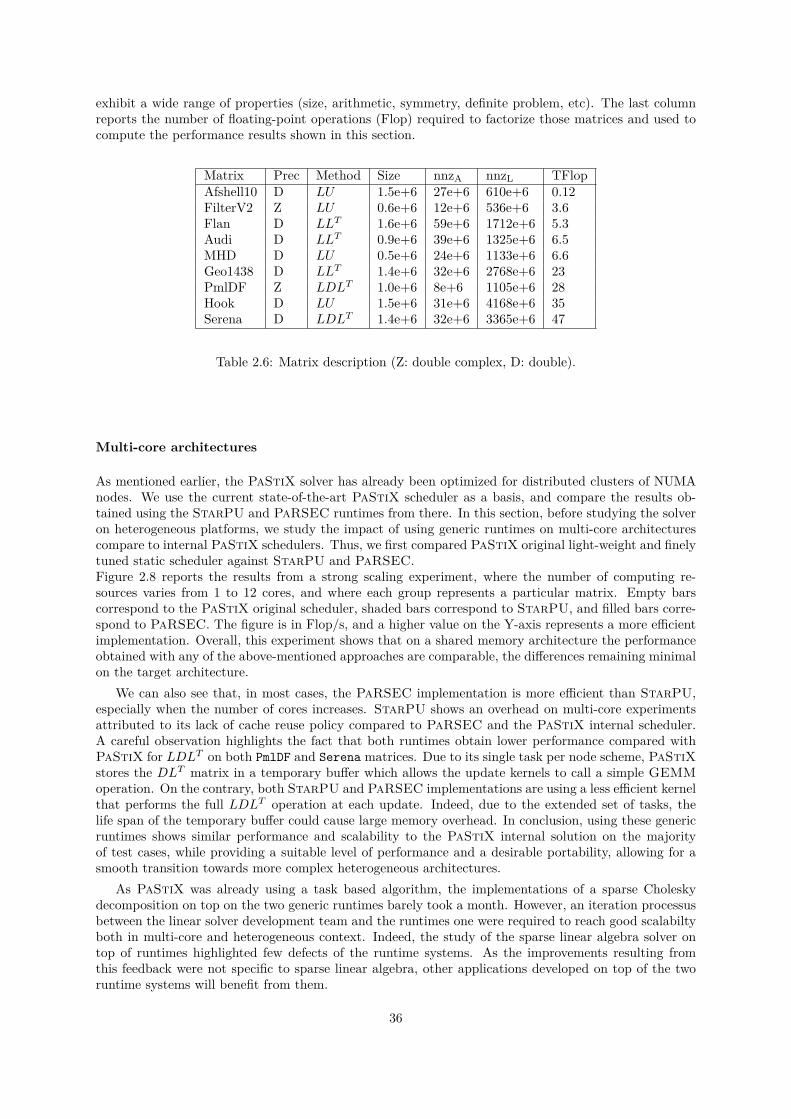
exhibit a wide range of properties (size, arithmetic, symmetry, definite problem, etc). The last columnreports the number of floating-point operations (Flop) required to factorize those matrices and used tocompute the performance results shown in this section.

Matrix Prec Method Size nnzA nnzL TFlopAfshell10 D LU 1.5e+6 27e+6 610e+6 0.12FilterV2 Z LU 0.6e+6 12e+6 536e+6 3.6Flan D LLT 1.6e+6 59e+6 1712e+6 5.3Audi D LLT 0.9e+6 39e+6 1325e+6 6.5MHD D LU 0.5e+6 24e+6 1133e+6 6.6Geo1438 D LLT 1.4e+6 32e+6 2768e+6 23PmlDF Z LDLT 1.0e+6 8e+6 1105e+6 28Hook D LU 1.5e+6 31e+6 4168e+6 35Serena D LDLT 1.4e+6 32e+6 3365e+6 47

Table 2.6: Matrix description (Z: double complex, D: double).

Multi-core architectures

As mentioned earlier, the PaStiX solver has already been optimized for distributed clusters of NUMAnodes. We use the current state-of-the-art PaStiX scheduler as a basis, and compare the results ob-tained using the StarPU and PaRSEC runtimes from there. In this section, before studying the solveron heterogeneous platforms, we study the impact of using generic runtimes on multi-core architecturescompare to internal PaStiX schedulers. Thus, we first compared PaStiX original light-weight and finelytuned static scheduler against StarPU and PaRSEC.Figure 2.8 reports the results from a strong scaling experiment, where the number of computing re-sources varies from 1 to 12 cores, and where each group represents a particular matrix. Empty barscorrespond to the PaStiX original scheduler, shaded bars correspond to StarPU, and filled bars corre-spond to PaRSEC. The figure is in Flop/s, and a higher value on the Y-axis represents a more efficientimplementation. Overall, this experiment shows that on a shared memory architecture the performanceobtained with any of the above-mentioned approaches are comparable, the differences remaining minimalon the target architecture.

We can also see that, in most cases, the PaRSEC implementation is more efficient than StarPU,especially when the number of cores increases. StarPU shows an overhead on multi-core experimentsattributed to its lack of cache reuse policy compared to PaRSEC and the PaStiX internal scheduler.A careful observation highlights the fact that both runtimes obtain lower performance compared withPaStiX for LDLT on both PmlDF and Serena matrices. Due to its single task per node scheme, PaStiXstores the DLT matrix in a temporary buffer which allows the update kernels to call a simple GEMMoperation. On the contrary, both StarPU and PaRSEC implementations are using a less efficient kernelthat performs the full LDLT operation at each update. Indeed, due to the extended set of tasks, thelife span of the temporary buffer could cause large memory overhead. In conclusion, using these genericruntimes shows similar performance and scalability to the PaStiX internal solution on the majorityof test cases, while providing a suitable level of performance and a desirable portability, allowing for asmooth transition towards more complex heterogeneous architectures.

As PaStiX was already using a task based algorithm, the implementations of a sparse Choleskydecomposition on top on the two generic runtimes barely took a month. However, an iteration processusbetween the linear solver development team and the runtimes one were required to reach good scalabiltyboth in multi-core and heterogeneous context. Indeed, the study of the sparse linear algebra solver ontop of runtimes highlighted few defects of the runtime systems. As the improvements resulting fromthis feedback were not specific to sparse linear algebra, other applications developed on top of the tworuntime systems will benefit from them.

36

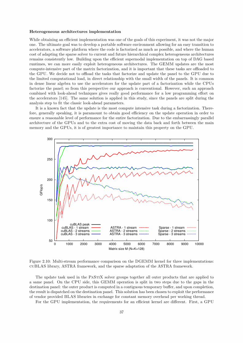
Heterogeneous architectures implementation

While obtaining an efficient implementation was one of the goals of this experiment, it was not the majorone. The ultimate goal was to develop a portable software environment allowing for an easy transition toaccelerators, a software platform where the code is factorized as much as possible, and where the humancost of adapting the sparse solver to current and future hierarchical complex heterogeneous architecturesremains consistently low. Building upon the efficient supernodal implementation on top of DAG basedruntimes, we can more easily exploit heterogeneous architectures. The GEMM updates are the mostcompute-intensive part of the matrix factorization, and it is important that these tasks are offloaded tothe GPU. We decide not to offload the tasks that factorize and update the panel to the GPU due tothe limited computational load, in direct relationship with the small width of the panels. It is commonin dense linear algebra to use the accelerators for the update part of a factorization while the CPUsfactorize the panel; so from this perspective our approach is conventional. However, such an approachcombined with look-ahead techniques gives really good performance for a low programming effort onthe accelerators [145]. The same solution is applied in this study, since the panels are split during theanalysis step to fit the classic look-ahead parameters.

It is a known fact that the update is the most compute intensive task during a factorization. There-fore, generally speaking, it is paramount to obtain good efficiency on the update operation in order toensure a reasonable level of performance for the entire factorization. Due to the embarrassingly parallelarchitecture of the GPUs and to the extra cost of moving the data back and forth between the mainmemory and the GPUs, it is of greatest importance to maintain this property on the GPU.

50

100

150

200

250

300

0 1000 2000 3000 4000 5000 6000 7000 8000 9000 10000

GF

lop/s

Matrix size M (N=K=128)

cuBLAS peakcuBLAS - 1 stream cuBLAS - 2 streamscuBLAS - 3 streams

ASTRA - 1 stream ASTRA - 2 streamsASTRA - 3 streams

Sparse - 1 stream Sparse - 2 streamsSparse - 3 streams

Figure 2.10: Multi-stream performance comparison on the DGEMM kernel for three implementations:cuBLAS library, ASTRA framework, and the sparse adaptation of the ASTRA framework.

The update task used in the PaStiX solver groups together all outer products that are applied toa same panel. On the CPU side, this GEMM operation is split in two steps due to the gaps in thedestination panel: the outer product is computed in a contiguous temporary buffer, and upon completion,the result is dispatched on the destination panel. This solution has been chosen to exploit the performanceof vendor provided BLAS libraries in exchange for constant memory overhead per working thread.

For the GPU implementation, the requirements for an efficient kernel are different. First, a GPU

37

has significantly less memory compared with what is available to a traditional processor, usually in therange of 3 to 6 GB. This forces us to carefully restrict the amount of extra memory needed during theupdate, making the temporary buffer used in the CPU version unsuitable. Second, the uneven nature ofsparse irregular matrices might limit the number of active computing units per task. As a result, onlya partial number of the available warps on the GPU might be active, leading to a deficient occupancy.Thus, we need the capability to submit multiple concurrent updates in order to provide the GPU driverwith the opportunity to overlap warps between different tasks to increase the occupancy, and thus theoverall efficiency.

Many CUDA implementations of the dense GEMM kernel are available to the scientific community.The most widespread implementation is provided by Nvidia itself in the cuBLAS library [114]. Thisimplementation is extremely efficient since CUDA 4.2 allows for calls on multiple streams, but is notopen source. Volkov developed an implementation for the first generation of CUDA enabled devices [140]in real single precision. In [136], the authors propose an assembly code of the DGEMM kernel thatprovides a 20% improvement on the cuBLAS 3.2 implementation. The MAGMA library proposeda first implementation of the DGEMM kernel [113] for the Nvidia Fermi GPUs. Later, an auto-tuned framework, called ASTRA, was presented in [94] and included in the MAGMA library. Thisimplementation, similar to the ATLAS library for CPUs, is a highly configurable skeleton with a set ofscripts to tune the parameters for each precision.

As our update operation is applied on a sparse representation of the panel and matrices, we cannotexploit an efficient vendor-provided GEMM kernel. We need to develop our own, starting from a denseversion and altering the algorithm to fit our needs. Due to the source code availability, the coverageof the four floating-point precisions, and it’s tuning capabilities, we decided to use the ASTRA-basedversion for our sparse implementation. As explained in [94] the matrix-matrix operation is performed intwo steps in this kernel. Each block of threads computes the outer-product tmp = AB into the GPUshared memory, and then the addition C = βC+αtmp is computed. To be able to compute directly intoC, the result of the update from one panel to another, we extended the kernel to provide the structure ofeach panel. This allows the kernel to compute the correct position directly into C during the sum step.This introduces a loss in the memory coalescence and deteriorates the update parts, however it preventsthe requirement of an extra buffer on the GPU for each offloaded kernel.

One problem in choosing the best parameters used in the MAGMA library for the ASTRA kernel isthat it has been determined that using textures gives the best performance for the update kernel. Thefunction cudaBindTexture and cudaUnbindTexture are not compatible with concurrent kernel calls ondifferent streams. Therefore, the textures have been disabled in the kernel, reducing the performance ofthe kernel by about 5% on large square matrices.

Figure 2.10 shows the study we made on the GEMM kernel and the impact of the modificationswe did on the ASTRA kernel. These experiments are done on a single GPU of the Mirage cluster.The experiments consist of computing a representative matrix-matrix multiplication of what is typicallyencountered during sparse factorization. Each point is the average performance of 100 calls to the kernelthat computes: C = C−ABT , with A, B, and C, matrices respectively of dimension M -by-N , K-by-N ,and M -by-N . B is taken as the first block of K rows of A as it is the case in Cholesky factorization.The plain lines are the performance of the cuBLAS library with 1 stream (red), 2 streams (green), and3 streams (red). The black line represents the peak performance obtained by the cuBLAS library onsquare matrices. This peak is never reached with the particular configuration case studied here. Thedashed lines are the performance of the ASTRA library in the same configuration. We observe thatthis implementation already loses 50GFlop/s, around 15%, against the cuBLAS library, and that mightbe caused by the parameters chosen by the auto-tuning framework which has been run only on squarematrices. Finally, the dotted lines illustrate the performance of the modified ASTRA kernel to includethe gaps into the C matrix. For the experiments, C is a panel twice as tall as A in which blocks arerandomly generated with average size of 200 rows. Blocks in A are also randomly generated with theconstraint that the rows interval of a block of A is included in the rows interval of one block of C, andno overlap is made between two blocks of A. We observe a direct relationship between the height of thepanel and the performance of the kernel: the taller the panel, the lower the performance of the kernel.The memory loaded to do the outer product is still the same as for the ASTRA curves, but memoryloaded for the C matrix grows twice as fast without increasing the number of Flop to perform. Theratio Flop per memory access is dropping and explains the decreasing performance. However, when thefactorization progresses and moves up the elimination trees, nodes get larger and the real number of

38

blocks encountered is smaller than the one used in this experiment to illustrate worst cases.Without regard to the kernel choice, it is important to notice how the multiple streams can have

a large impact on the average performance of the kernel. For this comparison, the 100 calls made inthe experiments are distributed in a round-robin manner over the available streams. One stream alwaysgives the worst performance. Adding a second stream increases the performance of all implementationsand especially for small cases when matrices are too small to feed all resources of the GPU. The thirdone is an improvement for matrices with M smaller than 1000, and is similar to two streams over 1000.

This kernel is the one we provide to both runtimes to offload computations on GPUs in the caseof Cholesky and LU factorizations. An extension to the kernel has been made to handle the LDLTfactorization that takes as an extra parameter the diagonal matrix D and computes: C = C − LDLT .This modified version decreases the performance by 5%.

Data mapping over multiple GPUs

We noticed that both runtimes encountered difficulties to compute the GEMM mapping onto the GPUs.Tasks’ irregularities – size of the GEMM block, Flop in the operation – complicates the prediction modelcalibration of StarPU to determine which process unit fits best for a task. Dynamic tasks mapping inPaRSEC could also result in a large unbalanced workload. Indeed in PaRSEC, the mapping of a panelto a given GPU enforces the mapping of all other tasks applied to the same panel, for the same reason asin StarPU, the irregularities in the task made it difficult for the simple model used in the dense case tocorrectly detect the actual load of each GPU. In order to help the runtime, panels that will be updatedon GPUs are selected at analyze time, such that the amount of data updated on a GPU does not exceedthe memory of the GPU. This limit will reduce the data transfer by keeping data on the GPUs. It isnecessary to sort the panels according to a criterion to decide in which ones will be mapped on a GPU.Several sorting criteria were tested: target panel’s size, the larger a panel is the more chance it has toreceive uploads; number of updates performed on the panel: this corresponds to the number of GEMMsapplied to the panel; Flop produced by these updates: not only the number of updates is important, butthe larger the updates are the more Flops will be performed; and, finally, the priority statically computedin PaStiX: higher is the priority, sooner the result is required, such that accelerators can help providingthem rapidly. Panels are marked to be updated on a specific GPU thanks to a greedy algorithm thatassociates at each step of the algorithm the first panel according to the selected criteria to the less loadedGPU. A check is made to guarantee we do not exceed the memory capacity of the GPU to avoid excessuse of the runtime LRU.

2.2.4 Heterogeneous experimentsFigure 2.11 presents the performance obtained on our set of matrices on the Mirage platform by enablingthe GPUs in addition to all available cores. The PaStiX run is shown as a reference. StarPU runsare empty bars, PaRSEC runs with 1 stream are shaded and PaRSEC runs with 3 streams are fullycolored. This experiment shows that we can efficiently use the additional computational power providedby the GPUs using the generic runtimes. In its current implementation, StarPU has either GPU orCPU worker threads. A GPU worker will execute only GPU tasks. Hence, when a GPU is used, aCPU worker is removed. With PaRSEC, no thread is dedicated to a GPU, and they all might executeCPU tasks as well as GPU tasks. The first computational thread that submits a GPU task takes themanagement of the GPU until no GPU work remains in the pipeline. Both runtimes manage to getsimilar performance and satisfying scalability over the 3 GPUs. In only two cases, MHD and pmlDF,StarPU outperforms PaRSEC results with 3 streams. This experiment also reveals that, as wasexpected, the computation takes advantage of the multiple streams that are available through PaRSEC.Indeed, the tasks generated by a sparse factorization are rather small and won’t use the entire GPU.This PaRSEC feature compensates for the prefetch strategy of StarPU that gave it the advantage whencompared to the one stream results. One can notice the poor performance obtained on the afshell testcase: in this case, the amount of Flop produced is too small to efficiently benefit from the GPUs.

Memory is a critical ressource for a direct solver. Figure 2.12 compares the memory peaks obtainedwith the three implementations of the solver, using eztrace. The runs where obtained with 12 coresbut the results would not be much different with an other setup.

The memory allocated cna be separated into five categories :

39

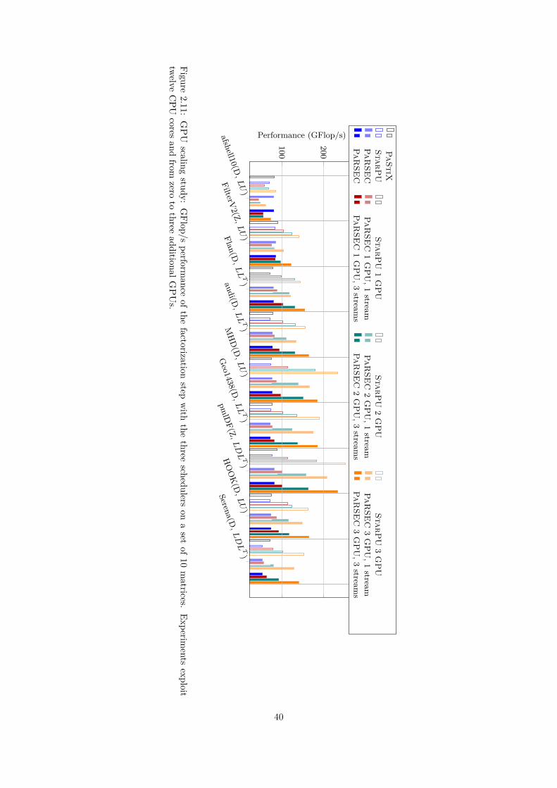
afshell10(D,

LU)

FilterV2(Z,

LU)Flan(D

,L

LT)audi(D

,L

LT)MHD(D

,L

U)

Geo1438(D

,L

LT)

pmlDF(Z,

LD

LT)

HOOK(D

,L

U)

Serena(D,

LD

LT)

100

200

Performance (GFlop/s)

PaStiXStarP

UStarP

U1

GP

UStarP

U2

GP

UStarP

U3

GP

UPaR

SEC

PaRSE

C1

GP

U,1

streamPaR

SEC

2G

PU,1

streamPaR

SEC

3G

PU,1

streamPaR

SEC

PaRSE

C1

GP

U,3

streams

PaRSE

C2

GP

U,3

streams

PaRSE

C3

GP

U,3

streams

Figure2.11:

GP

Uscaling

study:GFlop/s

performance

ofthe

factorizationstep

with

thethree

schedulerson

aset

of10

matrices.

Experiments

exploittw

elveCPU

coresand

fromzero

tothree

additionalGP

Us.

40

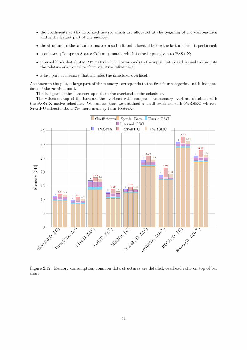
• the coefficients of the factorized matrix which are allocated at the begining of the compuataionand is the largest part of the memory;

• the structure of the factorized matrix also built and allocated before the factorization is performed;

• user’s CSC (Compress Sparse Column) matrix which is the imput given to PaStiX;

• internal block distributed CSC matrix which corresponds to the input matrix and is used to computethe relative error or to perform iterative refinement;

• a last part of memory that includes the scheduler overhead.

As shown in the plot, a large part of the memory corresponds to the first four categories and is indepen-dant of the runtime used.

The last part of the bars corresponds to the overhead of the scheduler.The values on top of the bars are the overhead ratio compared to memory overhead obtained with

the PaStiX native scheduler. We can see that we obtained a small overhead with PaRSEC whereasStarPU allocate about 7% more memory than PaStiX.

afshell10(D

, LU)

FilterV2(Z, LU)

Flan(D

, LLT )

audi(D,LLT )

MHD(D,LU

)

Geo1438(D

, LLT )

pmlDF(Z,LDLT )

HOOK

(D, LU)

Serena(D

, LDLT )0

5

10

15

20

25

30

35

2.8

1.7

2.2

1.330.67

1.39

1.41

1.65

1.24

3.613.1

3.45

3.292.97

3.29

4.01

4.45

3.93

11

1

11

1

1

1

1

Mem

ory

[GB

]

Coefficients Symb. Fact. User’s CSCInternal CSC

PaStiX StarPU PaRSEC

Figure 2.12: Memory consumption, common data structures are detailed, overhead ratio on top of barchart

41

42

Chapter 3

Incomplete factorization and domaindecomposition

The first part of this chapter presents the joint work with Pascal Hénon to implement an ILU(k)algorithm in the PaStiX solver [77].

Please look at http://www.labri.fr/perso/ramet/restricted/HDR_PC08.pdf for a full version ofthis work with some experiments.

The second part of this chapter presents work that has been developed in the PhD thesis of AstridCasadei [31] (in french) that I have co-advised. Some contributions have been published in [32].

Please look at http://www.labri.fr/perso/ramet/restricted/HDR_HIPC14.pdf for a full versionof this work with some experiments.

3.1 Amalgamation algorithm for iLU(k) factorizationSolving large sparse linear systems by iterative methods [129] has often been unsatisfactory when dealingwith practical “industrial" problems. The main difficulty encountered by such methods is their lack ofrobustness and, generally, the unpredictability and unconsistency of their performance when they areused over a wide range of different problems. Some methods can work quite well for certain types ofproblems but can fail on others. This has delayed their acceptance as “general-purpose” solvers in anumber of important applications.

Meanwhile, significant progress has been made in developing parallel direct methods for solving sparselinear systems, due in particular to advances made in both the combinatorial analysis of Gaussian elim-ination process, and on the design of parallel block solvers optimized for high-performance computers.For example, it is now possible to solve real-life three-dimensional problems with several million un-knowns, very effectively, with sparse direct solvers. This is achievable by a combination of state of theart algorithms along with careful implementations which exploit superscalar effects of the processors andother features of modern architectures [11, 64, 75, 76, 99]. However, direct methods will still fail tosolve very large three-dimensional problems, due to the potentially huge memory requirements for thesecases.

On the other hand, the iterative methods using a generic preconditioner like an ILU(k) factoriza-tion [129] require less memory, but they are often unsatisfactory when the simulation needs a solutionwith a good precision or when the systems are ill-conditioned. The incomplete factorization techniqueusually relies on a scalar implementation and thus does not benefit from the superscalar effects providedby the modern high performance architectures. Futhermore, these methods are difficult to parallelizeefficiently, more particulary for high values of level-of-fill. Some improvements to the classical scalarincomplete factorization have been studied to reduce the gap between the two classes of methods. In thecontext of domain decomposition, some algorithms that can be parallelized in an efficient way have beeninvestigated in [110]. In [124], the authors proposed to couple incomplete factorization with a selectiveinversion to replace the triangular solutions (that are not as scalable as the factorization) by scalablematrix-vector multiplications. The multifrontal method has also been adapted for incomplete factoriza-

43

tion with a threshold dropping in [89] or with a fill level dropping that measures the importance of anentry in terms of its updates [30]. In [34], the authors proposed a block ILU factorization technique forblock tridiagonal matrices.

The approach investigated in this work consists in exploiting the parallel blockwise algorithmic ap-proach used in the framework of high performance sparse direct solvers in order to develop robust parallelincomplete factorization based preconditioners [129] for iterative solvers. The idea is then to define anadaptive blockwise incomplete factorization that is much more efficient than the scalar incomplete fac-torizations commonly used to precondition iterative solvers. Indeed, by using the same ingredients whichmake direct solvers effective, these incomplete factorizations exploit the latest advances in sparse directmethods, and can be very competitive in terms of CPU time due to the effective usage of CPU power. Atthe same time, this approach can be far more economical in terms of memory usage than direct solvers.Therefore this should allow us to solve systems of much larger dimensions than those that are solved bythe direct solvers.

The section is organized as follows: Section 3.1.1 gives the principles of the block ILU factorizationbased on the level of fill, Section 3.1.2 presents our algorithms to obtain the approximate supernodepartition which aims at creating the sparse block structure of the incomplete factors and finally, inSection 3.1.3, we present some experiments obtained with our method.

3.1.1 MethodologyPreconditioned Krylov subspace methods utilize an accelerator and a preconditioner [129]. The goal ofthe ILU-based preconditioners is to find approximate LU factorizations of the coefficient matrix whichare then used to facilitate the iterative process.

Incomplete LU (ILU) or Incomplete Cholesky (IC) factorization are based on the premise that mostof the fill-in entries generated during a sparse direct factorization will tend to be small. Therefore, a fairlyaccurate factorization of A can be obtained by dropping most of the entries during the factorization.There are essentially two classical ways of developing incomplete LU factorizations.

The first (historically) consists of dropping terms according to a recursive definition of a level: a fill-inwhich is itself generated from another fill-in will tend to be smaller and smaller as this chain of creationcontinues. The notion of level-of-fill, first suggested by engineers is described next, as it is the steppingstone into the approach described in this work.

The second is based on the use of thresholds during the factorization. Thus, ILU(τ ,p) [128] is com-monly implemented as an upward-looking row-oriented algorithm which computes the ILU factorizationrow by row. It utilizes two parameters, the first τ being used as tolerance for dropping small termsrelative to the norm of the row under consideration, and the second p determines the maximum numberof nonzero elements to keep in each row.

ILU(k) preconditioners

The incomplete LU factorization ILU(k) implements dropping with the help of a level-of-fill associatedwith each fill-in introduced during the factorization. Initially, each nonzero element has a level-of-fill ofzero, while each zero element has (nominally) an infinite level-of-fill. Thereafter, the level-of-fill of lij isdefined from the formula:

levf (lij) = min{levf (lij); levf (lki) + levf (ljk) + 1} (3.1)

This definition and its justification were originally given by Watts for problems arising in petroleumengineering [142]. Later Forsyth and Tang provided a graph-based definition, which was then rein-terpreted by Hysom and Pothen [82] within the framework of the fill-path theorem [126]. The inter-pretation of the level-of-fill is that it is equal to len(i, j) − 1 where len is the length of the shortestfill-path between i and j. It can be easily seen that the path-lengths follow the simpler update rule:len(i, j) = min{len(i, j); len(i, k) + len(k, j)}. During Gaussian elimination, we eliminate nodes k, la-belled before a certain pair of nodes (i, j). Then, it can be proved that the shortest fill-path from i to jis the shortest of all shortest fill-paths from i to some k plus the shortest fill-path from k to j. This isillustrated in Figure (3.1).

The incomplete symbolic ILU(k) factorization has a theorical complexity similar to the numericalfactorization, but based on the graph interpretation of the level-of-fill, an efficient algorithm that leads

44

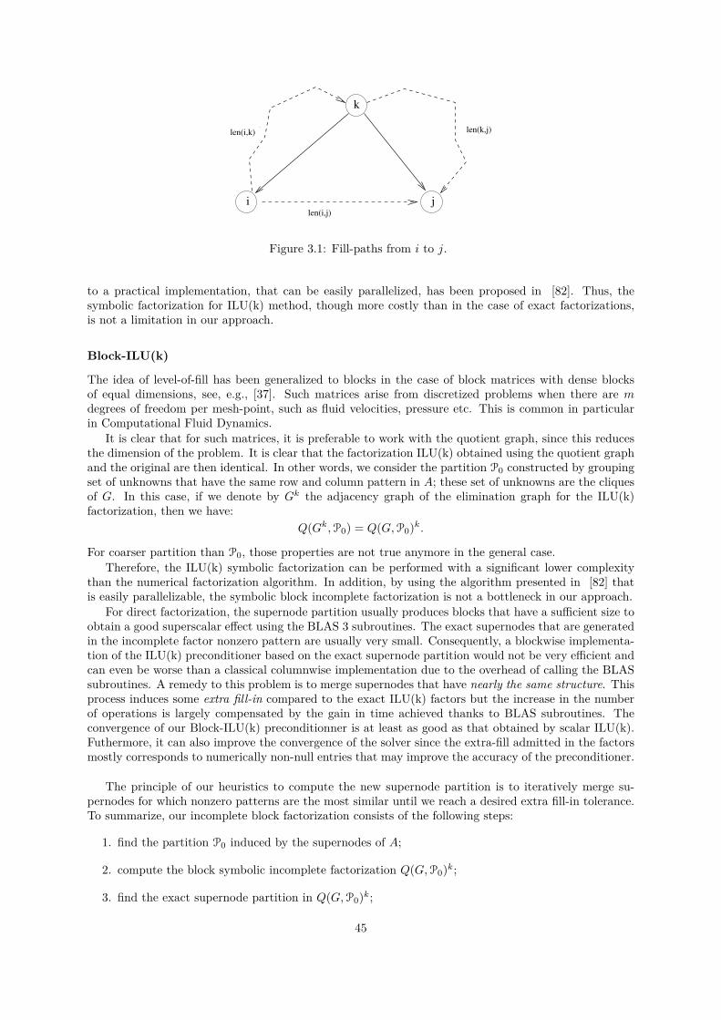
k

ji

len(i,k) len(k,j)

len(i,j)

Figure 3.1: Fill-paths from i to j.

to a practical implementation, that can be easily parallelized, has been proposed in [82]. Thus, thesymbolic factorization for ILU(k) method, though more costly than in the case of exact factorizations,is not a limitation in our approach.

Block-ILU(k)

The idea of level-of-fill has been generalized to blocks in the case of block matrices with dense blocksof equal dimensions, see, e.g., [37]. Such matrices arise from discretized problems when there are mdegrees of freedom per mesh-point, such as fluid velocities, pressure etc. This is common in particularin Computational Fluid Dynamics.

It is clear that for such matrices, it is preferable to work with the quotient graph, since this reducesthe dimension of the problem. It is clear that the factorization ILU(k) obtained using the quotient graphand the original are then identical. In other words, we consider the partition P0 constructed by groupingset of unknowns that have the same row and column pattern in A; these set of unknowns are the cliquesof G. In this case, if we denote by Gk the adjacency graph of the elimination graph for the ILU(k)factorization, then we have:

Q(Gk,P0) = Q(G,P0)k.

For coarser partition than P0, those properties are not true anymore in the general case.Therefore, the ILU(k) symbolic factorization can be performed with a significant lower complexity

than the numerical factorization algorithm. In addition, by using the algorithm presented in [82] thatis easily parallelizable, the symbolic block incomplete factorization is not a bottleneck in our approach.

For direct factorization, the supernode partition usually produces blocks that have a sufficient size toobtain a good superscalar effect using the BLAS 3 subroutines. The exact supernodes that are generatedin the incomplete factor nonzero pattern are usually very small. Consequently, a blockwise implementa-tion of the ILU(k) preconditioner based on the exact supernode partition would not be very efficient andcan even be worse than a classical columnwise implementation due to the overhead of calling the BLASsubroutines. A remedy to this problem is to merge supernodes that have nearly the same structure. Thisprocess induces some extra fill-in compared to the exact ILU(k) factors but the increase in the numberof operations is largely compensated by the gain in time achieved thanks to BLAS subroutines. Theconvergence of our Block-ILU(k) preconditionner is at least as good as that obtained by scalar ILU(k).Futhermore, it can also improve the convergence of the solver since the extra-fill admitted in the factorsmostly corresponds to numerically non-null entries that may improve the accuracy of the preconditioner.

The principle of our heuristics to compute the new supernode partition is to iteratively merge su-pernodes for which nonzero patterns are the most similar until we reach a desired extra fill-in tolerance.To summarize, our incomplete block factorization consists of the following steps:

1. find the partition P0 induced by the supernodes of A;

2. compute the block symbolic incomplete factorization Q(G,P0)k;

3. find the exact supernode partition in Q(G,P0)k;

45

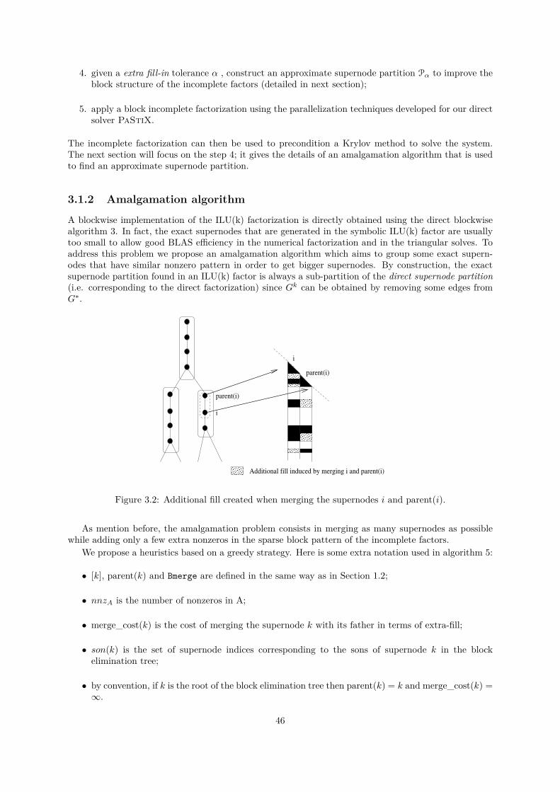
4. given a extra fill-in tolerance α , construct an approximate supernode partition Pα to improve theblock structure of the incomplete factors (detailed in next section);

5. apply a block incomplete factorization using the parallelization techniques developed for our directsolver PaStiX.

The incomplete factorization can then be used to precondition a Krylov method to solve the system.The next section will focus on the step 4; it gives the details of an amalgamation algorithm that is usedto find an approximate supernode partition.

3.1.2 Amalgamation algorithm

A blockwise implementation of the ILU(k) factorization is directly obtained using the direct blockwisealgorithm 3. In fact, the exact supernodes that are generated in the symbolic ILU(k) factor are usuallytoo small to allow good BLAS efficiency in the numerical factorization and in the triangular solves. Toaddress this problem we propose an amalgamation algorithm which aims to group some exact supern-odes that have similar nonzero pattern in order to get bigger supernodes. By construction, the exactsupernode partition found in an ILU(k) factor is always a sub-partition of the direct supernode partition(i.e. corresponding to the direct factorization) since Gk can be obtained by removing some edges fromG∗.

������������

������������

���������

���������

������

������

����������

����������

��������

��������

parent(i)

i

parent(i)

Additional fill induced by merging i and parent(i)

i

Figure 3.2: Additional fill created when merging the supernodes i and parent(i).

As mention before, the amalgamation problem consists in merging as many supernodes as possiblewhile adding only a few extra nonzeros in the sparse block pattern of the incomplete factors.

We propose a heuristics based on a greedy strategy. Here is some extra notation used in algorithm 5:

• [k], parent(k) and Bmerge are defined in the same way as in Section 1.2;

• nnzA is the number of nonzeros in A;

• merge_cost(k) is the cost of merging the supernode k with its father in terms of extra-fill;

• son(k) is the set of supernode indices corresponding to the sons of supernode k in the blockelimination tree;

• by convention, if k is the root of the block elimination tree then parent(k) = k and merge_cost(k) =∞.

46

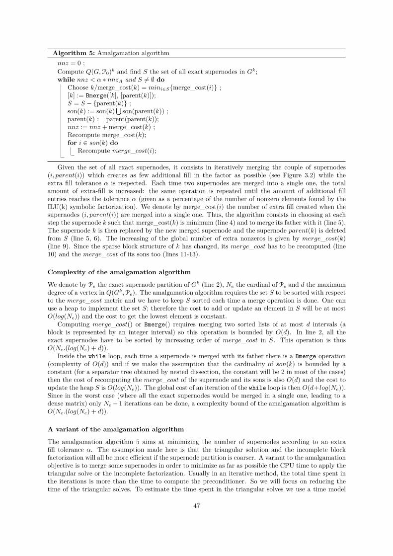
Algorithm 5: Amalgamation algorithmnnz = 0 ;Compute Q(G,P0)k and find S the set of all exact supernodes in Gk;while nnz < α ∗ nnzA and S 6= ∅ do

Choose k/merge_cost(k) = mini∈S{merge_cost(i)} ;[k] := Bmerge([k], [parent(k)]);S = S − {parent(k)} ;son(k) := son(k)

⋃son(parent(k)) ;

parent(k) := parent(parent(k));nnz := nnz + merge_cost(k) ;Recompute merge_cost(k);for i ∈ son(k) do

Recompute merge_cost(i);

Given the set of all exact supernodes, it consists in iteratively merging the couple of supernodes(i, parent(i)) which creates as few additional fill in the factor as possible (see Figure 3.2) while theextra fill tolerance α is respected. Each time two supernodes are merged into a single one, the totalamount of extra-fill is increased: the same operation is repeated until the amount of additional fillentries reaches the tolerance α (given as a percentage of the number of nonzero elements found by theILU(k) symbolic factorization). We denote by merge_cost(i) the number of extra fill created when thesupernodes (i, parent(i)) are merged into a single one. Thus, the algorithm consists in choosing at eachstep the supernode k such that merge_cost(k) is minimum (line 4) and to merge its father with it (line 5).The supernode k is then replaced by the new merged supernode and the supernode parent(k) is deletedfrom S (line 5, 6). The increasing of the global number of extra nonzeros is given by merge_cost(k)(line 9). Since the sparse block structure of k has changed, its merge_cost has to be recomputed (line10) and the merge_cost of its sons too (lines 11-13).

Complexity of the amalgamation algorithm

We denote by Pe the exact supernode partition of Gk (line 2), Ne the cardinal of Pe and d the maximumdegree of a vertex in Q(Gk,Pe). The amalgamation algorithm requires the set S to be sorted with respectto the merge_cost metric and we have to keep S sorted each time a merge operation is done. One canuse a heap to implement the set S; therefore the cost to add or update an element in S will be at mostO(log(Ne)) and the cost to get the lowest element is constant.

Computing merge_cost() or Bmerge() requires merging two sorted lists of at most d intervals (ablock is represented by an integer interval) so this operation is bounded by O(d). In line 2, all theexact supernodes have to be sorted by increasing order of merge_cost in S. This operation is thusO(Ne.(log(Ne) + d)).

Inside the while loop, each time a supernode is merged with its father there is a Bmerge operation(complexity of O(d)) and if we make the assumption that the cardinality of son(k) is bounded by aconstant (for a separator tree obtained by nested dissection, the constant will be 2 in most of the cases)then the cost of recomputing the merge_cost of the supernode and its sons is also O(d) and the cost toupdate the heap S is O(log(Ne)). The global cost of an iteration of the while loop is then O(d+log(Ne)).Since in the worst case (where all the exact supernodes would be merged in a single one, leading to adense matrix) only Ne− 1 iterations can be done, a complexity bound of the amalgamation algorithm isO(Ne.(log(Ne) + d)).

A variant of the amalgamation algorithm

The amalgamation algorithm 5 aims at minimizing the number of supernodes according to an extrafill tolerance α. The assumption made here is that the triangular solution and the incomplete blockfactorization will all be more efficient if the supernode partition is coarser. A variant to the amalgamationobjective is to merge some supernodes in order to minimize as far as possible the CPU time to apply thetriangular solve or the incomplete factorization. Usually in an iterative method, the total time spent inthe iterations is more than the time to compute the preconditioner. So we will focus on reducing thetime of the triangular solves. To estimate the time spent in the triangular solves we use a time model

47

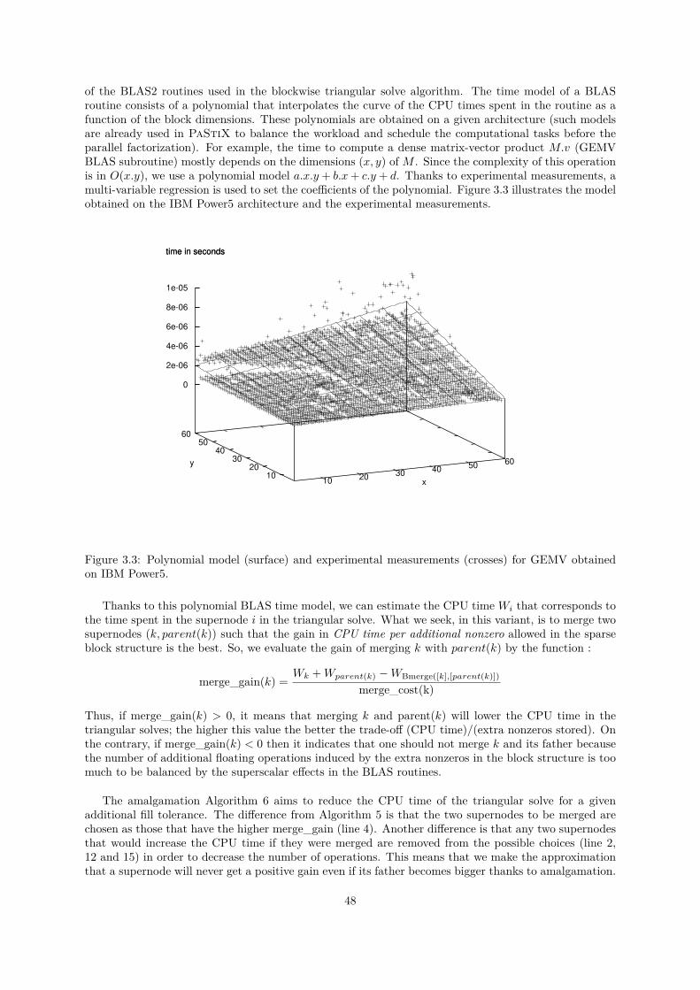
of the BLAS2 routines used in the blockwise triangular solve algorithm. The time model of a BLASroutine consists of a polynomial that interpolates the curve of the CPU times spent in the routine as afunction of the block dimensions. These polynomials are obtained on a given architecture (such modelsare already used in PaStiX to balance the workload and schedule the computational tasks before theparallel factorization). For example, the time to compute a dense matrix-vector product M.v (GEMVBLAS subroutine) mostly depends on the dimensions (x, y) of M . Since the complexity of this operationis in O(x.y), we use a polynomial model a.x.y + b.x+ c.y + d. Thanks to experimental measurements, amulti-variable regression is used to set the coefficients of the polynomial. Figure 3.3 illustrates the modelobtained on the IBM Power5 architecture and the experimental measurements.

10 20 30 40 50 60

10 20

30 40

50 60

0

2e-06

4e-06

6e-06

8e-06

1e-05

time in seconds

x

y

time in seconds

Figure 3.3: Polynomial model (surface) and experimental measurements (crosses) for GEMV obtainedon IBM Power5.

Thanks to this polynomial BLAS time model, we can estimate the CPU time Wi that corresponds tothe time spent in the supernode i in the triangular solve. What we seek, in this variant, is to merge twosupernodes (k, parent(k)) such that the gain in CPU time per additional nonzero allowed in the sparseblock structure is the best. So, we evaluate the gain of merging k with parent(k) by the function :

merge_gain(k) =Wk +Wparent(k) −WBmerge([k],[parent(k)])

merge_cost(k)

Thus, if merge_gain(k) > 0, it means that merging k and parent(k) will lower the CPU time in thetriangular solves; the higher this value the better the trade-off (CPU time)/(extra nonzeros stored). Onthe contrary, if merge_gain(k) < 0 then it indicates that one should not merge k and its father becausethe number of additional floating operations induced by the extra nonzeros in the block structure is toomuch to be balanced by the superscalar effects in the BLAS routines.

The amalgamation Algorithm 6 aims to reduce the CPU time of the triangular solve for a givenadditional fill tolerance. The difference from Algorithm 5 is that the two supernodes to be merged arechosen as those that have the higher merge_gain (line 4). Another difference is that any two supernodesthat would increase the CPU time if they were merged are removed from the possible choices (line 2,12 and 15) in order to decrease the number of operations. This means that we make the approximationthat a supernode will never get a positive gain even if its father becomes bigger thanks to amalgamation.

48

In practice, this approximation is verified most of the time according to the BLAS model we obtained.Algorithm 6: Amalgamation algorithm variantnnz = 0 ;Compute Q(G,P0)k and find S the set of all exact supernodes in Gk that have amerge_gain > 0;while nnz < α ∗ nnzA and S 6= ∅ do

Choose k/merge_gain(k) = maxi∈S{merge_gain(i)} ;[k] := Bmerge([k], [parent(k)]);S = S − {parent(k)} ;son(k) := son(k)

⋃son(parent(k)) ;

parent(k) := parent(parent(k));Compute merge_cost(k);nnz := nnz + merge_cost(k) ;Recompute merge_gain(k);if merge_gain(k) ≤ 0 then S = S − {k};;for i ∈ son(k) do

Recompute merge_gain(i);if merge_gain(i) ≤ 0 then S = S − {i};;

In the case of Algorithm 5, if we set α = ∞ then it would merge all the supernodes and the sparsematrix L (resp. U) would be considered as a dense matrix. An interesting property of Algorithm 6 isthat if we set α =∞ then it stops as soon as it cannot find any amalgamation of supernodes such thatthe global CPU time decreases (test S = ∅ in line 3) or as soon as it reachs the extra fill tolerance givenby α. Thus it provides a convenient way to use the amalgamation algorithm without having to choosean arbitrary α (that corresponds to α =∞) parameter.

Algorithm 6 requires us to keep S sorted by increasing merge_gain; though the merge_gain ismore costly than the merge_cost it has also a complexity of O(d); therefore Algorithm 6 has the sameasymptotic complexity as Algorithm 5.

3.1.3 Numerical experimentsWe consider the AUDI test case (see Table 2.1) for the numerical validation of our block preconditioner.

Numerical experiments were performed on an IBM Power5 SMP node (16 processors per node) at thecomputing center of Bordeaux 1 University, France. We used a GMRES version without "restart". Thestopping iteration criterion used in GMRES is that the right-hand-side relative residual norm should beless than 10−7.

As somes matrices are symmetric definite positive, one could use a preconditioned conjugate gradientmethod; but at this time we have only implemented the GMRES method in order to treat unsymmetricmatrices as well. The choice of the iterative accelerator is not in the scope of this study.

Graphical representations are provided in Figures 3.4, 3.5, 3.6 and 3.7 for the AUDI problem. Wegive according to the fill-in ratio:

• the number of iterations,

• the time of sequential incomplete factorization in seconds,

• the time of sequential triangular solve in seconds,

• the total sequential time in seconds,

for both scalar (with level-of-fill k = 1, 2, ..., 7) and block implementations (with level-of-fill k = 1, 2, 3).For the block implementation, at each level-of-fill, the amalgamation ratio varies between 10% and 120%and for the scalar implementation the level-of-fill k varies between 1 to 7. We also add to these graphicsthe values obtained by our automatic criteria (large dots) based on algorithm 6 (α =∞).

The scalar implementation has better total time, for each level-of-fill value, when the amalgamationratio α is set to 0% or 10%, but is not competitive for higher values. This is also verified for the

49

������������� ��

�

��

��

��

��

���

���

���

���

���

� � �� �� �� ��

�������������������

������������� ���!

���

��

���

�� ��

����

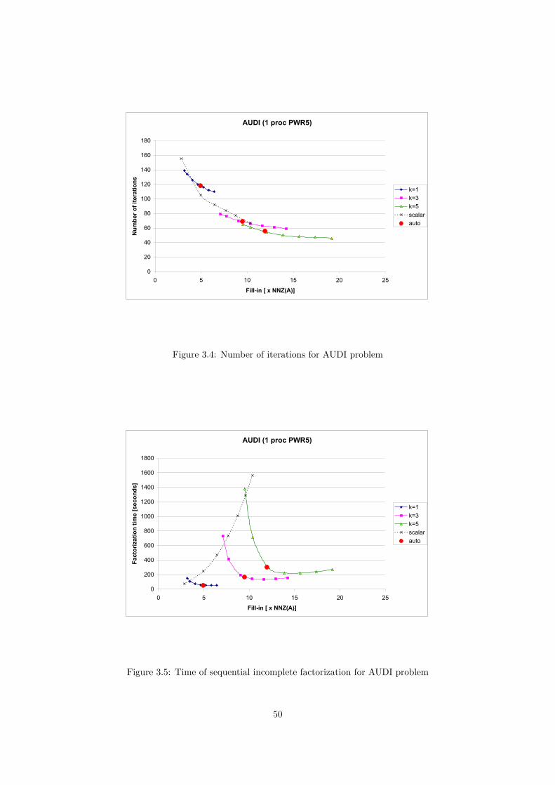
Figure 3.4: Number of iterations for AUDI problem

������������� ��

�

���

���

���

���

����

����

����

����

����

� � �� �� �� ��

�������������������

�������������������� ��

���

��

���

�� ��

����

Figure 3.5: Time of sequential incomplete factorization for AUDI problem

50

������������� ��

�

�

�

�

�

��

��

��

��

� � �� �� �� ��

�������������������

�������������� ��

���

��

���

�� ��

����

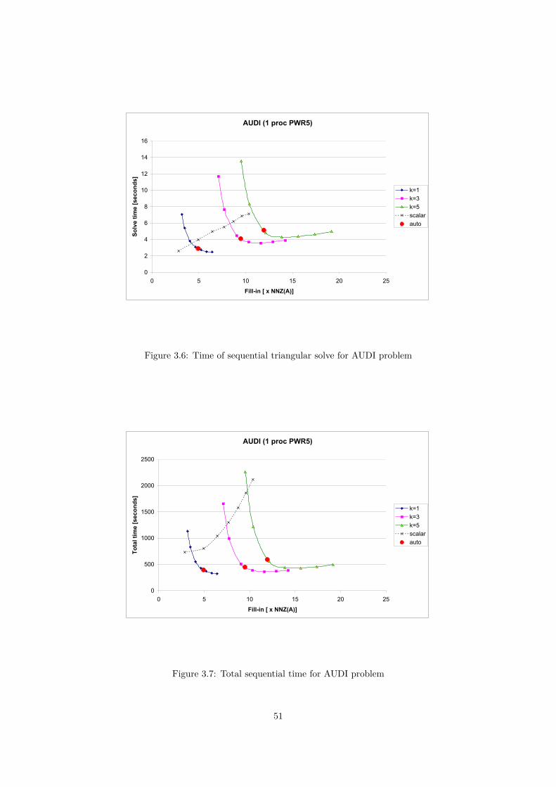
Figure 3.6: Time of sequential triangular solve for AUDI problem

������������� ��

�

���

����

����

����

����

� � �� �� �� ��

�������������������

�������������� ��

���

���

���

���

� �

Figure 3.7: Total sequential time for AUDI problem

51

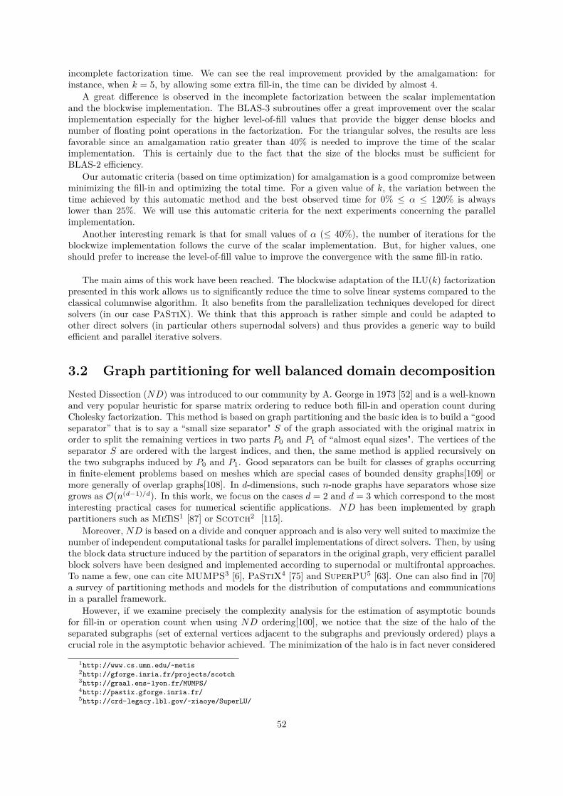
incomplete factorization time. We can see the real improvement provided by the amalgamation: forinstance, when k = 5, by allowing some extra fill-in, the time can be divided by almost 4.

A great difference is observed in the incomplete factorization between the scalar implementationand the blockwise implementation. The BLAS-3 subroutines offer a great improvement over the scalarimplementation especially for the higher level-of-fill values that provide the bigger dense blocks andnumber of floating point operations in the factorization. For the triangular solves, the results are lessfavorable since an amalgamation ratio greater than 40% is needed to improve the time of the scalarimplementation. This is certainly due to the fact that the size of the blocks must be sufficient forBLAS-2 efficiency.

Our automatic criteria (based on time optimization) for amalgamation is a good compromize betweenminimizing the fill-in and optimizing the total time. For a given value of k, the variation between thetime achieved by this automatic method and the best observed time for 0% ≤ α ≤ 120% is alwayslower than 25%. We will use this automatic criteria for the next experiments concerning the parallelimplementation.

Another interesting remark is that for small values of α (≤ 40%), the number of iterations for theblockwize implementation follows the curve of the scalar implementation. But, for higher values, oneshould prefer to increase the level-of-fill value to improve the convergence with the same fill-in ratio.

The main aims of this work have been reached. The blockwise adaptation of the ILU(k) factorizationpresented in this work allows us to significantly reduce the time to solve linear systems compared to theclassical columnwise algorithm. It also benefits from the parallelization techniques developed for directsolvers (in our case PaStiX). We think that this approach is rather simple and could be adapted toother direct solvers (in particular others supernodal solvers) and thus provides a generic way to buildefficient and parallel iterative solvers.

3.2 Graph partitioning for well balanced domain decompositionNested Dissection (ND) was introduced to our community by A. George in 1973 [52] and is a well-knownand very popular heuristic for sparse matrix ordering to reduce both fill-in and operation count duringCholesky factorization. This method is based on graph partitioning and the basic idea is to build a “goodseparator” that is to say a “small size separator" S of the graph associated with the original matrix inorder to split the remaining vertices in two parts P0 and P1 of “almost equal sizes". The vertices of theseparator S are ordered with the largest indices, and then, the same method is applied recursively onthe two subgraphs induced by P0 and P1. Good separators can be built for classes of graphs occurringin finite-element problems based on meshes which are special cases of bounded density graphs[109] ormore generally of overlap graphs[108]. In d-dimensions, such n-node graphs have separators whose sizegrows as O(n(d−1)/d). In this work, we focus on the cases d = 2 and d = 3 which correspond to the mostinteresting practical cases for numerical scientific applications. ND has been implemented by graphpartitioners such as MeTiS1 [87] or Scotch2 [115].

Moreover, ND is based on a divide and conquer approach and is also very well suited to maximize thenumber of independent computational tasks for parallel implementations of direct solvers. Then, by usingthe block data structure induced by the partition of separators in the original graph, very efficient parallelblock solvers have been designed and implemented according to supernodal or multifrontal approaches.To name a few, one can cite MUMPS3 [6], PaStiX4 [75] and SuperPU5 [63]. One can also find in [70]a survey of partitioning methods and models for the distribution of computations and communicationsin a parallel framework.

However, if we examine precisely the complexity analysis for the estimation of asymptotic boundsfor fill-in or operation count when using ND ordering[100], we notice that the size of the halo of theseparated subgraphs (set of external vertices adjacent to the subgraphs and previously ordered) plays acrucial role in the asymptotic behavior achieved. The minimization of the halo is in fact never considered

1http://www.cs.umn.edu/~metis2http://gforge.inria.fr/projects/scotch3http://graal.ens-lyon.fr/MUMPS/4http://pastix.gforge.inria.fr/5http://crd-legacy.lbl.gov/~xiaoye/SuperLU/

52

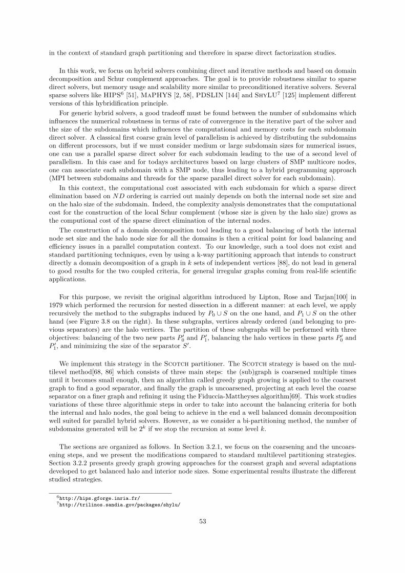
in the context of standard graph partitioning and therefore in sparse direct factorization studies.

In this work, we focus on hybrid solvers combining direct and iterative methods and based on domaindecomposition and Schur complement approaches. The goal is to provide robustness similar to sparsedirect solvers, but memory usage and scalability more similar to preconditioned iterative solvers. Severalsparse solvers like HIPS6 [51], MaPHYS [2, 58], PDSLIN [144] and ShyLU7 [125] implement differentversions of this hybridification principle.

For generic hybrid solvers, a good tradeoff must be found between the number of subdomains whichinfluences the numerical robustness in terms of rate of convergence in the iterative part of the solver andthe size of the subdomains which influences the computational and memory costs for each subdomaindirect solver. A classical first coarse grain level of parallelism is achieved by distributing the subdomainson different processors, but if we must consider medium or large subdomain sizes for numerical issues,one can use a parallel sparse direct solver for each subdomain leading to the use of a second level ofparallelism. In this case and for todays architectures based on large clusters of SMP multicore nodes,one can associate each subdomain with a SMP node, thus leading to a hybrid programming approach(MPI between subdomains and threads for the sparse parallel direct solver for each subdomain).

In this context, the computational cost associated with each subdomain for which a sparse directelimination based on ND ordering is carried out mainly depends on both the internal node set size andon the halo size of the subdomain. Indeed, the complexity analysis demonstrates that the computationalcost for the construction of the local Schur complement (whose size is given by the halo size) grows asthe computional cost of the sparse direct elimination of the internal nodes.

The construction of a domain decomposition tool leading to a good balancing of both the internalnode set size and the halo node size for all the domains is then a critical point for load balancing andefficiency issues in a parallel computation context. To our knowledge, such a tool does not exist andstandard partitioning techniques, even by using a k-way partitioning approach that intends to constructdirectly a domain decomposition of a graph in k sets of independent vertices [88], do not lead in generalto good results for the two coupled criteria, for general irregular graphs coming from real-life scientificapplications.

For this purpose, we revisit the original algorithm introduced by Lipton, Rose and Tarjan[100] in1979 which performed the recursion for nested dissection in a different manner: at each level, we applyrecursively the method to the subgraphs induced by P0 ∪ S on the one hand, and P1 ∪ S on the otherhand (see Figure 3.8 on the right). In these subgraphs, vertices already ordered (and belonging to pre-vious separators) are the halo vertices. The partition of these subgraphs will be performed with threeobjectives: balancing of the two new parts P ′0 and P ′1, balancing the halo vertices in these parts P ′0 andP ′1, and minimizing the size of the separator S′.

We implement this strategy in the Scotch partitioner. The Scotch strategy is based on the mul-tilevel method[68, 86] which consists of three main steps: the (sub)graph is coarsened multiple timesuntil it becomes small enough, then an algorithm called greedy graph growing is applied to the coarsestgraph to find a good separator, and finally the graph is uncoarsened, projecting at each level the coarseseparator on a finer graph and refining it using the Fiduccia-Mattheyses algorithm[69]. This work studiesvariations of these three algorithmic steps in order to take into account the balancing criteria for boththe internal and halo nodes, the goal being to achieve in the end a well balanced domain decompositionwell suited for parallel hybrid solvers. However, as we consider a bi-partitioning method, the number ofsubdomains generated will be 2k if we stop the recursion at some level k.

The sections are organized as follows. In Section 3.2.1, we focus on the coarsening and the uncoars-ening steps, and we present the modifications compared to standard multilevel partitioning strategies.Section 3.2.2 presents greedy graph growing approaches for the coarsest graph and several adaptationsdeveloped to get balanced halo and interior node sizes. Some experimental results illustrate the differentstudied strategies.

6http://hips.gforge.inria.fr/7http://trilinos.sandia.gov/packages/shylu/

53

������

������

���

���

��������

���

���

����

���

���

��������

������

������

������

������

����������

����������

������������

������������

������������������������

������������������������

�����

�����

���

���

������

������

���

���

Y = A u C u B

Classical Nested Dissection on A and B

(Alan George)Generalized Nested Dissection on A u C and B u C

(Lipton, Rose, Tarjan)

Figure 3.8: On the left: classical recursion which is performed on P0 and P1. Objectives are to balancethe sizes of the subgraphs and to minimize the separator size. However, halo sizes, represented by thenodes in black and grey, can be unbalanced: they are respectively 4, 5, 6 and 8. On the right: recursionis performed here on P0 ∪ S and P1 ∪ S and the halo vertices are balanced among the parts, leading tointerface sizes equal to 5, 5, 6 and 6.

54

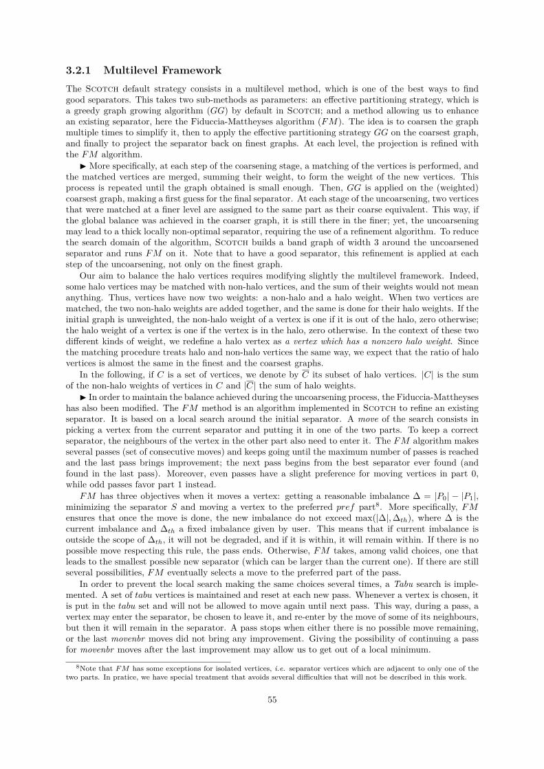
3.2.1 Multilevel FrameworkThe Scotch default strategy consists in a multilevel method, which is one of the best ways to findgood separators. This takes two sub-methods as parameters: an effective partitioning strategy, which isa greedy graph growing algorithm (GG) by default in Scotch; and a method allowing us to enhancean existing separator, here the Fiduccia-Mattheyses algorithm (FM). The idea is to coarsen the graphmultiple times to simplify it, then to apply the effective partitioning strategy GG on the coarsest graph,and finally to project the separator back on finest graphs. At each level, the projection is refined withthe FM algorithm.

I More specifically, at each step of the coarsening stage, a matching of the vertices is performed, andthe matched vertices are merged, summing their weight, to form the weight of the new vertices. Thisprocess is repeated until the graph obtained is small enough. Then, GG is applied on the (weighted)coarsest graph, making a first guess for the final separator. At each stage of the uncoarsening, two verticesthat were matched at a finer level are assigned to the same part as their coarse equivalent. This way, ifthe global balance was achieved in the coarser graph, it is still there in the finer; yet, the uncoarseningmay lead to a thick locally non-optimal separator, requiring the use of a refinement algorithm. To reducethe search domain of the algorithm, Scotch builds a band graph of width 3 around the uncoarsenedseparator and runs FM on it. Note that to have a good separator, this refinement is applied at eachstep of the uncoarsening, not only on the finest graph.

Our aim to balance the halo vertices requires modifying slightly the multilevel framework. Indeed,some halo vertices may be matched with non-halo vertices, and the sum of their weights would not meananything. Thus, vertices have now two weights: a non-halo and a halo weight. When two vertices arematched, the two non-halo weights are added together, and the same is done for their halo weights. If theinitial graph is unweighted, the non-halo weight of a vertex is one if it is out of the halo, zero otherwise;the halo weight of a vertex is one if the vertex is in the halo, zero otherwise. In the context of these twodifferent kinds of weight, we redefine a halo vertex as a vertex which has a nonzero halo weight. Sincethe matching procedure treats halo and non-halo vertices the same way, we expect that the ratio of halovertices is almost the same in the finest and the coarsest graphs.

In the following, if C is a set of vertices, we denote by C its subset of halo vertices. |C| is the sumof the non-halo weights of vertices in C and |C| the sum of halo weights.

I In order to maintain the balance achieved during the uncoarsening process, the Fiduccia-Mattheyseshas also been modified. The FM method is an algorithm implemented in Scotch to refine an existingseparator. It is based on a local search around the initial separator. A move of the search consists inpicking a vertex from the current separator and putting it in one of the two parts. To keep a correctseparator, the neighbours of the vertex in the other part also need to enter it. The FM algorithm makesseveral passes (set of consecutive moves) and keeps going until the maximum number of passes is reachedand the last pass brings improvement; the next pass begins from the best separator ever found (andfound in the last pass). Moreover, even passes have a slight preference for moving vertices in part 0,while odd passes favor part 1 instead.

FM has three objectives when it moves a vertex: getting a reasonable imbalance ∆ = |P0| − |P1|,minimizing the separator S and moving a vertex to the preferred pref part8. More specifically, FMensures that once the move is done, the new imbalance do not exceed max(|∆|,∆th), where ∆ is thecurrent imbalance and ∆th a fixed imbalance given by user. This means that if current imbalance isoutside the scope of ∆th, it will not be degraded, and if it is within, it will remain within. If there is nopossible move respecting this rule, the pass ends. Otherwise, FM takes, among valid choices, one thatleads to the smallest possible new separator (which can be larger than the current one). If there are stillseveral possibilities, FM eventually selects a move to the preferred part of the pass.

In order to prevent the local search making the same choices several times, a Tabu search is imple-mented. A set of tabu vertices is maintained and reset at each new pass. Whenever a vertex is chosen, itis put in the tabu set and will not be allowed to move again until next pass. This way, during a pass, avertex may enter the separator, be chosen to leave it, and re-enter by the move of some of its neighbours,but then it will remain in the separator. A pass stops when either there is no possible move remaining,or the last movenbr moves did not bring any improvement. Giving the possibility of continuing a passfor movenbr moves after the last improvement may allow us to get out of a local minimum.

8Note that F M has some exceptions for isolated vertices, i.e. separator vertices which are adjacent to only one of thetwo parts. In pratice, we have special treatment that avoids several difficulties that will not be described in this work.

55

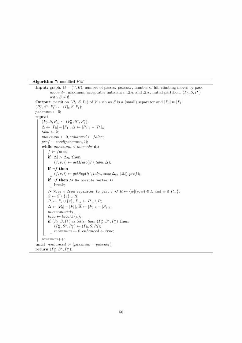
Algorithm 7: modified FMInput: graph: G = (V,E), number of passes: passnbr, number of hill-climbing moves by pass:

movenbr, maximum acceptable imbalance: ∆th and ∆th, initial partition: (P0, S, P1)with S 6= ∅

Output: partition (P0, S, P1) of V such as S is a (small) separator and |P0| ≈ |P1|(P ∗0 , S∗, P ∗1 )← (P0, S, P1);passnum← 0;repeat

(P0, S, P1)← (P ∗0 , S∗, P ∗1 );∆← |P0| − |P1|, ∆← |P0|h − |P1|h;tabu← ∅;movenum← 0, enhanced← false;pref ← mod(passnum, 2);while movenum < movenbr do

f ← false;if |∆| > ∆th then

(f, v, i)← getHalo(S \ tabu,∆);if ¬f then

(f, v, i)← getSep(S \ tabu,max(∆th, |∆|), pref);if ¬f then /* No movable vertex */

break;/* Move v from separator to part i */ R← {w|(v, w) ∈ E and w ∈ P¬i};S ← S \ {v} ∪R;Pi ← Pi ∪ {v}, P¬i ← P¬i \R;∆← |P0| − |P1|, ∆← |P0|h − |P1|h;movenum++;tabu← tabu ∪ {v};if (P0, S, P1) is better than (P ∗0 , S∗, P ∗1 ) then

(P ∗0 , S∗, P ∗1 )← (P0, S, P1);movenum← 0, enhanced← true;

passnum++;until ¬enhanced or (passnum = passnbr);return (P ∗0 , S∗, P ∗1 );

56

Our modified FM algorithm is presented in Algorithm 7. The choice of a vertex v to move from theseparator to a part i is revisited. If the current partition does not have an absolute halo imbalance |∆|below the threshold ∆th (chosen by user), then the function getHalo is called line 7. This function triesto fix the halo imbalance. It uses the sign of ∆ = |P0|h− |P1|h to know the part where a vertex must bemoved: a move to part 0 increases ∆, a move to part 1 decreases it. Then, it picks a vertex whose moveto part i will minimize the new halo imbalance. If there is no such move that improves ∆ strictly, thenthe function fails. Here, or if the partition had already a reasonable halo imbalance, the function getSepis called instead (line 7), which works as described in the unmodified version.

We conclude this section by giving our strategy to choose the better partition as indicated at line 7of Algorithm 7. We proceed as follows:

• if we never found a partition in which |∆| ≤ ∆th, we keep the partition whose |∆| is the smallest.

• if we already found a partition satisfying |∆| ≤ ∆th, but never a partition satisfying both |∆| ≤ ∆th

and |∆| ≤ ∆th, then we keep a partition with |∆| ≤ ∆th whose |∆| is the smallest.

• if we already found a partition satisfying both |∆| ≤ ∆th and |∆| ≤ ∆th, we keep only partitionssatisfying these two conditions; among them, we choose the one which has the smallest separator.In case of equality, we pick the one with the smallest |∆|, and if there is still a tie, the one withthe smallest |∆|.

3.2.2 Graph Partitioning AlgorithmsWe also need to adapt the greedy graph growing (GG) algorithm in order to compute a partitioning whichtakes halo weight into account. The next subsection will present the GG algorithm and a straightforwardadaptation. Some unsatisfactory results lead us to consider two other approaches that are presented inthe last two subsections and named double GG and halo-first GG respectively. The first one shares theidea of the "bubble" algorithm of [45, 107] to do GG with one seed per part, although it is based on adifferent approach.

Table 3.1 presents all the testing matrices, giving their size and their number of nonzero entries. Theid number will be used to identify matrices in the following. For each matrix A, the symmetric graphof A+At is used. Matrices 1-20 come from the University of Florida Sparse Matrix Collection, and thelast set of ten matrices comes from PARASOL collection, industrial collaborations or partners.

Algorithms will be judged on two criteria. For each domain, the sizes of the interior and of thehalo are measured. Then, we compute the difference between the maximum and the minium for both,providing two metrics: interface imbalance, and interior imbalance. For example, on the bottom-rightgraph in Figure 3.8, interior sizes are all equal to 4, thus the interior imbalance is null, and halo sizesare 5, 5, 6, and 6 respectively, giving a halo imbalance equal to 1.

Note that the graph partitioning technique used for ND is designed for reordering purpose. In thiscontext, the main objective of Scotch software is to minimize the size of the separator while keeping alocal imbalance for interior sizes that does not exceed a fixed percentage, named bal. The recursion isperformed until a fixed number of vertices is reached. Thus, the branches of the decomposition tree mayhave different heights. On the contrary, we focus in this work on decomposition domain : so we want tochoose the number of domains and thus the number of levels in the recursion. Furthermore, a defaultvalue for the local constraint on the interior imbalance (bal = 10%) accumulates through levels of therecursion: at level i, imbalance between minimum and maximum subgraph sizes may reach roughly bal×ipercents. This is too loose for our purpose. We cannot decrease bal too much because the constraintwould be too tight for having a chance to minimize the separator. Thus, to achieve good balancing,we use a constraint that depends on the level: on the higher levels, subgraphs are big, so we can usea tighter constraint while giving the possibility of optimizing the separator size; on the bottom levels,subgraphs are small and we use a looser constraint. More precisely, if p levels are requested, level i willtry to get a local imbalance of at most max( bal

2p−i+1 ,minbal), where minbal is a threshold ensuring thatthe constraint does not become too small.

57

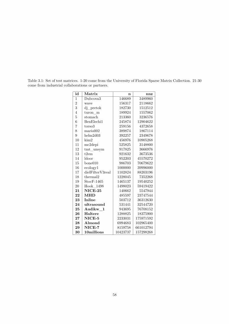
Table 3.1: Set of test matrices. 1-20 come from the University of Florida Sparse Matrix Collection. 21-30come from industrial collaborations or partners.

id Matrix n nnz1 Dubcova3 146689 34899602 wave 156317 21186623 dj_pretok 182730 15125124 turon_m 189924 15570625 stomach 213360 32365766 BenElechi1 245874 129046227 torso3 259156 43726588 mario002 389874 18671149 helm2d03 392257 234967810 kim2 456976 1090526811 mc2depi 525825 314880012 tmt_unsym 917825 366697613 t2em 921632 367353614 ldoor 952203 4557027215 bone010 986703 7067962216 ecology1 1000000 3999600017 dielFilterV3real 1102824 8820319618 thermal2 1228045 735226819 StocF-1465 1465137 1954025220 Hook_1498 1498023 5941942221 NICE-25 140662 554794422 MHD 485597 2374754423 Inline 503712 3631263024 ultrasound 531441 3254472025 Audikw_1 943695 7670815226 Haltere 1288825 1837590027 NICE-5 2233031 17597159228 Almond 6994683 10296540029 NICE-7 8159758 66101279430 10millions 10423737 157298268

58

In the following, all tests are done with a fixed number of levels of recursion. The column GG(standing for Greedy Graph Growing) in the results refers to the unmodified Scotch strategy, withbal = 10%. The column GG? and the other columns use the level-dependent constraint described abovewith bal = 10% and a threshold of 1%. GG? thus refers to a modified Scotch strategy with defaultgraph partitioning algorithms but using the level-dependent bal constraint.

Greedy Graph Growing

The algorithm implemented by the Scotch software to find a good separator in a graph G = (V,E)at the bottom of the multilevel technique is the greedy graph growing method. The idea is to pick arandom seed vertex in the graph, and to make a part grow from this seed, until it reaches half of thegraph size. It is described in Algorithm 8. At line 8, the seed w is chosen. Singleton {w} is the initialseparator S between the parts P1, empty, and P0, containing all other vertices. Then, at each step, avertex v from current separator S is chosen (l. 8), and passed from the separator S to the growing partP1 (l. 8 and 8). The choice is oriented by the minimization of the current separator. Additionally, theset N of all neighbours of v in P0 are retrieved from P0 (l. 8) and added to S (l. 8), so that S remains aseparator for the parts. The process is repeated until both parts have almost the same size.

The result of this algorithm is very dependent on the random seed chosen at the beginning. Thus,Scotch tries several passes with different seeds (l. 8), and it eventually selects the best partition(P0, S, P1) found in all passes (l. 8).

Algorithm 8: GreedyGraphGrowingInput: graph G = (V,E), number of passes passnbrOutput: partition (P0, S, P1) of V such as S is a (small) separator and |P0| ≈ |P1|(P ∗0 , S∗, P ∗1 )← (∅, V, ∅);for p = 1 to passnbr do

w ← RandomSeed(V ) ;P0 ← V \ {w};P1 ← ∅;S ← {w};while |P0| and |P1| are not balanced do

v ← getV ertex(S) ;N ← {j|(v, j) ∈ E and j ∈ P0} ; /* neighbours of v in P0 */S ← S \ {v} ∪N ;P0 ← P0 \N ;P1 ← P1 ∪ {v};

if (P0, S, P1) is better than (P ∗0 , S∗, P ∗1 ) then(P ∗0 , S∗, P ∗1 )← (P0, S, P1);

return (P ∗0 , S∗, P ∗1 );

In a first attempt to adapt this algorithm to our purpose of balancing the halo, we made the followingchanges. First, the choice of the vertex to move from S to P1 was now oriented by the halo balance.More specifically, if P1 had not as many halo vertices as P0 (relative to the respective size of the parts),then we preferably chooses a vertex v inside the halo. Secondly, note that it is needed to have boththe halo and the non-halo vertices in the separator for this strategy to work well. We thus choose therandom seed inside halo, since halo vertices are often close to each other.

We tested this adapted algorithm. Unfortunately, if often fails to improve the default partitioningstrategy.

Double Greedy Graph Growing with Halo Care

The previous algorithm managed a good halo balance in general, but often at the price of a disconnectedpart P0. We thus decided to use two initial seeds, one for each part, and to make both parts growsimultaneously. However, this new strategy can lead to blocking. Indeed, when growing, one part mayblock the progression of the other: this happens when V \ (P0 ∪ P1) is not empty but has no vertex

59

reachable from some part Pi. To avoid this problem, we need to delay, as much as possible, the momentwhen parts meet each other.

Algorithm 9 describes the new method. Line 9 picks the two seeds wi and w¬i in the halo. They arealso chosen as far as possible from each other, so that parts meet as late as possible. Both parts, initiallyempty, are grown from their respective seed vertex. At each step, we choose the smallest part i (l. 9-9),and a vertex v from its boundary Si (l. 9). v is chosen according to the halo balance situation; if part i hasless halo vertices than part ¬i, a halo vertex is taken if possible, and if it has more halo vertices, a non-halo vertex is picked preferably. If several choices of vertices remain, then the vertex which is the nearestfrom wi and the farthest from w¬i (i.e. the vertex v with the smallest value dist(v, wi) − dist(v, w¬i))is taken. This is still with the purpose of making the parts meet as late as possible. Like the single-seedgreedy graph growing presented before, v is then added to Pi (l. 9), retrieved from Si, and Si is updatedto remain the boundary of Pi (l. 9). The process is carried on until all vertices are in one of the twoparts, meaning V \ (P0 ∪ P1) = ∅ (end of while loop l. 9), or we are blocked, namely Si = ∅ (l. 9).

In the latter case, a solution would be to put all remaining vertices of V \(P0∪P1) in the part to whichthey are adjacent. If few vertices remain, this is actually the solution we take lines 9-9. Otherwise, weempty P0 and P1 (l. 9) and retry to grow the parts from w0 and w1, using some additional information toavoid getting blocked again. More specifically, we define a set of control points for each part i, containingonly their respective seed at the beginning. When blocked, we add a new control point to the part i whichcould not grow. This control point is defined by the vertex of Pi which is the nearest from the untakenvertices. Then, parts are made grown again. When we choose a vertex to add to part i (l. 9), the firstcriterion is still the halo situation, and the second criterion is now the vertex v with the smallest valueminj{dist(v, ctrlptsi[j])}−minj{dist(v, ctrlpts¬i[j])}. In other words, part i will be attracted by its owncontrol points, and repulsed by the control points of ¬i. (Note that this rule is in fact a generalizationof the previous one).

The strategy described before is repeated until we either succeed to construct a partition (P0, P1)of V from (w0, w1), or we reach triesnb tries, meaning we failed. If we succeed, we can construct aseparator S by applying a minimum vertex cover algorithm on the edges on the frontier of P0 and P1(l. 9).

Like in the previous algorithm, several passes are made with different couples of seed vertices. Weeventually select the best partition found among the successful passes on line 9.

We tested double greedy graph growing on 4 levels of recursion (i.e. 16 domains). The results arepresented in Table 3.2. The columns GG give the interface and interior imbalance of unmodified Scotchwith bal = 10%. Other columns only give a percentage relative to the corresponding GG column. For ex-ample, for the matrix ecology1 (16), double greedy graph growing (denoted by the DG column) achievesa halo imbalance 62, 9% better than unmodified GG, that is a halo imbalance of (1−0.629)×564 ' 209.The column GG? refers to a modified Scotch with a balance depending on the level (see introductionof this section). For each criterion, we highlighted in bold the best result.

We can see that interface balancing of DG is much better than unmodified GG and GG? for all buttwo matrices. The gain can be up to 78, 5% on matrix MHD (22), with an average of 40% over all matrices.DG also achieves a better interior balancing in general compared to GG, on all but two matrices; theaverage gain for this column is 45%. It is also better than GG? on one third of the test cases, which israther good since it has one more criterion to optimize. Moreover, we can see that on all but one of theindustrial matrices (which are of particular interest for us), gains are very good on both criteria.

Halo-first Greedy Graph Growing

In the previous section, we have studied an algorithm that constructs a separator for the parts and forthe halo at once. This gives priority to minimizing the separator, while trying to balance the halo whenpossible. In this section, we review another approach, which consists in finding a halo separator first.Once this is done, we construct a separator for the whole graph, making the parts grow from the partsinduced by this halo separator.

Before splitting the graph of the halo, we first have to build the graph. We could take the graph(Vh = V ,Eh = E ∩ (Vh × Vh)), defined by the restriction of the whole graph to the halo vertices and theedges connecting them. Nevertheless, this graph may not be connected, even if the whole graph is. Inthe worst case, it can be totally disconnected, and considering the far-away neighbourhood may not be

60

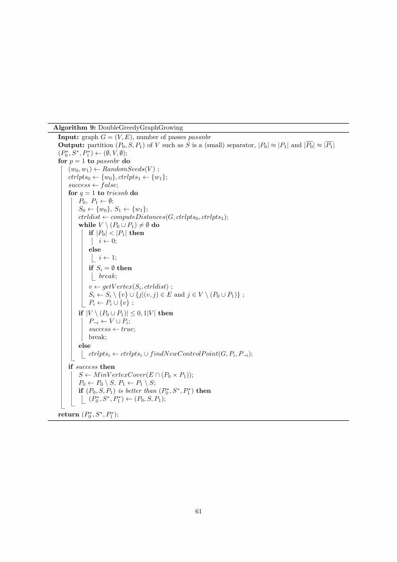
Algorithm 9: DoubleGreedyGraphGrowingInput: graph G = (V,E), number of passes passnbrOutput: partition (P0, S, P1) of V such as S is a (small) separator, |P0| ≈ |P1| and |P0| ≈ |P1|(P ∗0 , S∗, P ∗1 )← (∅, V, ∅);for p = 1 to passnbr do

(w0, w1)← RandomSeeds(V ) ;ctrlpts0 ← {w0}, ctrlpts1 ← {w1};success← false;for q = 1 to triesnb do

P0, P1 ← ∅;S0 ← {w0}, S1 ← {w1};ctrldist← computeDistances(G, ctrlpts0, ctrlpts1);while V \ (P0 ∪ P1) 6= ∅ do

if |P0| < |P1| theni← 0;

elsei← 1;

if Si = ∅ thenbreak;

v ← getV ertex(Si, ctrldist) ;Si ← Si \ {v} ∪ {j|(v, j) ∈ E and j ∈ V \ (P0 ∪ P1)} ;Pi ← Pi ∪ {v} ;

if |V \ (P0 ∪ P1)| ≤ 0, 1|V | thenP¬i ← V ∪ Pi;success← true;break;

elsectrlptsi ← ctrlptsi ∪ findNewControlPoint(G,Pi, P¬i);

if success thenS ←MinV ertexCover(E ∩ (P0 × P1));P0 ← P0 \ S, P1 ← P1 \ S;if (P0, S, P1) is better than (P ∗0 , S∗, P ∗1 ) then

(P ∗0 , S∗, P ∗1 )← (P0, S, P1);

return (P ∗0 , S∗, P ∗1 );

61

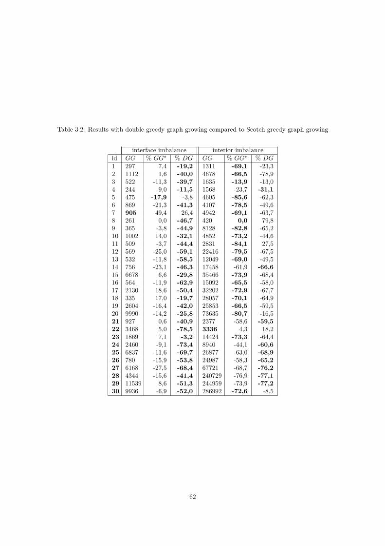
Table 3.2: Results with double greedy graph growing compared to Scotch greedy graph growing

interface imbalance interior imbalanceid GG % GG? % DG GG % GG? % DG1 297 7,4 -19,2 1311 -69,1 -23,32 1112 1,6 -40,0 4678 -66,5 -78,93 522 -11,3 -39,7 1635 -13,9 -13,04 244 -9,0 -11,5 1568 -23,7 -31,15 475 -17,9 -3,8 4605 -85,6 -62,36 869 -21,3 -41,3 4107 -78,5 -49,67 905 49,4 26,4 4942 -69,1 -63,78 261 0,0 -46,7 420 0,0 79,89 365 -3,8 -44,9 8128 -82,8 -65,210 1002 14,0 -32,1 4852 -73,2 -44,611 509 -3,7 -44,4 2831 -84,1 27,512 569 -25,0 -59,1 22416 -79,5 -67,513 532 -11,8 -58,5 12049 -69,0 -49,514 756 -23,1 -46,3 17458 -61,9 -66,615 6678 6,6 -29,8 35466 -73,9 -68,416 564 -11,9 -62,9 15092 -65,5 -58,017 2130 18,6 -50,4 32202 -72,9 -67,718 335 17,0 -19,7 28057 -70,1 -64,919 2604 -16,4 -42,0 25853 -66,5 -59,520 9990 -14,2 -25,8 73635 -80,7 -16,521 927 0,6 -40,9 2377 -58,6 -59,522 3468 5,0 -78,5 3336 4,3 18,223 1869 7,1 -3,2 14424 -73,3 -64,424 2460 -9,1 -73,4 8940 -44,1 -60,625 6837 -11,6 -69,7 26877 -63,0 -68,926 780 -15,9 -53,8 24987 -58,3 -65,227 6168 -27,5 -68,4 67721 -68,7 -76,228 4344 -15,6 -41,4 240729 -76,9 -77,129 11539 8,6 -51,3 244959 -73,9 -77,230 9936 -6,9 -52,0 286992 -72,6 -8,5

62

enough to reconnect it. However, it is important to take graph connections into account because choosingwhich of the halo vertices will be in each part at random would often lead to a very poor separator ofthe whole graph.

To deal with this issue, we use the following algorithm to build a graph containing all relevant infor-mation about the halo vertices. A partition of the halo vertices is maintained. At the beginning, eachhalo vertex is in a different set of the partition, and a set V ′h is initialized with all halo vertices. Then,we make simultaneous breadth-first searches from all the sets of the partition. When two search bubblescorresponding to different sets meet, this means a shortest-path between any two sets of the partitionhas been found. All vertices of this path are added to V ′h. The sets which have met are merged, and thebreadth-first-search is continued. The process stops when either all sets of the partition have merged -meaning the graph is connected -, or all breadth-first searches have finished. Finally, the graph of thehalo is defined by (V ′h, E′h = E ∩ (V ′h×V ′h)). Ignoring the time for partition managing operations (whichis almost constant), the complexity to build the halo graph is equivalent to a single global breadth-firstsearch, that is Θ(|V |+ |E|).

Now, let buildConnectedHalo be a function building such a graph (V ′h, E′h). Algorithm 10 gives themain steps to find a separator. A first greedy graph growing algorithm is performed to compute a cut ofthe halo (V ′h0, S

′h, V

′h1). Next, a kind of double greedy graph growing is done, beginning with the set of

seed V ′h0 for part 0, and V ′h1 for part 1. Finally, we get a partition (P0, S, P1). As in the other algorithms,these steps can be repeated, doing several passes and keeping the best one.

Algorithm 10: HaloFirstGreedyGraphGrowingInput: graph G = (V,E), number of passes passnbrOutput: partition (P0, S, P1) of V such as S is a (small) separator, |P0| ≈ |P1| and |P0| ≈ |P1|(P ∗0 , S∗, P ∗1 )← (∅, V, ∅);(V ′h, E′h)← buildConnectedHalo(V,E, Vh);for p = 1 to passnbr do

(V ′h0, S′h, V

′h1)← greedyGraphGrowing(V ′h, E′h);

(P0, S, P1)← doubleGreedyGraphGrowing(V,E, V ′h0, V′h1);

if (P0, S, P1) is better than (P ∗0 , S∗, P ∗1 ) then(P ∗0 , S∗, P ∗1 )← (P0, S, P1);

return (P ∗0 , S∗, P ∗1 );

We have applied the same testing protocol as in the previous subsection 3.2.2. The results are shownin Table 3.3 where the column HF refers to the halo-first greedy graph growing algorithm. A sign hasbeen added to the right of each column of HF : a ’+’ means that this gain is better (i.e. smaller) thanthe corresponding DG gain and a ’−’ that DG is better.

On the interface criterion, the HF approach is better than unmodified GG and GG? in all but fourmatrices. The worst case is the turon_m (4), but this apparent failure is due to the fact that GG performsvery well on this matrix: the interface imbalance is only 244 for 189924 vertices. Globally, the averagegain of HF over unmodified GG on interface imbalance is 38%, with a maximum of 75, 4%; this is almostas good as DG. If we compare gains of HF over DG on this criteria, we have 16 ’+’ out of 30, whichconfirms this tendency.

Moreover, HF achieves gains on the interior imbalance in all but one matrix. On average, interiorimbalance gain of HF is 56%. This is about 10% better than DG, and if gains are compared one byone, HF beats DG on two thirds of the matrices. DG is not obsolete however: for instance, on matrixultrasound (24), DG performs better than HF on both criteria.

3.2.3 Experimental ResultsIn order to see what are the characteristics of GG, DG and HF , we drew the partitioning performedby these algorithms on 16 domains on a small mesh called darcy003, without the multilevel framework.Figure 3.9 gives the results obtained. It can be seen that GG makes domains with irregular shapes,

63

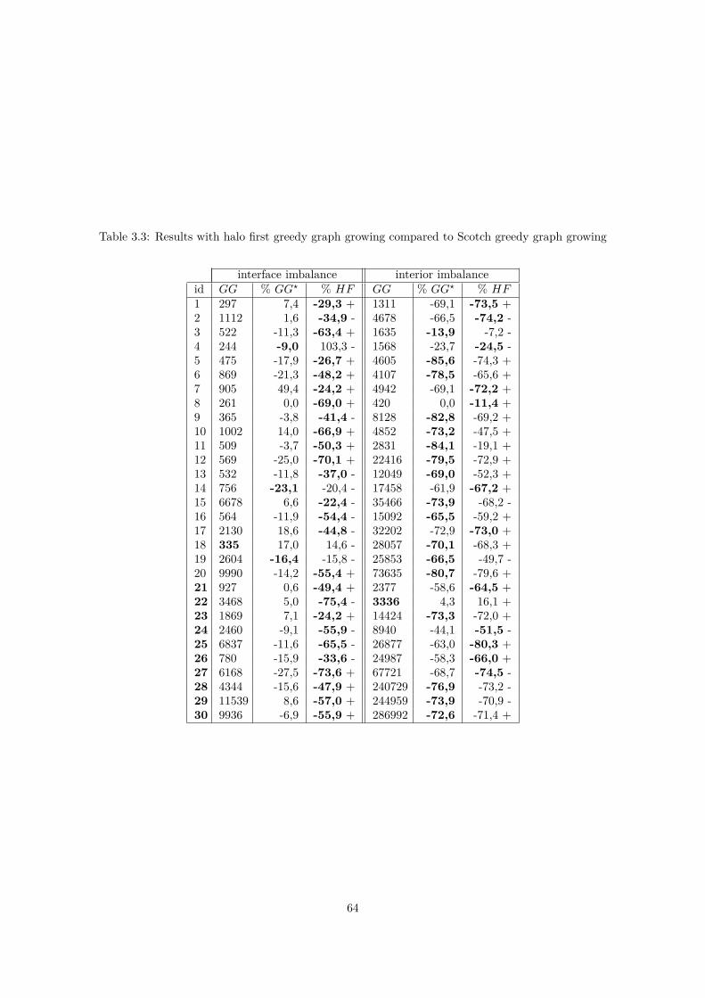
Table 3.3: Results with halo first greedy graph growing compared to Scotch greedy graph growing

interface imbalance interior imbalanceid GG % GG? % HF GG % GG? % HF1 297 7,4 -29,3 + 1311 -69,1 -73,5 +2 1112 1,6 -34,9 - 4678 -66,5 -74,2 -3 522 -11,3 -63,4 + 1635 -13,9 -7,2 -4 244 -9,0 103,3 - 1568 -23,7 -24,5 -5 475 -17,9 -26,7 + 4605 -85,6 -74,3 +6 869 -21,3 -48,2 + 4107 -78,5 -65,6 +7 905 49,4 -24,2 + 4942 -69,1 -72,2 +8 261 0,0 -69,0 + 420 0,0 -11,4 +9 365 -3,8 -41,4 - 8128 -82,8 -69,2 +10 1002 14,0 -66,9 + 4852 -73,2 -47,5 +11 509 -3,7 -50,3 + 2831 -84,1 -19,1 +12 569 -25,0 -70,1 + 22416 -79,5 -72,9 +13 532 -11,8 -37,0 - 12049 -69,0 -52,3 +14 756 -23,1 -20,4 - 17458 -61,9 -67,2 +15 6678 6,6 -22,4 - 35466 -73,9 -68,2 -16 564 -11,9 -54,4 - 15092 -65,5 -59,2 +17 2130 18,6 -44,8 - 32202 -72,9 -73,0 +18 335 17,0 14,6 - 28057 -70,1 -68,3 +19 2604 -16,4 -15,8 - 25853 -66,5 -49,7 -20 9990 -14,2 -55,4 + 73635 -80,7 -79,6 +21 927 0,6 -49,4 + 2377 -58,6 -64,5 +22 3468 5,0 -75,4 - 3336 4,3 16,1 +23 1869 7,1 -24,2 + 14424 -73,3 -72,0 +24 2460 -9,1 -55,9 - 8940 -44,1 -51,5 -25 6837 -11,6 -65,5 - 26877 -63,0 -80,3 +26 780 -15,9 -33,6 - 24987 -58,3 -66,0 +27 6168 -27,5 -73,6 + 67721 -68,7 -74,5 -28 4344 -15,6 -47,9 + 240729 -76,9 -73,2 -29 11539 8,6 -57,0 + 244959 -73,9 -70,9 -30 9936 -6,9 -55,9 + 286992 -72,6 -71,4 +

64

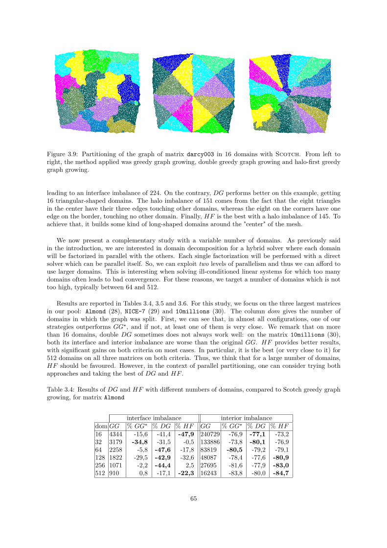
Figure 3.9: Partitioning of the graph of matrix darcy003 in 16 domains with Scotch. From left toright, the method applied was greedy graph growing, double greedy graph growing and halo-first greedygraph growing.

leading to an interface imbalance of 224. On the contrary, DG performs better on this example, getting16 triangular-shaped domains. The halo imbalance of 151 comes from the fact that the eight trianglesin the center have their three edges touching other domains, whereas the eight on the corners have oneedge on the border, touching no other domain. Finally, HF is the best with a halo imbalance of 145. Toachieve that, it builds some kind of long-shaped domains around the "center" of the mesh.

We now present a complementary study with a variable number of domains. As previously saidin the introduction, we are interested in domain decomposition for a hybrid solver where each domainwill be factorized in parallel with the others. Each single factorization will be performed with a directsolver which can be parallel itself. So, we can exploit two levels of parallelism and thus we can afford touse larger domains. This is interesting when solving ill-conditioned linear systems for which too manydomains often leads to bad convergence. For these reasons, we target a number of domains which is nottoo high, typically between 64 and 512.

Results are reported in Tables 3.4, 3.5 and 3.6. For this study, we focus on the three largest matricesin our pool: Almond (28), NICE-7 (29) and 10millions (30). The column dom gives the number ofdomains in which the graph was split. First, we can see that, in almost all configurations, one of ourstrategies outperforms GG?, and if not, at least one of them is very close. We remark that on morethan 16 domains, double DG sometimes does not always work well: on the matrix 10millions (30),both its interface and interior imbalance are worse than the original GG. HF provides better results,with significant gains on both criteria on most cases. In particular, it is the best (or very close to it) for512 domains on all three matrices on both criteria. Thus, we think that for a large number of domains,HF should be favoured. However, in the context of parallel partitioning, one can consider trying bothapproaches and taking the best of DG and HF .

Table 3.4: Results of DG and HF with different numbers of domains, compared to Scotch greedy graphgrowing, for matrix Almond

interface imbalance interior imbalancedom GG % GG? % DG % HF GG % GG? % DG % HF16 4344 -15,6 -41,4 -47,9 240729 -76,9 -77,1 -73,232 3179 -34,8 -31,5 -0,5 133886 -73,8 -80,1 -76,964 2258 -5,8 -47,6 -17,8 83819 -80,5 -79,2 -79,1128 1822 -29,5 -42,9 -32,6 48087 -78,4 -77,6 -80,9256 1071 -2,2 -44,4 2,5 27695 -81,6 -77,9 -83,0512 910 0,8 -17,1 -22,3 16243 -83,8 -80,0 -84,7

65

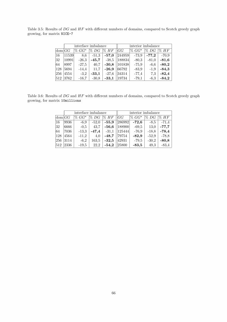
Table 3.5: Results of DG and HF with different numbers of domains, compared to Scotch greedy graphgrowing, for matrix NICE-7

interface imbalance interior imbalancedom GG % GG? % DG % HF GG % GG? % DG % HF16 11539 8,6 -51,3 -57,0 244959 -73,9 -77,2 -70,932 10991 -26,3 -45,7 -38,5 188834 -80,3 -81,0 -81,664 8997 -27,5 40,7 -30,8 101838 -75,9 -6,6 -80,2128 5694 -14,4 11,7 -26,9 66792 -83,9 -1,9 -84,3256 4554 -3,2 -33,1 -27,6 34314 -77,4 7,3 -82,4512 3762 -16,7 -30,8 -33,1 19734 -79,1 -6,3 -84,2

Table 3.6: Results of DG and HF with different numbers of domains, compared to Scotch greedy graphgrowing, for matrix 10millions

interface imbalance interior imbalancedom GG % GG? % DG % HF GG % GG? % DG % HF16 9936 -6,9 -52,0 -55,9 286992 -72,6 -8,5 -71,432 6666 -0,5 43,7 -56,6 188900 -69,5 13,0 -77,764 7036 -13,3 -47,4 -31,1 125444 -76,9 -18,8 -78,4128 4564 -11,2 4,0 -48,7 79754 -82,9 -52,9 -78,8256 3114 -6,2 163,5 -32,5 42931 -79,5 -30,2 -80,8512 2336 -19,5 22,2 -54,2 25800 -83,5 49,3 -83,4

66

Chapter 4

Towards H-matrices in sparse directsolvers

This chapter presents the work that is currently developed in the PhD thesis of Grégoire Pichon that Ico-advise. The first part of this chapter have been published in [120] and the second part in [119].

Please look at http://www.labri.fr/perso/ramet/restricted/HDR_SIMAX17.pdf and also at http://www.labri.fr/perso/ramet/restricted/HDR_PDSEC17.pdf for a full version of this work with someexperiments.

4.1 Reordering strategy for blocking optimizationThe block-symbolic factorization [38] analytically computes the block-structure of the factorized matrixfrom the reordering step and from a supernode partition of the unknowns. It allows the solver to createthe data structure that will hold the final matrix instead of allocating it at runtime. The goal of thisstep is also to block the data in order to efficiently apply matrix-matrix operations, also known as BLASLevel 3, on those blocks instead of scalar operations. For this purpose, extra fill-in, and by extent extracomputations, might be added in order to reduce the time to solution. However, the size of these blocksmight not be sufficiently large to obtain the full performance from the BLAS kernels.

Modern architectures, whether based on CPUs, GPUs, or Intel Xeon Phi may be efficient with aperformance close to the theoretical peak. This can be achieved only if the data size is large enough totake advantage of caches, vector units, and provides a large ratio of computation per byte. Acceleratorssuch as GPUs or Intel Xeon Phi require even larger blocking sizes than those for CPUs due to theirparticular architectural features.

In order to obtain block sizes more suited to kernel operations, we propose in this work an algorithmthat reorders the unknowns of the problem to increase the average size of the off-diagonal blocks in block-symbolic factorization structures. The major feature of this solution is that, based on an existing nesteddissection ordering for a given problem, our solution will keep constant the amount of fill-in generatedduring the factorization. Therefore, the amount of memory and computation to store and compute thefactorized matrix is invariant. The consequence of this increased average size is that the number ofoff-diagonal blocks is significantly reduced, diminishing the memory overhead of the data structures usedby the solver and the number of tasks required to compute the solution in task-based implementations.

4.1.1 Intra-node reorderingLet us now illustrate the problem of current ordering solutions and how to overcome this problem. Forthis purpose, we consider a regular 3D cube of n3 vertices presented in Figure 4.1. We apply the nesteddissection process to this cube. Naturally, the first separator, in gray, is a plane of n2 vertices cutting thecube into two halves of balanced parts. Then, by recursively applying the nested dissection process, wepartition the two-halves’ subparts with the two red separators, and again dissect the resulting partitionsby the four third-level green separators giving us eight final partitions. We know from this process thateach separator will be ordered with higher indices than those in lower levels.

67

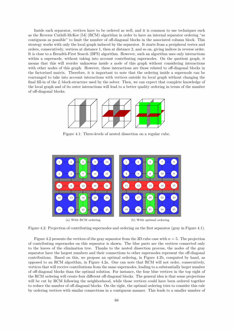
Inside each separator, vertices have to be ordered as well, and it is common to use techniques suchas the Reverse Cuthill-McKee [54] (RCM) algorithm in order to have an internal separator ordering “ascontiguous as possible” to limit the number of off-diagonal blocks in the associated column block. Thisstrategy works with only the local graph induced by the separator. It starts from a peripheral vertex andorders, consecutively, vertices at distance 1, then at distance 2, and so on, giving indices in reverse order.It is close to a Breadth-First Search (BFS) algorithm. However, such an algorithm uses only interactionswithin a supernode, without taking into account contributing supernodes. On the quotient graph, itmeans that this will reorder unknowns inside a node of this graph without considering interactionswith other nodes of this graph. However, these interactions are those related to off-diagonal blocks inthe factorized matrix. Therefore, it is important to note that the ordering inside a supernode can berearranged to take into account interactions with vertices outside its local graph without changing thefinal fill-in of the L block-structure used by the solver. Then, we can expect that complete knowledge ofthe local graph and of its outer interactions will lead to a better quality ordering in terms of the numberof off-diagonal blocks.

Figure 4.1: Three-levels of nested dissection on a regular cube.

1 2 5 9 14

3 4 7 11 17

6 8 12 16 21

10 13 18 20 23

15 19 22 24 25

1 2 5 9 14

3 4 7 11 17

6 8 12 16 21

10 13 18 20 23

15 19 22 24 25

(a) With RCM ordering

1 2 5 7 8

3 4 6 10 9

11 12 13 14 15

16 17 20 22 23

19 18 21 24 25

1 2 5 7 8

3 4 6 10 9

11 12 13 14 15

16 17 20 22 23

19 18 21 24 25

(b) With optimal ordering

Figure 4.2: Projection of contributing supernodes and ordering on the first separator (gray in Figure 4.1).

Figure 4.2 presents the vertices of the gray separator from the 3D cube case with n = 5. The projectionof contributing supernodes on this separator is shown. The blue parts are the vertices connected onlyto the leaves of the elimination tree. Thanks to the nested dissection process, the nodes of the grayseparator have the largest numbers and their connections to other supernodes represent the off-diagonalcontributions. Based on this, we propose an optimal ordering, in Figure 4.2b, computed by hand, asopposed to an RCM algorithm, in Figure 4.2a. One can note that RCM will not order, consecutively,vertices that will receive contributions from the same supernodes, leading to a substantially larger numberof off-diagonal blocks than the optimal solution. For instance, the four blue vertices in the top right ofthe RCM ordering will create four different off-diagonal blocks. The general idea is that some projectionswill be cut by RCM following the neighborhood, while those vertices could have been ordered togetherto reduce the number of off-diagonal blocks. On the right, the optimal ordering tries to consider this ruleby ordering vertices with similar connections in a contiguous manner. This leads to a smaller number of

68

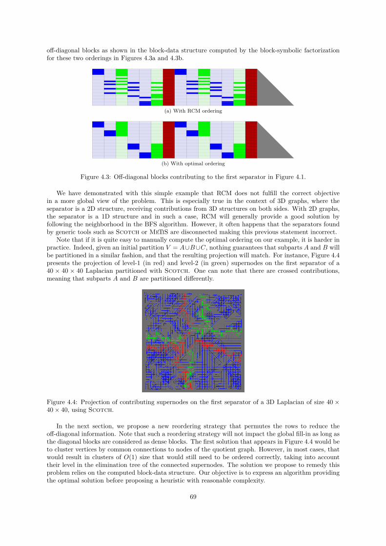
off-diagonal blocks as shown in the block-data structure computed by the block-symbolic factorizationfor these two orderings in Figures 4.3a and 4.3b.

(a) With RCM ordering

(b) With optimal ordering

Figure 4.3: Off-diagonal blocks contributing to the first separator in Figure 4.1.

We have demonstrated with this simple example that RCM does not fulfill the correct objectivein a more global view of the problem. This is especially true in the context of 3D graphs, where theseparator is a 2D structure, receiving contributions from 3D structures on both sides. With 2D graphs,the separator is a 1D structure and in such a case, RCM will generally provide a good solution byfollowing the neighborhood in the BFS algorithm. However, it often happens that the separators foundby generic tools such as Scotch or MeTiS are disconnected making this previous statement incorrect.

Note that if it is quite easy to manually compute the optimal ordering on our example, it is harder inpractice. Indeed, given an initial partition V = A∪B∪C, nothing guarantees that subparts A and B willbe partitioned in a similar fashion, and that the resulting projection will match. For instance, Figure 4.4presents the projection of level-1 (in red) and level-2 (in green) supernodes on the first separator of a40 × 40 × 40 Laplacian partitioned with Scotch. One can note that there are crossed contributions,meaning that subparts A and B are partitioned differently.

Figure 4.4: Projection of contributing supernodes on the first separator of a 3D Laplacian of size 40 ×40× 40, using Scotch.

In the next section, we propose a new reordering strategy that permutes the rows to reduce theoff-diagonal information. Note that such a reordering strategy will not impact the global fill-in as long asthe diagonal blocks are considered as dense blocks. The first solution that appears in Figure 4.4 would beto cluster vertices by common connections to nodes of the quotient graph. However, in most cases, thatwould result in clusters of O(1) size that would still need to be ordered correctly, taking into accounttheir level in the elimination tree of the connected supernodes. The solution we propose to remedy thisproblem relies on the computed block-data structure. Our objective is to express an algorithm providingthe optimal solution before proposing a heuristic with reasonable complexity.

69

4.1.2 Related workStudying the structure of off-diagonal blocks was used in different contexts. In [55], the purpose was toreduce the overhead associated with each single off-diagonal block. The authors proposed a reorderingstrategy that refines the ordering provided by the minimum degree algorithm. Their experiments havebeen applied to 2D graphs and successfully reduce the number of off-diagonal blocks. However, theauthors did not provide a theoretical study of their reordering algorithm and their solution did not applyin the context of 3D graphs. In [134], the authors introduce reordering in the context of a multifrontalsolver. A front is ordered according to its two sons (in the nested dissection process), starting with thelargest son, in order to limit the scatter operation when updating the front with the son’s contributions.A similar approach was studied in [131] for the MUMPS solver, to reorder blocks in order to reduce thecommunication volume induced by the fronts in a distributed context.

4.1.3 Improving the blocking sizeAs presented in section 4.1.1, the RCM algorithm – widely used to order supernodes – generates manyextra diagonal blocks by not considering supernode interactions, which leads to an increased number ofless efficient block operations. In this section, we present an algorithm that reorders supernodes using aglobal view of the nested dissection partition. We expect that considering contributing supernodes willlead to a better quality — a smaller number of larger blocks. Our proposition is to consider the set ofcontributions for each line of a supernode, before using a distance metric to minimize the creation ofoff-diagonal blocks when permuting lines.

Problem modeling

The main idea is to rely on the block-symbolic factorization of L instead of the original graph of A.Indeed, it allows us to take into account fill-in elements that were computed in the block-symbolicfactorization process instead of re-computing those elements with the matrix graph. Let us consider the`th diagonal block C` of the factorized matrix that corresponds to a supernode, and the set of supernodesCk with k < ` corresponding to the supernodes in levels of the elimination tree lower than C`. Note thatwe refer to N as the total number of diagonal blocks appearing in the structure of the factorized matrix,as opposed to n for the total number of unknowns.

We define for each supernode C`:

row`ik ={

1 if vertex i from C` is connected to Ck0 otherwise

, k ∈ J1, `− 1K, i ∈ J1, |C`|K. (4.1)

row`ik is then equal to 1 when the vertex i, or row i, of the supernode C` is connected to any vertexof the supernode k belonging to a lower level in the elimination tree. It is equal to 0, if not, meaningthat no nonzero element connects the two in the initial matrix, or no fill-in will create that connection.Let’s now define for each vertex the set B`i = (row`ik)k∈J1,`−1K. We can then define w`i , the weight of arow i, as in equation (4.2), that represents the number of supernodes contributing to that row i, and thedistance between two rows i and j, d`i,j , as in equation (4.3). It is known as the Hamming distance [66]between two binary vectors, and allows for measuring the number of off-diagonal blocks induced by thesuccession of two rows i and j. Indeed, d`i,j represents the number of off-diagonal blocks that belongs toonly one of the two rows, which can be seen as the number of blocks that end at row i or start at row j.

w`i =`−1∑k=1

row`ik, (4.2)

d`i,j = d(B`i , B`j) =`−1∑k=1

row`ik ⊕ row`jk, (4.3)

where ⊕ is the exclusive or operation.

70

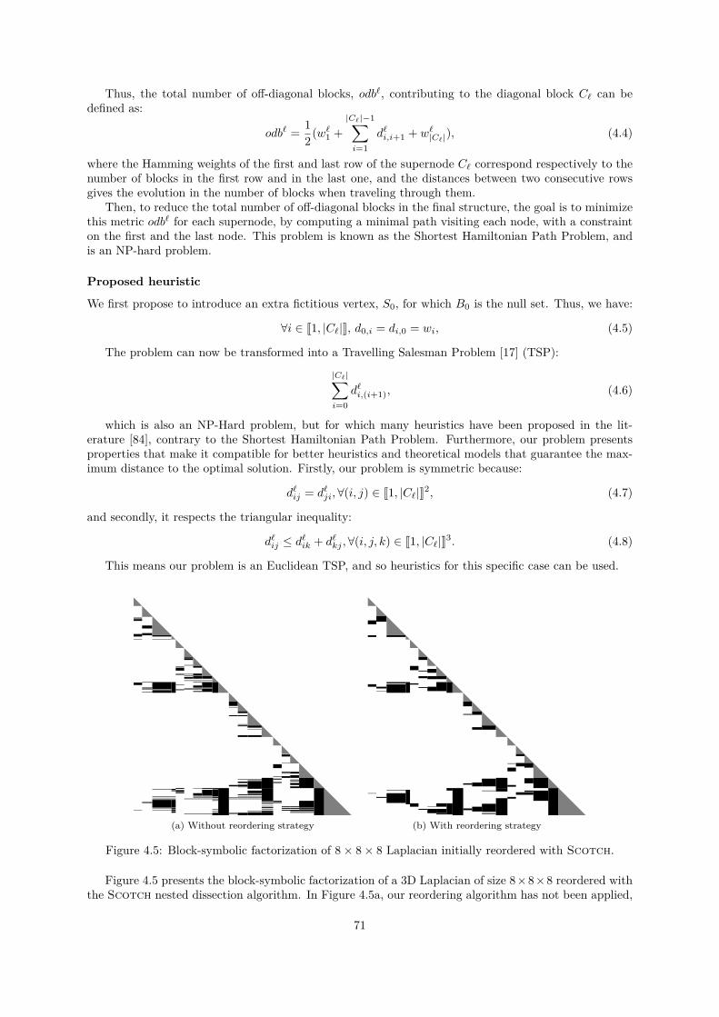
Thus, the total number of off-diagonal blocks, odb`, contributing to the diagonal block C` can bedefined as:

odb` = 12(w`1 +

|C`|−1∑i=1

d`i,i+1 + w`|C`|), (4.4)

where the Hamming weights of the first and last row of the supernode C` correspond respectively to thenumber of blocks in the first row and in the last one, and the distances between two consecutive rowsgives the evolution in the number of blocks when traveling through them.

Then, to reduce the total number of off-diagonal blocks in the final structure, the goal is to minimizethis metric odb` for each supernode, by computing a minimal path visiting each node, with a constrainton the first and the last node. This problem is known as the Shortest Hamiltonian Path Problem, andis an NP-hard problem.

Proposed heuristic

We first propose to introduce an extra fictitious vertex, S0, for which B0 is the null set. Thus, we have:

∀i ∈ J1, |C`|K, d0,i = di,0 = wi, (4.5)

The problem can now be transformed into a Travelling Salesman Problem [17] (TSP):

|C`|∑i=0

d`i,(i+1), (4.6)

which is also an NP-Hard problem, but for which many heuristics have been proposed in the lit-erature [84], contrary to the Shortest Hamiltonian Path Problem. Furthermore, our problem presentsproperties that make it compatible for better heuristics and theoretical models that guarantee the max-imum distance to the optimal solution. Firstly, our problem is symmetric because:

d`ij = d`ji,∀(i, j) ∈ J1, |C`|K2, (4.7)

and secondly, it respects the triangular inequality:

d`ij ≤ d`ik + d`kj ,∀(i, j, k) ∈ J1, |C`|K3. (4.8)

This means our problem is an Euclidean TSP, and so heuristics for this specific case can be used.

(a) Without reordering strategy (b) With reordering strategy

Figure 4.5: Block-symbolic factorization of 8× 8× 8 Laplacian initially reordered with Scotch.

Figure 4.5 presents the block-symbolic factorization of a 3D Laplacian of size 8×8×8 reordered withthe Scotch nested dissection algorithm. In Figure 4.5a, our reordering algorithm has not been applied,

71

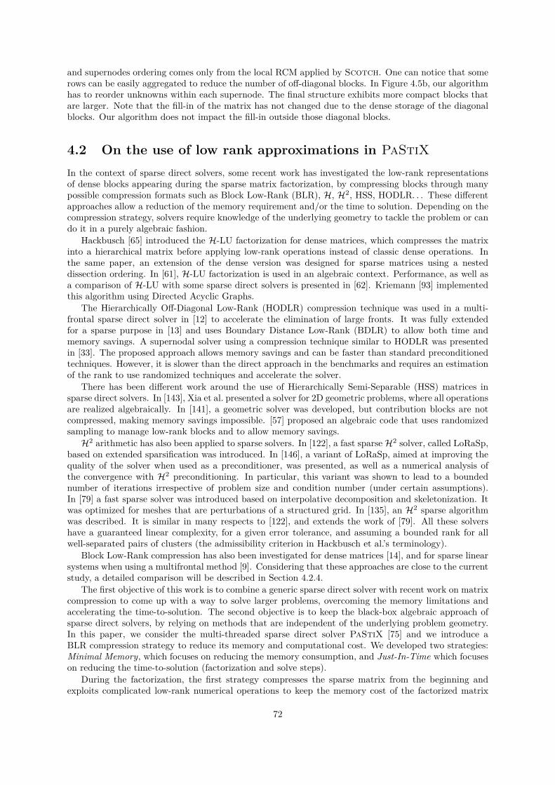
and supernodes ordering comes only from the local RCM applied by Scotch. One can notice that somerows can be easily aggregated to reduce the number of off-diagonal blocks. In Figure 4.5b, our algorithmhas to reorder unknowns within each supernode. The final structure exhibits more compact blocks thatare larger. Note that the fill-in of the matrix has not changed due to the dense storage of the diagonalblocks. Our algorithm does not impact the fill-in outside those diagonal blocks.

4.2 On the use of low rank approximations in PaStiXIn the context of sparse direct solvers, some recent work has investigated the low-rank representationsof dense blocks appearing during the sparse matrix factorization, by compressing blocks through manypossible compression formats such as Block Low-Rank (BLR), H, H2, HSS, HODLR. . . These differentapproaches allow a reduction of the memory requirement and/or the time to solution. Depending on thecompression strategy, solvers require knowledge of the underlying geometry to tackle the problem or cando it in a purely algebraic fashion.

Hackbusch [65] introduced the H-LU factorization for dense matrices, which compresses the matrixinto a hierarchical matrix before applying low-rank operations instead of classic dense operations. Inthe same paper, an extension of the dense version was designed for sparse matrices using a nesteddissection ordering. In [61], H-LU factorization is used in an algebraic context. Performance, as well asa comparison of H-LU with some sparse direct solvers is presented in [62]. Kriemann [93] implementedthis algorithm using Directed Acyclic Graphs.

The Hierarchically Off-Diagonal Low-Rank (HODLR) compression technique was used in a multi-frontal sparse direct solver in [12] to accelerate the elimination of large fronts. It was fully extendedfor a sparse purpose in [13] and uses Boundary Distance Low-Rank (BDLR) to allow both time andmemory savings. A supernodal solver using a compression technique similar to HODLR was presentedin [33]. The proposed approach allows memory savings and can be faster than standard preconditionedtechniques. However, it is slower than the direct approach in the benchmarks and requires an estimationof the rank to use randomized techniques and accelerate the solver.

There has been different work around the use of Hierarchically Semi-Separable (HSS) matrices insparse direct solvers. In [143], Xia et al. presented a solver for 2D geometric problems, where all operationsare realized algebraically. In [141], a geometric solver was developed, but contribution blocks are notcompressed, making memory savings impossible. [57] proposed an algebraic code that uses randomizedsampling to manage low-rank blocks and to allow memory savings.H2 arithmetic has also been applied to sparse solvers. In [122], a fast sparse H2 solver, called LoRaSp,

based on extended sparsification was introduced. In [146], a variant of LoRaSp, aimed at improving thequality of the solver when used as a preconditioner, was presented, as well as a numerical analysis ofthe convergence with H2 preconditioning. In particular, this variant was shown to lead to a boundednumber of iterations irrespective of problem size and condition number (under certain assumptions).In [79] a fast sparse solver was introduced based on interpolative decomposition and skeletonization. Itwas optimized for meshes that are perturbations of a structured grid. In [135], an H2 sparse algorithmwas described. It is similar in many respects to [122], and extends the work of [79]. All these solvershave a guaranteed linear complexity, for a given error tolerance, and assuming a bounded rank for allwell-separated pairs of clusters (the admissibility criterion in Hackbusch et al.’s terminology).

Block Low-Rank compression has also been investigated for dense matrices [14], and for sparse linearsystems when using a multifrontal method [9]. Considering that these approaches are close to the currentstudy, a detailed comparison will be described in Section 4.2.4.

The first objective of this work is to combine a generic sparse direct solver with recent work on matrixcompression to come up with a way to solve larger problems, overcoming the memory limitations andaccelerating the time-to-solution. The second objective is to keep the black-box algebraic approach ofsparse direct solvers, by relying on methods that are independent of the underlying problem geometry.In this paper, we consider the multi-threaded sparse direct solver PaStiX [75] and we introduce aBLR compression strategy to reduce its memory and computational cost. We developed two strategies:Minimal Memory, which focuses on reducing the memory consumption, and Just-In-Time which focuseson reducing the time-to-solution (factorization and solve steps).

During the factorization, the first strategy compresses the sparse matrix from the beginning andexploits complicated low-rank numerical operations to keep the memory cost of the factorized matrix

72

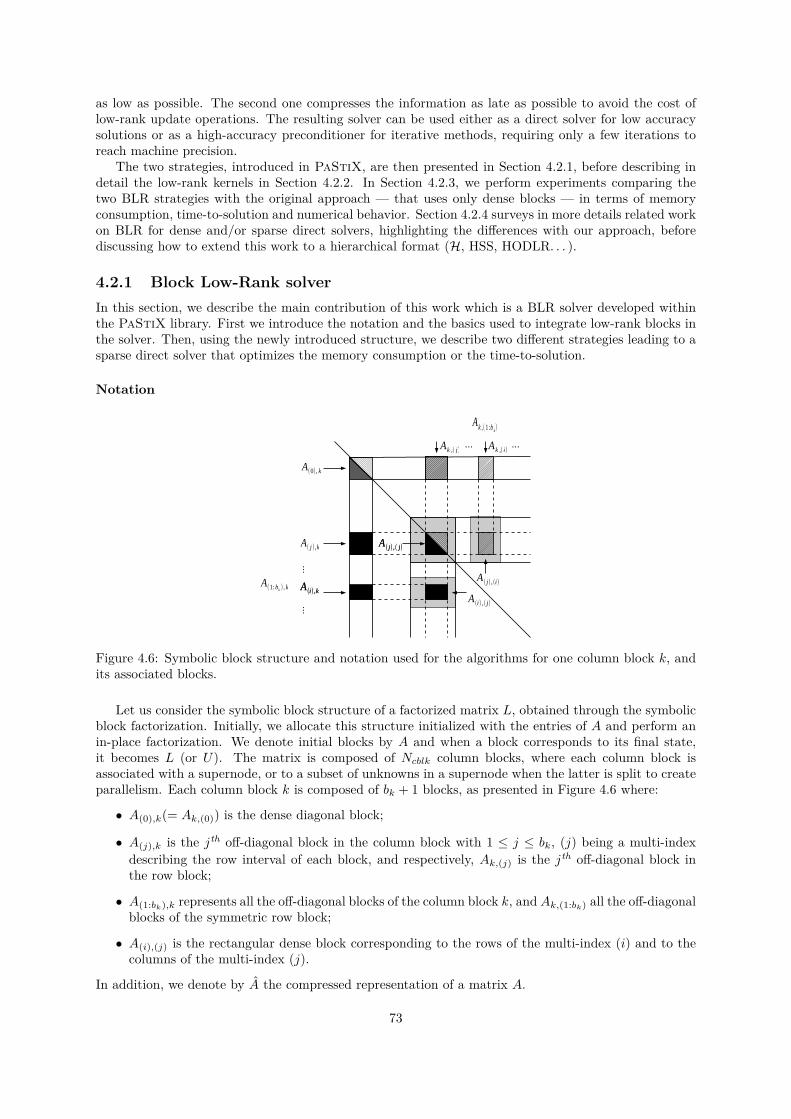
as low as possible. The second one compresses the information as late as possible to avoid the cost oflow-rank update operations. The resulting solver can be used either as a direct solver for low accuracysolutions or as a high-accuracy preconditioner for iterative methods, requiring only a few iterations toreach machine precision.

The two strategies, introduced in PaStiX, are then presented in Section 4.2.1, before describing indetail the low-rank kernels in Section 4.2.2. In Section 4.2.3, we perform experiments comparing thetwo BLR strategies with the original approach — that uses only dense blocks — in terms of memoryconsumption, time-to-solution and numerical behavior. Section 4.2.4 surveys in more details related workon BLR for dense and/or sparse direct solvers, highlighting the differences with our approach, beforediscussing how to extend this work to a hierarchical format (H, HSS, HODLR. . . ).

4.2.1 Block Low-Rank solverIn this section, we describe the main contribution of this work which is a BLR solver developed withinthe PaStiX library. First we introduce the notation and the basics used to integrate low-rank blocks inthe solver. Then, using the newly introduced structure, we describe two different strategies leading to asparse direct solver that optimizes the memory consumption or the time-to-solution.

Notation

...

...

Ak ,(1 :b k)

A(1:bk ) , k

A(0), k

A( j ) ,k

A(i) ,kA(i) ,k

A( j) ,( j)A( j) ,( j)

A(i) ,( j)

A( j) ,(i)

Ak ,( j) Ak ,( i)...

...

Figure 4.6: Symbolic block structure and notation used for the algorithms for one column block k, andits associated blocks.

Let us consider the symbolic block structure of a factorized matrix L, obtained through the symbolicblock factorization. Initially, we allocate this structure initialized with the entries of A and perform anin-place factorization. We denote initial blocks by A and when a block corresponds to its final state,it becomes L (or U). The matrix is composed of Ncblk column blocks, where each column block isassociated with a supernode, or to a subset of unknowns in a supernode when the latter is split to createparallelism. Each column block k is composed of bk + 1 blocks, as presented in Figure 4.6 where:

• A(0),k(= Ak,(0)) is the dense diagonal block;

• A(j),k is the jth off-diagonal block in the column block with 1 ≤ j ≤ bk, (j) being a multi-indexdescribing the row interval of each block, and respectively, Ak,(j) is the jth off-diagonal block inthe row block;

• A(1:bk),k represents all the off-diagonal blocks of the column block k, and Ak,(1:bk) all the off-diagonalblocks of the symmetric row block;

• A(i),(j) is the rectangular dense block corresponding to the rows of the multi-index (i) and to thecolumns of the multi-index (j).

In addition, we denote by A the compressed representation of a matrix A.

73

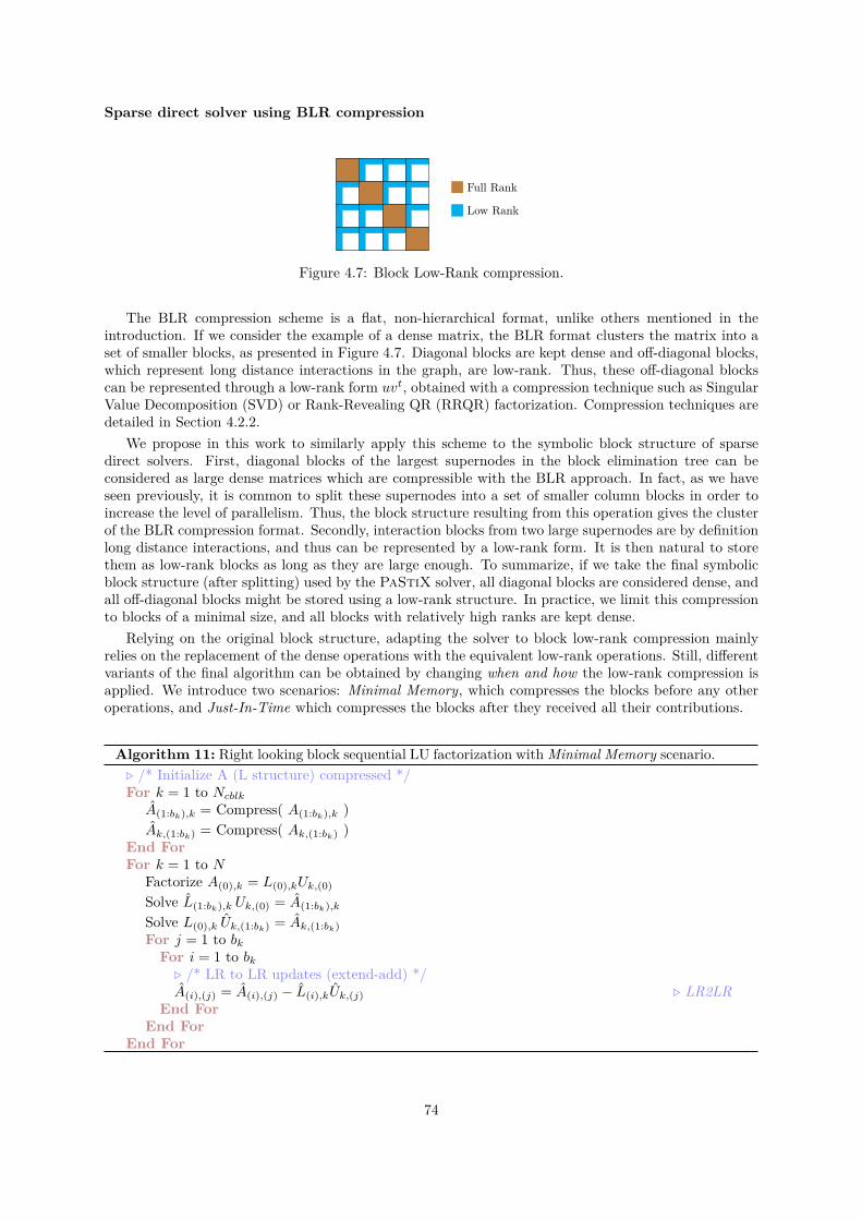
Sparse direct solver using BLR compression

Full Rank

Low Rank

Figure 4.7: Block Low-Rank compression.

The BLR compression scheme is a flat, non-hierarchical format, unlike others mentioned in theintroduction. If we consider the example of a dense matrix, the BLR format clusters the matrix into aset of smaller blocks, as presented in Figure 4.7. Diagonal blocks are kept dense and off-diagonal blocks,which represent long distance interactions in the graph, are low-rank. Thus, these off-diagonal blockscan be represented through a low-rank form uvt, obtained with a compression technique such as SingularValue Decomposition (SVD) or Rank-Revealing QR (RRQR) factorization. Compression techniques aredetailed in Section 4.2.2.

We propose in this work to similarly apply this scheme to the symbolic block structure of sparsedirect solvers. First, diagonal blocks of the largest supernodes in the block elimination tree can beconsidered as large dense matrices which are compressible with the BLR approach. In fact, as we haveseen previously, it is common to split these supernodes into a set of smaller column blocks in order toincrease the level of parallelism. Thus, the block structure resulting from this operation gives the clusterof the BLR compression format. Secondly, interaction blocks from two large supernodes are by definitionlong distance interactions, and thus can be represented by a low-rank form. It is then natural to storethem as low-rank blocks as long as they are large enough. To summarize, if we take the final symbolicblock structure (after splitting) used by the PaStiX solver, all diagonal blocks are considered dense, andall off-diagonal blocks might be stored using a low-rank structure. In practice, we limit this compressionto blocks of a minimal size, and all blocks with relatively high ranks are kept dense.

Relying on the original block structure, adapting the solver to block low-rank compression mainlyrelies on the replacement of the dense operations with the equivalent low-rank operations. Still, differentvariants of the final algorithm can be obtained by changing when and how the low-rank compression isapplied. We introduce two scenarios: Minimal Memory, which compresses the blocks before any otheroperations, and Just-In-Time which compresses the blocks after they received all their contributions.

Algorithm 11: Right looking block sequential LU factorization withMinimal Memory scenario.. /* Initialize A (L structure) compressed */For k = 1 to Ncblk

A(1:bk),k = Compress( A(1:bk),k )Ak,(1:bk) = Compress( Ak,(1:bk) )

End ForFor k = 1 to N

Factorize A(0),k = L(0),kUk,(0)

Solve L(1:bk),k Uk,(0) = A(1:bk),k

Solve L(0),k Uk,(1:bk) = Ak,(1:bk)For j = 1 to bkFor i = 1 to bk. /* LR to LR updates (extend-add) */A(i),(j) = A(i),(j) − L(i),kUk,(j) . LR2LR

End ForEnd For

End For

74

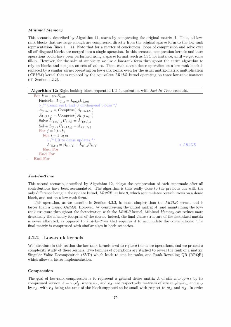
Minimal Memory

This scenario, described by Algorithm 11, starts by compressing the original matrix A. Thus, all low-rank blocks that are large enough are compressed directly from the original sparse form to the low-rankrepresentation (lines 1 − 4). Note that for a matter of conciseness, loops of compression and solve overall off-diagonal blocks are merged into a single operation. In this scenario, compression kernels and lateroperations could have been performed using a sparse format, such as CSC for instance, until we get somefill-in. However, for the sake of simplicity we use a low-rank form throughout the entire algorithm torely on blocks and not just on sets of values. Then, each classic dense operation on a low-rank block isreplaced by a similar kernel operating on low-rank forms, even for the usual matrix-matrix multiplication(GEMM ) kernel that is replaced by the equivalent LR2LR kernel operating on three low-rank matrices(cf. Section 4.2.2).

Algorithm 12: Right looking block sequential LU factorization with Just-In-Time scenario.For k = 1 to Ncblk

Factorize A(0),k = L(0),kUk,(0). /* Compress L and U off-diagonal blocks */A(1:bk),k = Compress( A(1:bk),k )Ak,(1:bk) = Compress( Ak,(1:bk) )Solve L(1:bk),k Uk,(0) = A(1:bk),k

Solve L(0),k Uk,(1:bk) = Ak,(1:bk)For j = 1 to bkFor i = 1 to bk. /* LR to dense updates */A(i),(j) = A(i),(j) − L(i),kUk,(j) . LR2GE

End ForEnd For

End For

Just-In-Time

This second scenario, described by Algorithm 12, delays the compression of each supernode after allcontributions have been accumulated. The algorithm is thus really close to the previous one with theonly difference being in the update kernel, LR2GE , at line 9, which accumulates contributions on a denseblock, and not on a low-rank form.

This operation, as we describe in Section 4.2.2, is much simpler than the LR2LR kernel, and isfaster than a classic GEMM. However, by compressing the initial matrix A, and maintaining the low-rank structure throughout the factorization with the LR2LR kernel, Minimal Memory can reduce moredrastically the memory footprint of the solver. Indeed, the final dense structure of the factorized matrixis never allocated, as opposed to Just-In-Time that requires it to accumulate the contributions. Thefinal matrix is compressed with similar sizes in both scenarios.

4.2.2 Low-rank kernelsWe introduce in this section the low-rank kernels used to replace the dense operations, and we present acomplexity study of these kernels. Two families of operations are studied to reveal the rank of a matrix:Singular Value Decomposition (SVD) which leads to smaller ranks, and Rank-Revealing QR (RRQR)which allows a faster implementation.

Compression

The goal of low-rank compression is to represent a general dense matrix A of size mA-by-nA by itscompressed version A = uAv

tA, where uA, and vA, are respectively matrices of size mA-by-rA, and nA-

by-rA, with rA being the rank of the block supposed to be small with respect to mA and nA. In order

75

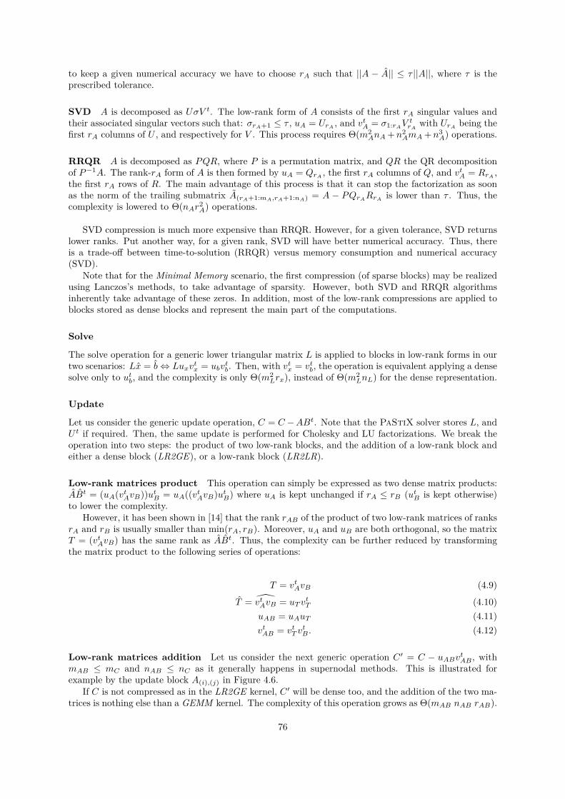
to keep a given numerical accuracy we have to choose rA such that ||A − A|| ≤ τ ||A||, where τ is theprescribed tolerance.

SVD A is decomposed as UσV t. The low-rank form of A consists of the first rA singular values andtheir associated singular vectors such that: σrA+1 ≤ τ , uA = UrA

, and vtA = σ1:rAV trA

with UrAbeing the

first rA columns of U , and respectively for V . This process requires Θ(m2AnA +n2

AmA +n3A) operations.

RRQR A is decomposed as PQR, where P is a permutation matrix, and QR the QR decompositionof P−1A. The rank-rA form of A is then formed by uA = QrA

, the first rA columns of Q, and vtA = RrA,

the first rA rows of R. The main advantage of this process is that it can stop the factorization as soonas the norm of the trailing submatrix A(rA+1:mA,rA+1:nA) = A − PQrA

RrAis lower than τ . Thus, the

complexity is lowered to Θ(nAr2A) operations.

SVD compression is much more expensive than RRQR. However, for a given tolerance, SVD returnslower ranks. Put another way, for a given rank, SVD will have better numerical accuracy. Thus, thereis a trade-off between time-to-solution (RRQR) versus memory consumption and numerical accuracy(SVD).

Note that for the Minimal Memory scenario, the first compression (of sparse blocks) may be realizedusing Lanczos’s methods, to take advantage of sparsity. However, both SVD and RRQR algorithmsinherently take advantage of these zeros. In addition, most of the low-rank compressions are applied toblocks stored as dense blocks and represent the main part of the computations.

Solve

The solve operation for a generic lower triangular matrix L is applied to blocks in low-rank forms in ourtwo scenarios: Lx = b⇔ Luxv

tx = ubv

tb. Then, with vtx = vtb, the operation is equivalent applying a dense

solve only to utb, and the complexity is only Θ(m2Lrx), instead of Θ(m2

LnL) for the dense representation.

Update

Let us consider the generic update operation, C = C −ABt. Note that the PaStiX solver stores L, andU t if required. Then, the same update is performed for Cholesky and LU factorizations. We break theoperation into two steps: the product of two low-rank blocks, and the addition of a low-rank block andeither a dense block (LR2GE), or a low-rank block (LR2LR).

Low-rank matrices product This operation can simply be expressed as two dense matrix products:ABt = (uA(vtAvB))utB = uA((vtAvB)utB) where uA is kept unchanged if rA ≤ rB (utB is kept otherwise)to lower the complexity.

However, it has been shown in [14] that the rank rAB of the product of two low-rank matrices of ranksrA and rB is usually smaller than min(rA, rB). Moreover, uA and uB are both orthogonal, so the matrixT = (vtAvB) has the same rank as ABt. Thus, the complexity can be further reduced by transformingthe matrix product to the following series of operations:

T = vtAvB (4.9)

T = vtAvB = uT vtT (4.10)

uAB = uAuT (4.11)vtAB = vtT v

tB . (4.12)

Low-rank matrices addition Let us consider the next generic operation C ′ = C − uABvtAB , withmAB ≤ mC and nAB ≤ nC as it generally happens in supernodal methods. This is illustrated forexample by the update block A(i),(j) in Figure 4.6.

If C is not compressed as in the LR2GE kernel, C ′ will be dense too, and the addition of the two ma-trices is nothing else than a GEMM kernel. The complexity of this operation grows as Θ(mAB nAB rAB).

76

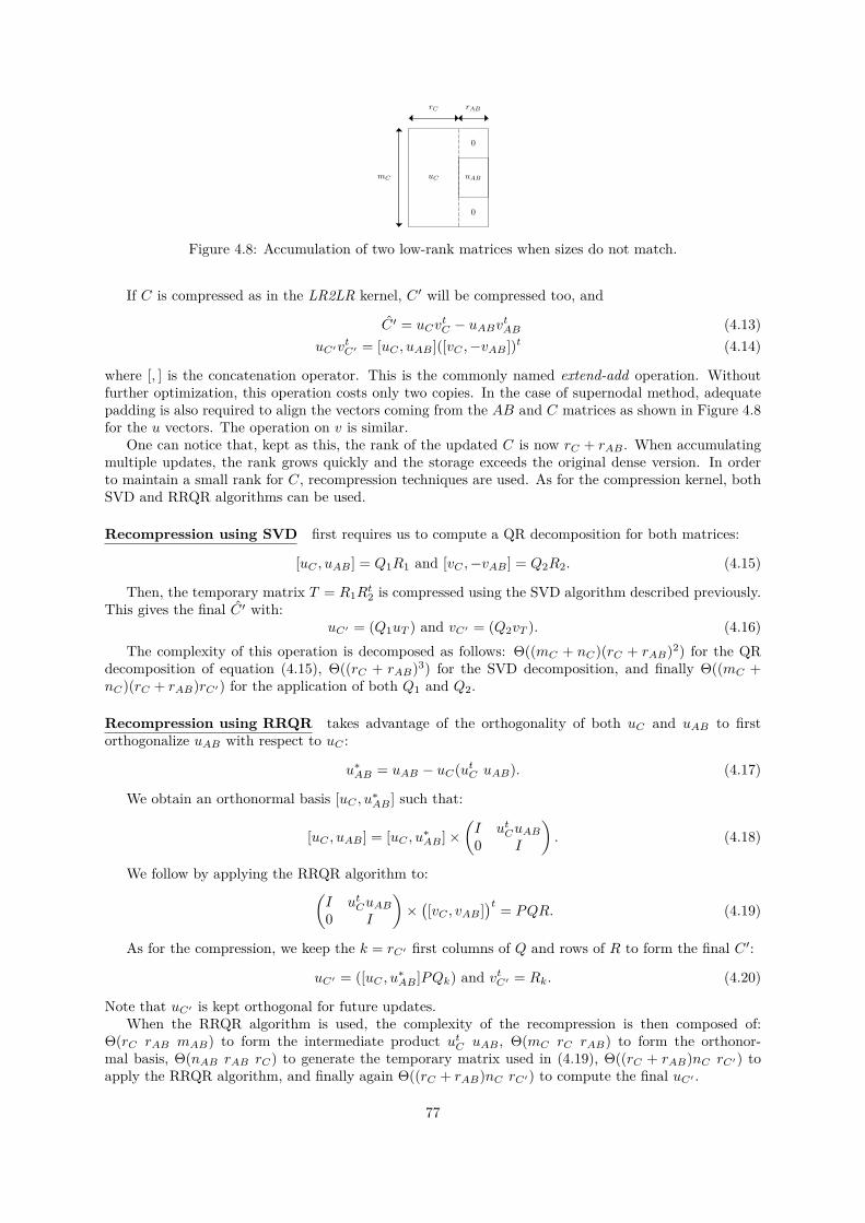
uC uABmC

rC rAB

0

0

Figure 4.8: Accumulation of two low-rank matrices when sizes do not match.

If C is compressed as in the LR2LR kernel, C ′ will be compressed too, and

C ′ = uCvtC − uABvtAB (4.13)

uC′vtC′ = [uC , uAB ]([vC ,−vAB ])t (4.14)

where [, ] is the concatenation operator. This is the commonly named extend-add operation. Withoutfurther optimization, this operation costs only two copies. In the case of supernodal method, adequatepadding is also required to align the vectors coming from the AB and C matrices as shown in Figure 4.8for the u vectors. The operation on v is similar.

One can notice that, kept as this, the rank of the updated C is now rC + rAB . When accumulatingmultiple updates, the rank grows quickly and the storage exceeds the original dense version. In orderto maintain a small rank for C, recompression techniques are used. As for the compression kernel, bothSVD and RRQR algorithms can be used.

Recompression using SVD first requires us to compute a QR decomposition for both matrices:

[uC , uAB ] = Q1R1 and [vC ,−vAB ] = Q2R2. (4.15)

Then, the temporary matrix T = R1Rt2 is compressed using the SVD algorithm described previously.

This gives the final C ′ with:uC′ = (Q1uT ) and vC′ = (Q2vT ). (4.16)

The complexity of this operation is decomposed as follows: Θ((mC + nC)(rC + rAB)2) for the QRdecomposition of equation (4.15), Θ((rC + rAB)3) for the SVD decomposition, and finally Θ((mC +nC)(rC + rAB)rC′) for the application of both Q1 and Q2.

Recompression using RRQR takes advantage of the orthogonality of both uC and uAB to firstorthogonalize uAB with respect to uC :

u∗AB = uAB − uC(utC uAB). (4.17)

We obtain an orthonormal basis [uC , u∗AB ] such that:

[uC , uAB ] = [uC , u∗AB ]×(I utCuAB0 I

). (4.18)

We follow by applying the RRQR algorithm to:(I utCuAB0 I

)×([vC , vAB ]

)t = PQR. (4.19)

As for the compression, we keep the k = rC′ first columns of Q and rows of R to form the final C ′:

uC′ = ([uC , u∗AB ]PQk) and vtC′ = Rk. (4.20)

Note that uC′ is kept orthogonal for future updates.When the RRQR algorithm is used, the complexity of the recompression is then composed of:

Θ(rC rAB mAB) to form the intermediate product utC uAB , Θ(mC rC rAB) to form the orthonor-mal basis, Θ(nAB rAB rC) to generate the temporary matrix used in (4.19), Θ((rC + rAB)nC rC′) toapply the RRQR algorithm, and finally again Θ((rC + rAB)nC rC′) to compute the final uC′ .

77

Summary

Table 4.1 presents the computational complexity for the two low-rank strategies with respect to theoriginal version of the solver. To get the main factor of the complexity, we make the assumption thatmC ≥ mA ≥ mB , rA ≥ rB , mC ≥ nC , and rC ≤ rC′ . One can note that the Just-In-Time strategyperforms the calculation of the low-rank contribution before assembling the matrix explicitly to applya dense modification. The main factor of the complexity does not depend on nA but on the ranks rAand rB : there are fewer operations to be performed. On the other hand, the Minimal Memory strategyrequires using either the SVD or RRQR recompression, for which the complexity depends on mC andnC , the dimensions of the block C. This explains why this strategy is of higher complexity than theoriginal solver.

When considering dense matrices, a low-rank matrix is usually modified by a contribution of the samesize: the low-rank extend-add process may be efficient and lead to performance gain [14]. It is also thecase for the CUFS strategy in BLR-MUMPS, which compresses a dense front before applying operationsbetween low-rank blocks of the same size.

In our case, a block C receives many small contributions as stated by the separator theorem [101]describing how the size of supernodes is evolving during the nested dissection process. According to ourexperiments, it is still interesting to have low-rank blocks at the end of the factorization, meaning thatranks remain lower than min(mC , nC)/4 (otherwise compression will not help), even if blocks received alarge number of contributions. Thus, rC′ is often close to or equal to rC and lower than rC+rAB : the rankis often invariant to applying a small contribution. So it is less expensive to use RRQR recompression(and operations are more suitable for the performance). In terms of complexity, the recompressiondepends on the size of the target block C and not on the size of the contribution blocks A and B. Ashuge low-rank blocks are recompressed many times, it makes the Minimal Memory scenario slower thanthe dense version, but allows consequent memory savings.

Finally, the main advantage of the Minimal Memory scenario is that it can drastically reduce thememory footprint of the solver, since it compresses the matrix before the factorization. Thus, the finalstructure of the dense factorized matrix is never allocated, and the low-rank structure needs to bemaintained throughout the factorization process to lower the memory peak.

In order to overcome the issue of expensive low-rank additions, an idea would be to consider random-ized techniques to allow an extend-add process depending on the size of contributing blocks and not onthe size of the target block.

4.2.3 Numerical experimentsExperiments were conducted on the Plafrim1 supercomputer, and more precisely on the miriel cluster.Each node is equipped with two Intel Xeon E5-2680 v3 12-cores running at 2.50 GHz and 128 GB ofmemory. The Intel MKL 2016 is used for BLAS and SVD kernels. The RRQR kernel is coming fromthe BLR-MUMPS solver [9], and is an extension of the block rank-revealing QR factorization subroutinesfrom LAPACK 3.6.0 (xGEQP3).

The PaStiX version used for our experiments is available on the public git repository2 as the tagpapers/pdsec17. The multi-threaded version used is the static scheduling version presented in [95].

For the initial ordering step, we used Scotch [118] 5.1.11 with the configurable strategy string fromPaStiX to set the minimal size of non separated subgraphs, cmin, to 15. We also set the frat parameterto 0.08, meaning that column aggregation is allowed by Scotch as long as the fill-in introduced doesnot exceed 8% of the original matrix.

In experiments, blocks that are larger than 256 are split into blocks of size at most 128 to create moreparallelism while keeping sizes large enough. The same 128 criteria is used to define the minimal widthof the column blocks that are compressible. An additional limit on the minimal height to compress anoff-diagonal block is set to 20.

Experiments were computed on a set of 3D matrices from The SuiteSparse Matrix Collection [43]:

• Atmosmodj: atmospheric model (1 270 432 dofs)

• Audi: structural problem (943 695 dofs)1https://plafrim.bordeaux.inria.fr2https://gitlab.inria.fr/solverstack/pastix

78

• Hook: model of a steel hook (1 498 023 dofs)

• Serena: gas reservoir simulation (1 391 349 dofs)

• Geo1438 : geomechanical model of earth (1 437 960 dofs)

We also used 3D Laplacian generators (7 points stencils), and defined lap120 as a Laplacian of size1203. Note that when results showing numerical precision are presented, we used the backward error onb: ||Ax−b||2||b||2 .

SVD versus RRQR

The first experiment studies the behavior of the two compression methods coupled with both MinimalMemory, and Just-In-Time scenarios, on the matrix Atmosmodj. Table 4.2 presents the sequentialtimings of each operation of the numerical factorization with a tolerance of 10−8, as well as the memoryused to store the final structure of the factorized matrix.

We can first notice that SVD compression kernels are much more time consuming than the RRQRkernels in both scenarios following the complexity study from Section 4.2.2. Indeed, RRQR compressionkernels stop the computations as soon as the rank is found which reduces by a large factor the complexity,and this reduction is reflected in the time-to-solution. However, the SVD allows, for a given tolerance,to get a better memory reduction in both scenarios.

Comparing the Minimal Memory and the Just-In-Time scenario, the compression time is minimizedin the Minimal Memory scenario because the compression occurs on the initial blocks which hold morezeros and are lower rank than when they have been updated. The time for the update addition, extend-add operation, becomes dominant in the Minimal Memory scenario, and even explodes when SVD isused. This is expected as the complexity depends on the largest blocks in the addition even for smallcontributions (see Section 4.2.2). Note that this ratio will evolve in favor of the extend-add operation onlarger matrices where the ratio of updates of same size becomes dominant with respect to the number ofupdates from small blocks. For both compression methods, both scenarios compress the final coefficientswith similar rates.

The diagonal block factorization time is invariant in the five strategies: the block sizes and kernelsare identical. Panel solve, update product, and solve times are reduced in all low-rank configurationscompared to the dense factorization and the timings follow the final size of the factors, since this sizereflects the final ranks of the blocks.

To conclude, the Minimal Memory scenario is not able to compete with the original direct factoriza-tion due to the costly update addition. However, it reduced the memory peak of the solver to the finalsize of the factors. The Minimal Memory/RRQR offers a 25% memory reduction while doubling thesequential time-to-solution. The Just-In-Time scenario competes with the original direct factorization,and divides by two the time-to-solution with RRQR kernels.

Performance

Figure 4.9 presents the overall performance achieved by the two low-rank scenarios with respect to theoriginal version of the solver (where lower is better) on the previously introduced set of 6 matrices. Allversions are multi-threaded implementations and use all the 24 cores of one node. The scheduling used isthe PaStiX static scheduler developed for the original version, this might have a negative impact on thelow-rank implementations by creating a load imbalance. We study only the RRQR kernels as the SVDkernels have shown to be much slower. Three tolerance thresholds are studied for their impact on thetime-to-solution, and the accuracy of the first residual of the solver, which went through one refinementstep is shown with the backward errors printed on top of each bar.

Figure 4.9a shows that the Just-In-Time/RRQR scenario is able to reduce the time-to-solution inalmost all cases of tolerance, and for all matrices which have a large spectrum of numerical properties.These results show that applications which requires low accuracy, as the seismic application for instance,can benefit by up to a factor of 3.3. Figure 4.9b shows that it is more difficult for the Minimal Mem-ory/RRQR scenario to be competitive. The performance is always degraded with respect to the originalPaStiX performance, with an average loss of around a factor of 1.8, and the tolerance has a much lowerimpact than for the previous case.

79

lap120 atmosmodj audi Geo1438 Hook Serena0.0

0.2

0.4

0.6

0.8

1.0

1.2

1.4

1.6

Tim

e B

LR

/ T

ime

PaS

tiX

1.0e-

05

6.7

e-10

1.9

e-14

1.0

e-05 4.6e-

10

1.6

e-14

9.4

e-04

3.4e-

09

8.9e

-17

7.3e-

05

1.8e-

08

2.4

e-12

2.3

e-04

8.3e

-10 3

.6e-

15

5.2

e-05

1.2e-

08

1.2e

-12

τ =10−4

τ =10−8

τ =10−12

(a) Just-In-Time scenario using RRQR.

lap120 atmosmodj audi Geo1438 Hook Serena0.0

0.5

1.0

1.5

2.0

2.5

3.0

3.5

Tim

e B

LR

/ T

ime

PaS

tiX

8.9e

-05

2.0e

-08

4.6e

-13

1.1e

-04

9.8e

-09

3.7e

-13

3.5e

-03

8.9e

-07

1.6e-

10

5.8e

-04

2.7e

-07

1.9e

-11

1.9e-

04

1.1

e-07

1.7e-

12

3.6e

-04 2.

3e-0

7

3.7e

-11

τ =10−4

τ =10−8

τ =10−12

(b) Minimal Memory scenario using RRQR.

Figure 4.9: Performance of both strategies with 3 tolerance thresholds, backward error of the solution isprinted on top of each bar.

80

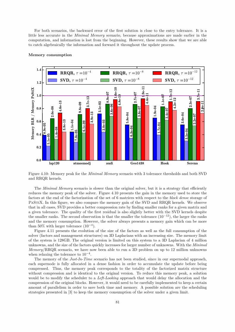
For both scenarios, the backward error of the first solution is close to the entry tolerance. It is alittle less accurate in the Minimal Memory scenario, because approximations are made earlier in thecomputation, and information is lost from the beginning. However, these results show that we are ableto catch algebraically the information and forward it throughout the update process.

Memory consumption

lap120 atmosmodj audi Geo1438 Hook Serena0.0

0.2

0.4

0.6

0.8

1.0

1.2

1.4

Mem

ory B

LR

/ M

emory

PaS

tiX

8.9e

-05

5.1

e-05

2.0e

-08

1.4e-

08

4.6e-

133.8

e-13

1.1

e-04

7.0e

-05

9.8e-

09

6.1e-

09

3.7e-

13

3.9

e-13 3.

5e-

03

2.0

e-03

8.9e-

073.

6e-

06

1.6e-

104.

8e-

10

5.8e

-04

6.3e

-04

2.7

e-07

3.6e-

07

1.9

e-11

4.4

e-11

1.9e-

04

1.7e

-04

1.1

e-07

2.4

e-07

1.7

e-12

4.2

e-12

3.6e

-04

3.5

e-04

2.3

e-07

2.2e

-07

3.7

e-11

2.8e-

11

RRQR, τ =10−4

SVD, τ =10−4

RRQR, τ =10−8

SVD, τ =10−8

RRQR, τ =10−12

SVD, τ =10−12

Figure 4.10: Memory peak for the Minimal Memory scenario with 3 tolerance thresholds and both SVDand RRQR kernels.

The Minimal Memory scenario is slower than the original solver, but it is a strategy that efficientlyreduces the memory peak of the solver. Figure 4.10 presents the gain in the memory used to store thefactors at the end of the factorization of the set of 6 matrices with respect to the block dense storage ofPaStiX. In this figure, we also compare the memory gain of the SVD and RRQR kernels. We observethat in all cases, SVD provides a better compression rate by finding smaller ranks for a given matrix anda given tolerance. The quality of the first residual is also slightly better with the SVD kernels despitethe smaller ranks. The second observation is that the smaller the tolerance (10−12), the larger the ranksand the memory consumption. However, the solver always presents a memory gain which can be morethan 50% with larger tolerance (10−4).

Figure 4.11 presents the evolution of the size of the factors as well as the full consumption of thesolver (factors and management structures) on 3D Laplacians with an increasing size. The memory limitof the system is 128GB. The original version is limited on this system to a 3D Laplacian of 4 millionunknowns, and the size of the factors quickly increases for larger number of unknowns. With the MinimalMemory/RRQR scenario, we have now been able to run a 3D problem on up to 12 million unknownswhen relaxing the tolerance to 10−4.

The memory of the Just-In-Time scenario has not been studied, since in our supernodal approach,each supernode is fully allocated in a dense fashion in order to accumulate the update before beingcompressed. Thus, the memory peak corresponds to the totality of the factorized matrix structurewithout compression and is identical to the original version. To reduce this memory peak, a solutionwould be to modify the scheduler to a Left-Looking approach that would delay the allocation and thecompression of the original blocks. However, it would need to be carefully implemented to keep a certainamount of parallelism in order to save both time and memory. A possible solution are the schedulingstrategies presented in [3] to keep the memory consumption of the solver under a given limit.

81

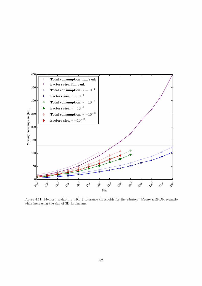
100

3

110

3

120

3

130

3

140

3

150

3

160

3

170

3

180

3

190

3

200

3

210

3

220

3

230

3

Size

0

50

100

150

200

250

300

350

400

Mem

ory c

onsu

mpti

on (

GB

)

Total consumption, full rank

Factors size, full rank

Total consumption, τ =10−4

Factors size, τ =10−4

Total consumption, τ =10−8

Factors size, τ =10−8

Total consumption, τ =10−12

Factors size, τ =10−12

Figure 4.11: Memory scalability with 3 tolerance thresholds for the Minimal Memory/RRQR scenariowhen increasing the size of 3D Laplacians.

82

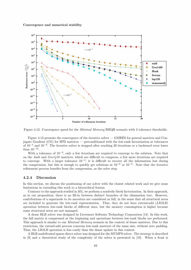
Convergence and numerical stability

0 5 10 15 20

Number of refinement iterations

10-14

10-13

10-12

10-11

10-10

10-9

10-8

10-7

10-6

10-5

10-4

10-3

10-2

Bac

kw

ard e

rror:

||Ax−b||

2

||b|| 2

τ =10−4

τ =10−8

audi

Geo1438

Hook

Serena

lap120

atmosmodj

Figure 4.12: Convergence speed for the Minimal Memory/RRQR scenario with 2 tolerance thresholds.

Figure 4.12 presents the convergence of the iterative solver — GMRES for general matrices and Con-jugate Gradient (CG) for SPD matrices — preconditioned with the low-rank factorization at tolerancesof 10−4 and 10−8. The iterative solver is stopped after reaching 20 iterations or a backward error lowerthan 10−12.

With a tolerance of 10−8, only a few iterations are required to converge to the solution. Note thaton the Audi and Geo1438 matrices, which are difficult to compress, a few more iterations are requiredto converge. With a larger tolerance 10−4, it is difficult to recover all the information lost duringthe compression, but this is enough to quickly get solutions at 10−6 or 10−8. Note that the iterativerefinement process benefits from the compression, as the solve step.

4.2.4 DiscussionIn this section, we discuss the positioning of our solver with the closest related work and we give somelimitations in extending this work to a hierarchical format.

Contrary to the approach studied in [65], we perform a symbolic block factorization. In their approach,as in our proposition, there is no fill-in between distinct branches of the elimination tree. However,contributions of a supernode to its ancestors are considered as full, in the sense that all structural zerosare included to generate the low-rank representation. Thus, they do not have extend-add (LR2LR)operation between low-rank blocks of different sizes, but the memory consumption is higher becausesome structural zeros are not managed.

A dense BLR solver was designed by Livermore Software Technology Corporation [14]. In this work,the full matrix is compressed at the beginning and operations between low-rank blocks are performed.This approach is similar to our Minimal Memory scenario in the context of dense matrices. Due to thisrestriction, the extend-add process concerns low-rank matrices of the same size, without zero padding.Thus, the LR2LR operation is less costly than the dense update in this context.

A BLRmultifrontal sparse direct solver was designed for the MUMPS solver. The strategy is describedin [9] and a theoretical study of the complexity of the solver is presented in [10]. When a front is

83

eliminated, different strategies are proposed to enhance the time-to-solution. Our scenario Just-In-Timeis close to their FCSU (Factor, Compress, Solve, Update) strategy. The LUAR (Low-Rank UpdateAccumulation with Recompression) groups together multiple low-rank products to exploit the memorylocality during the product recompression process. This could be similarly used in the Just-In-Time, butwould imply larger ranks in the extend-add operations of the Minimal Memory. The CUFS (Compress,Update, Factor, Solve) is the strategy closest to our Minimal Memory scenario. However, only a densefront is fully compressed before being eliminated: contributing blocks are not compressed and low-rankoperations occur within a dense matrix similarly to the previous work from LSTC. If the time-to-solutionis better with BLR-MUMPS, there is more room for memory savings in our approach.

With the aim of extending our solver to hierarchical compression schemes, such as H, HSS, orHODLR, we consider graphs coming from finite-element meshes from real-life simulations of 3D physicalproblems. From a theoretical point of view, the majority of these graphs have a bounded degree, andthus good separators respecting the separator theorems [101] can be built. For a n-vertices mesh, thetime complexity of a direct solver is in Θ(n2), and we expect to build a low-rank solver requiring Θ(n 4

3 )operations. For the memory requirements, the direct approach leads to an overall storage of Θ(n 4

3 ), whilewe target a Θ(n log(n)) complexity. Let us consider the last separator of size Θ(n 2

3 ) for a 3D mesh, andone of the largest low-rank blocks of this separator. They are asymptotically the same size. Previousstudies have shown that such a block may have a rank of order Θ(n 1

3 ).For the Minimal Memory scenario, we have seen that the time-to-solution is longer than the dense

version. As low-rank blocks become larger in the hierarchy, it will be even worse than the solution wedeveloped. For the Just-In-Time scenario, maintaining such a block in a dense form before compressingthe block requires Θ(n 4

3 ) memory and does not satisfy the memory complexity we target. It also meansthat a compromise between Minimal Memory and Just-In-Time strategies using a Left-Looking approachmight not be a relevant solution. Currently, no sparse solver is able to perform efficiently the extend-addoperations using compression techniques such as SVD or RRQR, and it is still an open problem.

84

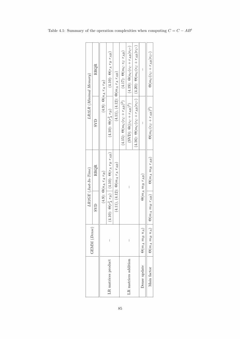
Table 4.1: Summary of the operation complexities when computing C = C −ABt

GEM

M(D

ense)

LR2G

E(Just-In-T

ime)

LR2L

R(M

inim

alMem

ory)

SVD

RRQR

SVD

RRQR

LRmatric

esprod

uct

−(4.9):

Θ(nAr A

r B)

(4.9):

Θ(nAr A

r B)

(4.10):

Θ(r

2 Ar B

)(4.10):

Θ(rAr B

r AB

)(4.10):

Θ(r

2 Ar B

)(4.10):

Θ(rAr B

r AB

)(4.11),(4.12

):Θ

(mAr A

r AB

)(4.11),(4.12

):Θ

(mAr A

r AB

)

LRmatric

esad

ditio

n−

−(4.15):

Θ(m

C(rC

+r AB

)2 )(4.17):

Θ(m

Cr C

r AB

)(SVD):

Θ((r C

+r AB

)3 )(4.19):

Θ(nC

(rC

+r AB

)rC

′ )(4.16):

Θ(m

C(rC

+r AB

)rC

′ )(4.20):

Θ(m

C(rC

+r AB

)rC

′ )Den

seup

date

Θ(m

AmBnA

)Θ

(mAmBr AB

)−

−

Mainfactor

Θ(m

AmBnA

)Θ

(mAmBr AB

)Θ

(mAmBr AB

)Θ

(mC

(rC

+r AB

)2 )Θ

(mC

(rC

+r AB

)rC

′ )

85

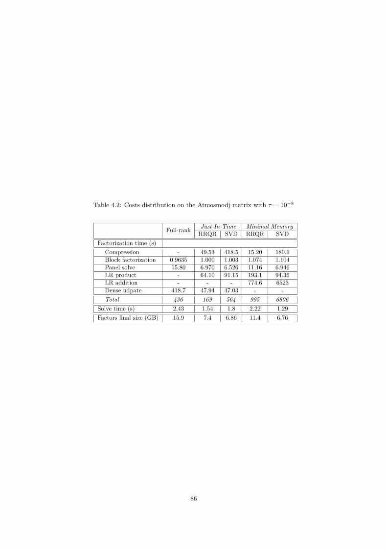
Table 4.2: Costs distribution on the Atmosmodj matrix with τ = 10−8

Full-rank Just-In-Time Minimal MemoryRRQR SVD RRQR SVD

Factorization time (s)Compression - 49.53 418.5 15.20 180.9Block factorization 0.9635 1.000 1.003 1.074 1.104Panel solve 15.80 6.970 6.526 11.16 6.946LR product - 64.10 91.15 193.1 94.36LR addition - - - 774.6 6523Dense udpate 418.7 47.94 47.03 - -Total 436 169 564 995 6806

Solve time (s) 2.43 1.54 1.8 2.22 1.29Factors final size (GB) 15.9 7.4 6.86 11.4 6.76

86

Conclusion

I In Chapter 2, we presented a new implementation of a sparse direct solver with a supernodal methodusing a task-based programming paradigm. The programming paradigm shift insulates the solver fromthe underlying hardware. The runtime system takes advantage of the parallelism exposed via the graphof tasks to maximize the efficiency on a particular platform, without the involvement of the applicationdeveloper. In addition to the alteration of the mathematical algorithm to adapt the solver to the task-based concept, and to provide an efficient memory-constraint sparse GEMM for the GPU, contributionsto both runtimes (PaRSEC and StarPU) were made such that they could efficiently support tasks withirregular duration, and minimize the non-regular data movements to, and from, the devices. While thecurrent status of this development is already significant in itself, the existence of the conceptual task-basedalgorithm opened an astonishing new perspective for the seamless integration of any type of accelerator.Providing computational kernels adapted to specialized architectures has become the only obstruction toa portable, efficient, and generic sparse direct solver exploiting these devices. In the context of this study,developing efficient and specialized kernels for GPU allowed us a swift integration on hybrid platforms.Globally, our experimental results corroborate the fact that the portability and efficiency of the proposedapproach are indeed available, elevating this approach to a suitable programming model for applicationson hybrid environments.

Future work will concentrate on smoothing the runtime integration within the solver. First, in orderto minimize the scheduler overhead, we plan to increase the granularity of the tasks at the bottom ofthe elimination tree. Merging leaves or subtrees together yields bigger, more computationally intensivetasks. Second, we will pursue the extension of this work in distributed heterogeneous environments.On such platforms, when a supernode updates another non-local supernode, the update blocks arestored in a local extra-memory space (this is called “fan-in” approach [18]). By locally accumulatingthe updates until the last updates to the supernode are available, we trade bandwidth for latency. Theruntime will allow for studying dynamic algorithms, where the number of local accumulations has boundsdiscovered at runtime. Finally, the availability of extra computational resources highlights the potentialto dynamically build or rebuild the supernodal structures according to the load on the cores and theGPUs. Simultaneously, we will work on the challenging problem of refining the initial mapping of thedata based on the heterogeneous capabilities of the distributed memory architectures and to dynamicallyrebalance the data to match the computational power of the available resources.

I In Chapter 3, our objective was to build a good domain decomposition of a graph to be used as anentry by a hybrid solver. To get a good load balancing, we needed to get both balanced interior nodeand interface node set sizes. We decided to revisit the recursive algorithm introduced by Lipton et al.in the context of generalized nested dissection. This led us to keep track of the halo vertices duringthe recursion of the algorithm. In the software context of the Scotch partitioner, we modified themultilevel framework and adapted the Fiduccia-Mattheyses algorithm to refine separators during theuncoarsening steps. We also proposed two effective alternatives to the greedy graph growing algorithmfor partitioning the coarsest graph. All those changes do not impact the computational complexity ofthe Scotch partitioner. We obtained very good balance gains on both criteria on most matrices and inparticular on the biggest industrial test cases which have several million vertices. Our new algorithmskeep behaving well even when we increase the number of domains.

In the short term, we will first study the impact of our work on the quality of the parallel performanceon the MaPHYS hybrid solver which is developed in our research team. Secondly, our algorithms willbe adapted in the parallel framework PT-Scotch in order to address larger problems. And finally,

87

we want to investigate the impact of these partitioning algorithms, especially the HaloFirst strategy, tobuild some improved cluster-trees in the context of hierarchical matrix approximations used in the BlockLow-Rank version of the PaStiX solver.

I In Chapter 4, we presented a new Block Low-Rank sparse solver that combines an existing sparse directsolver PaStiX, and low-rank compression kernels. This solver reduces the memory consumption and/orthe time-to-solution depending on the scenario. Two scenarios were developed. Minimal Memory savesmemory up to a factor of 2.6 using RRQR kernels, with a time overhead that is limited to 2.4 despitethe higher complexity. Large problems that could not fit into memory when the original solver was usedcan now be solved thanks to the lower memory requirements, especially when low accuracy solutionsand/or a large number of right-hand sides are involved. Just-In-Time reduces both the time-to-solutionby a factor up to 3.3, and the memory requirements of the final factorized matrix with similar factors toMinimal Memory. However, with the actual scheduling strategy, this gain is not reflected in the memorypeak. Two compression kernels, SVD and RRQR, were studied and compared. We have shown that,for a given tolerance, both approaches provide correct solutions with the expected accuracy, and thatRRQR despite larger ranks provides faster kernels. In addition, we demonstrated that the solver canbe used either as a low-tolerance direct solver, or as a good preconditioner for iterative methods, thatnormally require only a few iterations before reaching the machine precision.

In the future, new kernel families, such as RRQR with randomization techniques, will be studied interms of accuracy and stability in the context of a supernodal solver. To further improve the performanceof Minimal Memory and close up the gap with the original solver, aggregation techniques on smallcontributions will also be studied. This will lead to the extension of this work to hierarchical compressionin large supernodes that could further reduce the memory footprint, and the solver complexity. RegardingJust-In-Time, future work is focused on studying smart scheduling strategies that combines a Right-Looking and a Left-Looking approach in order to find a good compromise between memory and parallelismfor the targeted architecture. The Minimal Memory strategy can be enhanced to achieve performancegains by aggregating small contributions together before applying a single recompression of a large low-rank structure. In addition, the Just-In-Time strategy can lead to memory savings with smart memoryallocation to avoid the peak achieved during the factorization.

While the ongoing work, which consists in studying how to replace some classic dense linear algebracalculation by data sparse H-arithmetic on the dense block that appears during the factorization, will bepursued; we also envisage a more disruptive approach where the H-algebra will be fully integrated in thedesign of the solver. In this latter approach, the large dense block will be computed and handled directlyin H-form. This is a fundamental new direction that changes entirely the properties of the algorithmand could lead to significant speed-ups. PaStiX will be the main testbed and its future software releaseswill host the new capabilities and features enabled by H-algebra.

From the software development point of view, the version 6.0 of PaStiX is now available at https://gitlab.inria.fr/solverstack/pastix. It has been fully redesigned by Mathieu Faverge with themain objectives to be easily maintained for next generation of architectures and to merge requests fromexternal contributors. It relies on the same programming standards as the software developed at ICL(mainly PLASMA and PaRSEC) and provides new GPUs kernels dedicated to our sparse direct solverand block low-rank compression methods. Based on runtime systems, this framework will enable thepossibility of investigating combined strategies between right-looking and left-looking, but also mixedsupernodal and multifrontal methods. Preliminary work on the solver has shown the benefit of usingruntime systems to exploit accelerators efficiently, and fine granularity tasks of 2D schemes are essentialto provide sufficient parallelism to feed all resources. In this context, we will investigate the use ofa multilevel approach to control the number of tasks in the system. The objective is twofold: createenough parallelism to feed the large spectrum of resources, and keep the number of tasks to a level thatcan be efficiently handled by the runtime systems in terms of scheduling time, and memory overhead.This evolution in the programming model of our sparse direct solvers will lead to the development ofnew scheduling strategies tied to this multilevel approach. This programming model will enable a betterscalability of today’s problem to consider a better scalability at very large scale on homogeneous andheterogeneous clusters. New communication schemes will also be studied (Fan-out, Fan-both) to adaptto the new parallelism expressed by this multilevel algorithm. Both the multilevel algorithm and thecommunication strategy will adapt to the block low-rank capability of the solver in order to directly

88

provide the compressed solution to upper levels.

On the other hand, the NLAFET 3 project (Parallel Numerical Linear Algebra for Future Extreme-Scale Systems), follows clearly the same direction in a wider range of applications. It could be a greatopportunity to consolidate our collaborations, or, at least, to exchange our expertise on the use of ad-vanced scheduling strategies and runtime systems for linear algebra software.

Finally, in addition to numerical simulations of physical models of reality, the processing and analysisof very large amounts of data (Big Data analytics) is an important area with many new applications.For instance, in the last Inria’s scientific strategic plan for 2018-2022, one of the scientific challenges is tojointly leverage the know-how and existing solutions from both High Performance Computing (HPC) andData-intensive processing (Big Data). Some milestone and open questions are raised in this documentthat would help to identify the objectives and the computational challenges that could be the core ofmy long-term research project. Furthermore, many recent reports in the US lead to the same conclusionthat we have to consider problems where data is the dominating factor. In this context, I would liketo investigate how some of the numerical schemes we are working on can evolve when tensors have tobe considered instead of classical 2-dimensional regular matrices. In particular, one class of applicationsconcerns the factorization and parallel decomposition of sparse tensors where many people have startedto work on. I could at least mention [90, 91, 132, 133] that come from the community of scheduling,parallel algorithms, graph partitioning and linear algebra.

3http://www.nlafet.eu/

89

90

Appendix A

PaStiX 6.0 updated performance

A.1 Experimental conditionsSet of matrices

• Subset of large matrices from SuiteSparse collection, around 1 million unknowns each

Architectures

• 2 dodecacore Intel Xeon E5-2680 v3 @ 2.50GHz + 4 Nvidia K40

• 1 Intel KNL 7230 @ 1.30GHz, 64 cores

Implementation

• Factorization step only

• Implementation over the PaRSEC runtime system

• Blocking sizes from 160 to 320 on low flops/nnzL ratio

• Blocking sizes from 320 to 640 on high flops/nnzL ratio

Lower level of the elimination tree

• Computed with 1D tasks (supernodal)

• Lower levels:

– exhibits more parallelism– generates low efficiency updates

Higher level of the elimination tree

• Decomposed in 2D elementary tasks (xxTRF, TRSM, GEMM)

• Higher levels:

– exhibits less parallelism in 1D– generates more compute intensive updates

• Use a compressed representation of the DAG:

– Exploit the elimination tree– Exploit a double index CSC/CSR of the symbolic blocked structure of the matrix

91

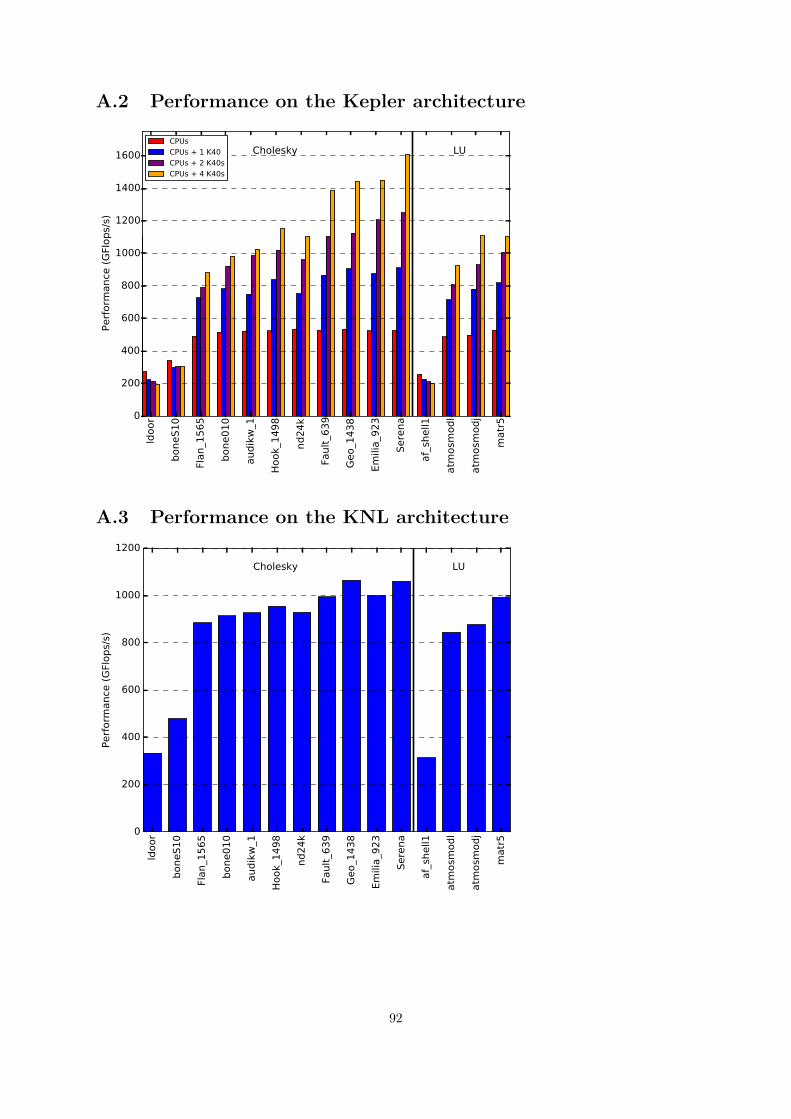
A.2 Performance on the Kepler architecture

ldoo

r

bone

S10

Flan

_156

5

bone

010

audi

kw_1

Hook

_149

8

nd24

k

Faul

t_63

9

Geo_

1438

Emili

a_92

3

Sere

na

af_s

hell1

atm

osm

odl

atm

osm

odj

mat

r5

0

200

400

600

800

1000

1200

1400

1600

Perfo

rman

ce (G

Flop

s/s)

Cholesky LUCPUsCPUs + 1 K40CPUs + 2 K40sCPUs + 4 K40s

A.3 Performance on the KNL architecture

ldoo

r

bone

S10

Flan

_156

5

bone

010

audi

kw_1

Hook

_149

8

nd24

k

Faul

t_63

9

Geo_

1438

Emilia

_923

Sere

na

af_s

hell1

atm

osm

odl

atm

osm

odj

mat

r5

0

200

400

600

800

1000

1200

Perfo

rman

ce (G

Flop

s/s)

Cholesky LU

92

Appendix B

Bibliography

[1] E. Agullo, J. Demmel, J. Dongarra, B. Hadri, J. Kurzak, J. Langou, H. Ltaief, P. Luszczek, andS. Tomov. Numerical linear algebra on emerging architectures: The PLASMA and MAGMAprojects. Journal of Physics: Conference Series, Vol. 180(1):012037, 2009. [Cited on pages 29and 30]

[2] E. Agullo, L. Giraud, A. Guermouche, A. Haidar, and J. Roman. Parallel algebraic domaindecomposition solver for the solution of augmented systems. Advances in Engineering Software,60(Supplement C):23 – 30, 2013. CIVIL-COMP: Parallel, Distributed, Grid and Cloud Computing.[Cited on pages 3 and 53]

[3] Emmanuel Agullo, Patrick R. Amestoy, Alfredo Buttari, Abdou Guermouche, Jean-YvesL’Excellent, and François-Henry Rouet. Robust Memory-Aware Mappings for Parallel MultifrontalFactorizations. SIAM Journal on Scientific Computing, 38(3), 2016. [Cited on page 81]

[4] P. Amestoy, I.S. Duff, S. Pralet, and C. Voemel. Adapting a parallel sparse direct solver to SMParchitectures. Parallel Computing, 29(11-12):1645–1668, 2003. [Cited on page 8]

[5] P. R. Amestoy, T. Davis, and I. S. Duff. An approximate minimum degree ordering algorithm.SIAM J. Matrix Anal. and Appl., 17:886–905, 1996. [Cited on pages 9 and 11]

[6] P. R. Amestoy, I. S. Duff, and J.-Y. L’Excellent. Multifrontal parallel distributed symmetric andunsymmetric solvers. Comput. Methods in Appl. Mech. Eng., 184:501–520, 2000. [Cited on pages7 and 52]

[7] P. R. Amestoy, I. S. Duff, J.-Y. L’Excellent, and X. S. Li. Analysis, tuning and comparison of twogeneral sparse solvers for distributed memory computers. ACM Trans. Math. Softw., 27(4):388–420,2001. [Cited on page 8]

[8] P. R. Amestoy, A. Guermouche, J.-Y. L’Excellent, and S. Pralet. Hybrid scheduling for the parallelsolution of linear systems. Parallel Computing, 32(2):136–156, 2006. [Cited on page 9]

[9] Patrick Amestoy, Cleve Ashcraft, Olivier Boiteau, Alfredo Buttari, Jean-Yves L’Excellent, andClement Weisbecker. Improving Multifrontal Methods by Means of Block Low-Rank Representa-tions. SIAM Journal on Scientific Computing, 37(3):A1451–A1474, 2015. [Cited on pages 72, 78,and 83]

[10] Patrick Amestoy, Alfredo Buttari, Jean-Yves L’Excellent, and Theo Mary. On the Complexityof the Block Low-Rank Multifrontal Factorization. Research Report RT–2016–03–FR, IRIT, May2016. [Cited on page 83]

[11] Patrick R Amestoy, Iain S Duff, Stephane Pralet, and Christof Vomel. Adapting a parallel sparsedirect solver to architectures with clusters of smps. Parallel Computing, 29(11):1645 – 1668, 2003.Parallel and distributed scientific and engineering computing. [Cited on page 43]

[12] A. Aminfar, S. Ambikasaran, and E. Darve. A fast block low-rank dense solver with applications tofinite-element matrices. Journal of Computational Physics, 304:170–188, 2016. [Cited on page 72]

93

[13] AmirHossein Aminfar and Eric Darve. A fast, memory efficient and robust sparse preconditionerbased on a multifrontal approach with applications to finite-element matrices. International Journalfor Numerical Methods in Engineering, 2016. [Cited on page 72]

[14] J Anton, C Ashcraft, and C Weisbecker. A Block Low-Rank Multithreaded Factorization for DenseBEM Operators. In SIAM Conference on Parallel Processing for Scientific Computing (SIAM PP2016), Paris, France, April 2016. [Cited on pages 72, 76, 78, and 83]

[15] Gabriel Antoniu, Luc Bougé, and Raymond Namyst. An efficient and transparent thread migrationscheme in the PM2 runtime system, pages 496–510. Springer Berlin Heidelberg, Berlin, Heidelberg,1999. [Cited on page 2]

[16] Joseph Antony, Pete P. Janes, and Alistair P. Rendell. Exploring thread and memory placement onNUMA architectures: Solaris and Linux, UltraSPARC/FirePlane and Opteron/HyperTransport.In HiPC, pages 338–352, 2006. [Cited on page 21]

[17] David L. Applegate, Robert E. Bixby, Vasek Chvatal, andWilliam J. Cook. The Traveling SalesmanProblem: A Computational Study (Princeton Series in Applied Mathematics). Princeton UniversityPress, Princeton, NJ, USA, 2007. [Cited on page 71]

[18] A. Ashcraft, S. C. Eisenstat, and J. W.-H. Liu. A fan-in algorithm for distributed sparse numericalfactorization. SIAM Journal on Scientific and Statistical Computing, 11:593–599, 1990. [Cited onpage 87]

[19] C. Ashcraft, S. C. Eisenstat, J. W.-H. Liu, and A. Sherman. A comparison of three column baseddistributed sparse factorization schemes. In Proc. Fifth SIAM Conf. on Parallel Processing forScientific Computing, 1991. [Cited on page 14]

[20] Cleve Ashcraft. The Fan-Both Family of Column-Based Distributed Cholesky Factorization Algo-rithms, pages 159–190. Springer New York, New York, NY, 1993. [Cited on page 16]

[21] Cédric Augonnet, Samuel Thibault, Raymond Namyst, and Pierre-André Wacrenier. StarPU: aunified platform for task scheduling on heterogeneous multicore architectures. Concurrency andComputation: Practice and Experience, 23(2), 2011. [Cited on pages 30 and 31]

[22] Maxime Barrault, Bruno Lathuilière, Pierre Ramet, and Jean Roman. Efficient Parallel Resolutionof The Simplified Transport Equations in Mixed-Dual Formulation. Journal of ComputationalPhysics, 230(5):2004–2020, 2011. [Cited on page 5]

[23] George Bosilca, Aurelien Bouteiller, Anthony Danalis, Mathieu Faverge, Azzam Haidar, ThomasHerault, Jakub Kurzak, Julien Langou, Pierre Lemarinier, Hatem Ltaief, Piotr Luszczek, AsimYarKhan, and Jack Dongarra. Flexible development of dense linear algebra algorithms on massivelyparallel architectures with DPLASMA. In 12th IEEE International Workshop on Parallel andDistributed Scientific and Engineering Computing (PDSEC’11), 2011. [Cited on pages 30 and 31]

[24] George Bosilca, Aurelien Bouteiller, Anthony Danalis, Thomas Hérault, Pierre Lemarinier, andJack Dongarra. DAGuE: A generic distributed DAG engine for High Performance Computing.Parallel Computing, 38(1-2), 2012. [Cited on page 30]

[25] Jacques Briat, Ilan Ginzburg, Marcelo Pasin, and Brigitte Plateau. Athapascan runtime: Efficiencyfor irregular problems, pages 591–600. Springer Berlin Heidelberg, Berlin, Heidelberg, 1997. [Citedon page 2]

[26] François Broquedis, Jérôme Clet-Ortega, Stéphanie Moreaud, Nathalie Furmento, Brice Goglin,Guillaume Mercier, Samuel Thibault, and Raymond Namyst. hwloc: A Generic Framework forManaging Hardware Affinities in HPC Applications. In Proceedings of the 18th Euromicro In-ternational Conference on Parallel, Distributed and Network-Based Processing (PDP2010), pages180–186, Pisa, Italia, February 2010. IEEE Computer Society Press. [Cited on page 30]

[27] A. Buttari. Fine-grained multithreading for the multifrontal QR factorization of sparse matrices,2013. To appear in SIAM SISC and APO technical report number RT-APO-11-6. [Cited on page 29]

94

[28] A. Buttari, J. Dongarra, J. Kurzak, J. Langou, P. Luszczek, and S. Tomov. The impact of multicoreon math software. In Proceedings of the 8th international conference on Applied parallel computing:state of the art in scientific computing, PARA’06, pages 1–10, Berlin, Heidelberg, 2007. Springer-Verlag. [Cited on page 29]

[29] Alfredo Buttari, Julien Langou, Jakub Kurzak, and Jack Dongarra. A class of parallel tiled linearalgebra algorithms for multicore architectures. Parallel Computing, 35(1):38–53, 2009. [Cited onpages 29, 30, and 33]

[30] Y. Campbell and T.A. Davis. Incomplete LU factorization: A multifrontal approach. Technicalreport, Technical Report TR-95-024, Computer and Information Sciences, Department Universityof Florida, Gainesville, FL, USA, October 1995. [Cited on page 44]

[31] A. Casadei. Optimizations of hybrid sparse linear solvers relying on Schur complement and domaindecomposition approaches. PhD thesis, LaBRI, Bordeaux University, Talence, France, October2015. [Cited on page 43]

[32] Astrid Casadei, Pierre Ramet, and Jean Roman. An improved recursive graph bipartitioningalgorithm for well balanced domain decomposition. In IEEE International Conference on HighPerformance Computing (HiPC 2014), pages 1–10, Goa, India, December 2014. [Cited on page 43]

[33] J. N. Chadwick and D. S. Bindel. An Efficient Solver for Sparse Linear Systems Based on Rank-Structured Cholesky Factorization. CoRR, abs/1507.05593, 2015. [Cited on page 72]

[34] Tony F. Chan and Panayot S. Vassilevski. A framework for block ilu factorizations using block-sizereduction. Mathematics of Computation, 64(209):129–156, 1995. [Cited on page 44]

[35] M. Chanaud. Conception d’un solveur haute performance de systèmes linéaires creux couplantdes méthodes multigrilles et directes pour la résolution des équations de Maxwell 3D en régimeharmonique discrétisées par éléments finis. PhD thesis, LaBRI, Bordeaux University, Talence,France, December 2009. [Cited on page 5]

[36] M. Chanaud, L. Giraud, D. Goudin, J. J. Pesqué, and J. Roman. A parallel full geometric multigridsolver for time harmonic maxwell problems. SIAM Journal on Scientific Computing, 36(2):C119–C138, 2014. [Cited on page 5]

[37] Andrew Chapman and Yousef Saad. Deflated and augmented krylov subspace techniques. Numer-ical Linear Algebra with Applications, 4(1):43–66, 1997. [Cited on page 45]

[38] P. Charrier and J. Roman. Algorithmique et calculs de complexité pour un solveur de type dissec-tions emboîtées. Numerische Mathematik, 55:463–476, 1989. [Cited on pages 10, 11, and 67]

[39] Michel Cosnard, Emmanuel Jeannot, and Tao Yang. Compact dag representation and its symbolicscheduling. Journal of Parallel and Distributed Computing, 64(8):921–935, 2004. [Cited on page 31]

[40] T. Davis. Direct Methods for Sparse Linear Systems. Society for Industrial and Applied Mathe-matics, 2006. [Cited on page 8]

[41] T. Davis. Multifrontal sparse qr factorization: Multicore, and gpu work in progress. In 15th SIAMConference on Parallel Processing for Scientific Computing, Savannah, USA, February 2012. [Citedon page 30]

[42] T. A. Davis. Algorithm 915, SuiteSparseQR: Multifrontal multithreaded rank-revealing sparse QRfactorization. ACM Trans. Math. Softw., 38(1):8, 2011. [Cited on page 29]

[43] T. A. Davis and Y. Hu. The University of Florida sparse matrix collection. ACM Trans. Math.Softw., 38(1):1:1–1:25, December 2011. [Cited on pages 33 and 78]

[44] Timothy A. Davis, Sivasankaran Rajamanickam, and Wissam M. Sid-Lakhdar. A survey of directmethods for sparse linear systems. Acta Numerica, 25:383–566, 2016. [Cited on page 2]

95

[45] R. Diekmann, R. Preis, F. Schlimbach, and C. Walshaw. Shape-optimized mesh partitioning andload balancing for parallel adaptive FEM. Parallel Computing, 26:1555–1581, 2000. [Cited onpage 57]

[46] I. S. Duff, A. M. Erisman, and J. K. Reid. Direct methods for sparse matrices. Oxford UniversityPress, London 1986. [Cited on pages 7 and 8]

[47] I. S. Duff and J. K. Reid. The multifrontal solution of indefinite sparse symmetric linear equations.ACM Transactions on Mathematical Software, 9:302–325, 1983. [Cited on page 7]

[48] M. Faverge. Ordonnancement hybride statique-dynamique en algèbre linéaire creuse pour de grandsclusters de machines NUMA et multi-coeurs. PhD thesis, LaBRI, Bordeaux University, Talence,France, December 2009. [Cited on page 19]

[49] Mathieu Faverge and Pierre Ramet. Dynamic Scheduling for sparse direct Solver on NUMA archi-tectures. In PARA’08, LNCS, Norway, 2008. [Cited on pages 19 and 29]

[50] J. Gaidamour. Conception d’un solveur linéaire creux parallèle hybride direct-itératif. PhD thesis,LaBRI, Bordeaux University, Talence, France, December 2009. [Cited on page 3]

[51] J. Gaidamour and P. Hénon. A parallel direct/iterative solver based on a Schur complementapproach. In IEEE 11th International Conference on Computational Science and Engineering,pages 98–105, Sao Paulo, Brésil, July 2008. [Cited on pages 3 and 53]

[52] A. George. Nested dissection of a regular finite element mesh. SIAM Journal on NumericalAnalysis, 10(2):345–363, 1973. [Cited on page 52]

[53] A. George, M. T. Heath, J. W.-H. Liu, and E. G.-Y. Ng. Sparse Cholesky factorization on a localmemory multiprocessor. SIAM Journal on Scientific and Statistical Computing, 9:327–340, 1988.[Cited on page 7]

[54] A. George and J. W.-H. Liu. Computer Solution of Large Sparse Positive Definite Systems.Prentice-Hall, Englewood Cliffs, NJ, 1981. [Cited on pages 7, 8, 9, and 68]

[55] A. George and D. R. McIntyre. On the application of the minimum degree algorithm to finiteelement systems. SIAM Journal on Numerical Analysis, 15(1):90–112, 1978. [Cited on page 70]

[56] T George, V Saxena, A Gupta, A Singh, and A R Choudhury. Multifrontal Factorization of SparseSPD Matrices on GPUs. 2011 IEEE International Parallel & Distributed Processing Symposium,pages 372–383, May 2011. [Cited on page 30]

[57] Pieter Ghysels, Xiaoye S. Li, François-Henry Rouet, Samuel Williams, and Artem Napov. An Effi-cient Multicore Implementation of a Novel HSS-Structured Multifrontal Solver Using RandomizedSampling. SIAM Journal on Scientific Computing, 38(5):S358–S384, 2016. [Cited on page 72]

[58] L. Giraud, A. Haidar, and Y. Saad. Sparse approximations of the Schur complement for parallelalgebraic hybrid linear solvers in 3D. Rapport de recherche RR-7237, INRIA, March 2010. [Citedon page 53]

[59] D. Goudin, P. Hénon, M. Mandallena, K. Mer, F. Pellegrini, P. Ramet, J. Roman, and J.-J. Pesqué.Outils numériques parallèles pour la résolution de très grands problèmes d’électromagnétisme. InSéminaire sur l’Algorithmique Numérique Appliquée aux Problèmes Industriels, Calais, France,May 2003. [Cited on page 8]

[60] D. Goudin, P. Hénon, F. Pellegrini, P. Ramet, J. Roman, and J.-J. Pesqué. Parallel sparse linearalgebra and application to structural mechanics. Numerical Algorithms, Baltzer Science Publisher,24:371–391, 2000. [Cited on page 8]

[61] L. Grasedyck, R. Kriemann, and S. Le Borne. Parallel black box H-LU preconditioning for ellipticboundary value problems. Computing and Visualization in Science, 11(4-6):273–291, 2008. [Citedon page 72]

96

[62] Lars Grasedyck, Wolfgang Hackbusch, and Ronald Kriemann. Performance of H-LU precondition-ing for sparse matrices. Computational methods in applied mathematics, 8(4):336–349, 2008. [Citedon page 72]

[63] L. Grigori, J. A. Demmel, and X. S. Li. Parallel Symbolic Factorization for Sparse LU with StaticPivoting. SIAM J. Sci. Comput., 29(3):1289–1314, 2007. [Cited on page 52]

[64] Anshul Gupta. Recent progress in general sparse direct solvers. In Lecture Notes in ComputerScience, volume 2073, pages 823–840, 2001. [Cited on page 43]

[65] W. Hackbusch. Hierarchical Matrices: Algorithms and Analysis, volume 49. Springer Series inComputational Mathematics, 2015. [Cited on pages 72 and 83]

[66] R. W. Hamming. Error Detecting and Error Correcting Codes. Bell System Technical Journal,26(2):147–160, 1950. [Cited on page 70]

[67] M. T. Heath, E. G.-Y. Ng, and B. W. Peyton. Parallel algorithms for sparse linear systems. SIAMReview, 33:420–460, 1991. [Cited on page 7]

[68] B. Hendrickson and R. Leland. A multi-level algorithm for partitioning graphs. In Supercomputing,1995. Proceedings of the IEEE/ACM SC95 Conference, pages 28–28, 1995. [Cited on page 53]

[69] B. Hendrickson and E. Rothberg. Improving the run time and quality of nested dissection ordering.SIAM Journal on Scientific Computing, 20(2):468–489, 1998. [Cited on page 53]

[70] Bruce Hendrickson and Tamara G. Kolda. Graph Partitioning Models for Parallel Computing.Parallel Computing, 26(12):1519–1534, 2000. [Cited on page 52]

[71] Bruce Hendrickson and Robert Leland. An improved spectral graph partitioning algorithm formapping parallel computations. SIAM J. Sci. Comput., 16(2):452–469, March 1995. [Cited onpage 9]

[72] P. Hénon. Distribution des Données et Régulation Statique des Calculs et des Communicationspour la Résolution de Grands Systèmes Linéaires Creux par Méthode Directe. PhD thesis, LaBRI,University Bordeaux 1, Talence, France, November 2001. [Cited on pages 11 and 14]

[73] P. Hénon, P. Ramet, and J. Roman. A Mapping and Scheduling Algorithm for Parallel SparseFan-In Numerical Factorization. In Proceedings of EuroPAR’99, number 1685 in Lecture Notes inComputer Science, pages 1059–1067. Springer Verlag, September 1999. [Cited on page 14]

[74] P. Hénon, P. Ramet, and J. Roman. PaStiX: A Parallel Sparse Direct Solver Based on a StaticScheduling for Mixed 1D/2D Block Distributions. In Proceedings of Irregular’2000, number 1800in Lecture Notes in Computer Science, pages 519–525. Springer Verlag, May 2000. [Cited on pages7, 8, 12, 14, 22, and 24]

[75] P. Hénon, P. Ramet, and J. Roman. PaStiX: A High-Performance Parallel Direct Solver for SparseSymmetric Definite Systems. Parallel Computing, 28(2):301–321, January 2002. [Cited on pages7, 8, 9, 10, 11, 14, 22, 43, 52, and 72]

[76] P. Hénon, P. Ramet, and J. Roman. Efficient algorithms for direct resolution of large sparse systemon clusters of SMP nodes. In SIAM Conference on Applied Linear Algebra, Williamsburg, Virginie,USA, July 2003. [Cited on pages 8, 11, and 43]

[77] P. Hénon, P. Ramet, and J. Roman. On finding approximate supernodes for an efficient ILU(k)factorization. Parallel Computing, 34:345–362, 2008. [Cited on pages 33 and 43]

[78] P. Hénon and Y. Saad. A parallel multistage ILU factorization based on a hierarchical graphdecomposition. SIAM Journal on Scientific Computing, 28(6):2266–2293, 2006. [Cited on page 3]

[79] Kenneth L Ho and Lexing Ying. Hierarchical interpolative factorization for elliptic operators:differential equations. Communications on Pure and Applied Mathematics, 2015. [Cited on page 72]

97

[80] Jonathan D. Hogg, John K. Reid, and Jennifer A. Scott. Design of a multicore sparse Choleskyfactorization using dags. SIAM Journal on Scientific Computing, 32(6):3627–3649, 2010. [Citedon pages 4 and 29]

[81] G. Huysmans, Stanislas Pamela, Emiel Van Der Plas, and Pierre Ramet. Non-linear MHD simu-lations of edge localized modes (ELMs). Plasma Physics, 51(12):124012, 2009. [Cited on page 5]

[82] David Hysom and Alex Pothen. A scalable parallel algorithm for incomplete factor preconditioning.SIAM Journal on Scientific Computing, 22(6):2194–2215, 2001. [Cited on pages 44 and 45]

[83] F. D. Igual, E. Chan, E. S. Quintana-Ortí, G. Quintana-Ortí, R. A. van de Geijn, and F. G. VanZee. The FLAME approach: From dense linear algebra algorithms to high-performance multi-accelerator implementations. J. Parallel Distrib. Comput., 72(9):1134–1143, 2012. [Cited onpage 30]

[84] David S. Johnson and Lyle A. Mcgeoch. The Traveling Salesman Problem: A Case Study in LocalOptimization, pages 215–310. Chichester, UK, 1997. [Cited on page 71]

[85] M. Joshi, G. Karypis, V. Kumar, A. Gupta, and F. Gustavson. PSPASES : Scalable Parallel DirectSolver Library for Sparse Symmetric Positive Definite Linear Systems. Technical report, Universityof Minnesota and IBM Thomas J. Watson Research Center, May 1999. [Cited on page 8]

[86] G. Karypis and V. Kumar. A fast and high quality multilevel scheme for partitioning irregulargraphs. SIAM Journal on Scientific Computing, 20(1):359–392, 1998. [Cited on page 53]

[87] G. Karypis and V. Kumar. MeTiS – A Software Package for Partitioning Unstructured Graphs,Partitioning Meshes, and Computing Fill-Reducing Orderings of Sparse Matrices – Version 4.0.University of Minnesota, September 1998. [Cited on pages 8, 9, 10, and 52]

[88] G. Karypis and V. Kumar. Multilevel k-way partitioning scheme for irregular graphs. Journal ofParallel and Distributed Computing, 48:96–129, 1998. [Cited on page 53]

[89] George Karypis and Vipin Kumar. Parallel threshold-based ilu factorization. In Proceedings of the1997 ACM/IEEE Conference on Supercomputing, SC ’97, pages 1–24, New York, NY, USA, 1997.ACM. [Cited on page 44]

[90] O. Kaya and B. Uçar. Scalable sparse tensor decompositions in distributed memory systems. InProceedings of the International Conference for High Performance Computing, Networking, Storageand Analysis, pages 77:1–77:11. ACM, 2015. [Cited on page 89]

[91] O. Kaya and B. Uçar. High performance parallel algorithms for the tucker decomposition of sparsetensors. In 45th International Conference on Parallel Processing (ICPP ’16), pages 103–112, 2016.[Cited on page 89]

[92] Kevin Barker and Kei Davis and Adolfy Hoisie and Darren Kerbyson and Michael Lang and ScottPakin and José Carlos Sancho. Experiences in Scaling Scientific Applications on Current-generationQuad-core Processors. In LSPP’08 held in conjunction with IPDPS, Miami, Florida, USA, April2008. [Cited on page 21]

[93] Ronald Kriemann. H-LU factorization on many-core systems. Computing and Visualization inScience, 16(3):105–117, 2013. [Cited on page 72]

[94] Jakub Kurzak, Stanimire Tomov, and Jack Dongarra. Autotuning GEMM Kernels for the FermiGPU. IEEE Transactions on Parallel and Distributed Systems, 23(11):2045–2057, 2012. [Cited onpage 38]

[95] X. Lacoste. Scheduling and memory optimizations for sparse direct solver on multi-core/multi-gpucluster systems. PhD thesis, Université Bordeaux, Talence, France, February 2015. [Cited on pages5, 19, and 78]

98

[96] Xavier Lacoste, Mathieu Faverge, Pierre Ramet, Samuel Thibault, and George Bosilca. TakingAdvantage of Hybrid Systems for Sparse Direct Solvers via Task-Based Runtimes. In ParallelDistributed Processing Symposium Workshops (IPDPSW), 2014 IEEE International, pages 29–38,Phoenix, United States, May 2014. IEEE. [Cited on page 19]

[97] B. Lathuilière. Méthode de décomposition de domaine pour les équations du transport simplifié enneutronique. PhD thesis, LaBRI, Bordeaux University, Talence, France, January 2010. [Cited onpage 5]

[98] X. S. Li. Evaluation of sparse LU factorization and triangular solution on multicore platforms. InJ. M. Laginha M. Palma, P. Amestoy, M. J. Daydé, M. Mattoso, and J. Correia Lopes, editors,VECPAR, volume 5336 of Lecture Notes in Computer Science, pages 287–300. Springer, 2008.[Cited on page 29]

[99] X. S. Li and J. W. Demmel. A scalable sparse direct solver using static pivoting. In Proceedings ofthe Ninth SIAM Conference on Parallel Processing for Scientific Computing, San Antonio, Texas,March 22-24, 1999. [Cited on pages 8 and 43]

[100] R. J. Lipton, D. J. Rose, and R. E. Tarjan. Generalized nested dissection. SIAM Journal onNumerical Analysis, 16(2), 1979. [Cited on pages 9, 52, and 53]

[101] R. J. Lipton and R. E. Tarjan. A separator theorem for planar graphs. SIAM Journal on AppliedMathematics, 36:177–189, 1979. [Cited on pages 78 and 84]

[102] J. W.-H. Liu. Modification of the minimum-degree algorithm by multiple elimination. ACM Trans.Math. Software, 11(2):141–153, 1985. [Cited on page 8]

[103] J. W.-H. Liu. The role of elimination trees in sparse factorization. SIAM J. Matrix Anal. Appl.,11:134–172, 1990. [Cited on page 9]

[104] Joseph W. H. Liu, Esmond G. Ng, and Barry W. Peyton. On finding supernodes for sparse matrixcomputations. SIAM Journal on Matrix Analysis and Applications, 14(1):242–252, 1993. [Citedon page 10]

[105] R. F. Lucas, G. Wagenbreth, D. M. Davis, and R. Grimes. Multifrontal computations on GPUsand their multi-core hosts. In Proceedings of the 9th international conference on High performancecomputing for computational science, VECPAR’10, pages 71–82, Berlin, Heidelberg, 2011. Springer-Verlag. [Cited on page 30]

[106] María J. Martín, Inmaculada Pardines, and Francisco F. Rivera. Scheduling of algorithms basedon elimination trees on NUMA systems. In EuroPar’99, volume 1685 of Lecture Notes in ComputerScience, pages 1068–1072, Toulouse, France, 1999. [Cited on page 22]

[107] Henning Meyerhenke, Burkhard Monien, and Thomas Sauerwald. A new diffusion-based multilevelalgorithm for computing graph partitions. J. Parallel Distrib. Comput., 69(9):750–761, September2009. [Cited on page 57]

[108] G. L. Miller, S.-H. Teng, and S. A. Vavasis. A unified geometric approach to graph separators. InProc. 31st Annual Symposium on Foundations of Computer Science, pages 538–547, 1991. [Citedon page 52]

[109] G. L. Miller and S. A. Vavasis. Density graphs and separators. In Second Annual ACM-SIAMSymposium on Discrete Algorithms, pages 331–336, 1991. [Cited on page 52]

[110] M. Magolu monga Made and H.A. van der Vorst. A generalized domain decomposition paradigmfor parallel incomplete lu factorization preconditionings. Future Generation Computer Systems,17(8):925 – 932, 2001. High Performance Computing and Networking. [Cited on page 43]

[111] S. Moustafa. Massively Parallel Cartesian Discrete Ordinates Method for Neutron Transport Sim-ulation. PhD thesis, LaBRI, Bordeaux University, Talence, France, December 2015. [Cited onpage 5]

99

[112] Salli Moustafa, Ivan Dutka Malen, Laurent Plagne, Angélique Ponçot, and Pierre Ramet. SharedMemory Parallelism for 3D Cartesian Discrete Ordinates Solver. Annals of Nuclear Energy, pages1–10, September 2014. [Cited on page 5]

[113] Rajib Nath, Stanimire Tomov, and Jack Dongarra. An improved MAGMA GEMM for Fermigraphics processing units. International Journal of High Performance Computing Applications,24(4):511–515, 2010. [Cited on page 38]

[114] CUDA Nvidia. Cublas library. NVIDIA Corporation, Santa Clara, California, 15, 2008. [Cited onpage 38]

[115] F. Pellegrini and J. Roman. Scotch: A software package for static mapping by dual recursivebipartitioning of process and architecture graphs. In High-Performance Computing and Networking,volume 1067 of Lecture Notes in Computer Science, pages 493–498. Springer, 1996. [Cited onpage 52]

[116] F. Pellegrini and J. Roman. Sparse matrix ordering with scotch. In Proceedings of HPCN’97,Vienna, LNCS 1225, pages 370–378, April 1997. [Cited on pages 9 and 11]

[117] F. Pellegrini, J. Roman, and P. Amestoy. Hybridizing nested dissection and halo approximateminimum degree for efficient sparse matrix ordering. Concurrency: Practice and Experience, 12:69–84, 2000. Preliminary version published in Proceedings of Irregular’99, LNCS 1586, 986–995. [Citedon pages 9 and 11]

[118] Francois Pellegrini. Scotch and libScotch 5.1 User’s Guide, August 2008. [Cited on pages 10 and 78]

[119] G. Pichon, E. Darve, M. Faverge, P. Ramet, and J. Roman. Sparse supernodal solver using blocklow-rank compression. In 2017 IEEE International Parallel and Distributed Processing SymposiumWorkshops (IPDPSW), pages 1138–1147, May 2017. [Cited on page 67]

[120] Gregoire Pichon, Mathieu Faverge, Pierre Ramet, and Jean Roman. Reordering strategy for block-ing optimization in sparse linear solvers. SIAM Journal on Matrix Analysis and Applications,38(1):226–248, 2017. [Cited on page 67]

[121] A. Pothen and C. Sun. A mapping algorithm for parallel sparse Cholesky factorization. SIAM J.Sci. Comput., 14(5):1253–1257, September 1993. [Cited on pages 7 and 15]

[122] Hadi Pouransari, Pieter Coulier, and Eric Darve. Fast hierarchical solvers for sparse matricesusing extended sparsification and low-rank approximation. arXiv preprint arXiv:1510.07363v3,2015. [Cited on page 72]

[123] G. Quintana-Ortí, E. S. Quintana-Ortí, R. A. van de Geijn, F. G. Van Zee, and E. Chan. Program-ming matrix algorithms-by-blocks for thread-level parallelism. ACM Trans. Math. Softw., 36(3),2009. [Cited on page 30]

[124] Padma Raghavan, Keita Teranishi, and Esmond G. Ng. A latency tolerant hybrid sparse solverusing incomplete cholesky factorization. Numerical Linear Algebra with Applications, 10(5-6):541–560, 2003. [Cited on page 43]

[125] S. Rajamanickam, E.G. Boman, and M.A. Heroux. ShyLU: A hybrid-hybrid solver for multicoreplatforms. In Parallel Distributed Processing Symposium (IPDPS), 2012 IEEE 26th International,pages 631–643, May 2012. [Cited on page 53]

[126] Donald J. Rose, R. Endre Tarjan, and George S. Lueker. Algorithmic aspects of vertex eliminationon graphs. SIAM Journal on Computing, 5(2):266–283, 1976. [Cited on page 44]

[127] E. Rothberg and A. Gupta. An efficient block-oriented approach to parallel sparse Cholesky fac-torization. SIAM J. Sci. Comput., 15(6):1413–1439, November 1994. [Cited on page 7]

[128] Y. Saad. ILUT: A dual threshold incomplete lu factorization. Numerical Linear Algebra withApplications, 1(4):387–402, 1994. [Cited on page 44]

100

[129] Y. Saad. Iterative Methods for Sparse Linear Systems. Society for Industrial and Applied Mathe-matics, second edition, 2003. [Cited on pages 43 and 44]

[130] O. Schenk and K. Gärtner. Solving unsymmetric sparse systems of linear equations with pardiso.Future Gener. Comput. Syst., 20(3):475–487, 2004. [Cited on page 29]

[131] W. M. Sid-Lakhdar. Scaling the solution of large sparse linear systems using multifrontal methodson hybrid shared-distributed memory architectures. PhD thesis, Ecole Normale Supérieure de Lyon,December 2014. [Cited on page 70]

[132] Shaden Smith and George Karypis. Accelerating the tucker decomposition with compressed sparsetensors. In European Conference on Parallel Processing. Springer, 2017. [Cited on page 89]

[133] Shaden Smith, Jongsoo Park, and George Karypis. Sparse tensor factorization on many-core pro-cessors with high-bandwidth memory. 31st IEEE International Parallel & Distributed ProcessingSymposium (IPDPS’17), 2017. [Cited on page 89]

[134] STFC. HSL. A collection of Fortran codes for large scale scientific computation. http://www.hsl.rl.ac.uk/. [Cited on pages 4 and 70]

[135] Daria A Sushnikova and Ivan V Oseledets. “Compress and eliminate” solver for symmetric positivedefinite sparse matrices. arXiv preprint arXiv:1603.09133v3, 2016. [Cited on page 72]

[136] Guangming Tan, Linchuan Li, Sean Triechle, Everett Phillips, Yungang Bao, and Ninghui Sun.Fast implementation of dgemm on fermi gpu. In Proceedings of 2011 International Conference forHigh Performance Computing, Networking, Storage and Analysis, SC ’11, pages 35:1–35:11, NewYork, NY, USA, 2011. ACM. [Cited on page 38]

[137] Rajeev Thakur and William Gropp. Test suite for evaluating performance of MPI implementationsthat support MPI_THREAD_MULTIPLE. In EuroPVM/MPI, volume 4757 of Lecture Notes inComputer Science, pages 46–55, 2007. [Cited on page 23]

[138] Francois Trahay, Alexandre Denis, Olivier Aumage, and Raymond Namyst. Improving reactivityand communication overlap in MPI using a generic I/O manager. In EuroPVM/MPI, volume 4757of Lecture Notes in Computer Science, pages 170–177, 2007. [Cited on page 22]

[139] Field G Van Zee, Ernie Chan, Robert A Van de Geijn, Enrique S Quintana-Orti, and GregorioQuintana-Orti. The LibFlame library for dense matrix computations. Computing in science &engineering, 11(6):56–63, 2009. [Cited on page 30]

[140] Vasily Volkov and James W. Demmel. Benchmarking GPUs to tune dense linear algebra. InProceedings of the 2008 ACM/IEEE conference on Supercomputing, SC ’08, pages 31:1–31:11,Piscataway, NJ, USA, 2008. IEEE Press. [Cited on pages 33 and 38]

[141] Shen Wang, Xiaoye S. Li, François-Henry Rouet, Jianlin Xia, and Maarten V. De Hoop. A ParallelGeometric Multifrontal Solver Using Hierarchically Semiseparable Structure. ACM Trans. Math.Softw., 42(3):21:1–21:21, May 2016. [Cited on page 72]

[142] James W. Watts III. A conjugate gradient-truncated direct method for the iterative solution ofthe reservoir simulation pressure equation. June 1981. [Cited on page 44]

[143] Jianlin Xia, Shivkumar Chandrasekaran, Ming Gu, and Xiaoye S. Li. Superfast multifrontal methodfor large structured linear systems of equations. SIAM Journal on Matrix Analysis and Applica-tions, 31(3):1382–1411, 2010. [Cited on page 72]

[144] Ichitaro Yamazaki and Xiaoye S. Li. On techniques to improve robustness and scalability ofa parallel hybrid linear solver. In High Performance Computing for Computational Science –VECPAR 2010, volume 6449 of Lecture Notes in Computer Science, pages 421–434. Springer,2011. [Cited on page 53]

[145] Ichitaro Yamazaki, Stanimire Tomov, and Jack Dongarra. One-sided Dense Matrix Factorizationson a Multicore with Multiple GPU Accelerators. Procedia Computer Science, 9(Complete):37–46,2012. [Cited on page 37]

101

[146] Kai Yang, Hadi Pouransari, and Eric Darve. Sparse hierarchical solvers with guaranteed conver-gence. arXiv preprint arXiv:1611.03189, 2016. [Cited on page 72]

[147] A. YarKhan. Dynamic Task Execution on Shared and Distributed Memory Architectures. PhDthesis, Innovative Computing Laboratory, University of Tennessee, dec 2012. [Cited on page 30]

[148] C D Yu, W Wang, and D Pierce. A CPU-GPU Hybrid Approach for the Unsymmetric MultifrontalMethod. Parallel Computing, 37(12):759–770, October 2011. [Cited on page 30]

102