1

Here are additional dictionary definitions of data. Notice the third definition, it restricts data to digital data.

2

In a broad sense, data doesn’t have to be digital. Analog data is data represented in continuous form. We are not trying to get into an argument whether matter is continuous or discrete. Quantum physics, Heisenberg’s uncertainty principle, and the dual wave/particle aspect of light—you learn about them in a different class.

3

Here is an example of continuous data. These color photographs were taken 100 years ago by Russia’s photographer to the tsar. Are they data? Of course, they provide a lot of and important information about those times. Are they digital? No. No pixels yet. It’s even before Kodak. Notice that they are color photographs. How were they taken? Prokudin took three slides, one with a red filter in front of the lens, one with a green, and one with a blue filter. Then put the three slides on top of each other, place a bright (white) light behind them, and you project in color. RGB existed before color TVs and pixels. Why does the river look like it is covered with a film of oil? Pollution? No, of course not. Think of how the slides were taken.

4

Here are additional examples. Music has of course been recorded with analog devices.

5

Electronics was also analog at the beginning.

6

What are the shortcomings of analog data? Storage is inefficient—big volume, small amount of data. Modifying the level of detail is not easy. Consider Prokudin’s photos. How could he have obtained a smaller photo from a large photo? He probably would have needed to project the large photo, then take a picture of the projection using smaller film, etc. Modifying data level of detail is essential, because not all applications need the data at the highest level of detail all the time. Transmitting analog data is also inefficient—a little bit of analog data consumes a lot of bandwidth. A few years ago, TV broadcasts switched from analog to digital. Why? In order to be able to have more channels. Replication is another huge challenge. Every time you copy analog data quality goes down. For example recording from a VCR tape to another VCR tape lower quality. That’s why you need to always use the master tape as source. This slows down replication. Instead of being able to replicate from the ever increasing number of copies, you have to always go back to the master tape.

7

To overcome these disadvantages, the world moved to digital data. Digital data is data represented in discrete form, using numbers. For example, for digital music, I encode with a number what the music sounds like every millisecond. Since a millisecond is a very short time interval, all these values are a good approximation of the overall music. Of course, one immediate challenge is that the real world is not discrete. So in order to acquire digital data, one needs to digitize the input signal. Analog to digital conversion or digitization is essential for obtaining digital data.

8

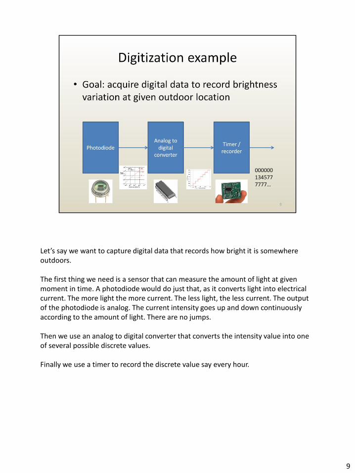
Let’s say we want to capture digital data that records how bright it is somewhere outdoors. The first thing we need is a sensor that can measure the amount of light at given moment in time. A photodiode would do just that, as it converts light into electrical current. The more light the more current. The less light, the less current. The output of the photodiode is analog. The current intensity goes up and down continuously according to the amount of light. There are no jumps. Then we use an analog to digital converter that converts the intensity value into one of several possible discrete values. Finally we use a timer to record the discrete value say every hour.

9

Here is the resulting digital data over 24h. Each row represents 24h worth of data. Since we digitize every hour, there are 24 columns. There are 8 possible brightness levels: 0 through 7.

10

The first row could be a summer day in Indiana, the second row a winter day in Indiana, the third row a summer day in Alaska, and finally a winter day at the North Pole.

11

Here are additional digitization examples. The CD and the CD player popularized digital music. The mic is the photodiode from the previous example. Then everything else is the same. A digital camera measures light intensity over discrete rectangular regions, called pixels. The result is a digital image, or a matrix of numbers, one number for each pixel. Scanners work similarly, they are digital cameras specialized for flat (paper) documents.

12

An incredible advantage of digital data is that it can be replicated endlessly without loss of quality. Any copy is as good as the original and can be used to make additional copies. As you know, this created huge problems for the recording industry.

13

Another advantage is that one can easily control the level of detail. Let’s say we only want to know the brightness every four hours. That can be easily done by averaging four consecutive numbers from the original data.

14

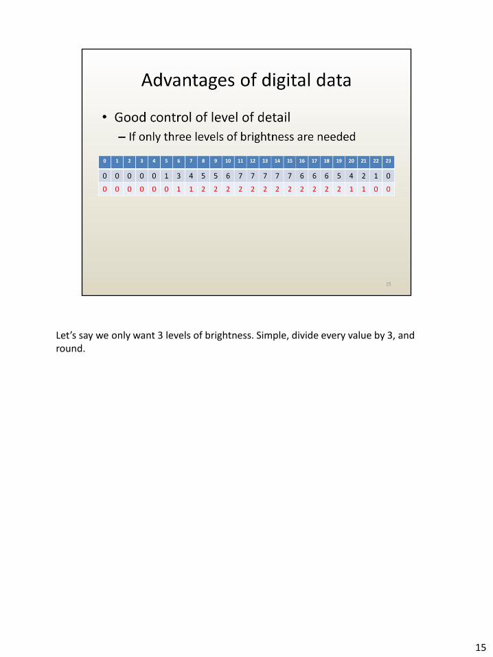
Let’s say we only want 3 levels of brightness. Simple, divide every value by 3, and round.

15

Digital data has challenges of its own. A fundamental limitation is that digital data has limited precision. Digital data provides an approximation. No matter how densely one samples (i.e. digitizes) and how many discrete levels are used, the digital data will not capture the full complexity of what it records. A second challenge is that computing hardware becomes very expensive for digital data with many discrete levels. For example in base 10, the computer needs to distinguish between 10 digits. The solution to this problem is to use the simples base possible, base 2.

16

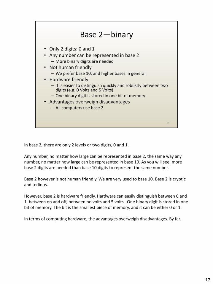
In base 2, there are only 2 levels or two digits, 0 and 1. Any number, no matter how large can be represented in base 2, the same way any number, no matter how large can be represented in base 10. As you will see, more base 2 digits are needed than base 10 digits to represent the same number. Base 2 however is not human friendly. We are very used to base 10. Base 2 is cryptic and tedious. However, base 2 is hardware friendly. Hardware can easily distinguish between 0 and 1, between on and off, between no volts and 5 volts. One binary digit is stored in one bit of memory. The bit is the smallest piece of memory, and it can be either 0 or 1. In terms of computing hardware, the advantages overweigh disadvantages. By far.

17

When one counts in base 2, one uses boxes of size power of 2. In base 10 the boxes are of size power of 10: 1, 10, 100, 1000. In base 2, the boxes are of size 1, 2, 4, 8, 16, etc. Counting is done with a “greedy approach”: always use the biggest box that you can fill. So if we want to count these 7 dots in base 2, we first find the largest box we can fill. Can we use an 8 box? No, because it wouldn’t be full. A 4-box? Yes. So 1 4-box. That’s the 1 from the left. We are left with counting the remaining 3 dots: 1 box of size 2, and then 1 box of size 1, which gives us the other two ones. The subindex indicates the base. 7 in base 10 is 111 in base 2. Again: 111 in base 2 means 1 box of 4 + 1 box of 2 + 1 box of 1, total 7.

18

Here is another example. Counting 9 dots in base 2. The boxes are of size 1, 2, 4, 8, 16, 32, … 16 wouldn’t be full. So 1 8-box. 1 dots is left over. Can we fill a 4-box? No, so 0 4-boxes. A 2-box? No, so 0 2-boxes. Finally we have 1 1-box. So that 1, 0, 0, 1. It’s just like in base 100. Let’s say there were one three hundred and one dots. How many boxes of 100? 3. Of 10? 0. Of 1? 1. So that’s 301.

19

20

21

OK, let’s try base 8 now. 8 digits, from 0 to 7. The boxes are of size 1, 8, 64, etc.—the powers of 8. Let’s count 13 dots. No 64-box, obviously. 1 8-box. 5 1-boxes. So that’s 1, 5 in base 8.

22

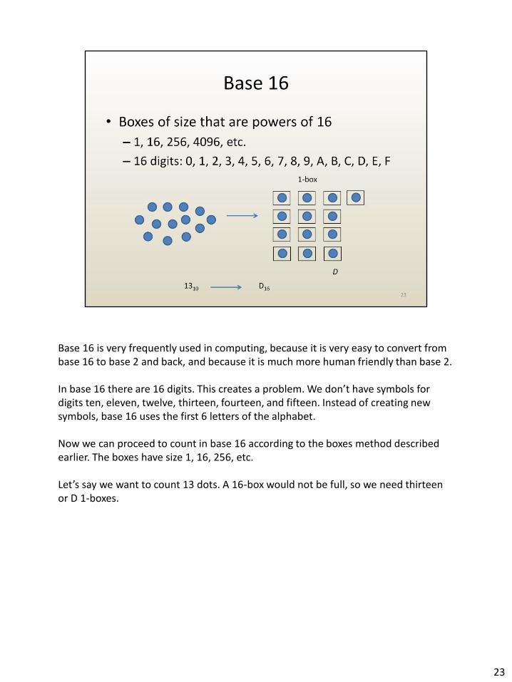
Base 16 is very frequently used in computing, because it is very easy to convert from base 16 to base 2 and back, and because it is much more human friendly than base 2. In base 16 there are 16 digits. This creates a problem. We don’t have symbols for digits ten, eleven, twelve, thirteen, fourteen, and fifteen. Instead of creating new symbols, base 16 uses the first 6 letters of the alphabet. Now we can proceed to count in base 16 according to the boxes method described earlier. The boxes have size 1, 16, 256, etc. Let’s say we want to count 13 dots. A 16-box would not be full, so we need thirteen or D 1-boxes.

23

We said base 16’s raison d’etre is to make base 2 (which is used by computing HW and cannot be avoided) more human friendly, while providing a simple conversion back and forth (i.e. from base 2 to base 16 and back). The golden rule when converting base 2 into base 16 and back is to know that 4 binary digits correspond to one hexadecimal (i.e. base 16) digit. Then, if you know the binary representation of each hexadecimal digit, you can convert any number of any size very quickly. The top two tables provide the base 2 representation of each of the 16 base 16 digits.

24

25

All data is encoded in binary, but there are many types of data. Characters are used to encode textual data. A character corresponds to a letter, to a symbol (e.g. $, %, ^, &), to a digit, etc. There are fewer than 256 characters, so 8 bits are sufficient to encode a character. In other words, one can count from 0 to 255 using 8 bits. 255 corresponds to eight 1s or 1111 1111. This means that there are 256 unique binary numbers with 8 bits. Each character can be assigned a unique 8 bit code. A group of 8 bits are called a byte.

26

Let’s take a moment to clarify bits and bytes, kilo, Mega and Giga. The first thing to remember is that in computer science, 1 Mega is 1,024 kilo, 1 Giga is 1,024 Mega, as opposed to 1,000. The second thing to remember is that a byte is abbreviated with an upper case B and a bit is abbreviated with a lower case b. A byte is 8 bits. A byte is not the same as a bit. Consequently when you mean byte, write an upper case B.

27

28

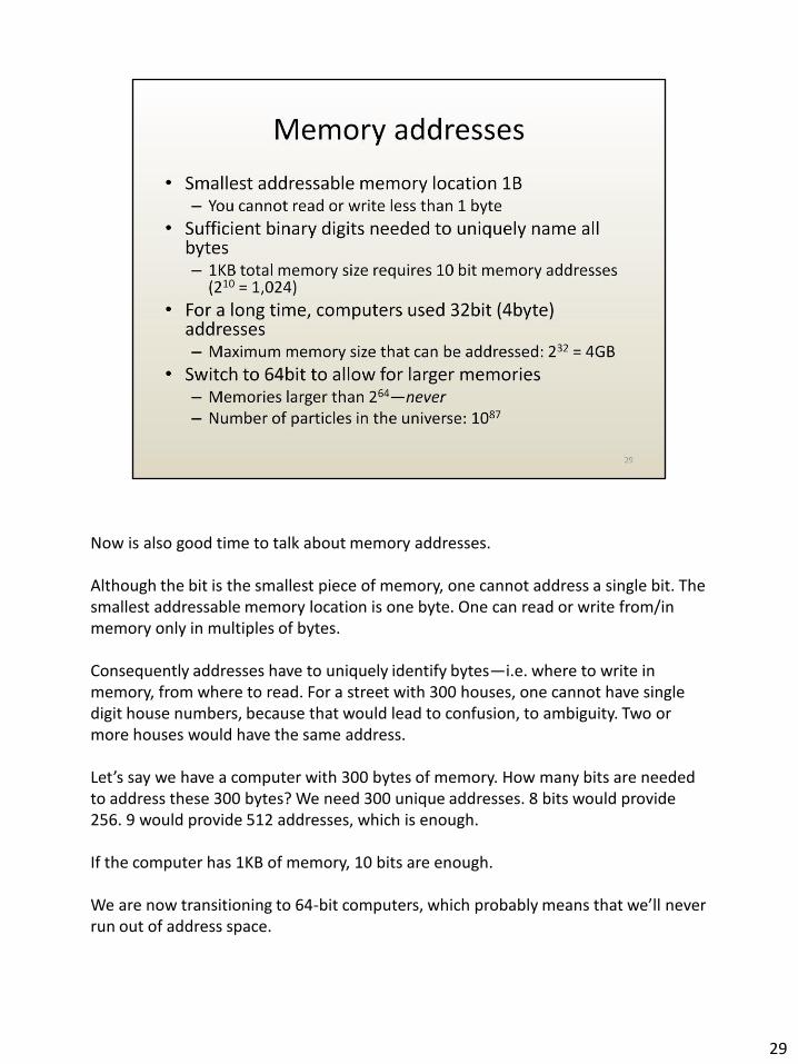
Now is also good time to talk about memory addresses. Although the bit is the smallest piece of memory, one cannot address a single bit. The smallest addressable memory location is one byte. One can read or write from/in memory only in multiples of bytes. Consequently addresses have to uniquely identify bytes—i.e. where to write in memory, from where to read. For a street with 300 houses, one cannot have single digit house numbers, because that would lead to confusion, to ambiguity. Two or more houses would have the same address. Let’s say we have a computer with 300 bytes of memory. How many bits are needed to address these 300 bytes? We need 300 unique addresses. 8 bits would provide 256. 9 would provide 512 addresses, which is enough. If the computer has 1KB of memory, 10 bits are enough. We are now transitioning to 64-bit computers, which probably means that we’ll never run out of address space.

29

Back to data types. In addition to characters for encoding textual data, there is also the need to encode numbers. Integers are used to encode numbers w/o a fractional component. If we encode unsigned integers with 4 bytes, the largest number that can be represented is 232-1, which is over 4 billion. Let’s write it in base 16. One byte corresponds to 8 bits, or 2 hexadecimal digits. Consequently 4 bytes correspond to 8 hexadecimal digits. The largest 4-byte unsigned integer in hexadecimal is FF FF FF FF (i.e. 32 ones in base 2, or 1111 1111 1111 1111 1111 1111 1111 1111 ).

30

To encode real numbers, one has to allow for a fractional component. When a “fixed point” encoding is used, there is no exponent.

31

A more flexible representation of real numbers allows for an exponent.

32

No matter how many bits are allocated to numbers, after long chains of arithmetic operations, the precision of the result will be less than that of the input operands.

33

So far we have discussed simple data types: characters, integer numbers, real numbers. These basic types can be combined to form compound data types. Multiple characters form a string which allows text processing. Multiple floating point numbers form vectors which are used for example in physics simulations. Strings, vectors, dates, and so on can be combined to form a complete medical record of a patient.

34

Here is an example of a compound data type used for a computer aided design (CAD) application. At the top level, the data type is called Car.

35

The car has three components.

36

Components have sub-components.

37

Sub-components have sub-sub-components and so on.

38

Compound data types make complexity tractable by abstracting away (i.e. hiding) details. Hierarchical modeling is a fundamental paradigm in computer science. Creativity: “I want to develop a more aerodynamic shape. I don’t need and shouldn’t see the engine”. Repair: “The engine won’t start. Is the fuel system OK? Yes it is, check, I am not going to worry about it anymore. Is the ignition system OK? No. Is the battery OK? Etc.” Interoperability: “I want to put this modern engine in this old car. What does the new engine need to run? (How does fuel, electrical power, and outside air get to it?) What does the old car expect from the engine? (How is power transmitted? What is the maximum engine size?)

39

Let’s look at a few examples of data processing. We will simply see what the input and the output of such processing looks like—we will worry about the actual processing mechanism later.

40

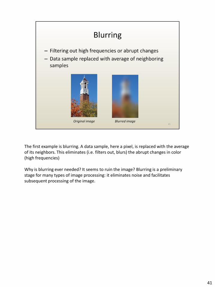
The first example is blurring. A data sample, here a pixel, is replaced with the average of its neighbors. This eliminates (i.e. filters out, blurs) the abrupt changes in color (high frequencies) Why is blurring ever needed? It seems to ruin the image? Blurring is a preliminary stage for many types of image processing: it eliminates noise and facilitates subsequent processing of the image.

41

Sorting is obviously a very important operation that reshuffles data to achieve a certain ordering.

42

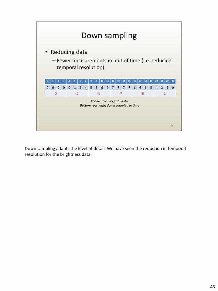
Down sampling adapts the level of detail. We have seen the reduction in temporal resolution for the brightness data.

43

Down sampling can also reduce brightness resolution. Here there are three levels after down sampling. One could also down samples to a single bit per hour, namely is it dark or is it light (0 or 1).

44

Here is another example of down sampling. The down sampled image is 4 times smaller in each direction. There are 4 times fewer pixels in each direction. Since the down sampled image is displayed with pixels of the same size as the original image, the image appears smaller. However, the smaller image shows the same thing as the original image. It still captures the same solid angle of the Purdue Clock Tower scene.

45

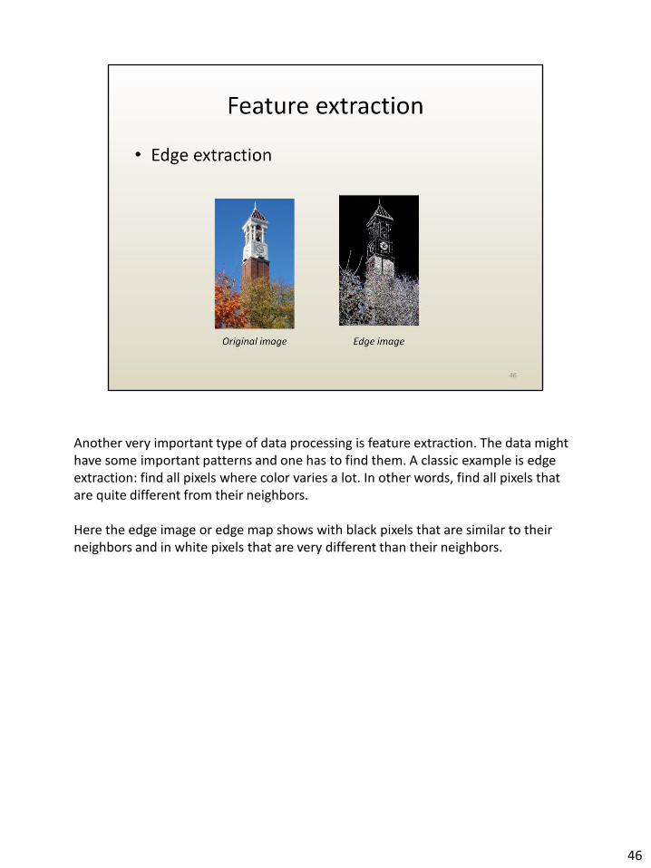
Another very important type of data processing is feature extraction. The data might have some important patterns and one has to find them. A classic example is edge extraction: find all pixels where color varies a lot. In other words, find all pixels that are quite different from their neighbors. Here the edge image or edge map shows with black pixels that are similar to their neighbors and in white pixels that are very different than their neighbors.

46

Another application is to “scramble” data such that no one other than the intended recipient can find it. This means that one has to be able to encrypt, or translate the original data to an intermediate, cryptic, form, and then also to decrypt, or to translate the encrypted data back to the original data. Here is a simple encryption/decryption scheme. Replace a character with the following character to encrypt, and with the preceding character to decrypt. Is it a good encryption / decryption scheme? Not great, foes might guess it.

47

The desirable qualities of an encryption / decryption scheme are: - Hard to break - Lean - Quick

48

Some of you might know that encrypting decrypting data was an important aspect of WWII. The Enigma was a machine used by the German military to encode messages. Code breaking efforts (in Poland, Britain, etc.) aided by hardware and codebook capture are credited for shortening the war in Europe by 2 years.

49

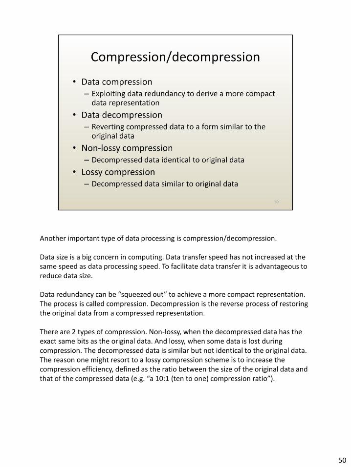
Another important type of data processing is compression/decompression. Data size is a big concern in computing. Data transfer speed has not increased at the same speed as data processing speed. To facilitate data transfer it is advantageous to reduce data size. Data redundancy can be “squeezed out” to achieve a more compact representation. The process is called compression. Decompression is the reverse process of restoring the original data from a compressed representation. There are 2 types of compression. Non-lossy, when the decompressed data has the exact same bits as the original data. And lossy, when some data is lost during compression. The decompressed data is similar but not identical to the original data. The reason one might resort to a lossy compression scheme is to increase the compression efficiency, defined as the ratio between the size of the original data and that of the compressed data (e.g. “a 10:1 (ten to one) compression ratio”).

50

Here is a simple compression / decompression scheme Consider the input data given as a sequence of bits. The compression scheme replaces the original data by an encoding of sub-sequences of identical bits (i.e. either 1 or 0). 10 zeros followed by 4 ones followed by 2 zeros etc This scheme is non lossy. One can recover the exact original data by decompression.

51

A modified scheme will be more efficient, i.e. the compressed data will be more compact, but at the cost of small differences between the original and the decompressed data. Notice here that the sequence of two zeros was discarded and replaced by a sequence of two ones.

52

53

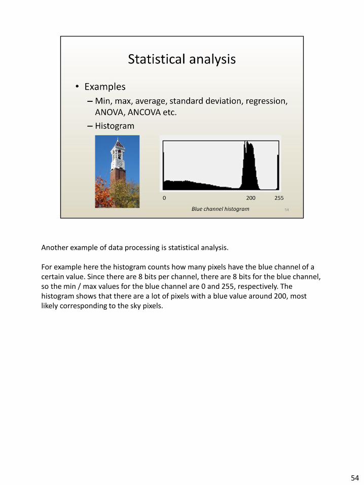
Another example of data processing is statistical analysis. For example here the histogram counts how many pixels have the blue channel of a certain value. Since there are 8 bits per channel, there are 8 bits for the blue channel, so the min / max values for the blue channel are 0 and 255, respectively. The histogram shows that there are a lot of pixels with a blue value around 200, most likely corresponding to the sky pixels.

54