Disability testing and retirement1

Helmuth Cremer, Jean-Marie Lozachmeur and Pierre Pestieau

March 2004, revised November 2004

1An earlier version of this paper has been circulated under the title “Disability, preferencesfor leisure and retirement decision”.

Abstract

This paper studies the design of retirement and disability policies. It illustrates theoften observed exit from the labor force of healthy workers through disability insuranceschemes. Two types of individuals, disabled and leisure-prone ones, have the samedisutility for labor and cannot be distinguished. However, they are not counted in thesame way in social welfare. Benefits depend on retirement age and on the (reported)health status. We determine first- and second-best optimal benefit levels and retirementages and focus on the distortions which may be induced in the individuals’ retirementdecision. Then we introduce the possibility of testing which sorts out disabled workersfrom healthy but retirement-prone workers. We show that such testing can increaseboth social welfare and the rate of participation of elderly workers; in addition disabledworkers are better taken care of. It is not optimal to test all applicants, nor to applytesting to all types of benefits. Surprisingly, the (second-best) solution may imply laterretirement for the disabled than for the leisure prone. In that case, the disabled arecompensated by higher benefits.

1 Introduction

Over the last decade the future of pension systems has been a widely debated issue. The

challenges posed by the ongoing process of demographic aging are by now understood.

However, aging is only part of the story. The generalized decrease of entry ages into

retirement is also a significant problem. There are a number of explanations for this

trend. The dominant one is the implicit taxation on continued activity of elderly workers.

This argument is based on the idea that workers have, individually or collectively, a

large degree of discretion concerning retirement age. In that line, Gruber and Wise

(1999, 2004) have shown for a dozen of OECD countries that households often face very

powerful financial incentives pushing them to retire early.

Some of these incentives may result from the deliberate choice of decision makers:

early retirement schemes in some declining industries, disability insurance for disabled

workers, unemployment insurance for workers who have no chance to find another job.

It might be the case that policy makers have used too much of these policies with the

complicity of unions and management. On some occasions programs might also have

been diverted from their original purpose. For instance, unemployment and disability

insurance have at times been used not only to compensate for “genuine” unemployment

or disability but also to allow healthy and still productive workers to withdraw from

the labor force. When looking at the data on disability — for unemployment, the issue

is trickier — it is clear that they do not only encompass disabled workers. They also

include people who want to stop working and to benefit from a system with slacking

control.

“Flaws” in control can be deliberate or not. They can certainly be due to bad

policy design. However, it is not clear either that a systematic use of tight controls

to all applicants for (say) disability benefits is necessarily the appropriate policy. The

question is where to draw the line between disability benefits, which would be subject

to more or less tight screening, and (early) retirement benefits which are conditional

only on age (and on the individual’s retirement decision). This is one of the questions

discussed in this paper. In particular, we show that without control a number of workers

1

who highly value leisure will use disability insurance as a way to leave the labor market.

This has two consequences: a relatively low age of retirement but more importantly a

relatively low level of disability benefits.

We use a simple model with three different types of individuals with identical produc-

tivity: hard working individuals, retirement-prone individuals and disabled individuals.

At first sight, the latter two look very much alike. However, the disabled have a high

disutility of labor because effort hurts them while the retirement-prone individuals have

the same high disutility because they like leisure. The social planner would like to give

more weight to the disabled than to the two other ones that we will call the hard-working

and the lazy ones. However if it cannot sort out the lazy and the disabled, they will be

given the same package (or at least the same utility level).

We then introduce an audit procedure which allows for such sorting out. More

precisely, there is a testing procedure which reveals individuals health status so that the

disabled can be identified. We show that such control can increase both social welfare

and the rate of participation of elderly workers; in addition disabled workers are better

taken care of. However, we also show that it is not optimal to test all applicants, nor to

apply testing to all types of benefits. To some extent the solution without audit looks

very much like what is observed in a number of countries where there is a clear abuse of

disability insurance programs with the consequence of low participation rate of elderly

workers and with an erosion of disability benefits for budgetary reasons. The solution

with audit looks like what was prevailing at the start of social security programs and

what a number of economists are now advocating to increase the age of retirement: stop

to use disability insurance as an early retirement program.

We have already mentioned the papers which show that disability insurance and

other programs are standard routes for exiting the labor force before the normal retire-

ment age. In addition, there are papers that specifically deal with disability insurance.

In the United States there is a lot of work on the interaction between disability insur-

ance and the labor market. Parsons (1980) in a widely quoted paper shows that social

security program explains a large fraction of the postwar decline in prime-age labor force

participation. This study was followed by several ones which never disputed the disin-

2

centive effects of disability insurance but questioned their magnitude [see e.g. Bound

(1989), Parsons (1980, 1991) and Gruber (2000)]. This literature shows that there are

two issues: one concerns the number of truly disabled workers and the other concerns

the number of beneficiaries from disability insurance. Putting aside employment policy

considerations, the difference between these two numbers comes from the difficulty to

sort out true disabled workers in a world of asymmetric information.

2 A simple model of disability insurance

2.1 Preferences and types of individuals

The setting is inspired by Cremer et al. (2004). Consider an individual with productivity

w, dividing his lifetime with duration normalized to one into a period of full activity

and a period of retirement. Assume away any liquidity constraint and posit zero rate of

interest and time discount rate. The budget constraint is then given by:

1Z0

c (t) dt =

zZ0

w dt,

where c (t) is instantaneous consumption and z (z ≤ 1) the age of retirement. Lifetimeutility is defined as

U =

1Z0

u (c (t)) dt−zZ0

r (t) dt,

where u (·) is a strictly concave instantaneous utility functions while r (t) denotes anincreasing function of effort disutility. As it will appear below r (t) can be viewed as

a mixture of taste for retirement leisure and of physical and mental inability to work

further years. We assume that r (t) varies across individuals and increases over lifetime.

Under these assumptions, the utility function and the budget constraint can be rewritten

as:

U = u (c)−R (z) ,

and

hc = wz,

3

where

R(z) =

Z z

0r(t)dt. (1)

In other words, there is perfect smoothing of consumption over time. We shall use this

reduced form for utility and budget constraint throughout the paper.

There are three types of individuals indexed i = H,L,D. We assume

rH (t) < rL (t) = rD(t) for every t (2)

which from (1) also implies RH(z) < RL(z) = RD(z). Individuals of type H are hard-

working or healthy; they have a low disutility of labor. Type D and L have the same

(high) disutility of labor which is higher than that for type H. They thus have the same

preferences over consumption and leisure. However, they differ in their “health status”.

Specifically, we think of type D as truly disabled for which the high disutility of labor

is due to a poor health. Individuals of type L, on the other hand, are in good health

but are leisure prone (or for short “lazy”). Formally, one can thus think of the health

status as a second dimension of heterogeneity. This heterogeneity is not reflected in the

individuals preferences over consumption and length of activity. However, it determines

the preferences of the social planner who roughly speaking will want to help the disabled

but not the leisure prone individuals; see below for further discussion.

Observe that (2) can also be written as

R0H(z)u0(c)

<R0L(z)u0(c)

=R0D(z)u0(c)

, z ∈ [0, h], c > 0, (3)

which can be interpreted as a single-crossing property. For any bundle in the (z, c) space,

L and D type individuals have steeper indifference curves than H type individuals.

2.2 Policy

We now introduce the possibility of a disability/retirement insurance scheme consisting

of a payroll tax τ and a (pension) benefit function p (z) which depends on the retirement

age. This tax-transfer scheme (τ , p (z)) encompasses disability and retirement insurance

programs. For simplicity we shall often refer to this as “social insurance”. It can be

4

represented by a non linear tax function

T (z) ≡zZ0

wτ dt−1Zz

p (z) dt

= zτw − (1− z) p (z) .

Differentiating T (z) with respect to z yields the marginal tax on postponed work that

underlies the retirement insurance program

T 0 (z) = τw + p (z)− (1− z) p0 (z) .

This expression shows the cost of delaying retirement which is given by τw, the payroll

tax plus p (z), the foregone pension minus the increase in benefit (p0 (z)), if any, over

the length of retirement (1− z). We refer to a social insurance program as “actuarially

neutral” at the margin if T 0 (z) = 0.1

For future reference, note that a consumer’s problem under a non-linear function

T (z) can be written as

maxz

u (wz − T (z))−R (z) . (4)

From the first-order condition we then obtain

R0 (z)u0 (c)

= w − T 0 (z) . (5)

In words, a non-zero marginal tax implies a wedge between the marginal rate of sub-

stitution between work and consumption and the marginal productivity of labor. This

relationship is important for the interpretation of our results below.

3 Indistinguishable types with different social weights

Let us now return to the interpretation of R (z) , that is the disutility for prolonged

activity. This disutility is affected both by taste and by health factors. Some people

want to retire early because they have a strong preference for leisure and desire enjoy

1We use the term “actuarial neutrality” (or fairness) regarding retirement. This has to be distin-guished from fairness (marginal or average) regarding the return from saving, namely the relationbetween contribution and benefit. See on this Crawford and Lilien (1981) and Desmet and Jousten(2003).

5

a long retirement period. Some other people want to retire because physically they

cannot work longer. To account for this apparent ambiguity, we distinguish disabled

(D) and leisure-prone individuals (L). Clearly if disability were easily observable there

would be no problem. There are however cases when it is only observable at some cost,

the cost of medical tests.

Recall that D and L have the same function Ri (z); in other words RL (z) = RD (z).

However the social planner is not ready to consider those two types as identical. We

assume that the social planner wants to help the disabled workers but not the leisure-

prone ones. More precisely, the high disutility for prolonged activity is considered as

“legitimate” (and fully accounted for in welfare) for the disabled but not for the lazy

individuals.2 One way of introducing such a distinction is to assume a weighted social

welfare function with lower weights on type L than on type D. This leaves open the issue

of which weight to attach to H. To keep things simple, we introduce welfare weights

ϕi (i = H,L,D) such that ϕL < ϕD = ϕH . A possible justification of this choice is

to think that there is a majority of people who ex ante do not know whether they

are H or D. They maximize their expected utility with some limited concern for a

minority of leisure-prone workers who will never be disabled. An alternative approach

with paternalistic rather than Paretian social preferences is considered in Section 4

where the disutility for the lazy type L is evaluated with RH rather than RL.

3.1 Full information optimum and laissez-faire

Denoting pi the proportion of type i individuals, the first-best problem is given by:

maxci,zi

Xi

ϕipi [u (ci)−Ri (zi)] + µXi

pi (wzi − ci) . (6)

This gives the efficiency conditions:

R0H (zH)u0 (cH)

=R0L (zL)u0 (cL)

=R0L (zD)u0 (cD)

= w, (7)

2The assumption that RL (z) = RD (z) is not important for our analysis. It is made for simplicitybecause it yields crisper results in some cases. The crucial feature of our model is that the two typesare treated differently in the social welfare function. See also footnote 4

6

which, not surprisingly, are equivalent to (5) with T 0(z) = 0. With objective (6) the

social optimum is Pareto efficient and we have the usual first-best tradeoffs.

We also have:

ϕH u0 (cH) = ϕL u0 (cL) = ϕD u0 (cD) = µ, (8)

so that consumption levels and retirement ages are ranked as follows:

cD = cH > cL

zD < zH zD < zL zH ≷ zL.

With this specification type D ’s individuals end up retiring earlier than the two other

ones. They consume as much as H and more than L. In other words they are compen-

sated for their disability not only by retiring earlier but also by receiving higher benefits

(which is conceivable in a social insurance setting).

The laissez-faire solution does not depend on the social objective. Consequently it

is given by equations (7) with the implication that cD = cL < cH and zD = zL < zH .

Observe that to decentralize the full information solution, one simply needs lump-sum

transfers from H and L to D and between H and L (the direction depending on the

weights). The retirement choice does not have to be distorted. This is because the

weighted objective function necessarily yields a Pareto-efficient solution so that the

second welfare theorem applies.

3.2 Unobservable types: second-best solution

Let us now turn to the second-best problem, where types are not observable. With

three types, we then have to add six incentive compatibility constraints.3 In particular,

we have

u (cL)−RL (zL) ≥ u (cD)−RL (zD) (9)

for type L and

u (cD)−RD (zD) ≥ u (cL)−RD (zL) (10)

3Each type can potentially mimick either of the two other types.

7

for type D. Recalling that RL (z) ≡ RD(z) and combining (10) and (9) yields not

surprisingly:

u (cL)−RL (zL) = u (cD)−RL (zD) . (11)

In words, because D and L have the same preferences over c and z, their utility levels

must be equalized at any incentive-compatible allocation. The simplest way to achieve

(11) is of course to offer the same consumption bundle to the two types cL = cD and

consequently zL = zD. As will become clear below, this is effectively optimal even when

it is not a priori imposed.4

When types D and L are pooled, the problem of the social planner is

maxXi

ϕipi [u (ci)−Ri (zi)] + µXi

pi (wzi − ci)

+ λ [u (cH)−RH (zH)− u (cL) +RH (zL)]

where we use the subscript L for both L and D’s choices of z and c. The FOC with

respect to zH and cH yield the traditional no distortion at the top: the marginal rate of

substitution of type H continues to be given by (7). The FOC with respect to zL = zD

and cL = cD yield:

R0L (zL)u0 (cL)

= w − λ

(ϕLpL + ϕDpD − λ)

[R0L (zL)−R0H (zL)]u0(cL)

. (12)

where (ϕLpL + ϕDpD − λ) > 0 follows from the FOC with respect to cL = cD, while

the single-crossing property (3) implies R0L (zL) > R0H(zL). Consequently, we have a

downward distortion and a positive marginal tax on zL = zD. We have a rather standard

optimal tax problem. A distortion on z is here only justified by incentive arguments.

Per our assumptions on preferences, a downward distortion is called for to relax an

otherwise binding self-selection constraint.

3.3 Second-best with auditing

It is pretty clear that the lack of observability of the health status can be quite costly

in terms of welfare. It is particularly detrimental to the disabled workers. Because they4That is when any bundles (cL, zL) and (cD, zD) satisfying (11) are permitted. We do not prove

this property here because the easiest proof makes use of the FOC derived in the next subsection; seeRemark 1 in Appendix A1. Observe that such a pooling may also arise when D and L do not haveidentical preferences.

8

are pooled with the leisure-prone ones they are forced to work longer and receive less

benefits than they would otherwise in a world of perfect observability.

To improve upon this second-best solution, one has to find ways to distinguish types

L and D. A traditional way to achieve this is to use disability evaluations.5

To study the implication of such a policy, we adopt a very simple form of audit which

perfectly reveals an individual’s “health status”.6 More precisely, the audit indicates

whether or not an individual is of type D. In particular, it can be used to distinguish

between D and L individuals. Observe that the audit also reveals mimicking between

H and D, but not between H and L (who are both in good health). When a fraction

π of type D’s reports are subject to testing, the corresponding audit cost is given by

k(pDπ). An individual who is caught cheating is subject to a sanction which reduces

his utility to some exogenous and “low” utility level of u¯. With this assumption, we

have to modify the revenue constraints of the government and consider six incentive

compatibility relations: Xi

pi (wzi − ci)− k(pDπ) = 0

(LD) : u (cL)−RL (zL)− (1− π) (u (cD)−RL (zD))− πu¯> 0

(DL) : u (cD)−RL (zD)− u (cL) +RL (zL) > 0

(HD) : u (cH)−RH (zH)− (1− π) (u (cD)−RH (zD))− πu¯> 0

(DH) : u (cD)−RL (zD)− u (cH) +RL (zH)

(HL) : u (cH)−RH (zH)− u (cL) +RH (zL) > 0

(LH) : u (cL)−RL (zL)− u (cH) +RL (zH) > 0.

The properties of the solution will of course depend on which of the incentive con-

straints are binding at the optimum. With six incentive the number of potential com-5An alternative way, considered by Marchand et al. (2003), is to observe the consumption vectors of

both types which surely reveal their differences. One can on that basis self-select the two types with asolution that can be implemented with non-linear taxes on consumption and income.

6There is some literature on this. In general the tests are imperfect generating errors of types 1 and2; see Diamond and Sheshinski (1995) and Parsons (1996). As long as the probability of audit is lowerthan one, our audit process implies three categories of individuals: able (or leisure-prone) individualswho are not audited and disabled individuals who are either audited or not. In Diamond and Sheshinski(1995) the two latter groups may contain able individuals because of type 1 and 2 errors in the auditprocess. This difficulty does not arise in our setting where audits are perfect.

9

binations of binding incentive constraint is quite large. To reduce the number of cases

we shall first of all make some rather plausible assumptions. First, we assume that the

weights are such that the “upwards” constraints (DH) and (LH) are not binding. With

ϕD = ϕH > ϕL it is clear that (LH) can potentially be binding when the weight on

L becomes very small. We assume that this is not the case. Second, we shall restrict

our attention to settings where (LD) is binding. This, in turn immediately implies that

(DL) is not binding (as long as π > 0).

The Lagrangian expression associated with the problem of the social planner is then

given by:

L1 =Xi

ϕipi [u (ci)−Ri (zi)] + µ

"Xi

pi (wzi − ci)− k(pDπ)

#+ λLD [u (cL)−RL (zL)− (1− π) (u (cD)−RL (zD))− π u

¯]

+ λHL [u (cH)−RH (zH)− u (cL) +RH (zL)]

+ λHD [u (cH)−RH (zH)− (1− π) (u (cD)−RH (zD))− π u¯]

The FOC are provided in Appendix A1; they can be rearranged as follows:

MRSH =R0H (zH)u0 (cH)

= w (13)

MRSL =R0L (zL)u0 (cL)

= w − λHL [R0L (zL)−R0H (zL)]

(ϕLpL + λLD − λHL)u0(cL)≤ w (14)

MRSD =R0D (zD)u0 (cD)

= w − λHD (1− π) [R0L (zD)−R0H (zD)]ϕDpD − (λLD + λHD) (1− π)u0 (cD)

≤ w (15)

In the Appendix, we use these first-order-conditions to derive the following lemma which

further reduces the number of regimes to be considered.

Lemma 1 A solution with λHD > 0 and λHL = 0 is not possible.

Lemma 1 along with the assumption made above imply that we are left with the

following three regimes.

Regime Binding incentive constraints1 (HL),(HD),(LD)2 (HL),(LD)3 (LD)

10

The numerical illustrations provided in the next subsection show that each of these

three regimes can effectively occur. From the fist-order-conditions we then obtain the

following results for the different types of individuals.

Type H Whatever the regime we have from (13) that the marginal tax on z is zero

for the type H individual. This is the usual no distortion at the top result which arises

because no incentive constraint towards these individuals is binding.

Type L We obtain from (14) that this individual is subject to a downward distortion

on their choice of retirement if (and only if) λHL > 0 that is in Regimes 1 and 2.

Type D Using (15) we see that there may or may not be a distortion in the choice

of z for this type, depending on λHD. When λHD > 0, zD is subject to a downward

distortion which does not come as a surprise. This occurs in Regime 1 only. In the

two other regimes where λHD = 0 individuals of type D are subject to no distortion.

This may appear surprising at first because an incentive constraint towards D, namely

(LD) is binding. However, since D and L have the same indifference curves, a distortion

would not be an effective way to relax this incentive constraint.7

An interesting question which arises is whether the introduction of audit makes the

lazy retire later than the disabled? The answer depends on the regime. In Regime 3,

neither type D or L are subject to distortions. Since type D workers are on a higher

indifference curve, we unambiguously have zL > zD. In Regime 2, there in an implicit

tax on zL but the disabled receive a higher transfer than the lazy. These transfers have

an effect that fosters early retirement so that the comparison between zL and zD is

ambiguous. In Regime 1 where the comparison between zD and zL seems ambiguous

(both being distorted downwards), we can rank them unambiguously. To see this, we

write (HL) , (LD) and (HD) as equalities and combine them, yielding:

RL (zL)−RH (zL) = (1− π) [RL (zD)−RH (zD)] . (16)

7To be more precise, the mimicked individual would be hurt as much as the mimicker. Consequently,a distortion cannot be welfare-improving.

11

The LHS of this expression is the utility differential between H and L at L ’s consump-

tion bundle. It gives the rent which must be conceded to H to prevent mimicking of L.

The RHS is also a utility differential between H and L but at D’s consumption bundle.

This shows the extra rent H must be granted compared to L at a solution where both

types are prevented from mimicking D. This second rent is weighted by the probability

of not being detected by the audit since types H and L are subject to audit when mim-

icking type D. Not surprisingly, when (HL) , (LD) and (HD) are binding the two rents

in (16) are equalized. These two rents being increasing in z by convexity of R (.), one

has zD > zL. Consequently, in Regime 1 we do have the result that disabled individuals

retire later than the lazy ones.

All these results are valid for any arbitrary level of the audit probability (0 < π < 1).8

To determine the optimal level of π, we have to use the first-order condition (A7). It

shows that the determination of π involves a tradeoff between costs (µpDk0) and benefits

that depend on the utility gap between truthtelling and being caught. Quite evidently

the larger the audit costs, and the larger u¯the lower will be π. Conversely, the lower

the audit costs, the higher will be π. Note, however, that auditing with probability

one (π = 1) is never optimal. This is a standard result in auditing models. It directly

follows from (A7) by observing that when π = 1, (LD) and (HD) are satisfied with

strict inequality consequently we would have λLD = λHD = 0 which implies that the

derivative is negative. This makes sense, when incentive constraints are satisfied with

strict inequality, they continue to be satisfied when audit probability (and hence audit

cost) is slightly reduced.

Not much can be said analytically about the factors explaining the occurrence of

one regime rather than another. However, it is clear that π, which in turn is determined

by audit costs will play a crucial role. In particular, when π is high enough, Regime 1

cannot occur. To see this suppose that (LD) and (HL) bind. Using the expressions for

the incentive constraints it follows that (HD) is not binding when

RL (zL)−RH (zL)− (1− π) [RL (zD)−RH (zD)] > 0. (17)

8Consequently, they also apply when the audit probability is exogenously given (rather then set atits optimal level).

12

c

0 wz

d = l l

45°

c

0 wz

h

d = l l

d

45°

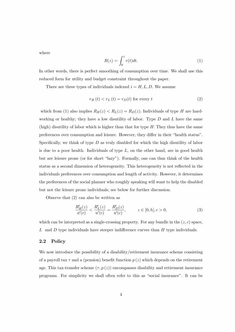
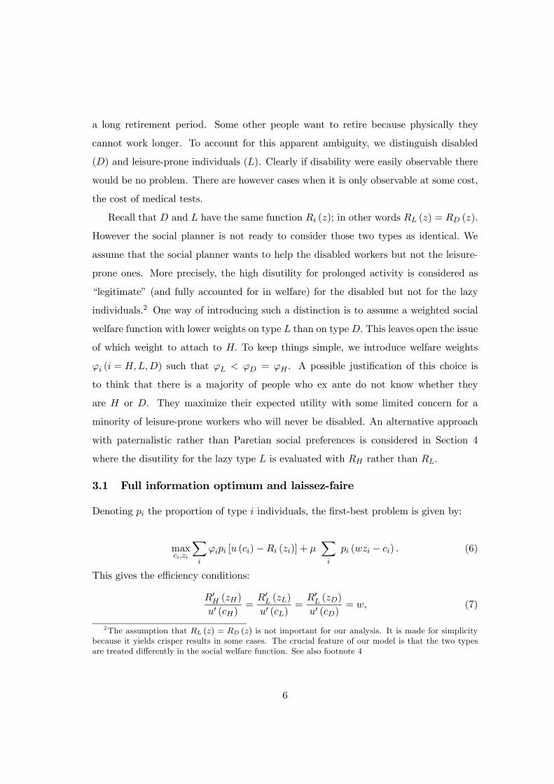
Figure 1: Solution without and with auditing.

which necessarily holds when π is close to one.

Figure 1 illustrates the above solution for Regime 2 as well as the solution without

audit studied in Subsection 3.2. Without audit, individuals of type H consume the

bundle h and the individuals D and L who cannot be distinguished consume = d.

With audit, we have and d for the lazy and the disabled respectively. Now the disabled

could get a consumption level as high as that of the individuals h. However, while this

would be true at the first-best, it is of course not desirable in a second-best setting.9

With λHD = 0 (Regime 2), individuals D do not face any distortion.10 The comparison

between zD and zL is ambiguous. Type D individuals are on a higher indifference

curve; this income effect decreases labor supply. Type L individuals are subject to

a positive marginal tax which tends to decrease labor supply. Summing up, one can

expect individuals of type D to work less (retire earlier) then individuals of type L if the

income effect is sufficiently important (or if audit probability is large). The individuals

L work more and consume also more than in the pooling equilibrium. We now turn to

a numerical illustration.9This follows directly from (A1) and (A3).10Regime 1 yields a similar representation, except that D now faces a distortion.

13

3.4 Illustration

The functional form we use is given by:

u (ci, zi) = ln ci − αiz2i2,

with the following parameter values

H L D

αi 1 5 5pi 0.6 0.1 0.3ϕi 1 0.3 1wi 100 100 100

We consider three audit technologies depending on their cost: audit 1 is relatively

expensive¡k (π) = 2000π2

¢and implies π = 0.06, λHL > 0 and λLD > 0 and λHD > 0

(Regime 1); audit 2 is cheaper¡k (π) = 1000π2

¢and implies π = 0.10 with λHL > 0

and λLD > 0 (Regime 2). Finally audit 3 is the cheapest¡k (π) = 100π2

¢and implies

π = 0.49 (and Regime 3). In all cases, u = 0. The results are given in Table 1.

First-best PoolingTypes D L H D L H

c 88.39 26.51 88.39 54 54 92.48z 0.22 0.75 1.13 0.30 0.30 1.08u 4.35 1.85 3.84 3.75 3.75 3.94

T 0 (z) 0 0 0 0.17 0.17 0

Audit 1 Audit 2 Audit 3Types D L H D L H D L H

c 65.29 49.72 89.32 70.74 48.23 87.94 81.42 46.59 84.95z 0.29 0.28 1.11 0.28 0.30 1.13 0.24 0.43 1.17u 3.95 3.70 3.86 4.05 3.64 3.83 4.24 3.38 3.74

T 0 (z) 0.03 0.28 0 0 0.26 0 0 0 0

Table 1: Numerical example, Paretian objective

First, observe that starting from the no auditing pooling solution, introducing audit

1 leads to Regime 1 where all three incentive compatibility constraints are binding.

Turning to a less expensive technology (and thus to a higher level of audit) implies a

14

regime where (HD) no longer binds. This illustrates the argument we made on the basis

of (17). For even smaller audit costs we obtain Regime 3. Observe, however, that if the

audit technology would be completely costless, we would have either only (HL) binding

if ϕL is relatively high or the first best if ϕL is relatively low11.

Second, we observe that in all the second-best solutions the consumption of D is

kept below that of H whereas in the first-best the two types have the same consumption.

Not surprisingly, the difference between cH and cD decreases as the audit probability

increases. Furthermore, in the pooling solution we have cD = cL while with auditing

cD > cL holds; as expected the difference between cD and cL increases as audit become

cheaper and more intense and thus allows for a better screening. Finally, in Regime 1

D retires later than L which is in line with the analytical result obtained above. In the

other two regimes, however, we have zD < zL, even though L faces a positive marginal

tax in Regime 2 while D’s marginal tax is zero. This illustrates the idea that the income

effects (transfer to D) can dominate the substitution effects (marginal distortions).

4 Alternative specification

We now consider an alternative specification wherein the social planner paternalistically

attributes to the lazy workers a disutility RL rather than RH . In other words, he wants

them to work more and not to consume less. Once again, we start by considering the

full information solution.

4.1 Full information solution and decentralization

With the paternalistic approach the full information problem is given by:

maxXi

piu (ci)− pHRH (zH)− pLRH (zL)− pDRL (zD) + µXi

pi (ci −wzi) .

The solution is easily obtained. Both healthy types (namely H and L) are assigned the

same retirement age, the disabled individuals retire earlier and all individuals have the

11 If the first best allocation described in section 3.1 respects (HL) then the first best allocation isimplementable with audits. If it is not (which is the case if ϕL is high enough) then (HL) would bindwith free audit.

15

same consumption level:

zD < zL = zH and cD = cL = cD.

The laissez-faire solution does not depend on the social objective and is thus the

same as in Subsection 3.1. Consequently it is given by equations (7) with the implication

that cD = cL < cH and zD = zL < zH . Decentralizing the first-best, however, is now

not as simple as in the non-paternalistic specification. Lump sum transfers are not

sufficient; one also needs a subsidy (negative marginal tax), on the labor supply of type

L individuals. To see this, note that the decentralized choice of zL is determined by:

(w − T 0 (zL))u0 (cL)−R0L (zL) = 0 (18)

which coincides with the socially optimal one

w u0 (cL)−R0H (zL) = 0. (19)

when the marginal tax rate is given by

T 0 (zL) = − [R0L (zL)−R0H (zL)]

u0(cL)< 0, (20)

so that we effectively have a subsidy. In words, the rate of subsidy is equal to the

difference between “private” and the “social” marginal valuation for zL (evaluated at

the optimal allocation). Paternalism introduces a wedge between private and social

valuation of type L’s labor supply and the decentralization of the optimum requires a

“Pigouvian” subsidy.

4.2 Unobservable types: second-best solution

Let us now turn to the second-best problem, where types are not observable. With

three types, we then have to consider six incentive constraints. As in Section 3, we start

with the no-audit case, for which one can show that only (HL) , (HD) and (LD) can

possibly be binding.12 Clearly, when (HD) is binding together with (HL) and (LD) ,

12 In other words the upwards constraint (LH) and (DH) cannot be binding. While this property isnot surprising, its proof is somewhat tedious. It is omitted here but is available from the authors uponrequest.

16

one has a pooling optimum. The program is now:

maxX

pi u (ci)− pH RH (zH)− pL RH (zL)− pD RL (zL)

+ µX

pi (wzi − ci) + λHL [u (cH)−RH (zH)− u (cL) +RH (zL)]

+ λHD [u (cH)−RH (zH)− u (cD) +RH (zD)]

+ λLD [u (cL)−RL (zL)− u (cD) +RL (zD)]

The first-order conditions with respect to zH and cH yield the traditional no distortion

at the top result: the marginal rate of substitution of type H continues to be given by

(7). The FOC with respect to zL, zD, cL and cD are:

(pL − λHL + λLD)u0 (cL) + µpL = 0 (21)

(pD − λHD − λLD)u0 (cD) + µpD = 0 (22)

− pLR0H (zL)− µpLw + λHLR

0H (zL)− λLDR

0L (zL) = 0 (23)

− pDR0L (zD)− µpDw + λHDR

0H (zD) + λLDR

0L (zD) = 0 (24)

This yields:

MRSL =R0L (zL)u0 (cL)

= w +

·pL − λHL

pL − λHL + λLD

¸ ·R0L (zL)−R0H (zL)

u0 (cL)

¸, (25)

where pL−λHL+λLD > 0 from (21) while the sign of (pL−λ) appears to be ambiguous.Furthermore we have

MRSD =R0D (zD)u0 (cD)

= w − λHD

(pD − λLD − λHD)

·R0L (zD)−R0H (zD)

u0 (cD)

¸(26)

where (pD−λLD−λHD) > 0 from (22) so that we necessarily have a downward distortion

for type D’s choice of z. The new feature which arises here is that D and L are no longer

necessarily pooled even when there is no audit. More precisely, we have

Lemma 2 The optimum pools D and L if and only if R0L (zL) /u0 (cL) < w that is iff

pL < λHL.

To interpret this result, consider equation (25). The distortion on zL is of ambiguous

sign. When pL > λHL, the RHS of (25) is larger than w so that we have an upward

17

distortion on labor supply (a negative marginal tax rate). Conversely, pL < λHL yields a

downward distortion and thus a positive marginal tax. To understand the role played by

this term, note that the distortion in type L’s labor supply is determined by balancing

two conflicting objectives. First, there is the standard (Mirrlees-type) incentive effect

which calls for a downward distortion (positive marginal tax) on L’s labor supply in

order to relax the incentive constraint from type H to type L. The significance of this

effect depends on λHL, the Lagrange multiplier of this incentive constraint. Second,

there is a “paternalistic” effect, which calls for an increase in type L’s labor supply

compared to the laissez-faire level. Recall, that social disutility of their labor is smaller

than their private disutility. This pleads in favor of an upward distortion (a negative

marginal tax). This effect is the more significant, the larger the proportion of group L

in the economy. When pL is large enough, the paternalistic consideration is dominant

so that there is a marginal subsidy on zL. In this case, there is no reason to pool

individuals L and D because there is no need of distortion on zD. However, when pL is

small, incentive considerations dominate and a marginal tax is called for on zL. In this

case, one necessarily pools individuals L and D in order to prevent individuals H from

mimicking individuals D.

To sum up, when pL is large enough, the optimum entails separation between type

D and L individuals. In this case, there is no distortion on zD and a marginal subsidy

on zL. When pL is small, one has a pooling optimum with a marginal tax on zL and

zD. Note finally, that in the separating optimum, one necessarily always has zL > zD.

4.3 Second-best with audit in the paternalistic case

Introducing audit as in Section 3, while continuing to assume that the upwards con-

straints (LH) and (DH) are not binding, the social planner problem can now be written

18

as the maximization of:

L2 =3X

i=1

piu (ci)− pHRH (zH)− pLRH(zL)− pDRL(zD)

+µ

"3X

i=1

pi(wzi − ci)− pDkπ

#+λLD[u (cL)−RL (zL)− (1− π) (u (cD)−RL (zD))− πu]

+λHL [u (cH)−RH (zH)− u (cL) +RH (zL)]

+λHD [u (cH)−RH (zH)− (1− π) (u (cD)−RH (zD))− πu]

+λDL [u (cD)−RD (zD)− u (cL) +RD (zL)]

The FOC are stated Appendix A3. Combining and rearranging these conditions yield

the following expressions for the marginal rates of substitution of the different types:

R0H (zH)u0 (cH)

= w. (27)

R0L (zL)u0 (cL)

= w +(pL − λHL) [R

0L (zL)−R0H (zL)]

(pL + λLD − λDL − λHL)u0(cL)S w (28)

R0L (zD)u0 (cD)

= w − λHD (1− π) [R0L (zD)−R0H (zD)](pD − (λLD + λHD) (1− π) + λDL)u0 (cD)

≤ w. (29)

Before commenting on these expressions, it is necessary to determine the possible

regimes. To reduce the number of cases, we can first note that Lemma 1 continues

to hold in the alternative specification.13 Next, Appendix A5 provides a sequence of ad-

ditional Lemmas which show that in the paternalistic case, only two regimes are possible

which are given by:

Regime Binding incentive constraints1 (HL), (HD), (LD)

2 (HL), (LD)

Consequently, it turns out that Regime 3, where only (LD) was binding cannot arise

here.

Let us now turn to the interpretation of conditions (27)—(29) while taking into ac-

count that in both possible regimes (DL) is not binding so that we have λDL = 0.

13The proof in Appendix A2 does not rely on the objective function of the government.

19

Equation (27) is the usual no distortion at the top property. Turning to (28) observe

that (pL + λLD − λHL) > 0 from (A12), while (pL − λHL) is ambiguous. As in the

preceding section, when pL > λHL, paternalistic considerations are dominant and call

for a marginal subsidy on zL. When pL < λHL, incentive considerations dominate and

a positive marginal tax on zL is optimal.

For the interpretation of (29), on the other hand, we have to distinguish Regime 2

with λHD = 0 from Regime 1 with λHD > 0. The results are exactly like in Section 3.

In Regime 2, λHD = 0, there is no distortion in the choice of retirement for the truly

disabled. The mimicking individual L has the same indifference curves as individual

D. Consequently, there is no way to create a distortion which hurts the mimicker more

than the mimicked. Put differently a distortion is not an effective way to relax the

incentive constraint. Consequently, the retirement choice of type D is treated at the

margin exactly like that of the type H individual (zero marginal tax). In Regime 1, on

the other hand, we have λHD > 0, and there is a distortion towards earlier retirement.

This distortion relaxes the incentive constraint (HD). As in Section 3, this distortion

is likely to be effective for a relatively low probability of auditing.

The comparison between zL and zD is the same as in Section 3. Note however that

Regime 1 cannot occur when there is a marginal subsidy on zL. To see this, recall that

Regime 1 implies a distortion on zD and zL < zD. Since D is on a higher indifference

curve, this is incompatible with a marginal subsidy on zL. We summarize this in the

following lemma:

Lemma 3 When pL > λHL, Regime 1 cannot occur.

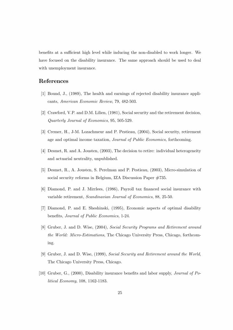
Figure 2 provides a graphical representation of the problem with auditing. On the

figure we have three points in the (y, c) space. The consumption bundle for individuals

of typeH is represented by h, where the slope of the indifference curve is 1. The distance

between h and the (no tax) budget line c = wz is the transfer individuals of type H

have to pay. Point is the solution for individuals of type L with slope different from 1.

We have represented the case where the slope is higher than 1, but it could have been

less. Here individuals L are subject to a marginal subsidy and receive a transfer. Note

20

wz

c

45°

d h

l

Figure 2: Paternalistic objective: solution with auditing

the binding incentive constraint form H to L and the relative slope at of these two

types indifference curves. Finally, d is the solution for individuals of type D. The slope

is 1 (no distortion as for individuals H); they receive a larger transfer than individuals

L. They also work less (d is to the left of ). Note however that with a positive marginal

tax on L and a weak income effect, it is not impossible to have zD > zL in the second

best (recall that it is always the case in Regime 1). Finally, the indifference curve going

through is a linear combination of that going through d and one yielding a level of

utility u.

Equation (A16) determines the optimal value of π which depends on both k, the

cost of auditing, and u¯, the penalty. Not surprisingly, the optimal audit probability

(for type D reports) is determined by the tradeoff between its negative effect on public

expenditures (−µpDk) and its positive effect via the welfare gain stemming from less

stringent IC constraints.

21

First best No auditTypes D L H D L H

c 86.74 86.74 86.74 57.72 57.72 94.04z 0.28 1.15 1.15 0.39 0.39 1.06u 4.29 1.80 3.79 3.74 3.74 3.97

T 0 (z) 0 −3 0 0.09 0.09 0

Audit 1 Audit 2π = 0.04, Regime 1 π = 0.08, Regime 2

Types D L H D L H

c 65.35 54.05 91.55 68.06 53.70 90.59z 0.38 0.37 1.09 0.36 0.41 1.10u 3.88 3.71 3.92 3.95 3.63 3.89

T 0 (z) 0.003 0.19 0 0 0.11 0

Table 3: Numerical example: Paternalistic objective, Scenario 1.

4.4 Illustration: paternalistic objective

We use the same utility function as in Section 3 and continue to assume u = 0. However

in order to illustrate the pooling and the separating optima, we will consider the two

following scenarios for the parameter values:

Scenario1 Scenario2H L D H L D

αi 1 4 4 1 4 4pi 0.6 0.07 0.33 0.6 0.2 0.2wi 100 100 100 100 100 100

These two scenarios differ in the proportion of type L and D in the economy. In

Scenario 1, there is a small proportion of type L individuals while this proportion is

larger in Scenario 2. In addition, we consider two audit technologies depending on

their cost: Audit 1 is relatively expensive¡k (π) = 2000π2

¢while Audit 2 is cheaper¡

k (π) = 1000π2¢. The results are given in Table 3 (Scenario 1) and Table 4 (Scenario

2).

Not surprisingly, Audit 1 implies lower audit probabilities than Audit 2. In scenario

1, pL is relatively low so that without audit, a pooling optimum will occur with a positive

marginal tax on zL and zD. As in the case of the Paretian objective, as audits increase,

one goes from Regime 1 to 2. In Regime 1, lazy individuals will work less than the

22

FirstBest No auditTypes D L H D L H

c 92.19 92.19 92.19 52.20 70.07 97.8z 0.27 1.08 1.08 0.47 0.61 1.02u 4.37 2.17 3.93 3.49 3.49 4.06

T 0 (z) 0 −3 0 0 −0.71 0

Audit 1 Audit 2π = 0.12, Regime 2 π = 0.20, Regime 2

Types D L H D L H

c 60.54 70 95.67 67.20 71.50 94.42z 0.41 0.68 1.04 0.37 0.75 1.05u 3.76 3.31 4.01 3.93 3.13 3.98

T 0 (z) 0 −0.91 0 0 −1.15 0

Table 4: Numerical example: Paternalistic objective, Scenario 2.

disabled while in Regime 2 they turn to work more.

In scenario 2, the optimum without audit involves separation between individuals

D and L. This is because pL is now relatively high so that paternalistic considerations

dominate. In this case, the second best without and with audit involves no distortion

on zD while a marginal subsidy is called for on zL.

5 Conclusion

We have studied the design of retirement cum disability benefits in a three type setting.

Healthy individuals have a low disutility of labor (continued activity). The two other

types have identical preferences with a high disutility of labor. However, they differ in

their (unobservable) health status. Type L individuals have a high disutility for labor

because they are leisure prone. Type D individuals, on the other hand, have a high

disutility because they are disabled. We start from the premise that policy makers are

not prepared to treat types D and L alike. Helping type D individuals and allowing

them to retire early with “generous” benefits is considered as legitimate. However,

society does not want to extend such a generous treatment to the L type individuals.

Formally, this is introduced by considering either a (Paretian) social welfare function

23

which puts less weight on the type L individuals, or by using a paternalistic social

welfare function which does not fully account for the type L individual’s disutility of

labor.

In either setting, a first-best solution would imply earlier retirement for D than for

L (zD < zL). However, when the health status is not observable, it may or may not be

possible to separate the two types out, so that the second-best may imply zD = zL. In

that case, the effectiveness of disability benefits is severely undermined by the presence

of the L type and the possibilities to help the disabled are limited. The situation can

be improved if costly audits (test for disability) become available. However, the second-

best with audit does not necessarily imply zD < zL; quite surprisingly, we may even

end up with a situation where the disabled retire later than the lazy (zD > zL). But

their consumption or rather their disability benefits are higher than those of workers of

type L. Another interesting finding of our analysis is that the optimum often implies

distorted retirement decision at least for types L and D. However, there are situation

in which there are no distortion, even in the second best, or where the distortions affect

only one of the types. We show that this depends on the pattern of binding incentive

constraints which in turns depends on how costly the audit is.

To put these results in perspective, it is interesting to consider the policy implica-

tions of the NBER and OECD studies explaining early retirement by a too extensive use

of social insurance programs is that one should make the overall system more neutral

towards retirement decisions. Demographic aging makes such a reform extremely press-

ing. The problem with such a linear reform is that it is clearly legitimate as it regards

workers who are not disabled nor involuntarily unemployed. It makes economic sense to

decrease the generosity of social insurance programs for those who “abuse” the system.

However, for those who are truly disabled or unemployed, such a reform necessarily

implies lower benefits and this is questionable. From a public finance viewpoint, the

reform works; from a social welfare viewpoint, it is likely to be catastrophic.

What we show in this paper is that to avoid such an outcome one should introduce

or strengthen the audit and control techniques allowing to sort out leisure-prone workers

and true disabled individuals. So doing one can at the same time keep the disability

24

benefits at a sufficient high level while inducing the non-disabled to work longer. We

have focused on the disability insurance. The same approach should be used to deal

with unemployment insurance.

References

[1] Bound, J., (1989), The health and earnings of rejected disability insurance appli-

cants, American Economic Review, 79, 482-503.

[2] Crawford, V.P. and D.M. Lilien, (1981), Social security and the retirement decision,

Quarterly Journal of Economics, 95, 505-529.

[3] Cremer, H., J-M. Lozachmeur and P. Pestieau, (2004), Social security, retirement

age and optimal income taxation, Journal of Public Economics, forthcoming.

[4] Desmet, R. and A. Jousten, (2003), The decision to retire: individual heterogeneity

and actuarial neutrality, unpublished.

[5] Desmet, R., A. Jousten, S. Perelman and P. Pestieau, (2003), Micro-simulation of

social security reforms in Belgium, IZA Discussion Paper #735.

[6] Diamond, P. and J. Mirrlees, (1986), Payroll tax financed social insurance with

variable retirement, Scandinavian Journal of Economics, 88, 25-50.

[7] Diamond, P. and E. Sheshinski, (1995), Economic aspects of optimal disability

benefits, Journal of Public Economics, 1-24.

[8] Gruber, J. and D. Wise, (2004), Social Security Programs and Retirement around

the World: Micro-Estimations, The Chicago University Press, Chicago, forthcom-

ing.

[9] Gruber, J. and D. Wise, (1999), Social Security and Retirement around the World,

The Chicago University Press, Chicago.

[10] Gruber, G., (2000), Disability insurance benefits and labor supply, Journal of Po-

litical Economy, 108, 1162-1183.

25

[11] Marchand, M., P. Pestieau and M. Racionero, (2003), Optimal redistribution when

different workers are indistinguishable, Canadian Journal of Economics, forthcom-

ing.

[12] Parsons, D., (1980), The decline of male labor force participation, Journal of Po-

litical Economy, 88, 117-134.

[13] Parsons, D., (1991), The health and earnings of rejected disability insurance appli-

cants: comment, American Economic Review, 81, 1419-1426.

[14] Parsons, D.O (1996), Imperfect ’tagging’ in social insurance programs, Journal of

Public Economics, 62, 183-207.

[15] Roemer, J., (1998), Equality of Opportunity, Harvard University Press, Cambridge.

26

Appendix

A1 First-order conditions for L1Differentiating L1 yields the following FOC:

∂L1∂cH

= ϕH pH u0 (cH)− pH µ+ (λHL + λHD)u0 (cH) = 0 (A1)

∂L1∂zH

= −ϕH pH R0H (zH) + pH µ w − (λHL + λHD)R0H (zH) = 0 (A2)

∂L1∂cL

= ϕL pL u0 (cL)− pL µ+ (λLD − λHL )u0 (cL) = 0 (A3)

∂L1∂zL

= −ϕL pL R0L (zL) + pL µ w − λLD R0L (zL) + λHL R0H (zL) = 0 (A4)

∂L1∂cD

= ϕD pD u0 (cD)− pD µ− (λLD + λHD) (1− π) u0 (cD) = 0 (A5)

∂L1∂zD

= −ϕD pD R0L (zD) + pD µ w + λLD (1− π) R0L (zD)

+ λHD (1− π)R0H (zD) = 0 (A6)∂L1∂π

= −µ pD k0 + λLD [u (cD)−RL (zD)− u¯] + λHD [u (cD)−RH (zD)− u¯] ≤ 0.(A7)

Remark 1 These first-order condition also apply to the case where π = 0, that is if the

is no audit, but if we do not a priori impose pooling between L and D. They can be used

to show that with π = 0, pooling is unavoidable. To see this recall that without audit,

L and D are on the same indifference curve. A simple graphical argument shows that

we have λHL > 0 and λHD = 0 when zL > zD while we have λHD > 0 and λHL = 0

when zD > zL. However, when λHL > 0 and λHD = 0 we have from (14)—(15) that

zL is distorted downwards, while zD is not distorted. But with both types on the same

indifference curve, this implies zD > zL and we have a contradiction. The case where

λHD > 0 and λHL = 0 can be dealt with along the same lines.

A2 Proof of Lemma 1

Proof. We prove this by contradiction. Assume

λHD > 0 and λHL = 0. (A8)

27

We then have

(LD) : u (cL)−RL (zL)− (1− π) (u (cD)−RL (zD))− πu¯≥ 0

(HD) : u (cH)−RH (zH)− (1− π) (u (cD)−RH (zD))− πu¯= 0.

Using (HD) , (HL) holds with strict inequality if:

(1− π) (u (cD)−RH (zD)) + πu¯> u (cL)−RH (zL) (A9)

Using (LD), a necessary condition for (A9) to hold is:

RL (zL)−RH (zL) < (1− π) [RL (zD)−RH (zD)]

Because R0L(z) > R0H(z), this requires zD > zL.

However, under conditions (A8), equations (28) and (29) imply zD < zL; this is

because there is a marginal subsidy on zL while there is a downward distortion for D

and because u(cD)−RL(cD) ≥ u(cL)−RL(cL) (from incentive constraint (DL)) so that

D is on a higher (or the same) indifference curve than L which implies that the income

effect reinforces the substitution effect (assuming that leisure is normal). To sum up,

we obtain a contradiction.

A3 First-order conditions for L2Differentiating L2 yields the following FOC:

28

∂L2∂cH

= pH u0 (cH)− pH µ+ (λHL + λHD) u0 (cH) = 0, (A10)

∂L2∂zH

= −pH R0H (zH) + pH µw − (λHL + λHD) R0H (zH) = 0, (A11)

∂L2∂cL

= pL u0 (cL)− pL µ+ (λLD − λHL − λDL) u0 (cL) = 0, (A12)

∂L2∂zL

= −pL R0H (zL) + pL µw − (λLD − λDL) R0L (zL) + λHL R0H (zL) = 0,(A13)

∂L2∂cD

= pD u0 (cD)− pD µ+ λDLu0 (cD)− (λLD + λHD) (1− π)u0 (cD) = 0,(A14)

∂L2∂zD

= −pD R0L (zD) + pD µw − λDLR0L (zD)

+¡λLD R0L (zD) + λHDR

0H (zD)

¢(1− π) = 0, (A15)

∂L2∂π

= −µpD k + λLD (u (cD)−RL (zD)− u¯)+λHD (u (cD)−RH (zD)− u¯) ≤ 0. (A16)

A4 Proof of Lemma 2

Proof. We proof this by contradiction. Point (i) contradicts R0L(zL)u0(cL)

< w with L and

D0s separation. Point (ii) contradicts pooling D and L with R0L(zL)u0(cL)

> w.

(i) Suppose R0L(zL)u0(cL)

< w and that we separate individuals L and D. It necessarily

implies λHD = 0 otherwise the use of (HL) ,.(LD) and (HD) implies pooling. In

this case, one has R0L(zD)u0(cD)

= w by (26). Thus, since (HL) and (LD) are binding, one

necessarily has u (cH)−RH (zH) < u (cD)−RH (zD) which contradicts (HD).

(ii) Suppose we pool D and L with R0L(zL)u0(cL)

> w. Then making a change dcD =

R0L(zD)u0(cD)

dzD has no (first order) effect on individual D’s utility, (LD) and (HL), and

relaxes (HD) and the budget constraint. This contradicts the fact that we have an

optimum.

A5 Regimes in the paternalistic case

Lemma 4 If λDL > 0, then λHD > 0, λHL > 0 and λLD = 0.

29

Proof. Suppose λDL > 0. By construction (LD) does not bind so that λLD = 0.

Further, one necessarily needs λHD > 0 otherwise ∂L∂π < 0 which contradicts π > 0.

Because λHD > 0, one has λHL > 0 by Lemma 1.

Lemma 5 A solution with λHD > 0, λHL > 0 and λLD = 0 is not possible.

Proof. We prove this by contradiction. Assume

λHD > 0, λHL > 0 and λLD = 0. (A17)

We then have

(HL) : u (cH)−RH (zH)− u (cL) +RH (zL) = 0

(HD) : u (cH)−RH (zH)− (1− π) (u (cD)−RH (zD))− πu¯= 0.

Using (HL) and (HD) , (LD) holds with strict inequality if

RL (zL)−RH (zL) < (1− π) [RL (zD)−RH (zD)]

Because R0L(z) > R0H(z), this requires zD > zL.Because u (cD) − RL (zD) ≥ u (cL) −RL (zL), zD > zL implies R0L(zD)

u0(cD)>

R0L(zL)u0(cL)

. Thus, since R0L(zD)u0(cD)

< w by (29), one

necessarily has λHL > pL. It implies ∂L2∂cL

< 0 since λLD = 0. This contradicts the fact

that we have an interior optimum.

Lemma 6 A solution with λDL > 0 is impossible.

Proof. The result follows directly from the combination of Lemma 4 and 3.

Lemma 7 A solution with λLD > 0 and λHD = λHL = 0 is not possible.

Proof. We prove this by contradiction. Assume

λHD = λHL = 0 and λLD > 0. (A18)

First note that because λLD > 0, one has λDL = 0. Using (A10) and (A12), we have

u0 (cH)u0 (cL)

= 1 +λLDpL

(1− π)

30

which implies cL > cH .

By the same way, combining (A11) and (A13), we obtain

R0H (zH)R0H (zL)

=µw

µw − λLDR0L (zL)

which implies zL < zH . This contradicts (HL).

Lemma 8 A solution with λHL > 0 and λHD = λLD = 0 is not possible.

Proof. If it were the case, we would have ∂L2∂π < 0 which would contradict π > 0.

31