Helical edge states and topological phase transitions in phononic systems using bi-layered latticesRaj Kumar Pal, Marshall Schaeffer, and Massimo Ruzzene Citation: Journal of Applied Physics 119, 084305 (2016); doi: 10.1063/1.4942357 View online: http://dx.doi.org/10.1063/1.4942357 View Table of Contents: http://scitation.aip.org/content/aip/journal/jap/119/8?ver=pdfcov Published by the AIP Publishing Articles you may be interested in Topological phase transition and quantum spin Hall state in TlBiS2 J. Appl. Phys. 116, 033704 (2014); 10.1063/1.4890226 Acoustic confinement and waveguiding in two-dimensional phononic crystals with material defect states J. Appl. Phys. 116, 024904 (2014); 10.1063/1.4889846 Modulation of external electric field on surface states of topological insulator Bi2Se3 thin films Appl. Phys. Lett. 101, 223109 (2012); 10.1063/1.4767998 Topological phase transition and unexpected mass acquisition of Dirac fermion in TlBi(S1−xSex)2 Appl. Phys. Lett. 101, 182101 (2012); 10.1063/1.4764946 Phase transitional behavior and electrical properties of lead-free ( K 0.44 Na 0.52 Li 0.04 ) ( Nb 0.96 − x Ta x Sb0.04 ) O 3 piezoelectric ceramics Appl. Phys. Lett. 90, 042911 (2007); 10.1063/1.2436648

Reuse of AIP Publishing content is subject to the terms at: https://publishing.aip.org/authors/rights-and-permissions. Download to IP: 143.215.23.174 On: Mon, 20 Jun 2016

02:10:39

Helical edge states and topological phase transitions in phononic systemsusing bi-layered lattices

Raj Kumar Pal,1,a) Marshall Schaeffer,2 and Massimo Ruzzene1,2

1Daniel Guggenheim School of Aerospace Engineering, Georgia Institute of Technology, Atlanta,Georgia 30332, USA2George W. Woodruff School of Mechanical Engineering, Georgia Institute of Technology, Atlanta,Georgia 30332, USA

(Received 18 December 2015; accepted 6 February 2016; published online 25 February 2016)

We propose a framework to realize helical edge states in phononic systems using two identical

lattices with interlayer couplings between them. A methodology is presented to systematically

transform a quantum mechanical lattice which exhibits edge states to a phononic lattice, thereby

developing a family of lattices with edge states. Parameter spaces with topological phase

boundaries in the vicinity of the transformed system are illustrated to demonstrate the robustness to

mechanical imperfections. A potential realization in terms of fundamental mechanical building

blocks is presented for the hexagonal and Lieb lattices. The lattices are composed of passive

components and the building blocks are a set of disks and linear springs. Furthermore, by varying

the spring stiffness, topological phase transitions are observed, illustrating the potential for

tunability of our lattices. VC 2016 AIP Publishing LLC. [http://dx.doi.org/10.1063/1.4942357]

I. INTRODUCTION

Wave control in periodic mechanical systems is a grow-

ing area of research with applications in acoustic cloaking,

lenses, rectification, and wave steering. In this regard,

topologically protected boundary modes (TPBM) are a

recent development in physics which opens novel

approaches in mechanical systems. Starting from the work of

Haldane,1 who predicted the possibility of electronic edge

states, topological edge modes in quantum systems have

been the subject of extensive research due to their immense

potential. Their existence has since been demonstrated

experimentally2 and they are based on breaking time reversal

symmetry to achieve one way chiral edge modes between

bulk bands. The bulk bands are characterized by a topologi-

cal invariant called the Chern number. Recently, Kane and

Mele3,4 discovered topological modes in systems with intrin-

sic spin orbit (ISO) coupling, which exhibit the quantum

spin Hall effect. This system does not require breaking of

time reversal symmetry, is characterized by the Z2 topologi-

cal invariant, and has also been demonstrated experimen-

tally.5 Smith and coworkers6,7 studied the effect of next

nearest neighbor interactions on a number of lattices and

demonstrated competition between the helical and chiral

edge states when both ISO coupling and time reversal

symmetry breaking occur. These quantum mechanical sys-

tems have been extended to other areas of physics as well.

For example, Haldane and Raghu8 demonstrated boundary

modes in electromagnetic systems following Maxwell’s rela-

tions, which have subsequently been widely studied in the

context of photonic systems.9,10

In recent years, numerous acoustic and elastic analogues

of quantum mechanical systems have also been developed.

Prodan and Prodan11 demonstrated edge modes in biological

structures, where time reversal symmetry is broken by

Lorentz forces on ions due to the presence of weak magnetic

fields. Zhang et al.12 developed a systematic way to analyze

eigenvalue problems which break time reversal symmetry by

gyroscopic forces. Extending this line of work, Bertoldi and

coworkers13 demonstrated chiral edge modes in a hexagonal

lattice with the Coriolis forces obtained from gyroscopes

which rotate at the same frequency as the excitation fre-

quency. Another example is the recent work of Kariyado and

Hatsugai,14 where Coriolis forces are generated by spinning

the whole lattice. All these designs involve components

rotating at high frequencies or excitation of rotating masses.

There have also been a few mechanical boundary modes,

based on modulating the stiffness in time. Examples include

the works of Khanikaev and coworkers,15,16 Yang et al.,17

Deymier and coworkers18 and Carusotto et al.19 We remark

here that all the above devices require energy input for

operation and are based on active components. This need to

provide energy is an obvious drawback for practical

applications.

On the other hand, a few works have focused on me-

chanical analogues of the helical edge states that arise from

ISO coupling and they typically require passive components.

S€usstrunk and Huber20 demonstrated experimentally these

edge states in a square lattice network of double pendulums,

connected by a complex network of springs and levers.

Recently, Chan and coworkers21 numerically demonstrated

edge modes in an acoustic system, comprised stacked hexag-

onal lattices and tubes interconnecting the layers in a chiral

arrangement. Deymier and coworkers22 demonstrated non-

conventional topology of the band structure in 1D systems

supporting rotational waves. Khanikaev and coworkers23

demonstrated numerically helical edge modes in perforated

thin plates by coupling the symmetric and antisymmetric

Lamb wave modes. The edge modes occur at speciallya)Email: raj.pal@aerospace.gatech.edu

0021-8979/2016/119(8)/084305/8/$30.00 VC 2016 AIP Publishing LLC119, 084305-1

JOURNAL OF APPLIED PHYSICS 119, 084305 (2016)

Reuse of AIP Publishing content is subject to the terms at: https://publishing.aip.org/authors/rights-and-permissions. Download to IP: 143.215.23.174 On: Mon, 20 Jun 2016

02:10:39

connected interfaces between two plates and it is not clear

how to extend the framework to incorporate general building

blocks. Indeed, there presently exists a paucity of works

demonstrating a simple and systematic way to extend these

concepts and build new lattices.

Towards this end, our work aims to develop a frame-

work for designing lattices which support propagation of

topologically protected helical edge states in mechanical sys-

tems. We extend the approach presented by S€usstrunk and

Huber20 for square lattices to general planar lattices in a

simple and systematic way, thereby developing a family of

mechanical lattices. This approach yields a mechanical ana-

logue of a quantum mechanical system exhibiting edge states

and it provides a specific lattice network topology. Starting

with this network topology, we define a parameter space

with topological phase boundaries, illustrating the range of

parameter values for robust edge modes. Potential realiza-

tions of these lattices in terms of fundamental mechanical

building blocks are also presented. Furthermore, topological

phase transitions can be induced in our mechanical lattices

by varying one of the spring constants, thereby paving the

way for designing tunable lattices using the presented

framework.

The paper is organized as follows. Section II presents

the details of the general framework and required transfor-

mations. In Sec. III, two specific examples are introduced. In

Section IV, band diagrams and numerical simulations of the

examples are presented, with the full set of accompanying

mechanics equations and description in the Appendix.

Section V summarizes the work and presents potential future

research directions.

II. THEORY: FROM QUANTUM TO CLASSICALMECHANICAL SYSTEMS

The existence of topologically protected edge states

depends on certain characteristics of the lattice band struc-

ture, arising from the eigenvalue problem. In the quantum

mechanical case, this eigenvalue problem arises from the

Schr€odinger equation, while in the mechanical case it arises

from Newton’s laws of motion. We first describe the attrib-

utes of a quantum mechanical system with helical edge states

and then derive its mechanical analogue. It relies on the exis-

tence of two overlapping pairs of Dirac cones. When spin or-

bital coupling is introduced, the Dirac cones separate and a

topologically nontrivial band gap forms.3

Let H be the Hamiltonian of the quantum system for a

lattice with up and down spin electrons denoted by subscript

l which takes values in {�1, 1}. We consider a lattice with

only nearest neighbor interactions and spin orbital coupling,

with their interaction strengths denoted by knn and kiso,

respectively. Let dpq denote the vector connecting two lattice

sites (p, q). Let npq ¼ dpr � drq=jdpr � drqj denote the unit

vector in terms of the bond vectors which connect next near-

est neighbor lattice sites p and q via the unique intermediate

site r. Let rp, p2 {x, y, z} denote the set of Pauli matrices

and let ez denote the unit normal vector in the z–direction.

Following the second neighbor tight binding model3 and

assuming that our lattice is located in the xy plane, the

Hamiltonian for this planar lattice can then be expressed in

the form

H ¼ �knn

Xhpqi;l

s†p;lsq;l � ikiso

Xhhpqii;l

ðnpq � ezÞrz;lls†p;lsq;l;

(1)

Here, sp and s†p denote the standard creation and annihilation

operators, respectively, and rz,ll equals the value of l. The

eigenvalue problem arising from the above Hamiltonian has

helical edge modes for a range of values of kiso and knn.

We now describe the procedure to get a mechanical ana-

logue of the above system. In the mechanical system, the

stiffness matrix comprises real terms for forces arising from

passive components and the eigenvalue problem arises from

applying a traveling wave assumption to Newton’s laws.

Noting that unitary transformations preserve the eigenvalues

and thus the topological properties of the band structures, we

apply the following unitary transformation20 to the quantum

eigenvalue problem towards obtaining a corresponding

Hamiltonian with the desired properties in a mechanical

system

U ¼ u� 1N; u ¼ 1ffiffiffi2p 1 �i

1 i

� �; (2)

where N is the number of sites in the lattice. Under this uni-

tary transformation, the mechanical Hamiltonian is obtained

by DH ¼ U†HU. Noting that u†rzu ¼ iry and u†u ¼ 12, the

mechanical Hamiltonian has the following expression:

DH ¼ �knn

Xhpqi;l

s†p;lsq;l � kiso

Xhhpqii;l

lðnpq � ezÞs†p;lsq;�l;

(3)

As required, this equivalent Hamiltonian D has only real

terms and it should arise from the eigenvalue problem of a

mechanical system.

Similar to the quantum Hamiltonian, the band structure

of the dynamical matrix of the corresponding mechanical

system requires two overlapping bands, with a bulk band gap

between them which breaks the Dirac cones and this band

gap arises due to the kiso coupling. The two overlapping

bands are obtained by simply having two identical lattices

stacked on top of each other, as illustrated in the schematic

in Fig. 1. There are masses at the sites. The two lattices have

nearest neighbor coupling springs knn in their respective

planes and springs with strength kiso between the next near-

est neighbor sites in the other plane. When kiso¼ 0, the two

lattice layers are uncoupled and the band structure for each

layer has two Dirac cones in the first Brillouin zone. The

couplings introduced by kiso are inter-layer and connect all

next nearest neighbors at the lattice site. In the presence of

couplings between the two lattice layers, the Dirac cones are

broken, but the bands still overlap. The band structure is now

topologically nontrivial and supports edge states similar to

the quantum mechanical system.

Assuming the springs in the lattice to follow a linear

force displacement law, Newton’s law for displacement u at

084305-2 Pal, Schaeffer, and Ruzzene J. Appl. Phys. 119, 084305 (2016)

Reuse of AIP Publishing content is subject to the terms at: https://publishing.aip.org/authors/rights-and-permissions. Download to IP: 143.215.23.174 On: Mon, 20 Jun 2016

02:10:39

the lattice site x takes the form M€u þ Ku ¼ 0. Imposing a

harmonic solution with frequency x of the form uðtÞ ¼ veixt

results in the eigenvalue problem Dv ¼ x2v, where

D ¼ M�1K is the dynamical matrix. The band structure for

an infinite lattice is obtained by imposing the Bloch repre-

sentation vðxÞ ¼ v0eij�x, where v0 represents the degrees of

freedom in a unit cell of the lattice. The eigenvalues of the

dynamical matrix x2 are positive, in contrast with the eigen-

values of the mechanical Hamiltonian DH. To have edge

modes in the mechanical system with dynamical matrix D,

we require that its band structure be identical to that of DH.

This condition is achieved by translating the bands of DH

upward along the frequency axis, so they are all positive.

Adding a term D0 ¼ g 12N ðg > 0Þ to DH shifts the bands

upward and imposing the condition D ¼ DH þ D0 results in

identical band structures. Note that adding the term D0 keeps

the eigenvectors unchanged while adding a constant term gto all the eigenvalues, and thus it does not alter the topologi-

cal properties of the bands. Let np and mp denote the number

of nearest and next-nearest neighbors at a site p. Then, we

have the following expression for D0:

D0 ¼Xp;l

gs†p;lsp;l; g ¼ maxpðknnmp þ kisonpÞ: (4)

In a mechanical system, the stiffness kpp¼ knnmp þ kisonp

arises at lattice site p when there are springs connecting two

lattice sites. The dynamical matrix as a result is diagonally

dominant and the term D0 arises naturally as a result of

spring interactions. Any additional stiffness required at a lat-

tice site p can be achieved by adding a ground spring stiff-

ness equal to the difference between g and kpp. We will

demonstrate in Section IV C that topological phase transi-

tions can arise if the ground spring stiffness deviates from

this value.

III. MECHANICAL LATTICE DESCRIPTION

Having presented the structure of a dynamical matrix Dfor realizing edge modes, we now outline the procedure to

construct a mechanical lattice using fundamental building

blocks, which are disks and two types of linear springs here

called: “normal” and “reversed.” There is a disk at each lat-

tice site, which can rotate about its center in the ez direction

as its single degree of freedom. It has a rotational inertia Iand radius R, and the mass of the springs relative to the disks

are assumed to be negligible. The disks interact with each

other by a combination of these normal and reversed springs.

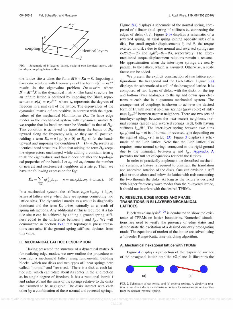
Figure 2(a) displays a schematic of the normal spring, com-

posed of a linear axial spring of stiffness kN connecting the

edges of disks (i, j). Figure 2(b) displays a schematic of a

reversed spring, an axial spring joining opposite sides of a

disk. For small angular displacements hi and hj, the torque

exerted on disk i due to the normal and reversed springs are

kNR2(hj� hi) and kRR2(�hj� hi), respectively. The afore-

mentioned torque-displacement relations remain a reasona-

ble approximation when the inter-layer springs are nearly

parallel to the lattice, which is assumed. Otherwise, a scale

factor can be added.

We present the explicit construction of two lattice con-

figurations: the hexagonal and the Lieb lattice. Figure 3(a)

displays the schematic of a cell of the hexagonal lattice. It is

composed of two layers of disks, with the disks on the top

and bottom layer analogous to the up and down spin elec-

trons at each site in a quantum mechanical system. The

arrangement of couplings is chosen to achieve the desired

form of D, with normal in-plane springs (gray color) of stiff-

ness knn/R2 between nearest neighbors. There are two sets of

interlayer springs between the next-nearest neighbors, nor-

mal springs (green) and reversed springs (red), both having

stiffness kiso/R2. The inter-layer spring between two sites

(p, l) and (q,�l) is of normal or reversed type depending on

the sign of lðnpq � ezÞ in Eq. (3). Figure 3 displays a sche-

matic of the Lieb lattice. Note that the Lieb lattice also

requires some normal springs connected to the rigid ground

due to the mismatch between g and kpp. Appendix A

provides the full set of equations for both the lattices.

In order to practically implement the described mechani-

cal systems, a fixture is required to constrain the translation

and undesired rotation of the disks. One can envision a stiff

plate or truss above and below the lattice with rods connecting

the two through the disks. As long as the fixture is designed

with higher frequency wave modes than the bi-layered lattice,

it should not interfere with the desired TPBMs.

IV. RESULTS: EDGE MODES AND PHASETRANSITIONS IN BI-LAYERED MECHANICALLATTICES

Bloch wave analysis24–26 is conducted to show the exis-

tence of TPBMs on lattice boundaries. Numerical simula-

tions are used to verify the presence of edge states and

demonstrate the excitation of a desired one-way propagating

mode. The equations of motion of the lattice are solved using

a 4th-order Runge-Kutta time-marching algorithm.

A. Mechanical hexagonal lattice with TPBMs

Figure 4 displays a projection of the dispersion surface

of the hexagonal lattice onto the xX-plane. It illustrates the

FIG. 1. Schematic of bi-layered lattice, made of two identical layers, with

interlayer coupling between them.

FIG. 2. Schematic of (a) normal and (b) reverse springs. A clockwise rota-

tion in one disk induces a clockwise (counter-clockwise) torque on the other

from the normal (reverse) spring.

084305-3 Pal, Schaeffer, and Ruzzene J. Appl. Phys. 119, 084305 (2016)

Reuse of AIP Publishing content is subject to the terms at: https://publishing.aip.org/authors/rights-and-permissions. Download to IP: 143.215.23.174 On: Mon, 20 Jun 2016

02:10:39

progression from a structure with no bandgap to one with a

topologically nontrivial bulk band gap that exhibits TPBMs.

The wavenumber along x, jx, is normalized by the lattice

vector magnitude d ¼ jd1j ¼ jd2j and p for viewing

convenience, and X¼x/x0 where x20 ¼ knn=I. Figures 4(a)

and 4(b) are dispersion relations for a 2D, periodic lattice

defined by the unit cell in Fig. 3(a), which approximate the

behavior of a lattice far from its boundaries. Figure 4(a)

shows the dispersion relation of an uncoupled bilayer system

with knn¼ 1 and kiso¼ 0. It consists of two identical disper-

sion surfaces superimposed. If kiso is instead 0.2, a topologi-

cally nontrivial bandgap opens up in the coupled bi-layered

system (Fig. 4(b)), so waves at frequencies X� 1.7 to 2.3

cannot propagate in the bulk of the lattice, i.e., far from the

boundaries. This is referred to as the “bulk bandgap.”9 Also

note that low frequency waves can no longer propagate and

there is a band gap at low frequencies due to the presence of

both normal and reverse springs. Note that reverse springs

prevent zero frequency modes at zero wavenumber. To

observe this, consider a chain of disks connected by reverse

springs. The equation of motion of disk i is I€hi þ kRR2ð2hi þhiþ1 þ hi�1Þ ¼ 0 and the dispersion relation of the system is

x ¼ 2j cosðkL=2Þj. They allow low frequency waves only at

k close to p. On the other hand, a chain of disks connected

by normal springs have dispersion relation x ¼ 2j sinðkL=2Þjand they do not permit low frequency waves close to p.

Hence, a combination of these normal and reverse leads to a

complete band gap at low frequencies.

Bloch wave analysis is performed on a strip of the hex-

agonal lattice to analyze the wave modes localized on the lat-

tice boundaries11,13 (see Appendix B for details). The disks

at each end of the strip are fixed. Figure 4(c) displays the

band diagram, showing 2 boundary modes spanning the bulk

bandgap. Note that there are actually 4 modes as each mode

superimposes another mode. On each boundary, there are 2

modes, propagating in opposite directions and they have dif-

ferent polarizations.20 Thus, an edge excited with a polariza-

tion corresponding to a boundary mode will have a wave

propagating in only one direction along the boundary.

Numerical simulations are performed to demonstrate the

excitation of a TPBM on a finite structure. The hexagonal

lattice unit cell is tessellated into a 20� 20 cell lattice and

the outer layer of cells is fixed. One site is excited such

that the torque is T" ¼ cos ðXsÞ and T# ¼ sin ðXsÞ on the top

and bottom layer, respectively, where time t is normalized

by defining s¼ tx0. A Hanning window is applied to T" and

T# so only 60 cycles of forcing are applied, and X¼ 2. The

FIG. 3. Hexagonal and Lieb lattice, respectively, (a) and (b) unit cell defined

by the lattice vectors d1 and d2 with nearest-neighbor interactions in gray, (c)

and (d) trimetric view, and (e) and (f) top view. (c)–(f) Bars represent axial

springs and the only DOF of each blue cylinder is rotation about its longitudi-

nal axis. Gray bars act within one layer. Red and green bars couple the layers.

FIG. 4. Bulk band structure of hexago-

nal lattice with (a) kiso¼ 0, (b)

kiso¼ 0.2, and (c) band diagram of a

periodic strip with fixed ends and

kiso¼ 0.2 coupling.

084305-4 Pal, Schaeffer, and Ruzzene J. Appl. Phys. 119, 084305 (2016)

Reuse of AIP Publishing content is subject to the terms at: https://publishing.aip.org/authors/rights-and-permissions. Download to IP: 143.215.23.174 On: Mon, 20 Jun 2016

02:10:39

result is plotted in Figs. 5(a)–5(d) for different moments in

the simulation. The coloring of each site corresponds to the

root mean square (RMS) of the displacement at that site,

considering the disks in both the top and bottom layer. The

simulations show that only one wave mode is excited, which

propagates in a clockwise direction around the structure, and

that this wave mode passes around the two corner types on

the lattice boundary without back-scattering. The displace-

ment magnitude is also seen to decay quickly with increasing

distance from the boundary. There is little dispersion given

the relatively constant slope for the edge mode at X¼ 2, so

the variation of the amplitude along the boundary is primar-

ily due to the windowing of the excitation.

If the excitation to the lattice is modified so that

T# ¼ �sinðXsÞ but T" remains the same, only the wave

mode which propagates counter-clockwise around the lattice

is excited (Figs. 5(e)–5(h)). Thus, the direction of energy

propagation can be selected via the polarization of the input

to the system.

B. Mechanical Lieb lattice with TPBMs

Our final example studies the Lieb lattice. The bulk dis-

persion surface of the mechanical Lieb lattice with knn¼ 1

and kiso¼ 0 is pictured in Fig. 6(a), projected on the xX-

plane with the wavenumber jx normalized as in Subsection

IV A. Low frequency waves cannot propagate, due to the

presence of ground springs. The addition of inter layer cou-

pling with kiso¼ 0.2 opens two bandgaps spanning X� 2.0

to 2.2 and X� 2.2 to 2.4.

A strip of the Lieb lattice is analyzed in the same way as

the hexagonal lattice, with the disks at the boundary fixed.

Note that there are two types of edges arising in the Bloch

analysis of a strip. The first edge corresponds to the edge of a

unit cell closer to the x-axis in the schematic in Fig. 3(b),

while the second type corresponds to the opposite edge of

the unit cell. Figure 6(c) displays the corresponding disper-

sion diagram. There are 4 distinct modes localized at the

boundary which span the bulk bandgaps. They correspond to

the left and right propagating modes on the two distinct

boundaries.

For numerical simulations, first a lattice is considered with

all boundaries identical. The edge described by the upper end

of the strip, i.e., positive y in Fig. 3(b), is used to demonstrate

the excitation of a TPBM in a simulation of the Lieb lattice.

The unit cell in Fig. 3(d) is tessellated into a lattice of 30� 30

unit cells and lattice sites are added at the required edges to

make all the boundaries identical. Then, the outer layer of cells

is fixed. The same forcing input as for the hexagonal lattice is

used except X¼ 2.1. With T" ¼ cos ðXsÞ and T# ¼ sin ðXsÞ, a

clockwise-propagating mode is excited, but if T# ¼ �sin ðXsÞ,a counter-clockwise propagating wave is excited. Figures

7(a)–7(c) depict the results, and the waves are seen to transi-

tion between edges without reflections.

Next, we present numerical simulations of a wave prop-

agating from one boundary type to another (Figs. 7(d)–7(f)).

The same forcing input is used as in the aforementioned sim-

ulation, and the simulation domain is a 30� 30 cell lattice

with the outer layer of cells fixed. The wave packet propa-

gates on both edge types at different velocities and exhibits

no back-scattering when transitioning from one edge to the

other. In Figs. 7(e) and 7(f), the wave packet looks smaller

than in Figs. 7(a)–7(c) because the “smooth” edge type is not

as dispersive as the other, and the wave has not had as much

FIG. 5. RMS displacement at each lattice site for different moments in time

s. (a)–(d) Clockwise propagation. (e)–(h) Counter-clockwise propagation.

Red denotes the greatest displacement and green denotes none.

FIG. 6. Bulk band structure of Lieb

lattice with (a) kiso¼ 0, (b) kiso¼ 0.2,

and (c) band diagram of a periodic

strip with fixed ends and kiso¼ 0.2

coupling.

084305-5 Pal, Schaeffer, and Ruzzene J. Appl. Phys. 119, 084305 (2016)

Reuse of AIP Publishing content is subject to the terms at: https://publishing.aip.org/authors/rights-and-permissions. Download to IP: 143.215.23.174 On: Mon, 20 Jun 2016

02:10:39

time to disperse. Indeed, this behavior is consistent with the

trends observed in the band diagram, where there are two

group velocities at each frequency in the bulk bandgap

region. Each mode corresponds to a localized wave on a par-

ticular boundary type and they are all unidirectional. As the

wave traverses from one boundary type to the other, there is

thus a change in group velocity as the wave transitions from

one branch to another.

C. Topological phase transitions by varying groundspring stiffness

We finally discuss the effect of ground springs on the

band structure. We label the sites having 4 and 2 nearest

neighbors by indices 1 and 2, respectively. There are two

sets of ground springs, kg1 and kg2 connecting the site types 1

and 2 with the ground, respectively. As mentioned earlier,

modifying both the ground springs by the same amount has

the effect of translating the entire band along the frequency

axis without altering their topology. The values of ground

springs which correspond to a flat band, an exact analogue of

the quantum mechanical case, satisfy the constraint

kg1� kg2¼ 2knn� 4kiso. We thus vary kg2 keeping kg1 fixed

and observe the effect on the band structure by computing

the spin Chern numbers.7,27 The Chern numbers Cþ and C�of the top and bottom bands related as Cþ¼�C� and the

spin Chern number is given by Cs¼Cþ�C�. Figure 8 illus-

trates the phase diagram of the system as a function of the

relative ground stiffness and the interlayer coupling stiffness.

These stiffness values are normalized by the in-plane stiff-

ness knn.

There are three regions (I, II, and III) in the phase dia-

gram, with phase boundaries between them. The central

region (I) has TPBMs between the lower and the upper bands

and is topologically equivalent to the case studied earlier

having a flat band at the center. The bands have spin Chern

number Cs¼ (�2, 0, 2). The region on the left (III) has

TPBMs only between the middle band and the lower band,

while the region on the right (II) has TPBMs between the top

and middle bands. These regions have spin Chern numbers

Cs¼ (�2, 2, 0) and (0, �2, 2), respectively. Indeed, the

change in band topology is reflected in the change in their

respective Chern numbers. Thus, the presence of edge modes

is insensitive to small changes in the ground springs, as long

as they remain within the phase boundaries, thereby illustrat-

ing the robustness to imperfections in material properties. It

also shows the parameter space over which these TPBMs

can be achieved and provides guidelines for designing latti-

ces. Figure 8 illustrates the band diagrams at each of the

phases. In these calculations, the interlayer spring stiffness is

fixed at kiso¼ 0.1, while the relative strengths of the ground

springs is varied so that kg2� kg1� (2� 4kiso) takes values

{0, 0.5,�0.5} in Figs. 8(b)–8(d). Note that as the ground

stiffness deviates from the value kg2� kg1¼ 2� 4kiso, the

center band is not flat anymore. The center band grows and

touches either the top or the lower band depending on the

value of kg2� kg1, at which point a phase transition occurs.

To observe this phase transition from the structure of the

dynamical matrix, we apply the inverse transform ðH ¼UDHU†Þ to a lattice with arbitrary ground springs to recover

the equivalent quantum Hamiltonian. This transform simpli-

fies the eigenvalue analysis as the top and bottom layers are

effectively decoupled. Applying Bloch reduction on a unit

cell results in the characteristic equation ða� kg2 þ kg1 þ 2

�4kisoÞða2 � 16k2isoÞ ¼ 0 for the eigenvalues a at the point

jx¼ jy¼ p/2. A topological phase transition occurs only

when the bands touch, i.e., when there are degenerate eigen-

values. Indeed, these degenerate values arise when a¼ kg2

� kg1� 2þ 4kiso¼64kiso, which are the phase transition

boundaries in Fig. 8. We finally remark on the tunability of

our lattices by varying the ground springs. These phase tran-

sitions give a way to modify the behavior of the lattice at a

particular frequency from unidirectional propagation along

FIG. 7. RMS displacement at each lattice site for different moments in time

s. (a)–(c) Clockwise propagation with one edge type. (d)–(f) Clockwise

propagation with two edge types. Red denotes the greatest displacement and

green denotes none.FIG. 8. (a) Phase diagram with ground spring and interlayer spring stiffness

parameters, showing three distinct topological phases. (b)–(d) Close-up

view of band diagrams corresponding to each of the phases.

084305-6 Pal, Schaeffer, and Ruzzene J. Appl. Phys. 119, 084305 (2016)

Reuse of AIP Publishing content is subject to the terms at: https://publishing.aip.org/authors/rights-and-permissions. Download to IP: 143.215.23.174 On: Mon, 20 Jun 2016

02:10:39

the edge to bulk modes to no propagation along the edges

and the interior.

V. CONCLUSIONS

A framework for generating a family of mechanical sys-

tems that exhibit TPBMs is derived and demonstrated

numerically. A mechanical analogue of a quantum mechani-

cal system that exhibits edge modes is obtained by an appro-

priate transformation and this analogue defines the lattice

network topology. The phase boundaries of the topological

phase in the vicinity of the parameters defining the mechani-

cal analogue are demonstrated to show the robustness to

mechanical imperfections. The hexagonal and Lieb lattice

examples show the efficacy of the methodology and numeri-

cal simulations reinforce it. Excitation polarization is shown

to determine the direction of energy propagation. The Lieb

lattice is used to highlight that the type of edge influences

the boundary wave propagation. Finally, topological phase

transitions are obtained by modifying the ground springs,

thereby illustrating the potential for tunable wave propaga-

tion in these lattices. Future work entails extension of these

concepts to incorporate general mechanical elements.

ACKNOWLEDGMENTS

This research was funded by a grant from the Air Force

Office of Scientific Research (AFOSR) Grant No. FA9550-

13-1-0122.

APPENDIX A: EQUATIONS OF MOTION

We present the complete equations of motion for the disks

in a unit cell for both the lattices considered in this work.

Consider an infinite lattice divided into unit cells, and each unit

cell is indexed by a pair of integers (i, j), denoting its location

with respect to a fixed coordinate system. Let I be the rotational

inertia of each disk and let ha;bi;j denote the angular displacement

of a disk. The two subscripts (i, j) identify the unit cell and the

two superscripts identify the location of the disk within the unit

cell (i, j). The first superscript index denotes its location in the

xy-plane, while the second superscript index denotes whether

the disk is in top (t) or bottom (b) layer.

1. Hexagonal lattice

Figure 9 displays the top layer of a unit cell of the hexago-

nal lattice. Each layer has two disks, indexed as illustrated.

The equations of motion of the four disks of the unit cell are

I€h1;t

i;j ¼ knnðh2;ti;j þ h2;t

i;j�1 þ h2;ti�1;j � 3h1;t

i;j Þ � 6kisoh1;ti;j

þ kisoðh1;biþ1;j þ h1;b

i�1;jþ1 þ h1;bi;j�1Þ

� kisoðh1;bi;jþ1 þ h1;b

i�1;j þ h1;biþ1;j�1Þ; (A1a)

I€h2;t

i;j ¼ knnðh1;ti;j þ h1;t

i;jþ1 þ h1;tiþ1;j � 3h2;t

i;j Þ � 6kisoh2;ti;j

þ kisoðh2;bi;jþ1 þ h2;b

i�1;j þ h2;biþ1;j�1Þ

� kisoðh2;biþ1;j þ h2;b

i�1;jþ1 þ h2;bi;j�1Þ; (A1b)

I€h1;b

i;j ¼ knnðh2;bi;j þ h2;b

i;j�1 þ h2;bi�1;j � 3h1;b

i;j Þ � 6kisoh1;bi;j

þ kisoðh1;tiþ1;j þ h1;t

i�1;jþ1 þ h1;ti;j�1Þ

� kisoðh1;ti;jþ1 þ h1;t

i�1;j þ h1;tiþ1;j�1Þ; (A1c)

I€h2;b

i;j ¼ knnðh1;bi;j þ h1;b

i;jþ1 þ h1;biþ1;j � 3h2;b

i;j Þ � 6kisoh2;bi;j

þ kisoðh2;ti;jþ1 þ h2;t

i�1;j þ h2;tiþ1;j�1Þ

� kisoðh2;tiþ1;j þ h2;t

i�1;jþ1 þ h2;ti;j�1Þ: (A1d)

2. Lieb lattice

Figure 10 displays the top layer of a unit cell of the Lieb

lattice. Each layer has three disks, indexed as illustrated. Let

kg ¼ maxð2knn þ 4kiso; 4knnÞ be the additional term required

to shift all the bands upward. The equations of motion of the

six disks of the unit cell are

I€h1;t

i;j ¼ knnðh2;ti;j þ h3;t

i;j þ h3;ti;j�1 þ h2;t

i�1;jÞ � kgh1;ti;j ; (A2a)

I€h2;t

i;j ¼ knnðh1;ti;j þ h1;t

iþ1;jÞ � kgh2;ti;j

þ kisoðh3;biþ1;j � h3;b

i;j þ h3;bi;j�1 � h3;b

iþ1;j�1Þ; (A2b)

I€h3;t

i;j ¼ knnðh1;ti;j þ h1;t

i;jþ1Þ � kgh3;ti;j

þ kisoðh2;bi�1;jþ1 � h2;b

i�1;j þ h2;bi;j � h2;b

i;jþ1Þ; (A2c)

I€h1;b

i;j ¼ knnðh2;bi;j þ h3;b

i;j þ h3;bi;j�1 þ h2;b

i�1;jÞ � kgh1;bi;j ; (A2d)

I€h2;b

i;j ¼ knnðh1;bi;j þ h1;b

iþ1;jÞ � kgh2;bi;j

þ kisoðh3;tiþ1;j � h3;t

i;j þ h3;ti;j�1 � h3;t

iþ1;j�1Þ; (A2e)

FIG. 9. Schematic of a hexagonal unit cell. The top layer is shown, along

with index of the disks.

FIG. 10. Schematic of a Lieb lattice unit cell. The top layer is shown, along

with index of the disks.

084305-7 Pal, Schaeffer, and Ruzzene J. Appl. Phys. 119, 084305 (2016)

Reuse of AIP Publishing content is subject to the terms at: https://publishing.aip.org/authors/rights-and-permissions. Download to IP: 143.215.23.174 On: Mon, 20 Jun 2016

02:10:39

I€h3;b

i;j ¼ knnðh1;bi;j þ h1;b

i;jþ1Þ � kgh3;bi;j

þ kisoðh2;ti�1;jþ1 � h2;t

i�1;j þ h2;ti;j � h2;t

i;jþ1Þ: (A2f)

Note that the disks indexed 1 and {2, 3} have different

number of neighbors and hence ground springs are required

to ensure that all the bands are shifted by the same amount.

The ground stiffness is required on either the 1 disks or on

the {2, 3} depending on the relative magnitudes of knn and

kiso. Its value is 4kiso� 2knn on disk 1 if 2kiso> knn or

2knn� 4kiso on disks {2, 3} in each unit cell.

APPENDIX B: BLOCH WAVE ANALYSIS OF A STRIP

A convenient way to check for the existence of TPBMs

is to calculate the band diagram for the 1D, periodic system

created in the following way. The unit cell is tessellated a fi-

nite number of times along one lattice vector to make a strip,

and then made periodic along the other lattice vector. The

result is a system with two parallel boundaries. TPBMs, if

they exist in a specific structure, will manifest in the fre-

quency range of the bulk bandgap due to the bulk-edge cor-

respondence principle.28,29 Furthermore, the deformation

associated with these modes, i.e., the eigenvectors, will be

localized at one of the boundaries. Indeed, there is some re-

dundancy in solving for edge modes this way, as an infinite

half space would describe only one edge. However, this

method requires only a small modification from a 2D Bloch

analysis implementation and is therefore quite convenient

and practical.

For the results shown in this article, a strip of the hexag-

onal lattice is made by repeating 27 unit cells along d1 and

then made periodic along d2 by assuming the traveling wave

solution. The disks of the unit cells at each end of the strip

are rigidly fixed, so there are 25 unit cells elastically con-

nected to two rigid “walls.” Similarly, to analyze another

type of edge, the ends of the strip can be left free. For the

Lieb lattice, the strip is also made by repeating 27 unit cells

(Fig. 3(b)) along d1, rigidly fixing the unit cells at each end

of the strip, and making the strip periodic along d2.

1F. D. M. Haldane, “Model for a quantum Hall effect without landau levels:

Condensed-matter realization of the “parity anomaly”,” Phys. Rev. Lett.

61(18), 2015 (1988).2Y. Zhang, Y. W. Tan, H. L. Stormer, and P. Kim, “Experimental observa-

tion of the quantum Hall effect and Berry’s phase in graphene,” Nature

438(7065), 201–204 (2005).3C. L. Kane and E. J. Mele, “Quantum spin Hall effect in graphene,” Phys.

Rev. Lett. 95(22), 226801 (2005).4C. L. Kane and E. J. Mele, “Z2 topological order and the quantum spin

Hall effect,” Phys. Rev. Lett. 95(14), 146802 (2005).

5B. A. Bernevig, T. L. Hughes, and S. C. Zhang, “Quantum spin Hall effect

and topological phase transition in HgTe quantum wells,” Science

314(5806), 1757–1761 (2006).6N. Goldman, W. Beugeling, and C. M. Smith, “Topological phase transi-

tions between chiral and helical spin textures in a lattice with spin-orbit

coupling and a magnetic field,” Europhys. Lett. 97(2), 23003 (2012).7W. Beugeling, N. Goldman, and C. M. Smith, “Topological phases in a

two-dimensional lattice: Magnetic field versus spin-orbit coupling,” Phys.

Rev. B 86(7), 075118 (2012).8F. D. M. Haldane and S. Raghu, “Possible realization of directional optical

waveguides in photonic crystals with broken time-reversal symmetry,”

Phys. Rev. Lett. 100(1), 013904 (2008).9L. Lu, J. D. Joannopoulos, and M. Soljacic, “Topological photonics,” Nat.

Photonics 8, 821–829 (2014).10V. Peano, C. Brendel, M. Schmidt, and F. Marquardt, “Topological phases

of sound and light,” Phys. Rev. X 5(3), 031011 (2015).11E. Prodan and C. Prodan, “Topological phonon modes and their role in

dynamic instability of microtubules,” Phys. Rev. Lett. 103(24), 248101

(2009).12L. Zhang, J. Ren, J. S. Wang, and B. Li, “Topological nature of the phonon

Hall effect,” Phys. Rev. Lett. 105(22), 225901 (2010).13P. Wang, L. Lu, and K. Bertoldi, “Topological phononic crystals with one-

way elastic edge waves,” Phys. Rev. Lett. 115, 104302 (2015).14T. Kariyado and Y. Hatsugai, “Manipulation of Dirac cones in mechanical

graphene,” Sci. Rep. 5, 18107 (2015).15A. B. Khanikaev, R. Fleury, S. H. Mousavi, and A. Al�u, “Topologically ro-

bust sound propagation in an angular-momentum-biased graphene-like res-

onator lattice,” Nat. Commun. 6, 8260 (2015).16R. Fleury, A. Khanikaev, and A. Alu, “Floquet topological insulators for

sound,” preprint arXiv:1511.08427 (2015).17Z. Yang, F. Gao, X. Shi, X. Lin, Z. Gao, Y. Chong, and B. Zhang,

“Topological acoustics,” Phys. Rev. Lett. 114(11), 114301 (2015).18N. Swinteck, S. Matsuo, K. Runge, J. O. Vasseur, P. Lucas, and P. A.

Deymier, “Bulk elastic waves with unidirectional backscattering-immune

topological states in a time-dependent superlattice,” J. Appl. Phys. 118(6),

063103 (2015).19G. Salerno, T. Ozawa, H. M. Price, and I. Carusotto, “Floquet topological

system based on frequency-modulated classical coupled harmonic oscil-

lators,” Phys. Rev. B 93(8), 085105 (2016).20R. S€usstrunk and S. D. Huber, “Observation of phononic helical edge

states in a mechanical ‘topological insulator’,” Science 349(6243), 47–50

(2015).21M. Xiao, W. J. Chen, W. Y. He, and C. T. Chan, “Synthetic gauge flux

and Weyl points in acoustic systems,” Nat. Phys. 11, 920 (2015).22P. A. Deymier, K. Runge, N. Swinteck, and K. Muralidharan, “Torsional

topology and fermion-like behavior of elastic waves in phononic

structures,” C. R. M�ec. 343(12), 700–711 (2015).23S. H. Mousavi, A. B. Khanikaev, and Z. Wang, “Topologically protected

elastic waves in phononic metamaterials,” Nat. Commun. 6, 8682 (2015).24F. Bloch, “€Uber die quantenmechanik der elektronen in kristallgittern,” Z.

Phys. 52(7–8), 555–600 (1929).25L. Brillouin, Wave Propagation in Periodic Structures: Electric Filters

and Crystal Lattices (Dover Publications, Inc., 1953).26M. I. Hussein, M. J. Leamy, and M. Ruzzene, “Dynamics of phononic

materials and structures: Historical origins, recent progress, and future out-

look,” Appl. Mech. Rev. 66(4), 040802 (2014).27T. Fukui, Y. Hatsugai, and H. Suzuki, “Chern numbers in discretized

Brillouin zone: Efficient method of computing (spin) Hall conductances,”

J. Phys. Soc. Jpn. 74(6), 1674–1677 (2005).28R. Jackiw and C. Rebbi, “Solitons with fermion number 1/2,” Phys. Rev.

D 13(12), 3398 (1976).29M. Z. Hasan and C. L. Kane, “Colloquium: Topological insulators,” Rev.

Mod. Phys. 82(4), 3045 (2010).

084305-8 Pal, Schaeffer, and Ruzzene J. Appl. Phys. 119, 084305 (2016)

Reuse of AIP Publishing content is subject to the terms at: https://publishing.aip.org/authors/rights-and-permissions. Download to IP: 143.215.23.174 On: Mon, 20 Jun 2016

02:10:39