Helical 'Automatic 'of Helicopte'rs With Microwave Landing · Helical 'Automatic 'of Helicopte'rs...

NASA TP 2 109 c.1 I

,J ."

' .I

. .

-' NASA ,Technical Paper-- 21 09

f December 1982 -

Helical 'Automatic 'of Helicopte'rs With Microwave Landing

\ I .

John D. Foster, Leonard A. McGee, and Daniel C . Dugan

I

https://ntrs.nasa.gov/search.jsp?R=19830010433 2018-07-03T08:12:29+00:00Z

TECH LIBRARY KAFB, NM

NASA Technical Paper 21 09

1982

National Aeronautics and Space Administration

Scientific and Technical Information Branch

00bB3bL

Helical Automatic Amroaches of Helicopters With Microwave Landing Systems

A &

John D. Foster, Leonard A. McGee, and Daniel C. Dugan Ames Research Center Moffett Field, California

ACRONYMS

AGL

DME

I F R

I L S

IMC

IMU

INS

MLS

TACAN

VOR

VORTAC

above ground level

distance measuring equipment

instrument flight rules

instrument landing system

instrument meteorological conditions

inertial measurement unit

inertial navigation system

microwave landing system

tactical air navigation aid

very high frequency omni range navigation aid

a co-located VOR and TACAN facility

iii

HELICAL AUTOMATIC APPROACHES OF HELICOPTERS WITH MICROWAVE LANDING SYSTEMS

John D. Foster, Leonard A. McGee, and Daniel C. Dugan

Ames Research Center

SUMMARY

A program is under way at Ames Research Center to develop a data base for estab- lishing navigation and guidance concepts for all-weather operation of rotorcraft. One of the objectives is to examine the feasibility of conducting simultaneous rotorcraft and conventional fixed-wing, noninterfering, landing operations in instrument meteorological conditions (IMC) at airports equipped with microwave landing systems (MLSs) for fixed-wing traffic.

One way to accomplish this objective is to have rotorcraft fly spiral approach paths in airspace separate from that of the fixed-wing traffic. Rotorcraft instrument-flight-rules (IFR) approaches could use the airspace along the edge of the MLS lateral coverage, which would allow complete separation from fixed-wing traffic.

An initial test program to investigate the feasibility of conducting automatic helical approaches was completed, using the MLS at Crows Landing near Ames. These tests were flown on board a UH-1H helicopter equipped with a digital automatic landing system. A total of 48 automatic approaches and landings were flown along a two-turn helical descent, tangent to the centerline of the MLS-equipped runway to determine helical flight performance and to provide a data base for comparison with future flights for which the helical approach path will be located near the edge of the MLS coverage. In addition, 13 straight-in approaches were conducted. The performance with varying levels of state-estimation system sophistication was evaluated as part of the flight tests. The results indicate that helical approaches to MLS-equipped runways are feasible for rotorcraft and that the best position accuracy was obtained using the Kalman-filter state-estimation with inertial navigation systems (INS) sensors.

INTRODUCTION

As rotorcraft assume a greater role in the Nation's transportation system, the need for rotorcraft instrument-flight-rules (IFR) operations in high-traffic density terminal areas will increase, aggravating the existing air-traffic control problems of mixing low-speed traffic with high-speed jet transport traffic. The efficiency and convenience of the rotorcraft as a feeder to major airports for corporate and commercial travelers will be diminished if time and fuel are wasted waiting for spacing between arriving and departing fixed-wing traffic. Therefore, in high-density traffic terminals it will be necessary to separate rotorcraft and fixed-wing traffic by assigning them to adjacent airspace for all-weather conditions. With this separation, the problems of aircraft spacing and traffic conflict would be limited to vehicles with similar approach and departure speeds, thus simplifying the air-traffic control problem.

As indicated in reference 1, a promising way to provide airspace separation is to use a helical approach for the rotorcraft traffic. A helical descent allows the vehicle to lose altitude in a confined airspace without descending along a steep

glide slope at very low airspeeds. This also avoids the poor helicopter handling qualities associated with steep descents. The helix can be located in a vacant airspace sector of the airport, with the rotorcraft entering above the fixed-wing approach and departure corridors in the immediate airport vicinity.

A major constraint on the choice of rotorcraft landing approach airspace is the coverage limit of the landing-approach navigation aid. It is anticipated that the precision airport approach aid will be the microwave landing system (MLS). This system provides significantly greater lateral and vertical coverages than does the current instrument landing system (ILS), making possible many separate approach paths to the same facility. Although separate MLS installations for rotorcraft and fixed-wing traffic may be provided at the airports with the highest traffic volume, many airports will use only a single MLS. This latter situation imposes a greater constraint in choosing the rotorcraft approach airspace. The helix must be within the lateral and vertical MLS coverage limits of the MLS azimuth signal, yet displaced sufficiently from the fixed-wing runway to allow simultaneous approaches. The helix need not lie within the coverage provided by the MLS elevation signal.

To investigate the feasibility of this airspace separation, Ames Research Center has a flight-research program under way to study operational procedures, guidance, and navigation requirements for making automatic helicopter approaches and landings along helical approach paths, using an MLS for fixed-wing traffic. Flight experiments were conducted using a NASA/Army UH-1H helicopter equipped with a digital flight- guidance system called V/STOLAND. This versatile, integrated system has many fea- tures, one of which is the capability for coupled, automatic approaches to hover and touchdown while using VORTAC, TACAN, and MLS information, either separately or in combination.

This initial investigation consisted of 48 automatic approaches to touchdown along a two-turn helix, tangent to the centerline of the MLS-equipped runway. This location was chosen to provide a data base for comparison with future flight tests in which the helical approach path will be located at the edge of the MLS coverage, as well as to simplify the pilot's task of visually monitoring the approach during the development and checkout of the flight guidance system. In addition, 13 straight-in approaches were flown to enlarge the data base and to assess the helical approach on vehicle state-estimation and guidance performance.

Among other parameters investigated, the performance with three levels of state- estimation sophistication was evaluated in these flight tests. The three included a Kalman filter, using INS platform inertial sensors; a Kalman filter, using body- mounted inertial sensors; and a complementary filter, using body-mounted inertial sensors.

Specific objectives of these flight tests were to (1) determine helical approach airspace requirements; (2) compare helical approach performance with three different levels of state-estimation sophistication; ( 3 ) determine tracking precision at the conventional takeoff and landing (CTOL) Category I1 decision height window; ( 4 ) determine precision of decelerating to a hover over a helipad; (5) measure MLS azimuth distance-measuring-equipment (DME) errors; and (6) determine pilot opinion of automatic helical approach performance.

This report documents the overall system performance obtained in these flight tests, as well as the guidance, translational state estimation, and control performance achieved while flying automatic, helical approaches.

2

GUIDANCE, TRANSLATIONAL STATE-ESTIMATION, AND CONTROL SYSTEM DESCRIPTION

System Concept

V/STOLAND is an automatic, flight guidance system capable of conventional autopilot tasks such as altitude and airspeed hold, en route navigation-aid capture and track, three-dimensional area-navigation, and coupled automatic approach and landing. En route navigation can use either VORTAC or TACAN for horizontal measurements and a barometric altimeter for vertical measurements; the area-navigation modes can also use the MLS. The approach and landing modes use the MLS azimuth and range in the horizontal plane and the baroaltimeter, MLS elevation, and radar altimeter in the vertical plane.

This report is concerned only with the approach and landing flight phases; consequently, system modes not associated with these phases are not discussed. Reference 2 describes the total system and all individual modes. Only the guidance, state-estimation, and control functions for the automatic approach and landing modes are discussed here.

Guidance Functions

The guidance system has two main functions: (1) to use the estimated aircraft position from the state estimator to compute the approach flightpath that will take the aircraft from an initial approach fix to touchdown at the appropriate airspeeds; and ( 2 ) to compute aircraft pitch-attitude, roll-attitude, and vertical-speed commands to control the aircraft along the approach flightpath, without exceeding the aircraft operational limitations.

The landing approach path is defined in a right-hand Cartesian coordinate system located on the centerline of runway 35 at Crows Landing, Naval Auxiliary Landing Field (NALF), California (fig. 1). Each approach path ends at the touchdown point, shown in the figure at -914 m ( -3 ,000 ft) from the MLS glide-slope antenna, which is in the center of the circle called the helipad.

The helical approach shown in figure 2 begins with a constant-altitude segment, 762 m ( 2 , 5 0 0 ft) above ground level (AGL), along the runway centerline extension. The helix is tangent to this segment, 984 m ( 3 , 0 0 0 ft) from the touchdown point with a radius of 530 m ( 1 , 7 3 8 ft). The flightpath follows a -6.11" glide, originating at the tangent point, around the helix twice to a 2.5" glide slope aimed at the touchdown point, as shown in figure 3 . The aircraft follows this glide slope to a height of 4 . 6 m ( 1 5 ft), where it remains until reaching the hover point. The last segment is the vertical letdown to touchdown.

The straight-in approach path begins with a constant-altitude segment, 610 m (2,000 ft) above the touchdown point elevation, along the runway centerline extension. It intercepts and follows a 10" glide slope aimed at a ground-intercept point at 458 m ( 1 , 5 0 3 ft) from touchdown, the same location as the helix glide slope ground- intercept point. The final straight-in approach geometry, also shown in figure 3 , is the same as in the helical approach, except that the 2.5" glide slope intercept is somewhat closer to the touchdown point.

The airspeed profile (fig. 3(b)) is the same for the helical and straight-in approaches. The airspeed command is set for 31 m/sec (60 knots) for the entire

3

approach up to the flare. During the flare, the aircraft ground speed follows a constant-g deceleration profile that brings the aircraft to hover over the desired touchdown point. The final approach path geometry and the flare deceleration profile were designed to keep the aircraft from violating the height-velocity restriction of the UH-1H single-engine helicopter.

Details of the guidance laws for the landing approach, including the airspeed profile for the flare, are presented in appendix A .

Control Functions

Each of the helicopter controls (longitudinal cyclic, lateral cyclic, collective, and tail-rotor blade pitch) is driven by series and parallel servos that move in response to commands from the stabilization and control equations mechanized in the basic computer. The series servos are electrohydraulic position servos that produce additive position changes in control linkages that are not reflected in the pilot's stick or pedal positions. The parallel servos are electromechanical rate servos that act on the stick and pedals to off-load the series servos. Longitudinal cyclic controls pitch attitude; lateral cyclic controls roll attitude; and collective controls vertical speed. Tail-rotor pitch is not controlled by a guidance steering command; it functions to maintain zero lateral body acceleration for airspeeds greater than 19 m/sec (37 knots). For speeds less than 19 m/sec ( 3 7 knots), the tail-rotor control maintains aircraft heading. Control-system equations, hardware mechanization, and other details are given in reference 2.

State-Estimator Functions

The ability of an automatic landing system to follow an approach path precisely requires an accurate estimate of the vehicle state (position and velocity). Aircraft position measurements with bias errors and high-frequency random noise are common to most state-of-the-art ground navigation aids and associated airborne receivers. The function of the airborne state-estimator system was to provide smoothed estimates of the aircraft position and velocity by using various filters. Three filters were tested during this flight-test program.

In the first and most sophisticated method, a Kalman filter, described in appendix B y was used. Inertial accelerations from an LTN-51 inertial navigation system (INS), TACAN range and azimuth, and MLS range and azimuth were used for the horizontal estimates. For the vertical estimates, the signals that were used were barometric altitude from a static-pressure sensor, MLS elevation angle, and radar altitude. The Kalman filter consisted of two filters - an eight-state horizontal space filter and a three-state vertical filter. The eight horizontal states were x- and y-position errors, x- and y-velocity errors, x- and y-accelerations-bias errors, the TACAN range bias estimate, and the TACAN bearing bias estimate. Since the INS provided high-quality acceleration data, the acceleration uncertainty modeled in the filter was small. The three vertical states were z-position, z-velocity err01 estimates, and vertical acceleration bias error. When the aircraft was at an altitude greater than 122 m (400 ft) above the ground, the barometric altitude was the primary vertical measurement and the MLS elevation angle was used only to estimate the baro-altitude bias error. For altitudes less than 122 m (400 ft) above the ground, the radar altimeter provided the vertical-measurement to the filter.

4

In the second method, a Kalman filter was used that had a structure identical to that of the first filter, with the exception that the three components of acceleration were measured using body-mounsed accelerometers. These measurements were transformed through the aircraft attitude angles measured by the vertical and directional gyros to give the runway-coordinate accelerations that were processed by the filter. These accelerations were subject to greater errors than those measured in the INS platform, as a result of alignment errors between the attitude gyros and the body-mounted accelerometers. Vertical gyro precession during the turns in the helix introduced substantial additional time-varying errors in the computed acceleration. These acceleration errors usually resulted in low-frequency errors in the position and velocity estimates during the helical segment of the approach. To minimize these errors, the magnitude of acceleration uncertainty modeled in the filter had to be greater than in the previousicase wherein the accelerations were measured by an INS. In addition to increasing path-tracking dispersions, greater noise in the guidance commands caused greater control activity. Hence, when body-mounted inertial sensors were used, a compromise had to be made between control activity and navigation error. For this flight-test program, the modeled uncertainties in the acceleration errors were chosen to minimize control activity, especially when hovering, in order to avoid lateral and backward motion during touchdown. As a result, some accuracy in the state (position and velocity) estimates was sacrificed in the earlier portion of the approach.

In the third method, constant-gain complementary filters were used in place of the Kalman filter to blend the body-mounted inertial sensor data with the TACAN and MLS data (see appendix B for details). The runway-coordinate accelerations were derived from the same sensors and in the same manner as in the second method. In contrast to the other two methods, the complementary filters had three components that were basically independent. The significant difference between these filters and the Kalman filters was that the measurement gains were constant for a given navigation source and did not vary with the position relative to that source. There was one set of gains for TACAN measurements and one set for MLS measurements. The gains used for the flight test gave greater sensitivity to measurement noise than either of the Kalman filters. Consequently, this filter tended to reduce the effect of the low-frequency inertial errors at the expense of passing more measurement noise to the guidance commands. This reduction resulted in greater control activity.

EQUIPMENT DESCRIPTION

Aircraft

The flight-test aircraft was a UH-1H helicopter (fig. 4). The UH-1H has a maximum gross weight of 4,300 kg (9,460 lb) and a maximum airspeed of 63 m/sec (124 knots) at sea level. It is powered by a single, turboshaft, T53-L-13 engine. The flight controls for the UH-1H are hydraulically boosted, and rate damping is provided by a gyro bar. Hydraulic and electrical systems were modified to drive the flight-guidance equipment and servoactuators. In addition, special racks for the electronic equipment were installed aft of the pilot's seats. The fore and aft MLS antennas are also shown in figure 4 . An electronic device is used to select reception from the antenna with the greatest signal strength, which occurs when one antenna is shielded by the fuselage during the helical approach.

5

Flight-Guidance System

Major flight-guidance system components are shown in the block diagram in figure 5. Only a brief description of the major components is provided here; a detailed description is given in reference 2.

The central system component is the data adapter, which provides information transfer between the subsystems. It converts information into the proper signal format for input and output and provides multiplexed analog-to-digital, digital-to- digital, and digital-to-analog conversions.

The basic and research 1819B computers are general-purpose, airborne digital computers that use fixed-point arithmetic. Routine guidance, navigation, and control functions, along with supporting functions such as display generation and system monitoring, were programmed into the basic computer. Software associated with the Kalman navigation filters was programmed into the research computer.

The vehicle sensors provided measurements of the aircraft attitude, attitude rate, acceleration, and certain air-data parameters, such as airspeed, static pressure, and ambient temperature. The airspeed sensor and the static pressure port were located on the end of a 1.4-m (4.6-ft) boom mounted on the aircraft nose. The boom installation minimized the effects of small, main-rotor induced, side-slip angles on the true airspeed and static-pressure measurements. A more detailed description of the problem solution is given in appendix C.

The navigation aids included the radar altimeter, and the radio navigation receivers (VOR, TACAN, and MLS).

The pilot interacted with the flight-guidance system through the mode-select panel, the keyboard, and the multifunction display control panel. Pilot displays consisted of conventional electromechanical attitude-director indicator (ADI), horizontal situation indicator (HSI) instruments, and a cathode-ray tube display, labeled the multifunction display (MFD). The MFD provided position information in a moving- map format.

The guidance and control laws controlled the aircraft through the servo inter- lock unit (SIU). This unit contained the hardware necessary to drive the electrohydraulic series servos and the electromechanical parallel servos that are connected to the aircraft flight controls.

The data acquisition system collected digital data from the data adapter, converted analog vehicle sensor data to digital data, and sent this combination through a telemetry transmitter to a ground station to be recorded. The recorded data were processed after the flight to time-correlate them with the ground-tracking radar data; this resulted in a single recording with both the airborne and radar data. A detailed description of this process is given in reference 3 .

MEASUREMENTS AND TEST PROCEDURES

Determining the feasibility of a landing-approach procedure requires that many parameters be evaluated other than those strictly related to autoland performance. Items such as ease of monitoring the approach by the pilot, ability of the pilot to safely take over following a failure, tolerance of mistakes, ride quality for

6

passenger comfort, ease of interfacing with the air-traffic-control system, as well as deviations from the desired airspeed and reference path, are all important considerations for judging the feasibility of an automatic landing procedure.

In this flight-test investigation of helical approaches, no attempt was made to assess all considerations. Questions about compatibility of the approach with ATC require separate study, as do failure modes and tolerance of pilot and air-traffic- controller mistakes. This investigation was limited to measuring the automatic- approach performance in aircraft deviations from the desired path; however, qualitative judgments of control activity and ease of monitoring the approach were made by the pilots who flew the approaches. Aircraft position dispersions were computed and compared for certain "windows" located along the approach path. Figure 6 shows the window locations for the helical approach. The window at the 30-m (100-ft) decision height located 687 m (2,254 ft) from touchdown is in the vertical plane, parallel to the y-axis. The window at hover is in the horizontal plane, normal to the vertical axis.

Window locations for the straight-in approach were at the 30-m (100-ft) decision height and at hover. The hover window location was the same as for the helical approach, but the 30-m (100-ft) decision height was located 57 m (187 ft) closer to the touchdown point, because the reference path was a 10" glide slope instead of the 6.11" glide slope of the helical approach.

The flight tests were conducted in the following manner. All approaches began with the flight-guidance system in the heading, altitude, and airspeed-hold modes. The pilot steered the aircraft, using the heading-select control to intercept the final approach course with the landing-guidance mode armed. For helical approaches, the landing-mode capture occurred on the runway centerline extension, between 2 and 6 km (1 and 3 n. mi.) from the touchdown point. The aircraft would be established at the approach speed of 31 m/sec (60 knots) at least 1.5 km before entering the helix. The system tracked the reference altitude of 762 m (2,500 ft) until entry into the helix. The approach continued automatically to touchdown, where the pilot would disconnect the system and execute a manual takeoff to set up the next approach.

The landing-mode capture for straight-in approaches occurred on the runway centerline extension at about 6 km ( 3 n. mi.) from the touchdown point. The aircraft was at the approach speed of 31 m/sec (60 knots) and at an initial altitude of 610 m (2,000 ft) before glide-slope capture. A s in the helical approaches, the pilot would disconnect the system after touchdown and manually control the aircraft for takeoff.

The terms "position error," "guidance error," and "state-estimation error'' are used in the discussion of the flight-test results. These terms are shown graphically in figure 7 , which shows a ground-plane projection of the actual flightpath and the estimated reference flightpath generated by the system on the aircraft. The difference between the estimated and actual aircraft position is caused by errors in the state estimator. The actual position of the aircraft is determined by the ground- based tracking radar; it differs from the position estimate by the magnitude of the state-estimation error.

The guidance error, which includes the control-execution error, is determined solely from data computed on board the aircraft. An estimate is made for the position of the aircraft and the position of the reference flightpath. The guidance error is the difference between these two estimates. The total position or system error is the difference between the actual aircraft position and the estimated reference, and is the vector sum of the guidance and state-estimation errors.

7

As described in appendix A , there is no attempt to control time along the reference path in the mechanization of the guidance and control system. This means that only lateral (or cross-track) errors and vertical errors are acted upon by the guidance and control system. Along-track errors are ignored, except during the flare portion of the approach, where the longitudinal or along-track position error is controlled by reducing the longitudinal position exponentially to drive the estimated longitudinal position to zero at X = XTD. It should be pointed out that the guidance system cannot correct for estimation errors, and that even if the guidance and . control errors were reduced to zero (in the cross-track direction), the total error would be the vector sum of the along-track guidance and control error and the error in the position state estimates. In this case, the total position error is the position state-estimation error in the along-track direction. Error in the position state-estimates can only be reduced by choosing a better navigation system.

RESULTS AND DISCUSSION

A total of 48 automatic helical approaches and 13 straight-in approaches were completed during the flight test. There were 2 1 approaches to touchdown, using the INS-Kalman-filter, state-estimation method, 14 approaches to touchdown using the body-Kalman-filter method, and 13 approaches to hover using the body-complementary filter method. The straight-in approaches were completed using the body-Kalman-filter method.

The flights were made over a period of 4 months, during which time the winds were light. Typically, the wind at entry into the helix was less than 5 m/sec (10 knots) from a direction of 45" left of the runway. Below 300 m (984 ft) above ground level, there was usually a slight decrease in the wind to 4 m/sec (8 knots). The bulk of the data was taken on days when the winds at hover were between 1 and 4 m/sec. An attempt was made to mix the type of state-estimation methods used during a given flight-test day so that they could be flown under similar wind conditions. On a given day as many as nine body-complementary filter and nine body-Kalman-filter approaches were made. This number of approaches helped in the comparison of methods by reducing the effect of wind variability.

Helical Airspace Requirements

To be feasible from an air-traffic control viewpoint, the helical approach should use minimal airspace that is separate from that used by high-speed traffic. The amount of airspace used in this flight test is illustrated in figures 8(a)-8(c) for each of the three navigation filters evaluated. The figures are composite plots for the helicopter flightpath as measured by the tracking radar. The horizontal-position plots in the top half of each figure show that regardless of the navigation filter used, the helical part of the approach can be contained in a square of less than 1.2 km (0 .65 n. mi.) on a side. The horizontal-position plots also show that the approaches using the body-mounted inertial measuring unit (IN) have poorer helical tracking performance than that obtained using the INS. The overshoot of the y-axis after exit from the helix is greatest in the body-complementary filter approaches, somewhat less in the body-Kalman-filter approaches, and smallest in the INS-Kalman- filter approaches.

The vertical position plots in the bottom half of figures 8(a)-8(c) show that regardless of the state-estimation filter used, the altitude dispersions at the top of

8

the helix converge to a small value by the time the helicopter reaches the exit from the helix. In each filter, the vertical-state measurement at the beginning of the approach is the barometric altitude, which typically has a substantial bias error. The bias is removed when the MLS data become valid during the last half-turn of the helix. A s the helicopter descends below 140 m (460 ft), the radar altimeter is used as the vertical-state position measurement, which accounts for the comparatively small vertical scatter in the aircraft trajectory after leaving the helix. The vertical overshoot of the helix glide slope at entry into the helix seen in the INS and body-Kalman-filter approaches was caused by the pilot attempting to capture the .helix from a point very close to the entry point. In three approaches, the helicop- tqr was still climbing to capture the entry altitude of 762 m (2,500 ft) AGL at the lateral capture of the helix, resulting in an overshoot above the reference path. Notice, however, that the guidance system smoothly flew the helicopter back to the reference path by the completion of the first half-turn.

A more detailed examination of the lateral- and vertical-path tracking will illustrate some of the performance differences between the state-estimation filters.

System Performance with the INS-Kalman State-Estimation Filters

Figure 9(a) shows the 2-sigma lateral (cross-track) estimated, position, and guidance and control error envelopes for the helical approaches as a function of distance to touchdown along the runway centerline. The 18teral-position error is the difference between the on-board estimate of the reference flightpath and the radar- measured helicopter position. This corresponds to total error defined in figure 7. As a reference, the FAA tracking-error limits for automatic Category I1 ILS operations, applied to this flight-test geometry, are shown in the lateral-position error plot. The Category I1 limits specified in reference 4 are such that the width at a 30-m (100-ft) decision height, labeled DH in the figure, is the same as for an ILS approach. The position error is well within the limits until just before the helix exit point. Although the 2-sigma position-error envelope expands near the helix exit, it narrows to a relatively small width during the deceleration to hover. The lateral dispersions at hover are presented later in the report. The 2-sigma envelope of the lateral guidance error, shown in figure 9(b), has the same general shape and width as the 2-sigma total-position-error envelope, indicating that the guidance and control errors, rather than state-estimation errors, are responsible for most of the tracking error.

Figure 9(c) shows the lateral, or cross-track, state-estimation error, and figure 9(d) shows the along-track error. Figure 9(c) shows the navigation system's mean estimate of the helicopter's position as being to the right (as viewed by the pilot) of the actual position determined from the radar tracking on entry into the helix at -7,579 m (-24,865 ft). Shortly after entry, however, the error soon becomes positive, indicating that the actual helical path being flown is inside the estimated helix. Shortly after the 1/2-turn point, a large transient occurs in the cross-track error which, as will be shown later, is due to an MLS signal transient that is apparently caused by antenna switching just before the 1/2-turn point. A second but much smaller transient also occurs just before the 1-1/2-turn point. Both these transients have easily discernible effects on the cross-track and along-track errors, although the major effect is a result of the MLS azimuth error, which, in the along-track case, caused the on-board position estimate to lag behind the actual position. In the cross-track direction, the effect was to cause the position estimate to be to the left of the actual position.

9

Comparison of the estimated position-error plots with the guidance and control position-error plots shows that there is no large state-estimation error at the exit from the helix (figs. 9(a) and 9(b)). This clearly demonstrates that this error characteristic is introduced into the position lateral error by the guidance and control system and not by the state-estimation system. The source of this error will be discussed in a later section.

Figure 10 shows the 2-sigma vertical position, guidance, and state-estimation error envelopes for the helical approaches. A s in the previous figure, the FAA tracking error limits are shown on the vertical-position error plot. The vertical position errors lie outside the Category 11, 2-sigma limits, for reasons stated earlier in the discussion of the aircraft position plots in figure 8(a). Unlike an ILS approach, in which the entire final approach uses a relatively precise vertical navigation aid, these helical approaches begin the final approach using barometric altitude as the vertical navigation measurement. The expected large baro-altitude bias errors are the cause of the wide vertical position 2-sigma error envelope seen in figure 10(a). In addition, the vertical Kalman-filter estimator produced a negative mean vertical velocity, which was in excess of the aircraft descent rate; this caused an increasingly large vertical-position error to build up. This error will be disucssed further in connection with figure lO(c). A s the aircraft descends into the MLS elevation-signal coverage at about 3.1 km (10,168 ft) from touchdown, the Kalman filter begins to remove the altitude error. This action is apparent in figure lO(a) as the vertical-position envelope rapidly narrows and the mean altitude error is reduced. Below a height of 122 m (400 ft), which occurs at about 1.6 km (5,250 ft) from touchdown, the Kalman filter depends only on the radar altimeter measurement. For the final segments of the approach where either the MLS elevation or radar altitude data are used in the state estimator, the 2-sigma vertical-position error envelope is about the same size as the vertical guidance-error envelope, indicating that the limiting factor on final-approach vertical-tracking performance is the guidance- system performance, not the state-estimator system performance. However, during the early portion of the helix, the state-estimation error is a major contributor to the total position error, as may be seen by comparing the error in figure 1O(c) with the position error in figure 10(a). This is a result of the strong influence of the large bias error in the barometric altimeter on the vertical filter's estimate, which is not removed until a more accurate source of navigation data is available. A s mentioned above, this first occurs about 3 . 1 km (10,170 ft) from touchdown.

In figure 10(b), the bulge in the vertical guidance error limits near the entry point to the helix is caused by the data from one approach, in which a late capture of the helix altitude was made. This one approach is apparent in figure 8(a), shown previously, and in figure 11, which is a composite plot of the vertical guidance error for all of the INS-Kalman-filter helical approaches. The jumps in the guidance error in figures 10 and 11 that occur at 900 m (2,953 ft) and at 300 m (984 ft) from touchdown are the 2.5" glide slope and hover transiton points, respectively. In each case, the guidance system captures the reference path from above and settles onto the target height. Note that although the vertical-position and guidance-error envelopes exceed the Category I1 limits at the 2.5" glide-slope transition at 900 m (2,953 ft) from touchdown (fig. 10(a)>, the errors smoothly converge to near zero by the hover point. This suggests that the tracking limits used for certifying slow rotorcraft automatic approaches can be larger than for conventional aircraft automatic approaches.

Figure 1O(c) shows the vertical state-estimation error mean and 2-sigma upper and lower bounds. This figure shows that when the baro-altimeter is the only source of vertical-position information, the 2-sigma uncertainty in the estimate is about

10

25 m (82 ft) (as shown at the left edge of fig. lO(c)). With this large uncertainty, the Kalman-filter estimate of vertical velocity has a negative mean value in excess of the descent rate of the helicopter. The result is a negative buildup of vertical position error until the aircraft has descended to the region of MLS elevation signal coverage ‘at 3.1 km (10,170 ft) from touchdown. At this point, the higher-quality information allows the Kalman filter to rapidly improve its estimate of vertical position with an attendant reduction in 2-sigma uncertainty. Further improvement takes place at 1.6 km (5,250 ft) from touchdown when the vertical data source becomes the radar altimeter.

Body-Kalman-Filter State-Estimation System

Figure 12(a) shows the 2-sigma lateral-position envelope, and figure 12(b) shows the guidance-error envelope for the helical approaches made using the body-Kalman state-estimation filter. Although the guidance-error envelope is not significantly wider than the guidance-error envelope of the INS-Kalman approaches shown in figures 9(a) and 9(b), the lateral-position error envelope is significantly wider with this state-estimation system. This degradation in lateral tracking performance is a consequence of using the body-mounted IMU data in the Kalman filter instead of the INS data. The errors in the INS acceleration data are small because the accelerometers in the INS are higher quality and because its accelerometers are mounted on a level platform. Platform coordinates are transformed to runway coordinated by single rotation about the vertical axis through an accurate angle. The body-mounted IMU, on the other hand, is less accurate because vertical and directional gyros are used to measure the angles between the helicopter body and the runway. Especially in the helix, these gyros are subject to precession errors that can cause errors when body- axis system is transformed to the runway coordinate system. These error sources result in poorer state-estimation performance than when the INS is used. In addition, the random forcing functions used in the Kalman-filter time update must reflect increased uncertainties when using the body-mounted IMU.

Figure 12(c) shows the lateral or cross-track state-estimation error, and figure 12(d) shows the along-track error. Both of these errors are larger than the ones in the INS-Kalman case, for the reasons discussed above. In addition, the Kalman- filter random forcing functions were evaluated by the test pilots, and values were selected by the pilots that gave the best performance during the final approach and hover. Although these choices did not minimize navigation errors in the helix, there was no difficulty in keeping the excursions in the helix within reasonable bounds, as shown in figure 8.

Figures 13(a)-13(c) show the 2-sigma vertical-position, guidance, and state- estimation error envelopes for the body-Kalman helical approaches. These data are very similar to those of the INS-Kalman-filter approaches shown in figure 10. This similarity is expected, since the estimators are identical in the vertical axis, except for the vertical accelerometers; although physically different units, the vertical accelerometers do not have significantly different error characteristics. As in the INS case, the bulge in the vertical-position and guidance envelopes near the entry point of the helix were caused by late captures of the entry altitude of the helix in two of.the approaches. These two are plainly evident in the vertical- position plot in figure 8(b).

Body-Complementary State Estimation System

Figures 14(a) and 14(b) show the 2-sigma lateral-position and guidance-error envelopes, respectively, for the helical approaches made using the body-complementary filter. Figures 14(c) and 14(d) show the state estimators lateral and along-track error envelopes. Except for the approach segment between the exit from the helix and hover, the lateral-position error envelope for this filter is smaller than for the body-Kalman-filter, but larger than for the INS-Kalman filter. The reason this performance is better than the body-Kalman system is that fixed gains were chosen for the complementary filters that would yield the best final-approach and hover performance of the overall system. These fixed gains result in lower dispersions in the helix, as may be seen in figures 14(a)-14(d). The pilots, however, found the body- complementary system the most objectionable from a control activity point of view.

Comparisons of figures 14(b) and 14(c) with those of figures 14(a) and 14(b) indicate that the large peak at about 6,000 m (19,685 ft) in figures 14(a) and 14(b) result primarily from state-estimation errors induced by large azimuth and DME errors caused by an antenna-switching transient (to be discussed later). The large 2-sigma error at about 1,700 m (5,577 ft) is a result of a combination of along-track state- estimation error and lateral guidance error, as may be seen in figures 14(b) and 14(d).

The 2-sigma vertical-position guidance and navigation error envelopes for the body-complementary filter helical approaches are shown in figures 15(a)-15(c). The initial vertical navigation errors should be similar to those of the other filters, since the same barometric altitude is used. Notice that at a distance of 3.1 km (10,160 ft) from touchdown, where the MLS elevation signal becomes valid for use in the state-estimation filter, the vertical-position error envelope in figure 15(a) does not begin to shrink as it did in the other two estimation-system approaches. This is a consequence of the fact that in the complementary vertical filter, the MLS signal elevation, when available, is used to remove baro-altitude bias. Starting at an altitude of 122 m (400 ft), the radar altimeter is blended in as the baro-altitude is blended out of the composite measurement to the filter over a 60-sec period. The aircraft is at about 1.2 km from touchdown when the radar altimeter measurements become valid. Therefore, the 2-sigma-error bounds begin to shrink at a point closer to the hover point than in the Kalman-filter mechanizations. Figure 15(b) shows that the guidance and control errors are relatively small throughout the approach so that most of the error shown in figure 15(a) is attributable to the vertical-estimation error shown in figure 15(c). Figure 15(c) shows that the barometric altimeter bias at the start of the approach is about 5 m (16 ft). Hence, there is little improvement in the vertical bias as the result of processing either MLS elevation data or radar altimeter data.

Decision-Height Dispersions

One important aspect in judging the feasibility of an automatic approach system is how consistently and accurately the aircraft arrives at a decision height. Fig- ures 16-18 show the position, guidance, and navigation errors at a decision height of 30 m (100 ft) at a distance of 698 m (2,290 ft) from the touchdown point, for each of the three navigation filter cases. The Irar1 portion of each figure shows the vertical- and lateral-position errors as measured by the tracking radar. The solid box is the Category I1 ILS dispersion limit; it is provided for comparison purposes only. The b" portion of each figure shows the guidance error, and the "err portion shows the navigation error. The vertical-position and guidance dispersions show the tendency 1 1

12

of the helicopter to be above the reference flightpath at this point, and that the vertical navigation error is small regardless of the navigation filter used. This behavior is a consequence of the flightpath geometry and location of the decision height. The 30-m (100-ft) decision height is located about 7 0 m (300 ft) ahead of the intersection of the 6.11" helical glide slope and the 2.5' glide slope. During the transition to the 2.5" path, the guidance law keeps the aircraft above the path, allowing it to settle onto the reference, minimizing excursion below it.

In contrast to the vertical dispersions, the lateral-position and guidance- error dispersions show greater performance differences between the navigation filters. The lateral-position error exceeds the Category I1 limits in both the body-IMLJ navigation cases. The body-complementary filter case is the worst, having the most points outside the limits. In each navigation filter case, the average lateral-position error is to the left of the average lateral-guidance error. In other words, the aircraft tends to be left of where the navigation-guidance system thinks it is. This behavior is more pronounced in the body-Kalman and body-complementary navigation filter cases. There are two sources of errors that cause this. The first error source, which affects all three navigation systems, is a bias in the MLS azimuth measurement. The bias originates with the MLS azimuth signal transmission which was found to be in error by 0 . 2 " , and has the effect of moving the reference flightpath to the left in the negative y-axis direction. The second error source is the body- IMU-derived acceleration which only affects the body-Kalman and body-complementary filters. The body-IMU produces acceleration bias errors, as well as low-frequency errors caused by vertical gyro precession. During the helical segment of the approach, an acceleration-bias error in the aircraft local-level reference frame appears as a sinusoidal error in the runway-referenced x,y-axes completing a full cycle for each turn in the helix. Since the navigation filter computes acceleration bias, velocity, and position in the runway reference, the sinusoidal variation is too rapid for an estimate of the bias to be made. After the helicopter exits the helix, the Kalman filters can estimate the acceleration bias, which is also being removed by the vertical gyro erection circuits, but cannot remove its effect completely by the time the helicopter has reached the 30-m (100-ft) decision height. Hence, there is a greater difference between lateral position and guidance errors in the body-IMU filter cases than in the INS-IMU case.

The effect of the geometry of the helix on the body-IMU errors is well illustrated by comparing the lateral-position and guidance errors of the body-Kalman navigation helical approaches to those of the straight-in approaches made using the same navigation system. Figure 19 shows the position and guidance errors at the 30-m (100-ft) decision height, located 630 m (2,067 ft) from the touchdown point for the straight-in approaches. In contrast to the body-Kalman helical approaches shown in figure 17, the straight-in approach lateral-position errors lie well within the Category I1 limits. Additionally, the average lateral-position error is offset to the left of the average lateral-guidance error by a distance much smaller than that in the helical approach case (fig. 17) . The body-IMU errors affect the straight-in approach lateral-position errors less than in the helical approach, because the Kalman navigation filter can estimate the acceleration bias during the long, straight-in segment and minimize its effect.

Hover Dispersions

Although the helical lateral-position-error dispersions at the 30-m (100-ft) decision height were substantial relative to the Category I1 ILS limits, all of the

13

same approaches were successfully completed to a hover. However, only about half of the body-complementary flights were allowed to touchdown. Figure 20 shows the longitudinal and lateral aircraft-position dispersions, as measured by the tracking radar, about the intended hover point. The data are separated into three plots according to the navigation system used. The solid box in each plot is a fictitious helipad drawn for comparison purposes. Its size was selected according to the FAA guidelines given in reference 5 for VFR operations of a large transport helicopter. The 2-sigma boundary of the longitudinal- and lateral-guidance .error is shown as a dotted box in figure 20, and the actual data are shown in figure 20(b). The guidance error can be thought of as the position at which the guidance-navigation system locates the aircraft in relation to the hover point. Notice that in each navigation filter case, the size of the guidance-error dispersion is small compared to the actual position dispersions, indicating that the state-estimation errors shown in figure 20(c) are more significant than the guidance in determining hover-position accuracy. The state- estimation error can be especially large in the longitudinal direction, as shown in figure 20(c). These larger dispersions are caused by occasional variations in the MLS range-bias error that occurred on a particular day. Although the MLS range measurement specifications indicate a possible error of 230 m (+lo0 ft), the variations encountered in these flight tests were usually much less. A major exception occurred one day in which several straight-in approaches were completed along with one helical approach using the body-complementary filter and two helical approaches using the body-Kalman filter. The hover positions for these latter three approaches are the three points shown beyond the helipad in the plots in figures 20(a) and 20(c).

The hover-position dispersions for the straight-in approaches are shown in figure 21. The hover positions for the approaches made on the aforementioned day with the significant MLS range bias were clustered around a positive 40 m (131 ft) from the hover point. Given a large enough number of approaches, there should be no significant difference in the longitudinal-hover-position dispersions among the three navigation methods, or between the helical and straight-in approaches, since the MLS range bias is larger than any other error. It was only by chance that equally large longitudinal-position dispersions did not occur during the INS-Kalman filter approaches.

A comparison of the lateral-position dispersions at hover shown in figure 20 with those at the 30-m (100-ft) decision height, shown in figures 16-18, indicates that an automatic dispersion criterion for rotorcraft helical approaches may be larger than the conventional Category I1 limits. Notice that all of the approaches that were outside the Category II lateral limits at the decision height terminated at hover with acceptable lateral-position errors. One major difference between the fixed-wing case, for which the Category I1 position-error limits were specified, and the rotorcraft case is the elapsed time between decision height and touchdown. For a typical jet transport traveling at 120 knots along a 3" glide slope, only 15 to 20 sec separate decision height and touchdown. For the helicopter in flight test, traveling at 60 knots and decelerating to hover, there are 40 to 50 sec between the 30-m (100-ft) decision height and hover. Thus, there is more time for the helicopter automatic guidance-state estimation system to reduce the path-tracking errors at decision height to a smaller value at hover.

The hover-position data in figure 20 show that the body-complementary method performs as well as the INS-Kalman-state estimator in terms of the lateral hovering accuracy. However, not apparent in these data, is the larger amount of control activity experienced by the pilots in the body-complementary helical approaches. Fig- ure 22 shows the time-history of the helicopter roll angle during helical approaches that are typical of each navigation system. In each trace, the roll angle starts at

14

zero and increases 5" to 15" at entry into the helix. The exit from the helix occurs in each plot when the bank angle rapidly decreases toward zero.

The behavior of the roll angle during the helix for the INS-Kalman and body- Kalman filters shown in the top and middle traces, respectively, is quite similar. However, the roll angle is more active during the helical segment using the body- complementary state-estimation filter shown in the bottom trace of figure 22. This roll-angle activity consistently made the ride quality of the body-complementary filter approaches significantly worse than in the other filter approaches, according to pilot comments. In addition, vertical-control activity (fig. 15(c)) was more active than in the two Kalman-filter cases. The roll-control activity in figure 22 and the hover lateral-dispersion data shown in figure 20 illustrate the compromise between position accuracy and control activity discussed in the description of the state-estimation systems. The complementary filter method, which resulted in greater control activity than the Kalman filter, has lateral-position dispersions at hover comparable to that of the INS-Kalman filter. The body-Kalman filter, which has an associated roll-control activity similar to that of the INS-Kalman-filter, has the largest lateral dispersions at hover. The difference in hover lateral dispersions is related to the program of the changing acceleration bias after exit from the helix. This occurs because the vertical gyro erection circuits are erecting the roll gyro back to zero roll and the body-Kalman filter responds more slowly to these changes than body-complementary filter.

One final comment should be made regarding the difference in performance achieved with the three navigation methods. In the hover mode with the body-complementary filter, the aircraft would drift side to side and fore and aft in response to dynamic state-estimation errors. The INS/Kalman filter reduced the higher frequency MLS range and azimuth errors, which minimized this aircraft translation during the letdown from hover to touchdown. The body-Kalman-filter was slightly worse than the INS/Kalman filter, causing sideward and aft drifting of the aircraft during automatic letdown. Although the pilots found this undesirable, they allowed all of the body- Kalman-filter approaches to terminate at touchdown automatically. This was not the case with the complementary-filter approaches: some were allowed to touchdown automatically, but more than half of the approaches were terminated by the pilot during the letdown because of aft and sideward drift rates that were considered to be too high for a safe touchdown.

MLS Azimuth Errors

To gain insight into the cause of the long-period oscillations evident in figures 9 through 15, and the bias in figures 16 through 21, the MLS azimuth signal was examined in detail. Figure 23 shows a composite plot from 21 flights for which the angular MLS azimuth error was multiplied by the range to the MLS azimuth transmitter. The angular MLS error is the difference between the MLS azimuth angle output from the MLS on-board receiver and the corresponding angle computed from the tracking radar data. The MLS azimuth error is plotted against distance-to-touchdown along the helical reference flightpath. This figure shows considerable noise in the received MLS signal; the noise starts as the helicopter rolls into the turn and increases rapidly during the first one-half turn, indicating poor signal strength. Just before the one-half turn point, a large error spike, about -100 m (-328 ft), apparently occurs during the automatic switching of reception from the forward antenna to the rear antenna. A second but smaller spike occurs on the second turn. In both cases, following the spike, there is an erratic increase in error until about the 3 / 4 and 1-3/4 turn points, where the forward antenna is selected again. It is also clear that

15

the signal noise is reduced as the helicopter descends and that the bias of about -10 m ( -3.2 ft) discussed earlier is present throughout the approach. Also, this figure shows a high degree of repeatability, which is indicated by a very stationary MLS azimuth signal pattern.

MLS DME Errors

Measurements of the DME range are used by the state estimators to produce the estimates of the x component of position and velocity. Figure 2 4 shows a composite plot of 21 flights in which the DME range error is the difference between MLS range measured by the on-board receiver and the corresponding range determined by the tracking radar. This figure shows a variation in the error mean which is about 4 m (13 ft) peak to peak. These error means reach a maximum near the one-half turn points in the helix and are probably due to the difference in location of the radar transponder antenna and the MLS receiving antennas. This figure also shows that the peak-to-peak range noise is about 15 m ( 4 9 ft).

Pilot Observations

The approaches made in this flight-test program were flown by NASA test pilots, all of whom had extensive helicopter flight experience. The observations on the automatic landing system are based on qualitative comments made by the pilots during and after the flight tests.

The evaluation pilot's workload was light, since all approaches were conducted in the automatic mode with two pilots on board the helicopter. A ''safety'' pilot occupied the right-hand seat behind a conventional UH-1H instrument panel. His primary tasks were to handle the air-traffic-control communications, watch for other air traffic, and monitor the helicopter's systems. The evaluation or "research" pilot occupied the left-hand seat behind the flight-guidance system's instrument panel; he operated the system through the mode select panel and keyboard and acted as system monitor. During a typical approach, the research pilot would establish the helicopter on a course to intercept the reference flightpath leading to the helix, using the pilot-assist modes. After lateral and vertical capture of the reference flightpath, no further control actions by the research pilot were necessary until touchdown.

Approach progress was monitored by reference to the course deviation indicator and glide-slope indicator on the HSI and to the moving map display on the MFD, which depicts the approach path and runway geometry. Although uses of the moving map display were not investigated during these flight tests, it is highly desirable as an approach monitor for curved-geometry landing trajectories. Without it, pilots would have difficulty in maintaining position awareness on the helical segment of the approach. During a conventional ILS approach the pilot can approximate the aircraft position by reference to altitude on the glide slope. As long as the aircraft follows the localizer, the position tracking is reduced to a two-dimensional task in the vertical-longitudinal plane. However, in a helical approach, this becomes a three- dimensional task, requiring assistance in the form of a horizontal-position display. With it, the pilot can have aircraft position with respect to the approach path, obstacles, and missed-approach profile at all times. The capability of the horizontal position display to show other aircraft traffic would enhance safety under either instrument or visual flight conditions.

16

From the pilot's perspective, glide slope and course tracking were precise and smooth, with maximum bank angles and roll activity related to the wind conditions and the selected state-estimation filter. The bank angle and turn rate in the helix were comfortable. Exit from the helix usually occurred close to the runway centerline; however, in many. of the body-IMU cases, the helicopter lined up correctly then turned to track left of the centerline before converging on the' reference path. Although this behavior was neither uncomfortable nor unsafe, it was annoying to the pilots. The deceleration to hover was smooth and comfortable without excessive pitch-attitude activity. After a brief delay at hover, a positive but comfortable letdown occurred to a 0.5-m (1.6-ft) skid height, followed by a very slow letdown and soft touchdown. After touchdown, the research pilot disengaged the automatic system and assumed manual control of the helicopter.

CONCLUSIONS

An initial flight-test program has demonstrated the feasibility of automatic, helical approaches of helicopters to an MIS-equipped runway as a potential operational procedure for separating IFR helicopter and fixed-wing traffic. Flight tests consisted of 4 8 automatic helical approaches and 13 straight-in approaches in a UH-1H helicopter at Crows Landing NALF. As a result of these tests, the following conclusions have been reached:

1. The system was capable of flying the helicopter on a precise helical flightpath at 60 knots within a square that was 1 .2 km ( 3 , 9 3 7 ft) on a side.

2. The INS/Kalman-filter system gave consistently better performance - good navigation accuracy and low control activity - than did either the body-Kalman or body-complementary filters.

3 . The body-Kalman-filter system gave control activity approximately equal to that of the INS/Kalman-filter system, but resulted in less navigation accuracy.

4 . The body-complementary filter system gave overall navigation accuracy almost equal to that of the INS/Kalman-filter system, but resulted in more control activity.

5. The vertical limits of the Category I1 decision height window were exceeded on 12% of the approaches. The vertical limits were exceeded only slightly, and dispersions were approximately the same for all three state estimators.

6 . The lateral limits of the Category I1 decision height window were not exceeded for the INS/Kalman-filter approaches, and were exceeded on only 7 % of the body-Kalman-filter approaches. In contrast, the lateral Category I1 decision height window limits were exceeded on 86% of the body-complementary approaches.

7. The major portion of the hover-error dispersions was attributable to state- estimation error rather than guidance error.

8 . The lateral hover-position accuracy for all 48 helical approaches was well within the size of the FAA guideline heliport.

9. The longitudinal hover-position accuracy was severely degraded on three approaches by variations in the MLS range bias. For the other 45 approaches, the

17

longitudinal hover-position accuracy was well within the size of the FAA guideline heliport.

10. Hover-position precision was satisfactory, even though the CTOL Category I1 decision-height window requirements were not met. Thus, the CTOL Category I1 decision-height tracking requirements may be too stringent for rotorcraft operation.

11. Both Kalman-filter systems allowed fully automated touchdowns on all approaches. Because of excessive drift in hover, the pilots allowed only a few of the body-complementary approaches to continue to touchdown.

12. The quality of the MLS azimuth angle output from the on-board receiver was degraded while in the helix because of antenna switching and a reduction of signal strength at the on-board antenna. The quality of the MLS DME signal was relatively constant throughout the approach, with about a 24-m (213-ft) 2-sigma error.

13. The moving map display was very useful in providing the pilot with position- awareness information while flying the helical approach.

Ames Research Center National Aeronautics and Space Administration

Moffett Field, California, September 10, 1982

18

APPENDIX A

GUIDANCE COMMANDS

The guidan .ce commands explicitly control two aircraft attitudes, roll and pitch, and vertical speed. The aircraft heading is controlled implicitly by the yaw-axis control system which functions as a turn coordinator.

The roll command has the same structure for all path-following modes and is given by

The term $TC is a feed-forward bank angle command for following curved segments and is given by

where g is the acceleration of gravity, Ri is the radius of the curved segment (530 m (1,740 ft) for the helix), and Vg is the estimated ground speed. On straight segments, 'TC = 0. The KDY term is the cross-track displacement gain, T is the cross-track rate gain, and KDI is the cross-track integral gain. The Dy and fiy terms are the cross-track displacement and rate (in meters and meters per second), respectively, and are defined for each path segment later. Cross-track rate equals Dy if "on-course" tracking conditions are met ( IDy I - < 30 my lDel I 3 m/sec, and 1 ' 1 5 5"); otherwise it equals zero. Additionally, the integral erm is limited to a maximum of 1" of bank command.

D;

Two sets of gains are used during an approach. The following set is used for altitudes greater than 46 m (150 ft) above the ground:

KDY = 0.164"/m

KDY = 0.00964"/sec~m

1 20

T = l o + (

10

The following set is used for

Y IDy/ > 610 m

lDyl - 15)/59.5 , 15 m < ID I I 610 m Y

, IDy[ < 15 m

altitudes less than 46 m (150 ft):

KDY

KDY = 0.0007"/sec/m

= 0.076"/m

T = 7.0 sec

19

These two gain sets are used as a compromise between control activity and tracking accuracy. For the initial part of the approach, tracking accuracy can be sacri- 'ficed somewhat to allow lower gains which reduce the control activity. However, below 46 m (150 ft) AGL, it is desirable to have as tight a tracking system as possible for the deceleration to hover and letdown. Consequently, the second gain set is used at some sacrifice in control activity caused by the higher gain value.

The cross-track displacement and rate, D and d,, are defined in the following manner. For the straight-in landing approach, Y

D = ? Y

A

6 = $ Y

A

where 9 and j , are the y-axis components of estimated aircraft position and velocity.

During the helical segment of the approach,

D = - RAm Y

At all times the roll command is rate and position limited to 5"/sec and 3 0 " , respectively, to reduce control activity and for safety considerations.

For the initial, constant-altitude approach segment, the vertical speed command is given by

where hREF = 762 m (2,500 ft) (AGL), h is the estimated altitude (AGL), and kh is the vertical displacement gain equal to 0.5 m/sec/m.

The final-approach segment vertical-speed command is defined as

L) + v tan yREF g

where YREF is the selected glide-slope angle, V is the estimated aircraft ground speed, and hLmD is the reference altitude speclfied in the following manner: The hLmD for the straight-in approach is

8

yAND = (xo - %)tan y REF

20

where x. i s the g l ide - s lope g round i n t e rcep t po in t ( -1 ,372 m ( -4 ,500 f t ) ) . The hLmD fo r t he he l i ca l app roach be tween he l ix en t ry and ex i t i s def ined as

= (762 + k) ( t a n ym) 9,

where Rm i s t h e r a d i u s of t h e h e l i x ( 5 3 0 m ( 1 , 7 4 0 f t ) ) , Y m i s t h e g l i d e s l o p e i n the he l ix ( -6 .11" ) , and $m is t h e a n g l e , i n r a d i a n s , of a r a d i u s t o t h e a i r c r a f t p o s i t i o n on the he l ix , measured c lockwise f rom the he l ix en t ry po in t . Whi le the air- c r a f t i s t r a c k i n g t h e h e l i x , YREF equa l s Y m i n t h e vertical-speed-command equation. From t h e h e l i x e x i t t o t h e 2.5" gl ide-s lope cap ture ,

= (xo - 2) t a n y Hx

where x. is t h e same as above.

During the 2.5" glide-s lope segment , YREF = -2.5" and

where XTD = -914 m ( -3 ,000 f t ) .

Dur ing the hor izonta l segment , hLmD i s e q u a l t o 4 . 5 m ( 1 5 ft) and YREF equa ls zero .

~ The letdown segment begins when I & 1 1. 0.46 m/sec and I % - XTD I 5 15 m where j , is the x-coordinate of the ground-speed estimate. During letdown,

A

LC = -max[t 0 . 5 ( f i - h o ) ] 0 ,

where io equals 0 .21 m/sec and ho equals 0.91 m ( 3 f t ) . The p i t c h guidance-command c o n t r o l s t h e a i r c r a f t s p e e d d u r i n g t h e e n t i r e a p p r o a c h .

The command fo r a i r speed ho ld i s given by

VE = VCF - VT

where VCF is t h e a i r s p e e d command, VT i s t h e f i l t e r e d t r u e a i r s p e e d , K e p i s t h e ve loc i ty ga in , and KeCn is t h e i n t e g r a l v e l o c i t y g a i n . T h i s command i s I n effect u n t i l t h e b e g i n n i n g of t h e f l a r e . The f l a r e p i t c h command engages when t h e computed f l a r e v e l o c i t y command, VFLR, becomes less t h a n t h e e s t i m a t e d a i r c r a f t ground speed (V,). Then t h e p i t c h command i s

/

'E - 'FLR g - - v

where K F L ~ is t h e f l a r e v e l o c i t y g a i n .

21

The f l a r e v e l o c i t y p r o f i l e shown i n f i g u r e 3 ( b ) i s a c o n s t a n t - g d e c e l e r a t i o n t o a d i s t a n c e D F ~ (40.7 m (135 f t ) ) a n d a n e x p o n e n t i a l d e c e l e r a t i o n f r o m t h e r e t o t h e hover po in t . The exponent ia l segment terminates with a c o n s t a n t v e l o c i t y so t h a t t h e a i r c r a f t w i l l arrive a t t h e h o v e r p o i n t i n a reasonable t i m e . The f l a r e v e l o c i t y command is given by

DF - - XTD - X

where equals 40.7 m (135 f t ) , 6,,, i s the des i r ed dece le ra t ion (0 .73 m/ sec2 ) , and VFo i s t h e f i n a l c o n s t a n t v e l o c l t y command (0.15 m/sec).

2 2

APPENDIX B

DESCRIPTION OF THE STATE-ESTIMATION SYSTEMS

The two state-estimation systems described in this appendix provide estimates of the position and velocity of the helicopter along with estimates of measurement bias in some of the navigation aids. Figure 25 shows how the state-estimation systems are implemented for the flight tests of the avionics system on board the UH-1H helicopter. As shown, there are two computers. The basic computer contains all of the primary software for operation of the flight-control system on board the helicopter. The research computer provides a facility whereby research software may be developed for experimental replacement of specified basic computer functions. For this report, the complementary filter for state estimation was replaced by a Kalman filter when the pilot selected the "RESEARCH" mode of operation. With this basic software design, various types of research experiments can be accomplished without changing the basic software of the computer.

In the following discussion references 6 and 7 will be followed closely in the interest of consistency and completeness. Figure 25 shows that all data used in the flight tests, except for the LTN-51 INS accelerometer outputs, enter into the basic computer. These data, input to the basic computer, are also sent to the research computer. The pilot is in control of the switches shown. He may use the state estimates from one of the two filters to drive the basic computers display, guidance, and control logic by proper selection of the "RESEARCH" mode button. Additionally, he may, by keyboard input, select the accelerometer data source to be used by the state-estimation filter.

Figure 26 is a block diagram illustrating the general structure and functions of the two state-estimation systems. The inertial measurement unit (IMU) provides suffi- cient data for calculating the helicopter accelerations in a runway-referenced COOK- dinate frame. These accelerations are integrated to keep the helicopter position and velocity estimates current. When hardware-discretes indicate that the navaid measurements are valid, these measurements are compared with values calculated from estimated position data. If the difference satisfies the data-rejection algorithm, then state corrections are calculated by a specified algorithm and added appropriately to the estimated state.

The vertical channel is independent of the level channels in the two filter concepts. The vertical channel is initialized using unprocessed (raw) barometric altitude data for the vertical position at the initialization time, and the vertical velocity is set to zero. When MLS elevation data become available, they are used as the primary reference until the helicopter gets below about 152 m (500 ft). At this altitude, the radar altimeter measurements are used as the primary vertical-position reference.

For the level channels, x-y position initialization is accomplished using MLS range and azimuth, if available; otherwise, the less accurate TACAN range and bearing are used. Airspeed and heading are used to initialize the x-y components of velocity.

The automatic measurements selection logic for the level channels will use MLS range and azimuth angle if available; otherwise, TACAN measurements are used. If neither source of data is available, the system reverts to a dead-reckoning mode

23

involving either inertial information only or a combination of inertial information and airspeed.

As the helicopter enters the terminal area and proceeds to a landing, the navigation-aid reference makes a transition from TACAN to MLS, causing transients in the estimated state. The block in figure 26 called "navaid transition smoothing'' is used in the Kalman filter to prevent these transients from causing rapid aircraft maneuvers. Because of the higher update rate used in the complementary filters, transition smoothing was not included in these filters. However, experience has shown that some steering transients do occur.

COMPLEMENTARY FILTERS

The complementary filters used in these flight tests are part of a "basic" system against which two research Kalman filters were compared. Figure 27 is a block diagram of such a filter. For this particular complementary filter, the MLS range, azimuth, and elevation angles, and TACAN range and bearing angle measurements are fed through first-order prefilters. To prevent lags caused by the prefilter time- constants, the estimated rates for each of the measurements based on the current state estimate are also fed to the pre-filter. The output of the pre-filter is the navigation-aid data used for calculating the x and y position components (raw x-y data) in runway coordinates. The raw x-y data and the accelerations in the runway-reference frame, as calculated from the raw inertial data, are input into the two third-order x-y state-estimation filters. The accelerations in the runway reference are obtained from the body-mounted accelerometers after transformation through attitude angles obtained from the vertical and directional gyroscopes.

In the vertical channel the pre-filtered MLS elevation data and raw barometric and radar altimeter data are examined to determine which data should be used by the filter. Barometric altitude is used until the MLS elevation data are valid. As the helicopter descends, a 60-sec blending period takes place during which an altitude computed from MLS elevation data and the barometric altitude are blended together to create a composite altitude. At the beginning of the blending period, the composite altitude is all barometric altitude; at the end it is all MLS-derived altitude. Also , as the helicopter descends, the radar altimeter data become valid.

Radar altitude and the other source of altitude (biased baro, blended baro-MLS, or MLS only) are also blended favoring the radar altitude as the helicopter descends. At an altitude of 61 m (200 ft) the blending procedure ceases and radar altitude is the altitude source. Regardless of which data source provides the raw altitude information, it is always combined with vertical acceleration in a third-order state estimator.

Figure 28 shows a block diagram of a typical prefilter used with a complementary filter for state estimation. The filtered measurement is subtracted from the raw measurement and the difference is subjected to a tolerance test. Should the tolerance be exceeded, the raw measurement is rejected. If the tolerance test is passed, then the error signal is limited before being multiplied by the reciprocal of the time-constant and integrated. The estimated rate for the measurement computer from the three complementary filter rate outputs is also fed directly into the integrator for the filtered measurement. The table on figure 28 gives the tolerance, limit level, and time-constants used for the prefilters in the complementary state estimators. The use of pre-filtering of the measurements before they are used as raw

2 4

inputs to the complementary filters causes coupling betw,een the three channels; this coupling makes analysis very difficult in the selection of gains to achieve proper stability. It was necessary, therefore, to use simulated results to select the complementary filter gains.

Figure 29 shows the third-order state-estimation filter for the x-channel. The y-channel is identical in structure and filter gains. The switches in the figure are shown in the "navigation-valid" operational mode, but modes for "initialization" and dead reckoning'' are provided also. When in the navigation-valid mode, the estimated position XR (runway referenced) is subtracted from the raw position XR (from the prefilter), and the difference is used as feedback through gains wlx, w p x , and wgx into the three integrators of the filter, which approximate continuous operation because of the relatively high sample rate (20 Hz). Measured acceleration from the body-mounted inertial system is input into the integrator whose output is the estimated velocity 2 ~ . As indicated in figure 29, the filter gains are changed, depend- ing on whether the navigation data source is MLS or TACAN. Also, the gains used in the prefilter are changed so that when MLS is in use, the overall complementary filter is more responsive, in tracking the navaid-derived position, than when TACAN is being used.

I'

When operating in the navigation-valid mode, the x-component of wind (k) is also estimated for use by the filter for dead reckoning only in the event navigation aid data become invalid. This is achieved by feeding the difference between the ground speed GR and &A into a first-order filter with a 100-sec time-constant. Should dead reckoning be necessary, & is "frozen" and used with the airspeed and ground-speed data to stabilize the ground speed, GR.

Figure 30 shows the third-order state-estimation filter for the vertical (altitude) channel. The configuration and gains are constant and do not change with the type of altitude data. However, the filter dynamics change substantially during an approach to hover and landing because of prefiltering of MLS data and data type blending algorithms.

KALMAN FILTER

The Kalman-filter state-estimation system as implemented in the research computer is shown in the block diagram of figure 31. The raw inertial measurement unit (IMU) data feed the block labeled "acceleration calculations.'' The calculations performed in this block depend on whether the source acceleration data are from the body- mounted accelerometer package or from the platform of the LTN-51 INS. These calculations produce runway-referenced accelerations which drive the navigation equations. Both of these functions operate at 20 Hz in this mechanization.

Navigation-aid data from the external receivers (raw data) are input to the block labeled "measurement rejections and preprocessing." Hardware valids and software tolerances are checked to establish validity of the measurements in this block. If a measurement is deemed valid, the difference between the valid measurement and that measurement computed from the estimated state (called a residual) and the associated partial derivative is formed and accumulated. Otherwise, the residual and its associated partial derivative are not accumulated, and note of this fact is made in the software. The logic in this block is executed at a 10-Hz rate.

25

The measurement selection logic operates at a 1-Hz rate. It picks the desired set of accumulated residuals and partial derivatives and sends them to the Kalman- filter algorithms for processing as a single composite measurement. The filter algorithm executes a square-root complementation of the Kalman filter to produce a new estimate of the error state. This error state is used to correct (1) the position and velocity estimates, (2) the acceleration bias estimates, and (3) the TACAN range and bearing bias estimates.

The position and velocity are smoothed before transmission to the basic computer for display, guidance, and control purposes. This is done .because of the relatively low frequency (1-Hz) update rate. The filter algorithm is actually two independent implementations consisting of an x,y-filter and a z-filter. The x,y-filter (level channels) uses the MLS range and azimuth or the TACAN range and bearing to estimate the eight-element error state, dx. The elements of the eight-element filter are

dx(1) = (dx), error in the x-component of position

dx(2) = (dY), error in the y-component of position

dx(3) = (d;), error in the x-component of velocity

dx(4) = (dY), error in the y-component of velocity

dx(5) = (bax), error in the x-component of acceleration bias

dx(6) = (bay), error in the y-component of acceleration bias

dx(7) = (br), error in TACAN range bias estimate

dx(8) = (b$), error in TACAN bearing bias estimate

The vertical channel (z-filter) uses either the barometric altitude, the altitude computed from MLS elevation, or the altitude from the radar altimeter to estimate the three-element error state, d z , given by:

d z ( 1 ) = (dz), error in the z-component of position

dz(2) = (dz) , error in the z-component of position

dx(3) = (b,,), error in the vertical acceleration bias

NAVIGATION AND ERROR EQUATIONS

The navigation equations that govern the Kalman filter shown in figure 31 will now be described. Recall that the vertical elements of the estimated state (2-filter) remain decoupled from the horizontal elements (x,y-filter). Attitude and heading data and three body-mounted accelerometers are used to obtain acceleration measurements in the runway reference frame. The on-board software performs this transformation at 20 Hz.

The navigation equations used to keep the state estimate current integrate the terms

26

asx = x .. + Cax r ..

SY

a = z .. + baz. SZ r

where

.. .. .. xr YYr Y Zr raw acceleration in the runway reference frame as computed by the

on-board software ,. A ,.

bax’bay’baz

These terms are numerically integrated by the equations

estimates of the acceleration measurement biases

Here, the subscript i refers to the three (x, y, and z ) components of runway- referenced, estimated change in position (dGi), and velocity (d$i) caused by acceleration (asi). Also , Atf is the acceleration integration time period of the filter and t is time. Equations (B2) are approximations which are valid for a “flat” non- rotating Earth. The errors resulting from this approximation are negligible in comparison with the errors caused by inertial hardware components (that is, the errors in the attitude and heading references and the errors in the body-mounted accelerometers). In the on-board program, the raw acceleration data are accepted and integrated at 20 Hz (i.e., Atf is 0.05 sec).

The eight elements of dx are assumed to be small so that the dynamics that describe their time rate of change can be modeled by the linear matrix differential equation ,

d& = Fxdx + F rl rl ( B 3 )

where

dx n (8) element error-state vector

Fx n X n system dynamics matrix

F n X m error distribution matrix

q a vector of m random forcing functions for compensation of error growth rl

caused by unmodeled error sources

The objective of the Kalman filter is to estimate the error-state dx so that (1) the true aircraft state can be more accurately known, and (2) the effects of the various sensor biases can be removed by compensation. The filter estimate of the error state is defined as d%. The functions of the Kalman-filter algorithm are to (1) carry the error-state estimate dx along in time, and (2 ) to update (or

27

increment) dk based on external measurement information. Then, on a regular basis, the error estimate dji: is used to correct the total state estimate 8 .

Because equation (B3) represents a linear system, the error-state dx can be advanced from time-point to time-point by use of the state-transition matrix. The approximate solution to equation (B3) for dx at time-point tk+ly given dx(tk), is

where

@ state transition matrix

@U forcing function sensitivity matrix

u(tk) a constant (in the interval tk to tk+l) vector for approximating the effects of the random vector, TI, of equation (€33)

The Kalman filter used in this study was designed to minimize effects caused by (1) numerical calculation errors, such as truncation, and (2) modeling errors resulting from various approximations. Experience has shown that the square-root implementation (ref. 8) of the Kalman-filter algorithm can reduce the effects of the numerical errors to insignificant levels. The square-root implementation was, therefore, incorporated into the design used in this study. Modeling errors were compensated by the appropriate use of random forcing functions. This technique causes the more recent measurements to be weighted more than past measurements; therefore, the estimate tends to follow the more recent measurements.

An essential part of the Kalman filter is the covariance matrix P(tk) of the error-state dx at each time point tk. This matrix is given by

where

w(tk) square root P(tk) (wT is calculated in the square-root implementation of the filter)

T matrix transpose

E{ } expected value operator

It is assumed that U(tk) of equation (B4) is a random independent vector such that

i f

It is necessary to update the covariance matrix P from one consecutive time-point tk to the next tk+l. The appropriate use of the expected value operator with equation (B4) gives the time update of the covariance matrix as

28

The vector form of the error equations is given in equation (B3) where the eight- element error-state vector, dx, is as defined previously. In the subsequent summary, it is assumed that elements of the noise vector u(tk) are all independent variables with unit variance. The actual magnitudes associated with the noise are included as constants of the aU matrix of equation (B4).

The transition matrix @ is approximated as

Here, I is the identity matrix, and A is a sparse matrix which represents the matrix F, in discrete form. It is now defined for the x-y portions of the filter:

Ax(l,3) = Ax(2,4) = At

Ax(1,5) = Ax(2,6) = At2/2

Ax(3,5) = Ax(4.6) = At I Ax(5,5) = Ax(6,6) = -At/Ta

Ax(7,7) = -At/Tr

Ax(8,8) = -At/T $ I

where

A t period over which transition matrix is used

T~ time-constant for acceleration-colored noise (20 sec)

T~ time-constant for TACAN range-colored noise (1,000 sec)

T,,, time-constant for TACAN bearing-colored noise (1,000 sec)

(The last three variables - T ~ , -cry and ‘cJ, - are input to the program as reciprocals and may be modified by pilot inputs through the keyboard in even increments of 1% from 0-400%. The value shown is the 100% value.)

29

The nonzero e lements of the forcing matrix @I+ are given as

I where

A t per iod of t he cova r i ance ma t r ix upda te (1 s ec )

OV s tandard devia t ion ( s td) o f ve loc i ty no ise (0 .0762 m/sec)

u s t d of acceleration-colored noise (0.1524 m/sec2)

u s t d of TACAN range-colored noise (304.8 m)

u s t d of TACAN bear ing-colored noise (2 ")

The s t anda rd dev ia t ions u a 3 u r y and u may be modif ied by pi lot inputs through the keyboard i n even increments of 1% from 0-400%. The v a l u e shown i s t h e 100% va lue . There i s an en t i re ly ana logous set of e q u a t i o n s f o r t h e t h r e e - s t a t e v e r t i c a l f i l t e r . The nonzero elements of A, and Ouz are given below.

a

r

VJ

VJ

The nonzero elements of A, i n e q u a t i o n (B8) f o r t h e z p o r t i o n of t h e f i l t e r are as follows:

AZ(1,2) = A t

AZ(1,3) = A t 2 / 2

AZ(2,3) = A t

The nonzero elements of the forcing matrix (Ou of t h e f i l t e r are given by

Ouz(2,2) = uvAtk

of eq. ( B 4 ) ) fo r t he z -po r t ion

30

EXTERNAL MEASUREMENT PROCESSING EQUATIONS

To relate the external measurements to the estimated state fr, mathematical models of the measurements are required in terms of the elements of 2. The models are required for (1) defining the computed measurement as a function of the estimated state; (2) defining the partial row vector H which relates the residual to the error state; and (3) defining the variance of the random error in the measurement.

The models used in the on-board program are developed in this section for MLS, TACAN, and altitude measurements.

MLS Range and Azimuth

The MLS measurements used in the x-y portion of the Kalman filter are range and azimuth from a co-located DME transponder and azimuth scanner. The range measurement is modeled as

Y = [(x - x ) 2 + (y - ym)2 + (z - zm)2]'/2 + mr m %r 013)

where

X myYmyzm coordinates of the MLS transponder and scanner with respect to the runway reference frame

Pnr random noise error in the range measurement

The estimated measurement is computed from

'mr = [ (; - Xm) 2 + ( 9 - ym) 2 + (2 - Zm) 2 1 1/2 Here, 2 and are state variables obtained from the x,y-filter, and 2 is obtained from the z-filter.

The nonzero elements of the row vector H for the range measurement are calculated from

The variance of the random noise error in the range measurement is assumed to be a constant given by

Sr = (18.3 m ) 2 (B16)

The MLS azimuth measurement is modeled as

Here, %a is a random error in the azimuth measurement.

31

The estimated measurement i s computed from

Again, 2 and f are state v a r i a b l e s o f t h e x y y - f i l t e r , a n d i i s obtained from the z - f i l t e r .

The nonzero elements of the row v e c t o r H for the azimuth measurement are given by

(1) = <? - Y m > / [ ( i - xm>2 + <i - Ym> 1 Hmax

Hmax(2> = (2 - x m > / [ ( 2 - X m l 2 + <i - Ym> 1

2

(B19) 2

Qma = (0.1°>2

TACAN

TACAN measurements used i n t h e x , y - f i l t e r c o n s i s t of (1) the range from the a i r - c r a f t t o t h e s . t a t i o n , and (2) the bear ing (with respect to magnet ic north) of t h e s t a t i o n w i t h r e s p e c t t o t h e a i r c r a f t . The range measurement i s modeled as

where

XYYYZ c o o r d i n a t e s o f t h e a i r c r a f t w i t h respect t o t h e runway reference f rame

xT,yTYzT coord ina tes of t h e TACAN s t a t i o n w i t h r e s p e c t t o t h e runway r e f e r e n c e frame

br

'tr

b i a s e r r o r i n t h e r a n g e measurement

random noise e r ror in the range measurement


'tr = [ (2 - XT)2 + (? - YT)2 + ( 2 - ZT)2]1/2 + 6 r

where x. y. and cr are state var iab les ob ta ined f rom the x ,y- f i l t e r , and i s obta ined f rom the z - f i l t e r .

A A

The nonzero elements of the row v e c t o r H a r e ca l cu la t ed f rom

32

The variance Qtr of the random noise error in the TACAN range measurement is assumed to be a constant given by

Qtr = (92 mI2 0324)

The bearing measurement is modeled as

where

qr azimuth of the runway with respect to magnetic north

b + bias error in the bearing measurement

'tb random noise error in the bearing measurement


where x, y, and 6, are state variables of the x,y-filter. , . A

The nonzero elements of the row vector H for the bearing measurement are calculated from

Htbx(8> = 1

The variance Qtb of the random noise error in the TACAN bearing measurement is assumed to be a constant given by

The z-filter is a three-state Kalman filter, as was mentioned earlier. The barometric altitude bias is estimated in an ad hoc manner external to the filter. The filter is initialized from barometric altitude information; and the estimated bias in barometric altitude, estimated vertical-acceleration bias, and the estimated vertical velocity are set to zero. After initialization, the filter operates in the following manner.

1. Only one source of altitude measurement is processed by the Kalman filter at a time. If the radar altimeter valid is set, if the estimated altitude above ground is less than 183 m (600 ft), and if the radar altimeter altitude measurement is less than 137 m (450 ft), then the radar altimeter measurement is processed. If radar

33

altimeter measurements fail the above tests, if the MLS elevation valid is set, If the MLS elevation is less than l o " , and if the MLS range and azimuth are being used by the level Kalman filter, then the MLS elevation measurement is processed. If both radar altitude and MLS elevation are not available, then the barometric altitude measurement adjusted for the current bar0 altitude bias, if any, is processed.

2 . The barometric altimeter bias is estimated apart from the Kalman-filter logic. The initial estimate of the bias is zero. In the first Kalman cycle, wherein MLS elevation data or radar altimeter data are accepted according to the criteria stated in ( 1 ) above, the bar0 bias is estimated. The accepted altitude measurements (radar altimeter or MLS elevation) are averaged and any measurement differing from the average by more than 6 . 1 m ( 2 0 ft) is discarded. If at least six measurements remain, the average is recomputed, and the bar0 bias is estimated as the difference between this average and the current bar0 altimeter measurement.

3. This estimate is used to initialize a first-order filter that operates as long as the MLS elevation or radar altimeter measurements are accepted. This filter is

where

kb bar0 bias estimate h altitude above ground measured by the radio altimeter or M7S elevation m (positive up)

A

Z aircraft altitude estimate in the Kalman filter (positive down, referenced to runway)

At 0 .05 sec

4 . If both the radar altimeter and MLS elevation data are rejected according to the criteria of (1) above, then the bar0 altitude bias estimate is held constant at the last value computed by the filter in ( 3 ) , as long as the aircraft descends. If the aircraft ascends, the bias estimate is reduced to zero. This is done in steps of one eighth of its last filtered value for each 6 1 m ( 2 0 0 ft) gained above the altitude where the filter ceased, until the absolute value of the remaining bias is less than 2 . 4 m ( 8 ft). This 2.4 m tolerance avoids possible difficulties owing to computer truncation errors and is small enough that it will not affect navigation performance. For example, suppose the bias filter has a current estimate of 16 m ( 5 2 ft) when the MLS elevation data which were driving the filter become unacceptable, and suppose this occurs at an altitude of 300 m ( 9 8 4 ft). As long as the aircraft descends, the bias remains at 16 m. If the aircraft reaches 180 m ( 5 9 0 ft) and then climbs, the bar0 bias estimate will be reduced to 14 m ( 4 6 ft) at an altitude of 361 m ( 1 , 1 8 4 ft); 12 m ( 4 0 ft) at an altitude of 422 m ( 1 , 3 8 5 ft); etc. At 727 m ( 2 , 3 8 5 ft) the bias estimate is reduced to 2 m (6 .6 ft) and no further reduction will take place.

5. If the MLS or radar data again become acceptable within 20 sec, the bias filter resumes operation at the then present bias estimate. If more than 20 sec elapse, the initialization procedure described in ( 2 ) is repeated and the filter begins operation with that bias value.

34

6 . I f t h e b i a s f i l t e r i s be ing dr iven by MLS e l e v a t i o n d a t a when r ada r altimeter d a t a become a c c e p t a b l e , t h e n t h e b i a s f i l t e r is r e i n i t i a l i z e d a c c o r d i n g t o t h e p r o c e d u r e i n ( 2 ) , u s i n g t h e r a d a r altimeter d a t a , t h e b i a s f i l t e r i s d r iven by t h e r a d a r d a t a a l o n e , a n d t h e MLS e l e v a t i o n d a t a , a l t h o u g h a c c e p t a b l e , are ignored.

The t h r e e - s t a t e z f i l t e r and ad-hoc b a r 0 b i a s a l g o r i t h m were developed for the f o l l o w i n g r e a s o n s . F i r s t , t h e a i r c r a f t s h o u l d f l y b a r o - r e f e r e n c e d a l t i t u d e i n t h e t e rmina l area, even i f a good source of t r u e a l t i t u d e is known, because i t is assumed t h a t o t h e r t r a f f i c is a l so u s ing ba r0 a l t i t ude . Second , as t h e a i r c r a f t d e s c e n d s t o l a n d , t r u e a l t i t u d e must b e t h e d e s i r e d g o a l of the navigat ion system. Should the MLS f a i l o r n o t b e a v a i l a b l e d u r i n g p a r t of t he approach , t hen t he bes t p rocedure fo r e s t i m a t i n g a l t i t u d e i s t h e b a r 0 a l t i t u d e measurement adjusted for the last c a l i b r a - t i o n of t h e b i a s . T h i r d , i n case of a go-around, the system reference must go back to t he unb ia sed ba r0 r e fe rence , s ince t h i s r ema ins t he r e f e rence u sed by o t h e r air- c r a f t . And f o u r t h , t h e b a r o m e t r i c b i a s estimates and z- f i l t e r per formance were no t accep tab le when u s i n g t h e f o u r - s t a t e Kalman f i l t e r of r e f e r e n c e 9. The problem w a s t r aced t o mode l ing i naccurac i e s combined w i t h t h e f a c t t h a t t h e b a r o - b i a s state is unobservable except when another source of a l t i t u d e is ava i l ab le . These f ac to r s l ed to very poor estimates.

The a c t u a l e r r o r i n t h e b a r o m e t r i c altimeter i s more a c c u r a t e l y modeled as a s c a l e f a c t o r e r r o r and a b i a s e r r o r . F u r t h e r e f f o r t c o u l d p e r h a p s l e a d t o a b e t t e r model f o r t h e b a r o m e t r i c a l t i t u d e e r r o r and performance improvements over the three- s ta te f i l t e r d e s c r i b e d h e r e .

MLS Elevat ion

The a i r c r a f t r e l a t i v e p o s i t i o n c o o r d i n a t e s w i t h r e s p e c t t o t h e MLS e l e v a t i o n antenna are given by

Here (xE ,yE ,zE) g ive t he pos i t i on of t h e MLS e l e v a t i o n a n t e n n a i n t h e runway r e f e r - ence frame .

L e t

re = (x: + y: + xe> 2 1 / 2

and

r l = (xe + ye) 2 2 1/2

The a l t i t u d e measurement calculated from the MLS elevation measurement is expressed as

Ye = rl t a n ( € ) + qe

35

where

E MLS elevation measurement

qe random no i se e r ro r i n t he p seudoa l t i t ude measu remen t

. The estimated measurement is given by

= -2

The nonzero element of t h e row v e c t o r H is given by

Hez(l) = -1

The va r i ance of t h e random n o i s e e r r o r i n t h e measurement i s assumed to be t he r ange - dependent quant i ty ,

Q, = (Oere12

where

o s t d of MLS e l e v a t i o n n o i s e (0.1")

r ca lcu la ted range to MLS antenna, equat ion (B31)

e

e

Barometr ic Alt imeter

The barometr ic altimeter measurement is modeled as

Y h = - z + h + b + q h r n

where

z vert ical p o s i t i o n o f t h e a i r c r a f t w i t h r e s p e c t t o t h e runway r e f e r e n c e

hr runway a l t i t u d e w i t h respect t o sea l e v e l

bh b i a s e r ro r i n t he ba romet r i c a l t i t ude measu remen t

qh random n o i s e e r r o r i n t h e b a r o m e t r i c a l t i t u d e measurement


qh = -i + hr + G h ,.

where 2 and bh are s t a t e v a r i a b l e s of the z -por t ion of t h e f i l t e r . The nonzero elements of the row v e c t o r H are given by

36

and Hhz(l) = -1

The variance of the random noise error in the measurement is assumed to be a constant given by

Radar Altimeter

The radar altimeter measurement is modeled as

Yr = -2 + q r where qr is random noise error in the radar altimeter measurement. The estimated measurement is computed from

?r = -2 0342 1

The nonzero element of the row vector H is

The variance of the random noise error in the measurement is assumed to be a constant given by

Qr = ( 0 . 6 m)2 (B44)

MEASUREMENT PREPROCESSING AND REJECTION

The mechanized filter contains routines for calculating the residuals and par- tials (H vector) as just discussed, and for summing the results appropriately at 20 Hz. Each residual sum and its partial are transferred to appropriate arrays for processing by the Kalman-filter algorithm at the basic 1.0-Hz frequency.

The preprocessing routines contain logic for executing the following steps in a sequential manner for each measurement:

1 . Test the hardware validity flags. If the measurement is invalid, the subsequent steps are bypassed. This step is omitted for the airspeed and barometric altitude measurements because they do not have hardware validity flags.

2. Compute the residual by Ayi = Yi - ?i (measurement minus computed measurement).

3 . Test the reasonableness of the residual. If the residual magnitude exceeds a precomputed tolerance level, the subsequent steps are bypassed.

37

4 . Accumulate the ,residual into the residual sum by ysi = ysi + Ayi-

5 . Calculate the H vector for the ith measurement, and reference the vector to time itk by J&i(tk) = Hi(t)@(t;tk).

6 . Accumulate elements pf Hmi into the partial sum by Hmsi = Hmsi + Hmi. 7 . Increment a measurement counter by unity. (The number of valid measurements

in each sum is calculated, i.e., ni = ni + 1.) The TACAN bearing and MLS azimuth measurements have additional logic before

step (2) which rejects the measurements, if the ground distance from the station (or scanner) to the aircraft is less than 305 m (1,000 ft).

Following completion of the above logic for each of the measurements (every 0.1 sec), a marker is tested to determine if the basic 1.0-sec basic cycle is complete. If this test is passed, the incremental state changes are calculated, as is described earlier.

The variance of the random error in each residual sum is calculated from

where

Qsi variance for an .individual measurement

n i number of residuals in the sum

i measurement type

The 1.4 exponent is used to account for the fact that the random error q in each measurement has some correlation from time-point to time-point.

In addition to the validity flags and residual reasonableness tests, a test is made on the reasonableness of the residual sum before it is used to calculate an incremental state change. The Potter square-root algorithm requires calculation of the quantity

(am)' = B T B + Q = HmW(tk)W T (tk)Hm T + Q

for each residual sum. Let ysm = the residual sum for the particular standard deviation am involved. Then the mechanized filter rejects the measurement if

The value of c used in this study was 0 . 2 5 . The value of am for each measurement is used in the reasonableness test before summing the residual (step ( 3 ) above).

The new estimate of the error state following the inclusion of the accumulated residual sum, ys, during the 1-sec period from tk-l is given by

d&(tk)a = dG(tk)b + WW .I Hms[ys - Hms d%(tk)b]/S

38

where the subscript "all means "after," "b" means ''before," and S is the accumulated residual for an individual measurement, given by

m rn

S = HmsW ( tk)W.L ( tk)H:s + Qs

The Qs term is the variance of the random errors in the summed residual during the l-sec interval.

Next, the square-root covariance is updated for the individual summed measurement according to

WT = WT - WTHT ms H ms WWT/{S[ 1 + (Qs/S)1/2]}

The last three computational steps are repeated for each measurement type being used

error-state estimate d.;i(tk) at a l-sec time-point tk. This estimate is then advanced to the time-point tk+l according to

(e. g. , radar altitude, TACAN range, and TACAN bearing). This produces an updated

The estimated total state is then updated by

where ?(tk+l)b is the value obtained from the navigation equations and is updated there at 10 Hz. After the above operation, dG(tk+l) is set to zero and the square- root covariance is advanced to tk+l, using

(tk+l) T

The matrix W (tk+l) is of dimension (n + m)xn. The Householder algorithm of reference 8 is used to reduce the matrix to an upper triangular form. The matrix reduction leaves the produce WWT invariant.

T

SMOOTHING LOGIC

The smoothing logic used at the output of the Kalman-state estimation system is discussed below. The estimated error state is obtained from the x,y- and z-filters every 1.0 sec. When the error state computed by the filter is added to the state estimate, discrete jumps occur which, as a result of the low frequency, maybe objectionable to the pilot or automatic control system. To prevent the discrete changes, a smoothing technique was used; it is explained here. Let

2 = estimated position vector

= estimated velocity vector

r

r

39

c = position-smoothing vector

c = velocity-smoothing vector

X

V

Assume that errors d%, and dGr have been estimated by the Kalman filters to be added to iir and Cry respectively. Then, at the time of the error state is added to the state estimate (time point tk+l), the errors are also subtracted from the respective smoothing vectors. These computations are expressed below:

(%,)a = (gr)b + dir

(cr)a = (Cr)b + dCr

(cx)a = (cx)b - dGr

(cv)a = (cv)b - djr

Then, at a 20-Hz frequency (Atf = 0.05 sec), cx and cv with

c X (t + Atf) = clcx(t)

c V (t + Atf) = Bcv(t) 1 Here, c1 and $ are constants computed from

c1 = exp(-0.05/~~)

B = exp(-0.05/Tv)

are decremented in accordance

(B55)

where ‘cX and -cV are time-constants currently set at 10 sec. The changes in cx and cv are

If the absolute value of the change is less than a desired limit value, the entire change value is used for smoothing. If the change is larger than the limit value, the appropriate signed limit value replaces cx or cv or both. The current limit values are

L = 3 m/sec for s,y-position changes X,Y

Lz = 1.5 m/sec for z-position changes

L = 0.61 m/sec2 for velocity changes x,y,z

40

Now, the smoothed position and velocity vectors are defined as

The algorithm serves the purpose of smoothing the once-per-second changes calculated by the Kalman-filter algorithm, as well as smoothing the transition when navaid sources are switched.

41

APPENDIX C

AIR-DATA SENSOR LOCATION PROBLENS

In the early stages of the helical approach flight tests, the reference flightpath tracking was adequate to position the aircraft properly for the deceleration to hover, but the ride quality was poor. The aircraft behavior under automatic control in the helical descent was characterized by a low-frequency oscillation of airspeed and vertical displacement from the glidepath. Although the problem appeared to be related to a coupling between the airspeed and altitude rate-control loops (pitch cyclic and main-rotor collective), it was found to be caused by yaw-axis motion effects on the true airspeed and static pressure measurements.

Figure 32 shows the locations of the true airspeed sensor and the static pressure port at the time this interference problem was observed.

The true airspeed sensor is an electronic device that measures actual airflow velocity rather than dynamic pressure. Originally it was located on the side of the fuselage near the right door hinge.

The static pressure port was located on the Pitot-static probe which was mounted above the cockpit, as shown in the figure. The static pressure port was connected to the standard aircraft Pitot-static instruments and the flight guidance system's static pressure sensor. The static pressure measurement and an ambient temperature measurement are converted to a barometric altitude by the flight computers.

An example of the air-data measurement problem is shown in figure 3 3 , which is a time-history of the true airspeed measurement and error in the altitude estimate during a level right and left turn conducted under automatic control in smooth air. In this case, the autopilot was in an airspeed hold, altitude hold, and heading- select mode. The turns were initiated by the pilot changing the heading command. A positive bank angle produces a right turn. Note that after an initial transient that occurred at the start of the right turn, the airspeed and the altitude-estimate error continued to oscillate. The left turn had a small effect.

Though not evident from these data, this behavior was caused by small variations in the side-slip angle. The side-slip effects were verified by observing the airspeed and altitude measurements while the pilot induced side-slips during manually controlled level flight. This effect presented a unique problem for automatic control of the helicopter.

Under automatic control, the main-rotor collective responds to altitude rate commands generated by errors between the altitude reference and altitude estimate. Main- rotor collective activity causes yaw-axis reaction moments that disturb the yaw-axis control. This caused the altitude measurement, which was affected by side-slip activity, to be affected by altitude-control activity. The airspeed control was affected by the altitude-control disturbances because the airspeed measurement was also affected by the side-slip activity.

The solution to this problem, used in this flight-test investigation, was to install a short ( ( 1 . 4 m) ( 4 . 6 ft)) boom on the aircraft nose. The boom has static ports on the sides near the tip. The static pressure sensor was reconnected to these

42

ports. The true airspeed sensor was mounted on the underside of the boom, about 0.3 m (1 ft) back from the tip.

Use of this nose-boom configuration eliminated the low-frequency coupling of side-slip to the airspeed and static-pressure measurements. Figure 34 shows a time- history of the true airspeed measurement and the error in the altitude estimate during another turn sequence with the boom configuration. A s in the case shown in the previous figure, the turn was conducted with the autopilot engaged in the airspeed- hold, altitude-hold, and heading select modes. Except for an airspeed transient at the right turn entry, the airspeed measurement and altitude estimate were not affected as before.

43

REFERENCES

1. Hoffman, William C.; Hollister, Walter M.;'and Howell, Jack D.: Navigation and Guidance Requirements for Commercial VTOL Operations. NASA CR-132423, 1974.

2. Liden, Sam: V/STOLAND Digital Avionics System for UH-1H. NASA CR-152179, 1979.

3. Davis, John M.: Instrument Calibration Manual for UH-1H Helicopter with V/STOLAND System. NASA T"78568 (AVRADCOM Tech. Rep. 79-21(AM)), 1979.

4. Criteria for Approving Category I and Category I1 Landing Minima for FAR 121 Operations. Advis. Circular no. 120-29, Dept. of Transportation, Federal Aviation Admin., 25 Sept. 1970.

5. Heliport Design Guide. Advis. Circular no. 150/5390, Dept. of Transportation, Federal Aviation Admin., 22 Aug. 1977.

6. Schmidt, Stanley F.; and Mohr, Richard L.: Navigation Systems for Approach and Landing of VTOL Aircraft. NASA CR-152335, 1979.

7. Schmidt, S. F.; Flanagan, P. F.; and Sorensen, J. A.: Development and Flight Tests of a Kalman Filter for Navigation During Terminal Area Landing Opera- tions. NASA CR-3015, 1978.

8. Kaminski, P. G . ; Bryson, A . E., Jr.; and Schmidt, S. F.: Discrete Square Root Filtering - A Survey of Current Techniques. IEEE Transactions on Automatic Control, Dec. 1971.

9. Schmidt, S. F.: Precision Navigation for Approach and Landing Operations. 1972 JACC, Stanford U., Stanford, California, Aug. 1972.

44

MLS AZIMUTH ANDDME \ TRANSMITTERS

307 m -1 A

RADAR- TRACKING SYSTEM

4

Figure 1.- Crows Landing, Naval Auxil iary Landing Field, Cal i fornia .

45

START HOVER

G/S (-2.5") TOUCHDOWN POINT (x = 0)

Figure 2.- The h e l i c a l a p p r o a c h t r a j e c t o r y .

46

100

c- E 50

r 10" GLIDE SLOPE

2.5" GLIDE SLOPE - HOVER

0 -200 -400 -600 -800 -1000 x. m

( a ) Vert ical pa th .

F igure 3 . - Final approach a i rspeed command.

10

Y 1 I I I I

0 -200 -400 -600 -800 -1 000 x, m

(b) F l a r e v e l o c i t y command p r o f i l e .

F igu re 3.- Concluded.

47

Figure 4 . - F l i g h t - t e s t a i r c r a f t .

48

r,

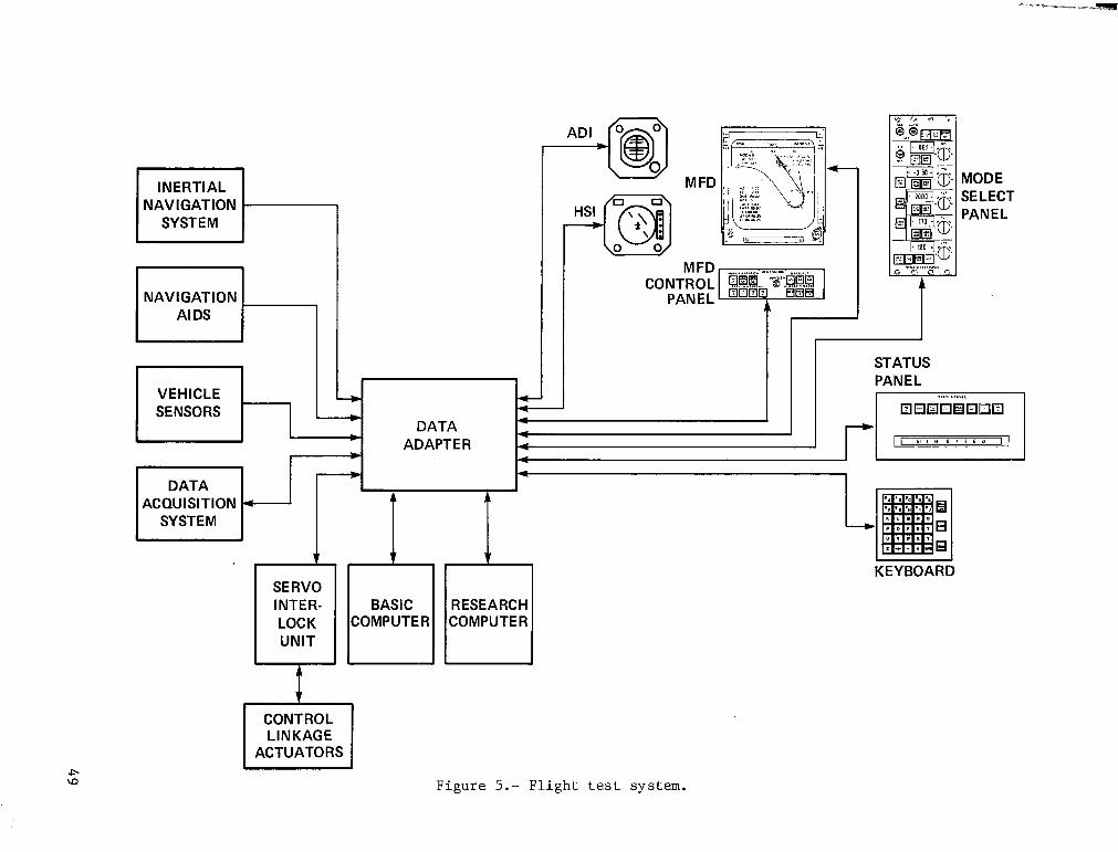
INERTIAL NAVIGATION

SYSTEM

F l - NAVIGATION

I VEHICLE I

M FD MODE SELECT PANEL

I " L

SENSORS DATA

ADAPTER

4 1

4 4

w - 4 r U I., I I., s I- E I: I,

4 DATA

SYSTEM

I

ACQUISITION 4 A t "$qk COMPUTER COMPUTER

CONTROL I LINKAGE I ACTUATORS

I

KEYBOARD -

Figure 5.- F l i g h t tes t system.

762 m AGL

GLIDE SLOPE

TRANSITION FROM -6.11" GLIDE SLOPE TO -2.5" GLIDE SLOPE

CENTERLINE

W I N DOWI (x = -1601 m)

WINDOW z (x = -914 m)

(WH

Figure 6.- Window l o c a t i o n s .

(WHERE YOU THINK YOU SHOULD BE)

GUIDANCE AND (WHERE YOU \ CONTROL ERROR THINK YOU ARE)

ERE YOU SHOULD BE

(WHERE YOU ARE)

ESTIMATED ORIGIN @"""

A I

t-@ '\ ACTUAL ORIGIN ACTUAL REFERENCE

Figure 7.- G r a p h i c a l d e f i n i t i o n of the guidance and control and s ta te e s t ima t ion e r r o r s i n t h e X-Y plane.

50

E

& a n a

Y

> K

-. 2 I 1 I I I I I I 1 I I I I I I

loo0 # E h a n a CT I

800

600

400

200

0 1 1

1.2

i - 1

- C L . .

0 -1.2 -1.4 -1.6 -1.8 I I

X-DISTANCE TO TOUCHDOWN, km

(a) Using INS-Kalman f i l t e r .

Figure 8.- Radar t rack of h e l i c o p t e r p o s i t i o n d u r i n g h e l i c a l a p p r o a c h e s .

51

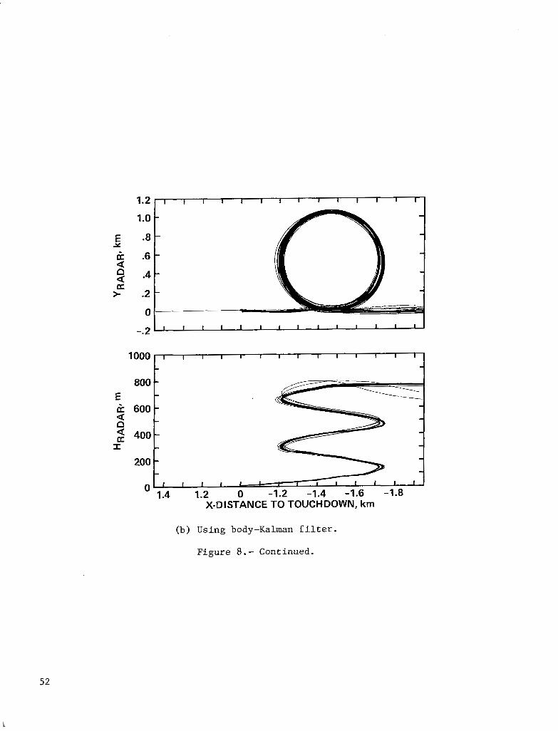
1.2

1 .o E -8

K .6 a Y

9 .4 CT > .2

0 I 1 I I I I 1 I I I I I I

loo0 ~

2 o o L - 0 1.4 A 1.2 0 -1.2 -1.4 -1.6 -1.8


(b) Using body-Kalman filter.

Figure 8. - Continued.

52

L

1.21 1 I I I I I I I I I I I I I

1.0

- E .8

-

- h .6 Y

a n a -4 -

U >. .2 -

0

-.2 L I I I I I I I I I I I I I

l o o o r ' I I I I I I I I I I I

800 E

200

0 1.4 1.2 0 -1.2 -1.4 -1.6 -1.8


(c'> Using body-complementary f i l t e r .

F igure 8.- Concluded.

53

E 100

a- 80

2 60 a w 40

-J -40 a -60 a

4 w I- -80

-100

(a) Lateral p o s i t i o n .

80 -HELIX 0

HELIX - K 60 -ENTRY 1/2 1-TURN 1-1/2 EXIT - K

UJ W 4 0 - J . 4 J. j. - 2

. . : .* .... ” 20 : ..:”-* ._.” . . .. *. -. e . - . . . . . . ............. .-...**A... ./ .. ........... m...y .> ... .7 . .

- . . . ...

-40 - -

. . . . . . .. .. a -

K -60 - W

-80 1 (b) a .” ~ ~ ~~ ~

8000 7000 6000 5000 4000 3000 2000 1000 0 DISTANCE TO TOUCHDOWN, m

(b) La tera l gu idance .

Figure 9.- Two-sigma e s t i m a t i o n e r r o r s f o r t h e INS-Kalman f i l t e r a p p r o a c h e s . ( 2 1 approaches)

54

t

80

-*O - (c) -

1 1 1 1 1 1 1 1 1 1 1 1 1 1 1

( c ) C r o s s - t r a c k s t a t e e s t i m a t i o n .

1 1 1 1 1 1 1 1 1 1 1 1 1 1 1 HELIX

ei= c3a - -

E -40- - - -

-80 - (d) -

1 1 1 1 1 1 1 1 1 1 1 1 1 1 1


(d) Along-track s t a t e e s t ima t ion .

F igure 9.- Concluded.

55

E u 0 ENTRY 1/2 1-TURN 1-1/2 EX1 T

5 40- z

-

0 - "-"-/_- -

1 1 1 1 1 1 1 1 1 1 1 1 1 1 1

80 - HELIX HELIX - U - + 4 J. s. + -

CAT I I I LS LIMIT ""_ " - -

v)

""""""

I r o - ... . . "

2 ="-" & \ - DH

2 -40 - -

- c - -

(a ) Vertical p o s i t i o n .

I

1 1 1 1 1 1 1 1 1 1 1 1 1 1 1


(b) Ver t ica l gu idance .

Figure 10.- Two-sigma ve r t i ca l pos i t i on , gu idance , and s t a t e e s t i m a t i o n e r r o r s f o r t h e INS-Kalman f i l t e r he l ica l approaches.

56

~~~ ~~

i " 1 1 1 1 1 1 1 1 1 1 1 1 1 1 1

80 HELIX HELIX - ENTRY 112

J. J- J. J- J- 1-TURN 1-112 EXIT

40 - -


(c ) Mean v e r t i c a l s t a t e e s t i m a t i o n e r r o r s .

Figure 10. - Concluded.

57

803 40

0

J -40 - 5 t- a -80 W >

80 0 3000 2000 1000 0 DISTANCE TO TOUCHDOWN, rn

Figure 11.- Composite v e r t i c a l g u i d a n c e e r r o r f o r t h e INS-Kalman f i l ter h e l i c a l approaches.

58

0 a a w z 0

1 a a

60

40

2% 0

-20 -40

-60

E 100- - , HELIX -

.. 3 -60

- - $ -80

- -

4 -100 (b) I


Figure 1 2 . - Two-sigma l a t e ra l p o s i t i o n , g u i d a n c e , a n d s t a t e e s t i m a t i o n e r r o r s f o r t h e body-Kalman f i l t e r h e l i c a l a p p r o a c h e s .

59

1 1 1 1 1 1 1 1 1 1 1 ,,t H ~ L I ~ HELIX’ 4 E ENTRY 1/2 1-TURN 1-1/2 EXIT

HELIX 1 1 1 1 1 1 1 1 1 1 1 1 1 1 1

HELIX - E_ 8o -ENTRY 112 1-TURN 1-1/2 EXIT

- (dl -

1 1 1 1 1 1 1 1 1 1 1 1 1 1 1


F i g u r e 1 2 . - Concluded.

60

IU 40 t s- J. z ,CAT II ILS LIMIT

"""" """"_ ~ - .. - ~~~

. .

er w -80 > ~~

E a 0

1 1-r- HELIX HELIX ENTRY 1/2 1-TURN 1 - 1 0 EXIT

) I L I I I ,

8000 7000 6000 5000 ' 4000 3000 2000 1000 0 1 1 1 1 1 1 1 1

DISTANCE TO TOUCHDOWN, m

Figure 13.- Two-sigma v e r t i c a l p o s i t i o n , g u i d a n c e , a n d s t a t e e s t i m a t i o n e r r o r s t h e body-Kalman f i l t e r h e l i c a l a p p r o a c h e s .

61

2 0

I 1 1 1 1 1 1 1 1 1 1 1 1 1 1 HELIX HELIX ~ -

L *O - ENTRY 1/2 1-TURN 1-1/2 EXIT

C 2 40 p J- J- J.

- 9 I- U

> "I- ( c ) -

1 1 1 1 1 1 1 1 1 1 1 1 1 1 l 8000 7000 6000 5000 4000 3000 2000 1000 0


Figure 13.- Concluded.

62

I I I I I I

HELIX -

w k -80 - I I CAT. II ILS LIMIT J -100

I'\

a (a) ,,, I 1 1 I I I

E 100 cr' 0 80 CT 6o

-

~~~~

I 1 I I I I 1

- CT

- - HELIX 1/2 1-TURN 1-1/2 HELIX -

-40 - E -60 - - + -80

- .. .. . . . . . . a

- .. w

-

4 -100 ___~ (b) - ~ L 1 I I I 1 I


Figure 14 . - Two-sigma l a t e r a l p o s i t i o n and guidance errors for the body-complementary f i l t e r h e l i c a l a p p r o a c h e s .

6 3

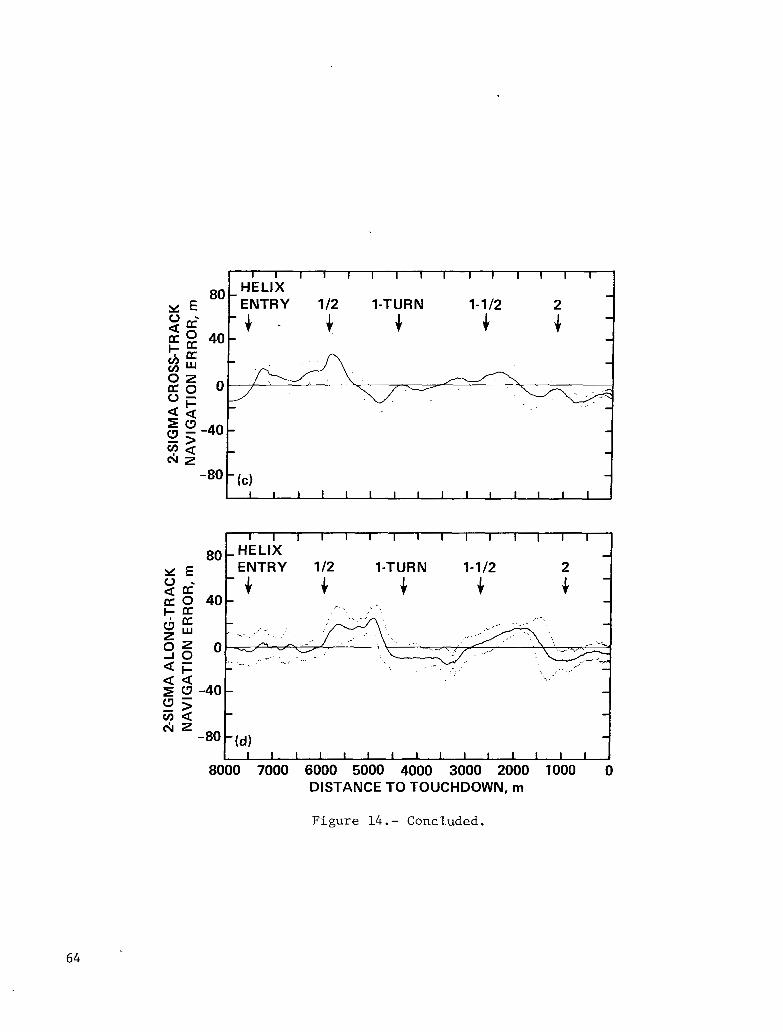
1 1 1 1 1 1 1 1 1 ~ 1 ~ ~ 1 ~

80 - HELIX - ENTRY 1/2 1-TURN 1-112 2

L - -80 -(dl -

1 1 1 1 1 1 1 1 1 1 1 1 1 1 1

8000 7000 6000 5000 4000 3000 2000 1000 0 DISTANCE TO TOUCHDOWN, rn

Figure 14.- Concluded.

64

HELIX

0 ENTRY a

z --"""" """," ""_"" """"_

2 """" ------- DH 2 -40

u L I I

1 1 1 l 1 1 1 1 1 1 1 1 1 1

E ) 1 1 1 1 1 1 1 1 1 1 1 1 1 1 1 )

a 40

$ -80t (b) > 1 1 1 1 1 1 1 1 1 1 1 I I I I


z 2 8 0 - - I-

I 6 40

- W E -

1 1 1 1 1 1 1 1 1 1 1 1 1 1 ~

a - - - -

K- 0 "".- $

~~ ~ "

m a - I w

-

u - - a -40

g! -80 - (c )

k K

- - -

1 1 1 1 1 1 1 1 1 1 1 1 1 1 1

8000 7000 6000 5000 4000 3000 2000 1000 0 DISTANCE TO TOUCHDOWN, rn

Figure 15.- Two-sigma ve r t i ca l pbs i t i on , gu idance , and state e s t i m a t i o n e r r o r s f o r t h e body-complementary f i l t e r h e l i c a l a p p r o a c h e s .

65

2 0

v) 0

0 -10 - $ 1

CAT II ILS WINDOW

I

0

I- K Lu a) > -20 I I I I I I

-30 -20 -10 0 10 20 30 LATERAL POSITION ERROR, m

0

I-

u a

-30 -20 -10 0 10 20 30 LATERAL GUIDANCE ERROR, m

E

0

0 a I-

I

0 a J

3 C) -20 I I I I I I

w a -30 -20 -10 0 10 20 30 > LATERAL STATE ESTlMATlnhI FnnOR. m

Figure 16.- Pos i t ion , gu idance , and s t a t e e s t i m a t i o n e r r o r d i s p e r s i o n s a t 30-m d e c i s i o n h e i g h t f o r INS-Kalman f i l t e r h e l i c a l a p p r o a c h e s .

66

I

5 a 20[ 10 CAT I1 ILS WINDOW

0 0

I- a -

(a)

$ -20 I I I I I 1

-30 -20 -10 0 10 20 30 LATERAL POSITION ERROR, m

:-lo: I- er 2 0 - -20 -30 -20 -10 0 10 20 30

LATERAL GUIDANCE ERROR, m

E

kz a c -10 4

9 E -20-30 -40 -;o

(C) I I I I

0 10 20 30 W > LATERAL STATE ESTIMATION ERROR, m

1 7 . - Posi t ion, guidance, and s ta te e s t i m a t i o n e r r o r d i s p e r s i o n s a t t h e 30-m dec i s ion he igh t f o r t h e body-Kalman f i l t e r h e l i c a l a p p r o a c h e s .

67

. . c

CT 0 0: 5 10 - CAT II ILS

0 0 WINDOW 0 - +

K

> -50 -40 -30 -20 -10 0 10 20 30 w -201 I I I I I I I I

LATERAL POSITION ERROR, m

I-

> -50 -40 -30 -20 -10 0 I 1 I I I I I _ I

W E -20 1 10 20 30 LATERAL GUIDANCE ERROR, m

E

a VI -10 F

0 0 o w +

-I

5 (C)

I I I I I I I I

LATERAL STATE ESTIMATION ERROR, m 0: -50 -40 -30 -20 -10 0 10 20 30 > F -20 W

Figure 18.- Posi t ion, guidance, and s ta te e s t i m a t i o n e r r o r d i s p e r s i o n s a t t h e 30-m d e c i s i o n h e i g h t f o r t h e body-complementary f i l t e r h e l i c a l a p p r o a c h e s .

68

K E 10- CAT II ILS z b 0 -

WINDOW 0

v)

-

2 J

2 . . a -10- 0 I- (a) K - w> -20-30 -10 -io 0 I I I

10 20 30 LATERAL POSITION ERROR, m

E 101 W 0 z a 0 n

2 - - lo- (b) !-

., -30 -20 -10 0 10 20 30 E -20 --I

I I I I I " ~

LATERAL GUIDANCE ERROR, m

E

0 K a W z 0 2o t c I in

w o W I I- a I L I

9 - E -20-30 -;o - i o

(C) I- I I I I

0 10 20 30 > LATERAL NAVIGATION ERROR, m

Figure 19.- Stra ight - in approach pos i t ion , gu idance , and s ta te e s t i m a t i o n e r r o r s a t 30-m d e c i s i o n h e i g h t f o r t h e body-Kalman f i l t e r .

69

E 40[ INS-KALMAN

K. 30 1 TOUCHDOWN PAD

W

2-SIGMA GUIDANCE ERROR

-30 -20 -1 0 0 10 20 30 LATERAL ERROR, m

BODY-COMPLEMENTARY BODY-KALMAN 40

E

0 30

20

-I 10 z a n - 0 2 + -10 c3

-20

W

- s

-30

2-SIGMA GUiDANCE ERROR

B

CD

I I I

-20 -10 0 10 20 30 -30-20 -10 0 10 20 30 LATERAL ERROR, m LATERAL ERROR, m

( a ) P o s i t i o n d i s p e r s i o n s .

Figure 20.- Helical approach a t hover.

70

E 101 I J

z a 0- n 3 -10- t w -20

-

- z

E, 30r INS-KALMAN

K Lu “1 10 T I LANDING PAD

3 -30’ -10 - i o 1b i o i o LATERAL ERROR, m

J I

BODY-KALMAN

2 -30 -20 -10 0 IO 20 30 -30 -20 -10 0 10 20 30 LATERAL ERROR, rn LATERAL ERROR, m

(b) Guidance dispers ions.

F igure 20.- Continued.

71

INS-KALMAN

I 1 I I I

-30 -20 -10 0 10 20 30 LATERAL ERROR, m

0

W I

J 10- a E 0 -

lz -10

z 3

c3 -

g -20 - -J

I I I I I I

LATERAL ERROR, m -30 -20 -10 0 10 20 30

t

BODY-KALMAN

I I I I I I

-30 -20 -10 0 10 20 30 LATERAL ERROR, m

(c ) S ta te e s t i m a t i o n d i s p e r s i o n s .

F igure 20. - Concluded.

72

50 -

E 4 0 - K 0 30- K K w 2 0 - 4 9 1 0 -

5 0 -

s -20 -

- k

-10 - z .

I I I

-30 -20 -10 0 10 20 30 L" t

LATERAL ERROR, m

Figure 21.- S t r a igh t - in app roach pos i t i on d i spe r s ions a t hover.

20- INS-KALMAN

0- m $ -20 I - I I 1 I I I I I I

y- 20-BODY-KALMAN W

z a 0- -20- I I I I I I 1 I 1 I

-I 2 20-BODY-COMPLEMENTARY

0 -20 1 I I I I I I I I I

0 30 60 90 120 150 180 210 240 270 300 TIME, sec

Figure 22.- R o l l ang le t i m e h i s t o r y i n t h e h e l i x .

73

100 I HELIX 2N D

E ENTRY TURN I . I

HELIX EXIT

I 2 40

UJ 20 K

I I - 0 3 E -20 N a -40 v)

- 4 -60 E

-80

-100 I 1 -~ - " 8000 7000 6000 5000 4000 3000 2000 1000 0


Figure 23.- MLS azimuth errors prototype system output .

E a-

a

E

2 w W

n

25 -

0

“ t -25 1 -50 I 1 1 1 1 1 1 1 1 1 1 1 1 ~ I


Figure 24.- MLS DME error.

75

cn h,

ID m l-t

a" r. =1 0

l-t (D

0 B

r "-"""" BASIC COMPUTER -IF RESEARCH COMPUTER 1 """"

I TO DISPLAY DISPLAY, AND SERVOS HARDWARE

GUIDANCE KALMAN -

AND CONTROL FILTER 4

I I

b I I I

I I

STATE COMPLEMEN- ESTlMA TARY FILTER I

A

I "+ ACCELERATION CALIBRATION 1

o(

I ACCELERATION - CALCULATION VOR/DME TACAN

A

I BAR0 ALT RADAR ALT

I L """""

"""" -I WANDER ANGLE

ACCELERATION ESTIMATED RAW INERTIAL (RUNWAY POSITION AND MEASUREMENTS REFERENCE) VELOCITY

Y * - INTEGRATE

SMOOTH I NG AND VELOCITY

N A V A I D POSITION AND

GUIDANCE AND CONTROL

IMU R E F . ACCELERATION UNIT COMPUTE . - - TRANSIT ION 'I F O R POSITION

t t 1 I I

STATE DATA REJECTION, CORRECTIONS STATE CORRECTION,

MEASUREMENT SELECTION A N D I N I T I A L I Z A T I O N

RAW NAVAID MEASUREMENTS

I ALGORITHMS I I I

Figure 26.- Block diagram of the s t a t e es t imat ion sys tems.

77

N AVA I D MEASUREMENTS

~

BAR0 ALTITUDE RADAR ALTITUDE M LS * FIRST-ORDER TACAN PREFILTERS AND VORIDME DATA-VALIDITY - REFERENCE -

* REFERENCE SELECTION AND

CALCULATION MLS ELEVATION * RAW ALTITUDE

* CHECKS SELECTION A A

X.Y - A

V MEASUREMENT RATE CALCULATION

RAW x,y CALCULATION

RAW x,y FOR LEVEL FILTERS ++

* A

X .V 1 - INERTIAL INSTRU- MENTATION AND

THIRD-ORDER

FILTERS SOFTWARE 4 NAVIGATION +

RAW ALTITUDE FOR VERTICAL FILTER

Figure 27.- Block diagram of complementary filters.

78

RAW MEASUREMENT .I

FILTERED MEASUREMENT TOLERANCE

TEST 4 - , LIMITER

S

I 4

MEASUREMENT TYPE TOLERANCE

TACAN BRG f 5 deg

TACAN RNG ? 457 rn (f1500 ft)

VOR BRG * 5 deg

VOR RNG f 457 rn (* 1500 ft)

MLS ELEV. ? 5 deg

MLS AZIMUTH ? 2 deg

MLS RNG f 457 rn (f 1500 ft)

L IMIT LEVEL

* 10 deg

* 122 rn (?r 400 f t )

r 10 des

f 122 rn (f 400 f t )

? 10 deg

f 10 deg

f 122 rn (f 400 ft)

ESTIMATED RATE

TIME CONSTANT 7.45 sec

7.45 sec 7.45 7.45 sec 7.45 sec

2 sec

2 sec

2 sec

Figure 28.- Block diagram and parameters of the prefilters.

79

..

I I

DR

n

&gk bo”0 NAVIGATION VALID

FILTER GAINS

0.735 0.0375

NOTES:

XR = ACCELERATION FROM IMU ..

X k NAVAID-DERIVED POSITION FROM PREFILTER

XA = A/C VELOCITY RELATIVE TO AIRMASS (X-COMPONENT)

X, = WIND VELOCITY (X-COMPONENT)

DR = DEAD-RECKONING MODE

I = INITIALIZATION

Figure 29.- Third-order s t a t e e s t i m a t i o n f i l t e r f o r x channel.

80

NOTES h = ALTITUDE COMPONENT.OF ACCELERATION FROM IMU .. 6 = ESTlMATED ALTITUDE RATE h = ESTIMATED ALTITUDE h, = RAW ALTITUDE FROM MEASUREMENT SELECTION LOGIC

GAINS Kq = 0.24 sec" K2 = 0.024 s ~ c - ~ K3 = 0.001 s ~ c - ~

Figure 30.- Third-order s t a t e e s t i m a t i o n f i l t e r f o r a l t i t u d e channel.

20 Hz 20 Hz

RAW IMU ~

EQUATIONS CALCULATIONS DATA AfiDVELOClTY NAVIGATION , REFERENCE, ACCELERATION

RUNWAY ESTIMATED POSITION - A 20 Hz

~ POSITION AND

+

COMPUTER 10 Hz

- VELOCITY SMOOTHING .. LOG IC TO BASIC

RAW NAVAID MEASUREMENT

-1 PREPROCESSING

MEASUREMENT 4 * REJECTION AND

1 - ESTIMATED STATE ERROR

MEASUREMENT

1 Hz LOGIC ALGORITHM * SELECTION FILTER

Figure 31.- Block diagram of t h e Kalman f i l t e r s ta te est imat ion system.

82

ORIGINAL TRUE AIRSPEED SENSOR LOCATION

NOSE BOOM STATIC PRESSU

TRUE AIRSPEED

Figure 32.- Ai rspeed sensor and s ta t ic -pressure loca t ions .

83

a

E

; 0;

L -10 z g -201 I I 1 1 I 1 I I J 0 15 30 45 60 75 90 105 120 Q TIM E, sec

(a) O r i g i n a l s e n s o r l o c a t i o n s .

F igure 33.- Time h i s t o r y of a level tu rn .

84

u W c E d W W n cn oc a W 3 a I-

E oc- 0 oc oc w

W a

42

38

34

30

28

tJ -10

a

E Fj -zoo 1 15 30 45 60 75 90 105 120

TIME, sec

(b) Shorn i n s t a l l e d .

F igu re 33 . - Concluded.

85

., :. -,

1. Report No. 3. Recipient's Catalog No. 2. Government Accession No. NASA TP-2109

4. Title and Subtitle 5. Report Date

HELICAL AUTOMATIC APPROACHES OF HELICOPTERS WITH MICROWAVE LANDING SYSTEMS 6. Performing Organization Code

December 1982

7. Author(sJ 8. Performing Organization Report No. John D. Foster, Leonard A. McGee, and Daniel C. Dugan A-9034

10. Work Unit No. 9. Performing Organization Name and Address 532-01-11

NASA Ames Research Center Moffett Field, Calif . 94035 I 1 1 . Contract or Grant No.

13. Type of Report and Period Covered 12. Sponsoring Agency Name and Address

14. Sponsoring Agency Code National Aeronautics and Space Administration

Technical Publication

Washington, D.C. 20546

15. Supplementary Notes Point of contact: John D. Foster, Ames Research Center, Moffett Field, CA 94035

M/S 237-11, (415)965-6577, FTS 448-6577

16. Abstract

A program i s under way a t Ames Research Center to develop a da ta .base for es tab l i sh ing navigation and guidance concepts for al l-weather operation of rotorcraft . One of the ob jec t ives is t o examine the feasibi l i ty of conduct ing s imultaneous rotorcraf t and conventional fixed-wing, non- interfer ing, landing operat ions in instrument meteorological condi t ions (IMC) at a i r p o r t s equipped with microwave landing systems (MISS) f o r fixed-wing t r a f f i c .

One way to accomplish this objective i s t o have r o t o r c r a f t f l y s p i r a l approach paths i n airspace separate from t h a t of the f ixed-wing traffic. Rotorcraft instrument-fl ight-rules (IFR) approaches could use the airspace along the edge of the M S lateral coverage, which would allow complete separation from fixed-wing traffic.

An i n i t i a l test program to invest igate the feasibi l i ty of conduct ing automatic hel ical approaches was completed, using the MLS a t Crows Landing near Ames. These tests were flown on board a UH-1H helicopter equipped with a digital automatic landing system. A t o t a l of 48 automatic approaches and landings were flown along a two-turn hel ical descent , tangent to the center l ine of the MLS-equipped runway to determine helical f l ight performance and to provide a da ta base for com- par i son wi th fu ture f l igh ts for which the he l i ca l approach path w i l l be located near the edge of the M S coverage. In addition, 13 straight-in approaches were conducted. The performance with varying levels of state-estimation system sophistication w a s evaluated as p a r t o f t h e f l i g h t tests. The resu l t s ind ica te tha t he l ica l approaches to MLS-equipped runways are feas ib l e fo r ro to rc ra f t : and that the best posit ion accuracy was obtained using the Kalman-filter state-estimation with iner t ia l navigat ion systems (INS) sensors.

7. Key Words (Suggested by Author(s1) Helicopter automatic landing Helical approach path Digital autoland Microwave Landing System

19. Security Classif. (of this report)

Unclassified

18. Distribution Statement Unclassified - Unlimited

Subject Category - 04 ~

' this page) 21. No. of Pages 22. Price'

Unclassified 89 1 A05

"For sale by the National Technical Information Service, Springfield, Virginia 22161

NASA-Langley, 1982 .".; - ,

1 .. .

Helical 'Automatic 'of Helicopte'rs With Microwave Landing · Helical 'Automatic 'of Helicopte'rs...

Documents

Transcript of Helical 'Automatic 'of Helicopte'rs With Microwave Landing · Helical 'Automatic 'of Helicopte'rs...