HEIZER MUNSON OPERATIONS...ISBN-13: 978-0-13-413042-2 ISBN-10: 0-13-413042-1 9 780134 130422 90000...
43
OPERATIONS MANAGEMENT Sustainability and Supply Chain Management TWELFTH EDITION JAY HEIZER | BARRY RENDER | CHUCK MUNSON
Transcript of HEIZER MUNSON OPERATIONS...ISBN-13: 978-0-13-413042-2 ISBN-10: 0-13-413042-1 9 780134 130422 90000...

ISBN-13: 978-0-13-413042-2ISBN-10: 0-13-413042-1
9 780134 130422
9 0 0 0 0
OPER ATIONS MANAGEMENTSustainability and Supply Chain Management
TWELFTH EDITION
OPER
AT
ION
S MA
NA
GE
ME
NT
Sustain
ability and
Supply C
hain
Man
agemen
t
TWELFTH EDITION
JAY HEIZER | BARRY RENDER | CHUCK MUNSON
HEIZERRENDERMUNSON
www.pearsonhighered.com
IMPROVING RESULTSA proven way to help individual students achieve
the goals that educators set for their course.
ENGAGING EXPERIENCESDynamic, engaging experiences that personalize and
activate learning for each student.
AN EXPERIENCED PARTNERFrom Pearson, a long-term partner with a true grasp
of the subject, excellent content, and an eye on the future of education.
Pearson’s MyLab™

487487
CHAPTER O U T L I N E
12
◆
The Importance of Inventory 490 ◆
Managing Inventory 491
◆
Inventory Models 495
◆
Inventory Models for Independent Demand 496
◆
Probabilistic Models and Safety Stock 508
◆
Single-Period Model 513
◆
Fixed-Period ( P ) Systems 514
GLOBAL COMPANY PROFILE: Amazon.com
CH
AP
TE
R
Inventory Management
1010OMOM STRATEGY DECISIONS
• • Design of Goods and Services
• • Managing Quality
• • Process Strategy
• • Location Strategies
• • Layout Strategies
• • Human Resources
• • Supply-Chain Management
• • Inventory Management
jj Independent Demand ( Ch. 12 ) jj Dependent Demand ( Ch. 14 )
jj Lean Operations ( Ch. 16 )
• • Scheduling
• • Maintenance
Ala
ska
Airl
ines
M16_HEIZ0422_12_SE_C12.indd 487M16_HEIZ0422_12_SE_C12.indd 487 05/11/15 5:03 PM05/11/15 5:03 PM

Inventory Management Provides Competitive Advantage at Amazon.com
GLOBAL COMPANY PROFILE Amazon.com
C H A P T E R 1 2
488
When Jeff Bezos opened his revolutionary business in 1995, Amazon.com was intended
to be a “virtual” retailer—no inventory, no warehouses, no overhead—just a bunch of
computers taking orders for books and authorizing others to fill them. Things clearly
didn’t work out that way. Now, Amazon stocks millions of items of inventory, amid hundreds of
thousands of bins on shelves in over 150 warehouses around the world. Additionally, Amazon’s
1. You order three items, and a computer in Seattle takes charge. A computer assigns your order—a book,
a game, and a digital camera—to one of Amazon’s
massive U.S. distribution centers.
2. The “flow meister” at the distribution center receives your order. She determines which workers go
where to fill your order.
Mar
ilyn
New
ton/
Ren
o G
azet
te-J
ourn
al
3. Amazon’s current system doubles the picking speed of manual operators and drops the error rate to nearly zero.
Ber
nhar
d C
lass
en/A
lam
y
Ben
Caw
thra
/Sip
a U
SA
/New
scom
4. Your items are put into crates on moving belts. Each
item goes into a large yellow crate that contains many
customers’ orders. When full, the crates ride a series of
conveyor belts that wind more than 10 miles through the
plant at a constant speed of 2.9 feet per second. The bar
code on each item is scanned 15 times, by machines and
by many of the 600 workers. The goal is to reduce errors to
zero—returns are very expensive.
M16_HEIZ0422_12_SE_C12.indd 488M16_HEIZ0422_12_SE_C12.indd 488 05/11/15 5:03 PM05/11/15 5:03 PM

489
REX
/New
scom
5. All three items converge in a chute and then inside a box. All the crates
arrive at a central point where bar codes
are matched with order numbers to
determine who gets what. Your three
items end up in a 3-foot-wide chute—
one of several thousand—and are placed
into a corrugated box with a new bar
code that identifies your order. Picking is
sequenced to reduce operator travel.
6. Any gifts you’ve chosen are wrapped by hand. Amazon trains an
elite group of gift wrappers, each of
whom processes 30 packages an hour.
7. The box is packed, taped, weighed, and labeled before leaving the warehouse in a truck. A typical plant is designed to ship as
many as 200,000 pieces a day. About 60% of
orders are shipped via the U.S. Postal Service;
nearly everything else goes through United
Parcel Service.
8. Your order arrives at your doorstep. In 1 or
2 days, your order is delivered. Adr
ian
She
rrat
t/A
lam
y
and management. The time to receive, process, and position
the stock in storage and to then accurately “pull” and pack-
age an order requires a labor investment of less than 3 min-
utes. And 70% of these orders are multiproduct orders. This
underlines the high benchmark that Amazon has achieved.
This is world-class performance.
When you place an order with Amazon
.com , you are doing business with
a company that obtains competitive
advantage through inventory management.
This Global Company Profile shows how
Amazon does it.
software is so good that
Amazon sells its order taking,
processing, and billing expertise
to others. It is estimated that
200 million items are now avail-
able via the Amazon Web site. Bezos expects the customer experience at Amazon to
be one that yields the lowest price, the fastest delivery, and
an error-free order fulfillment process so no other contact with
Amazon is necessary. Exchanges and returns are very expensive.
Managing this massive inventory precisely is the key for
Amazon to be the world-class leader in warehouse automation
M16_HEIZ0422_12_SE_C12.indd 489M16_HEIZ0422_12_SE_C12.indd 489 05/11/15 5:03 PM05/11/15 5:03 PM
490
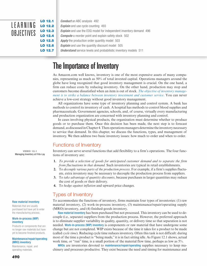
The Importance of Inventory As Amazon.com well knows, inventory is one of the most expensive assets of many compa-nies, representing as much as 50% of total invested capital. Operations managers around the globe have long recognized that good inventory management is crucial. On the one hand, a firm can reduce costs by reducing inventory. On the other hand, production may stop and customers become dissatisfied when an item is out of stock. The objective of inventory manage-ment is to strike a balance between inventory investment and customer service . You can never achieve a low-cost strategy without good inventory management.
All organizations have some type of inventory planning and control system. A bank has methods to control its inventory of cash. A hospital has methods to control blood supplies and pharmaceuticals. Government agencies, schools, and, of course, virtually every manufacturing and production organization are concerned with inventory planning and control.
In cases involving physical products, the organization must determine whether to produce goods or to purchase them. Once this decision has been made, the next step is to forecast demand, as discussed in Chapter 4 . Then operations managers determine the inventory necessary to service that demand. In this chapter, we discuss the functions, types, and management of inventory. We then address two basic inventory issues: how much to order and when to order.
Functions of Inventory Inventory can serve several functions that add flexibility to a firm’s operations. The four func-tions of inventory are:
1. To provide a selection of goods for anticipated customer demand and to separate the firm from fluctuations in that demand. Such inventories are typical in retail establishments.
2. To decouple various parts of the production process . For example, if a firm’s supplies fluctu-ate, extra inventory may be necessary to decouple the production process from suppliers.
3. To take advantage of quantity discounts , because purchases in larger quantities may reduce the cost of goods or their delivery.
4. To hedge against inflation and upward price changes.
Types of Inventory To accommodate the functions of inventory, firms maintain four types of inventories: (1) raw material inventory, (2) work-in-process inventory, (3) maintenance/repair/operating supply (MRO) inventory, and (4) finished-goods inventory.
Raw material inventory has been purchased but not processed. This inventory can be used to de-couple (i.e., separate) suppliers from the production process. However, the preferred approach is to eliminate supplier variability in quality, quantity, or delivery time so that separation is not needed. Work-in-process (WIP) inventory is components or raw material that have undergone some change but are not completed. WIP exists because of the time it takes for a product to be made (called cycle time ). Reducing cycle time reduces inventory. Often this task is not difficult: during most of the time a product is “being made,” it is in fact sitting idle. As Figure 12.1 shows, actual work time, or “run” time, is a small portion of the material flow time, perhaps as low as 5%.
MROs are inventories devoted to maintenance/repair/operating supplies necessary to keep ma-chinery and processes productive. They exist because the need and timing for maintenance and
L E A R N I N G OBJECTIVES
LO 12.1 Conduct an ABC analysis 492 LO 12.2 Explain and use cycle counting 493 LO 12.3 Explain and use the EOQ model for independent inventory demand 496 LO 12.4 Compute a reorder point and explain safety stock 502 LO 12.5 Apply the production order quantity model 503 LO 12.6 Explain and use the quantity discount model 505 LO 12.7 Understand service levels and probabilistic inventory models 511
VIDEO 12.1 Managing Inventory at Frito-Lay
Raw material inventory
Materials that are usually
purchased but have yet to enter
the manufacturing process.
Work-in-process (WIP) inventory
Products or components that are
no longer raw materials but have
yet to become finished products.
Maintenance/repair/operating (MRO) inventory
Maintenance, repair, and
operating materials.
M16_HEIZ0422_12_SE_C12.indd 490M16_HEIZ0422_12_SE_C12.indd 490 05/11/15 5:03 PM05/11/15 5:03 PM

CHAPTER 12 | INVENTORY MANAGEMENT 491
repair of some equipment are unknown. Although the demand for MRO inventory is often a function of maintenance schedules, other unscheduled MRO demands must be anticipated. Finished-goods inventory is completed product awaiting shipment. Finished goods may be inven-toried because future customer demands are unknown.
Managing Inventory Operations managers establish systems for managing inventory. In this section, we briefly examine two ingredients of such systems: (1) how inventory items can be classified (called ABC analysis ) and (2) how accurate inventory records can be maintained. We will then look at inventory control in the service sector.
ABC Analysis ABC analysis divides on-hand inventory into three classifications on the basis of annual dollar volume. ABC analysis is an inventory application of what is known as the Pareto principle(named after Vilfredo Pareto, a 19th-century Italian economist). The Pareto principle states that there are a “critical few and trivial many.” The idea is to establish inventory policies that focus resources on the few critical inventory parts and not the many trivial ones. It is not real-istic to monitor inexpensive items with the same intensity as very expensive items.
To determine annual dollar volume for ABC analysis, we measure the annual demand of each inventory item times the cost per unit . Class A items are those on which the annual dollar volume is high. Although such items may represent only about 15% of the total inventory items, they represent 70% to 80% of the total dollar usage. Class B items are those inventory items of medium annual dollar volume. These items may represent about 30% of inventory items and 15% to 25% of the total value. Those with low annual dollar volume are Class C , which may represent only 5% of the annual dollar volume but about 55% of the total inventory items.
Graphically, the inventory of many organizations would appear as presented in Figure 12.2 .
95% 5%
Input Wait forinspection
Wait tobe moved
Movetime
Wait in queuefor operator
Setuptime
Runtime
Output
Cycle time
Figure 12.1
The Material Flow Cycle
Most of the time that work is in-process (95% of the cycle time) is not productive time.
Finished-goods inventory
An end item ready to be sold, but
still an asset on the company’s
books.
ABC analysis
A method for dividing on-hand
inventory into three classifications
based on annual dollar volume.
STUDENT TIP A, B, and C categories need
not be exact. The idea is to
recognize that levels of control
should match the risk.
A items80706050403020100
Per
cent
age
of a
nnua
l dol
lar
usag
e
10 20 30 40 50 60 70 80 90 100
B itemsC items
Percentage of inventory items
Figure 12.2
Graphic Representation of ABC
Analysis
M16_HEIZ0422_12_SE_C12.indd 491M16_HEIZ0422_12_SE_C12.indd 491 05/11/15 5:03 PM05/11/15 5:03 PM
492 PART 3 | MANAGING OPERATIONS
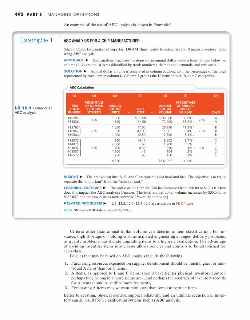
Criteria other than annual dollar volume can determine item classification. For in-stance, high shortage or holding cost, anticipated engineering changes, delivery problems, or quality problems may dictate upgrading items to a higher classification. The advantage of dividing inventory items into classes allows policies and controls to be established for each class.
Policies that may be based on ABC analysis include the following:
1. Purchasing resources expended on supplier development should be much higher for indi-vidual A items than for C items.
2. A items, as opposed to B and C items, should have tighter physical inventory control; perhaps they belong in a more secure area, and perhaps the accuracy of inventory records for A items should be verified more frequently.
3. Forecasting A items may warrant more care than forecasting other items.
Better forecasting, physical control, supplier reliability, and an ultimate reduction in inven-tory can all result from classification systems such as ABC analysis.
Example 1 ABC ANALYSIS FOR A CHIP MANUFACTURER
Silicon Chips, Inc., maker of superfast DRAM chips, wants to categorize its 10 major inventory items using ABC analysis.
APPROACH c ABC analysis organizes the items on an annual dollar-volume basis. Shown below (in columns 1–4) are the 10 items (identified by stock numbers), their annual demands, and unit costs.
SOLUTION c Annual dollar volume is computed in column 5, along with the percentage of the total represented by each item in column 6. Column 7 groups the 10 items into A, B, and C categories.
ABC Calculation
(1) (2) (3) (4) (5) (6) (7)
ITEM STOCK
NUMBER
PERCENTAGE OF NUMBER
OF ITEMS STOCKED
ANNUAL VOLUME (UNITS) 3
UNIT COST 5
ANNUAL DOLLAR VOLUME
PERCENTAGE OF ANNUAL
DOLLAR VOLUME CLASS
#10286 #11526 20% 1,000
500 $ 90.00 154.00
$ 90,000 77,000
38.8% 33.2% 72% A
A
#12760 #10867 #10500
30% 1,550
350 1,000
17.00 42.86 12.50
26,350 15,001 12,500
11.3% 6.4% 5.4%
23% B B B
#12572 #14075 #01036 #01307 #10572
50%
600 2,000
100 1,200
250
14.17 .60
8.50 .42 .60
8,502 1,200
850 504 150
3.7% .5% .4% .2% .1%
5%
C C C C C
8,550 $232,057 100.0%
LO 12.1 Conduct an
ABC analysis
INSIGHT c The breakdown into A, B, and C categories is not hard and fast. The objective is to try to separate the “important” from the “unimportant.”
LEARNING EXERCISE c The unit cost for Item #10286 has increased from $90.00 to $120.00. How does this impact the ABC analysis? [Answer: The total annual dollar volume increases by $30,000, to $262,057, and the two A items now comprise 75% of that amount.]
RELATED PROBLEMS c 12.1, 12.2, 12.3 (12.5–12.6 are available in MyOMLab)
EXCEL OM Data File Ch12Ex1.xls can be found in MyOMLab.
J
6
(')
'*
J
6
(')
'*
An example of the use of ABC analysis is shown in Example 1 .
M16_HEIZ0422_12_SE_C12.indd 492M16_HEIZ0422_12_SE_C12.indd 492 05/11/15 5:03 PM05/11/15 5:03 PM

CHAPTER 12 | INVENTORY MANAGEMENT 493
Record Accuracy Record accuracy is a prerequisite to inventory management, production scheduling, and, ulti-mately, sales. Accuracy can be maintained by either periodic or perpetual systems. Periodic systems require regular (periodic) checks of inventory to determine quantity on hand. Some small retailers and facilities with vendor-managed inventory (the vendor checks quantity on hand and resupplies as necessary) use these systems. However, the downside is lack of control between reviews and the necessity of carrying extra inventory to protect against shortages.
A variation of the periodic system is a two-bin system. In practice, a store manager sets up two containers (each with adequate inventory to cover demand during the time required to receive another order) and places an order when the first container is empty.
Alternatively, perpetual inventory tracks both receipts and subtractions from inventory on a continuing basis. Receipts are usually noted in the receiving department in some semiauto-mated way, such as via a bar-code reader, and disbursements are noted as items leave the stock-room or, in retailing establishments, at the point-of-sale (POS) cash register.
Regardless of the inventory system, record accuracy requires good incoming and out-going record keeping as well as good security. Stockrooms will have limited access, good housekeeping, and storage areas that hold fixed amounts of inventory. In both manufactur-ing and retail facilities, bins, shelf space, and individual items must be stored and labeled accurately. Meaningful decisions about ordering, scheduling, and shipping, are made only when the firm knows what it has on hand. (See the OM in Action box, “Inventory Accuracy at Milton Bradley.”)
Cycle Counting Even though an organization may have made substantial efforts to record inventory accurately, these records must be verified through a continuing audit. Such audits are known as cycle counting . Historically, many firms performed annual physical inventories. This practice often meant shut-ting down the facility and having inexperienced people count parts and material. Inventory records should instead be verified via cycle counting. Cycle counting uses inventory classifications developed through ABC analysis. With cycle counting procedures, items are counted, records are verified, and inaccuracies are periodically documented. The cause of inaccuracies is then traced and appropriate remedial action taken to ensure integrity of the inventory system. A items will be counted frequently, perhaps once a month; B items will be counted less frequently, perhaps once a quarter; and C items will be counted perhaps once every 6 months. Example 2 illustrates how to compute the number of items of each classification to be counted each day.
Cycle counting
A continuing reconciliation of
inventory with inventory records.
OM in Action Inventory Accuracy at Milton Bradley
Milton Bradley, a division of Hasbro, Inc., has been manufacturing toys for
150 years. Founded by Milton Bradley in 1860, the company started by making
a lithograph of Abraham Lincoln. Using his printing skills, Bradley developed
games, including The Game of Life, Chutes and Ladders, Candy Land, Scrab-
ble, and Lite Brite. Today, the company produces hundreds of games, requiring
billions of plastic parts.
Once Milton Bradley has determined the optimal quantities for each
production run, it must make them and assemble them as a part of the proper
game. Some games require literally hundreds of plastic parts, including spin-
ners, hotels, people, animals, cars, and so on. According to Gary Brennan,
director of manufacturing, getting the right number of pieces to the right toys
and production lines is the most important issue for the credibility of the com-
pany. Some orders can require 20,000 or more perfectly assembled games
delivered to their warehouses in a matter of days.
Games with the incorrect number of parts and pieces can result in some very
unhappy customers. It is also time-consuming and expensive for Milton Bradley to
supply the extra parts or to have
toys or games returned. When
shortages are found during
the assembly stage, the entire
production run is stopped until
the problem is corrected.
Counting parts by hand
or machine is not always
accurate. As a result, Milton Bradley now weighs pieces and completed games
to determine if the correct number of parts have been included. If the weight
is not exact, there is a problem that is resolved before shipment. Using highly
accurate digital scales, Milton Bradley is now able to get the right parts in the
right game at the right time. Without this simple innovation, the company’s
most sophisticated production schedule would be meaningless.
Sources: Forbes (February 7, 2011); and The Wall Street Journal (April 15, 1999).
Ant
hony
Lab
be/ P
hoto
fulc
rum
.com
In this hospital, these vertically
rotating storage carousels provide
rapid access to hundreds of
critical items and at the same time
save floor space. This Omnicell
inventory management carousel
is also secure and has the added
advantage of printing bar code
labels.
Om
nice
ll
LO 12.2 Explain and
use cycle counting
M16_HEIZ0422_12_SE_C12.indd 493M16_HEIZ0422_12_SE_C12.indd 493 05/11/15 5:03 PM05/11/15 5:03 PM
494 PART 3 | MANAGING OPERATIONS
In Example 2 , the particular items to be cycle counted can be sequentially or randomly selected each day. Another option is to cycle count items when they are reordered.
Cycle counting also has the following advantages:
1. Eliminates the shutdown and interruption of production necessary for annual physical inventories.
2. Eliminates annual inventory adjustments. 3. Trained personnel audit the accuracy of inventory. 4. Allows the cause of the errors to be identified and remedial action to be taken. 5. Maintains accurate inventory records.
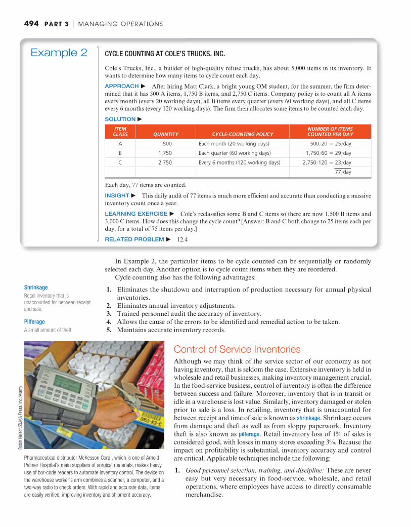
Example 2 CYCLE COUNTING AT COLE’S TRUCKS, INC.
Cole’s Trucks, Inc., a builder of high-quality refuse trucks, has about 5,000 items in its inventory. It wants to determine how many items to cycle count each day.
APPROACH c After hiring Matt Clark, a bright young OM student, for the summer, the firm deter-mined that it has 500 A items, 1,750 B items, and 2,750 C items. Company policy is to count all A items every month (every 20 working days), all B items every quarter (every 60 working days), and all C items every 6 months (every 120 working days). The firm then allocates some items to be counted each day.
SOLUTION c ITEM
CLASS QUANTITY CYCLE-COUNTING POLICY NUMBER OF ITEMS COUNTED PER DAY
A 500 Each month (20 working days) 500Y20 5 25Yday
B 1,750 Each quarter (60 working days) 1,750Y60 5 29Yday
C 2,750 Every 6 months (120 working days) 2,750Y120 5 23Yday
77Yday
Each day, 77 items are counted.
INSIGHT c This daily audit of 77 items is much more efficient and accurate than conducting a massive inventory count once a year.
LEARNING EXERCISE c Cole’s reclassifies some B and C items so there are now 1,500 B items and 3,000 C items. How does this change the cycle count? [Answer: B and C both change to 25 items each per day, for a total of 75 items per day.]
RELATED PROBLEM c 12.4
Shrinkage
Retail inventory that is
unaccounted for between receipt
and sale.
Pilferage
A small amount of theft.
Pharmaceutical distributor McKesson Corp., which is one of Arnold
Palmer Hospital’s main suppliers of surgical materials, makes heavy
use of bar-code readers to automate inventory control. The device on
the warehouse worker’s arm combines a scanner, a computer, and a
two-way radio to check orders. With rapid and accurate data, items
are easily verified, improving inventory and shipment accuracy.
Rob
in N
elso
n/ZU
MA
Pre
ss, In
c./A
lam
y
Control of Service Inventories Although we may think of the service sector of our economy as not having inventory, that is seldom the case. Extensive inventory is held in wholesale and retail businesses, making inventory management crucial. In the food-service business, control of inventory is often the difference between success and failure. Moreover, inventory that is in transit or idle in a warehouse is lost value. Similarly, inventory damaged or stolen prior to sale is a loss. In retailing, inventory that is unaccounted for between receipt and time of sale is known as shrinkage . Shrinkage occurs from damage and theft as well as from sloppy paperwork. Inventory theft is also known as pilferage . Retail inventory loss of 1% of sales is considered good, with losses in many stores exceeding 3%. Because the impact on profitability is substantial, inventory accuracy and control are critical. Applicable techniques include the following:
1. Good personnel selection, training, and discipline: These are never easy but very necessary in food-service, wholesale, and retail operations, where employees have access to directly consumable merchandise.
M16_HEIZ0422_12_SE_C12.indd 494M16_HEIZ0422_12_SE_C12.indd 494 05/11/15 5:03 PM05/11/15 5:03 PM

CHAPTER 12 | INVENTORY MANAGEMENT 495
2. Tight control of incoming shipments: This task is being addressed by many firms through the use of Universal Product Code (or bar code) and radio frequency ID (RFID) systems that read every incoming shipment and automatically check tallies against purchase orders. When properly designed, these systems—where each stock keeping unit (SKU; pronounced “skew”) has its own identifier—can be very hard to defeat.
3. Effective control of all goods leaving the facility: This job is accomplished with bar codes, RFID tags, or magnetic strips on merchandise, and via direct observation. Direct observation can be personnel stationed at exits (as at Costco and Sam’s Club wholesale stores) and in potentially high-loss areas or can take the form of one-way mirrors and video surveillance.
Successful retail operations require very good store-level control with accurate inventory in its proper location. Major retailers lose 10% to 25% of overall profits due to poor or inaccurate inventory records. 1 (See the OM in Action box, “Retail’s Last 10 Yards.”)
Inventory Models We now examine a variety of inventory models and the costs associated with them.
Independent vs. Dependent Demand Inventory control models assume that demand for an item is either independent of or depend-ent on the demand for other items. For example, the demand for refrigerators is independent of the demand for toaster ovens. However, the demand for toaster oven components is dependenton the requirements of toaster ovens.
This chapter focuses on managing inventory where demand is independent . Chapter 14 presents dependent demand management.
Holding, Ordering, and Setup Costs Holding costs are the costs associated with holding or “carrying” inventory over time. Therefore, holding costs also include obsolescence and costs related to storage, such as insurance, extra staffing, and interest payments. Table 12.1 shows the kinds of costs that need to be evalu-ated to determine holding costs. Many firms fail to include all the inventory holding costs. Consequently, inventory holding costs are often understated.
Ordering cost includes costs of supplies, forms, order processing, purchasing, clerical support, and so forth. When orders are being manufactured, ordering costs also exist, but they are a part
A handheld reader can scanRFID tags, aiding control of bothincoming and outgoing shipments.
OM in Action Retail’s Last 10 Yards
Retail managers commit huge resources to inventory and its management.
Even with retail inventory representing 36% of total assets, nearly 1 of 6 items
a retail store thinks it has available to its customers is not! Amazingly, close to
two-thirds of inventory records are wrong. Failure to have product available is
due to poor ordering, poor stocking, mislabeling, merchandise exchange er-
rors, and merchandise being in the wrong location. Despite major investments
in bar coding, RFID, and IT, the last 10 yards of retail inventory management is
a disaster.
The huge number and variety of stock keeping units (SKUs) at the retail
level adds complexity to inventory management. Does the customer really
need 32 different offerings of Crest toothpaste or 26 offerings of Colgate?
The proliferation of SKUs increases confusion, store size, purchasing,
inventory, and stocking costs, as well as subsequent markdown costs. With
so many SKUs, stores have little space to stock and display a full case of many
products, leading to labeling and “broken case” issues in the back room.
Supervalu, the nation’s 4th largest food retailer, is reducing the number of
SKUs by 25% as one way to cut costs and add focus to its own store-branded
items.
Reducing the variation in delivery lead time, improving forecasting ac-
curacy, and cutting the huge variety of SKUs may all help. But reducing the
number of SKUs may not improve customer service. Training and educating
employees about the importance of inventory management may be a better
way to improve the last 10 yards.
Sources: The Wall Street Journal (January 13, 2010); Management Science
(February 2005); and California Management Review (Spring 2001).
VIDEO 12.2 Inventory Control at Wheeled Coach
Ambulance
Holding cost
The cost to keep or carry inventory
in stock.
Ordering cost
The cost of the ordering process.
M16_HEIZ0422_12_SE_C12.indd 495M16_HEIZ0422_12_SE_C12.indd 495 05/11/15 5:03 PM05/11/15 5:03 PM

496 PART 3 | MANAGING OPERATIONS
of what is called setup costs. Setup cost is the cost to prepare a machine or process for manufac-turing an order. This includes time and labor to clean and change tools or holders. Operations managers can lower ordering costs by reducing setup costs and by using such efficient proce-dures as electronic ordering and payment.
In manufacturing environments, setup cost is highly correlated with setup time . Setups usually require a substantial amount of work even before a setup is actually performed at the work center. With proper planning, much of the preparation required by a setup can be done prior to shutting down the machine or process. Setup times can thus be reduced substantially. Machines and processes that traditionally have taken hours to set up are now being set up in less than a minute by the more imaginative world-class manufacturers. Reducing setup times is an excellent way to reduce inventory investment and to improve productivity.
Inventory Models for Independent Demand In this section, we introduce three inventory models that address two important questions: when to order and how much to order . These independent demand models are:
1. Basic economic order quantity (EOQ) model 2. Production order quantity model 3. Quantity discount model
The Basic Economic Order Quantity (EOQ) Model The economic order quantity (EOQ) model is one of the most commonly used inventory-control tech-niques. This technique is relatively easy to use but is based on several assumptions:
1. Demand for an item is known, reasonably constant, and independent of decisions for other items.
2. Lead time—that is, the time between placement and receipt of the order—is known and consistent.
3. Receipt of inventory is instantaneous and complete. In other words, the inventory from an order arrives in one batch at one time.
4. Quantity discounts are not possible. 5. The only variable costs are the cost of setting up or placing an order (setup or ordering
cost) and the cost of holding or storing inventory over time (holding or carrying cost). These costs were discussed in the previous section.
6. Stockouts (shortages) can be completely avoided if orders are placed at the right time.
With these assumptions, the graph of inventory usage over time has a sawtooth shape, as in Figure 12.3 . In Figure 12.3 , Q represents the amount that is ordered. If this amount is 500 dresses, all 500 dresses arrive at one time (when an order is received). Thus, the inventory
TABLE 12.1 Determining Inventory Holding Costs
CATEGORY
COST (AND RANGE) AS A PERCENTAGE OF INVENTORY VALUE
Housing costs (building rent or depreciation, operating cost, taxes, insurance) 6% (3–10%)
Material-handling costs (equipment lease or depreciation, power, operating cost) 3% (1–3.5%)
Labor cost (receiving, warehousing, security) 3% (3–5%)
Investment costs (borrowing costs, taxes, and insurance on inventory) 11% (6–24%)
Pilferage, scrap, and obsolescence (much higher in industries undergoing rapid change like tablets and smart phones)
3% (2–5%)
Overall carrying cost 26%
Note: All numbers are approximate, as they vary substantially depending on the nature of the business, location, and current interest rates.
Setup cost
The cost to prepare a machine or
process for production.
STUDENT TIP An overall inventory carrying cost of
less than 15% is very unlikely, but
this cost can exceed 40%, especially
in high-tech and fashion industries.
Setup time
The time required to prepare a
machine or process for production.
Economic order quantity (EOQ) model
An inventory-control technique
that minimizes the total of ordering
and holding costs.
LO 12.3 Explain and
use the EOQ model for
independent inventory
demand
M16_HEIZ0422_12_SE_C12.indd 496M16_HEIZ0422_12_SE_C12.indd 496 05/11/15 5:03 PM05/11/15 5:03 PM

CHAPTER 12 | INVENTORY MANAGEMENT 497
level jumps from 0 to 500 dresses. In general, an inventory level increases from 0 to Q units when an order arrives.
Because demand is constant over time, inventory drops at a uniform rate over time. (Refer to the sloped lines in Figure 12.3 .) Each time the inventory is received, the inventory level again jumps to Q units (represented by the vertical lines). This process continues indefinitely over time.
Minimizing Costs The objective of most inventory models is to minimize total costs. With the assumptions just given, significant costs are setup (or ordering) cost and holding (or carrying) cost. All other costs, such as the cost of the inventory itself, are constant. Thus, if we minimize the sum of setup and holding costs, we will also be minimizing total costs. To help you visualize this, in Figure 12.4 we graph total costs as a function of the order quantity, Q . The optimal order size, Q *, will be the quantity that minimizes the total costs. As the quantity ordered increases, the total number of orders placed per year will decrease. Thus, as the quantity ordered increases, the annual setup or ordering cost will decrease [ Figure 12.4 (a)]. But as the order quantity increases, the holding cost will increase due to the larger average inventories that are main-tained [ Figure 12.4 (b)].
As we can see in Figure 12.4 (c), a reduction in either holding or setup cost will reduce the total cost curve. A reduction in the setup cost curve also reduces the optimal order quantity (lot size). In addition, smaller lot sizes have a positive impact on quality and production flexibility. At Toshiba, the $77 billion Japanese conglomerate, workers can make as few as 10 laptop com-puters before changing models. This lot-size flexibility has allowed Toshiba to move toward a “build-to-order” mass customization system, an important ability in an industry that has product life cycles measured in months, not years.
You should note that in Figure 12.4 (c), the optimal order quantity occurs at the point where the ordering-cost curve and the carrying-cost curve intersect. This was not by chance. With the EOQ model, the optimal order quantity will occur at a point where the total setup cost is equal
STUDENT TIP If the maximum we can ever
have is Q (say, 500 units) and
the minimum is zero, then if
inventory is used (or sold) at a
fairly steady rate, the average
5 ( Q 1 0)Y2 5 Q Y2.
Inve
ntor
y le
vel
Order quantity = Q(maximum inventory
level)
Minimuminventory 0
Time
Average inventoryon hand
Q—2( )
Usage rateTotal order received Figure 12.3
Inventory Usage over Time
Setup (order) cost
Order quantity(a) Annual setup (order) cost (b) Annual holding cost
Ann
ual c
ost
(c) Total costs
Order quantity
Ann
ual c
ost
Holding costHolding cost
Setup (order) cost
Total cost for holdingand setup (order)
Order quantityOptimal orderquantity (Q*)
Minimumtotal cost
Ann
ual c
ost
Figure 12.4
Costs as a Function of Order Quantity
STUDENT TIP Figure 12.4 is the heart of EOQ
inventory modeling. We want to find
the smallest total cost (top curve),
which is the sum of the two curves
below it.
M16_HEIZ0422_12_SE_C12.indd 497M16_HEIZ0422_12_SE_C12.indd 497 05/11/15 5:03 PM05/11/15 5:03 PM

498 PART 3 | MANAGING OPERATIONS
to the total holding cost. 2 We use this fact to develop equations that solve directly for Q *. The necessary steps are:
1. Develop an expression for setup or ordering cost. 2. Develop an expression for holding cost. 3. Set setup (order) cost equal to holding cost. 4. Solve the equation for the optimal order quantity.
Using the following variables, we can determine setup and holding costs and solve for Q *:
Q 5 Number of units per order Q * 5 Optimum number of units per order (EOQ)
D 5 Annual demand in units for the inventory item S 5 Setup or ordering cost for each order H 5 Holding or carrying cost per unit per year
1. Annual setup cost 5 (Number of orders placed per year) 3 (Setup or order cost per order)
= ¢ Annual demandNumber of units in each order
≤ (Setup or order cost per order)
= ¢DQ≤ (S) =
DQ
S
2. Annual holding cost 5 (Average inventory level) 3 (Holding cost per unit per year)
= ¢Order quantity2
≤ (Holding cost per unit per year)
= ¢Q2≤(H) =
Q2
H
3. Optimal order quantity is found when annual setup (order) cost equals annual holding cost, namely:
DQ
S =Q2
H
4. To solve for Q *, simply cross-multiply terms and isolate Q on the left of the equal sign:
2DS = Q2H
Q2 =2DSH
Q * =A
2DSH
(12-1)
Now that we have derived the equation for the optimal order quantity, Q *, it is possible to solve inventory problems directly, as in Example 3 .
Example 3 FINDING THE OPTIMAL ORDER SIZE AT SHARP, INC.
Sharp, Inc., a company that markets painless hypodermic needles to hospitals, would like to reduce its inventory cost by determining the optimal number of hypodermic needles to obtain per order.
APPROACH c The annual demand is 1,000 units; the setup or ordering cost is $10 per order; and the holding cost per unit per year is $.50.
M16_HEIZ0422_12_SE_C12.indd 498M16_HEIZ0422_12_SE_C12.indd 498 05/11/15 5:03 PM05/11/15 5:03 PM
CHAPTER 12 | INVENTORY MANAGEMENT 499
SOLUTION c Using these figures, we can calculate the optimal number of units per order:
Q* =A
2DSH
Q* = A2(1,000)(10)
0.50= 240,000 = 200 units
INSIGHT c Sharp, Inc., now knows how many needles to order per order. The firm also has a basis for determining ordering and holding costs for this item, as well as the number of orders to be processed by the receiving and inventory departments.
LEARNING EXERCISE c If D increases to 1,200 units, what is the new Q *? [Answer: Q * 5 219 units.]
RELATED PROBLEMS c 12.7, 12.8, 12.9, 12.10, 12.11, 12.14, 12.15, 12.17, 12.29 (12.31, 12.32, 12.33a, 12.35a are available in MyOMLab)
EXCEL OM Data File Ch12Ex3.xls can be found in MyOMLab.
ACTIVE MODEL 12.1 This example is further illustrated in Active Model 12.1 in MyOMLab.
We can also determine the expected number of orders placed during the year ( N ) and the expected time between orders ( T ), as follows:
Expected number of orders = N =Demand
Order quantity=
DQ*
(12-2)
Expected time between orders = T =Number of working days per year
N (12-3)
Example 4 illustrates this concept.
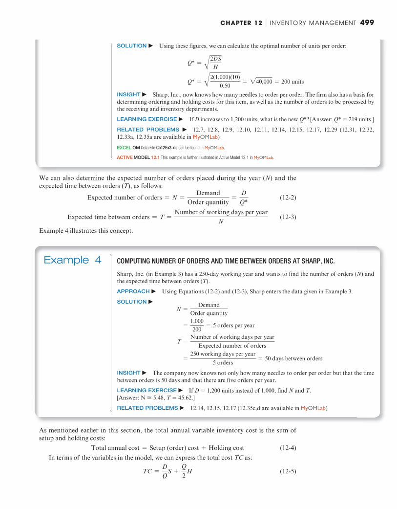
Example 4 COMPUTING NUMBER OF ORDERS AND TIME BETWEEN ORDERS AT SHARP, INC.
Sharp, Inc. (in Example 3 ) has a 250-day working year and wants to find the number of orders ( N ) and the expected time between orders ( T ).
APPROACH c Using Equations (12-2) and (12-3), Sharp enters the data given in Example 3 .
SOLUTION c N =
DemandOrder quantity
=1,000200
= 5 orders per year
T =Number of working days per year
Expected number of orders
=250 working days per year
5 orders= 50 days between orders
INSIGHT c The company now knows not only how many needles to order per order but that the time between orders is 50 days and that there are five orders per year.
LEARNING EXERCISE c If D 5 1,200 units instead of 1,000, find N and T . [Answer: N > 5.48, T 5 45.62.]
RELATED PROBLEMS c 12.14, 12.15, 12.17 (12.35c,d are available in MyOMLab)
As mentioned earlier in this section, the total annual variable inventory cost is the sum of setup and holding costs: Total annual cost = Setup (order) cost + Holding cost (12-4)
In terms of the variables in the model, we can express the total cost TC as:
TC =DQ
S +Q2
H (12-5)
M16_HEIZ0422_12_SE_C12.indd 499M16_HEIZ0422_12_SE_C12.indd 499 05/11/15 5:03 PM05/11/15 5:03 PM

500 PART 3 | MANAGING OPERATIONS
Inventory costs may also be expressed to include the actual cost of the material purchased. If we assume that the annual demand and the price per hypodermic needle are known values (e.g., 1,000 hypodermics per year at P 5 $10) and total annual cost should include purchase cost, then Equation (12-5) becomes:
TC =DQ
S +Q2
H + PD
Because material cost does not depend on the particular order policy, we still incur an annual material cost of D * P = (1,000)(+10) = +10,000. (Later in this chapter we will discuss the case in which this may not be true—namely, when a quantity discount is available.) 3
Robust Model A benefit of the EOQ model is that it is robust. By robust we mean that it gives satisfactory answers even with substantial variation in its parameters. As we have observed, determining accurate ordering costs and holding costs for inventory is often difficult. Consequently, a robust model is advantageous. The total cost of the EOQ changes little in the neighborhood of the minimum. The curve is very shallow. This means that variations in setup costs, holding costs, demand, or even EOQ make relatively modest differences in total cost. Example 6 shows the robustness of EOQ.
Example 5 COMPUTING COMBINED COST OF ORDERING AND HOLDING
Sharp, Inc. (from Examples 3 and 4 ) wants to determine the combined annual ordering and holding costs.
APPROACH c Apply Equation (12-5), using the data in Example 3 .
SOLUTION c TC =
DQ
S +Q2
H
=1,000200
(+10) +2002
(+.50)
= (5) (+10) + (100) (+.50) = +50 + +50 = +100
INSIGHT c These are the annual setup and holding costs. The $100 total does not include the actual cost of goods. Notice that in the EOQ model, holding costs always equal setup (order) costs.
LEARNING EXERCISE c Find the total annual cost if D 5 1,200 units in Example 3 . [Answer: $109.54.]
RELATED PROBLEMS c 12.11, 12.14, 12.15, 12.16 (12.33b,c; 12.35e; 12.36a,b are available in MyOMLab)
Robust
Giving satisfactory answers even
with substantial variation in the
parameters.
Example 6 EOQ IS A ROBUST MODEL
Management in the Sharp, Inc., examples underestimates total annual demand by 50% (say demand is actually 1,500 needles rather than 1,000 needles) while using the same Q . How will the annual inventory cost be impacted?
APPROACH c We will solve for annual costs twice. First, we will apply the wrong EOQ; then we will recompute costs with the correct EOQ.
SOLUTION c If demand in Example 5 is actually 1,500 needles rather than 1,000, but management uses an order quantity of Q 5 200 (when it should be Q 5 244.9 based on D 5 1,500), the sum of holding and ordering cost increases to $125:
Annual cost =DQ
S +Q2
H
=1,500200
(+10) +2002
(+.50)
= +75 + +50 = +125
Example 5 shows how to use this formula.
M16_HEIZ0422_12_SE_C12.indd 500M16_HEIZ0422_12_SE_C12.indd 500 05/11/15 5:03 PM05/11/15 5:03 PM

CHAPTER 12 | INVENTORY MANAGEMENT 501
However, had we known that the demand was for 1,500 with an EOQ of 244.9 units, we would have spent $122.47, as shown:
Annual cost =1,500244.9
(+10) +244.9
2(+.50)
= 6.125(+10) + 122.45(+.50) = +61.25 + +61.22 = +122.47
INSIGHT c Note that the expenditure of $125.00, made with an estimate of demand that was sub-stantially wrong, is only 2% ($2.52Y$122.47) higher than we would have paid had we known the actual demand and ordered accordingly. Note also that were it not due to rounding, the annual holding costs and ordering costs would be exactly equal.
LEARNING EXERCISE c Demand at Sharp remains at 1,000, H is still $.50, and we order 200 needles at a time (as in Example 5 ). But if the true order cost 5 S 5 $15 (rather than $10), what is the annual cost? [Answer: Annual order cost increases to $75, and annual holding cost stays at $50. So the total cost 5 $125.]
RELATED PROBLEMS c 12.10b, 12.16 (12.36a,b are available in MyOMLab)
We may conclude that the EOQ is indeed robust and that significant errors do not cost us very much. This attribute of the EOQ model is most convenient because our ability to accu-rately determine demand, holding cost, and ordering cost is limited.
Reorder Points Now that we have decided how much to order, we will look at the second inventory ques-tion, when to order. Simple inventory models assume that receipt of an order is instanta-neous. In other words, they assume (1) that a firm will place an order when the inventory level for that particular item reaches zero and (2) that it will receive the ordered items immediately. However, the time between placement and receipt of an order, called lead
time , or delivery time, can be as short as a few hours or as long as months. Thus, the when-to-order decision is usually expressed in terms of a reorder point (ROP) —the inventory level at which an order should be placed (see Figure 12.5 ).
The reorder point (ROP) is given as:
ROP = Demand per day * Lead time for a new order in days ROP = d * L (12-6)
This equation for ROP assumes that demand during lead time and lead time itself are constant . When this is not the case, extra stock, often called safety stock ( ss ) , should be added. The reorder point with safety stock then becomes:
ROP = Expected demand during lead time + Safety stock
The demand per day, d , is found by dividing the annual demand, D , by the number of working days in a year:
d =D
Number of working days in a year
Lead time
In purchasing systems, the time
between placing an order and
receiving it; in production systems,
the wait, move, queue, setup, and
run times for each component
produced.
Reorder point (ROP)
The inventory level (point) at which
action is taken to replenish the
stocked item.
Slope = units/day = d
Resupply takes place asorder arrives
Lead time = L
Q*
Inve
ntor
y le
vel (
units
)
Time (days)
ROP(units)
0
Figure 12.5
The Reorder Point (ROP)
Q * is the optimum order quantity, and lead time represents the time between placing
and receiving an order.
Safety stock ( ss )
Extra stock to allow for uneven
demand; a buffer.
M16_HEIZ0422_12_SE_C12.indd 501M16_HEIZ0422_12_SE_C12.indd 501 05/11/15 5:03 PM05/11/15 5:03 PM
502 PART 3 | MANAGING OPERATIONS
When demand is not constant or variability exists in the supply chain, safety stock can be critical. We discuss safety stock in more detail later in this chapter.
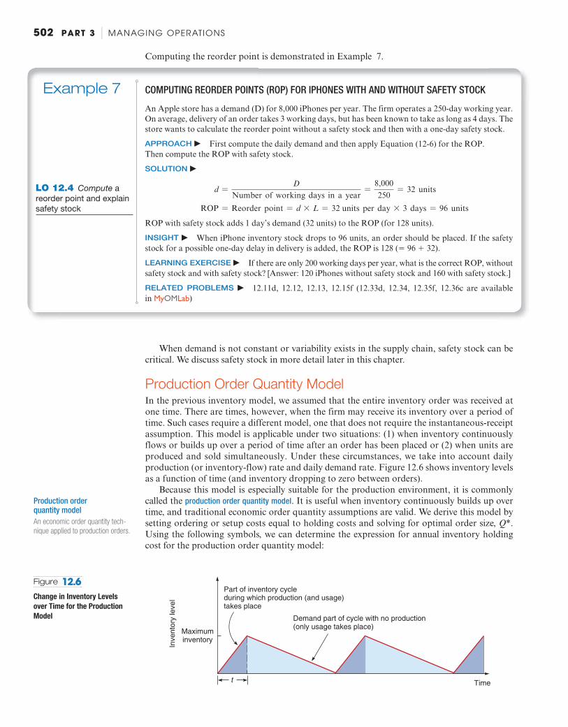
Production Order Quantity Model In the previous inventory model, we assumed that the entire inventory order was received at one time. There are times, however, when the firm may receive its inventory over a period of time. Such cases require a different model, one that does not require the instantaneous-receipt assumption. This model is applicable under two situations: (1) when inventory continuously flows or builds up over a period of time after an order has been placed or (2) when units are produced and sold simultaneously. Under these circumstances, we take into account daily production (or inventory-flow) rate and daily demand rate. Figure 12.6 shows inventory levels as a function of time (and inventory dropping to zero between orders).
Because this model is especially suitable for the production environment, it is commonly called the production order quantity model . It is useful when inventory continuously builds up over time, and traditional economic order quantity assumptions are valid. We derive this model by setting ordering or setup costs equal to holding costs and solving for optimal order size, Q *. Using the following symbols, we can determine the expression for annual inventory holding cost for the production order quantity model:
Production order quantity model
An economic order quantity tech-
nique applied to production orders.
t
Demand part of cycle with no production(only usage takes place)
Part of inventory cycleduring which production (and usage)takes place
Maximuminventory
Inve
ntor
y le
vel
Time
Figure 12.6
Change in Inventory Levels
over Time for the Production
Model
Example 7 COMPUTING REORDER POINTS (ROP) FOR IPHONES WITH AND WITHOUT SAFETY STOCK
An Apple store has a demand (D) for 8,000 iPhones per year. The firm operates a 250-day working year. On average, delivery of an order takes 3 working days, but has been known to take as long as 4 days. The store wants to calculate the reorder point without a safety stock and then with a one-day safety stock.
APPROACH c First compute the daily demand and then apply Equation (12-6) for the ROP. Then compute the ROP with safety stock.
SOLUTION c
d =D
Number of working days in a year=
8,000250
= 32 units
ROP = Reorder point = d * L = 32 units per day * 3 days = 96 units
ROP with safety stock adds 1 day’s demand (32 units) to the ROP (for 128 units).
INSIGHT c When iPhone inventory stock drops to 96 units, an order should be placed. If the safety stock for a possible one-day delay in delivery is added, the ROP is 128 (5 96 1 32).
LEARNING EXERCISE c If there are only 200 working days per year, what is the correct ROP, without safety stock and with safety stock? [Answer: 120 iPhones without safety stock and 160 with safety stock.]
RELATED PROBLEMS c 12.11d, 12.12, 12.13, 12.15f (12.33d, 12.34, 12.35f, 12.36c are available in MyOMLab)
LO 12.4 Compute a
reorder point and explain
safety stock
Computing the reorder point is demonstrated in Example 7 .
M16_HEIZ0422_12_SE_C12.indd 502M16_HEIZ0422_12_SE_C12.indd 502 05/11/15 5:03 PM05/11/15 5:03 PM
CHAPTER 12 | INVENTORY MANAGEMENT 503
Q = Number of units per order H = Holding cost per unit per year p = Daily production rate d = Daily demand rate, or usage rate t = Length of the production run in days
1. ¢Annual inventoryholding cost ≤ = (Average inventory level) * ¢ Holding cost
per unit per year≤
2. (Average inventory level) = (Maximum inventory level)>2
3. ¢ Maximuminventory level≤ = ¢Total production during
the production run ≤ - ¢ Total used duringthe production run≤
= pt - dt However, Q = total produced = pt, and thus t = Q>p. Therefore:
Maximum inventory level = p¢Qp ≤ - d¢Q
p ≤ = Q -dpQ
= Q¢1 -dp ≤
4. Annual inventory holding cost (or simply holding cost) 5
Maximum inventory level2
(H) =Q2C1 - ¢ d
p ≤ SH
Using this expression for holding cost and the expression for setup cost developed in the basic EOQ model, we solve for the optimal number of pieces per order by equating setup cost and holding cost:
Setup cost = (D>Q)S Holding cost = 12HQ [1 - (d>p)]
Set ordering cost equal to holding cost to obtain Q*p :
DQ
S = 12 HQ[1 - (d>p)]
Q2 =2DS
H[1 - (d>p)]
Q*p =A
2DSH[1 - (d>p)]
(12-7)
LO 12.5 Apply the
production order quantity
model
STUDENT TIP Note in Figure 12.6 that inventory
buildup is not instantaneous but
gradual. So the formula reduces
the average inventory and thus the
holding cost by the ratio of that
buildup.
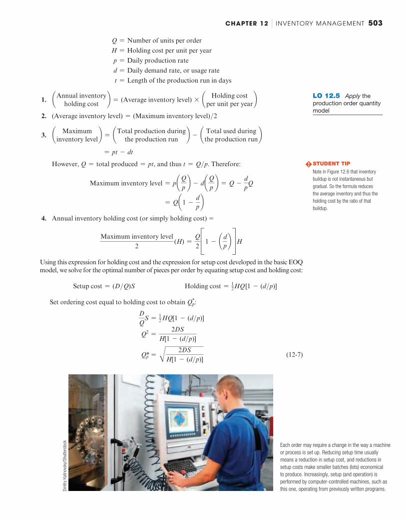
Each order may require a change in the way a machine
or process is set up. Reducing setup time usually
means a reduction in setup cost, and reductions in
setup costs make smaller batches (lots) economical
to produce. Increasingly, setup (and operation) is
performed by computer-controlled machines, such as
this one, operating from previously written programs. Dm
itry
Kal
inov
sky/
Shu
tter
stoc
k
M16_HEIZ0422_12_SE_C12.indd 503M16_HEIZ0422_12_SE_C12.indd 503 05/11/15 5:03 PM05/11/15 5:03 PM

504 PART 3 | MANAGING OPERATIONS
In Example 8 , we use the above equation, Q*p, to solve for the optimum order or production
quantity when inventory is consumed as it is produced.
Example 8 A PRODUCTION ORDER QUANTITY MODEL
Nathan Manufacturing, Inc., makes and sells specialty hubcaps for the retail automobile aftermarket. Nathan’s forecast for its wire-wheel hubcap is 1,000 units next year, with an average daily demand of 4 units. However, the production process is most efficient at 8 units per day. So the company produces 8 per day but uses only 4 per day. The company wants to solve for the optimum number of units per order. ( Note: This plant schedules production of this hubcap only as needed, during the 250 days per year the shop operates.)
APPROACH c Gather the cost data and apply Equation (12-7):
Annual demand = D = 1,000 units Setup costs = S = +10 Holding cost = H = +0.50 per unit per year Daily production rate = p = 8 units daily Daily demand rate = d = 4 units daily
SOLUTION c
Q*p =A
2DSH31 - (d>p)4
Q*p = A2(1,000)(10)
0.5031 - (4>8)4
=A
20,0000.50(1>2)
= 280,000 = 282.8 hubcaps, or 283 hubcaps
INSIGHT c The difference between the production order quantity model and the basic EOQ model is that the effective annual holding cost per unit is reduced in the production order quantity model because the entire order does not arrive at once.
LEARNING EXERCISE c If Nathan can increase its daily production rate from 8 to 10, how does Q*pchange? [Answer: Q*p 5 258.]
RELATED PROBLEMS c 12.18, 12.19, 12.20, 12.30 (12.37 is available in MyOMLab)
EXCEL OM Data File Ch12Ex8.xls can be found in MyOMLab.
ACTIVE MODEL 12.2 This example is further illustrated in Active Model 12.2 in MyOMLab.
You may want to compare this solution with the answer in Example 3 , which had identical D , S , and H values. Eliminating the instantaneous-receipt assumption, where p 5 8 and d 5 4, resulted in an increase in Q * from 200 in Example 3 to 283 in Example 8 . This increase in Q * occurred because holding cost dropped from $.50 to [$.50 3 (1 2 d Y p )], making a larger order quantity optimal. Also note that:
d = 4 =D
Number of days the plant is in operation=
1,000250
We can also calculate Q*p when annual data are available. When annual data are used, we can express Q*p as:
Q*p =
H
2DS
H¢1 -Annual demand rate
Annual production rate≤
(12-8)
M16_HEIZ0422_12_SE_C12.indd 504M16_HEIZ0422_12_SE_C12.indd 504 05/11/15 5:04 PM05/11/15 5:04 PM

CHAPTER 12 | INVENTORY MANAGEMENT 505
Quantity Discount Models Quantity discounts appear everywhere—you cannot go into a grocery store without seeing them on nearly every shelf. In fact, researchers have found that most companies either offer or receive quantity discounts for at least some of the products that they sell or purchase. A quantity discount is simply a reduced price ( P ) for an item when it is purchased in larger quantities. A typical quantity discount schedule appears in Table 12.2 . As can be seen in the table, the normal price of the item is $100. When 120 to 1,499 units are ordered at one time, the price per unit drops to $98; when the quantity ordered at one time is 1,500 units or more, the price is $96 per unit. The 120 quantity and the 1,500 quantity are called price-break quan-tities because they represent the first order amount that would lead to a new lower price. As always, management must decide when and how much to order. However, given these quan-tity discounts, how does the operations manager make these decisions?
As with other inventory models, the objective is to minimize total cost. Because the unit cost for the second discount in Table 12.2 is the lowest, you may be tempted to order 1,500 units. Placing an order for that quantity, however, even with the greatest discount price, may not minimize total inventory cost. This is because holding cost increases. Thus, the major trade-off when considering quantity discounts is between reduced product cost and increased holding cost . When we include the cost of the product, the equation for the total annual inventory cost can be calculated as follows:
Total annual cost 5 Annual setup (ordering) cost 1 Annual holding cost 1 Annual product cost,
or
TC =DQ
S +Q2
IP + PD (12-9)
where Q 5 Quantity ordered D 5 Annual demand in units S 5 Setup or ordering cost per order P 5 Price per unit I 5 Holding cost per unit per year expressed as a percent of price P
Note that holding cost is IP instead of H as seen in the regular EOQ model. Because the price of the item is a factor in annual holding cost, we do not assume that the holding cost is a constant when the price per unit changes for each quantity discount. Thus, it is common to express the holding cost as a percent ( I ) of unit price ( P ) when evaluating costs of quantity discount schedules.
The EOQ formula (12-1) is modified for the quantity discount problem as follows:
Q* =A
2DSIP
(12-10)
The solution procedure uses the concept of a feasible EOQ . An EOQ is feasible if it lies in the quantity range that leads to the same price P used to compute it in Equation (12-10). For ex-ample, suppose that D 5 5,200, S 5 $200, and I 5 28%. Using Table 12.2 and Equation (12-10), the EOQ for the $96 price equals 22(5,200)(200)>[(.28)(96)] = 278 units. Because 278 , 1,500 (the price-break quantity needed to receive the $96 price), the EOQ for the $96 price is not feasible . On the other hand, the EOQ for the $98 price equals 275 units. This amount is feasible because if 275 units were actually ordered, the firm would indeed receive the $98 purchase price.
Quantity discount
A reduced price for items
purchased in large quantities.
LO 12.6 Explain and
use the quantity discount
model
TABLE 12.2 A Quantity Discount Schedule
PRICE RANGE QUANTITY ORDERED PRICE PER UNIT P
Initial price 1–119 $100
Discount price 1 120–1,499 $ 98
Discount price 2 1,500 and over $ 96
M16_HEIZ0422_12_SE_C12.indd 505M16_HEIZ0422_12_SE_C12.indd 505 05/11/15 5:04 PM05/11/15 5:04 PM
506 PART 3 | MANAGING OPERATIONS
Now we have to determine the quantity that will minimize the total annual inventory cost. Because there are a few discounts, this process involves two steps. In Step 1, we identify all possible order quantities that could be the best solution. In Step 2, we calculate the total cost of all possible best order quantities, and the least expensive order quantity is selected.
Solution Procedure
STEP 1: Starting with the lowest possible purchase price in a quantity discount schedule and working toward the highest price, keep calculating Q* from Equation (12-10) until the fi rst feasible EOQ is found. The fi rst feasible EOQ is a possible best order quan-tity, along with all price-break quantities for all lower prices.
STEP 2: Calculate the total annual cost TC using Equation (12-9) for each of the possible best order quantities determined in Step 1. Select the quantity that has the lowest total cost.
Note that no quantities need to be considered for any prices greater than the first feasible EOQ found in Step 1. This occurs because if an EOQ for a given price is feasible, then the EOQ for any higher price cannot lead to a lower cost ( TC is guaranteed to be higher).
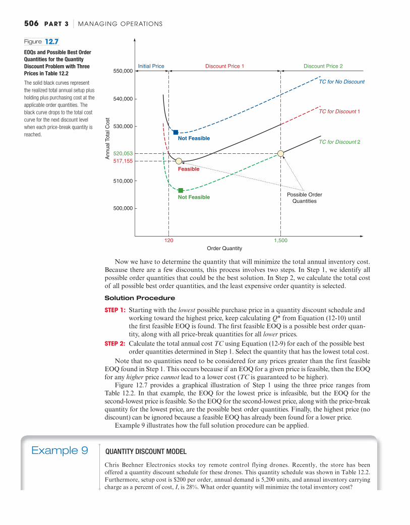
Figure 12.7 provides a graphical illustration of Step 1 using the three price ranges from Table 12.2 . In that example, the EOQ for the lowest price is infeasible, but the EOQ for the second-lowest price is feasible. So the EOQ for the second-lowest price, along with the price-break quantity for the lowest price, are the possible best order quantities. Finally, the highest price (no discount) can be ignored because a feasible EOQ has already been found for a lower price.
Example 9 illustrates how the full solution procedure can be applied.
Ann
ual T
otal
Cos
t
550,000
540,000
530,000
520,053517,155
510,000
500,000
120 1,500
Order Quantity
Not Feasible Possible OrderQuantities
TC for Discount 2
TC for Discount 1
Initial Price Discount Price 1 Discount Price 2
TC for No Discount
Not Feasible
Feasible
Figure 12.7
EOQs and Possible Best Order
Quantities for the Quantity
Discount Problem with Three
Prices in Table 12.2
The solid black curves represent
the realized total annual setup plus
holding plus purchasing cost at the
applicable order quantities. The
black curve drops to the total cost
curve for the next discount level
when each price-break quantity is
reached.
Example 9 QUANTITY DISCOUNT MODEL
Chris Beehner Electronics stocks toy remote control flying drones. Recently, the store has been offered a quantity discount schedule for these drones. This quantity schedule was shown in Table 12.2 . Furthermore, setup cost is $200 per order, annual demand is 5,200 units, and annual inventory carrying charge as a percent of cost, I , is 28%. What order quantity will minimize the total inventory cost?
M16_HEIZ0422_12_SE_C12.indd 506M16_HEIZ0422_12_SE_C12.indd 506 05/11/15 5:04 PM05/11/15 5:04 PM
CHAPTER 12 | INVENTORY MANAGEMENT 507
APPROACH c We will follow the two steps just outlined for the quantity discount model.
SOLUTION c First we calculate the Q * for the lowest possible price of $96, as we did earlier:
Q*$96 =A
2(5,200)($200)(.28)($96)
= 278 flying drones per order
Because 278 , 1,500, this EOQ is infeasible for the $96 price. So now we calculate Q * for the next-higher price of $98:
Q*$98 =A
2(5,200)($200)(.28)($98)
= 275 flying drones per order
Because 275 is between 120 and 1,499 units, this EOQ is feasible for the $98 price. Thus, the possible best order quantities are 275 (the first feasible EOQ) and 1,500 (the price-break quantity for the lower price of $96). We need not bother to compute Q * for the initial price of $100 because we found a feasible EOQ for a lower price.
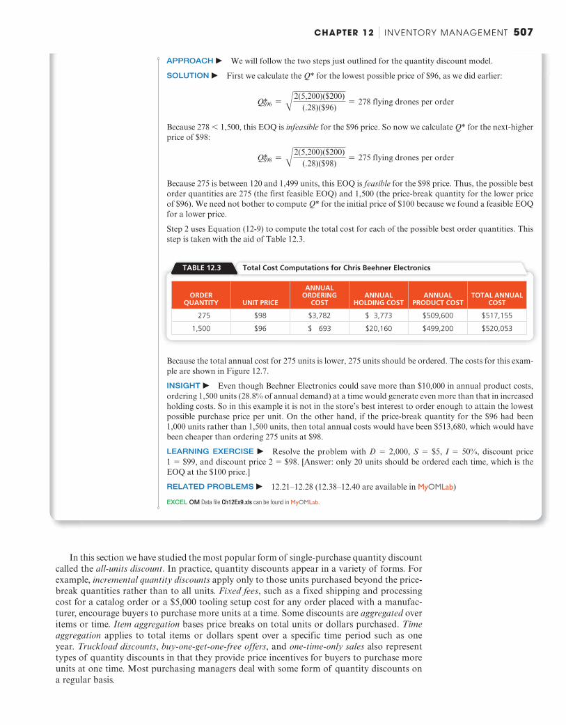
Step 2 uses Equation (12-9) to compute the total cost for each of the possible best order quantities. This step is taken with the aid of Table 12.3 .
TABLE 12.3 Total Cost Computations for Chris Beehner Electronics
ORDER QUANTITY UNIT PRICE
ANNUAL ORDERING
COSTANNUAL
HOLDING COSTANNUAL
PRODUCT COSTTOTAL ANNUAL
COST
275 $98 $3,782 $ 3,773 $509,600 $517,155
1,500 $96 $ 693 $20,160 $499,200 $520,053
Because the total annual cost for 275 units is lower, 275 units should be ordered. The costs for this exam-ple are shown in Figure 12.7 .
INSIGHT c Even though Beehner Electronics could save more than $10,000 in annual product costs, ordering 1,500 units (28.8% of annual demand) at a time would generate even more than that in increased holding costs. So in this example it is not in the store’s best interest to order enough to attain the lowest possible purchase price per unit. On the other hand, if the price-break quantity for the $96 had been 1,000 units rather than 1,500 units, then total annual costs would have been $513,680, which would have been cheaper than ordering 275 units at $98.
LEARNING EXERCISE c Resolve the problem with D 5 2,000, S 5 $5, I 5 50%, discount price 1 5 $99, and discount price 2 5 $98. [Answer: only 20 units should be ordered each time, which is the EOQ at the $100 price.]
RELATED PROBLEMS c 12.21–12.28 (12.38–12.40 are available in MyOMLab)
EXCEL OM Data file Ch12Ex9.xls can be found in MyOMLab.
In this section we have studied the most popular form of single-purchase quantity discount called the all-units discount . In practice, quantity discounts appear in a variety of forms. For example, i ncremental quantity discounts apply only to those units purchased beyond the price-break quantities rather than to all units. Fixed fees , such as a fixed shipping and processing cost for a catalog order or a $5,000 tooling setup cost for any order placed with a manufac-turer, encourage buyers to purchase more units at a time. Some discounts are aggregated over items or time. Item aggregation bases price breaks on total units or dollars purchased. Time aggregation applies to total items or dollars spent over a specific time period such as one year. Truckload discounts , buy-one-get-one-free offers , and one-time-only sales also represent types of quantity discounts in that they provide price incentives for buyers to purchase more units at one time. Most purchasing managers deal with some form of quantity discounts on a regular basis.
M16_HEIZ0422_12_SE_C12.indd 507M16_HEIZ0422_12_SE_C12.indd 507 05/11/15 5:04 PM05/11/15 5:04 PM

508 PART 3 | MANAGING OPERATIONS
Probabilistic Models and Safety Stock All the inventory models we have discussed so far make the assumption that demand for a product is constant and certain. We now relax this assumption. The following inventory mod-els apply when product demand is not known but can be specified by means of a probability distribution. These types of models are called probabilistic models . Probabilistic models are a real-world adjustment because demand and lead time won’t always be known and constant.
An important concern of management is maintaining an adequate service level in the face of uncertain demand. The service level is the complement of the probability of a stockout. For instance, if the probability of a stockout is 0.05, then the service level is .95. Uncertain demand raises the possibility of a stockout. One method of reducing stockouts is to hold extra units in inventory. As we noted earlier such inventory is referred to as safety stock. Safety stock in-volves adding a number of units as a buffer to the reorder point. As you recall:
Reorder point = ROP = d * L
where d 5 Daily demand L 5 Order lead time, or number of working days it takes to deliver an order
The inclusion of safety stock ( ss ) changed the expression to:
ROP = d * L + ss (12-11)
The amount of safety stock maintained depends on the cost of incurring a stockout and the cost of holding the extra inventory. Annual stockout cost is computed as follows:
Annual stockout costs = The sum of the units short for each demand level
* The probability of that demand level * The stockout cost>unit* The number of orders per year
(12-12)
Example 10 illustrates this concept.
Probabilistic model
A statistical model applicable
when product demand or any
other variable is not known but
can be specified by means of a
probability distribution.
Service level
The probability that demand will
not be greater than supply during
lead time. It is the complement of
the probability of a stockout.
Example 10 DETERMINING SAFETY STOCK WITH PROBABILISTIC DEMAND AND CONSTANT LEAD TIME
David Rivera Optical has determined that its reorder point for eyeglass frames is 50 (d * L) units. Its carrying cost per frame per year is $5, and stockout (or lost sale) cost is $40 per frame. The store has experienced the following probability distribution for inventory demand during the lead time (reorder period). The optimum number of orders per year is six.
NUMBER OF UNITS PROBABILITY
30 .2
40 .2
ROP S 50 .3
60 .2
70 .1
1.0
How much safety stock should David Rivera keep on hand?
APPROACH c The objective is to find the amount of safety stock that minimizes the sum of the addi-tional inventory holding costs and stockout costs. The annual holding cost is simply the holding cost per unit multiplied by the units added to the ROP. For example, a safety stock of 20 frames, which implies that the new ROP, with safety stock, is 70 (5 50 1 20), raises the annual carrying cost by $5(20) 5 $100.
However, computing annual stockout cost is more interesting. For any level of safety stock, stockout cost is the expected cost of stocking out. We can compute it, as in Equation (12-12), by multiplying the number of frames short (Demand – ROP) by the probability of demand at that level, by the stockout cost, by the number of times per year the stockout can occur (which in our case is the number of orders per year). Then we add stockout costs for each possible stockout level for a given ROP. 4
M16_HEIZ0422_12_SE_C12.indd 508M16_HEIZ0422_12_SE_C12.indd 508 05/11/15 5:04 PM05/11/15 5:04 PM

CHAPTER 12 | INVENTORY MANAGEMENT 509
SOLUTION c We begin by looking at zero safety stock. For this safety stock, a shortage of 10 frames will occur if demand is 60, and a shortage of 20 frames will occur if the demand is 70. Thus the stockout costs for zero safety stock are:
(10 frames short) (.2) (+40 per stockout) (6 possible stockouts per year)
+ (20 frames short) (.1) (+40)(6) = +960
The following table summarizes the total costs for each of the three alternatives:
SAFETY STOCK
ADDITIONAL HOLDING COST STOCKOUT COST
TOTAL COST
20 (20) ($5) 5 $100 $ 0 $100
10 (10) ($5) 5 $ 50 (10) (.1) ($40) (6) 5 $240 $290
0 $ 0 (10) (.2) ($40) (6) 1 (20) (.1) ($40) (6) 5 $960 $960
The safety stock with the lowest total cost is 20 frames. Therefore, this safety stock changes the reorder point to 50 1 20 5 70 frames.
INSIGHT c The optical company now knows that a safety stock of 20 frames will be the most economi-cal decision.
LEARNING EXERCISE c David Rivera’s holding cost per frame is now estimated to be $20, while the stockout cost is $30 per frame. Does the reorder point change? [Answer: Safety stock 5 10 now, with a total cost of $380, which is the lowest of the three. ROP 5 60 frames.]
RELATED PROBLEMS c 12.43, 12.44, 12.45
When it is difficult or impossible to determine the cost of being out of stock, a manager may decide to follow a policy of keeping enough safety stock on hand to meet a prescribed customer service level. For instance, Figure 12.8 shows the use of safety stock when demand (for hospital resuscitation kits) is probabilistic. We see that the safety stock in Figure 12.8 is 16.5 units, and the reorder point is also increased by 16.5.
The manager may want to define the service level as meeting 95% of the demand (or, con-versely, having stockouts only 5% of the time). Assuming that demand during lead time (the reorder period) follows a normal curve, only the mean and standard deviation are needed to define the inventory requirements for any given service level. Sales data are usually adequate for computing the mean and standard deviation. Example 11 uses a normal curve with a known mean (m) and standard deviation (s) to determine the reorder point and safety stock necessary
ROP = 350 + safety stock of 16.5 = 366.5
Expected demand during lead time (350 kits)
Safety stock
Normal distribution probability of demand during lead time
Mean demand during lead time
Maximum demand satisfied during lead time
Minimum demand during lead time
ROP(reorder point)
Inve
ntor
y le
vel
Leadtime
Time0
Receiveorder
Placeorder
16.5 units
Risk of stockout
Figure 12.8
Probabilistic Demand for
a Hospital Item
Expected number of kits needed
during lead time is 350, but for
a 95% service level, the reorder
point should be raised to 366.5.
M16_HEIZ0422_12_SE_C12.indd 509M16_HEIZ0422_12_SE_C12.indd 509 05/11/15 5:04 PM05/11/15 5:04 PM
510 PART 3 | MANAGING OPERATIONS
for a 95% service level. We use the following formula:
ROP = Expected demand during lead time + ZsdLT (12-13)
where Z 5 Number of standard deviations s dLT 5 Standard deviation of demand during lead time
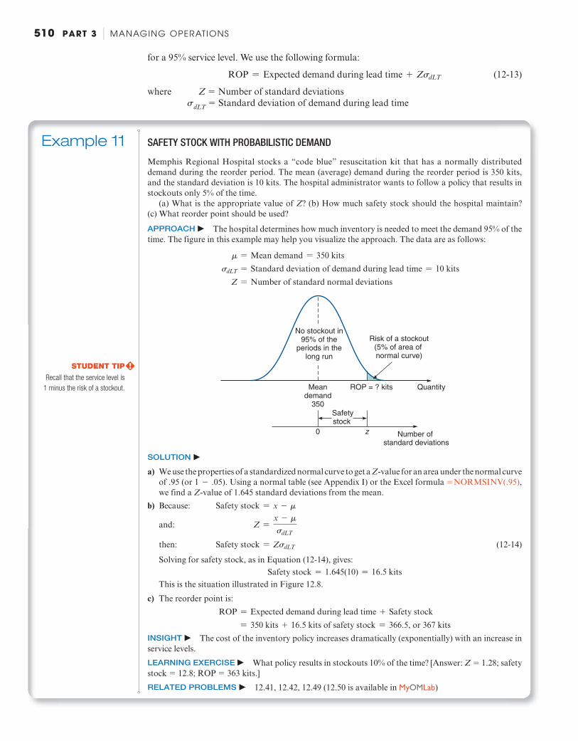
Example 11 SAFETY STOCK WITH PROBABILISTIC DEMAND
Memphis Regional Hospital stocks a “code blue” resuscitation kit that has a normally distributed demand during the reorder period. The mean (average) demand during the reorder period is 350 kits, and the standard deviation is 10 kits. The hospital administrator wants to follow a policy that results in stockouts only 5% of the time.
(a) What is the appropriate value of Z ? (b) How much safety stock should the hospital maintain? (c) What reorder point should be used?
APPROACH c The hospital determines how much inventory is needed to meet the demand 95% of the time. The figure in this example may help you visualize the approach. The data are as follows:
m = Mean demand = 350 kits sdLT = Standard deviation of demand during lead time = 10 kits Z = Number of standard normal deviations
Meandemand
350
ROP = ? kits Quantity
0 z
Safetystock
Number of standard deviations
Risk of a stockout(5% of area of normal curve)
No stockout in95% of the
periods in thelong run
SOLUTION c
a) We use the properties of a standardized normal curve to get a Z -value for an area under the normal curve of .95 (or 1 - .05). Using a normal table (see Appendix I ) or the Excel formula 5 NORMSINV(.95) , we find a Z -value of 1.645 standard deviations from the mean.
b) Because: Safety stock = x - m
and: Z =x - m
sdLT
then: Safety stock = ZsdLT (12-14)
Solving for safety stock, as in Equation (12-14), gives: Safety stock = 1.645(10) = 16.5 kits
This is the situation illustrated in Figure 12.8 .
c) The reorder point is: ROP = Expected demand during lead time + Safety stock = 350 kits + 16.5 kits of safety stock = 366.5, or 367 kits
INSIGHT c The cost of the inventory policy increases dramatically (exponentially) with an increase in service levels.
LEARNING EXERCISE c What policy results in stockouts 10% of the time? [Answer: Z 5 1.28; safety stock 5 12.8; ROP 5 363 kits.]
RELATED PROBLEMS c 12.41, 12.42, 12.49 (12.50 is available in MyOMLab)
STUDENT TIP Recall that the service level is
1 minus the risk of a stockout.
M16_HEIZ0422_12_SE_C12.indd 510M16_HEIZ0422_12_SE_C12.indd 510 05/11/15 5:04 PM05/11/15 5:04 PM
CHAPTER 12 | INVENTORY MANAGEMENT 511
Other Probabilistic Models Equations (12-13) and (12-14) assume that both an estimate of expected demand during lead times and its standard deviation are available. When data on lead time demand are not avail-able, the preceding formulas cannot be applied. However, three other models are available. We need to determine which model to use for three situations:
1. Demand is variable and lead time is constant 2. Lead time is variable and demand is constant 3. Both demand and lead time are variable
All three models assume that demand and lead time are independent variables. Note that our examples use days, but weeks can also be used. Let us examine these three situations sepa-rately, because a different formula for the ROP is needed for each.
Demand Is Variable and Lead Time Is Constant (See Example 12 .) When only the demand is variable , then: 5
ROP = (Average daily demand * Lead time in days) + ZsdLT (12-15)
where s dLT 5 Standard deviation of demand during lead time 5 sd2Lead time and s d 5 Standard deviation of demand per day
LO 12.7 Understand
service levels and
probabilistic inventory
models
Example 12 ROP FOR VARIABLE DEMAND AND CONSTANT LEAD TIME
The average daily demand for Lenovo laptop computers at a Circuit Town store is 15, with a standard deviation of 5 units. The lead time is constant at 2 days. Find the reorder point if management wants a 90% service level (i.e., risk stockouts only 10% of the time). How much of this is safety stock?
APPROACH c Apply Equation (12-15) to the following data:
Average daily demand (normally distributed) 5 15
Lead time in days (constant) 5 2
Standard deviation of daily demand 5 s d 5 5
Service level 5 90%
SOLUTION c From the normal table ( Appendix I ) or the Excel formula = NORMSINV(.90) , we derive a Z -value for 90% of 1.28. Then:
ROP = (15 units * 2 days) + Zsd2Lead time = 30 + 1.28(5) (22) = 30 + 1.28(5) (1.41) = 30 + 9.02 = 39.02 _ 39
Thus, safety stock is about 9 Lenovo computers.
INSIGHT c The value of Z depends on the manager’s stockout risk level. The smaller the risk, the higher the Z .
LEARNING EXERCISE c If the Circuit Town manager wants a 95% service level, what is the new ROP? [Answer: ROP 5 41.63, or 42.]
RELATED PROBLEM c 12.46
Lead Time Is Variable and Demand Is Constant When the demand is constant and only the lead time is variable , then:
ROP = (Daily demand * Average lead time in days) + Z * Daily demand * sLT (12-16)
where s LT 5 Standard deviation of lead time in days
M16_HEIZ0422_12_SE_C12.indd 511M16_HEIZ0422_12_SE_C12.indd 511 05/11/15 5:04 PM05/11/15 5:04 PM
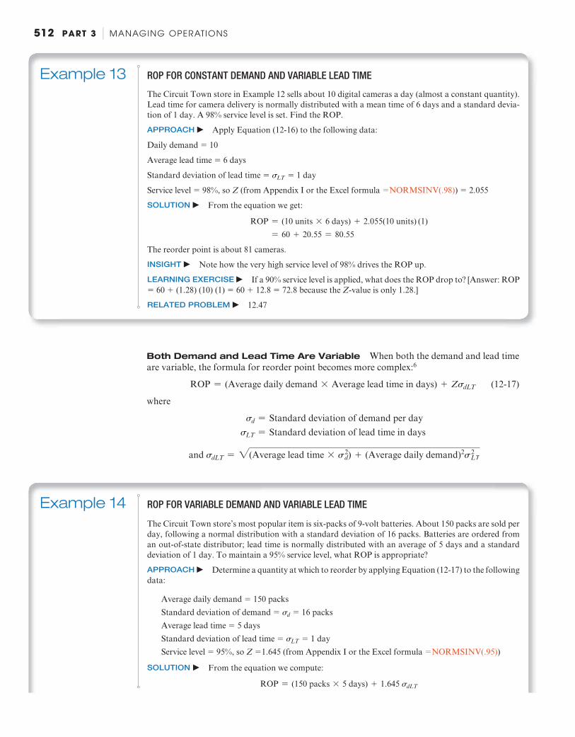
512 PART 3 | MANAGING OPERATIONS
Example 13 ROP FOR CONSTANT DEMAND AND VARIABLE LEAD TIME
The Circuit Town store in Example 12 sells about 10 digital cameras a day (almost a constant quantity). Lead time for camera delivery is normally distributed with a mean time of 6 days and a standard devia-tion of 1 day. A 98% service level is set. Find the ROP.
APPROACH c Apply Equation (12-16) to the following data:
Daily demand 5 10
Average lead time 5 6 days
Standard deviation of lead time 5 sLT 5 1 day
Service level 5 98%, so Z (from Appendix I or the Excel formula = NORMSINV(.98)) 5 2.055
SOLUTION c From the equation we get:
ROP = (10 units * 6 days) + 2.055(10 units) (1) = 60 + 20.55 = 80.55
The reorder point is about 81 cameras.
INSIGHT c Note how the very high service level of 98% drives the ROP up.
LEARNING EXERCISE c If a 90% service level is applied, what does the ROP drop to? [Answer: ROP 5 60 1 (1.28) (10) (1) 5 60 1 12.8 5 72.8 because the Z -value is only 1.28.]
RELATED PROBLEM c 12.47
Both Demand and Lead Time Are Variable When both the demand and lead time are variable, the formula for reorder point becomes more complex: 6
ROP = (Average daily demand * Average lead time in days) + ZsdLT (12-17)
where
sd = Standard deviation of demand per day sLT = Standard deviation of lead time in days
and sdLT = 2(Average lead time * sd 2) + (Average daily demand)2sLT
2
Example 14 ROP FOR VARIABLE DEMAND AND VARIABLE LEAD TIME
The Circuit Town store’s most popular item is six-packs of 9-volt batteries. About 150 packs are sold per day, following a normal distribution with a standard deviation of 16 packs. Batteries are ordered from an out-of-state distributor; lead time is normally distributed with an average of 5 days and a standard deviation of 1 day. To maintain a 95% service level, what ROP is appropriate?
APPROACH c Determine a quantity at which to reorder by applying Equation (12-17) to the following data:
Average daily demand 5 150 packs Standard deviation of demand 5 sd 5 16 packs Average lead time 5 5 days Standard deviation of lead time 5 sLT 5 1 day Service level 5 95%, so Z 51.645 (from Appendix I or the Excel formula = NORMSINV(.95))
SOLUTION c From the equation we compute:
ROP = (150 packs * 5 days) + 1.645 sdLT
M16_HEIZ0422_12_SE_C12.indd 512M16_HEIZ0422_12_SE_C12.indd 512 05/11/15 5:04 PM05/11/15 5:04 PM
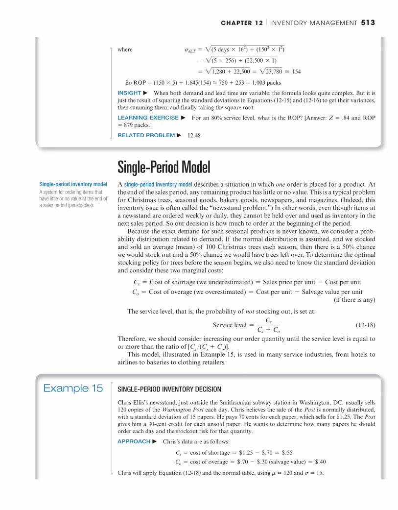
CHAPTER 12 | INVENTORY MANAGEMENT 513
where sdLT = 2(5 days * 162) + (1502 * 12)
= 2(5 * 256) + (22,500 * 1)
= 21,280 + 22,500 = 223,780 _ 154
So ROP 5 (150 3 5) 1 1.645(154) > 750 1 253 5 1,003 packs
INSIGHT c When both demand and lead time are variable, the formula looks quite complex. But it is just the result of squaring the standard deviations in Equations (12-15) and (12-16) to get their variances, then summing them, and finally taking the square root.
LEARNING EXERCISE c For an 80% service level, what is the ROP? [Answer: Z 5 .84 and ROP 5 879 packs.]
RELATED PROBLEM c 12.48
Single-Period Model A single-period inventory model describes a situation in which one order is placed for a product. At the end of the sales period, any remaining product has little or no value. This is a typical problem for Christmas trees, seasonal goods, bakery goods, newspapers, and magazines. (Indeed, this inventory issue is often called the “newsstand problem.”) In other words, even though items at a newsstand are ordered weekly or daily, they cannot be held over and used as inventory in the next sales period. So our decision is how much to order at the beginning of the period.
Because the exact demand for such seasonal products is never known, we consider a prob-ability distribution related to demand. If the normal distribution is assumed, and we stocked and sold an average (mean) of 100 Christmas trees each season, then there is a 50% chance we would stock out and a 50% chance we would have trees left over. To determine the optimal stocking policy for trees before the season begins, we also need to know the standard deviation and consider these two marginal costs:
Cs = Cost of shortage (we underestimated) = Sales price per unit - Cost per unit Co = Cost of overage (we overestimated) = Cost per unit - Salvage value per unit
(if there is any)
The service level, that is, the probability of not stocking out, is set at:
Service level =Cs
Cs + Co (12-18)
Therefore, we should consider increasing our order quantity until the service level is equal to or more than the ratio of [ C s Y( C s 1 C o )].
This model, illustrated in Example 15 , is used in many service industries, from hotels to airlines to bakeries to clothing retailers.
Single-period inventory model
A system for ordering items that
have little or no value at the end of
a sales period (perishables).
Example 15 SINGLE-PERIOD INVENTORY DECISION
Chris Ellis’s newsstand, just outside the Smithsonian subway station in Washington, DC, usually sells 120 copies of the Washington Post each day. Chris believes the sale of the Post is normally distributed, with a standard deviation of 15 papers. He pays 70 cents for each paper, which sells for $1.25. The Post gives him a 30-cent credit for each unsold paper. He wants to determine how many papers he should order each day and the stockout risk for that quantity.
APPROACH c Chris’s data are as follows:
Cs = cost of shortage = +1.25 - +.70 = +.55 Co = cost of overage = +.70 - +.30 (salvage value) = +.40
Chris will apply Equation (12-18) and the normal table, using m 5 120 and s 5 15.
M16_HEIZ0422_12_SE_C12.indd 513M16_HEIZ0422_12_SE_C12.indd 513 05/11/15 5:04 PM05/11/15 5:04 PM

514 PART 3 | MANAGING OPERATIONS
Fixed-quantity ( Q ) system
An ordering system with the same
order amount each time.
SOLUTION c a) Service level 5
Cs
Cs + Co=
.55.55 + .40
=.55.95
= .579
b) Chris needs to find the Z score for his normal distribution that yields a probability of .579.
o = 120
u = 15 copies
Servicelevel
57.9%
Optimal stocking level
So 57.9% of the area under the normal curve must be to the left of the optimal stocking level.
c) Using Appendix I or the Excel formula = NORMSINV(.578) , for an area of .578, the Z value > .195.
Then, the optimal stocking level = 120 copies + (.195) (s) = 120 + (.195) (15) = 120 + 3 = 123 papers
The stockout risk if Chris orders 123 copies of the Post each day is 1 2 Service level 5 1 2 .578 5 .422 5 42.2%.
INSIGHT c If the service level is ever under .50, Chris should order fewer than 120 copies per day.
LEARNING EXERCISE c How does Chris’s decision change if the Post changes its policy and offers no credit for unsold papers, a policy many publishers are adopting?
[Answer: Service level 5 .44, Z 5 2.15. Therefore, stock 120 1 (2.15)(15) 5 117.75, or 118 papers.]
RELATED PROBLEMS c 12.51, 12.52, 12.53
Fixed-Period ( P ) Systems The inventory models that we have considered so far are fixed-quantity, or Q , systems . That is, the same fixed amount is added to inventory every time an order for an item is placed. We saw that orders are event triggered. When inventory decreases to the reorder point (ROP), a new order for Q units is placed.
To use the fixed-quantity model, inventory must be continuously monitored. 7 This requires a perpetual inventory system . Every time an item is added to or withdrawn from inventory, records must be updated to determine whether the ROP has been reached. In a fixed-period system (also called a periodic review, or P system ), on the other hand, inventory is ordered at the end of a given period. Then, and only then, is on-hand inventory counted. Only the amount necessary to bring total inventory up to a prespecified target level ( T ) is ordered. Figure 12.9 illustrates this concept.
Fixed-period systems have several of the same assumptions as the basic EOQ fixed- quantity system: ◆ The only relevant costs are the
ordering and holding costs. ◆ Lead times are known and constant. ◆ Items are independent of one another. The downward-sloped lines in Figure 12.9 again represent on-hand inventory levels. But now, when the time between orders ( P ) passes, we place an order to raise inventory up to the target quantity ( T ).
Perpetual inventory system
A system that keeps track of each
withdrawal or addition to inven-
tory continuously, so records are
always current.
Fixed-period ( P ) system
A system in which inventory orders
are made at regular time intervals.
P
Q1
Q2
Q3
Q4
P
P
On-
hand
inve
ntor
y
Time
Target quantity (T ) Figure 12.9
Inventory Level in a
Fixed-Period ( P ) System
Various amounts ( Q 1 , Q
2 , Q
3 ,
etc.) are ordered at regular time
intervals ( P ) based on the quantity
necessary to bring inventory up to
the target quantity ( T ).
M16_HEIZ0422_12_SE_C12.indd 514M16_HEIZ0422_12_SE_C12.indd 514 05/11/15 5:04 PM05/11/15 5:04 PM

CHAPTER 12 | INVENTORY MANAGEMENT 515
The amount ordered during the first period may be Q 1 , the second period Q 2 , and so on. The Q ivalue is the difference between current on-hand inventory and the target inventory level.
The advantage of the fixed-period system is that there is no physical count of inventory items after an item is withdrawn—this occurs only when the time for the next review comes up. This procedure is also convenient administratively.
A fixed-period (P) system is appropriate when vendors make routine (i.e., at fixed-time inter-val) visits to customers to take fresh orders or when purchasers want to combine orders to save ordering and transportation costs (therefore, they will have the same review period for similar in-ventory items). For example, a vending machine company may come to refill its machines every Tuesday. This is also the case at Anheuser-Busch, whose sales reps may visit a store every 5 days.
The disadvantage of the P system is that because there is no tally of inventory during the review period, there is the possibility of a stockout during this time. This scenario is possible if a large order draws the inventory level down to zero right after an order is placed. Therefore, a higher level of safety stock (as compared to a fixed-quantity system) needs to be maintained to provide protection against stockout during both the time between reviews and the lead time.
STUDENT TIP A fixed-period model potentially
orders a different quantity each time.
Summary Inventory represents a major investment for many firms. This investment is often larger than it should be because firms find it easier to have “just-in-case” inventory rather than “just-in-time” inventory. Inventories are of four types:
1. Raw material and purchased components 2. Work-in-process 3. Maintenance, repair, and operating (MRO)
4. Finished goods
In this chapter, we discussed independent inventory, ABC analysis, record accuracy, cycle counting, and inven-tory models used to control independent demands. The EOQ model, production order quantity model, and quantity discount model can all be solved using Excel, Excel OM, or POM for Windows software.
Key Terms
Raw material inventory (p. 490 ) Work-in-process (WIP) inventory (p. 490 ) Maintenance/repair/operating (MRO)
inventory (p. 490 ) Finished-goods inventory (p. 491 ) ABC analysis (p. 491 ) Cycle counting (p. 493 ) Shrinkage (p. 494 ) Pilferage (p. 494 )
Holding cost (p. 495 ) Ordering cost (p. 495 ) Setup cost (p. 496 ) Setup time (p. 496 ) Economic order quantity (EOQ)
model (p. 496 ) Robust (p. 500 ) Lead time (p. 501 ) Reorder point (ROP) (p. 501 )
Safety stock ( ss ) (p. 501 ) Production order quantity model (p. 502 ) Quantity discount (p. 505 ) Probabilistic model (p. 508 ) Service level (p. 508 ) Single-period inventory model (p. 513 ) Fixed-quantity ( Q ) system (p. 514 ) Perpetual inventory system (p. 514 ) Fixed-period ( P ) system (p. 514 )
Ethical Dilemma Wayne Hills Hospital in tiny Wayne, Nebraska, faces a problem common to large, urban hospitals as well as to small, remote ones like itself. That problem is deciding how much of each type of whole blood to keep in stock. Because blood is expensive and has a limited shelf life (up to 5 weeks under 1–6°C refrigeration), Wayne Hills naturally wants to keep its stock as low as possible. Unfortunately, past disasters such as a major tornado and a train wreck demonstrated that lives would be lost when not enough blood was available to handle massive needs. The hospital
administrator wants to set an 85% service level based on demand over the past decade. Discuss the implications of this decision. What is the hospital’s responsibility with regard to stocking lifesaving medicines with short shelf lives? How would you set the inventory level for a commodity such as blood?
Gin
asan
ders
/Fot
olia
Discussion Questions
1. Describe the four types of inventory. 2. With the advent of low-cost computing, do you see alterna-
tives to the popular ABC classifications? 3. What is the purpose of the ABC classification system? 4. Identify and explain the types of costs that are involved in an
inventory system.
5. Explain the major assumptions of the basic EOQ model. 6. What is the relationship of the economic order quantity to
demand? To the holding cost? To the setup cost? 7. Explain why it is not necessary to include product cost (price
or price times quantity) in the EOQ model, but the quantity discount model requires this information.
M16_HEIZ0422_12_SE_C12.indd 515M16_HEIZ0422_12_SE_C12.indd 515 05/11/15 5:04 PM05/11/15 5:04 PM
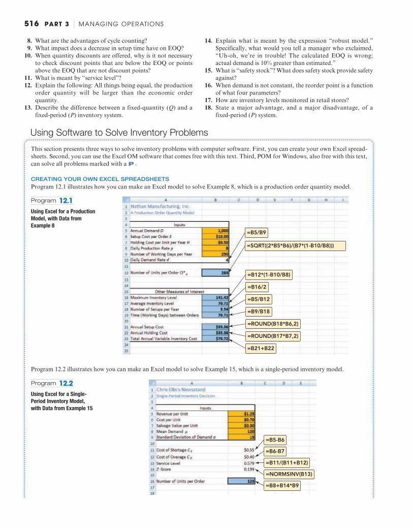
516 PART 3 | MANAGING OPERATIONS
8. What are the advantages of cycle counting? 9. What impact does a decrease in setup time have on EOQ?
10. When quantity discounts are offered, why is it not necessary to check discount points that are below the EOQ or points above the EOQ that are not discount points?
11. What is meant by “service level”? 12. Explain the following: All things being equal, the production
order quantity will be larger than the economic order quantity.
13. Describe the difference between a fixed-quantity ( Q ) and a fixed-period ( P ) inventory system.
14. Explain what is meant by the expression “robust model.” Specifically, what would you tell a manager who exclaimed, “Uh-oh, we’re in trouble! The calculated EOQ is wrong; actual demand is 10% greater than estimated.”
15. What is “safety stock”? What does safety stock provide safety against?
16. When demand is not constant, the reorder point is a function of what four parameters?
17. How are inventory levels monitored in retail stores? 18. State a major advantage, and a major disadvantage, of a
fixed-period ( P ) system.
This section presents three ways to solve inventory problems with computer software. First, you can create your own Excel spread-sheets. Second, you can use the Excel OM software that comes free with this text. Third, POM for Windows, also free with this text, can solve all problems marked with a P .
CREATING YOUR OWN EXCEL SPREADSHEETS Program 12.1 illustrates how you can make an Excel model to solve Example 8 , which is a production order quantity model.
=B5/B9
=SQRT((2*B5*B6)/(B7*(1-B10/B8)))
=B12*(1-B10/B8)
=B16/2
=B5/B12
=B9/B18
=ROUND(B18*B6,2)
=ROUND(B17*B7,2)
=B21+B22
Program 12.1
Using Excel for a Production
Model, with Data from
Example 8
Program 12.2 illustrates how you can make an Excel model to solve Example 15, which is a single-period inventory model.
=B5-B6
=B6-B7
=B11/(B11+B12)
=NORMSINV(B13)
=B8+B14*B9
Program 12.2
Using Excel for a Single-
Period Inventory Model,
with Data from Example 15
Using Software to Solve Inventory Problems
M16_HEIZ0422_12_SE_C12.indd 516M16_HEIZ0422_12_SE_C12.indd 516 05/11/15 5:04 PM05/11/15 5:04 PM

CHAPTER 12 | INVENTORY MANAGEMENT 517
The cumulative dollar volumes in columnG make sense only after the items havebeen sorted by dollar volume. Either usethe copy and sort button, or, to sort byhand, highlight cells A7 through E17 andthen use the Data and Sort commands.
Calculate the total dollarvolume for each item. = B8*C8 Calculate the percentage of
the grand total dollar volumefor each item. = E8/E18
= SUM(E8:E17)
= SUM($F$8:F8)
Enter the itemname or number,its sales volume,and the unit costin columns A, B,and C.
Program 12.3
Using Excel OM for an ABC Analysis, with Data from Example 1
X USING EXCEL OM Excel OM allows us to easily model inventory problems ranging from ABC analysis, to the basic EOQ model, to the production model, to quantity discount situations.
Program 12.3 shows the input data, selected formulas, and results for an ABC analysis, using data from Example 1 . After the data are entered, we use the Data and Sort Excel commands to rank the items from largest to smallest dollar volumes.
P USING POM FOR WINDOWS The POM for Windows Inventory module can also solve the entire EOQ family of problems. Please refer to Appendix IV for further details.
Solved Problems Virtual Office Hours help is available in MyOMLab.
SOLVED PROBLEM 12.1 David Alexander has compiled the following table of six items in inventory at Angelo Products, along with the unit cost and the annual demand in units:
IDENTIFICATION CODE UNIT COST ($)ANNUAL DEMAND
(UNITS)
XX1 5.84 1,200
B66 5.40 1,110
3CPO 1.12 896
33CP 74.54 1,104
R2D2 2.00 1,110
RMS 2.08 961
Use ABC analysis to determine which item(s) should be care-fully controlled using a quantitative inventory technique and which item(s) should not be closely controlled.
SOLUTION The item that needs strict control is 33CP, so it is an A item. Items that do not need to be strictly controlled are 3CPO, R2D2, and RMS; these are C items. The B items will be XX1 and B66.
CODE ANNUAL DOLLAR VOLUME 5 UNIT COST 3 DEMAND
XX1 $ 7,008.00
B66 $ 5,994.00
3CPO $ 1,003.52
33CP $82,292.16
R2D2 $ 2,220.00
RMS $ 1,998.88
Total cost 5 $100,516.56 70% of total cost 5 $70,347.92
SOLVED PROBLEM 12.2 The Warren W. Fisher Computer Corporation purchases 8,000 transistors each year as components in minicomputers. The unit cost of each transistor is $10, and the cost of carrying one tran-sistor in inventory for a year is $3. Ordering cost is $30 per order.
What are (a) the optimal order quantity, (b) the expected number of orders placed each year, and (c) the expected time between orders? Assume that Fisher operates on a 200-day working year.
M16_HEIZ0422_12_SE_C12.indd 517M16_HEIZ0422_12_SE_C12.indd 517 05/11/15 5:04 PM05/11/15 5:04 PM
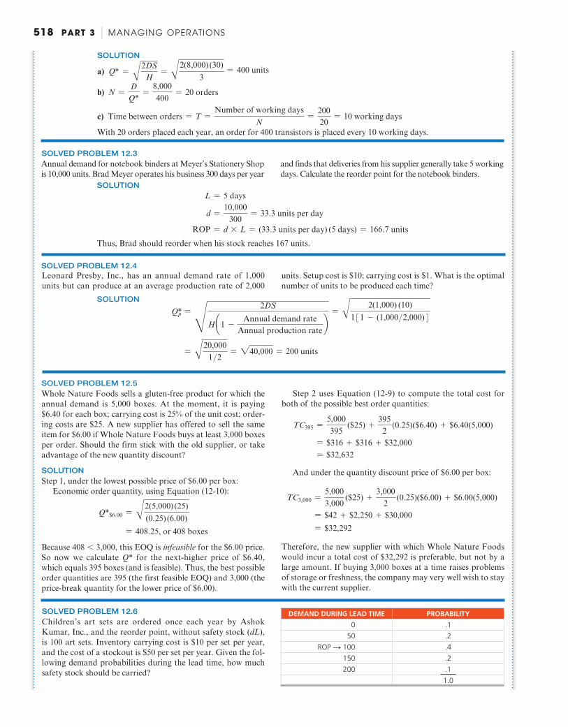
518 PART 3 | MANAGING OPERATIONS
SOLUTION
a) Q* =A
2DSH
= A2(8,000) (30)
3= 400 units
b) N =DQ*
=8,000400
= 20 orders
c) Time between orders = T =Number of working days
N=
20020
= 10 working days
With 20 orders placed each year, an order for 400 transistors is placed every 10 working days.
SOLVED PROBLEM 12.3 Annual demand for notebook binders at Meyer’s Stationery Shop is 10,000 units. Brad Meyer operates his business 300 days per year
and finds that deliveries from his supplier generally take 5 working days. Calculate the reorder point for the notebook binders.
SOLUTION L = 5 days
d =10,000
300= 33.3 units per day
ROP = d * L = (33.3 units per day) (5 days) = 166.7 units
Thus, Brad should reorder when his stock reaches 167 units.
SOLVED PROBLEM 12.4 Leonard Presby, Inc., has an annual demand rate of 1,000 units but can produce at an average production rate of 2,000
units. Setup cost is $10; carrying cost is $1. What is the optimal number of units to be produced each time?
SOLUTION
Q*p =
H
2DS
H¢1 -Annual demand rate
Annual production rate≤
= A2(1,000) (10)
131 - (1,000>2,000)4
= A20,000
1>2= 240,000 = 200 units
SOLVED PROBLEM 12.5 Whole Nature Foods sells a gluten-free product for which the annual demand is 5,000 boxes. At the moment, it is paying $6.40 for each box; carrying cost is 25% of the unit cost; order-ing costs are $25. A new supplier has offered to sell the same item for $6.00 if Whole Nature Foods buys at least 3,000 boxes per order. Should the firm stick with the old supplier, or take advantage of the new quantity discount?
SOLUTION Step 1, under the lowest possible price of $6.00 per box:
Economic order quantity, using Equation (12-10):
Q*$6.00 = A2(5,000) (25)(0.25) (6.00)
= 408.25, or 408 boxes
Because 408 , 3,000, this EOQ is infeasible for the $6.00 price. So now we calculate Q * for the next-higher price of $6.40, which equals 395 boxes (and is feasible). Thus, the best possible order quantities are 395 (the first feasible EOQ) and 3,000 (the price-break quantity for the lower price of $6.00).
Step 2 uses Equation (12-9) to compute the total cost for both of the possible best order quantities:
TC395 =5,000395
($25) +3952
(0.25)($6.40) + $6.40(5,000)
= $316 + $316 + $32,000 = $32,632
And under the quantity discount price of $6.00 per box:
TC3,000 =5,0003,000
($25) +3,000
2 (0.25)($6.00) + $6.00(5,000)
= $42 + $2,250 + $30,000 = $32,292
Therefore, the new supplier with which Whole Nature Foods would incur a total cost of $32,292 is preferable, but not by a large amount. If buying 3,000 boxes at a time raises problems of storage or freshness, the company may very well wish to stay with the current supplier.
SOLVED PROBLEM 12.6 Children’s art sets are ordered once each year by Ashok Kumar, Inc., and the reorder point, without safety stock ( dL ), is 100 art sets. Inventory carrying cost is $10 per set per year, and the cost of a stockout is $50 per set per year. Given the fol-lowing demand probabilities during the lead time, how much safety stock should be carried?
DEMAND DURING LEAD TIME PROBABILITY
0 .150 .2
ROP S 100 .4150 .2200 .1
1.0
M16_HEIZ0422_12_SE_C12.indd 518M16_HEIZ0422_12_SE_C12.indd 518 05/11/15 5:04 PM05/11/15 5:04 PM

CHAPTER 12 | INVENTORY MANAGEMENT 519
SOLUTION
INCREMENTAL COSTS
SAFETY STOCK CARRYING COST STOCKOUT COST TOTAL COST
0 0 50 3 (50 3 0.2 1 100 3 0.1) 5 1,000 $1,000
50 50 3 10 5 500 50 3 (0.1 3 50) 5 250 750
100 100 3 10 5 1,000 0 1,000
The safety stock that minimizes total incremental cost is 50 sets. The reorder point then becomes 100 sets 1 50 sets, or 150 sets.
SOLVED PROBLEM 12.7 What safety stock should Ron Satterfield Corporation maintain if mean sales are 80 during the reorder period, the
standard deviation is 7, and Ron can tolerate stockouts 10% of the time?
SOLUTION
o = 80udLT = 7
10% area under the normal curve
Safetystock
From Appendix I , Z at an area of .9 (or 1 2 .10) 5 1.28, and Equation (12-14): Safety stock = ZsdLT = 1.28(7) = 8.96 units, or 9 units
SOLVED PROBLEM 12.8 The daily demand for 52” flat-screen TVs at Sarah’s Discount Emporium is normally distributed, with an average of 5 and a standard deviation of 2 units. The lead time for receiving a ship-
SOLUTION The ROP for this variable demand and constant lead time model uses Equation (12-15):
ROP = (Average daily demand * Lead time in days) + ZsdLT
where sdLT = sd2Lead time So, with Z 5 1.645,
ROP = (5 * 10) + 1.645(2)210 = 50 + 10.4 = 60.4 _ 60 TVs, or rounded up to 61 TVs
The safety stock is 10.4, which can be rounded up to 11 TVs.
ment of new TVs is 10 days and is fairly constant. Determine the reorder point and safety stock for a 95% service level.
SOLVED PROBLEM 12.9 The demand at Arnold Palmer Hospital for a special-ized surgery pack is 60 per week, virtually every week. The lead time from McKesson, its main supplier, is normally
distributed, with a mean of 6 weeks for this product and a standard deviation of 2 weeks. A 90% weekly service level is desired. Find the ROP.
SOLUTION Here the demand is constant and lead time is variable, with data given in weeks, not days. We apply Equation (12-16):
ROP = (Weekly demand * Average lead time in weeks) + Z (Weekly demand) sLT where sLT = standard deviation of lead time in weeks = 2
So, with Z 5 1.28, for a 90% service level: ROP = (60 * 6) + 1.28(60) (2) = 360 + 153.6 = 513.6 _ 514 surgery packs
M16_HEIZ0422_12_SE_C12.indd 519M16_HEIZ0422_12_SE_C12.indd 519 05/11/15 5:04 PM05/11/15 5:04 PM

520 PART 3 | MANAGING OPERATIONS
Problems Note: PX means the problem may be solved with POM for Windows and/or Excel OM.
Problems 12.1–12.6 relate to Managing Inventory
• • 12.1 L. Houts Plastics is a large manufacturer of injection-molded plastics in North Carolina. An investigation of the com-pany’s manufacturing facility in Charlotte yields the information presented in the table below. How would the plant classify these items according to an ABC classification system? PX
L. Houts Plastics’ Charlotte Inventory Levels
ITEM CODE # AVERAGE INVENTORY (UNITS) VALUE ($/UNIT)
1289 400 3.75
2347 300 4.00
2349 120 2.50
2363 75 1.50
2394 60 1.75
2395 30 2.00
6782 20 1.15
7844 12 2.05
8210 8 1.80
8310 7 2.00
9111 6 3.00
• • 12.2 Boreki Enterprises has the following 10 items in inventory. Theodore Boreki asks you, a recent OM graduate, to divide these items into ABC classifications.
ITEM ANNUAL DEMAND COST/UNIT
A2 3,000 $ 50
B8 4,000 12
C7 1,500 45
D1 6,000 10
E9 1,000 20
F3 500 500
G2 300 1,500
H2 600 20
I5 1,750 10
J8 2,500 5
a) Develop an ABC classification system for the 10 items. b) How can Boreki use this information? c) Boreki reviews the classification and then places item A2 into
the A category. Why might he do so? PX
• • 12.3 Jean-Marie Bourjolly’s restaurant has the following inventory items that it orders on a weekly basis:
INVENTORY ITEM $ VALUE/CASE # ORDERED/WEEK
Ribeye steak 135 3
Lobster tail 245 3
Pasta 23 12
Salt 3 2
Napkins 12 2
Tomato sauce 23 11
French fries 43 32
INVENTORY ITEM $ VALUE/CASE # ORDERED/WEEK
Pepper 3 3
Garlic powder 11 3
Trash can liners 12 3
Table cloths 32 5
Fish fi lets 143 10
Prime rib roasts 166 6
Oil 28 2
Lettuce (case) 35 24
Chickens 75 14
Order pads 12 2
Eggs (case) 22 7
Bacon 56 5
Sugar 4 2
a) Which is the most expensive item, using annual dollar volume? b) Which are C items? c) What is the annual dollar volume for all 20 items? PX
• 12.4 Lindsay Electronics, a small manufacturer of elec-tronic research equipment, has approximately 7,000 items in its inventory and has hired Joan Blasco-Paul to manage its inven-tory. Joan has determined that 10% of the items in inventory are A items, 35% are B items, and 55% are C items. She would like to set up a system in which all A items are counted monthly (every 20 working days), all B items are counted quarterly (every 60 work-ing days), and all C items are counted semiannually (every 120 working days). How many items need to be counted each day?
Additional problems 12.5–12.6 are available in MyOMLab.
Problems 12.7–12.40 relate to Inventory Models for Independent Demand
• 12.7 William Beville’s computer training school, in Richmond, stocks workbooks with the following characteristics:
Demand D = 19,500 units>year Ordering cost S = +25>order Holding cost H = +4>unit>year
a) Calculate the EOQ for the workbooks. b) What are the annual holding costs for the workbooks? c) What are the annual ordering costs? PX
• 12.8 If D 5 8,000 per month, S 5 $45 per order, and H 5 $2 per unit per month, a) What is the economic order quantity? b) How does your answer change if the holding cost doubles? c) What if the holding cost drops in half? PX
• • 12.9 Henry Crouch’s law office has traditionally ordered ink refills 60 units at a time. The firm estimates that carrying cost is 40% of the $10 unit cost and that annual demand is about 240 units per year. The assumptions of the basic EOQ model are thought to apply. a) For what value of ordering cost would its action be optimal? b) If the true ordering cost turns out to be much greater than your
answer to (a), what is the impact on the firm’s ordering policy?
• 12.10 Matthew Liotine’s Dream Store sells beds and assorted supplies. His best-selling bed has an annual demand of 400 units. Ordering cost is $40; holding cost is $5 per unit per year. cont’d
(cont’d)
M16_HEIZ0422_12_SE_C12.indd 520M16_HEIZ0422_12_SE_C12.indd 520 05/11/15 5:04 PM05/11/15 5:04 PM

CHAPTER 12 | INVENTORY MANAGEMENT 521
a) To minimize the total cost, how many units should be ordered each time an order is placed?
b) If the holding cost per unit was $6 instead of $5, what would be the optimal order quantity? PX
• 12.11 Southeastern Bell stocks a certain switch con-nector at its central warehouse for supplying field service offices. The yearly demand for these connectors is 15,000 units. Southeastern estimates its annual holding cost for this item to be $25 per unit. The cost to place and process an order from the supplier is $75. The company operates 300 days per year, and the lead time to receive an order from the supplier is 2 working days. a) Find the economic order quantity. b) Find the annual holding costs. c) Find the annual ordering costs. d) What is the reorder point? PX
• 12.12 Lead time for one of your fastest-moving products is 21 days. Demand during this period averages 100 units per day. a) What would be an appropriate reorder point? b) How does your answer change if demand during lead time
doubles? c) How does your answer change if demand during lead time
drops in half?
• 12.13 Annual demand for the notebook binders at Duncan’s Stationery Shop is 10,000 units. Dana Duncan operates her busi-ness 300 days per year and finds that deliveries from her supplier generally take 5 working days. a) Calculate the reorder point for the notebook binders that she
stocks. b) Why is this number important to Duncan?
• • 12.14 Thomas Kratzer is the purchasing manager for the headquarters of a large insurance company chain with a central inventory operation. Thomas’s fastest-moving inventory item has a demand of 6,000 units per year. The cost of each unit is $100, and the inventory carrying cost is $10 per unit per year. The aver-age ordering cost is $30 per order. It takes about 5 days for an order to arrive, and the demand for 1 week is 120 units. (This is a corporate operation, and there are 250 working days per year.) a) What is the EOQ? b) What is the average inventory if the EOQ is used? c) What is the optimal number of orders per year? d) What is the optimal number of days in between any two
orders? e) What is the annual cost of ordering and holding inventory? f ) What is the total annual inventory cost, including the cost of
the 6,000 units? PX
• • 12.15 Joe Henry’s machine shop uses 2,500 brackets during the course of a year. These brackets are purchased from a supplier 90 miles away. The following information is known about the brackets:
Annual demand: 2,500
Holding cost per bracket per year: $1.50
Order cost per order: $18.75
Lead time: 2 days
Working days per year: 250
a) Given the above information, what would be the economic order quantity (EOQ)?
b) Given the EOQ, what would be the average inventory? What would be the annual inventory holding cost?
c) Given the EOQ, how many orders would be made each year? What would be the annual order cost?
d) Given the EOQ, what is the total annual cost of managing the inventory?
e) What is the time between orders? f ) What is the reorder point (ROP)? PX
• • 12.16 Abey Kuruvilla, of Parkside Plumbing, uses 1,200 of a certain spare part that costs $25 for each order, with an annual holding cost of $24. a) Calculate the total cost for order sizes of 25, 40, 50, 60, and 100. b) Identify the economic order quantity and consider the impli-
cations for making an error in calculating economic order quantity. PX
• • • 12.17 M. Cotteleer Electronics supplies microcomputer circuitry to a company that incorporates microprocessors into refrigerators and other home appliances. One of the components has an annual demand of 250 units, and this is constant through-out the year. Carrying cost is estimated to be $1 per unit per year, and the ordering (setup) cost is $20 per order. a) To minimize cost, how many units should be ordered each
time an order is placed? b) How many orders per year are needed with the optimal policy? c) What is the average inventory if costs are minimized? d) Suppose that the ordering (setup) cost is not $20, and Cotteleer
has been ordering 150 units each time an order is placed. For this order policy (of Q 5 150) to be optimal, determine what the ordering (setup) cost would have to be. PX
• • 12.18 Race One Motors is an Indonesian car manufacturer. At its largest manufacturing facility, in Jakarta, the company produces subcomponents at a rate of 300 per day, and it uses these subcompo-nents at a rate of 12,500 per year (of 250 working days). Holding costs are $2 per item per year, and ordering (setup) costs are $30 per order. a) What is the economic production quantity? b) How many production runs per year will be made? c) What will be the maximum inventory level? d) What percentage of time will the facility be producing
components? e) What is the annual cost of ordering and holding inventory? PX
• • 12.19 Radovilsky Manufacturing Company, in Hayward, California, makes flashing lights for toys. The company operates its production facility 300 days per year. It has orders for about 12,000 flashing lights per year and has the capability of producing 100 per day. Setting up the light production costs $50. The cost of each light is $1. The holding cost is $0.10 per light per year. a) What is the optimal size of the production run? b) What is the average holding cost per year? c) What is the average setup cost per year? d) What is the total cost per year, including the cost of the
lights? PX
• • 12.20 Arthur Meiners is the production manager of Wheel-Rite, a small producer of metal parts. Wheel-Rite supplies Cal-Tex, a larger assembly company, with 10,000 wheel bearings each year. This order has been stable for some time. Setup cost for Wheel-Rite is $40, and holding cost is $.60 per wheel bearing per year. Wheel-Rite can produce 500 wheel bearings per day. Cal-Tex is a just-in-time manufacturer and requires that 50 bearings be shipped to it each business day. a) What is the optimum production quantity? b) What is the maximum number of wheel bearings that will be in
inventory at Wheel-Rite?
M16_HEIZ0422_12_SE_C12.indd 521M16_HEIZ0422_12_SE_C12.indd 521 05/11/15 5:04 PM05/11/15 5:04 PM
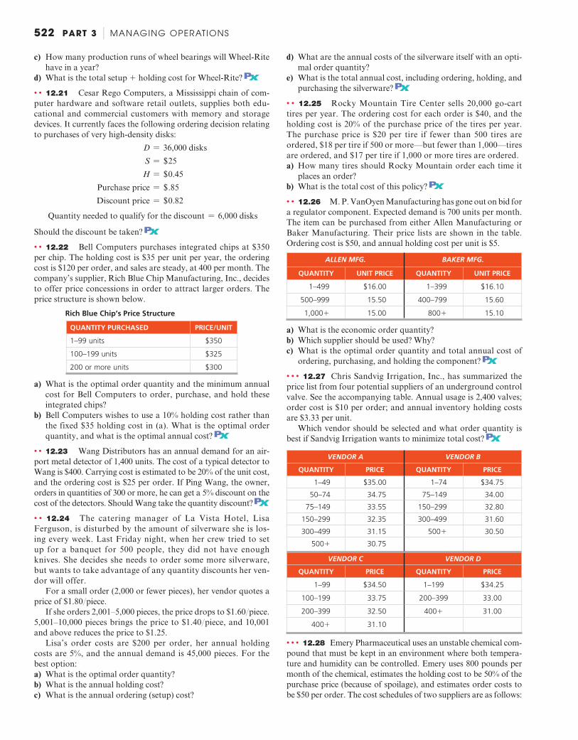
522 PART 3 | MANAGING OPERATIONS
c) How many production runs of wheel bearings will Wheel-Rite have in a year?
d) What is the total setup 1 holding cost for Wheel-Rite? PX
• • 12.21 Cesar Rego Computers, a Mississippi chain of com-puter hardware and software retail outlets, supplies both edu-cational and commercial customers with memory and storage devices. It currently faces the following ordering decision relating to purchases of very high-density disks:
D = 36,000 disks S = +25 H = +0.45 Purchase price = +.85 Discount price = +0.82
Quantity needed to qualify for the discount = 6,000 disks
Should the discount be taken? PX
• • 12.22 Bell Computers purchases integrated chips at $350 per chip. The holding cost is $35 per unit per year, the ordering cost is $120 per order, and sales are steady, at 400 per month. The company’s supplier, Rich Blue Chip Manufacturing, Inc., decides to offer price concessions in order to attract larger orders. The price structure is shown below.
Rich Blue Chip’s Price Structure
QUANTITY PURCHASED PRICE/UNIT
1–99 units $350
100–199 units $325
200 or more units $300
a) What is the optimal order quantity and the minimum annual cost for Bell Computers to order, purchase, and hold these integrated chips?
b) Bell Computers wishes to use a 10% holding cost rather than the fixed $35 holding cost in (a). What is the optimal order quantity, and what is the optimal annual cost? PX
• • 12.23 Wang Distributors has an annual demand for an air-port metal detector of 1,400 units. The cost of a typical detector to Wang is $400. Carrying cost is estimated to be 20% of the unit cost, and the ordering cost is $25 per order. If Ping Wang, the owner, orders in quantities of 300 or more, he can get a 5% discount on the cost of the detectors. Should Wang take the quantity discount? PX
• • 12.24 The catering manager of La Vista Hotel, Lisa Ferguson, is disturbed by the amount of silverware she is los-ing every week. Last Friday night, when her crew tried to set up for a banquet for 500 people, they did not have enough knives. She decides she needs to order some more silverware, but wants to take advantage of any quantity discounts her ven-dor will offer.
For a small order (2,000 or fewer pieces), her vendor quotes a price of $1.80Ypiece.
If she orders 2,001–5,000 pieces, the price drops to $1.60Ypiece. 5,001–10,000 pieces brings the price to $1.40Ypiece, and 10,001 and above reduces the price to $1.25.
Lisa’s order costs are $200 per order, her annual holding costs are 5%, and the annual demand is 45,000 pieces. For the best option: a) What is the optimal order quantity? b) What is the annual holding cost? c) What is the annual ordering (setup) cost?
d) What are the annual costs of the silverware itself with an opti-mal order quantity?
e) What is the total annual cost, including ordering, holding, and purchasing the silverware? PX
• • 12.25 Rocky Mountain Tire Center sells 20,000 go-cart tires per year. The ordering cost for each order is $40, and the holding cost is 20% of the purchase price of the tires per year. The purchase price is $20 per tire if fewer than 500 tires are ordered, $18 per tire if 500 or more—but fewer than 1,000—tires are ordered, and $17 per tire if 1,000 or more tires are ordered. a) How many tires should Rocky Mountain order each time it
places an order? b) What is the total cost of this policy? PX
• • 12.26 M. P. VanOyen Manufacturing has gone out on bid for a regulator component. Expected demand is 700 units per month. The item can be purchased from either Allen Manufacturing or Baker Manufacturing. Their price lists are shown in the table. Ordering cost is $50, and annual holding cost per unit is $5.
ALLEN MFG. BAKER MFG.
QUANTITY UNIT PRICE QUANTITY UNIT PRICE
1–499 $16.00 1–399 $16.10
500–999 15.50 400–799 15.60
1,0001 15.00 8001 15.10
a) What is the economic order quantity? b) Which supplier should be used? Why? c) What is the optimal order quantity and total annual cost of
ordering, purchasing, and holding the component? PX
• • • 12.27 Chris Sandvig Irrigation, Inc., has summarized the price list from four potential suppliers of an underground control valve. See the accompanying table. Annual usage is 2,400 valves; order cost is $10 per order; and annual inventory holding costs are $3.33 per unit.
Which vendor should be selected and what order quantity is best if Sandvig Irrigation wants to minimize total cost? PX
VENDOR A VENDOR B
QUANTITY PRICE QUANTITY PRICE
1–49 $35.00 1–74 $34.75
50–74 34.75 75–149 34.00
75–149 33.55 150–299 32.80
150–299 32.35 300–499 31.60
300–499 31.15 5001 30.50
5001 30.75
VENDOR C VENDOR D
QUANTITY PRICE QUANTITY PRICE
1–99 $34.50 1–199 $34.25
100–199 33.75 200–399 33.00
200–399 32.50 4001 31.00
4001 31.10
• • • 12.28 Emery Pharmaceutical uses an unstable chemical com-pound that must be kept in an environment where both tempera-ture and humidity can be controlled. Emery uses 800 pounds per month of the chemical, estimates the holding cost to be 50% of the purchase price (because of spoilage), and estimates order costs to be $50 per order. The cost schedules of two suppliers are as follows:
M16_HEIZ0422_12_SE_C12.indd 522M16_HEIZ0422_12_SE_C12.indd 522 05/11/15 5:04 PM05/11/15 5:04 PM
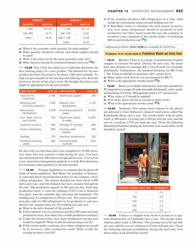
CHAPTER 12 | INVENTORY MANAGEMENT 523
VENDOR 1 VENDOR 2
QUANTITY PRICE/LB QUANTITY PRICE/LB
1–499 $17.00 1–399 $17.10
500–999 16.75 400–799 16.85
1,0001 16.50 800–1,199 16.60
1,2001 16.25
a) What is the economic order quantity for each supplier? b) What quantity should be ordered, and which supplier should
be used? c) What is the total cost for the most economic order size? d) What factor(s) should be considered besides total cost? PX
• • • 12.29 Kim Clark has asked you to help him determine the best ordering policy for a new product. The demand for the new product has been forecasted to be about 1,000 units annually. To help you get a handle on the carrying and ordering costs, Kim has given you the list of last year’s costs. He thought that these costs might be appropriate for the new product.
COST FACTOR COST ($) COST FACTOR COST ($)
Taxes for the warehouse
2,000 Warehouse supplies 280
Receiving and incoming inspection
1,500 Research and development
2,750
New product development
2,500 Purchasing salaries & wages
30,000
Acct. Dept. costs to pay invoices
500 Warehouse salaries & wages
12,800
Inventory insurance 600 Pilferage of inventory 800
Product advertising 800 Purchase order supplies
500
Spoilage 750 Inventory obsolescence 300
Sending purchasing orders
800 Purchasing Dept. overhead
1,000
He also told you that these data were compiled for 10,000 inven-tory items that were carried or held during the year. You have also determined that 200 orders were placed last year. Your job as a new operations management graduate is to help Kim determine the economic order quantity for the new product.
• • • • 12.30 Emarpy Appliance is a company that produces all kinds of major appliances. Bud Banis, the president of Emarpy, is concerned about the production policy for the company’s best-selling refrigerator. The annual demand has been about 8,000 units each year, and this demand has been constant throughout the year. The production capacity is 200 units per day. Each time production starts, it costs the company $120 to move materials into place, reset the assembly line, and clean the equipment. The holding cost of a refrigerator is $50 per year. The current produc-tion plan calls for 400 refrigerators to be produced in each pro-duction run. Assume there are 250 working days per year. a) What is the daily demand of this product? b) If the company were to continue to produce 400 units each time
production starts, how many days would production continue? c) Under the current policy, how many production runs per year
would be required? What would the annual setup cost be? d) If the current policy continues, how many refrigerators would
be in inventory when production stops? What would the average inventory level be?
e) If the company produces 400 refrigerators at a time, what would the total annual setup cost and holding cost be?
f ) If Bud Banis wants to minimize the total annual inventory cost, how many refrigerators should be produced in each production run? How much would this save the company in inventory costs compared to the current policy of producing 400 in each production run? PX
Additional problems 12.31–12.40 are available in MyOMLab.
Problems 12.41–12.50 relate to Probabilistic Models and Safety Stock
• • 12.41 Barbara Flynn is in charge of maintaining hospital supplies at General Hospital. During the past year, the mean lead time demand for bandage BX-5 was 60 (and was normally distributed). Furthermore, the standard deviation for BX-5 was 7. Ms. Flynn would like to maintain a 90% service level. a) What safety stock level do you recommend for BX-5? b) What is the appropriate reorder point? PX
• • 12.42 Based on available information, lead time demand for PC jump drives averages 50 units (normally distributed), with a stand-ard deviation of 5 drives. Management wants a 97% service level. a) What value of Z should be applied? b) How many drives should be carried as safety stock? c) What is the appropriate reorder point? PX
••• 12.43 Authentic Thai rattan chairs (shown in the photo) are delivered to Gary Schwartz’s chain of retail stores, called The Kathmandu Shop, once a year. The reorder point, without safety stock, is 200 chairs. Carrying cost is $30 per unit per year, and the cost of a stockout is $70 per chair per year. Given the following demand probabilities during the lead time, how much safety stock should be carried?
Bar
ry R
ende
r
DEMAND DURING LEAD TIME PROBABILITY
0 0.2
100 0.2
200 0.2
300 0.2
400 0.2
• • 12.44 Tobacco is shipped from North Carolina to a ciga-rette manufacturer in Cambodia once a year. The reorder point, without safety stock, is 200 kilos. The carrying cost is $15 per kilo per year, and the cost of a stockout is $70 per kilo per year. Given the following demand probabilities during the lead time, how much safety stock should be carried?
M16_HEIZ0422_12_SE_C12.indd 523M16_HEIZ0422_12_SE_C12.indd 523 05/11/15 5:04 PM05/11/15 5:04 PM
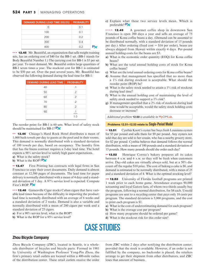
524 PART 3 | MANAGING OPERATIONS
c) Explain what these two service levels mean. Which is preferable? PX
• • • • 12.49 A gourmet coffee shop in downtown San Francisco is open 200 days a year and sells an average of 75 pounds of Kona coffee beans a day. (Demand can be assumed to be distributed normally, with a standard deviation of 15 pounds per day.) After ordering (fixed cost 5 $16 per order), beans are always shipped from Hawaii within exactly 4 days. Per-pound annual holding costs for the beans are $3. a) What is the economic order quantity (EOQ) for Kona coffee
beans? b) What are the total annual holding costs of stock for Kona
coffee beans? c) What are the total annual ordering costs for Kona coffee beans? d) Assume that management has specified that no more than
a 1% risk during stockout is acceptable. What should the reorder point (ROP) be?
e) What is the safety stock needed to attain a 1% risk of stockout during lead time?
f ) What is the annual holding cost of maintaining the level of safety stock needed to support a 1% risk?
g) If management specified that a 2% risk of stockout during lead time would be acceptable, would the safety stock holding costs decrease or increase?
Additional problem 12.50 is available in MyOMLab.
Problems 12.51–12.53 relate to Single-Period Model
•• 12.51 Cynthia Knott’s oyster bar buys fresh Louisiana oysters for $5 per pound and sells them for $9 per pound. Any oysters not sold that day are sold to her cousin, who has a nearby grocery store, for $2 per pound. Cynthia believes that demand follows the normal distribution, with a mean of 100 pounds and a standard deviation of 15 pounds. How many pounds should she order each day?
•• 12.52 Henrique Correa’s bakery prepares all its cakes between 4 a.m. and 6 a.m. so they will be fresh when customers arrive. Day-old cakes are virtually always sold, but at a 50% dis-count off the regular $10 price. The cost of baking a cake is $6, and demand is estimated to be normally distributed, with a mean of 25 and a standard deviation of 4. What is the optimal stocking level?
••• 12.53 University of Florida football programs are printed 1 week prior to each home game. Attendance averages 90,000 screaming and loyal Gators fans, of whom two-thirds usually buy the program, following a normal distribution, for $4 each. Unsold programs are sent to a recycling center that pays only 10 cents per program. The standard deviation is 5,000 programs, and the cost to print each program is $1. a) What is the cost of underestimating demand for each program? b) What is the overage cost per program? c) How many programs should be ordered per game? d) What is the stockout risk for this order size?
CASE STUDIES Zhou Bicycle Company
Zhou Bicycle Company (ZBC), located in Seattle, is a whole-sale distributor of bicycles and bicycle parts. Formed in 1981 by University of Washington Professor Yong-Pin Zhou, the firm’s primary retail outlets are located within a 400-mile radius of the distribution center. These retail outlets receive the order
from ZBC within 2 days after notifying the distribution center, provided that the stock is available. However, if an order is not fulfilled by the company, no backorder is placed; the retailers arrange to get their shipment from other distributors, and ZBC loses that amount of business.
DEMAND DURING LEAD TIME (KILOS) PROBABILITY
0 0.1
100 0.1
200 0.2
300 0.4
400 0.2
• • • 12.45 Mr. Beautiful, an organization that sells weight training sets, has an ordering cost of $40 for the BB-1 set. (BB-1 stands for Body Beautiful Number 1.) The carrying cost for BB-1 is $5 per set per year. To meet demand, Mr. Beautiful orders large quantities of BB-1 seven times a year. The stockout cost for BB-1 is estimated to be $50 per set. Over the past several years, Mr. Beautiful has observed the following demand during the lead time for BB-1:
DEMAND DURING LEAD TIME PROBABILITY
40 .1
50 .2
60 .2
70 .2
80 .2
90 .1
1.0
The reorder point for BB-1 is 60 sets. What level of safety stock should be maintained for BB-1? PX
• • 12.46 Chicago’s Hard Rock Hotel distributes a mean of 1,000 bath towels per day to guests at the pool and in their rooms. This demand is normally distributed with a standard deviation of 100 towels per day, based on occupancy. The laundry firm that has the linens contract requires a 2-day lead time. The hotel expects a 98% service level to satisfy high guest expectations. a) What is the safety stock? b) What is the ROP? PX
•• 12.47 First Printing has contracts with legal firms in San Francisco to copy their court documents. Daily demand is almost constant at 12,500 pages of documents. The lead time for paper delivery is normally distributed with a mean of 4 days and a stand-ard deviation of 1 day. A 97% service level is expected. Compute First’s ROP. PX
• • • 12.48 Gainesville Cigar stocks Cuban cigars that have vari-able lead times because of the difficulty in importing the product: lead time is normally distributed with an average of 6 weeks and a standard deviation of 2 weeks. Demand is also a variable and normally distributed with a mean of 200 cigars per week and a standard deviation of 25 cigars. a) For a 90% service level, what is the ROP? b) What is the ROP for a 95% service level?
PX
M16_HEIZ0422_12_SE_C12.indd 524M16_HEIZ0422_12_SE_C12.indd 524 05/11/15 5:04 PM05/11/15 5:04 PM

CHAPTER 12 | INVENTORY MANAGEMENT 525
Parker Hi-Fi Systems
Parker Hi-Fi Systems, located in Wellesley, Massachusetts, a Boston suburb, assembles and sells the very finest home theater sys-tems. The systems are assembled with components from the best manufacturers worldwide. Although most of the components are procured from wholesalers on the East Coast, some critical items, such as LCD screens, come directly from their manufacturer. For instance, the LCD screens are shipped via air from Foxy, Ltd., in Taiwan, to Boston’s Logan airport, and the top-of-the-line speakers are purchased from the world-renowned U.S. manufacturer Boss.
Parker’s purchasing agent, Raktim Pal, submits an order release for LCD screens once every 4 weeks. The company’s annual requirements total 500 units (2 per working day), and Parker’s per unit cost is $1,500. (Because of Parker’s relatively low volume and the quality focus—rather than volume focus—of many of Parker’s suppliers, Parker is seldom able to obtain quantity discounts.) Because Foxy promises delivery within 1 week following receipt of an order release, Parker has never had a shortage of LCDs. (Total time between date of the release and date of receipt is 1 week or 5 working days.)
Parker’s activity-based costing system has generated the fol-lowing inventory-related costs. Procurement costs, which amount to $500 per order, include the actual labor costs involved in order-ing, customs inspection, arranging for airport pickup, delivery to the plant, maintaining inventory records, and arranging for the bank to issue a check. Parker’s holding costs take into account storage, damage, insurance, taxes, and so forth on a square-foot basis. These costs equal $150 per LCD per year.
With added emphasis being placed on efficiencies in the supply chain, Parker’s president has asked Raktim to seriously evaluate the purchase of the LCDs. One area to be closely scrutinized for possible cost savings is inventory procurement.
Discussion Questions
1. What is the optimal order number of LCDs that should be placed in each order?
2. What is the optimal reorder point (ROP) for LCDs? 3. What cost savings will Parker realize if it implements an order
plan based on EOQ?
The company distributes a wide variety of bicycles. The most popular model, and the major source of revenue to the company, is the AirWing. ZBC receives all the models from a single manufacturer in China, and shipment takes as long as 4 weeks from the time an order is placed. With the cost of com-munication, paperwork, and customs clearance included, ZBC estimates that each time an order is placed, it incurs a cost of $65. The purchase price paid by ZBC, per bicycle, is roughly 60% of the suggested retail price for all the styles available, and the inventory carrying cost is 1% per month (12% per year) of the purchase price paid by ZBC. The retail price (paid by the customers) for the AirWing is $170 per bicycle.
ZBC is interested in making an inventory plan for 2016. The firm wants to maintain a 95% service level with its customers to minimize the losses on the lost orders. The data collected for the past 2 years are summarized in the following table. A forecast for AirWing model sales in 2016 has been developed and will be used to make an inventory plan for ZBC.
Demands For Airwing Model
MONTH 2014 2015 FORECAST FOR 2016
January 6 7 8February 12 14 15
MONTH 2014 2015 FORECAST FOR 2016
March 24 27 31April 46 53 59May 75 86 97June 47 54 60July 30 34 39August 18 21 24September 13 15 16October 12 13 15November 22 25 28December 38 42 47 Total 343 391 439
Discussion Questions
1. Develop an inventory plan to help ZBC. 2. Discuss ROPs and total costs. 3. How can you address demand that is not at the level of the
planning horizon?
Source: Professor Kala Chand Seal, Loyola Marymount University.
Managing Inventory at Frito-Lay Video Case Frito-Lay has flourished since its origin—the 1931 purchase of a small San Antonio firm for $100 that included a recipe, 19 retail accounts, and a hand-operated potato ricer. The multi-billion- dollar company, headquartered in Dallas, now has 41 products—15 with sales of over $100 million per year and 7 at over $1 billion in sales. Production takes place in 36 product-focused plants in the U.S. and Canada, with 48,000 employees.
Inventory is a major investment and an expensive asset in most firms. Holding costs often exceed 25% of product value, but in Frito-Lay’s prepared food industry, holding cost can be much higher because the raw materials are perishable. In the food industry, inventory spoils. So poor inventory management is not only expensive but can also yield an unsatisfactory product that in the extreme can also ruin market acceptance.
Major ingredients at Frito-Lay are corn meal, corn, potatoes, oil, and seasoning. Using potato chips to illustrate rapid inventory
flow: potatoes are moved via truck from farm, to regional plants for processing, to warehouse, to the retail store. This happens in a matter of hours—not days or weeks. This keeps freshness high and holding costs low.
Frequent deliveries of the main ingredients at the Florida plant, for example, take several forms:
◆ Potatoes are delivered in 10 truckloads per day, with 150,000 lbs consumed in one shift: the entire potato storage area will only hold 7½ hours’ worth of potatoes.
◆ Oil inventory arrives by rail car, which lasts only 4½ days. ◆ Corn meal arrives from various farms in the Midwest, and
inventory typically averages 4 days’ production. ◆ Seasoning inventory averages 7 days. ◆ Packaging inventory averages 8 to 10 days.
M16_HEIZ0422_12_SE_C12.indd 525M16_HEIZ0422_12_SE_C12.indd 525 05/11/15 5:04 PM05/11/15 5:04 PM

526 PART 3 | MANAGING OPERATIONS
Inventory Control at Wheeled Coach
Controlling inventory is one of Wheeled Coach’s toughest prob-lems. Operating according to a strategy of mass customization and responsiveness, management knows that success is depend-ent on tight inventory control. Anything else results in an inabil-ity to deliver promptly, chaos on the assembly line, and a huge inventory investment. Wheeled Coach finds that almost 50% of the cost of every ambulance it manufactures is purchased materi-als. A large proportion of that 50% is in chassis (purchased from Ford), aluminum (from Reynolds Metal), and plywood used for flooring and cabinetry construction (from local suppliers). Wheeled Coach tracks these A inventory items quite carefully, maintaining tight security/control and ordering carefully so as to maximize quantity discounts while minimizing on-hand stock. Because of long lead times and scheduling needs at Reynolds, aluminum must actually be ordered as much as 8 months in advance.
In a crowded ambulance industry in which it is the only giant, its 45 competitors don’t have the purchasing power to draw the same discounts as Wheeled Coach. But this competitive cost advantage cannot be taken lightly, according to President Bob Collins. “Cycle
counting in our stockrooms is critical. No part can leave the locked stockrooms without appearing on a bill of materials.”
Accurate bills of material (BOM) are a requirement if prod-ucts are going to be built on time. Additionally, because of the custom nature of each vehicle, most orders are won only after a bidding process. Accurate BOMs are critical to cost estimation and the resulting bid. For these reasons, Collins was emphatic that Wheeled Coach maintain outstanding inventory control. The Global Company Profile featuring Wheeled Coach (which opens Chapter 14 ) provides further details about the ambulance inven-tory control and production process.
Discussion Questions *
1. Explain how Wheeled Coach implements ABC analysis. 2. If you were to take over as inventory control manager at
Wheeled Coach, what additional policies and techniques would you initiate to ensure accurate inventory records?
3. How would you go about implementing these suggestions?
* You may wish to view the video that accompanies this case before addressing these questions.
* You may wish to view the video that accompanies this case before addressing these questions.
• Additional Case Studies: Visit MyOMLab for these free case studies: Southwestern University (F): The university must decide how many football day programs to order, and from whom. LaPlace Power and Light: This utility company is evaluating its current inventory policies.
Endnotes
1. See E. Malykhina, “Retailers Take Stock,” Information Week (February 7, 2005): 20–22, and A. Raman, N. DeHoratius, and Z. Ton, “Execution: The Missing Link in Retail Operations,” California Management Review 43, no. 3 (Spring 2001): 136–141.
2. This is the case when holding costs are linear and begin at the origin—that is, when inventory costs do not decline (or they increase) as inventory volume increases and all holding costs are in small increments. In addition, there is probably some learning each time a setup (or order) is executed—a fact that lowers subsequent setup costs. Consequently, the EOQ model is probably a special case. However, we abide by the conven-tional wisdom that this model is a reasonable approximation.
3. The formula for the economic order quantity ( Q *) can also be determined by finding where the total cost curve is at a minimum (i.e., where the slope of the total cost curve is zero). Using calculus, we set the derivative of the total cost with respect to Q * equal to 0.
The calculations for finding the minimum of
TC =DQ
S +Q2
H + PD
are d(TC)
dQ= ¢ 9DS
Q2 ≤ +H2
+ 0 = 0
Thus, Q* =A
2DSH
4. The number of units short, Demand–ROP, is true only when Demand–ROP is non-negative.
5. Equations (12-15), (12-16), and (12-17) are expressed in days; however, they could equivalently be expressed in weeks, months, or even years. Just be consistent, and use the same time units for all terms in the equations.
6. Note that Equation (12-17) can also be expressed as: ROP = Average daily demand * Average lead time +
Z2(Average lead time * sd 2) + d 2
sLT 2 .
7. OM managers also call these continuous review systems .
Frito-Lay’s product-focused facility represents a major capital investment. That investment must achieve high utilization to be efficient. The capital cost must be spread over a substantial volume to drive down total cost of the snack foods produced. This demand for high utilization requires reliable equipment and tight schedules. Reliable machinery requires an inventory of critical components: this is known as MRO, or maintenance, repair, and operating sup-plies. MRO inventory of motors, switches, gears, bearings, and other critical specialized components can be costly but is necessary.
Frito-Lay’s non-MRO inventory moves rapidly. Raw mate-rial quickly becomes work-in-process, moving through the system and out the door as a bag of chips in about 11
2 shifts. Packaged finished products move from production to the distribution chain in less than 1.4 days.
Discussion Questions *
1. How does the mix of Frito-Lay’s inventory differ from those at a machine or cabinet shop (a process-focused facility)?
2. What are the major inventory items at Frito-Lay, and how rapidly do they move through the process?
3. What are the four types of inventory? Give an example of each at Frito-Lay.
4. How would you rank the dollar investment in each of the four types (from the most investment to the least investment)?
5. Why does inventory flow so quickly through a Frito-Lay plant? 6. Why does the company keep so many plants open? 7. Why doesn’t Frito-Lay make all its 41 products at each of its plants?
Video Case
M16_HEIZ0422_12_SE_C12.indd 526M16_HEIZ0422_12_SE_C12.indd 526 05/11/15 5:04 PM05/11/15 5:04 PM

Rapi
d Re
view
12 Chapter 12 Rapid Review Main Heading Review Material MyOMLab THE IMPORTANCE OF INVENTORY (pp. 490–491)
Inventory is one of the most expensive assets of many companies. The objective of inventory management is to strike a balance between inventory investment and customer service. The two basic inventory issues are how much to order and when to order. j Raw material inventory —Materials that are usually purchased but have yet to
enter the manufacturing process. j Work-in-process (WIP) inventory —Products or components that are no longer
raw materials but have yet to become finished products. j MRO inventory —Maintenance, repair, and operating materials. j Finished-goods inventory —An end item ready to be sold but still an asset on the
company’s books.
Concept Questions: 1.1–1.4 VIDEO 12.1 Managing Inventory at Frito-Lay
MANAGING INVENTORY (pp. 491–495)
j ABC analysis —A method for dividing on-hand inventory into three classifications based on annual dollar volume.
j Cycle counting —A continuing reconciliation of inventory with inventory records. j Shrinkage —Retail inventory that is unaccounted for between receipt and sale. j Pilferage —A small amount of theft.
Concept Questions: 2.1–2.4 Problems: 12.1–12.6 Virtual Office Hours for Solved Problem: 12.1
INVENTORY MODELS (pp. 495–496)
j Holding cost —The cost to keep or carry inventory in stock. j Ordering cost —The cost of the ordering process. j Setup cost —The cost to prepare a machine or process for production. j Setup time —The time required to prepare a machine or process for production.
Concept Questions: 3.1–3.4 VIDEO 12.2 Inventory Control at Wheeled Coach Ambulance
INVENTORY MODELS FOR INDEPENDENT DEMAND (pp. 496–507)
j Economic order quantity (EOQ) model —An inventory-control technique that minimizes the total of ordering and holding costs:
Q* =A
2DSH
(12-1)
Expected number of orders = N =Demand
Order quantity=
DQ*
(12-2)
Expected time between orders = T =Number of working days per year
N (12-3)
Total annual cost = Setup (order) cost + Holding cost (12-4)
TC =DQ
S +Q2
H (12-5)
j Robust —Giving satisfactory answers even with substantial variation in the parameters.
j Lead time —In purchasing systems, the time between placing an order and receiv-ing it; in production systems, the wait, move, queue, setup, and run times for each component produced.
j Reorder point (ROP) —The inventory level (point) at which action is taken to replenish the stocked item.
ROP for known demand: ROP = Demand per day * Lead time for a new order in days = d * L (12-6) j Safety stock ( ss ) —Extra stock to allow for uneven demand; a buffer. j Production order quantity model —An economic order quantity technique applied
to production orders:
Q*p =A
2DSH31 - (d>p)4
(12-7)
Q*p =
H
2DS
Ha1 -Annual demand rate
Annual production rateb
(12-8)
j Quantity discount —A reduced price for items purchased in large quantities:
TC =DQ
S +Q2
H + PD (12-9)
Q* =A
2DSIP
(12-10)
Concept Questions: 4.1–4.4 Problems: 12.7–12.40 Virtual Office Hours for Solved Problems: 12.2–12.5 ACTIVE MODELS 12.1, 12.2
M16_HEIZ0422_12_SE_C12.indd 527M16_HEIZ0422_12_SE_C12.indd 527 05/11/15 5:04 PM05/11/15 5:04 PM

Rapi
d Re
view
12 Chapter 12 Rapid Review continued
Main Heading Review Material MyOMLab PROBABILISTIC MODELS AND SAFETY STOCK (pp. 508–513)
j Probabilistic model —A statistical model applicable when product demand or any other variable is not known but can be specified by means of a probability distribution.
j Service level —The complement of the probability of a stockout. ROP for unknown demand: ROP = d * L + ss (12-11)
Annual stockout costs = The sum of the units short for each demand level
* The probability of that demand level * The stockout cost>unit* The number of orders per year
(12-12)
ROP for unknown demand and given service level: ROP = Expected demand during lead time + ZsdLT (12-13) Safety stock = ZsdLT (12-14) ROP for variable demand and constant lead time: ROP = (Average daily demand * Lead time in days) + ZsdLT (12-15) ROP for constant demand and variable lead time: ROP = (Daily demand * Average lead time in days) + Z * Daily demand * sLT
(12-16) ROP for variable demand and variable lead time: ROP = (Average daily demand * Average lead time in days) + ZsdLT (12-17) In each case, sdLT = 2(Average lead time * sd
2) + d2s2LT
but under constant demand: s2d = 0,
and under constant lead time: s2LT = 0.
Concept Questions: 5.1–5.4 Problems: 12.41–12.50 Virtual Office Hours for Solved Problems: 12.6–12.9
SINGLE-PERIOD MODEL (pp. 513–514 )
j Single-period inventory model —A system for ordering items that have little or no value at the end of the sales period:
Service level =Cs
Cs + Co (12-18)
Concept Questions: 6.1–6.4 Problems: 12.51–12.53
FIXED-PERIOD ( P ) SYSTEMS (pp. 514–515)
j Fixed-quantity ( Q ) system —An ordering system with the same order amount each time. j Perpetual inventory system —A system that keeps track of each withdrawal or
addition to inventory continuously, so records are always current. j Fixed-period ( P ) system —A system in which inventory orders are made at regular
time intervals.
Concept Questions: 7.1–7.4
Self Test
LO 12.1 ABC analysis divides on-hand inventory into three classes, based on:
a) unit price. b) the number of units on hand. c) annual demand. d) annual dollar values. LO 12.2 Cycle counting: a) provides a measure of inventory turnover. b) assumes that all inventory records must be verified with
the same frequency. c) is a process by which inventory records are periodically
verified. d) all of the above. LO 12.3 The two most important inventory-based questions
answered by the typical inventory model are: a) when to place an order and the cost of the order. b) when to place an order and how much of an item
to order. c) how much of an item to order and the cost of the order. d) how much of an item to order and with whom the order
should be placed. LO 12.4 Extra units in inventory to help reduce stockouts are called: a) reorder point. b) safety stock. c) just-in-time inventory. d) all of the above.
LO 12.5 The difference(s) between the basic EOQ model and the pro-duction order quantity model is(are) that:
a) the production order quantity model does not require the assumption of known, constant demand.
b) the EOQ model does not require the assumption of negligible lead time.
c) the production order quantity model does not require the assumption of instantaneous delivery.
d) all of the above. LO 12.6 The EOQ model with quantity discounts attempts to
determine: a) the lowest amount of inventory necessary to satisfy a
certain service level. b) the lowest purchase price. c) whether to use a fixed-quantity or fixed-period order policy. d) how many units should be ordered. e) the shortest lead time. LO 12.7 The appropriate level of safety stock is typically determined by: a) minimizing an expected stockout cost. b) choosing the level of safety stock that assures a given
service level. c) carrying sufficient safety stock so as to eliminate all stockouts. d) annual demand.
Answers: LO 12.1. d; LO 12.2. c; LO 12.3. b; LO 12.4. b; LO 12.5. c; LO 12.6. d; LO 12.7. b.
j Before taking the self-test, refer to the learning objectives listed at the beginning of the chapter and the key terms listed at the end of the chapter.
M16_HEIZ0422_12_SE_C12.indd 528M16_HEIZ0422_12_SE_C12.indd 528 05/11/15 5:04 PM05/11/15 5:04 PM