Hein, Schierup & Wiuf: Genealogies, Variation & Evolution. ([email protected]).
44
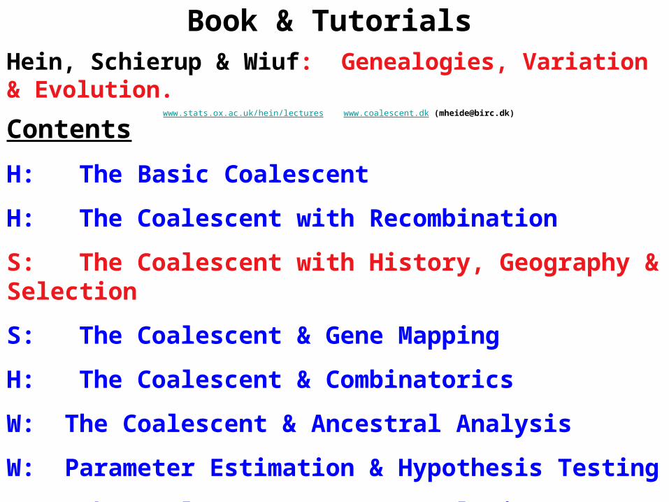
Hein, Schierup & Wiuf: Genealogies, Variation & Evolution. www.stats.ox.ac.uk/hein/lectures www.coalescent.dk ([email protected]) Contents H: The Basic Coalescent H: The Coalescent with Recombination S: The Coalescent with History, Geography & Selection S: The Coalescent & Gene Mapping H: The Coalescent & Combinatorics W: The Coalescent & Ancestral Analysis W: Parameter Estimation & Hypothesis Testing H: The Coalescent & Human Evolution Book & Tutorials
-
date post
19-Dec-2015 -
Category
Documents
-
view
220 -
download
1
Transcript of Hein, Schierup & Wiuf: Genealogies, Variation & Evolution. ([email protected]).
Hein, Schierup & Wiuf: Genealogies, Variation & Evolution.www.stats.ox.ac.uk/hein/lectures www.coalescent.dk ([email protected])
Contents
H: The Basic Coalescent
H: The Coalescent with Recombination
S: The Coalescent with History, Geography & Selection
S: The Coalescent & Gene Mapping
H: The Coalescent & Combinatorics
W: The Coalescent & Ancestral Analysis
W: Parameter Estimation & Hypothesis Testing
H: The Coalescent & Human Evolution
Book & Tutorials
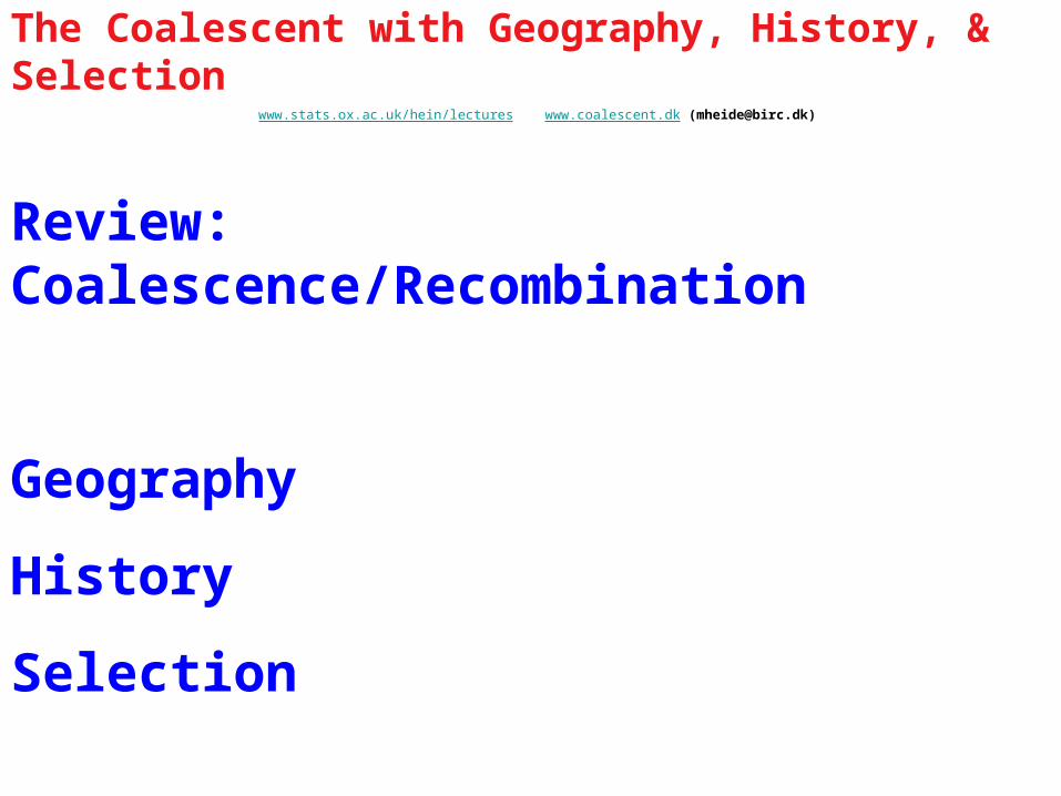
The Coalescent with Geography, History, & Selectionwww.stats.ox.ac.uk/hein/lectures www.coalescent.dk ([email protected])
Review: Coalescence/Recombination
Geography
History
Selection
Scenarios Detection

Continuous-Time Coalescent
1 24 56 3 0.0
1.0
1.0 corresponds to 2N generations
0
2N
Discrete Continuous

Recombination-Coalescence IllustrationCopied from Hudson 1990 Intensities
Coales. Recomb.
1 2
3 2
6 2
3 (2+b)
1 (1+b)
0
b
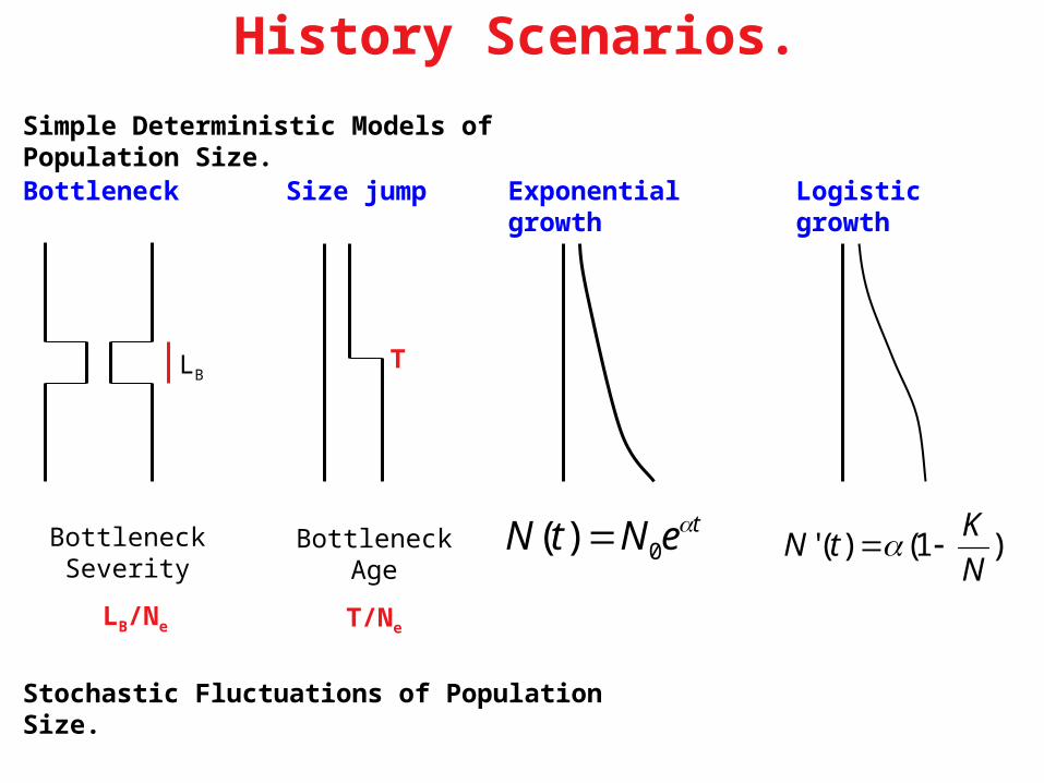
History Scenarios.
Logistic growthBottleneck Size jump Exponential growth
Stochastic Fluctuations of Population Size.
Simple Deterministic Models of Population Size.
LB
Bottleneck Severity
LB/Ne
Bottleneck Age
T/Ne
teNtN 0)( )1()('
N
KtN
T
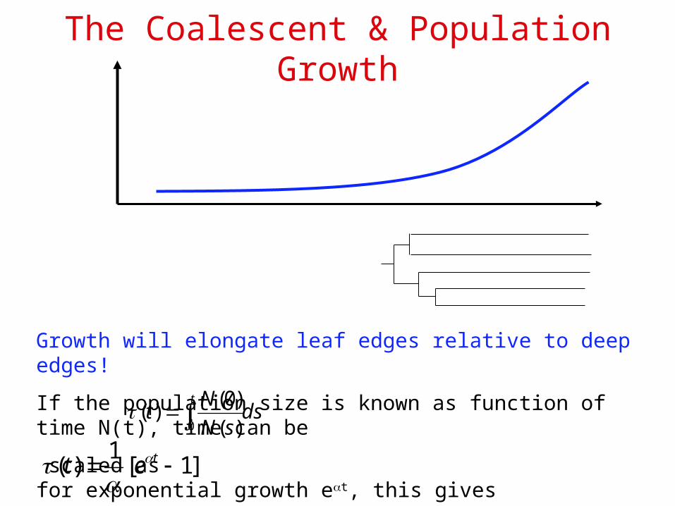
The Coalescent & Population Growth
Growth will elongate leaf edges relative to deep edges!
If the population size is known as function of time N(t), time can be
scaled as for exponential growth et, this givesdssN
Nt
t
0 )(
)0()(
]1[1
)( tet

Tests of History.
Distortion of branch lengths towards the present.
Tajima (1989) - Fu and Li (1993)
Mismatch Distribution Pairwise Distances
Rogers & Harpending,1992.
Likelihood Models
Beerli & Felsenstein,1999
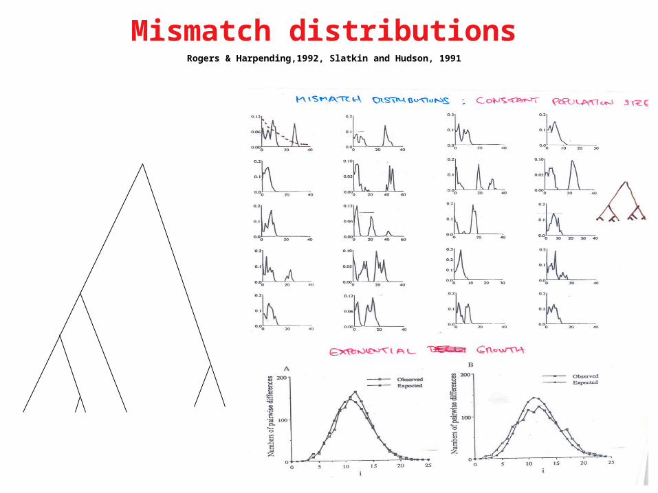
Mismatch distributionsRogers & Harpending,1992, Slatkin and Hudson, 1991
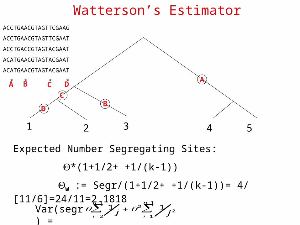
Watterson’s Estimator
1 2 3 54
ACCTGAACGTAGTTCGAAG
ACCTGAACGTAGTTCGAAT
ACCTGACCGTAGTACGAAT
ACATGAACGTAGTACGAAT
ACATGAACGTAGTACGAAT
* * * *
Expected Number Segregating Sites:
*(1+1/2+ +1/(k-1))
W := Segr/(1+1/2+ +1/(k-1))= 4/ [11/6]=24/11=2.1818
Var(segr) =
1j
i2
n1
2 1j2
i1
n1
AA
B
B C
C
D
D

Pairwise Distance Estimator
1 2 3 54
PD := Average Pairwise Distance (above 2.166)
VarPD) = (n+1)/3(n-1) + 2 2(n2+n+3)/9n(n-1)
44
4 44
6
6
A mutation on a (n,n-k) branch will be counted n*(n-k) times. I.e. deep branches have higher weights.
A
ACCTGAACGTAGTTCGAAG
ACCTGAACGTAGTTCGAAT
ACCTGACCGTAGTACGAAT
ACATGAACGTAGTACGAAT
ACATGAACGTAGTACGAAT
* * * *
BC
D
A B C D

D = (PD -W)/Sd(PD -W)
A large value indicates shortened tips
A small value indicates shortened deep branches.
Tajima’s Test
Mitochondria (Ingman et al. 2000) Remade from McVean
52 complete molecules
521 segregating sites
PD = 44.2 W = 115.3
V(D) =31.8 D = -2.23
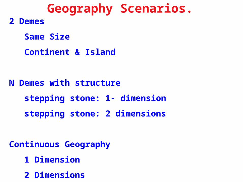
Geography Scenarios.2 Demes
Same Size
Continent & Island
N Demes with structure
stepping stone: 1- dimension
stepping stone: 2 dimensions
Continuous Geography
1 Dimension
2 Dimensions

Two Demes:
Symmetric:
Island/Continent:
M1
M2
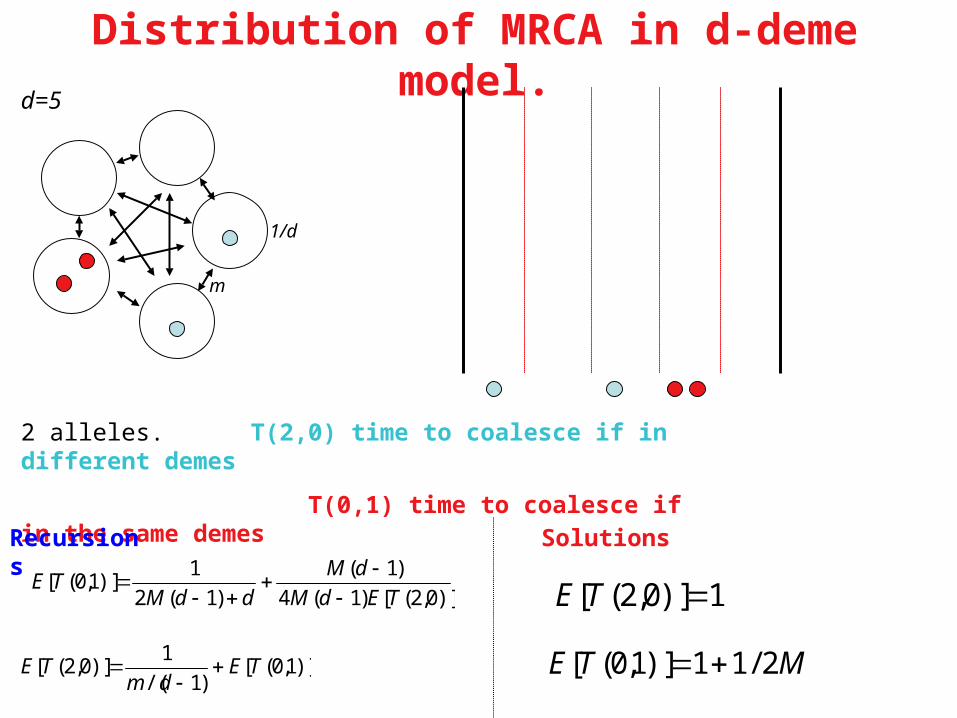
Distribution of MRCA in d-deme model.
2 alleles. T(2,0) time to coalesce if in different demes
T(0,1) time to coalesce if in the same demes
Recursions Solutions
)]0,2([)1(4
)1(
)1(2
1)]1,0([
TEdM
dM
ddMTE
)]1,0([)1/(
1)]0,2([ TE
dmTE
MTE 2/11)]1,0([
1)]0,2([ TE
d=5
m
1/d
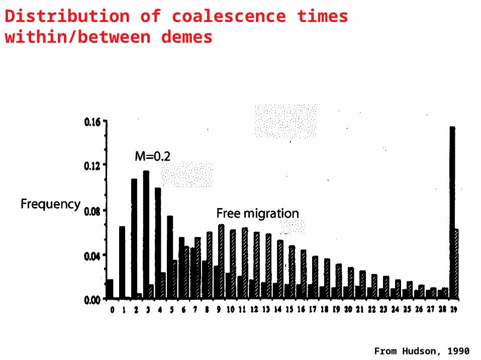
From Hudson, 1990
Distribution of coalescence times within/between demes

Population subdivision - two demes
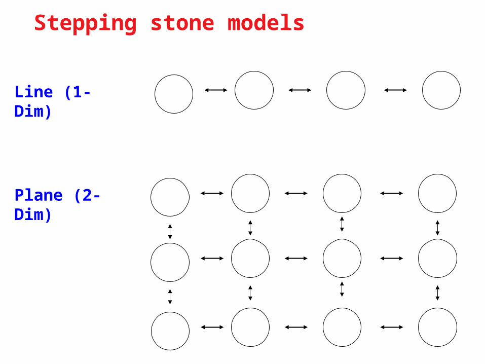
Stepping stone models
Line (1-Dim)
Plane (2-Dim)
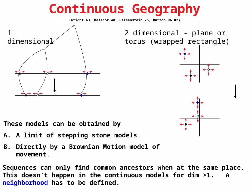
Continuous Geography(Wright 43, Malecot 48, Felsenstein 75, Barton 96 02)
1 dimensional 2 dimensional - plane or torus (wrapped rectangle)
These models can be obtained by
A. A limit of stepping stone models
B. Directly by a Brownian Motion model of movement.
Sequences can only find common ancestors when at the same place. This doesn’t happen in the continuous models for dim >1. A neighborhood has to be defined.
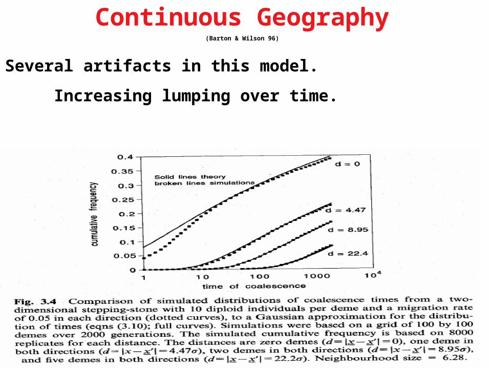
Continuous Geography(Barton & Wilson 96)
Several artifacts in this model.
Increasing lumping over time.

Testing Geography.
Hudson, Boos & Slatkin’s (1990) Permutation test
Maddison & Slatkin (1989) Assignment of ancestral geography.
Likelihood Bahlo & Griffiths (2000) Pritchard’s Structure (2000) Kuhner et al. (2000)

Selection Scenarios.
Haploid
Selection Directional
Frequency Dependent
Diploid
Balancing Selection
Directional Selection
Allelic Types
Alleles: A a
Fitnesses 1 1-s
Fitnesses 1-pA 1-pa
Genotypes AA AA aa
Fitnesses 1 1+s 1
Fitnesses 1 1+hs 1+s
sNs In the coalescent scaling

The 1983 Kreitman Data(M. Kreitman 1983 Nature) from Hartl & Clark, 1997
11 alleles 3200 bp long.
43 segregating sites (columns with variation).
1 amino replacement event
1 insertion-deletion (indel)

P(A)=p, P(B)=q, we sample k1 A alleles and k2 B alleles
Two locus balancing selection modelHudson, Darden & Kaplan,88-89
q p
Two cases:
Strong selection with fixed ancestral frequencies
Weaker selection with fluctuating ancestral frequencies.
k1 k2

Directional Selection/ Bottlenecks

Geography Selection
Local Global
Heterogenisation Balancing Selection Geo.Subdivision
Homogenisation Selective Sweeps Bottlenecks

Two alleles, A and a, A has an advantage of sMutation rate between types = u
The ancestral selection graphKrone & Neuhauser, 1997
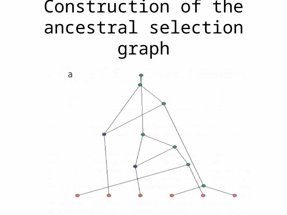
Construction of the ancestral selection graph
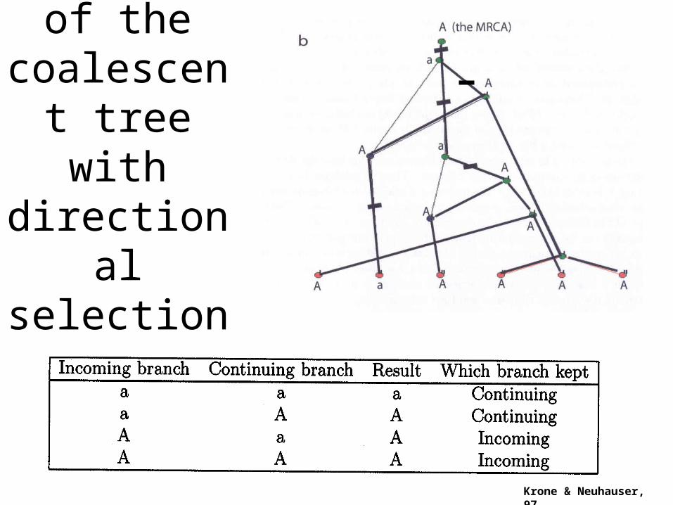
Recovery of the
coalescent tree with
directional selection
Krone & Neuhauser, 97

A Coalescent relating Allele Classes.(Takahata,1990)
AiAj AiAi
1 1-s
2
3
2)
16ln(
2
M
S
M
sfS
NM NsS
Examples: Major Histocompatibility Genes
Self-incompatibility Alleles in plants.
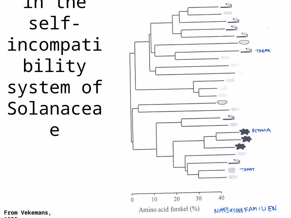
Allelic genealogy in
the self-incompatibility system of Solanaceae
From Vekemans, 1998

Tests of Selection
Tajima’s D (1989) (Fu’s test)
Hudson, Kreitman & Aquade (1987) HKA
Kreitman-MacDonald test (1990)
Likelihood tests

HKA-Test (Hudson, Kreitman & Aquade)Hudson,Kreitman & Aquade,1987
Gene 1
Specie 1 Specie 2
1
Speciation, T:
MRCA1
Gene 2
Specie 1 Specie 2
2
Speciation, T:
MRCA2
Are the 2 loci linked or unlinked?
The original data set ADH & 5’ prime region, D. sechellia & D.melanogaster
d=210 (MRCA1) d=18 (MRCA2)
S=9 (Lk1*1) S=8 (Lk2*2)
1 = 2.7 2=0.7 T=13.4Ne
Rejection.
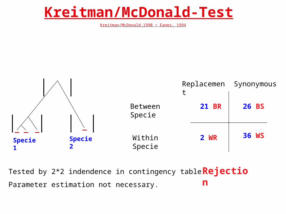
Kreitman/McDonald-Test Kreitman/McDonald,1990 + Eanes, 1994
Specie 1 Specie 2 Within Specie
Between Specie
Replacement Synonymous
21 BR
2 WR 36 WS
26 BS
Tested by 2*2 indendence in contingency table.
Parameter estimation not necessary.
Rejection
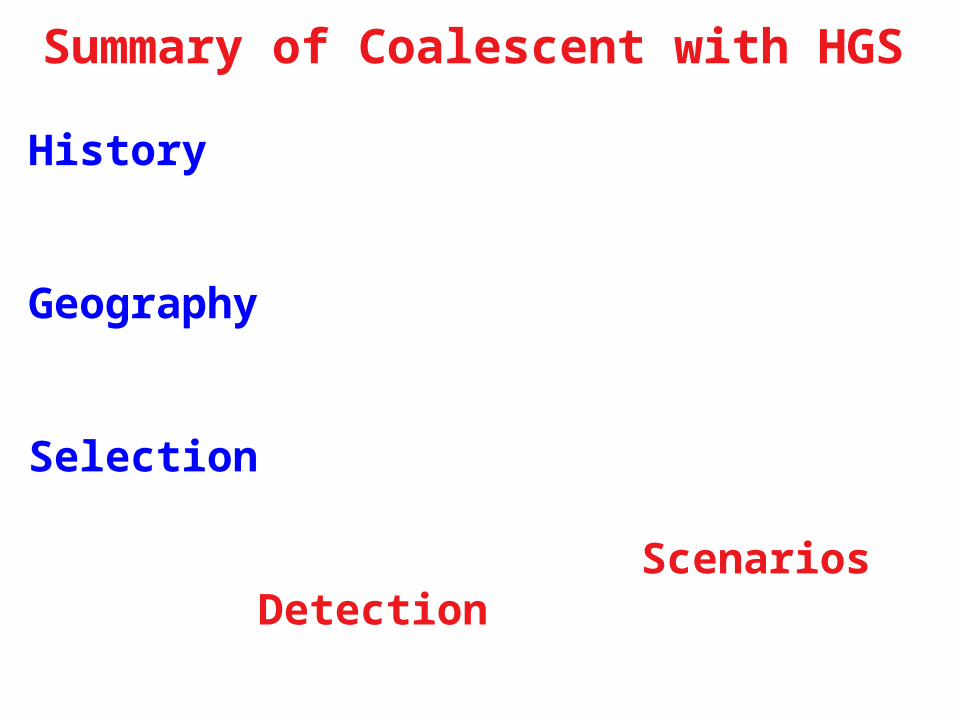
Summary of Coalescent with HGS
History
Geography
Selection
Scenarios Detection

References.(Balding,D. et al. (2000) “Handbook of Statistical Genetics” Wiley Articles by Rousset, Nordborg, Stephens, Hudson,
Barton,NH, Depaulis & Etheridge (2002) Neutral Evolution in Spatially Continuous Populations Theor.Pop.Biol. 61.31-48.Barton, N. & I.Wilson (1996) “Genealogies and Geography” in New uses for New Phylogenies eds. Harvey et al. OUPDonnelly,P., Nordborg, M. & Joyce,P. (2001) Likelihoods and Simulation Methods for Classes of Non-neutral Population Genetics Models. Genetics 159.853-867.
Golding,B. (ed.) (1994) “Non-Neutral Evolution” Chapman & Hall articles by Eanes, Aquadro,.Hudson, McDonald,
Hein,JJ (2002) Slides: www.stats.ox.ac.uk/hein/lectures
Hudson, Boos & Kaplan (1992) A Statistical Test for Detecting Geographical Subdivision” Mol.Biol.Evol. 9.1.138-151
Hudson, Kreitman & Aquade (1987) A test of Neutral Molecular Evolution Based on Nuclear Data. Genetics 116.153-9
Hudson, Darden & Kaplan (1988)
Hudson and Kaplan (1988) “The Coalescent Process in Models with Selection and Recombination” Genetics 120.831-840.
Krone & Neuhauser (1997)
McVean,G. (2002) course: www.stats.ox.ac.uk/mcvean
Neuhauser & Krone (1997) The Genealogy of Samples in Models with Selection Genetics 145.519-534.
Nordborg, M.(1997) “Structured Coalescent Processes on Different Time Scales” Genetics 146.1501-1514.
Pybus,OG et al(2000) An Integrated Framework for the Inference of Viral Population History from Reconstructed Genealogies. Genetics 155.1429-1437.
Schierup, M. et al.(2002) Coalescent Simulator: www.coalescent.dk
Slatkin (1991) Inbreeding Coeffecients and Coalescence Times. Genet. Res. Camb. 58.167-175.
Slatkin & Hudson (1992)
Slade (2000) “Simulation of Selected Genealogies” Theor.Pop.Biol. 57.35-49
Takahata,N.(1990) “A simple genealogical structure of strongly balanced allelic lines of transpecies evolution of polymorphism. PNAS 87.2419-23.
Wiuf, C. and J.Hein (2000) “The Coalescent with Gene Conversion” Genetics 155.451-462.

FST’s & Geography & Coalescent.

History of Coalescent with HGS
Stepping Stone Model introduced by Wright
Krone Neuhauser introduces Selection Graph

Evidence against background selection
From Aquadro, 1994

Evidence for genetic hitch-hiking
From Aquadro, 1994
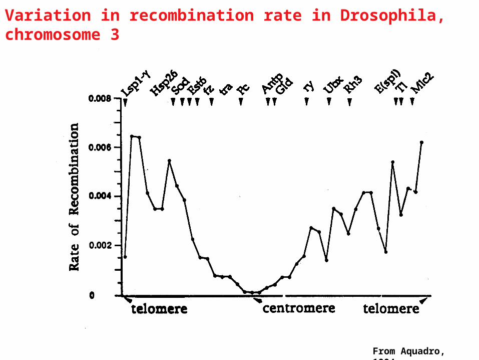
From Aquadro, 1994
Variation in recombination rate in Drosophila, chromosome 3

Selective Sweeps/Background Selection.
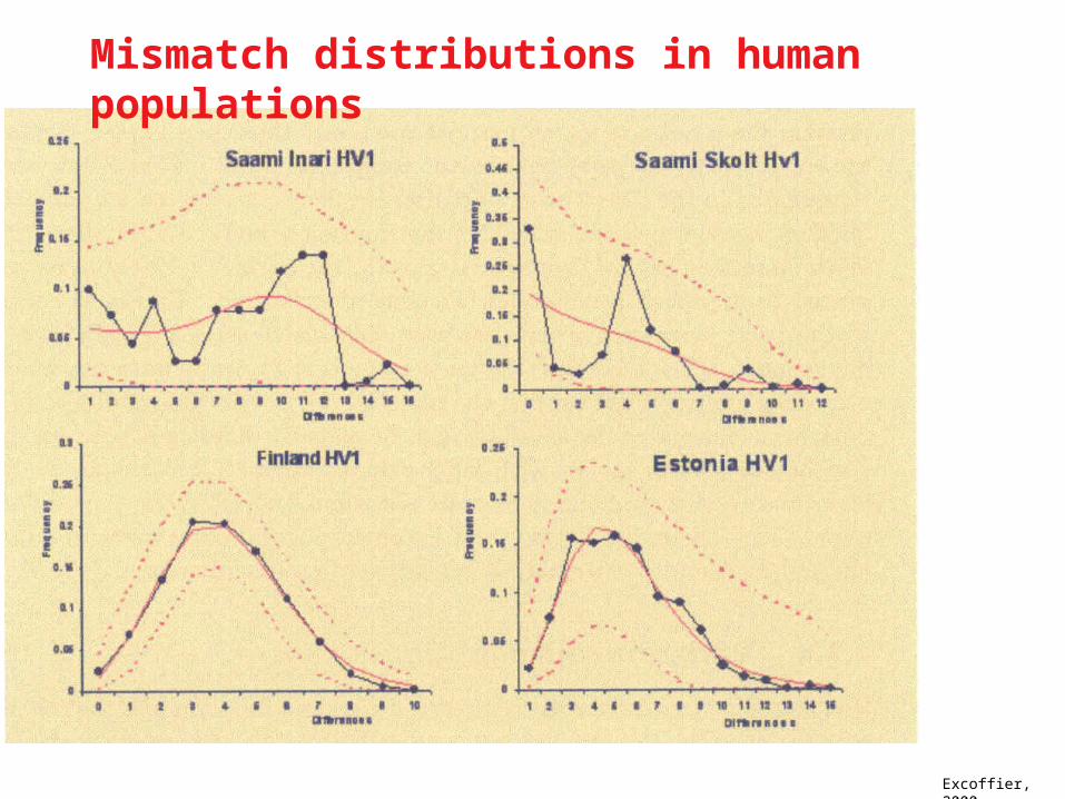
Excoffier, 2000
Mismatch distributions in human populations

External () versus Internal Branches. e and i the number of mutations in external and internal branches.
E() = 2 E() = Lk-2 E(e )= V(e )= E(i )= (Lk-2) V(i )= (Lk-2)/(n-1) + c]
1 if n =2c = b= 2[nLk - 2(n-1)]/(n-1)(n-2)
Fu’s TestFrom Li,1997
1i2
i1
k 1

Waiting intensities in general model of population subdivision