Heiko Schwarz - HHIiphome.hhi.de/schwarz/assets/pdfs/00_Introduction.pdf · Source Coding and...
30
o Source Coding and Compression Heiko Schwarz Contact: Dr.-Ing. Heiko Schwarz [email protected] Heiko Schwarz Source Coding and Compression September 21, 2013 1 / 30
Transcript of Heiko Schwarz - HHIiphome.hhi.de/schwarz/assets/pdfs/00_Introduction.pdf · Source Coding and...
o
Source Coding and CompressionHeiko Schwarz
Contact:
Dr.-Ing. Heiko Schwarz
Heiko Schwarz Source Coding and Compression September 21, 2013 1 / 30

o
Outline
Introduction
Part I: Source Coding Fundamentals
Review: Probability, Random Variables and Random Processes
Lossless Source Coding
Rate-Distortion Theory
Quantization
Predictive Coding
Transform Coding
Part II: Application in Image and Video Coding
Still Image Coding / Intra-Picture Coding
Hybrid Video Coding (From MPEG-2 Video to H.265/HEVC)
Heiko Schwarz Source Coding and Compression September 21, 2013 2 / 30

o
Introduction
Introduction
Display Loudspeaker
Source Encoder
Source Decoder
Demodu- lator
Modu- lator
Channel Encoder
Channel Decoder
Channel
Capture
Heiko Schwarz Source Coding and Compression September 21, 2013 3 / 30
o
Introduction Motivation for Source Coding
Motivation for Source Coding
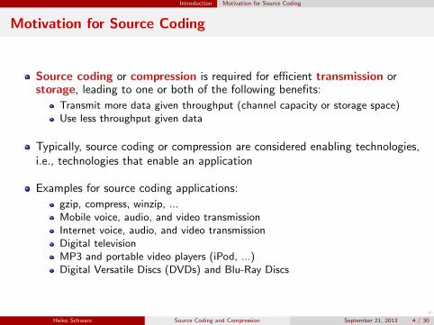
Source coding or compression is required for efficient transmission orstorage, leading to one or both of the following benefits:
Transmit more data given throughput (channel capacity or storage space)Use less throughput given data
Typically, source coding or compression are considered enabling technologies,i.e., technologies that enable an application
Examples for source coding applications:
gzip, compress, winzip, ...Mobile voice, audio, and video transmissionInternet voice, audio, and video transmissionDigital televisionMP3 and portable video players (iPod, ...)Digital Versatile Discs (DVDs) and Blu-Ray Discs
Heiko Schwarz Source Coding and Compression September 21, 2013 4 / 30

o
Introduction Motivation for Source Coding
Practical Source Coding Problems
File compression (text file, office document, program code, ...)Example: Example 80 MByte down to 20 MByte (20%)
Audio compressionStereo with sampling frequency of 44.1 kHzEach sample being represented with 16 bits
=⇒ Raw data rate: 44.1×16×2 = 1.41 Mbit/s=⇒ Typical data rate after compression: 64 kbit/s (4.5%)
Image compressionOriginal picture size: 3000×2000 samples (6 MegaPixel)3 color components (red, green, blue) and 1 byte (8 bit) per sample
=⇒ Raw file size: 3000×2000×3 = 18 MByte=⇒ Typical compressed file size: 1 MByte (5.6%)
Video compressionPicture size of 1920×1080 pixels and frame rate of 50 HzEach sample being digitized with 8 bit3 color components (red, green, blue)
=⇒ Raw data rate: 1920×1080×8×50×3 = 2.49 Gbit/s=⇒ Typical compressed data rate: 12 Mbit/s (0.5%)
Heiko Schwarz Source Coding and Compression September 21, 2013 5 / 30
o
Introduction Motivation for Source Coding
Source Coding in Practice
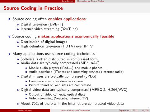
Source coding often enables applications:
Digital television (DVB-T)Internet video streaming (YouTube)
Source coding makes applications economically feasible
Distribution of digital imagesHigh definition television (HDTV) over IPTV
Many applications use source coding techniques
Software is often distributed in compressed formAudio data are typically compressed (MP3, AAC)
Mobile audio players (IPod,...) and mobile phonesAudio download (ITunes) and streaming services (Internet radio)
Digital images are typically compressed (JPEG)
Compression is often done in cameraPicture found on web sites are compressed
Digital video data are typically compressed (MPEG-2, H.264/AVC)
Output of video cameras, optical discsVideo streaming (Youtube, Internet TV)
About 70% of the bits in the Internet are compressed video data
Heiko Schwarz Source Coding and Compression September 21, 2013 6 / 30

o
Introduction Analog-to-Digital Conversion
Pulse-Code Modulation
Analog-to-Digital Conversion: Pulse-Code Modulation
Pulse-code modulation (PCM) is based on following principles
Sampling (obeying Shannon-Nyquist sampling theorem)Quantizing sample values
Sampling theorem asserts that a time-continuous signal s(t) that containsonly frequencies less than Ω Hz, can be recovered from a sequence of itssample values using
s(t) =
∞∑n=−∞
s(tn)ψ(t− tn) (1)
where s(tn) is value of nth sampling instant tn = n2Ω and ψ(·) is given as
ψ(t) =sin(2πΩt)
2πΩt(2)
The signal values s(tn) can be quantized allowing only an approximatereconstruction of s(t)
Heiko Schwarz Source Coding and Compression September 21, 2013 7 / 30
o
Introduction Analog-to-Digital Conversion
Analog-to-Digital Conversion: Overview
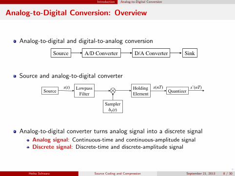
Analog-to-digital and digital-to-analog conversion
Source A/D Converter D/A Converter Sink
Source and analog-to-digital converter
Source Lowpass Filter
Sampler δT(t)
Holding Element Quantizer
s(t) s(nT) s’(nT)
Analog-to-digital converter turns analog signal into a discrete signal
Analog signal: Continuous-time and continuous-amplitude signalDiscrete signal: Discrete-time and discrete-amplitude signal
Heiko Schwarz Source Coding and Compression September 21, 2013 8 / 30

o
Introduction Analog-to-Digital Conversion
Analog-to-Digital Conversion
Source Lowpass Filter
Sampler δT(t)
Holding Element Quantizer
s(t) s(nT) s’(nT)
Sample and hold operator turns continuous-time into discrete-time signal
Low-pass filter ensures that signal is band-limited
Quantizer turns continuous-amplitude signal into discrete-amplitude signal
A simple method is to quantize signal s(nT ) by mapping it to K = 2k
possible amplitude valuesA simple quantization rule is
s′(nT ) = bs(nT )× 2k + 0.5c/2k (3)
We use the notation for the discrete signal s[n] as an abbreviation for s′(nT )with T being the sampling interval
Digital values s[n] are in practice numbers that are stored in a computer
Heiko Schwarz Source Coding and Compression September 21, 2013 9 / 30
o
Introduction Analog-to-Digital Conversion
Why Analog-to-Digital Conversion?
Required for processing data with a computer
All compression methods discussed here are computer programs:
Encoder: Mapping of s[n] into a bit stream bDecoder: Mapping of the bit stream b into the discrete decoded signal s′[n]
Although we will also discuss compression of analog signals in theory, inpractice all algorithms will assume discrete versions of these analog signalsthat are very close approximation of these analog signals
Heiko Schwarz Source Coding and Compression September 21, 2013 10 / 30
o
Introduction Analog-to-Digital Conversion
One-Dimensional Signal Example
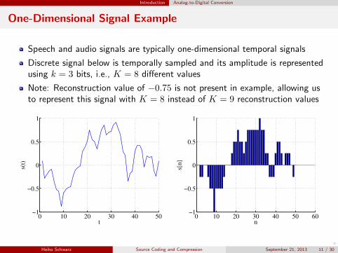
Speech and audio signals are typically one-dimensional temporal signals
Discrete signal below is temporally sampled and its amplitude is representedusing k = 3 bits, i.e., K = 8 different values
Note: Reconstruction value of −0.75 is not present in example, allowing usto represent this signal with K = 8 instead of K = 9 reconstruction values
0 10 20 30 40 50−1
−0.5
0
0.5
1
t
s(t)
0 10 20 30 40 50 60−1
−0.5
0
0.5
1
n
s[n
]
Heiko Schwarz Source Coding and Compression September 21, 2013 11 / 30

o
Introduction Analog-to-Digital Conversion
Two-Dimensional Signal Example
Pictures are two-dimensional spatial signals
Videos are three-dimensional spatio-temporal signals
Below sampling of picture Lena with different spatial sampling rates
8× 8, 16× 16, 32× 32, and 128× 128 samples (from left to right)Each sample is represented with n = 8 bitsEach square represents average of luminance values it covers
Heiko Schwarz Source Coding and Compression September 21, 2013 12 / 30

o
Introduction Analog-to-Digital Conversion
Two-Dimensional Signal Example
Below quantization of picture Lena with different bits/sample
k = 1, 2, 4, and 8 bits/sample (from left to right)The spatial sampling rate is fixed to 128×128
Heiko Schwarz Source Coding and Compression September 21, 2013 13 / 30

o
Introduction Analog-to-Digital Conversion
Three-Dimensional Signal Examples
Below, format, sampling rate and sampling method for different video signalsyield corresponding PCM data rates
Picture format Luma signal Chroma signal Sampling Frames/s Data rate
Common Intermediate 352× 288 2× 176× 144 progressive 25Format (CIF) (352× 240) (2× 176× 120) 8 bit (30)
ITU-R BT.601 Format 720× 576 2× 360× 576 interlaced 25(“Standard Television”) (720× 480) (2× 360× 480) 8 bit (30)
ITU-R BT.709: 720p 1280× 720 2× 640× 720 progressive 50(“High Definition TV”) 8 bit (60)
ITU-R BT.709: 1080i 1920× 1080 2× 960× 1080 interlaced 25(“Full HDTV”) 8 bit (30)
ITU-R BT.2020: UHD-1 3840× 2160 2× 1920× 1080 progressive 50(“Ultra HDTV 4k”) 10 bit (60)
ITU-R BT.2020: UHD-2 7680× 4320 2× 3840× 2160 progressive 50(“Ultra HDTV 8k”) 12 bit (60)
Heiko Schwarz Source Coding and Compression September 21, 2013 14 / 30

o
Introduction Communication Problem
Basic Communication Problem
The basic communication problem may be posed as
Conveying source data with highest fidelity possiblewithin an available bit rate
or, equivalently, as
Conveying source data using lowest bit rate possiblewhile maintaining a specified reproduction fidelity
In either case, a fundamental trade-off is made between bit rate and fidelity
The ability of a source coding system to make this trade-off well is called itscoding efficiency or rate-distortion performance, and the coding systemitself is referred to as a source codec
Source codec: a system comprising a source coder and a source decoder
Heiko Schwarz Source Coding and Compression September 21, 2013 15 / 30

o
Introduction Communication Problem
Example: JPEG (1:10 Compression)
Heiko Schwarz Source Coding and Compression September 21, 2013 16 / 30
o
Introduction Communication Problem
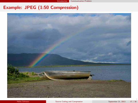
Example: JPEG (1:50 Compression)
Heiko Schwarz Source Coding and Compression September 21, 2013 17 / 30

o
Introduction Communication Problem
Example: H.265/HEVC (1:50 Compression)
Heiko Schwarz Source Coding and Compression September 21, 2013 18 / 30
o
Introduction Communication Problem
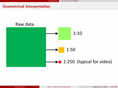
Geometrical Interpretation
Raw data
1:10
1:50
1:250 (typical for video)
Heiko Schwarz Source Coding and Compression September 21, 2013 19 / 30

o
Introduction Communication Problem
Transmission System
Display Loudspeaker
Source Encoder
Source Decoder
Demodu- lator
Modu- lator
Channel Encoder
Channel Decoder
Channel
Capture
Heiko Schwarz Source Coding and Compression September 21, 2013 20 / 30

o
Introduction Communication Problem
Practical Communication Problem
Source codecs are primarily characterized in terms of:
Throughput of the channel, a characteristic influenced by
transmission channel bit rate and
amount of protocol and error-correction coding overhead incurred bytransmission system
Distortion of the decoded signal, which is primarily induced by
source encoder and
by channel errors introduced in path to source decoder
The following additional constraints must also be considered
Delay (start-up latency and end-to-end delay) include
processing delay, buffering,structural delays of source and channel codecs, andspeed at which data are conveyed through transmission channel
Complexity (computation, memory capacity, memory access) of
source codec,protocol stacks, and network
Heiko Schwarz Source Coding and Compression September 21, 2013 21 / 30

o
Introduction Communication Problem
Formulation of the Practical Communication Problem
The practical source coding design problem is posed as follows:
Given a maximum allowed delay and a maximumallowed complexity, achieve an optimal trade-offbetween bit rate and distortion for the transmissionproblem in the targeted applications.
Here, we will concentrate on source codec only
Delay is only evaluated for source codec
Complexity is also only assessed for the algorithm used in source codec
Heiko Schwarz Source Coding and Compression September 21, 2013 22 / 30

o
Introduction Communication Problem
Scope of This Course
Heiko Schwarz Source Coding and Compression September 21, 2013 23 / 30

o
Introduction Communication Problem
Transmission Channels and Optical Storage Media
Fixed transmission lines:
ISDN line: 64 kbit/sADSL: 6 Mbit/sVDSL: 25 Mbit/s or 50 Mbit/s
Mobile networks:
GSM: 15 kbit/sEDGE: 474 kbit/s (max)HSDPA: 7.2 Mbit/s (peak)LTE: 300 Mbit/s (peak)
Broadcast channels
DVB-T: 13 Mbit/s (16QAM)DVB-S: 38 Mbit/s (QPSK)DVB-C: 38 Mbit/s (64QAM)
Optical storage media
Compact Disc (CD): 650 MByte with 1.41 Mbit/s (12 cm)Digital Versatile Dics (DVD): 4.7 GByte with 10.5 Mbit/s (DVD-5-SS-SL)Blu-Ray Disc (BRD): 50 GByte with 36 Mbit/s (12 cm, DS-DL)
Heiko Schwarz Source Coding and Compression September 21, 2013 24 / 30

o
Introduction Communication Problem
Types of Compression
Lossless coding:
Uses redundancy reduction as the only principle and is therefore reversible
Also referred to as noiseless or invertible coding or data compaction
Well known use for this type of compression for data is Lempel-Ziv coding(gzip) and for picture and video signals JPEG-LS is well known
Lossy coding:
Uses redundancy reduction and irrelevancy reduction and is therefore notreversible
It is the primary coding type in compression for speech, audio, picture, andvideo signals
The practically relevant bit rate reduction that is achievable through lossycompression is typically more than an order of magnitude larger than withlossless compression
Well known examples are for audio coding are the MPEG-1 Layer 3 (mp3), forstill picture coding JPEG, and for video coding H.264/AVC
Heiko Schwarz Source Coding and Compression September 21, 2013 25 / 30
o
Introduction Distortion/Quality Measures
Distortion Measures
The use of lossy compression requires the ability to measure distortion
Often, the distortion that a human perceives in coded content is a verydifficult quantity to measure, as the characteristics of human perception arecomplex
Perceptual models are far more advanced for speech and audio codecs thanfor picture or video codecs
In speech and audio coding,
Perceptual models are heavily used to guide encoding decisionsListening tests are used to determine subjective quality of coding results
In picture and video coding,
Perceptual models have limited use to guide encoding decisions (mainlyfocusing on properties of the human visual system)Viewing tests are used to determine subjective quality of coding results
This lecture: Use of objective distortion measures such as MSE and SNR
Heiko Schwarz Source Coding and Compression September 21, 2013 26 / 30

o
Introduction Distortion/Quality Measures
Mean Squared Error (MSE)
Speech and audio: (N : duration in samples)
u[n] = s′[n] − s[n] (4)
MSE =1
N
N−1∑n=0
u2[n] (5)
Pictures: (X: picture height, Y : picture width):
u[x, y] = s′[x, y] − s[x, y] (6)
MSE =1
X · Y
X−1∑x=0
Y−1∑y=0
u2[x, y] (7)
Videos: (N : number of pictures, MSEn: MSE of picture n):
MSE =1
N
N−1∑n=0
MSEn (8)
Heiko Schwarz Source Coding and Compression September 21, 2013 27 / 30

o
Introduction Distortion/Quality Measures
Signal-to-Noise Ratio
Speech:
SNR = 10 · log10
(σ2
σ2u
)(9)
with σ2 =1
N
N−1∑n=0
(s[n] − µs)2 and µs =
1
N
N−1∑n=0
s[n] (10)
σ2u =
1
N
N−1∑n=0
(u[n] − µu)2 and µu =1
N
N−1∑n=0
u[n] (11)
Pictures: (k: bit depth of samples)
PSNR = 10 · log10
((2k − 1)2
MSE
)(12)
Videos: (N : number of pictures, PSNRn: PSNR of picture n)
PSNR =1
N
N−1∑n=0
PSNRn (13)
Heiko Schwarz Source Coding and Compression September 21, 2013 28 / 30

o
Introduction Literature
Recommended Literature
Source Coding
T. M. Cover and J. A. Thomas, “Elements of Information Theory,” John Wiley & Sons,New York, 1991.
Gersho, A. and Gray, R. M. (1992), “Vector Quantization and Signal Compression,” KluwerAcademic Publishers, Boston, Dordrecht, London.
Jayant, N. S. and Noll, P. (1994), “Digital Coding of Waveforms,” Prentice-Hall,Englewood Cliffs, NJ, USA.
Wiegand, T. and Schwarz, H. (2010). Source Coding: Part I of Fundamentals of Sourceand Video Coding, Foundations and Trends in Signal Processing, vol. 4, no. 1-2.(http://iphome.hhi.de/wiegand/assets/pdfs/VBpart1.pdf)
Image and Video Coding
W. Pennebaker and J. Mitchell, “JPEG Still Image Data Compression Standard,” VanNostrand Reinhold, New York, 1993.
D. S. Taubman and M. W. Marcellin, “JPEG 2000 – Image Compression Fundamentals,Standards, and Practice,” Kluwer Academic Publishers, 2002.
Y. Wang, J. Ostermann, Y.-Q. Zhang, “Video Processing and Communications,”Prentice-Hall, 2002.
J.-R. Ohm, “Multimedia Communication Technology. Representation, Transmission andIdentification of Multimedia Signals,” Springer, Heidelberg/Berlin, 2004.
Heiko Schwarz Source Coding and Compression September 21, 2013 29 / 30

o
Introduction Organization
Organization
Lecture: Tuesday 10:30-12:00 & 12:15-13:45Room 1.16
Lecturer: Dr.-Ing. Heiko Schwarz
Head, Image & Video Coding GroupImage Processing DepartmentFraunhofer Heinrich Hertz Institute
[email protected]://iphome.hhi.de/schwarz
Course weights: Quizzes: 20%Project: 20%Midterm exam: 25%Final exam: 35%
Copies of slides and solutions of exercises can be downloaded at:
http://iphome.hhi.de/schwarz/GUC-SourceCoding.htm
Heiko Schwarz Source Coding and Compression September 21, 2013 30 / 30