Hedging Price Risk in the Presence of Crop Yield and Revenue Insurance

Olivier Mahul e-mail: mahul@roazhon.inra.fr

Paper prepared for presentation at the Xth EAAE Congress ‘Exploring Diversity in the European Agri -Food System’,

Zaragoza (Spain), 28-31 August 2002

Copyright 2002 by Olivier Mahul. All rights reserved. Readers may make verbatim copies of this document for non-commercial purposes by any means, provided that this

copyright notice appears on all such copies.

Hedging Price Risk in the Presence of Crop Yield and Revenue Insurance

Olivier Mahul

INRA, Department of Economics

Rue Adolphe Bobierre CS 61103

35011 Rennes Cedex France

Email : mahul@roazhon.inra.fr

First draft: January 2002

1

Hedging Price Risk in the Presence of Crop Yield and Revenue Insurance

Abstract The demand for hedging against price uncertainty in the presence of crop yield and revenue insurance contracts is examined for two French wheat farms. The rationale for the use of options in addition to futures is first highlighted through the characterization of the first-best hedging strategy in the expected utility framework. It is then illustrated using numerical simulations. The presence of options is shown to allow the insured producer to adopt a more speculative position on the futures market. Futures are shown to be performing, in terms of willingness to receive. Options are weakly performing when futures markets are unbiased, while they are more performing when futures markets are biased.

Key words: crop insurance, hedging, producer welfare, simulation.

2

1. Introduction

The agricultural sector is characterized by a strong exposure to risk which is still likely to increase in the near future. Production risk is expected to increase due to stricter uses as regards the use of inputs creating potential environmental damages. Price risk is likely to rise because of agricultural trade liberalization. In Europe, this increasing price volatility would be induced by the recent reforms of the Common Agricultural Policy. Meanwhile, insurance or hedging contracts which allow European farmers to manage price and yield uncertainty are limited. For example, French farmers can only buy named-peril insurance contracts (against hail, storm and frost) and hedging contracts against price risk proposed by the European board of trade EURONEXT are still confidential. This induces the private and public markets to examine the development of new hedging and insurance instruments. In particular, they wish to investigate the substituability/complementarity between crop yield and revenue insurance programs and hedging contracts against price risk.

There is a growing literature on optimal hedging under price and quantity uncertainty. In a pioneering work, McKinnon (1967) reports that hedge ratios minimizing the variance decline as yield variability relative to price variability increases. Rolfo (1980) shows that the ratio of optimal futures hedge to expected output should be below unity for individuals with a logarithmic utility function. Losq (1982) generalizes this result when price and output are independent and the marginal utility function is convex. More recently, Lapan and Moschini (1995) analyze optimal hedging decisions for firms facing price, basis and production risk, assuming futures and options (at a single strike price) can be used. Under restrictive assumptions on the producer’s behavior towards risk and on the yield and price distributions, they show that production risk provides a rationale for the use of options. This finding is extended by Mahul (2002) from the characterization of the first-best hedging solution.

The purpose of this paper is to investigate the demand for hedging against price risk in the presence of crop yield and revenue insurance contracts using numerical simulations. The main originality of this paper is to allow insured producers to use options at different strike prices in addition to futures. The design of the optimal hedging instrument is first analyzed in the expected utility framework when the producer is endowed with a crop yield insurance or a crop revenue insurance policy. The rationale for the use of options is highlighted from the non-linearity of the first-best solution. In the simulation model, five mutually exclusive agricultural insurance policies are modeled: individual and aggregate crop yield insurance, individual and aggregate crop revenue insurance, and the U.S. Crop Revenue Coverage. The insured producer has also the opportunity to buy or sell futures and options on futures. Contrary to recent empirical studies (see, for example, Wang et al., 1998; Coble, Heifner and Zuniga, 2000), options contracts available at different strike prices can be jointly used with futures. The optimal hedging positions under every insurance policy are evaluated for two French wheat farms. They stress the role of futures, in addition to yield or revenue insurance policy, to reduce revenue uncertainty. The shape of the optimal hedging strategy is then derived from these hedge ratios. The impact of perceived bias in futures prices at harvest on optimal hedging decisions is examined through a decomposition of the hedge ratio. The effect of insurance guarantee level on the optimal futures and straddles positions is also evaluated. The performance of the optimal combination between insurance policies and financial instruments is investigated through the evaluation of a willingness to receive measure. A conclusion highlights the main results and discusses several extensions to this work.

3

2. Some Remarks on Optimal Hedging Contract under Production and Price Uncertainty

We consider a competitive farmer/producer who makes all insurance and hedging decisions at the beginning of the period (at planting), whereas all uncertainty is resolved at the end of the period (at harvest). The farmer is assumed to produce a single commodity and he faces production and price uncertainty. This implies that the exact output and the exact price at which he sells his output (the individual cash price) are unknown at the beginning of the period. Production risk and price risk are formally represented by positive random variables y~ and p~ , respectively.1 The cost function depends on the expected output yEy ~= , where E denotes the expectation operator, and it is denoted ( )yc . The expected production is related to planted acreage (normalized to unity) and intensity of other inputs which are given parameters in this one-period model. They are assumed to be known at the beginning of the period. The purpose of this section is to examine the impact of insurance contract on the hedging demand. Consequently, two assumptions are made for the ease of the analysis: (i) production and price risks are stochastically independent and (ii) insurance and hedging contracts are based on individual production and individual cash price. Assumption (i) means that the systemic component in production uncertainty is not large enough to affect the output price. Assumption (ii) means that the model is free of yield basis risk and price basis risk. Both assumptions will be removed in the simulation model.

The producer is assumed to be risk averse, with preferences represented by an increasing and concave von Neumann-Morgenstern utility function u .2 He is endowed with an insurance contract that consists of an indemnity payoff net of the premium denoted . This net indemnity schedule is based on yield under crop yield insurance,

NI( )yNI , and on gross revenue

under crop revenue insurance, . The design of the first-best hedging instrument against price risk is examined. It is described by the couple

(pyNI )[ ]P(.),J where ( )pJ is the non-negative

payoff when the realized price is p and ( ) ( )EJ pP ~1 λ+= , where 0≥λ is the loading rate, is the premium which is assumed to be proportional to the expected payoff. The first-best solution maximizes the producer’s expected utility of final wealth under the above-mentioned constraints:

( )( )π~

.EuMax

J (1)

subject to and ( ) 0. ≥J ( ) ( )pEJP ~1 λ+= , where π~ is the producer’s final wealth corresponding to

( ) ( ) ( ) PpJyNIycyp −++−= ~~~~~π (2) when he is endowed with the crop yield insurance contract and

( ) ( ) ( ) PpJypNIycyp −++−= ~~~~~~π (3) when the revenue insurance policy is available.

Under crop yield insurance, the indemnity schedule is independent of the random output price. The production risk can thus be interpreted as an independent (multiplicative) background risk. From Mahul (2002), the first-best indemnity schedule can be shown to be decreasing when

1 Random variables are denoted with a tilde, their realizations without. 2 The producer may be risk neutral but he may behave as if he were risk averse. His (apparent) risk aversion may be due to market imperfections (Greenwald and Stiglitz, 1993), to the direct and indirect costs of financial distress, to the existence of taxes that are a convex function of earnings (Smith and Stulz, 1985), or to information asymmetries that raise the cost of external funds relative to internal funds (e.g., Smith and Stulz, 1985; Froot, Scharfstein and Stein, 1993).

4

the realized price is lower than a strike price , and it is zero otherwise. The first-best marginal payoff function satisfies:

p

( ) ( )[ ]( )

( )( )( )π

πππ

~~,~cov

~~~

uEuyy

uEuyEpJ

′′′′

−−=′′′′

−=′ for all pp ˆ< , (4)

where ( ) ( ) ( ) PpJyNIycyp −++−= ~~~π and is the covariance operator. Contrary to the case with no crop insurance examined by Mahul (2002), it should be noticed that

cov

( )yINpy ′+=∂∂π can be either positive or negative without any additional assumption of the crop yield insurance policy. Suppose that ( ) [ ] QyyyNI −−= 0,ˆmaxδ where is the yield guarantee,

yδ is the price election and is the insurance premium. Therefore Q y∂∂π will be

positive for all and all y δ>p . The covariance term is thus positive if the producer exhibits prudence, u .0>′′′ 3 The first-best marginal payoff thus satisfies:

( ) ypJ −>′ for all ] pp ˆ, [δ∈ with p<δ . (5) The sign of the covariance term is indeterminate otherwise. This covariance term vanishes if the utility function is quadratic, .0=′′′u 4 We thus have ( ) ypJ −=′ for all . This implies that the optimal hedging instrument is

( ) 0: >pJp( ) [ ]0,ˆmax ppypJ −= where is the strike price. This

is equivalent to buying p

y put options at strike price . Consequently, introducing a crop yield insurance contract does not affect the form of the first-best hedging contract under a quadratic utility function. Obviously, the optimal strike price will be altered. When the utility function is not quadratic, we deduce from equation (4) that the first-best hedging contract is not linear in the price. This thus provides a rationale for the use of options in order to replicate as close as possible this non-linearity.

p

When the producer is endowed with a revenue insurance contract, it can be shown (see the Appendix) that there exists a strike price under which indemnity payoffs are made and first-best marginal payoff function satisfies

p

( ) ( )( ) ( )[ ]( ) ( )( )[ ] ( )( ) ( )( )

( )ππ

ππ

~~,~1~cov~1~

~~~1~

uEuypINyypINyE

uEuypINyEpJ

′′′′′+

−′+−=′′

′′′+−=′ (6)

for all , where pp ˆ< ( ) ( ) ( ) PpJypNIycyp −++−= ~~~π . When the (apparent) utility function is quadratic, the covariance term in (6) vanishes.

Contrary to the crop yield insurance case, the first right-hand side term in (6) depends on the revenue insurance contract through its marginal indemnity function. If the revenue insurance schedule satisfies ( ) [ ] QpyRpyNI −−= 0,ˆmax where R is the revenue guarantee and is the insurance premium, then we have

Q

( ) ( )( )[ ] [ ]( )pRyyypINyEpJ /ˆ~Prob1~1~ <−−=′+−=′ , (7) for all . The slope of the first-best hedging contract thus clearly depends on the revenue guarantee

pp ˆ<

R . Under the general case where the utility function is not quadratic, the covariance term in (7)

is positive if the insured producer is not over-indemnified when a loss occurs, i.e., ( ) 1−≥′ pyIN

3 The convexity of the marginal utility, u , has long been recognized has a realistic behavioral assumption. It is a necessary condition for decreasing absolute risk aversion. It is a necessary and sufficient condition for an increase in future income risk to induce consumers to save more (Kimball, 1990).

0>′′′

4 The limitations of this utility function to represent attitudes towards risk are well-known (e.g., the index of absolute risk aversion increases with wealth). However, this function can also represent a risk-neutral producer facing a quadratic and convex tax schedule.

5

where the weak inequality is strict at some py under partial insurance. The first-best marginal payoff thus satisfies

( ) ( )([ ypINyEpJ )]~1~ ′+−>′ , (8) for all . The marginal payoff function expressed in (6) stresses the non-linearity of the first-best hedging instrument with respect to the output price. This gives a rationale for the use of option, not only when the utility function is non-quadratic, as in the crop yield insurance case, but also when it is quadratic.

pp ˆ<

3. The Simulation Model

3.1. Insurance and Hedging Contracts Offered

We aim at investigating the role of insurance and financial markets in the management of production and price risk in agriculture through a simulation model. Five insurance products and four hedging contracts are modeled in order to reflect the products that are currently offered to the U.S. farmers and that may be offered to the French farmers in the near future.

In the insurance market, two crop yield insurance policies and three crop revenue insurance contracts are assumed to be at the producer’s disposal. These contracts are mutually exclusive and they are sold at an actuarially fair price.5

Among the crop yield insurance programs, we consider the Individual Yield Crop Insurance (IYCI) contract in which the indemnity is based on individual yield, denoted . Formally, the IYCI indemnity schedule net of the premium satisfies:

y

( ) [ ] IYCIIYCI QyyEFyNI −−= 0,~max γδ , (9) where is the futures price at planting, F δ is a fraction of this price, γ is a percentage of the expected individual yield, and Q is the insurance premium. This contract corresponds to the multiple peril crop insurance program offered to the U.S. farmers. The second crop yield insurance contract is based on aggregate yield of a surrounding area, denoted . It is called Area Yield Crop Insurance (AYCI) and its net indemnity schedule is

IYCI

q

( ) [ ] AYCIAYCI QqqEFqNI −−= 0,~max φδ , (10)

where qE~ is the expected area yield, φ is a percentage of the expected area yield and is the associated premium. Such a contract has been widely examined in the literature (see, for example, Miranda, 1991; Skees, Black and Barnett, 1997; Mahul, 1999; Vercammen, 2000). It is less exposed to asymmetric information problems, i.e., moral hazard and adverse selection, because farmers cannot alter the indemnity and information about area yield are usually more easily available and more accurate than information about individual yield. However, this contract does not provide a coverage against yield basis risk generated by the imperfect correlation between individual and area yields. It looks like the insurance policy offered by the Group Risk Plan to the U.S. farmers.

AYCIQ

Three different revenue insurance policies are under consideration. Contrary to crop yield insurance programs, they provide a coverage for both yield and price uncertainty. Under the Individual Revenue Insurance (IRI) contract, the net indemnity schedule is

( ) [ ] IRIIRI QfyyFEfyNI −−= 0,~max γ , (11) where is the futures price at harvest, f γ is a percentage of the expected individual revenue

yFE~ and is the insurance premium. It looks like the Revenue Assurance and Income IRIQ

5 We thus implicitly assume that these insurance programs are subsidized.

6

Protection programs proposed to the U.S. farmers. In the spirit of the AYCI contract, the indemnity payoff of the Area Revenue Insurance (ARI) policy is defined as

( ) [ ] ARIARI QfqqEFfqNI −−= 0,~max φ , (12)

where is the associated premium. This policy looks like the new U.S. insurance product introduced as a pilot program in 1999, called Group Risk Income Protection (Barnett, 2001). Finally, the Crop Revenue Coverage (CRC) contract, which has the highest enrollment among the U.S. farmers, is considered. Its main originality is to provide a replacement-cost protection when yields are low and prices are high. Its indemnity net of the premium Q is

ARIQ

CRC

( ) ( )[ CRCCRC QfyyEfFyfNI −−= 0, ]~,maxmax, γ . (13) It is noteworthy that the indemnity schedules of the three revenue insurance programs are based on futures prices and not individual cash prices. This means that the producer is exposed to price basis risk caused by the imperfect correlation between individual cash and futures prices.

Since the purpose of this paper is to examine the demand for hedging, producers have not the possibility to choose the percentage yield guarantees and the coverage level. We assume that

1=δ , i.e., the price election is equal to the futures price at harvest perceived by the agents; %80=γ , i.e., the individual yield guarantee under IYCI, IRI and CRC is 80 percent of the

expected individual yield (20% deductible); %90=φ , i.e., the area yield guarantee under AYCI and ARI is 90 percent of the expected area yield (10% deductible). This difference in yield guarantees between insurance contracts based on individual or area yields is justified as follows. Individual yield and revenue insurance contracts provide a (partial) coverage against the whole individual yield risk, whereas area yield and revenue policies only offer a (partial) coverage against the systemic component of the individual yield risk. For a given level of yield guarantee, this implies that producers will prefer actuarially fair contracts based on individual yields rather than area yields. In addition, maximum on yield guarantee is usually justified to mitigate moral hazard problems (introducing a deductible would induce insured producers not to alter their preventive behavior towards risk). This problem is significantly reduced under area yield or revenue insurance because producers cannot alter the indemnity based upon area yield. Consequently, it seems realistic to assume that φ is higher than γ .

Real-world financial markets offer standardized forms of hedging contracts, such as futures contracts and options on futures. Since these tools are linear or piecewise linear with the price, it should be noticed that they usually preclude the replication of the first-best hedging instrument as expressed in equations (4) and (6). This creates a second source of incompleteness on financial markets, in addition to price basis risk. Following Mahul (2002), we assume that the producer has the opportunity to buy or sell not only futures but also options on futures available are different strike prices. We restrict our attention to the case where straddles at three different strike prices are available.6 We denote k for i 3,2,1=i the strike price where , the futures quantity sold, for

321 kkk << 0>x0>iz 3,2,1=i the quantity of straddles at strike price sold, and

for i the associated straddle premium. The hedging strategy is thus defined as ik

iP 3,2,1=

( ) [ ] [∑=

−−+−=3

1iiii kfPzfFxfS ]

. (14)

It is piecewise linear with three kinks at each strike price and its first derivative is

6 A short (resp. long) straddle can be constructed by selling (resp. buying) one put and one call at the same strike price.

7

( )

>−−−−<<+−−−<<++−−

<+++−

=′

3321

32321

21321

1321

if if if if

kfzzzxkfkzzzxkfkzzzx

kfzzzx

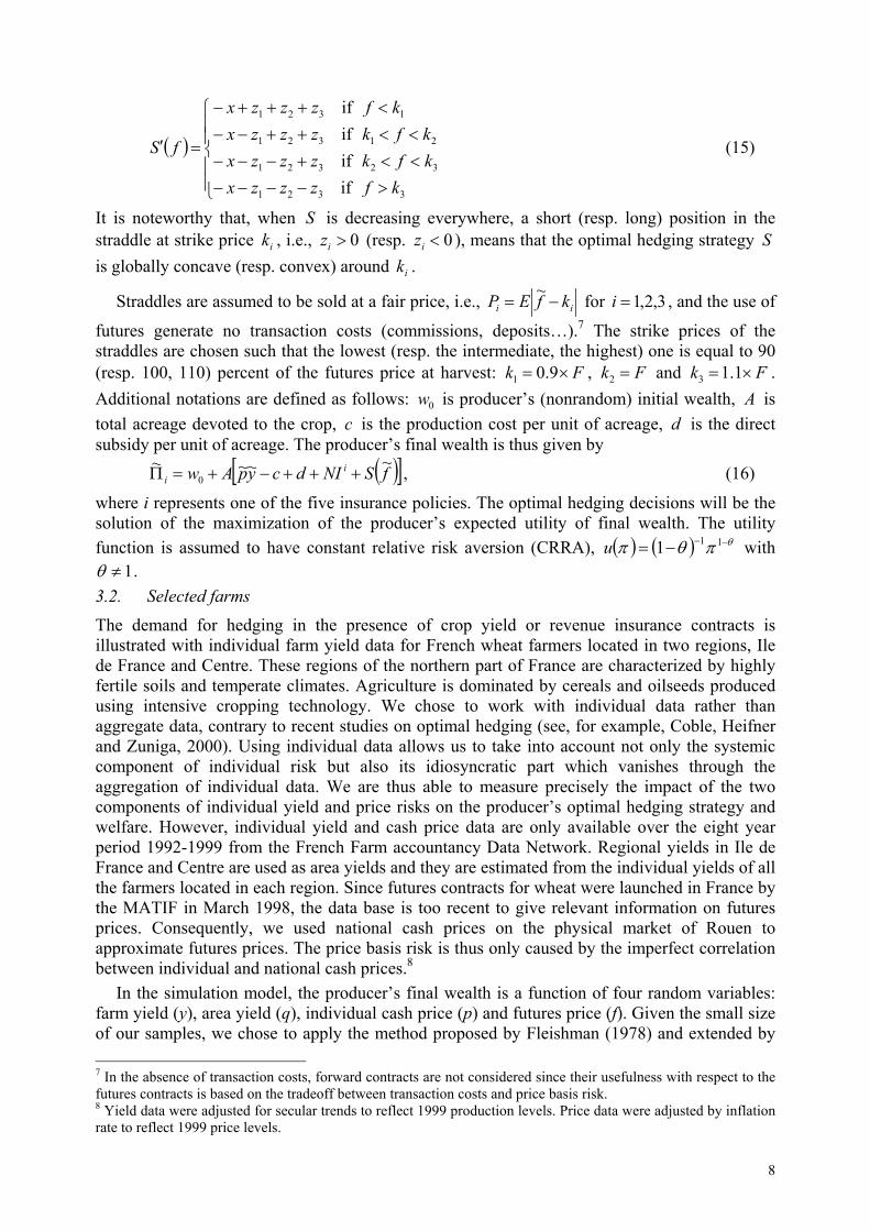
fS (15)

It is noteworthy that, when is decreasing everywhere, a short (resp. long) position in the straddle at strike price k , i.e., (resp.

Si 0>iz 0<iz ), means that the optimal hedging strategy

is globally concave (resp. convex) around k . S

i

Straddles are assumed to be sold at a fair price, i.e., ii kfEP −=~ for , and the use of

futures generate no transaction costs (commissions, deposits…).

3,2,1=i7 The strike prices of the

straddles are chosen such that the lowest (resp. the intermediate, the highest) one is equal to 90 (resp. 100, 110) percent of the futures price at harvest: Fk ×= 9.01 , and kF=2k F×= 1.13

A.

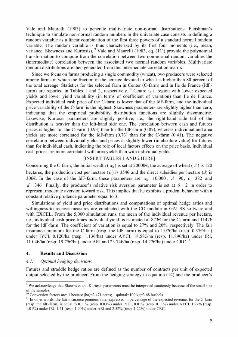
Additional notations are defined as follows: is producer’s (nonrandom) initial wealth, is total acreage devoted to the crop, is the production cost per unit of acreage, d is the direct subsidy per unit of acreage. The producer’s final wealth is thus given by

0wc

( )[ ]fSNIdcypAw ii

~~~~0 +++−+=Π , (16)

where i represents one of the five insurance policies. The optimal hedging decisions will be the solution of the maximization of the producer’s expected utility of final wealth. The utility function is assumed to have constant relative risk aversion (CRRA), ( ) ( ) θπθπ −−−= 111u with

1≠θ . 3.2. Selected farms

The demand for hedging in the presence of crop yield or revenue insurance contracts is illustrated with individual farm yield data for French wheat farmers located in two regions, Ile de France and Centre. These regions of the northern part of France are characterized by highly fertile soils and temperate climates. Agriculture is dominated by cereals and oilseeds produced using intensive cropping technology. We chose to work with individual data rather than aggregate data, contrary to recent studies on optimal hedging (see, for example, Coble, Heifner and Zuniga, 2000). Using individual data allows us to take into account not only the systemic component of individual risk but also its idiosyncratic part which vanishes through the aggregation of individual data. We are thus able to measure precisely the impact of the two components of individual yield and price risks on the producer’s optimal hedging strategy and welfare. However, individual yield and cash price data are only available over the eight year period 1992-1999 from the French Farm accountancy Data Network. Regional yields in Ile de France and Centre are used as area yields and they are estimated from the individual yields of all the farmers located in each region. Since futures contracts for wheat were launched in France by the MATIF in March 1998, the data base is too recent to give relevant information on futures prices. Consequently, we used national cash prices on the physical market of Rouen to approximate futures prices. The price basis risk is thus only caused by the imperfect correlation between individual and national cash prices.8

In the simulation model, the producer’s final wealth is a function of four random variables: farm yield (y), area yield (q), individual cash price (p) and futures price (f). Given the small size of our samples, we chose to apply the method proposed by Fleishman (1978) and extended by 7 In the absence of transaction costs, forward contracts are not considered since their usefulness with respect to the futures contracts is based on the tradeoff between transaction costs and price basis risk. 8 Yield data were adjusted for secular trends to reflect 1999 production levels. Price data were adjusted by inflation rate to reflect 1999 price levels.

8

Vale and Maurelli (1983) to generate multivariate non-normal distributions. Fleishman’s technique to simulate non-normal random numbers in the univariate case consists in defining a random variable as a linear combination of the first three powers of a standard normal random variable. The random variable is thus characterized by its first four moments (i.e., mean, variance, Skewness and Kurtosis). 9 Vale and Maurelli (1983, eq. (11)) provide the polynomial transformation to compute from the correlation between two non-normal random variables the (intermediate) correlation between the associated two normal random variables. Multivariate random distributions are then generated from this intermediate correlation matrix.

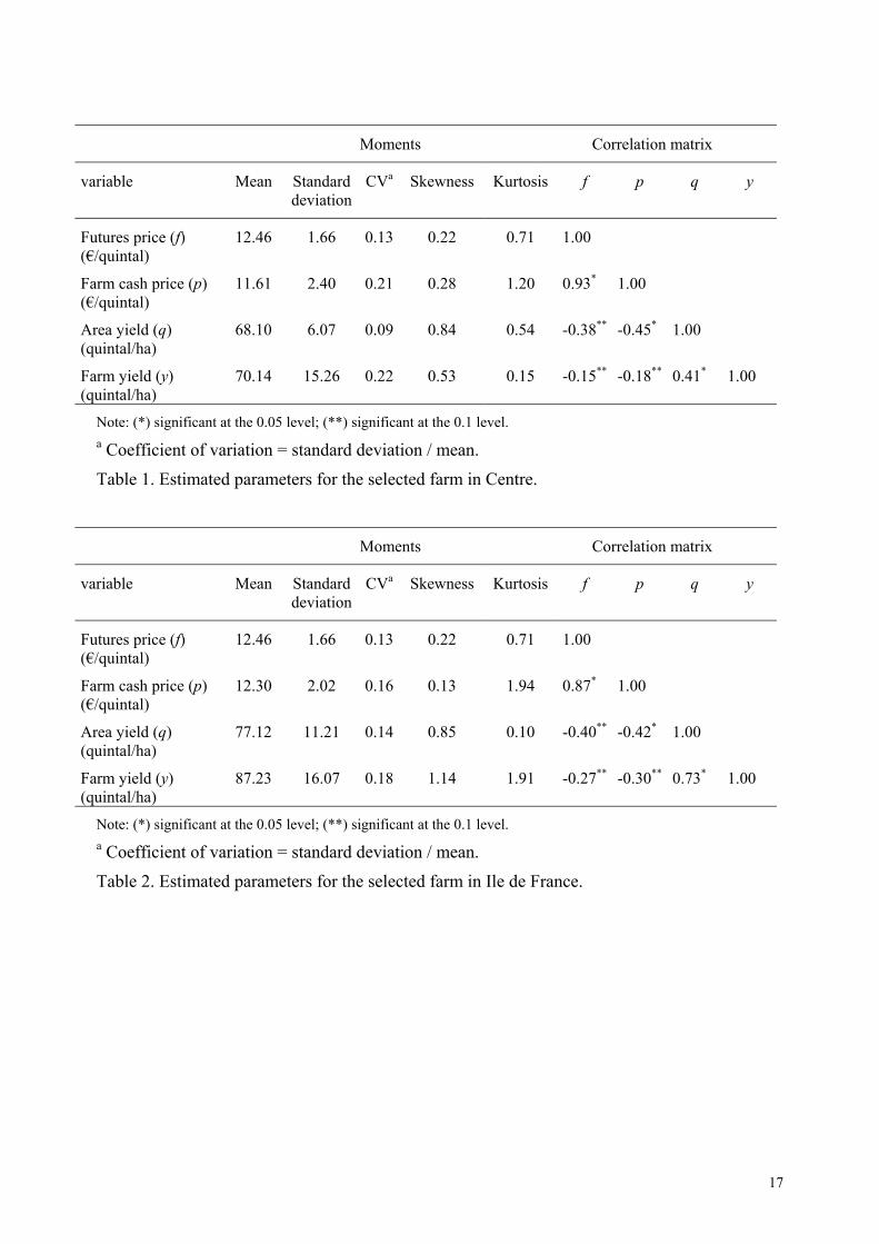
Since we focus on farms producing a single commodity (wheat), two producers were selected among farms in which the fraction of the acreage devoted to wheat is higher than 80 percent of the total acreage. Statistics for the selected farm in Center (C-farm) and in Ile de France (IdF-farm) are reported in Tables 1 and 2, respectively.10 Centre is a region with lower expected yields and lower yield variability (in terms of coefficient of variation) than Ile de France. Expected individual cash price of the C-farm is lower that of the IdF-farm, and the individual price variability of the C-farm is the highest. Skewness parameters are slightly higher than zero, indicating that the empirical probability distribution functions are slightly disymmetric. Likewise, Kurtosis parameters are slightly positive, i.e., the right-hand side tail of the distribution is heavier than the left-hand side one. The correlation between cash and futures prices is higher for the C-Farm (0.93) than for the IdF-farm (0.87), whereas individual and area yields are more correlated for the IdF-farm (0.73) than for the C-farm (0.41). The negative correlation between individual yields and prices is slightly lower (in absolute value) for futures than for individual cash, indicating the role of local factors effects on the price basis. Individual cash prices are more correlated with area yields than with individual yields.

[INSERT TABLES 1 AND 2 HERE] Concerning the C-farm, the initial wealth ( ) is set at 20000€, the acreage of wheat ( ) is 120 hectares, the production cost per hectare ( ) is 354€ and the direct subsidies per hectare (d) is 306€. In the case of the IdF-farm, these parameters are

0wc

A

000,100 =w , , and . Finally, the producer’s relative risk aversion parameter is set at

90=A=

382=c346=d 2θ in order to

represent moderate aversion toward risk. This implies that he exhibits a prudent behavior with a constant relative prudence parameter equal to 3.

Simulations of yield and price distributions and computations of optimal hedge ratios and willingness to receive measures are conducted with the CO module in GAUSS software and with EXCEL. From the 5,000 simulation runs, the mean of the individual revenue per hectare, i.e., individual cash price times individual yield, is estimated at 873€ for the C-farm and 1147€ for the IdF-farm. The coefficient of variation is equal to 27% and 20%, respectively. The fair insurance premium for the C-farm (resp. the IdF-farm) is equal to 1.07€/ha (resp. 0.37€/ha ) under IYCI, 0.12€/ha (resp. 1.13€/ha) under AYCI, 18.58€/ha (resp. 11.89€/ha) under IRI, 11.04€/ha (resp. 19.75€/ha) under ARI and 23.74€/ha (resp. 14.27€/ha) under CRC.11

4. Results and Discussion

4.1. Optimal hedging decisions

Futures and straddle hedge ratios are defined as the number of contracts per unit of expected output selected by the producer. From the hedging strategy in equation (14) and the producer’s 9 We acknowledge that Skewness and Kurtosis parameters must be interpreted cautiously because of the small size of the samples. 10 Conversion factors are: 1 hectare (ha)=2.471 acres; 1 quintal=100 kg=3.68 bushels. 11 In other words, the fair insurance premium rate, expressed in percentage of the expected revenue, for the C-farm (resp. the IdF-farm) is equal to 0.11% (resp. 0.03%) under IYCI, 0.01% (resp. 0.11%) under AYCI, 1.97% (resp. 1.01%) under IRI, 1.21 (resp. 1.90%) under ARI and 2.52% (resp. 1.22%) under CRC.

9

final wealth in equation (16), we denote the futures hedge ratio as )(FHR yAx= , the hedge ratio of the straddle at strike price Fk ×= 9.01 as ( )yAz1S1HR = , the hedge ratio of the straddle at strike price as Fk =2 ( )yAz2S2HR = and the hedge ratio of the straddle at strike price as Fk ×= 1.13 ( )yA3z=S3HR .

The beta coefficient, well-known in the Capital Asset pricing Model, measures the sensitivity of individual cash price to movements in futures prices. It is the the slope of the linear regression of individual cash on futures prices. It is equal to 1.29 for the selected farm in Centre and to 0.68 for the selected farm in Ile de France.12 If there was no production risk, the optimal unbiased futures hedge ratio would thus reduce to the beta coefficient, a well known result in the optimal hedging literature (see, for example, Benninga, Eldor and Zilcha, 1984).

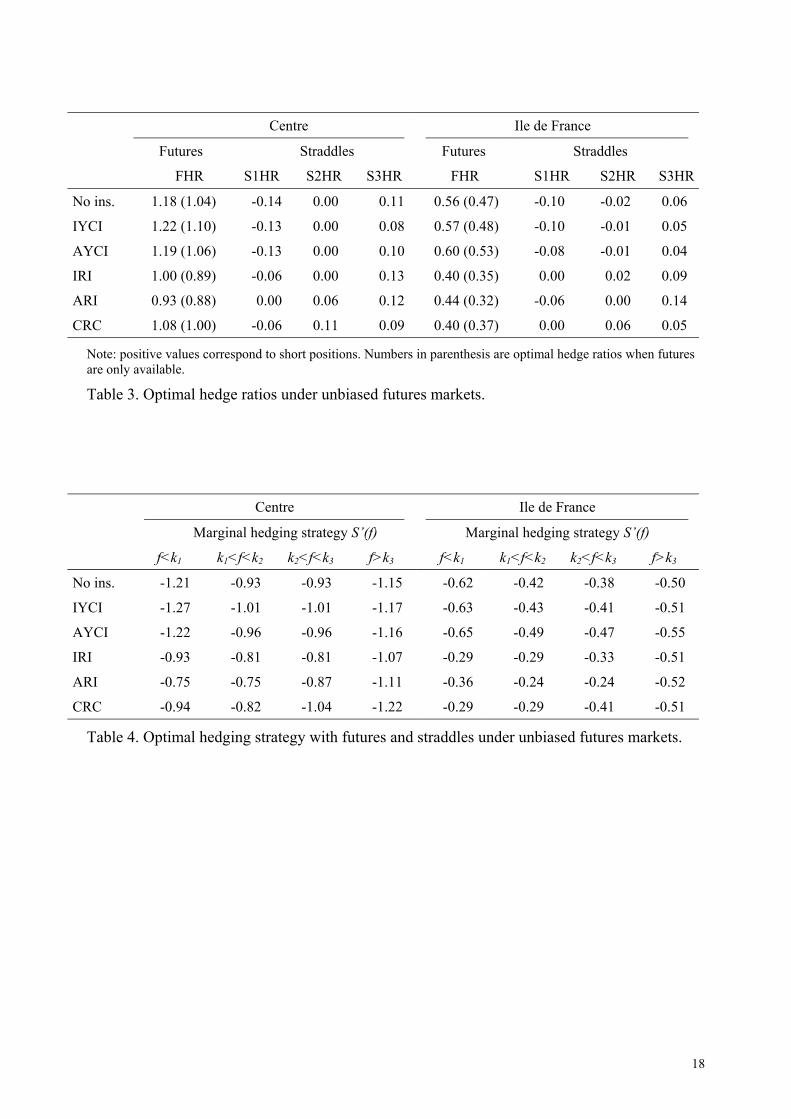
Table 3 shows the optimal hedge ratios under alternative insurance policies when futures markets are perceived as unbiased, i.e., fEF ~

= . Consider first the optimal futures hedge ratios when options are not available. They are lower than their associated beta coefficients, whatever the insurance policy, for the two selected farms. This would be due to the prudent prudent behavior of the producer who is induced to reduce his futures hedge ratio when yields are random (Mahul, 2002), and to the negative correlation between yields and prices which creates a natural hedge.13 The futures hedge ratios are lower under revenue insurance than under yield insurance because the indemnity schedule under revenue insurance offers a partial coverage against price variability. When options contracts are available, the producer would select a higher futures hedge ratio whatever the insurance policy for the two selected farms. Therefore, the availability of straddles increases the demand for futures: options and futures contracts are complementary. The optimal hedge ratio of the straddle with the lowest strike price, S1HR, is non-positive (i.e., long position) under all insurance policies for the two selected farms. In addition, S1HR is, in absolute value, higher under yield insurance than under revenue insurance. The position for the straddle at strike price k F=2 , S2HR, is close to zero, except under CRC for the two selected farms and ARI for the C-farm. Finally, the optimal hedging strategy entails selling straddles at the highest strike price k , S3HR>0, under all insurance policies for the two selected farms.

S3

[INSERT TABLE 3 HERE] The futures and straddles hedge ratios characterize the shape of the optimal hedging strategy

, as shown in equation (15). The futures hedge ratio gives the general trend of the optimal hedging strategy while the straddle hedge ratio expresses the curvature of around its strike price. The slopes of the piecewise linear hedging strategy,

SS S

( )fS ′ , are reported in Table 4. Since these values are negative, the optimal hedging strategy is a decreasing function of the realized futures price. It is not globally concave for all realized future prices, except under ARI for the selected farm in Centre. It is globally convex around the lowest strike price k under all insurance policies for the two selected farms, except under ARI for the C-farm and under CRC and IRI for the IdF-farm where it is linear. Around the intermediate strike price k , the C-farm’s optimal hedging strategy is linear, except under ARI and CRC where it is globally concave. For the IdF-farm, is globally concave around under IRI or CRC, linear under ARI and globally convex otherwise. Finally, the optimal hedging strategy is globally concave around the highest strike price under every insurance policies for the two selected farms.

1

2

S 2k

3k

[INSERT TABLE 4 HERE] 12 These regression parameters are significant at the 0.05 level. 13 If the elasticity of individual output with respect to the individual cash price would be equal to –1, then the individual gross revenue would be nonrandom and, therefore, fair insurance and hedging contracts would be useless.

10

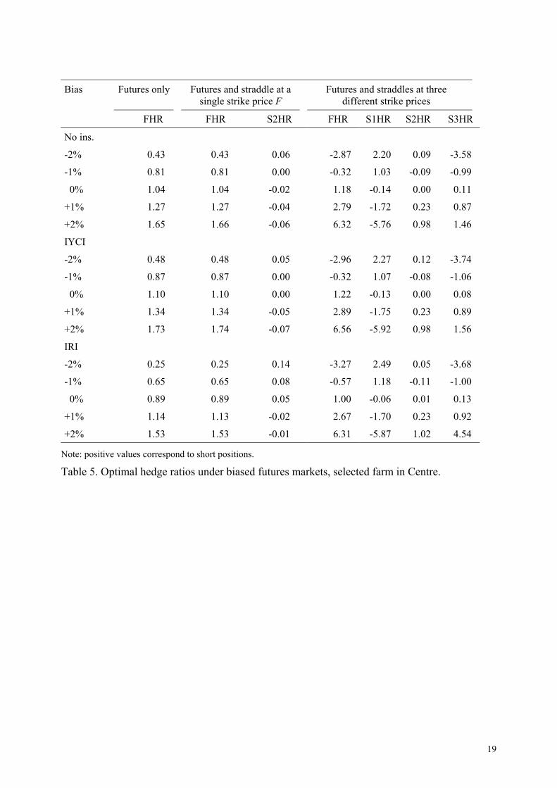
The impact of perceived bias in futures prices at harvest on optimal hedging positions is examined for the selected farm in Centre with no insurance, individual yield insurance IYCI or individual revenue insurance IRI. Optimal hedge ratios when the futures market exhibits normal backwardation (i.e., negative futures price bias), unbiasedness (i.e., no futures price bias) or contango (i.e., positive futures price bias) are reported in Table 5. Three hedging strategies are successively considered: the futures market is only available, then the straddle at a single strike price is introduced in addition to the futures contract and, finally, the futures contract and the straddles at three different strike prices are at the producer’s disposal. The hedge ratio can be broken down into two parts: a pure hedge component and a speculative component. The latter is characterized by the deviation of the ratio in biased markets from that in unbiased markets. Of course, this speculative component is null under unbiased futures markets and thus the hedge ratio is equal to the pure hedge component.

Fk =2

The optimal futures hedge ratio is first analyzed. It is noteworthy that the pure hedge component is always a short position. Contango induces the producer to select a short speculative position, whereas normal backwardation implies a long speculative position, with or without available straddles contracts, under the three insurance policies under consideration. Such a speculative behavior is consistent with the optimal hedging behavior in a futures market when production is nonrandom (see, for example, Briys, Crouhy and Schlesinger, 1993). Observe that, when straddles at three different strike prices are available, normal backwardation induces the producer to ‘go long’ in futures contracts and to take a so-called ‘Texan position’. The long speculative position is thus higher than the short pure hedge position. In addition, the speculative component of the futures hedge ratio increases with the futures bias (in either direction).14 Introducing straddles at a single strike price Fk =2 does not significantly affect the optimal futures hedge ratio. On the contrary, when straddles at three different strike prices are at the producer’s disposal, the speculative component of the future hedge ratio is quite sensible to the perceived bias in the futures price. For example, futures hedge ratio is greater than 6 under the three insurance policies when the futures price at harvest is perceived to be two percent higher than the expected futures price. The availability of straddles at three different strike prices gives the producer the opportunity to adopt a more aggressive speculative futures position. Such an attitude is increased by the absence of transaction costs.15

When straddles area only available at a single strike price, in addition to futures, the straddle ratio is not very sensitive to bias in the futures price. When straddles are three strike prices are offered to the producer, straddle ratios are quite sensitive. The optimal hedge ratio of the straddle at the highest strike price, S3HR, evolves as the futures hedge ratio: its optimal position is long (resp. short) under normal backwardation (resp. contango) and it increases with the bias (in either direction). The hedge ratio of the straddle at the lowest strike price, S1HR, acts in the opposite direction: its optimal position is short (resp. long) if normal backwardation (resp. contango) prevails in the futures market. It also increases with the bias (either direction). The position of the straddle at the intermediate strike is less sensitive to the perceived bias than the two other straddle contracts. The optimal position is short when the futures market exhibits contango while it can be either long or short under normal backwardation.

[INSERT TABLE 5 HERE]

14 This relationship is far from obvious in a theoretical viewpoint. One can easily show that when futures are only available and in the absence of basis risk, a sufficient condition for the producer to increase his short futures position as the futures price at harvest increases in that his degree of relative risk aversion is lower than unity. In other words, for a producer with a degree of relative risk aversion higher than unity, the relationship between the short futures position and the futures price at harvest may be either negative or positive. 15 We restrict our analysis to bias in futures prices, in absolute value, lower than or equal to 2 percent because greater bias would generate higher hedge ratios that are not realistic without taking into account transaction costs.

11

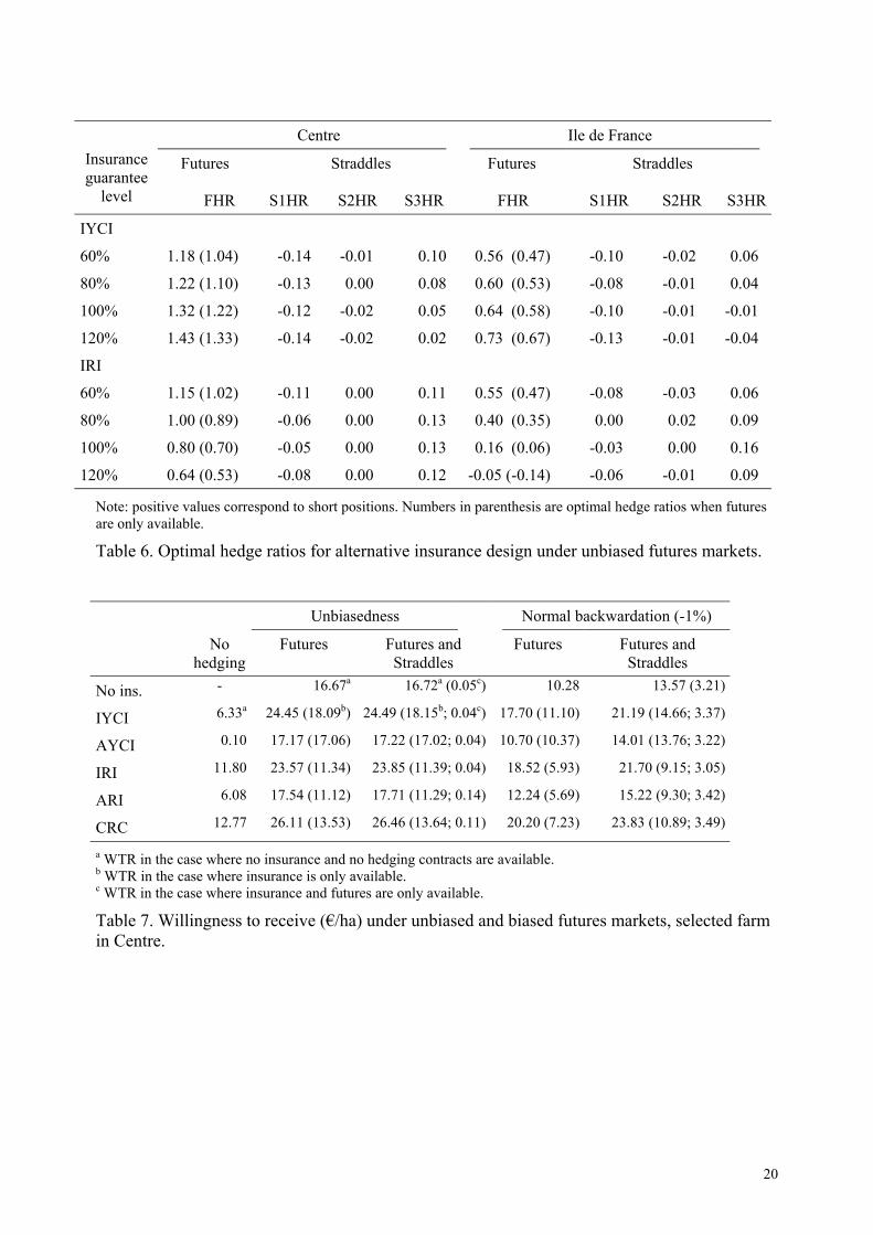
The demand for hedging against price uncertainty has be shown to depend on the insurance policy under consideration. The impact of insurance guarantee on the optimal futures and straddles positions is evaluated when the producer is endowed with individual yield insurance IYCI or individual revenue insurance IRI. Results are reported in Table 6. As the insurance guarantee increases, the optimal futures hedge ratio should increase under IYCI and decrease under IRI, with or without available straddles contracts. Such relationships are observed by Coble, Heifner and Zuniga (2000) when futures are only available. Therefore, the complementarity between futures and crop yield insurance and the substituability between futures and crop revenue insurance hold when straddles are offered to the producer. Observe that the IRI contract at 120% guarantee level induces the IdF-farm to buy futures (FHR<0). This long futures position is increased when straddles are available. This means that the slope of the first-best hedging strategy expressed in equation (6) is positive, i.e., the covariance term is positive. In all other cases, introducing straddles induces the producers to increase their short futures position. Finally, Table 6 shows that straddles positions are almost insensitive to changes in insurance guarantee levels.

[INSERT TABLE 6 HERE]

4.2. Performance of hedging instruments

The increased producer welfare from risk reduction generated by insurance policy and/or financial contracts is evaluated by a willingness to receive measure (WTR). It is calculated as the amount of sure income that must be provided to the producer in the case where risk management instruments are not available, in order to generate the same level of expected utility achieved when these risk management tools are available and efficiently used. For instance, the WTR for the revenue insurance contract i in the case where no insurance and hedging tools are available, denoted , is given by: i

1WTR

( )( ) ( )( )ii ycypEuNIycypEu 1WTR~~~~ +−=+− . (17) Performance associated to a given risk management strategy (rm1) with respect to another risk management strategy (rm2) where some instruments are not available is measured by the WTR for rm1 in the case where rm2 is at the producer’s disposal. It is important to notice that, contrary to a widespread belief (see, for example, Wang et al., 1998), there is no theoretical basis to state that the WTR for, say, the addition of futures and straddles to the portfolio where insurance is available is equal to difference between the WTR of insurance, futures and straddles in the case where no hedging tools are available, and the WTR of insurance in the case where no hedging tools are available. Formally, define and as i

2WTR i3WTR

( ) ( )( ) ( )( )ii ycypEufSNIycypEu 2WTR~~~~~ +−=++− (18) and

( ) ( )( ) ( )( )iii NIycypEufSNIycypEu 3WTR~~~~~ ++−=++− . (19)

Therefore, may be higher than, equal to, or lower than i3WTR ( )ii

12 WTRWTR − . This possible non-additivity of WTR under risk will be illustrated using our simulation results.

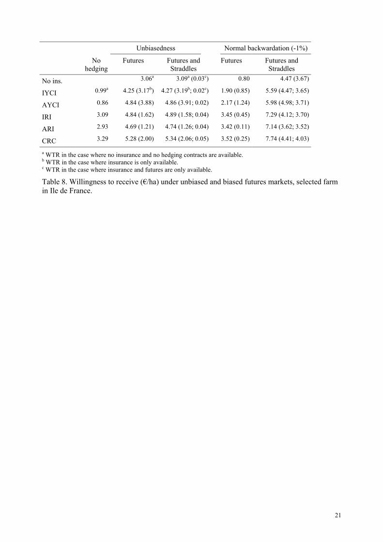
The performance of insurance and financial contracts, measured in terms of WTR, are reported in Tables 7 and 8 for the selected farm in Centre and in Ile de France, respectively. Suppose first that insurance contracts are only available. The existence of an insurance market increases the C-farm’s WTR in the range of 0.10€/ha to 12.77€/ha, and the IdF-farm’s WTR in the range of 0.86€/ha to 3.29€/ha. These positive, but sometimes low, WTR are not surprising at all because it is well-known that insurance (in which the index used in the indemnity payoff is positively correlated with the individual loss) sold at a fair price reduces the agent’s exposure to risk without reducing his expected wealth and, therefore, it increases the risk-averse agent’s

12

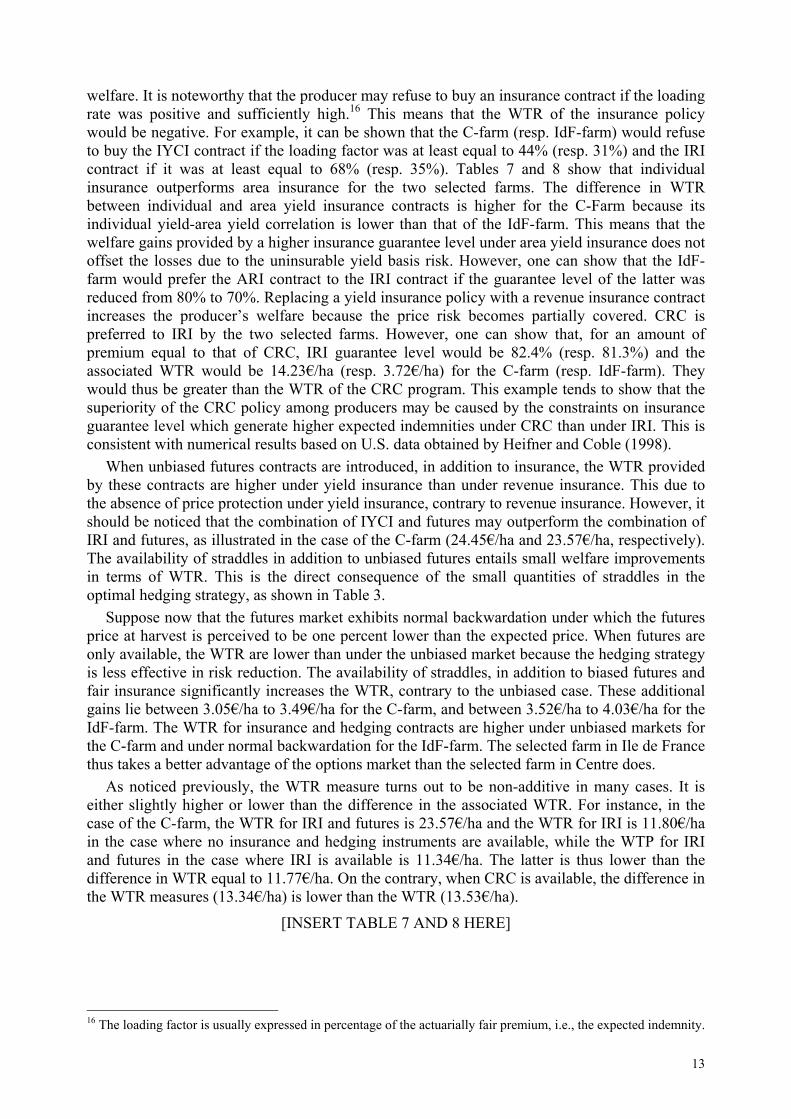
welfare. It is noteworthy that the producer may refuse to buy an insurance contract if the loading rate was positive and sufficiently high.16 This means that the WTR of the insurance policy would be negative. For example, it can be shown that the C-farm (resp. IdF-farm) would refuse to buy the IYCI contract if the loading factor was at least equal to 44% (resp. 31%) and the IRI contract if it was at least equal to 68% (resp. 35%). Tables 7 and 8 show that individual insurance outperforms area insurance for the two selected farms. The difference in WTR between individual and area yield insurance contracts is higher for the C-Farm because its individual yield-area yield correlation is lower than that of the IdF-farm. This means that the welfare gains provided by a higher insurance guarantee level under area yield insurance does not offset the losses due to the uninsurable yield basis risk. However, one can show that the IdF-farm would prefer the ARI contract to the IRI contract if the guarantee level of the latter was reduced from 80% to 70%. Replacing a yield insurance policy with a revenue insurance contract increases the producer’s welfare because the price risk becomes partially covered. CRC is preferred to IRI by the two selected farms. However, one can show that, for an amount of premium equal to that of CRC, IRI guarantee level would be 82.4% (resp. 81.3%) and the associated WTR would be 14.23€/ha (resp. 3.72€/ha) for the C-farm (resp. IdF-farm). They would thus be greater than the WTR of the CRC program. This example tends to show that the superiority of the CRC policy among producers may be caused by the constraints on insurance guarantee level which generate higher expected indemnities under CRC than under IRI. This is consistent with numerical results based on U.S. data obtained by Heifner and Coble (1998).

When unbiased futures contracts are introduced, in addition to insurance, the WTR provided by these contracts are higher under yield insurance than under revenue insurance. This due to the absence of price protection under yield insurance, contrary to revenue insurance. However, it should be noticed that the combination of IYCI and futures may outperform the combination of IRI and futures, as illustrated in the case of the C-farm (24.45€/ha and 23.57€/ha, respectively). The availability of straddles in addition to unbiased futures entails small welfare improvements in terms of WTR. This is the direct consequence of the small quantities of straddles in the optimal hedging strategy, as shown in Table 3.

Suppose now that the futures market exhibits normal backwardation under which the futures price at harvest is perceived to be one percent lower than the expected price. When futures are only available, the WTR are lower than under the unbiased market because the hedging strategy is less effective in risk reduction. The availability of straddles, in addition to biased futures and fair insurance significantly increases the WTR, contrary to the unbiased case. These additional gains lie between 3.05€/ha to 3.49€/ha for the C-farm, and between 3.52€/ha to 4.03€/ha for the IdF-farm. The WTR for insurance and hedging contracts are higher under unbiased markets for the C-farm and under normal backwardation for the IdF-farm. The selected farm in Ile de France thus takes a better advantage of the options market than the selected farm in Centre does.

As noticed previously, the WTR measure turns out to be non-additive in many cases. It is either slightly higher or lower than the difference in the associated WTR. For instance, in the case of the C-farm, the WTR for IRI and futures is 23.57€/ha and the WTR for IRI is 11.80€/ha in the case where no insurance and hedging instruments are available, while the WTP for IRI and futures in the case where IRI is available is 11.34€/ha. The latter is thus lower than the difference in WTR equal to 11.77€/ha. On the contrary, when CRC is available, the difference in the WTR measures (13.34€/ha) is lower than the WTR (13.53€/ha).

[INSERT TABLE 7 AND 8 HERE]

16 The loading factor is usually expressed in percentage of the actuarially fair premium, i.e., the expected indemnity.

13

5. Conclusion

This paper provides an analysis on the optimal hedging demand against price risk with futures and options when crop yield and revenue insurance are also available. The first-best hedging strategy against price risk is shown to be altered by the presence of crop yield or revenue insurance policies. However, introducing a crop yield insurance policy does not affect the form of the optimal hedging contract for a producer with a quadratic utility function. Numerical simulations using French individual data are conducted to investigate the optimal hedging demand with futures and options. They stress the complementarity between futures and options contracts by showing that the introduction of options would induce the producers to sell more futures contracts. The demand for straddles would be rather limited when the futures market is unbiased, but it would significantly increase as the futures market exhibits normal backwardation or contango. The availability of straddles would induce the producer to adopt a more aggressive speculative position on the futures market. Revenue insurance tends to result in lower demand for futures contracts, with or without available straddles, than yield insurance. The futures hedge ratio would increase with the yield insurance guarantee. On the contrary, it would decrease as the revenue insurance guarantee increases. This means that the demand for futures contracts would be complement with crop yield insurance and substitute with crop revenue insurance. Straddles positions are almost insensitive to changes in insurance guarantee levels.

The availability of unbiased futures contracts would significantly increase the producer’s welfare, in terms of willingness to receive. It would be reduced if normal backwardation prevails on the futures market. Straddles are shown to be weakly performing when futures markets are unbiased, while they are more performing when the futures market exhibits normal backwardation or contango.

These findings should be tempered, however, by the fact that the size of our sample is small, only two individual farms have been considered and transaction costs have been ignored. In addition, they may be sensitive to the specific assumptions used to implement the numerical model. Consequently, these results must be viewed as exploratory. Nevertheless, they provide interesting results on the demand for hedging against price risk with both futures contracts and straddles at three different strike prices. Further research would examine other crops and regions, and would introduce transaction costs.

14

References Barnett, B.J. (2001). The U.S. federal crop insurance program. Canadian Journal of

Agricultural Economics 48: 539-551. Benninga, S., Eldor, R., & Zilcha, I. (1984). The optimal hedge ratio in unbiased futures

markets. The Journal of Futures Markets 4: 155-159. Coble, K.H., Heifner, R.G. and Zuniga M. (2000). Implications of crop yield and revenue

insurance for producer hedging. Journal of Agricultural and Resource Economics 25(2): 432-453.

Fleishman A.I. (1978). A method for simulating non-normal distributions. Psycometrika 43(4): 521-532.

Froot, K., Scharfstein D. and Stein, J. (1993). Risk management: coordinating corporate investment and financing decisions. Journal of Finance 48: 1629-1658.

Greenwald, B.C. and Stiglitz, J.E. (1993). Financial market imperfections and business cycles. Quarterly Journal of Economics 108: 77-114.

Kimball, M.S. 1990. Precautionary savings in the small and in the large. Econometrica 58(1): 53-73.

Losq, E. (1982). Hedging with price and output uncertainty. Economics Letters 10: 65-70. Mahul O. (1999). Optimum area yield crop insurance. American Journal of Agricultural

Economics 81(1): 75-82. Mahul, O. (2000). Optimum crop insurance under joint yield and price risk. Journal of Risk and

Insurance 67: 109-122. Mahul, O. (2002). Optimal hedging in futures and options markets. Journal of Futures Markets

22(1): 59-72. Mahul, O. and Vermersch D. (2000). Hedging crop risks with insurance futures and options.

European Review of Agricultural Economics 27: 49-58. McKinnon, R.I. (1967). Futures markets, buffer stocks, income stability for primary producers.

Journal of Political Economy 75: 844-861. Miranda, M. (1991). Area-yield crop insurance reconsidered. American Journal of Agricultural

Economics 73(2): 233-42. Moschini, H. and Lapan H. (1995). The hedging role of options and futures under joint, price,

basis, and production risk. International Economic Review 36(4): 1025-1049. Rolfo, J. (1980). Optimal hedging under price quantity uncertainty: the case of cocoa producer.

Journal of Political Economy 88: 100-116. Skees, J., Black, J.R. and Barnett, B.J. (1997). Designing and rating an area yield crop insurance

contract. American Journal of Agricultural Economics 79(2): 233-42. Smith, C.W. and Stulz, R. (1985). The determinants of firms’ hedging policies. Journal of

Financial and Quantitative Analysis 20: 391-405. Vale, C.D. and Maurelli, V.A. (1983). Simulating multivariate nonnormal distributions.

Psycometrika 48(3): 465-471. Vercammen, J. (2000). Constrained efficient contracts for area yield crop insurance. American

Journal of Agricultural Economics 82(4): 856-864. Wang, H.H., Hanson, S.D., Myers, R.J. and Black, J.R. (1998). The effects of crop yield

insurance designs on farmer participation ad welfare, American Journal of Agricultural Economics 80(4): 806-820.

15

Appendix

First-best hedging contract under revenue insurance

Since the marginal payoff function appears neither in the objective function nor in the constraints, the maximization problem (1) with final wealth (3) can be solved by using Kuhn-Tucker conditions for ( )pJ for all p . The first-order condition with respect to is ( )pJ

( ) ( ) ( )( ) ( ) 0~~ =−Φ+−++−′ µλpPpJypNIycypuE for all p , (A1)

where µ and are the Lagrangian multipliers associated with the premium constraint and the non-negative indemnity constraint respectively, with

( )pΦ

( ) ( )≥

>=Φ

otherwise.00 if0 pJ

p (A2)

For all , (A1) can be rewritten as ( ) 0: =pJp

( ) ( ) ( )( 0)~~ ≤−−+−′= µλPypNIycypuEpK , (A3)

and its first derivative is

( ) ( )( ) ( ) ( )([ ]PypNIycypuypINypEpK )−+−′′′+=′ ~~~1~ . (A4)

If the producer is not over-indemnified when a loss occurs, i.e., ( ) 1−≥′ zIN with a strict inequality at some , and under risk aversion, z K is decreasing with p . This implies that the optimal hedging contract is of the form:

( )=

<>otherwise.0

ˆ if0 pppJ (A5)

For all , we have ( ) 0: >pJp

( ) ( ) ( )( ) µλ=−++−′ PpJypNIycypuE ~~ . (A6)

Differentiating (A6) with respect to p yields

( )( ) ( )[ ] ( ) ( ) ( )( ){ } 0~~~1~ =−++−′′′+′+ PpJypNIycypupJypINyE . (A7)

Rearranging the terms gives equation (6).

16

Moments Correlation matrix

variable Mean Standard deviation

CVa Skewness Kurtosis f p q y

Futures price (f) (€/quintal)

12.46 1.66 0.13 0.22 0.71 1.00

Farm cash price (p) (€/quintal)

11.61 2.40 0.21 0.28 1.20 0.93* 1.00

Area yield (q) (quintal/ha)

68.10 6.07 0.09 0.84 0.54 -0.38** -0.45* 1.00

Farm yield (y) (quintal/ha)

70.14 15.26 0.22 0.53 0.15 -0.15** -0.18** 0.41* 1.00

Note: (*) significant at the 0.05 level; (**) significant at the 0.1 level. a Coefficient of variation = standard deviation / mean.

Table 1. Estimated parameters for the selected farm in Centre.

Moments Correlation matrix

variable Mean Standard deviation

CVa Skewness Kurtosis f p q y

Futures price (f) (€/quintal)

12.46 1.66 0.13 0.22 0.71 1.00

Farm cash price (p) (€/quintal)

12.30 2.02 0.16 0.13 1.94 0.87* 1.00

Area yield (q) (quintal/ha)

77.12 11.21 0.14 0.85 0.10 -0.40** -0.42* 1.00

Farm yield (y) (quintal/ha)

87.23 16.07 0.18 1.14 1.91 -0.27** -0.30** 0.73* 1.00

Note: (*) significant at the 0.05 level; (**) significant at the 0.1 level. a Coefficient of variation = standard deviation / mean.

Table 2. Estimated parameters for the selected farm in Ile de France.

17

Centre Ile de France

Futures Straddles Futures Straddles

FHR S1HR S2HR S3HR FHR S1HR S2HR S3HR

No ins. 1.18 (1.04) -0.14 0.00 0.11 0.56 (0.47) -0.10 -0.02 0.06

IYCI 1.22 (1.10) -0.13 0.00 0.08 0.57 (0.48) -0.10 -0.01 0.05

AYCI 1.19 (1.06) -0.13 0.00 0.10 0.60 (0.53) -0.08 -0.01 0.04

IRI 1.00 (0.89) -0.06 0.00 0.13 0.40 (0.35) 0.00 0.02 0.09

ARI 0.93 (0.88) 0.00 0.06 0.12 0.44 (0.32) -0.06 0.00 0.14

CRC 1.08 (1.00) -0.06 0.11 0.09 0.40 (0.37) 0.00 0.06 0.05

Note: positive values correspond to short positions. Numbers in parenthesis are optimal hedge ratios when futures are only available.

Table 3. Optimal hedge ratios under unbiased futures markets.

Centre Ile de France

Marginal hedging strategy S’(f) Marginal hedging strategy S’(f)

f<k1 k1<f<k2 k2<f<k3 f>k3 f<k1 k1<f<k2 k2<f<k3 f>k3

No ins. -1.21 -0.93 -0.93 -1.15 -0.62 -0.42 -0.38 -0.50

IYCI -1.27 -1.01 -1.01 -1.17 -0.63 -0.43 -0.41 -0.51

AYCI -1.22 -0.96 -0.96 -1.16 -0.65 -0.49 -0.47 -0.55

IRI -0.93 -0.81 -0.81 -1.07 -0.29 -0.29 -0.33 -0.51

ARI -0.75 -0.75 -0.87 -1.11 -0.36 -0.24 -0.24 -0.52

CRC -0.94 -0.82 -1.04 -1.22 -0.29 -0.29 -0.41 -0.51

Table 4. Optimal hedging strategy with futures and straddles under unbiased futures markets.

18

Bias Futures only Futures and straddle at a single strike price F

Futures and straddles at three different strike prices

FHR FHR S2HR FHR S1HR S2HR S3HR

No ins.

-2% 0.43 0.43 0.06 -2.87 2.20 0.09 -3.58

-1% 0.81 0.81 0.00 -0.32 1.03 -0.09 -0.99

0% 1.04 1.04 -0.02 1.18 -0.14 0.00 0.11

+1% 1.27 1.27 -0.04 2.79 -1.72 0.23 0.87

+2% 1.65 1.66 -0.06 6.32 -5.76 0.98 1.46

IYCI

-2% 0.48 0.48 0.05 -2.96 2.27 0.12 -3.74

-1% 0.87 0.87 0.00 -0.32 1.07 -0.08 -1.06

0% 1.10 1.10 0.00 1.22 -0.13 0.00 0.08

+1% 1.34 1.34 -0.05 2.89 -1.75 0.23 0.89

+2% 1.73 1.74 -0.07 6.56 -5.92 0.98 1.56

IRI

-2% 0.25 0.25 0.14 -3.27 2.49 0.05 -3.68

-1% 0.65 0.65 0.08 -0.57 1.18 -0.11 -1.00

0% 0.89 0.89 0.05 1.00 -0.06 0.01 0.13

+1% 1.14 1.13 -0.02 2.67 -1.70 0.23 0.92

+2% 1.53 1.53 -0.01 6.31 -5.87 1.02 4.54

Note: positive values correspond to short positions.

Table 5. Optimal hedge ratios under biased futures markets, selected farm in Centre.

19

Centre Ile de France Insurance guarantee

Futures Straddles Futures Straddles

level FHR S1HR S2HR S3HR FHR S1HR S2HR S3HR

IYCI

60% 1.18 (1.04) -0.14 -0.01 0.10 0.56 (0.47) -0.10 -0.02 0.06

80% 1.22 (1.10) -0.13 0.00 0.08 0.60 (0.53) -0.08 -0.01 0.04

100% 1.32 (1.22) -0.12 -0.02 0.05 0.64 (0.58) -0.10 -0.01 -0.01

120% 1.43 (1.33) -0.14 -0.02 0.02 0.73 (0.67) -0.13 -0.01 -0.04

IRI

60% 1.15 (1.02) -0.11 0.00 0.11 0.55 (0.47) -0.08 -0.03 0.06

80% 1.00 (0.89) -0.06 0.00 0.13 0.40 (0.35) 0.00 0.02 0.09

100% 0.80 (0.70) -0.05 0.00 0.13 0.16 (0.06) -0.03 0.00 0.16

120% 0.64 (0.53) -0.08 0.00 0.12 -0.05 (-0.14) -0.06 -0.01 0.09

Note: positive values correspond to short positions. Numbers in parenthesis are optimal hedge ratios when futures are only available.

Table 6. Optimal hedge ratios for alternative insurance design under unbiased futures markets.

Unbiasedness Normal backwardation (-1%)

No hedging

Futures Futures and Straddles

Futures Futures and Straddles

No ins. - 16.67a 16.72a (0.05c) 10.28 13.57 (3.21)

IYCI 6.33a 24.45 (18.09b) 24.49 (18.15b; 0.04c) 17.70 (11.10) 21.19 (14.66; 3.37)

AYCI 0.10 17.17 (17.06) 17.22 (17.02; 0.04) 10.70 (10.37) 14.01 (13.76; 3.22)

IRI 11.80 23.57 (11.34) 23.85 (11.39; 0.04) 18.52 (5.93) 21.70 (9.15; 3.05)

ARI 6.08 17.54 (11.12) 17.71 (11.29; 0.14) 12.24 (5.69) 15.22 (9.30; 3.42)

CRC 12.77 26.11 (13.53) 26.46 (13.64; 0.11) 20.20 (7.23) 23.83 (10.89; 3.49)

a WTR in the case where no insurance and no hedging contracts are available. b WTR in the case where insurance is only available. c WTR in the case where insurance and futures are only available.

Table 7. Willingness to receive (€/ha) under unbiased and biased futures markets, selected farm in Centre.

20

Unbiasedness Normal backwardation (-1%)

No hedging

Futures Futures and Straddles

Futures Futures and Straddles

No ins. 3.06a 3.09a (0.03c) 0.80 4.47 (3.67)

IYCI 0.99a 4.25 (3.17b) 4.27 (3.19b; 0.02c) 1.90 (0.85) 5.59 (4.47; 3.65)

AYCI 0.86 4.84 (3.88) 4.86 (3.91; 0.02) 2.17 (1.24) 5.98 (4.98; 3.71)

IRI 3.09 4.84 (1.62) 4.89 (1.58; 0.04) 3.45 (0.45) 7.29 (4.12; 3.70)

ARI 2.93 4.69 (1.21) 4.74 (1.26; 0.04) 3.42 (0.11) 7.14 (3.62; 3.52)

CRC 3.29 5.28 (2.00) 5.34 (2.06; 0.05) 3.52 (0.25) 7.74 (4.41; 4.03)

a WTR in the case where no insurance and no hedging contracts are available. b WTR in the case where insurance is only available. c WTR in the case where insurance and futures are only available.

Table 8. Willingness to receive (€/ha) under unbiased and biased futures markets, selected farm in Ile de France.

21