Hedge ratios for short and leveraged ETFs Review of Economics – 1st Volume - 2011 Revista...

Atlantic Review of Economics – 1st Volume - 2011

Revista Atlántica de Economía – Volumen 1 - 2011 1

Hedge ratios for short and leveraged ETFs

Leo Schubert1 Constance University of Applied Sciences

1 [email protected]


Revista Atlántica de Economía – Volumen 1 - 2011

2

Abstract Exchange-traded funds (ETFs) exist for stock, bond and commodity markets. In most cases

the underlying feature of an ETF is an index. Fund management today uses the active and

the passive way to construct a portfolio. ETFs can be used for passive portfolio

management, for which ETFs with positive leverage factors are preferred. In the frame of an

active portfolio management the ETFs with negative leverage factors can also be applied for

the hedge or cross hedge of a portfolio. These hedging possibilities will be analysed in this

paper. Short ETFs exist with different leverage factors. In Europe, the leverage factors 1 (e.g.

ShortDAX ETF) and 2 (e.g. DJ STOXX 600 Double Short) are offered while in the financial

markets of the United States factors from 1 to 4 can be found. To investigate the effect of the

different leverage factors and other parameters Monte Carlo simulation was used. The

results show for example that higher leverage factors achieve higher profits as well as

losses. In the case that a bearish market is supposed, minimizing the variance of the hedge

seems not to obtain better hedging results, due to a very skewed return distribution of the

hedge. The risk measure target-shortfall probability confirms the use of the standard hedge

weightings, which depend only on the leverage factor. This characteristic remains when a

portfolio has to be hedged instead of the underlying index of the short ETF. For portfolios that

have a low correlation with the index return high leverage factors should not be used for

hedging, due to the higher volatility and target-shortfall probability. Resumen

Los fondos negociables en el mercado o EFTs (Exchange Traded Funds) existen en los

mercados de valores – bonos – y de mercancías. En la mayoría de los casos tras un EFT

hay un índice. La gestión actual de fondos utiliza formas activas y pasivas para construir

una cartera de valores o portfolio. De esa forma, se opta por EFTs con factores de

influencia positiva. En el marco de un portfolio activo también se pueden aplicar EFTs con

factores de influencia negativa para la cobertura de una cartera de acciones. En este

documento se analizarán estas posibilidades de cobertura. Existen EFTs con diferentes

factores de cobertura. En Europa se ofrecen los factores de cobertura 1 (por ejemplo,

ShortDAX ETF) y 2 (por ejemplo, DJ STOXX 600 Double Short), mientras que en los

mercados financieros de EEUU encontramos factores del 1 al 4. Para analizar el efecto de

los diferenteS factores de cobertura, así como de otros parámetros, utilizamos la Simulación

Monte Carlo. Los resultados muestran, por ejemplo, que con factores con mayor cobertura



3

se obtiene tanto mayores beneficios como pérdidas. En el supuesto de un mercado con

tendencia a la baja no parece que se minimice la variedad de la cobertura hasta que se

consiguen mejores resultados, debido a una distribución muy sesgada de los rendimientos.

Esa característica se mantiene también en el caso de que un portfolio tenga que ser

cubierto o protegido, en lugar de utilizar el índice de un ETF short o reducido. Para aquellos

portfolios con una baja correlación con los beneficios del índice, no deberían utilizarse

factores de elevada cobertura, debido a la mayor volatilidad y probabilidad de déficit en los

objetivos.

JEL-Classification-System: G11, G24, G32, C15 Key-Words: Portfolio Optimization, Hedging, Cross Hedge, Insurance and Immunization of Portfolios, Short Leveraged Exchange-Traded Funds (ETFs), Mean–Variance, Target-Shortfall Probability, Monte Carlo Simulation



4

1. Introduction

An exchange-traded fund (ETF) is a reconstructed index. If no index exists in some regions or

sectors a portfolio whose structure is publicized can be the underlying feature of the ETF, too. These

funds are traded every day at the exchange boards. Concerning volatility, an ETF can be denoted as

being safer than a single stock of these markets. While a (long) ETF produces returns like the index or

the underlying portfolio, short ETFs offer inverse returns. If an index loses 5% within one day, the short

ETF with this underlying index would rise by 5%. A double short ETF would rise by 10% and a triple

short ETF by 15% and so on. As described below, the rising of the short ETFs can be a little higher

due to the payment of interest. Furthermore, a tracking error and a small management fee must be

taken into consideration.

The reverse character of the short ETFs offers the possibility to apply short ETFs to hedging. The

classic hedging instruments like short future and options produce specific results. A perfect hedge with

a short future has a fixed return, which covers the cost of carry. There remains no chance to

participate in profits when the prices of the stocks of the portfolio are rising. However, the value of the

hedge would not be reduced if the prices are falling. In the case that the underlying index of the short

future and the portfolio are not identical, an optimal hedge ratio must be computed (cross hedge). The

perfect hedge can be denoted as immunization as the value of the hedge will not change when the

prices in the market change. Options offer the possibility to construct portfolio insurance. In the case of

the “protected put buying”, losses do exist – but they are limited. The portfolio insurance does not

exclude earning profits when stock prices are rising.

Using a short ETF for hedging is different in some ways from hedging with the derivative

instruments futures or puts:

• The short ETF is not only a right that can be bought – it is an investment in the sense that

more capital is needed. To reduce the capital, higher leverage factors can be used.

• Short ETFs do not have a duration like futures or puts, which need new contracts to roll on

the hedging after some time.

• Dependent on the hedging period, short ETFs can offer a kind of immunization (for short

time intervals T) and will change to a kind of insurance (for long periods T).2 The strategy

is neither bullish nor bearish; it is more a volatility-oriented strategy.3 This changing

character is illustrated in Figure 1, in which an index is hedged by a short ETF. Depending

on the time interval T of the hedge, the function of the short ETF and thus the hedge result

changes. As the short ETF pays additional interest i, the value of the short ETF in Figure 1

is placed a little higher than the value of the index when its profit is zero. The loss in the

2 In general hedging inverse ETFs reduce the volatility, which was demonstrated by Hill, J. and Teller, S. (2010). They rebalanced the hedge of the S&P 500 by short and leveraged ETFs in a 7-month time interval. 3 See Michalik Th., Schubert L. (2009).



5

case of insurance depends mainly on T, the leverage factor λ and the volatility σ of the

index return. The function of a short ETF will be presented with the equation (2-3) in the

following chapter.

immunization

index value

hedge

Hedge-ETF-2.dsf 0611

insurance

short ETFT=1 T>1 index

T=1

T>1

profit

Figure 1: Hedging with short and leveraged ETFs: immunization or insurance

To investigate the effect of the different ETFs while hedging or cross hedging a portfolio of stocks

(or an index), Monte Carlo simulation is used. Another question of hedging was considered by

Alexander C. and Barbosa A., who looked for possibilities to hedge a portfolio of ETFs using future

contracts.4

In the following chapter, the Monte Carlo simulation of asset values and their short and leveraged

ETFs will be described. This approach was preferred as the use of empirical data often has the

disadvantage that the data are restricted to particular types of ETFs,5 e.g. in Germany, where until

2009 only short ETFs (leverage factor 1) were offered. The third chapter will depict the quality of the

determined values. The effects of hedging with short and leveraged ETFs will be shown in chapter 4.

2. Monte Carlo simulation of short and leveraged ETFs

To gain some insights into the value of a short ETF, the prices of the underlying index were

generated by Monte Carlo simulation. By this simulation a discrete “random walk”6 was created for

the index. The price development of the index depends on the annual expected return value µ and the

(continuous compounded) volatility σ. For one day, the expected return is µ/360 and respectively for

the volatility 360/σ . For the simulation it is supposed that every day the stock prices are fixed at the

exchange boards. Therefore, every day the price of the short ETF can change and has to be

computed, too. The return rt for day t = 1, …, T is simulated by yt, a realization of the stochastic

4 Alexander C., Barbosa A. (2007). 5 Michalik Th., Schubert L. (2009). 6 Deutsch H. P. (2004), pp. 26–34.



6

variable Y, which is standard normal distributed. The constructed value rt is a realization of a

stochastic variable R ∼ N(µ/360, σ/3600.5):

tt y360/360/r ⋅σ+µ= with Y ∼ N(0,1). (2-1) The value I0 of the index moves within one day (t=1) to

tr1tt eII −= and respectively tr

01 eII = . (2-2) The stochastic values of rt determine the path of the price of the index within T days: I0, I1, ..., IT.

To compute the price of the short ETF, the ratios I1/I0 … IT/IT-1 were used (see (2-3)). The simulation

uses a constant interest rate i=2% p.a. and respectively 2%/360 per day. To estimate the value St of

the short ETF, the value of the last day St-1 and the leverage factor λ must be taken into consideration.

As the formula for the computation of the value of short ETFs only negative leverage factors are used;

the sign of the factor is ignored in this paper (short ETF: λ=1, double short ETF: λ=2 etc.):

⎟⎠⎞

⎜⎝⎛⋅⋅++⎟⎟

⎠

⎞⎜⎜⎝

⎛⋅−+⋅= −

− 360iS)1(λ

IIλ)1(λSS 1t

1t

t1t-t . (2-3)

Leverage Term Interest Term

After T days, the prices IT and ST are determined by equations (2-1) to (2-3). Different time jumps

for fixing the prices over the weekend etc. were ignored by the supposition that the prices of the index

and the short ETF are fixed every day.

The computation for T days was repeated 10 million times to obtain the examples depicted below

in chapters 3 and 4. For the simulation the programming language Delphi 4.0 was used. The creation

of the random numbers was performed by the RandG(0,1) function of the unit “Math”.

The results of the simulation of IT and the simultaneously determined ST by equation (2-3) were

used to compute the hedge of the index by short ETF HT=IT+ST. If this hedge should have minimal

variance, the weightings xI for the part of the budget invested in t=0 in the index and xS in the short

ETF were determined by the cross-hedge equation:7

)r,rcov(2ss)r,rcov(sx

SI2

S2

I

SI2

SI

⋅−+−

= and xS=1-xI. (2-4)

In the case of a hedge for one day (T=1), a perfect hedge is possible if the weightings

1xI +λ

λ= and

11xS +λ

= (2-5)

are used.8 This standard hedge applied for one day offers an immunization of the index value. For

short ETFs (λ=1) the weightings are xI=1/2 and xS=1/2 and for double short ETFs (λ=2) xI=2/3 and

7 See e.g. Grundmann W., Luderer B. (2003), p. 146. 8 Proof: see appendix A1.



7

xS=1/3. Higher leverage factors reduce the amount for the hedging instrument. For λ=4 the weighting

is xS=1/5, which means that only 20% of the budget has to be invested in the leveraged ETF.

The cross-hedge function (2-4) can be used when T>1, if doubts exist that the standard hedge

weightings do not minimize the risk. Then the weightings can deviate from the standard hedge

weightings (2-5) dependent on the supposed development of the index prices and respectively the

annual continuous compounded mean return µ and the volatility σ. Furthermore, the time interval T will

be considered and analysed in a chapter below. Table A3 in appendix A3 shows the results of the

variation of the parameters µ and λ. These results contain information about the weighting of xI and xS

for the “minimal variance hedge” (MVH), the expected return rI=(IT/I0-1) of the index and rS of the short

ETF after T days, the correlation corr of rI and rS and the variances of these values sI2 and sS

2. The

covariance of the cross-hedge equation (2-4) can be determined by the function cov(rI,rS)=corr·sI·sS.

With this information the complete efficient frontier of the mix of an index with a short ETF can be

computed.

Instead of an index, usually an asset or a portfolio has to be hedged. Therefore, the simulation of

the path of the index prices and the determination of the value of the short ETF must be expanded to

the simulation of the path of a portfolio. The returns of this portfolio and the index normally have a

correlation ρ<1. For the simulation of the index and the ρ-correlated portfolio, the formula

t2

ttP y'ρ1yρy ⋅−+⋅= (2-6)

was applied to obtain random numbers that generate ρ-correlated returns.9 The variable yt is a

realization of a stochastic variable Y, as described in (2-1). The value y’t signifies a realization of an

analogously defined stochastic variable Y’. The result of equation (2-6) is the realization ytP of a

stochastic variable YP, which has a correlation ρ with variable Y. The values ytP (t=1, …, T) are used to

construct the return of the portfolio and yt for the return of the index. As the variables Y and Y’ have an

expected value of 0 and variance of 1, the variable YP will have these parameters, too (see appendix

(A2-2)). With equation (2-1) and the stochastic variables Y and YP the returns of the index and the

portfolio can be computed. The path of the value of the portfolio P0, …, PT has to be computed

analogously to equation (2-2).

According to the well-known relationship10

P

P σσ

⋅ρ=β (2-7)

the βP value of a portfolio can be designed by the selection of the standard deviation σP of the

portfolio. For equal standard deviations σ=σP the simulation will generate a portfolio with low

9 Proof: see appendix A2. 10 See e.g. Bamberg, G., Baur, F. (1996), p. 44.



8

systematic risk, as βP=ρ with (ρ≤1). Furthermore, the αP value of the portfolio using equation (2-7)

would be:

µ⋅σσ

⋅ρ⋅µ=αP

PP . (2-8)

Tables A4-1 and A4-2 in appendix A4 show a different MVH from the parameters ρ=0.95, 0.90,

0.85, 0.80, 0.75. Now, instead of rI and sI2, the tables contain the expected return of the portfolio

rP=(PT/P0-1) and the variance sP2 of these portfolio returns for a given time interval T and leverage

factor λ. As above, the completely efficient frontier of the mix of a portfolio and a short ETF can be

computed by the information in these tables.

3. Quality of the Monte Carlo simulation

As the random walk of a path t = 0, …, T produces index prices IT that are lognormal distributed,

the expected mean11 E(IT) must be

360T

20T

2

eI)I(E⋅⎟⎟

⎠

⎞

⎜⎜

⎝

⎛ σ+µ

⋅= and the variance (3-1)

( ))1e(eI)I(Var 360

T360T2

0T

22

−⋅⋅=⋅σ⋅σ+µ⋅

. (3-2) A good simulation should generate good estimations of the expected parameters: E(IT) ≈ I0 ·(1+ rI) and

Var(IT) ≈ I0 · sI2. To test these two equations, a simulated example with the following parameters is

used: µ=5%, σ=50%, T=300 and the initial value I0=100. The simulated values are rI=0.157022 and

sI2=0.310205. Applying the parameters to the equations (3-1) and (3-2) gives very similar values to the

results of the simulation:

7022.115)157022.01(10070033.115e100)I(E 360300

25.005.0

300

2

=+⋅≈=⋅=⋅⎟⎟

⎠

⎞

⎜⎜

⎝

⎛+

and (3-3)

( )0205.31310205.0100006454.31)1e(e100)I(Var 360

3005.03603005.005.02

300

22

=⋅≈=−⋅⋅=⋅⋅+⋅

. (3-4) The used expected return µ=5% and variance σ2=25% are continuously compounded. These

parameters can also be estimated by the values ln(IT/I0)=ln(IT/100). The mean and variance of these

values achieved by simulation are 0.041613 and 0.209600, respectively. To obtain estimations for the

annual mean and respectively variance these values must be multiplied by the factor 1.2=360/300.

This product for the mean is 0.041613·1.2=0.0499356≈0.05 and respectively for the continuously

compounded variance 0.209600·1.2=0.25152≈0.25.

11 Luenberger, D. G. (1998), p. 309.



9

The simulation seems to offer very good estimations regarding the expected mean and

acceptable estimations for the variance.

Return of the MVH and Index

T: 100, leverage: 1, mean: 5%, volatility: 30%, i: 2%

File: Scatter.spo (Subdia1)

return index in %

6050403020100-10-20-30-40-50

retu

rn h

edge

in %

20

15

10

5

0

-5

Figure 3-1: Return of an index (µ=5%, σ=30%) and the hedge with T=100

Additionally to the numerical quality of the simulation, a visual comparison of simulated data with

empirical data shows a good fit of the simulated data to the returns in the financial market. In the

scatter plot of Figure 3-1 a set of 1000 simulated returns of an index is plotted with the return of a

standard hedge. The index returns achieved within T=100 days have a continuous compounded mean

of µ=5% and a volatility of σ=30%. For the hedge H0=I0+S0 a short ETF with a leverage factor λ=1 is

used with the budget weightings xI=0.5 and xS=0.5 in t=0. The interest rate is fixed as i=2%.

While Figure 3-1 contains simulated values, the scatter diagram of Figure 3-2 was created by

empirical data of the German stock index DAX with data of the decade 2000 to 2009.12 The scatter

plot of the simulated and the empirical data depicts a common relationship between the return of the

index and that of the hedge: the plot has the shape of a sickle. Strong increasing and decreasing

index prices effect a positive hedge return. Due to times of higher and times of lower mean and

volatility of the DAX return, the empirical diagram does not have the same shape as the simulated

one. In this time interval the “dot-com” and the “real estate” crises caused strong decreasing prices

and mean returns, respectively, in the German stock market.

12 See Michalik T., Schubert L. (2009), p. 9. The empirically generated scatter plot uses T=100 calendar days and the EONIA as interest rate it. As the short DAX ETF was generated synthetically, the depicted returns are not reduced by transaction costs and tracking errors. This scatter plot contains 2241 points.



10

Return of the Hedge and the DAX

T: 100, ETF leverage: 1, i: EONIA

File: Scatter.spo (Dia8)

return index in %

6050403020100-10-20-30-40-50

retu

rn h

edge

in %

15

10

5

0

-5

Figure 3-2: Return of the DAX and the hedge with T=100

4. Standard and optimized hedge

The use of weightings x that depend only on the leverage factor λ (see equation (2-5)) will be

denoted as a standard hedging solution. For the optimized hedge, a supposition about the

development of the market index is taken, e.g. the market will be bearish measured by mean µ of the

index. Under this assumption the mix of an index or portfolio with a short or leveraged ETF will be

selected, which minimizes the risk of the hedge. As risk measures, the variance and the target shortfall

probability (TSP) will be applied.

The first chapter investigates the standard hedge approach. It shows the effect when the

leverage factor λ, the time horizon T, the volatility σ or the mean µ changes. In the second part the

standard hedge will be applied to hedge a portfolio. In this case, the effect of the correlations ρ

between the return of the index and the portfolio will be in focus. The following chapters compare the

results of the standard hedge with those of the optimized hedge. All the numerical results were

generated by 10 million iterations, while the depicted scatter plots were simulated by at least 3000

iterations. Tables 4.1-1 to 4.3-2b contain for a specific configuration of the parameters λ, T, µ and σ

the following information. After the head line, the weighting (xI, xS) is depicted. When a portfolio has to

be hedged the weighting will be (xPortfolio, xS). The next line, denoted by “correlation”, refers to the

return of the index and its short ETF (in contrast, the correlation of the return of an index and a

portfolio will always be denoted by the letter ρ). In the last two lines the mean return rHedge and the

volatility sHedge of the standard hedge are shown. For the optimized hedge there will be analogous rMVH

and sMVH (and respectively rMPH and TSP) when the variance (and respectively the TSP) is minimized.



11

4.1 Standard hedge of an index for different parameters λ, σ, T and µ

The decision to use lower or higher leverage factors for hedging the value of an index has an

effect on the liquidity. While the leverage factor of λ=1 needs xS=0.5 and respectively 50% of the

budget to hedge the value of an index, in the case of λ=4 only xS=0.2 and respectively 20% of the

budget are necessary to achieve a hedge (see equations (2-5)). As Table 4.1-1 shows, the correlation

between the index return and the ETF return is negative, as expected, due to the inverse returns of

the applied ETFs. For higher leverage factors, the absolute value of the correlation is shrinking. In the

example of Table 4.1-1 the time interval T=100. Therefore, the correlation is not -1 as it would be for

T=1. While the mean return of the hedge is weakly increasing when higher leverage factors are used,

the standard deviation is growing stronger. Figure 4.1-1 depicts scatter plots of the return of the index

and the hedge for different leverage factors. High positive and negative index returns always offer

positive hedge returns, which will be higher for higher leverages. The price of these higher returns is

losses, which are deeper for high leverage factors. For λ=1, the minimal return of the hedge in the

scatter plot with 1000 points is -1.14%, for λ=2 the minimal return is -2.94% and for λ=3 and

respectively λ=4 the returns are -4.57% and respectively -6.35%. This return also depends on other

parameters, as the following figures will illustrate.

Leverage λ 1 2 3 4

xI 0.5000 0.6667 0.7500 0.8000 xS 0.5000 0.3333 0.2500 0.2000

Correlation -.9755 -.9456 -.9048 -.8538 rHedge 0.5784% 0.6014% 0.6220% 0.6463% sHedge 1.80% 3.55% 5.28% 7.05%

Table 4.1-1: Hedge for different leverage factors (T=100, µ=5%, σ=30%) with correlations

Return of the Standard Hedge and the Index

T: 100, mean: 5%, volatility: 30%, i: 2%

File: Scatter-0.5.spo (Dia1)

return index in %

100806040200-20-40-60

retu

rn h

edge

in %

50

40

30

20

10

0

-10

leverage

4

3

2

1

Figure 4.1-1: Return of an index (µ=5%, σ=30%) and the hedge with different leverage factors



12

Like the leverage factor, the volatility is responsible for high or low returns of the hedge. An

obvious difference in the scatter plot of Figure 4.1-2 is the return of the index. A small volatility of for

example σ=10% causes a small range of returns. In this figure for T=100 only the leverage factor of

λ=1 is used. Table 4.1-2 shows for this leverage the development of the correlation and of the

standard deviation sHedge of the hedge. For higher volatility of the return of the index, the correlation

decreases and the standard deviation sHedge increases. Of the volatility σ=50% of the index return only

sHedge=5.06% remains in the hedge.

Volatility σ 10% 30% 50% xI 0.5000 0.5000 0.5000 xS 0.5000 0.5000 0.5000

Correlation -.9973 -.9755 -.9048 rHedge 0.5618% 0.5784% 0.6513% sHedge 0.20% 1.80% 5.06%

Table 4.1-2: Hedge for different volatilities (T=100, µ=5%, λ=1) with correlations

Return of the Index and the Standard Hedge

T: 100, leverage: 1, mean: 5%, i: 2%

File: Scatter-0.5.spo (Dia 3)

return index in %

200150100500-50-100

retu

rn h

edge

in %

50

40

30

20

10

0

-10

volatility

50%

30%

10%

Figure 4.1-2: Return of an index (µ=5%, λ=1) and the hedge with different volatilities

An additional determinant of the development of the hedge return is the time T. In the figures

above T=100 was used.13 In Table 4.1-3 different time intervals T are considered for the leverage

factors λ=1, µ=5% and σ=30%. As expected, for a higher T the negative correlation becomes smaller

and the standard deviation sHedge increases.

In Figure 4.1-3 the scatter plots for the different Ts show that in time the minimal return of the

hedge becomes smaller, as in the case of high volatility or higher leverage factors. For T=50, the

minimal return of the hedge in the scatter plot with 1000 points is -0.65%; for T=100 and respectively

T=300 this return is -1.12% and respectively -2.83%. 13 As we investigated the investor’s behaviour buying short and leveraged ETFs during the real estate crisis 2008/2009, the majority (85%) of the investors held the ETF for less than 100 days. For higher leverage factors a significantly lower holding time T was observed (see Flood, Ch. (2010)).



13

Time T 50 100 300

xI 0.5000 0.5000 0.5000 xS 0.5000 0.5000 0.5000

Correlation -0.9879 -0.9755 -0.9281 rHedge 0.2830% 0.5784% 1.8766% sHedge 0.88% 1.80% 5.66%

Table 4.1-3: Hedge for different time intervals T (λ=1, µ=5%, σ=30%) with correlations

Return of the Index and the Hedge

leverage: 1, mean: 5%, volatility: 30%, i: 2%


return index in %

200150100500-50-100

retu

rn h

edge

in %

50

40

30

20

10

0

-10

time

300

100

50

Figure 4.1-3: Return of an index (µ=5%, σ=30%) and the hedge (λ=1) with different time intervals T

Table 4.1-4 and Figure 4.1-4 show the effect on the hedge when different means are supposed.

The minimal hedge return of each of the 1000 points in the scatter plot of Figure 4.1-4 seems to be

similar. For the means of µ=-30% and µ=0% this minimal return is -1.12% and for µ=+30% this return

is -1.24%. In this figure the paths of the 3 clusters are very similar. The only observable difference is

logical. If the mean is high, more points will be on the right side of the scatter plot and the reverse.

Mean µ -30% 0% +30%

xI 0.5000 0.5000 0.5000 xS 0.5000 0.5000 0.5000

Correlation -0.9756 -0.9756 -0.9755 rHedge 0.8480% 0.5593% 0.9642% sHedge 2.14% 1.77% 2.28%

Table 4.1-4: Hedge for different means µ (T=100, λ=1, σ=30%) with correlations



14

Return of the Index and the Hedge

T: 100, leverage: 1, volatility: 30%, i: 2%


return index in %

100806040200-20-40-60

retu

rn h

edge

in %

20

15

10

5

0

-5

mean

+30%

0%

-30%

Figure 4.1-4: Return of an index with different means µ (T=100, σ=30%) and the hedge (λ=1)

4.2 Standard hedge of a portfolio with different correlations ρ

When a portfolio has to be hedged, the correlation ρ of the return of the index and this portfolio is

an important determinant of the risk that remains in the hedge. The equations (2-6) to (2-8) offer the

possibility to design such a ρ-correlated portfolio. Appendix A4 depicts, in the lines of Table A4-1, that

in the case of a weak correlation the weighting for the short ETF becomes higher. The weighting xS in

the line of T=100 and correlation ρ=0.95 is xS=0.510692 and for ρ=0.75 it is xS=0.511962. Weakly

increasing weightings can be observed in every line with T>10. For higher leverage factors, these

weightings will decrease by the correlation (see Table A4-2).

For Table 4.2-1 the leverage factor λ=1 is used to simulate for T=100 days returns of a short

ETF with an underlying index. The volatility of this index as well as of the portfolio is 30% and the

mean 5%. Portfolio returns are generated, which are ρ-correlated with the return of the index (the

correlation in the middle line of Table 4.2-1 refers to the correlation between the returns of the portfolio

and the short ETF). While the mean return rHedge has small changes when the correlation ρ is reduced,

the standard deviation sHedge rises to 8.08% in the case of ρ=0.50. Compared with the volatility of 30%

of the portfolio return, the hedge has a reduced risk, although it is not riskless. For the correlation of

ρ=0.95 and ρ=0.75 Figure 4.2-1 shows by a sample of 2·1000 points the return of the portfolio and its

hedge. While for the correlation of 0.95 the sickle-shaped cloud can be recognized, for the lower

correlation of 0.75 this cloud has lost this form. However, in the majority of cases the hedge return is

between -10% and +10%, although the portfolio itself has higher losses and gains.



15

Correlation ρ 1.00 0.95 0.85 0.75 0.50

xPortfolio 0.5000 0.5000 0.5000 0.5000 0.5000 xS 0.5000 0.5000 0.5000 0.5000 0.5000

Correlation -0.9755 -0.9273 -0.8308 -0.7339 -0.4909 rHedge 0.5784% 0.5788% 0.5790% 0.5797% 0.5738% sHedge 1.80% 3.07% 4.67% 5.85% 8.08%

Table 4.2-1: Standard hedge for different portfolio–index correlations ρ (T=100, mean µ=µP=5%, σ=30%, λ=1) with correlations between portfolio and short ETF returns

Return of a Portfolio and the Hedge

T: 100, lev.: 1, mean (P): 5%, volatility: 30%, i: 2%


return portfolio in %

806040200-20-40

retu

rn h

edge

in %

80

60

40

20

0

-20

-40

correlation

0.75

0.95

Figure 4.2-1: Return of 2 portfolios and the hedges (index: T=100, mean µ=µP=5%, σ=30%, λ=1)

In Table 4.2-2 an inverse ETF with a leverage factor of λ=4 is applied to hedge the return of a

portfolio. The correlations ρ and the other parameters are as shown in Table 4.2-1. The higher

leverage has the advantage of reducing the capital for the hedge (xS=0.2). On the other side, the

standard deviation of the hedge increases for higher leverage factors. For a portfolio with a correlation

of only 50% and volatility of 30%, the risk reduction to 13.82% is not enough to refer to this situation as

“hedged”. In the case of a correlation of ρ=0.75, the return of the hedge is in the majority of cases

between -20% and +20% (see Figure 4.2-2). For a correlation ρ=0.95 the loss of the hedge is in most

of the cases smaller than -10%. On the right lower side, the scatter plot (with 1000 points for each

correlation) seems to have a linear border. The reason for this shape is the strong reduction in the

value of the inverse ETF by the leverage factor 4 when the price of the index rises. In some extreme

cases, the value of the inverse ETF is nearly zero. These small values are additionally multiplied with

the weighting of xS=0.20. Therefore, on the right side of the scatter plot, the value of the index alone

represents nearly 100% of the hedge value. On the left side of this chart, a weak characteristic of

hedging portfolios with highly leveraged ETFs can be seen. If the portfolio produces losses and the

index profits, the loss of the leveraged ETF has to be added to the loss of the portfolio. This risk rises

by a small correlation ρ. In Figure 4.2-2 for ρ=0.75 sometimes the hedge has higher losses than the

portfolio itself. To call this mix of a portfolio and a leveraged ETF “hedged” would be an abuse of this

word.



16

Correlation ρ 1.00 0.95 0.85 0.75 0.50 xPortfolio 0.8000 0.8000 0.8000 0.8000 0.8000

xS 0.2000 0.2000 0.2000 0.2000 0.2000 Correlation -0.8538 -0.8132 -0.7315 -0.6486 -0.4374

rHedge 0.6463% 0.6402% 0.6412% 0.6411% 0.6429% sHedge 7.05% 7.96% 9.54% 10.92% 13.82%

Table 4.2-2: Standard hedge for different portfolio–index correlations ρ (T=100, mean µ=µP=5%, σ=30%, λ=4) with correlations between portfolio and short ETF returns

Return of a Portfolio and the Hedge

T: 100, lev: 4, mean (P): 5%, volatility: 30%, i: 2%


return portfolio in %

806040200-20-40

retu

rn h

edge

in %

80

60

40

20

0

-20

-40

correlation

0.75

0.95

Figure 4.2-2: Return of 2 portfolios and the hedges (T=100, µ=µP=5%, σ=30%, λ=4)

4.3 Mean–variance hedge (MVH) versus standard hedge

Diversification is a principle of risk reduction in portfolio management. While the construction of a

portfolio has to be successful for a longer time period, hedging normally has to avoid temporary losses

when the market prices break down. Therefore, the expectation about the short-term development of

the return is more important. In general, the weightings for the index xI=λ/(λ+1) and for the short ETF

xS=1/(λ+1) (see equation (2-5)) produce a hedge with minimal variance without losses for very small

time intervals T, e.g. T=1. For a higher T, this weighting has to be adapted to the expectation, to obtain

an MVH. Due to a certain expected mean return of the index, the weights will be higher or lower

compared with the standard weightings xI and xS, respectively. To judge the efficiency of the standard

weights, the hedge returns and as a risk measure the standard deviations will be used in this chapter.

The MVH is computed for the leverage factor λ=1 and different expected mean µ. Table 4.3-1a

shows the results. If an investor expects a bearish market, he should invest less than 50% of his

budget in the short ETF and more in the index, to obtain an MVH. In the case of an annual continuous

compounded loss of -30% the weightings of the MVH are: xI=0.54 and xS=0.46. If a bullish market with

a return of +30% is supposed, the reverse should be carried out to reduce the variance (this situation

may happen if a short ETF should be hedged buying an index). This recommendation to increase the



17

“losing” part xI is surprising. Its reason is founded on the return distribution and the variance as a risk

measure. This problem will be discussed later.

Table 4.3-1b contains the hedge features when standard hedge weightings are applied. The data

of the both tables depict that the standard results are efficient (rHedge≥rMVH and sHedge≥sMVH). Figure 4.3-

2 shows the efficient lines (tiny points) for the mean values µ=-30% and λ=1 and respectively λ=4

inclusive of the bold points of the MVH and standard hedge. As the data in Tables 4.3-2a and 4.3-2b

depict, the difference between the MVH and the standard hedge grows with the leverage factor.

For high volatility (e.g. 50%) and high leverage factors, the efficiency of the standard hedge

solutions becomes lost for smaller mean returns. As Tables 4.3-2a and 4.3-2b illustrate for a leverage

factor of λ=4 and mean return between 0% and 10%, the standard hedge solution is not efficient.

However, the differences between the MVH and the standard hedge are small in these inefficient

constellations.

Figure 4.3-1 shows the scatter plots for the expected means µ=-30%, 0% and +30%. Obviously,

the use of the MVH weightings shifts the curve of the plot to the left and right, respectively, when high

negative and positive means, respectively, are used in the simulation.

Mean µ -30% -20% -10% -5% 0% +5% +10% +20% +30%

xI 0.54 0.52 0.51 0.50 0.50 0.49 0.48 0.47 0.45 xS 0.46 0.48 0.49 0.50 0.50 0.51 0.52 0.53 0.55

Correlation -.98 -.98 -.98 -.98 -.98 -.98 -.98 -.98 -.98 rMVH 0.26% 0.44% 0.53% 0.56% 0.55% 0.53% 0.50% 0.36% 0.14% sMVH 1,76% 1.76% 1.77% 1.77% 1.77% 1.77% 1.77% 1.77% 1.77%

Table 4.3-1a: MVH for different means (T=100, σ=30%, λ=1)

Mean µ -30% -20% -10% -5% 0% +5% +10% +20% +30% xI 0.50 0.50 0.50 0.50 0.50 0.50 0.50 0.50 0.50 xS 0.50 0.50 0.50 0.50 0.50 0.50 0.50 0.50 0.50

Correlation -.98 -.98 -.98 -.98 -.98 -.98 -.98 -.98 -.98 rHedge 0.85% 0.67% 0.58% 0.56% 0.56% 0.58% 0.62% 0.75% 0.96% sHedge 2.14% 1.93% 1.80% 1.77% 1.77% 1.80% 1.85% 2.03% 2.28%

Table 4.3-1b: Standard hedge for different means (T=100, σ=30%, λ=1)



18

Return of the Index and the MV Hedge

T: 100, leverage: 1, volatility: 30%, i: 2%

File: Scatter.spo

return index in %

100806040200-20-40-60

retu

rn h

edge

in %

14

12

10

8

6

4

2

0

-2

return

+30%

0%

-30%

Figure 4.3-1: Return of an index (T=100, σ=30%) with different means µ and the MVH (λ=1)

Figure 4.3-2: Portfolios of an index (T=100, σ=30%) with negative means and a short ETF (λ=1, 4)

Mean µ -30% -20% -10% -5% 0% +5% +10% +20% +30% xI 0.88 0.86 0.84 0.83 0.82 0.81 0.80 0.78 0.75 xS 0.12 0.14 0.16 0.17 0.18 0.19 0.20 0.22 0.25

Correlation -.86 -.85 -.85 -.85 -.85 -.85 -.85 -.85 -.85 rMVH -1.56% -0.58% 0.17% 0.44% 0.65% 0.78% 0.83% 0.67% 0.14% sMVH 6.76% 6.84% 6.91% 6.92% 6.94% 6.96% 6.96% 6.96% 6.65%

Table 4.3-2a: MVH for different means (T=100, σ=30%, λ=4)



19

Mean µ -30% -20% -10% -5% 0% +5% +10% +20% +30%

xI 0.80 0.80 0.80 0.80 0.80 0.80 0.80 0.80 0.80 xS 0.20 0.20 0.20 0.20 0.20 0.20 0.20 0.20 0.20

Correlation -.86 -.85 -.85 -.85 -.85 -.85 -.85 -.85 -.85 rHedge 1.81% 1.05% 0.65% 0.56% 0.57% 0.65% 0.79% 1.29% 2.05% sHedge 10.81% 9.17% 7.98% 7.53% 7.23% 7.05% 6.96% 7.12% 7.60%

Table 4.3-2b: Standard hedge for different means (T=100, σ=30%, λ=4)

As mentioned above, the volatility of the standard hedge can be reduced in bearish (bullish) markets by the selection of a smaller (higher) xS as the standard weighting. In the following chapter, a more relevant risk measure will be discussed and applied to hedging. 4.4 Target–shortfall probability (TSP) versus mean–variance hedge (MVH)

The risk measure “variance” is only justified when symmetric return distributions exist. In portfolio

optimization, this characteristic exists more or less due to the high number of independent return

distributions of the different assets. Then the skewness is distributed away. In the case of a hedge with

a short ETF, the two return distributions (underlying index and short ETF) are not independent. The

return distribution of the hedge is very skewed. The examples in Figure 4.4-1 illustrate that the index

has a weak positive skewness of 0.48 independent of the return. While the skewness of the short and

leveraged ETF is small for low leverage factors, the skewness of the hedge return is always on a level

between 2.28 and 4.91.

µ=5% µ=-30%

skewness index ETF hedge index ETF hedge λ=1 0.4812 0.4714 2.8453 0.4824 0.4715 2.2763 λ=2 0.4819 0.9903 2.8421 0.4807 0.9870 3.2409 λ=3 0.4809 1.6043 3.0895 0.4804 1.6023 3.9702 λ=4 0.4816 2.3945 3.6798 0.4804 2.3757 4.9096

Table 4.4-1: Skewness of an index (T=100, σ=30%, i=2%), the inverse ETF and the standard hedge

Skewed returns lead to the recommendation of other risk measures, e.g. the target-shortfall

probability (TSP), which is the probability α that the return is lower than a given return target τ. In the

case of hedging, the TSP can be described as the probability αHedge=P(r<τ). For the standard hedge

some TSPs are computed by simulation. In Table 4.4-2 the index is hedged by a leveraged ETF. The

TSP αHedge is computed for 6 different targets. The simulation is applied for the time interval of T=100

days, the volatility of 30%, 3 different mean returns and leverage factors of 1 to 4. As expected, with

the leverage factor, the TSP is rising, too. For the target τ=0% the mean return of 5% produces a

higher TSP than high positive or negative means.14

14 Although the results of the TSP simulation seem to be relatively steady, the repetition of the simulation may change the results on the right side of the decimal point.



20

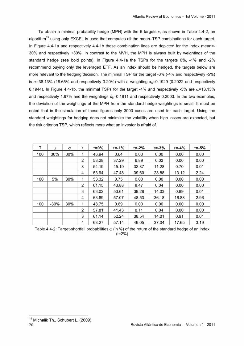
To obtain a minimal probability hedge (MPH) with the 6 targets τ, as shown in Table 4.4-2, an

algorithm15 using only EXCEL is used that computes all the mean–TSP combinations for each target.

In Figure 4.4-1a and respectively 4.4-1b these combination lines are depicted for the index mean=-

30% and respectively +30%. In contrast to the MVH, the MPH is always built by weightings of the

standard hedge (see bold points). In Figure 4.4-1a the TSPs for the targets 0%, -1% and -2%

recommend buying only the leveraged ETF. As an index should be hedged, the targets below are

more relevant to the hedging decision. The minimal TSP for the target -3% (-4% and respectively -5%)

is α=38.13% (18.65% and respectively 3.20%) with a weighting xS=0.1929 (0.2022 and respectively

0.1944). In Figure 4.4-1b, the minimal TSPs for the target -4% and respectively -5% are α=13.13%

and respectively 1.97% and the weightings xS=0.1911 and respectively 0.2003. In the two examples,

the deviation of the weightings of the MPH from the standard hedge weightings is small. It must be

noted that in the simulation of these figures only 3000 cases are used for each target. Using the

standard weightings for hedging does not minimize the volatility when high losses are expected, but

the risk criterion TSP, which reflects more what an investor is afraid of.

T µ σ λ τ=0% τ=-1% τ=-2% τ=-3% τ=-4% τ=-5%

100 30% 30% 1 46.94 0.64 0.00 0.00 0.00 0.00 2 53.28 37.29 6.89 0.03 0.00 0.00 3 54.19 45.19 32.37 11.28 0.70 0.01 4 53.94 47.48 39.60 28.88 13.12 2.24

100 5% 30% 1 53.32 0.75 0.00 0.00 0.00 0.00 2 61.15 43.88 8.47 0.04 0.00 0.00 3 63.02 53.61 39.28 14.03 0.89 0.01 4 63.69 57.07 48.53 36.18 16.88 2.96

100 -30% 30% 1 48.75 0.69 0.00 0.00 0.00 0.00 2 57.81 41.43 8.11 0.04 0.00 0.00 3 61.14 52.24 38.54 14.01 0.91 0.01 4 63.27 57.14 49.05 37.04 17.65 3.19

Table 4.4-2: Target-shortfall probabilities α (in %) of the return of the standard hedge of an index (i=2%)

15 Michalik Th., Schubert L. (2009).



21

Figure 4.4-1a: Mean–TSP mix of an index (T=100, µ=-30%, σ=30%) and short ETF (λ=4)

µ=µP ρ λ τ=0% τ=-2% τ=-4% τ=-10% τ=-15% τ=-20% 30% 0.75 1 45.20 32.05 20.58 2.61 0.16 0.00

2 45.67 35.75 26.46 7.17 1.36 0.13 3 45.65 36.93 28.62 9.69 2.50 0.38 4 45.61 37.57 29.82 11.33 3.41 0.65

5% 0.75 1 47.43 33.89 21.94 2.84 0.18 0.00 2 49.27 39.10 29.39 8.37 1.66 0.17 3 50.56 41.61 32.85 11.85 3.25 0.53 4 51.71 43.46 35.23 14.36 4.62 0.95

-30% 0.75 1 45.86 32.58 20.95 2.67 0.17 0.00 2 48.00 38.28 28.98 8.53 1.75 0.19 3 49.92 41.56 33.25 12.65 3.67 0.64 4 51.86 44.27 36.54 15.94 5.51 1.23

Table 4.4-3: TSPs α (in %) of the return of the standard hedge of a portfolio (T: 100, σ=30%, i=2%)



22

Figure 4.4-1b: Mean–TSP mix of an index (T=100, µ=+30%, σ=30%) and short ETF (λ=4)

In most cases, the underlying index of the inverse ETF is not identical to the assets that have to

be hedged. Therefore, the correlation ρ between the return of the underlying index and the assets or

portfolio again has to be taken into consideration. Table 4.4-3 depicts the TSP for different means µ,

leverage factors λ and correlation ρ=0.75. In general, the probability of falling short of a very negative

target becomes greater than in the case of ρ=1.00 (this ρ can be supposed to be the values of Table

4.4-2). However, the TSP for the target τ=0 is always smaller than that in Table 4.4-2. It must be

pointed out that the two tables do not have the same targets in the columns.

Figure 4.4-2a: Mean–TSP mix of a portfolio (ρ: 0.75; index: T=100, µ=-30%, σ=30%) and leveraged

short ETF (λ=4)



23

To gain some insights into the TSP when portfolios have to be hedged by inverse ETFs, the

mean–TSP space is used. In the examples again the leverage factor λ=4 is applied to show the

difference between the standard hedge (with xS=0.20) and the MPH. In Figure 4.4-2a the mean–TSP

lines are plotted, when the mean µ=µP=-30%. Such negative expectations may be the reason to start

hedging at the beginning of a bearish market. The minimal TSP mix in the chart is more or less where

the mean–TSP mix of the standard hedge can be found (bold points). Similar results can be observed

for other leverage factors, but for small or high positive returns, this characteristic of the standard

hedge can not be found. Figure 4.4-2b shows for a mean µ=µP=+30% that the minimal mean–TSP

point is not where the standard hedge is located. Especially the mean–TSP lines for τ=-10% to -20%

show that the reduction of the TSP would be possible. This could be achieved if a smaller part of the

budget (xS=0.11 to 0.13) is invested in the inverse ETF. For the target τ=-10% the TSPHedge=11.33.

However, the TSP of the MPH is only TSPMPH=8.57. This feature of the standard hedge seems not to

be very important due to the reason that positive expectations will in most cases not initiate hedging

transactions. Table 4.4-4 contains for these 2 figures the minimal TSP and the weighting xS.

Figure 4.4-2b: Mean–TSP mix of a portfolio (ρ: 0.75; index: T=100, µ=+30%, σ=30%) and leveraged

short ETF (λ=4)



24

µ=µP=-30% µ=µP=+30%

Target τ=-10% τ=-15% τ=-20% τ=-10% τ=-15% τ=-20% xPortfolio 0.79 0.80 0.80 0.89 0.87 0.87

xS 0.21 0.20 0.20 0.11 0.13 0.13 TSPMPH 15.83 5.60 1.43 8.57 2.67 0.53 xPortfolio 0.80 0.80 0.80 0.80 0.80 0.80

xS 0.20 0.20 0.20 0.20 0.20 0.20 TSPHedge 15.94 5.51 1.23 11.33 3.41 0.65

Table 4.4-4: TSP of the MPH and standard hedge (ρ=0.75, T=100, lev.: 4, σ=30%, i=2%)16 5. Conclusion and preview

The standard hedge that uses weightings only determined by the leverage factor seems to be a

good recommendation, even in cases when strong losses are expected. The hedge of the value of an

index and a short or leveraged ETF causes positive skewness than cannot be ignored. Therefore,

minimizing the variance of the hedge return leads to confusing results: when the underlying index has

high losses, the minimal variance hedge (MVH) will elevate the part of this index in the hedge mix (due

to the lower volatility) and not the part of the short or leveraged ETF as is usually expected.

Furthermore, the standard hedge and the MVH mix their hedges in different ways. In contrast, the risk

measure target-shortfall probability (TSP) seems to select in a similar way to the standard hedge. In

the case when strong increasing or decreasing index prices are supposed, different leverage factors

seem to lead to the same weightings as the standard hedge. This feature of minimizing the TSP can

be observed even when a portfolio (which has a higher correlation e.g. ρ=0.75 with the return of the

index) has to be hedged by an inverse ETF. The mean return of the underlying index of this ETF is

supposed to have a negative development. Due to the skewness the risk measure TSP seems to be

more appropriate to reduce the risk investors are afraid of: it is the probability of losing. The volatility is

less appropriate for this type of hedging. Therefore, hedging should not be evaluated by this risk

measure.

More dynamic hedge approaches – like rebalancing the weightings to those of the standard

hedge17 – have to be evaluated in the same way. Although this hedge approach was not investigated

in this paper, some remarks may be added in this place. If the price of an index increases (and

respectively decreases) very strongly, the hedge would produce profits that will be avoided by

rebalancing. Certainly in these cases the profits will be reduced, but whether the losses will be too

depends on the upper and lower price limits, where rebalancing will be performed. If these limits have

too great a distance, low transaction costs have to be paid but the losses will remain. Losses occur

16 Due to the small number of 3000 points in the scatter plot example, the TSPMPH in not always smaller than the TSPHedge. 17 See Hill, J., Teller, S. (2010).



25

when the index price goes to the side.18 If the limits are close together, the rebalancing will cause

higher transaction costs but then the losses can be reduced. The benefit of this dynamic hedging

approach needs to be invested in detail.

Another proposal to reduce the losses of a hedge is the integration of a further instrument that is

able to compensate for the losses of the hedge discussed in this paper. This instrument could be a

short straddle or short strangle, having the index as the underlying feature. As these derivatives

generate profit when the index goes aside, part of the losses can be reduced. On the other side, if

strong increasing or decreasing index prices occur, the short straddle and the short strangle would

have a negative return. Whether this hedging duo (e.g. short ETF and strangle) works well depends

among other things on the offered exercise prices in the option market and respectively in the

exchange boards. To gain more insights, further research is necessary.

18 See Michalik Th., Schubert L. (2009).



26

6. References [1] Alexander, C., Barbosa, A. (2007): Hedging and Cross Hedging ETFs, International Capital

Markets Association (ICMA), Discussion Paper in Finance DP2007-01, January 2007.

[2] Bamberg, G., Baur, F. (1996): Statistik, Oldenbourg.

[3] Deutsch, H. P. (2004): Derivate und Interne Modelle – Modernes Risikomanagement, Stuttgart,

pp. 26–34.

[4] Flood, Ch. (2010): Risk betting on short and leveraged ETFs, Financial Times (online version),

2nd November 2010.

[5] Grundmann, W., Luderer B. (2003): Formelsammlung Finanzmathematik,

Versicherungsmathematik, Wertpapieranalyse, Teubner.

[6] Hill, J., Teller, S. (2010): Hedging With Inverse ETFs, Journal of Indexes, November/December

2010, pp. 18–24.

[7] Luenberger, D. G. (1998): Investment Science, Oxford University Press, New York, p. 309.

[8] Michalik, T., Schubert, L. (2009): Hedging with Short ETFs, Economics Analysis Working

Papers, Vol. 8 No. 9, ISSN 15791475.

[9] Szeby, S. (2002): Die Rolle der Simulation im Finanzmanagement, Stochastik in der Schule 22,

Vol. 3, pp. 12–22.



27

Appendix: A1: Proof of the immunization of the index value by short ETFs A2: Proof of formula (2-6): generation of a variable YP that has a correlation ρ with Y A3: Simulated examples for a minimal variance hedge of an index with different means µ A4: Simulated examples for a minimal variance hedge of a portfolio with different correlations



28

A1: Proof of the immunization of the index value by short ETFs In the case of T=1, for leverage factor λ the weightings xI=λ/(λ+1) for the index and xS=1/(λ+1)

for the short ETF (with xI+xS=1) immunized the index against changing prices.

Proof:

The value of the hedge H1 in t=1 depends on the distribution of the budget B to the index (I0) and to

the short ETF (S0) in t=0. These weightings are denominated by xI and xS with xI+xS=1. The budget B

invested in the index is I0=B·xI and S0=B·xS. In t=0 the investment would be H0=I0+S0=B·xI+B·xS=B. In

t=1 the hedge value is

S1I11 xSxIH ⋅+⋅= . (A1-1)

The return of I0 within one day is r1 and respectively the development factor I1/I0=1+r1. The value of the

index after one day is I1=I0·(1+r1). The value S1 is the short ETF and can be determined by equation

(2-3):

⎟⎠⎞

⎜⎝⎛⋅⋅+λ+⎟⎟

⎠

⎞⎜⎜⎝

⎛⋅λ−+λ⋅=

360iS)1(

II)1(SS 00

101 .

In I1 and S1, the values I0 and S0 can be replaced by I0=B·xI and S0=B·xS. By this hedge equation (A1-

1) can be transformed to

( )( ) ⎟⎟⎠

⎞⎜⎜⎝

⎛⎟⎠⎞

⎜⎝⎛⋅⋅⋅+λ++⋅λ−+λ⋅⋅++⋅⋅=

360ixB)1(r1)1(xB)r1(xBH S1S1I1 (A1-2)

and with xI=λ/(λ+1) and respectively xS=1/(λ+1) to

( ) ⎟⎠⎞

⎜⎝⎛

+λ⋅⎟⎟⎠

⎞⎜⎜⎝

⎛⎟⎠⎞

⎜⎝⎛⋅+⎟

⎠⎞

⎜⎝⎛⋅λ⋅+⋅λ⋅−λ⋅−+λ⋅+⎟

⎠⎞

⎜⎝⎛

+λλ

⋅⋅+=1

1360

iB360

iBrBBBB1

rBBH 111 . (A1-3)

In equation (A1-3) the part B·λ-B·λ is zero. Now the equation (A1-3) becomes

⎟⎠⎞

⎜⎝⎛⋅

+λ+⎟

⎠⎞

⎜⎝⎛⋅λ⋅

+λ+⋅

+λλ⋅

−+λ

+⋅+λλ⋅

++λλ⋅

=360

i1

B360

i1

Br1

B1

Br1

B1

BH 111 or (A1-4)

⎟⎠⎞

⎜⎝⎛⋅

+λ+⎟

⎠⎞

⎜⎝⎛⋅λ⋅

+λ+

+λ+

+λλ⋅

=360

i1

B360

i1

B1

B1

BH1 . (A1-5)



29

Some transformations show that for T=1 only the interest rate i/360 can be earned by the perfect

hedge:

⎟⎠⎞

⎜⎝⎛ +⋅=⎟⎟

⎠

⎞⎜⎜⎝

⎛⎟⎠⎞

⎜⎝⎛⋅+λ++λ⋅

+λ=

360i1B

360i)1(1

1BH1 ■ (A1-6)

A2: Proof of formula (2-6): generation of a variable YP that has a correlation ρ with Y (variables Y ( YP ) offer the random numbers for the index return (portfolio return)).

For the generation of a stochastic variable YP that has a correlation of ρ with another variable

Y, a third variable Y’ is used. The variables Y and Y’ have the same mean µ and variance σ2.

Using normal distributed random numbers y, y’, a realization of the variable yP can be computed19 by

'yρ1yρy 2P ⋅−+⋅= (A2-1)

Proof:

1.) The variable YP will have variance σ2 like Y and Y’:

σP2 = ρ2 σ2 + (1 - ρ2) σ2 = σ2. (A2-2)

The expected value µP of YP is:

µ⋅⎟⎠⎞⎜

⎝⎛ ρ−+ρ=µ⋅ρ−+µ⋅ρ=µ 22

P 11 .20 (A2-3)

2.) The parameter ρ is the correlation corr(y,yP):

Equation (A2-1) can be transformed to

y1

y1

1'y2P2⋅

ρ−

ρ−⋅

ρ−= . (A2-4)

The variance σ2 of Y’ is

19 The formula (A2-1) was mentioned by Siegfried Szeby (2002) without source or proof. 20 The expected value µP is not necessary for the following proof. As Y and Y’ are N(0,1) distributed, the expected value µP=0 and respectively YP~N(0,1).



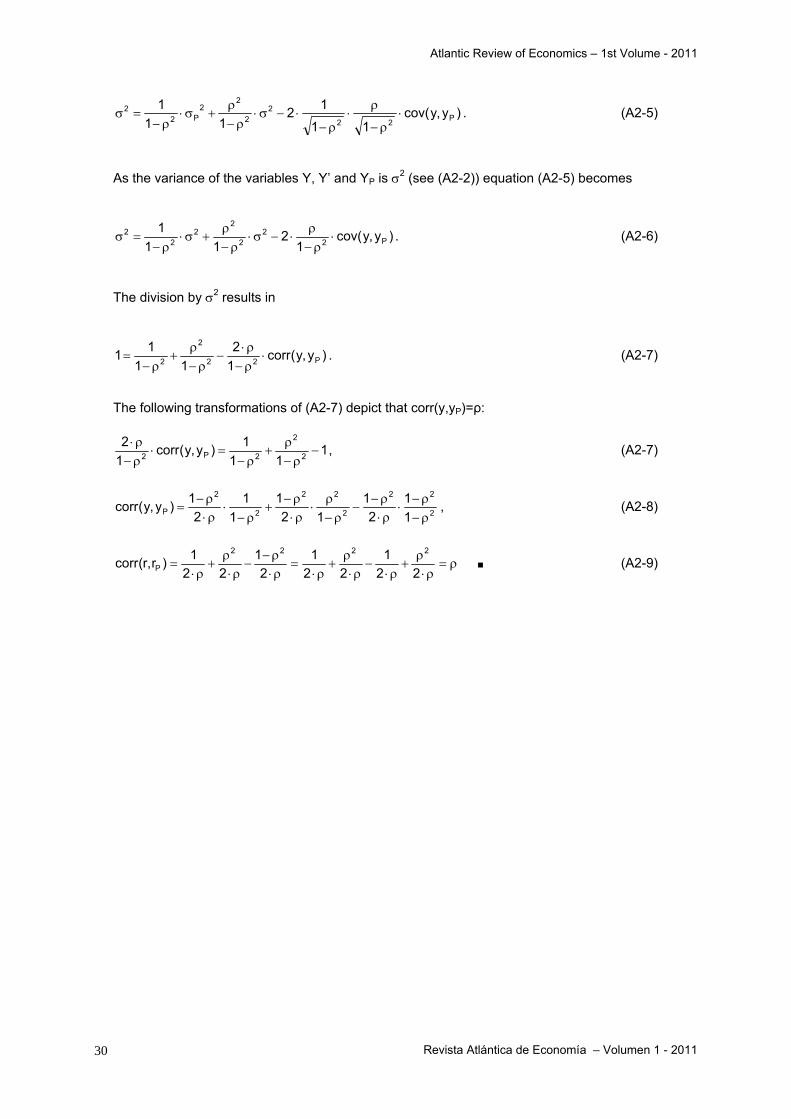
30

)y,ycov(11

1211

1P22

22

22

P22 ⋅

ρ−

ρ⋅

ρ−⋅−σ⋅

ρ−ρ

+σ⋅ρ−

=σ . (A2-5)

As the variance of the variables Y, Y’ and YP is σ2 (see (A2-2)) equation (A2-5) becomes

)y,ycov(1

211

1P2

22

22

22 ⋅

ρ−ρ

⋅−σ⋅ρ−

ρ+σ⋅

ρ−=σ . (A2-6)

The division by σ2 results in

)y,y(corr12

1111 P22

2

2 ⋅ρ−ρ⋅

−ρ−

ρ+

ρ−= . (A2-7)

The following transformations of (A2-7) depict that corr(y,yP)=ρ:

111

1)y,y(corr12

2

2

2P2 −ρ−

ρ+

ρ−=⋅

ρ−ρ⋅ , (A2-7)

2

22

2

22

2

2

P 11

21

121

11

21)y,y(corr

ρ−ρ−

⋅ρ⋅ρ−

−ρ−

ρ⋅

ρ⋅ρ−

+ρ−

⋅ρ⋅ρ−

= , (A2-8)

ρ=ρ⋅

ρ+

ρ⋅−

ρ⋅ρ

+ρ⋅

=ρ⋅ρ−

−ρ⋅

ρ+

ρ⋅=

221

221

21

221)r,r(corr

2222

P ■ (A2-9)



31

A3: Simulated examples for a minimal variance hedge of an index with different

means µ

λ µ

1 2 3 4

30% xI =0.454888 xS=0.545112 corr: -0.975498 rI: 0.100615 rS : -0.081332 sI

2: 0.030671 sS

2: 0.021453

xI =0.612047 xS=0.387953 corr: -0.945504 rI : 0.100582 rS : -0.160764 sI

2: 0.030660 sS

2: 0.074467

xI =0.696247 xS=0.303753 corr: -0.904617 rI: 0.100556 rS : -0.233360 sI

2 : 0.030650 sS

2: 0.149335

xI =0.752358 xS=0.247642 corr: -0.852972 rI: 0.100646 rS : -0.299933 sI

2 : 0.030675 sS

2: 0.243411 20% xI =0.468730

xS=0.531270 corr: -0.975524 rI: 0.070420 rS: -0.055400 sI

2: 0.028989 sS

2: 0.022635

xI =0.631947 xS=0.368053 corr: -0.945586 rI: 0.070473 rS: -0.112744 sI

2: 0.029019 sS

2: 0.083123

xI =0.720033 xS=0.279967 corr: -0.904587 rI: 0.070405 rS: -0.166436 sI

2: 0.029013 sS

2: 0.176312

xI =0.778494 xS=0.221506 corr: -0.853781 rI: 0.070364 rS: -0.217004 sI

2 : 0.028992 sS

2: 0.303164 10% xI =0.482546

xS=0.517454 corr: -0.975536 rI: 0.041133 rS: -0.028785 sI

2: 0.027448 sS

2: 0.023910

xI =0.651427 xS=0.348573 corr: -0.945721 rI: 0.041032 rS: -0.061817 sI

2: 0.027431 sS

2: 0.092699

xI =0.742503 xS=0.257497 corr: -0.904749 rI: 0.041072 rS: -0.093890 sI

2: 0.027430 sS

2: 0.207736

xI =0.802352 xS=0.197648 corr: -0.853962 rI: 0.041068 rS: -0.124863 sI

2: 0.027438 sS

2: 0.377164 5% xI =0.489570

xS=0.510430 corr: -0.975527 rI: 0.026746 rS: -0.015179 sI

2: 0.026679 sS

2: 0.024568

xI =0.661004 xS=0.338996 corr: -0.945601 rI: 0.026779 rS: -0.035517 sI

2: 0.026697 sS

2: 0.098000

xI =0.753210 xS=0.246790 corr: -0.904846 rI: 0.026696 rS: -0.055207 sI

2: 0.026693 sS

2: 0.225536

xI =0.813651 xS=0.186349 corr: -0.853823 rI : 0.026768 rS: -0.074756 sI

2: 0.026716 sS

2: 0.421736 0% xI =0.496573

xS=0.503427 corr: -0.975566 rI: 0.012518 rS: -0.001333 sI

2: 0.025947 sS

2: 0.025253

xI =0.670361 xS=0.329639 corr: -0.945625 rI: 0.012619 rS: -0.008355 sI

2: 0.025968 sS

2: 0.103476

xI =0.763601 xS=0.236399 corr: -0.904997 rI: 0.012559 rS: -0.015111 sI

2: 0.025953 sS

2: 0.244657

xI =0.824362 xS=0.175638 corr: -0.854101 rI: 0.012573 rS: -0.021915 sI

2: 0.025952 sS

2: 0.470333 -5% xI =0.503456

xS=0.496544 corr: -0.975539 rI: -0.001329 rS: 0.012525 sI

2: 0.025255 sS

2: 0.025955

xI =0.679681 xS=0.320319 corr: -0.945722 rI: -0.001411 rS: 0.019659 sI

2: 0.025234 sS

2: 0.109252

xI =0.773790 xS=0.226210 corr: -0.904928 rI: -0.001348 rS: 0.026698 sI

2: 0.025253 sS

2: 0.265870

xI =0.834341 xS=0.165659 corr: -0.854289 rI: -0.001371 rS: 0.033726 sI

2: 0.025245 sS

2: 0.523604 -10% xI =0.510437

xS=0.489563 corr: -0.975562 rI: -0.015122 rS : 0.026689 sI

2: 0.024548 sS

2: 0.026659

xI =0.688701 xS=0.311299 corr: -0.945754 rI: -0.015114 rS: 0.048249 sI

2: 0.024560 sS

2: 0.115369

xI =0.783409 xS=0.216591 corr: -0.905273 rI: -0.015190 rS: 0.070405 sI

2: 0.024545 sS

2: 0.287943

xI =0.844223 xS=0.155777 corr: -0.854200 rI: -0.015200 rS: 0.093138 sI

2: 0.024551 sS

2: 0.585772 -20% xI =0.524364

xS=0.475636 corr: -0.975571 rI: -0.042166 rS: 0.055644 sI

2: 0.023209 sS

2: 0.028141

xI =0.706563 xS=0.293437 corr: -0.945825 rI: -0.042163 rS: 0.108214 sI

2: 0.023224 sS

2: 0.128733

xI =0.802063 xS=0.197937 corr: -0.905333 rI: -0.042173 rS: 0.163265 sI

2: 0.023210 sS

2: 0.339243

xI =0.861931 xS=0.138069 corr: -0.854764 rI: -0.042136 rS: 0.221097 sI

2: 0.023228 sS

2: 0.727582 -30% xI =0.538233

xS=0.461767 corr: -0.975611 rI: -0.068443 rS: 0.085402 sI

2: 0.021967 sS

2: 0.029734

xI =0.723670 xS=0.276330 corr: -0.945869 rI: -0.068367 rS: 0.171364 sI

2: 0.021987 sS

2: 0.143627

xI =0.819466 xS=0.180534 corr: -0.905352 rI: -0.068439 rS: 0.264305 sI

2: 0.021967 sS

2: 0.400104

xI =0.877992 xS=0.122008 corr: -0.855066 rI: -0.068447 rS: 0.364380 sI

2: 0.021961 sS

2: 0.904905

Table A3: MVH: index & short ETF (T=100, σ=30%, i=2%)



32

A4: Simulated examples for a minimal variance hedge of a portfolio with different correlations

For the examples in appendix A4, a portfolio should be hedged by a short index ETF. The returns of

the index and of the portfolio have a correlation ρ. For the following Table A4 the mean return of the

index is supposed to be µP=µ=5%.

ρ

T 0.95 0.90 0.85 0.80 0.75

1 xP=0.499977 xS=0.500023 corr: -0.949970 rP: 0.000264 rS: -0.000155 sP

2: 0.000250 sS

2: 0.000250

xP=0.499997 xS=0.500003 corr: -0.900055 rP: 0.000254 rS: -0.000150 sP

2: 0.000250 sS

2: 0.000250

xP=0.500045 xS=0.499955 corr: -0.850011 rP: 0.000273 rS: -0.000154 sP

2: 0.000250 sS

2: 0.000250

xP=0.499988 xS=0.500012 corr: -0.799873 rP: 0.000267 rS: -0.000156 sP

2: 0.000250 sS

2: 0.000250

xP=0.500085 xS=0.499915 corr: -0.750050 rP: 0.000272 rS: -0.000157 sP

2: 0.000250 sS

2: 0.000250 5 xP=0.499573

xS=0.500427 corr: -0.949053 rP: 0.001328 rS: -0.000772 sP

2: 0.001254 sS

2: 0.001250

xP=0.499549 xS=0.500451 corr: -0.899077 rP: 0.001308 rS: -0.000755 sP

2: 0.001254 sS

2: 0.001250

xP=0.499475 xS=0.500525 corr: -0.849360 rP: 0.001332 rS: -0.000766 sP

2: 0.001255 sS

2: 0.001250

xP=0.499619 xS=0.500381 corr: -0.799378 rP: 0.001339 rS: -0.000771 sP

2: 0.001255 sS

2: 0.001251

xP=0.499564 xS=0.500436 corr: -0.749495 rP: 0.001321 rS: -0.000758 sP

2: 0.001254 sS

2: 0.001250 10 xP=0.499048

xS=0.500952 corr: -0.947869 rP: 0.002643 rS: -0.001521 sP

2: 0.002516 sS

2: 0.002497

xP=0.498994 xS=0.501006 corr: -0.898047 rP: 0.002635 rS: -0.001510 sP

2: 0.002516 sS

2: 0.002496

xP=0.499025 xS=0.500975 corr: -0.848212 rP: 0.002655 rS: -0.001545 sP

2: 0.002516 sS

2: 0.002498

xP=0.498930 xS=0.501070 corr: -0.798426 rP: 0.002662 rS: -0.001552 sP

2: 0.002515 sS

2: 0.002496

xP=0.498985 xS=0.501015 corr: -0.748629 rP: 0.002630 rS: -0.001500 sP

2: 0.002517 sS

2: 0.002499 50 xP=0.494741

xS=0.505259 corr: -0.938687 rP: 0.013250 rS: -0.007602 sP

2: 0.012903 sS

2: 0.012388

xP=0.494503 xS=0.505497 corr: -0.889540 rP: 0.013317 rS: -0.007658 sP

2: 0.012921 sS

2: 0.012395

xP=0.494451 xS=0.505549 corr: -0.840375 rP: 0.013327 rS: -0.007667 sP

2: 0.012909 sS

2: 0.012392

xP=0.494216 xS=0.505784 corr: -0.791169 rP: 0.013312 rS: -0.007611 sP

2: 0.012918 sS

2: 0.012394

xP=0.494208 xS=0.505792 corr: -0.741927 rP: 0.013279 rS: -0.007607 sP

2: 0.012911 sS

2: 0.012400 100 xP=0.489308

xS=0.510692 corr: -0.927308 rP: 0.026690 rS: -0.015115 sP

2: 0.026670 sS

2: 0.024560

xP=0.489022 xS=0.510978 corr: -0.879130 rP: 0.026776 rS: -0.015218 sP

2: 0.026703 sS

2: 0.024588

xP=0.488623 xS=0.511377 corr: -0.830804 rP: 0.026769 rS: -0.015189 sP

2: 0.026705 sS

2: 0.024570

xP=0.488491 xS=0.511509 corr: -0.782415 rP: 0.026699 rS: -0.015155 sP

2: 0.026679 sS

2: 0.024577

xP=0.488038 xS=0.511962 corr: -0.733946 rP: 0.026755 rS: -0.015175 sP

2: 0.026693 sS

2: 0.024567 300 xP=0.466934

xS=0.533066 corr: -0.883189 rP: 0.082368 rS: -0.044818 sP

2: 0.091251 sS

2: 0.071105

xP=0.466112 xS=0.533888 corr: -0.838286 rP: 0.082320 rS: -0.044785 sP

2: 0.091218 sS

2: 0.071070

xP=0.465182 xS=0.534818 corr: -0.793203 rP: 0.082428 rS: -0.044845 sP

2: 0.091259 sS

2: 0.071060

xP=0.464536 xS=0.535464 corr: -0.748087 rP: 0.082397 rS: -0.044863 sP

2: 0.091251 sS

2: 0.071178

xP=0.463433 xS=0.536567 corr: -0.702106 rP: 0.082330 rS: -0.044690 sP

2: 0.091213 sS

2: 0.071075

Table A4-1: MVH: portfolio & short index ETF (µP=µ=5%, σ=30%, i=2%, leverage factor: 1)



33

ρ T

0.95 0.90 0.85 0.80 0.75

100 xP=0.818042 xS=0.181958 corr: -0.813167 rP: 0.026695 rS: -0.074771 sP

2: 0.026671 sS

2: 0.421193

xP=0.822466 xS=0.177534 corr: -0.772389 rP: 0.026741 rS: -0.074904 sP

2: 0.026687 sS

2: 0.421062

xP=0.827010 xS=0.172990 corr: -0.731472 rP: 0.026723 rS: -0.074830 sP

2: 0.026687 sS

2: 0.420565

xP=0.831961 xS=0.168039 corr: -0.689847 rP: 0.026717 rS: -0.074839 sP

2: 0.026673 sS

2: 0.420828

xP=0.836880 xS=0.163120 corr: -0.648594 rP: 0.026771 rS: -0.075030 sP

2: 0.026684 sS

2: 0.420772

Table A4-2: MVH: portfolio & short index ETF (µP=µ=5%, σ=30%, i=2%, leverage factor: 4)

Hedge ratios for short and leveraged ETFs Review of Economics – 1st Volume - 2011 Revista...

Documents

Transcript of Hedge ratios for short and leveraged ETFs Review of Economics – 1st Volume - 2011 Revista...