Constructing Strategic Hedge Fund Portfolios

Peter CarlBrian Peterson

● Discuss the challenges of constructing hedge fund portfolios

● Offer a framework for considering strategic allocation using hedge fund indexes

● Show the relative performance of multiple objectives

● Discuss extensions to the framework

Introduction

Introduction

● The code presented in these slides is necessarily incomplete.

● For the actual code needed to replicate these slides, see:

● Functions are very compute intensive

● Standard disclaimers apply: no warranty, guarantees, etc.

https://r-forge.r-project.org/scm/viewvc.php/pkg/PortfolioAnalytics/sandbox/script.workshop2010.R?root=returnanalytics&view=log

Objectives

● Random Portfolios can help you build intuition about your objectives and constraints

● Rebalancing periodically and examining out

of sample performance will help refine objectives

● Analytic solvers and parallel computation are

valuable as things get more complex

Not only true in the context of strategic allocation

Strategic allocation

...broadly described as periodically reallocating the portfolio to achieve a long-term goal● Understand the nature and sources of investment risk

within the portfolio● Manage the resulting balance of risk and return of the

portfolio● Applied within the context of the current economic and

market situation● Think systematically about preferences and constraints

● Strategic allocations can be part of a larger layered optimization set, where you do

○ strategic rebalancing with strategic objectives on a longer timeframe

○ periodic rebalancing on capital inflows and outflows○ rebalancing inside a sub-portfolio or style portfolio to

optimize the performance of that sub-portfolio■ possibly with different objectives and constraints

for each sub-portfolio○ tactical rebalancing to take advantage of short-lived

opportunities○ and capital allocation among strategies or even stratgy

configurations in a higher-frequency world● All these layers can and should co-exist, in a top-down or

bottom-up view of the whole portfolio

Low Frequency Allocation

A portfolio of hedge funds presents:

● Very high transaction costs

● Liquidity constraints

● Long investment horizons

● Slow rebalancing cycles

● Monthly data

● Little feedback about decisions

Take a complicated situation and make it worse.

● Provides numerical solutions to portfolios with complex constraints and objectives

● Unifies the interface into different numerical optimizers

● Implements a front end to two analytical solvers: Differential Evolution and Random Portfolios

● Preserves the flexibility to define any kind of objective and constraint

● Work-in-progress, available on R-Forge in the ReturnAnalytics project

PortfolioAnalytics

GSoC 212 project to add additional closed form and global optimizers to the package: http://rwiki.sciviews.org/doku.php?id=developers:projects:gsoc2012:portfolioanalytics

Other Packages

PerformanceAnalytics● Library of econometric functions for performance and

risk analysis of financial portfolios

rugarch and rmgarch● By Alexios Ghalanos● The univariate and multivariate GARCH parts of the

rgarch project on R-Forge

xts● By Jeff Ryan and Josh Ulrich● Time series package specifically for finance

RGarch: comprehensive set of methods for modelling GARCH processes, including fitting, filtering, forecasting, simulation as well as diagnostic tools including plots and various tests xts offers relatively lossless conversion to and from the myriad of time-series classes in R

Selected Hedge Fund Styles

Relative Value ● Fixed Income Arb

● Convertible Arb

● Equity Market Neutral

● Event Driven

Directional● Equity Long/Short

● Macro

● CTA

Monthly data from the EDHEC hedge fund peer group indexes

● meta-index that combines competing hedge fund indexes● captures a very large fraction of the information contained in the competing

indexes● selected to be representative, not necessarily investible

discuss style definitions

Performance of EDHEC Indexes

Varying degrees of smoothness and choppinessPast episodes of both high dispersion and high correlationSmall drawdowns tend to be dispersed among styles through timelarger, coincident drawdowns in 1998 and 2008

Performance of EDHEC Indexes

easier to see relative volatilitycoincident drawdownsequity and credit affected in 1998, CTA's were not; again in 2008Risk estimates fairly stable through time; portfolio effects of looking at indexes

Rolling 36-Month Performance

Relative long-term stability of returns, volatility regimes and window effectsdownward drift through last decade reversing?

Performance of Indexes

From January 1997 to February 2012

Easier to see which index has been outperforming its long term average here

Performance of Indexes

Distributions

From January 1997 to February 2012

95% CI shows downside outliers for all the RV strategies and ELS, upside outliers for GM

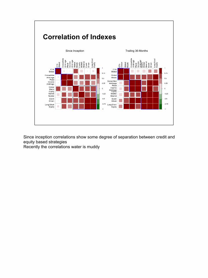
Correlation of Indexes

Since Inception Trailing 36-Months

Since inception correlations show some degree of separation between credit and equity based strategiesRecently the correlations water is muddy

Portfolio Issues

Markowitz (1952) described an investor's objectives as:● maximizing some measure of gain while● minimizing some measure of risk.

Many approaches follow Markowitz and use mean return and standard deviation of returns for “risk”.

Describes the academic approach. Real investors often have more complex objectives. Std Dev was a simplification, even for Markowitz who recommended downside deviation in the text of his Nobel speech

Portfolio Issues

Most investors would prefer:

● to be approximately correct rather than precisely wrong

● to define risk as potential loss rather than volatility

● the flexibility to define any kind of objective and combine constraints

● a framework for considering different sets of portfolio constraints for comparison through time

● to build intuition about optimization through visualization

Portfolio Issues

Construct a portfolio that:● maximizes return,● with per-asset conditional constraints,● with a specific univariate risk limit,● while minimizing component risk concentration,● and limiting drawdowns to a threshold value.

Not a quadratic (or linear, or conical) problem any more.

Risk rather than volatility

● Expected Tail Loss (ETL) is also called Conditional Value-at-Risk (CVaR) and Expected Shortfall (ES)

● ETL is the mean expected loss when the loss exceeds the VaR

● ETL has all the properties a risk measure should have to be coherent and is a convex function of the portfolio weights

● Returns are skewed and/or kurtotic, so we use Cornish-Fisher (or “modified”) estimates of ETL instead

Use Random Portfolios

Burns (2009) describes Random Portfolios● From a portfolio seed, generate random permutations

of weights that meet your constraints on each asset.● More from Pat at http://www.portfolioprobe.com/blog/

Sampling can help provide insight into the goals and constraints of the optimization● Covers the 'edge case'(min/max) constraints well● Covers the 'interior' portfolios● Useful for finding the search space for an optimizer● Allows arbitrary number of samples● Allows massively parallel execution

Add General Constraints

Constraints specified for each asset in the portfolio:● Maximum position: 30%● Minimum position: 5%● Weights sum to 100%● Weight step size of 0.5%

Other settings:● Confidence for VaR/ETL set p=1-1/12● Random portfolios with 4000 permutations● Rebalancing quarterly

Add General Constraints# Select a rebalance period using endpoints identifiers from xtsrebalance_period = 'quarters'clean = "boudt" # slow! may use: "none"permutations = 4000p = 1-(1/12) # Obs one month per year # A set of box constraints used to initialize ALL the objective portfoliosinit.constr <- constraint(assets = colnames(edhec.R), min = .05, # minimum position weight max = .3, # maximum position weight min_sum=0.99, # minimum sum of weights must be near 1 max_sum=1.01, # maximum sum must also be about 1 weight_seq = generatesequence(by=0.005) )

Add Measures# Add measure 1, annualized returninit.constr <- add.objective(constraints=init.constr, type = "return", # the kind of objective this is name = "pamean", enabled = TRUE, # enable or disable the objective multiplier = 0, # calculate it but don't use it in the objective arguments = list(n=60) # for five years of monthly data)

Add Measures# Add measure 2, annualized standard deviationinit.constr <- add.objective(init.constr, type = "risk", # the kind of objective this is name = "pasd", # to minimize from the sample #name='pasd.garch', # to minimize from the predicted sigmas enabled = TRUE, # enable or disable the objective multiplier = 0, # calculate it but don't use it in the objective arguments = list() # from inception for pasd #arguments=list(sigmas=garch.sigmas) # from inception for pasd.garch)

Add Measures# Add measure 3, CVaR with p=(1-1/12)init.constr <- add.objective(init.constr, type = "risk", # the kind of objective this is name = "CVaR", # the function to minimize enabled = FALSE, # enable or disable the objective multiplier = 0, # calculate it but don't use it in the objective arguments=list(p=p), clean = clean)

Improving our Estimates

● The optimizer chooses portfolios based on forward looking estimates of risk and return based on the portfolio moments

● Estimates use the first four moments and co-moments ○ return, volatility/covariance, (co)skewness, (co)kurtosis

● The historical sample moments work fine as predictors in normal market regimes, but very poorly when the market regime shifts

One of the largest challenges in portfolio optimization is improving the estimates of return and volatility

Can we improve on the historical sample moments? Estimation error is one of the largest problems in optimization. If you're going to do optimization, you should work on improving your estimates.

Returns ● ARMA(1,1) to try to capture

some of the time varying return structure

● Preserves the observed autocorrelation of the series

● Approaches the long-run means of the series near the end, losing time-varying structure

● Merely illustrative of what is possible with a more sophisticated model

● Model specification close to defaults in rugarch

● Standard GARCH(1,1) framework

● Uses Dynamic Conditional Correlation to capture interdependencies among the series

● Modeled an asymmetric generalized hyperbolic distribution to allow for coskewness and cokurtosis of the return series

● Used rmgarch, little tuning of the specification for this example

VolatilityForecasting

Illustrative only, we didn't really examine and won't discuss model fit here Even with a merely illustrative example, the out of sample estimation error is markedly reduced. This should lend more weight to doing the work to improve your estimators for your specific portfolio.

Custom Objectives and Moments● the name parameter to add.objective defines any valid

R function,○ custom arguments can also be specified○ some defaults are assumed, as documented○ see functions pamean and pasd from the seminar

script for examples of wrappers to other functions

● the momentFUN parameter defines a custom function for calculating portfolio moments○ can define mu,cov,coskew, cokurt for use by

objective functions○ only calculate these once, to limit CPU utilization○ see set.portfolio.moments and CCCgarch.MM in the

package or garch.mm from the seminar script

Custom functions# Code for return function

pamean <- function(n=12, R, weights, geometric=TRUE)

{ as.vector(sum(Return.annualized(last(R,n), geometric=geometric)*weights)) }

# Moment Extractor Function for rmgarch data

garch.mm <- function(R,mu_ts, covlist,momentargs=list(),...) {

momentargs$mu<-mu_ts[last(index(R)),]

momentargs$sigma<-covlist[as.character(last(index(R)))]

if(is.null(momentargs$m3))

momentargs$m3 = PerformanceAnalytics:::M3.MM(R)

# could use rmgarch coskew method too

if(is.null(momentargs$m4))

momentargs$m4 = PerformanceAnalytics:::M4.MM(R)

#could use rmgarch cokurt method

return(momentargs)

}

Correlation forecast

● Predicted conditional correlation shows some increase in correlation

● Still shows the same style clusters as the long run history

● Opportunity here to find a better model, which might do a better job of predicting the shift that was taking place then

Prediction 2008-06-30

Detecting Volatility Regimes?

graph on this page

● Evaluated the monthly returns of the equal-weighted portfolio● Used a Markov-switching asymmetric GJR-GARCH(1,1)

model with Student-t innovations ● Two-state model used to identify high or low volatility regimes● Illustrative, didn't evaluate specification● Figure shows estimated filtered probabilities of a high

unconditional volatility state implied by the model parameters

● Clear separation of regimes indicated in Q4 2007● Merely suggestive, since we don't think anyone would have

made the switch with only this as evidence.

Generate Random Portfolios# Generate 4000 random portfoliosrp = random_portfolios(rpconstraints= init.constr, permutations=4000) head(rp) Convertible Arbitrage Equity Market Neutral[1,] 0.1428571 0.1428571[2,] 0.1600000 0.1150000[3,] 0.0500000 0.2650000[4,] 0.1400000 0.1100000 Fixed Income Arbitrage Event Driven CTA Global Global Macro[1,] 0.1428571 0.1428571 0.1428571 0.1428571[2,] 0.1000000 0.2050000 0.0750000 0.2750000[3,] 0.0750000 0.1350000 0.1600000 0.0750000[4,] 0.1150000 0.2850000 0.0600000 0.2450000 Long/Short Equity[1,] 0.1428571[2,] 0.0700000[3,] 0.2400000[4,] 0.0500000

Equal Weight Portfolio

● Provides a benchmark to evaluate the performance of an optimized portfolio against

● Each asset in the portfolio is purchased in the same quantity at the beginning of the period

● The portfolio is rebalanced back to equal weight at the beginning of the next period

● Implies no information about return or risk

● Is the reweighting adding or subtracting value?

● Do we have a useful view of return and risk?

Truly a neutral view

Generate monthly returns of a quarterly rebalanced portfolio:

Equal Weight Portfolio

dates = index(edhec.R[endpoints(edhec.R, on = "quarters")])weights = xts(matrix(rep(1/NCOL(edhec.R), length(dates)*NCOL(edhec.R)), ncol=NCOL(edhec.R)), order.by=dates)colnames(weights)= colnames(edhec.R)EqWgt = Return.rebalancing(edhec.R, weights) # requires development build of PerfA >= 1863# or CRAN version 1.0.4 or highercolnames(EqWgt) = "EqWgt"

Dates don't have to be regular

Sampled Portfolios

Scatter plot of RP in risk return spacewith equal weight

as of 2008-06-30

Very tight range of estimates from the sample: 2.5-4.5% SD, return range 7%-10%EqWgt is about in the middle of the cloud during this time

Turnover From Equal Weight as of 2008-06-30

● Turnover doesn't appear to be an issue from the center of the cloud ● we can probably get anywhere in the search space in a few moves at most. ● Turnover appears to be distributed evenly through the space, rather than

partitioned

Multiple objectives

● Equal contribution to:○ Weight○ Variance○ Risk

● Reward to Risk:○ Mean-Variance○ Mean-Modified ETL

● Minimum:○ Variance○ Modified ETL

Given this information, let's go back to our strategic allocation questions:● How should we think about preferences and constraints?● What do we think we know about the current economic and market situation?● How do we balance the risk and return of the portfolio?

There are multiple answers.

Equal contribution...

...to Weight● Implies diversification but has nothing to say about

return or risk...to Variance● Allocates portfolio variance equally across the portfolio

components...to Risk● Use (percentage) ETL contributions to directly diversify

downside risk among components● Actually the minimum component risk contribution

concentration portfolio

● Equal weight we already talked about● Equal variance is sometimes referred to as "risk parity portfolio", although

many solutions use leverage to target higher volatility than would be possible without it

● Equal tail risk is the minimum component risk contribution concentration portfolio... But it's easier to say “Equal Risk Contribution” or "Equal Risk"

Construct "Equal..." objectives### Construct Constrained Equal Variance Contribution EqSD.constr <- add.objective(init.constr, type="risk_budget", name="StdDev", enabled=TRUE, min_concentration=TRUE, arguments = list(p=p))EqSD.constr$objectives[[2]]$multiplier = 1 # min paSD ### Construct Constrained Equal mETL Contribution EqmETL.constr <- add.objective(init.constr, type="risk_budget", name="CVaR", enabled=TRUE, min_concentration=TRUE, arguments = list(p=p, clean=clean))EqmETL.constr$objectives[[3]]$multiplier = 1 # min mETLEqmETL.constr$objectives[[3]]$enabled = TRUE # min mETL

Reward to Risk Ratios...

...Mean / Variance● A traditional reward-to-risk objective that penalizes

upside volatility as risk ...Mean / Modified ETL● A reward-to-downside-risk objective that uses higher

moments to estimate the tail

Construct "Reward/Risk" objectives### Construct Constrained Mean-StdDev PortfolioMeanSD.constr <- init.constr# Turn back on the return and sd objectivesMeanSD.constr$objectives[[1]]$multiplier = -1 # pameanMeanSD.constr$objectives[[2]]$multiplier = 1 # pasd ### Construct Constrained Mean-mETL PortfolioMeanmETL.constr <- init.constr# Turn on the return and mETL objectivesMeanmETL.constr$objectives[[1]]$multiplier = -1 # pameanMeanmETL.constr$objectives[[3]]$multiplier = 1 # mETLMeanmETL.constr$objectives[[3]]$enabled = TRUE # mETL

Minimum...

...Variance● The portfolio with the minimum forecasted variance of

return ...ETL● The portfolio with the minimum forecasted ETL Minimum risk portfolios generally suffer from the drawback of portfolio concentration.

Construct "Minimum..." objectives### Construct Constrained Minimum Variance PortfolioMinSD.constr <- init.constr# Turn back on the sd objectivesMinSD.constr$objectives[[2]]$multiplier = 1 # StdDev ### Construct Constrained Minimum mETL PortfolioMinmETL.constr <- init.constr# Turn back on the mETL objectiveMinmETL.constr$objectives[[3]]$multiplier = 1 # mETLMinmETL.constr$objectives[[3]]$enabled = TRUE # mETL

Evaluate objectives### Evaluate Constrained Equal mETL Contribution PortfolioEqmETL.RND.t = optimize.portfolio.rebalancing(R=R, constraints=EqmETL.constr, optimize_method='random', search_size=4000, trace=TRUE, verbose=TRUE, rp=rp, # pass in same sampled portfolios rebalance_on=rebalance_period, # uses xts 'endpoints' trailing_periods=NULL, # calculates from inception training_period=36) # starts 3 years into the data# Result is a list of dated results for each periodEqmETL.w = extractWeights.rebal(EqmETL.RND.t) # pull out time series of ex-ante weightsEqmETL=Return.rebalancing(edhec.R, EqmETL.w)colnames(EqmETL) = "EqmETL"

Just show one exampleR is the predicted returns or the actual returns

Ex Ante Results

Weights for the scatter

as of 2008-06-30

Ex Ante Results

Scatter plot at a date with buoy portfolios

as of 2008-06-30

MinSD and EqSD are the same, corner portfolio: the global Min+EqSD portfolio will in many cases be the same as the global minSD portfolio MeanmETL and MeanSD are in the upper right hand corner EqmETL and MinmETL are between the EqWgt and MinSD

Ex Ante vs. Ex Post Results2008-06-30 to 2008-09-30

Ex Ante...

...Ex Post

● Realized SD ranges from 5% to 10%, return from -5% to -10%● This was an extreme period, but selected to make a point - portfolio

construction can't save your bacon, both constraints and estimation error matter

● In-sample is almost always 'too good to be true'● All estimates are wrong, some are useful● The goal is to minimize the out of sample error● After minimizing error, the next goal is to minimize the impact of the errors that

remain

Out of Sample Results

EqSD and MeanSD are right on top of each otherlargely keeps up with EqWgt, although drags a bit at the end MinSD drops behind after 2007and suffers same drawdown as EqWgtwith slower recovery MeanSD has the lowest DD, about 9% EqSD about 10% EqWgt and MinSD about 13%

Conclusions

As a framework for strategic allocation: ● Random Portfolios can help you build intuition about

your objectives and constraints ● Rebalancing periodically and examining out of sample

performance will help refine objectives ● DEoptim and parallel runs are valuable as objectives

get more complicated

● Not only true in the context of strategic allocation● using DEoptim will massively shorten time to converge, easily an order of

magnitude

Extensions

Why not RP?

● Linear, quadratic or conical objectives are better addressed through other packages

● Many real objectives do not fall into those

categories... ● ...and brute force solutions are often

intractable

● adding other optimizers in PortA in GSoC● should use an appropriate optimizer for the objective● RP gives you an intuitive view of the entire feasible space, but is a greedy

algorithm

Differential Evolution

A very powerful, elegant, population based stochastic function minimizer● Continuous, evolutionary optimization● Uses real-number parameters

DEoptim package implements the algorithm distributed with the book:● Differential Evolution - A Practical Approach to Global

Optimization by Price, K.V., Storn, R.M., Lampinen J.A, Springer-Verlag, 2005.

● Thanks to R authors David Ardia, Katharine Mullen, and Josh Ulrich

GARCH Extensions

● Use more sophisticated model than the ARMA/GARCH used here

● Use the VaR estimate from the GARCH to construct a GARCH ETL est.

● Evaluate goodness of fit, error bounds● add sophisticated bootstrap or Monte Carlo

to 'burn in' the GARCH before your real data starts

● fitting garch models is hard● model specification, and model non-convergence will kill you● number of free parameters in multivariate models is huge (87 in the naive

model we used)● we used a naive bootstrap, many better models could help, even a block

bootstrap, or a factor model monte carlo, to provide burn-in data

Factor Models

● Great for ex post description of where returns came from, but useful ex ante?

● Would likely need to fit predictive models to the factors, and derive predictions for the investible assets from those

● Use Factor Model Monte Carlo (Zivot et. al.) or tsboot with AR model to backfill a prior for fitting

Contact Information

Peter Carlpcarl@gsb.uchicago.edu Brian Petersonbrian@braverock.com