Heavy Vehicle Suspensions – Testing and Analysis. · Heavy vehicle suspensions – testing and...
364
Heavy Vehicle Suspensions – Testing and Analysis. A thesis submitted for the degree of Doctor of Philosophy Lloyd Eric Davis Bachelor of Engineering (Electrical) Graduate Diploma (Automatic Control) Certificate (Quality Management) Fellow, Institution of Engineering and Technology School of Built Environment and Engineering Queensland University of Technology 31 May 2010
Transcript of Heavy Vehicle Suspensions – Testing and Analysis. · Heavy vehicle suspensions – testing and...
Heavy Vehicle Suspensions –
Testing and Analysis.
A thesis submitted for the degree of
Doctor of Philosophy
Lloyd Eric Davis Bachelor of Engineering (Electrical)
Graduate Diploma (Automatic Control) Certificate (Quality Management)
Fellow, Institution of Engineering and Technology
School of Built Environment and Engineering
Queensland University of Technology 31 May 2010


Page i
Heavy vehicle suspensions – testing and analysis
1st Edition
May 2010
© Lloyd Davis 2010
Reproduction of this publication by any means except for purposes permitted under
the Copyright Act is prohibited without the prior written permission of the Copyright
owner.
Disclaimer
This publication has been created for the purposes of road transport research,
development, design, operations and maintenance by or on behalf of the State of
Queensland (Department of Transport and Main Roads) and the Queensland
University of Technology.
The State of Queensland (Department of Transport and Main Roads) and the
Queensland University of Technology give no warranties regarding the
completeness, accuracy or adequacy of anything contained in or omitted from this
publication and accept no responsibility or liability on any basis whatsoever for
anything contained in or omitted from this publication or for any consequences
arising from the use or misuse of this publication or any parts of it.
ISBN 978-1-920719-14-2
“All those that have raised themselves a name by their ingenuity, great poets, and
celebrated historians, are most commonly, if not always, envied by a sort of men
who delight in censuring the writings of others, though they never publish any of
their own.” - Miguel de Cervantes
Page ii
Heavy vehicle suspensions – testing and analysis
Prepared by: Lloyd Davis
Version no. Mk VIII
Revision date: 31 May 2010
Status final
File string: C:\thesis\Lloyd Davis PhD Thesis Mk VIII.doc
Author contact:
Lloyd Davis BEng(Elec) GradDip(Auto Control) Cert(QMgt) CEng RPEQ
Fellow, Institution of Engineering & Technology
Principal Electrical Engineer
ITS & Electrical Technology
Road System Operations
Road Safety & System Management
Department of Transport and Main Roads
PO Box 1412, Brisbane GPO,
Qld, Australia, 4001
P 61 (0) 7 3834 2226
M 61 (0) 417 620 582
“The unquestioned life is not worth living.” - Socrates
Page iii
Heavy vehicle suspensions – testing and analysis
Keywords
Heavy vehicle; truck; lorry; suspension test; Vehicle Standards Bulletin 11 (VSB
11); suspension health; suspension model; dynamic force; wheel force; pavement
force; tyre force; spatial repeatability; spatial repetition; road roughness; pavement
roughness; surface roughness; suspension metrics; on-board mass; heavy vehicle
telematics; tamper evidence; tamper metrics; load sharing; dynamic load sharing;
heavy vehicle suspension frequency; heavy vehicle suspension wavelength; heavy
vehicle suspension model; suspension software model.
Abstract
Transport regulators consider that, with respect to pavement damage, heavy vehicles
(HVs) are the riskiest vehicles on the road network. That HV suspension design
contributes to road and bridge damage has been recognised for some decades. This
thesis deals with some aspects of HV suspension characteristics, particularly (but not
exclusively) air suspensions. This is in the areas of developing low-cost in-service
heavy vehicle (HV) suspension testing, the effects of larger-than-industry-standard
longitudinal air lines and the characteristics of on-board mass (OBM) systems for
HVs. All these areas, whilst seemingly disparate, seek to inform the management of
HVs, reduce of their impact on the network asset and/or provide a measurement
mechanism for worn HV suspensions. A number of project management groups at
the State and National level in Australia have been, and will be, presented with the
results of the project that resulted in this thesis. This should serve to inform their
activities applicable to this research.
A number of HVs were tested for various characteristics. These tests were used to
form a number of conclusions about HV suspension behaviours.
Wheel forces from road test data were analysed. A “novel roughness” measure was
developed and applied to the road test data to determine dynamic load sharing,
amongst other research outcomes. Further, it was proposed that this approach could
inform future development of pavement models incorporating roughness and peak
wheel forces. Left/right variations in wheel forces and wheel force variations for
Page iv
Heavy vehicle suspensions – testing and analysis
different speeds were also presented. This led on to some conclusions regarding
suspension and wheel force frequencies, their transmission to the pavement and
repetitive wheel loads in the spatial domain.
An improved method of determining dynamic load sharing was developed and
presented. It used the correlation coefficient between two elements of a HV to
determine dynamic load sharing. This was validated against a mature dynamic load-
sharing metric, the dynamic load sharing coefficient (de Pont, 1997). This was the
first time that the technique of measuring correlation between elements on a HV has
been used for a test case vs. a control case for two different sized air lines.
That dynamic load sharing was improved at the air springs was shown for the test
case of the large longitudinal air lines. The statistically significant improvement in
dynamic load sharing at the air springs from larger longitudinal air lines varied from
approximately 30 percent to 80 percent. Dynamic load sharing at the wheels was
improved only for low air line flow events for the test case of larger longitudinal air
lines. Statistically significant improvements to some suspension metrics across the
range of test speeds and “novel roughness” values were evident from the use of
larger longitudinal air lines, but these were not uniform. Of note were
improvements to suspension metrics involving peak dynamic forces ranging from
below the error margin to approximately 24 percent.
Abstract models of HV suspensions were developed from the results of some of the
tests. Those models were used to propose further development of, and future
directions of research into, further gains in HV dynamic load sharing. This was
from alterations to currently available damping characteristics combined with
implementation of large longitudinal air lines.
In-service testing of HV suspensions was found to be possible within a documented
range from below the error margin to an error of approximately 16 percent. These
results were in comparison with either the manufacturer’s certified data or test
results replicating the Australian standard for “road-friendly” HV suspensions,
Vehicle Standards Bulletin 11.
OBM accuracy testing and development of tamper evidence from OBM data were
detailed for over 2000 individual data points across twelve test and control OBM
Page v
Heavy vehicle suspensions – testing and analysis
systems from eight suppliers installed on eleven HVs. The results indicated that 95
percent of contemporary OBM systems available in Australia are accurate to +/- 500
kg. The total variation in OBM linearity, after three outliers in the data were
removed, was 0.5 percent. A tamper indicator and other OBM metrics that could be
used by jurisdictions to determine tamper events were developed and documented.
That OBM systems could be used as one vector for in-service testing of HV
suspensions was one of a number of synergies between the seemingly disparate
streams of this project.
Page vi
Heavy vehicle suspensions – testing and analysis
Table of Contents
Keywords ............................................................................................................................................................. iii Abstract ............................................................................................................................................................. iii Role of publications that contributed to this project ............................................................................................. xvi 1 Introduction and problem definition...................................................................................................... 1 1.1 About this chapter ................................................................................................................................. 1 1.2 Background........................................................................................................................................... 1 1.3 Load sharing.......................................................................................................................................... 2 1.3.1 Evolution from static to dynamic load sharing...................................................................................... 2 1.3.2 Regulatory framework .......................................................................................................................... 3 1.3.3 Dynamic load sharing metrics for HV suspensions............................................................................... 4 1.3.4 Dynamic load sharing systems.............................................................................................................. 5 1.3.5 Problem statement # 1........................................................................................................................... 5 1.3.6 Problem statement # 2........................................................................................................................... 6 1.4 In-service HV suspension testing.......................................................................................................... 6 1.4.1 Higher Mass Limits, history and imperatives........................................................................................ 6 1.4.2 Higher Mass Limits and suspension health ........................................................................................... 7 1.4.3 The Marulan survey – snapshot of HV suspension health in Australia ................................................. 9 1.4.4 Higher Mass Limits and a “road friendly” suspension test ................................................................. 11 1.4.5 Problem statement - in-service HV suspension testing ....................................................................... 11 1.5 On-board mass monitoring of HVs ..................................................................................................... 11 1.5.1 The Intelligent Access Program .......................................................................................................... 11 1.5.2 On-board mass management - program .............................................................................................. 12 1.5.3 On-board mass monitoring.................................................................................................................. 12 1.5.4 Problem statement – on-board mass monitoring of HVs..................................................................... 13 1.6 Research aims ..................................................................................................................................... 13 1.6.1 Aim 1: Dynamic load sharing 1 .......................................................................................................... 13 1.6.2 Aim 2: Dynamic load sharing 2 .......................................................................................................... 14 1.6.3 Aim 3: In-service HV suspension testing............................................................................................ 14 1.6.4 Aim 4: On-board mass monitoring of HVs – search for accuracy and tamper-evidence..................... 15 1.7 Objectives ........................................................................................................................................... 15 1.7.1 Objective 1 – dynamic load sharing metric ......................................................................................... 15 1.7.2 Objective 2 – differences for larger longitudinal air lines ................................................................... 16 1.7.3 Objective 3 – development of in-service suspension test(s)................................................................ 16 1.7.4 Objective 4 – on-board mass measurement feasibility ........................................................................ 16 1.8 Scope, definitions, conventions and limitations of the study .............................................................. 17 1.8.1 Glossary, terms, acronyms and abbreviations ..................................................................................... 17 1.8.2 Scope................................................................................................................................................... 21 1.8.3 Numbering convention........................................................................................................................ 21 1.9 Outline of the research methodology .................................................................................................. 22 1.9.1 The scientific method.......................................................................................................................... 22 1.9.2 Dynamic load sharing metric .............................................................................................................. 22 1.9.3 Differences for larger longitudinal air lines ........................................................................................ 22 1.9.4 Development of in-service suspension test(s) ..................................................................................... 23 1.9.5 On-board mass feasibility ................................................................................................................... 23 1.10 Structure of the thesis.......................................................................................................................... 24 2 Partial literature review of heavy vehicle suspension metrics ............................................................. 28 2.1 About this chapter ............................................................................................................................... 28 2.2 Introduction to this review .................................................................................................................. 28 2.3 Temporal measures ............................................................................................................................. 29 2.3.1 Damping ratio ..................................................................................................................................... 29 2.3.2 Damped natural frequency .................................................................................................................. 30 2.3.3 Digital sampling of dynamic data – Shannon’s theorem (Nyquist criterion) ...................................... 30 2.3.4 Dynamic load coefficient .................................................................................................................... 33 2.3.5 Load sharing coefficient...................................................................................................................... 35 2.3.6 Peak dynamic wheel force................................................................................................................... 37 2.3.7 Peak dynamic load ratio (dynamic impact factor) ............................................................................... 38 2.3.8 Dynamic load sharing coefficient........................................................................................................ 39 2.4 Spatial measures.................................................................................................................................. 40 2.4.1 History ................................................................................................................................................ 40 2.4.2 Quasi-static wheel loadings and pavement damage ............................................................................ 41 2.4.3 Stochastic forces – probabilistic damage ............................................................................................ 42 2.4.4 Spatial repetition and HML................................................................................................................. 43 2.4.5 Cross-correlation of axle loads............................................................................................................ 44 2.5 Load sharing coefficient vs. dynamic load coefficient ........................................................................ 46
Page vii
Heavy vehicle suspensions – testing and analysis
2.5.1 Introduction .........................................................................................................................................46 2.5.2 Brief recap on DLC and LSC ..............................................................................................................46 2.5.3 Relationship between LSC and DLC...................................................................................................47 2.6 Summary of this chapter......................................................................................................................49 2.6.1 Model conflict .....................................................................................................................................49 2.6.2 Pavement damage models ...................................................................................................................50 2.6.3 Spatial repeatability.............................................................................................................................50 2.6.4 Spatial repeatability vs. Gaussian distribution .....................................................................................51 2.6.5 Defining road damage from a vehicle-based framework.....................................................................52 2.7 Conclusions of this chapter .................................................................................................................53 2.7.1 Relative views of pavement/wheel load ..............................................................................................53 2.7.2 Spatial repeatability vs. Gaussian distribution .....................................................................................54 2.7.3 Vehicle-centric measurement of metrics .............................................................................................54 2.7.4 Pavement models.................................................................................................................................55 2.8 Chapter close .......................................................................................................................................56 3 Test methodology arising from problem identification .......................................................................58 3.1 About this chapter ...............................................................................................................................58 3.1.1 Rationale for sampling frequency – general statement regarding Sections 3.2 and 3.3.......................58 3.2 HV suspension testing - Objective 2 and part of Objective 3 ..............................................................59 3.2.1 General description..............................................................................................................................59 3.2.2 On-road tests .......................................................................................................................................63 3.2.3 Quasi-static suspension testing............................................................................................................65 3.2.4 Rationale for “pipe test” ......................................................................................................................67 3.2.5 Rationale for instrumentation to measure dynamic wheel forces ........................................................68 3.2.6 Derivation of dynamic wheel forces....................................................................................................70 3.2.7 Rationale for instrumentation – indicative pavement roughness .........................................................72 3.2.8 Rationale for instrumentation – computer model of suspension..........................................................73 3.2.9 Rationale for instrumentation - spring forces ......................................................................................74 3.2.10 Data recording .....................................................................................................................................74 3.3 HV suspension testing – remainder of Objective 3..............................................................................74 3.3.1 General description..............................................................................................................................74 3.3.2 Detail ...................................................................................................................................................75 3.3.3 Roller bed installation .........................................................................................................................80 3.3.4 Positioning the test wheel ....................................................................................................................81 3.3.5 Instrumentation....................................................................................................................................81 3.3.6 Operation.............................................................................................................................................82 3.3.7 Tested conditions.................................................................................................................................83 3.4 On-board mass accuracy and tamper-objective 4 ................................................................................84 3.4.1 Introduction and overview...................................................................................................................84 3.4.2 Sampling frequency.............................................................................................................................87 3.4.3 Procedural detail..................................................................................................................................87 3.4.4 Tamper tests ........................................................................................................................................88 3.4.5 Sample size..........................................................................................................................................89 3.4.6 Exercising the HV suspensions ...........................................................................................................89 3.5 Summary and conclusions of this chapter ...........................................................................................89 3.6 Chapter close .......................................................................................................................................90 4 Development of heavy vehicle suspension models..............................................................................92 4.1 About this chapter ...............................................................................................................................92 4.2 Dynamic load sharing..........................................................................................................................92 4.2.1 Suspension model................................................................................................................................92 4.3 HV suspension computer model..........................................................................................................95 4.3.1 Free-body diagram ..............................................................................................................................95 4.3.2 Regarding spring rate linearity and the damping characteristic ...........................................................99 4.3.3 System equations.................................................................................................................................99 4.3.4 Damped natural frequency ................................................................................................................102 4.3.5 Damping ratio – full wave data .........................................................................................................103 4.3.6 Damping ratio – half wave data.........................................................................................................105 4.3.7 Second-order system generic model ..................................................................................................106 4.3.8 Regarding the influence of the tyres ..................................................................................................108 4.4 Summary and conclusions of this chapter .........................................................................................110 4.5 Chapter close .....................................................................................................................................111 5 Heavy vehicle suspension model calibration and validation .............................................................112 5.1 About this chapter .............................................................................................................................112 5.2 Introduction .......................................................................................................................................112 5.2.1 Regarding data smoothing.................................................................................................................113 5.2.2 Regarding displayed data, left/right variation in data and choice of axes..........................................114 5.2.3 Regarding the choice of axles for analysis and modelling.................................................................115
Page viii
Heavy vehicle suspensions – testing and analysis
5.3 Calibrating the models – accelerometer data as inputs...................................................................... 116 5.4 Calibrating the models – air spring data as outputs........................................................................... 117 5.5 Developing the bus drive axle model ................................................................................................ 119 5.5.1 Bus suspension damping ratio........................................................................................................... 119 5.5.2 Bus suspension damped natural frequency........................................................................................ 120 5.5.3 Bus suspension model variables........................................................................................................ 121 5.5.4 Bus drive axle software model .......................................................................................................... 124 5.5.5 Validation of the bus suspension model ............................................................................................ 125 5.6 Developing the coach drive axle model ............................................................................................ 128 5.6.1 Coach suspension damping ratio....................................................................................................... 128 5.6.2 Coach drive axle damped natural frequency ..................................................................................... 129 5.6.3 Coach suspension model variables.................................................................................................... 129 5.6.4 Validation of the coach suspension model ........................................................................................ 132 5.7 Developing the semi-trailer axle model ............................................................................................ 135 5.7.1 Semi-trailer suspension damping ratio .............................................................................................. 135 5.7.2 Semi-trailer axle damped natural frequency...................................................................................... 136 5.7.3 Empirical data and metrics derived thereby vs. VSB 11 type test data.............................................. 137 5.7.4 Semi-trailer suspension model variables ........................................................................................... 137 5.7.5 Validating the semi-trailer suspension model ................................................................................... 140 5.8 Summary of this chapter ................................................................................................................... 143 5.8.1 Error analysis – totalised summary ................................................................................................... 143 5.8.2 Regarding the left/right differences from empirical data, VSB 11 data and also the model outputs . 144 5.9 Conclusions from this chapter........................................................................................................... 146 5.9.1 General.............................................................................................................................................. 146 5.10 Chapter close..................................................................................................................................... 146 6 Quasi-static suspension testing and parametric model outputs.......................................................... 148 6.1 About this chapter ............................................................................................................................. 148 6.2 Introduction....................................................................................................................................... 148 6.3 Low-cost suspension testing – “pipe test” vs. VSB 11-style step test – empirical results ................. 149 6.3.1 General.............................................................................................................................................. 149 6.3.2 The “pipe test” as an input to the tested HV suspensions.................................................................. 149 6.3.3 HV suspension responses to the “pipe test” ...................................................................................... 152 6.3.4 Regarding the later use of bus “pipe test” empirical data.................................................................. 156 6.3.5 Bus suspension parameters: step vs. pipe from empirical data.......................................................... 156 6.3.6 Coach suspension parameters: step vs. pipe from empirical data ...................................................... 159 6.3.7 Semi-trailer suspension damped natural frequency: step vs. pipe from empirical data ..................... 160 6.4 Computer modelling using the “slow” “pipe test” excitation............................................................ 161 6.4.1 Regarding errors; the “pipe test” vs. the VSB 11-style step test........................................................ 164 6.5 Summary of this chapter ................................................................................................................... 167 6.5.1 General.............................................................................................................................................. 167 6.5.2 The “pipe test” vs. VSB 11-style step test - duration ........................................................................ 167 6.5.3 The “pipe test” vs. VSB 11-style step test - errors ............................................................................ 168 6.5.4 The “pipe test” vs. VSB 11-style step test – need for development................................................... 169 6.6 Chapter close..................................................................................................................................... 169 6.6.1 General.............................................................................................................................................. 169 7 Data analysis - on road testing and roller bed ................................................................................... 171 7.1 About this chapter ............................................................................................................................. 171 7.2 Introduction....................................................................................................................................... 171 7.3 Wheel forces vs. roughness ............................................................................................................... 171 7.3.1 “Novel roughness” metric - derivation.............................................................................................. 171 7.3.2 “Novel roughness” vs. wheel load..................................................................................................... 173 7.3.3 Wheel forces vs. “novel roughness” - bus ......................................................................................... 174 7.3.4 Wheel forces vs. “novel roughness” - coach ..................................................................................... 177 7.3.5 Wheel forces vs. “novel roughness” – semi-trailer............................................................................ 180 7.4 Wheel forces left/right variation vs. speed ........................................................................................ 183 7.4.1 Introduction....................................................................................................................................... 183 7.4.2 Left/right variation in wheel forces vs. speed.................................................................................... 183 7.4.3 Frequency of forces at the hubs and at the wheels. ........................................................................... 186 7.4.4 Suspension wavelength and spatial repetition ................................................................................... 191 7.5 In-service heavy vehicle suspension testing - roller bed ................................................................... 193 7.5.1 Introduction....................................................................................................................................... 193 7.5.2 Peak dynamic forces ......................................................................................................................... 193 7.5.3 Maxima of wheel forces in the frequency spectra ............................................................................. 197 7.6 Summary and conclusions from this chapter..................................................................................... 200 7.6.1 General.............................................................................................................................................. 200 7.6.2 HV suspension metrics derived from wheel forces ........................................................................... 201 7.6.3 Regarding the dynamic range for different damper conditions ......................................................... 202
Page ix
Heavy vehicle suspensions – testing and analysis
7.6.4 Regarding the use of tyre wear as an indicator of damper health ......................................................203 7.7 Chapter close .....................................................................................................................................203 7.7.1 General ..............................................................................................................................................203 8 On-board mass system characterisation.............................................................................................205 8.1 About this chapter .............................................................................................................................205 8.2 Introduction .......................................................................................................................................205 8.2.1 Regarding statistical measures used in this chapter ...........................................................................206 8.2.2 Regarding the amount of data to be presented in this chapter ...........................................................207 8.3 OBM testing programme results........................................................................................................207 8.3.1 Results – static tests...........................................................................................................................207 8.3.2 Results – analysis of dynamic data for non-tamper events ................................................................209 8.3.3 Results – dynamic data vs. static data................................................................................................214 8.4 Summary and conclusions of this chapter .........................................................................................215 8.5 Chapter close .....................................................................................................................................216 8.5.1 General ..............................................................................................................................................216 9 Development of tamper metrics ........................................................................................................218 9.1 About this chapter .............................................................................................................................218 9.2 Introduction .......................................................................................................................................218 9.3 Results – analysis of dynamic data from tamper events ....................................................................219 9.4 Tamper indicators..............................................................................................................................224 9.4.1 General ..............................................................................................................................................224 9.4.2 Tamper index.....................................................................................................................................225 9.5 Summary and conclusions of this chapter .........................................................................................228 9.6 Chapter close .....................................................................................................................................230 9.6.1 General ..............................................................................................................................................230 10 Dynamic load sharing and larger longitudinal air lines for air-sprung heavy vehicles ......................231 10.1 About this chapter .............................................................................................................................231 10.2 Introduction .......................................................................................................................................231 10.2.1 Dynamic load sharing in heavy vehicles ...........................................................................................231 10.2.2 Dynamic load sharing in heavy vehicles – larger longitudinal air lines ............................................232 10.2.3 Dynamic load sharing in heavy vehicles – regulatory framework.....................................................233 10.2.4 Objectives..........................................................................................................................................233 10.3 Larger longitudinal air lines ..............................................................................................................234 10.3.1 Dynamic load sharing – correlation metric........................................................................................234 10.3.2 Dynamic load sharing – correlation results .......................................................................................235 10.3.3 Alterations to heavy vehicle suspension metrics from larger longitudinal air lines – metrics and
methodology......................................................................................................................................240 10.3.4 Alterations to heavy vehicle suspension metrics at the air springs from larger longitudinal air lines243 10.3.5 Alterations to heavy vehicle wheel force suspension metrics from larger longitudinal air lines .......248 10.4 Discussion of the results from this chapter ........................................................................................251 10.4.1 General ..............................................................................................................................................251 10.4.2 Alterations to air spring dynamic load sharing from larger longitudinal air lines..............................252 10.4.3 Alterations to air spring suspension metrics from larger longitudinal air lines..................................253 10.4.4 Alterations to wheel force dynamic load sharing from larger longitudinal air lines ..........................253 10.4.5 Alterations to wheel force suspension metrics from larger longitudinal air lines ..............................254 10.5 Summary and conclusions from this chapter .....................................................................................256 10.5.1 Alterations at the air springs from larger longitudinal air lines .........................................................256 10.5.2 Alterations at the wheels from larger longitudinal air lines...............................................................256 10.6 Chapter close .....................................................................................................................................257 11 Heavy vehicle in-service suspension testing......................................................................................259 11.1 About this chapter .............................................................................................................................259 11.2 Introduction .......................................................................................................................................259 11.2.1 General ..............................................................................................................................................259 11.2.2 In-service suspension testing of HVs in Australia .............................................................................260 11.2.3 In-service HV testing in the transport environment...........................................................................261 11.3 In-service HV suspension testing – issues and discussion.................................................................261 11.3.1 Test standards for in-service HV testing............................................................................................261 11.3.2 In-service HV testing & on-board mass measurement systems.........................................................263 11.3.3 In-service HV testing – impulse testing and a way forward ..............................................................264 11.3.4 In-service HV testing – procedural considerations for impulse testing .............................................266 11.3.5 The roller bed as a low-cost in-service suspension test .....................................................................267 11.4 Summary and conclusions.................................................................................................................267 11.4.1 The “pipe test” as an in-service suspension test ................................................................................267 11.4.2 The roller bed as an in-service suspension test..................................................................................268 11.5 Chapter close .....................................................................................................................................268 12 Contribution to knowledge – industrial practice................................................................................270 12.1 About this chapter .............................................................................................................................270
Page x
Heavy vehicle suspensions – testing and analysis
12.2 Application to heavy vehicle suspension designs – Objectives 1 and 2 ............................................ 270 12.2.1 Dynamic load sharing ....................................................................................................................... 270 12.2.2 Introduction....................................................................................................................................... 270 12.2.3 An improved dynamic load sharing metric ....................................................................................... 271 12.2.4 How much dynamic load sharing is beneficial? ................................................................................ 271 12.2.5 Alterations to HV suspension metrics from the use of larger longitudinal air lines .......................... 273 12.3 Development of heavy vehicle in-service suspension testing methods – Objective 3....................... 274 12.3.1 In-service HV testing ........................................................................................................................ 274 12.3.2 In-service HV testing – impulse testing ............................................................................................ 274 12.3.3 In-service HV testing – roller bed ..................................................................................................... 275 12.4 Implications for network assets......................................................................................................... 275 12.4.1 Using tyre wear as an indicator of damper health ............................................................................. 275 12.4.2 Regarding the community cost of poor HV suspension health.......................................................... 276 12.5 Application of OBM to heavy vehicle mass monitoring policy – Objective 4 .................................. 278 12.5.1 On-board mass system tamper evidence and accuracy...................................................................... 278 12.5.2 Tamper metrics ................................................................................................................................. 278 12.5.3 Tamper evident specifications........................................................................................................... 279 12.5.4 Sampling frequency for OBM systems ............................................................................................. 280 12.5.5 Load cell tampering .......................................................................................................................... 281 12.6 Summary of this chapter ................................................................................................................... 283 12.6.1 Dynamic load sharing ....................................................................................................................... 283 12.6.2 In-service HV testing ........................................................................................................................ 283 12.6.3 Community cost of poor HV suspension health................................................................................ 283 12.6.4 On-board mass systems on heavy vehicles – sampling rates and synergy with other requirements.. 284 12.7 Conclusions from this chapter........................................................................................................... 285 13 Contribution to knowledge – theory and future work........................................................................ 287 13.1 About this chapter ............................................................................................................................. 287 13.2 Application of heavy vehicle in-service suspension testing .............................................................. 287 13.2.1 Future research into the “pipe test” as a low-cost in-service suspension test .................................... 287 13.2.2 Future research into in-service HV testing – roller bed..................................................................... 288 13.3 Future research into dynamic load sharing........................................................................................ 289 13.3.1 Future research into improvements dynamic load sharing by use of larger longitudinal air lines..... 289 13.3.2 Future research into load sharing metrics.......................................................................................... 290 13.4 Wheel forces within pavement damage models ................................................................................ 291 13.5 Suspension wavelength and the HV fleet .......................................................................................... 292 13.6 Future directions of research into on-board mass monitoring of heavy vehicles............................... 294 13.6.1 Future OBM research........................................................................................................................ 294 13.7 Conclusions from this chapter........................................................................................................... 295 14 Conclusions....................................................................................................................................... 296 14.1 Introduction....................................................................................................................................... 296 14.2 Main conclusions .............................................................................................................................. 297 14.2.1 General.............................................................................................................................................. 297 14.3 Objective 1 ........................................................................................................................................ 298 14.3.1 Dynamic load sharing 1 .................................................................................................................... 298 14.4 Objective 2 ........................................................................................................................................ 299 14.4.1 Dynamic load sharing 2 .................................................................................................................... 299 14.5 Objective 3 ........................................................................................................................................ 300 14.5.1 In-service HV suspension testing...................................................................................................... 300 14.6 Objective 4 ........................................................................................................................................ 301 14.6.1 On-board mass monitoring of HVs – search for accuracy and tamper-evidence............................... 301 Appendix 1 – Instrumentation and calibration of three HVs to measure wheel force data .................................. 304 Introduction ......................................................................................................................................................... 304 Masses outboard of the strain gauges................................................................................................................... 304 Axle mass data..................................................................................................................................................... 307 Calibrating wheel forces vs. axle shear ................................................................................................................ 308 Static wheel force vs. strain readings: coach........................................................................................................ 313 Static wheel force vs. strain readings: School bus................................................................................................ 314 Static wheel force vs. strain readings: semi-trailer............................................................................................... 316 Appendix 2 – Error analysis for the three test HVs ............................................................................................. 318 Appendix 3 – Sample size for OBM testing ........................................................................................................ 321 Appendix 4 – Copyright release........................................................................................................................... 325 Appendix 5 – Publications................................................................................................................................... 327
Page xi
Heavy vehicle suspensions – testing and analysis
List of Figures
Figure 1.1. Early attempts to define load sharing (Australia Department of Transport, 1979). ..........................................2 Figure 1.2. The effect of non-load sharing suspension; left, vs. load sharing suspension, right..........................................3 Figure 1.3. Magnitudes of dynamic pavement loading for damped and undamped cases...................................................9 Figure 1.4. Diagram showing structure of thesis. .............................................................................................................25 Figure 2.1. Summary of DIVINE report illustration for dynamic load coefficient. ..........................................................34 Figure 2.2. DLC vs. LSC relationship. .............................................................................................................................48 Figure 2.3. DLC vs. LSC relationship. .............................................................................................................................49 Figure 3.1. Prime mover and test semi-trailer with test load. ...........................................................................................60 Figure 3.2. Three-axle coach used for testing...................................................................................................................60 Figure 3.3. Two-axle school bus used for testing. ............................................................................................................60 Figure 3.4. Sacks of horse feed used to achieve test loading on the buses........................................................................61 Figure 3.5. Schematic of the “Haire suspension system” (left) and standard air suspension system (right). .....................62 Figure 3.6. Schematic layout of the bus and coach drive axles. ........................................................................................62 Figure 3.7. Detail of air line connection mechanism of “Haire suspension system”..........................................................63 Figure 3.8. Before: showing preparation for the step test. ................................................................................................65 Figure 3.9. During: the rear axle ready for the step test....................................................................................................66 Figure 3.10. After: the step test that was set up in Figure 3.9...........................................................................................66 Figure 3.11. Test masses on semi-trailer and pipe used for testing, foreground left. ........................................................67 Figure 3.12. Close-up view of wheel rolling over the pipe during impulse testing...........................................................67 Figure 3.13. Strain gauge mounted on the semi-trailer axle. ............................................................................................69 Figure 3.14. Accelerometer mounted on bus drive axle. ..................................................................................................70 Figure 3.15. Showing variables used to derive dynamic tyre forces from an instrumented HV axle. ...............................71 Figure 3.16. APT used for measuring air pressure at the axle/chassis interface. ..............................................................73 Figure 3.17. HV tyre exhibiting symptoms of damper wear.............................................................................................75 Figure 3.18. End view of modified roller brake tester. .....................................................................................................76 Figure 3.19. Schematic modified roller end illustrating depth of material removed. ........................................................77 Figure 3.20. Rollers with 2mm (bottom) and 4mm (top) machined flats..........................................................................77 Figure 3.21. 22 kW motor (foreground), coupled to hydraulic pump in the hydraulic fluid reservoir. .............................78 Figure 3.22. Hydraulic motor with roller and coupling removed. ..................................................................................79 Figure 3.23. The test rig in the pit. Arrow A shows hydraulic safety cut off switch........................................................79 Figure 3.24. The test rig in the pit.. ..................................................................................................................................80 Figure 3.25. The final position of the roller in relation to the HV wheel under test. ........................................................81 Figure 3.26. Load cell (indicated A) under roller LHS bearing. .......................................................................................82 Figure 3.27. Load cell (indicated B) under roller RHS bearing. .......................................................................................82 Figure 3.28. Test HV wheel rotating at speed. .................................................................................................................83 Figure 3.29. Test HV –small road train. ...........................................................................................................................85 Figure 3.30. Test HV – detail of small road train trailers. ................................................................................................85 Figure 3.31. Test HV – truck and dog trailer on weighbridge with similar combination following..................................85 Figure 3.32. Montage of test HVs and dates for OBM portion of project.........................................................................86 Figure 3.33. Ball value interposed between air spring and APT.......................................................................................88 Figure 4.1. Simplified diagram of multi-axle HV air suspension. ....................................................................................93 Figure 4.2. Diagram of a “quarter-axle” suspension of a HV showing parameters...........................................................96 Figure 4.3. Simplified diagram of a “quarter-axle” suspension of a HV. .........................................................................97 Figure 4.4. Illustrating the values used to derive system equations of a second-order system........................................ 103
Figure 4.5. Matlab Simulink block diagram using discrete block functions to execute the half-axle suspension system.107 Figure 5.1. Flow chart diagram showing development of concepts this chapter............................................................. 113 Figure 5.2. Coach tag and drive axle wheel forces during dynamic tests – average values vs. speed. ............................ 115 Figure 5.3. Time series of bus drive axle hubs’ vertical acceleration during VSB 11-style step test. ............................. 116 Figure 5.4. Time series of coach drive axle hubs’ vertical acceleration during VSB 11-style step test. ......................... 117 Figure 5.5. Time series of semi-trailer front hubs’ vertical acceleration during VSB 11-style step test. ........................ 117 Figure 5.6. Time series of bus drive axle APT output during VSB 11-style step test. .................................................... 118 Figure 5.7. Time series of coach drive axle APT output during VSB 11-style step test. ................................................ 118 Figure 5.8. Time series of front semi-trailer axle APT output during VSB 11-style step test......................................... 119
Figure 5.9. Matlab block diagram showing individual blocks for bus half-axle suspension simulation. ...................... 124
Figure 5.10. Time series of Matlab Simulink bus half-axle model output during VSB 11-style step test..................... 126
Figure 5.11. Matlab block diagram showing individual blocks for coach half-axle suspension simulation.................. 132
Figure 5.12. Time series of Matlab Simulink coach half-axle model output during VSB 11-style step test. ................ 134
Figure 5.13. Matlab block diagram showing individual blocks for semi-trailer half-axle suspension simulation......... 140
Figure 5.14. Time series of Matlab Simulink semi-trailer half-axle model output during VSB 11-style step test. ....... 141 Figure 6.1. Time series of bus drive axle hubs’ vertical acceleration during the “pipe test”. ......................................... 149 Figure 6.2. Time series of coach drive axle hubs’ vertical acceleration during the “pipe test”....................................... 150 Figure 6.3. Time series of semi-trailer front axle hubs’ vertical acceleration during the “pipe test”. ............................. 150 Figure 6.4. Indicative frequency spectrum of the bus axle vertical acceleration for VSB 11-style step test compared with
indicative frequency spectrum of the bus axle vertical acceleration for “pipe test”. .............................. 151 Figure 6.5. Indicative frequency spectrum of the coach axle vertical acceleration for VSB 11-style step test compared
with indicative frequency spectrum of the coach axle vertical acceleration for “pipe test” ................... 151 Figure 6.6. Indicative frequency spectrum of the trailer vertical acceleration for VSB 11-style step test compared with
indicative frequency spectrum of the trailer front axle vertical acceleration for “pipe test”. ................. 152 Figure 6.7. Time series of APT outputs during the “pipe test” on the bus...................................................................... 153 Figure 6.8. Time series of APT outputs from the coach drive axle during the “pipe test”.............................................. 154 Figure 6.9. Time series of APT outputs from the front semi-trailer axle during the “pipe test”. .................................... 154
Page xii
Heavy vehicle suspensions – testing and analysis
Figure 6.10. Expanded view of APT output showing “bottoming-out” of semi-trailer air spring after initial excitation during “pipe test”. ................................................................................................................................. 155
Figure 6.11. Time series of Matlab Simulink model of coach drive axle APT output for empirical coach hub vertical acceleration input during “pipe test”.. ................................................................................................... 162
Figure 6.12. Time series of Matlab Simulink model of semi-trailer axle APT output for empirical trailer front hub vertical acceleration input during “pipe test”......................................................................................... 162
Figure 7.1. Bus drive axle peak wheel forces vs. “novel roughness”.............................................................................. 174 Figure 7.2. Bus drive axle mean wheel forces vs. “novel roughness”. ............................................................................ 175 Figure 7.3. Bus drive axle std. dev. of wheel forces vs. novel roughness. ....................................................................... 175 Figure 7.4. Coach drive axle peak wheel forces vs. novel roughness. ............................................................................ 177 Figure 7.5. Coach drive axle mean wheel forces vs. “novel roughness”......................................................................... 178 Figure 7.6. Coach drive axle std. dev. of wheel forces vs. “novel roughness”................................................................. 178 Figure 7.7. Semi-trailer axle peak wheel forces vs. “novel roughness”. ......................................................................... 180 Figure 7.8. Semi-trailer axle mean wheel forces vs. “novel roughness”......................................................................... 181 Figure 7.9. Semi-trailer axle std. dev. of wheel forces vs. “novel roughness”. ................................................................ 181 Figure 7.10. Frequency spectrum of drive axle hub vertical acceleration – bus, 90 km/h. .............................................. 186 Figure 7.11. Frequency spectrum of drive axle hub vertical acceleration – coach, 90 km/h............................................ 186 Figure 7.12. Frequency spectrum of front axle hub vertical acceleration – semi-trailer, 90 km/h. .................................. 187 Figure 7.13. Frequency spectrum of vertical wheel forces – bus, 90 km/h...................................................................... 188 Figure 7.14. Frequency spectrum of vertical wheel forces – coach, 80 km/h. ................................................................. 188 Figure 7.15. Frequency spectrum of vertical wheel forces – semi-trailer, 90 km/h. ....................................................... 188 Figure 7.16. Indicating that peak in the vertical wheel force spectrum may be seen as an addition of damped and
undamped natural frequencies............................................................................................................... 190 Figure 7.17.Example of dynamic range (peak-to-peak value) of the vertical wheel forces. ............................................ 194 Figure 7.18.Time series of the vertical wheel forces for new shock absorber – 4 mm flat, full load. .............................. 194 Figure 7.19.Time series of the vertical wheel forces for worn shock absorber – 4 mm flat, full load. ............................ 195 Figure 7.20. Time series of the vertical wheel forces for no shock absorber – 4 mm flat, full load................................ 195 Figure 7.21. Maximum vertical wheel forces above static for the different shock absorber health conditions, 1.9 Hz
excitation, and 2 mm flat....................................................................................................................... 195 Figure 7.22. Maximum vertical wheel forces above static for the different shock absorber health conditions, 12 Hz
excitation, and 2 mm flat....................................................................................................................... 196 Figure 7.23. Maximum vertical wheel forces above static for the different shock absorber health conditions, slow speed,
and 4 mm flat. ....................................................................................................................................... 196 Figure 7.24. Maximum vertical wheel forces above static for the different shock absorber health conditions, fast speed,
and 4 mm flat. ....................................................................................................................................... 197 Figure 7.25. Frequency spectrum of the vertical wheel forces for new damper – 4 mm flat, fast test speed, full load. .. 198 Figure 7.26. Frequency spectrum of the vertical wheel forces for worn damper – 4 mm flat, fast test speed, full load.. 198 Figure 7.27. Frequency spectrum of the vertical wheel forces for no damper – 4 mm flat, fast test speed, full load...... 198 Figure 7.28. Frequency spectrum of the vertical wheel forces for new damper – 4 mm flat, slow test speed, full load. 199 Figure 7.29. Frequency spectrum of the vertical wheel forces for worn damper – 4 mm flat, slow test speed, full load.199 Figure 7.30. Frequency spectrum of the vertical wheel forces for no damper – 4 mm flat, slow test speed, full load. ... 200 Figure 8.1. An example of an x-y (scatter) plot for weighbridge readings vs. OBM system readings. ........................... 206 Figure 8.2. Scatter (x-y) plot of the OBM systems’ offset (c) values against the value of the slope of the relationship
between OBM reading and weighbridge (m)......................................................................................... 208 Figure 8.3. Scatter (x-y) plot of the OBM systems’ R2 values against the value of the slope of the relationship between
OBM reading and weighbridge (m)....................................................................................................... 209 Figure 8.4. Examples of dynamic on-board mass data from an APT. ............................................................................ 211 Figure 8.5. Example of frequency spectrum of dynamic on-board mass data from an APT........................................... 212 Figure 8.6. Example of frequency spectrum of dynamic on-board mass data from an APT........................................... 213 Figure 8.7. Example of frequency spectrum of dynamic on-board mass data from an APT........................................... 213 Figure 8.8. Load paths from the wheel to the chassis of a HV (after Karl et al., 2009). ................................................. 215 Figure 9.1. Example of dynamic on-board mass data from an APT when tampering occurred...................................... 220 Figure 9.2. Example of dynamic on-board mass data from an APT when tampering occurred...................................... 221 Figure 9.3. Example of dynamic on-board mass data from an APT when tampering occurred...................................... 221 Figure 9.4. Example of frequency spectrum of dynamic on-board mass data from an APT during tampering event. .... 222 Figure 9.5. Example of frequency spectrum of dynamic on-board mass data from an APT during tampering event. .... 223 Figure 9.6. Example of frequency spectrum of dynamic on-board mass data from an APT during tampering event. .... 223 Figure 9.7. Illustrative plot showing TIX range for APT dynamic data during typical operation and TIX value during
tamper event.......................................................................................................................................... 226 Figure 9.8. Annotated example of TIX algorithm applied to empirical on-board mass APT data for typical operation and
during tamper event............................................................................................................................... 227 Figure 9.9. Annotated example of TIX algorithm applied to empirical on-board mass APT data for typical operation and
during two tamper events. ..................................................................................................................... 227 Figure 9.10. Annotated example of TIX algorithm applied to empirical on-board mass APT data for typical operation
and during tamper event. ....................................................................................................................... 228 Figure 10.1. Illustrating the pairs of wheels and air springs tested for load sharing using correlation - coach. .............. 235 Figure 10.2. Illustrating the pairs of wheels and air springs tested for load sharing using correlation – trailer. ............. 236 Figure 10.3. Correlation coefficient distribution of air spring forces for larger (Haire) longitudinal air lines and standard
air lines vs. test speed – coach. .............................................................................................................. 237 Figure 10.4. Correlation coefficient distribution of air spring forces for larger (Haire) longitudinal air lines and standard
air lines vs. test speed – semi-trailer. ..................................................................................................... 238 Figure 10.5. Correlation coefficient distribution of wheel forces for larger (Haire) longitudinal air lines and standard air
lines vs. test speed – coach. ................................................................................................................... 239 Figure 10.6. Correlation coefficient distribution of wheel forces for larger (Haire) longitudinal air lines and standard air
lines vs. test speed – semi-trailer. .......................................................................................................... 240
Page xiii
Heavy vehicle suspensions – testing and analysis
Figure 12.1. Multi-axle Matlab® model with variable dynamic load sharing. ................................................................ 272 Figure 12.2. Frequency spectrum of vertical forces recorded by a load cell under a turntable. ...................................... 282 Figure A1.1.Weighing the half-shaft............................................................................................................................... 305 Figure A1.2. Calculating the half-shaft mass outboard of the strain gauges.................................................................... 305 Figure A1.3. Weighing the drive axle housing mass outboard of the strain gauges........................................................ 305 Figure A1.4. Weighing the drive axle housing mass outboard of the strain gauges........................................................ 306 Figure A1.5. Weighing the mass of the tag axle portion outboard of the strain gauges. ................................................. 306 Figure A1.6. Jacking the test vehicle so that the static wheel force could be set to zero. ............................................... 310 Figure A1.7. Gradually reducing the wheel force as the chassis was jacked up. ............................................................ 312 Figure A2.1. Showing the load-sharing coefficient for the bus wheel forces for a range of test speeds. ......................... 320 Figure A4.1. Copyright permission from John Woodrooffe. ........................................................................................... 326
Page xiv
Heavy vehicle suspensions – testing and analysis
List of Tables
Table 3.1. Test speeds, locations and details for the three HVs........................................................................................ 64 Table 3.2. Combination of load conditions, damper condition states and roller flats tested. ............................................ 84 Table 4.1. Relationship between different speeds and the elapsed time between wheels at 1.4 m spacing....................... 95 Table 4.2. Parameters used in HV suspension models that include tyre characteristics. ................................................ 108 Table 4.3. Typical values used for tyre and HV suspension parameters......................................................................... 109 Table 5.1. Damping ratios for left and right air springs - VSB 11-style step test on the bus drive axle.......................... 120 Table 5.2. Damped natural frequencies, left and right air springs - VSB 11-style step test, bus drive axle. ................... 120 Table 5.3. Given and derived tyre and HV suspension parameters - bus........................................................................ 121 Table 5.4. Determining the bump and rebound damping ratios for the bus from the VSB 11-style step test.................. 123 Table 5.5. Comparison between simulation model damping ratio and result from empirical data - bus......................... 127 Table 5.6. Comparison between simulation model damped natural frequency and result from empirical data - bus...... 127 Table 5.7. Damping ratios for left and right air springs - VSB 11-style step test on the coach drive axle. ..................... 128 Table 5.8. Damped natural frequencies for left and right air springs - VSB 11-style step test on the coach drive axle. . 129 Table 5.9. Given and derived tyre and HV suspension parameters - coach. ................................................................... 130 Table 5.10. Determining the bump and rebound damping ratios for the coach from the VSB 11-style step test. ........... 131 Table 5.11. Comparison between simulation model damping ratio and result from empirical data - coach. .................. 135 Table 5.12. Comparison between simulation model damped natural frequency and result from empirical data - coach.135 Table 5.13. Damping ratios for left and right air springs - VSB 11-style step test on the semi-trailer axle. ................... 136 Table 5.14. Damped natural frequencies for left and right air springs - VSB 11-style step test on the front axle of the
semi-trailer. ........................................................................................................................................... 136 Table 5.15. Given and derived tyre and HV suspension parameters – semi-trailer. ....................................................... 138 Table 5.16. Determining the bump and rebound damping ratios for the semi-trailer front axle from the VSB 11-style
step test. ................................................................................................................................................ 139 Table 5.17. Comparison between simulation model damping ratio and result from empirical data – semi-trailer. ........ 142 Table 5.18. Comparison between simulation model damped natural frequency and result from empirical data – semi-
trailer..................................................................................................................................................... 142 Table 5.19. Summary of errors – bus drive axle............................................................................................................. 143 Table 5.20. Summary of errors – coach drive axle. ........................................................................................................ 143 Table 5.21. Summary of errors – semi-trailer axle. ........................................................................................................ 143 Table 6.1. Damping ratios for left and right air springs – “pipe test” on the bus drive axle. .......................................... 156 Table 6.2. Comparison between averaged left/right damping ratios the two types of impulse testing: bus. ................... 157 Table 6.3. Damped natural frequencies for LHS and RHS air springs – “pipe test” on the bus drive axle. .................... 158 Table 6.4. Comparison between left/right averaged damped natural frequencies for the two types of impulse testing on
the bus drive axle. ................................................................................................................................. 158 Table 6.5. Damped natural frequencies for LHS and RHS air springs – “pipe test” on the coach drive axle. ................ 159 Table 6.6. Comparison between left/right averaged damped natural frequencies for the two types of impulse testing on
the coach drive axle............................................................................................................................... 159 Table 6.7. Damped natural frequencies for left and right air springs – “pipe test” on the semi-trailer front axle. .......... 160 Table 6.8. Comparison between left/right averaged damped natural frequencies for the two types of impulse testing on
the semi-trailer axle............................................................................................................................... 160 Table 6.9. Comparison of simulation models’ damping ratios for the slow “pipe test” vs. VSB 11-style test values..... 163 Table 6.10. Comparison of simulation models’ damped natural frequencies for the slow “pipe test” vs. VSB 11-style
values. ................................................................................................................................................... 164 Table 6.11. Summary of errors – bus drive axle............................................................................................................. 164 Table 6.12. Summary of errors – coach drive axle. ........................................................................................................ 165 Table 6.13. Summary of errors – semi-trailer axle. ........................................................................................................ 166 Table 7.1. Correlation coefficients for bus wheel force parameters with increasing roughness. ..................................... 176 Table 7.2. t-test results for bus wheel forces over “novel roughness” range. .................................................................. 176 Table 7.3. Correlation coefficients for coach wheel force parameters with increasing roughness................................... 179 Table 7.4. t-test results for coach drive axle wheel forces over “novel roughness” range. .............................................. 179 Table 7.5. t-test results for semi-trailer axle wheel forces over “novel roughness” range. .............................................. 182 Table 7.6. t-test results for semi-trailer axle wheel forces over “novel roughness” range. .............................................. 182 Table 7.7. t-test summary table for left/right variation in bus drive axle forces. ............................................................ 184 Table 7.8. t-test summary table for left/right variation in coach drive axle forces.......................................................... 184 Table 7.9. t-test summary table for left/right variation in semi-trailer axle forces.......................................................... 185 Table 7.10. Predominant suspension frequencies at the test speeds and associated wavelength distances. .................... 192 Table 10.1. t-test table and percent alterations to suspension metrics for the bus air springs against “novel roughness”
bands. .................................................................................................................................................... 244 Table 10.2. t-test table and percent alterations to suspension metrics for the coach tag axle air springs against “novel
roughness” bands. ................................................................................................................................. 245 Table 10.3. t-test table and percent alterations to suspension metrics for the coach drive axle air springs against “novel
roughness” bands. ................................................................................................................................. 245 Table 10.4. t-test table and percent alterations to dynamic load sharing coefficient (DLSC) for the coach air springs
against “novel roughness” bands........................................................................................................... 246 Table 10.5. t-test table and percent alterations to suspension metrics for the semi-trailer air springs against “novel
roughness” bands. ................................................................................................................................. 247 Table 10.6. t-test table and percent alterations to dynamic load sharing coefficient for the semi-trailer air springs against
“novel roughness” bands. ...................................................................................................................... 247 Table 10.7 t-test table and percent alterations to suspension metrics for the bus drive wheel forces against “novel
roughness” bands. ................................................................................................................................. 248 Table 10.8. t-test table and percent alterations to suspension metrics for the coach tag axle wheel forces against “novel
roughness” bands. ................................................................................................................................. 249
Page xv
Heavy vehicle suspensions – testing and analysis
Table 10.9. t-test table and percent alterations to suspension metrics for the coach drive axle wheel forces against “novel roughness” bands. ................................................................................................................................. 249
Table 10.10. t-test table and percent alterations to dynamic load sharing coefficient for the coach wheels against “novel roughness” bands. ................................................................................................................................. 250
Table 10.11. t-test table and percent alterations to suspension metrics for the semi-trailer against “novel roughness” bands. .................................................................................................................................................... 250
Table 10.12. t-test table and percent alterations to dynamic load sharing coefficient for the semi-trailer against “novel roughness” bands. ................................................................................................................................. 251
Table A1.1. Unsprung mass outboard of the strain gauges for the test vehicles. ............................................................ 307 Table A1.2. Static wheel force vs. strain readings: coach............................................................................................... 313 Table A1.3. Static wheel force vs. strain readings: bus .................................................................................................. 314 Table A1.4. Static wheel force vs. strain readings: semi-trailer...................................................................................... 316
Page xvi
Heavy vehicle suspensions – testing and analysis
Role of publications that contributed to this project
A number of activities and data gathering processes contributed to the project Heavy
vehicle suspensions – testing and analysis. That project started as a joint QUT/Main
Roads project. Main Roads (MR) was merged with Queensland Transport on 1 March
2009 and became the Department of Transport and Main Roads (DTMR).
Some of these activities and the data therefrom have been documented previously as
shown in the publications in Appendix 5. To ensure that this thesis is a stand-alone
document, some repetition of the concepts from those documents (significant references
follow) was necessary in this thesis.
The work of the project was in the areas of developing low-cost in-service heavy vehicle
(HV) suspension testing (Davis & Bunker, 2008a), the effects of larger-than-industry-
standard longitudinal air lines (Davis & Bunker, 2008d), and the characteristics of on-
board mass (OBM) systems for HVs (Davis, Bunker, & Karl, 2009; Karl, Cai,
Koniditsiotis et al., 2009a; Karl, Davis, Cai et al., 2009b). The documents produced in
the lead up to, and during, this project sought to inform the management of HVs, reduce
of their impact on the network asset and/or provide measurement mechanisms for worn
HV suspensions. State and National project management groups seeking to better
manage HVs have been, and will be, informed by the result from this project, including
the Australian Treasury (Clarke & Prentice, 2009) in its efforts to explore mass-distance
charging for heavy vehicles.
Suspension data for three heavy vehicles (HVs) were gathered before and during the
inception stage of the joint QUT/Main Roads (now DTMR) project with a confluence of
events leading to the start of the project proper on 1 August 2007. Some of this
inception work resulted in papers written and presented very shortly after the project
started but prepared prior to enrolment (Davis, Kel, & Sack, 2007) as well as
subsequently (Davis & Bunker, 2008d).
The on-board mass data were gathered during the project and, due to administrative and
organisational arrangements involving necessary separation and/or essential overlaps in
roles and data sharing between QUT, Transport Certification Australia (TCA) and
MR/DTMR, not all of that data were relevant to this thesis. Accordingly, the
publications in Appendix 5 were co-authored by different participants; any given
publication was, properly, not necessarily co-authored by all concerned.
Page xvii
Heavy vehicle suspensions – testing and analysis
Statement of original authorship
The work contained in this thesis has not been previously submitted to meet
requirements for an award at this or any other higher education institution. To the
best of my knowledge and belief, the thesis contains no material previously
published or written by another person except where due reference is made.
Lloyd Davis
Signature
31st May 2010
Page xviii
Heavy vehicle suspensions – testing and analysis
Acknowledgements
I would like to thank Dr. Jon Bunker, my principal supervisor, for his clear and
logical guidance, moral and intellectual support and wise counsel during the journey
that has resulted in this thesis. The advice and assistance of the staff at QUT’s
Schools of Urban Development and Engineering Systems is gratefully
acknowledged.
This project was funded by the Department of Transport and Main Roads. I am very
grateful to Dr. John Fenwick of the former Main Roads for his provision of
departmental focus on the supervisory team and lucid reasoning during the PhD
process. I am forever indebted to Greg Hollingworth of the former Main Roads,
who committed to funding the test programmes, for his guidance as Director and in
retirement.
Thanks also to Dr. Hans Prem of Mechanical Systems Dynamics who was always
available for advice, high-level reviews of system theory and boundless patience.
The following people and their organisations deserve a vote of thanks:
� the people at Tramanco for their faith that the test programmes
would yield something of value, infinite patience during the testing;
technical assistance and for the supply, installation and removal of
telemetry systems, transducers and test equipment;
� the people at Volvo Australia for technical assistance,
manufacturer’s data and in-kind support;
� Queensland Transport staff who provided in-kind support;
� the RTA of NSW for additional funding when the test programme
vehicle numbers increased by two more than in the original budget;
� Mylon Motorways staff for sourcing drivers and buses and for
technical assistance;
� Haire Truck and Bus staff for sourcing drivers, the semi-
trailer/prime mover, in-kind support and technical assistance;
Page xix
Heavy vehicle suspensions – testing and analysis
� ARRB Group staff for their contribution during the on-board mass
testing; and
� Transport Certification Australia staff for their continued faith in
our combined test programmes.
I would like to convey my sincere and deep appreciation to my family and friends
for continuing to provide to me unlimited patience, tolerance and encouragement.
To my wife especially, thank you for having the faith that I could discover
something worthwhile on this journey and the inner strength that you used to carry
us both to this point.
The definition of faith is belief without proof. Paradoxically, unaccompanied faith
in the existence of the unknown fails the rational warrant to investigate. New
territories therefore lie unexplored where voyages to them cannot be justified by
reason. Hence, journeys of discovery proceed on faith alone.

Page 1
Chapter 1 Heavy vehicle suspensions – testing and analysis
1 Introduction and problem definition
Road transport in Australia is essentially an economic argument. Governments at all
levels provide and maintain road network assets. Provision of these assets incurs
costs. The assets are provided within an engineering framework that includes
economic considerations. The consumer of the transport service is not necessarily
levied the actual cost of the transport task (Productivity Commission, 2006).
Responsible asset consumption, cost recovery mechanisms and equity thereof, user
charges and cross-subsidisation all form the basis for on-going debate that properly
includes the economics that has always been part of good engineering practice.
1.1 About this chapter
The purpose of this chapter is to introduce the research framework for this thesis. It
presents the broad setting and history that has lead to the problem statements for the
research. How these problem statements have been taken up and have driven the
study is then presented as the set of research aims for the project Heavy vehicle
suspensions – testing and analysis. That project originated as a joint QUT/Main
Roads project. Main Roads was merged with Queensland Transport on 1 March
2009 and became the Department of Transport and Main Roads.
1.2 Background
Regulators make decisions on heavy vehicle (HV) access. These decisions are
partially informed by examining the parameters and metrics of those HVs. Some of
these are obvious such as static axle mass or rollover threshold. Some are not as
obvious such as the “road-friendliness” of suspensions or whether suspension
designs reduce dynamic pavement loading. Static parameters are more easily
specified and measured than dynamic measures. This thesis concentrates on some
dynamic properties of HV suspensions with a view to informing the transport
industry and jurisdictions on engineering and related issues.
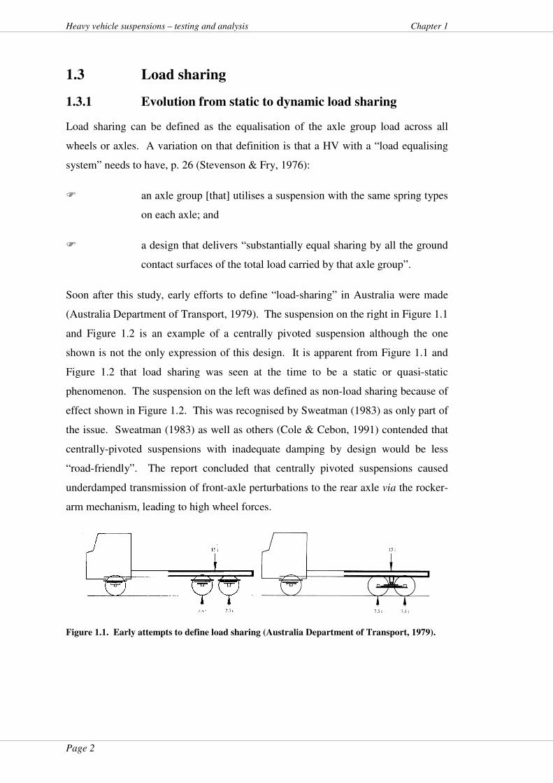
Page 2
Heavy vehicle suspensions – testing and analysis Chapter 1
1.3 Load sharing
1.3.1 Evolution from static to dynamic load sharing
Load sharing can be defined as the equalisation of the axle group load across all
wheels or axles. A variation on that definition is that a HV with a “load equalising
system” needs to have, p. 26 (Stevenson & Fry, 1976):
� an axle group [that] utilises a suspension with the same spring types
on each axle; and
� a design that delivers “substantially equal sharing by all the ground
contact surfaces of the total load carried by that axle group”.
Soon after this study, early efforts to define “load-sharing” in Australia were made
(Australia Department of Transport, 1979). The suspension on the right in Figure 1.1
and Figure 1.2 is an example of a centrally pivoted suspension although the one
shown is not the only expression of this design. It is apparent from Figure 1.1 and
Figure 1.2 that load sharing was seen at the time to be a static or quasi-static
phenomenon. The suspension on the left was defined as non-load sharing because of
effect shown in Figure 1.2. This was recognised by Sweatman (1983) as only part of
the issue. Sweatman (1983) as well as others (Cole & Cebon, 1991) contended that
centrally-pivoted suspensions with inadequate damping by design would be less
“road-friendly”. The report concluded that centrally pivoted suspensions caused
underdamped transmission of front-axle perturbations to the rear axle via the rocker-
arm mechanism, leading to high wheel forces.
Figure 1.1. Early attempts to define load sharing (Australia Department of Transport, 1979).
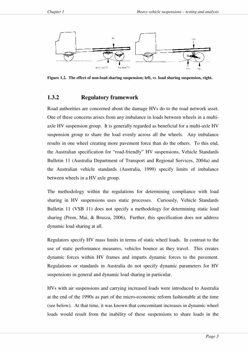
Page 3
Chapter 1 Heavy vehicle suspensions – testing and analysis
Figure 1.2. The effect of non-load sharing suspension; left, vs. load sharing suspension, right.
1.3.2 Regulatory framework
Road authorities are concerned about the damage HVs do to the road network asset.
One of these concerns arises from any imbalance in loads between wheels in a multi-
axle HV suspension group. It is generally regarded as beneficial for a multi-axle HV
suspension group to share the load evenly across all the wheels. Any imbalance
results in one wheel creating more pavement force than do the others. To this end,
the Australian specification for “road-friendly” HV suspensions, Vehicle Standards
Bulletin 11 (Australia Department of Transport and Regional Services, 2004a) and
the Australian vehicle standards (Australia, 1999) specify limits of imbalance
between wheels in a HV axle group.
The methodology within the regulations for determining compliance with load
sharing in HV suspensions uses static processes. Curiously, Vehicle Standards
Bulletin 11 (VSB 11) does not specify a methodology for determining static load
sharing (Prem, Mai, & Brusza, 2006), Further, this specification does not address
dynamic load sharing at all.
Regulators specify HV mass limits in terms of static wheel loads. In contrast to the
use of static performance measures, vehicles bounce as they travel. This creates
dynamic forces within HV frames and imparts dynamic forces to the pavement.
Regulations or standards in Australia do not specify dynamic parameters for HV
suspensions in general and dynamic load sharing in particular.
HVs with air suspensions and carrying increased loads were introduced to Australia
at the end of the 1990s as part of the micro-economic reform fashionable at the time
(see below). At that time, it was known that concomitant increases in dynamic wheel
loads would result from the inability of these suspensions to share loads in the
Page 4
Heavy vehicle suspensions – testing and analysis Chapter 1
dynamic sense. This inability was recognised as having the potential to cause greater
road damage than might otherwise be the case should air-sprung HVs incorporate
more dynamic load equalisation into their design (OECD, 1992, 1998). With the
clarity of hindsight, the disbenefits resulting from heavier air suspended HVs, due to
higher road network asset damage, were probably not recognised as discounting
somewhat the societal and economic benefits of higher payloads.
Three-axle HV semi-trailer groups are commonplace and quad-axle semi-trailers are
being introduced on the Australian eastern seaboard. That air-sprung HV multi-axle
groups do not load share in the dynamic sense has been demonstrated (Davis & Sack,
2004). There is now a growing recognition of the phenomenon of insufficient
dynamic load sharing within air-sprung HV suspension groups. This phenomenon,
particularly for quad-axle semi trailers, is of increasing interest to transport
regulators (Blanksby, George, Peters et al., 2008a; Blanksby, George, Peters et al.,
2008b; Blanksby, Germanchev, Ritzinger et al., 2009).
1.3.3 Dynamic load sharing metrics for HV suspensions
Blanksby (2007) stated that there was no dynamic load sharing measure for HVs.
Others (Patrick, Germanchev, Elischer et al., 2009) have stated that expert opinion
has it that load sharing in the dynamic sense cannot be achieved by current HV
suspension designs (Patrick et al., 2009). Despite this, de Pont (1997) and other
researchers (Cebon, 1999; Potter, Cebon, Collop et al., 1996; Sweatman, 1983) have
been investigating dynamic load sharing of HVs for almost three decades.
Further to the previous work on load sharing, de Pont (1997) developed two dynamic
load sharing metrics but only one, the dynamic load sharing coefficient (DLSC), was
applicable to HV axle groups with more than two axles. It was able to be applied per
wheel or per axle (de Pont, 1997) but not per group without aggregating the results
across wheels or axles.
The most widely used load-sharing measure is the load sharing coefficient (LSC).
This metric is not the most useful and has been criticised since it is really the average
load sharing behaviour of the group (de Pont, 1997). LSC averages the forces on a
Page 5
Chapter 1 Heavy vehicle suspensions – testing and analysis
wheel over a test run and is derived per wheel or per axle. These factors render
difficult a judgement regarding the quality of a HV axle group’s load sharing ability
in totality since six individual and different LSC measures arise from a tri-axle group
test run, for instance. However, little work has been done on replacement for this
metric (de Pont, 1997). Even the DLSC provides a number of different values for
each test run requiring further aggregation to present the data in plain format.
Greater emphasis on, and specification of, the dynamic load sharing ability and other
dynamic parameters of air suspensions is required.
1.3.4 Dynamic load sharing systems
Larger longitudinal air lines on air sprung HVs have been developed (Davis, 2006a,
2007; Davis & Kel, 2007; Willox, 2005). Anecdotal evidence suggests that use of
these systems can improve dynamic load sharing and reduce dynamic forces both
within the HV and transmitted to the pavement via the HV’s wheels. Alterations to
these forces may lead to potential savings in HV suspension designs as well as
savings on structures, surfacings and pavement maintenance. Alterations in these
forces (and the quantum of such alterations) from the use of such systems had not
been determined rigorously until the data for this project were gathered.
Noting that the system tested for this project altered the size of longitudinal air lines
on a HV, side-to-side load sharing is counterproductive to HV handling, resulting in
promotion of roll.
1.3.5 Problem statement # 1
A dynamic load sharing metric without the drawback of aggregating data across
wheels or axles does not exist for axle groups of more than two axles.
Page 6
Heavy vehicle suspensions – testing and analysis Chapter 1
1.3.6 Problem statement # 2
Whether fitting larger longitudinal air lines to air-sprung HVs alters dynamic forces
at the axle-to-body interface has not been determined adequately.
1.4 In-service HV suspension testing
1.4.1 Higher Mass Limits, history and imperatives
The transport industry exerts continuous pressure on road authorities and transport
regulators to allow “freight efficient” vehicles (for which read fewer drivers, more
trailers, more axles and higher axle masses) onto the network.
As part of the micro-economic reform of the 1980s and 1990s the Australian
Government commissioned the mass limits review (MLR) project undertaken by the
National Road Transport Commission (Pearson & Mass Limits Review Steering
Committee, 1996a). The MLR project concluded that HVs operating at higher mass
limits (HML) and equipped with “road friendly” suspensions (RFS) would be no
more damaging to the road network asset than conventional HVs operating at
statutory mass with conventional steel springs (Pearson & Mass Limits Review
Steering Committee, 1996a). Further, the project report stated that HV air
suspensions in poor condition would damage the infrastructure more than HV steel
suspensions and recommended, amongst other things, that eligibility to operate at
HML was dependent on maintenance of dampers. This last point was due to the
heavy reliance air suspensions place on suspension dampers (shock absorbers) for
correct damping. This was in contrast to HV steel suspensions that possess intrinsic
residual damping via the Coulomb friction between the leaves of the steel springs
(Prem, George, & McLean, 1998).
Supported by the findings of the final report of the DIVINE project (OECD, 1998),
the findings of the MLR report led to a reform termed “higher mass limits”
implemented under the “second heavy vehicle reform package” (National Transport
Commission, 2003). Details on the original HML access and conditions when
implemented varied between Australian States and still do. However, in terms of
additional mass, HML generally allowed increases above statutory mass of ∆2.5t on
Page 7
Chapter 1 Heavy vehicle suspensions – testing and analysis
a HV tri-axle group and ∆0.5t on a HV tandem axle group.
In return for HML payloads, HVs carrying them needed to be fitted with RFS that
had been certified as meeting the requirements of VSB 11. This compliance with
VSB 11 was for new suspensions only. VSB 11 was released in 1999 and revised
subsequently (Australia Department of Transport and Regional Services, 2004a,
2004c).
That HVs were permitted to carry greater mass in return for, amongst other
requirements, being equipped with RFS was the first indication that specific axle-
mass increases were to be tied to vehicle design improvements. This approach
signalled to the transport industry there would be minimal scope for any further
blanket increases in gross vehicle mass (GVM). Further, any economic benefits
from increases in GVM were not necessarily going to be balanced against the
increasing costs of maintenance and capital for infrastructure capable of carrying
heavier HVs. It was an acknowledgement that the road network asset had reached a
point where any further gains in HV productivity would need to be traded off against
more efficient boutique vehicles with improved design. That the network would
reach this point had been foreseen (Sweatman, 1994) as well as the prediction of
incentives to encourage HV characteristics which did not consume the asset as
quickly as in the past (Woodrooffe, LeBlanc, & Papagiannakis, 1988).
Interestingly, a decade on from the release of VSB 11, the Austroads guideline for
HV access to local roads (Geoff Anson Consulting & InfraPlan [Aust], 2009) states,
on p. 16: “It is now generally recognised by road authorities that large parts of the
road network infrastructure have reached its capacity in being able to handle heavy
vehicle operation on a general access basis.”
1.4.2 Higher Mass Limits and suspension health
The Mass Limits Review Report and Recommendations by the National Road
Transport Commission (Pearson & Mass Limits Review Steering Committee, 1996a)
found that HV air suspensions in poor condition would damage the infrastructure
more than HV steel suspensions and recommended, amongst other things, that
Page 8
Heavy vehicle suspensions – testing and analysis Chapter 1
eligibility to operate at HML was dependent on maintenance of dampers. Regulators
have become increasingly concerned about this point in recent years.
It is for noting that the only HVs meeting the requirements for RFS in 1999 were air-
suspended although steel suspensions meeting the RFS standard have been released
to the market in the intervening years (Australia Department of Transport and
Regional Services, 2004b).
The DIVINE report showed the results of ineffective shock absorbers on HV wheel
loadings. Figures IV.33 and IV.34 on p. 99 of the DIVINE report, taken from
Woodrooffe (1997), are shown in Figure 1.3. These plots show that, over and above
any static load, when the wheels of a loaded HV were subjected to a 1mm sinusoidal
input, dynamic wheel loads increased by ∆50kN for the case where an air suspension
had ineffective shock absorbers.
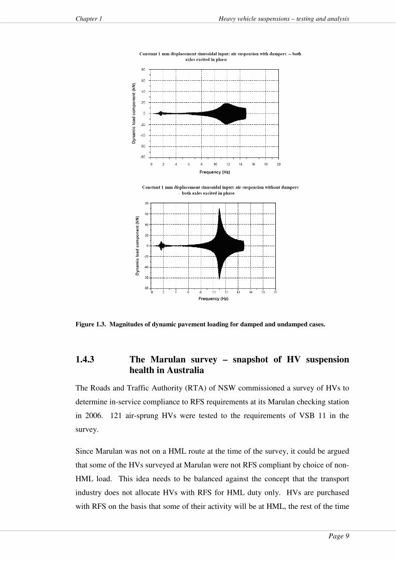
Page 9
Chapter 1 Heavy vehicle suspensions – testing and analysis
Figure 1.3. Magnitudes of dynamic pavement loading for damped and undamped cases.
1.4.3 The Marulan survey – snapshot of HV suspension
health in Australia
The Roads and Traffic Authority (RTA) of NSW commissioned a survey of HVs to
determine in-service compliance to RFS requirements at its Marulan checking station
in 2006. 121 air-sprung HVs were tested to the requirements of VSB 11 in the
survey.
Since Marulan was not on a HML route at the time of the survey, it could be argued
that some of the HVs surveyed at Marulan were not RFS compliant by choice of non-
HML load. This idea needs to be balanced against the concept that the transport
industry does not allocate HVs with RFS for HML duty only. HVs are purchased
with RFS on the basis that some of their activity will be at HML, the rest of the time
Page 10
Heavy vehicle suspensions – testing and analysis Chapter 1
they operate at statutory mass. Unofficial estimates put the number of RFS
suspension sold in Australia per year at 90 percent to 95 percent of the total (Patrick
et al., 2009). Actual figures are difficult to verify since members of the HV
suspension supply industry are reluctant to release official numbers due to the highly
competitive nature of the industry in Australia.
A sample of only 68 HVs with RFS would have provided a 10 percent tolerance level
for the Marulan data (Blanksby, George, Germanchev et al., 2006). Taking the
lowest estimate of RFS-equipped HVs from above, a sample of 121 HVs would have
yielded 108 RFS-equipped HVs; well above the 68 that would have provided a
statistical tolerance level of 10 percent (Blanksby et al., 2006) for the survey result.
From the statistically valid sample of 121 air-sprung HVs, approximately 50 percent
did not meet the damping values specified in VSB 11. Further, 16 percent did not
meet the requirements for frequency values specified in VSB 11. The results from
the Marulan survey indicated strongly that air-sprung HVs were not having their
“road friendliness” maintained during normal work. Dr. Cebon, one of the authors of
the Sweatman et al., (2000) report investigating in-service testing of RFS
suspensions on HVs had already recommended, at the international level, type-
testing of RFS using parametric or other means combined with annual in-service
testing (Cebon, 1999). Others (Potter, Cebon, & Cole, 1997; Woodrooffe, 1995) had
already proposed similar concepts.
In parallel with, but retrospectively encouraged by, the results at Marulan, the States
of Queensland and New South Wales included the development and application of an
in-service HV suspension test in their respective Bilateral Infrastructure Funding
Agreements with the Australian Government (Australia Department of Transport and
Regional Services, 2005a, 2005b).
All Australian State Governments have a Bilateral Infrastructure Funding Agreement
(BIFA) with the Australian Government. These are also known as the “AusLink
agreements”. Each BIFA is an agreement between individual States of Australia and
the Commonwealth and covers arrangements applying to Australian Government
funding to all Australian States under the first five-year AusLink investment
programme (2004-05 to 2008-09) and any agreed modifications thereto. They also
cover actions for infrastructure planning, prioritisation of infrastructure investments
Page 11
Chapter 1 Heavy vehicle suspensions – testing and analysis
opportunities, development and assessment of project proposals and evaluation of
completed projects (Australia Department of Transport and Regional Services,
2005b).
1.4.4 Higher Mass Limits and a “road friendly” suspension
test
In return for extending available HML routes, the States of Queensland and NSW
both agreed with the Commonwealth that an in-service test for “road-friendly” HV
suspensions would be developed and implemented (Australia Department of
Transport and Regional Services, 2005a, 2005b). A project by the National
Transport Commission continues. This thesis and its originating project Heavy
vehicle suspensions – testing and analysis continue to support the National Transport
Commission (NTC) in its endeavours. The road freight industry works to tight
financial margins. Any test for shock absorber health will drive up transport costs.
Accordingly, low cost is beneficial.
1.4.5 Problem statement - in-service HV suspension testing
In Australia at present, there is no:
� requirement to have air-sprung HV air suspensions comply with the
Australian specification for “road-friendly” suspensions, VSB 11
(Australia Department of Transport and Regional Services, 2004a)
once the HV is in service;
� recognised low-cost HV suspension test.
1.5 On-board mass monitoring of HVs
1.5.1 The Intelligent Access Program
Transport Certification Australia Limited (TCA) was created to certify service-
providers of HV telematics and administer the Intelligent Access Program (IAP).
Stage 1 of the IAP monitors HV location, time, speed, tamper-evidence, and
Page 12
Heavy vehicle suspensions – testing and analysis Chapter 1
proprietary trailer identification (Davis, Bunker, & Karl, 2008a).
1.5.2 On-board mass management - program
An alteration to the focus of TCA occurred with respect to on-board mass (OBM)
monitoring. As mentioned in Section 1.4.4, the funding arrangements between the
Australian Government and the various State Governments are covered, in part, by
each State’s BIFA. The BIFAs for NSW and Queensland from 2004-05 to 2008-09
(Australia Department of Transport and Regional Services, 2005a, 2005b) included
obligations requiring HML vehicles to be monitored by the IAP for position and,
importantly for this thesis, on-board mass monitoring.
1.5.3 On-board mass monitoring
TCA, jointly with the NTC, has undertaken a project to investigate the feasibility of
on-board vehicle mass-monitoring devices to be incorporated into Stage 2 of the IAP
(Davis et al., 2008a). On-board mass monitoring (OBM) increases jurisdictional
confidence in operational HV compliance. This research project has identified
technical issues regarding on-board mass monitoring systems including:
� determination of HV mass using OBM systems at an evidentiary
level (i.e. accurate enough to be used as evidence in a prosecution);
� accuracy, robustness and tamper issues of OBM components (mass
sensors, connections, power supply, display unit etc.); and
� potential use of dynamic data to cross check measurement results
from OBM systems.
Page 13
Chapter 1 Heavy vehicle suspensions – testing and analysis
1.5.4 Problem statement – on-board mass monitoring of
HVs
Tamper-evidence and accuracy of current OBM systems needed to be determined
before any regulatory schemes were put in place for its use. There are no regulatory
on-board mass schemes for HVs operating anywhere in the world. Australia, via the
Intelligent Access Programme (Davis et al., 2008a; Karl, 2007; Karl, Davis, Cai et
al., 2009; Transport Certification Australia, 2005) is examining the feasibility of
such implementation.
1.6 Research aims
The following Research Aims have been developed from the problem identification
in Sections 1.3 to 1.5.
1.6.1 Aim 1: Dynamic load sharing 1
Hypothesis:
“An improved dynamic load sharing measure can be developed for heavy vehicle
suspensions.”
The research aimed to test this hypothesis by:
� examining the existing load sharing measures available for heavy
vehicles;
� determining whether these are suitable and; if not
� developing a dynamic load sharing parametric measure (or
measures) that can be applied to consecutive wheels or axles.
Page 14
Heavy vehicle suspensions – testing and analysis Chapter 1
1.6.2 Aim 2: Dynamic load sharing 2
Hypothesis:
“Alterations to dynamic parameters, particularly dynamic load sharing, occur from
the use of larger longitudinal air lines in air-suspended HVs.”
The research project aimed to:
� determine if larger air lines on air sprung HVs make a difference to
wheel force parameters and axle-to-body force parameters and, if
so;
� determine the quantum of such alterations to wheel forces and axle-
to-body forces from the use of larger longitudinal air lines.
1.6.3 Aim 3: In-service HV suspension testing
Hypothesis:
“A low-cost in-service suspension test for HVs is possible.”
The research project aimed to explore low-cost methods to evaluate
� if equivalent outcomes to VSB 11 testing for body bounce and
damping ratio may be achieved. This for validity, via “proof-of-
concept” of the “pipe test” (Davis & Bunker, 2008a) consisting of
driving the HV over a 50mm steel pipe and analysing the body
bounce and damping; and
� the development of a modified brake tester to impart resonant forces
into HV suspensions.
The latter would be used to:
� compare previous work on wheel forces from suspensions in good
condition vs. those equipped with poor/worn shock absorbers, such
as in the lower window of Figure 1.3, after Woodrooffe (1997); and
Page 15
Chapter 1 Heavy vehicle suspensions – testing and analysis
� determine a “proof-of-concept” for a second, low-cost HV
suspension tester to inform the NTC project referenced above.
1.6.4 Aim 4: On-board mass monitoring of HVs – search for
accuracy and tamper-evidence
Hypothesis:
“On-board mass measurement systems for HVs are accurate and tamper-evident for
Australian regulatory purposes.”
The research project aimed to determine:
� the accuracy of currently-available on-board mass (OBM) systems
by analysis of weighbridge vs. OBM reading;
� the use of dynamic data from OBM systems to detect tamper events;
and
� whether dynamic data from OBM systems could be used to derive
static HV mass.
1.7 Objectives
A programme was established to address the Research Aims in Section 1.6 to meet
the following objectives.
1.7.1 Objective 1 – dynamic load sharing metric
Develop at least one dynamic load sharing parametric measure that can be applied to
the axle group, consecutive axles or to consecutive wheels and for more than two
axles.
Page 16
Heavy vehicle suspensions – testing and analysis Chapter 1
1.7.2 Objective 2 – differences for larger longitudinal air
lines
Determine if larger air lines on air sprung HVs make a difference to wheel forces and
axle-to-body forces and, if so, determine the quantum of such alterations from the
use of larger longitudinal air lines.
1.7.3 Objective 3 – development of in-service suspension
test(s)
Explore low-cost HV suspension test methods. Evaluate if low-cost HV suspension
test methods can be made equivalent to VSB 11 outcomes for body bounce and
damping ratio. Evaluate the validity, via “proof-of-concept” of the “pipe test” (Davis
& Bunker, 2008e). Develop a modified roller-brake tester to impart resonant forces
into a HV suspension and, in part, validate previous work on wheel forces from
suspensions in good condition vs. those equipped with poor/worn shock absorbers
(Woodrooffe, 1997). Determine, via “proof-of-concept”, that a modified roller-brake
tester may be used to detect a worn HV suspension compared with one within
specification. This latter to inform the NTC project referenced above.
1.7.4 Objective 4 – on-board mass measurement feasibility
Determine the accuracy of currently-available OBM systems. Examine the accuracy
of OBM readings vs. weighbridge readings. Validate the use of dynamic data from
OBM systems to detect tamper events.
Page 17
Chapter 1 Heavy vehicle suspensions – testing and analysis
1.8 Scope, definitions, conventions and limitations
of the study
1.8.1 Glossary, terms, acronyms and abbreviations
Terms,
abbreviations
and acronyms
Meaning
AASHO American Association of State Highway Officials. Became AASHTO.
AASHTO American Association of State Highway and Transportation Officials.
ALF Accelerated loading facility.
APT Air pressure transducer. A device that converts an air pressure signal to a
proportional electrical signal.
ARRB Australian Road Research Board – now privatised, has changed its name to
ARRB Group Limited.
ARRB Australasian Road Research Board.
ARTSA Australian Road Transport Suppliers Association.
ATC Australian Transport Council. “The Australian Transport Council (ATC) is
a Ministerial forum for Commonwealth, State and Territory consultations
and provides advice to governments on the coordination and integration of
all transport and road policy issues at a national level.”
http://www.atcouncil.gov.au.
ATRF Australasian Transport Research Forum. A conference for presentation of
papers and colloquia on matters of transport planning, policy and research.
Axle-hop Vertical displacement of the wheels (and axle), indicating dynamic behaviour of the axle and resulting in more or less tyre force onto the road. Usually manifests in the frequency range 10 – 15Hz.
BIFA Bilateral Infrastructure Funding Agreement. Also known as “AusLink agreement”. An agreement between individual States of Australia and the Commonwealth which “covers arrangements applying to funding made available by the Australian Government to Queensland under the first five-year AusLink investment programme (2004-05 to 2008-09) and any agreed subsequent changes to, and extensions of, the programme. It also covers agreed arrangements for infrastructure planning, identification of investment priorities, development and assessment of project proposals and evaluation of completed projects.” (Australia Department of Transport and Regional Services, 2005b). Queensland’s BIFA may be viewed at: http://www.auslink.gov.au/publications/policies/pdf/Queensland_bilateral.pdf.
Page 18
Heavy vehicle suspensions – testing and analysis Chapter 1
Body bounce Movement of the sprung mass of a truck as measured between the axles and the chassis. Results in truck body dynamic forces being transmitted to the road via the axles & wheels. Usually manifests in the frequency range 1 – 4Hz.
CAPTIF Canterbury Accelerated Pavement Testing Indoor Facility.
CoG Centre of gravity. The point at which a body’s mass may be said be concentrated for purposes of determining forces on that body.
∆ Greek letter “delta” – denoting increment.
Damping ratio
How rapidly a dynamic reduces impulsive response. It is found from the ratio of the peak of one dynamic cycle to the peak in the next cycle. The
damping ratio, zeta )(ζ is given as a value under 1 (e.g. 0.3) or a
percentage (e.g. 30 percent).
DIF Dynamic impact factor (Woodrooffe & LeBlanc, 1987). See also PDWF & PDLR.
DIVINE The Dynamic Interaction between Vehicles and Infrastructure Experiment. The Dynamic Interaction between Vehicles and Infrastructure Experiment (DIVINE) Project was formulated to report on dynamic effects of heavy vehicles on infrastructure to inform transport policy decisions regarding that infrastructure and road transport costs.
DLC Dynamic load coefficient (Sweatman, 1983).
DLSC Dynamic load sharing coefficient (de Pont, 1997).
Dot operator Denotes derivative with respect to time. Where (say) x is a time-dependent
variable, dt
dx denotes the derivative or the rate of change with respect to
time. This concept is sometimes designated x& as a shortened form. The
derivative with respect to time of x& , that is 2
2
dtxd or acceleration, is
designated x&& .
DoTaRS Department of Transport and Regional Services. An Australian Government department.
DTMR Department of Transport and Main Roads. Queensland Government Department formed from the amalgamation of the Departments of Main Roads and Queensland Transport in March 2009.
Eigenfrequency Frequency of a body at one of its vibrational resonance modes.
ESA Equivalent standard axle.
EU European Union.
FFT Fast Fourier transform. A method whereby the Fourier transform is found using discretisation and conversion into a frequency spectrum (see Fourier transform).
Page 19
Chapter 1 Heavy vehicle suspensions – testing and analysis
Fourier transform
A method whereby the relative magnitudes of the frequency components of a time-series signal are converted to, and displayed as, a frequency series (Jacob & Dolcemascolo, 1998).
GVM Gross vehicle mass.
HML Higher Mass Limits. Under the HML schemes in Australia, heavy vehicles are allowed to carry more mass (payload) in return for their suspension configuration being “road friendly”. See VSB 11.
HV Heavy vehicle.
Hz Hertz. Unit of vibration denoting cycles per second. Units are s-1.
IRI International roughness index.
LSC Load sharing coefficient. A measure of how well a suspension group equalises the total axle group load, averaged during a test. This is a value which shows how well the average forces of a multi-axle group are distributed over each tyre &/or wheel in that group (Potter et al., 1996).
MCV Multi-combination vehicle. HVs with general arrangement or GVM greater than that of a semi-trailer.
MLR Mass Limits Review. The national project that resulted in the implementation of HML in Australia.
NHVAS National Heavy Vehicle Accreditation Scheme. A voluntary scheme that certifies transport operators against a set of industry-specific quality assurance requirements. Membership of this scheme is a pre-requisite for HML.
NRTC National Road Transport Commission. A national body set up by the States of Australia to facilitate economic reform of the road transport industry. Became the NTC earlier this decade.
NSW New South Wales.
NTC See NRTC.
OECD Organisation for Economic Co-operation and Development.
OBM On-board mass. Systems for measuring the mass of a heavy vehicle using on-vehicle telematics.
PDF Peak dynamic force.
PDLR Peak Dynamic Load Ratio (Fletcher, Prem, & Heywood, 2002).
PDWF Peak dynamic wheel force. The maximum wheel force experienced by a wheel during dynamic loading as a result of a step input (Fletcher et al., 2002). If applied to axle forces, this measure is related to dynamic impact factor (DIF) as the numerator in the equation.
PSD Power spectral density.
Page 20
Heavy vehicle suspensions – testing and analysis Chapter 1
QUT Queensland University of Technology.
RFS “Road-friendly” suspension. A HV suspension conforming to the performance requirements defined by VSB 11.
http://www.dotars.gov.au/roads/safety/bulletin/pdf/vsb_11.pdf
RSF Road stress factor. An estimation of road damage due to the 4th power of instantaneous wheel force (Potter et al., 1997).
RTA Roads and Traffic Authority (NSW).
Shock absorber See suspension damper.
Sigma (σ) Greek symbol lower-case ‘sigma’, denoting standard deviation.
Spatial repeatability
The tendency for HV suspensions with similar characteristics to concentrate wheel forces at particular points on any given length of road.
Suspension damper
A device used to provide vibration damping to the suspension of a vehicle. This device reduces perturbations in suspension travel over time. It damps out axle-hop; contributes to tyre contact with the pavement during travel over undulations and during braking.
TCA Transport Certification Australia.
TMR See DTMR.
VSB 11 Vehicle Standards Bulletin 11. A document issued by DoTaRS that defines the performance parameters of “road-friendly” HV suspensions.
WiM Weigh-in-motion. Technology that uses sensors in the road to measure the wheel force of vehicles.
Page 21
Chapter 1 Heavy vehicle suspensions – testing and analysis
1.8.2 Scope
The scope of the project was limited to measurement of data at the wheels and the
springs of heavy vehicles. This was to:
� develop low-cost methods for in-service testing of HV suspensions
as alternatives to the method defined in the Australian specification
for “road friendly” suspensions Vehicle Standards Bulletin 11 (VSB
11);
� determine whether larger longitudinal air lines fitted to HV air
spring suspensions altered forces at the springs or the wheels and, if
so, by how much;
� derive frequency-series data from the testing to inform the activities
of the project;
� develop HV suspension models to support the above activities and
alter their parameters to determine areas for future HV suspension
development;
� determine the accuracy and precision of on-board mass (OBM)
telematics for HVs; and
� determine whether a tamper indicator could be developed for OBM
systems for HVs.
The study considered legal (statutory mass and HML) heavy vehicle loads. Road
network damage due to overloading was not part of the study parameters.
1.8.3 Numbering convention
In general, numbers have been shown to three significant figures. In places where
this has not occurred, it was due to the derived values being sensitive to the least
(usually fourth) significant figure or where mass could be measured to 0.1 kg.

Page 22
Heavy vehicle suspensions – testing and analysis Chapter 1
1.9 Outline of the research methodology
1.9.1 The scientific method
The standard experimental methodology of performing a test with a known or
standard system, changing one feature, running the experiment again and then
comparing the two sets of data was performed. Thus the standard scientific method
where the results from a control case were compared with those from a test case
(Mill, 1872) was implemented for the experimental design and the analysis of the
data.
1.9.2 Dynamic load sharing metric
Currently available load sharing metrics were reviewed. By deriving suspension
metrics from the data collected during the testing (Davis & Bunker, 2008e), it was
apparent that a dynamic load sharing parameter using instantaneous data was
available. This was developed further and the results documented.
1.9.3 Differences for larger longitudinal air lines
Three air-suspended HVs were instrumented to measure air spring and wheel forces
during typical travel. Two sets of tests were conducted. The control case had
standard air lines and the test case was for larger longitudinal air lines between the
air springs. Suspension parameters for load sharing and dynamic forces were
derived. By comparing these for the test case vs. the control case, conclusions were
drawn. Using the suspension parameters derived from a combination of
manufacturer’s data and observed behaviour during other testing (Section 1.9.4), the
fundamental parameters of the HV suspension were determined. This allowed a
computer model of a theoretical HV suspension to be created. By varying the load-
sharing ability of this model, further improvements in HV suspension design were
apparent. These were documented but not developed as this line of research was
tending out-of-scope.
Page 23
Chapter 1 Heavy vehicle suspensions – testing and analysis
1.9.4 Development of in-service suspension test(s)
Method 1. Using the testing of three HVs described above, a novel suspension test,
the “pipe test” was performed. The control test was a replication of the step-down
test in the Australian specification for “road-friendly” suspensions, VSB 11. The
results from the novel test were compared with those from the VSB 11 test.
Method 2. A used FKI Crypton HV brake tester (FKI Crypton Ltd, 1990) was
modified and instrumented. A test HV wheel was excited by two flat areas on the
roller when it was spun up to speed. Instrumentation measured the wheel forces thus
created. Dampers with differing levels of wear were fitted. The control case was for
a new shock absorber, the two test cases were for a damper worn to the point where
tyre degradation was occurring and the other test case was for no shock absorber.
The wheel forces were analysed for magnitude and frequency for the cases tested.
Threshold values for shock absorber wear vs. wheel forces were determined as a
“proof-of-concept” in-service HV suspension test. This informed the NTC project
and assisted in proposing low-cost HV air-suspension test methods.
1.9.5 On-board mass feasibility
The testing program was conducted in line with Davis et al. (Davis et al., 2008a;
Davis, Bunker, & Karl, 2008b). Twelve test and control OBM systems from eight
suppliers were installed on eleven HVs. The HVs were loaded to tare, 1/3, 2/3 and
full load points. The HVs were then weighed six times per load point on
weighbridges after a short road circuit. Dynamic data were recorded for the road
circuits. The weighbridge readings were compared with the static OBM readings. A
range of dynamic data was recorded as the test vehicles encountered speed bumps,
braking and cornering.
Tests were performed to determine potential for, and ease of, tampering. Various
tamper tests were performed; the one that concerns this thesis directly was that where
the air lines to the OBM primary transducer were closed off. Dynamic data were
recorded for open and closed air line states. The two sets of data were compared and
an algorithm developed to detect the difference.
Page 24
Heavy vehicle suspensions – testing and analysis Chapter 1
1.10 Structure of the thesis
This thesis is structured in chapters. The chapter numbers and their titles are as
shown in the diagram, Figure 1.4. The diagram defines the interconnections and
precedent/outcome succession within the methodology used to achieve the
objectives, described above.
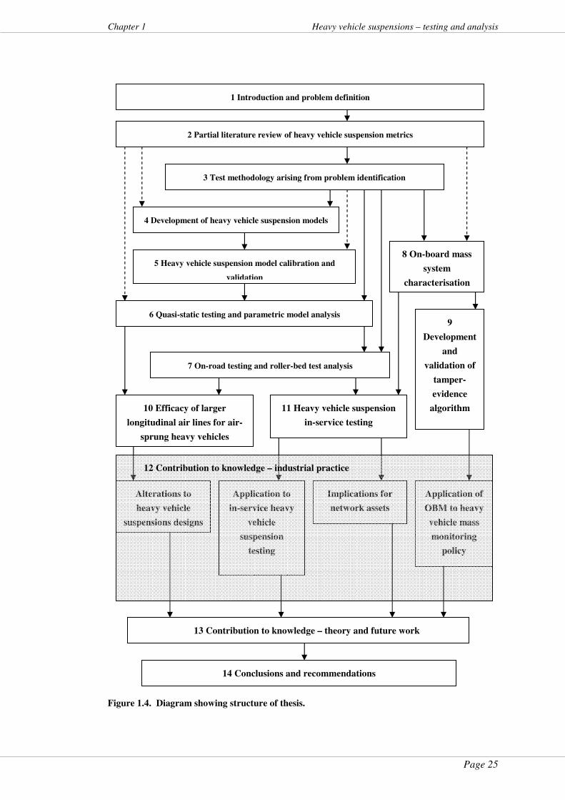
Page 25
Chapter 1 Heavy vehicle suspensions – testing and analysis
Figure 1.4. Diagram showing structure of thesis.
2 Partial literature review of heavy vehicle suspension metrics
4 Development of heavy vehicle suspension models
8 On-board mass
system
characterisation
5 Heavy vehicle suspension model calibration and
validation
14 Conclusions and recommendations
9
Development
and
validation of
tamper-
evidence
algorithm 11 Heavy vehicle suspension
in-service testing
Application of
OBM to heavy
vehicle mass
monitoring
policy
Alterations to
heavy vehicle
suspensions designs
Application to
in-service heavy
vehicle
suspension
testing
10 Efficacy of larger
longitudinal air lines for air-
sprung heavy vehicles
6 Quasi-static testing and parametric model analysis
Implications for
network assets
12 Contribution to knowledge – industrial practice
13 Contribution to knowledge – theory and future work
7 On-road testing and roller-bed test analysis
1 Introduction and problem definition
3 Test methodology arising from problem identification
Page 26
Heavy vehicle suspensions – testing and analysis Chapter 1
1. Introduction and problem definition (this chapter) sets the scene for the
thesis. It describes the aims, objectives, background, limitations and scope of
the project. Definitions, abbreviations and acronyms are set out.
2. Review of heavy vehicle suspension metrics contains a summary of
measures and parameters used by regulators, researchers and the heavy
vehicle industry in their attempts to quantify the relative values of HV
suspensions.
3. Data collection documents the test programme methodology used to gather
the data for the project.
4. Development of heavy vehicle suspension models covers the process where
HV suspensions were conceptualised and then models assembled for use in
the project.
5. Heavy vehicle suspension model calibration and validation applies the
data gathered for the project to the concept models developed in the previous
chapter. This to calibrate and validate the HV suspension models.
6. Quasi-static testing provides results from the quasi-static test programme. It
also uses the models developed, calibrated and validated in the previous
chapters. This to determine some metrics for the suspensions tested.
7. On-road testing and roller bed test analysis provides results from the
roller-bed testing and the on road test programme, save for the OBM testing.
It also details the development of an innovative metric relating to roughness.
This is then used to illustrate wheel loadings and discuss pavement damage
model parameters.
8. On-board mass system characterisation describes the accuracy, precision
and other characteristics determined from testing of OBM systems.
9. Development and validation of a tamper metric provides the rationale for,
and subsequent development and validation of, an indicator of tampering with
on-board mass (OBM) telematics systems where the air lines to the air-
pressure transducers have been restricted.
10. Efficacy of larger longitudinal air lines details derived measures from the
testing of the control case of standard air lines vs. larger longitudinal air lines.
Further, it details a novel dynamic load sharing test.
Page 27
Chapter 1 Heavy vehicle suspensions – testing and analysis
11. HV suspension in-service testing discusses how various testing methods,
particularly low-cost ones, may be applied to in-service testing of HV
suspensions and the implications of this approach within a regulatory
framework.
12. Contribution to knowledge – industrial practice details the contribution to
knowledge, from this project, that is readily applicable to industrial practice.
It is in four Sections:
� Alterations to HV suspensions explores the possibilities discovered
during the analysis of the different HV suspension types and
configurations. Further, by varying the internal parameters of the
models developed in Chapters 4 and 5, theoretical improvements are
mooted for novel suspension configurations.
� Application of in-service HV suspension testing provides a
framework for applying the in-service suspension tests developed
earlier.
� Implications for network assets discusses the issues related to poor
HV suspension performance if allowed to deteriorate from the new
state.
� Application of OBM to HV monitoring policy explores the
possibilities of OBM as a regulatory tool.
13. Contribution to knowledge – theory and future work details the
contribution to theoretical knowledge from this project. It also provides
suggestions to researchers who may wish to develop some of the concepts
explored in this thesis in academic, theoretical or abstract variable-space in
the future.
14. Conclusions and recommendations summarises the work and how the
objectives were met.
Page 28
Heavy vehicle suspensions – testing and analysis Chapter 2
2 Partial literature review of heavy vehicle
suspension metrics
2.1 About this chapter
The purpose of this chapter is to summarise the suspension metrics used later in this
thesis. It is not exhaustive and the interested reader is referred to the literature
review (Davis & Bunker, 2007) for more information.
This chapter presents novel work on load sharing from the project and sets the scene
for the development of models with respect to dynamic load sharing, suspension
design and road damage.
2.2 Introduction to this review
This review is presented in three parts; one part relating to temporal measures, the
second concerning spatial measures and the third presenting a study into the load
sharing coefficient (LSC) and its relationship to dynamic load coefficient (DLC).
New material developed since the literature review of this project (Davis & Bunker,
2007) is included, noting particularly the spatial correlation work outlined in Section
2.4.5 (Blanksby, Germanchev, Ritzinger et al., 2009) and the study of DLS vs. LSC
(Davis & Bunker, 2009d) in Section 2.5.
The split between the first two sections reflects the two major research philosophies
regarding heavy vehicle (HV) dynamics and their impact on pavements. The
temporal approach (section 2.3) tends to see HV dynamics in terms of inter-axle or
inter-wheel interactions. The spatial approach (section 2.4) views dynamic forces
from HVs in terms of their wheel forces passing a point on the road, particularly
where homogeneity of suspension types or specifications increases the probability of
wheel force repetition at a particular point of the pavement. Such forces are
generated by dynamic response due to a defect in the pavement at some previous
point or from axle-hop due to defective dampers. Australian research in the spatial
metric domain has had an addition since the literature review for this project was
completed. This work is reviewed in Section 2.4.5.
Road asset owners are primarily concerned with pavement damage caused by HVs.
Page 29
Chapter 2 Heavy vehicle suspensions – testing and analysis
Subtleties of suspension design are not the intrinsic focus of this approach but are a
means to minimise asset degradation. Accordingly, pavement damage models as
they relate to HV suspension designs and metrics are covered in this chapter to the
extent that they are related.
2.3 Temporal measures
The following measures for HV suspensions are designated ‘temporal’ (Cebon,
1987) since they are dependent on the forces on the chassis or wheels within a
particular history.
2.3.1 Damping ratio
The damping ratio in the context of a HV suspension is a measure of how quickly a
HV body returns to steady state motion after encountering a bump in the road.
Damping ratio is designated by the Greek letter zeta (ζ), is dimensionless and usually
shown as a number less than 1.0 (e.g. 0.3) or as a percentage (e.g. 30 percent)
denoting the damping present in the system as a fraction of the critical damping
value (Doebelin, 1980).
Apart from other specified parametric thresholds, HV “road friendly” suspensions
are required to have:
� a damping ratio, zeta (ζ), of greater than 0.2 or 20 percent with
dampers fitted; and
� a contribution of more than 50 percent to the overall viscous
damping value of the measured damping ratio from the dampers
(Australia Department of Transport and Regional Services,
2004a).
Page 30
Heavy vehicle suspensions – testing and analysis Chapter 2
2.3.2 Damped natural frequency
The damped natural frequency of the sprung mass (body), in the HV suspension
environment, is the measure of how many times per second the HV body bounces
after some perturbation (e.g. bump in the pavement).
For a HV suspension to be defined as “road-friendly”, not only does the damping
ratio have to exceed certain values (above), but also the damped free vibration
frequency (f) of body bounce needs to be less than 2.0 Hz.
Davis and Sack (Davis & Sack, 2004, 2006) as well as Sweatman (Sweatman, 1983)
have shown the magnitude of parameters of interest (including body bounce but also
axle-hop, etc.) either as a frequency series using the output of a fast-Fourier
transform (FFT) or as a power spectral density (PSD) against frequency (Gyenes &
Simmons, 1994; Jacob & Dolcemascolo, 1998; LeBlanc & Woodrooffe, 1995;
OECD, 1998). Essentially, the two methods (PSD vs. FFT) do not differ in their
application to finding resonant frequencies. The vertical scales differ between the
two methods in that the vertical axis of the PSD graph is proportional to the square of
the magnitude of the FFT graph (Vernotte, 1999).
2.3.3 Digital sampling of dynamic data – Shannon’s theorem
(Nyquist criterion)
Following from the previous section on frequency and to inform the rationale behind
data sampling choices detailed later in this thesis (Chapter 3), an expansion on digital
sampling theory follows (Davis & Bunker, 2007).
In order to re-create a signal with frequency components from 0 Hz to fi Hz, where fi
Hz is the maximum frequency of interest, the Shannon-Nyquist sampling theorem
states that the sampling rate, fs, must be a minimum of if×2 Hz (Considine, 1985).
Noting that frequency, ω, in radians is related to conventional frequency f in Hz by:
ω = 2πf
Equation 2.1
Page 31
Chapter 2 Heavy vehicle suspensions – testing and analysis
then the following proof may be considered.
Let T be the system sampling time in seconds (s) of a continuous time-series signal
where the highest frequency of interest in the sampled signal is ωi rad.s-1 and θ is
the phase angle. The continuous time-series signal may be represented by:
)sin()( θω += tte i
Equation 2.2
Let the sampling frequency in radians be ωs, where 0 < ωi < ωs /2.
The sampling frequency, ωs, relates to conventional sampling frequency, fs, in Hz by:
2πfs = ωs = 2π/T.
=> T = 2π/ωs
Equation 2.3
Let t = kT where k is a constant.
Substituting kT for t in Equation 2.2, the equation for the sampled signal may be
represented:
=> )sin()( θω += TkkTe i
Equation 2.4
Now consider a different continuous time-series signal with higher frequencies
where the higher frequencies contain a component nωs in addition to ωs and
represented by:
[ ]θωω ++= tntf si )(sin)(
Equation 2.5
where n = 1, 2, 3…
Substituting 2π/T for ωs from Equation 2.3, Equation 2.5 becomes:
+
××+= θ
πω t
T
ntf i )
2(sin)(
Equation 2.6
Page 32
Heavy vehicle suspensions – testing and analysis Chapter 2
for which the sampling time T is as above.
Substituting kT for t as before, the equation for the reconstructed signal is then:
+
××+= θ
πω kT
T
nkTf i )
2(sin)(
=> )sin()( θω += ikTkTf
Equation 2.7
As the signal frequencies in Equation 2.6 increase proportional to 2π/T, the
reconstructed signal in Equation 2.7 becomes indistinguishable from Equation 2.4,
even though the frequency of the signal has been increased.
Hence, ωi < ωs/2 is the criterion for the process of regular time-based sampling. At
the limit, as ωi approaches nωs /2, or:
ωi lim nωs /2
the reconstruction process for sampled signals is unable to make the distinction
between any two sampled signals for all cases of integer values of n.
Beyond this limit, where ωi > ωs /2, the reconstructed frequencies are “folded” back
into the frequency spectrum interval 0 < ωi < ωs/2 and it becomes impossible to
reconstruct ωi frequencies greater than ωs /2 from the sampled signal.
The critical sampling frequency π/T is often referred to as the “Nyquist frequency”.
The selection of small enough values of T to achieve valid reconstruction of signals
is termed Shannon’s theorem, which may be stated as either of the following two
imperatives:
ωs > 2 ωi
or
π/T > ωi
(Houpis & Lamont, 1985).
Page 33
Chapter 2 Heavy vehicle suspensions – testing and analysis
2.3.4 Dynamic load coefficient
Sweatman (1983) developed a measure designated the dynamic load coefficient
(DLC) in his work “A study of dynamic wheel forces in axle group suspensions of
heavy vehicles. Special Report No. 27” (Sweatman, 1983). This was, in part, based
on earlier work (Sweatman, 1980) and was to account for, and allow comparison
between, the relative effects of dynamic wheel force behaviour of differing
suspension types.
The DLC was defined as the coefficient of variation of dynamic wheel forces relative
to the static wheel force; i.e. the ratio of variation in dynamic wheel forces to static
wheel force. That approach utilised the concept that a measure of road damage could
incorporate a damage component due to:
� dynamic forces present from wheel loads; plus
� a component due to the static forces present.
The static wheel force was represented in this measure by the “mean wheel load”
Fmean (Figure 2.1). The dynamic forces were represented in this measure as the
standard deviation (σ) or root-mean-square (RMS) of the dynamic wheel force
(Figure 2.1).
The DLC may be defined mathematically:
DLC = σ / Fmean
Equation 2.8
where:
σ = the standard deviation of wheel force; and
Fmean = the mean wheel force (Sweatman, 1983).
It assumes that:
� dynamic loads are random and have a Gaussian distribution about
Fmean as shown in Figure 2.1, after DIVINE (OECD, 1998); and
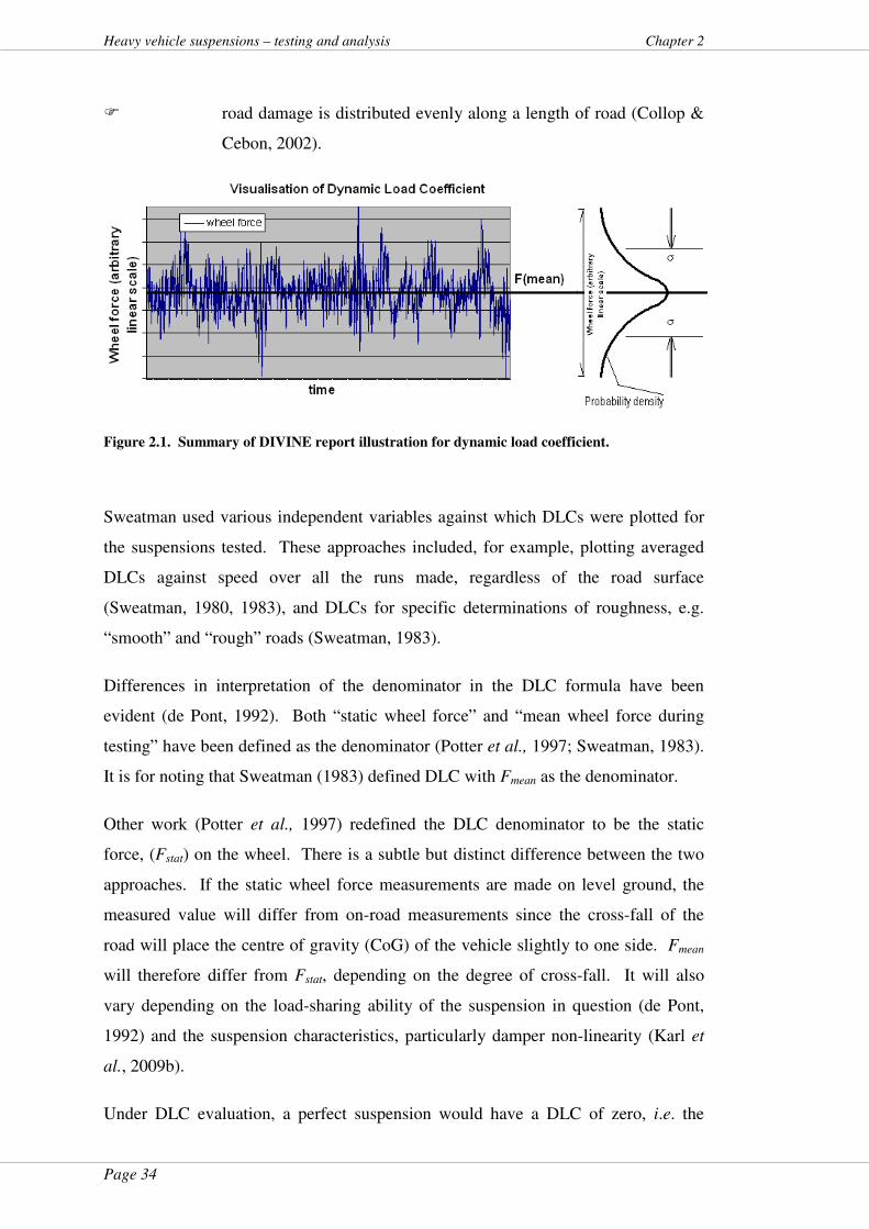
Page 34
Heavy vehicle suspensions – testing and analysis Chapter 2
� road damage is distributed evenly along a length of road (Collop &
Cebon, 2002).
Figure 2.1. Summary of DIVINE report illustration for dynamic load coefficient.
Sweatman used various independent variables against which DLCs were plotted for
the suspensions tested. These approaches included, for example, plotting averaged
DLCs against speed over all the runs made, regardless of the road surface
(Sweatman, 1980, 1983), and DLCs for specific determinations of roughness, e.g.
“smooth” and “rough” roads (Sweatman, 1983).
Differences in interpretation of the denominator in the DLC formula have been
evident (de Pont, 1992). Both “static wheel force” and “mean wheel force during
testing” have been defined as the denominator (Potter et al., 1997; Sweatman, 1983).
It is for noting that Sweatman (1983) defined DLC with Fmean as the denominator.
Other work (Potter et al., 1997) redefined the DLC denominator to be the static
force, (Fstat) on the wheel. There is a subtle but distinct difference between the two
approaches. If the static wheel force measurements are made on level ground, the
measured value will differ from on-road measurements since the cross-fall of the
road will place the centre of gravity (CoG) of the vehicle slightly to one side. Fmean
will therefore differ from Fstat, depending on the degree of cross-fall. It will also
vary depending on the load-sharing ability of the suspension in question (de Pont,
1992) and the suspension characteristics, particularly damper non-linearity (Karl et
al., 2009b).
Under DLC evaluation, a perfect suspension would have a DLC of zero, i.e. the
Page 35
Chapter 2 Heavy vehicle suspensions – testing and analysis
wheel force would not vary above or below the static value. The range, in reality, is
somewhere between 0 and 0.4 (Mitchell & Gyenes, 1989). Many researchers
(Gyenes, Mitchell, & Phillips, 1992; Mitchell & Gyenes, 1989) have used DLC as
one measure to differentiate suspension types from each another (e.g. steel vs. air).
Despite this, the use of DLC has been criticised for purposes of attempting to
distinguish between the damage potential of suspensions with different axle groups
(Potter et al., 1996) and despite being adopted as the de-facto standard as a road-
damage determinant (OECD, 1998).
DLC continues to be criticized, most recently by Dr. Cebon at the Fifth Brazilian
Congress on Roads and Concessions; along the line of: “how this [DLC] method
leads to false conclusions regarding where and how to use road maintenance funds,
spatial repeatability of road surface stress being the key issue.” (Lundström, 2007).
This criticism is not new (Cebon, 1987). DLC shares a drawback with other
suspension parameters that derive a value per wheel or per axle; the need to
aggregate or average the different DLC values per axle or wheel to get a manageable
picture of it against independent variables or for comparison of differing suspension
designs.
2.3.5 Load sharing coefficient
Early attempts to determine load sharing of HV suspensions (Sweatman, 1976) were
by driving a test HV over a 40mm plank and measuring the load under the plank.
Changes in axle loads, during the dynamic load conditions created thereby, were then
compared with static loads.
Sweatman (1983) attempted to quantify the load sharing ability of a multi-axle group
in a number of ways, amongst which was the load sharing coefficient (LSC). This
was designed to be a measure of how a suspension group shared the total axle group
load across the axles within the group. It is a value of the ability of a multi-axle
group to distribute its load over each tyre and/or wheel in that group during travel.
Page 36
Heavy vehicle suspensions – testing and analysis Chapter 2
The original definition of LSC was:
t)group (sta
mean
F
Fn LSC
××=
2
Equation 2.9
where:
n = number of axles in the group;
Fgroup (stat) = axle group static force and
Fmean = the mean wheel force in Figure 2.1 (Sweatman, 1983).
Note that this approach treated the load sharing as being between axles.
Sweatman (1980) stated that the net increase in road damage, ∆damage, due to unequal
loading of (say) 10 percent between axles in a tandem group assuming, again, the
‘fourth-power law’, may be calculated by:
∆damage = 0.5 x [1.14 + 0.94 – (1+1)] x 100%
Equation 2.10
This approach did not necessarily agree with other, early definitions such as that of
Stevenson & Fry (1976) p. 24, that a HV with a “load equalising system” meant that
an axle group utilised a suspension with the same spring types on each axle and that
this resulted in “substantially equal sharing by all the ground contact surfaces of the
total load carried by that axle group”. Note the emphasis on wheel forces in the
context of “ground contact surfaces”, not axle forces.
LSC has been simplified and modified more recently to:
stat (nom)
mean
F
(i)FLSC =
Equation 2.11
where:
Fstat (nom) = Nominal static tyre force =n
F al)group (tot;
Fgroup (total) = Total axle group force;

Page 37
Chapter 2 Heavy vehicle suspensions – testing and analysis
Fmean (i) = the mean force on tyre/wheel i; and
n = number of tyres in the group (Potter et al., 1996).
Equation 2.9 and Equation 2.11 differ in that the latter focuses on the equalisation of
wheel forces and the former on equalisation of axle forces. This may be attributed to
a difference in interpretation between schools of road damage: the vehicle modellers
vs. the pavement modellers.
Potter et al., (Potter et al., 1996) examined variations in quantitative derivation of
measures to describe the ability of an axle group to distribute the total axle group
load. That work indicated a judgement that inter-axle relativities were the key to
inter-wheel load sharing.
The worth of the LSC as a prime determinant of suspension behaviour has declined
but it is still used when describing the ability of a multi-axle group to distribute its
load across all the wheels in its group. One of the drawbacks of LSC is the need to
aggregate or average the different LSC values per axle or wheel to get a tractable
depiction of that metric against an independent variable or to compare differing
suspension designs.
2.3.6 Peak dynamic wheel force
The peak dynamic wheel force (PDWF) is the maximum wheel force experienced by
a wheel during dynamic loading in response to a step (up or down) input (Fletcher et
al., 2002). This measure is important as a link between analysis of wheel force
history and the work that promotes spatial repetition (Section 2.4) of HV wheel
forces as a measure of damage (Cebon, 1987; Collop & Cebon, 2002; Potter, Cebon,
& Cole, 1997; Potter, Cebon, Cole et al., 1995).
In an alternative view that includes non-Gaussian wheel force distributions in the
spatial domain, PWDF may form part of a damage model applied to those points of
maximum force on the pavement. When applied to historical data of wheel forces on
a particular length of pavement, the peak dynamic wheel force may be used as an
indicator of potential damage when raised to the appropriate power. This measure is
Page 38
Heavy vehicle suspensions – testing and analysis Chapter 2
readily understandable and provides a direct result without requiring aggregation
across axles or wheels.
2.3.7 Peak dynamic load ratio (dynamic impact factor)
One of the criticisms of DLC is that it assumes that a Gaussian distribution of wheel
forces in the time domain will be Gaussian as a spatial variable. Where the wheel
forces may not be Gaussian (which suggests an alternative to DLC) and when
considering longitudinal position variable-space, peak dynamic load ratio (PDLR)
may be considered. It is the ratio of the maximum wheel force dynamic load to the
static wheel force:
PDLR = statF
PDWF
Equation 2.12
where:
PDWF = peak dynamic wheel force measured instantaneously during the test
(Section 2.3.6); and
Fstat is the static wheel force.
It is not based on a particular distribution and is useful when comparing data with
similar distribution sets (Fletcher et al., 2002).
A similar measure for axle forces has also been designated the “dynamic impact
factor” (DIF) and was used in earlier evaluations of different types for suspensions
for road damage:
DIF = )(axlestatF
Equation 2.13
where:
PDF = peak dynamic force measured instantaneously during the test; and
Page 39
Chapter 2 Heavy vehicle suspensions – testing and analysis
Fstat (axle) is the static axle force (Woodrooffe & LeBlanc, 1987).
Again the difference in philosophy is apparent between the allocation of road
network asset damage to axle forces or wheel forces. The DIF is another measure
that allows direct comparison of two test cases or suspension designs without
requiring aggregation across axles or wheels.
2.3.8 Dynamic load sharing coefficient
The original Sweatman research which examined different LSCs per suspension type
instrumented only one hub per vehicle due to the cost (Sweatman, 1983). That work
derived wheel forces in multi-axle groups by taking the complement of measured
wheel-load. Whilst understandable in terms of expense, inferring the other wheel
loads as a complement of the measured load somewhat contradicted earlier work
(Sweatman, 1980) that found instantaneous axle forces across the axle group have a
tendency to be unequal due to the dynamic forces generated by the road profile. If
the wheel forces were only out-of-phase, and there were no in-phase, common-mode
or random wheel forces present, then deriving wheel forces by taking the
complement of measured wheel-loads would have been valid.
Accordingly, the original research into LSC was questionable. de Pont (1997) also
noted that dynamic load sharing had not been addressed adequately and proposed a
modification to the concept of load sharing which took into account the dynamic
nature of wheel forces and any load sharing which may occur during travel,
designated the dynamic load sharing coefficient (DLSC):
DLSC = k
DLSDLS ii∑ − 2)(
Equation 2.14
where:
Dynamic load sharing (DLS) at axle i =
∑=
=
=ni
i
i
ii
F
nFDLS
1
Equation 2.15
Page 40
Heavy vehicle suspensions – testing and analysis Chapter 2
n = number of axles;
Fi = instantaneous wheel force at axle i; and
k = number of instantaneous values of DLS, i.e. number of terms in the series (de
Pont, 1997).
It is noted from Equation 2.14 that DLSC is the standard deviation of the dynamic
load sharing function, DLSi. Whilst this approach is an evolution from assumptions
regarding complementary wheel-loadings and more inclusive of random, in-phase or
common-mode relative excitation between consecutive axles, it does not consider
that an axle can have differing wheel-loads at either end. This since the
instantaneous wheel forces at axle i are summed to get Fi for comparison with the
other axle/s in a multi-axle group. Again, there is an emphasis on inter-axle
comparison. However, the DLSC approach differs from other approaches in that it
may be applied to consecutive wheels in groups. Accordingly, the DLSC provides a
value of comparison per two or more wheels or axles and could be applied to the side
of a HV or an entire group. It was the most versatile load sharing metric discovered
in the literature review.
2.4 Spatial measures
2.4.1 History
From 1958 to 1960, the American Association of State Highway Officials (AASHO)
conducted testing on purpose-built road pavements. Approximately 1.1 x 10⁶ axle
repetitions occurred, at varying loads, from US Army trucks being driven at 56km/h
by drivers commissioned for the task. Arising from these tests, the “fourth power
rule” for granular pavements was determined empirically, viz; pavement damage was
proportional to the fourth power of the static load of an axle (Cebon, 1999). This
approach, whilst used almost universally for flexible pavement design has been
criticised (Cebon, 1987, 1999) in that it did not take into account the concentration of
dynamic loads at certain points over a length of road, effectively averaging the HV
“bounce” forces into the empirical data (de Pont, 1992).
Page 41
Chapter 2 Heavy vehicle suspensions – testing and analysis
2.4.2 Quasi-static wheel loadings and pavement damage
Pavement design life is determined by, and based on, repetitive loadings arising from
repeated passes of a theoretical heavy vehicle axle. Conceptually, this pavement life
design parameter is based on the number of passes of a standard axle over a
pavement. This measure is, in turn, based on the AASHO work (Section 2.4.1)
where axle repetition occurred until the pavement became unserviceable (Cebon,
1999). The number of HV passes (i.e. the number of axle repetitions) determined the
design parameter for pavement life. This basic theory for determining pavement life
as a value of vehicle passes has not altered significantly since the US military
experiments last Century (Alabaster, Arnold, & Steven, 2004; Main Roads Western
Australia, 2005; Romanoschi, Metcalf, Li et al., 1999). Pavement loadings including
wheel force frequencies higher than just the one occurrence per wheel pass have not
figured prominently in pavement models in use today. Were dynamic and steady
state forces able to be separated from the original AASHO data, separation of rutting
failure due to quasi-static loadings vs. fatigue failure due to dynamic wheel forces
may have been evident. On this line of argument, the following exponents and
associated failure modes have been determined to be probable (de Pont & Steven,
1999; Pidwerbesky, 1989):
� 1 to 2 (probably 1.4) for rutting of NZ roads;
� 2 for fatigue and between 3.3 – 6 for rutting on Australian roads;
� 3.3 for fatigue and 4 for rutting on Finnish roads;
� 2 for fatigue and 8 for rutting on French roads;
� 1.2 to 3 for fatigue on Italian roads; and
� 1.3 to 1.9 for fatigue and 4.3 for rutting on North American roads.
The damage exponents have been reported to vary due to road construction and HV
configurations used in the country (de Pont & Steven, 1999; Pidwerbesky, 1989).
The quasi-static load passes causing pavement distress are in contrast to the dynamic
forces that produce point-failure in flexible pavements which gave the empirical
“fourth power rule” historically where q = 4 for flexible pavements (Cebon, 1999;

Page 42
Heavy vehicle suspensions – testing and analysis Chapter 2
Cole, Collop, Potter et al., 1996). Similarly, other damage exponents (such as 12 for
concrete pavements) may be chosen, depending on the material (Vuong, 2009).
Australia’s accelerated loading facility (ALF) and New Zealand’s Canterbury
accelerated pavement testing indoor facility (CAPTIF) have been used to determine
pavement life in a similar manner to the original US testing; repeated passes of a test
wheel at a particular load over a pavement (Main Roads Western Australia, 2005;
Moffatt, 2008). In fairness, much work has been done using New Zealand’s CAPTIF
system to correlate dynamic wheel forces with axle passes (de Pont, 1997; de Pont &
Pidwerbesky, 1994; de Pont & Steven, 1999). Further, a considerable body of work
in the UK (Cebon, 1987, 1993, 2007, 1999; Cole & Cebon, 1989, 1992, 1996; Cole,
Collop, Potter et al., 1992; Cole et al., 1996; Collop, Cebon, & Cole, 1996; Collop,
Potter, Cebon et al., 1994; Gyenes & Mitchell, 1992, 1996; Gyenes et al., 1992;
Gyenes & Simmons, 1994) has reported dynamic wheel loadings from HVs. Results
of that work have not yet been incorporated into general pavement design,
particularly in Australia (Main Roads Western Australia, 2005; Moffatt, 2008).
2.4.3 Stochastic forces – probabilistic damage
Cebon (Cebon, 1987, 1993, 1999), amongst others, has championed the concept of
spatial damage assessment for dynamic wheel loads. This is an approach where the
damage due to HV dynamics is quantified over a particular length of pavement. It is
based on the probabilistic nature of road damage. It contains the concept that road
damage leading to loss of serviceability occurs at only a small proportion of the
length of road (Cebon, 1987). Spatial repetition predicts pavement damage due to
HV wheel forces, sometimes using the highest frequency of interest in the process.
“Spatial” measures include weighted stress, aggregate force, strain fatigue damage
and pavement deformation (Cebon, 1987; Collop & Cebon, 2002; Potter, Cebon, &
Cole, 1997; Potter, Cebon, Cole et al., 1995). These, as well as other studies (Hahn,
1987a, 1987b; LeBlanc & Woodrooffe, 1995), have indicated strongly that wheel-
loads along a length of road are not distributed randomly but are concentrated at
specific points on the length of road for a specific type of vehicle at a specific speed.
This effect is known as “spatial repeatability”.
Page 43
Chapter 2 Heavy vehicle suspensions – testing and analysis
For specific classes of tested vehicles the spatial correlation of wheel-loads was
reported as moderate-to-high and judged highly dependent on travel speed, HV
suspension and chassis configurations (Cole, Collop, Potter et al., 1996; LeBlanc &
Woodrooffe, 1995). Pavement models using this approach require an intimate
knowledge of pavement behaviour resulting from wheel forces. Some studies have
used instrumented pavements to correlate spatial and temporal measurements of
wheel-loads (Cole, Collop, Potter et al., 1996; Gyenes & Mitchell, 1992). Those
approaches broke the pavement down into a number of short segments to determine
peak forces per segment.
The issue of allocating road damage at specific points on the pavement to the entire
HV fleet becomes less clear, however, when examining attempts made to correlate
wheel loads measured from test HVs against spatial wheel-loads measured from the
pavement. Diversity of suspension types, such as steel walking-beam or air-sprung,
and diversity of speed reduced the correlation to moderate-to-low (LeBlanc &
Woodrooffe, 1995). Those lower correlations were noted even on a test semi-trailer
tanker that was configured specifically to have its prime-mover and trailer
suspensions replaced with steel or air for testing (LeBlanc & Woodrooffe, 1995).
Increasing homogeneity of the parameters of the HV fleet equipped with “road
friendly” suspensions (RFS) will nonetheless result in more highly correlated wheel
forces. LeBlanc predicted that spatial repetition would therefore need to be
addressed (LeBlanc, 1995); suspensions with common parameters will bounce their
wheels onto the same places on the pavement after encountering a bump.
2.4.4 Spatial repetition and HML
When considering the introduction of higher mass limits (HML) into Australia,
spatial repeatability measures contributing to pavement damage were acknowledged
as an approach to determining road damage but not included in the methodology
(National Road Transport Commission, 1993) for determining damage due to HVs at
masses greater than statutory. Attempts have been made to harmonise the spatial
damage models with temporal models that rely on measurements from HVs (de Pont
& Pidwerbesky, 1994). This approach has not been adopted widely.
Page 44
Heavy vehicle suspensions – testing and analysis Chapter 2
2.4.5 Cross-correlation of axle loads
Blanksby et al., (Blanksby et al., 2009) reported the use of laser deflectometers to
measure the distance between the hubs of a 3-axle air-suspended semi-trailer and the
road surface. The basic premise of the theory behind the testing was that dynamic
load sharing could be detected from the correlation of instantaneous forces on a
wheel. Where a particular wheel encountered (say) a bump, this action would result
in forces being present on other wheels as the load was evened out. The cross-
correlation of forces would be strong where dynamic load sharing was occurring and
weak where it was not, therefore. This approach was applied to forces on successive
axles and analysed in the spatial domain. This was a new definition of load sharing
not used before but one that seemed to be valid. The remainder of the test
programme could be questioned, however, as outlined below.
The testing procedure measured HV hub heights as surrogates or indicators of tyre
deflection. The experimental design assumed that tyre deflection was proportional
to, and an indicator of, tyre load. Calibration of the relationship between tyre
deformation and hub height used static loads and a quasi-static “bounce test” where
the HV was dropped from a height of 80 mm with dynamic wheel forces recorded.
The relationship between dynamic load and tyre deflection was derived from this
quasi-static process. The HV was driven on suburban roads of varying roughness
and at different speeds with the laser signals recorded. Some testing was performed
with the dampers removed from the middle axle. The signals from the lasers were
analysed for DLC against roughness and suspension health; the removal of the shock
absorber from the middle axle nominated as a surrogate of a worn suspension.
The methodology in the report did not address the differences between calibrating
tyre forces dynamically vs. the static calibration performed. A number of researchers
(Hartree, 1988; O'Keefe, 1983; Popov, Cole, Cebon et al., 1999; Segel, 1975; van
Eldik Thieme & Pacejka, 1971) have documented the differences between quasi-
static tyre deflection forces and those forces exerted by tyres in the dynamic rolling
state. Other research undertook dynamic calibration of tyre carcass deflection vs.
load (Tuononen, 2009) but it also acknowledged that inflation pressure and
temperature greatly influenced the accuracy. How the difference between dynamic
readings, with their attendant variables, and static calibration was overcome was not
Page 45
Chapter 2 Heavy vehicle suspensions – testing and analysis
explored in the Blanksby et al., (2009) report other than to perform a drop test using
the ARRB Group’s drop test rig. This quasi-static bounce test was then equated to a
rolling dynamic test without referring to the work that documented the problems with
equating quasi-static effects with dynamic rolling deflection (Hartree, 1988; O'Keefe,
1983; Popov, Cole, Cebon et al., 1999; Segel, 1975; van Eldik Thieme & Pacejka,
1971).
In particular, the issue highlighted by previous research (van Eldik Thieme &
Pacejka, 1971) but unexplored by the Blanksby et al. (2009) report was that tyre
radius (axle height) does not remain linear with speed, particularly for low speed vs.
medium and high speeds.
Suspending belief in the reality of non-uniformity of tyre deflection vs. load vs. speed
for a moment, let us assume that:
� the methodology of using the lasers was valid;
� that tyre deformation was proportional to load at all speeds;
� a 10 percent experimental sensitivity compared with a full load was
required; and
� HV tyres in dual configuration have a tyre spring rate (kt) of 1.96
MN/m (Costanzi & Cebon, 2005, 2006; de Pont, 1994; Karagania,
1997) or approximately 2 kN/mm.
Accordingly, for a 10 percent detectable load variation at the tyres of a full tri-axle
wheel; i.e. 375 kg in 3.75 t (22.5 t / 6), the tyres would deform 1.84 mm. For
surfacing aggregates of (say) 10 mm or 15 mm, this meant that signal excursions for
10 percent sensitivity would have been less than 2 mm in magnitude superimposed
onto a 10 mm or 15 mm noise signal from the peak vs. trough range in pavement
aggregate. Hence, a data signal with an experimental sensitivity of 10 percent was
recorded with a noise signal an order-of-magnitude greater than the data range. How
this anomaly was dealt with was not explained adequately.
With the exception of removing the middle shock absorber to simulate a wear
situation, only test data were analysed. No other control data were measured. That
Page 46
Heavy vehicle suspensions – testing and analysis Chapter 2
is, the standard scientific method proposed by Mill (1872) and outlined in Section
1.9.1 was not used for the testing or analysis of the data.
Other work by most of the same authors (Germanchev, Blanksby, Ritzinger et al.,
2008) describing flaws in the wheel-load analysis methodology. In particular,
compensation for tyre damping force, compensation for outboard offset of the laser
during axle roll and investigation of high frequency vibrations from the laser
deflectometers were nominated as issues yet to be resolved (Germanchev et al.,
2008). The report (Blanksby et al., 2009) did not quote from the previous work
outlining these flaws and did not address them. Further, the mechanism for
compensating for other mechanical factors that could introduce error, such as wheel-
bearing wear, was not mentioned.
2.5 Load sharing coefficient vs. dynamic load
coefficient
2.5.1 Introduction
The aim of this section is to present a summary of the mathematical relationship
between the dynamic load coefficient (DLC) and the load sharing coefficient (LSC)
after they were reviewed above. The contents of the following section are a
summary of other work for this project developed in detail by Davis and Bunker
(2009d).
2.5.2 Brief recap on DLC and LSC
Sweatman (1983) needed a numerical value to ascribe a relative road damage value
to a HV suspension in comparison to other suspensions. The dynamic load
coefficient (DLC) was one of the measures derived from earlier work (Eisenmann,
1975).
Equation 2.8 defines the dynamic load coefficient (DLC). Also developed in his
1983 study, Sweatman developed the load sharing coefficient (LSC) as a measure of
how well any particular axle or wheel of a multi-axle HV suspension shared the load
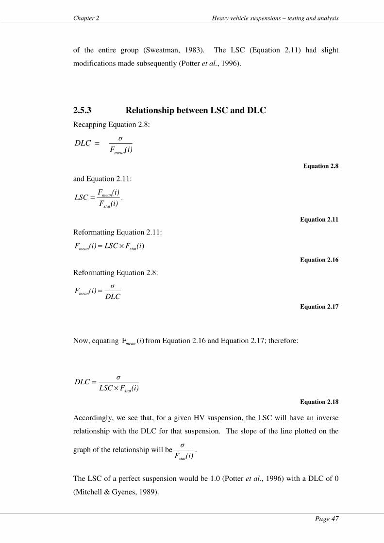
Page 47
Chapter 2 Heavy vehicle suspensions – testing and analysis
of the entire group (Sweatman, 1983). The LSC (Equation 2.11) had slight
modifications made subsequently (Potter et al., 1996).
2.5.3 Relationship between LSC and DLC
Recapping Equation 2.8:
(i)F
σ DLC
mean
=
Equation 2.8
and Equation 2.11:
(i)F
(i)FLSC
stat
mean= .
Equation 2.11
Reformatting Equation 2.11:
)(iFLSC(i)F statmean ×=
Equation 2.16
Reformatting Equation 2.8:
DLC
σ(i)Fmean =
Equation 2.17
Now, equating )(F imean from Equation 2.16 and Equation 2.17; therefore:
(i)FLSC
σDLC
stat×=
Equation 2.18
Accordingly, we see that, for a given HV suspension, the LSC will have an inverse
relationship with the DLC for that suspension. The slope of the line plotted on the
graph of the relationship will be(i)F
σ
stat
.
The LSC of a perfect suspension would be 1.0 (Potter et al., 1996) with a DLC of 0
(Mitchell & Gyenes, 1989).
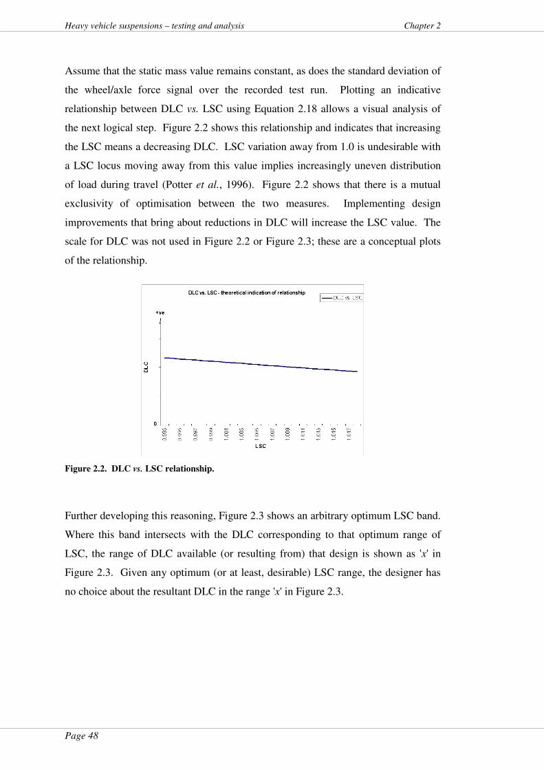
Page 48
Heavy vehicle suspensions – testing and analysis Chapter 2
Assume that the static mass value remains constant, as does the standard deviation of
the wheel/axle force signal over the recorded test run. Plotting an indicative
relationship between DLC vs. LSC using Equation 2.18 allows a visual analysis of
the next logical step. Figure 2.2 shows this relationship and indicates that increasing
the LSC means a decreasing DLC. LSC variation away from 1.0 is undesirable with
a LSC locus moving away from this value implies increasingly uneven distribution
of load during travel (Potter et al., 1996). Figure 2.2 shows that there is a mutual
exclusivity of optimisation between the two measures. Implementing design
improvements that bring about reductions in DLC will increase the LSC value. The
scale for DLC was not used in Figure 2.2 or Figure 2.3; these are a conceptual plots
of the relationship.
Figure 2.2. DLC vs. LSC relationship.
Further developing this reasoning, Figure 2.3 shows an arbitrary optimum LSC band.
Where this band intersects with the DLC corresponding to that optimum range of
LSC, the range of DLC available (or resulting from) that design is shown as 'x' in
Figure 2.3. Given any optimum (or at least, desirable) LSC range, the designer has
no choice about the resultant DLC in the range 'x' in Figure 2.3.
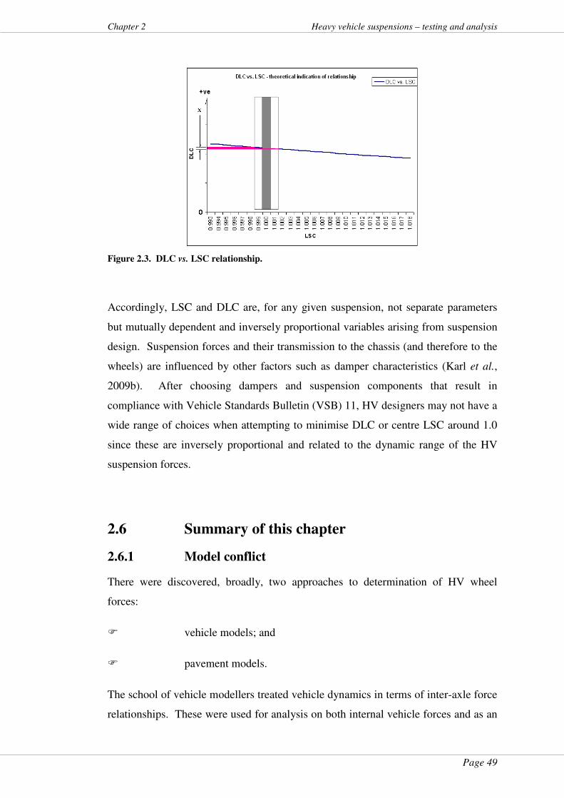
Page 49
Chapter 2 Heavy vehicle suspensions – testing and analysis
Figure 2.3. DLC vs. LSC relationship.
Accordingly, LSC and DLC are, for any given suspension, not separate parameters
but mutually dependent and inversely proportional variables arising from suspension
design. Suspension forces and their transmission to the chassis (and therefore to the
wheels) are influenced by other factors such as damper characteristics (Karl et al.,
2009b). After choosing dampers and suspension components that result in
compliance with Vehicle Standards Bulletin (VSB) 11, HV designers may not have a
wide range of choices when attempting to minimise DLC or centre LSC around 1.0
since these are inversely proportional and related to the dynamic range of the HV
suspension forces.
2.6 Summary of this chapter
2.6.1 Model conflict
There were discovered, broadly, two approaches to determination of HV wheel
forces:
� vehicle models; and
� pavement models.
The school of vehicle modellers treated vehicle dynamics in terms of inter-axle force
relationships. These were used for analysis on both internal vehicle forces and as an
Page 50
Heavy vehicle suspensions – testing and analysis Chapter 2
indication of pavement forces via the wheels. Early work treated load sharing as a
phenomenon involving sequential axles, for example, as opposed to individual
wheels. In contrast, pavement modellers did not concern themselves particularly
about the measurement of pavement forces via axles but applied theoretical and
empirical wheel forces to pavements and modelled the forces where the tyre meets
the road.
2.6.2 Pavement damage models
Pavement damage models may be further separated into differing approaches:
� the “Gaussian” - a random distribution of HV wheel forces on a
road length with all pavement segments subject to a roughly evenly-
distributed probability of road damage; or
� the “spatial” - the characteristics of HV suspensions and travel
speeds incline wheel forces to occur at specific locations on any
length of road and that road damage is therefore concentrated at
those specific points.
As noted in Section 1.4.1, although spatial repetition was acknowledged in the MLR
report, Gaussian distribution of wheel forces was the approach that the National
Road Transport Commission (NRTC) took when considering the introduction of
HML into Australia (National Road Transport Commission, 1993; Pearson & Mass
Limits Review Steering Committee, 1996b).
2.6.3 Spatial repeatability
Adherents to the spatial philosophical school of pavement damage focus on the road
asset, measure wheel forces directly and develop road-damage models that account
for dynamic loads as HVs travel over segments of pavement. This approach
generally requires in-road sensor-based technology to measure actual wheel forces at
the road surface accurately (Cole & Cebon, 1989; Cole, Collop, Potter et al., 1992;
Potter et al., 1996; Potter, Collop, Cole et al., 1994).
Page 51
Chapter 2 Heavy vehicle suspensions – testing and analysis
2.6.4 Spatial repeatability vs. Gaussian distribution
There are some disadvantages with spatial measurement. One is the need for long
lengths of instrumented road, up to 250m (Potter et al., 1997). Another is the
inability to measure conveniently a variety of roads with varying surfaces.
Instrumented vehicles can record data from on-road excitations for longer distances
than an instrumented pavement. On-vehicle measurement ability is more portable,
allowing recording of different road surfaces more conveniently. Further, since road
profiles alter over time, the wheel forces, and therefore road damage, can only be
determined using instrumented pavement methods for the particular set of
circumstances at the time of the testing. Repeatability would require the same length
of pavement to be measured periodically. This is easier with an instrumented vehicle
than an instrumented pavement.
Spatial measures attempt to deal with rutting damage in a different manner from
fatigue damage. Rutting is the result of repeated passes of wheels and is related to
speed and vehicle static mass. Fatigue is a result of many individual dynamic wheel
forces impacting the pavement at the same or similar points along a length of road
(Potter, Cebon, Cole et al., 1995).
Whilst there may be medium-strong spatial correlation of wheel forces for particular
vehicles at particular speeds (Cole et al., 1996), that correlation reduces to moderate-
to-low for the fleet. This is very likely due to different suspension types and
different speeds of operation across the fleet. Accordingly, Eisenmann’s formula
underestimates pavement wear (Gyenes, Mitchell, & Phillips, 1994) and the 95th
percentile formula overestimates pavement wear from dynamic wheel loads
(LeBlanc & Woodrooffe, 1995). That the dominant vehicle types have
approximately Gaussian axle load distributions and therefore may have their wheel
forces characterised by mean and standard deviations has, however, been validated in
more recent work (de Pont, 2004). This assurance was based on DIVINE project
WiM data and incorporated tare as well as loaded data for vehicles representing a
greater majority of HVs on Australian roads.
If spatial measures were valid in predicting pavement failures then peak dynamic
forces would cause those failures (Cole et al., 1996; Collop, Potter, Cebon et al.,
1994). Even if wheel forces were not spatially correlated, the “power law” model for
Page 52
Heavy vehicle suspensions – testing and analysis Chapter 2
wheel force damage would still indicate pavement failure. The difference between
these two models appears to be the number of repetitions before failure rather than
whether to choose average dynamic forces over peak ones.
As pointed out by critics of methods that assume Gaussian distribution of wheel
forces, the “fourth power rule” was developed with dynamic loadings already “built
into” the AASHO experimental data. Different “power law” model exponents have
been derived in the intervening half-Century since the original AASHO work with
military vehicles. The existence of these differing exponents as applied to different
pavement types shows that the “science” of damage models is still not exact.
To exploit spatial repetition as a pure approach, both steady state wheel force load
and dynamic wheel force load need to be separated; pavement damage treated as two
distinct phenomena: rutting and fatigue respectively. In a perfect world, the rutting
and the fatigue damage predictors would be combined after this point in the process
to form a composite damage model. As pointed out by the critics of Gaussian wheel
force models, this is in contradistinction to the “one-size-fits-all” lumped empirical
formula containing both concepts. Nonetheless, and with some awkward logic,
spatial models of pavement damage still nominate the fourth power exponent in their
damage predictions (Collop et al., 1994) for flexible pavements.
2.6.5 Defining road damage from a vehicle-based
framework
Mitchell & Gyenes (1989) noted that one measure alone was not sufficient to
determine the road-damaging potential of a particular suspension and concluded that
a judgement based on:
� LSC;
� DLC;
� low and high frequency vibration forces (body bounce and wheel
hop); and
� peak axle loads

Page 53
Chapter 2 Heavy vehicle suspensions – testing and analysis
would be necessary since the measures developed up to that point described different
suspension parameters, depending on behaviour. Further, it may be valid to question
which parameters should be desirable for “road friendly” suspensions (RFS) as
measured by testing methods other than the European Union method (European
Council, 1996).
de Pont’s work (1999) showed that the values measured for resonant frequencies, etc.
at different loads and speeds do not vary significantly from those derived from the
EU testing if the centre-of-gravity is placed over the particular suspension
(component) under test.
Other research pointed out that determining suspension characteristics measured
from a shaker-bed or reaction frame necessitated either test a single axle with the
body fixed or test the whole vehicle. Testing selected axles did not reflect
suspension nor vehicle performance (Stanzel & Preston-Thomas, 2000). This
inferred that whole-of-vehicle testing is the only valid method but this:
� ignored the reality that prime-movers and trailers are rarely used
continuously as a unit;
� was hard to reconcile against the supposed validity of individual
axle tests; and
� did not seem to encompass de Pont’s work (de Pont, 1999).
2.7 Conclusions of this chapter
2.7.1 Relative views of pavement/wheel load
Pavement forces from a HV may be measured from the viewpoint of the wheels of a
HV or at the pavement. That choice and the assumption of Gaussian force
distribution in the temporal or spatial domains leads to various possibilities for
viewing forces at the HV tyre/pavement interface. The approach of Gaussian
modelling to pavement damage would be valid were HV wheel forces to be
distributed randomly along a length of road. This relies on measurement of wheel
force histories (statistical analysis) and development of road-damage models based
Page 54
Heavy vehicle suspensions – testing and analysis Chapter 2
on (say) the “fourth power rule”. Pavement design life is then based on repetitive
loadings arising from repeated passes of a theoretical heavy vehicle axle. That
thinking may be applied to either vehicle-based or pavement-based measurements.
The former approach, where pavement effects are assumed from measured wheel
forces, is more common since HVs are more easily instrumented than pavements.
Alternative approaches in the pavement modelling domain measure wheel forces
directly and develop road-damage models that account for dynamic loads as HVs
travel over segments of pavement. This generally requires in-road sensors to
measure wheel forces at the road surface (Cole & Cebon, 1989; Cole et al., 1992;
Potter et al., 1996; Potter et al., 1994).
2.7.2 Spatial repeatability vs. Gaussian distribution
The spatial school, backed by not inconsiderable empirical data, rejects the thinking
of the Gaussians and contends that spatial repetition will cause failure of the
pavement from localised peak dynamic forces damaging the pavement at recurrent
points along a length of road. It rejects the use of averaged dynamic forces as a
predictor of pavement damage (Potter et al., 1994). This philosophy then proposes
that network utility is reduced by denying service on the road where such localised
pavement failures occur (Cebon, 1987, 1993, 1999). This may be balanced against a
pragmatic view that such service denial is short-term; potholes are patched with
subsequent resumption of access, whilst conceding that patches increase future
failure point probability.
2.7.3 Vehicle-centric measurement of metrics
In striving to improve the LSC or DLC suspension metrics, the vehicle designer may
not have much choice as these are mutually dependent variables and inversely
proportional to each other. Improving one degrades the other.
There is a broad range of suspension metrics available to the vehicle researcher or
designer. Some of these are more easily derived than others. The mechanisms for
Page 55
Chapter 2 Heavy vehicle suspensions – testing and analysis
creating the necessary vehicle dynamics to measure the metrics vary from the simple
to the complex. Computational requirements for deriving the various metrics vary
likewise.
Early work (Eisenmann, 1975; Sweatman, 1983) postulated certain approaches,
particularly assuming Gaussian distribution of wheel forces. Later development,
leveraging off spatial repetition, adopted a reductionist approach and concentrated
more on peak wheel forces as an indicator of pavement damage (Fletcher et al.,
2002; Woodrooffe & LeBlanc, 1987). This latter metric much more easily measured,
either from the vehicle or the pavement.
2.7.4 Pavement models
Whether wheel forces are measured at the pavement or the vehicle, whether they are
aligned spatially or which metrics are valid; pavement models, particularly in
Australia, ascribe pavement life design to quasi-static HV axle load repetitions with a
“power law” damage exponent. These models are empirically derived from data that
contains both static and dynamic wheel forces. Section 2.4.2 expanded on these
damage exponents.
Pavement damage models have an entrained “power law” damage exponent to
account for empirical data drawn from different countries, differing materials and
different HV configurations (Pidwerbesky, 1989). Damage exponents varying from
1 to 8 for flexible pavements (de Pont & Steven, 1999; Pidwerbesky, 1989) and up to
12 for concrete pavements (Austroads, 1992; Vuong, 2009) are used. dePont &
Steven (1999) showed quasi-static loadings caused rutting but not fatigue, with
damage exponents tending toward 1.0.
The damage exponent order of magnitude varied in the literature from x1 to x12. This
range is greater than the order of magnitude variation in the exponents allocated to
human scale (100 m) vs. Earth diameter (107 m). From the original derivation of the
repetitive axle loading and subsequent evolution of pavement damage models, it
appears that the variation in order-of-magnitude of damage exponents has been a
result of explaining subsequent pavement damage empirical data in various ways.

Page 56
Heavy vehicle suspensions – testing and analysis Chapter 2
Notwithstanding, it is difficult to reconcile that variations in HVs, materials and
country of construction would account for damage outcomes greater than the
proportion of a human to the size of the Earth.
In summary, the Gaussian vs. spatial and HV instruments vs. in-road sensor debates
will largely be academic until standard axle repetition (SAR) or equivalent standard
axle (ESA) measures incorporate scientifically-determined dynamic wheel force
measures. Whilst the fourth power rule and ESAs have been questioned, they remain
in pavement engineering lore as the basis of measures to determine asset damage.
2.8 Chapter close
The research framework, problem statements and objectives for this thesis were
outlined in Chapter 1. However, without tools to execute the work (or parameters to
measure, analyse and report) the research programme would be for nothing.
Accordingly, this chapter introduced the philosophy, derivation and range of
available HV suspension metrics and their measurement. The background described
in this chapter informed the methodology and rationale embedded in the testing
procedures, particularly digital sampling theory (Section 2.3.3), used to gather the
data for the project Heavy vehicle suspensions – testing and analysis. These
procedures are detailed in Chapter 3 following.
Chapter 4 details the development heavy vehicle (HV) suspension models for the
thesis. This process would be less intelligible without the introduction to damping
ratio and damped natural frequency in Sections 2.3.1 and 2.3.2.
Analysis of the data testing from the testing outlined in Chapter 3 will be presented
later in this thesis in Chapters 5 to 10. These chapters will make extensive use of HV
suspension metrics detailed in Chapter 2.
Chapter 8, whilst mostly concerned with on-board mass (OBM) measurement
systems for HVs, will require a working knowledge of the fundamental
characteristics of a HV suspension as provided in Chapter 2, particularly digital
sampling theory (Section 2.3.3).
Page 57
Chapter 2 Heavy vehicle suspensions – testing and analysis
Links where this chapter informs other chapters of this thesis are shown in Figure
1.4.
“If you are not measuring it, you are not managing it.” - W. Ed Deming.
Page 58
Heavy vehicle suspensions – testing and analysis Chapter 3
3 Test methodology arising from problem
identification
3.1 About this chapter
This chapter describes the methodology used to gather the data for the project: Heavy
vehicle suspensions – testing and analysis. This includes the rationale for choices
made when designing the tests.
3.1.1 Rationale for sampling frequency – general statement
regarding Sections 3.2 and 3.3
Data for use to meet Objectives 1 and 2 (the three heavy vehicles in Section 3.2) and
Objective 3 (the roller bed testing in section 3.3) were recorded using an advanced
version of a CHEK-WAY® HV telemetry system. The telemetry system sampling
rate was 1 kHz giving a sample period of 1.0 ms. The natural frequency of a typical
heavy vehicle axle (axle-hop) is 10 to 15 Hz; a natural periodicity in the range 100 to
66.7 ms (Cebon, 1999). The sprung mass damped natural frequency or body bounce
is usually in the range 1 to 4 Hz; a natural periodicity in the range 1000 to 250 ms
and therefore of a relatively lower frequency range (i.e. greater periodicity values)
than axle-hop (de Pont, 1999).
The Nyquist sampling criterion (Shannon’s theorem) defines the minimum required
sampling frequency for any dynamic data. For accurate recreation of dynamic data
from sampled data without loss of information, Shannon’s theorem specifies that
measured dynamic data be sampled at a frequency at least twice that of the highest
data frequency of interest (Houpis & Lamont, 1985). The supporting theoretical
background for this has been covered in Section 2.3.3. When using time-based
recording, measuring and reconstruction of signals with higher frequencies than (say)
body bounce, such as axle-hop, necessitates higher sampling rates than would be
used for body bounce data. The maximum frequency in the data for the testing
described in Section 3.2 and Section 3.3 was 15 Hz (axle-hop); the corresponding
minimum necessary sampling frequency was therefore 30 Hz. The CHEK-WAY®
HV telemetry system sampling frequency of 1 kHz was well above the minimum
requirement of 30 Hz; the requirement for the Nyquist sampling criterion (Shannon’s
Page 59
Chapter 3 Heavy vehicle suspensions – testing and analysis
theorem) was therefore met for the testing.
3.2 HV suspension testing - Objective 2 and part of
Objective 3
A test programme used three instrumented heavy vehicles (HVs) to gather data used
for determining whether larger longitudinal air lines alter wheel or chassis forces
(Objective 2) in addition to informing part of the in-service suspension testing
(Objective 3) portion of this project.
3.2.1 General description
To provide data for Objective 2 and partially for Objective 3, the wheel forces and
chassis forces on three test HVs were measured. The test HVs and their axle group
configurations were as follows:
� School bus: one front steer axle, one rear (drive) axle;
� Interstate coach: one front steer axle, one rear drive axle, one rear
tag axle. The tag and drive axle comprised the rear axle group.
Axle spacing between the tag axle and the drive axle was 1.4 m; and
� Articulated HV: prime mover (not tested) and trailer tri-axle group
with axle spacing of 1.4 m.
These are shown from Figure 3.1 to Figure 3.4. The semi-trailer was towed by a
prime mover that was not tested in this programme.
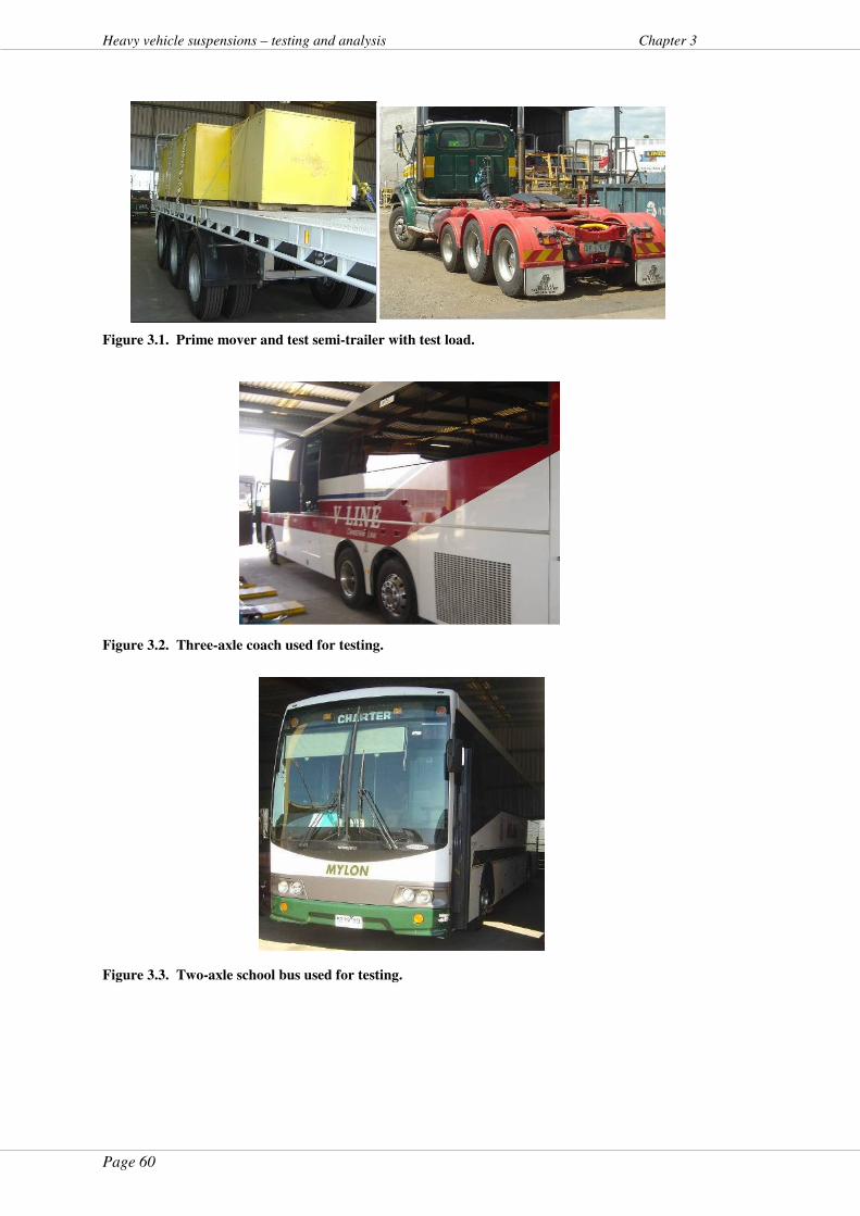
Page 60
Heavy vehicle suspensions – testing and analysis Chapter 3
Figure 3.1. Prime mover and test semi-trailer with test load.
Figure 3.2. Three-axle coach used for testing.
Figure 3.3. Two-axle school bus used for testing.
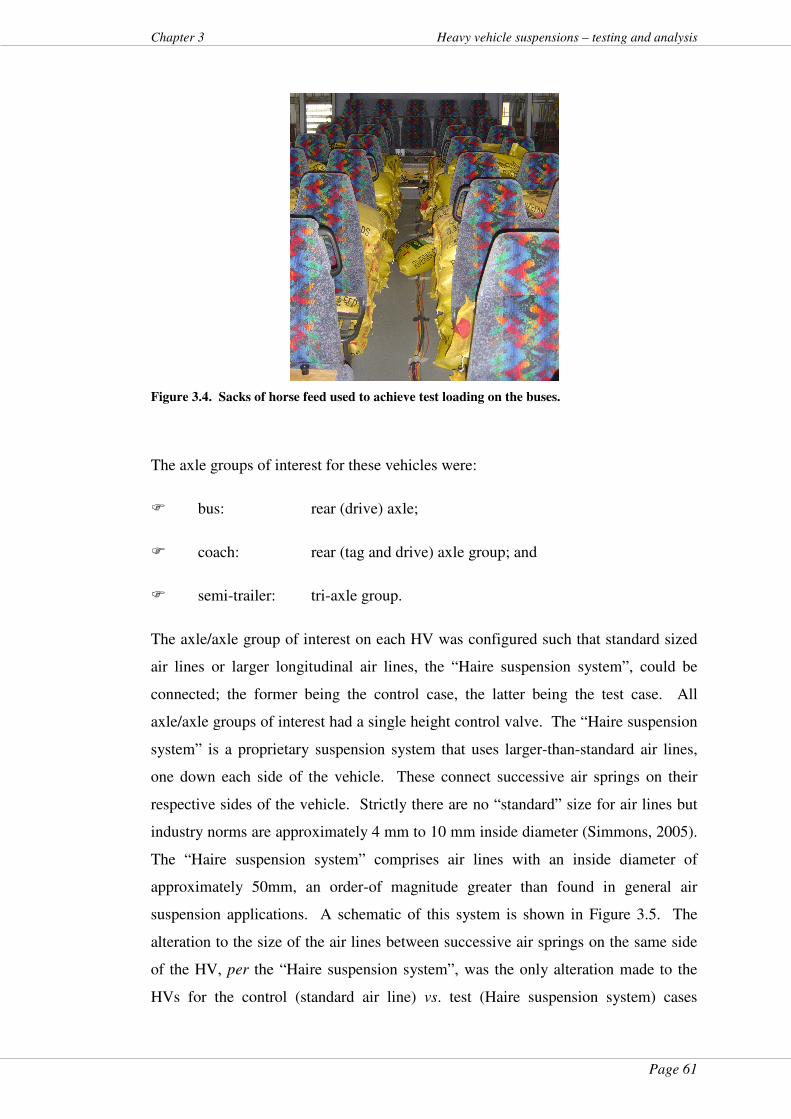
Page 61
Chapter 3 Heavy vehicle suspensions – testing and analysis
Figure 3.4. Sacks of horse feed used to achieve test loading on the buses.
The axle groups of interest for these vehicles were:
� bus: rear (drive) axle;
� coach: rear (tag and drive) axle group; and
� semi-trailer: tri-axle group.
The axle/axle group of interest on each HV was configured such that standard sized
air lines or larger longitudinal air lines, the “Haire suspension system”, could be
connected; the former being the control case, the latter being the test case. All
axle/axle groups of interest had a single height control valve. The “Haire suspension
system” is a proprietary suspension system that uses larger-than-standard air lines,
one down each side of the vehicle. These connect successive air springs on their
respective sides of the vehicle. Strictly there are no “standard” size for air lines but
industry norms are approximately 4 mm to 10 mm inside diameter (Simmons, 2005).
The “Haire suspension system” comprises air lines with an inside diameter of
approximately 50mm, an order-of magnitude greater than found in general air
suspension applications. A schematic of this system is shown in Figure 3.5. The
alteration to the size of the air lines between successive air springs on the same side
of the HV, per the “Haire suspension system”, was the only alteration made to the
HVs for the control (standard air line) vs. test (Haire suspension system) cases
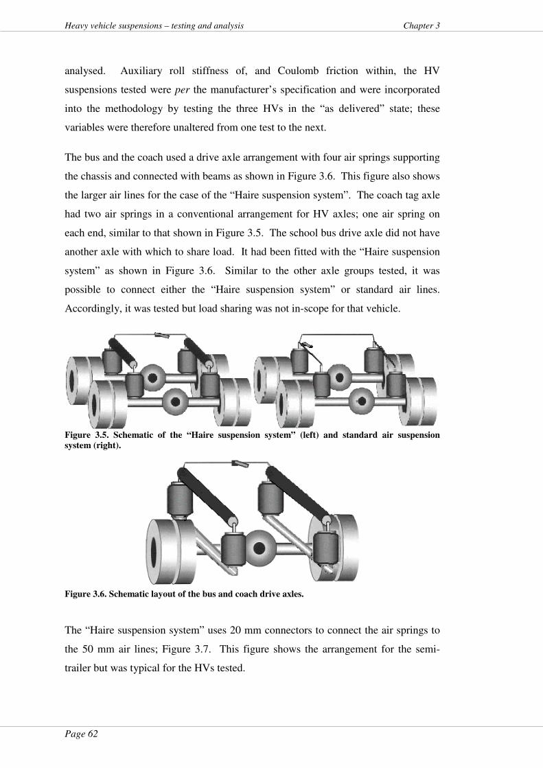
Page 62
Heavy vehicle suspensions – testing and analysis Chapter 3
analysed. Auxiliary roll stiffness of, and Coulomb friction within, the HV
suspensions tested were per the manufacturer’s specification and were incorporated
into the methodology by testing the three HVs in the “as delivered” state; these
variables were therefore unaltered from one test to the next.
The bus and the coach used a drive axle arrangement with four air springs supporting
the chassis and connected with beams as shown in Figure 3.6. This figure also shows
the larger air lines for the case of the “Haire suspension system”. The coach tag axle
had two air springs in a conventional arrangement for HV axles; one air spring on
each end, similar to that shown in Figure 3.5. The school bus drive axle did not have
another axle with which to share load. It had been fitted with the “Haire suspension
system” as shown in Figure 3.6. Similar to the other axle groups tested, it was
possible to connect either the “Haire suspension system” or standard air lines.
Accordingly, it was tested but load sharing was not in-scope for that vehicle.
Figure 3.5. Schematic of the “Haire suspension system” (left) and standard air suspension
system (right).
Figure 3.6. Schematic layout of the bus and coach drive axles.
The “Haire suspension system” uses 20 mm connectors to connect the air springs to
the 50 mm air lines; Figure 3.7. This figure shows the arrangement for the semi-
trailer but was typical for the HVs tested.
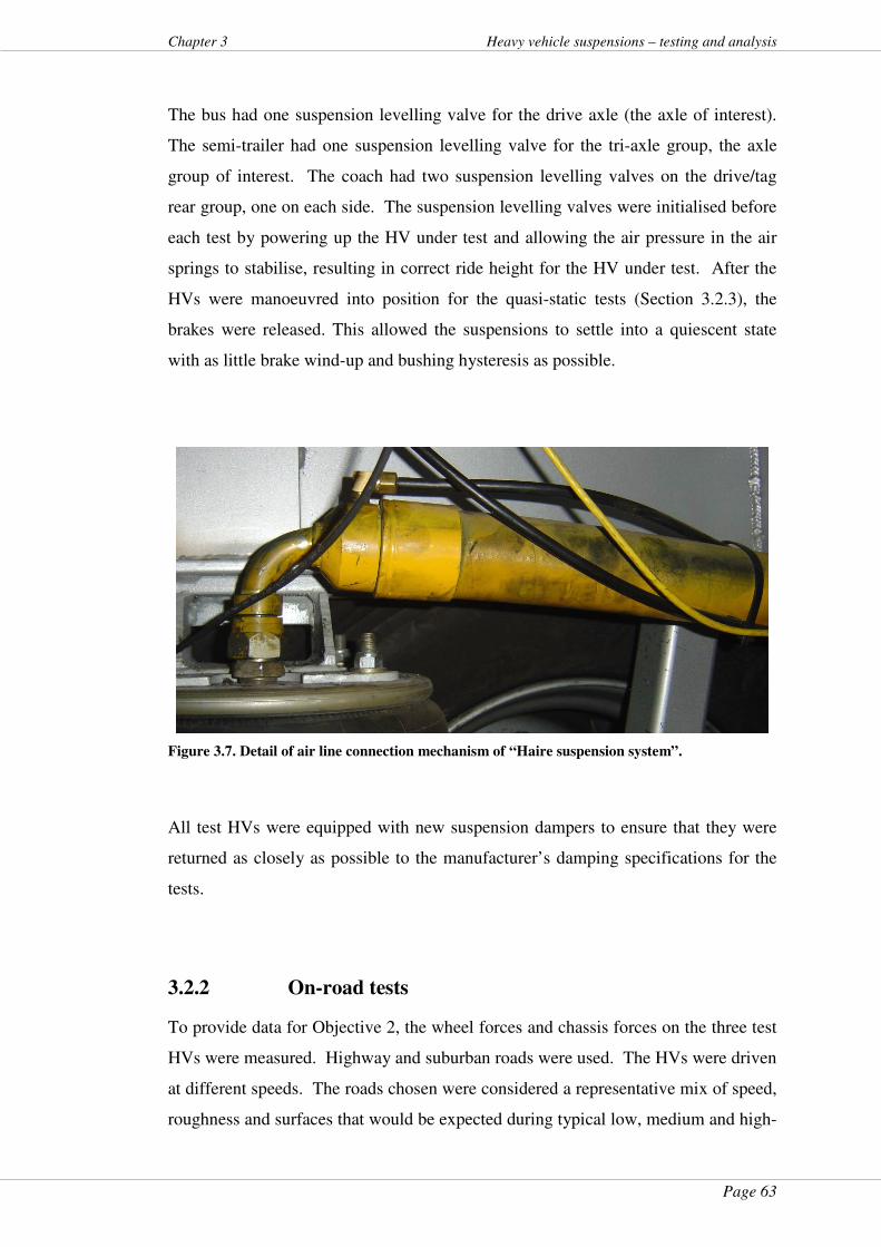
Page 63
Chapter 3 Heavy vehicle suspensions – testing and analysis
The bus had one suspension levelling valve for the drive axle (the axle of interest).
The semi-trailer had one suspension levelling valve for the tri-axle group, the axle
group of interest. The coach had two suspension levelling valves on the drive/tag
rear group, one on each side. The suspension levelling valves were initialised before
each test by powering up the HV under test and allowing the air pressure in the air
springs to stabilise, resulting in correct ride height for the HV under test. After the
HVs were manoeuvred into position for the quasi-static tests (Section 3.2.3), the
brakes were released. This allowed the suspensions to settle into a quiescent state
with as little brake wind-up and bushing hysteresis as possible.
Figure 3.7. Detail of air line connection mechanism of “Haire suspension system”.
All test HVs were equipped with new suspension dampers to ensure that they were
returned as closely as possible to the manufacturer’s damping specifications for the
tests.
3.2.2 On-road tests
To provide data for Objective 2, the wheel forces and chassis forces on the three test
HVs were measured. Highway and suburban roads were used. The HVs were driven
at different speeds. The roads chosen were considered a representative mix of speed,
roughness and surfaces that would be expected during typical low, medium and high-

Page 64
Heavy vehicle suspensions – testing and analysis Chapter 3
speed HV operation. The road sections were in the Brisbane area; locations and
speeds were as shown in Table 3.1.
The test HVs were tested both at tare and loaded, the loaded case being as close to
the maximum general access mass for the group under test. Scrap steel in bins was
used to load the semi-trailer (Figure 3.1 and Figure 3.11); sacks of horse feed were
used to load the buses (Figure 3.4).
The test HVs were instrumented to measure axle-to-chassis forces and wheel forces.
The dynamic signals from the on-board instrumentation were recorded for 10 s at 1.0
kHz. This resulted in test data in the form of 10,000 data points over a 10 s time-
series signal from the transducers at each axle-end of interest on each test HV at the
various test speeds.
The same section of road was not used for each speed during these tests. For reasons
of logistics, safety and consideration of other road users, the general speed limit on
each road section was used as the test speed.
Table 3.1. Test speeds, locations and details for the three HVs.
Location Description Speed
(km/h)
Sherwood Rd, Rocklea
Westbound after the traffic signals at the Rocklea markets
40 and 60
Fairfield Rd, Rocklea and
Fairfield
Northbound after the roundabout at Venner Rd
60
Fairfield Rd, Rocklea and
Fairfield Northbound after the Hi-Trans depot 60 and 70
Ipswich Mwy Westbound under the Oxley
Rd/Blunder Rd overpass 80 and 90
Ipswich Mwy N/Eastbound after the Progress Rd on-
ramp 80 and 90
Nonetheless, different roads with different roughness at different speeds have been
used previously and was not an unusual approach for this type of testing
(Woodrooffe, LeBlanc, & LePiane, 1986). Another consideration was that a variety
of surface roughness was not available over one section of road for a variety of
speeds within the 10 s recording window of the telemetry system. The testing
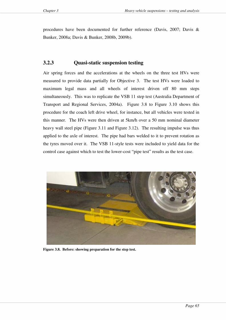
Page 65
Chapter 3 Heavy vehicle suspensions – testing and analysis
procedures have been documented for further reference (Davis, 2007; Davis &
Bunker, 2008a; Davis & Bunker, 2008b, 2009b).
3.2.3 Quasi-static suspension testing
Air spring forces and the accelerations at the wheels on the three test HVs were
measured to provide data partially for Objective 3. The test HVs were loaded to
maximum legal mass and all wheels of interest driven off 80 mm steps
simultaneously. This was to replicate the VSB 11 step test (Australia Department of
Transport and Regional Services, 2004a). Figure 3.8 to Figure 3.10 shows this
procedure for the coach left drive wheel, for instance, but all vehicles were tested in
this manner. The HVs were then driven at 5km/h over a 50 mm nominal diameter
heavy wall steel pipe (Figure 3.11 and Figure 3.12). The resulting impulse was thus
applied to the axle of interest. The pipe had bars welded to it to prevent rotation as
the tyres moved over it. The VSB 11-style tests were included to yield data for the
control case against which to test the lower-cost “pipe test” results as the test case.
Figure 3.8. Before: showing preparation for the step test.
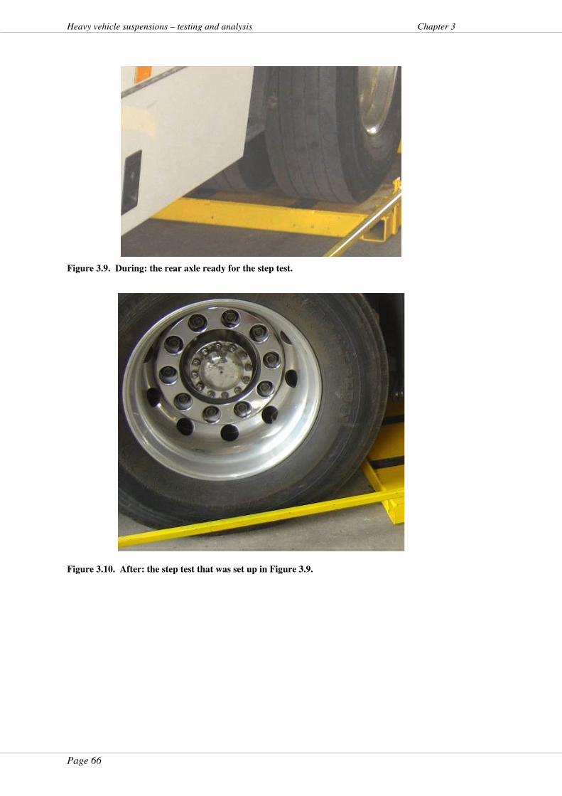
Page 66
Heavy vehicle suspensions – testing and analysis Chapter 3
Figure 3.9. During: the rear axle ready for the step test.
Figure 3.10. After: the step test that was set up in Figure 3.9.
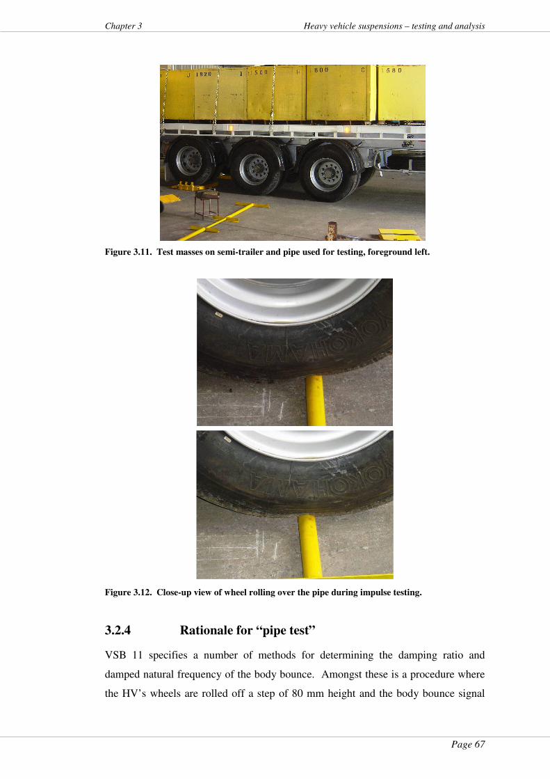
Page 67
Chapter 3 Heavy vehicle suspensions – testing and analysis
Figure 3.11. Test masses on semi-trailer and pipe used for testing, foreground left.
Figure 3.12. Close-up view of wheel rolling over the pipe during impulse testing.
3.2.4 Rationale for “pipe test”
VSB 11 specifies a number of methods for determining the damping ratio and
damped natural frequency of the body bounce. Amongst these is a procedure where
the HV’s wheels are rolled off a step of 80 mm height and the body bounce signal
Page 68
Heavy vehicle suspensions – testing and analysis Chapter 3
analysed. System theory has it that a resonant system may be characterised by
analysis of the system output after an impulse input (Chesmond, 1982; Considine,
1985; Doebelin, 1980). Inputs into systems are also known as “forcing functions”.
The background to this portion of systems theory is that a perfect impulse of
infinitely short period will contain all frequencies. Infinitely short impulses have,
theoretically, infinite power. The characteristic frequencies of the system will be the
ones transmitted to the output after such an input and thus available for analysis.
Pragmatically, no impulse is of infinitely short duration, nor of infinite power.
However, the application of this theory works well in practice, provided the forcing
function is as short as possible and of a period less than 0.35 the damped natural
period (Doebelin, 1980). That work also showed that the shape of the forcing
function was not relevant provided that it was short enough (i.e. of a shorter duration
than 0.35 of the natural period of the system being characterised). The 80 mm step,
in terms of system theory behind that particular VSB 11 method, was the impulse
imparted to the HV suspensions to excite them, as systems, so that their outputs,
being the axle-to-body displacements, could each be analysed for damped natural
frequency and damping ratio. To inform Objective 3 (in-service suspension testing)
partially, the “pipe test” was proposed as an alternative, lower cost, forcing function
to the step test.
3.2.5 Rationale for instrumentation to measure dynamic
wheel forces
To inform Objective 2 (alterations to dynamic load sharing from larger longitudinal
air lines) and partially Objective 3 (in-service suspension testing) wheel forces and
hub acceleration data were required. A combination of accelerometers and strain
gauges was necessary to measure wheel forces.
Strain gauges were mounted on the sides of the axles of interest. This positioned
them across the neutral axis of the axle to be measured. Mounting was as close as
possible to the hub and used cyanoacrylate glue after surface polishing. Figure 3.13
shows the arrangement for the semi-trailer, for example, but this was typical for all
the test vehicles. Waterproofing foil was installed over the strain gauges.
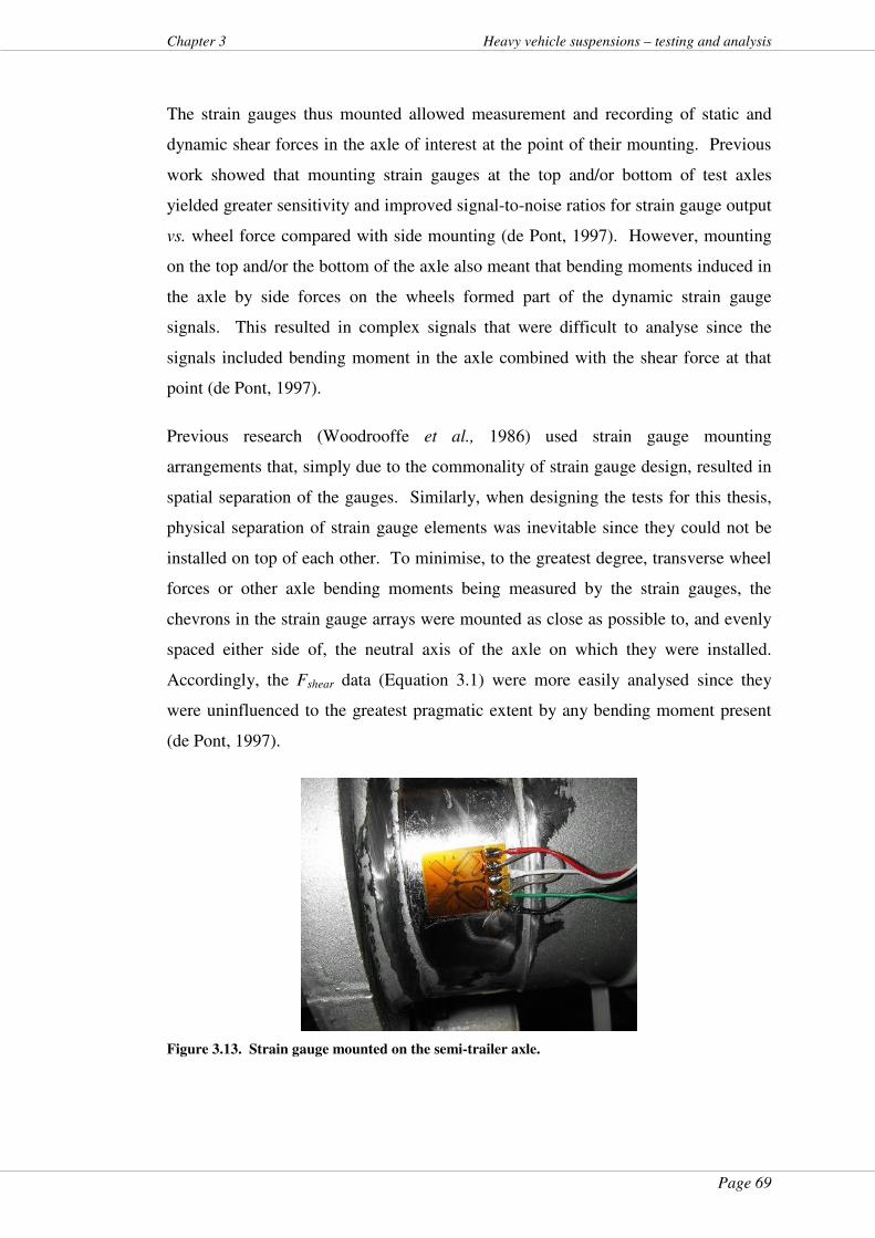
Page 69
Chapter 3 Heavy vehicle suspensions – testing and analysis
The strain gauges thus mounted allowed measurement and recording of static and
dynamic shear forces in the axle of interest at the point of their mounting. Previous
work showed that mounting strain gauges at the top and/or bottom of test axles
yielded greater sensitivity and improved signal-to-noise ratios for strain gauge output
vs. wheel force compared with side mounting (de Pont, 1997). However, mounting
on the top and/or the bottom of the axle also meant that bending moments induced in
the axle by side forces on the wheels formed part of the dynamic strain gauge
signals. This resulted in complex signals that were difficult to analyse since the
signals included bending moment in the axle combined with the shear force at that
point (de Pont, 1997).
Previous research (Woodrooffe et al., 1986) used strain gauge mounting
arrangements that, simply due to the commonality of strain gauge design, resulted in
spatial separation of the gauges. Similarly, when designing the tests for this thesis,
physical separation of strain gauge elements was inevitable since they could not be
installed on top of each other. To minimise, to the greatest degree, transverse wheel
forces or other axle bending moments being measured by the strain gauges, the
chevrons in the strain gauge arrays were mounted as close as possible to, and evenly
spaced either side of, the neutral axis of the axle on which they were installed.
Accordingly, the Fshear data (Equation 3.1) were more easily analysed since they
were uninfluenced to the greatest pragmatic extent by any bending moment present
(de Pont, 1997).
Figure 3.13. Strain gauge mounted on the semi-trailer axle.
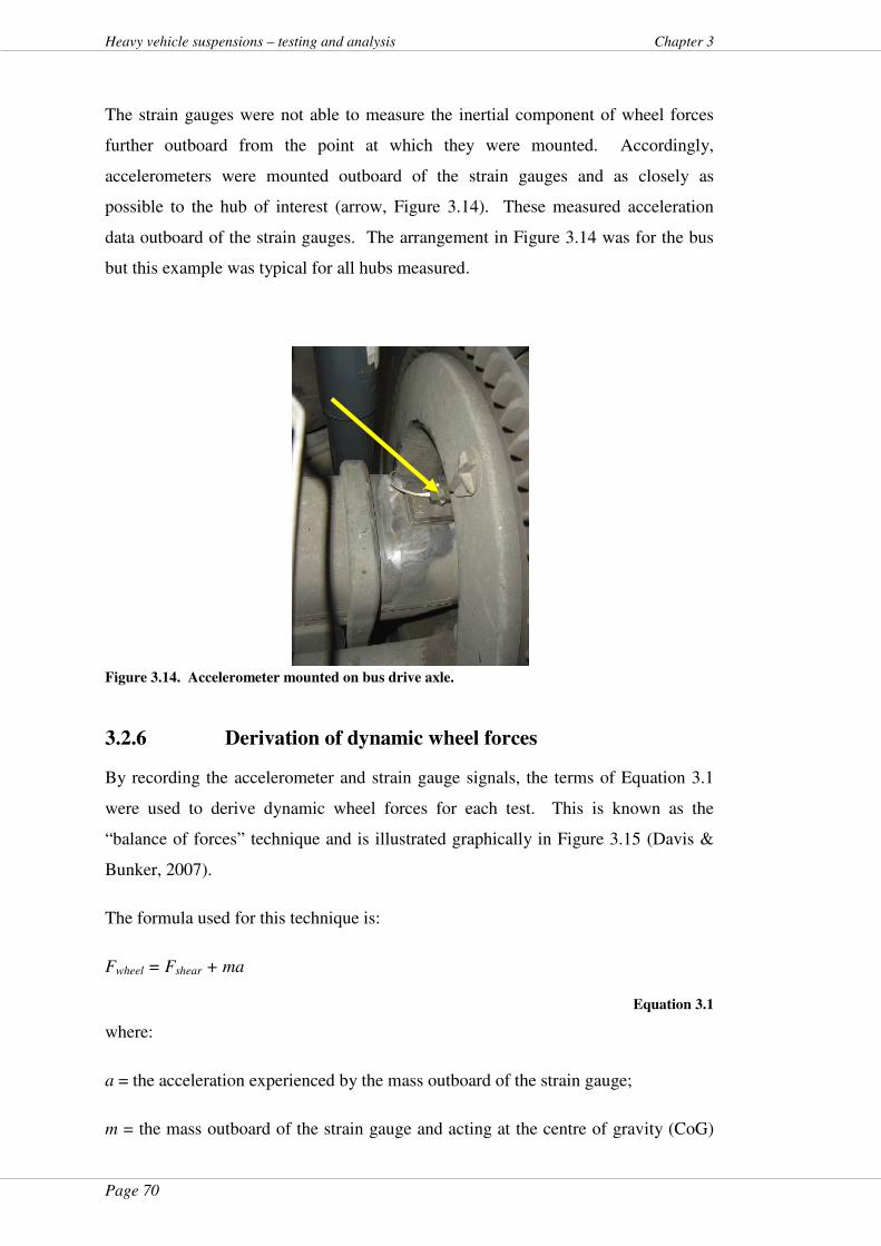
Page 70
Heavy vehicle suspensions – testing and analysis Chapter 3
The strain gauges were not able to measure the inertial component of wheel forces
further outboard from the point at which they were mounted. Accordingly,
accelerometers were mounted outboard of the strain gauges and as closely as
possible to the hub of interest (arrow, Figure 3.14). These measured acceleration
data outboard of the strain gauges. The arrangement in Figure 3.14 was for the bus
but this example was typical for all hubs measured.
Figure 3.14. Accelerometer mounted on bus drive axle.
3.2.6 Derivation of dynamic wheel forces
By recording the accelerometer and strain gauge signals, the terms of Equation 3.1
were used to derive dynamic wheel forces for each test. This is known as the
“balance of forces” technique and is illustrated graphically in Figure 3.15 (Davis &
Bunker, 2007).
The formula used for this technique is:
Fwheel = Fshear + ma
Equation 3.1
where:
a = the acceleration experienced by the mass outboard of the strain gauge;
m = the mass outboard of the strain gauge and acting at the centre of gravity (CoG)
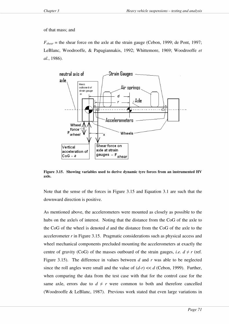
Page 71
Chapter 3 Heavy vehicle suspensions – testing and analysis
of that mass; and
Fshear = the shear force on the axle at the strain gauge (Cebon, 1999; de Pont, 1997;
LeBlanc, Woodrooffe, & Papagiannakis, 1992; Whittemore, 1969; Woodrooffe et
al., 1986).
Figure 3.15. Showing variables used to derive dynamic tyre forces from an instrumented HV
axle.
Note that the sense of the forces in Figure 3.15 and Equation 3.1 are such that the
downward direction is positive.
As mentioned above, the accelerometers were mounted as closely as possible to the
hubs on the axle/s of interest. Noting that the distance from the CoG of the axle to
the CoG of the wheel is denoted d and the distance from the CoG of the axle to the
accelerometer r in Figure 3.15. Pragmatic considerations such as physical access and
wheel mechanical components precluded mounting the accelerometers at exactly the
centre of gravity (CoG) of the masses outboard of the strain gauges, i.e. d ≠ r (ref.
Figure 3.15). The difference in values between d and r was able to be neglected
since the roll angles were small and the value of (d-r) << d (Cebon, 1999). Further,
when comparing the data from the test case with that for the control case for the
same axle, errors due to d ≠ r were common to both and therefore cancelled
(Woodrooffe & LeBlanc, 1987). Previous work stated that even large variations in

Page 72
Heavy vehicle suspensions – testing and analysis Chapter 3
the forces outboard of the strain gauges do not contribute greatly to the overall
variation in measured wheel forces (de Pont, 1997).
The values of m for the three test HVs were found from manufacturer’s data
(Giacomini, 2007; Mack-Volvo, 2007a), calculation of trailer axle tube mass using
steel density and by direct measurement. The direct measurement technique was
used for the bus and the coach and involved cutting through damaged axle housings
at the corresponding strain gauge mounting point. The axle remnants outboard of the
respective strain gauge mounting points were then weighed (Appendix 1).
Further details of the rationale for the instrumentation, calibration and the
methodology used in the derivation of the wheel forces have been documented in
Appendix 1 and previous publications (Davis, 2007; Davis & Bunker, 2008a; Davis
& Bunker, 2008b, 2009b).
3.2.7 Rationale for instrumentation – indicative pavement
roughness
To inform Objective 2 (alterations to dynamic load sharing from larger longitudinal
air lines) roughness values of the pavements encountered were derived. The
accelerometer signals from the on-road testing were used to derive indicative
roughness values. This was designated the “novel roughness” value to distinguish it
from the standard definition of roughness used by pavement engineers. The usual
definition of road roughness is an international standard measure termed the
international roughness index (IRI). It is found by calibrated vehicles performing
test runs. The data from such a run is a roughness measure of the tested pavement in
mm/m or m/km. This is indicative of the amount of vertical movement of the
calibrated vehicle relative to the horizontal distance travelled along the road during
the test run. This measure may also be visualised as an upward slope that the vehicle
negotiates as it travels. The steepness of the slope is proportional to the roughness of
the road. This measure is now standardised for world-wide use (Sayers, Gillespie, &
Hagan, 1987; Sayers, Gillespie, & Paterson, 1986).
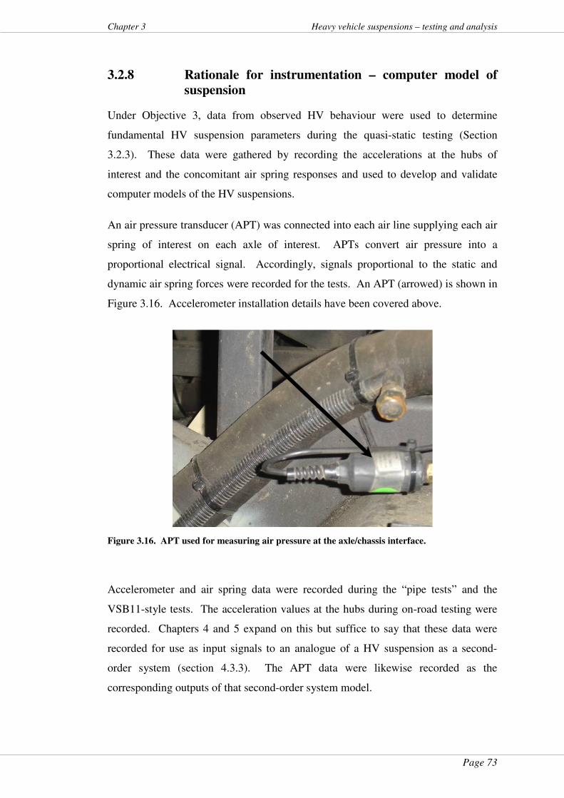
Page 73
Chapter 3 Heavy vehicle suspensions – testing and analysis
3.2.8 Rationale for instrumentation – computer model of
suspension
Under Objective 3, data from observed HV behaviour were used to determine
fundamental HV suspension parameters during the quasi-static testing (Section
3.2.3). These data were gathered by recording the accelerations at the hubs of
interest and the concomitant air spring responses and used to develop and validate
computer models of the HV suspensions.
An air pressure transducer (APT) was connected into each air line supplying each air
spring of interest on each axle of interest. APTs convert air pressure into a
proportional electrical signal. Accordingly, signals proportional to the static and
dynamic air spring forces were recorded for the tests. An APT (arrowed) is shown in
Figure 3.16. Accelerometer installation details have been covered above.
Figure 3.16. APT used for measuring air pressure at the axle/chassis interface.
Accelerometer and air spring data were recorded during the “pipe tests” and the
VSB11-style tests. The acceleration values at the hubs during on-road testing were
recorded. Chapters 4 and 5 expand on this but suffice to say that these data were
recorded for use as input signals to an analogue of a HV suspension as a second-
order system (section 4.3.3). The APT data were likewise recorded as the
corresponding outputs of that second-order system model.
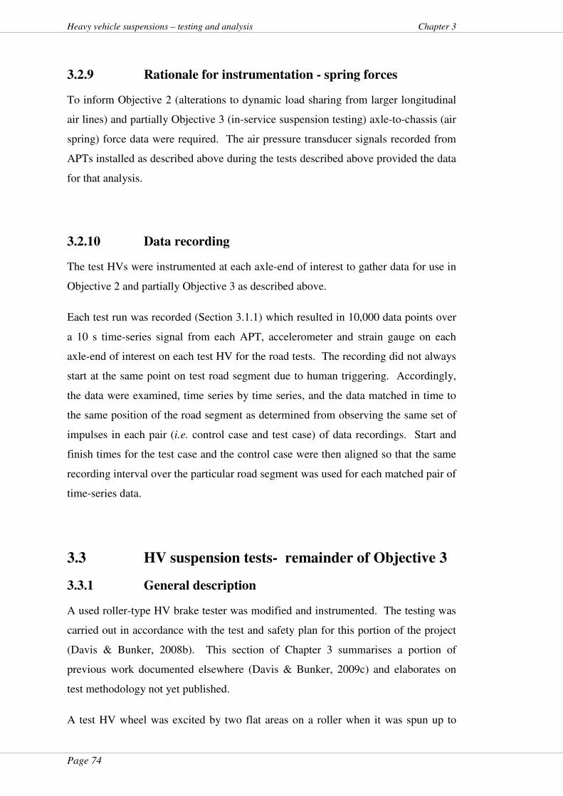
Page 74
Heavy vehicle suspensions – testing and analysis Chapter 3
3.2.9 Rationale for instrumentation - spring forces
To inform Objective 2 (alterations to dynamic load sharing from larger longitudinal
air lines) and partially Objective 3 (in-service suspension testing) axle-to-chassis (air
spring) force data were required. The air pressure transducer signals recorded from
APTs installed as described above during the tests described above provided the data
for that analysis.
3.2.10 Data recording
The test HVs were instrumented at each axle-end of interest to gather data for use in
Objective 2 and partially Objective 3 as described above.
Each test run was recorded (Section 3.1.1) which resulted in 10,000 data points over
a 10 s time-series signal from each APT, accelerometer and strain gauge on each
axle-end of interest on each test HV for the road tests. The recording did not always
start at the same point on test road segment due to human triggering. Accordingly,
the data were examined, time series by time series, and the data matched in time to
the same position of the road segment as determined from observing the same set of
impulses in each pair (i.e. control case and test case) of data recordings. Start and
finish times for the test case and the control case were then aligned so that the same
recording interval over the particular road segment was used for each matched pair of
time-series data.
3.3 HV suspension tests- remainder of Objective 3
3.3.1 General description
A used roller-type HV brake tester was modified and instrumented. The testing was
carried out in accordance with the test and safety plan for this portion of the project
(Davis & Bunker, 2008b). This section of Chapter 3 summarises a portion of
previous work documented elsewhere (Davis & Bunker, 2009c) and elaborates on
test methodology not yet published.
A test HV wheel was excited by two flat areas on a roller when it was spun up to
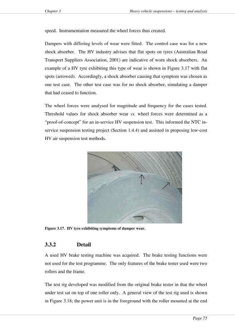
Page 75
Chapter 3 Heavy vehicle suspensions – testing and analysis
speed. Instrumentation measured the wheel forces thus created.
Dampers with differing levels of wear were fitted. The control case was for a new
shock absorber. The HV industry advises that flat spots on tyres (Australian Road
Transport Suppliers Association, 2001) are indicative of worn shock absorbers. An
example of a HV tyre exhibiting this type of wear is shown in Figure 3.17 with flat
spots (arrowed). Accordingly, a shock absorber causing that symptom was chosen as
one test case. The other test case was for no shock absorber, simulating a damper
that had ceased to function.
The wheel forces were analysed for magnitude and frequency for the cases tested.
Threshold values for shock absorber wear vs. wheel forces were determined as a
“proof-of-concept” for an in-service HV suspension test. This informed the NTC in-
service suspension testing project (Section 1.4.4) and assisted in proposing low-cost
HV air suspension test methods.
Figure 3.17. HV tyre exhibiting symptoms of damper wear.
3.3.2 Detail
A used HV brake testing machine was acquired. The brake testing functions were
not used for the test programme. The only features of the brake tester used were two
rollers and the frame.
The test rig developed was modified from the original brake tester in that the wheel
under test sat on top of one roller only. A general view of the test rig used is shown
in Figure 3.18; the power unit is in the foreground with the roller mounted at the end
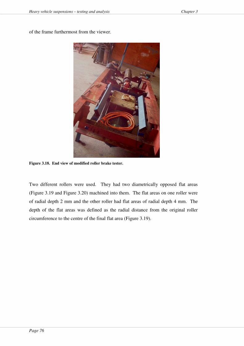
Page 76
Heavy vehicle suspensions – testing and analysis Chapter 3
of the frame furthermost from the viewer.
Figure 3.18. End view of modified roller brake tester.
Two different rollers were used. They had two diametrically opposed flat areas
(Figure 3.19 and Figure 3.20) machined into them. The flat areas on one roller were
of radial depth 2 mm and the other roller had flat areas of radial depth 4 mm. The
depth of the flat areas was defined as the radial distance from the original roller
circumference to the centre of the final flat area (Figure 3.19).
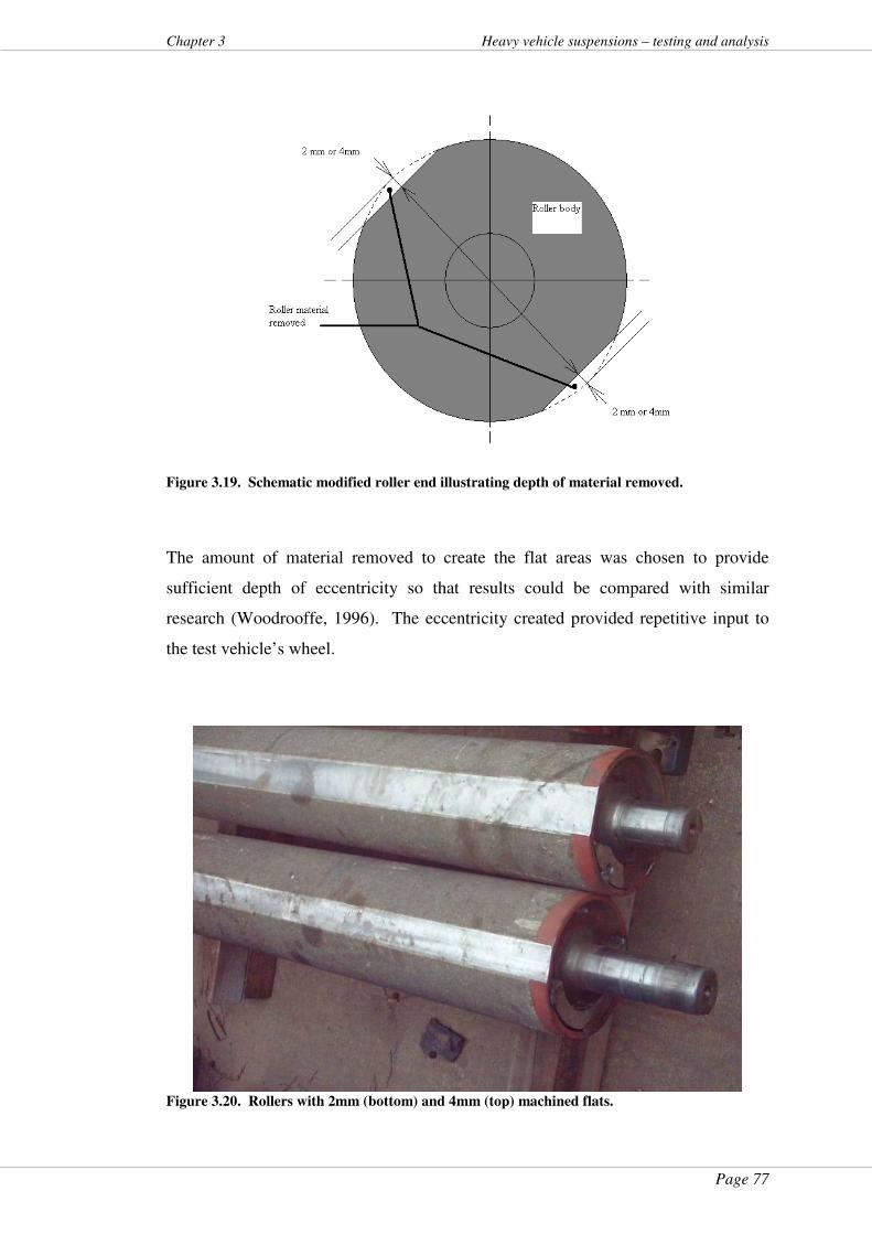
Page 77
Chapter 3 Heavy vehicle suspensions – testing and analysis
Figure 3.19. Schematic modified roller end illustrating depth of material removed.
The amount of material removed to create the flat areas was chosen to provide
sufficient depth of eccentricity so that results could be compared with similar
research (Woodrooffe, 1996). The eccentricity created provided repetitive input to
the test vehicle’s wheel.
Figure 3.20. Rollers with 2mm (bottom) and 4mm (top) machined flats.
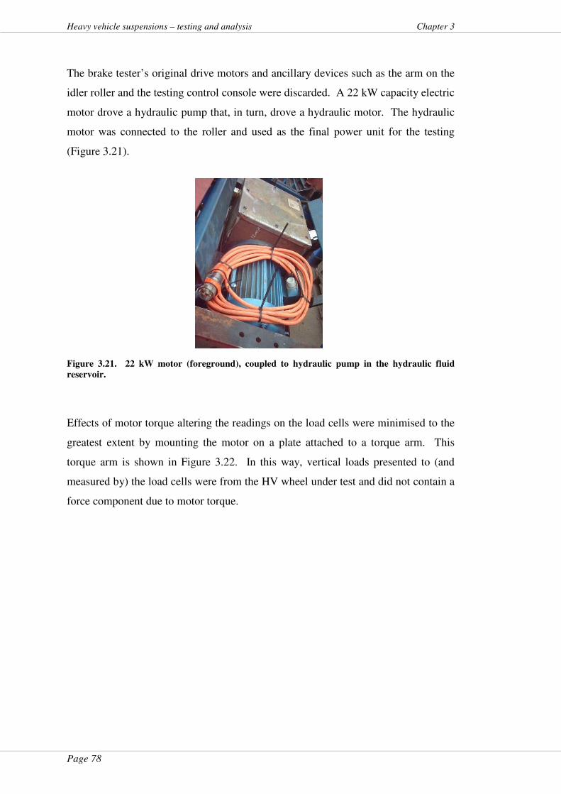
Page 78
Heavy vehicle suspensions – testing and analysis Chapter 3
The brake tester’s original drive motors and ancillary devices such as the arm on the
idler roller and the testing control console were discarded. A 22 kW capacity electric
motor drove a hydraulic pump that, in turn, drove a hydraulic motor. The hydraulic
motor was connected to the roller and used as the final power unit for the testing
(Figure 3.21).
Figure 3.21. 22 kW motor (foreground), coupled to hydraulic pump in the hydraulic fluid
reservoir.
Effects of motor torque altering the readings on the load cells were minimised to the
greatest extent by mounting the motor on a plate attached to a torque arm. This
torque arm is shown in Figure 3.22. In this way, vertical loads presented to (and
measured by) the load cells were from the HV wheel under test and did not contain a
force component due to motor torque.
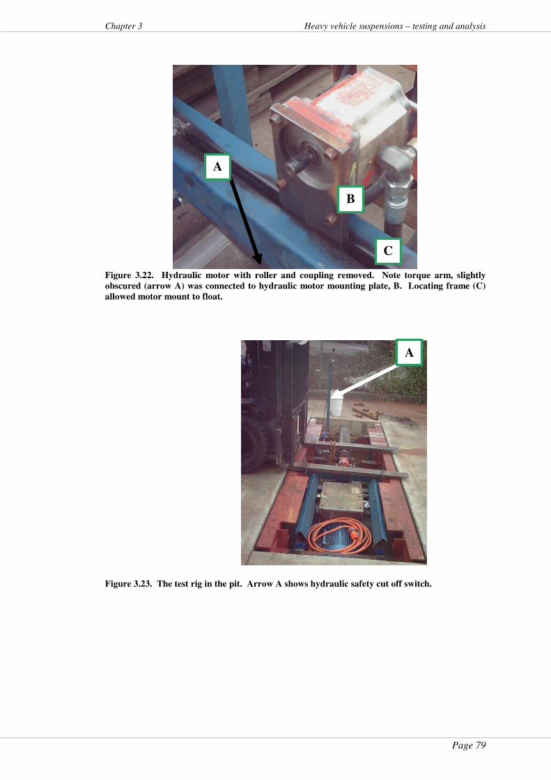
Page 79
Chapter 3 Heavy vehicle suspensions – testing and analysis
Figure 3.22. Hydraulic motor with roller and coupling removed. Note torque arm, slightly
obscured (arrow A) was connected to hydraulic motor mounting plate, B. Locating frame (C)
allowed motor mount to float.
Figure 3.23. The test rig in the pit. Arrow A shows hydraulic safety cut off switch.
A
A
B
C
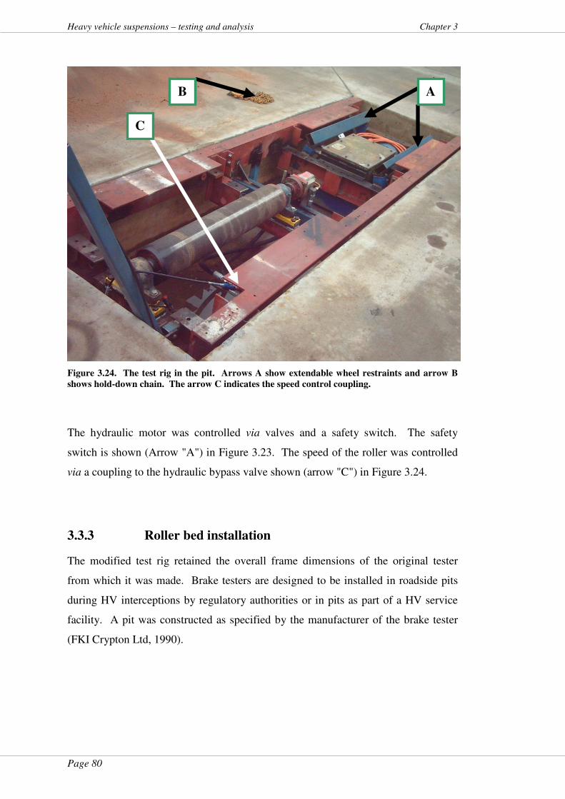
Page 80
Heavy vehicle suspensions – testing and analysis Chapter 3
Figure 3.24. The test rig in the pit. Arrows A show extendable wheel restraints and arrow B
shows hold-down chain. The arrow C indicates the speed control coupling.
The hydraulic motor was controlled via valves and a safety switch. The safety
switch is shown (Arrow "A") in Figure 3.23. The speed of the roller was controlled
via a coupling to the hydraulic bypass valve shown (arrow "C") in Figure 3.24.
3.3.3 Roller bed installation
The modified test rig retained the overall frame dimensions of the original tester
from which it was made. Brake testers are designed to be installed in roadside pits
during HV interceptions by regulatory authorities or in pits as part of a HV service
facility. A pit was constructed as specified by the manufacturer of the brake tester
(FKI Crypton Ltd, 1990).
C
A B
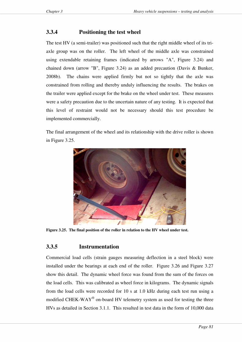
Page 81
Chapter 3 Heavy vehicle suspensions – testing and analysis
3.3.4 Positioning the test wheel
The test HV (a semi-trailer) was positioned such that the right middle wheel of its tri-
axle group was on the roller. The left wheel of the middle axle was constrained
using extendable retaining frames (indicated by arrows "A", Figure 3.24) and
chained down (arrow "B", Figure 3.24) as an added precaution (Davis & Bunker,
2008b). The chains were applied firmly but not so tightly that the axle was
constrained from rolling and thereby unduly influencing the results. The brakes on
the trailer were applied except for the brake on the wheel under test. These measures
were a safety precaution due to the uncertain nature of any testing. It is expected that
this level of restraint would not be necessary should this test procedure be
implemented commercially.
The final arrangement of the wheel and its relationship with the drive roller is shown
in Figure 3.25.
Figure 3.25. The final position of the roller in relation to the HV wheel under test.
3.3.5 Instrumentation
Commercial load cells (strain gauges measuring deflection in a steel block) were
installed under the bearings at each end of the roller. Figure 3.26 and Figure 3.27
show this detail. The dynamic wheel force was found from the sum of the forces on
the load cells. This was calibrated as wheel force in kilograms. The dynamic signals
from the load cells were recorded for 10 s at 1.0 kHz during each test run using a
modified CHEK-WAY® on-board HV telemetry system as used for testing the three
HVs as detailed in Section 3.1.1. This resulted in test data in the form of 10,000 data
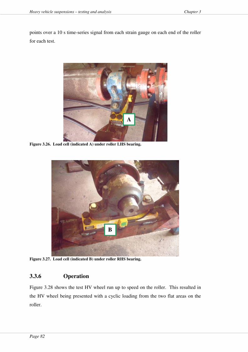
Page 82
Heavy vehicle suspensions – testing and analysis Chapter 3
points over a 10 s time-series signal from each strain gauge on each end of the roller
for each test.
Figure 3.26. Load cell (indicated A) under roller LHS bearing.
Figure 3.27. Load cell (indicated B) under roller RHS bearing.
3.3.6 Operation
Figure 3.28 shows the test HV wheel run up to speed on the roller. This resulted in
the HV wheel being presented with a cyclic loading from the two flat areas on the
roller.
A
B
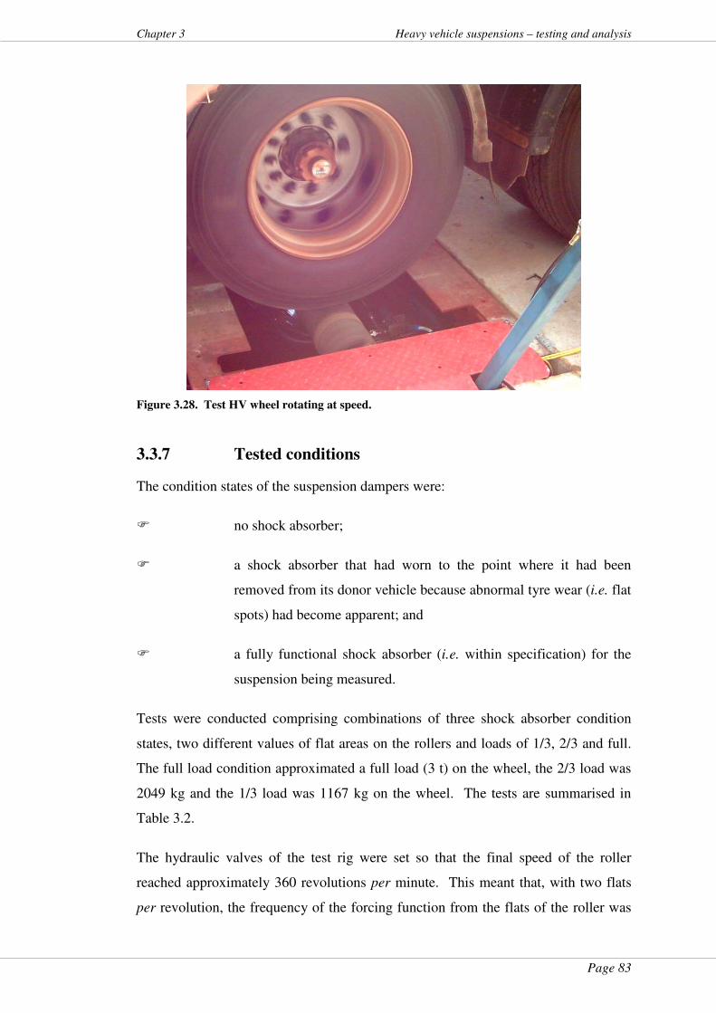
Page 83
Chapter 3 Heavy vehicle suspensions – testing and analysis
Figure 3.28. Test HV wheel rotating at speed.
3.3.7 Tested conditions
The condition states of the suspension dampers were:
� no shock absorber;
� a shock absorber that had worn to the point where it had been
removed from its donor vehicle because abnormal tyre wear (i.e. flat
spots) had become apparent; and
� a fully functional shock absorber (i.e. within specification) for the
suspension being measured.
Tests were conducted comprising combinations of three shock absorber condition
states, two different values of flat areas on the rollers and loads of 1/3, 2/3 and full.
The full load condition approximated a full load (3 t) on the wheel, the 2/3 load was
2049 kg and the 1/3 load was 1167 kg on the wheel. The tests are summarised in
Table 3.2.
The hydraulic valves of the test rig were set so that the final speed of the roller
reached approximately 360 revolutions per minute. This meant that, with two flats
per revolution, the frequency of the forcing function from the flats of the roller was
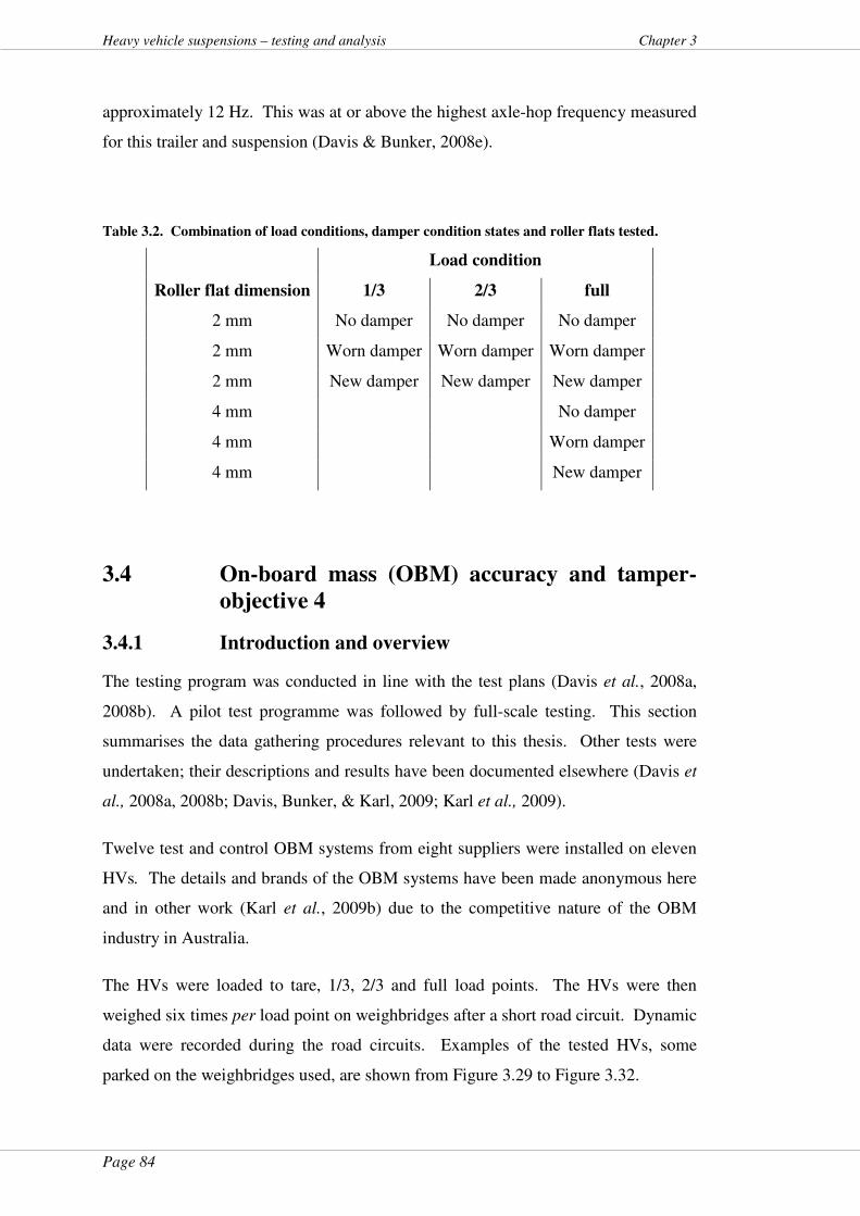
Page 84
Heavy vehicle suspensions – testing and analysis Chapter 3
approximately 12 Hz. This was at or above the highest axle-hop frequency measured
for this trailer and suspension (Davis & Bunker, 2008e).
Table 3.2. Combination of load conditions, damper condition states and roller flats tested.
Load condition
Roller flat dimension 1/3 2/3 full
2 mm No damper No damper No damper
2 mm Worn damper Worn damper Worn damper
2 mm New damper New damper New damper
4 mm No damper
4 mm Worn damper
4 mm New damper
3.4 On-board mass (OBM) accuracy and tamper-
objective 4
3.4.1 Introduction and overview
The testing program was conducted in line with the test plans (Davis et al., 2008a,
2008b). A pilot test programme was followed by full-scale testing. This section
summarises the data gathering procedures relevant to this thesis. Other tests were
undertaken; their descriptions and results have been documented elsewhere (Davis et
al., 2008a, 2008b; Davis, Bunker, & Karl, 2009; Karl et al., 2009).
Twelve test and control OBM systems from eight suppliers were installed on eleven
HVs. The details and brands of the OBM systems have been made anonymous here
and in other work (Karl et al., 2009b) due to the competitive nature of the OBM
industry in Australia.
The HVs were loaded to tare, 1/3, 2/3 and full load points. The HVs were then
weighed six times per load point on weighbridges after a short road circuit. Dynamic
data were recorded during the road circuits. Examples of the tested HVs, some
parked on the weighbridges used, are shown from Figure 3.29 to Figure 3.32.

Page 85
Chapter 3 Heavy vehicle suspensions – testing and analysis
Figure 3.29. Test HV –small road train.
Figure 3.30. Test HV – detail of small road train trailers.
Figure 3.31. Test HV – truck and dog trailer on weighbridge with similar combination
following.
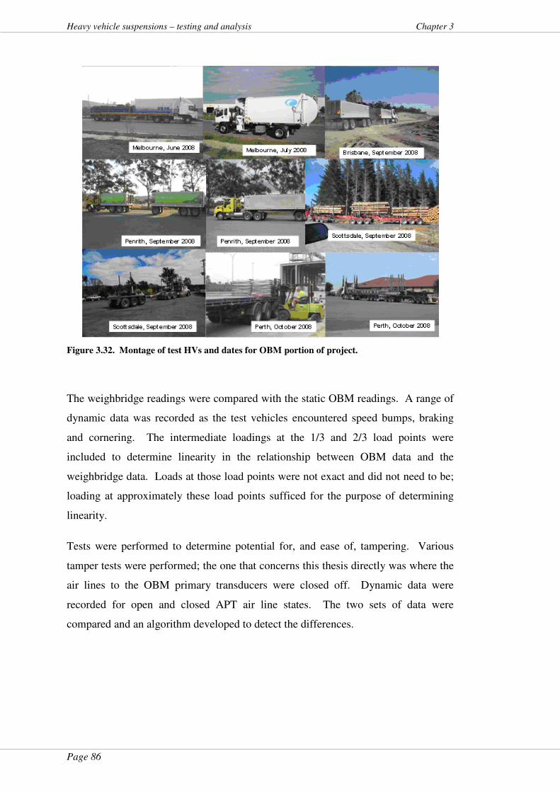
Page 86
Heavy vehicle suspensions – testing and analysis Chapter 3
Figure 3.32. Montage of test HVs and dates for OBM portion of project.
The weighbridge readings were compared with the static OBM readings. A range of
dynamic data was recorded as the test vehicles encountered speed bumps, braking
and cornering. The intermediate loadings at the 1/3 and 2/3 load points were
included to determine linearity in the relationship between OBM data and the
weighbridge data. Loads at those load points were not exact and did not need to be;
loading at approximately these load points sufficed for the purpose of determining
linearity.
Tests were performed to determine potential for, and ease of, tampering. Various
tamper tests were performed; the one that concerns this thesis directly was where the
air lines to the OBM primary transducers were closed off. Dynamic data were
recorded for open and closed APT air line states. The two sets of data were
compared and an algorithm developed to detect the differences.
Page 87
Chapter 3 Heavy vehicle suspensions – testing and analysis
3.4.2 Sampling frequency
It was postulated that dynamic data could inform the development of a tamper
indicator. Further to this, it was theorised that signal frequencies of the pressure in
the air springs and influenced by axle-hop would be key to this development.
As noted in Chapter 3, Section 3.1.1 and subsequently, HV axle-hop occurs at
frequencies of up to 15 Hz; periodicity 66.7 ms (Cebon, 1999). For the Nyquist
sampling criterion (Shannon’s theorem, Chapter 2, Section 2.3.3) to be satisfied, data
capture needed to be at least twice the frequency of interest (Houpis & Lamont,
1985) or at least 30 Hz; periodicity 33.3 ms.
Most commercial OBM systems do not record dynamic data at frequencies that
would have allowed axle-hop to be recorded but most manufacturers have stated that
their systems would be capable of such measurement, were it required (Davis, 2008).
Accordingly, data for use in Objective 4 were recorded using a HV OBM system
whose manufacturer had specified a sample interval of 24.0 ms, providing a
sampling rate of 41.6 Hz (Davis et al., 2008a, 2008b). As outlined in the background
theory for dynamic data sampling (Chapter 2, Section 2.3.3) this sampling frequency
was more than adequate to capture the test signal data since 41.6 Hz was higher than
the 30 Hz value derived from twice axle-hop. Accordingly, the Nyquist sampling
criterion (Shannon’s theorem) was met (Houpis & Lamont, 1985) for the testing.
3.4.3 Procedural detail
Each OBM system tested had a data set recorded for that unit. These data sets were
measured against a weighbridge or certified scales.
As a cross-validation of the data set from each test OBM, particularly for the
dynamic data recorded, another set of data was recorded. These data were recorded
by systems that were universal for all tests, regardless of vehicle. The data from
these systems provided sets of static and dynamic control data. Two OBM systems
common to all the tests and vehicles were used and were termed the reference OBM
systems. One of them recorded static and dynamic data contemporaneously with the
OBM system under test. The other recorded static data only. One outcome of the
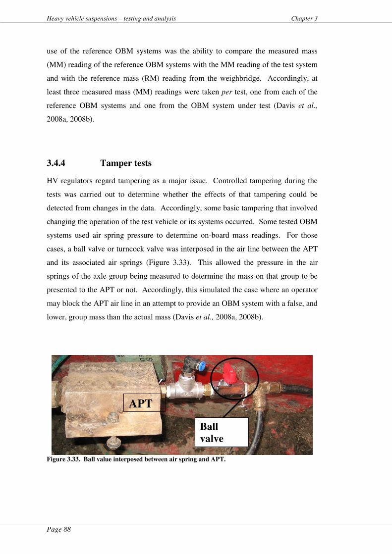
Page 88
Heavy vehicle suspensions – testing and analysis Chapter 3
use of the reference OBM systems was the ability to compare the measured mass
(MM) reading of the reference OBM systems with the MM reading of the test system
and with the reference mass (RM) reading from the weighbridge. Accordingly, at
least three measured mass (MM) readings were taken per test, one from each of the
reference OBM systems and one from the OBM system under test (Davis et al.,
2008a, 2008b).
3.4.4 Tamper tests
HV regulators regard tampering as a major issue. Controlled tampering during the
tests was carried out to determine whether the effects of that tampering could be
detected from changes in the data. Accordingly, some basic tampering that involved
changing the operation of the test vehicle or its systems occurred. Some tested OBM
systems used air spring pressure to determine on-board mass readings. For those
cases, a ball valve or turncock valve was interposed in the air line between the APT
and its associated air springs (Figure 3.33). This allowed the pressure in the air
springs of the axle group being measured to determine the mass on that group to be
presented to the APT or not. Accordingly, this simulated the case where an operator
may block the APT air line in an attempt to provide an OBM system with a false, and
lower, group mass than the actual mass (Davis et al., 2008a, 2008b).
Figure 3.33. Ball value interposed between air spring and APT.
APT
Ball
valve
Page 89
Chapter 3 Heavy vehicle suspensions – testing and analysis
3.4.5 Sample size
For each load condition, viz: tare, 1/3, 2/3 and full load; data readings were taken a
number of times to improve the reliability and accuracy of the results.
The sample size was determined from the process outlined in Appendix 3 and
summarised here.
A 95 percent level of confidence was chosen. Reasonable assumptions about:
� an experimental error value; and
� the spread of measurements from the population of OBM systems,
led to six readings per load condition. This meant six readings of the reference mass
(RM) and the measured mass (MM) per test load condition without changing any
other variables.
3.4.6 Exercising the HV suspensions
The suspensions of the tested HVs were exercised between readings to ensure that
influences due to bushing hysteresis, inter-leaf friction and air bag stretch, etc., were
averaged out over the readings. That meant that each test HV was required to
perform some travel activity before returning to be weighed again, typically a circuit
around a suburban block or within a transport depot.
3.5 Summary and conclusions of this chapter
This chapter has set down the background philosophy, methodology and choices
made in the experimental designs for the parts of the projects involved in preparation
of this thesis.
Some of the areas explored by the objectives and aims of this project were not
mainstream. A distinction needs to be made, however, between that which was
being tested and the methods used to test it. Ultimately, the data gathered involved
exercising the test HV in question and recording the data. Wherever a choice needed
Page 90
Heavy vehicle suspensions – testing and analysis Chapter 3
to be made between unproven or conservative methodology, the latter was chosen.
This methodology was then applied to the experimental design that provided the data
used in this thesis.
Where stochastic influences were foreseen in the experimental design, such as those
experienced with weighing devices (i.e. on-board mass measurement systems or
weighbridges), appropriate sample population numbers were developed using mature
methodology (Dubes, 1968; Snedecor & Cochran, 1967).
Likewise, conservative and proven methodology was chosen to determine wheel
forces from the experimental HVs (de Pont, 1997; Woodrooffe et al., 1986).
3.6 Chapter close
This chapter has described the procedures used for the testing and data gathering,
including (and/or referenced in Appendices) the conditions and rationale surrounding
each method.
Data thus gathered were analysed to:
� evaluate systems such as the “Haire suspension system” in Chapter
10 by making use of HV suspension metrics from Chapter 2 and the
roughness measures derived in Chapter 7;
� validate computer models in Chapter 5 after development of those
models in Chapter 4, noting that vertical acceleration data at the
hubs of interest and the concomitant air spring responses form the
input and output data for those models;
� evaluate variations in the load-sharing ability of computer models
from Chapter 4 and Chapter 5 to propose further improvements in
HV suspension designs in Chapter 12, Section 12.2.4 and Chapter
13, Section 13.3.1; and
� characterise on-board mass measurement systems in Chapter 8 and
develop and validate algorithms for OBM tamper-evidence in
Page 91
Chapter 3 Heavy vehicle suspensions – testing and analysis
Chapter 9.
That data and the models developed will then be used, amongst other outcomes, to
propose an in-service HV suspension health regime in Chapter 11 by a fusion of
OBM implementation and low-cost methodology for HV suspension testing.
Links where this chapter informs other chapters of this thesis are shown in Figure
1.4.
“There are two possible outcomes: if the result confirms the hypothesis, then you've made a measurement. If the result is contrary to the hypothesis, then you've made a
discovery.”- Enrico Fermi.

Page 92
Heavy vehicle suspensions – testing and analysis Chapter 4
4 Development of heavy vehicle suspension
models
4.1 About this chapter
This chapter details the development of heavy vehicle (HV) suspension models used
later in this thesis. Further, this chapter contains linkages between those models and
actual HV suspensions tested and described in Section 3.2. This work will be used to
address Objectives 1 to 3 in the areas of dynamic load sharing and in-service
suspension testing. This chapter then allows the scene to be set for validation of the
theoretical models, analysis of their outputs and conclusions drawn therefrom in
Chapter 6, particularly when correlated to actual HV suspension test data gathered as
detailed in Chapter 3.
4.2 Dynamic load sharing
4.2.1 Suspension model
Figure 4.1 presents a simple theoretical model that may assist to explore the concept
of dynamic load sharing between wheels or axles in a HV. The wheels, axles, etc. on
one axle in Figure 4.1 are assumed to be of equal mass to their corresponding
equivalent component on the other axle.
Let us consider Figure 4.1 in the context of a connection mechanism using
conventionally sized or “industry standard” longitudinal air lines which have
dimensions of approximately 4 to 12 mm inside diameter. Such a design does not
allow transfer of air between the air springs quickly enough when either of the
wheels encounters a bump at typical HV operating speeds (Blanksby et al., 2008a;
Davis & Sack, 2004; Simmons, 2005). This configuration may be considered to
exhibit no dynamic load sharing; therefore, its axles may be considered independent
of each other. Should one wheel encounter a non-uniformity of large enough
magnitude, were tyre elasticity not able to accommodate it; the other wheel could be
lifted off the ground momentarily. This would transfer the group mass to the wheel
still in contact with the road at that moment.
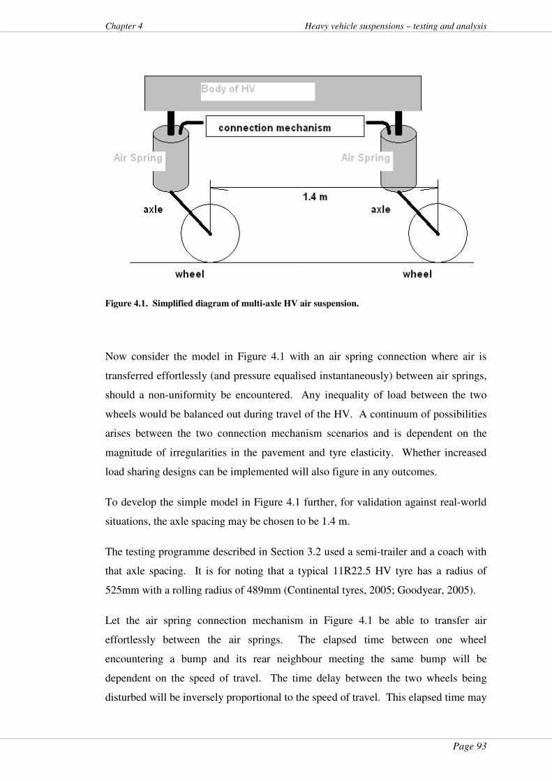
Page 93
Chapter 4 Heavy vehicle suspensions – testing and analysis
Figure 4.1. Simplified diagram of multi-axle HV air suspension.
Now consider the model in Figure 4.1 with an air spring connection where air is
transferred effortlessly (and pressure equalised instantaneously) between air springs,
should a non-uniformity be encountered. Any inequality of load between the two
wheels would be balanced out during travel of the HV. A continuum of possibilities
arises between the two connection mechanism scenarios and is dependent on the
magnitude of irregularities in the pavement and tyre elasticity. Whether increased
load sharing designs can be implemented will also figure in any outcomes.
To develop the simple model in Figure 4.1 further, for validation against real-world
situations, the axle spacing may be chosen to be 1.4 m.
The testing programme described in Section 3.2 used a semi-trailer and a coach with
that axle spacing. It is for noting that a typical 11R22.5 HV tyre has a radius of
525mm with a rolling radius of 489mm (Continental tyres, 2005; Goodyear, 2005).
Let the air spring connection mechanism in Figure 4.1 be able to transfer air
effortlessly between the air springs. The elapsed time between one wheel
encountering a bump and its rear neighbour meeting the same bump will be
dependent on the speed of travel. The time delay between the two wheels being
disturbed will be inversely proportional to the speed of travel. This elapsed time may
Page 94
Heavy vehicle suspensions – testing and analysis Chapter 4
be designated:
t = d / v Equation 4.1
where:
v = speed in ms-1;
d = distance in m; and
t = time in s.
The time constant of a system thus modelled may be represented as the difference in
time between the events of the two wheels encountering the same bump. In any
system, the time constant may also be defined as the inverse of the fundamental (or
resonant) frequency of the system.
The modes of vibration and frequencies of axles and bodies of HVs have been
documented extensively (Cebon, 1999; Davis & Bunker, 2008a, 2008e; de Pont,
1997). Providing the wheels and other rotating parts are balanced and suspension
components such as wheel bearings and shock absorbers are in good order, axle-hop
will occur when a wheel encounters a discontinuity in the road surface. Such an
impulse will start axle-hop that is characterized by a series of reducing excursions of
the wheel. Axle-hop frequencies occur in the range 10 to 15 Hz and, as speeds
increase, tend to the same order of magnitude as those of body bounce frequencies
(Davis & Bunker, 2008e). How quickly axle-hop excursions reduce will be a
function of suspension damper health and design characteristic (Section 2.3.1). For
the model in Figure 4.1, axle-hop forces would be transmitted along the connection
mechanism by the air spring first encountering a bump. These would be passed, in a
series of pneumatic pulses, to the rear air spring via the connection mechanism.
Shock absorbers in good condition should damp out this vibration but not before the
second air spring received a series of pressure impulses at the axle-hop frequency
common to both axles.
The time between these events for 1.4 m axle spacing would depend on travel speed
(Equation 4.1) and is shown in Table 4.1.
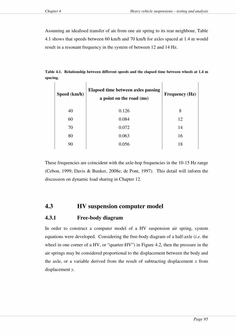
Page 95
Chapter 4 Heavy vehicle suspensions – testing and analysis
Assuming an idealised transfer of air from one air spring to its rear neighbour, Table
4.1 shows that speeds between 60 km/h and 70 km/h for axles spaced at 1.4 m would
result in a resonant frequency in the system of between 12 and 14 Hz.
Table 4.1. Relationship between different speeds and the elapsed time between wheels at 1.4 m
spacing.
Speed (km/h) Elapsed time between axles passing
a point on the road (ms) Frequency (Hz)
40 0.126 8
60 0.084 12
70 0.072 14
80 0.063 16
90 0.056 18
These frequencies are coincident with the axle-hop frequencies in the 10-15 Hz range
(Cebon, 1999; Davis & Bunker, 2008e; de Pont, 1997). This detail will inform the
discussion on dynamic load sharing in Chapter 12.
4.3 HV suspension computer model
4.3.1 Free-body diagram
In order to construct a computer model of a HV suspension air spring, system
equations were developed. Considering the free-body diagram of a half-axle (i.e. the
wheel in one corner of a HV, or “quarter-HV”) in Figure 4.2, then the pressure in the
air springs may be considered proportional to the displacement between the body and
the axle, or a variable derived from the result of subtracting displacement x from
displacement y.
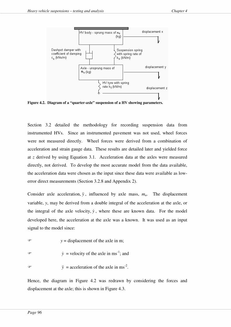
Page 96
Heavy vehicle suspensions – testing and analysis Chapter 4
Figure 4.2. Diagram of a “quarter-axle” suspension of a HV showing parameters.
Section 3.2 detailed the methodology for recording suspension data from
instrumented HVs. Since an instrumented pavement was not used, wheel forces
were not measured directly. Wheel forces were derived from a combination of
acceleration and strain gauge data. These results are detailed later and yielded force
at z derived by using Equation 3.1. Acceleration data at the axles were measured
directly, not derived. To develop the most accurate model from the data available,
the acceleration data were chosen as the input since these data were available as low-
error direct measurements (Section 3.2.8 and Appendix 2).
Consider axle acceleration, y&& , influenced by axle mass, mu. The displacement
variable, y, may be derived from a double integral of the acceleration at the axle, or
the integral of the axle velocity, y& , where these are known data. For the model
developed here, the acceleration at the axle was a known. It was used as an input
signal to the model since:
� y = displacement of the axle in m;
� y& = velocity of the axle in ms-1; and
� y&& = acceleration of the axle in ms-2.
Hence, the diagram in Figure 4.2 was redrawn by considering the forces and
displacement at the axle; this is shown in Figure 4.3.
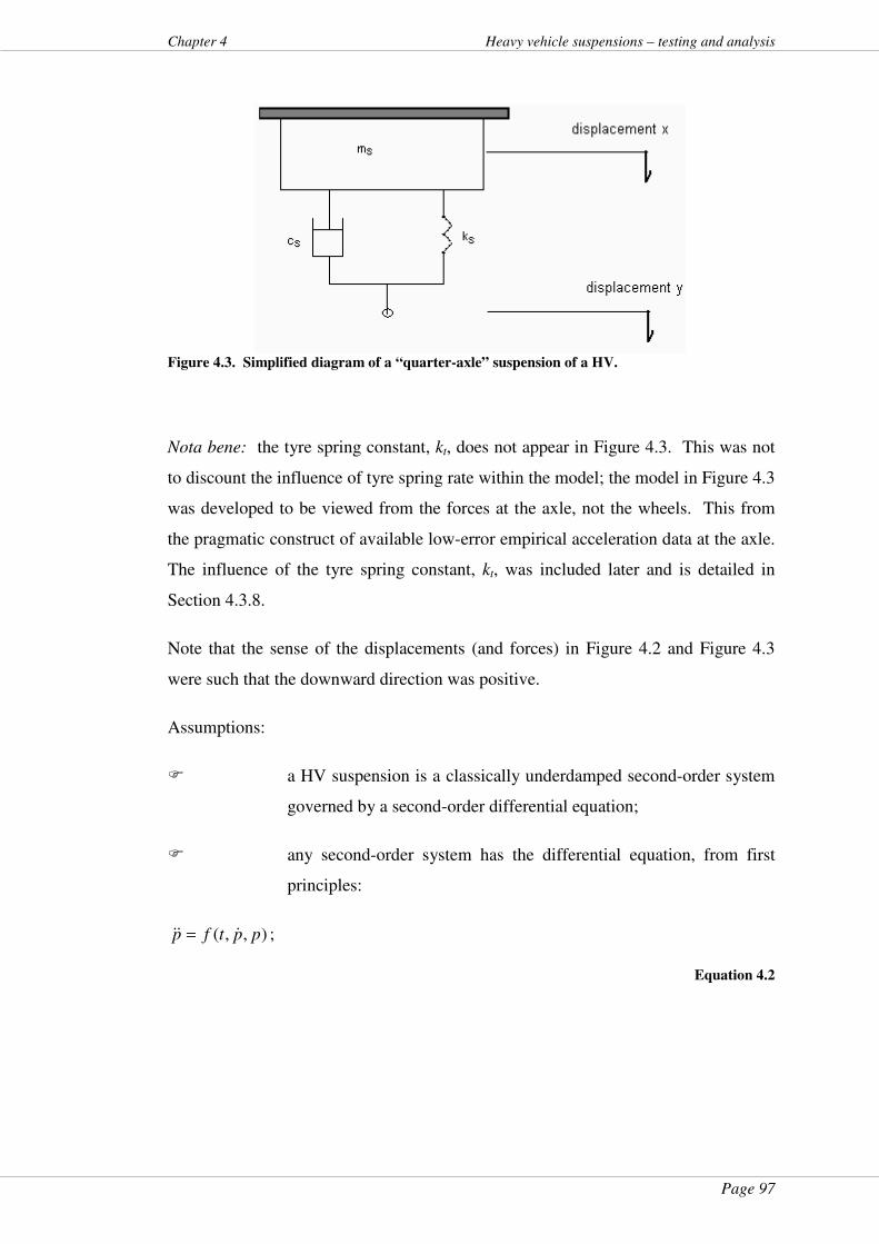
Page 97
Chapter 4 Heavy vehicle suspensions – testing and analysis
Figure 4.3. Simplified diagram of a “quarter-axle” suspension of a HV.
Nota bene: the tyre spring constant, kt, does not appear in Figure 4.3. This was not
to discount the influence of tyre spring rate within the model; the model in Figure 4.3
was developed to be viewed from the forces at the axle, not the wheels. This from
the pragmatic construct of available low-error empirical acceleration data at the axle.
The influence of the tyre spring constant, kt, was included later and is detailed in
Section 4.3.8.
Note that the sense of the displacements (and forces) in Figure 4.2 and Figure 4.3
were such that the downward direction was positive.
Assumptions:
� a HV suspension is a classically underdamped second-order system
governed by a second-order differential equation;
� any second-order system has the differential equation, from first
principles:
),,( pptfp &&& = ;
Equation 4.2
Page 98
Heavy vehicle suspensions – testing and analysis Chapter 4
and the generalised system equation for such a body with damping (Meriam &
Kraige, 1993) is:
kppcpm ++ &&& = 0
Equation 4.3
where:
m is the mass of the body;
c is the damping coefficient;
k is the spring rate;
and p is the time-dependent system response.
Applying the generalised system equation, Equation 4.3, to the free-body diagram in
Figure 4.3, some detailed assumptions may reasonably be made:
� the system equation for the free-body diagram in Figure 4.3 for the
sprung mass is: xkxcxm sss ++ &&& = 0;
� the spring rate, ks, is linear regardless of direction;
� the damping coefficient, cs, varies piecewise-linearly according to
direction of movement (Costanzi & Cebon, 2005, 2006; Duym,
Stiens, & Reybrouck, 1997; Prem et al., 1998; Uffelmann & Walter,
1994);
� bushings, locating rods or other suspension components add no
differential spring action, dead-band or hysteresis; and
� the springs and the dampers do not reach their limits of travel (i.e.
no spring or damper hysteresis; no “bang-bang” limiting).
These assumptions were proven valid as detailed later (Chapter 5); should they not
have been, they would have been revisited.
Page 99
Chapter 4 Heavy vehicle suspensions – testing and analysis
4.3.2 Regarding spring rate linearity and the damping
characteristic
Modelling of HV suspensions that included air springs with non-linear spring rates
over the entire range of spring travel has been carried out (Costanzi & Cebon, 2005,
2006). That work involved complex modelling and allocated some hysteresis to the
springs at the limits of air spring travel (Costanzi & Cebon, 2005, 2006). However,
Costanzi and Cebon (2005, 2006) noted that air spring hysteresis occurred over a
very small portion of the overall range. Other researchers have produced less
complex models of HVs suspensions that were used for pavement damage research
(Cole & Cebon, 2007; Prem et al., 1998). Those models ascribed a linear value to
the spring rate, ks. Accordingly, for the models used in this thesis, linear spring rates
were chosen. Manufacturer’s data (Mack-Volvo, 2007b) and the previous work on
simple-to-moderately complex HV suspension models justified this assumption.
The moderately complex models of HV suspensions used for pavement damage
research and development of HV suspension designs used models with a piece-wise
linear damping coefficient, cs, which varied depending on direction (Cole & Cebon,
2007; Duym et al., 1997; Prem et al., 1998). Even the complex modelling of
Costanzi and Cebon (2005, 2006) assumed linear, but unequal, damping coefficients
in either direction. For the models used in this thesis, piecewise-linear damping
coefficients were derived for damper bounce and rebound cases.
These assumptions were proven valid as detailed later (Chapter 5); should they not
have been, they would have been revisited.
4.3.3 System equations
Newton’s Second Law and Newtonian mechanics allowed a system equation to be
developed using the relationship that the axle has with the body of the HV in Figure
4.3 as follows:
Newton’s Second Law states:
onacceleratimassForce ×= Equation 4.4
Page 100
Heavy vehicle suspensions – testing and analysis Chapter 4
The first force to consider on the body of the HV in Figure 4.3 is due to its mass and
acceleration; using Equation 4.4:
xmForce s&&= mass) sprung theofon accelerati and mass to(due
Equation 4.5
where:
ms = sprung mass of the HV; and
x&& = acceleration at the body of the HV.
Now consider the spatial relationship that the body and the axle have with respect to
each other. That relationship may be defined by the forces on the components in
Figure 4.3. The force on a damper is proportional to the relative velocities between
its ends as defined by its damping coefficient, cs. From Figure 4.3, this force may be
described as:
)( yxcforceDamper s&& −= .
Equation 4.6
where cs = damping coefficient of the shock absorber;
x& = velocity of the body of the HV; and
y& = velocity of the axle.
The spring force is defined by its spring rate, ks, and is proportional to the relative
displacement between its two ends. From Figure 4.3, this force may be described as:
)( yxkforceSpring s −=
Equation 4.7
where ks = spring rate;
x = displacement of the body of the HV; and
y = displacement of the axle.
The sum of the total force ( )(totalForce ) on the HV body in Figure 4.3 may be found
Page 101
Chapter 4 Heavy vehicle suspensions – testing and analysis
by adding the forces found from Equation 4.5, Equation 4.6 and Equation 4.7:
)()()()( yxkyxcxmForce ssstotal −+−+= &&&&
Equation 4.8
from Newtonian mechanics, the forces on a body may be summed to zero (Meriam &
Kraige, 1993):
0)( =totalForce
Equation 4.9
since the HV body exhibits second-order underdamped behaviour, Equation 4.8 and
Equation 4.9 may be equated and re-written:
)()()()( yxkyxcxmForce ssstotal −+−+= &&&& = 0
Equation 4.10
From Equation 4.10 therefore:
)()()( yxkyxcxm sss −+−+ &&&& = 0
Equation 4.11
=> 0)()( =−+−+ yxkyxcxm sss&&&&
=> )()()( xykxycxm sss −+−= &&&&
Equation 4.12
and restating the variables and their units:
� ms = the mass of the body in kg;
� cs = the damping coefficient (nota bene: not the damping ratio) of
the shock absorber in kNs/m;
� ks = the spring constant in kN/m;
� y = displacement of the axle in m;
� y& = velocity of the axle in m.s-1;
� x = displacement of the body in m;
� x& = velocity of the body in m.s-1; and
Page 102
Heavy vehicle suspensions – testing and analysis Chapter 4
� x&& = acceleration of the body in m.s-2.
Equation 4.12 shows that the forces on the body are created by the forces from the
shock absorber and the spring combined. This equation was used to develop the
computer models used in the following sections and in Chapter 5.
4.3.4 Damped natural frequency
Assuming underdamped behaviour, with some justification from empirical evidence
(Davis & Bunker, 2008a; Davis, Kel, & Sack, 2007; Davis & Sack, 2004, 2006), the
equation of motion from an underdamped second-order system equation provided the
relationship between the undamped natural frequency, nω , the damped natural
frequency, dω , and the damping ratio, ζ (defined in Section 4.3.5):
nω =21 ζ
ω
−
d
Equation 4.13
where:
� dω = the damped natural frequency; or body bounce frequency, in
rad.s-1;
� nω = undamped natural frequency; and
� ζ = the damping ratio (Meriam & Kraige, 1993; Thomson & Dahleh, 1998).
The damped natural frequency, f, is the inverse of the time (period) between
successive points on the output waveform (e.g. successive peaks or successive zero-
crossings) of a second-order system response to an impulse input. Figure 4.4 shows
this time as Td.
From first principles:
π
ω
2
1 d
dTf == ;
Equation 4.14
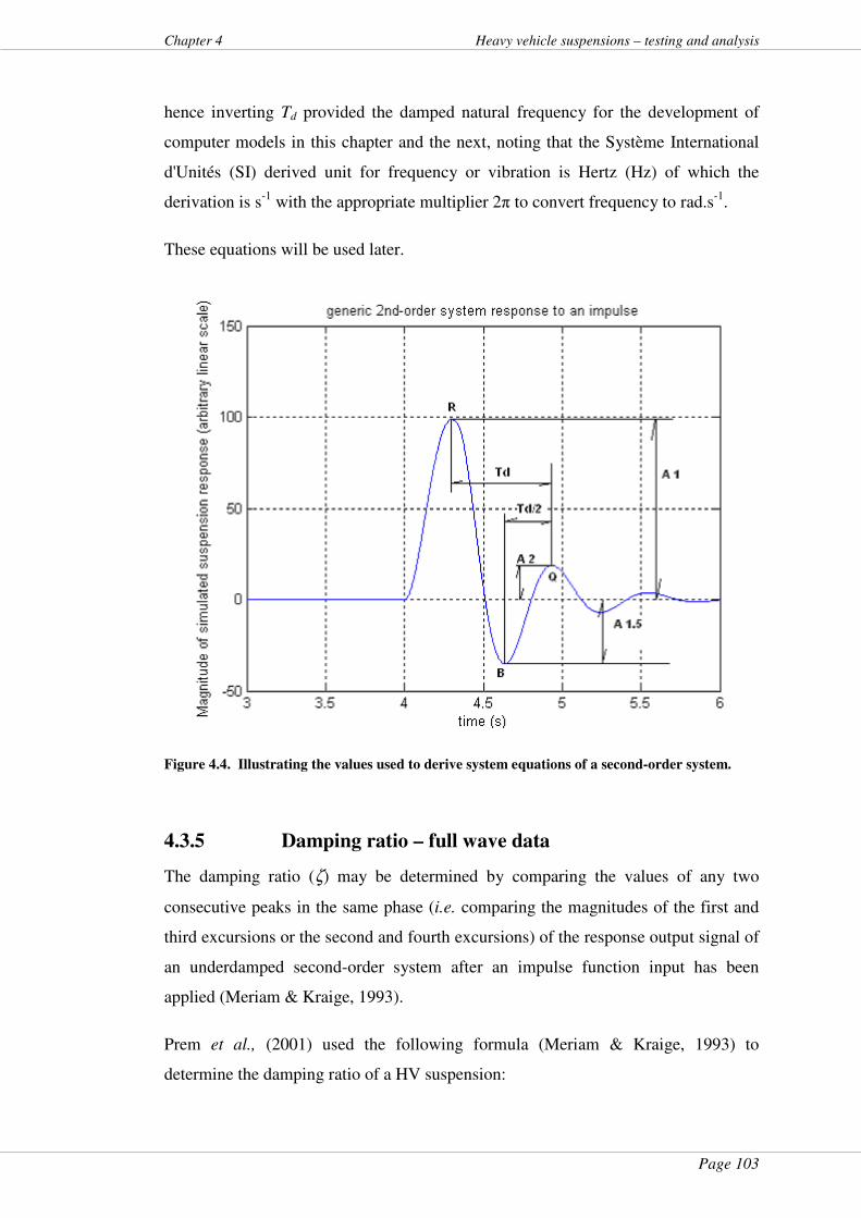
Page 103
Chapter 4 Heavy vehicle suspensions – testing and analysis
hence inverting Td provided the damped natural frequency for the development of
computer models in this chapter and the next, noting that the Système International
d'Unités (SI) derived unit for frequency or vibration is Hertz (Hz) of which the
derivation is s-1 with the appropriate multiplier 2π to convert frequency to rad.s-1.
These equations will be used later.
Figure 4.4. Illustrating the values used to derive system equations of a second-order system.
4.3.5 Damping ratio – full wave data
The damping ratio (ζ) may be determined by comparing the values of any two
consecutive peaks in the same phase (i.e. comparing the magnitudes of the first and
third excursions or the second and fourth excursions) of the response output signal of
an underdamped second-order system after an impulse function input has been
applied (Meriam & Kraige, 1993).
Prem et al., (2001) used the following formula (Meriam & Kraige, 1993) to
determine the damping ratio of a HV suspension:
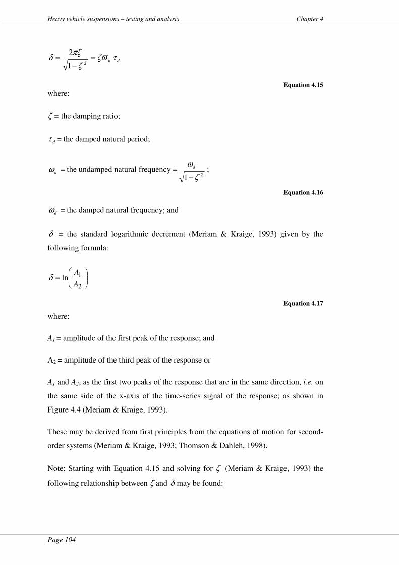
Page 104
Heavy vehicle suspensions – testing and analysis Chapter 4
dn τζϖζ
πζδ =
−=
21
2
Equation 4.15
where:
ζ = the damping ratio;
dτ = the damped natural period;
nω = the undamped natural frequency =21 ζ
ω
−
d ;
Equation 4.16
dω = the damped natural frequency; and
δ = the standard logarithmic decrement (Meriam & Kraige, 1993) given by the
following formula:
=
2
1lnA
Aδ
Equation 4.17
where:
A1 = amplitude of the first peak of the response; and
A2 = amplitude of the third peak of the response or
A1 and A2, as the first two peaks of the response that are in the same direction, i.e. on
the same side of the x-axis of the time-series signal of the response; as shown in
Figure 4.4 (Meriam & Kraige, 1993).
These may be derived from first principles from the equations of motion for second-
order systems (Meriam & Kraige, 1993; Thomson & Dahleh, 1998).
Note: Starting with Equation 4.15 and solving for ζ (Meriam & Kraige, 1993) the
following relationship between ζ and δ may be found:

Page 105
Chapter 4 Heavy vehicle suspensions – testing and analysis
Equation 4.18
as shown in other work (Davis & Bunker, 2007).
4.3.6 Damping ratio – half wave data
Where a half-cycle of the response from a second-order system to an impulse is
available, the half-cycle damping ratio may be found by using:
� the first two peaks: A1, A1.5; and
� half the damped natural period 2
dτ;
from those variables, as shown in Figure 4.4.
Hence the period between A1 and A1.5 is half the damped natural period or2
dτ.
The damping ratio from a half-wave signal, 2/1δ , may be derived from the same
equations of motion used to derive the full-wave damping ratio above by restating
Equation 4.15 (Thomson & Dahleh, 1998):
21
2
ζ
πζτζϖδ
−= = dn
Equation 4.19
then substituting
2
dτ for the period and adjusting the other sides of the equation for
equality:
22/1
12 ζ
πζτζϖδ
−= = d
n
Equation 4.20
where:
ζ = damping ratio;
])2[( 22 δπδζ +=
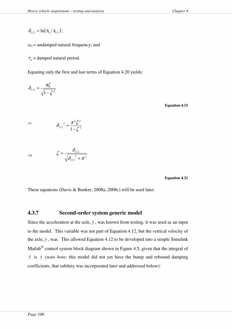
Page 106
Heavy vehicle suspensions – testing and analysis Chapter 4
( )5.112/1 ln AA=δ ;
ωn = undamped natural frequency; and
dτ = damped natural period.
Equating only the first and last terms of Equation 4.20 yields:
22/1
1 ζ
πζδ
−=
Equation 4.15
⇒
⇒
Equation 4.21
These equations (Davis & Bunker, 2008a, 2008c) will be used later.
4.3.7 Second-order system generic model
Since the acceleration at the axle, y&& , was known from testing, it was used as an input
to the model. This variable was not part of Equation 4.12, but the vertical velocity of
the axle, y& , was. This allowed Equation 4.12 to be developed into a simple Simulink
Matlab control system block diagram shown in Figure 4.5, given that the integral of
y&& is y& (nota bene: this model did not yet have the bump and rebound damping
coefficients, that subtlety was incorporated later and addressed below):
2
222
2/11 ζ
ζπδ
−=
22
2/1
2/1
πδ
δζ
+=
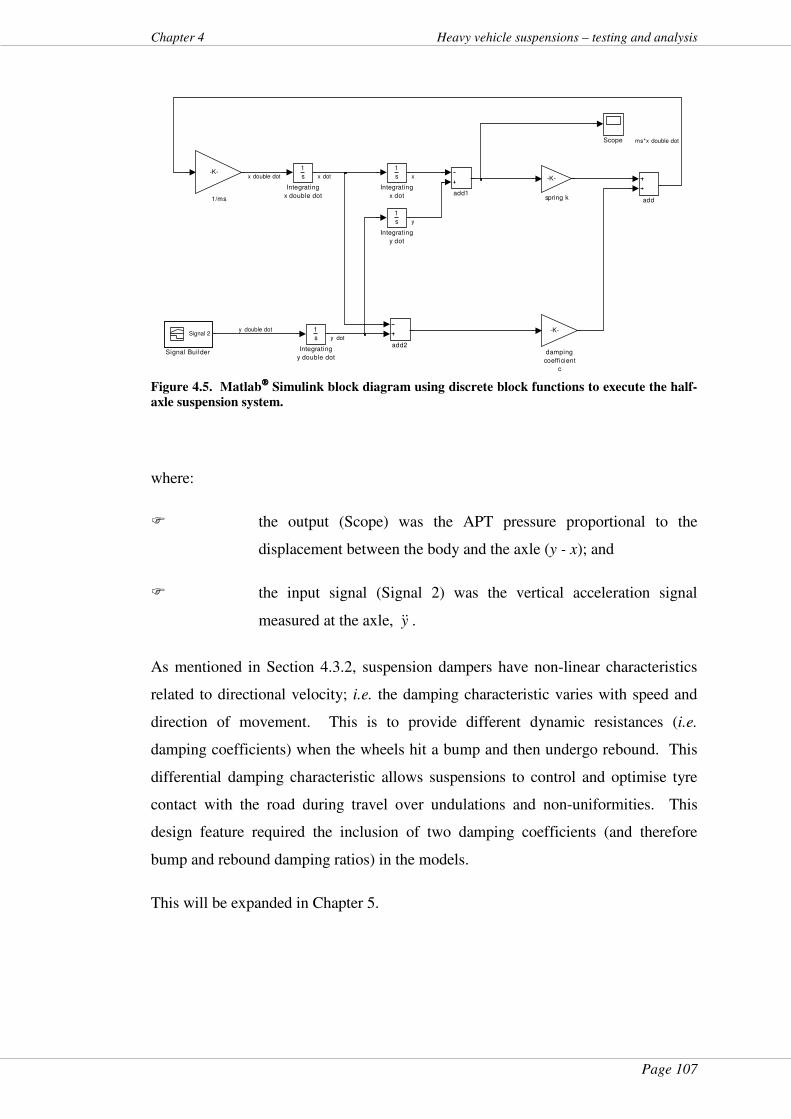
Page 107
Chapter 4 Heavy vehicle suspensions – testing and analysis
-K-
spring k
-K-
damping
coefficient
c
add2
add1add
Signal 2
Signal Builder
Scope
1
s
Integrating
y double dot
1
s
Integrating
y dot
1
s
Integrating
x double dot
1
s
Integrating
x dot
-K-
1/ms
y double dot
ms*x double dot
y
xx double dot x dot
y dot
Figure 4.5. Matlab
Simulink block diagram using discrete block functions to execute the half-
axle suspension system.
where:
� the output (Scope) was the APT pressure proportional to the
displacement between the body and the axle (y - x); and
� the input signal (Signal 2) was the vertical acceleration signal
measured at the axle, y&& .
As mentioned in Section 4.3.2, suspension dampers have non-linear characteristics
related to directional velocity; i.e. the damping characteristic varies with speed and
direction of movement. This is to provide different dynamic resistances (i.e.
damping coefficients) when the wheels hit a bump and then undergo rebound. This
differential damping characteristic allows suspensions to control and optimise tyre
contact with the road during travel over undulations and non-uniformities. This
design feature required the inclusion of two damping coefficients (and therefore
bump and rebound damping ratios) in the models.
This will be expanded in Chapter 5.
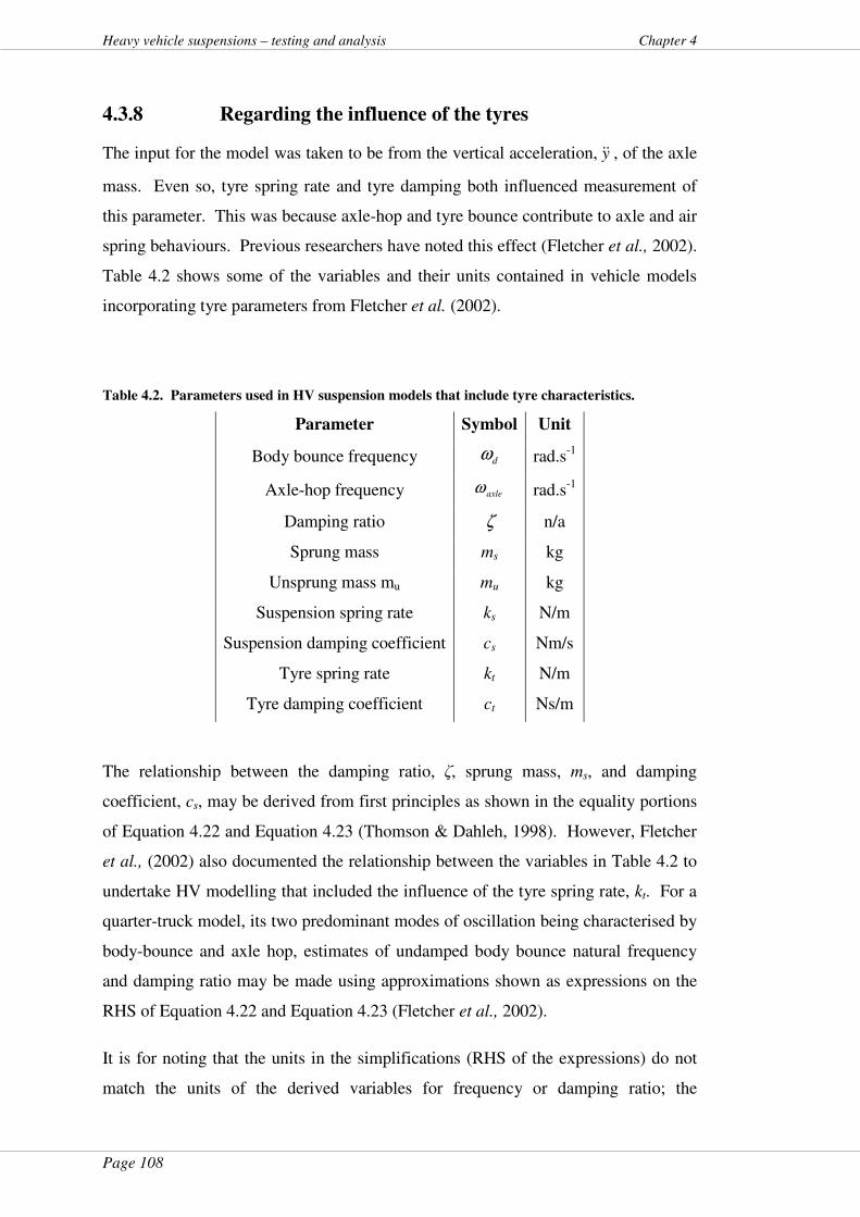
Page 108
Heavy vehicle suspensions – testing and analysis Chapter 4
4.3.8 Regarding the influence of the tyres
The input for the model was taken to be from the vertical acceleration, y&& , of the axle
mass. Even so, tyre spring rate and tyre damping both influenced measurement of
this parameter. This was because axle-hop and tyre bounce contribute to axle and air
spring behaviours. Previous researchers have noted this effect (Fletcher et al., 2002).
Table 4.2 shows some of the variables and their units contained in vehicle models
incorporating tyre parameters from Fletcher et al. (2002).
Table 4.2. Parameters used in HV suspension models that include tyre characteristics.
Parameter Symbol Unit
Body bounce frequency dω rad.s-1
Axle-hop frequency axleω rad.s-1
Damping ratio ζ n/a
Sprung mass ms kg
Unsprung mass mu mu kg
Suspension spring rate ks N/m
Suspension damping coefficient cs Nm/s
Tyre spring rate kt N/m
Tyre damping coefficient ct Ns/m
The relationship between the damping ratio, ζ, sprung mass, ms, and damping
coefficient, cs, may be derived from first principles as shown in the equality portions
of Equation 4.22 and Equation 4.23 (Thomson & Dahleh, 1998). However, Fletcher
et al., (2002) also documented the relationship between the variables in Table 4.2 to
undertake HV modelling that included the influence of the tyre spring rate, kt. For a
quarter-truck model, its two predominant modes of oscillation being characterised by
body-bounce and axle hop, estimates of undamped body bounce natural frequency
and damping ratio may be made using approximations shown as expressions on the
RHS of Equation 4.22 and Equation 4.23 (Fletcher et al., 2002).
It is for noting that the units in the simplifications (RHS of the expressions) do not
match the units of the derived variables for frequency or damping ratio; the
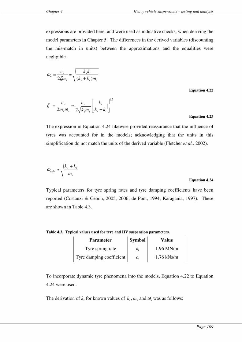
Page 109
Chapter 4 Heavy vehicle suspensions – testing and analysis
expressions are provided here, and were used as indicative checks, when deriving the
model parameters in Chapter 5. The differences in the derived variables (discounting
the mis-match in units) between the approximations and the equalities were
negligible.
sts
ts
s
s
nmkk
kk
m
c
)(2 +≈=
ζω
Equation 4.22
5.1
22
+≈=
ts
t
ss
s
ns
s
kk
k
mk
c
m
c
ωζ
Equation 4.23
The expression in Equation 4.24 likewise provided reassurance that the influence of
tyres was accounted for in the models; acknowledging that the units in this
simplification do not match the units of the derived variable (Fletcher et al., 2002).
u
ts
axlem
kk +≈ω
Equation 4.24
Typical parameters for tyre spring rates and tyre damping coefficients have been
reported (Costanzi & Cebon, 2005, 2006; de Pont, 1994; Karagania, 1997). These
are shown in Table 4.3.
Table 4.3. Typical values used for tyre and HV suspension parameters.
Parameter Symbol Value
Tyre spring rate kt 1.96 MN/m
Tyre damping coefficient ct 1.76 kNs/m
To incorporate dynamic tyre phenomena into the models, Equation 4.22 to Equation
4.24 were used.
The derivation of ks for known values of nst mk ω and , was as follows:
Page 110
Heavy vehicle suspensions – testing and analysis Chapter 4
=> sts
ts
s
sn
mkk
kk
m
c
)(2 +≈=
ζω
Equation 4.22
=> 2
2
nst
nst
smk
mkk
ω
ω
−≈
Equation 4.25
Provided the damped natural frequency, damping ratio and mass of a HV suspension
were known, the damping coefficient, cs, could be derived for the model in Figure
4.5 from a re-stated Equation 4.23 (Thomson & Dahleh, 1998):
=>
5.1
22
+≈=
ts
t
ss
s
ns
s
kk
k
mk
c
m
c
ωζ
Equation 4.23
=> 5.1
22
+
≈=
ts
t
ss
nss
kk
k
mkmc
ζωζ
Equation 4.26
From the spring rate, ks, found from Equation 4.25 and a known value of damping
ratio, ζ, from either Equation 4.18 or Equation 4.21, Equation 4.26 provided both the
generalised damping coefficient values and the bump and rebound damping
coefficients for the models developed in the next chapter. Accordingly, contributory
components from tyre influence on the variables ks and cs (Figure 4.5) were
incorporated into the models.
4.4 Summary and conclusions of this chapter
Computer simulations were necessary for completion of this project and thesis. This
was because performing variations in parameters on live suspensions would have
been risky to personnel and possibly destructive to tested HVs. Accordingly,
simulations were performed using computer models as analogues of HV suspensions.
To create those models, system equations governing second-order underdamped
systems were theorised. Relationships between the various components of HV
suspensions were gathered from known sources. By applying a combination of those
system equations and known HV suspension characteristics, a generic computer

Page 111
Chapter 4 Heavy vehicle suspensions – testing and analysis
model was developed. This chapter has documented the fundamentals upon which
the development of that generic computer model was based.
4.5 Chapter close
Two models have been developed in this chapter. The first, a simple model of two
axles will allow exploration of dynamic load sharing. The second, a computer
simulation model, was developed in generic form. This generic computer model will
allow the data gathered from HV testing (Section 3.2) to be developed into three
separate analogues of the HVs axles tested. Individual models for each HV axle will
allow empirical data to be input with analysis of the associated outputs to be detailed
in Chapters 5 and 6.
Accordingly, these models will inform the discussion regarding:
� the efficacy of systems such as the “Haire suspension system”
(Objective 2) from analysis (Chapters 10, 12 and 13);
� in-service suspension testing (Objective 3) of air-sprung HVs in
Chapter 6; and
� implications of increased dynamic load sharing (Chapters 10, 12 and
13).
Links where this chapter informs other chapters of this thesis are shown in Figure
1.4.
“All models are flawed – some are useful.” - W. Ed Deming.
Page 112
Heavy vehicle suspensions – testing and analysis Chapter 5
5 Heavy vehicle suspension model
calibration and validation
5.1 About this chapter
This chapter documents the development of the heavy vehicle (HV) suspension
computer model built up in the previous chapter. It shows the application of this
suspension model to the three test vehicles in Section 3.2. System equations detailed
in Chapter 4 and empirical data gathered as described in Section 3.2 were used to
determine parameters for three HV axle models. Validation of the models was then
undertaken by showing the results achieved when the computer model outputs were
compared with empirical outputs for the same input data. These models will be used
to meet Objective 2, dealing with dynamic load sharing, and Objective 3,
development of low-cost in-service HV suspension testing.
5.2 Introduction
The generic computer model developed in Chapter 4 was designed to have the
acceleration at the axle as the input signal and air spring pressure, being a surrogate
of the axle-to-body displacement, as the output signal. This matched a portion of the
data from the experimental design outlined in Section 3.2. This chapter documents
the analysis of input (accelerometer) and output (air spring) data signals from the
VSB 11-style step tests to determine suspension parameters for the three HVs tested
in Section 3.2. The various blocks in the computer model were then populated from
the relationship between those signals to develop three “quarter-HV” models. These
models were then calibrated against the VSB 11-style step test output data recorded
per test vehicle as described in Section 3.2. Once the computer model parameters
were determined, data from the accelerometers recorded during the VSB 11-style
step tests were input to the computer models. The output data from the models as
analogues for air spring responses were then compared with empirical results for air
spring data with those results documented in this chapter. A diagrammatic summary
of the process and how this chapter relates to, and uses data from, previous chapters
is illustrated in Figure 5.1.
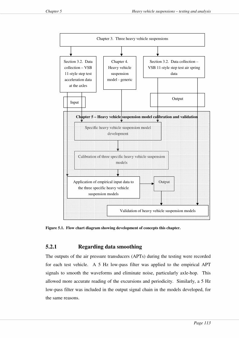
Page 113
Chapter 5 Heavy vehicle suspensions – testing and analysis
Figure 5.1. Flow chart diagram showing development of concepts this chapter.
5.2.1 Regarding data smoothing
The outputs of the air pressure transducers (APTs) during the testing were recorded
for each test vehicle. A 5 Hz low-pass filter was applied to the empirical APT
signals to smooth the waveforms and eliminate noise, particularly axle-hop. This
allowed more accurate reading of the excursions and periodicity. Similarly, a 5 Hz
low-pass filter was included in the output signal chain in the models developed, for
the same reasons.
Section 3.2. Data
collection – VSB
11-style step test
acceleration data
at the axles
Chapter 4.
Heavy vehicle
suspension
model - generic
Specific heavy vehicle suspension model
development
Section 3.2. Data collection –
VSB 11-style step test air spring
data
Input Output
Chapter 3. Three heavy vehicle suspensions
Calibration of three specific heavy vehicle suspension
models
Output
Chapter 5 – Heavy vehicle suspension model calibration and validation
Validation of heavy vehicle suspension models
Application of empirical input data to
the three specific heavy vehicle
suspension models
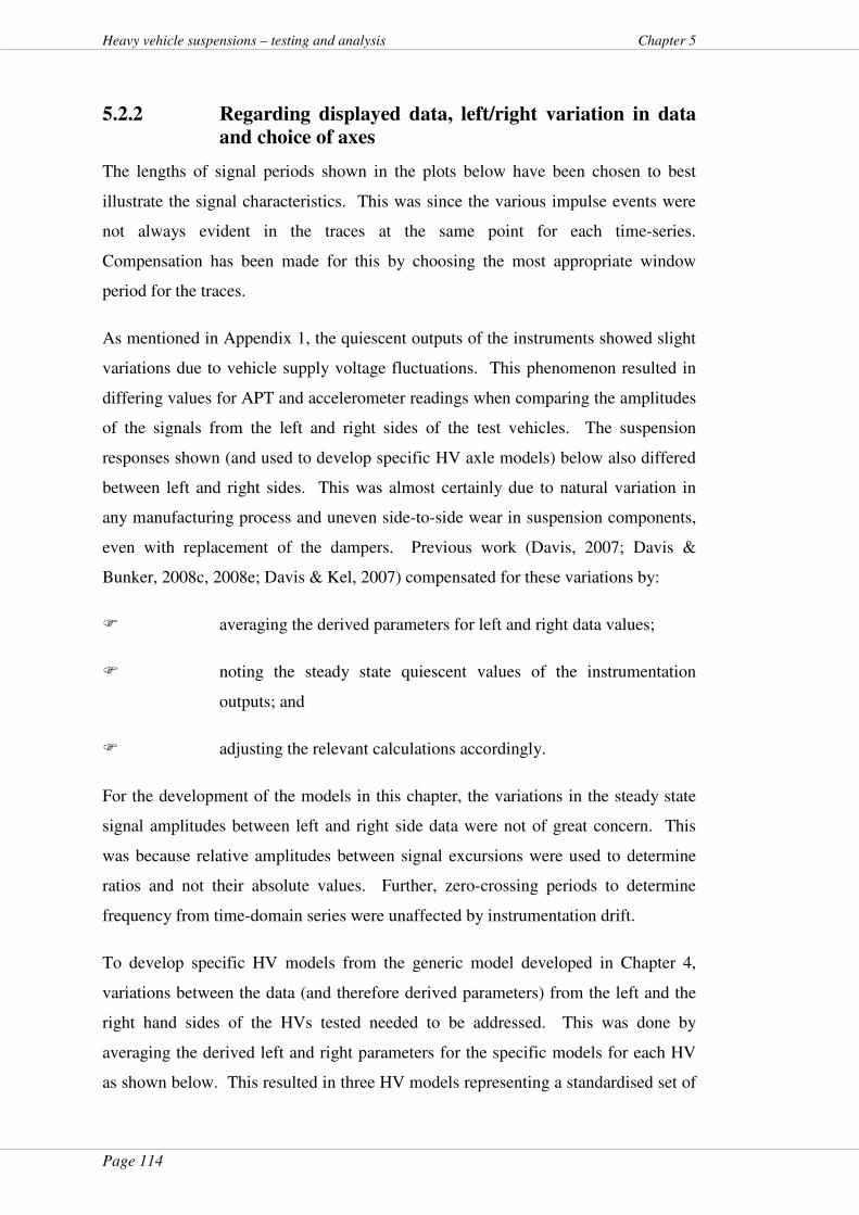
Page 114
Heavy vehicle suspensions – testing and analysis Chapter 5
5.2.2 Regarding displayed data, left/right variation in data
and choice of axes
The lengths of signal periods shown in the plots below have been chosen to best
illustrate the signal characteristics. This was since the various impulse events were
not always evident in the traces at the same point for each time-series.
Compensation has been made for this by choosing the most appropriate window
period for the traces.
As mentioned in Appendix 1, the quiescent outputs of the instruments showed slight
variations due to vehicle supply voltage fluctuations. This phenomenon resulted in
differing values for APT and accelerometer readings when comparing the amplitudes
of the signals from the left and right sides of the test vehicles. The suspension
responses shown (and used to develop specific HV axle models) below also differed
between left and right sides. This was almost certainly due to natural variation in
any manufacturing process and uneven side-to-side wear in suspension components,
even with replacement of the dampers. Previous work (Davis, 2007; Davis &
Bunker, 2008c, 2008e; Davis & Kel, 2007) compensated for these variations by:
� averaging the derived parameters for left and right data values;
� noting the steady state quiescent values of the instrumentation
outputs; and
� adjusting the relevant calculations accordingly.
For the development of the models in this chapter, the variations in the steady state
signal amplitudes between left and right side data were not of great concern. This
was because relative amplitudes between signal excursions were used to determine
ratios and not their absolute values. Further, zero-crossing periods to determine
frequency from time-domain series were unaffected by instrumentation drift.
To develop specific HV models from the generic model developed in Chapter 4,
variations between the data (and therefore derived parameters) from the left and the
right hand sides of the HVs tested needed to be addressed. This was done by
averaging the derived left and right parameters for the specific models for each HV
as shown below. This resulted in three HV models representing a standardised set of
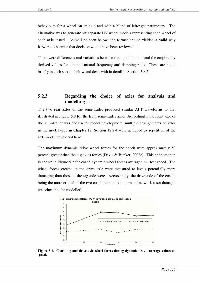
Page 115
Chapter 5 Heavy vehicle suspensions – testing and analysis
behaviours for a wheel on an axle and with a blend of left/right parameters. The
alternative was to generate six separate HV wheel models representing each wheel of
each axle tested. As will be seen below, the former choice yielded a valid way
forward, otherwise that decision would have been reviewed.
There were differences and variations between the model outputs and the empirically
derived values for damped natural frequency and damping ratio. These are noted
briefly in each section below and dealt with in detail in Section 5.8.2.
5.2.3 Regarding the choice of axles for analysis and
modelling
The two rear axles of the semi-trailer produced similar APT waveforms to that
illustrated in Figure 5.8 for the front semi-trailer axle. Accordingly, the front axle of
the semi-trailer was chosen for model development; multiple arrangements of axles
in the model used in Chapter 12, Section 12.2.4 were achieved by repetition of the
axle model developed here.
The maximum dynamic drive wheel forces for the coach were approximately 50
percent greater than the tag axles forces (Davis & Bunker, 2008e). This phenomenon
is shown in Figure 5.2 for coach dynamic wheel forces averaged per test speed. The
wheel forces created at the drive axle were measured at levels potentially more
damaging than those at the tag axle were. Accordingly, the drive axle of the coach,
being the more critical of the two coach rear axles in terms of network asset damage,
was chosen to be modelled.
Peak dynamic wheel force (PDWF) averaged per test speed - coach
loaded
2.0
3.0
4.0
5.0
6.0
7.0
8.0
9.0
10.0
11.0
40 50 60 70 80 90
Speed (km/h)
Max. w
heel fo
rce (
kN
/9.8
)
Std PDWF - tag Std PDWF - drive
Figure 5.2. Coach tag and drive axle wheel forces during dynamic tests – average values vs.
speed.
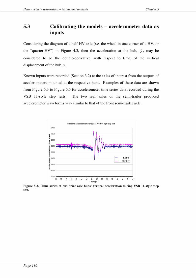
Page 116
Heavy vehicle suspensions – testing and analysis Chapter 5
5.3 Calibrating the models – accelerometer data as
inputs
Considering the diagram of a half-HV axle (i.e. the wheel in one corner of a HV, or
the “quarter-HV”) in Figure 4.3, then the acceleration at the hub, y&& , may be
considered to be the double-derivative, with respect to time, of the vertical
displacement of the hub, y.
Known inputs were recorded (Section 3.2) at the axles of interest from the outputs of
accelerometers mounted at the respective hubs. Examples of these data are shown
from Figure 5.3 to Figure 5.5 for accelerometer time series data recorded during the
VSB 11-style step tests. The two rear axles of the semi-trailer produced
accelerometer waveforms very similar to that of the front semi-trailer axle.
Bus drive axle accelerometer signal - VSB 11-style step test
2000
2050
2100
2150
2200
2250
2300
2350
2400
2.0
2.2
2.4
2.6
2.8
3.0
3.2
3.4
3.6
3.8
4.0
4.2
4.4
4.6
4.8
5.0
Time (s)
Ac
ce
lero
me
ter
ou
tpu
t (a
rbit
rary
lin
ea
r s
ca
le)
LEFT
RIGHT
Figure 5.3. Time series of bus drive axle hubs’ vertical acceleration during VSB 11-style step
test.
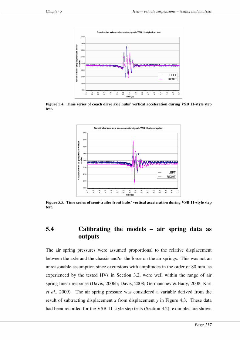
Page 117
Chapter 5 Heavy vehicle suspensions – testing and analysis
Coach drive axle accelerometer signal - VSB 11- style drop test
1900
2000
2100
2200
2300
2400
2500
2600
2700
2.0
2.2
2.4
2.6
2.8
3.0
3.2
3.4
3.6
3.8
4.0
4.2
4.4
4.6
4.8
5.0
Time (s)
Ac
ce
lero
me
ter
ou
tpu
t (a
rbit
rary
lin
ea
r
sc
ale
)
LEFT
RIGHT
Figure 5.4. Time series of coach drive axle hubs’ vertical acceleration during VSB 11-style step
test.
Semi-trailer front axle accelerometer signal - VSB 11-style step test
1900
2000
2100
2200
2300
2400
2500
2600
2700
4.0
4.2
4.4
4.6
4.8
5.0
5.2
5.4
5.6
5.8
6.0
6.2
6.4
6.6
6.8
7.0
Time (s)
Ac
ce
lero
me
ter
ou
tpu
t (a
rbit
rary
lin
ear
sc
ale
)
LEFT
RIGHT
Figure 5.5. Time series of semi-trailer front hubs’ vertical acceleration during VSB 11-style step
test.
5.4 Calibrating the models – air spring data as
outputs
The air spring pressures were assumed proportional to the relative displacement
between the axle and the chassis and/or the force on the air springs. This was not an
unreasonable assumption since excursions with amplitudes in the order of 80 mm, as
experienced by the tested HVs in Section 3.2, were well within the range of air
spring linear response (Davis, 2006b; Davis, 2008; Germanchev & Eady, 2008; Karl
et al., 2009). The air spring pressure was considered a variable derived from the
result of subtracting displacement x from displacement y in Figure 4.3. These data
had been recorded for the VSB 11-style step tests (Section 3.2); examples are shown

Page 118
Heavy vehicle suspensions – testing and analysis Chapter 5
from Figure 5.6 to Figure 5.8 for APT time series signals.
Bus drive axle APT signal - VSB 11-style step test
1700
1750
1800
1850
1900
1950
2000
2050
2100
3.0
3.2
3.4
3.6
3.8
4.0
4.2
4.4
4.6
4.8
5.0
5.2
5.4
5.6
5.8
6.0
6.2
6.4
6.6
6.8
7.0
7.2
7.4
7.6
7.8
8.0
Time (s)
AP
T o
utp
ut
(arb
itra
ry lin
ear
scale
)
LEFT
RIGHT
Figure 5.6. Time series of bus drive axle APT output during VSB 11-style step test.
Coach drive axle APT signal - VSB 11-style step test
1600
1700
1800
1900
2000
2100
2200
2.0
2.2
2.4
2.6
2.8
3.0
3.2
3.4
3.6
3.8
4.0
4.2
4.4
4.6
4.8
5.0
5.2
5.4
5.6
5.8
6.0
Time (s)
AP
T o
utp
ut
(arb
itra
ry lin
ear
sc
ale
)
LEFT
RIGHT
Figure 5.7. Time series of coach drive axle APT output during VSB 11-style step test.
These data were chosen as the reference cases for the three HVs tested, VSB 11
being the standard for “road friendliness” of HV suspensions (Australia Department
of Transport and Regional Services, 2004a, 2004c).
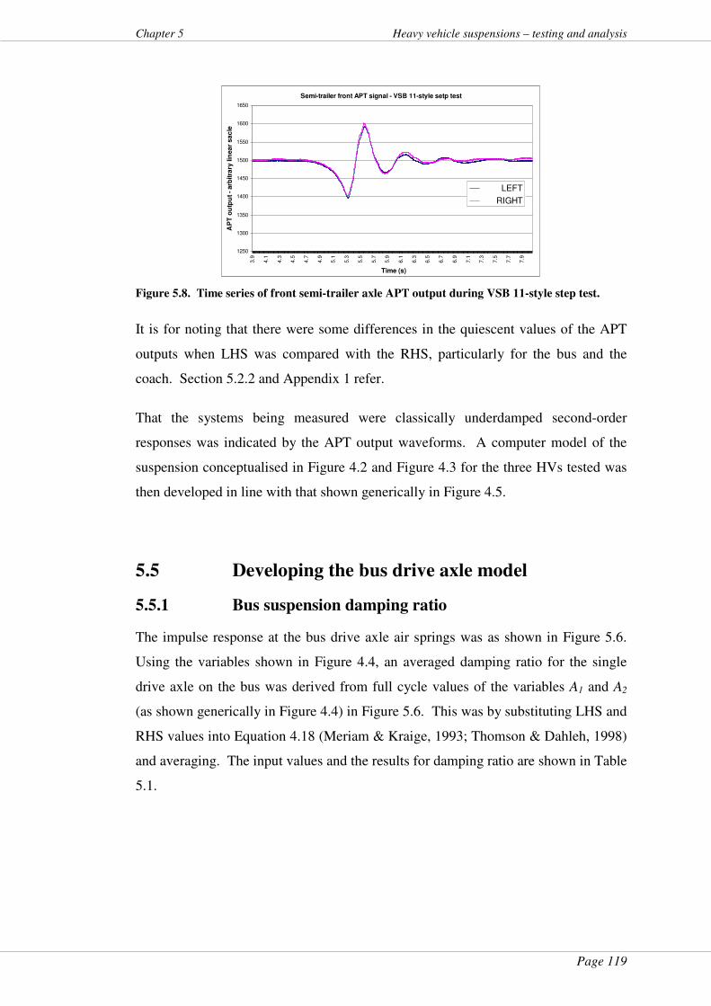
Page 119
Chapter 5 Heavy vehicle suspensions – testing and analysis
Semi-trailer front APT signal - VSB 11-style setp test
1250
1300
1350
1400
1450
1500
1550
1600
1650
3.9
4.1
4.3
4.5
4.7
4.9
5.1
5.3
5.5
5.7
5.9
6.1
6.3
6.5
6.7
6.9
7.1
7.3
7.5
7.7
7.9
Time (s)
AP
T o
utp
ut
- arb
itra
ry lin
ea
r s
ac
le
LEFT
RIGHT
Figure 5.8. Time series of front semi-trailer axle APT output during VSB 11-style step test.
It is for noting that there were some differences in the quiescent values of the APT
outputs when LHS was compared with the RHS, particularly for the bus and the
coach. Section 5.2.2 and Appendix 1 refer.
That the systems being measured were classically underdamped second-order
responses was indicated by the APT output waveforms. A computer model of the
suspension conceptualised in Figure 4.2 and Figure 4.3 for the three HVs tested was
then developed in line with that shown generically in Figure 4.5.
5.5 Developing the bus drive axle model
5.5.1 Bus suspension damping ratio
The impulse response at the bus drive axle air springs was as shown in Figure 5.6.
Using the variables shown in Figure 4.4, an averaged damping ratio for the single
drive axle on the bus was derived from full cycle values of the variables A1 and A2
(as shown generically in Figure 4.4) in Figure 5.6. This was by substituting LHS and
RHS values into Equation 4.18 (Meriam & Kraige, 1993; Thomson & Dahleh, 1998)
and averaging. The input values and the results for damping ratio are shown in Table
5.1.
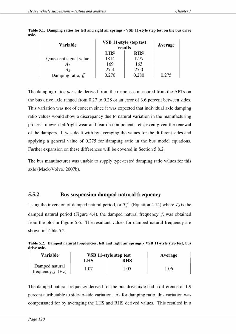
Page 120
Heavy vehicle suspensions – testing and analysis Chapter 5
Table 5.1. Damping ratios for left and right air springs - VSB 11-style step test on the bus drive
axle.
Variable VSB 11-style step test
results Average
LHS RHS Quiescent signal value 1814 1777
A1 169 163 A2 27.4 27.0
Damping ratio, ζ 0.270 0.280 0.275
The damping ratios per side derived from the responses measured from the APTs on
the bus drive axle ranged from 0.27 to 0.28 or an error of 3.6 percent between sides.
This variation was not of concern since it was expected that individual axle damping
ratio values would show a discrepancy due to natural variation in the manufacturing
process, uneven left/right wear and tear on components, etc; even given the renewal
of the dampers. It was dealt with by averaging the values for the different sides and
applying a general value of 0.275 for damping ratio in the bus model equations.
Further expansion on these differences will be covered in Section 5.8.2.
The bus manufacturer was unable to supply type-tested damping ratio values for this
axle (Mack-Volvo, 2007b).
5.5.2 Bus suspension damped natural frequency
Using the inversion of damped natural period, or 1−dT (Equation 4.14) where Td is the
damped natural period (Figure 4.4), the damped natural frequency, f, was obtained
from the plot in Figure 5.6. The resultant values for damped natural frequency are
shown in Table 5.2.
Table 5.2. Damped natural frequencies, left and right air springs - VSB 11-style step test, bus
drive axle.
Variable VSB 11-style step test Average
LHS RHS Damped natural
frequency, f (Hz) 1.07 1.05 1.06
The damped natural frequency derived for the bus drive axle had a difference of 1.9
percent attributable to side-to-side variation. As for damping ratio, this variation was
compensated for by averaging the LHS and RHS derived values. This resulted in a

Page 121
Chapter 5 Heavy vehicle suspensions – testing and analysis
damped natural frequency for the model of 1.06 Hz or 6.66 rad.s-1. The bus
manufacturer was unable to supply type-tested body-bounce frequency data for this
axle (Mack-Volvo, 2007b).
5.5.3 Bus suspension model variables
A computer model from the generalised diagram in Figure 4.5 was developed. To
populate the variables in Equation 4.12 as they applied to the bus, variation in
derived damping ratios between the two sides was compensated for by averaging the
LHS and the RHS damping ratio. The VSB 11-style step test provided an averaged
damping ratio value of 0.275 (Table 5.1). The damped natural body bounce
frequency, dω , for the model (Table 5.2) was 6.66 rad.s-1 (1.06 Hz) after averaging
the LHS and the RHS values. The undamped natural frequency for the model was
found from Equation 4.16 using a damping ratio, ζ, of 0.275, yielding an undamped
natural frequency, dω , of 6.93 rad.s-1 or 1.10 Hz. A sprung mass for the system
model, ms, of 4.47 t was derived from a measured wheel mass of 5 t (Davis &
Bunker, 2009e) less half the total unsprung mass of the bus axle being 530 kg (Prem,
2008).
Table 5.3 lists the totalised variables for the model after this process, those listed in
Table 4.3 and those derived from Equation 4.25 and Equation 4.26.
Table 5.3. Given and derived tyre and HV suspension parameters - bus.
Parameter Symbol Value Unit
Undamped natural body bounce frequency nω 6.93 rad.s-1
Sprung mass ms 4.47 t Unsprung mass mu 0.530 t
Suspension spring rate ks 239 kN/m Suspension damping coefficient cs 21.4 kNs/m
Tyre spring rate kt 1.96 MN/m
Axle-hop frequency axleω 10.2 Hz
Page 122
Heavy vehicle suspensions – testing and analysis Chapter 5
Manufacturer’s data were provided for a static spring rate, ks, range varying between
47.6 and 286 kN/m (Mack-Volvo, 2007a); the derived spring rate, ks, in Table 5.3
was within this range. The lower value of 47.6 kN/m was for tests at very small
excursions; a low incremental spring rate to provide a soft ride over small
perturbations.
As a check for the axle-hop frequency value derived here, fast Fourier transforms
(FFTs) of the accelerometer signal from the bus axle (in Figure 5.3) showed axle-hop
frequencies between 8.5 Hz and 10.8 Hz (Davis & Bunker, 2008e); 10.2 Hz was
within this range.
The bump and rebound damping ratios were determined from the excursions in the
positive and negative directions of the signals from the VSB 11-style step tests
(Figure 5.6). Figure 4.4 illustrates the starting points and conventions for derivation
of differing damping ratios, depending on the relative direction of movement
between the axle and the body. From Figure 4.4 and using Equation 4.21:
� the convention for the signal excursion from R to B was taken as the
case of rebound damping where the axle was moving away from the
chassis; and
� the signal excursion from B to Q was for the case of bump damping
where the axle was moving toward the chassis.
The damping ratios were determined for the cases of:
� bump, where the body and axle move toward each other. This
resulted in a positive sense for xy && − which, in turn, required the
model to recognise only positive values of xy && − (i.e. a lower limit
of zero for xy && − ). This limiting condition was applied to the
feedback loop controlling the bump damping coefficient; and
� rebound, where the body and axle move away from each other. This
resulted in negative values for xy && − which, in turn, required the
model to consider only the negative values of xy && − (i.e. an upper
limit of zero for xy && − ). This limiting condition was applied as the
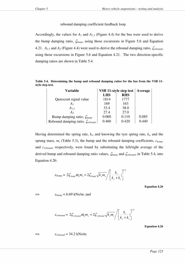
Page 123
Chapter 5 Heavy vehicle suspensions – testing and analysis
rebound damping coefficient feedback loop.
Accordingly, the values for A1 and A1.5 (Figure 4.4) for the bus were used to derive
the bump damping ratio, ζbump, using those excursions in Figure 5.6 and Equation
4.21. A1.5 and A2 (Figure 4.4) were used to derive the rebound damping ratio, ζrebound,
using those excursions in Figure 5.6 and Equation 4.21. The two direction-specific
damping ratios are shown in Table 5.4.
Table 5.4. Determining the bump and rebound damping ratios for the bus from the VSB 11-
style step test.
Variable VSB 11-style step test Average LHS RHS
Quiescent signal value 1814 1777 A1 169 163 A1.5 33.4 38.0 A2 27.4 27.0
Bump damping ratio, ζbump 0.060 0.110 0.085
Rebound damping ratio, ζrebound 0.460 0.420 0.440
Having determined the spring rate, ks, and knowing the tyre spring rate, kt, and the
sprung mass, ms (Table 5.3), the bump and the rebound damping coefficients, cbump,
and crebound, respectively, were found by substituting the left/right average of the
derived bump and rebound damping ratio values, ζbump, and ζrebound, in Table 5.4, into
Equation 4.26:
cbump =
5.1
22
+≈
ts
tssbumpsnbump
kk
kmkm ζωζ
Equation 4.26
=> cbump = 6.69 kNs/m; and
crebound =
5.1
22
+≈
ts
tssreboundsnrebound
kk
kmkm ζωζ
Equation 4.26
=> crebound = 34.2 kNs/m.
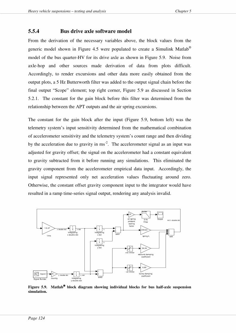
Page 124
Heavy vehicle suspensions – testing and analysis Chapter 5
5.5.4 Bus drive axle software model
From the derivation of the necessary variables above, the block values from the
generic model shown in Figure 4.5 were populated to create a Simulink Matlab
model of the bus quarter-HV for its drive axle as shown in Figure 5.9. Noise from
axle-hop and other sources made derivation of data from plots difficult.
Accordingly, to render excursions and other data more easily obtained from the
output plots, a 5 Hz Butterworth filter was added to the output signal chain before the
final output “Scope” element; top right corner, Figure 5.9 as discussed in Section
5.2.1. The constant for the gain block before this filter was determined from the
relationship between the APT outputs and the air spring excursions.
The constant for the gain block after the input (Figure 5.9, bottom left) was the
telemetry system’s input sensitivity determined from the mathematical combination
of accelerometer sensitivity and the telemetry system’s count range and then dividing
by the acceleration due to gravity in ms-2. The accelerometer signal as an input was
adjusted for gravity offset; the signal on the accelerometer had a constant equivalent
to gravity subtracted from it before running any simulations. This eliminated the
gravity component from the accelerometer empirical data input. Accordingly, the
input signal represented only net acceleration values fluctuating around zero.
Otherwise, the constant offset gravity component input to the integrator would have
resulted in a ramp time-series signal output, rendering any analysis invalid.
239.63
spring k
34.24
rebound damping
coefficient
-K-
count/g
6.69
bump damping
coefficient
-K-
air spring
pressure
scaling
factor
add2
add1
add
Signal 2
Signal Builder
Scope
1
s
Integrating
y double dot
1
s
Integrating
y dot
1
s
Integrating
x double dot
1
s
Integrating
x dot
butter
5 Hz
Fil ter
1/4.47
1/ms
- ve l imiter
+ve l imiter
y double dot
ms*x double dot
y
xx double dot x dot
y dot
Figure 5.9. Matlab
block diagram showing individual blocks for bus half-axle suspension
simulation.
Page 125
Chapter 5 Heavy vehicle suspensions – testing and analysis
Manufacturer’s data did not vary per side (Mack-Volvo, 2007a) and did not always
match the characteristics derived. This was particularly noticeable for the generalised
damping coefficient, cs, which featured in the generic model (Figure 4.5) and Table
5.3. This parameter was provided as an average value of 12.3 kNs/m for the H96
setting on this axle (Mack-Volvo, 2007a). Empirical extremes of the bump damping
coefficient, cbump, at 3.20 kNs/m and the rebound damping coefficient, crebound, of
30.3 kNs/m on this axle were also provided by the manufacturer (Mack-Volvo,
2007a). The range of these manufacturer’s values was similar but the values differed
from those derived empirically. Even so, the derived values of damper coefficients
used were justified on the grounds of derivation from empirical data. The
manufacturer’s data were for type tests; those may be expected to vary from
manufactured unit metrics as will be expanded in Section 5.8.2.
5.5.5 Validation of the bus suspension model
The bus axle model shown in Figure 5.9 had a representative sample (Figure 5.3) of
data recorded from the accelerometers during the VSB 11-style step test applied to it
as an input. A resultant simulation time-series output (from the “Scope” block in
Figure 5.9) is shown in Figure 5.10. As discussed in Section 5.2.2, the model used
averaged left/right parameters (Table 5.2 and Table 5.4) to compensate for the
differences in empirical data. Since compensation for the differences between the
empirical data from each side had been performed by averaging, the output from the
model was that for a combined average of the LHS and RHS responses. The plots
within Figure 5.10 have been aligned for better comparison.
Zeroing the input mean (Section 5.5.4), resulted in some non-alignment of the zeros
on the y-axes in the output data. The absolute values of the excursion maxima and
minima from these data compared with those from the empirical data were not of
great concern. This was since the damping ratios for the model were derived from
the ratios of relative dynamic excursions in the y-axes data, not the y-axes offsets or
absolute excursions. Similarly, the damped natural frequency was derived from the
period between zero-crossings or peak excursions, not the absolute values of those
excursions.
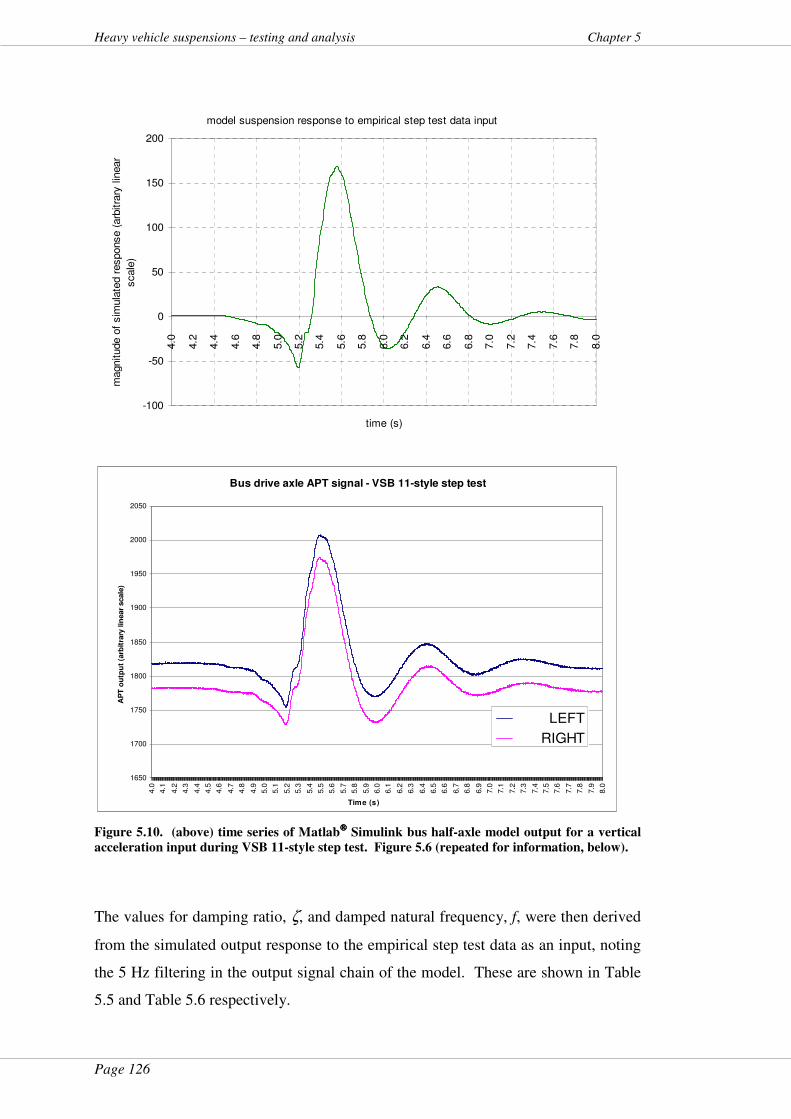
Page 126
Heavy vehicle suspensions – testing and analysis Chapter 5
model suspension response to empirical step test data input
-100
-50
0
50
100
150
200
4.0
4.2
4.4
4.6
4.8
5.0
5.2
5.4
5.6
5.8
6.0
6.2
6.4
6.6
6.8
7.0
7.2
7.4
7.6
7.8
8.0
time (s)
magnitude o
f sim
ula
ted r
esponse (
arb
itra
ry lin
ear
scale
)
Bus drive axle APT signal - VSB 11-style step test
1650
1700
1750
1800
1850
1900
1950
2000
2050
4.0
4.1
4.2
4.3
4.4
4.5
4.6
4.7
4.8
4.9
5.0
5.1
5.2
5.3
5.4
5.5
5.6
5.7
5.8
5.9
6.0
6.1
6.2
6.3
6.4
6.5
6.6
6.7
6.8
6.9
7.0
7.1
7.2
7.3
7.4
7.5
7.6
7.7
7.8
7.9
8.0
Time (s)
AP
T o
utp
ut
(arb
itra
ry lin
ear
scale
)
LEFT
RIGHT
Figure 5.10. (above) time series of Matlab Simulink bus half-axle model output for a vertical
acceleration input during VSB 11-style step test. Figure 5.6 (repeated for information, below).
The values for damping ratio, ζ, and damped natural frequency, f, were then derived
from the simulated output response to the empirical step test data as an input, noting
the 5 Hz filtering in the output signal chain of the model. These are shown in Table
5.5 and Table 5.6 respectively.
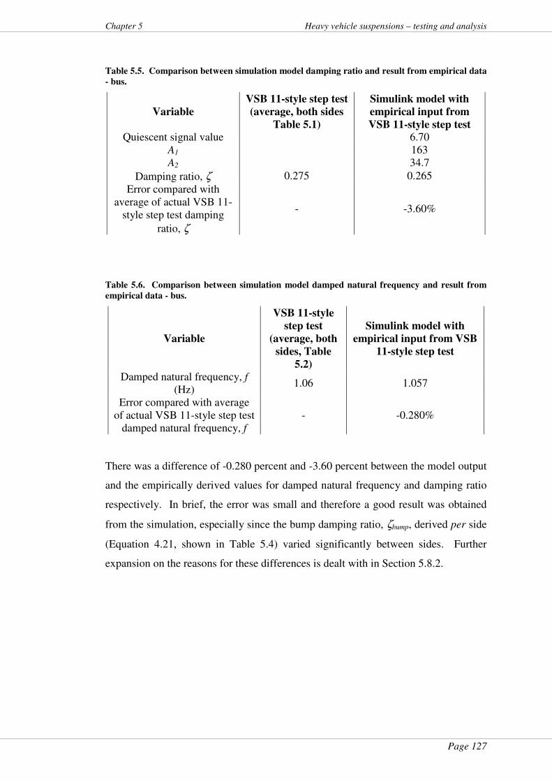
Page 127
Chapter 5 Heavy vehicle suspensions – testing and analysis
Table 5.5. Comparison between simulation model damping ratio and result from empirical data
- bus.
Variable
VSB 11-style step test
(average, both sides
Table 5.1)
Simulink model with
empirical input from
VSB 11-style step test Quiescent signal value 6.70
A1 163 A2 34.7
Damping ratio, ζ 0.275 0.265
Error compared with average of actual VSB 11-
style step test damping
ratio, ζ
- -3.60%
Table 5.6. Comparison between simulation model damped natural frequency and result from
empirical data - bus.
Variable
VSB 11-style
step test
(average, both
sides, Table
5.2)
Simulink model with
empirical input from VSB
11-style step test
Damped natural frequency, f (Hz)
1.06 1.057
Error compared with average of actual VSB 11-style step test
damped natural frequency, f - -0.280%
There was a difference of -0.280 percent and -3.60 percent between the model output
and the empirically derived values for damped natural frequency and damping ratio
respectively. In brief, the error was small and therefore a good result was obtained
from the simulation, especially since the bump damping ratio, ζbump, derived per side
(Equation 4.21, shown in Table 5.4) varied significantly between sides. Further
expansion on the reasons for these differences is dealt with in Section 5.8.2.
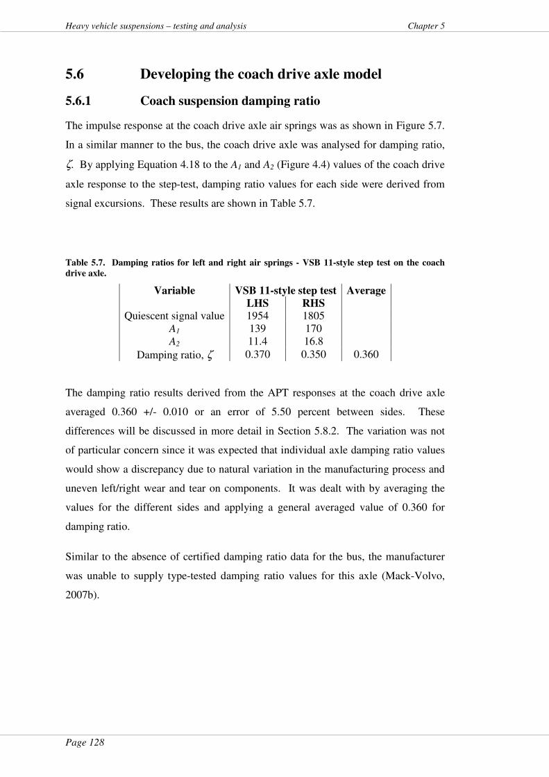
Page 128
Heavy vehicle suspensions – testing and analysis Chapter 5
5.6 Developing the coach drive axle model
5.6.1 Coach suspension damping ratio
The impulse response at the coach drive axle air springs was as shown in Figure 5.7.
In a similar manner to the bus, the coach drive axle was analysed for damping ratio,
ζ. By applying Equation 4.18 to the A1 and A2 (Figure 4.4) values of the coach drive
axle response to the step-test, damping ratio values for each side were derived from
signal excursions. These results are shown in Table 5.7.
Table 5.7. Damping ratios for left and right air springs - VSB 11-style step test on the coach
drive axle.
Variable VSB 11-style step test Average
LHS RHS Quiescent signal value 1954 1805
A1 139 170 A2 11.4 16.8
Damping ratio, ζ 0.370 0.350 0.360
The damping ratio results derived from the APT responses at the coach drive axle
averaged 0.360 +/- 0.010 or an error of 5.50 percent between sides. These
differences will be discussed in more detail in Section 5.8.2. The variation was not
of particular concern since it was expected that individual axle damping ratio values
would show a discrepancy due to natural variation in the manufacturing process and
uneven left/right wear and tear on components. It was dealt with by averaging the
values for the different sides and applying a general averaged value of 0.360 for
damping ratio.
Similar to the absence of certified damping ratio data for the bus, the manufacturer
was unable to supply type-tested damping ratio values for this axle (Mack-Volvo,
2007b).
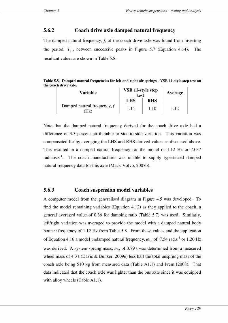
Page 129
Chapter 5 Heavy vehicle suspensions – testing and analysis
5.6.2 Coach drive axle damped natural frequency
The damped natural frequency, f, of the coach drive axle was found from inverting
the period, dT , between successive peaks in Figure 5.7 (Equation 4.14). The
resultant values are shown in Table 5.8.
Table 5.8. Damped natural frequencies for left and right air springs - VSB 11-style step test on
the coach drive axle.
Variable VSB 11-style step
test Average
LHS RHS Damped natural frequency, f
(Hz) 1.14 1.10 1.12
Note that the damped natural frequency derived for the coach drive axle had a
difference of 3.5 percent attributable to side-to-side variation. This variation was
compensated for by averaging the LHS and RHS derived values as discussed above.
This resulted in a damped natural frequency for the model of 1.12 Hz or 7.037
radians.s-1. The coach manufacturer was unable to supply type-tested damped
natural frequency data for this axle (Mack-Volvo, 2007b).
5.6.3 Coach suspension model variables
A computer model from the generalised diagram in Figure 4.5 was developed. To
find the model remaining variables (Equation 4.12) as they applied to the coach, a
general averaged value of 0.36 for damping ratio (Table 5.7) was used. Similarly,
left/right variation was averaged to provide the model with a damped natural body
bounce frequency of 1.12 Hz from Table 5.8. From these values and the application
of Equation 4.16 a model undamped natural frequency, nω , of 7.54 rad.s-1 or 1.20 Hz
was derived. A system sprung mass, ms, of 3.79 t was determined from a measured
wheel mass of 4.3 t (Davis & Bunker, 2009e) less half the total unsprung mass of the
coach axle being 510 kg from measured data (Table A1.1) and Prem (2008). That
data indicated that the coach axle was lighter than the bus axle since it was equipped
with alloy wheels (Table A1.1).
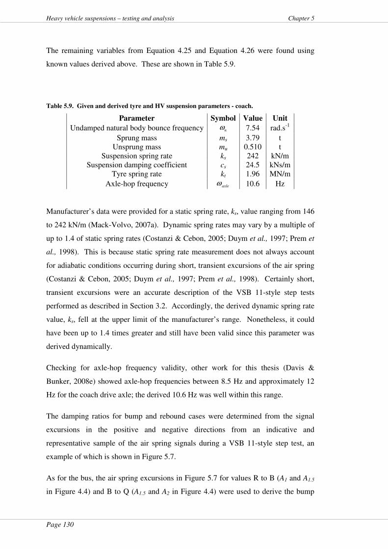
Page 130
Heavy vehicle suspensions – testing and analysis Chapter 5
The remaining variables from Equation 4.25 and Equation 4.26 were found using
known values derived above. These are shown in Table 5.9.
Table 5.9. Given and derived tyre and HV suspension parameters - coach.
Parameter Symbol Value Unit
Undamped natural body bounce frequency nω 7.54 rad.s-1
Sprung mass ms 3.79 t Unsprung mass mu 0.510 t
Suspension spring rate ks 242 kN/m Suspension damping coefficient cs 24.5 kNs/m
Tyre spring rate kt 1.96 MN/m
Axle-hop frequency axleω 10.6 Hz
Manufacturer’s data were provided for a static spring rate, ks, value ranging from 146
to 242 kN/m (Mack-Volvo, 2007a). Dynamic spring rates may vary by a multiple of
up to 1.4 of static spring rates (Costanzi & Cebon, 2005; Duym et al., 1997; Prem et
al., 1998). This is because static spring rate measurement does not always account
for adiabatic conditions occurring during short, transient excursions of the air spring
(Costanzi & Cebon, 2005; Duym et al., 1997; Prem et al., 1998). Certainly short,
transient excursions were an accurate description of the VSB 11-style step tests
performed as described in Section 3.2. Accordingly, the derived dynamic spring rate
value, ks, fell at the upper limit of the manufacturer’s range. Nonetheless, it could
have been up to 1.4 times greater and still have been valid since this parameter was
derived dynamically.
Checking for axle-hop frequency validity, other work for this thesis (Davis &
Bunker, 2008e) showed axle-hop frequencies between 8.5 Hz and approximately 12
Hz for the coach drive axle; the derived 10.6 Hz was well within this range.
The damping ratios for bump and rebound cases were determined from the signal
excursions in the positive and negative directions from an indicative and
representative sample of the air spring signals during a VSB 11-style step test, an
example of which is shown in Figure 5.7.
As for the bus, the air spring excursions in Figure 5.7 for values R to B (A1 and A1.5
in Figure 4.4) and B to Q (A1.5 and A2 in Figure 4.4) were used to derive the bump
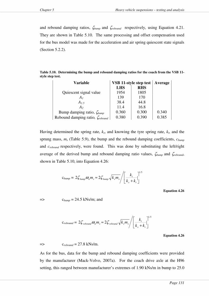
Page 131
Chapter 5 Heavy vehicle suspensions – testing and analysis
and rebound damping ratios, ζbump and ζrebound respectively, using Equation 4.21.
They are shown in Table 5.10. The same processing and offset compensation used
for the bus model was made for the acceleration and air spring quiescent state signals
(Section 5.2.2).
Table 5.10. Determining the bump and rebound damping ratios for the coach from the VSB 11-
style step test.
Variable VSB 11-style step test Average
LHS RHS Quiescent signal value 1954 1805
A1 139 170 A1.5 38.4 44.8 A2 11.4 16.8
Bump damping ratio, ζbump 0.360 0.300 0.340
Rebound damping ratio, ζrebound 0.380 0.390 0.385
Having determined the spring rate, ks, and knowing the tyre spring rate, kt, and the
sprung mass, ms (Table 5.9), the bump and the rebound damping coefficients, cbump
and crebound respectively, were found. This was done by substituting the left/right
average of the derived bump and rebound damping ratio values, ζbump and ζrebound,
shown in Table 5.10, into Equation 4.26:
cbump =
5.1
22
+≈
ts
tssbumpsnbump
kk
kmkm ζωζ
Equation 4.26
=> cbump = 24.5 kNs/m; and
crebound =
5.1
22
+≈
ts
tssreboundsnrebound
kk
kmkm ζωζ
Equation 4.26
=> crebound = 27.8 kNs/m.
As for the bus, data for the bump and rebound damping coefficients were provided
by the manufacturer (Mack-Volvo, 2007a). For the coach drive axle at the H96
setting, this ranged between manufacturer’s extremes of 1.90 kNs/m in bump to 25.0
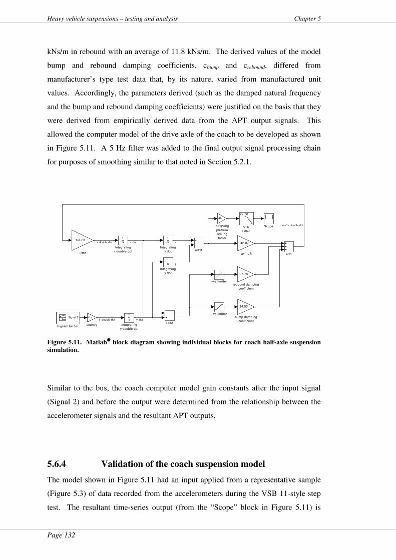
Page 132
Heavy vehicle suspensions – testing and analysis Chapter 5
kNs/m in rebound with an average of 11.8 kNs/m. The derived values of the model
bump and rebound damping coefficients, cbump and crebound, differed from
manufacturer’s type test data that, by its nature, varied from manufactured unit
values. Accordingly, the parameters derived (such as the damped natural frequency
and the bump and rebound damping coefficients) were justified on the basis that they
were derived from empirically derived data from the APT output signals. This
allowed the computer model of the drive axle of the coach to be developed as shown
in Figure 5.11. A 5 Hz filter was added to the final output signal processing chain
for purposes of smoothing similar to that noted in Section 5.2.1.
242.07
spring k
27.78
rebound damping
coefficient
-K-
count/g
24.53
bump damping
coefficient
-K-
air spring
pressure
scaling
factor
add2
add1
add
Signal 2
Signal Builder
Scope
1
s
Integrating
y double dot
1
s
Integrating
y dot
1
s
Integrating
x double dot
1
s
Integrating
x dot
butter
5 Hz
Filter
1/3.79
1/ms
- ve l imiter
+ve l imiter
y double dot
ms*x double dot
y
xx double dot x dot
y dot
Figure 5.11. Matlab
block diagram showing individual blocks for coach half-axle suspension
simulation.
Similar to the bus, the coach computer model gain constants after the input signal
(Signal 2) and before the output were determined from the relationship between the
accelerometer signals and the resultant APT outputs.
5.6.4 Validation of the coach suspension model
The model shown in Figure 5.11 had an input applied from a representative sample
(Figure 5.3) of data recorded from the accelerometers during the VSB 11-style step
test. The resultant time-series output (from the “Scope” block in Figure 5.11) is
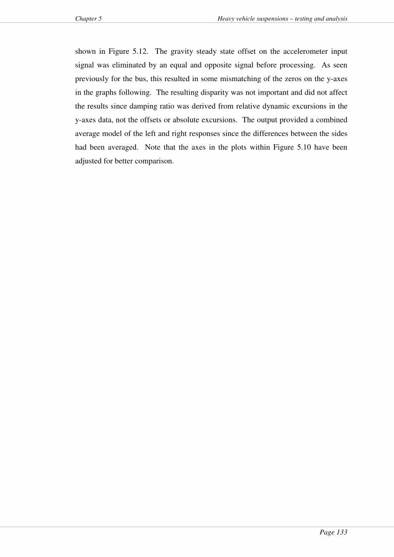
Page 133
Chapter 5 Heavy vehicle suspensions – testing and analysis
shown in Figure 5.12. The gravity steady state offset on the accelerometer input
signal was eliminated by an equal and opposite signal before processing. As seen
previously for the bus, this resulted in some mismatching of the zeros on the y-axes
in the graphs following. The resulting disparity was not important and did not affect
the results since damping ratio was derived from relative dynamic excursions in the
y-axes data, not the offsets or absolute excursions. The output provided a combined
average model of the left and right responses since the differences between the sides
had been averaged. Note that the axes in the plots within Figure 5.10 have been
adjusted for better comparison.
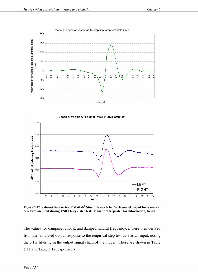
Page 134
Heavy vehicle suspensions – testing and analysis Chapter 5
model suspension response to empirical step test data input
-150
-100
-50
0
50
100
150
200
2.0
2.2
2.4
2.6
2.8
3.0
3.2
3.4
3.6
3.8
4.0
4.2
4.4
4.6
4.8
5.0
5.2
5.4
5.6
5.8
6.0
time (s)
magnitude o
f sim
ula
ted r
esponse (
arb
itra
ry lin
ear
scale
)
Coach drive axle APT signal - VSB 11-style step test
1600
1700
1800
1900
2000
2100
2200
2.0
2.2
2.4
2.6
2.8
3.0
3.2
3.4
3.6
3.8
4.0
4.2
4.4
4.6
4.8
5.0
5.2
5.4
5.6
5.8
6.0
Time (s)
AP
T o
utp
ut (a
rbitra
ry lin
ea
r s
ca
le)
LEFT
RIGHT
Figure 5.12. (above) time series of Matlab Simulink coach half-axle model output for a vertical
acceleration input during VSB 11-style step test. Figure 5.7 (repeated for information) below.
The values for damping ratio, ζ, and damped natural frequency, f, were then derived
from the simulated output response to the empirical step test data as an input, noting
the 5 Hz filtering in the output signal chain of the model. These are shown in Table
5.11 and Table 5.12 respectively.
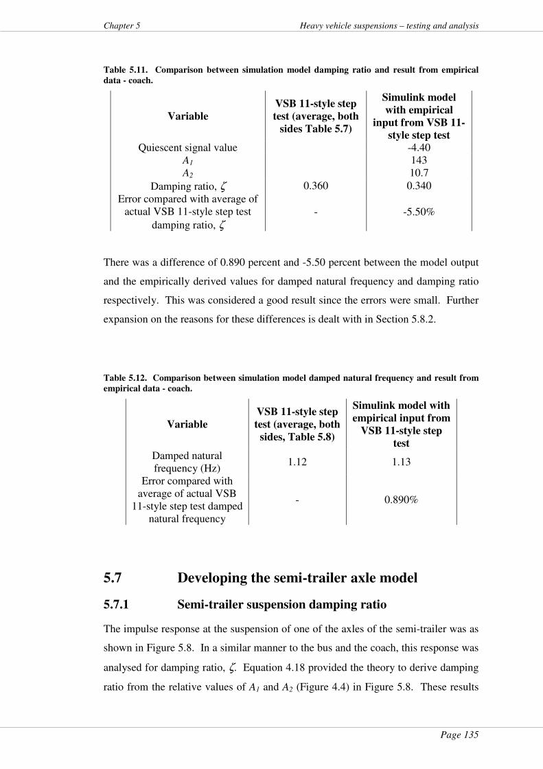
Page 135
Chapter 5 Heavy vehicle suspensions – testing and analysis
Table 5.11. Comparison between simulation model damping ratio and result from empirical
data - coach.
Variable
VSB 11-style step
test (average, both
sides Table 5.7)
Simulink model
with empirical
input from VSB 11-
style step test Quiescent signal value -4.40
A1 143 A2 10.7
Damping ratio, ζ 0.360 0.340
Error compared with average of actual VSB 11-style step test
damping ratio, ζ
- -5.50%
There was a difference of 0.890 percent and -5.50 percent between the model output
and the empirically derived values for damped natural frequency and damping ratio
respectively. This was considered a good result since the errors were small. Further
expansion on the reasons for these differences is dealt with in Section 5.8.2.
Table 5.12. Comparison between simulation model damped natural frequency and result from
empirical data - coach.
Variable
VSB 11-style step
test (average, both
sides, Table 5.8)
Simulink model with
empirical input from
VSB 11-style step
test Damped natural frequency (Hz)
1.12 1.13
Error compared with average of actual VSB
11-style step test damped natural frequency
- 0.890%
5.7 Developing the semi-trailer axle model
5.7.1 Semi-trailer suspension damping ratio
The impulse response at the suspension of one of the axles of the semi-trailer was as
shown in Figure 5.8. In a similar manner to the bus and the coach, this response was
analysed for damping ratio, ζ. Equation 4.18 provided the theory to derive damping
ratio from the relative values of A1 and A2 (Figure 4.4) in Figure 5.8. These results

Page 136
Heavy vehicle suspensions – testing and analysis Chapter 5
are shown in Table 5.13.
Table 5.13. Damping ratios for left and right air springs - VSB 11-style step test on the semi-
trailer axle. Variable VSB 11-style step test Average
LHS RHS Quiescent signal value 1479 1500
A1 94.0 98.0 A2 17.0 21.0
Damping ratio, ζ 0.240 0.260 0.250
Comparing the APT damping ratios per side, it may be noted that the variation in
damping ratio results between sides of the semi-trailer was 0.02 (or a left/right
variation of approximately 8 percent) for an averaged value of 0.25. From a “pull-
up-and-drop” method (Australia Department of Transport and Regional Services,
2004a, 2004c), the manufacturer quoted VSB 11 type-tested damping ratio values for
these axles (Colrain, 2007) of 0.2501. The difference between the derived value and
the manufacturer’s value will be addressed briefly in Section 5.7.3 in preparation for
the detail in Section 5.8.2 which will also address the variation in damping ratios per
side.
5.7.2 Semi-trailer axle damped natural frequency
The damped natural frequency, f, of the semi-trailer axle was found from the inverse
of the time between successive peaks in Figure 5.8 by inverting the damped natural
period ( 1−dT , Equation 4.14), where Td is the damped natural period). The resultant
values for damped natural frequency are shown in Table 5.14.
Table 5.14. Damped natural frequencies for left and right air springs - VSB 11-style step test on
the front axle of the semi-trailer.
Variable VSB 11-style step
test Average
LHS RHS Damped natural frequency f
(Hz) 1.68 1.72 1.70
Page 137
Chapter 5 Heavy vehicle suspensions – testing and analysis
Comparing the two sides in Table 5.14, the damped natural frequency derived for
this axle differed by a maximum of 2.3 percent. To address this difference briefly,
the manufacturer quoted the damped natural frequency for the semi-trailer axle at
1.89 Hz (Colrain, 2007) from a “pull-up-and-drop” VSB 11 type test method with
masses as used during the testing for this thesis. These data are type-test values, as
are all VSB 11 parameters (Davis & Bunker, 2007). Some potential reasons for
differences between these and the tested values were evident. These will be dealt
with briefly in Section 5.7.3 and in detail in Section 5.8.2.
5.7.3 Empirical data and metrics derived thereby vs. VSB 11
type test data
The VSB 11-style test used for the testing in Section 3.2.3 was a step down, without
first pulling up the HV. Individual axle metrics will differ with natural variation in
the manufacturing process as well as other factors mentioned previously such as
mechanical wear and tear. VSB 11 is a type test and type tests do not always reflect
production values. Further, differing HV test methods will produce different results
(Uffelmann & Walter, 1994). That work, for instance, noted differences of up to 60
percent in damping ratio results depending on whether the test was a “lift and drop”,
traverse over a bump or a step down. That dampers have differential rates depending
on direction is a large contributory factor to this phenomenon. Wear and tear in the
HV tested may also have been a factor, even with the precaution of installing new
shock absorbers. More discussion on this issue is contained in Section 5.8.2.
5.7.4 Semi-trailer suspension model variables
A semi-trailer half-axle model was developed from the generalised diagram in Figure
4.5. To find the model remaining variables (Equation 4.12) as they applied to the
axle tested, a general averaged damping ratio value of 0.25 was used from Table
5.13, compensating for the differences in left and right values of damping ratio on
both sides of the semi-trailer axle as discussed briefly above. Similarly, by averaging
the left and right side values for the damped natural frequency for the model, 1.70 Hz
or 10.68 rad.s-1 (Table 5.14). The undamped natural frequency, nω , was then found
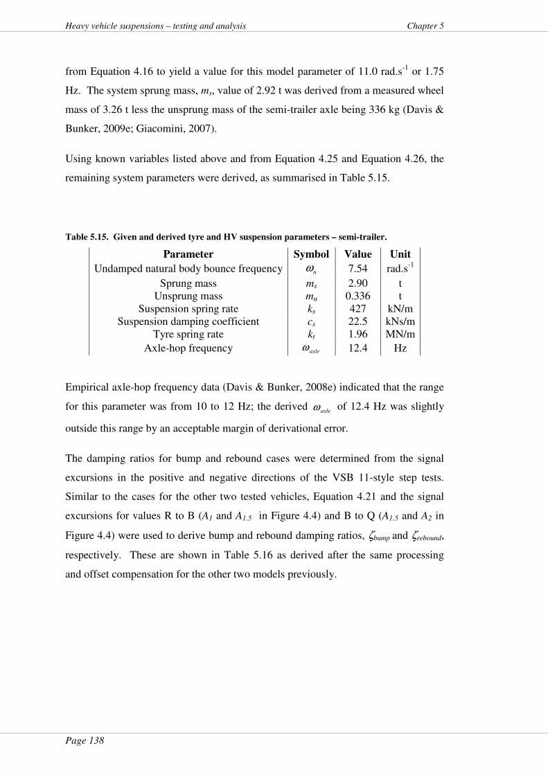
Page 138
Heavy vehicle suspensions – testing and analysis Chapter 5
from Equation 4.16 to yield a value for this model parameter of 11.0 rad.s-1 or 1.75
Hz. The system sprung mass, ms, value of 2.92 t was derived from a measured wheel
mass of 3.26 t less the unsprung mass of the semi-trailer axle being 336 kg (Davis &
Bunker, 2009e; Giacomini, 2007).
Using known variables listed above and from Equation 4.25 and Equation 4.26, the
remaining system parameters were derived, as summarised in Table 5.15.
Table 5.15. Given and derived tyre and HV suspension parameters – semi-trailer.
Parameter Symbol Value Unit
Undamped natural body bounce frequency nω 7.54 rad.s-1
Sprung mass ms 2.90 t Unsprung mass mu 0.336 t
Suspension spring rate ks 427 kN/m Suspension damping coefficient cs 22.5 kNs/m
Tyre spring rate kt 1.96 MN/m
Axle-hop frequency axleω 12.4 Hz
Empirical axle-hop frequency data (Davis & Bunker, 2008e) indicated that the range
for this parameter was from 10 to 12 Hz; the derived axleω of 12.4 Hz was slightly
outside this range by an acceptable margin of derivational error.
The damping ratios for bump and rebound cases were determined from the signal
excursions in the positive and negative directions of the VSB 11-style step tests.
Similar to the cases for the other two tested vehicles, Equation 4.21 and the signal
excursions for values R to B (A1 and A1.5 in Figure 4.4) and B to Q (A1.5 and A2 in
Figure 4.4) were used to derive bump and rebound damping ratios, ζbump and ζrebound,
respectively. These are shown in Table 5.16 as derived after the same processing
and offset compensation for the other two models previously.
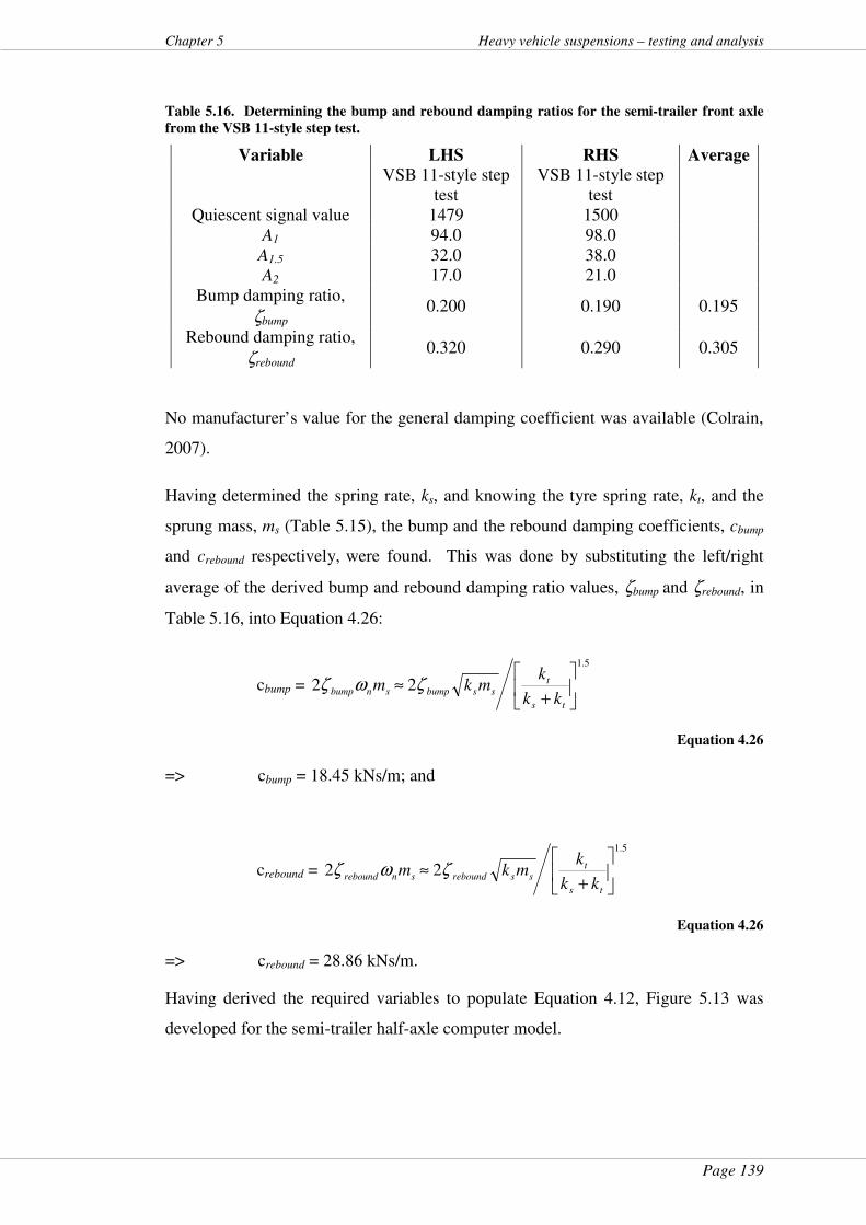
Page 139
Chapter 5 Heavy vehicle suspensions – testing and analysis
Table 5.16. Determining the bump and rebound damping ratios for the semi-trailer front axle
from the VSB 11-style step test.
Variable LHS RHS Average
VSB 11-style step
test VSB 11-style step
test
Quiescent signal value 1479 1500 A1 94.0 98.0 A1.5 32.0 38.0 A2 17.0 21.0
Bump damping ratio,
ζbump
0.200 0.190 0.195
Rebound damping ratio,
ζrebound 0.320 0.290 0.305
No manufacturer’s value for the general damping coefficient was available (Colrain,
2007).
Having determined the spring rate, ks, and knowing the tyre spring rate, kt, and the
sprung mass, ms (Table 5.15), the bump and the rebound damping coefficients, cbump
and crebound respectively, were found. This was done by substituting the left/right
average of the derived bump and rebound damping ratio values, ζbump and ζrebound, in
Table 5.16, into Equation 4.26:
cbump =
5.1
22
+≈
ts
tssbumpsnbump
kk
kmkm ζωζ
Equation 4.26
=> cbump = 18.45 kNs/m; and
crebound =
5.1
22
+≈
ts
tssreboundsnrebound
kk
kmkm ζωζ
Equation 4.26
=> crebound = 28.86 kNs/m.
Having derived the required variables to populate Equation 4.12, Figure 5.13 was
developed for the semi-trailer half-axle computer model.
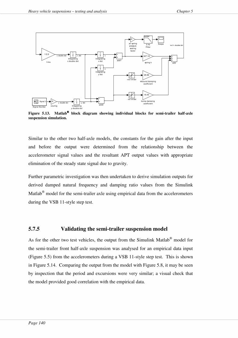
Page 140
Heavy vehicle suspensions – testing and analysis Chapter 5
427.18
spring k
28.86
rebound damping
coefficient
-K-
count/g
18.45
bump damping
coefficient
-K-
air spring
pressure
scaling
factor
add2
add1
add
Signal 2
Signal Builder
Scope
1
s
Integrating
y double dot
1
s
Integrating
y dot
1
s
Integrating
x double dot
1
s
Integrating
x dot
butter
5 Hz
Filter
1/2.9
1/ms
- ve limiter
+ve limiter
y double dot
ms*x double dot
y
xx double dot x dot
y dot
Figure 5.13. Matlab
block diagram showing individual blocks for semi-trailer half-axle
suspension simulation.
Similar to the other two half-axle models, the constants for the gain after the input
and before the output were determined from the relationship between the
accelerometer signal values and the resultant APT output values with appropriate
elimination of the steady state signal due to gravity.
Further parametric investigation was then undertaken to derive simulation outputs for
derived damped natural frequency and damping ratio values from the Simulink
Matlab model for the semi-trailer axle using empirical data from the accelerometers
during the VSB 11-style step test.
5.7.5 Validating the semi-trailer suspension model
As for the other two test vehicles, the output from the Simulink Matlab model for
the semi-trailer front half-axle suspension was analysed for an empirical data input
(Figure 5.5) from the accelerometers during a VSB 11-style step test. This is shown
in Figure 5.14. Comparing the output from the model with Figure 5.8, it may be seen
by inspection that the period and excursions were very similar; a visual check that
the model provided good correlation with the empirical data.

Page 141
Chapter 5 Heavy vehicle suspensions – testing and analysis
model suspension response to empirical step test data input
-100
-50
0
50
100
150
4.0
4.2
4.4
4.6
4.8
5.0
5.2
5.4
5.6
5.8
6.0
6.2
6.4
6.6
6.8
7.0
7.2
7.4
7.6
7.8
8.0
time (s)
magnitude o
f sim
ula
ted r
esponse (
arb
itra
ry lin
ear
scale
)
Semi-trailer front APT signal - VSB 11-style setp test
1250
1300
1350
1400
1450
1500
1550
1600
1650
3.9
4.1
4.3
4.5
4.7
4.9
5.1
5.3
5.5
5.7
5.9
6.1
6.3
6.5
6.7
6.9
7.1
7.3
7.5
7.7
7.9
Time (s)
AP
T o
utp
ut
- a
rbit
rary
lin
ea
r s
ac
le
LEFT
RIGHT
Figure 5.14. (above) time series of Matlab Simulink semi-trailer half-axle model output for a
vertical acceleration input during VSB 11-style step test. Figure 5.8 (repeated for information)
below.
The model’s values for damping ratio and damped natural frequency were then
derived for this input. These are shown in Table 5.17 and Table 5.18 respectively,
after 5 Hz filtering.

Page 142
Heavy vehicle suspensions – testing and analysis Chapter 5
Table 5.17. Comparison between simulation model damping ratio and result from empirical
data – semi-trailer.
Variable
VSB 11-style step test
(average, both sides
Table 5.7)
Simulink model with
empirical input from
VSB 11-style step test Quiescent signal value 2.50
A1 104 A2 21.8
Damping ratio, ζ 0.250 0.240
Error compared with average of actual VSB
11-style step test damping ratio
- -4.00%
There was a difference of -4.00 percent between the model output and the
empirically derived values for damping ratio. Expansion on possible reasons for this
result is contained in Section 5.8.2.
Table 5.18. Comparison between simulation model damped natural frequency and result from
empirical data – semi-trailer.
Variable
VSB 11-style step
test (average, both
sides, Table 5.8)
Simulink model with
empirical input from
VSB 11-style step test Damped natural frequency
(Hz) 1.70 1.65
Error compared with average of actual VSB 11-
style step test damped natural frequency, f
- -2.90%
There was a difference of -2.90 percent between the model output and the
empirically derived values for damped natural frequency. The variation between
sides of these parameters for the VSB 11-style step tests (Table 5.13 and Table 5.14)
was 8.3 percent and 2.3 percent respectively.
Comparing the left/right variation of suspension parameters derived empirically
using the “gold standard” test procedure, the errors between the model output and the
actual data were of the same order-of-magnitude. This was considered a satisfactory
result with respect to generally-accepted experimental error. Further expansion on
the reasons for any differences is dealt with in Section 5.8.2.
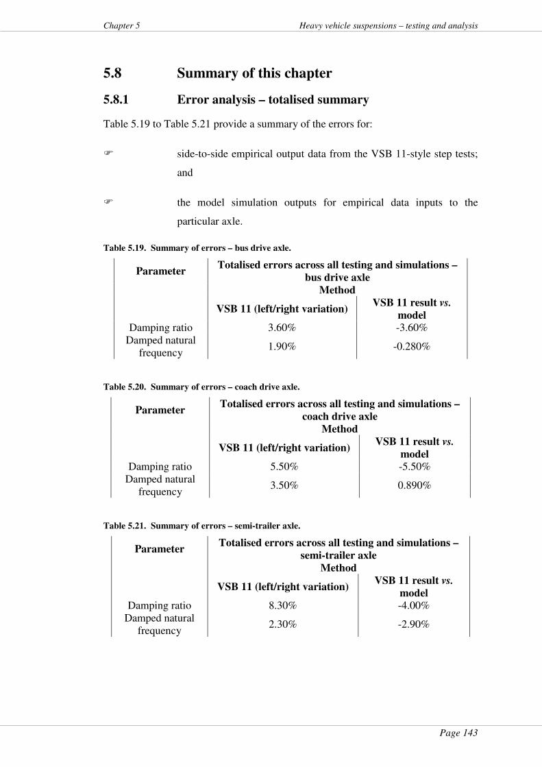
Page 143
Chapter 5 Heavy vehicle suspensions – testing and analysis
5.8 Summary of this chapter
5.8.1 Error analysis – totalised summary
Table 5.19 to Table 5.21 provide a summary of the errors for:
� side-to-side empirical output data from the VSB 11-style step tests;
and
� the model simulation outputs for empirical data inputs to the
particular axle.
Table 5.19. Summary of errors – bus drive axle.
Parameter Totalised errors across all testing and simulations –
bus drive axle
Method
VSB 11 (left/right variation) VSB 11 result vs.
model Damping ratio 3.60% -3.60%
Damped natural frequency
1.90% -0.280%
Table 5.20. Summary of errors – coach drive axle.
Parameter Totalised errors across all testing and simulations –
coach drive axle
Method
VSB 11 (left/right variation) VSB 11 result vs.
model Damping ratio 5.50% -5.50%
Damped natural frequency
3.50% 0.890%
Table 5.21. Summary of errors – semi-trailer axle.
Parameter Totalised errors across all testing and simulations –
semi-trailer axle
Method
VSB 11 (left/right variation) VSB 11 result vs.
model Damping ratio 8.30% -4.00%
Damped natural frequency
2.30% -2.90%
Page 144
Heavy vehicle suspensions – testing and analysis Chapter 5
5.8.2 Regarding the left/right differences from empirical
data, VSB 11 data and also the model outputs
The errors shown in Table 5.19 to Table 5.21 may be considered in light of the
following discussion. Manufacturer’s data for the semi-trailer were supplied for
damped natural frequency and damping ratio. These data were for VSB 11 type-
tested values (Davis & Bunker, 2007). Differences between these and the tested
values from this project were evident. As with all manufacturing process, there will
be natural variation in any system that will cause data from one individual unit to
vary from the type-tested metrics. This will also be the case for differences between
type tested damping coefficients and those derived empirically herein for the bus and
the coach.
Even though the dampers were renewed for all the HVs tested, other suspension
components would undoubtedly have undergone mechanical wear and tear compared
with their new state. Notably, where supplied, the coach and bus manufacturer’s
parametric data did not differ per side. Accordingly, any variations in the
empirically derived data per side were due to uneven wear and tear, manufacturing
tolerances and measurement error. This last should have been evenly divided
between sides and was minimal, as shown in other work (Davis, 2006b; Karl et al.,
2009b) and in Appendix 2. Potholes predominate on the left hand side of the road in
Australia and instantaneous axle forces as derived later in this thesis were higher on
the left compared with the right hand side (Davis & Bunker, 2009a). It is not
surprising to expect that such wear and tear would have been greater on the left
therefore, causing an imbalance in both suspension component wear and also more
frequent component replacement on that side. Further, differences of up to 60
percent in damping ratio values have been reported (Uffelmann & Walter, 1994)
depending on direction of excitation. As noted in Table 5.4, Table 5.10 and Table
5.16 as well as from the manufacturer (Mack-Volvo, 2007a), dampers have
differential rates depending on direction. The directionality of damper response is an
important contributory factor to the phenomenon of different results, dependent on
different test methods. That is, some test methods drop the HV axle, exercising one
direction before the other. Other methods lift and drop, reversing the order of the
halves on the excitation impulse (Uffelmann & Walter, 1994).
Page 145
Chapter 5 Heavy vehicle suspensions – testing and analysis
The models developed were not particularly complex compared with some others
such as those of Costanzi and Cebon (2005, 2006). There were, however, of similar
complexity to other work (Cole & Cebon, 2007; Duym et al., 1997; Prem et al.,
1998). The model parameters were composites derived from averaged empirical left
and right hand side data from the vehicles tested. This resulted in the model outputs
being composites of the left and right averages of all the model parameters and their
inputs. Nonetheless, the computer models produced damped natural frequency and
damping ratio values very close to the empirical results. Further, should the
differences in parameters between sides derived by the use of the VSB 11-style step
test inform likely error margins, the errors between the model outputs compared with
the empirical data were of the same order of magnitude.
VSB 11 (Australia Department of Transport and Regional Services, 2004c) is the
Australian “gold standard” for parametric measurement of “road friendly” HV
suspensions. There was only one set of available VSB 11-derived suspension data
for the HVs tested as described in Section 3.2; that for the semi-trailer axles.
Empirical data from the VSB 11-style step test in Section 3.2 were used as an input
to the semi-trailer model. The difference between the damping ratio from that
model’s output, the VSB 11-certified damping ratio and the VSB 11-style step test
damping ratio result was 0.01 (Table 5.17). This was an error of -4.0 percent. As
noted in Section 5.7.3, variations of up to 60 percent have been reported between
results from different types of impulse testing (Prem et al., 1998; Uffelmann &
Walter, 1994). Similarly, the difference between the VSB 11-certified damped
natural frequency and the semi-trailer model damped natural frequency was -2.9%.
All the model output errors were within, or less than, the same order-of-magnitude of
left/right variation apparent from the empirical data recorded during the step test
defined in VSB 11. This result, combined with the potential for variation in data due
to different excitation methods, was considered a satisfactory outcome with respect
to generally-accepted experimental error.
Page 146
Heavy vehicle suspensions – testing and analysis Chapter 5
5.9 Conclusions from this chapter
5.9.1 General
The maximum time of impulse duration recommended by Doebelin (1980) for
characterising a system is 0.35/f where f is the damped natural frequency (Equation
4.14). Therefore, to characterise the bus and coach suspension systems, the impulse
duration would, taking their damped natural frequencies from Table 5.2 and Table
5.8, ideally have been:
s33.0 to31.01
35.0 ≈×f
and the semi-trailer impulse duration with a damped natural frequency of 1.7 Hz
(Table 5.14) would ideally have been:
s18.01
35.0 ≈×f
The VSB 11-style step test input impulse durations were all approximately 0.4 s
(Figure 5.3 to Figure 5.5); slightly longer than Doebelin’s recommendation. This
slight increase in duration may have contributed to the small variations in the
measured values for damped natural frequency as predicted by Doebelin, pp. 79 - 81
(1980). Nonetheless, the model outputs showed good correlation with empirical
output data for the same input data.
5.10 Chapter close
Chapter 3, Section 3.2 described methodology for a novel, low cost HV suspension
test, the “pipe test” where a HV wheel was rolled over a 50 mm steel pipe at low
speed with the air spring response measured. The models developed in this chapter,
now validated against empirical data for damped natural frequency and damping
ratio, will be used to determine the validity of that low cost test method in Chapter 6.
Further, Chapter 12, Section 12.2.4 will explore the results of using three of the
semi-trailer axle models (Figure 5.13) developed in this chapter formed into a tri-axle
group. This meta-model will be used to explore the ability of a simulated semi-
Page 147
Chapter 5 Heavy vehicle suspensions – testing and analysis
trailer group to distribute load at the air springs for varying levels of air line
connectivity between axles. Accordingly, the models developed and validated in this
Chapter will allow exploration of the theoretical limits of air spring suspension load
sharing in Chapter 12.
Links where this chapter informs other chapters of this thesis are shown in Figure
1.4.
“Let not the perfect be the enemy of the good.” - Voltaire (attrib.)
Page 148
Heavy vehicle suspensions – testing and analysis Chapter 6
6 Quasi-static suspension testing and
parametric model outputs
6.1 About this chapter
This chapter presents analysis of the data gathered as described in Section 3.2.3. In
it, “pipe test” data are compared with the VSB 11-style step test results. Simulation
models were developed in Chapter 4 and validated in Chapter 5. These simulation
models were used in an exercise where empirical “pipe test” data were used as inputs
to those models. Correlation of the results of that exercise with the results from VSB
11-style testing in Section 3.2.3 is detailed.
6.2 Introduction
As detailed in Chapter 1, a low cost suspension test needed to be developed to meet
Objective 3 of this project. The quasi-static testing detailed in Section 3.2.3 for the
“pipe test” vs. the VSB 11-style test was analysed to compare the VSB 11-style step
test results with the results from the low-cost “pipe test”.
Due to scheduling and logistical constraints of the overall test programme, only one
“pipe test” was conducted per test heavy vehicle (HV). Accordingly, the results and
analysis of the “pipe test” in this chapter are detailed as a “proof-of-concept” rather
than a full implementation approach to that test within a statistically significant
developmental framework.
The coach and the semi-trailer “pipe tests” did not yield signals analysable for
damping ratio. Nonetheless, acceleration data from the bus “pipe test” were used as
an input to the three HV models developed and validated in Chapter 5. This was to
broaden the scope of the project to more than just the one successful “pipe test”. The
output data from these simulations, as an analogue of air spring pressure, were then
compared with the derived values for the suspensions tested using the VSB 11-style
step tests. The results of those comparisons are detailed and analysed in this chapter.
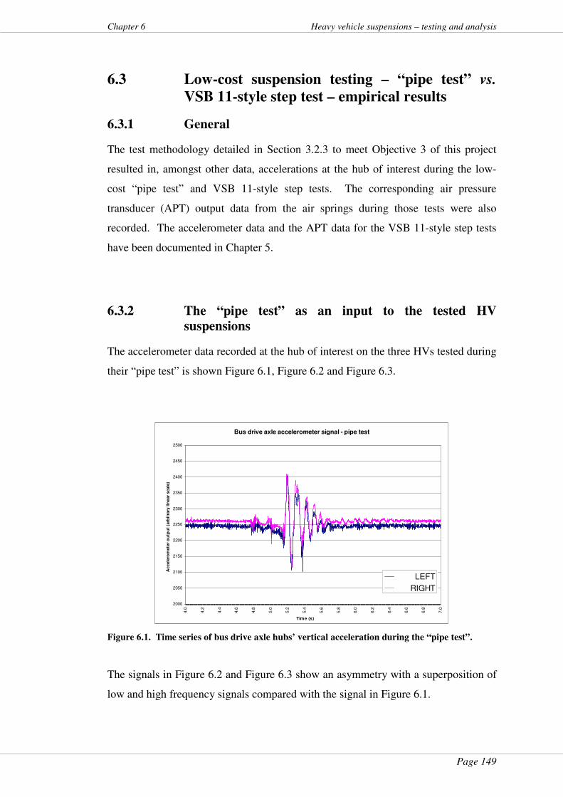
Page 149
Chapter 6 Heavy vehicle suspensions – testing and analysis
6.3 Low-cost suspension testing – “pipe test” vs.
VSB 11-style step test – empirical results
6.3.1 General
The test methodology detailed in Section 3.2.3 to meet Objective 3 of this project
resulted in, amongst other data, accelerations at the hub of interest during the low-
cost “pipe test” and VSB 11-style step tests. The corresponding air pressure
transducer (APT) output data from the air springs during those tests were also
recorded. The accelerometer data and the APT data for the VSB 11-style step tests
have been documented in Chapter 5.
6.3.2 The “pipe test” as an input to the tested HV
suspensions
The accelerometer data recorded at the hub of interest on the three HVs tested during
their “pipe test” is shown Figure 6.1, Figure 6.2 and Figure 6.3.
Bus drive axle accelerometer signal - pipe test
2000
2050
2100
2150
2200
2250
2300
2350
2400
2450
2500
4.0
4.2
4.4
4.6
4.8
5.0
5.2
5.4
5.6
5.8
6.0
6.2
6.4
6.6
6.8
7.0
Time (s)
Accele
rom
ete
r o
utp
ut
(arb
itra
ry lin
ear
scale
)
LEFT
RIGHT
Figure 6.1. Time series of bus drive axle hubs’ vertical acceleration during the “pipe test”.
The signals in Figure 6.2 and Figure 6.3 show an asymmetry with a superposition of
low and high frequency signals compared with the signal in Figure 6.1.
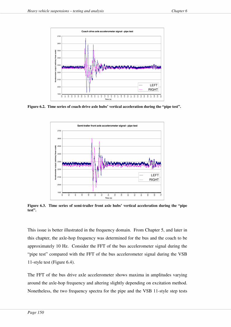
Page 150
Heavy vehicle suspensions – testing and analysis Chapter 6
Coach drive axle accelerometer signal - pipe test
1900
2000
2100
2200
2300
2400
2500
2600
2700
3.0
3.1
3.2
3.3
3.4
3.5
3.6
3.7
3.8
3.9
4.0
4.1
4.2
4.3
4.4
4.5
4.6
4.7
4.8
4.9
5.0
5.1
5.2
5.3
5.4
5.5
5.6
5.7
5.8
5.9
6.0
Time (s)
Accele
rom
ete
r o
utp
ut
(arb
itra
ry lin
ear
scale
)
LEFT
RIGHT
Figure 6.2. Time series of coach drive axle hubs’ vertical acceleration during the “pipe test”.
Semi-trailer front axle accelerometer signal - pipe test
1900
2000
2100
2200
2300
2400
2500
2600
2700
4.0
4.2
4.4
4.6
4.8
5.0
5.2
5.4
5.6
5.8
6.0
6.2
6.4
6.6
6.8
7.0
Time (s)
Ac
cele
rom
ete
r o
utp
ut
(arb
itra
ry lin
ear
sca
le)
LEFT
RIGHT
Figure 6.3. Time series of semi-trailer front axle hubs’ vertical acceleration during the “pipe
test”.
This issue is better illustrated in the frequency domain. From Chapter 5, and later in
this chapter, the axle-hop frequency was determined for the bus and the coach to be
approximately 10 Hz. Consider the FFT of the bus accelerometer signal during the
“pipe test” compared with the FFT of the bus accelerometer signal during the VSB
11-style test (Figure 6.4).
The FFT of the bus drive axle accelerometer shows maxima in amplitudes varying
around the axle-hop frequency and altering slightly depending on excitation method.
Nonetheless, the two frequency spectra for the pipe and the VSB 11-style step tests
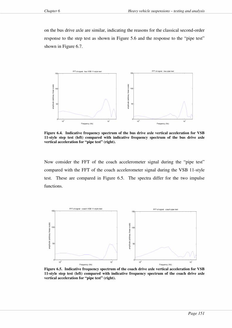
Page 151
Chapter 6 Heavy vehicle suspensions – testing and analysis
on the bus drive axle are similar, indicating the reasons for the classical second-order
response to the step test as shown in Figure 5.6 and the response to the “pipe test”
shown in Figure 6.7.
100
101
0
50
100
150FFT of signal - bus VSB 11-style test
Frequency (Hz)
am
plit
ude (
arb
itra
ry lin
ear
scale
)
100
101
0
50
100
150FFT of signal - bus pipe test
Frequency (Hz)
am
plitu
de (
arb
itra
ry lin
ear
scale
)
Figure 6.4. Indicative frequency spectrum of the bus drive axle vertical acceleration for VSB
11-style step test (left) compared with indicative frequency spectrum of the bus drive axle
vertical acceleration for “pipe test” (right).
Now consider the FFT of the coach accelerometer signal during the “pipe test”
compared with the FFT of the coach accelerometer signal during the VSB 11-style
test. These are compared in Figure 6.5. The spectra differ for the two impulse
functions.
100
101
0
50
100
150FFT of signal - coach VSB 11-style test
Frequency (Hz)
am
plit
ude (
arb
itra
ry lin
ear
scale
)
100
101
0
50
100
150FFT of signal - coach pipe test
Frequency (Hz)
am
plit
ude (
arb
itra
ry lin
ear
scale
)
Figure 6.5. Indicative frequency spectrum of the coach drive axle vertical acceleration for VSB
11-style step test (left) compared with indicative frequency spectrum of the coach drive axle
vertical acceleration for “pipe test” (right).
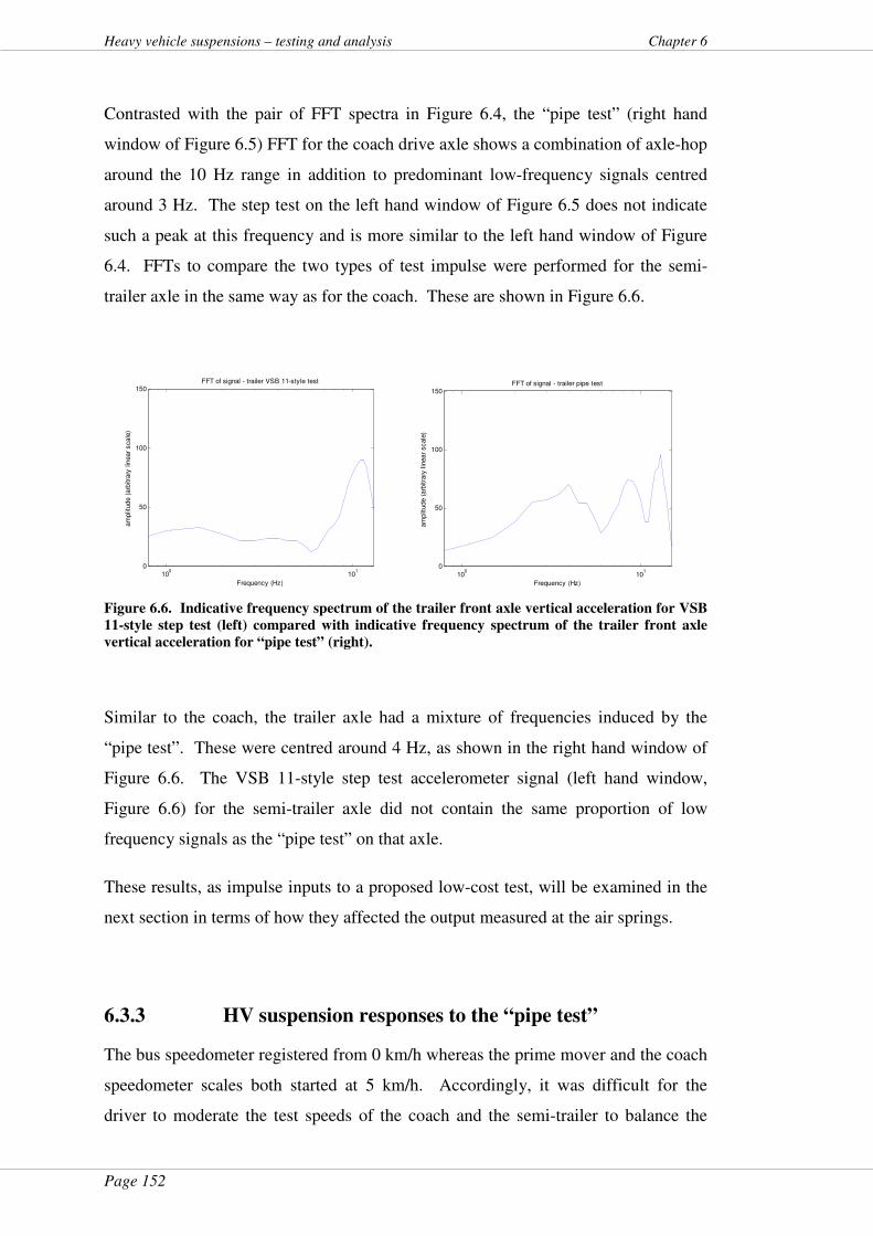
Page 152
Heavy vehicle suspensions – testing and analysis Chapter 6
Contrasted with the pair of FFT spectra in Figure 6.4, the “pipe test” (right hand
window of Figure 6.5) FFT for the coach drive axle shows a combination of axle-hop
around the 10 Hz range in addition to predominant low-frequency signals centred
around 3 Hz. The step test on the left hand window of Figure 6.5 does not indicate
such a peak at this frequency and is more similar to the left hand window of Figure
6.4. FFTs to compare the two types of test impulse were performed for the semi-
trailer axle in the same way as for the coach. These are shown in Figure 6.6.
100
101
0
50
100
150FFT of signal - trailer VSB 11-style test
Frequency (Hz)
am
plit
ude (
arb
itra
ry lin
ear
scale
)
10
010
10
50
100
150FFT of signal - trailer pipe test
Frequency (Hz)
am
plit
ude (
arb
itra
ry lin
ear
scale
)
Figure 6.6. Indicative frequency spectrum of the trailer front axle vertical acceleration for VSB
11-style step test (left) compared with indicative frequency spectrum of the trailer front axle
vertical acceleration for “pipe test” (right).
Similar to the coach, the trailer axle had a mixture of frequencies induced by the
“pipe test”. These were centred around 4 Hz, as shown in the right hand window of
Figure 6.6. The VSB 11-style step test accelerometer signal (left hand window,
Figure 6.6) for the semi-trailer axle did not contain the same proportion of low
frequency signals as the “pipe test” on that axle.
These results, as impulse inputs to a proposed low-cost test, will be examined in the
next section in terms of how they affected the output measured at the air springs.
6.3.3 HV suspension responses to the “pipe test”
The bus speedometer registered from 0 km/h whereas the prime mover and the coach
speedometer scales both started at 5 km/h. Accordingly, it was difficult for the
driver to moderate the test speeds of the coach and the semi-trailer to balance the
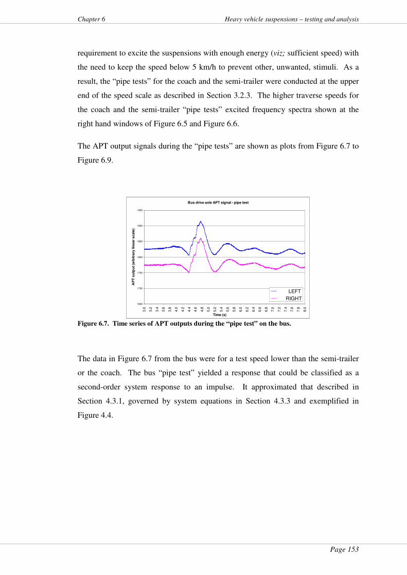
Page 153
Chapter 6 Heavy vehicle suspensions – testing and analysis
requirement to excite the suspensions with enough energy (viz; sufficient speed) with
the need to keep the speed below 5 km/h to prevent other, unwanted, stimuli. As a
result, the “pipe tests” for the coach and the semi-trailer were conducted at the upper
end of the speed scale as described in Section 3.2.3. The higher traverse speeds for
the coach and the semi-trailer “pipe tests” excited frequency spectra shown at the
right hand windows of Figure 6.5 and Figure 6.6.
The APT output signals during the “pipe tests” are shown as plots from Figure 6.7 to
Figure 6.9.
Bus drive axle APT signal - pipe test
1650
1700
1750
1800
1850
1900
1950
3.0
3.2
3.4
3.6
3.8
4.0
4.2
4.4
4.6
4.8
5.0
5.2
5.4
5.6
5.8
6.0
6.2
6.4
6.6
6.8
7.0
7.2
7.4
7.6
7.8
8.0
Time (s)
AP
T o
utp
ut (a
rbitra
ry lin
ear
sca
le)
LEFT
RIGHT
Figure 6.7. Time series of APT outputs during the “pipe test” on the bus.
The data in Figure 6.7 from the bus were for a test speed lower than the semi-trailer
or the coach. The bus “pipe test” yielded a response that could be classified as a
second-order system response to an impulse. It approximated that described in
Section 4.3.1, governed by system equations in Section 4.3.3 and exemplified in
Figure 4.4.

Page 154
Heavy vehicle suspensions – testing and analysis Chapter 6
Coach drive axle APT signal - pipe test
1700
1750
1800
1850
1900
1950
2000
2050
1.0
1.2
1.4
1.6
1.8
2.0
2.2
2.4
2.6
2.8
3.0
3.2
3.4
3.6
3.8
4.0
4.2
4.4
4.6
4.8
5.0
5.2
5.4
5.6
5.8
6.0
6.2
6.4
6.6
6.8
7.0
7.2
7.4
7.6
7.8
8.0
Time (s)
AP
T o
utp
ut
(arb
itra
ry l
inea
r sc
ale
)
LEFT
RIGHT
Figure 6.8. Time series of APT outputs from the coach drive axle during the “pipe test”.
Figure 6.8 and Figure 6.9 show APT output data that were not analysable as second-
order underdamped systems owing to their responses not aligning with those
expected for classical second-order system responses as referenced previously. This
point especially so for damping ratio analysis since the responses did not decay
exponentially as would be expected for a second-order system (Section 4.3.1, 4.3.3
and Figure 4.4).
Semi-trailer front axle APT signal - pipe test
1350
1400
1450
1500
1550
1600
1650
4.0
4.2
4.4
4.6
4.8
5.0
5.2
5.4
5.6
5.8
6.0
6.2
6.4
6.6
6.8
7.0
7.2
7.4
7.6
7.8
8.0
Time (s)
Acce
lero
mete
r o
utp
ut
(arb
itra
ry l
inea
r sca
le)
LEFT
RIGHT
Figure 6.9. Time series of APT outputs from the front semi-trailer axle during the “pipe test”.
Consider the “pipe test” result (Figure 6.7) as a classical second-order system
response, as modelled in Figure 4.4, compared with those for the non-classical
second-order system responses shown in Figure 6.8 and Figure 6.9. For the cases of
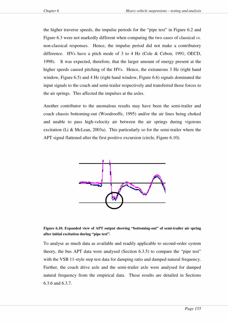
Page 155
Chapter 6 Heavy vehicle suspensions – testing and analysis
the higher traverse speeds, the impulse periods for the “pipe test” in Figure 6.2 and
Figure 6.3 were not markedly different when comparing the two cases of classical vs.
non-classical responses. Hence, the impulse period did not make a contributory
difference. HVs have a pitch mode of 3 to 4 Hz (Cole & Cebon, 1991; OECD,
1998). It was expected, therefore, that the larger amount of energy present at the
higher speeds caused pitching of the HVs. Hence, the extraneous 3 Hz (right hand
window, Figure 6.5) and 4 Hz (right hand window, Figure 6.6) signals dominated the
input signals to the coach and semi-trailer respectively and transferred those forces to
the air springs. This affected the impulses at the axles.
Another contributor to the anomalous results may have been the semi-trailer and
coach chassis bottoming-out (Woodrooffe, 1995) and/or the air lines being choked
and unable to pass high-velocity air between the air springs during vigorous
excitation (Li & McLean, 2003a). This particularly so for the semi-trailer where the
APT signal flattened after the first positive excursion (circle, Figure 6.10).
Figure 6.10. Expanded view of APT output showing “bottoming-out” of semi-trailer air spring
after initial excitation during “pipe test”.
To analyse as much data as available and readily applicable to second-order system
theory, the bus APT data were analysed (Section 6.3.5) to compare the “pipe test”
with the VSB 11-style step test data for damping ratio and damped natural frequency.
Further, the coach drive axle and the semi-trailer axle were analysed for damped
natural frequency from the empirical data. These results are detailed in Sections
6.3.6 and 6.3.7.
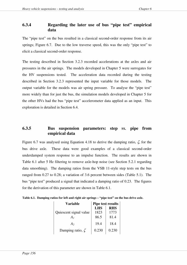
Page 156
Heavy vehicle suspensions – testing and analysis Chapter 6
6.3.4 Regarding the later use of bus “pipe test” empirical
data
The “pipe test” on the bus resulted in a classical second-order response from its air
springs; Figure 6.7. Due to the low traverse speed, this was the only “pipe test” to
elicit a classical second-order response.
The testing described in Section 3.2.3 recorded accelerations at the axles and air
pressures in the air springs. The models developed in Chapter 5 were surrogates for
the HV suspensions tested. The acceleration data recorded during the testing
described in Section 3.2.3 represented the input variable for those models. The
output variable for the models was air spring pressure. To analyse the “pipe test”
more widely than for just the bus, the simulation models developed in Chapter 5 for
the other HVs had the bus “pipe test” accelerometer data applied as an input. This
exploration is detailed in Section 6.4.
6.3.5 Bus suspension parameters: step vs. pipe from
empirical data
Figure 6.7 was analysed using Equation 4.18 to derive the damping ratio, ζ, for the
bus drive axle. These data were good examples of a classical second-order
underdamped system response to an impulse function. The results are shown in
Table 6.1 after 5 Hz filtering to remove axle-hop noise (see Section 5.2.1 regarding
data smoothing). The damping ratios from the VSB 11-style step tests on the bus
ranged from 0.27 to 0.28; a variation of 3.6 percent between sides (Table 5.1). The
bus “pipe test” produced a signal that indicated a damping ratio of 0.23. The figures
for the derivation of this parameter are shown in Table 6.1.
Table 6.1. Damping ratios for left and right air springs – “pipe test” on the bus drive axle.
Variable Pipe test results LHS RHS
Quiescent signal value 1823 1773
A1 86.5 81.4
A2 19.4 18.4
Damping ratio, ζ
0.230 0.230
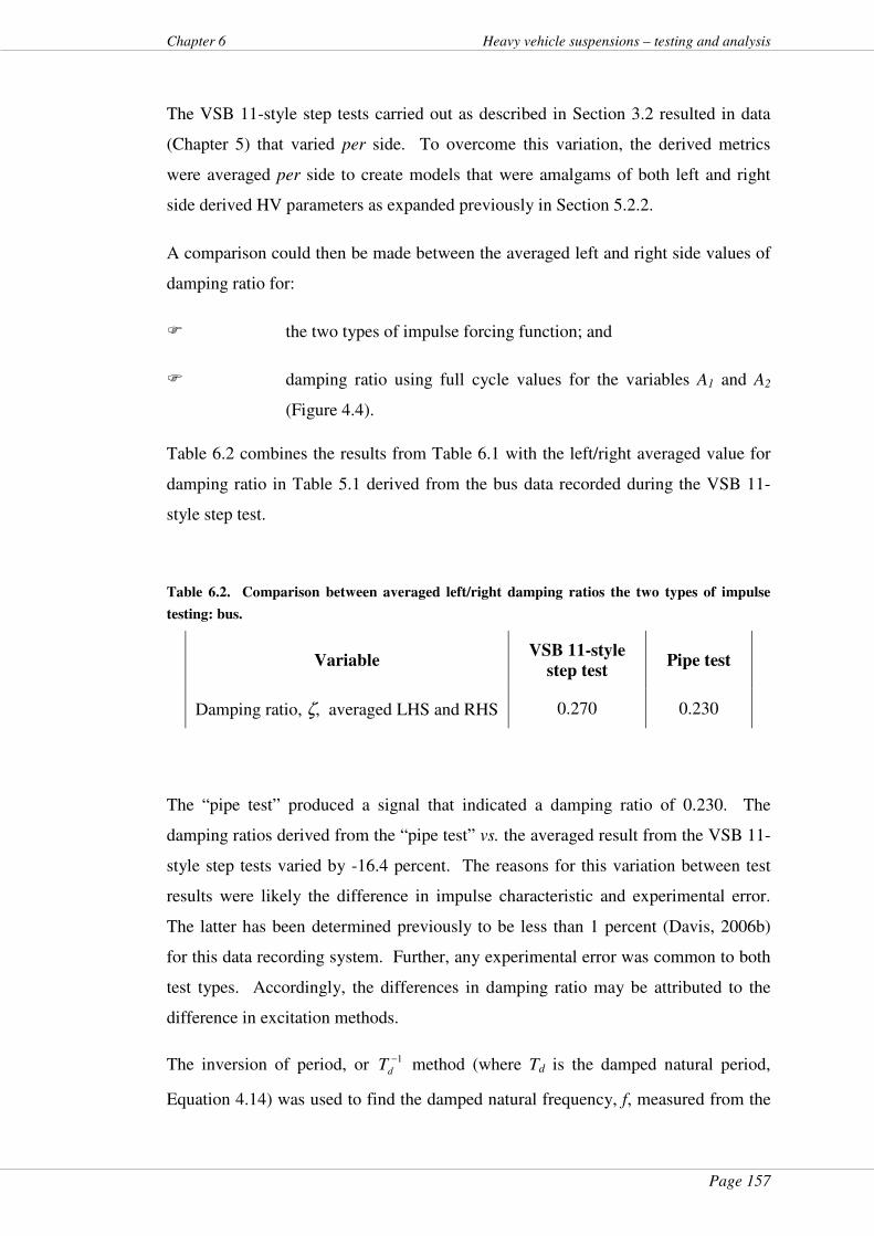
Page 157
Chapter 6 Heavy vehicle suspensions – testing and analysis
The VSB 11-style step tests carried out as described in Section 3.2 resulted in data
(Chapter 5) that varied per side. To overcome this variation, the derived metrics
were averaged per side to create models that were amalgams of both left and right
side derived HV parameters as expanded previously in Section 5.2.2.
A comparison could then be made between the averaged left and right side values of
damping ratio for:
� the two types of impulse forcing function; and
� damping ratio using full cycle values for the variables A1 and A2
(Figure 4.4).
Table 6.2 combines the results from Table 6.1 with the left/right averaged value for
damping ratio in Table 5.1 derived from the bus data recorded during the VSB 11-
style step test.
Table 6.2. Comparison between averaged left/right damping ratios the two types of impulse
testing: bus.
Variable VSB 11-style
step test Pipe test
Damping ratio, ζ, averaged LHS and RHS 0.270 0.230
The “pipe test” produced a signal that indicated a damping ratio of 0.230. The
damping ratios derived from the “pipe test” vs. the averaged result from the VSB 11-
style step tests varied by -16.4 percent. The reasons for this variation between test
results were likely the difference in impulse characteristic and experimental error.
The latter has been determined previously to be less than 1 percent (Davis, 2006b)
for this data recording system. Further, any experimental error was common to both
test types. Accordingly, the differences in damping ratio may be attributed to the
difference in excitation methods.
The inversion of period, or 1−dT method (where Td is the damped natural period,
Equation 4.14) was used to find the damped natural frequency, f, measured from the
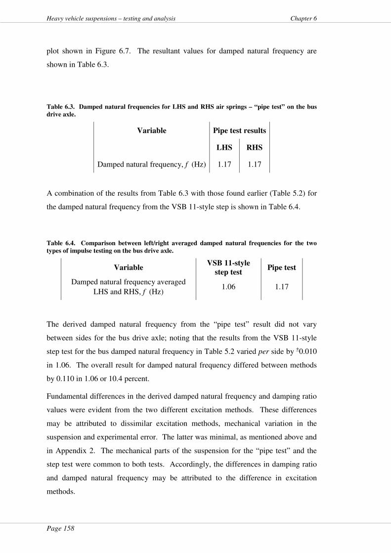
Page 158
Heavy vehicle suspensions – testing and analysis Chapter 6
plot shown in Figure 6.7. The resultant values for damped natural frequency are
shown in Table 6.3.
Table 6.3. Damped natural frequencies for LHS and RHS air springs – “pipe test” on the bus
drive axle.
Variable Pipe test results
LHS RHS
Damped natural frequency, f (Hz) 1.17 1.17
A combination of the results from Table 6.3 with those found earlier (Table 5.2) for
the damped natural frequency from the VSB 11-style step is shown in Table 6.4.
Table 6.4. Comparison between left/right averaged damped natural frequencies for the two
types of impulse testing on the bus drive axle.
Variable VSB 11-style
step test Pipe test
Damped natural frequency averaged
LHS and RHS, f (Hz) 1.06 1.17
The derived damped natural frequency from the “pipe test” result did not vary
between sides for the bus drive axle; noting that the results from the VSB 11-style
step test for the bus damped natural frequency in Table 5.2 varied per side by +0.010
in 1.06. The overall result for damped natural frequency differed between methods
by 0.110 in 1.06 or 10.4 percent.
Fundamental differences in the derived damped natural frequency and damping ratio
values were evident from the two different excitation methods. These differences
may be attributed to dissimilar excitation methods, mechanical variation in the
suspension and experimental error. The latter was minimal, as mentioned above and
in Appendix 2. The mechanical parts of the suspension for the “pipe test” and the
step test were common to both tests. Accordingly, the differences in damping ratio
and damped natural frequency may be attributed to the difference in excitation
methods.
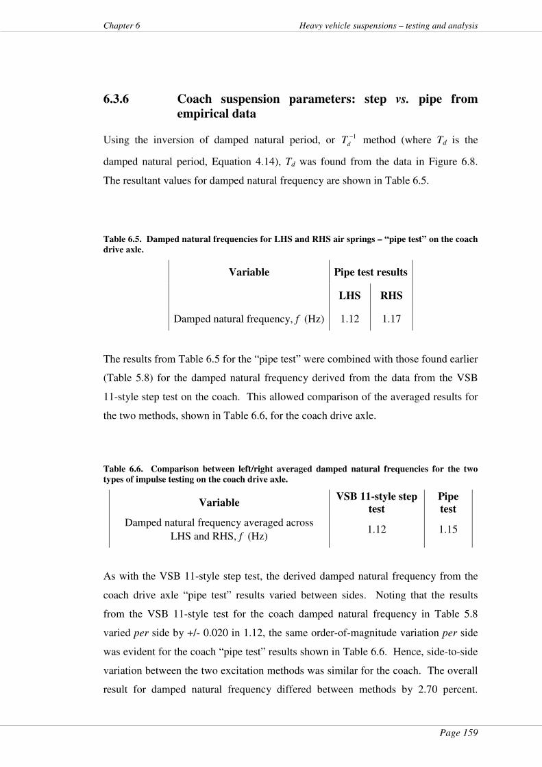
Page 159
Chapter 6 Heavy vehicle suspensions – testing and analysis
6.3.6 Coach suspension parameters: step vs. pipe from
empirical data
Using the inversion of damped natural period, or 1−dT method (where Td is the
damped natural period, Equation 4.14), Td was found from the data in Figure 6.8.
The resultant values for damped natural frequency are shown in Table 6.5.
Table 6.5. Damped natural frequencies for LHS and RHS air springs – “pipe test” on the coach
drive axle.
Variable Pipe test results
LHS RHS
Damped natural frequency, f (Hz) 1.12 1.17
The results from Table 6.5 for the “pipe test” were combined with those found earlier
(Table 5.8) for the damped natural frequency derived from the data from the VSB
11-style step test on the coach. This allowed comparison of the averaged results for
the two methods, shown in Table 6.6, for the coach drive axle.
Table 6.6. Comparison between left/right averaged damped natural frequencies for the two
types of impulse testing on the coach drive axle.
Variable VSB 11-style step
test
Pipe
test
Damped natural frequency averaged across
LHS and RHS, f (Hz) 1.12 1.15
As with the VSB 11-style step test, the derived damped natural frequency from the
coach drive axle “pipe test” results varied between sides. Noting that the results
from the VSB 11-style test for the coach damped natural frequency in Table 5.8
varied per side by +/- 0.020 in 1.12, the same order-of-magnitude variation per side
was evident for the coach “pipe test” results shown in Table 6.6. Hence, side-to-side
variation between the two excitation methods was similar for the coach. The overall
result for damped natural frequency differed between methods by 2.70 percent.
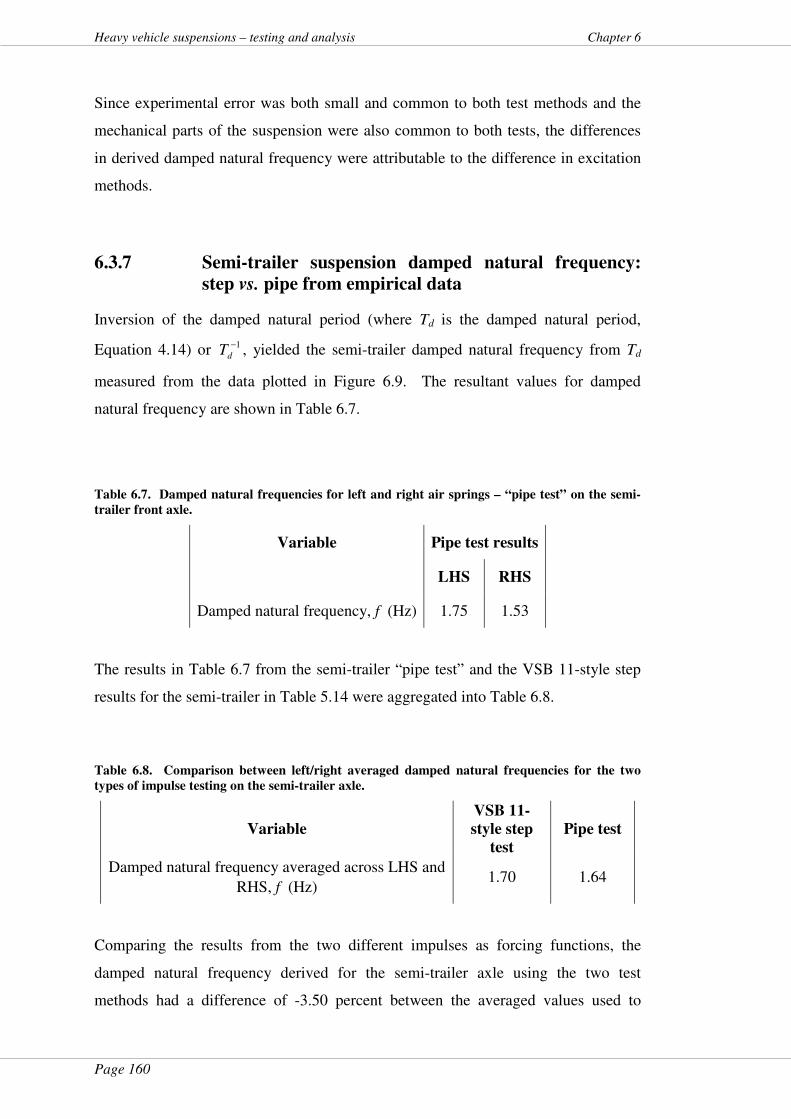
Page 160
Heavy vehicle suspensions – testing and analysis Chapter 6
Since experimental error was both small and common to both test methods and the
mechanical parts of the suspension were also common to both tests, the differences
in derived damped natural frequency were attributable to the difference in excitation
methods.
6.3.7 Semi-trailer suspension damped natural frequency:
step vs. pipe from empirical data
Inversion of the damped natural period (where Td is the damped natural period,
Equation 4.14) or 1−dT , yielded the semi-trailer damped natural frequency from Td
measured from the data plotted in Figure 6.9. The resultant values for damped
natural frequency are shown in Table 6.7.
Table 6.7. Damped natural frequencies for left and right air springs – “pipe test” on the semi-
trailer front axle.
Variable Pipe test results
LHS RHS
Damped natural frequency, f (Hz) 1.75 1.53
The results in Table 6.7 from the semi-trailer “pipe test” and the VSB 11-style step
results for the semi-trailer in Table 5.14 were aggregated into Table 6.8.
Table 6.8. Comparison between left/right averaged damped natural frequencies for the two
types of impulse testing on the semi-trailer axle.
Variable
VSB 11-
style step
test
Pipe test
Damped natural frequency averaged across LHS and
RHS, f (Hz) 1.70 1.64
Comparing the results from the two different impulses as forcing functions, the
damped natural frequency derived for the semi-trailer axle using the two test
methods had a difference of -3.50 percent between the averaged values used to
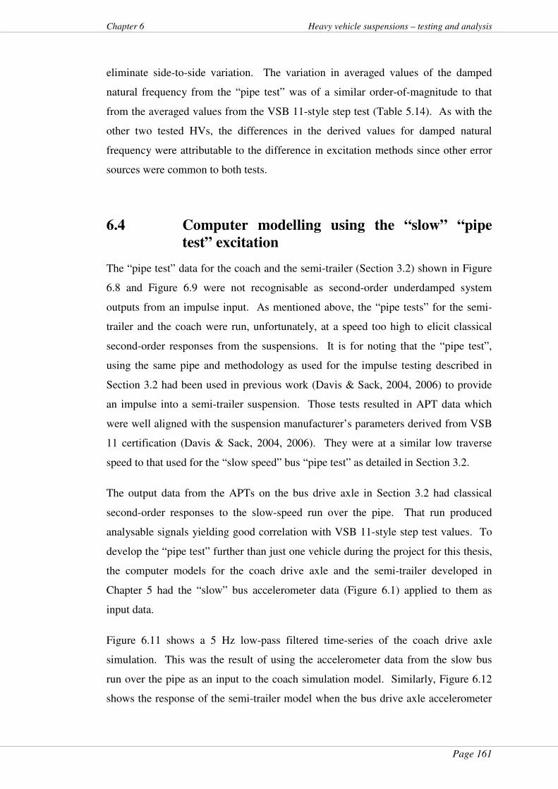
Page 161
Chapter 6 Heavy vehicle suspensions – testing and analysis
eliminate side-to-side variation. The variation in averaged values of the damped
natural frequency from the “pipe test” was of a similar order-of-magnitude to that
from the averaged values from the VSB 11-style step test (Table 5.14). As with the
other two tested HVs, the differences in the derived values for damped natural
frequency were attributable to the difference in excitation methods since other error
sources were common to both tests.
6.4 Computer modelling using the “slow” “pipe
test” excitation
The “pipe test” data for the coach and the semi-trailer (Section 3.2) shown in Figure
6.8 and Figure 6.9 were not recognisable as second-order underdamped system
outputs from an impulse input. As mentioned above, the “pipe tests” for the semi-
trailer and the coach were run, unfortunately, at a speed too high to elicit classical
second-order responses from the suspensions. It is for noting that the “pipe test”,
using the same pipe and methodology as used for the impulse testing described in
Section 3.2 had been used in previous work (Davis & Sack, 2004, 2006) to provide
an impulse into a semi-trailer suspension. Those tests resulted in APT data which
were well aligned with the suspension manufacturer’s parameters derived from VSB
11 certification (Davis & Sack, 2004, 2006). They were at a similar low traverse
speed to that used for the “slow speed” bus “pipe test” as detailed in Section 3.2.
The output data from the APTs on the bus drive axle in Section 3.2 had classical
second-order responses to the slow-speed run over the pipe. That run produced
analysable signals yielding good correlation with VSB 11-style step test values. To
develop the “pipe test” further than just one vehicle during the project for this thesis,
the computer models for the coach drive axle and the semi-trailer developed in
Chapter 5 had the “slow” bus accelerometer data (Figure 6.1) applied to them as
input data.
Figure 6.11 shows a 5 Hz low-pass filtered time-series of the coach drive axle
simulation. This was the result of using the accelerometer data from the slow bus
run over the pipe as an input to the coach simulation model. Similarly, Figure 6.12
shows the response of the semi-trailer model when the bus drive axle accelerometer

Page 162
Heavy vehicle suspensions – testing and analysis Chapter 6
data were used as the input.
3 3.5 4 4.5 5 5.5 6 6.5 7-100
-50
0
50
100
150model suspension response to pipe test empirical data input
time (s)
Magnitude o
f sim
ula
ted s
uspensio
n r
esponse (
arb
itra
ry lin
ear
scale
)
Figure 6.11. Time series of Matlab Simulink model of coach drive axle APT output for
empirical coach hub vertical acceleration input during “pipe test”.
4 4.5 5 5.5 6 6.5 7 7.5 8-100
-50
0
50
100
150model suspension response to pipe test empirical data input
time (s)
Magnitude o
f sim
ula
ted s
uspensio
n r
esponse (
arb
itra
ry lin
ear
scale
)
Figure 6.12. Time series of Matlab Simulink model of semi-trailer axle APT output for
empirical trailer front hub vertical acceleration input during “pipe test”.

Page 163
Chapter 6 Heavy vehicle suspensions – testing and analysis
Damping ratios and damped natural frequencies were derived from the data in Figure
6.11 and Figure 6.12; the coach drive axle and the semi-trailer axle model outputs
using the slow bus traverse over the pipe as the input. These were derived using
Equation 4.18 and Equation 4.14 respectively, as before. These values are shown in
Table 6.9 and Table 6.10.
Table 6.9. Comparison of simulation models’ damping ratios for the slow “pipe test” vs. VSB
11-style test values.
Variable
Coach model using
empirical input data
from the slow “pipe
test”
Semi-trailer model
using empirical input
data from the slow
“pipe test”
Quiescent signal value 5.96 0
A1 117 103
A2 21.8 19.1
Damping ratio, ζ 0.297 0.259
Error compared with average of actual VSB
11-style step test
damping ratio, ζ
-17.5% 3.60%
The results summarised in Table 6.9 indicated that the semi-trailer model, when
presented with the “slow” “pipe test” as an input, yielded a damping ratio that varied
from the empirically derived VSB11-style step test result for damping ratio by 3.6
percent. This was the same order-of-magnitude error for the models when empirical
VSB 11-style step test data were used as inputs (Table 5.19 to Table 5.21).
The derived damping ratio from the coach drive axle model with the slow “pipe test”
had an error of -17.5 percent compared with the derived result for damping ratio
from the VSB 11-style step test. This result indicated that the “pipe test” needed to
be considered further, including the appreciable error in the derived coach damping
ratio.
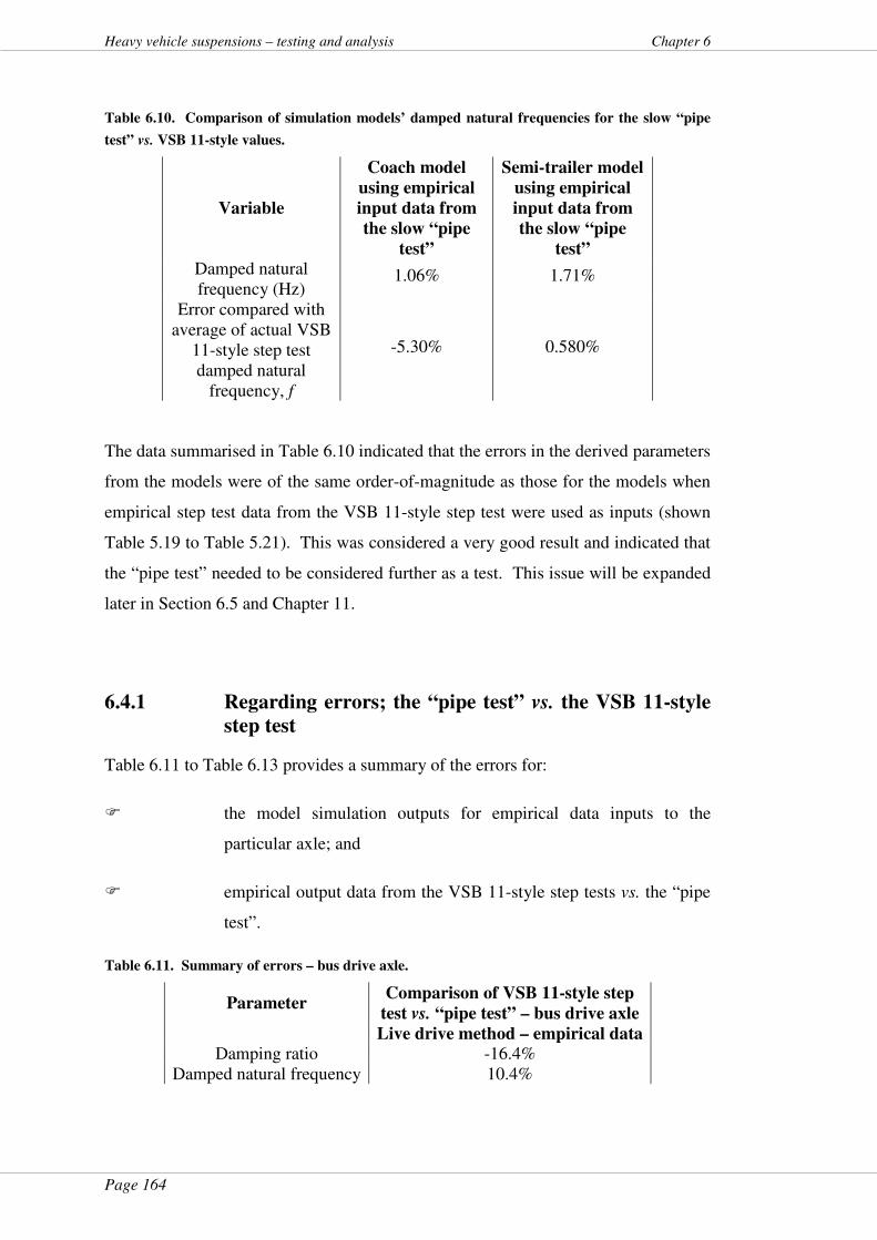
Page 164
Heavy vehicle suspensions – testing and analysis Chapter 6
Table 6.10. Comparison of simulation models’ damped natural frequencies for the slow “pipe
test” vs. VSB 11-style values.
Variable
Coach model
using empirical
input data from
the slow “pipe
test”
Semi-trailer model
using empirical
input data from
the slow “pipe
test” Damped natural frequency (Hz)
1.06% 1.71%
Error compared with average of actual VSB
11-style step test damped natural
frequency, f
-5.30% 0.580%
The data summarised in Table 6.10 indicated that the errors in the derived parameters
from the models were of the same order-of-magnitude as those for the models when
empirical step test data from the VSB 11-style step test were used as inputs (shown
Table 5.19 to Table 5.21). This was considered a very good result and indicated that
the “pipe test” needed to be considered further as a test. This issue will be expanded
later in Section 6.5 and Chapter 11.
6.4.1 Regarding errors; the “pipe test” vs. the VSB 11-style
step test
Table 6.11 to Table 6.13 provides a summary of the errors for:
� the model simulation outputs for empirical data inputs to the
particular axle; and
� empirical output data from the VSB 11-style step tests vs. the “pipe
test”.
Table 6.11. Summary of errors – bus drive axle.
Parameter Comparison of VSB 11-style step
test vs. “pipe test” – bus drive axle
Live drive method – empirical data Damping ratio -16.4%
Damped natural frequency 10.4%

Page 165
Chapter 6 Heavy vehicle suspensions – testing and analysis
The “pipe test” input signals from Figure 5.3 to Figure 5.5 may be compared with the
VSB 11-style step down test input signals shown from Figure 6.1 to Figure 6.3. The
“pipe test”, when compared with the VSB 11 step down test:
� imparted a similarly shaped time-domain impulse into HV suspensions;
� imparted the required impulse for a comparable time; and
� had a similar amplitude at the axles.
The discontinuity provided by the pipe was sufficient to provide an impulse of the
appropriate characteristics and equivalent to that of the step down test used in VSB
11 to excite a HV suspension. The results, from actual experimental data, of the
response to the “pipe test” input were sufficient to yield dynamic suspension
parameters with a worst-case error of approximately 16 percent (Table 6.11) for the
damping ratio.
Table 6.12. Summary of errors – coach drive axle.
Parameter Comparison of VSB 11-style step test vs. “pipe test” –
coach drive axle
Live drive method –
empirical data
Using bus “pipe test” data as
input
vs. VSB 11 empirical result Damping ratio n/a -17.5%
Damped natural frequency
2.70% -5.30%
This was for the “pipe test” case when compared with the VSB 11-derived
parameters, since manufacturer’s parameters were not available. Further, any errors
were within this same margin as the results for VSB 11-style tests conducted
contemporaneously with the “pipe tests”.
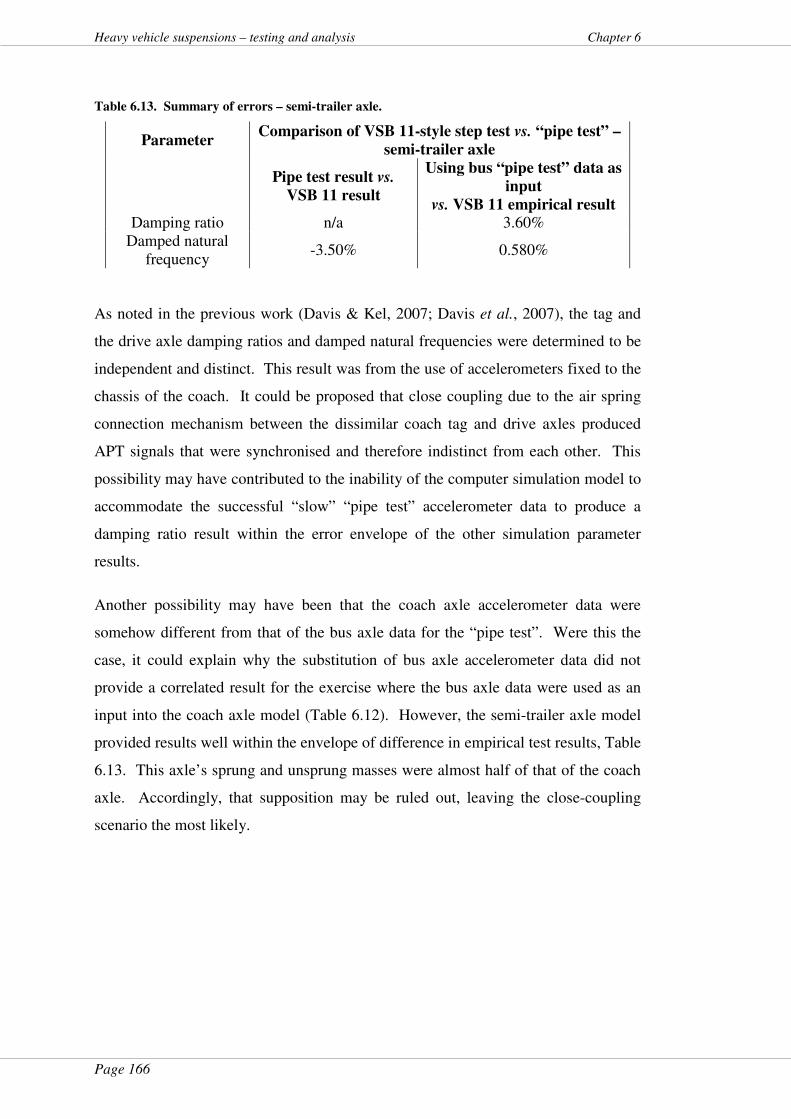
Page 166
Heavy vehicle suspensions – testing and analysis Chapter 6
Table 6.13. Summary of errors – semi-trailer axle.
Parameter Comparison of VSB 11-style step test vs. “pipe test” –
semi-trailer axle
Pipe test result vs.
VSB 11 result
Using bus “pipe test” data as
input
vs. VSB 11 empirical result Damping ratio n/a 3.60%
Damped natural frequency
-3.50% 0.580%
As noted in the previous work (Davis & Kel, 2007; Davis et al., 2007), the tag and
the drive axle damping ratios and damped natural frequencies were determined to be
independent and distinct. This result was from the use of accelerometers fixed to the
chassis of the coach. It could be proposed that close coupling due to the air spring
connection mechanism between the dissimilar coach tag and drive axles produced
APT signals that were synchronised and therefore indistinct from each other. This
possibility may have contributed to the inability of the computer simulation model to
accommodate the successful “slow” “pipe test” accelerometer data to produce a
damping ratio result within the error envelope of the other simulation parameter
results.
Another possibility may have been that the coach axle accelerometer data were
somehow different from that of the bus axle data for the “pipe test”. Were this the
case, it could explain why the substitution of bus axle accelerometer data did not
provide a correlated result for the exercise where the bus axle data were used as an
input into the coach axle model (Table 6.12). However, the semi-trailer axle model
provided results well within the envelope of difference in empirical test results, Table
6.13. This axle’s sprung and unsprung masses were almost half of that of the coach
axle. Accordingly, that supposition may be ruled out, leaving the close-coupling
scenario the most likely.
Page 167
Chapter 6 Heavy vehicle suspensions – testing and analysis
6.5 Summary of this chapter
6.5.1 General
This section summarises the results and analysis detailed in this chapter in
preparation for a discussion in Chapter 11.
6.5.2 The “pipe test” vs. VSB 11-style step test - duration
VSB 11 (Australia Department of Transport and Regional Services, 2004a) defines
testing of heavy vehicle (HV) suspensions for “road friendliness”. The step test is
one VSB 11 method for an impulse to be imparted to a HV suspension; the tyre is
rolled off an 80mm step. The resultant axle-to-chassis transient signal is then
measured and analysed for damping ratio and damped natural sprung mass
frequency. This action is akin to characterising a control system by the application
of an impulse as a forcing function (Chesmond, 1982; Doebelin, 1980).
The time taken by a HV tyre to execute the VSB 11 specified step is finite. Figure
5.3 to Figure 5.5 shows that this time was approximately 0.4 to 0.5 s. Similarly, the
impulse duration from the “pipe test” shown from Figure 6.1 to Figure 6.3 is also
approximately 0.4 to 0.5 s. Previous work provided a theoretical study of the
duration of the impulse signal from the “pipe test” (Davis & Sack, 2006) . That
theoretical work predicted 0.43 s impulse duration at the axle for an 11R22.5 tyre
and a 50 mm steel pipe and allowed for tyre enveloping using a point-follower
model. The validation of this work was in the match between the impulse lengths
from the theoretical study and the empirical data. Accordingly, a combination of:
� 5 km/h approach speed, and
� traverse over a 50 mm pipe
would provide an impulse of sufficient signal strength and duration to allow the
resultant signal at a HV spring to be analysed for body bounce frequency and
damping ratio.

Page 168
Heavy vehicle suspensions – testing and analysis Chapter 6
6.5.3 The “pipe test” vs. VSB 11-style step test - errors
The error summary shown from Table 6.11 to Table 6.13 indicated that the
maximum error between “live drive” “pipe test” results and empirical VSB 11-style
step test results was approximately 16 percent and this for the damping ratio.
Damped natural frequency error between the two test methods was approximately 10
percent. Damped natural frequency is dependent on air spring size and suspension
geometry and does not change that much in service (Blanksby et al., 2006; Patrick et
al., 2009). Frequency has a component that is proportional to ( )211 ζ− as
detailed in Equation 4.16. Accordingly, halving the damping ratio from (say) 0.2 to
0.1 alters the frequency by 1.5 percent. The damping ratio on the other hand, being
dependent on damper health, changes with time (Blanksby et al., 2006); any
alterations to shock absorber performance affect the damping directly and
proportionally, as detailed in Chapter 5. Accordingly, damping ratio may be
considered to be the most critical (and dependent on damper health) of the two
parameters that define a RFS. The error values found for this test programme, when
determining damping ratio values in particular, were surprisingly low since previous
researchers noted difficulty in determining this parameter accurately (Woodrooffe,
1995) and others who noted a 60 percent difference in derived results, depending on
method (Prem et al., 1998; Uffelmann & Walter, 1994). The work of Uffelmann and
Walter (1994) examined the potential for measured parameter values to differ, even
when derived from the same suspension. The conclusion from that work was that
these differences derived directly from, and were dependent on, excitation method;
the damping ratio derived from a “pull down and release” type impulse to a HV
suspension differed 42 percent from the damping ratio derived from the same
suspension subjected to a “lift and drop” impulse. It is noted that both of these
methods are allowed under VSB 11. Further, VSB 11 testing in Australia does not
generally involve multi-axle groups (Section 11.3.1). The pipe test, provided the
traverse speeds are constrained within a manageable but narrow band, would allow
multi-axle groups to be tested within an in-service environment.
Page 169
Chapter 6 Heavy vehicle suspensions – testing and analysis
6.5.4 The “pipe test” vs. VSB 11-style step test – need for
development
As mentioned in the introduction to this chapter, the “pipe tests” undertaken for this
project were singular occurrences. Different project funding and logistical
arrangements may have facilitated multiple runs over the pipe and step tests resulting
in analysis for statistical significance.
As the results stand, they are a “proof-of-concept” only. Nonetheless, previous work
in an earlier Main Roads project performed multiple runs over the “pipe test” (Davis
& Sack, 2006). The results for that programme indicated that errors between the
“pipe test” and the manufacturer’s VSB 11 specifications varied by no more than 14
percent for frequency and 12 percent for damping ratio, similar to the results detailed
in this chapter.
6.6 Chapter close
6.6.1 General
Chapter 3 described two methodologies for low cost testing of HV suspension. One
was the “pipe test” where a heavy vehicle (HV) wheel was rolled over a 50 mm steel
pipe at low speed with the air spring response measured. Those test procedures have
been analysed in this chapter.
The models developed in Chapter 5, previously validated against empirical data for
damped natural frequency and damping ratio, were used to determine the validity of
the low cost “pipe test” method in this chapter.
Chapter 12 will use the semi-trailer axle model developed in this chapter. Three of
the axle models in Figure 5.13 will be formed into a tri-axle group. This meta-model
will be used to explore the ability of a simulated semi-trailer group to distribute load
at the air springs for varying levels of air line connectivity between axles.
Accordingly, the models developed and validated in this chapter will allow
exploration of the theoretical limits of air spring suspension load sharing in Chapter
12.
Page 170
Heavy vehicle suspensions – testing and analysis Chapter 6
Links where this chapter informs other chapters of this thesis are shown in Figure
1.4.
“Public opinion in 1491 held that the world was flat - no progress without analysis.”
Page 171
Chapter 7 Heavy vehicle suspensions – testing and analysis
7 Data analysis - on road testing and roller
bed
7.1 About this chapter
This chapter presents analysis of the data from the roller bed testing detailed in
Section 3.3. This was to inform the remainder of Objective 3 of this project; a low
cost suspension test. This chapter also presents the results and analysis of empirical
dynamic wheel forces from the on-road testing (Section 3.2.2) in terms of test speeds
and a “novel roughness” measure developed for this project. These are presented as
an innovative contribution to the project’s body of knowledge and for use in Chapter
10 in evaluating the changes to air sprung heavy vehicle (HV) suspensions from
larger longitudinal air lines.
7.2 Introduction
As detailed in Chapter 1, Sections 1.4 and 1.7.3, a low cost suspension test was
developed to meet Objective 3 of this project; development of a low cost suspension
tester. The results from the roller bed testing data gathered as described in Section
3.3 were analysed. These, as well as analysis of the data gathered from the on-road
testing detailed in Section 3.2.2 are presented. A useful outcome was evident from
this analysis; the ability to show dynamic wheel forces measured against speed and
roughness values for the test roads used. These dynamic forces vs. a “novel
roughness” value (also denoted a “novel roughness” measure), developed for this
project, are documented in this chapter.
7.3 Wheel forces vs. roughness
7.3.1 “Novel roughness” metric - derivation
As mentioned in Section 3.2.7, road roughness is usually designated by a standard
measure, the international roughness index (IRI), found using calibrated vehicles.
The units of this roughness measure are mm/m or m/km. IRI indicates an amount of
vertical movement relative to travelled horizontal distance. This roughness measure
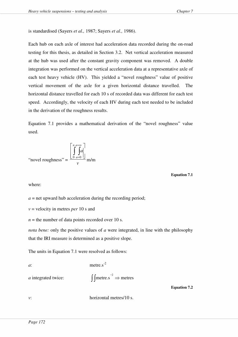
Page 172
Heavy vehicle suspensions – testing and analysis Chapter 7
is standardised (Sayers et al., 1987; Sayers et al., 1986).
Each hub on each axle of interest had acceleration data recorded during the on-road
testing for this thesis, as detailed in Section 3.2. Net vertical acceleration measured
at the hub was used after the constant gravity component was removed. A double
integration was performed on the vertical acceleration data at a representative axle of
each test heavy vehicle (HV). This yielded a “novel roughness” value of positive
vertical movement of the axle for a given horizontal distance travelled. The
horizontal distance travelled for each 10 s of recorded data was different for each test
speed. Accordingly, the velocity of each HV during each test needed to be included
in the derivation of the roughness results.
Equation 7.1 provides a mathematical derivation of the “novel roughness” value
used.
“novel roughness” = v
a
n a
a
∫ ∫∞=
=0 0m/m
Equation 7.1
where:
a = net upward hub acceleration during the recording period;
v = velocity in metres per 10 s and
n = the number of data points recorded over 10 s.
nota bene: only the positive values of a were integrated, in line with the philosophy
that the IRI measure is determined as a positive slope.
The units in Equation 7.1 were resolved as follows:
a: metre.s-2
a integrated twice: metresmetre.s2
⇒−
∫ ∫
Equation 7.2
v: horizontal metres/10 s.
Page 173
Chapter 7 Heavy vehicle suspensions – testing and analysis
Equation 7.2 provided the transformation of measured acceleration into the positive
vertical displacement (in metres) that the hubs moved during the 10 s recording
period (vertical metres/10 s) per test run. Returning to Equation 7.1, the units of
“novel roughness” from Equation 7.1 may then be resolved:
“novel roughness” units = v
af ][ =
metres/10s horizontal
s metres/10 vertical =
metres horizontal
metres vertical
A factor of 1000 was applied to render this “novel roughness” value into mm/m.
This “novel roughness” value or “novel roughness” measure should not be equated to
the IRI value of the roads used for the testing. It was derived to provide an indicative
measure of roughness as experienced by each test HV axle at a representative hub
accelerometer. The tyres, axle mass and wheel mass varied with each test vehicle.
Accordingly, the “novel roughness” value derived was unique to each vehicle. It
arose from the contributions of the unsprung mass dynamics combined with those
from surface irregularities. In this way, it was similar to the methodology for
determining IRI; that methodology does not distinguish between contributory forces
from the axle-to-body dynamics of the test vehicle compared with those from the
surface irregularities of the pavement (Sayers et al., 1987; Sayers et al., 1986). Even
so, the “novel roughness” value provided an independent variable against which to
plot wheel force as the dependent variable.
7.3.2 “Novel roughness” vs. wheel load
The data plotted from Figure 7.1 to Figure 7.9 show the peaks, standard deviations
and means of the wheel forces vs. “novel roughness” values for each test vehicle axle
of interest. The drive axle of the coach and the front axle of the semi-trailer were
chosen as the axles of interest for those HVs for the plots. The coach drive axle was
chosen as its forces were higher (and therefore potentially more damaging) than the
tag axle of the coach. The semi-trailer’s front axle plots were very similar to its other
axles.
A brief commentary is provided, where appropriate, on each figure in the sections on
the bus, coach and semi-trailer below.
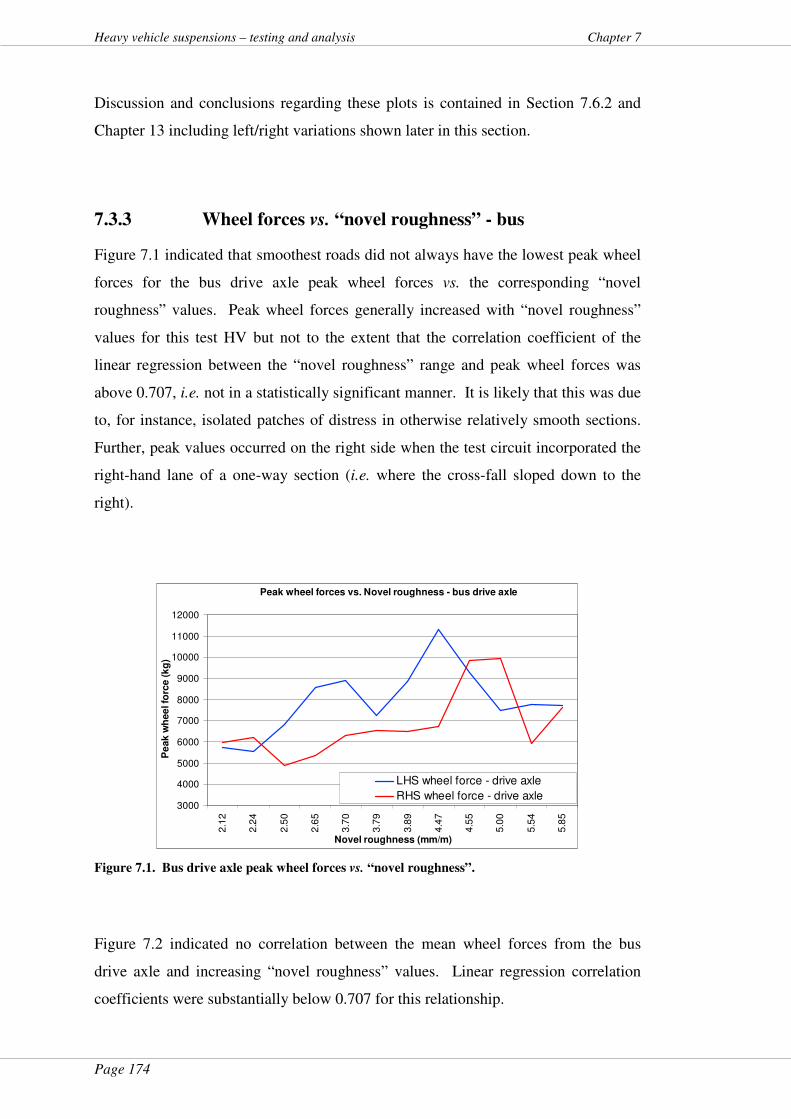
Page 174
Heavy vehicle suspensions – testing and analysis Chapter 7
Discussion and conclusions regarding these plots is contained in Section 7.6.2 and
Chapter 13 including left/right variations shown later in this section.
7.3.3 Wheel forces vs. “novel roughness” - bus
Figure 7.1 indicated that smoothest roads did not always have the lowest peak wheel
forces for the bus drive axle peak wheel forces vs. the corresponding “novel
roughness” values. Peak wheel forces generally increased with “novel roughness”
values for this test HV but not to the extent that the correlation coefficient of the
linear regression between the “novel roughness” range and peak wheel forces was
above 0.707, i.e. not in a statistically significant manner. It is likely that this was due
to, for instance, isolated patches of distress in otherwise relatively smooth sections.
Further, peak values occurred on the right side when the test circuit incorporated the
right-hand lane of a one-way section (i.e. where the cross-fall sloped down to the
right).
Peak wheel forces vs. Novel roughness - bus drive axle
3000
4000
5000
6000
7000
8000
9000
10000
11000
12000
2.1
2
2.2
4
2.5
0
2.6
5
3.7
0
3.7
9
3.8
9
4.4
7
4.5
5
5.0
0
5.5
4
5.8
5
Novel roughness (mm/m)
Pe
ak w
hee
l fo
rce
(k
g)
LHS wheel force - drive axle
RHS wheel force - drive axle
Figure 7.1. Bus drive axle peak wheel forces vs. “novel roughness”.
Figure 7.2 indicated no correlation between the mean wheel forces from the bus
drive axle and increasing “novel roughness” values. Linear regression correlation
coefficients were substantially below 0.707 for this relationship.
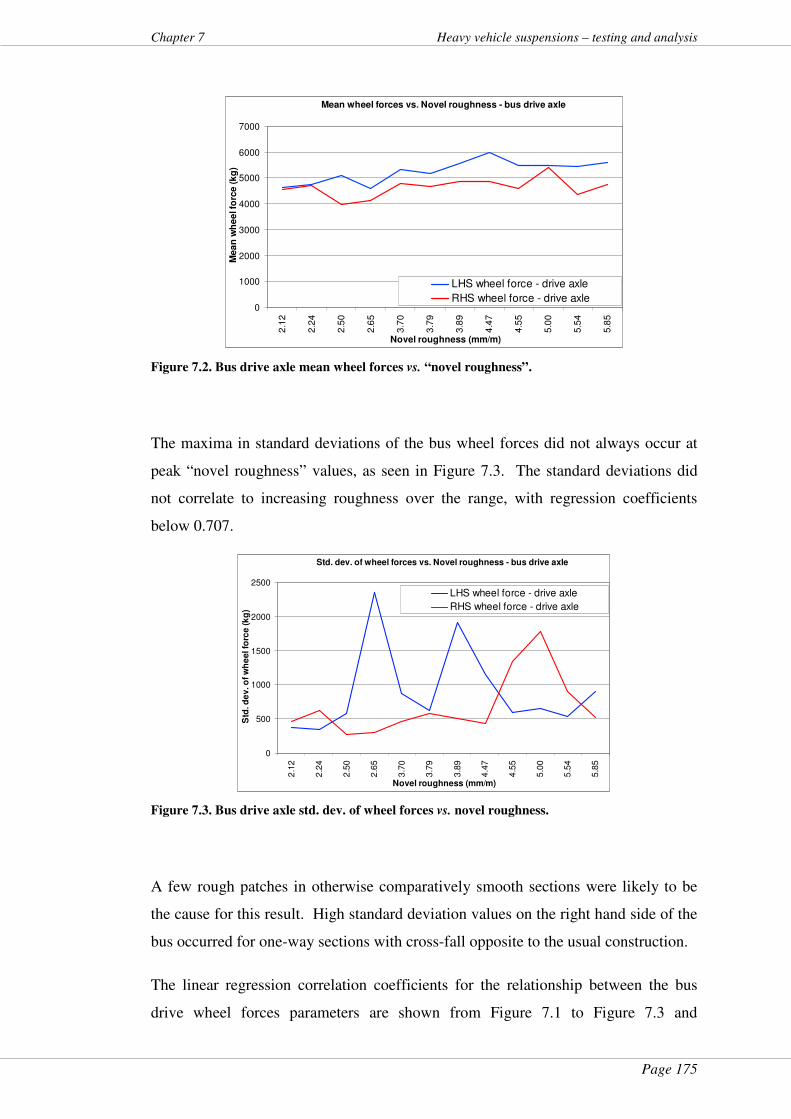
Page 175
Chapter 7 Heavy vehicle suspensions – testing and analysis
Mean wheel forces vs. Novel roughness - bus drive axle
0
1000
2000
3000
4000
5000
6000
7000
2.1
2
2.2
4
2.5
0
2.6
5
3.7
0
3.7
9
3.8
9
4.4
7
4.5
5
5.0
0
5.5
4
5.8
5
Novel roughness (mm/m)
Mea
n w
he
el fo
rce
(k
g)
LHS wheel force - drive axle
RHS wheel force - drive axle
Figure 7.2. Bus drive axle mean wheel forces vs. “novel roughness”.
The maxima in standard deviations of the bus wheel forces did not always occur at
peak “novel roughness” values, as seen in Figure 7.3. The standard deviations did
not correlate to increasing roughness over the range, with regression coefficients
below 0.707.
Std. dev. of wheel forces vs. Novel roughness - bus drive axle
0
500
1000
1500
2000
2500
2.1
2
2.2
4
2.5
0
2.6
5
3.7
0
3.7
9
3.8
9
4.4
7
4.5
5
5.0
0
5.5
4
5.8
5
Novel roughness (mm/m)
Std
. d
ev. o
f w
he
el fo
rce (
kg
)
LHS wheel force - drive axle
RHS wheel force - drive axle
Figure 7.3. Bus drive axle std. dev. of wheel forces vs. novel roughness.
A few rough patches in otherwise comparatively smooth sections were likely to be
the cause for this result. High standard deviation values on the right hand side of the
bus occurred for one-way sections with cross-fall opposite to the usual construction.
The linear regression correlation coefficients for the relationship between the bus
drive wheel forces parameters are shown from Figure 7.1 to Figure 7.3 and
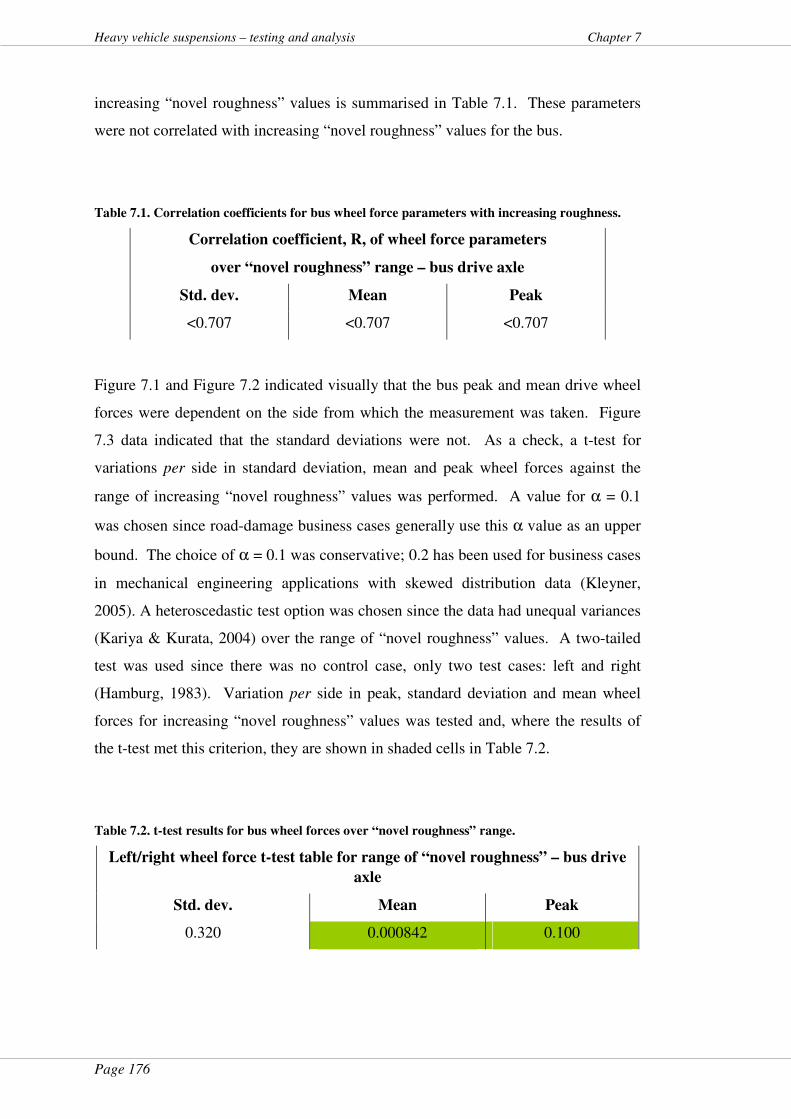
Page 176
Heavy vehicle suspensions – testing and analysis Chapter 7
increasing “novel roughness” values is summarised in Table 7.1. These parameters
were not correlated with increasing “novel roughness” values for the bus.
Table 7.1. Correlation coefficients for bus wheel force parameters with increasing roughness.
Correlation coefficient, R, of wheel force parameters
over “novel roughness” range – bus drive axle
Std. dev. Mean Peak
<0.707 <0.707 <0.707
Figure 7.1 and Figure 7.2 indicated visually that the bus peak and mean drive wheel
forces were dependent on the side from which the measurement was taken. Figure
7.3 data indicated that the standard deviations were not. As a check, a t-test for
variations per side in standard deviation, mean and peak wheel forces against the
range of increasing “novel roughness” values was performed. A value for α = 0.1
was chosen since road-damage business cases generally use this α value as an upper
bound. The choice of α = 0.1 was conservative; 0.2 has been used for business cases
in mechanical engineering applications with skewed distribution data (Kleyner,
2005). A heteroscedastic test option was chosen since the data had unequal variances
(Kariya & Kurata, 2004) over the range of “novel roughness” values. A two-tailed
test was used since there was no control case, only two test cases: left and right
(Hamburg, 1983). Variation per side in peak, standard deviation and mean wheel
forces for increasing “novel roughness” values was tested and, where the results of
the t-test met this criterion, they are shown in shaded cells in Table 7.2.
Table 7.2. t-test results for bus wheel forces over “novel roughness” range.
Left/right wheel force t-test table for range of “novel roughness” – bus drive
axle
Std. dev. Mean Peak
0.320 0.000842 0.100
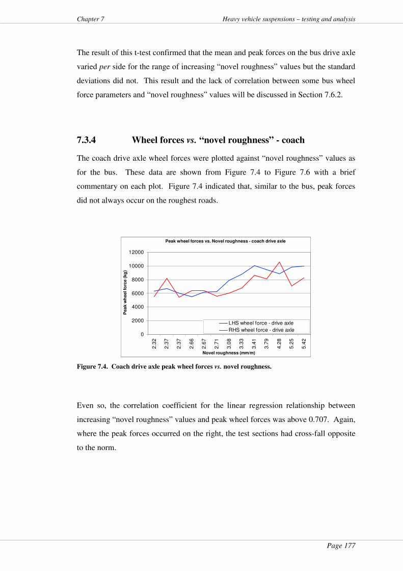
Page 177
Chapter 7 Heavy vehicle suspensions – testing and analysis
The result of this t-test confirmed that the mean and peak forces on the bus drive axle
varied per side for the range of increasing “novel roughness” values but the standard
deviations did not. This result and the lack of correlation between some bus wheel
force parameters and “novel roughness” values will be discussed in Section 7.6.2.
7.3.4 Wheel forces vs. “novel roughness” - coach
The coach drive axle wheel forces were plotted against “novel roughness” values as
for the bus. These data are shown from Figure 7.4 to Figure 7.6 with a brief
commentary on each plot. Figure 7.4 indicated that, similar to the bus, peak forces
did not always occur on the roughest roads.
Peak wheel forces vs. Novel roughness - coach drive axle
0
2000
4000
6000
8000
10000
12000
2.3
2
2.3
7
2.3
7
2.6
6
2.6
7
2.7
1
3.0
8
3.3
3
3.4
1
3.7
9
4.2
8
5.2
5
5.4
2
Novel roughness (mm/m)
Pea
k w
heel fo
rce
(kg
)
LHS wheel force - drive axle
RHS wheel force - drive axle
Figure 7.4. Coach drive axle peak wheel forces vs. novel roughness.
Even so, the correlation coefficient for the linear regression relationship between
increasing “novel roughness” values and peak wheel forces was above 0.707. Again,
where the peak forces occurred on the right, the test sections had cross-fall opposite
to the norm.
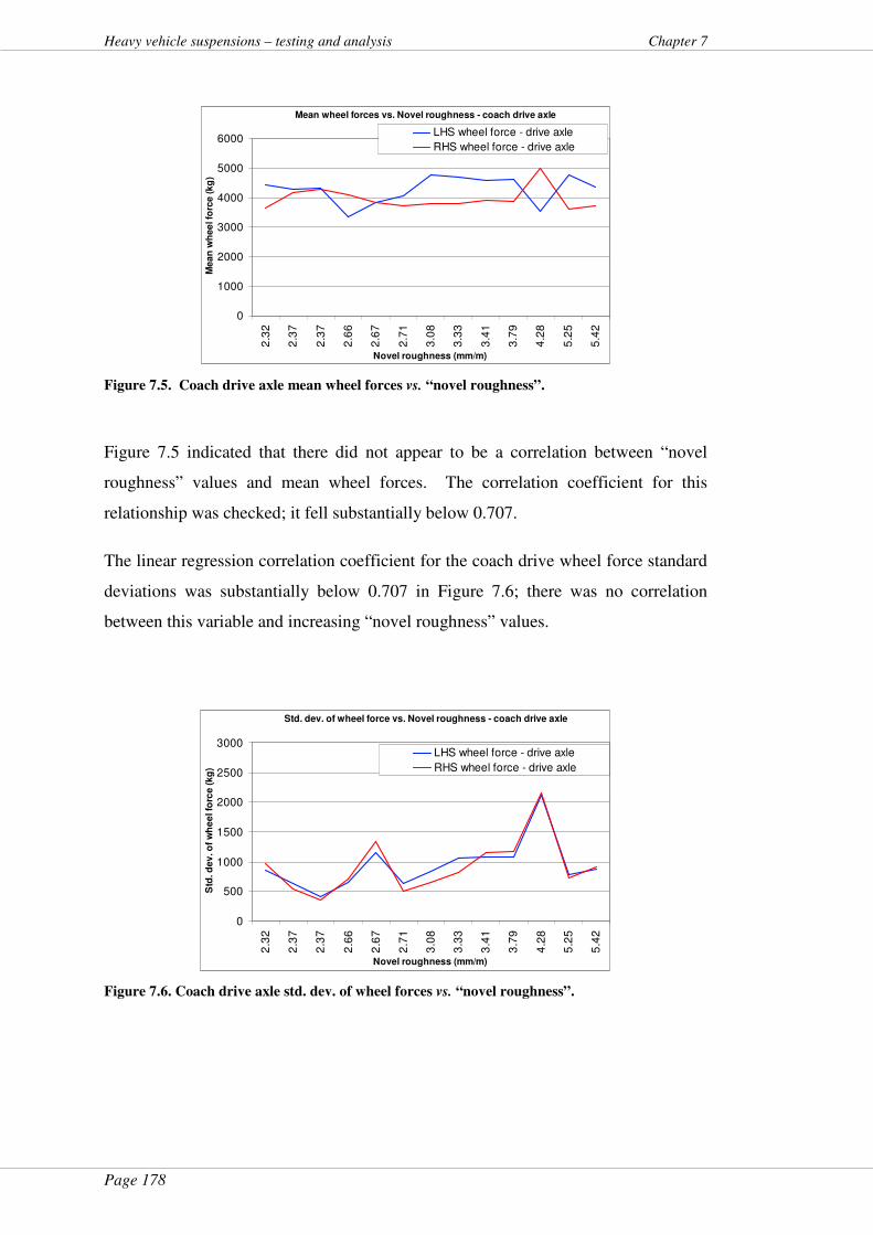
Page 178
Heavy vehicle suspensions – testing and analysis Chapter 7
Mean wheel forces vs. Novel roughness - coach drive axle
0
1000
2000
3000
4000
5000
6000
2.3
2
2.3
7
2.3
7
2.6
6
2.6
7
2.7
1
3.0
8
3.3
3
3.4
1
3.7
9
4.2
8
5.2
5
5.4
2
Novel roughness (mm/m)
Me
an
wh
ee
l fo
rce
(k
g)
LHS wheel force - drive axle
RHS wheel force - drive axle
Figure 7.5. Coach drive axle mean wheel forces vs. “novel roughness”.
Figure 7.5 indicated that there did not appear to be a correlation between “novel
roughness” values and mean wheel forces. The correlation coefficient for this
relationship was checked; it fell substantially below 0.707.
The linear regression correlation coefficient for the coach drive wheel force standard
deviations was substantially below 0.707 in Figure 7.6; there was no correlation
between this variable and increasing “novel roughness” values.
Std. dev. of wheel force vs. Novel roughness - coach drive axle
0
500
1000
1500
2000
2500
3000
2.3
2
2.3
7
2.3
7
2.6
6
2.6
7
2.7
1
3.0
8
3.3
3
3.4
1
3.7
9
4.2
8
5.2
5
5.4
2
Novel roughness (mm/m)
Std
. d
ev
. o
f w
he
el fo
rce (
kg
)
LHS wheel force - drive axle
RHS wheel force - drive axle
Figure 7.6. Coach drive axle std. dev. of wheel forces vs. “novel roughness”.
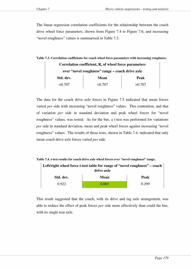
Page 179
Chapter 7 Heavy vehicle suspensions – testing and analysis
The linear regression correlation coefficients for the relationship between the coach
drive wheel force parameters, shown from Figure 7.4 to Figure 7.6, and increasing
“novel roughness” values is summarised in Table 7.3.
Table 7.3. Correlation coefficients for coach wheel force parameters with increasing roughness.
Correlation coefficient, R, of wheel force parameters
over “novel roughness” range – coach drive axle
Std. dev. Mean Peak
<0.707 <0.707 >0.707
The data for the coach drive axle forces in Figure 7.5 indicated that mean forces
varied per side with increasing “novel roughness” values. This contention, and that
of variation per side in standard deviation and peak wheel forces for “novel
roughness” values, was tested. As for the bus, a t-test was performed for variations
per side in standard deviation, mean and peak wheel forces against increasing “novel
roughness” values. The results of those tests, shown in Table 7.4, indicated that only
mean coach drive axle forces varied per side.
Table 7.4. t-test results for coach drive axle wheel forces over “novel roughness” range.
Left/right wheel force t-test table for range of “novel roughness” – coach
drive axle
Std. dev. Mean Peak
0.922 0.065 0.299
This result suggested that the coach, with its drive and tag axle arrangement, was
able to reduce the effect of peak forces per side more effectively than could the bus,
with its single rear axle.
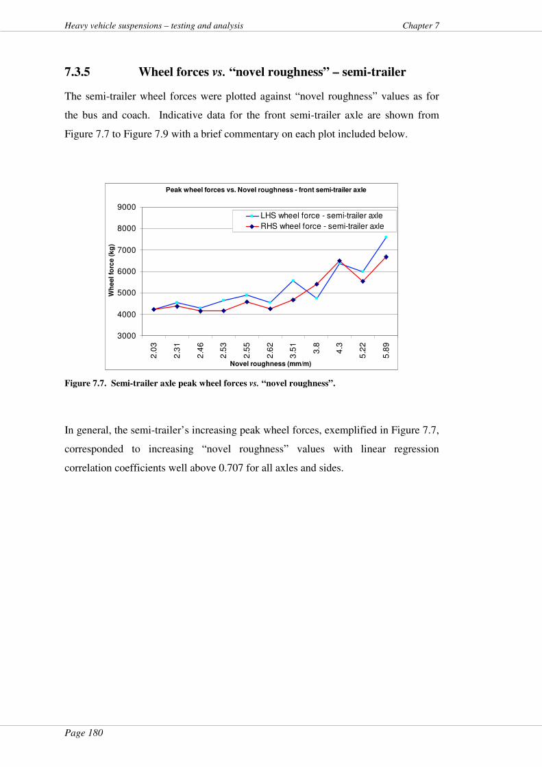
Page 180
Heavy vehicle suspensions – testing and analysis Chapter 7
7.3.5 Wheel forces vs. “novel roughness” – semi-trailer
The semi-trailer wheel forces were plotted against “novel roughness” values as for
the bus and coach. Indicative data for the front semi-trailer axle are shown from
Figure 7.7 to Figure 7.9 with a brief commentary on each plot included below.
Peak wheel forces vs. Novel roughness - front semi-trailer axle
3000
4000
5000
6000
7000
8000
9000
2.0
3
2.3
1
2.4
6
2.5
3
2.5
5
2.6
2
3.5
1
3.8
4.3
5.2
2
5.8
9
Novel roughness (mm/m)
Wh
ee
l fo
rce
(k
g)
LHS wheel force - semi-trailer axle
RHS wheel force - semi-trailer axle
Figure 7.7. Semi-trailer axle peak wheel forces vs. “novel roughness”.
In general, the semi-trailer’s increasing peak wheel forces, exemplified in Figure 7.7,
corresponded to increasing “novel roughness” values with linear regression
correlation coefficients well above 0.707 for all axles and sides.
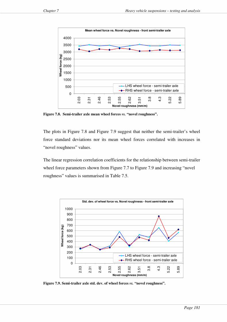
Page 181
Chapter 7 Heavy vehicle suspensions – testing and analysis
Mean wheel force vs. Novel roughness - front semi-trailer axle
0
500
1000
1500
2000
2500
3000
3500
4000
2.0
3
2.3
1
2.4
6
2.5
3
2.5
5
2.6
2
3.5
1
3.8
4.3
5.2
2
5.8
9
Novel roughness (mm/m)
Wh
ee
l fo
rce
(k
g)
LHS wheel force - semi-trailer axle
RHS wheel force - semi-trailer axle
Figure 7.8. Semi-trailer axle mean wheel forces vs. “novel roughness”.
The plots in Figure 7.8 and Figure 7.9 suggest that neither the semi-trailer’s wheel
force standard deviations nor its mean wheel forces correlated with increases in
“novel roughness” values.
The linear regression correlation coefficients for the relationship between semi-trailer
wheel force parameters shown from Figure 7.7 to Figure 7.9 and increasing “novel
roughness” values is summarised in Table 7.5.
Std. dev. of wheel force vs. Novel roughness - front semi-trailer axle
0
100
200
300
400
500
600
700
800
900
1000
2.0
3
2.3
1
2.4
6
2.5
3
2.5
5
2.6
2
3.5
1
3.8
4.3
5.2
2
5.8
9
Novel roughness (mm/m)
Wh
ee
l fo
rce
(k
g)
LHS wheel force - semi-trailer axle
RHS wheel force - semi-trailer axle
Figure 7.9. Semi-trailer axle std. dev. of wheel forces vs. “novel roughness”.
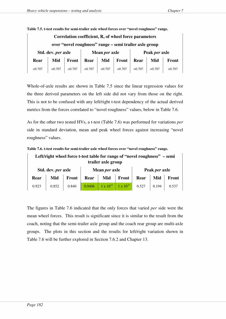
Page 182
Heavy vehicle suspensions – testing and analysis Chapter 7
Table 7.5. t-test results for semi-trailer axle wheel forces over “novel roughness” range.
Correlation coefficient, R, of wheel force parameters
over “novel roughness” range – semi trailer axle group
Std. dev. per axle Mean per axle Peak per axle
Rear Mid Front Rear Mid Front Rear Mid Front
<0.707 <0.707 <0.707 <0.707 <0.707 <0.707 >0.707 >0.707 >0.707
Whole-of-axle results are shown in Table 7.5 since the linear regression values for
the three derived parameters on the left side did not vary from those on the right.
This is not to be confused with any left/right t-test dependency of the actual derived
metrics from the forces correlated to “novel roughness” values, below in Table 7.6.
As for the other two tested HVs, a t-test (Table 7.6) was performed for variations per
side in standard deviation, mean and peak wheel forces against increasing “novel
roughness” values.
Table 7.6. t-test results for semi-trailer axle wheel forces over “novel roughness” range.
Left/right wheel force t-test table for range of “novel roughness” – semi
trailer axle group
Std. dev. per axle Mean per axle Peak per axle
Rear Mid Front Rear Mid Front Rear Mid Front
0.923 0.852 0.840 0.0406 1 x 10⁻⁴ 1 x 10⁻⁴ 0.527 0.194 0.537
The figures in Table 7.6 indicated that the only forces that varied per side were the
mean wheel forces. This result is significant since it is similar to the result from the
coach, noting that the semi-trailer axle group and the coach rear group are multi-axle
groups. The plots in this section and the results for left/right variation shown in
Table 7.6 will be further explored in Section 7.6.2 and Chapter 13.
Page 183
Chapter 7 Heavy vehicle suspensions – testing and analysis
7.4 Wheel forces left/right variation vs. speed
7.4.1 Introduction
Wheel force data during the road tests over a range of speeds were gathered in the
test programme as detailed in Section 3.2.2. Statistical analysis was performed using
a t-test to determine significance for left/right variation of wheel forces. This
analysis, unlike that undertaken in the previous section, grouped wheel force data per
test speed. The analysis below does not include the data from the 70 km/h road test.
This was because the variances in wheel force data were unequal within each speed
range. This detail ruled out a paired t-test and necessitated a heteroscedastic t-test
(Kariya & Kurata, 2004) performed for speeds of 40, 60, 80 and 90 km/h with
multiple sets of data recorded per speed. Some of this work has been published
previously, including plots of mean, standard deviation and peak wheel forces vs. test
speeds (Davis & Bunker, 2009e). Those plots have been omitted from the following
section; the interested reader is referred to them for further information. The t-test
summary table results for this data are shown from Table 7.7 to Table 7.9.
Similar to the t-test for left/right variation over the range of “novel roughness” values
in the previous section, a value for α = 0.1 with the heteroscedastic test option
(Kariya & Kurata, 2004) and a two-tailed test was used (Hamburg, 1983). Where the
results of the t-test met these criteria, they are shown from Table 7.7 to Table 7.9 in
shaded cells. A brief commentary is provided, where appropriate, on each table
below. Discussion and conclusions regarding these plots are contained in Section 7.6
and Chapter 13 including left/right variation shown from Table 7.7 to Table 7.9.
7.4.2 Left/right variation in wheel forces vs. speed
The bus wheel forces were tested for, and found dependent on, left/right position
sensitivity for some speeds as indicated in Table 7.7.
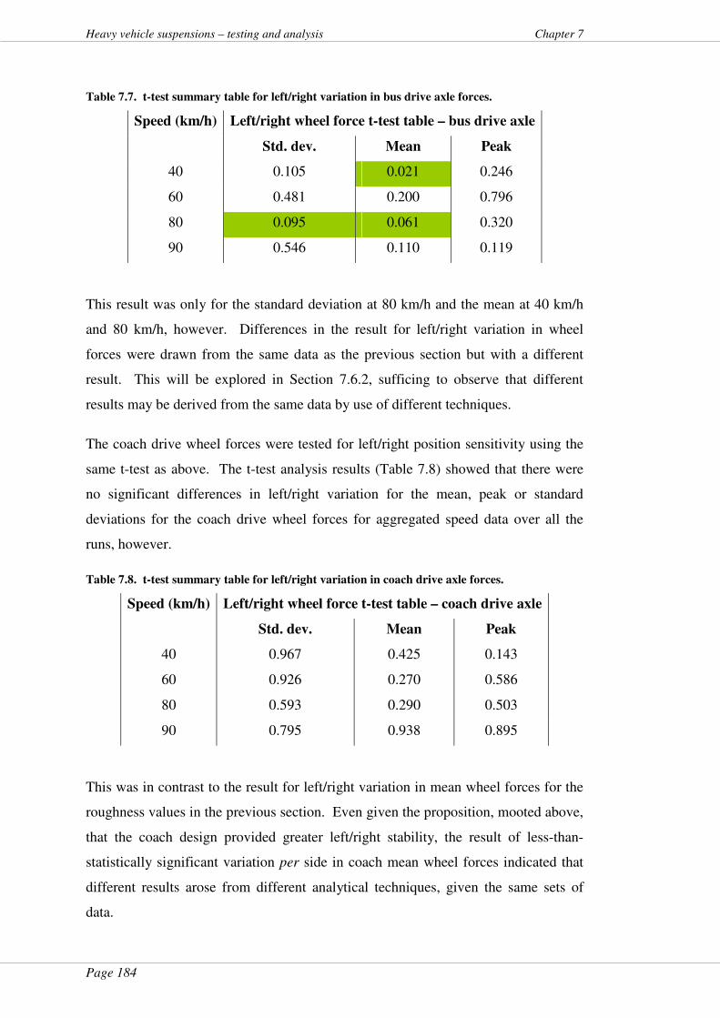
Page 184
Heavy vehicle suspensions – testing and analysis Chapter 7
Table 7.7. t-test summary table for left/right variation in bus drive axle forces.
Speed (km/h) Left/right wheel force t-test table – bus drive axle
Std. dev. Mean Peak
40 0.105 0.021 0.246
60 0.481 0.200 0.796
80 0.095 0.061 0.320
90 0.546 0.110 0.119
This result was only for the standard deviation at 80 km/h and the mean at 40 km/h
and 80 km/h, however. Differences in the result for left/right variation in wheel
forces were drawn from the same data as the previous section but with a different
result. This will be explored in Section 7.6.2, sufficing to observe that different
results may be derived from the same data by use of different techniques.
The coach drive wheel forces were tested for left/right position sensitivity using the
same t-test as above. The t-test analysis results (Table 7.8) showed that there were
no significant differences in left/right variation for the mean, peak or standard
deviations for the coach drive wheel forces for aggregated speed data over all the
runs, however.
Table 7.8. t-test summary table for left/right variation in coach drive axle forces.
Speed (km/h) Left/right wheel force t-test table – coach drive axle
Std. dev. Mean Peak
40 0.967 0.425 0.143
60 0.926 0.270 0.586
80 0.593 0.290 0.503
90 0.795 0.938 0.895
This was in contrast to the result for left/right variation in mean wheel forces for the
roughness values in the previous section. Even given the proposition, mooted above,
that the coach design provided greater left/right stability, the result of less-than-
statistically significant variation per side in coach mean wheel forces indicated that
different results arose from different analytical techniques, given the same sets of
data.
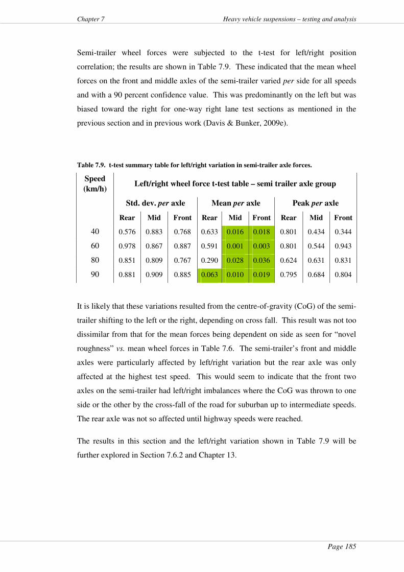
Page 185
Chapter 7 Heavy vehicle suspensions – testing and analysis
Semi-trailer wheel forces were subjected to the t-test for left/right position
correlation; the results are shown in Table 7.9. These indicated that the mean wheel
forces on the front and middle axles of the semi-trailer varied per side for all speeds
and with a 90 percent confidence value. This was predominantly on the left but was
biased toward the right for one-way right lane test sections as mentioned in the
previous section and in previous work (Davis & Bunker, 2009e).
Table 7.9. t-test summary table for left/right variation in semi-trailer axle forces.
Speed
(km/h) Left/right wheel force t-test table – semi trailer axle group
Std. dev. per axle Mean per axle Peak per axle
Rear Mid Front Rear Mid Front Rear Mid Front
40 0.576 0.883 0.768 0.633 0.016 0.018 0.801 0.434 0.344
60 0.978 0.867 0.887 0.591 0.001 0.003 0.801 0.544 0.943
80 0.851 0.809 0.767 0.290 0.028 0.036 0.624 0.631 0.831
90 0.881 0.909 0.885 0.063 0.010 0.019 0.795 0.684 0.804
It is likely that these variations resulted from the centre-of-gravity (CoG) of the semi-
trailer shifting to the left or the right, depending on cross fall. This result was not too
dissimilar from that for the mean forces being dependent on side as seen for “novel
roughness” vs. mean wheel forces in Table 7.6. The semi-trailer’s front and middle
axles were particularly affected by left/right variation but the rear axle was only
affected at the highest test speed. This would seem to indicate that the front two
axles on the semi-trailer had left/right imbalances where the CoG was thrown to one
side or the other by the cross-fall of the road for suburban up to intermediate speeds.
The rear axle was not so affected until highway speeds were reached.
The results in this section and the left/right variation shown in Table 7.9 will be
further explored in Section 7.6.2 and Chapter 13.

Page 186
Heavy vehicle suspensions – testing and analysis Chapter 7
7.4.3 Frequency of forces at the hubs and at the wheels.
A fast Fourier transform (FFT) programme was applied to the time series data from
the accelerometers at the hubs and the time series data of the wheel forces. These
FFT plots of wheel force data were derived by using Matlab FFT code developed
for the project Heavy vehicle suspensions – testing and analysis and used previously
(Davis & Bunker, 2008a, 2008e). This allowed the dominant frequencies at the axle
hub and at the wheels to be made more distinct as peaks in the spectra of both.
Indicative plots showing the predominant frequency range at the axle hubs of the test
HVs are shown from Figure 7.10 to Figure 7.12. Note that these are not necessarily
typical since some have been chosen with forces predominant on the right side, some
with left side forces predominant.
100
101
0
10
20
30
40
50
60
70FFT of LHS accelerometer signal
Frequency (Hz)
Magnitude o
f LH
S a
ccele
rom
ete
r sig
nal (a
rbitra
ry lin
ear
scale
)
10
010
10
10
20
30
40
50
60
70FFT of RHS accelerometer signal
Frequency (Hz)
Mag
nitud
e o
f R
HS
acc
ele
rom
ete
r sig
nal (a
rbitra
ry lin
ear
sc
ale
)
Figure 7.10. Frequency spectrum of drive axle hub vertical acceleration – bus, 90 km/h.
100
101
0
10
20
30
40
50
60
70FFT of LHS accelerometer signal
Frequency (Hz)
Magnitude
of
LH
S a
ccele
rom
ete
r sig
nal (a
rbitra
ry lin
ear
scale
)
100
101
0
10
20
30
40
50
60
70FFT of RHS accelerometer signal
Frequency (Hz)
Ma
gnitude o
f R
HS
ac
cele
rom
ete
r sig
na
l (a
rbitra
ry lin
ear
sc
ale
)
Figure 7.11. Frequency spectrum of drive axle hub vertical acceleration – coach, 90 km/h.
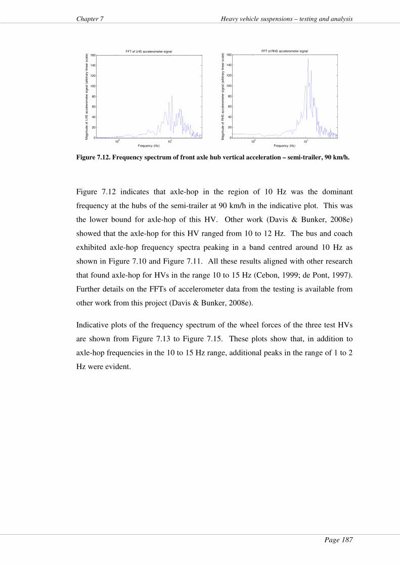
Page 187
Chapter 7 Heavy vehicle suspensions – testing and analysis
100
101
0
20
40
60
80
100
120
140
160FFT of LHS accelerometer signal
Frequency (Hz)
Magnitude o
f LH
S a
ccele
rom
ete
r sig
nal (a
rbitra
ry lin
ear
scale
)
100
101
0
20
40
60
80
100
120
140
160FFT of RHS accelerometer signal
Frequency (Hz)
Ma
gnitude o
f R
HS
ac
cele
rom
ete
r sig
na
l (a
rbitra
ry lin
ear
sc
ale
)
Figure 7.12. Frequency spectrum of front axle hub vertical acceleration – semi-trailer, 90 km/h.
Figure 7.12 indicates that axle-hop in the region of 10 Hz was the dominant
frequency at the hubs of the semi-trailer at 90 km/h in the indicative plot. This was
the lower bound for axle-hop of this HV. Other work (Davis & Bunker, 2008e)
showed that the axle-hop for this HV ranged from 10 to 12 Hz. The bus and coach
exhibited axle-hop frequency spectra peaking in a band centred around 10 Hz as
shown in Figure 7.10 and Figure 7.11. All these results aligned with other research
that found axle-hop for HVs in the range 10 to 15 Hz (Cebon, 1999; de Pont, 1997).
Further details on the FFTs of accelerometer data from the testing is available from
other work from this project (Davis & Bunker, 2008e).
Indicative plots of the frequency spectrum of the wheel forces of the three test HVs
are shown from Figure 7.13 to Figure 7.15. These plots show that, in addition to
axle-hop frequencies in the 10 to 15 Hz range, additional peaks in the range of 1 to 2
Hz were evident.
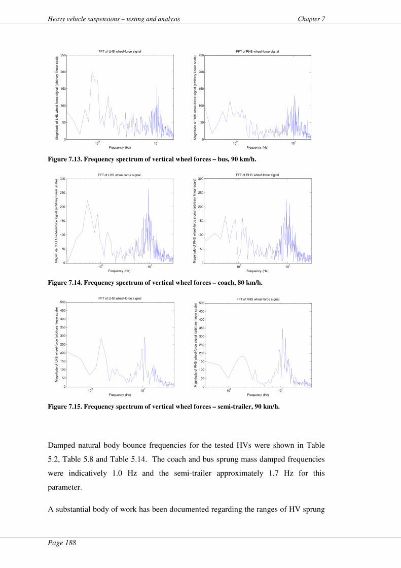
Page 188
Heavy vehicle suspensions – testing and analysis Chapter 7
100
101
0
50
100
150
200
250FFT of LHS wheel-force signal
Frequency (Hz)
Magnitude o
f LH
S w
heel-fo
rce s
ignal (a
rbitra
ry lin
ear
scale
)
100
101
0
50
100
150
200
250FFT of RHS wheel-force signal
Frequency (Hz)
Magn
itude
of
RH
S w
hee
l-fo
rce s
ignal (a
rbitra
ry lin
ear
scale
)
Figure 7.13. Frequency spectrum of vertical wheel forces – bus, 90 km/h.
100
101
0
50
100
150
200
250
300FFT of LHS wheel-force signal
Frequency (Hz)
Magnitude o
f LH
S w
heel-fo
rce s
ignal (a
rbitra
ry lin
ear
scale
)
100
101
0
50
100
150
200
250
300FFT of RHS wheel-force signal
Frequency (Hz)
Magnitude o
f R
HS
wheel-fo
rce s
ignal (a
rbitra
ry lin
ear
scale
)
Figure 7.14. Frequency spectrum of vertical wheel forces – coach, 80 km/h.
100
101
0
50
100
150
200
250
300
350
400
450
500FFT of LHS wheel-force signal
Frequency (Hz)
Magnitude o
f LH
S w
heel-fo
rce (
arb
itra
ry lin
ear
scale
)
100
101
0
50
100
150
200
250
300
350
400
450
500FFT of RHS wheel-force signal
Frequency (Hz)
Mag
nitude o
f R
HS
wheel-
forc
e s
ignal (a
rbitra
ry l
inear
scale
)
Figure 7.15. Frequency spectrum of vertical wheel forces – semi-trailer, 90 km/h.
Damped natural body bounce frequencies for the tested HVs were shown in Table
5.2, Table 5.8 and Table 5.14. The coach and bus sprung mass damped frequencies
were indicatively 1.0 Hz and the semi-trailer approximately 1.7 Hz for this
parameter.
A substantial body of work has been documented regarding the ranges of HV sprung
Page 189
Chapter 7 Heavy vehicle suspensions – testing and analysis
mass (body bounce) and axle-hop (unsprung mass) frequencies. Cebon (1987), Cole
and Cebon (1994) and Chatti and Lee (2002), among many others, have noted sprung
mass damped natural frequencies of HVs in the 1 to 4 Hz range with unsprung mass
damped natural frequencies in the 10 to 15 Hz range.
The twin peaks in the measured wheel force frequency spectra were indicative of a
combination of body bounce at these frequencies and a component at approximately
10 Hz from axle-hop. This indicated that forces from body bounce were being added
to axle-hop forces to produce the total wheel forces. Figure 7.16 shows an indicative
method for visualising this concept. This example is illustrative of wheel forces
derived from the testing being the sum of sprung and unsprung mass signals
containing the peaks in damped natural frequencies of the sprung and unsprung
masses.
The damped natural frequency of the sprung mass in Figure 7.16 is indicated by a
peak in the frequency spectrum amplitude of the signals measured at the air pressure
transducers during the testing detailed in Section 3.2. Similarly, the axle-hop
frequency is indicated by a peak in the amplitude of the FFT spectrum from the
indicative accelerometer signals shown.

Page 190
Heavy vehicle suspensions – testing and analysis Chapter 7
Figure 7.16. Indicating that peak in the vertical wheel force spectrum may be seen as an
addition of damped and undamped natural frequencies.
Body bounce
Axle-hop
Page 191
Chapter 7 Heavy vehicle suspensions – testing and analysis
These results will be used in Section 7.4.4 to expand on spatial repetition of wheel
forces.
7.4.4 Suspension wavelength and spatial repetition
The axle-hop and body bounce frequencies, shown from Figure 7.13 to Figure 7.15,
were translated back into wavelengths. Since frequency may be found as the inverse
of the signal period (Equation 4.14), wavelength was derived from the test speed and
the fundamental relationship between speed and distance as follows:
tvd ×=
Equation 7.3
where:
v = speed in metres.s-1;
d = distance in m; and
t = time in s.
Substituting 1/f for t, from first principles, the distance between successive peaks in
the wheel forces may be derived:
d = v/f
Equation 7.4
Applying Equation 7.4 to the frequency data sets from this project (Davis & Bunker,
2008e), the tested HVs’ suspension wavelengths were derived after examining the
predominant axle-hop and body bounce frequencies and corresponding test speeds.
These are summarised in Table 7.10.
The "spatial repetition" approach has been discussed in Section 2.4 (Cebon, 1987;
Collop & Cebon, 2002; Potter, Cebon, & Cole, 1997; Potter, Cebon, Cole et al.,
1995). How this concept relates to the data derived in Table 7.10 will be expanded
later in this chapter. For the purposes of presentation of derived data, however,
consideration may be given to peak loadings from the HVs tested for this project.
Note that the bold figures in Table 7.10 are for the predominant frequencies and
wavelength distances at the corresponding speed; i.e. body bounce predominated at
60 km/h but both body bounce and axle-hop were approximately equal magnitude at
80 km/h and 90 km/h (Davis & Bunker, 2008e).
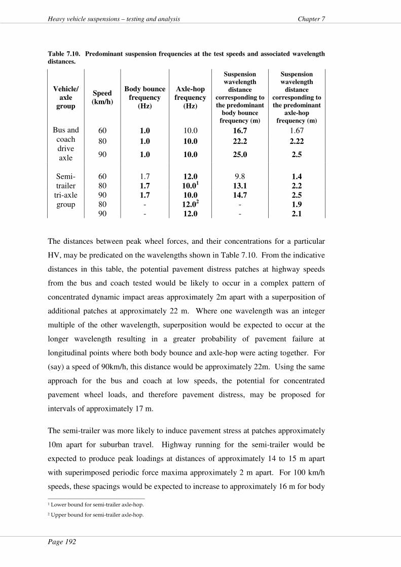
Page 192
Heavy vehicle suspensions – testing and analysis Chapter 7
Table 7.10. Predominant suspension frequencies at the test speeds and associated wavelength
distances.
Vehicle/
axle
group
Speed
(km/h)
Body bounce
frequency
(Hz)
Axle-hop
frequency
(Hz)
Suspension
wavelength
distance
corresponding to
the predominant
body bounce
frequency (m)
Suspension
wavelength
distance
corresponding to
the predominant
axle-hop
frequency (m)
60 1.0 10.0 16.7 1.67
80 1.0 10.0 22.2 2.22
Bus and coach drive axle 90 1.0 10.0 25.0 2.5
60
1.7
12.0
9.8
1.4 80 1.7 10.0
1 13.1 2.2
90 1.7 10.0 14.7 2.5 80 - 12.0
2 - 1.9
Semi-trailer
tri-axle group
90 - 12.0 - 2.1
The distances between peak wheel forces, and their concentrations for a particular
HV, may be predicated on the wavelengths shown in Table 7.10. From the indicative
distances in this table, the potential pavement distress patches at highway speeds
from the bus and coach tested would be likely to occur in a complex pattern of
concentrated dynamic impact areas approximately 2m apart with a superposition of
additional patches at approximately 22 m. Where one wavelength was an integer
multiple of the other wavelength, superposition would be expected to occur at the
longer wavelength resulting in a greater probability of pavement failure at
longitudinal points where both body bounce and axle-hop were acting together. For
(say) a speed of 90km/h, this distance would be approximately 22m. Using the same
approach for the bus and coach at low speeds, the potential for concentrated
pavement wheel loads, and therefore pavement distress, may be proposed for
intervals of approximately 17 m.
The semi-trailer was more likely to induce pavement stress at patches approximately
10m apart for suburban travel. Highway running for the semi-trailer would be
expected to produce peak loadings at distances of approximately 14 to 15 m apart
with superimposed periodic force maxima approximately 2 m apart. For 100 km/h
speeds, these spacings would be expected to increase to approximately 16 m for body
1 Lower bound for semi-trailer axle-hop.
2 Upper bound for semi-trailer axle-hop.
Page 193
Chapter 7 Heavy vehicle suspensions – testing and analysis
bounce and range from 2.3 m to 2.7 m for axle-hop (Equation 7.4 and Table 7.10).
Superposition would suggest that, where the longer spacings coincided with the
spatial repetition of axle-hop forces, greater pavement distress would occur as a
patch.
7.5 In-service heavy vehicle suspension testing -
roller bed
7.5.1 Introduction
Objective 3 of this project was to develop two low-cost HV suspension tests. The
“pipe test” results have been described and analysed (Chapter 6). For the second low
cost test, as detailed in Section 3.3, a wheel within a HV suspension group was
vibrated on a roller bed modified from a HV brake testing unit. The forces at the
roller for a control case of new dampers were compared with two test cases for worn
dampers. The first test case was for a damper worn to the point where tyre wear was
apparent due to flat spots on the tyre; the second test case was for no damper. The
peak-to-peak values (i.e. the dynamic range) of wheel force signals were derived for
these cases. This was in line with the description in Section 3.3 for combinations of
the three cases of shock absorber health, two test speeds and rollers with machined
areas of 2 mm and 4 mm radial depths.
7.5.2 Peak dynamic forces
As mentioned in Section 3.3, the two test speeds were designed to envelop, but just
exceed, body bounce (1.7 Hz) and axle-hop (12 Hz) frequencies for this semi-trailer.
The dynamic range concept is illustrated in Figure 7.17.
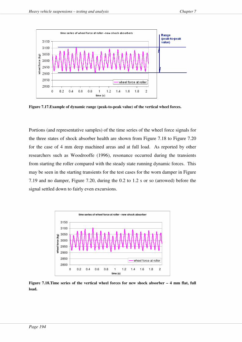
Page 194
Heavy vehicle suspensions – testing and analysis Chapter 7
Figure 7.17.Example of dynamic range (peak-to-peak value) of the vertical wheel forces.
Portions (and representative samples) of the time series of the wheel force signals for
the three states of shock absorber health are shown from Figure 7.18 to Figure 7.20
for the case of 4 mm deep machined areas and at full load. As reported by other
researchers such as Woodrooffe (1996), resonance occurred during the transients
from starting the roller compared with the steady state running dynamic forces. This
may be seen in the starting transients for the test cases for the worn damper in Figure
7.19 and no damper, Figure 7.20, during the 0.2 to 1.2 s or so (arrowed) before the
signal settled down to fairly even excursions.
time series of wheel force at roller - new shock absorber
2800
2850
2900
2950
3000
3050
3100
3150
0 0.2 0.4 0.6 0.8 1 1.2 1.4 1.6 1.8 2
time (s)
wh
ee
l fo
rce (
kg
)
wheel force at roller
Figure 7.18.Time series of the vertical wheel forces for new shock absorber – 4 mm flat, full
load.
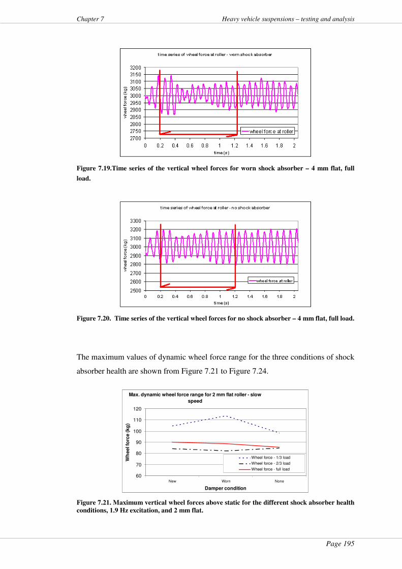
Page 195
Chapter 7 Heavy vehicle suspensions – testing and analysis
Figure 7.19.Time series of the vertical wheel forces for worn shock absorber – 4 mm flat, full
load.
Figure 7.20. Time series of the vertical wheel forces for no shock absorber – 4 mm flat, full load.
The maximum values of dynamic wheel force range for the three conditions of shock
absorber health are shown from Figure 7.21 to Figure 7.24.
Max. dynamic wheel force range for 2 mm flat roller - slow
speed
60
70
80
90
100
110
120
New Worn None
Damper condition
Wh
ee
l fo
rce
(k
g)
Wheel force - 1/3 load
Wheel force - 2/3 load
Wheel force - full load
Figure 7.21. Maximum vertical wheel forces above static for the different shock absorber health
conditions, 1.9 Hz excitation, and 2 mm flat.
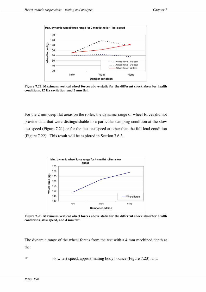
Page 196
Heavy vehicle suspensions – testing and analysis Chapter 7
Max. dynamic wheel force range for 2 mm flat roller - fast speed
20
40
60
80
100
120
140
160
New Worn None
Damper condition
Wh
ee
l fo
rce
(k
g)
Wheel force - 1/3 load
Wheel force - 2/3 load
Wheel force - full load
Figure 7.22. Maximum vertical wheel forces above static for the different shock absorber health
conditions, 12 Hz excitation, and 2 mm flat.
For the 2 mm deep flat areas on the roller, the dynamic range of wheel forces did not
provide data that were distinguishable to a particular damping condition at the slow
test speed (Figure 7.21) or for the fast test speed at other than the full load condition
(Figure 7.22). This result will be explored in Section 7.6.3.
Max. dynamic wheel force range for 4 mm flat roller - slow
speed
140
145
150
155
160
165
170
175
New Worn None
Damper condition
Wh
ee
l fo
rce
(k
g)
Wheel force
Figure 7.23. Maximum vertical wheel forces above static for the different shock absorber health
conditions, slow speed, and 4 mm flat.
The dynamic range of the wheel forces from the test with a 4 mm machined depth at
the:
� slow test speed, approximating body bounce (Figure 7.23); and
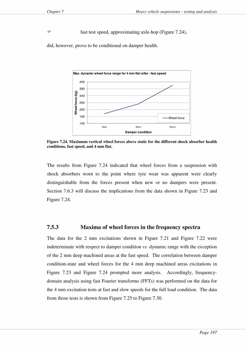
Page 197
Chapter 7 Heavy vehicle suspensions – testing and analysis
� fast test speed, approximating axle-hop (Figure 7.24),
did, however, prove to be conditional on damper health.
Max. dynamic wheel force range for 4 mm flat roller - fast speed
140
190
240
290
340
390
440
New Worn None
Damper condition
Wh
ee
l fo
rce (
kg
)
Wheel force
Figure 7.24. Maximum vertical wheel forces above static for the different shock absorber health
conditions, fast speed, and 4 mm flat.
The results from Figure 7.24 indicated that wheel forces from a suspension with
shock absorbers worn to the point where tyre wear was apparent were clearly
distinguishable from the forces present when new or no dampers were present.
Section 7.6.3 will discuss the implications from the data shown in Figure 7.23 and
Figure 7.24.
7.5.3 Maxima of wheel forces in the frequency spectra
The data for the 2 mm excitations shown in Figure 7.21 and Figure 7.22 were
indeterminate with respect to damper condition vs. dynamic range with the exception
of the 2 mm deep machined areas at the fast speed. The correlation between damper
condition-state and wheel forces for the 4 mm deep machined areas excitations in
Figure 7.23 and Figure 7.24 prompted more analysis. Accordingly, frequency-
domain analysis using fast Fourier transforms (FFTs) was performed on the data for
the 4 mm excitation tests at fast and slow speeds for the full load condition. The data
from those tests is shown from Figure 7.25 to Figure 7.30.
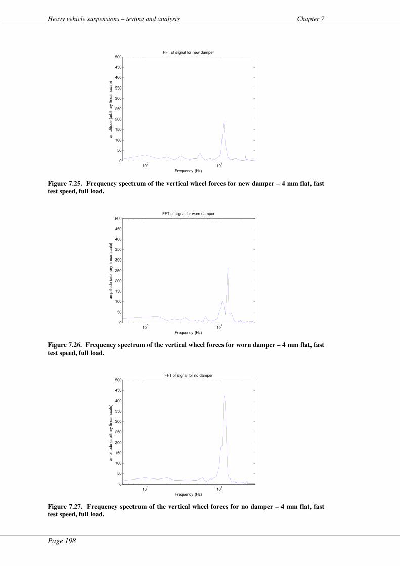
Page 198
Heavy vehicle suspensions – testing and analysis Chapter 7
100
101
0
50
100
150
200
250
300
350
400
450
500FFT of signal for new damper
Frequency (Hz)
am
plit
ude (
arb
itra
ry lin
ear
scale
)
Figure 7.25. Frequency spectrum of the vertical wheel forces for new damper – 4 mm flat, fast
test speed, full load.
100
101
0
50
100
150
200
250
300
350
400
450
500FFT of signal for worn damper
Frequency (Hz)
am
plit
ude (
arb
itra
ry lin
ear
scale
)
Figure 7.26. Frequency spectrum of the vertical wheel forces for worn damper – 4 mm flat, fast
test speed, full load.
100
101
0
50
100
150
200
250
300
350
400
450
500FFT of signal for no damper
Frequency (Hz)
am
plit
ude (
arb
itra
ry lin
ear
scale
)
Figure 7.27. Frequency spectrum of the vertical wheel forces for no damper – 4 mm flat, fast
test speed, full load.
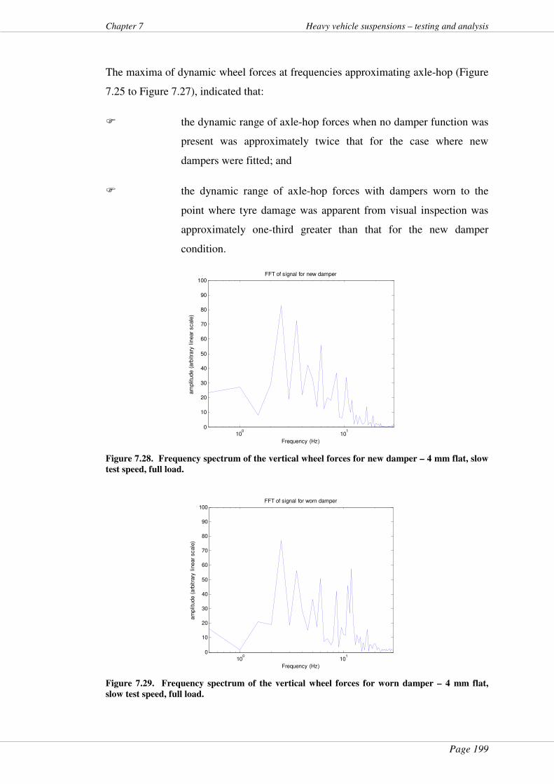
Page 199
Chapter 7 Heavy vehicle suspensions – testing and analysis
The maxima of dynamic wheel forces at frequencies approximating axle-hop (Figure
7.25 to Figure 7.27), indicated that:
� the dynamic range of axle-hop forces when no damper function was
present was approximately twice that for the case where new
dampers were fitted; and
� the dynamic range of axle-hop forces with dampers worn to the
point where tyre damage was apparent from visual inspection was
approximately one-third greater than that for the new damper
condition.
100
101
0
10
20
30
40
50
60
70
80
90
100FFT of signal for new damper
Frequency (Hz)
am
plit
ude (
arb
itra
ry lin
ear
scale
)
Figure 7.28. Frequency spectrum of the vertical wheel forces for new damper – 4 mm flat, slow
test speed, full load.
100
101
0
10
20
30
40
50
60
70
80
90
100FFT of signal for worn damper
Frequency (Hz)
am
plit
ude (
arb
itra
ry lin
ear
scale
)
Figure 7.29. Frequency spectrum of the vertical wheel forces for worn damper – 4 mm flat,
slow test speed, full load.
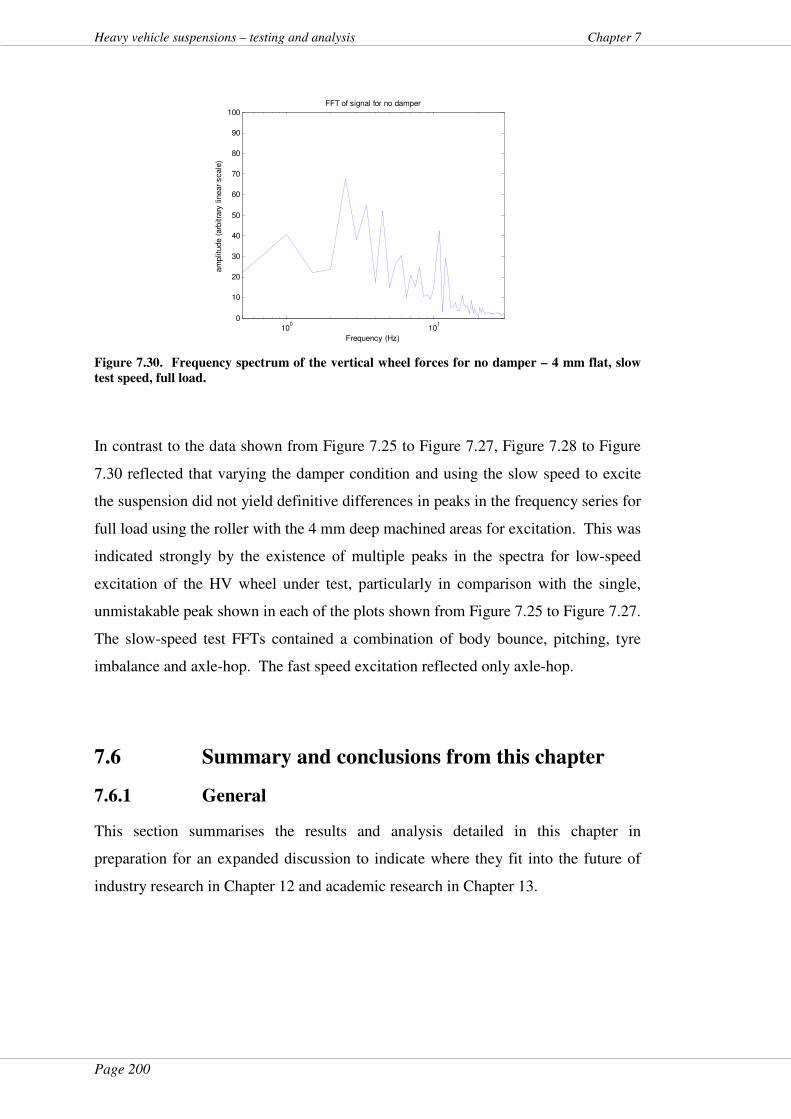
Page 200
Heavy vehicle suspensions – testing and analysis Chapter 7
100
101
0
10
20
30
40
50
60
70
80
90
100FFT of signal for no damper
Frequency (Hz)
am
plit
ude (
arb
itra
ry lin
ear
scale
)
Figure 7.30. Frequency spectrum of the vertical wheel forces for no damper – 4 mm flat, slow
test speed, full load.
In contrast to the data shown from Figure 7.25 to Figure 7.27, Figure 7.28 to Figure
7.30 reflected that varying the damper condition and using the slow speed to excite
the suspension did not yield definitive differences in peaks in the frequency series for
full load using the roller with the 4 mm deep machined areas for excitation. This was
indicated strongly by the existence of multiple peaks in the spectra for low-speed
excitation of the HV wheel under test, particularly in comparison with the single,
unmistakable peak shown in each of the plots shown from Figure 7.25 to Figure 7.27.
The slow-speed test FFTs contained a combination of body bounce, pitching, tyre
imbalance and axle-hop. The fast speed excitation reflected only axle-hop.
7.6 Summary and conclusions from this chapter
7.6.1 General
This section summarises the results and analysis detailed in this chapter in
preparation for an expanded discussion to indicate where they fit into the future of
industry research in Chapter 12 and academic research in Chapter 13.
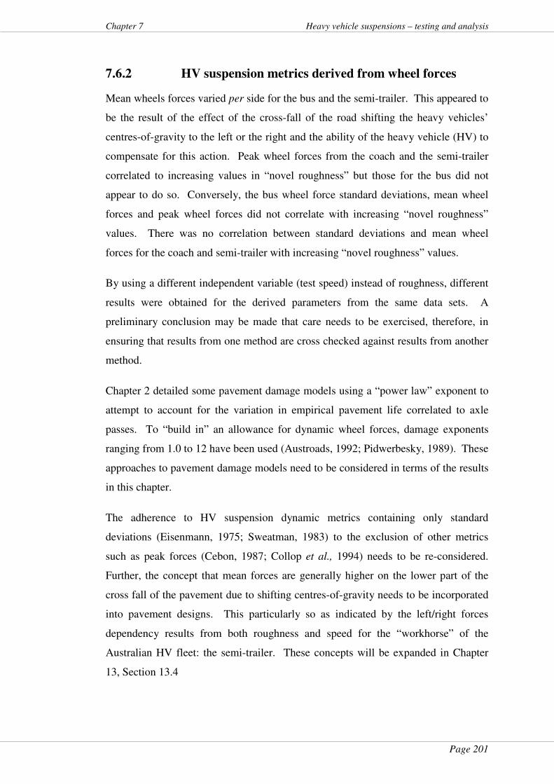
Page 201
Chapter 7 Heavy vehicle suspensions – testing and analysis
7.6.2 HV suspension metrics derived from wheel forces
Mean wheels forces varied per side for the bus and the semi-trailer. This appeared to
be the result of the effect of the cross-fall of the road shifting the heavy vehicles’
centres-of-gravity to the left or the right and the ability of the heavy vehicle (HV) to
compensate for this action. Peak wheel forces from the coach and the semi-trailer
correlated to increasing values in “novel roughness” but those for the bus did not
appear to do so. Conversely, the bus wheel force standard deviations, mean wheel
forces and peak wheel forces did not correlate with increasing “novel roughness”
values. There was no correlation between standard deviations and mean wheel
forces for the coach and semi-trailer with increasing “novel roughness” values.
By using a different independent variable (test speed) instead of roughness, different
results were obtained for the derived parameters from the same data sets. A
preliminary conclusion may be made that care needs to be exercised, therefore, in
ensuring that results from one method are cross checked against results from another
method.
Chapter 2 detailed some pavement damage models using a “power law” exponent to
attempt to account for the variation in empirical pavement life correlated to axle
passes. To “build in” an allowance for dynamic wheel forces, damage exponents
ranging from 1.0 to 12 have been used (Austroads, 1992; Pidwerbesky, 1989). These
approaches to pavement damage models need to be considered in terms of the results
in this chapter.
The adherence to HV suspension dynamic metrics containing only standard
deviations (Eisenmann, 1975; Sweatman, 1983) to the exclusion of other metrics
such as peak forces (Cebon, 1987; Collop et al., 1994) needs to be re-considered.
Further, the concept that mean forces are generally higher on the lower part of the
cross fall of the pavement due to shifting centres-of-gravity needs to be incorporated
into pavement designs. This particularly so as indicated by the left/right forces
dependency results from both roughness and speed for the “workhorse” of the
Australian HV fleet: the semi-trailer. These concepts will be expanded in Chapter
13, Section 13.4
Page 202
Heavy vehicle suspensions – testing and analysis Chapter 7
7.6.3 Regarding the dynamic range for different damper
conditions
The experimental design was framed to determine if the damper condition was
apparent from measuring the dynamic range of wheel force signals. By exciting one
side and leaving the other side free to vibrate, axle roll was generated. This was
considered in terms of how the auxiliary roll stiffness of the axle would have affected
the results. The only variable that was altered between tests was the damping
characteristic of the shock absorber. The axle auxiliary roll stiffness leading to the
phenomenon of axle roll was common to all tests. Accordingly, any influence that
axle roll had on the measured net dynamic forces from the HV wheel for each case of
damping characteristics was present in the results of all tests. Since only relative
values of wheel force dynamic ranges were considered, the axle roll component for
individual results therefore cancelled.
Damper conditions were varied from new to no damping. With 4 mm deep
machined areas on the roller, the overall dynamic wheel forces above static were
approximately doubled when comparing the control case of new shock absorber of
vs. the test case of no shock absorbers. Further, with dampers worn to the point
where they were causing tyre wear, peak dynamic forces were approximately 30
percent greater than for the case of the new damper.
The frequency and time series analysis of the data for 2 mm deep machined areas on
the roller at either 1.9 Hz or 12 Hz did not yield definitive conclusions regarding
damper health. Further, the frequency domain analysis of the data from the 4 mm
deep machined areas at 1.9 Hz did not prove conclusive with respect to damper
condition. However, as a “proof-of-concept”, both the frequency and time domain
analysis showed that damper condition could be detected using the test rig at axle-
hop frequencies with 4 mm deep machined areas on the roller. Accordingly, these
results will need to be considered in any future designs for in-service testing for HV
suspensions.
Development of in-service testing of HV suspensions, should the current National
Transport Commission project consider a method similar to that detailed in this
project, will need to ensure that sufficient amplitude is imparted to the HV wheel for
meaningful differentiation of damper health to occur.
Page 203
Chapter 7 Heavy vehicle suspensions – testing and analysis
The results also allowed a judgement to be made regarding the additional damage
that worn dampers contribute to the community cost of providing the transport
network. This will be explored in Chapter 12, Section 12.4.2.
7.6.4 Regarding the use of tyre wear as an indicator of
damper health
Using tyre wear as an indicator that suspension dampers are worn is not an indicator
that results in timely shock absorber replacement. The results of in-service
compliance testing by Blanksby et al., (2006) showed that HVs without noticeable
tyre wear fell outside the “road friendly” criteria for damping ratio in over 50 percent
of the tested population. This issue will be further explored in Chapter 12, Section
12.4.1.
7.7 Chapter close
7.7.1 General
Chapter 3 described methodologies that resulted in large data sets for wheel force
data. Some of those data sets have been analysed in this chapter for wheel forces
during the on-road tests. A “novel roughness metric” or “novel roughness” measure
was developed. Application of this “novel roughness” parameter led to results and
preliminary conclusions regarding how some wheel force metrics, such as peak
values and standard deviations to name two, are related to left/right side bias and
“novel roughness”. Analysis of left/right differences in wheel forces was also
presented for speed ranges as recorded and described in Chapter 3.
The “novel roughness” measure will be used in Chapter 10 to explore whether larger
longitudinal air lines alter air suspension behaviour. Chapter 11 will explore in-
service HV suspension testing informed by the results of the roller bed tests analysed
in this chapter. Further, the issue of tyre wear as an indicator that suspension
dampers are worn will be further explored in Chapter 12, Section 12.4.1, supported
by the analysis detailed herein. That differing levels of wheel force were evident for
different levels of damper health was shown in this chapter. These data will be used
Page 204
Heavy vehicle suspensions – testing and analysis Chapter 7
in an indicative exercise regarding the community cost of poor damper maintenance
in Chapter 12, Section 12.4.2. Future research directions will be expanded in
Chapter 13, Section 13.3 as informed by the approaches shown above.
Links where this chapter informs other chapters of this thesis are shown in Figure
1.4.
Page 205
Chapter 8 Heavy vehicle suspensions – testing and analysis
8 On-board mass system characterisation
8.1 About this chapter
This chapter summarises the applicable results of the non-tamper testing
(methodology as documented in Section 3.4) conducted as part of the on-board mass
(OBM) system accuracy and tamper-evidence activity to meet Objective 4.
The OBM testing was overseen by Transport Certification Australia (TCA) as lead
agency. Various data from that test programme contributed to the project “Heavy
vehicle suspensions – testing and analysis”.
8.2 Introduction
OBM systems were tested as part of this research programme. Those test procedures
were covered in Section 3.4 with the rationale for the test programme covered in
Section 1.5. The on-board mass (OBM) systems presented to the testing team were
tested in their “as offered” condition (Section 3.4). Sometimes this condition was
without particular prior preparation, save for calibration, or without the OBM
systems installed on vehicles selected with a great deal of prior notice. The test
team’s original view was that the supplier of the OBM system under test would
borrow a heavy vehicle (HV) from their client (Davis et al., 2008b) and this was the
case for majority of the HVs and OBM systems tested. This arrangement allowed
testing to proceed on HVs and OBM systems in regular service. In some cases,
however, the prevailing economic situation during the testing precluded the use of
working HVs since they could not be freed from normal service to allow the testing
to proceed. In these instances, the tested HVs were hire units with OBM systems
installed and calibrated immediately prior to the testing.
The test plans under which the testing was carried out contained elements developed
to determine the accuracy and tamper evidence of contemporary, commercially-
available OBM units in Australia (Davis et al., 2008a, 2008b). From the data
recorded during the testing, evidence was collected that allowed determination of
accuracy and tamper-evidence of those systems. This chapter provides:
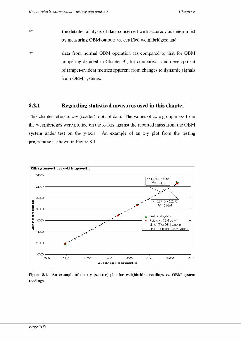
Page 206
Heavy vehicle suspensions – testing and analysis Chapter 8
� the detailed analysis of data concerned with accuracy as determined
by measuring OBM outputs vs. certified weighbridges; and
� data from normal OBM operation (as compared to that for OBM
tampering detailed in Chapter 9), for comparison and development
of tamper-evident metrics apparent from changes to dynamic signals
from OBM systems.
8.2.1 Regarding statistical measures used in this chapter
This chapter refers to x-y (scatter) plots of data. The values of axle group mass from
the weighbridges were plotted on the x-axis against the reported mass from the OBM
system under test on the y-axis. An example of an x-y plot from the testing
programme is shown in Figure 8.1.
Figure 8.1. An example of an x-y (scatter) plot for weighbridge readings vs. OBM system
readings.
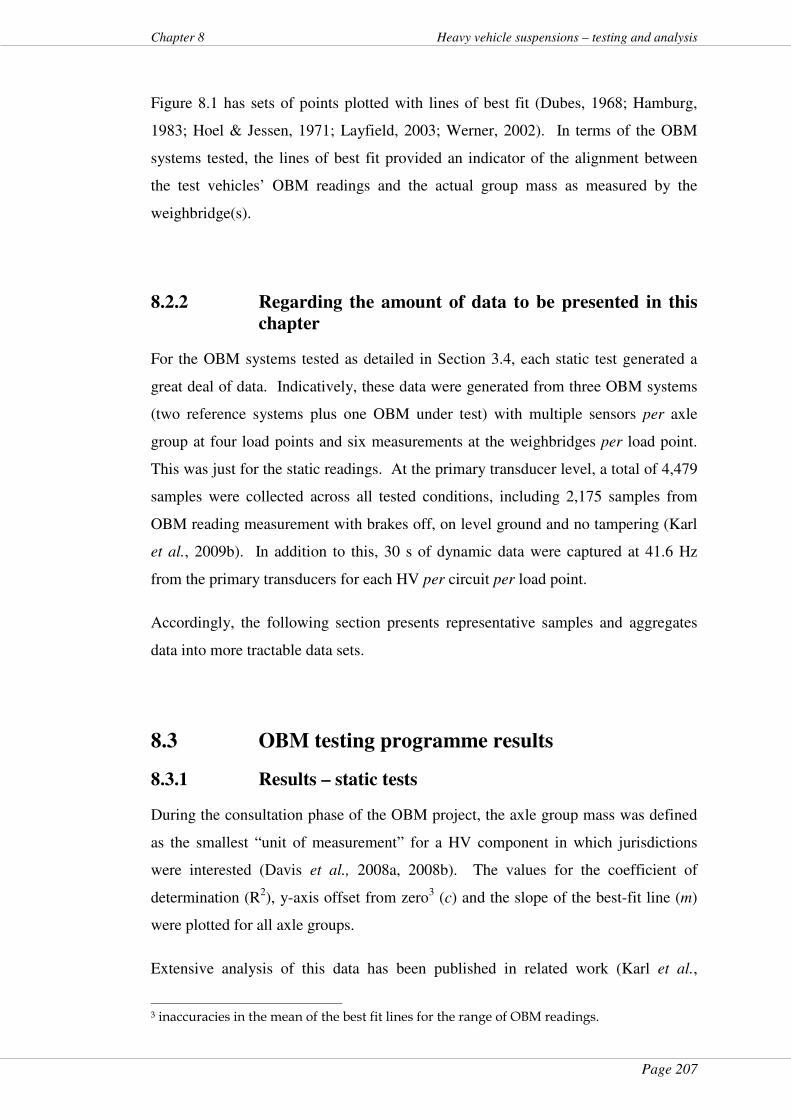
Page 207
Chapter 8 Heavy vehicle suspensions – testing and analysis
Figure 8.1 has sets of points plotted with lines of best fit (Dubes, 1968; Hamburg,
1983; Hoel & Jessen, 1971; Layfield, 2003; Werner, 2002). In terms of the OBM
systems tested, the lines of best fit provided an indicator of the alignment between
the test vehicles’ OBM readings and the actual group mass as measured by the
weighbridge(s).
8.2.2 Regarding the amount of data to be presented in this
chapter
For the OBM systems tested as detailed in Section 3.4, each static test generated a
great deal of data. Indicatively, these data were generated from three OBM systems
(two reference systems plus one OBM under test) with multiple sensors per axle
group at four load points and six measurements at the weighbridges per load point.
This was just for the static readings. At the primary transducer level, a total of 4,479
samples were collected across all tested conditions, including 2,175 samples from
OBM reading measurement with brakes off, on level ground and no tampering (Karl
et al., 2009b). In addition to this, 30 s of dynamic data were captured at 41.6 Hz
from the primary transducers for each HV per circuit per load point.
Accordingly, the following section presents representative samples and aggregates
data into more tractable data sets.
8.3 OBM testing programme results
8.3.1 Results – static tests
During the consultation phase of the OBM project, the axle group mass was defined
as the smallest “unit of measurement” for a HV component in which jurisdictions
were interested (Davis et al., 2008a, 2008b). The values for the coefficient of
determination (R2), y-axis offset from zero3 (c) and the slope of the best-fit line (m)
were plotted for all axle groups.
Extensive analysis of this data has been published in related work (Karl et al.,
3 inaccuracies in the mean of the best fit lines for the range of OBM readings.
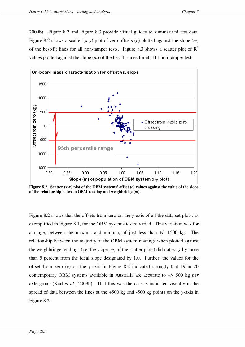
Page 208
Heavy vehicle suspensions – testing and analysis Chapter 8
2009b). Figure 8.2 and Figure 8.3 provide visual guides to summarised test data.
Figure 8.2 shows a scatter (x-y) plot of zero offsets (c) plotted against the slope (m)
of the best-fit lines for all non-tamper tests. Figure 8.3 shows a scatter plot of R2
values plotted against the slope (m) of the best-fit lines for all 111 non-tamper tests.
Figure 8.2. Scatter (x-y) plot of the OBM systems’ offset (c) values against the value of the slope
of the relationship between OBM reading and weighbridge (m).
Figure 8.2 shows that the offsets from zero on the y-axis of all the data set plots, as
exemplified in Figure 8.1, for the OBM systems tested varied. This variation was for
a range, between the maxima and minima, of just less than +/- 1500 kg. The
relationship between the majority of the OBM system readings when plotted against
the weighbridge readings (i.e. the slope, m, of the scatter plots) did not vary by more
than 5 percent from the ideal slope designated by 1.0. Further, the values for the
offset from zero (c) on the y-axis in Figure 8.2 indicated strongly that 19 in 20
contemporary OBM systems available in Australia are accurate to +/- 500 kg per
axle group (Karl et al., 2009b). That this was the case is indicated visually in the
spread of data between the lines at the +500 kg and -500 kg points on the y-axis in
Figure 8.2.
Page 209
Chapter 8 Heavy vehicle suspensions – testing and analysis
Figure 8.3. Scatter (x-y) plot of the OBM systems’ R
2 values against the value of the slope of the
relationship between OBM reading and weighbridge (m).
As a visual guide, the cluster of R2 values in Figure 8.3 indicates that all OBM
individual system tests (save for three) had R2 values in the range 0.995 to 1.0; other
analysis (Karl et al., 2009b) provides more detail. Further, as a visual account, the
coefficient of determination (R2) values for all OBM system tested were very closely
clustered around 1.0. This spread of R2 values represented a total variation in
linearity of 0.5 percent when the three outliers were removed. This was judged a
very good result for jurisdictions and the OBM industry as will be discussed later in
this chapter. How these results will influence OBM, if implemented in the future,
and implications for the OBM industry and jurisdictions will be expanded later in
this chapter and in Chapter 12, Section 12.5.
8.3.2 Results – analysis of dynamic data for non-tamper
events
Section 3.4 detailed the testing procedures. In brief, as they relate to dynamic data
gathering, the test HVs were driven around a convenient test circuit of a typically
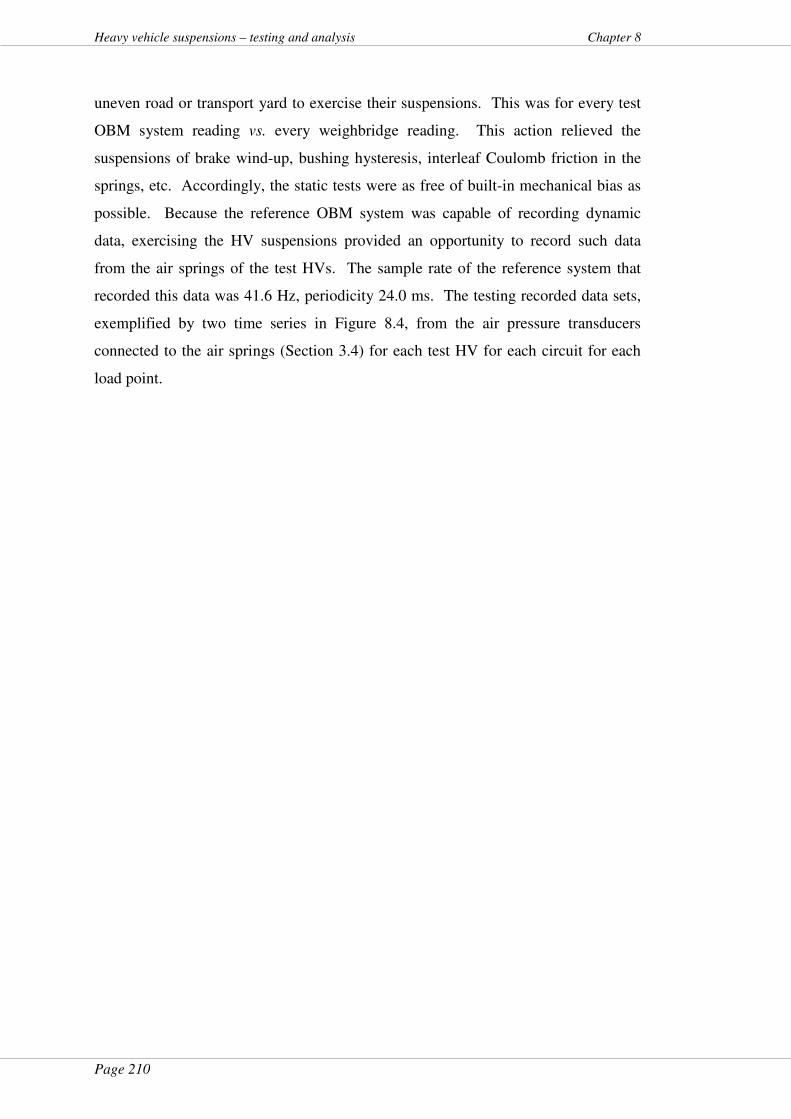
Page 210
Heavy vehicle suspensions – testing and analysis Chapter 8
uneven road or transport yard to exercise their suspensions. This was for every test
OBM system reading vs. every weighbridge reading. This action relieved the
suspensions of brake wind-up, bushing hysteresis, interleaf Coulomb friction in the
springs, etc. Accordingly, the static tests were as free of built-in mechanical bias as
possible. Because the reference OBM system was capable of recording dynamic
data, exercising the HV suspensions provided an opportunity to record such data
from the air springs of the test HVs. The sample rate of the reference system that
recorded this data was 41.6 Hz, periodicity 24.0 ms. The testing recorded data sets,
exemplified by two time series in Figure 8.4, from the air pressure transducers
connected to the air springs (Section 3.4) for each test HV for each circuit for each
load point.
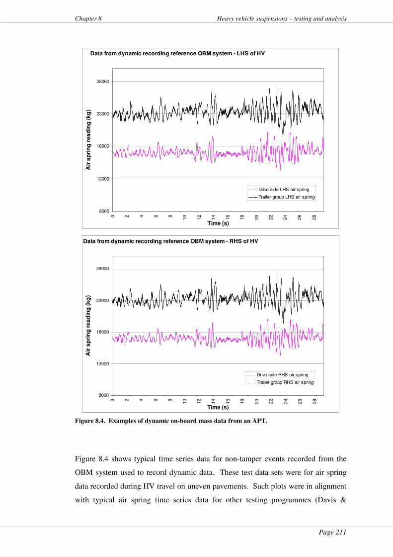
Page 211
Chapter 8 Heavy vehicle suspensions – testing and analysis
Data from dynamic recording reference OBM system - LHS of HV
8000
13000
18000
23000
28000
0 2 4 6 8
10
12
14
16
18
20
22
24
26
28
Time (s)
Air
sp
rin
g r
ead
ing
(kg
)
Drive axle LHS air spring
Trailer group LHS air spring
Data from dynamic recording reference OBM system - RHS of HV
8000
13000
18000
23000
28000
0 2 4 6 8
10
12
14
16
18
20
22
24
26
28
Time (s)
Air
sp
rin
g r
ead
ing
(kg
)
Drive axle RHS air spring
Trailer group RHS air spring
Figure 8.4. Examples of dynamic on-board mass data from an APT.
Figure 8.4 shows typical time series data for non-tamper events recorded from the
OBM system used to record dynamic data. These test data sets were for air spring
data recorded during HV travel on uneven pavements. Such plots were in alignment
with typical air spring time series data for other testing programmes (Davis &
Page 212
Heavy vehicle suspensions – testing and analysis Chapter 8
Bunker, 2008e). The results from analysis of these dynamic data are below and will
be used to derive and validate tamper-evident algorithms in Chapter 9.
For reasons described later in Section 12.5.5, dynamic data from the load cell OBM
systems were not recorded dynamically.
Dynamic air pressure transducer (APT) data were analysed using the fast Fourier
transform (FFT) program developed for this project and used on the data presented in
Sections 7.4.3 and 7.5.3. The frequency spectra at the air springs for all axle groups
for all circuits (Davis et al., 2009) were derived. Rectangular FFT windowing was
used (Brigham, 1988) to analyse the 1248 data points recorded at 41.6 Hz for each
dynamic recording as described in Chapter 3, Section 3.4. Examples of these FFT
plots are shown from Figure 8.5 to Figure 8.7. The vertical scales used from Figure
8.5 to Figure 8.7 are arbitrary linear scales but are congruent within the three plots.
100
101
0
100
200
300
400
500
600
700
800
900
1000FFT of signal
Frequency (Hz)
am
plit
ude (
arb
itra
ry lin
ear
scale
)
Figure 8.5. Example of frequency spectrum of dynamic on-board mass data from an APT.

Page 213
Chapter 8 Heavy vehicle suspensions – testing and analysis
100
101
0
100
200
300
400
500
600
700
800
900
1000FFT of signal
Frequency (Hz)
am
plit
ude (
arb
itra
ry lin
ear
scale
)
Figure 8.6. Example of frequency spectrum of dynamic on-board mass data from an APT.
100
101
0
100
200
300
400
500
600
700
800
900
1000FFT of signal
Frequency (Hz)
am
plit
ude (
arb
itra
ry lin
ear
scale
)
Figure 8.7. Example of frequency spectrum of dynamic on-board mass data from an APT.
Page 214
Heavy vehicle suspensions – testing and analysis Chapter 8
The FFTs shown from Figure 8.5 to Figure 8.7 and others derived from the data
recorded for this project indicated that, for healthy suspensions without tampering,
the frequency spectra of the air springs had various peaks from 1.0 Hz to 15 Hz.
Further, the frequency peaks shown were a combination of vehicle Eigenfrequencies,
vehicle geometry, and road surface unevenness. Vehicle Eigenfrequencies are
related to vehicle dynamics and include such phenomena as body bounce, body pitch
and axle hop. Body bounce is usually in the approximate range of 1 to 4 Hz (de
Pont, 1997). The pitch mode frequency is usually in the 3 to 4 Hz range (Cole &
Cebon, 1991; OECD, 1998). The axle hop frequency is usually in the 10 to 15 Hz
range (Cebon, 1999). Other influences that would be manifest in a FFT of air spring
data would be where frequency matching between the vehicle Eigenfrequency and
the road profile wavelength occurs for a given vehicle speed (OECD, 1998). Peaks
in the FFT plots shown from Figure 8.4 to Figure 8.7 correspond to these types of
influences. It is not necessary to identify the origin of each peak in the FFT plot in
detail any further. This is because the development of the tamper indicators in the
next chapter was based on the amplitude of the FFT being uneven, comprising peaks
and troughs, across the frequency range. These findings will be used in Chapter 9 for
validating a set of indicators that will indicate OBM systems tampering events.
8.3.3 Results – dynamic data vs. static data
The data shown in Figure 8.4 were typical of the data recorded during the test HV
circuits. One avenue of investigation for the OBM project was to determine if the
static mass aligned with the mean of the dynamic signals from the air springs. A
brief visual examination of the data in Figure 8.4 may indicate this possibility. Were
this to be the case, it was hypothesised that this equivalence would provide a further
indicator for the data being measured by the OBM system (Davis et al., 2008a,
2008b; Karl et al., 2009; Karl & Han, 2007).
Averaging the dynamic data did not provide correlation with the static mass readings
(Karl et al., 2009b). This result was likely due to a number of factors. Force on an
air spring does not always indicate the total force on the wheel. This has been shown
in other work (Davis & Bunker, 2008e) in both time and frequency domains. The
non-linearity of dampers (see Sections 4.3.2, 5.5.3, 5.6.3 and 5.7.4) very likely
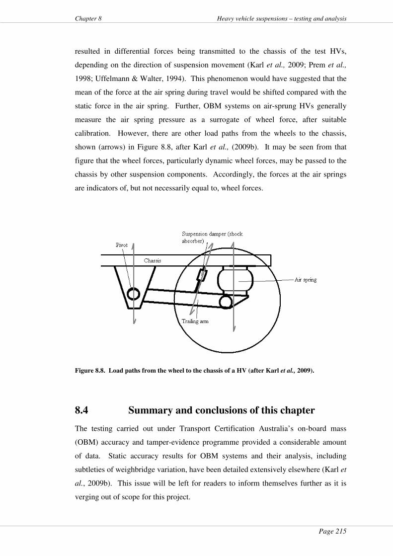
Page 215
Chapter 8 Heavy vehicle suspensions – testing and analysis
resulted in differential forces being transmitted to the chassis of the test HVs,
depending on the direction of suspension movement (Karl et al., 2009; Prem et al.,
1998; Uffelmann & Walter, 1994). This phenomenon would have suggested that the
mean of the force at the air spring during travel would be shifted compared with the
static force in the air spring. Further, OBM systems on air-sprung HVs generally
measure the air spring pressure as a surrogate of wheel force, after suitable
calibration. However, there are other load paths from the wheels to the chassis,
shown (arrows) in Figure 8.8, after Karl et al., (2009b). It may be seen from that
figure that the wheel forces, particularly dynamic wheel forces, may be passed to the
chassis by other suspension components. Accordingly, the forces at the air springs
are indicators of, but not necessarily equal to, wheel forces.
Figure 8.8. Load paths from the wheel to the chassis of a HV (after Karl et al., 2009).
8.4 Summary and conclusions of this chapter
The testing carried out under Transport Certification Australia’s on-board mass
(OBM) accuracy and tamper-evidence programme provided a considerable amount
of data. Static accuracy results for OBM systems and their analysis, including
subtleties of weighbridge variation, have been detailed extensively elsewhere (Karl et
al., 2009b). This issue will be left for readers to inform themselves further as it is
verging out of scope for this project.
Page 216
Heavy vehicle suspensions – testing and analysis Chapter 8
The accuracy results indicated strongly that, without particular preparation other than
calibration, 95 percent of contemporary OBM systems available in Australia are
accurate to +/- 500 kg; this being the offset values in the y-axis in Figure 8.2. The
results also indicated a total variation of 0.5 percent in OBM linearity for all (save
for three) OBM individual system tests (Figure 8.3). This was indicated from the
coefficient of determination (R2) values in the range 0.995 to 1.0, when the three
outliers were removed. Noting that the OBM systems were tested in “as presented”
condition, including being installed on hire HVs in some cases, this appeared to be a
very good result for jurisdictions and the OBM industry. Jurisdictions may now be
more confident about the performance of these systems, should they begin to specify
OBM as part of their regulatory frameworks. The details of such implementation
form part of Stage 2 of the Intelligent Access Program outlined in Section 1.5. With
some more refinement, the OBM industry may be able to better the figures found
from the testing. Implications for the OBM industry and jurisdictions will be
expanded in Chapter 12, Section 12.5.
8.5 Chapter close
8.5.1 General
This chapter presented results from the on-board mass (OBM) testing programme
conducted by Transport Certification Australia (TCA) where applicable to the project
“Heavy vehicle suspensions – testing and analysis”. These results were for the
straightforward portion of the test programme and informed the accuracy question
posed in Section 1.5.
Dynamic data from the air springs were introduced with some preliminary analysis
of the frequency spectra of non-tamper operating conditions. The tampering issue
was raised in Section 1.5 with some descriptions of the deliberate tampering events
during the tests detailed in Section 3.4.
The next chapter (Chapter 9) will expand on data analysis from the deliberate
tampering events, i.e. atypical conditions of operation for OBM systems. This will
lead to development of tamper indicators and include an algorithm to indicate a
tamper event. These indicators and the algorithm will be validated also in Chapter 9.
Page 217
Chapter 8 Heavy vehicle suspensions – testing and analysis
Links where this chapter informs other chapters of this thesis are shown in Figure
1.4.
“All government, indeed, every human benefit and enjoyment, every virtue and every prudent act, is founded on compromise and barter.” - Edmund Burke.
Page 218
Heavy vehicle suspensions – testing and analysis Chapter 9
9 Development of tamper metrics
9.1 About this chapter
This chapter details the development of metrics that would inform jurisdictions and
regulators of an attempt to tamper with an on-board mass (OBM) system on a heavy
vehicle (HV). Tampering events were deliberately introduced into the testing
(Section 3.4) for the OBM system accuracy and tamper-evidence work to meet
Objective 4. Oversight of the OBM testing was by Transport Certification Australia
as lead agency. Some data from that test programme contributed to the project
“Heavy vehicle suspensions – testing and analysis”.
9.2 Introduction
HV regulators regard tampering with vehicle instrumentation or measurement
systems, particularly those on heavy vehicles (HVs), as a major issue. Transport
Certification Australia was the lead agency for a test programme to determine
accuracy and tamper evidence for heavy vehicle on-board mass (OBM) systems
(Davis et al., 2008a, 2008b). Some controlled tampering was included in that test
programme to determine if the effects of that tampering could be detected from
changes in the data. This involved changing the operation of the test vehicles or their
systems. Those tampering events and the data derived contributed to the project
“Heavy vehicle suspensions – testing and analysis”.
Section 3.4.4 detailed the mechanism of interposing ball valves between the air
pressure transducers (APTs) and the air springs of the HVs tested. The dynamic data
from the air springs were recorded at various load points, depending on logistical
arrangements, for the open and closed states of the ball valves. The closed state
represented a deliberate tamper event. This was to simulate the instance where an
operator may block air lines to an OBM system in an attempt to under-report the
mass of the HV in order to overload it or, in the case of mass-distance charging
(Clarke & Prentice, 2009), reduce the charge for the trip, for instance.
Examples of data and analysis for the case where the ball valve was open (normal
operation) have been detailed in Chapter 8. The tamper events where the ball valve
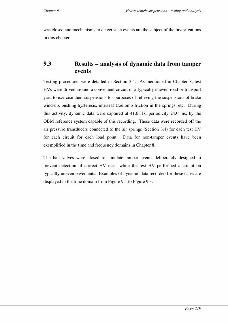
Page 219
Chapter 9 Heavy vehicle suspensions – testing and analysis
was closed and mechanisms to detect such events are the subject of the investigations
in this chapter.
9.3 Results – analysis of dynamic data from tamper
events
Testing procedures were detailed in Section 3.4. As mentioned in Chapter 8, test
HVs were driven around a convenient circuit of a typically uneven road or transport
yard to exercise their suspensions for purposes of relieving the suspensions of brake
wind-up, bushing hysteresis, interleaf Coulomb friction in the springs, etc. During
this activity, dynamic data were captured at 41.6 Hz, periodicity 24.0 ms, by the
OBM reference system capable of this recording. These data were recorded off the
air pressure transducers connected to the air springs (Section 3.4) for each test HV
for each circuit for each load point. Data for non-tamper events have been
exemplified in the time and frequency domains in Chapter 8.
The ball valves were closed to simulate tamper events deliberately designed to
prevent detection of correct HV mass while the test HV performed a circuit on
typically uneven pavements. Examples of dynamic data recorded for these cases are
displayed in the time domain from Figure 9.1 to Figure 9.3.

Page 220
Heavy vehicle suspensions – testing and analysis Chapter 9
Data from dynamic recording reference OBM system - LHS of HV
0
500
1000
1500
2000
2500
3000
3500
4000
0 2 4 6 8
10
12
14
16
18
20
22
24
26
28
Time (s)
Air
sp
rin
g r
ea
din
g (
kg
)
Drive axle LHS air spring
Trailer axle LHS air spring
Figure 9.1. Example of dynamic on-board mass data from an APT when tampering occurred.
The choice of left or right side, drive or trailer axle data in these figures was not
particularly significant; they are presented as illustrative of typical dynamic data
recorded during the tamper testing for all circuits and tested HVs. The plots of the
air spring data in Figure 9.1 indicate that the signal is steady, with some small
variation due to electronic noise present. It differs markedly from the dynamic data
that would be expected from air springs in the time domain as illustrated in (say)
Figure 8.4.
Figure 9.2 shows one case where one signal was similar to those in Figure 9.3 and
the other signal declined over time. This latter effect was due to a leak in the air line
between the APT and the ball valve, leading to a loss of pressure.
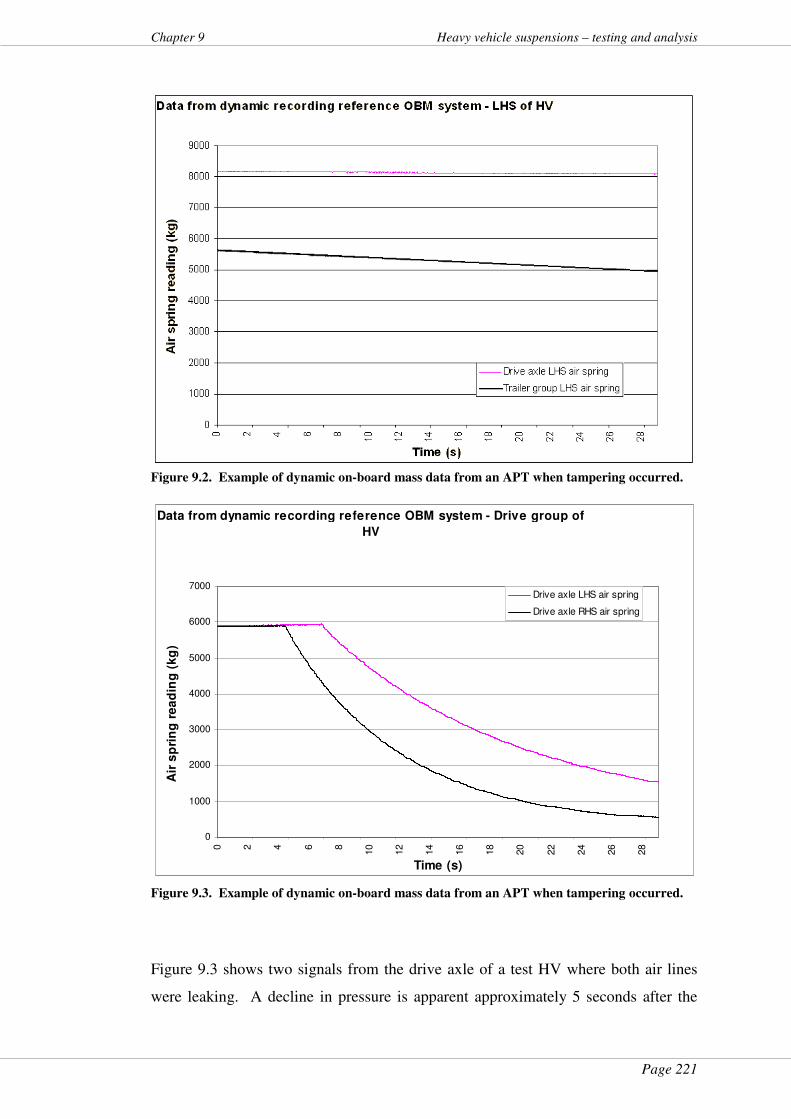
Page 221
Chapter 9 Heavy vehicle suspensions – testing and analysis
Figure 9.2. Example of dynamic on-board mass data from an APT when tampering occurred.
Data from dynamic recording reference OBM system - Drive group of
HV
0
1000
2000
3000
4000
5000
6000
7000
0 2 4 6 8
10
12
14
16
18
20
22
24
26
28
Time (s)
Air
sp
rin
g r
ea
din
g (
kg
)
Drive axle LHS air spring
Drive axle RHS air spring
Figure 9.3. Example of dynamic on-board mass data from an APT when tampering occurred.
Figure 9.3 shows two signals from the drive axle of a test HV where both air lines
were leaking. A decline in pressure is apparent approximately 5 seconds after the
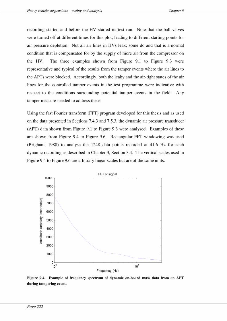
Page 222
Heavy vehicle suspensions – testing and analysis Chapter 9
recording started and before the HV started its test run. Note that the ball valves
were turned off at different times for this plot, leading to different starting points for
air pressure depletion. Not all air lines in HVs leak; some do and that is a normal
condition that is compensated for by the supply of more air from the compressor on
the HV. The three examples shown from Figure 9.1 to Figure 9.3 were
representative and typical of the results from the tamper events where the air lines to
the APTs were blocked. Accordingly, both the leaky and the air-tight states of the air
lines for the controlled tamper events in the test programme were indicative with
respect to the conditions surrounding potential tamper events in the field. Any
tamper measure needed to address these.
Using the fast Fourier transform (FFT) program developed for this thesis and as used
on the data presented in Sections 7.4.3 and 7.5.3, the dynamic air pressure transducer
(APT) data shown from Figure 9.1 to Figure 9.3 were analysed. Examples of these
are shown from Figure 9.4 to Figure 9.6. Rectangular FFT windowing was used
(Brigham, 1988) to analyse the 1248 data points recorded at 41.6 Hz for each
dynamic recording as described in Chapter 3, Section 3.4. The vertical scales used in
Figure 9.4 to Figure 9.6 are arbitrary linear scales but are of the same units.
100
101
0
1000
2000
3000
4000
5000
6000
7000
8000
9000
10000FFT of signal
Frequency (Hz)
am
plit
ude (
arb
itra
ry lin
ear
scale
)
Figure 9.4. Example of frequency spectrum of dynamic on-board mass data from an APT
during tampering event.
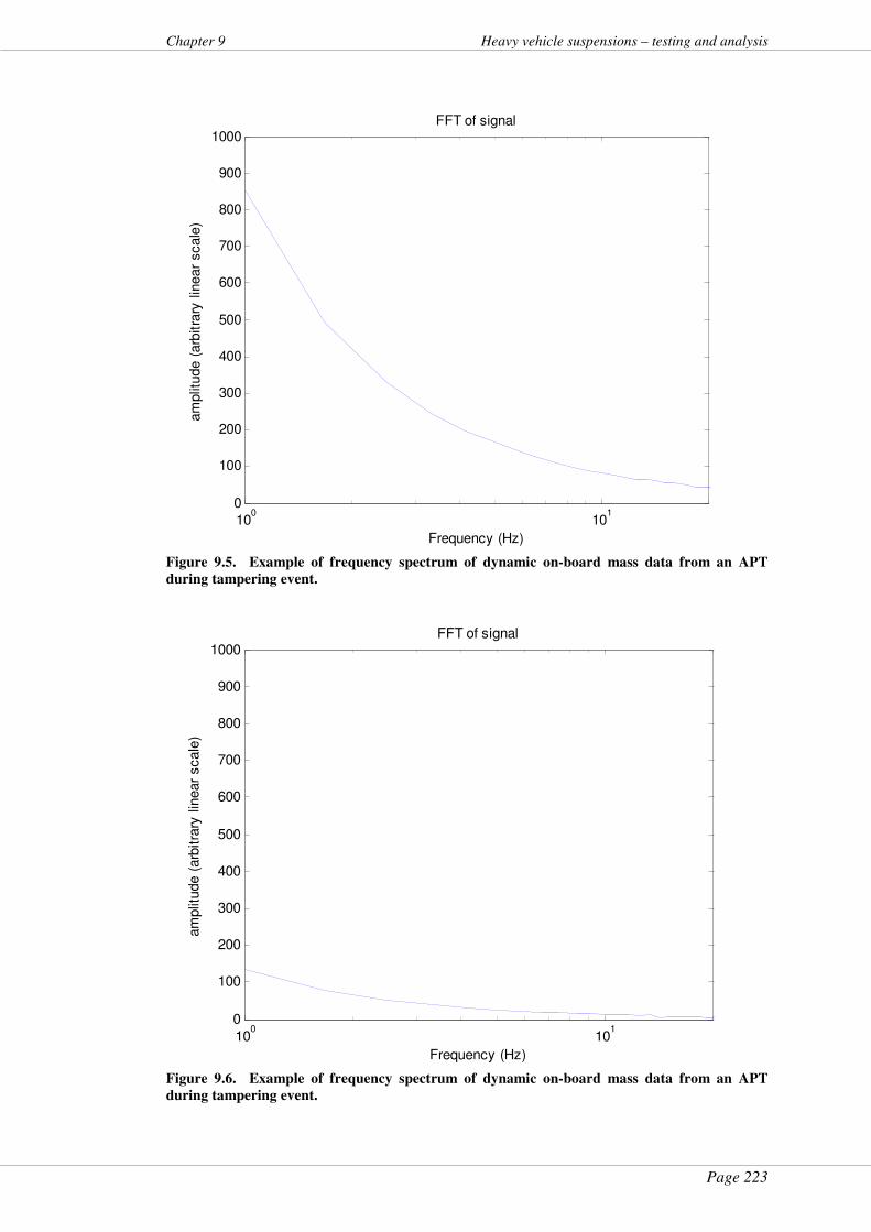
Page 223
Chapter 9 Heavy vehicle suspensions – testing and analysis
100
101
0
100
200
300
400
500
600
700
800
900
1000FFT of signal
Frequency (Hz)
am
plit
ude (
arb
itra
ry lin
ear
scale
)
Figure 9.5. Example of frequency spectrum of dynamic on-board mass data from an APT
during tampering event.
100
101
0
100
200
300
400
500
600
700
800
900
1000FFT of signal
Frequency (Hz)
am
plit
ude (
arb
itra
ry lin
ear
scale
)
Figure 9.6. Example of frequency spectrum of dynamic on-board mass data from an APT
during tampering event.
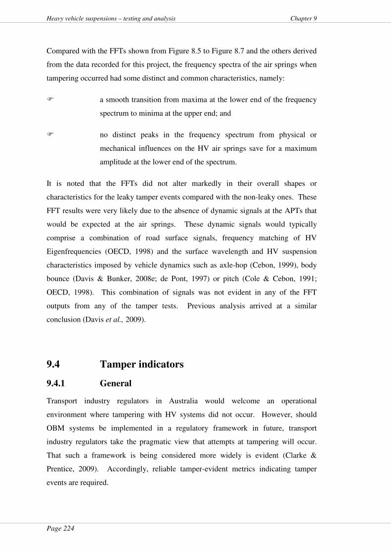
Page 224
Heavy vehicle suspensions – testing and analysis Chapter 9
Compared with the FFTs shown from Figure 8.5 to Figure 8.7 and the others derived
from the data recorded for this project, the frequency spectra of the air springs when
tampering occurred had some distinct and common characteristics, namely:
� a smooth transition from maxima at the lower end of the frequency
spectrum to minima at the upper end; and
� no distinct peaks in the frequency spectrum from physical or
mechanical influences on the HV air springs save for a maximum
amplitude at the lower end of the spectrum.
It is noted that the FFTs did not alter markedly in their overall shapes or
characteristics for the leaky tamper events compared with the non-leaky ones. These
FFT results were very likely due to the absence of dynamic signals at the APTs that
would be expected at the air springs. These dynamic signals would typically
comprise a combination of road surface signals, frequency matching of HV
Eigenfrequencies (OECD, 1998) and the surface wavelength and HV suspension
characteristics imposed by vehicle dynamics such as axle-hop (Cebon, 1999), body
bounce (Davis & Bunker, 2008e; de Pont, 1997) or pitch (Cole & Cebon, 1991;
OECD, 1998). This combination of signals was not evident in any of the FFT
outputs from any of the tamper tests. Previous analysis arrived at a similar
conclusion (Davis et al., 2009).
9.4 Tamper indicators
9.4.1 General
Transport industry regulators in Australia would welcome an operational
environment where tampering with HV systems did not occur. However, should
OBM systems be implemented in a regulatory framework in future, transport
industry regulators take the pragmatic view that attempts at tampering will occur.
That such a framework is being considered more widely is evident (Clarke &
Prentice, 2009). Accordingly, reliable tamper-evident metrics indicating tamper
events are required.
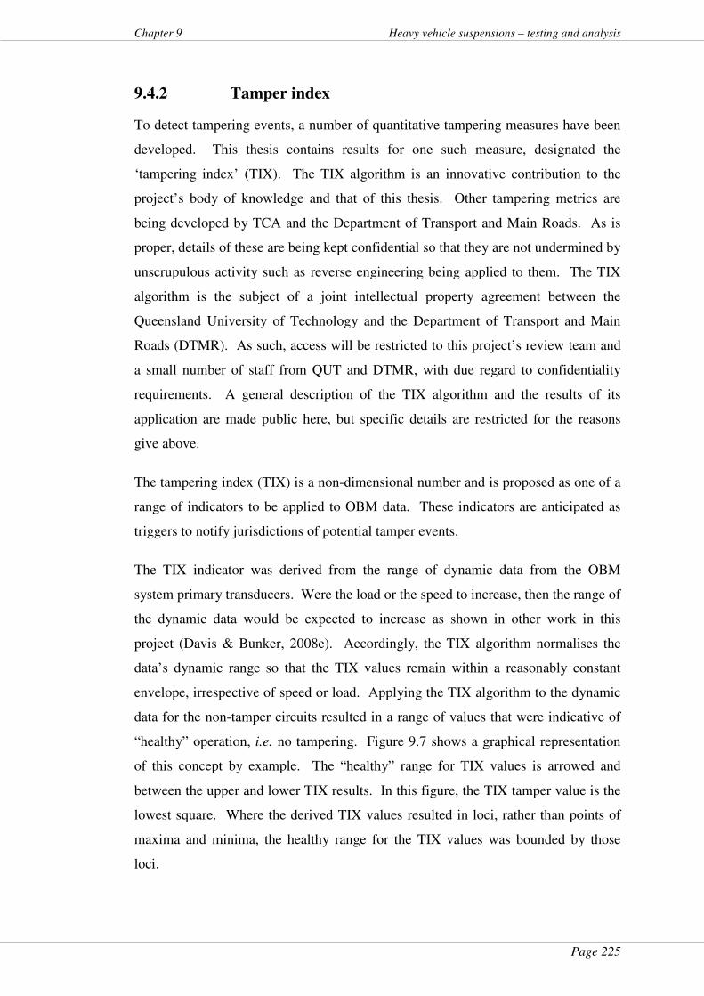
Page 225
Chapter 9 Heavy vehicle suspensions – testing and analysis
9.4.2 Tamper index
To detect tampering events, a number of quantitative tampering measures have been
developed. This thesis contains results for one such measure, designated the
‘tampering index’ (TIX). The TIX algorithm is an innovative contribution to the
project’s body of knowledge and that of this thesis. Other tampering metrics are
being developed by TCA and the Department of Transport and Main Roads. As is
proper, details of these are being kept confidential so that they are not undermined by
unscrupulous activity such as reverse engineering being applied to them. The TIX
algorithm is the subject of a joint intellectual property agreement between the
Queensland University of Technology and the Department of Transport and Main
Roads (DTMR). As such, access will be restricted to this project’s review team and
a small number of staff from QUT and DTMR, with due regard to confidentiality
requirements. A general description of the TIX algorithm and the results of its
application are made public here, but specific details are restricted for the reasons
give above.
The tampering index (TIX) is a non-dimensional number and is proposed as one of a
range of indicators to be applied to OBM data. These indicators are anticipated as
triggers to notify jurisdictions of potential tamper events.
The TIX indicator was derived from the range of dynamic data from the OBM
system primary transducers. Were the load or the speed to increase, then the range of
the dynamic data would be expected to increase as shown in other work in this
project (Davis & Bunker, 2008e). Accordingly, the TIX algorithm normalises the
data’s dynamic range so that the TIX values remain within a reasonably constant
envelope, irrespective of speed or load. Applying the TIX algorithm to the dynamic
data for the non-tamper circuits resulted in a range of values that were indicative of
“healthy” operation, i.e. no tampering. Figure 9.7 shows a graphical representation
of this concept by example. The “healthy” range for TIX values is arrowed and
between the upper and lower TIX results. In this figure, the TIX tamper value is the
lowest square. Where the derived TIX values resulted in loci, rather than points of
maxima and minima, the healthy range for the TIX values was bounded by those
loci.

Page 226
Heavy vehicle suspensions – testing and analysis Chapter 9
Figure 9.7. Illustrative plot showing TIX range for APT dynamic data during typical operation
and TIX value during tamper event.
The TIX algorithm was applied to the dynamic data recorded during the test circuits
(described in Section 8.3.2) for both the tamper and non-tamper test states. This was
to provide TIX values for control data when the HVs were moving without
tampering vs. test TIX values derived from controlled tamper events. Thirty-eight
instances of tamper vs. non-tamper events were analysed using the TIX algorithm.
Three indicative examples for this analysis are plotted Figure 9.8 to Figure 9.10
below.
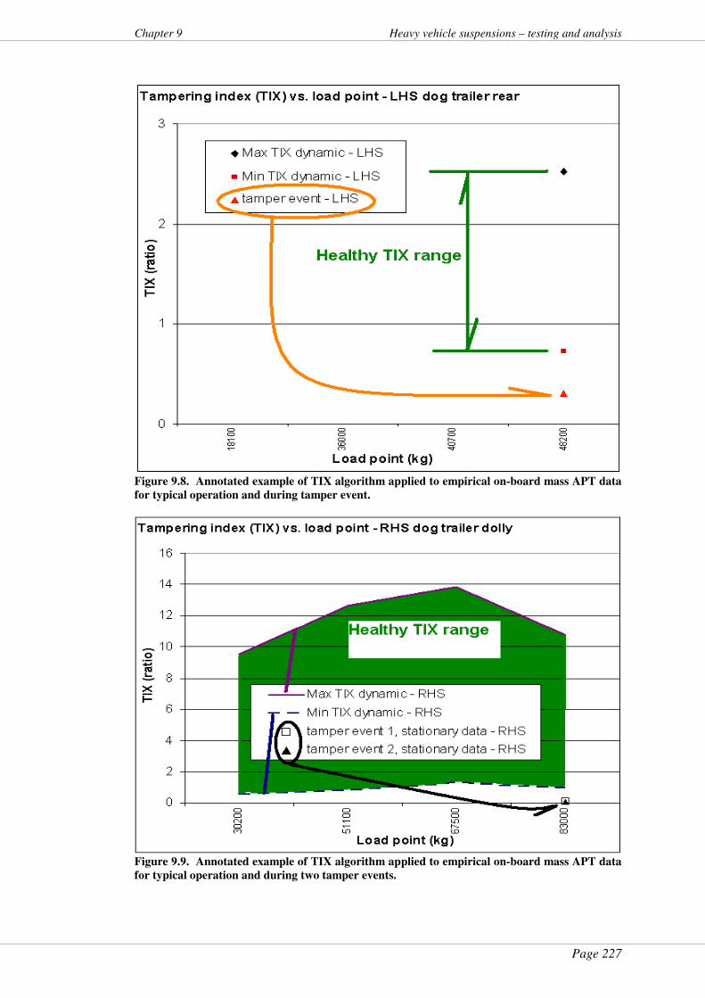
Page 227
Chapter 9 Heavy vehicle suspensions – testing and analysis
Figure 9.8. Annotated example of TIX algorithm applied to empirical on-board mass APT data
for typical operation and during tamper event.
Figure 9.9. Annotated example of TIX algorithm applied to empirical on-board mass APT data
for typical operation and during two tamper events.
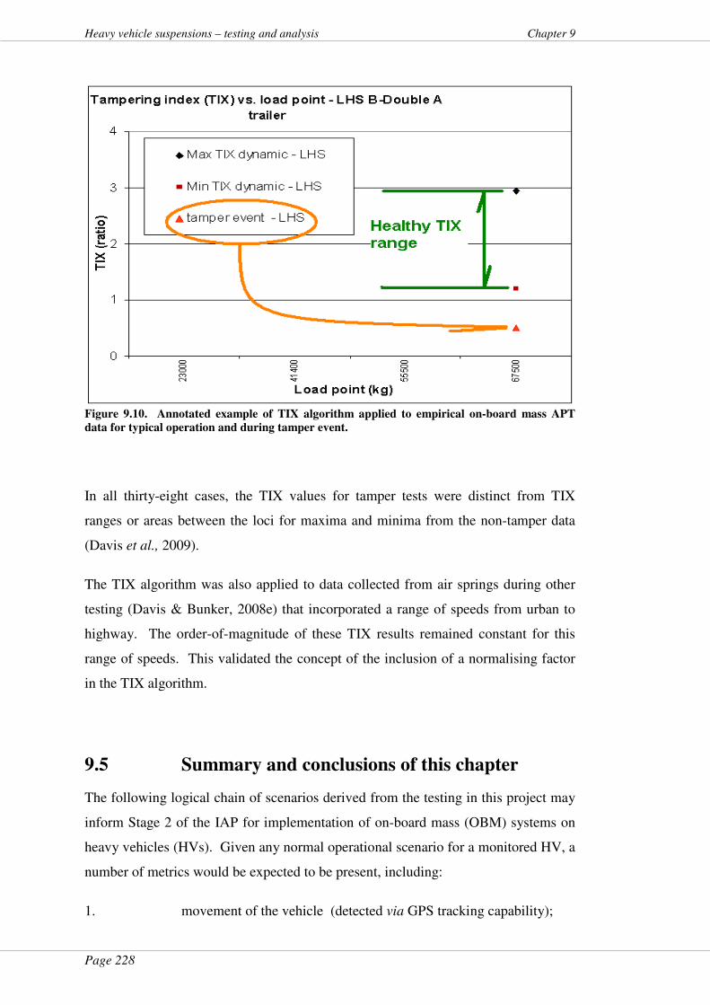
Page 228
Heavy vehicle suspensions – testing and analysis Chapter 9
Figure 9.10. Annotated example of TIX algorithm applied to empirical on-board mass APT
data for typical operation and during tamper event.
In all thirty-eight cases, the TIX values for tamper tests were distinct from TIX
ranges or areas between the loci for maxima and minima from the non-tamper data
(Davis et al., 2009).
The TIX algorithm was also applied to data collected from air springs during other
testing (Davis & Bunker, 2008e) that incorporated a range of speeds from urban to
highway. The order-of-magnitude of these TIX results remained constant for this
range of speeds. This validated the concept of the inclusion of a normalising factor
in the TIX algorithm.
9.5 Summary and conclusions of this chapter
The following logical chain of scenarios derived from the testing in this project may
inform Stage 2 of the IAP for implementation of on-board mass (OBM) systems on
heavy vehicles (HVs). Given any normal operational scenario for a monitored HV, a
number of metrics would be expected to be present, including:
1. movement of the vehicle (detected via GPS tracking capability);

Page 229
Chapter 9 Heavy vehicle suspensions – testing and analysis
2. frequency spectrum of the dynamic data being characterised as:
a. not smooth;
b. not declining in magnitude with increasing frequency;
c. with multiple peaks and all of them above (say) 1.0 Hz; and
3. tamper index (TIX) within healthy bounds.
Were scenarios 1 to 3 (and hence their associated metrics) to be present, then
tampering would be highly improbable.
Some OBM systems have an accelerometer built into their housing. These elements
are used by manufacturers to compensate the OBM reading when the HV is parked
on a slope. Other applications of accelerometers in OBM modules are used to
determine if the HV is on level ground. Both these applications of accelerometers to
OBM readings allow the HV operator to make a judgement of the reliability of the
OBM readout accuracy or, in more advanced applications, allow the OBM system to
correct the raw transducer data before displaying a mass value (Davis, 2008).
Further to scenarios 1 to 3 above, then, another indicator may be added:
4. dynamic signals from the chassis of the vehicle as it is in motion
and as measured by an accelerometer in the OBM unit.
Were a combination of scenario 1, above, to be present without scenarios 2 to 4, it is
highly likely that tampering has occurred.
Other combinations, such as where all or part of scenario 2 or scenario 3 were not
present individually but scenario 4 was detected, would indicate a high probability
that a tamper event had occurred.
Even for basic implementation of tamper-evidence without the multiple verifications
of scenarios 1 to 4 (and their associated metrics) above, the simple metrics of:
� movement of the vehicle, as detected by GPS;
� dynamic data being present at the chassis; and
Page 230
Heavy vehicle suspensions – testing and analysis Chapter 9
� absence of primary transducer signal (due to blocked air line or cables
cut);
would be a basic set of conditions that would indicate a high probability of a tamper
event.
Deliberate tampering with the OBM system of a HV is easier and more probable when
the vehicle is stationary compared with when it is moving. Accordingly, a tampering
event attempted when the HV were stationary should be able to be detected from analysis
of dynamic data by the use of the rules set out in this chapter. This issue and specification
of OBM systems, including sampling rates, will be discussed in detail in Chapter 12,
Section 12.5.
9.6 Chapter close
9.6.1 General
This chapter has presented typical tamper data from the heavy vehicle (HV) on-board
mass (OBM) testing programme conducted by Transport Certification Australia
(TCA) as applicable to the project “Heavy vehicle suspensions – testing and
analysis”. It has expanded on data analysis of the deliberate tampering events during
the OBM system testing.
A set of tamper indicators was developed and included an algorithm to indicate a
tamper event. This was to inform the tamper question posed in Section 1.5, with
some descriptions of the deliberate tampering events during the tests detailed in
Section 3.4. These indicators and the algorithm have been presented, with some
validation, in this chapter.
How these developments will inform road transport regulators and jurisdictions in
the implementation of OBM systems for HVs will be further expanded in Chapter 12
and concluded in Chapter 13. Links where this chapter informs other chapters of this
thesis are shown in Figure 1.4.
“Eternal vigilance is the price of liberty.” - Thomas Jefferson.
Page 231
Chapter 10 Heavy vehicle suspensions – testing and analysis
10 Dynamic load sharing and larger
longitudinal air lines for air-sprung heavy
vehicles
10.1 About this chapter
Chapter 2 covered a number of significant indicators for heavy vehicle (HV)
suspensions. This chapter (Chapter 10) has two purposes. The first is to meet
Objective 1 by documenting the development of a dynamic load sharing metric for
HV suspensions. The second, to meet Objective 2, is to apply this metric and some
of the suspension indicators, outlined in Chapter 2, to data from testing heavy vehicle
(HV) suspensions with larger longitudinal air lines to indicate whether larger
longitudinal air lines alter the suspension parameters of air-sprung HVs.
10.2 Introduction
10.2.1 Dynamic load sharing in heavy vehicles
Perfect load equalisation would result in a load sharing coefficient (LSC) of 1.0
(Potter et al., 1996). Early research into dynamic load sharing (Sweatman, 1983)
documented steel suspension LSCs in the range 0.791 to 0.957. That work placed air
suspensions somewhat in the top third of this range with LSCs of 0.904 to 0.925,
indicating that they did not necessarily load share any better than the steel
suspensions available at the time.
Previous work (Davis, 2006a; Davis & Sack, 2004) has shown that air-sprung “road
friendly” suspensions (RFS) do not load share dynamically when in multi-axle
groups. That testing, in February 2003 (Davis & Sack, 2004), was on a semi-trailer
fitted with “industry-standard” longitudinal air lines (6.5 mm inside diameter, 9.5
mm outside diameter). Note that there is not, strictly speaking, an “industry-
standard” air line size but the majority of air sprung HVs have air lines with inside
diameters ranging from approximately 4 mm to approximately 12 mm (Davis &
Sack, 2004; Simmons, 2005). Where “standard” is used to describe air line sizes in
this chapter, it is to this size range that this description refers. The results (Davis &
Sack, 2004) showed that the transfer of air between air springs on the test vehicle

Page 232
Heavy vehicle suspensions – testing and analysis Chapter 10
was in the order of three seconds. Were HV axle spacings 1 m apart at their closest
(worst case), then at 100 km/h (27.7 ms-1) the reaction time for air to transfer
between air springs would need to be in the order of 0.036 s for any reasonable
dynamic load sharing to occur. This value could be relaxed to about 0.047 s for axle
spacings of 1.3 m at 100 km/h. Hence, air transfer with time constants in the order of
three seconds will not load share dynamically. This inability causes potentially more
distress to the road network than the case where air-sprung HVs had an improved
ability to load-share (OECD, 1992, 1998).
Recent work has measured dynamic load sharing on tri-axle and quad-axle semi-
trailers (Blanksby, George, Peters et al., 2008; Blanksby et al., 2009). Even in light
of the unaddressed concerns within that body of research and further to Section 2.4.5,
that work showed load sharing in air-sprung HVs with industry-standard air lines
does not occur dynamically at urban speeds.
10.2.2 Dynamic load sharing in heavy vehicles – larger
longitudinal air lines
Two reports (Estill & Associates Pty Ltd, 2000; Roaduser Systems Pty Ltd, 2002)
were commissioned by the former National Road Transport Commission (NRTC)
after greater mass concessions were granted to HVs in Australia. These considered
countermeasures that corrected HV handling problems in air-suspended HVs.
Within those reports, HV air suspension modifications using larger-than-industry-
standard air lines were prominent. The nominated modifications were a commercial
system (the “Haire suspension system”) that used two 50 mm diameter air lines
longitudinally, along each side of an air-sprung HV, to connect fore-and-aft air
springs in lieu of the relatively smaller air lines normally used (Figure 3.5). These
air lines connect to the air springs via 20mm diameter connections (Figure 3.7). The
Roaduser report recommended tests to assess the effect of installing larger air lines
between sequential axles (Roaduser Systems Pty Ltd, 2002). That report ventured
the opinion that this measure should improve the load-sharing capability with two
reported cases where installation of such a system rectified handling problems.
Further, as far back as 2000, p. 32 of an Estill & Associates (2000) report
recommended that the NRTC, now the National Transport Commission (NTC):
Page 233
Chapter 10 Heavy vehicle suspensions – testing and analysis
“…investigate and evaluate ‘after market improvements’ to air suspensions…” from
installation of “…larger diameter pipes to supply and exhaust air flow to the bag
quickly and hence improve the response time of the air bag. The modification also
reduces the roll and has improved stability.”
Since those recommendations were made, the 2005 test programme funded by the
former Queensland Department of Main Roads (Davis, 2006a) and the 2007 test
programme (Davis, 2007; Davis & Kel, 2007) comprise the only known published
testing, to date, of HVs with larger longitudinal air lines.
10.2.3 Dynamic load sharing in heavy vehicles – regulatory
framework
As mentioned in Sections 1.3.1 and 1.3.2, air-sprung HVs were granted concessions
to carry greater mass at the end of the 1990s and this trend continues today,
conditional on their being fitted with “road friendly” (Australia Department of
Transport and Regional Services, 2004a, 2004b) suspensions.
Within the decision making process to allow HVs carrying greater mass in return for
being equipped with “road friendly suspensions”, Australian road authorities were
advised (OECD, 1992, 1998) that air-sprung HVs with industry-standard (or
conventionally sized) air lines between air springs did not load share in the dynamic
sense. The OECD research work found that ineffective dynamic load sharing had the
potential to cause greater road damage than might otherwise be the case were air-
sprung HVs to have improved dynamic load equalisation (OECD, 1992, 1998) over
and above that which was available at that time. Hence, the effects of poor dynamic
load equalisation were published and known at the time of granting air-sprung HVs
concessions to carry greater mass.
10.2.4 Objectives
One portion of the testing detailed in Section 3.2 was designed to produce data that
would allow comparison of suspension indicators for the control case of standard
longitudinal air lines vs. suspension indicators for the test case of larger longitudinal
air lines, the latter being the proprietary “Haire suspension system”. These results
Page 234
Heavy vehicle suspensions – testing and analysis Chapter 10
are shown in this chapter, allowing a commencement of meeting Objectives 1 and 2.
Alterations to dynamic load sharing for the case of the bus fitted with the “Haire
suspension system”, compared with its factory air lines, were not considered because
the bus drive axle had no other instrumented axle with which to “share” its load
(Section 3.2.1). However, results for alterations to the bus drive axle parameters,
other than dynamic load sharing (such as peak dynamic wheel forces and other
suspension metrics from Chapter 2), for the two cases of air line size have been
documented in this chapter alongside those derived for the other two HVs tested as
described in Section 3.2.
10.3 Larger longitudinal air lines
10.3.1 Dynamic load sharing – correlation metric
It should be possible to detect dynamic load sharing from cross-correlation of forces
between any two elements in a HV. Were dynamic load sharing occurring, any force
on one element, such as on an air spring or a wheel, should result in a force being
transferred to a corresponding element. Detecting the degree of correlation between
those pairs of forces should indicate the extent of dynamic load sharing; the higher
the correlation, the greater the amount of dynamic load sharing occurring. A similar
approach was attempted in Austroads project AT1212 (Blanksby et al., 2008;
Blanksby et al., 2009), but without definitive results. A contributory factor to the
indeterminate results from that test programme may have been that, with the
exception of removal of a shock absorber from the middle axle of the semi-trailer, no
control vs. test case data were recorded. Apparently, no other comparative testing
was undertaken during that programme (Blanksby et al., 2008; Blanksby et al.,
2009). Other issues, such as development of an algorithm to convert wheel force
correlation to a spatial measure, may have also contributed to the lack of definitive
conclusions from that test programme.
The testing detailed in Section 3.2 for the project Heavy vehicle suspensions – testing
and analysis followed the scientific method (Section 1.9.1) proposed generically by
Mill (1872). For the specific details of this project, standard air lines were the
control case and larger longitudinal air lines the test case. An innovative
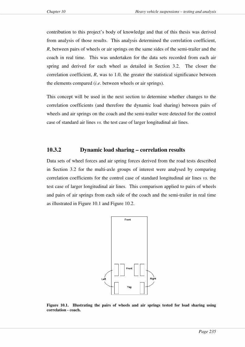
Page 235
Chapter 10 Heavy vehicle suspensions – testing and analysis
contribution to this project’s body of knowledge and that of this thesis was derived
from analysis of those results. This analysis determined the correlation coefficient,
R, between pairs of wheels or air springs on the same sides of the semi-trailer and the
coach in real time. This was undertaken for the data sets recorded from each air
spring and derived for each wheel as detailed in Section 3.2. The closer the
correlation coefficient, R, was to 1.0, the greater the statistical significance between
the elements compared (i.e. between wheels or air springs).
This concept will be used in the next section to determine whether changes to the
correlation coefficients (and therefore the dynamic load sharing) between pairs of
wheels and air springs on the coach and the semi-trailer were detected for the control
case of standard air lines vs. the test case of larger longitudinal air lines.
10.3.2 Dynamic load sharing – correlation results
Data sets of wheel forces and air spring forces derived from the road tests described
in Section 3.2 for the multi-axle groups of interest were analysed by comparing
correlation coefficients for the control case of standard longitudinal air lines vs. the
test case of larger longitudinal air lines. This comparison applied to pairs of wheels
and pairs of air springs from each side of the coach and the semi-trailer in real time
as illustrated in Figure 10.1 and Figure 10.2.
Figure 10.1. Illustrating the pairs of wheels and air springs tested for load sharing using
correlation - coach.
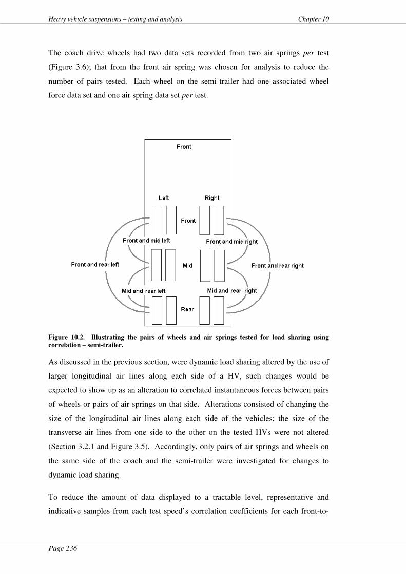
Page 236
Heavy vehicle suspensions – testing and analysis Chapter 10
The coach drive wheels had two data sets recorded from two air springs per test
(Figure 3.6); that from the front air spring was chosen for analysis to reduce the
number of pairs tested. Each wheel on the semi-trailer had one associated wheel
force data set and one air spring data set per test.
Figure 10.2. Illustrating the pairs of wheels and air springs tested for load sharing using
correlation – semi-trailer.
As discussed in the previous section, were dynamic load sharing altered by the use of
larger longitudinal air lines along each side of a HV, such changes would be
expected to show up as an alteration to correlated instantaneous forces between pairs
of wheels or pairs of air springs on that side. Alterations consisted of changing the
size of the longitudinal air lines along each side of the vehicles; the size of the
transverse air lines from one side to the other on the tested HVs were not altered
(Section 3.2.1 and Figure 3.5). Accordingly, only pairs of air springs and wheels on
the same side of the coach and the semi-trailer were investigated for changes to
dynamic load sharing.
To reduce the amount of data displayed to a tractable level, representative and
indicative samples from each test speed’s correlation coefficients for each front-to-
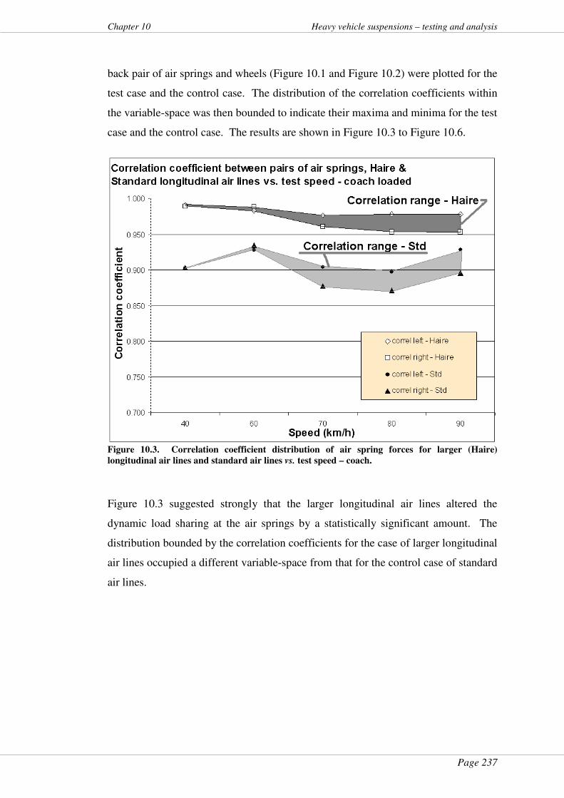
Page 237
Chapter 10 Heavy vehicle suspensions – testing and analysis
back pair of air springs and wheels (Figure 10.1 and Figure 10.2) were plotted for the
test case and the control case. The distribution of the correlation coefficients within
the variable-space was then bounded to indicate their maxima and minima for the test
case and the control case. The results are shown in Figure 10.3 to Figure 10.6.
Figure 10.3. Correlation coefficient distribution of air spring forces for larger (Haire)
longitudinal air lines and standard air lines vs. test speed – coach.
Figure 10.3 suggested strongly that the larger longitudinal air lines altered the
dynamic load sharing at the air springs by a statistically significant amount. The
distribution bounded by the correlation coefficients for the case of larger longitudinal
air lines occupied a different variable-space from that for the control case of standard
air lines.
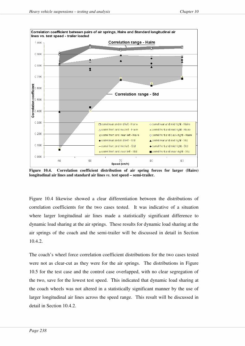
Page 238
Heavy vehicle suspensions – testing and analysis Chapter 10
Figure 10.4. Correlation coefficient distribution of air spring forces for larger (Haire)
longitudinal air lines and standard air lines vs. test speed – semi-trailer.
Figure 10.4 likewise showed a clear differentiation between the distributions of
correlation coefficients for the two cases tested. It was indicative of a situation
where larger longitudinal air lines made a statistically significant difference to
dynamic load sharing at the air springs. These results for dynamic load sharing at the
air springs of the coach and the semi-trailer will be discussed in detail in Section
10.4.2.
The coach’s wheel force correlation coefficient distributions for the two cases tested
were not as clear-cut as they were for the air springs. The distributions in Figure
10.5 for the test case and the control case overlapped, with no clear segregation of
the two, save for the lowest test speed. This indicated that dynamic load sharing at
the coach wheels was not altered in a statistically significant manner by the use of
larger longitudinal air lines across the speed range. This result will be discussed in
detail in Section 10.4.2.

Page 239
Chapter 10 Heavy vehicle suspensions – testing and analysis
Figure 10.5. Correlation coefficient distribution of wheel forces for larger (Haire) longitudinal
air lines and standard air lines vs. test speed – coach.
Similar to the results for the coach, those for the semi-trailer, illustrated in Figure
10.6, indicated that the distribution of wheel force correlation coefficients did not
alter by a statistically significant amount for the two cases of longitudinal air line
size.
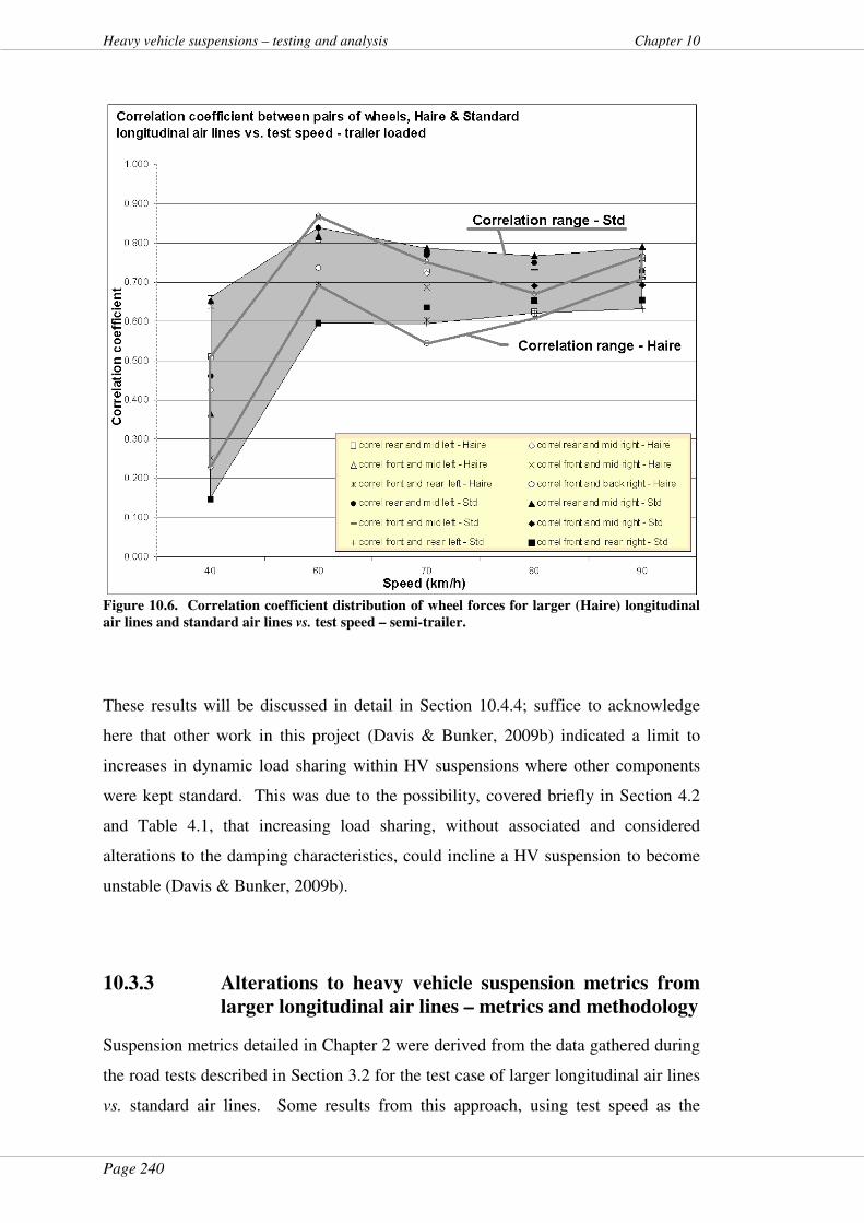
Page 240
Heavy vehicle suspensions – testing and analysis Chapter 10
Figure 10.6. Correlation coefficient distribution of wheel forces for larger (Haire) longitudinal
air lines and standard air lines vs. test speed – semi-trailer.
These results will be discussed in detail in Section 10.4.4; suffice to acknowledge
here that other work in this project (Davis & Bunker, 2009b) indicated a limit to
increases in dynamic load sharing within HV suspensions where other components
were kept standard. This was due to the possibility, covered briefly in Section 4.2
and Table 4.1, that increasing load sharing, without associated and considered
alterations to the damping characteristics, could incline a HV suspension to become
unstable (Davis & Bunker, 2009b).
10.3.3 Alterations to heavy vehicle suspension metrics from
larger longitudinal air lines – metrics and methodology
Suspension metrics detailed in Chapter 2 were derived from the data gathered during
the road tests described in Section 3.2 for the test case of larger longitudinal air lines
vs. standard air lines. Some results from this approach, using test speed as the

Page 241
Chapter 10 Heavy vehicle suspensions – testing and analysis
independent variable against which to plot the suspension metrics for the test case
and the control case, have been published elsewhere (Davis, 2006a, 2007; Davis &
Bunker, 2008d). An alternative approach to presenting derived suspension metrics
for the case of standard air lines as the control case and larger longitudinal air lines
as the test case is shown in the following section.
Section 7.3.1 detailed the development of a “novel roughness” measure or “novel
roughness” value. The values given by Sayers et al., (1986) were used as a guide to
develop a set of independent variables based on three bands of “novel roughness”
values. The bands, in “novel roughness” units of mm/m, were chosen as:
� below 3;
� from 3 to 4; and
� above 4.
These choices within the total range of the “novel roughness” values provided
approximately equal numbers of tests, and therefore roughly equal numbers of
suspension metrics, within each band. It is emphasised again here, as it was in
Section 7.3.1, that the “novel roughness” value was derived for each tested HV and
was not related to the IRI developed by Sayers et al., (1986).
The suspension metrics, detailed in Chapter 2, of dynamic load coefficient (DLC),
dynamic impact factor (DIF) and peak dynamic suspension force (PDSF) were
derived at the air springs of the bus for each of the “novel roughness” bands given
above. This was for both the cases of standard air lines as the control case and for
the test case of larger longitudinal air lines. Noting that the bus had no ability for its
drive axle to share load, neither the dynamic load sharing coefficient (DLSC), nor the
load sharing coefficient (LSC), were derived for that HV.
The same metrics were derived from wheel force data for the tests that used the two
sizes of longitudinal air lines. For suspension metrics using peak values, the peak
dynamic suspension force (PDSF) for air spring data mapped to peak dynamic wheel
force (PDWF) when using wheel data. The DLC, LSC, DIF and PDSF/PDWF at the
air springs and the wheels were derived for the coach and the trailer. Due to the
nature of the DLC and LSC metrics being specific to particular wheels or air springs,
Page 242
Heavy vehicle suspensions – testing and analysis Chapter 10
and to bring the data presented down to a tractable level, these values were averaged,
after derivation, across all wheels or all air springs within the group of interest. They
are shown in the tables below. Peak forces were not averaged; they were processed
as maxima with the results shown below.
The DLSC developed by de Pont (1997) was applied to the air spring data and the
wheel force data for the coach and the semi-trailer for the two cases of larger
longitudinal air lines. Individual results for each wheel or air spring compared with
the other wheels or air springs on that side of the HV were derived. This technique
altered the application of Equation 2.14 to deriving the DLSC for each air spring or
wheel using the forces measured at all of the air springs or wheels on the same side
as the particular air spring or wheel:
DLSCi = k
DLSDLS ii∑ − 2)(
Equation 10.1
where:
Dynamic load sharing (DLS) at wheel or air spring i =
∑=
=
=ni
i
i
ii
F
nFDLS
1
Equation 10.2
n = number of wheels or air springs on the side of wheel or air spring i;
Fi = instantaneous force at wheel or air spring i; and
k = number of instantaneous values of DLS, i.e. number of terms in the data set (de
Pont, 1997).
Similar to the work in Section 10.3.2, front-to-back dynamic load sharing alterations
arising from the use of larger longitudinal air lines was the focus since side-to-side
air line sizes had not been altered.
A t-test for variations in metrics for the two cases within each “novel roughness”
band was performed for the wheel force data and the air spring data. A
heteroscedastic test option was chosen since the data sets had unequal variances
Page 243
Chapter 10 Heavy vehicle suspensions – testing and analysis
(Kariya & Kurata, 2004) within each band of “novel roughness”. A conservative
value for α = 0.1 was chosen since, as mentioned in Chapter 7, road-damage
business cases generally use this α value as an upper bound. A one-tailed test
(StatPac Inc, 2007) was chosen since the results in Section 10.3.2 indicated that the
larger longitudinal air lines altered some dynamic measures in a particular direction.
A two-tailed test was considered but discarded since its other tail would have
informed the case for performance improvement beyond the confidence limit
(Hamburg, 1983).
Statistically significant variation between the control case and the test case was
tested. Where the results of the t-test indicated that there was a 90 percent or greater
probability (i.e. a result less than or equal to 0.1) that the population means of the
two cases varied due to the experimental difference and not error, these occurrences
are shown in shaded cells below. Where the t-test indicated this statistical
significance, the percentage change between the averaged derived parameter values
within each “novel roughness” band population for the two cases is shown
parenthetically.
10.3.4 Alterations to heavy vehicle suspension metrics at the
air springs from larger longitudinal air lines
A t-test for alterations in bus suspension metrics at the air springs was performed for
the different sized air lines. The results in Table 10.1 indicated that these alterations
did occur but not in a uniform manner across all “novel roughness” bands. Any
alterations to suspension metrics at this interface would likely not have been due to
any improvements to load sharing since there was no ability to shift air from the air
spring on one axle to another. Rather, where such alterations proved statistically
significant, the larger air lines were probably acting, as would an accumulator, to
reduce axle-to-chassis dynamic forces by compression of the relatively larger air
volume for the test case.
The phenomenon of extra compressible fluid acting as an accumulator to soften peak
dynamic forces has been hypothesised previously (Davis, 2007; Davis & Bunker,
2008d). Further, this possibility may have led to the result that alterations were not
consistent across all “novel roughness” bands due to standing waves in the lines.
Where improvements were evident, they were approximately 3 to 5 percent for the
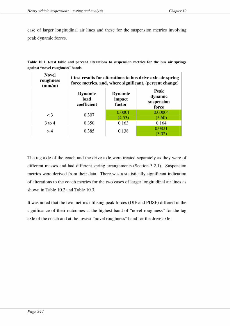
Page 244
Heavy vehicle suspensions – testing and analysis Chapter 10
case of larger longitudinal air lines and these for the suspension metrics involving
peak dynamic forces.
Table 10.1. t-test table and percent alterations to suspension metrics for the bus air springs
against “novel roughness” bands.
Novel
roughness
(mm/m)
t-test results for alterations to bus drive axle air spring
force metrics, and, where significant, (percent change)
Dynamic
load
coefficient
Dynamic
impact
factor
Peak
dynamic
suspension
force
< 3 0.307 0.0001 (4.53)
0.00004 (5.60)
3 to 4 0.350 0.163 0.164
> 4 0.385 0.138 0.0831 (3.02)
The tag axle of the coach and the drive axle were treated separately as they were of
different masses and had different spring arrangements (Section 3.2.1). Suspension
metrics were derived from their data. There was a statistically significant indication
of alterations to the coach metrics for the two cases of larger longitudinal air lines as
shown in Table 10.2 and Table 10.3.
It was noted that the two metrics utilising peak forces (DIF and PDSF) differed in the
significance of their outcomes at the highest band of “novel roughness” for the tag
axle of the coach and at the lowest “novel roughness” band for the drive axle.
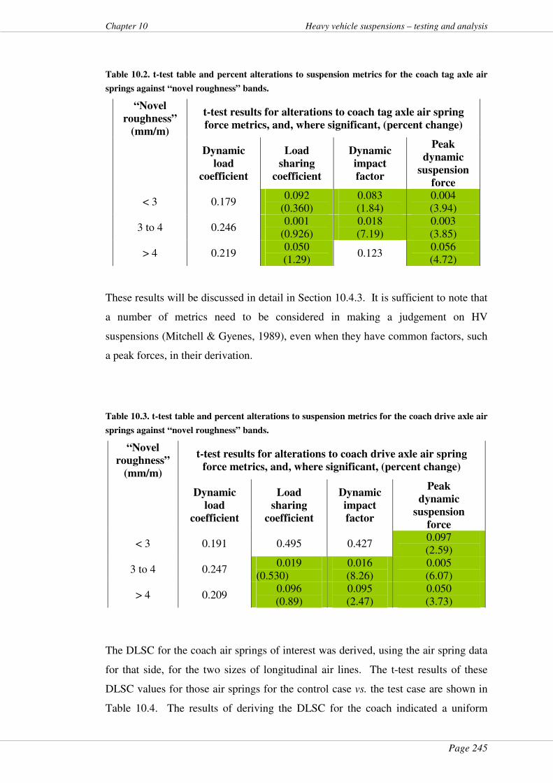
Page 245
Chapter 10 Heavy vehicle suspensions – testing and analysis
Table 10.2. t-test table and percent alterations to suspension metrics for the coach tag axle air
springs against “novel roughness” bands.
“Novel
roughness”
(mm/m)
t-test results for alterations to coach tag axle air spring
force metrics, and, where significant, (percent change)
Dynamic
load
coefficient
Load
sharing
coefficient
Dynamic
impact
factor
Peak
dynamic
suspension
force
< 3 0.179 0.092
(0.360) 0.083 (1.84)
0.004 (3.94)
3 to 4 0.246 0.001
(0.926) 0.018 (7.19)
0.003 (3.85)
> 4 0.219 0.050 (1.29)
0.123 0.056 (4.72)
These results will be discussed in detail in Section 10.4.3. It is sufficient to note that
a number of metrics need to be considered in making a judgement on HV
suspensions (Mitchell & Gyenes, 1989), even when they have common factors, such
a peak forces, in their derivation.
Table 10.3. t-test table and percent alterations to suspension metrics for the coach drive axle air
springs against “novel roughness” bands.
“Novel
roughness”
(mm/m)
t-test results for alterations to coach drive axle air spring
force metrics, and, where significant, (percent change)
Dynamic
load
coefficient
Load
sharing
coefficient
Dynamic
impact
factor
Peak
dynamic
suspension
force
< 3 0.191 0.495 0.427 0.097 (2.59)
3 to 4 0.247 0.019
(0.530)
0.016 (8.26)
0.005 (6.07)
> 4 0.209 0.096 (0.89)
0.095 (2.47)
0.050 (3.73)
The DLSC for the coach air springs of interest was derived, using the air spring data
for that side, for the two sizes of longitudinal air lines. The t-test results of these
DLSC values for those air springs for the control case vs. the test case are shown in
Table 10.4. The results of deriving the DLSC for the coach indicated a uniform
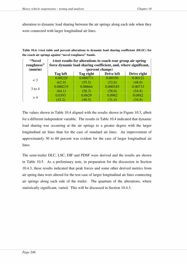
Page 246
Heavy vehicle suspensions – testing and analysis Chapter 10
alteration to dynamic load sharing between the air springs along each side when they
were connected with larger longitudinal air lines.
Table 10.4. t-test table and percent alterations to dynamic load sharing coefficient (DLSC) for
the coach air springs against “novel roughness” bands.
“Novel
roughness”
(mm/m)
t-test results for alterations to coach rear group air spring
force dynamic load sharing coefficient, and, where significant,
(percent change)
Tag left Tag right Drive left Drive right
< 3 0.00229 (62.9)
0.000771 (55.5)
0.00356 (52.6)
0.00121 (48.0)
3 to 4 0.000235
(64.1) 0.00664 (58.3)
0.000185 (58.0)
0.00733 (54.8)
> 4 0.0393 (43.2)
0.0629 (40.5)
0.0982 (31.4)
0.0882 (34.8)
The values shown in Table 10.4 aligned with the results shown in Figure 10.3, albeit
for a different independent variable. The results in Table 10.4 indicated that dynamic
load sharing was occurring at the air springs to a greater degree with the larger
longitudinal air lines than for the case of standard air lines. An improvement of
approximately 30 to 60 percent was evident for the case of larger longitudinal air
lines.
The semi-trailer DLC, LSC, DIF and PDSF were derived and the results are shown
in Table 10.5. As a preliminary note, in preparation for the discussion in Section
10.4.3, these results indicated that peak forces and some other derived metrics from
air spring data were altered for the test case of larger longitudinal air lines connecting
air springs along each side of the trailer. The quantum of the alterations, where
statistically significant, varied. This will be discussed in Section 10.4.3.
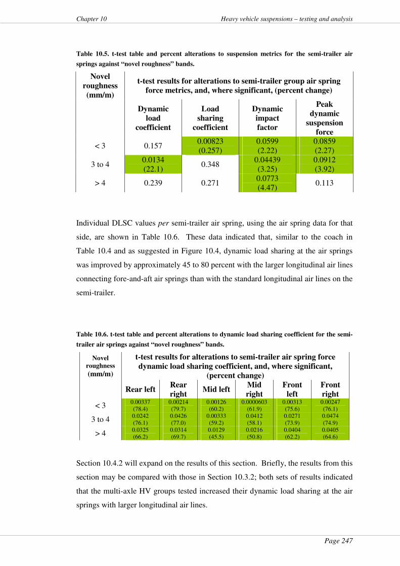
Page 247
Chapter 10 Heavy vehicle suspensions – testing and analysis
Table 10.5. t-test table and percent alterations to suspension metrics for the semi-trailer air
springs against “novel roughness” bands.
Novel
roughness
(mm/m)
t-test results for alterations to semi-trailer group air spring
force metrics, and, where significant, (percent change)
Dynamic
load
coefficient
Load
sharing
coefficient
Dynamic
impact
factor
Peak
dynamic
suspension
force
< 3 0.157 0.00823 (0.257)
0.0599 (2.22)
0.0859 (2.27)
3 to 4 0.0134 (22.1)
0.348 0.04439 (3.25)
0.0912 (3.92)
> 4 0.239 0.271 0.0773 (4.47)
0.113
Individual DLSC values per semi-trailer air spring, using the air spring data for that
side, are shown in Table 10.6. These data indicated that, similar to the coach in
Table 10.4 and as suggested in Figure 10.4, dynamic load sharing at the air springs
was improved by approximately 45 to 80 percent with the larger longitudinal air lines
connecting fore-and-aft air springs than with the standard longitudinal air lines on the
semi-trailer.
Table 10.6. t-test table and percent alterations to dynamic load sharing coefficient for the semi-
trailer air springs against “novel roughness” bands.
Novel
roughness (mm/m)
t-test results for alterations to semi-trailer air spring force
dynamic load sharing coefficient, and, where significant,
(percent change)
Rear left Rear
right Mid left
Mid
right
Front
left
Front
right
< 3 0.00337 (78.4)
0.00214 (79.7)
0.00126 (60.2)
0.0000603 (61.9)
0.00313 (75.6)
0.00247 (76.1)
3 to 4 0.0242 (76.1)
0.0426 (77.0)
0.00333 (59.2)
0.0412 (58.1)
0.0271 (73.9)
0.0474 (74.9)
> 4 0.0325 (66.2)
0.0314 (69.7)
0.0129 (45.5)
0.0216 (50.8)
0.0404 (62.2)
0.0405 (64.6)
Section 10.4.2 will expand on the results of this section. Briefly, the results from this
section may be compared with those in Section 10.3.2; both sets of results indicated
that the multi-axle HV groups tested increased their dynamic load sharing at the air
springs with larger longitudinal air lines.
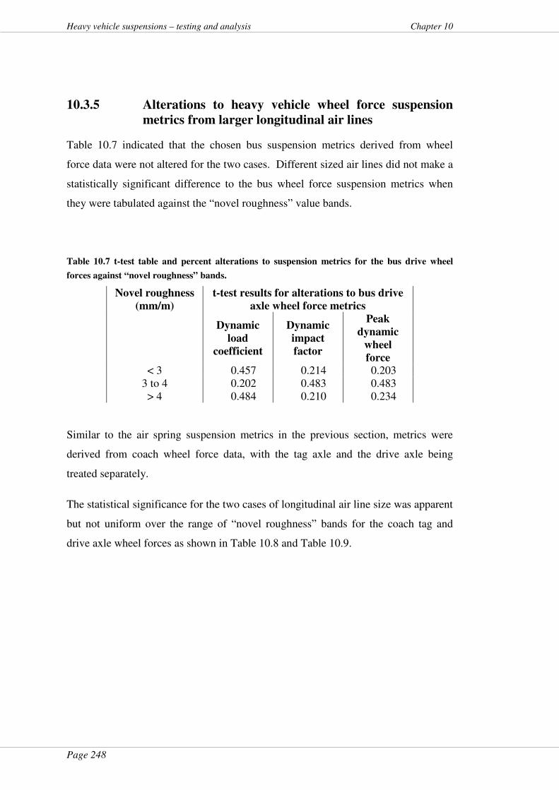
Page 248
Heavy vehicle suspensions – testing and analysis Chapter 10
10.3.5 Alterations to heavy vehicle wheel force suspension
metrics from larger longitudinal air lines
Table 10.7 indicated that the chosen bus suspension metrics derived from wheel
force data were not altered for the two cases. Different sized air lines did not make a
statistically significant difference to the bus wheel force suspension metrics when
they were tabulated against the “novel roughness” value bands.
Table 10.7 t-test table and percent alterations to suspension metrics for the bus drive wheel
forces against “novel roughness” bands.
Novel roughness
(mm/m)
t-test results for alterations to bus drive
axle wheel force metrics
Dynamic
load
coefficient
Dynamic
impact
factor
Peak
dynamic
wheel
force < 3 0.457 0.214 0.203
3 to 4 0.202 0.483 0.483 > 4 0.484 0.210 0.234
Similar to the air spring suspension metrics in the previous section, metrics were
derived from coach wheel force data, with the tag axle and the drive axle being
treated separately.
The statistical significance for the two cases of longitudinal air line size was apparent
but not uniform over the range of “novel roughness” bands for the coach tag and
drive axle wheel forces as shown in Table 10.8 and Table 10.9.
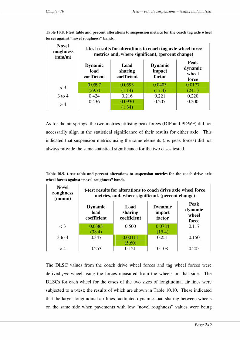
Page 249
Chapter 10 Heavy vehicle suspensions – testing and analysis
Table 10.8. t-test table and percent alterations to suspension metrics for the coach tag axle wheel
forces against “novel roughness” bands.
Novel
roughness
(mm/m)
t-test results for alterations to coach tag axle wheel force
metrics and, where significant, (percent change)
Dynamic
load
coefficient
Load
sharing
coefficient
Dynamic
impact
factor
Peak
dynamic
wheel
force
< 3 0.0597 (39.7)
0.0593 (1.14)
0.0403 (17.4)
0.0177 (24.1)
3 to 4 0.424 0.216 0.221 0.220
> 4 0.436 0.0930
(1.34) 0.205 0.200
As for the air springs, the two metrics utilising peak forces (DIF and PDWF) did not
necessarily align in the statistical significance of their results for either axle. This
indicated that suspension metrics using the same elements (i.e. peak forces) did not
always provide the same statistical significance for the two cases tested.
Table 10.9. t-test table and percent alterations to suspension metrics for the coach drive axle
wheel forces against “novel roughness” bands.
Novel
roughness
(mm/m)
t-test results for alterations to coach drive axle wheel force
metrics, and, where significant, (percent change)
Dynamic
load
coefficient
Load
sharing
coefficient
Dynamic
impact
factor
Peak
dynamic
wheel
force < 3 0.0383
(38.4) 0.500 0.0784
(15.4) 0.117
3 to 4 0.347 0.00111 (5.60)
0.251 0.150
> 4 0.253 0.121 0.108 0.205
The DLSC values from the coach drive wheel forces and tag wheel forces were
derived per wheel using the forces measured from the wheels on that side. The
DLSCs for each wheel for the cases of the two sizes of longitudinal air lines were
subjected to a t-test; the results of which are shown in Table 10.10. These indicated
that the larger longitudinal air lines facilitated dynamic load sharing between wheels
on the same side when pavements with low “novel roughness” values were being
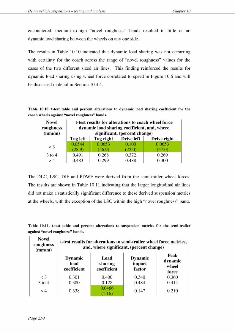
Page 250
Heavy vehicle suspensions – testing and analysis Chapter 10
encountered; medium–to-high “novel roughness” bands resulted in little or no
dynamic load sharing between the wheels on any one side.
The results in Table 10.10 indicated that dynamic load sharing was not occurring
with certainty for the coach across the range of “novel roughness” values for the
cases of the two different sized air lines. This finding reinforced the results for
dynamic load sharing using wheel force correlated to speed in Figure 10.6 and will
be discussed in detail in Section 10.4.4.
Table 10.10. t-test table and percent alterations to dynamic load sharing coefficient for the
coach wheels against “novel roughness” bands.
Novel
roughness
(mm/m)
t-test results for alterations to coach wheel force
dynamic load sharing coefficient, and, where
significant, (percent change)
Tag left Tag right Drive left Drive right
< 3 0.0544 (28.9)
0.0653 (56.9)
0.100 (22.0)
0.0653 (57.0)
3 to 4 0.491 0.268 0.372 0.269 > 4 0.483 0.299 0.488 0.300
The DLC, LSC, DIF and PDWF were derived from the semi-trailer wheel forces.
The results are shown in Table 10.11 indicating that the larger longitudinal air lines
did not make a statistically significant difference to these derived suspension metrics
at the wheels, with the exception of the LSC within the high “novel roughness” band.
Table 10.11. t-test table and percent alterations to suspension metrics for the semi-trailer
against “novel roughness” bands.
Novel
roughness
(mm/m)
t-test results for alterations to semi-trailer wheel force metrics,
and, where significant, (percent change)
Dynamic
load
coefficient
Load
sharing
coefficient
Dynamic
impact
factor
Peak
dynamic
wheel
force < 3 0.301 0.400 0.340 0.360
3 to 4 0.380 0.128 0.484 0.414
> 4 0.338 0.0466 (1.16)
0.147 0.210
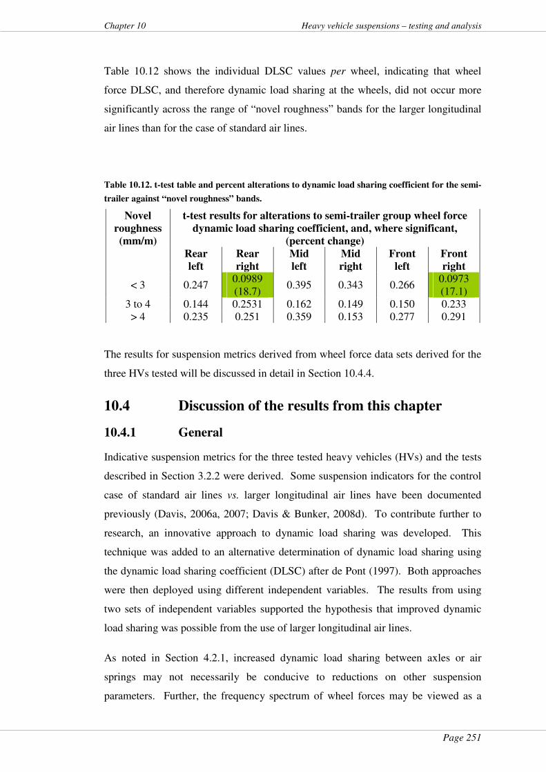
Page 251
Chapter 10 Heavy vehicle suspensions – testing and analysis
Table 10.12 shows the individual DLSC values per wheel, indicating that wheel
force DLSC, and therefore dynamic load sharing at the wheels, did not occur more
significantly across the range of “novel roughness” bands for the larger longitudinal
air lines than for the case of standard air lines.
Table 10.12. t-test table and percent alterations to dynamic load sharing coefficient for the semi-
trailer against “novel roughness” bands.
Novel
roughness
(mm/m)
t-test results for alterations to semi-trailer group wheel force
dynamic load sharing coefficient, and, where significant,
(percent change)
Rear
left
Rear
right
Mid
left
Mid
right
Front
left
Front
right
< 3 0.247 0.0989 (18.7)
0.395 0.343 0.266 0.0973 (17.1)
3 to 4 0.144 0.2531 0.162 0.149 0.150 0.233 > 4 0.235 0.251 0.359 0.153 0.277 0.291
The results for suspension metrics derived from wheel force data sets derived for the
three HVs tested will be discussed in detail in Section 10.4.4.
10.4 Discussion of the results from this chapter
10.4.1 General
Indicative suspension metrics for the three tested heavy vehicles (HVs) and the tests
described in Section 3.2.2 were derived. Some suspension indicators for the control
case of standard air lines vs. larger longitudinal air lines have been documented
previously (Davis, 2006a, 2007; Davis & Bunker, 2008d). To contribute further to
research, an innovative approach to dynamic load sharing was developed. This
technique was added to an alternative determination of dynamic load sharing using
the dynamic load sharing coefficient (DLSC) after de Pont (1997). Both approaches
were then deployed using different independent variables. The results from using
two sets of independent variables supported the hypothesis that improved dynamic
load sharing was possible from the use of larger longitudinal air lines.
As noted in Section 4.2.1, increased dynamic load sharing between axles or air
springs may not necessarily be conducive to reductions on other suspension
parameters. Further, the frequency spectrum of wheel forces may be viewed as a
Page 252
Heavy vehicle suspensions – testing and analysis Chapter 10
combination of body bounce and axle-hop (Section 7.4.3), the former predominantly
in the 1 to 4 Hz range, the latter in the 10 to 15 Hz range (Cebon, 1999; Davis &
Bunker, 2008e; de Pont, 1997). The results of the analysis of spring forces and
wheel forces will be treated separately in the following sections.
10.4.2 Alterations to air spring dynamic load sharing from
larger longitudinal air lines
Dynamic load sharing using correlated air spring force data was plotted against the
independent variable of test speed. This process indicated strongly that there was an
increase in dynamic load sharing for the test case of larger longitudinal air lines at
the axle-to-chassis interface for the multi-axle HVs tested (Figure 10.3 and Figure
10.4). These results were for an indicative range of correlations and indicative test
speeds and showed, in both of these figures, that the range of correlation coefficients
was separate and distinct for the two cases of air line size. The strong indicators
from the correlation coefficient approach required a different methodology to
determine if it was valid. The dynamic load sharing coefficient (DLSC) was applied
to the same air spring data but determined against a different independent variable in
the form of a range of “novel roughness” measure bands (Section 7.3.1) to separate
causality even further. This was to determine alterations to air spring DLSC along
either side of the coach and the semi-trailer for the two cases of air line size. The t-
test results for the DLSC alterations per air spring per side were uniform across all
“novel roughness” bands. It was noticeable that dynamic load sharing at the axle-to-
chassis interface, derived from the DLSC, improved across the board for the coach
and the trailer in the order of 30 to 80 percent. This result reinforced the validity of,
and results from, the correlation coefficient methodology.
Section 2.5 postulated that improvements to the dynamic load coefficient (DLC) and
the load sharing coefficient (LSC) were mutually exclusive. The results in Section
10.3.4 indicated that this might be the case for the air spring data from the two multi-
axle HVs tested; the LSC improved only when the DLC did not and vice versa. This
preliminary result will be left for other researchers to pursue since this is verging out
of scope.
Page 253
Chapter 10 Heavy vehicle suspensions – testing and analysis
10.4.3 Alterations to air spring suspension metrics from
larger longitudinal air lines
The dynamic load coefficient (DLC), the load sharing coefficient (LSC), dynamic
impact factor (DIF) and peak dynamic suspension force (PDSF) were derived from
air spring test data for different bands of the “novel roughness” metric. The results
were mixed but, overall, the larger longitudinal air lines made a statistically
significant difference to the derived metrics compared with the control case. The
metrics involving peak forces such as the PDSF and the DIF showed the most
consistent improvement. Whilst some metrics altered in a statistically significant
manner, the actual change, when averaged across the “novel roughness” band, was
sometimes below the margins of error (Appendix 2). After accounting for this,
improvements within the traditional suspension metrics such as the DLC, LSC, DIF
and PDSF, where they were statistically significant, varied in the order of 3 to 8
percent.
The bus had no other axle with which to “share” its dynamic load but some
alterations to the bus PDSF and the DIF were evident (Table 10.1) from the use of
larger longitudinal air lines. Accordingly, such alterations did not necessarily arise
from better dynamic load sharing (even though this phenomenon seemed to be
occurring between axles and wheels in the multi-axle HVs tested). Any alterations to
suspension metrics derived from the peak dynamic forces from any of the HVs tested
may have arisen from a combination of factors. One of these may have been
improved dynamic load sharing from the larger longitudinal air lines, as noted in the
previous section. The other factor, common to both the bus and the multi-axle HVs
tested, was an increased air volume contained in the larger air lines. This increased
air volume may have, it is suggested, compressed more readily over undulations and
acted as would gas in an accumulator, softening peak forces at the springs compared
with the control case (Davis, 2007; Davis & Bunker, 2008d).
10.4.4 Alterations to wheel force dynamic load sharing from
larger longitudinal air lines
In contrast to the results for the dynamic load sharing at the air springs, the results for
wheel force dynamic load sharing indicated a different outcome for the test case vs.
the control case of air line sizes. Figure 10.5 indicated that there was an
Page 254
Heavy vehicle suspensions – testing and analysis Chapter 10
improvement in dynamic load sharing for the case of larger longitudinal air lines at
the 40 km/h test speed. Otherwise, the two ranges of correlation coefficients for the
two cases overlapped without a distinct variation between them. The velocity of the
air in the air lines for low “novel roughness” and/or low speed would have been
relatively low compared with higher test speeds and/or higher “novel roughness” (Li
& McLean, 2003a, 2003b). Figure 10.5 indicated that, for the 40 km/h test speed
(i.e. low air line velocity) there was an improvement in the ability of the coach to
load share dynamically at the wheels in the case of the larger longitudinal air lines.
As a cross check, alterations in the coach DLSC for the case of low air flow (Table
10.10) indicated that dynamic load sharing was occurring during low “novel
roughness” events with an improvement of approximately 30 to 60 percent. This
was signified by the alteration in DLSC per wheel for all wheels, at the lowest
“novel roughness” band, compared with the other wheels on that side. This
agreement between the two approaches served as a useful verification of the validity
of the correlation coefficient as a determinant of dynamic load sharing against the
more mature DLSC metric.
Figure 10.6 indicated strongly that there was no difference in dynamic load sharing
at the semi-trailer wheels for the two cases of air line size since the correlation ranges
overlapped. This result suggested that dynamic load sharing did not alter at the
wheels of the semi-trailer for the increased air line size test case for any test speed.
Testing this contention for validity, as for the coach wheel forces, the wheel force
DLSC derived for the semi-trailer per wheel per side did not alter uniformly across
all wheels for any “novel roughness” band (Table 10.12).
10.4.5 Alterations to wheel force suspension metrics from
larger longitudinal air lines
Suspension metrics such as the dynamic load coefficient (DLC), the load sharing
coefficient (LSC), dynamic impact factor (DIF) and peak dynamic wheel force
(PDWF) were derived at the drive wheels of the bus for each of the “novel
roughness” bands given above. The results indicated that the bus wheel force
suspension metrics did not alter to a statistically significant degree for the two sizes
of air line tested.

Page 255
Chapter 10 Heavy vehicle suspensions – testing and analysis
The coach and the trailer had mixed results for suspension metrics derived from
wheel forces. Overall, the larger longitudinal air lines did not make a statistically
significant difference to the derived metrics compared with the control case, with the
exception of low flow events as noted above, although some metrics involving peak
dynamic forces were reduced by up to 24 percent in isolated cases. Section 4.2.1
developed a simple model of load sharing and indicated that an increase in dynamic
load sharing between wheels may increase the transmission of axle-hop from one
axle to the next. The frequencies of axle-hop have been shown in this project
(Section 7.4.3) and in other work (Cebon, 1999; Davis & Bunker, 2008e; de Pont,
1997) to range from 10 Hz to 15 Hz. These are the frequency ranges that coincide
with speeds of 60 km/h and above for axle spacings of 1.4 m. Both the coach and the
semi-trailer used for the testing described in Section 3.2 had axle spacings of 1.4 m.
Accordingly, the transmission of axle-hop frequencies, via improved dynamic load
sharing from one wheel or axle to the next, is not necessarily advantageous. The
possibility that continuous suspension oscillation at axle-hop frequencies would
occur with increased dynamic wheel load sharing has been explored in other work
during this project (Davis & Bunker, 2009b). This issue will be expanded in Chapter
12 by undertaking a sensitivity analysis for differing load sharing abilities of a HV
suspension model.
With regard to the DLC vs. LSC issue discussed in Section 2.5 and in the previous
section, with the exception of the tag axle at the low “novel roughness” band,
improvements in these two parameters derived from wheel forces for the two cases
of air line size were mutually exclusive. Further, the result for the LSC from the tag
axle at the lowest “novel roughness” band improved by less than the error value
(Appendix 2). Accordingly, the contention that DLC and LSC are mutually
exclusive may well still hold, given that detail. This issue will be left at that point as
a research avenue for the future since further pursuit of this concept is verging out-
of-scope.
Page 256
Heavy vehicle suspensions – testing and analysis Chapter 10
10.5 Summary and conclusions from this chapter
10.5.1 Alterations at the air springs from larger longitudinal
air lines
Two dynamic load sharing suspension metrics, the DLSC and the correlation
coefficient between pairs of air springs, were derived for the multi-axle heavy
vehicles (HVs) tested. These were shown to alter for the test case of larger
longitudinal air lines by a statistically significant degree leading to the conclusion
that dynamic load sharing was facilitated by larger air lines.
Other suspension metrics such as the PDSF and the DIF also altered for all three HVs
for the two cases tested. However, changes in these metrics, particularly for those
utilising peak force data, could not necessarily be separated in causality from the
alterations to the DLSC and the correlation coefficient between pairs of air springs.
This was due to increased volumes of compression media, in the form of more air in
the larger longitudinal air lines, between the air springs. Nonetheless, the results
indicated that, in the majority of cases, dynamic forces at the axle-to-chassis
interface were reduced by up to 8 percent with the use of the larger air lines. This
leads to the possibility that chassis and air spring forces could be reduced with the
implementation of this system. Further, approximate improvements from 30 and 80
percent in dynamic load sharing at the axle-to-chassis interface occurred with the
larger longitudinal air lines.
A preliminary observation may be that improving dynamic load sharing does not
necessarily lead to improvements in other suspension metrics. These results and
issues associated with altering the dynamics between air springs will be explored in
Chapter 12.
10.5.2 Alterations at the wheels from larger longitudinal air
lines
For the HVs with multi-axle suspension arrangements, the suspension metrics
associated directly with dynamic load sharing at the wheels did not alter in a
statistically significant manner across the “novel roughness” bands for the case of
larger longitudinal air lines. Some alterations to dynamic load sharing at the coach
Page 257
Chapter 10 Heavy vehicle suspensions – testing and analysis
wheels did occur in a statistically significant manner during low air line flow events.
Suspension metrics involving peak dynamic forces altered by up to approximately 24
percent for the test case. However, this range of improvement was not consistent
across all wheels and it was not consistent across all roughness bands or speeds.
Alterations to other suspension metrics for all HVs tested, such as the PDWF and the
DIF, did not alter in the majority of cases for the test air line size case vs. the control
case. Increased dynamic load sharing at the wheels was explored briefly in terms of
any potential instability arising from continued oscillations, at axle-hop frequencies,
leading to undesirable consequences with respect to vehicle stability. Given the
presence of moderate numbers of “Haire suspension systems” in the Australian HV
fleet without obvious distress or HV instability (Estill & Associates Pty Ltd, 2000;
Roaduser Systems Pty Ltd, 2002), the operational evidence suggests that forces due
to axle-hop frequencies are not shared dynamically at the wheels for either size of
longitudinal air line. This contention matches with the analysis of the results from
this chapter.
10.6 Chapter close
This chapter presented analysis of data gathered as described in Section 3.2.2 using
some of the suspension metrics from Chapter 2. An innovative method of
determining the presence of dynamic load sharing was also developed using the
correlation of forces between pairs of heavy vehicle (HV) components such as
wheels or air springs.
Indicative air spring and wheel force data from this analysis were plotted against test
speed as the independent variable. Some of the suspension metrics from Chapter 2
were derived for air spring and wheel force data and presented using a range of
“novel roughness” bands (Section 7.3.1) as the independent variable. Both these
approaches indicated that the issue of larger longitudinal air lines increasing dynamic
load sharing at the air springs of the tested HVs has, in general, been resolved in the
affirmative.
Any dynamic load sharing improvement at the wheels due to larger longitudinal air
Page 258
Heavy vehicle suspensions – testing and analysis Chapter 10
lines was not evident save for low speed/low “novel roughness” events. This was not
unexpected since increases in wheel force dynamic load sharing would incline
potentially undesirable axle-hop oscillations to propagate continuously during travel.
This issue will be explored in Chapter 12 by undertaking a sensitivity analysis for
differing load sharing abilities of a HV suspension model.
Links where this chapter informs other chapters of this thesis are shown in Figure
1.4.
“What I dream of is an art of balance.”- Henri Matisse.
Page 259
Chapter 11 Heavy vehicle suspensions – testing and analysis
11 Heavy vehicle in-service suspension testing
11.1 About this chapter
Chapter 1, Section 1.4 detailed the rationale behind in-service heavy vehicle (HV)
suspension testing. To meet Objective 3, two low-cost HV suspension tests were
developed. Chapter 6 detailed the results for a “proof-of-concept” low-cost HV
suspension test that excited a HV suspension during the traverse of a 50 mm steel
pipe and measured the air spring response. Chapter 7, Section 7.5 detailed the results
of a second, low cost HV suspension test using a modified brake testing machine.
This chapter explores the outcomes of those tests in terms of a discussion about the
policy and strategic implication of an in-service HV suspension test regime. This
will lead on to a discussion on the contribution to knowledge from this project in
Chapter 12.
11.2 Introduction
11.2.1 General
Heavy vehicles (HVs) with “road friendly” suspensions (RFS) were granted
concessions to carry greater masses under the various higher mass limits (HML)
schemes (Section 1.4.1) arising from some of the micro-economic reforms in
Australia over the last 15 years. The HV suspension requirements under HML
schemes in Australia broadly followed the European assumption that air suspensions
on HVs should be allowed a payload advantage over conventional steel-sprung axles
based on “damage equivalence” (de Pont, 1997). The health of HV suspensions and
the related effect on the road network asset when they move out-of-specification has
been well documented (Gyenes & Mitchell, 1992; National Road Transport
Commission, 1993; OECD, 1998). That air suspensions, deemed to be “road
friendly” at the time and fitted to HVs carrying HML loads, remained healthy was
recommended as one of the conditions of access (Pearson & Mass Limits Review
Steering Committee, 1996a).
Australia incorporated the 92/7/EEC parameters and tests into its VSB 11
certification regime for “road friendly” suspensions as well as adding additional
Page 260
Heavy vehicle suspensions – testing and analysis Chapter 11
requirements regarding static load sharing. “Road friendly” suspensions in Australia
generally incorporate air springs, although some steel RFS have come onto the
market (Australia Department of Transport and Regional Services, 2004b).
11.2.2 In-service suspension testing of HVs in Australia
Methods to determine the health of air-sprung HV suspensions were proposed before
their introduction into Australia (Cebon, 1999; Potter et al., 1997; Woodrooffe, 1995;
Woodrooffe et al., 1988). A specification was developed, Vehicle Standards Bulletin
11 (Australia Department of Transport and Regional Services, 2004a, 2004c). This
Vehicle Standards Bulletin (VSB) was applied to new suspensions going into service
on HVs carrying out HML duties. An in-service suspension test was not specified at
the time.
The bi-lateral infrastructure funding agreements (BIFAs) in force between both the
State Governments of New South Wales and Queensland with the Australian
Government at the time of writing contain commitments to develop an in-service test
for air-sprung HVs operating under HML schemes. A project by the National
Transport Commission (NTC) to develop such a test is now underway.
The NTC’s brief for the consultancy to that project stated, in part:
..."The objective of this consultancy is to identify and report (with recommendations)
on devices that will deliver:
� an in-service field test for road friendly suspension systems
including consideration of dynamometer testing or other low
cost test methods; and
� a roadside enforcement test..."
Note the emphasis on "low-cost test methods".
As inputs to that NTC project, the former Queensland Department of Main Roads
(now part of the Department of Transport and Main Roads) has (amongst other
efforts) contributed in-kind support, via a joint project with QUT entitled Heavy
vehicle suspensions – testing and analysis (Davis, 2007, 2008; Davis & Bunker,
Page 261
Chapter 11 Heavy vehicle suspensions – testing and analysis
2007, 2008a, 2008b, 2008c, 2008d, 2008e, 2009; Davis & Kel, 2007; Davis, Kel, &
Sack, 2007). The joint project used data from (former Main Roads’) low-cost and
preliminary test programmes carried out on a limited scale (Davis & Sack, 2004,
2006) as well as major and subsequent testing work (Davis, 2007, 2008; Davis &
Bunker, 2008c, 2008d, 2008e, 2009; Davis & Kel, 2007; Davis et al., 2007).
11.2.3 In-service HV testing in the transport environment
Any test on the air suspensions of the HV fleet operating at HML in Australia would
need to be low-cost, given the tight financial margins on which road transport
operates. VSB 11 type-testing is comparatively expensive with an order of
magnitude of $AUD5,000 per test (Bisitecniks, 2007). This cost is for either single
axles or axles in a group. A cost structure of this magnitude would not be acceptable
for testing every air-sprung axle on every HV operating under the various HML
schemes in Australia. This point especially since the tests would conceivably need to
be done annually for typical operation and more frequently under arduous conditions.
To achieve acceptance of in-service testing of air-sprung HV suspensions the costs
per test would have to be one or two orders-of-magnitude lower than for VSB 11
testing.
11.3 In-service HV suspension testing – issues and
discussion
11.3.1 Test standards for in-service HV testing
The standard defining RFS characteristics in Australia at the time of writing is VSB
11. Various regulations govern HVs operating at HML loads. One of these is the
requirement for HVs operating at HML loads to be equipped with RFS as they go
into service. Their suspensions are certified to VSB 11, by definition. VSB 11 is
structured such that a “type test” of one axle at varying loadings is then applicable to
that suspension model across the range of installations on HVs, including multi-axle
installations. The issue of load sharing between axles tested singly is not addressed
definitively in VSB 11 (Davis & Bunker, 2007). Further, the composition of VSB 11
Page 262
Heavy vehicle suspensions – testing and analysis Chapter 11
is well suited to the laboratory situation but not as an application appropriate to
testing a large volume of HVs.
Despite the issue noted above regarding a low-cost test, any proposal for an in-
service test on HV suspensions faces a challenge as defined by the following logic:
� RFS are certified to VSB 11 at the time the HV so equipped
commences HML service (usually when new);
� the HV operator is required to maintain the HV suspension such
that it keeps its characteristics within the bounds of VSB 11;
� since there is no other definition of “road friendliness”,
jurisdictions wishing to specify a test for in-service HV
suspension characteristics have, at the time of writing, no other
choice but to specify VSB 11;
� therefore, jurisdictions testing a HV for RFS compliance in an in-
service environment have no choice, at the time of writing, but to
use VSB 11 and suffer the higher costs accordingly.
This chain of logic leads to the conclusion that the only RFS test that is acceptable in
Australia at present is VSB 11, in-service or otherwise. Given the nature of VSB 11
as a “type test” more suited to laboratory environments, and as noted above, VSB 11
testing is relatively expensive.
Low cost testing, such as the “proof-of-concept” testing documented in Chapter 6 for
the “pipe test” excitation and in Chapter 7, Section 7.5 for the roller bed, are not
recognised test methods. Further, there are no low-cost methods for determining
VSB 11 compliance. This would seem to be a challenge for regulators at the time of
writing. Similar situations have, however, been resolved in the past by jurisdictions.
This was usually by specifying a different standard for the new state vs. any in-
service requirements. A simple example would be tyre groove depth: the tyre is
installed by the retailer and is covered by the applicable standards for new tyres. The
vehicle owner replaces the tyre when the groove depth reaches a minimum value as
specified by the appropriate regulator. The tyre, by definition, never meets its “as
new” specifications during its lifetime but provides service until worn out. It is
Page 263
Chapter 11 Heavy vehicle suspensions – testing and analysis
suggested that a similar pragmatic relaxation of the “as new” requirements for RFS
specifications should occur for in-service suspension testing of HVs.
These issues will need to be addressed by the NTC in developing in-service test
standards for RFS suspensions.
11.3.2 In-service HV testing & on-board mass measurement
systems
On-board mass (OBM) systems are becoming increasingly prevalent in Australia’s
HV fleet. The national project to determine the feasibility of OBM systems in a
regulatory framework has formed part of the project for this thesis (Davis et al.,
2008a, 2008b; Karl, 2007; Karl et al., 2009). Chapter 8 showed that 95 percent of
OBM systems available commercially were accurate to within +/- 500 kg. Further,
the results from the reference system and one other used for the testing described in
Chapter 8 (Karl et al., 2009b) indicated that reliable dynamic data were available
from OBM systems. As noted in Section 3.4.2, most OBM manufacturers have
supplied sufficient information to the OBM project team to indicate that dynamic
data from air springs or accelerometers could be recorded by OBM systems (Davis,
2008).
A HV may be subjected to an impulse of appropriate magnitude and duration, such
as would result from traversing a slightly protruding bar embedded conveniently in a
transport operator’s marshalling yard. An OBM system of appropriate sampling
speed may record the data from the air springs or chassis accelerometers of that HV.
The resultant signals from such data could be analysed for body bounce and damping
ratio, i.e. VSB 11 characteristics. This technique need not be confined to air-
suspended HVs; analysis of steel-suspended HV chassis acceleration would be
applicable.

Page 264
Heavy vehicle suspensions – testing and analysis Chapter 11
11.3.3 In-service HV testing – impulse testing and a way
forward
The dilemma outlined in Section 11.3.1 becomes slightly more difficult when the
results of differences in test methods are examined. Uffelmann and Walter (1994)
noted differences in damping ratio results of over 60 percent, depending on
suspension test method and excitation impulse direction. Further, Sweatman et al.,
(2000) allowed a margin of 25 percent between an in-service value for damping ratio
and the acceptable threshold for damping ratio under VSB 11. The parameters
derived from exciting HV suspensions using the “pipe test” (Chapter 6) indicated an
envelope of inaccuracy of approximately 16 percent from the manufacturer’s VSB
data or data generated from VSB 11-style step tests. Given the difference in
excitation functions between the “pipe test” and the VSB 11 results, this error was
relatively small compared with that found by the previous research of Uffelmann and
Walter (1994).
Some of these issues would be mitigated were HV operators to perform their own
testing under (say) the National Heavy Vehicle Accreditation Scheme (NHVAS).
The NHVAS is a national scheme for HVs to meet “alternative compliance
procedures” to those enforced by road authorities. It specifies that HV operators
abide by a set of standards, management procedures, audits and business rules.
There are two modules under NHVAS, maintenance management and mass
management. HV operators may choose accreditation in one or both modules.
Accreditation is recognised across Australia. Jurisdictional representatives perform
regular audits on HV operators accredited under NHVAS to ensure that the
provisions are met (National Transport Commission, 2008).
An in-service test would not need to be particularly accurate if the suspension in
question were monitored over some months, under arduous service; or years, in
suburban service, under a scheme such as NHVAS. The indicative inaccuracy of
approximately 16 percent between the “pipe test” results and VSB 11 test results may
be acceptable for pass/fail field testing. By testing a HV when new, the errors
between VSB 11 values and any in-service test would be clear and, even with
inaccuracies due to test method, constant. Accordingly, the in-service test results for
that HV suspension would become calibrated against the certified VSB 11
Page 265
Chapter 11 Heavy vehicle suspensions – testing and analysis
parameters of the HV axle when new. Further, the margins of error between the new
values for the suspensions tested and those for (say) the “pipe test” results for this
project could be accommodated by plotting the histories of test results. After the
suspension reached some threshold, it could be referred to a more precise
measurement technique or simply have its shock absorbers (and bushes, etc.)
replaced as a matter of course when the HV next came in for servicing.
A pipe or other suitable discontinuity such as used for the testing in this project could
be installed in the driveway of a transport facility. Other discontinuities such as
increasingly prevalent speed bumps in transport yards may also suffice as forcing
functions. With the increasing prevalence of on-board-mass (OBM) measurement
systems installed on HVs, such a traverse would result in an OBM system record of
air spring or chassis accelerometer data. Were the HV loaded appropriately, these
data could be analysed to determine body bounce damping ratio and damped natural
frequency (Davis et al., 2007; Davis & Sack, 2004, 2006) within known margins of
error as shown in Chapter 6. Any suitable discontinuity such as a bar, pipe or
channel would suffice were it of sufficient height to elicit an impulse of enough
energy to impart a readable response from the HV’s OBM system. This would need
some consideration so that discontinuity height or traverse speed were low enough
that the energy thus imparted did not result in body pitch or other unanalysable
behaviour in the HV as was detailed in Chapter 6.
For HVs without OBM, the simple expedient of attaching a data-recording
accelerometer to the chassis (regardless of suspension type) and driving over the
discontinuity should provide a suitable trace for analysis of body bounce damping
ratio and sprung mass frequency. This approach could also apply to roadside testing
where transport inspectorate staff could attach data-logging accelerometers to the
chassis of a HV under test and have it traverse a standardised discontinuity. The
trace from such an event could be analysed against known characteristics of that
suspension when new. Analysis of such data either from OBM systems or
accelerometer data loggers is estimated to cost approximately $AUD100 per axle
group, based on the time spent on analysis of data for this project. It is for noting
that commercial applications of data analysis from HV on-board mass systems are
already emerging onto the market in allied areas (Sack & Doust, 2009).

Page 266
Heavy vehicle suspensions – testing and analysis Chapter 11
Some research would be needed to determine the characteristics of available
suspensions, including those steel-sprung that are VSB 11-compliant. Given that
there are, admittedly, quite a few VSB 11-compliant suspension models available in
Australia, their numbers are finite, nonetheless. Accordingly, the “as new condition”
characteristics of each could be documented after some form of standardised in-
service or field impulse test. The differences in results between the VSB 11-certified
values and the measured field values could be noted with a margin applied as agreed
by regulators. Such a programme would be the subject of further work in the
regulatory field. Hence the developers of any in-service HV suspension test will
need to consider these issues; they will need to be addressed by the NTC in
developing an in-service testing regulatory environment for RFS suspensions.
11.3.4 In-service HV testing – procedural considerations for
impulse testing
The correct procedure to impart a forcing function for an in-service test would need
to consider speed and positioning of the HV wheels. Care with traverse speed would
be required as has been noted from the results and analysis in Chapter 6. To test HV
suspension in an in-service application, some pre-conditions would need to be met.
The following list is not exhaustive but relates to the findings from this project:
� vehicle speed at or below approximately 1.2 ms-1 (5 km/h) to keep
tyre deformation and chassis pitching to a minimum;
� correct and parallel positioning of the HV wheels with respect to the
pipe or other discontinuity used for excitation;
� discontinuity not too great in height (e.g. 40 to 60 mm) to keep tyre
deformation and chassis pitching to a minimum; and
� sufficient sampling rate of the measurement system, theoretically
above approximately 6 Hz but in the order of 50 Hz to allow for a
margin of error.
Page 267
Chapter 11 Heavy vehicle suspensions – testing and analysis
11.3.5 The roller bed as a low-cost in-service suspension test
Damper condition was detectable using the roller bed test rig (Section 3.3) as
designed. This “proof-of-concept” experimental design met the requirement for a
low-cost suspension test in that, after approximately $AUD10,000 in set-up costs, the
cost of analysis per axle-group would be approximately $AUD100. The roller with
two shaved areas of 4 mm depth provided good detection of damper health at fast
and slow speed running. It could be argued that the dynamic loads detected as
excursions above static wheel forces will vary with suspension design, model and
type. This challenge may be overcome in a similar manner to that proposed above
for the impulse testing of HV suspensions. Further research will be needed to
overcome this issue and will be discussed in Chapter 13, Section 13.2.2.
11.4 Summary and conclusions
11.4.1 The “pipe test” as an in-service suspension test
Pass/fail testing from the “pipe test” would be valid for inaccuracies in reading of no
more than 16 percent, noting that the VSB 11-style step test had left/right variation in
results of up to approximately 8 percent. Since the in-service testing would likely be
conducted over a period on the same vehicles, a known and constant margin of error
between the VSB 11 figures and those from tests using a device similar to the pipe
used for this thesis would allow trends to be detected.
The damped natural frequency is most attributable to air spring size and suspension
geometry. It does not change that much in service (Blanksby et al., 2006; Patrick et
al., 2009). Halving the damping ratio from (say) 0.2 to 0.1 alters the frequency by
1.5 percent. The damping ratio on the other hand, being dependent on damper wear,
changes with time (Blanksby et al., 2006); alterations to shock absorber performance
affect the damping directly and proportionally and are the most critical of the two
parameters that define a “road friendly” suspension (RFS). The errors in derived
damping ratio values under the test programme for this project were surprisingly low
given previous researchers noting difficulty in determining this parameter accurately
(Woodrooffe, 1995) and others who noted a 60 percent difference in values. This
latter variation was noted as resulting from method dependence (Prem et al., 1998;
Page 268
Heavy vehicle suspensions – testing and analysis Chapter 11
Uffelmann & Walter, 1994).
The “pipe test” has, in the past (Davis et al., 2007; Davis & Sack, 2004, 2006),
provided valid and reliable outputs provided each axle of the suspension group was
allowed to settle before the subsequent axle encountered the pipe. For application to
a commercial low-cost in-service suspension test, the need for axles in multi-axle
groups to settle before subsequent axles traverse the pipe (or other impulse) will need
to be balanced against the requirement to have a short enough impulse imparted to
the wheels to excite the suspension into a measurable response. Short impulses will
require some speed to be effective; too slow will lengthen the impulse and render the
results invalid, from the work of Doebelin (1980). Single axles have a greater
margin as they do not have the two competing requirements. Tyre enveloping is
influenced by a number of factors, amongst which are inflation pressure, size,
construction materials and methods, depth of tread and whether in a dual
combination or single tyre on a wheel. Determining the elasticity of damping ratio
and body bounce frequency results for alterations in these variables will need to be
determined.
11.4.2 The roller bed as an in-service suspension test
Damper condition was detectable using the roller bed test rig (Section 3.3) as
designed. This “proof-of-concept” experimental design met the requirement for a
low-cost suspension test in that, after approximately $AUD10,000 in set-up costs, the
cost of analysis per axle-group would be approximately $AUD100. The roller with 4
mm shaved off in order to provide sufficient repetitive excitation provided good
detection of damper health at fast and slow speed running.
11.5 Chapter close
This chapter has explored some of the technical and regulatory issues that will need
to be addressed to implement in-service testing of HV suspensions. It has drawn
from:
Page 269
Chapter 11 Heavy vehicle suspensions – testing and analysis
� the two low-cost suspension testing methods detailed in Chapter 3;
� the outputs of the HV suspension models developed in Chapter 5;
and
� the HV suspension models analysed in Chapter 6
to propose a way forward, within the documented inaccuracies of the “pipe test” vs.
Vehicle Standards Bulletin 11.
The on-board mass systems explored in Chapter 8 were also suggested as possible
measurement system vectors for in-service suspension testing. The results of the
roller bed tests detailed in Chapter 3 and analysed in Chapter 7 were used to propose
a way forward for a second, low cost in-service suspension test for HVs. These
discussions and the results of the testing and analysis presented in this thesis in
Chapters 5, 6, 7 and 8 will be summarised in Chapter 12, Section 12.3 to show the
contribution to knowledge, via Objective 3 from this project, that could lead to
development of low-cost HV suspension testing methodologies.
Links where this chapter informs other chapters of this thesis are shown in Figure
1.4.
“We don’t have the money, so we have to think.” - Lord Rutherford.
Page 270
Heavy vehicle suspensions – testing and analysis Chapter 12
12 Contribution to knowledge – industrial
practice
12.1 About this chapter
This chapter details the contribution to knowledge, readily applicable to industry and
regulators, from this project. It draws together the innovative methods and
approaches developed under the project entitled Heavy vehicle suspensions – testing
and analysis and shows how the objectives of that project were met.
12.2 Application to heavy vehicle suspension designs
– Objectives 1 and 2
12.2.1 Dynamic load sharing
Objective 1 hypothesised that an improved dynamic load sharing measure for heavy
vehicle suspensions could be developed. Objective 2 hypothesised that
improvements to dynamic load sharing could be effected by the use of larger
longitudinal air lines to air-suspended heavy vehicles (HVs). The following sections
outline how those objectives were achieved for the project as well as other results
that were developed during the process.
12.2.2 Introduction
Maximum transfer of air from one air spring to its associated rear air spring could be
seen to be an ideal situation for load equalisation. However, the phenomenon of
axle-hop requires that some imperfection be introduced into the transfer mechanism
to reduce the possibility of standing waves in the air spring connector exciting
sympathetic oscillations in neighbouring air springs. This phenomenon has been
discussed briefly in Sections 4.2.1 and 10.4.5.
A computer model was derived from empirical data for the semi-trailer half-axle
developed in Chapter 4. It was validated in Chapter 5. That model was used to
create a theoretical model of one side of a multi-axle HV suspension with varying
Page 271
Chapter 12 Heavy vehicle suspensions – testing and analysis
values of dynamic load sharing. Three HV half-axle models were then linked
together with the ability to vary the level of dynamic load sharing between them.
The results from that exercise were documented for this project (Davis & Bunker,
2009b). A summary of the approach and the results from that exercise are presented
in the following sections.
12.2.3 An improved dynamic load sharing metric
Objective 1 was met by deriving the correlation coefficients of forces between
different elements, such as air springs or wheels, on a HV. This approach was
validated by the use of control vs. test case data for different sized air lines and cross
validated by the use of different, but mature, independent variables in Chapter 10,
Sections 10.3.4 and 10.3.5 for the same control vs. test case methodology.
12.2.4 How much dynamic load sharing is beneficial?
The half-axle model for the semi trailer has been shown previously in Figure 5.13.
For the purposes of the exercise, the input to the three half-axle models linked
together was empirical accelerometer data from the accelerometer signals measured
during the on-road testing as detailed in Chapter 3.2, Section 3.2.2. The
accelerometer signals were derived empirically and the model validated in Chapter 5
(Davis & Bunker, 2008a, 2008e) by comparing the output of the model with the
empirical signals measured from the air springs. The accelerometer data were
entered per test speed via the "Signal builder" block, upper left, Figure 12.1. The air
line manifold (upper right Figure 12.1) represented the pneumatic interconnection
between air springs. The “transport delay” blocks simulated the delay between the
front axle and subsequent axles encountering the empirical acceleration data. The
outputs from the model, as analogues of air spring pressure at each air spring, were
recorded for the simulations.
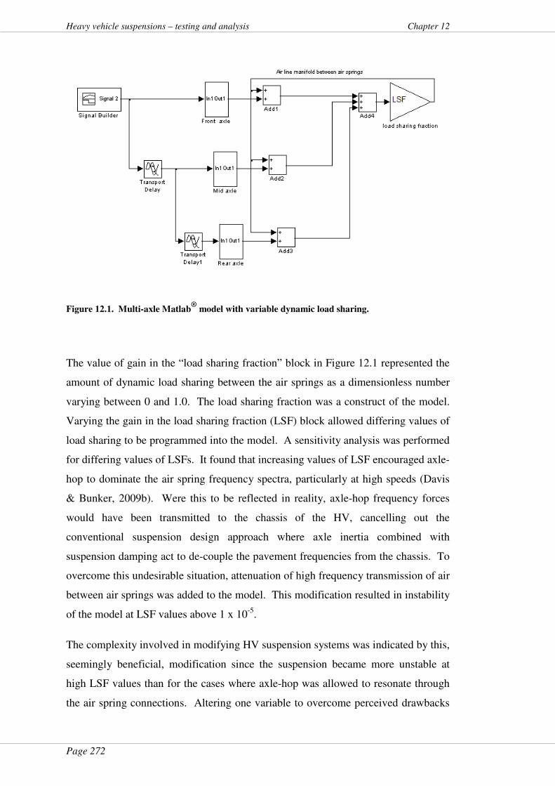
Page 272
Heavy vehicle suspensions – testing and analysis Chapter 12
Figure 12.1. Multi-axle Matlab®
model with variable dynamic load sharing.
The value of gain in the “load sharing fraction” block in Figure 12.1 represented the
amount of dynamic load sharing between the air springs as a dimensionless number
varying between 0 and 1.0. The load sharing fraction was a construct of the model.
Varying the gain in the load sharing fraction (LSF) block allowed differing values of
load sharing to be programmed into the model. A sensitivity analysis was performed
for differing values of LSFs. It found that increasing values of LSF encouraged axle-
hop to dominate the air spring frequency spectra, particularly at high speeds (Davis
& Bunker, 2009b). Were this to be reflected in reality, axle-hop frequency forces
would have been transmitted to the chassis of the HV, cancelling out the
conventional suspension design approach where axle inertia combined with
suspension damping act to de-couple the pavement frequencies from the chassis. To
overcome this undesirable situation, attenuation of high frequency transmission of air
between air springs was added to the model. This modification resulted in instability
of the model at LSF values above 1 x 10⁻⁵.
The complexity involved in modifying HV suspension systems was indicated by this,
seemingly beneficial, modification since the suspension became more unstable at
high LSF values than for the cases where axle-hop was allowed to resonate through
the air spring connections. Altering one variable to overcome perceived drawbacks

Page 273
Chapter 12 Heavy vehicle suspensions – testing and analysis
did not result in improvements to the model in other areas.
The damper characteristics were varied (Davis & Bunker, 2009b) to ones that were
different, but known. The characteristics for the dampers on the coach were
substituted for those in the semi-trailer axle model (Figure 5.13) and then configured
as in Figure 12.1. With this substitution, the model proved stable for LSFs up to 1.0
(i.e. 100 percent transmission of air between air springs). Altering the shock
absorber characteristics allowed the model to maintain stability and have increased
air line sizing. These results indicated that air lines between sequential air springs
could have diameters in the order of those of the air springs themselves, provided the
shock absorber characteristics were more aligned with those found on passenger
coaches. This proposal will be left at that point as it is venturing out-of-scope,
except to refer to Chapter 13, Section 13.3 for potential future research.
12.2.5 Alterations to HV suspension metrics from the use of
larger longitudinal air lines
Objective 2 was met by the use of the innovative approach to correlation coefficients
between air spring forces and wheel forces as well as deriving metrics for different
independent variables such as test speed and “novel roughness” values in Chapter 10.
The results indicated strongly that dynamic load sharing was facilitated at the air
springs of the multi-axle HVs tested with larger longitudinal air lines fitted. Further,
suspension metrics involving peak dynamic forces measured at the air springs were,
in general, reduced somewhat by the use of larger longitudinal air lines. This second
phenomenon was likely due to the presence of a greater volume of compressible fluid
(air) in the larger air lines absorbing peaks in dynamic forces.
Suspension metrics derived from wheel forces did not indicate consistent
improvements from the use of larger longitudinal air lines for the HV tested. It is
suggested that this is due to the limitation of the damper characteristics as explored
briefly in Section 12.2.4 and extensively in other work developed for this project
(Davis & Bunker, 2009b). This latter proposal is mentioned here since the
developers of the larger longitudinal air line system tested for this project, properly,
did not alter the damper characteristics on the HVs tested. To do so would have
Page 274
Heavy vehicle suspensions – testing and analysis Chapter 12
invalidated the VSB 11 certification of the axles used. Were such modifications
undertaken, in contravention of suspension certification, potentially more alterations
to wheel and chassis forces may have been made. This will be expanded in Chapter
13 Section 13.3.
12.3 Development of heavy vehicle in-service
suspension testing methods – Objective 3
12.3.1 In-service HV testing
Objective 3 hypothesised that low cost in-service HV suspension testing was
possible. The following two sections outline how that aim was achieved for the
project. This work will be provided to the National Transport Commission (NTC) to
further the progress of the in-service HV suspension testing project.
12.3.2 In-service HV testing – impulse testing
Systems theory (Doebelin, 1980) informs that the perfect impulse of infinitely small
duration contains all frequencies at the same amplitude. The reality falls somewhat
short of this ideal since all impulses are finite. Nonetheless, system characterisation
may be performed by measuring the output of a system after the application of an
imperfect impulse as an input (Chesmond, 1982; Doebelin, 1980). Chapter 6
detailed the results of applying this methodology to heavy vehicle (HV) suspensions
as a system.
The innovative “pipe test” results were compared to those of a VSB 11-style step
test. These were discussed in detail in Chapter 11. The “proof-of-concept” for this
innovative, low cost method was shown to have errors in the order of approximately
16 percent when compared with VSB 11-style test results or manufacturer’s data.
These results were an order of magnitude lower than indicated by other research
(Prem et al., 1998; Uffelmann & Walter, 1994) indicating that the methodology
described herein has contributed an improvement to any proposals for in-service HV
suspension testing.
Page 275
Chapter 12 Heavy vehicle suspensions – testing and analysis
12.3.3 In-service HV testing – roller bed
The roller bed testing results detailed in Chapter 7, Section 7.5 indicated that
dynamic oscillatory excitation to a HV wheel could be used to detect damper health
from wheel forces. The worse the shock absorber condition, the greater the dynamic
range of the wheel force signal measured at the roller. The dynamic wheel force
range for 4 mm excursions approximately doubled when the dampers were removed
compared with the case for new shock absorbers. The trend found in the test results
suggested that even greater dynamic wheel force ranges are being imposed for on-
road excursions larger than 4 mm when HVs are operating with dampers in a
condition where they are wearing tyres abnormally. These results will be
extrapolated in a limited fashion in Section 12.4.2 regarding the additional damage
that worn dampers cause vs. those in healthy HV suspensions.
The project showed that damper condition was detectable using the test unit (Section
3.3) as designed. This “proof-of-concept” experimental design met the requirement
for a low-cost suspension test in that, after approximately $AUD10,000 in set-up
costs, the cost of analysis per axle-group would be approximately $AUD100. The
results indicated that a “proof-of-concept” for a moderate-cost testing machine and
low cost-per-test has been achieved with the use of a modified roller-brake tester.
The brake-testing machine from which the test rig was made was a standard unit that
was not altered with respect to its original overall dimensions. A commercial variant
of it should therefore be able to fit into existing infrastructure at roadside interception
sites or vehicle maintenance facilities where brake testers are designed to fit.
12.4 Implications for network assets
12.4.1 Using tyre wear as an indicator of damper health
The roller bed testing results detailed in Chapter 7, Section 7.5 showed that, for a
damper causing tyre wear, the axle-hop forces were more than 10 percent greater
than for those where the damper was in good condition for excitations using a local
radial reduction of 2 mm in the roller diameter. The analogous forces with a 4 mm
radial shave off the roller were more than 30 percent greater than for those where the
Page 276
Heavy vehicle suspensions – testing and analysis Chapter 12
damper was in good condition.
54 percent of 121 air-sprung HVs surveyed at Marulan, NSW, in 2006 had dampers
that did not meet VSB 11 but did not have apparent tyre wear (Blanksby et al.,
2006). As mentioned in Section 1.4.3, Marulan was not on a HML route at the time;
some anecdotal views have opined that the Marulan results had little relevance since
VSB 11 compliance was not a requirement for operation on that route. That
argument is specious and has been dealt with in Section 1.4.3. The main issue is that
HV suspensions worn to the point where tyre wear is apparent do not meet VSB 11
and therefore impose greater forces than do healthy HV suspensions.
The Australasian Road Transport Suppliers Association (ARTSA) advises, amongst
other activities, the air suspension industry via a code of practice (Australian Road
Transport Suppliers Association, 2001). That document lists (p. 21), under the
heading “shock absorber troubleshooting indicators” the advice that replacement of
shock absorbers should be considered when an “increase in tyre wear and flat spots”
is/are apparent. This advice to use tyre wear as a trigger for damper replacement
needs to be reviewed.
12.4.2 Regarding the community cost of poor HV suspension
health
Costanzi & Cebon (2007; 2005) modelled a fleet of HVs with 50 percent ineffective
dampers. The conclusion from that work was that, at higher mass limits (HML)
loadings, pavement and surfacing damage would be 20 to 30 percent greater than for
a comparable freight task with a fleet equipped with dampers in good condition.
That was for the Newell Highway, which has thicker pavements and surfacings than
the majority of Queensland HML routes (Queensland Department of Main Roads,
2007). Nonetheless, to start an approximate exercise; the Main Roads maintenance
budget in 2008 was AUD$253M (Queensland Department of Main Roads, 2008).
The HML network in Queensland comprises approximately one-third of the road
network. It is not unreasonable to propose that road asset damage is due to heavy
vehicles compared with the damage from any other form of road traffic. On an,
admittedly, broad-brush approximation, the Costanzi & Cebon figures of 20 to 30
Page 277
Chapter 12 Heavy vehicle suspensions – testing and analysis
percent translate into an approximate upper bound of AUD$26M per annum saved
on that portion of the network used at HML loads, were HML HVs to have dampers
maintained across the fleet.
Consider then, the roller bed testing described in Chapter 7, Section 7.5. For that
exercise, 4 mm excitations were successful in deterministic detection of damper
health when axle-hop frequencies were induced into a HV wheel. Previous research
(Davis & Bunker, 2008e) has shown that HV wheel loads at highway speeds resonate
continuously at axle-hop frequencies in the range 10 Hz to 12 Hz. For the case of
worn shock absorbers on the roller bed, the 4 mm excitation at 12 Hz resulted in an
increased peak wheel-load of 70 kg more than for the case for new shock absorbers.
The axle-hop excitation for the case no shock absorbers resulted in a peak wheel load
of 205 kg more than for the case for new shock absorbers.
Let us estimate that, conservatively, road excitation has a 4 mm range (in reality, a
low estimate). Let us choose HVs with worn shock absorbers in condition-states
somewhere between tyre wear being apparent to totally ineffective. The wheel force
increases above static ranging from 70 to 205 kg for that range of condition-states
indicate that peak loadings on pavements and bridges would be between 70 kg (2.3
percent of statutory mass) and 205 kg (6.8 percent of statutory mass) higher than for
the case of well-maintained shock absorbers.
The fourth-power rule has been questioned earlier (section 2.4.2) by many
researchers. Nonetheless, applying this rule allows a comparison with generally
accepted civil engineering lore for the relationship between loadings on granular-
based pavements and pavement damage. Accordingly, the 2.3 percent and 6.8
percent range (above) indicates that instantaneous loading from worn, out-of
specification or defective shock absorbers on HVs would create instantaneous
loading damage increases in the range of 9.7 percent to 30.2 percent when compared
with well-maintained dampers. This range of increased damage due to worn
dampers is similar to the damage increase estimates from the approach developed by
Costanzi & Cebon (2005). It is, however, then able to be extrapolated across the
entire network as the testing in the roller bed testing described in Chapter 7, Section
7.5 was performed at maximum statutory mass wheel loads, not HML.
Page 278
Heavy vehicle suspensions – testing and analysis Chapter 12
This exercise does not account for the twelfth-power rule for concrete pavements;
that exponent would indicate a greater increase in damage, nor does it account for
excitation due to road irregularities or axle-hop values of greater than 4 mm.
12.5 Application of OBM to heavy vehicle mass
monitoring policy – Objective 4
12.5.1 On-board mass system tamper evidence and accuracy
Objective 4 was to determine the accuracy and potential for tamper-evidence of on-
board mass (OBM) measurement systems for the purposes of an Australian
regulatory regime. This Objective was met from the results of the testing of OBM
systems detailed in Chapter 8 and Chapter 9. These chapters showed the results of
characterising the available OBM systems in Australia and development of tamper
indicators, including the tamper index (TIX). The following sections address how
these developments may be used for Stage 2 of the Intelligent Access Project.
12.5.2 Tamper metrics
The Intelligent Access Programme (IAP), administered by Transport Certification
Australia and mentioned in Section 1.5.1, has implemented satellite tracking of
heavy vehicles (HVs) (Koniditsiotis, Taylor, Davis et al., 2004). One of the enabling
platforms for this programme is the global navigation satellite system (GNSS),
commonly referred to as the global positioning system4 (GPS). The success and
robustness of the implementation of this tracking under Stage 1 of the IAP has been
by careful specification of multiple quality indicators derived from the GPS output
data. Stage 2 of the IAP will likewise have a strong emphasis on multiple quality
indicators.
Jurisdictions are considering specifying OBM as part of their regulatory frameworks
but require confidence regarding the performance of those systems (Australia
Department of Transport and Regional Services, 2005a, 2005b; Karl et al., 2009).
4Strictly speaking, GPS is a US system; GNSS is the generic term for all satellite navigation systems.
Page 279
Chapter 12 Heavy vehicle suspensions – testing and analysis
The details of such implementation are part of Stage 2 of the Intelligent Access
Program outlined in Section 1.5. Accordingly, one tamper indicator will not be
sufficient to prosecute, or even indicate with certainty, a tampering event. Where a
combination of the scenarios developed in Chapter 9 were apparent, it would be
highly likely that a tamper event had occurred. This approach will be presented to
TCA. This will be in conjunction with arrangements for supply of the tamper
algorithms either developed as part of this project or as part of the ongoing OBM
Stage 2 project under IAP.
12.5.3 Tamper evident specifications
Jurisdictions and transport regulators require OBM solutions (Karl, 2007; Karl et al.,
2009; Karl & Han, 2007) to an evidentiary level (i.e. accurate enough to be used as
evidence in a prosecution). Previous experience with Stage 1 of the IAP was that
more than one quality indicator was required for an evidentiary approach to GPS data
(Koniditsiotis et al., 2004). That experience was also informed by the philosophy
that, where technical monitoring rules were pragmatic and were not a great impost on
HV operators, they were adopted. However, where technical solutions to monitoring
were difficult, costly or complex to implement, “business rules” were adopted
instead. Stage 1 of the IAP has a mix of business and technical rules for its
governance framework.
The testing carried out under Transport Certification Australia’s on-board mass
(OBM) accuracy and tamper-evidence programme provided a considerable amount
of data. From the results shown in Chapter 9, dynamic data, amongst other
indicators, will be required to derive robust tamper evidence for OBM systems for
IAP Stage 2. Both frequency-domain and algorithmic approaches to dynamic data
proved useful indicators of tamper events. It appears feasible that tamper detection
may be implemented using logical rule sets and some simple algorithms, most of
which are in the public domain. The example of the GPS data indicating movement
without matching frequency data would be an example of a business rule; the tamper
index (TIX) metric would be an example of a technical rule.
The issue of applying the TIX algorithm developed to detect tampering (Chapter 9)

Page 280
Heavy vehicle suspensions – testing and analysis Chapter 12
to load cell data needs to be addressed. This is because HVs use load cells as well as
APTs to determine OBM readings. The issue of tampering with load cells in the
static environment has been shown to be of concern (Karl et al., 2009b). The TIX
algorithm has not yet been validated against corrupted vs. typical load cell data. A
modified OBM reference system will need to be used to measure dynamic signals
from load cells, before and after they have been wedged, to explore further the
validity of the tampering algorithms and any supporting technical and business rules
developed.
12.5.4 Sampling frequency for OBM systems
The sampling frequency of the reference OBM unit used (Chapter 3, Section 3.4.2)
was 41.6 Hz. The axle-hop frequencies of the HVs tested would very likely be in the
range 10 to 15 Hz and not more than 15 Hz (Cebon, 1999; de Pont, 1997). The
Nyquist sampling criterion (Shannon’s theorem, Section 2.3.3) indicates that the
frequency of sampling needs to be at least twice that of the frequency of the signal of
interest. Accordingly, the dynamic data recorded during the tamper vs. non-tamper
events had a frequency range that was detectable up to approximately 20 Hz (i.e. half
of 41.6 Hz). The derivation of the algorithms in Chapter 9 was predicated on data
with that frequency range.
Assuming that OBM is implemented under Stage 2 of the IAP and that tamper-
evident rules are applied similar to those developed in Chapter 9. Those rules were
validated using data containing axle-hop frequencies. For those rules to be
successful, the dynamic data from the OBM systems in the field will need to have a
similar frequency range to that used for development of those rules in this chapter,
i.e. more than twice any axle-hop frequency. Hence, the sampling frequency of the
OBM units in the field under IAP Stage 2 will need to be at least 30 Hz, otherwise
additional testing will need to be undertaken to validate other algorithms to those
developed for this project. This conclusion has implications for OBM manufacturers
in Australia.
Most OBM systems do not sample at frequencies capable of detecting axle-hop.
Indeed, most do not sample at frequencies capable of detecting body bounce, which

Page 281
Chapter 12 Heavy vehicle suspensions – testing and analysis
would require a maximum sampling frequency of approximately 5 Hz (Davis, 2008).
There are a number of reasons for this limitation within OBM units. One is to keep
costs down, since the cost of an electronic chip is related to its sample rate; higher
sample rate, higher cost. Another reason is that lower sample rates do not require
much buffering of the final OBM readout to stop display jitter. Higher primary
transducer data sample rates will require more buffering than used at present. Were
the same buffering to be used as at present but with higher sample rates, OBM
displays would jitter due to inherent noise and the digitisation indeterminacy within
all electronic systems. Accordingly, as implemented at the time of writing, the
majority of OBM manufacturers choose low sample rates for their equipment to keep
buffer and sampling chip costs down (Davis, 2008). Both the use of dynamic signals
from the OBM units for the tamper index (TIX) metric and business rules regarding
movement of the vehicle compared with dynamic data will need to be considered as
Transport Certification Australia moves into the specification phase for the OBM
feasibility project.
12.5.5 Load cell tampering
Anecdotal data had it that wedges may be inserted under load cells resulting in the
reading from the load cell indicating less than the actual applied load (Davis, 2008).
The OBM test programme showed that view to be the case (Karl et al., 2009b).
The issue of using dynamic data to detect load cell tampering has yet to be
determined. This was due to the inability of the load cells, where they were the
primary OBM transducers, to be connected to both the dynamic reference system and
the test OBM system simultaneously during the OBM test programme. Parallel
verification of primary transducer signals via the reference OBM system vs. the test
OBM system was the aim of the test programme as designed. This arrangement
could not be implemented for the load cell cases, due to their inability to be
connected to two measurement devices at once. This limitation, imposed by the
physics of the load cell bridges, meant that load cell dynamic signals were not
measured during the OBM testing. However, dynamic data have been recorded from
load cells during other testing (Davis & Sack, 2005). An example of the frequency
signature of load cell dynamic data, in the form of the FFT of data recorded from the
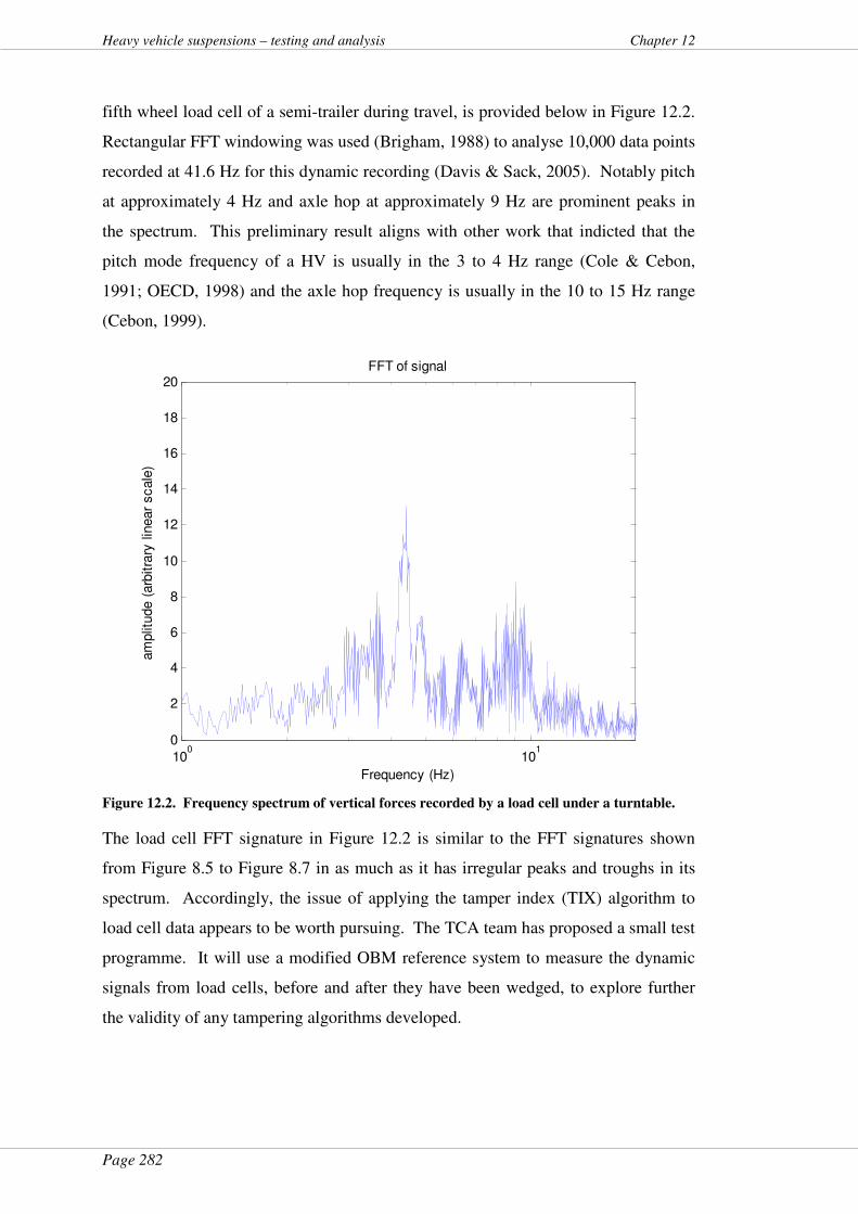
Page 282
Heavy vehicle suspensions – testing and analysis Chapter 12
fifth wheel load cell of a semi-trailer during travel, is provided below in Figure 12.2.
Rectangular FFT windowing was used (Brigham, 1988) to analyse 10,000 data points
recorded at 41.6 Hz for this dynamic recording (Davis & Sack, 2005). Notably pitch
at approximately 4 Hz and axle hop at approximately 9 Hz are prominent peaks in
the spectrum. This preliminary result aligns with other work that indicted that the
pitch mode frequency of a HV is usually in the 3 to 4 Hz range (Cole & Cebon,
1991; OECD, 1998) and the axle hop frequency is usually in the 10 to 15 Hz range
(Cebon, 1999).
100
101
0
2
4
6
8
10
12
14
16
18
20FFT of signal
Frequency (Hz)
am
plit
ude (
arb
itra
ry lin
ear
scale
)
Figure 12.2. Frequency spectrum of vertical forces recorded by a load cell under a turntable.
The load cell FFT signature in Figure 12.2 is similar to the FFT signatures shown
from Figure 8.5 to Figure 8.7 in as much as it has irregular peaks and troughs in its
spectrum. Accordingly, the issue of applying the tamper index (TIX) algorithm to
load cell data appears to be worth pursuing. The TCA team has proposed a small test
programme. It will use a modified OBM reference system to measure the dynamic
signals from load cells, before and after they have been wedged, to explore further
the validity of any tampering algorithms developed.
Page 283
Chapter 12 Heavy vehicle suspensions – testing and analysis
12.6 Summary of this chapter
12.6.1 Dynamic load sharing
That dynamic load sharing may be facilitated by larger longitudinal air lines on air-
suspended heavy vehicles (HVs) is indicated strongly by the results in Chapter 10
and discussed further in this chapter. What is not so clear is the potential for
improvements to HV suspension metrics from further increases in dynamic load
sharing. The standard dampers fitted to the semi-trailer axle tested, for example,
appeared to act against further improvements to HV suspension indicators for larger
longitudinal air lines. Conversely, were HV suspension designs to have a holistic
revision which incorporated the increased flow of air between sequential air springs
with a concomitant variation in damper characteristics, even greater reductions in
peak loadings may be possible than those found during this project. This area needs
to be explored by HV designers and the HV manufacturing industry.
12.6.2 In-service HV testing
Chapter 11 outlined some issues and concepts that regulators will need to address to
implement in-service HV suspension testing. This chapter, supported by findings
from Chapter 7, built on those concepts to outline practical methodologies that need
to be considered by the National Transport Commission to implement such testing as
required under the current Queensland and NSW Government funding arrangements
(Australia Department of Transport and Regional Services, 2005a, 2005b).
12.6.3 Community cost of poor HV suspension health
Two indicative exercises on increased instantaneous pavement loadings have been
detailed in Section 12.4.2. The first, applicable to HML routes, indicated a potential
saving of approximately AUD$26M/annum. The second applied the wheel force
values from the roller bed testing described in Chapter 7, Section 7.5. This exercise
indicated that up to approximately 30 percent of the maintenance portion of the
Department of Transport and Main Roads' budget, or approximately
$AUD75M/annum could be gained from the simple expedient of road transport
Page 284
Heavy vehicle suspensions – testing and analysis Chapter 12
operators testing their HVs and replacing worn shock absorbers. This figure is over
and above damage due to overloading; a comment made for future reference but
verging out-of-scope for this project.
It is for noting that this conclusion does not address the community cost of reduction
in HV safety arising from defective, out-of-specification or worn dampers, nor does
it address any Local Government infrastructure costs.
12.6.4 On-board mass systems on heavy vehicles – sampling
rates and synergy with other requirements
The testing of on-board mass (OBM) systems for HVs under this project indicated
certain accuracy and evidentiary levels for OBM systems available in Australia. The
results of these tests (Karl et al., 2009b), to be considered for use in Stage 2 of the
Intelligent Access Project, will be presented to road transport regulators in Australia.
The tamper algorithms developed as part of this project or alternatives created under
other, on-going development arrangements with Transport and Main Roads, will be
presented to Transport Certification Australia’s OBM Stage 2 project under IAP.
The implications for the OBM industry in Australia will be that higher sampling
frequencies than those currently deployed at the primary transducer level will be
required to implement a robust and tamper-evident platform for implementing OBM
monitoring using the algorithms developed during this project or other methods
based on analysis of dynamic data from OBM systems.
Higher sample rates would also facilitate the recording of air spring transients should
the HV traverse a discontinuity. This could facilitate the derivation of suspension
damping characteristics within an in-service HV suspension testing regime. Some
OBM manufacturers already use an accelerometer in an OBM unit to detect the angle
of the HV stance where it is not on level ground. Recording the accelerometer data
during a similar traverse over a discontinuity to that postulated above could be used
to determine suspension health for a different approach, but similar outcome, to
implementation of in-service HV suspension testing.
Page 285
Chapter 12 Heavy vehicle suspensions – testing and analysis
12.7 Conclusions from this chapter
The following list condenses the future industrial research directions from this
project:
1. alter current damping characteristics of commercial shock
absorbers, in conjunction with larger longitudinal air lines, to
improve dynamic load sharing;
2. investigate improvements to suspension metrics from alterations in
1, above;
3. develop a cheap and simple standardised impulse test for air-
suspended HVs with due consideration to the variability of tyre
parameters influencing the results of the tests;
4. measure the error between test data from a standardised impulse test
and VSB 11-certified data for the air suspensions available in
Australia. Circulate to road authorities and implement in-service
suspension testing using an impulse into air suspended HVs;
5. develop a standardised roller bed test for air-suspended HVs;
6. measure the error between test data from a standardised roller bed
test and VSB 11-certified data for the air suspensions available in
Australia. Circulate to road authorities and implement in-service
suspension testing using a roller bed test on in-service air suspended
HVs;
7. review the advice to transport operators that tyre wear is an
indicator of worn dampers; this point is too late in the maintenance
cycle to keep the dampers within specification;
8. specify a minimum of 30 Hz as the sample rate for any on-board
mass system for HVs (suggest 40 Hz to provide a margin for future
applications requiring analysis of HV frequencies above 15 Hz);
9. use OBM systems to measure suspension health after application of
Page 286
Heavy vehicle suspensions – testing and analysis Chapter 12
a standardised impulse under 3, above; and
10. use a modified OBM system to measure dynamic signals from load
cells, before and after tampering, to explore further the validity of
tampering algorithms.
“Opportunity is missed by most people because it is dressed in overalls and looks
like work.” - Thomas Edison.
Page 287
Chapter 13 Heavy vehicle suspensions – testing and analysis
13 Contribution to knowledge – theory and
future work
13.1 About this chapter
Avenues of research and other work have been discovered as the joint project entitled
Heavy vehicle suspensions – testing and analysis has progressed. Those central to
the Objectives (and some others) have been included in this thesis. Other areas of
investigation have led to the conclusion that, were they to be pursued, they would
have ventured out-of-scope. Nonetheless, it is important to provide some directions
to future researchers where this has happened. This chapter serves that purpose.
13.2 Application of heavy vehicle in-service
suspension testing
13.2.1 Future research into the “pipe test” as a low-cost in-
service suspension test
To calibrate the “pipe test” against Vehicle Standards Bulletin (VSB) 11, research
will be needed to determine the characteristics of available suspensions. VSB 11-
compliant suspension models available in Australia in “as new condition” would
need to be matched and documented against some form of standardised in-service or
field impulse test. The margins between the field test results and the VSB 11
characteristics could be noted and distributed, as agreed by regulators. Such a
programme would be the subject of further work in the regulatory field. The results
of some of the background work from this project (Davis, Kel, & Sack, 2007) as well
as the body of work on the “pipe test” herein, as a “proof-of-concept” (and allowing
for the finite resources of this project), should be applied to the issue of testing the
health of suspensions on HVs with steel suspensions by the use of attaching an
accelerometer to their chassis. Other areas of research would be into the alteration of
measured suspension parameters by variations in tyre characteristics such as inflation
pressure, tyre construction, tyre configuration (dual/single), size, tread depth and
case design as these will influence the phenomenon of tyre enveloping and its effect
on the forcing function provided by the pipe test. It is also noted that variations in

Page 288
Heavy vehicle suspensions – testing and analysis Chapter 13
tyre characteristics and tyre enveloping influencing derived suspension parameters
for VSB 11-approved forcing functions are not addressed in VSB 11; a potential
additional avenue for future research.
Chapter 6, Section 6.3 detailed the results for the testing of the semi-trailer and the
coach when subjected to the “pipe test” as a forcing function. The traverse speeds
were too great to elicit a second-order (Section 4.3.1) response that was analysable
for damping ratio. The coach axle responses were analysed in other work leading to
this project (Davis et al., 2007). The tag axle and the drive axle were not able to be
distinguished from examination of the air spring data. This was likely due, as
mentioned in Section 6.4.1, to close coupling of the tag axle and the drive axle within
the same group. Such groups with dissimilar axles make up a small minority of the
heavy vehicle (HV) fleet. Any low-cost test programme developed under the
National Transport Commission in-service HV suspension testing project (Section
1.4) need not be stalled based on the perfect being the enemy of the good.
Nonetheless, further research into low-cost testing for dissimilar axles will need to be
considered given the anomalous results for the coach rear axle group in the testing
described in Chapter 6.
13.2.2 Future research into in-service HV testing – roller bed
The roller bed testing results detailed in Chapter 7, Section 7.5 indicated that
dynamic oscillatory excitation to a HV wheel could detect damper health from wheel
forces. Given that the numbers of HV suspension models available in Australia
certified to VSB 11 are finite (Australia Department of Transport and Regional
Services, 2004b), all available models could be subject to roller bed testing similar to
that undertaken in Chapter 7, Section 7.5. The results for these could be correlated,
documented and referenced against “as new” certified VSB 11 values and then
known values of degradation of suspension dampers and corresponding decay in
VSB 11 parameters, particularly in the critically important damping ratio (Section
11.4.1) plotted over time.
Page 289
Chapter 13 Heavy vehicle suspensions – testing and analysis
13.3 Future research into dynamic load sharing
13.3.1 Future research into improvements dynamic load
sharing by use of larger longitudinal air lines
It is venturing outside the scope of the Heavy vehicle suspensions – testing and
analysis project to explore the fluid mechanics of airflow between air springs.
However, a few points may be central to future research in this area:
� the comparison of wheel and suspension forces for standard vs.
larger longitudinal air lines between air springs has been
documented (Davis, 2006a, 2007; Davis & Bunker, 2008d; Davis &
Bunker, 2008e; Davis & Kel, 2007);
� the nature of improved air flow between air springs using larger
longitudinal air lines has been addressed (Li & McLean, 2003a,
2003b; McLean, Lambert, & Haire, 2001) with research continuing;
and
� the Li and McLean (2003b) study postulated an improvement of 22
times greater air flow between air springs for 20 mm diameter air
pipes vs. 4.15 mm diameter pipes.
The frequency spectra of the larger longitudinal air lines used in the "Haire
suspension system" did not move radically into axle-hop (Davis & Bunker, 2008e)
during “live-drive” testing. That is, the modification did not result in instability or
increase in axle-hop during actual testing. This was borne out by analysis of the data
for this project (Davis & Bunker, 2008e). Mapping this result to the model used in
Chapter 12, Section 12.2.4, leads to the conclusion that the longitudinal air line
diameter modification did not result in a corresponding model load sharing factor
(LSF) any greater than an order-of-magnitude of approximately 1 x 10⁻⁶ (i.e. an
order-of magnitude below 1 x 10⁻⁵).
If the smaller air lines have flows 22 times less than 20 mm air lines (the size of the
connectors used in the “Haire suspension system”), this concept indicates that their
LSFs are in the order of magnitude of sub-1 x10⁻⁷. Further, given that body bounce
for the test case where the "Haire suspension system" was fitted did not result in
Page 290
Heavy vehicle suspensions – testing and analysis Chapter 13
vehicle instability, it is reasonable to infer that this system extracts the benefits of
speedier transfer of air between successive air springs without the potential for
instability arising from low-frequency runaway. The issue of suspension dampers
needs to be addressed in light of the findings of Chapter 12, Section 12.2.4 and other
work within this project (Davis & Bunker, 2009b). Those approaches indicated that
increased dynamic load sharing is being hampered by the characteristics of the
standard dampers on the axles of (say) the semi-trailer tested. This since altering the
damper characteristics in the suspension model to those from another, known,
suspension resulted in reduced transmission of axle-hop, no instability at high speed
and extremely low restriction in air flow between air springs.
The industry behind the supply of HVs should consider more research into providing
better load sharing than found currently in most HV suspensions. Societal benefits
accruing from reductions in peak loadings leading to reduced road damage, reduced
payload damage (especially for fragile goods), less fatigued drivers and passengers,
and greater life from heavy vehicle chassis, suspension and coachwork components
may be the result.
13.3.2 Future research into load sharing metrics
Any improvement to a HV’s dynamic load coefficient (DLC) was shown
mathematically to be mutually exclusive to an improvement to its load sharing
coefficient (LSC) in Section 2.5. The results shown in Sections 10.3.4 and 10.3.5
indicated that this might be the case for the two multi-axle HVs tested. With the
exception of the tag axle wheel forces, the LSC did not improve when the DLC did
and vice versa for the two cases tested. Further research should be undertaken on
this issue since both the LSC and the DLC have been used extensively over the past
few decades as measures of HV suspension effectiveness (Davis & Bunker, 2007).
Page 291
Chapter 13 Heavy vehicle suspensions – testing and analysis
13.4 Wheel forces within pavement damage models
Three HVs were tested as described in Chapter 3, Section 3.2. The data from those
tests were used in Chapter 7, Section 7.3 Section 7.4 to show derived wheel forces
against a “novel roughness” measure and against test speed. When checked for
statistical significance, mean wheels forces varied per side for the bus and the semi-
trailer. This appeared to be the result of the effect of the cross-fall of the road
shifting the HVs’ centres-of-gravity to the left or the right and the ability of the
heavy vehicle (HV) to compensate for this action.
The bus wheel force standard deviations, mean wheel forces and peak wheel forces
did not correlate to increasing “novel roughness” values. Neither did the coach and
semi-trailer wheel force standard deviations and mean wheel forces correlate with
increasing “novel roughness” values. However, peak wheel forces from the coach
and the semi-trailer did correlate to increasing values in “novel roughness”.
Left/right variations were evident in peak and mean wheel forces derived from the
bus over the range of “novel roughness” values. Only mean wheel forces varied per
side for the coach and the semi-trailer in the same variable-space.
Indicatively, the semi-trailer exhibited variation per side in mean wheel forces both
per test speed and per “novel roughness” value. Peak forces for the bus and the
coach did not. By using data per test speed instead of roughness, different results
were obtained for the derived parameters. These results were from the same data
sets. Care needs to be exercised, therefore, in ensuring that results from one method
are cross checked against results from another method.
As noted in Chapter 2, pavement damage models use a “power law” damage
exponent to attempt to account for the variation in empirical pavement life correlated
to axle passes. A single pass from an axle that does not bounce causes rutting and
has a damage exponent tending to 1.0 (de Pont & Steven, 1999). To “build in” an
allowance for dynamic wheel forces, damage exponents ranging from 1.0 to 12 are
used (Austroads, 1992; Pidwerbesky, 1989). These approaches to pavement damage
models need to be considered in terms of these results. In particular, the left/right
variation apparent in mean wheel forces and the highly-dependent relationship
between “novel roughness” values and peak wheel forces needs to be investigated
Page 292
Heavy vehicle suspensions – testing and analysis Chapter 13
further by pavement technologists, geotechnical engineers, and other domain experts.
This particularly for the pavement peak loading issue and left/right variations. This
latter particularly indicating that the pavement under the outer wheel path should
have a different design standard from that of the inner wheel path pavement.
Augmentation of pavement models needs to account for dynamic wheel loading
effects now that the dynamic data for HV wheel forces from this project have been
documented. This augmentation needs to take into account a more complex set of
considerations than simply the peak forces or the static loads. Chapter 2 detailed
some pavement damage models that used static load values. The results in Chapter 7
indicated that the mean wheel forces might be indicated by static loads. However,
the on-board mass portion of this project found that mean wheel forces are not equal
to static wheel forces (Karl et al., 2009b). Further, neither roughness values nor peak
wheel forces are included in any Australian pavement design model (Austroads,
1992; Main Roads Western Australia, 2005; Moffatt, 2008). The results in Chapter 7
indicated that the correlation of wheel forces to roughness needs to be explored
further, with this concept being noted in other research (OECD, 1992, 1998).
Further, the adherence to HV suspension dynamic metrics containing only standard
deviations (Eisenmann, 1975; Sweatman, 1983) needs to be re-examined since peak
wheel forces of the most common line-haul HV in Australia varied proportional to
“novel roughness” in a statistically significant manner whereas neither the wheel
force standard deviations nor the mean wheel forces so varied.
13.5 Suspension wavelength and the HV fleet
Chapter 7, Section 7.4 showed indicative fast Fourier transform (FFT) plots of peak
wheel forces. In these, the contribution that body bounce forces made to pavement
forces was shown to be approximately equal in magnitude to that of axle-hop forces.
Accordingly, two sets of suspension wavelengths need to be examined as they both
contribute approximately equally to instantaneous pavement forces from HV wheels.
The results shown in Chapter 7, Section 7.4 indicated that wheel forces from body
bounce at highway speeds would be repeated at approximately 15 to 28 m spacings5.
5 27.7m for 10Hz and 100km/h
Page 293
Chapter 13 Heavy vehicle suspensions – testing and analysis
Axle-hop repetitive forces will occur at approximately 2 to 2.5 m intervals,
depending on speed of travel. These effects are termed “spatial repetition” and have
been well documented (Cole & Cebon, 1992; Cole et al., 1996; Collop et al., 1996;
Collop et al., 1994; Jacob, 1996; LeBlanc & Woodrooffe, 1995).
Should a particular suspension have its axle-hop frequency (i.e. axle-hop force
repetition) as a multiple of its body bounce frequency, an approximate doubling of
the instantaneous pavement force will occur where the two coincide at a common
wavelength node. Pavement distress will then be concentrated as a patch at that
point with damage proportional to a suitable exponent.
The Australian road transport network has been opened up to increasing numbers of
HML vehicles and lengths of road declared HML routes. With this increase, there
has been a concomitant number of HVs fitted with RFS. Accordingly, the
suspension characteristics of the HV fleet have become more homogenous than in
the past. This then provides for a continuing homogenisation of HV suspension
characteristics, particularly with respect to body bounce frequencies, namely:
� more highly correlated wheel forces from the heavy vehicle fleet;
� pavement distress likely concentrated in patches distributed
longitudinally; and
� that concentration to predominate at intervals of approximately 15
to 30 m for highway segments, particularly those with laden semi-
trailer traffic.
That spatial repetition would need to be addressed eventually had been foreseen
(LeBlanc, 1995). The results from this project agree with that proposition. There is
a need for research into the effects of mandated uniform HV suspension
characteristics and that is now more urgent than when first mooted by researchers
such as LeBlanc (1995) about 15 years ago. Where the body bounce wavelength of a
HV suspension creates a maximum instantaneous force at a point on a pavement and
the axle-hop forces are coincidental at that point, a potential doubling of the
instantaneous wheel forces will likely occur, especially at highway speeds. Hence
distress points at 25 m intervals would be expected, coincident with distress points at
Page 294
Heavy vehicle suspensions – testing and analysis Chapter 13
2.5 m intervals caused by HVs with homogeneous suspensions all bouncing at or
below 2 Hz.
The measures of standard deviation, mean and peak dynamic wheel forces combine
to show a picture of pavement forces in the real world. Instantaneous values of these
forces can be up to double those of the static force for which the pavement was
designed. Further, pavement “novel roughness” provides a reasonable indicator of
maximum wheel forces and their range. Wheel force maxima and dynamic range for
three HVs have been determined and documented for this project.
Dynamic pavement forces created by heavy vehicles have been modelled for some
decades. The current pavement models that use a number of quasi-static passes of a
HV axle at a theoretical loading to determine pavement life do not always account
for peak dynamic forces or the variation of those forces around the mean. It is the
peak (within the upper tail) of wheel loads that do the damage, however, whether or
not an empirical “power law” is applied. The quasi-static application of pavement
loads from HV wheel forces in traditional models for pavement design needs to be
reviewed to incorporate the dynamic data from the research presented here and by
others. This especially since the regulatory system and the pavement design process
both define static wheel forces as the determining factor for HV impacts. Clearly,
this measure has little value when the dynamic pavement loads from HVs are
understood.
13.6 Future directions of research into on-board
mass monitoring of heavy vehicles
13.6.1 Future OBM research
Some significant areas of potential tampering have been addressed in the test
programme; development of both technical and business options to detect these
events will need to be addressed for implementation of regulatory OBM system
application to Australian HVs. Agreed best practice guidelines and procedures for
installation, calibration, operation and maintenance will be developed as TCA moves
into the regulatory phase for OBM implementation. The test programme
investigated the potential use of additional intelligence derived from analysis of
Page 295
Chapter 13 Heavy vehicle suspensions – testing and analysis
dynamic OBM data as validation against data from the static data recorded by those
OBM systems.
Vulnerability of mechanical and pneumatic systems to degradation, drift and
tampering will need to be further investigated in order to achieve OBM
implementation in the IAP environment but these issues verge outside the scope of
this thesis.
13.7 Conclusions from this chapter
The following points condense the theoretical research directions identified during
this project:
1. further development of suspension models to better analyse the
process of air transfer between air springs on HVs and improve load
sharing and dynamic performance;
2. development of pavement damage models incorporating peak wheel
forces and left/right variation in wheel forces;
3. development, refinement and adoption of pavement damage models
incorporating spatial repetition adopting the work herein and that of
others (Cebon, 1987; Cole & Cebon, 1992; Cole et al., 1996;
Collop, Cebon, & Cole, 1996; Collop et al., 1994; LeBlanc &
Woodrooffe, 1995); and
4. investigation of the susceptibility of HV on-board mass telematic
components to degradation, drift and tampering, and the design
parameters of OBM systems to give greater flexibility for future
applications.
“A prophet is not without honour, save in his own country, and in his own house.” -
Matthew xiii, 57.
Page 296
Heavy vehicle suspensions – testing and analysis Chapter 14
14 Conclusions
14.1 Introduction
This research had a number of objectives. They concerned development of low-cost
in-service heavy vehicle (HV) suspension testing, the effects of large longitudinal air
lines and characteristics of on-board mass (OBM) systems for HVs. Whilst those
objectives may appear to be disparate, they were all centred on measurement of HV
suspension behaviours with the ultimate purpose of reducing the damage and repair
costs to Australian road network assets. This chapter presents the main conclusions
of the study in relation to the Objectives presented in Chapter 1 and as met in the
subsequent chapters. The appropriate areas of research and the results therefrom will
be presented to the various project management groups where their role is applicable
to research carried out in undertaking this project and writing this thesis.
Chapter 2 presented a summary of the HV suspension metrics found in the literature
review for this project (Davis & Bunker, 2007) as well as literature released since
that search.
Chapter 3 presented the details of the experimental procedures used to gather data
for the project as well as the rationale behind the choices of instrumentation and
methodologies used.
Chapter 4 developed some abstract models of HV suspensions. These were used
later in Chapters 5 and 6 with respect to in-service suspension testing. The model
for the semi-trailer was also used later in Chapter 12 to indicate the potential for,
and future directions of research into, implementation of large longitudinal air lines
for HVs.
Chapter 7 analysed wheel forces from the “live-drive” data as described in Chapter
3 as well as the roller bed testing. The wheel force data were developed into “novel
roughness” measures derived from the wheels of each test HV and used in Chapter
10 for determination of dynamic load sharing. The wheel force data were also
analysed and presented in Chapter 7 for left/right variations and for different speeds.
This led on to some conclusions regarding suspension and wheel force frequencies,
their transmission to the pavement and repetitive wheel loads in the spatial domain.
Page 297
Chapter 14 Heavy vehicle suspensions – testing and analysis
The data from the roller-bed testing, gathered as described in Chapter 3, were
analysed as presented in Chapter 7 to inform one part of the in-service suspension
testing portion of the project that was taken up in Chapters 11, 12 and 13.
Chapters 8 and 9 were concerned with the OBM accuracy testing and tamper
evidence portions of the project. These areas documented the first public results of a
programme to test all available OBM systems in a country anywhere in the world.
These results were not stand-alone, however. They also served to inform portions of
the discussion on in-service suspension testing in Chapters 11 and 12.
Chapter 11 was concerned with the technical and policy issues regarding in-service
suspension testing for HVs as informed by this project.
Chapters 12 and 13 together outlined some future directions for theoretical,
regulatory and industrial research that were identified from the work over the course
of the project but which, if pursued, would have taken those portions of the project
out of scope.
14.2 Main conclusions
14.2.1 General
The project objectives were presented in Chapter 1, Section 1.7. These are repeated
below with an accompanying discussion on the results from each. The applicable
chapters of the thesis are cross referenced as sub-headings under each Objective and
within that discussion. Reference to Chapter 1, Figure 1.4, shows the
interconnection of the chapters and provides guidance on how the subject of each
chapter is related to the other chapter subjects. The cross references to the chapters
in the following sections are not sequential due to the fundamental
interconnectedness of the subject matter and the parallel development of different
models as the project proceeded.
Page 298
Heavy vehicle suspensions – testing and analysis Chapter 14
14.3 Objective 1
14.3.1 Dynamic load sharing 1
“Develop at least one dynamic load sharing measure that can be applied to the axle
group, consecutive axles or to consecutive wheels and for more than two axles or
wheels.”
Chapter 2, Sections 2.3.5 and 2.3.8 documented load sharing suspension metrics
applicable to this thesis, their merits and drawbacks discovered during the literature
review. Chapter 2, Section 2.5 explored the relationship that the load sharing
coefficient (LSC) has with the dynamic load coefficient (DLC) and determined that
they were inversely proportional to each other. Chapter 3, Section 3.2.2 detailed the
experimental design and implementation of the testing of three heavy vehicles. An
interesting approach to determining wheel forces was developed in Chapter 7,
Section 7.3.1 which led the development of an independent variable, “novel
roughness” as measured at the wheels of each of the test vehicles.
The dynamic load sharing coefficient (DLSC), as developed by de Pont (de Pont,
1997), was derived from the data collected from the testing outlined in Chapter 3,
Section 3.2.2. These results were used in Chapter 10 to show that the DLSC was
improved at the air springs of the two multi-axle HVs, in a statistically significant
manner, by the use of large longitudinal air lines (i.e. the test case). This
improvement was consistent across all “novel roughness” bands. The wheel force
DLSC was not altered consistently across all “novel roughness” bands for the test
cases, however. That the DLSC was improved at the air springs was shown to be
statistically significant for all “novel roughness” bands. The DLSC was improved
for the test cases of the larger longitudinal air lines at the coach wheels only for low
“novel roughness” (low air line flow events). These were the outcomes of
application of the DLSC as a mature methodology.
An improved method of determining dynamic load sharing was then applied to the
wheel forces and to the air spring forces. This method comprised cross correlation of
forces between wheels and between air springs to determine whether dynamic load
sharing was occurring and, if so, whether the larger longitudinal air lines had made a
statistically significant improvement. The DLSC results indicated that dynamic load

Page 299
Chapter 14 Heavy vehicle suspensions – testing and analysis
sharing was occurring at the air springs for all test cases but at the wheels of the
coach for low air line flow events only. To validate the improved method, the
correlation coefficients from the air springs and the wheel forces were plotted against
HV test speeds. The results indicated that dynamic load sharing was improved at the
air springs, but only at low “novel roughnesses” (low air flow events) at the coach
wheels, by their use. This was the same result as for the application of DLSC and
therefore validated the improved methodology using correlation of forces.
Determining the extent of dynamic load sharing using the correlation coefficient
between two elements of a HV was the first time that this method had been used on a
HV for a test case vs. a control case for two different sized air lines. This was in
accordance, however, with the scientific method of altering one variable at a time
(Mill, 1872). It is submitted that Objective 1 was met.
14.4 Objective 2
14.4.1 Dynamic load sharing 2
“Determine if large air lines on air sprung HVs make a difference to wheel forces
and axle-to-body forces and, if so, determine the quantum of such alterations from
the use of larger longitudinal air lines.”
Chapter 3, Section 3.2.2 detailed the gathering of data during on-road testing of
three instrumented HVs. These HVs were configured such that small (4 mm to 12
mm diameter), “industry-standard” longitudinal air lines could be interchanged with
larger (50 mm diameter proper with 20 mm diameter connectors) longitudinal air
lines: the “Haire suspension system”. This allowed comparison of the forces at the
air spring and the wheels for the control case of small air lines vs. the use of larger
longitudinal air lines. Chapter 10 detailed the results of the analysis of that data
using some mature suspension metrics detailed in Chapter 2. This approach
concluded that there were statistically significant improvements to some suspension
metrics with the use of larger longitudinal air lines, but not in a uniform manner. Of
note were improvements to suspension metrics involving peak dynamic forces
ranging from below the error margin to approximately 24 percent. However, this
Page 300
Heavy vehicle suspensions – testing and analysis Chapter 14
range of improvement was not consistent across all air springs, wheels, roughness
bands or speeds.
The suspension metric that was improved consistently across all air springs for all
roughness bands and all test speeds was the improvement in dynamic load sharing
from the use of larger longitudinal air lines. The improvement in dynamic load
sharing coefficient (DLSC) in all cases varied in a statistically significant manner
from approximately 30 percent to 80 percent.
It is submitted that Objective 2 was therefore met.
Software models of the suspensions of the three HVs tested were developed in
Chapter 4, Section 4.3.7 and Chapter 5, Sections 5.5.4, 5.6.4 and 5.7.5. The
software model for the semi-trailer suspension was used in Chapter 11 to inform
future industrial research into the deployment of larger longitudinal air lines on HVs.
Some exploratory excursions into varying damper characteristics with increasing air
transfer between air springs were undertaken in Chapter 11. These led to the
preliminary conclusion that future research into dynamic load sharing would need to
alter currently available shock absorber damping characteristics to accommodate
potential further gains in dynamic load sharing.
14.5 Objective 3
14.5.1 In-service HV suspension testing
“Explore low-cost HV suspension test methods. Evaluate if low-cost HV suspension
test methods can be made equivalent to VSB 11 outcomes for body bounce and
damping ratio. Evaluate the validity, via “proof-of-concept” of the “pipe test”.
Develop a modified roller-brake tester to impart resonant forces into a HV
suspension and, in part, validate previous work on wheel forces from suspensions in
good condition vs. those equipped with poor/worn shock absorbers. Determine, via
“proof-of-concept”, that a modified roller-brake tester may be used to detect a worn
HV suspension from one within specification. This latter to inform the NTC
project.”
Page 301
Chapter 14 Heavy vehicle suspensions – testing and analysis
Two low-cost methods that may prove useful in developing in-service tests for HV
suspensions were described in Chapter 3, Sections 3.2.3 and 3.3. The results of
these tests were analysed in Chapter 6 and Chapter 7, Section 7.5. The results
indicated that, as a “proof-of-concept”, low-cost HV suspension testing was possible.
The results from the test programme were, at worst, approximately 16 percent in
error from those for the same vehicles tested to Australian specification for “road
friendly” HV suspensions, VSB 11 (Australia Department of Transport and Regional
Services, 2004a). The roller bed testing showed that varying degrees of damper
degradation were detectable from the wheel forces at the roller bearings. These
results have been communicated to the in-service HV suspension testing project staff
at the National Transport Commission. It is submitted that Objective 3 was therefore
met.
The results in Chapter 6 and Chapter 7, Section 7.5 informed a discussion on the
implications of in-service HV suspension testing in Chapter 11, Chapter 12,
Section 12.3 and Chapter 13, Section 13.2.
The results of the quasi-static testing described in Chapter 3, Section 3.2.3 were
used to develop software models of the suspensions of the three HVs tested in
Chapter 4, Section 4.3.7 and Chapter 5, Sections 5.5.4, 5.6.4 and 5.7.5. The model
for the semi-trailer was used in Chapter 11 to inform the future directions of
dynamic load sharing in HVs under Objective 2.
14.6 Objective 4
14.6.1 On-board mass monitoring of HVs – search for
accuracy and tamper-evidence
“Determine the accuracy of currently-available OBM systems. Examine the
accuracy of OBM readings vs. weighbridge readings. Validate the use of dynamic
data from OBM systems to detect tamper events.”
Chapter 1, Section 1.5 outlined the rationale for on-board mass (OBM) systems on
HVs to be deployed as part of Stage 2 of the Intelligent Access Program (IAP).
Chapter 3, Section 3.4 described the data gathering process during the OBM system
Page 302
Heavy vehicle suspensions – testing and analysis Chapter 14
test programme. Chapter 8 presented the analysis of accuracy and linearity of the
OBM systems tested. Chapter 9 described the development of a tamper indicator
and other OBM metrics that could be used by jurisdictions to determine tamper
events.
The results in Chapter 8 indicated that 95 percent of contemporary OBM systems
available in Australia are accurate to +/- 500 kg. When three anomalous results out
of 111 scatter plots of OBM linearity were removed, a total variation of 0.5 percent
in OBM linearity from individual system tests was the result.
Typical deliberate tampering event data from the OBM system testing were analysed
in Chapter 9. A set of tamper indicators was developed in that chapter, including
testing and validation of an algorithm that would indicate a tamper event. This
algorithm, in combination with other logical operations that could be applied to HVs
in the field, was proposed as a way forward for road transport regulators and
jurisdictions in the implementation of OBM systems for HVs.
The application of OBM systems to in-service suspension testing as a crossover
result between objectives from this project (i.e. applicability of OBM to Objective 3)
was broached in Chapter 11, Section 11.3.3. Future directions in OBM research
and industrial applications were developed in Chapter 12, Section 12.5 and
Chapter 13, Section 13.6.
The results in Chapter 8 and Chapter 9 have been presented to jurisdictions for
their judgement on the applicability of OBM to Stage 2 of the IAP (Karl et al.,
2009b). Further, jurisdictions may also now consider other applications of OBM as
part of their regulatory frameworks. It is submitted that Objective 4 was met.
Page 303
Chapter 14 Heavy vehicle suspensions – testing and analysis
“It has always been the fate of those who have made new discoveries to be
disesteemed and slightly spoken of by such as either have had no true relish and
value for the things themselves that are discovered, or have had some prejudice
against the persons by whom the discoveries were made. It would be vain, therefore,
and unreasonable in me to expect to escape the censure of all, or to hope for better
treatment than far worthier persons have met with before me.
But this satisfaction I am sure of having, that the things themselves in the discovery
of which I have been employed are most worthy of our diligent search and inquiry,
being the various and wonderful works of God in different parts of the world; and,
however unfit a person I may be in other respects to have undertaken this task, yet, at
least, I have given a faithful account, and have found some things undiscovered by
any before, and which may at least be some assistance and direction to better
qualified persons who shall come after me.”
- William Dampier.

Page 304
Heavy vehicle suspensions – testing and analysis Appendix 1
Appendix 1 – Instrumentation and calibration of three HVs to
measure wheel force data
Introduction
The following Appendix details the methodology used to derive the values of the
unsprung masses and calibration of axle-mounted strain gauges. The strain gauge
calibration graphs include the correlation of strain gauge readings to wheel forces for
the wheel and the hub jacked off the ground and/or tare and/or full load readings for
the various test vehicles.
Masses outboard of the strain gauges
To find the total dynamic wheel force (Fwheel), the two terms Fshear and ma (Equation
3.1) were derived for the instantaneous data recorded during the tests of the three
HVs in Section 3.2. The unsprung mass m outboard of the strain gauges contributed
the m coefficient of a in the ma term of Equation 3.1. The value of m in Equation
3.1, the unsprung mass outboard of the strain gauges, was found as described below.
In order to determine the masses of the coach and bus axles outboard of the strain
gauges, a bent tag axle and a cracked drive axle housing were procured and cut
through completely at the strain gauge mounting points. These portions of axle were
then weighed on certified scales (Figure A1.1, Figure A1.3, Figure A1.4, and Figure
A1.5). The tag axle was not identical to the one installed on the coach but it was
similar enough to provide a valid mass for this portion of the unsprung mass value.
Unfortunately, a drive axle half-shaft was not available for destruction but a sound
spare was made available on loan. It was weighed and measured. Its mass outside
the strain gauge mounting points was able to be calculated owing to the uniformity of
its shape and by using a standard value for the density of steel (Figure A1.2). The
resultant measurement was added to the measured masses of the wheel/tyre/hub
assembly on the HV tested, the measured mass of the requisite portion of the axle
housing and to the manufacturer’s specified masses (Mack-Volvo, 2007a) for the
other components for the relevant axle/s. This process yielded the value for m (Table
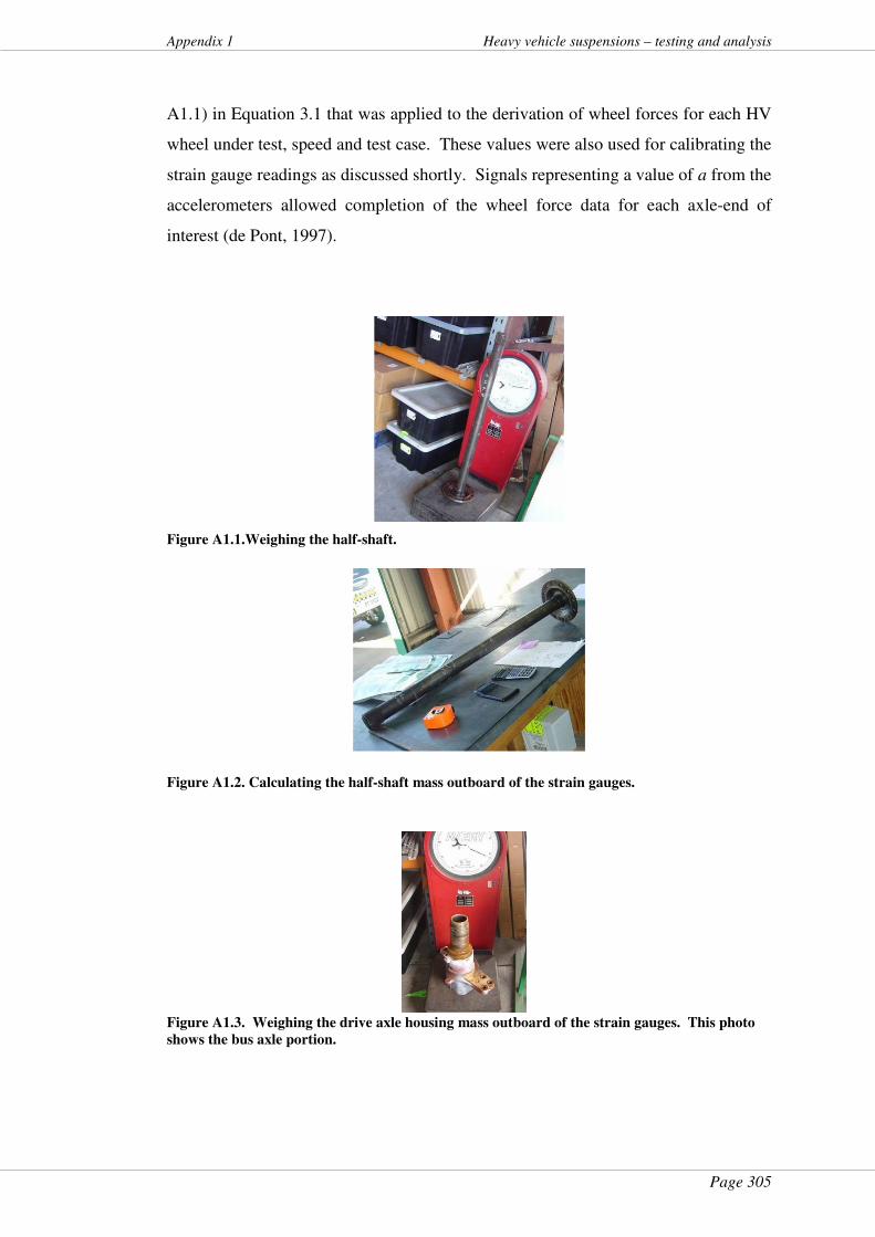
Page 305
Appendix 1 Heavy vehicle suspensions – testing and analysis
A1.1) in Equation 3.1 that was applied to the derivation of wheel forces for each HV
wheel under test, speed and test case. These values were also used for calibrating the
strain gauge readings as discussed shortly. Signals representing a value of a from the
accelerometers allowed completion of the wheel force data for each axle-end of
interest (de Pont, 1997).
Figure A1.1.Weighing the half-shaft.
Figure A1.2. Calculating the half-shaft mass outboard of the strain gauges.
Figure A1.3. Weighing the drive axle housing mass outboard of the strain gauges. This photo
shows the bus axle portion.
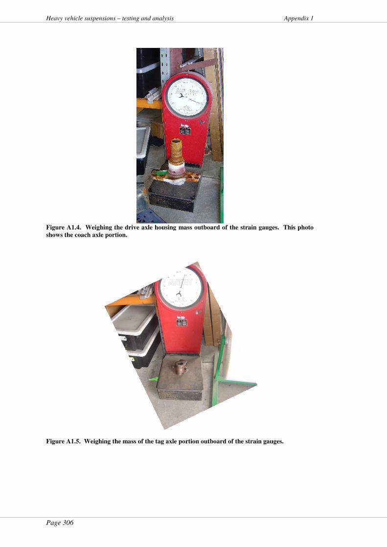
Page 306
Heavy vehicle suspensions – testing and analysis Appendix 1
Figure A1.4. Weighing the drive axle housing mass outboard of the strain gauges. This photo
shows the coach axle portion.
Figure A1.5. Weighing the mass of the tag axle portion outboard of the strain gauges.
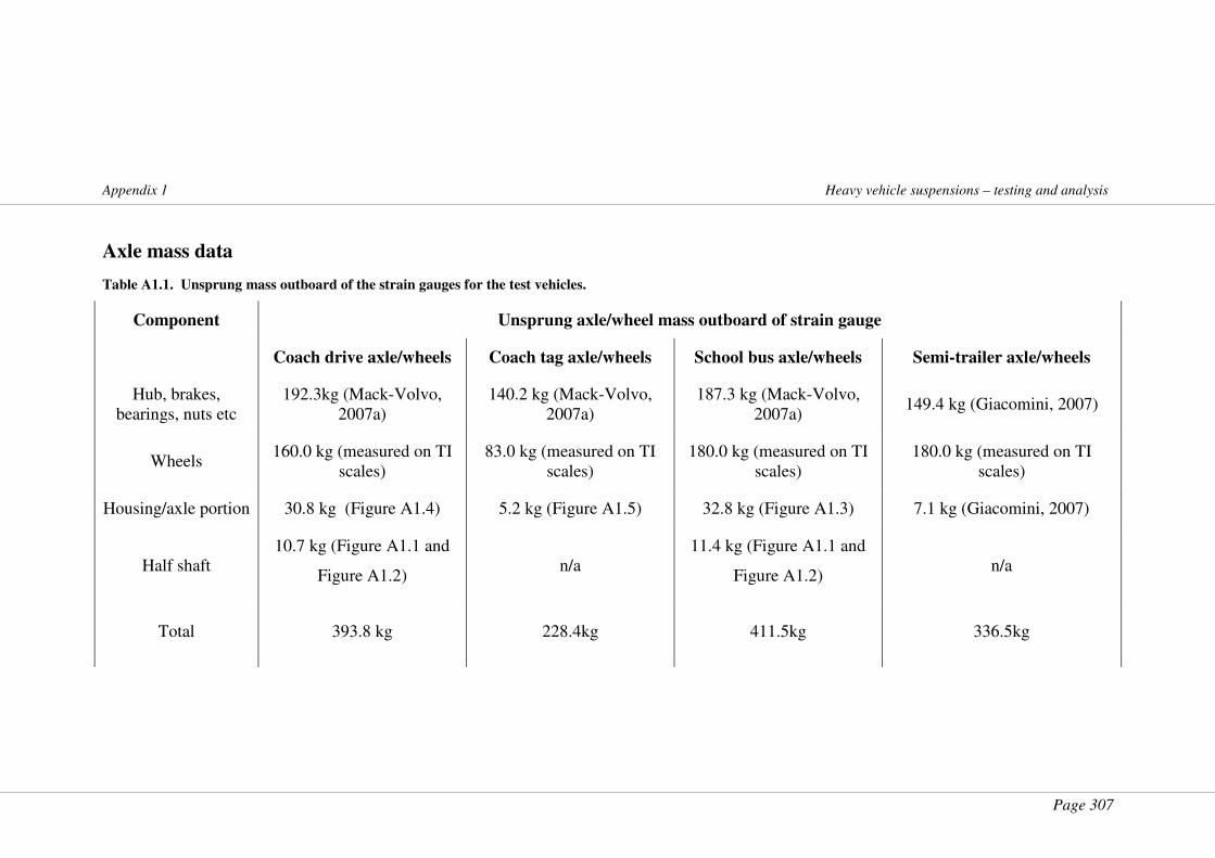
Page 307
Appendix 1 Heavy vehicle suspensions – testing and analysis
Axle mass data
Table A1.1. Unsprung mass outboard of the strain gauges for the test vehicles.
Component Unsprung axle/wheel mass outboard of strain gauge
Coach drive axle/wheels Coach tag axle/wheels School bus axle/wheels Semi-trailer axle/wheels
Hub, brakes, bearings, nuts etc
192.3kg (Mack-Volvo, 2007a)
140.2 kg (Mack-Volvo, 2007a)
187.3 kg (Mack-Volvo, 2007a)
149.4 kg (Giacomini, 2007)
Wheels 160.0 kg (measured on TI
scales) 83.0 kg (measured on TI
scales) 180.0 kg (measured on TI
scales) 180.0 kg (measured on TI
scales)
Housing/axle portion 30.8 kg (Figure A1.4) 5.2 kg (Figure A1.5) 32.8 kg (Figure A1.3) 7.1 kg (Giacomini, 2007)
Half shaft 10.7 kg (Figure A1.1 and
Figure A1.2) n/a
11.4 kg (Figure A1.1 and
Figure A1.2) n/a
Total 393.8 kg 228.4kg 411.5kg 336.5kg

Page 308
Heavy vehicle suspensions – testing and analysis Appendix 1
Calibrating wheel forces vs. axle shear
In order to determine Fshear in Equation 3.1, the relationship between the strain gauge
readings and the forces in the axle resulting from wheel forces needed to be
determined. Accordingly, the Fshear component, measured via strain gauge readings,
was calibrated from its relationship with the wheel force (Woodrooffe et al., 1986) as
follows, with commentary regarding the rationale included in each point:
� the static wheel force exerted by each wheel of the axle group under
test on the test vehicle was measured as a mass from calibrated
scales usually used by transport inspectors for enforcement
purposes. This static mass value was recorded with the test vehicle
on the flat, level floor of an industrial shed. This was done in
conjunction with the calibration of the on-board telemetry system,
for efficiency, after it was installed;
� when static weighing using the scales under each wheel of interest
was undertaken, the static value of Fwheel measured on the scales
contained two force components. These were a static Fshear
component at the strain gauge mounting point inboard of the strain
gauge and acting through the spring; and a static ma force
component. The former due to the mass of the chassis and
suspension components, etc. transmitted via the axle to the wheel;
and the latter a force component due to gravity acting on the
unsprung mass outboard of the strain gauge;
� the measured static wheel force had a constant offset compared with
the strain gauge readings. This margin was the difference between
Fshear and the total force (Fshear + ma); i.e. the latter of the two
components of the static value of Fwheel measured on the scales,
remembering that the strain gauges measured shear proportional
only to the forces inboard of their mounting point;
� to find the constant offset due to the static ma force component, the
chassis of the test vehicles were jacked so that the wheel force
registered as close to zero as possible (+5/-0 kg) on the portable
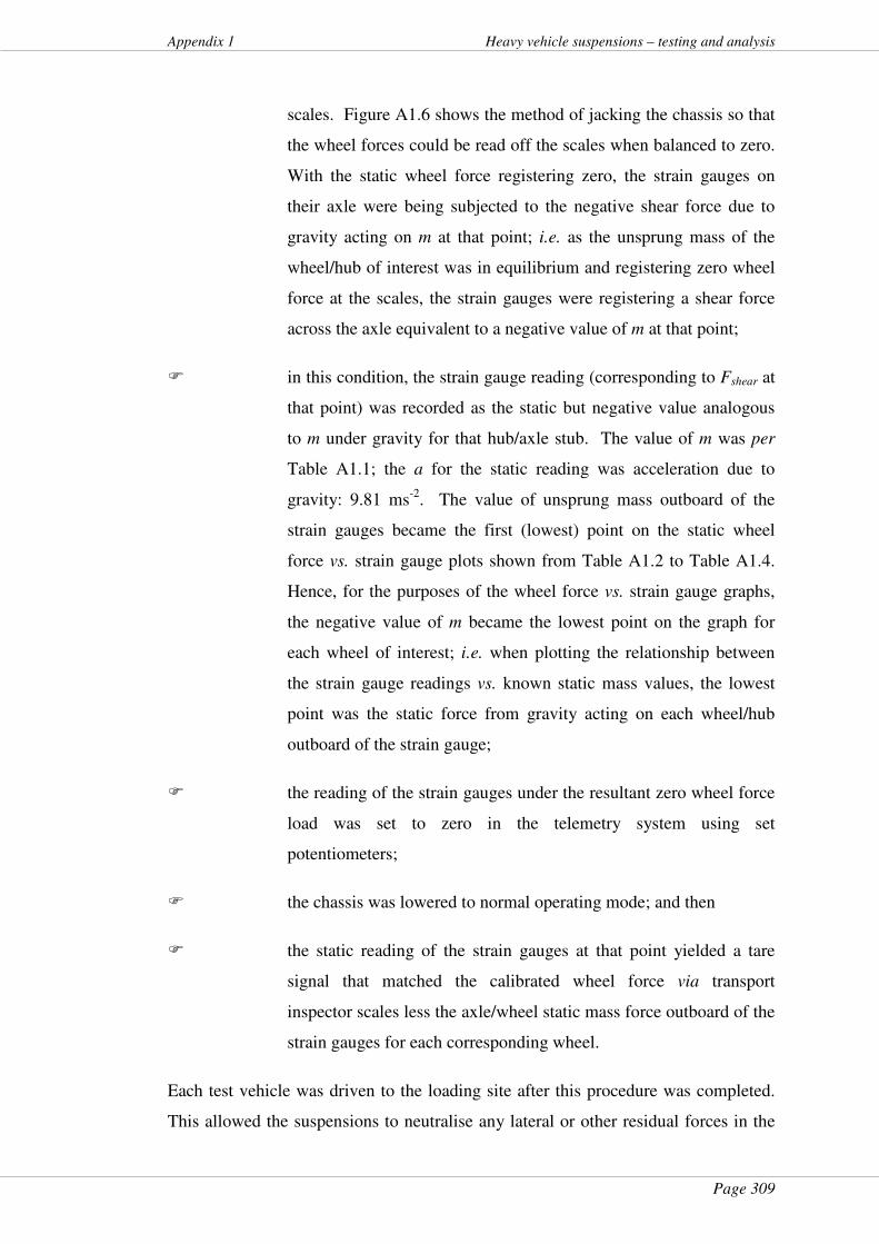
Page 309
Appendix 1 Heavy vehicle suspensions – testing and analysis
scales. Figure A1.6 shows the method of jacking the chassis so that
the wheel forces could be read off the scales when balanced to zero.
With the static wheel force registering zero, the strain gauges on
their axle were being subjected to the negative shear force due to
gravity acting on m at that point; i.e. as the unsprung mass of the
wheel/hub of interest was in equilibrium and registering zero wheel
force at the scales, the strain gauges were registering a shear force
across the axle equivalent to a negative value of m at that point;
� in this condition, the strain gauge reading (corresponding to Fshear at
that point) was recorded as the static but negative value analogous
to m under gravity for that hub/axle stub. The value of m was per
Table A1.1; the a for the static reading was acceleration due to
gravity: 9.81 ms-2. The value of unsprung mass outboard of the
strain gauges became the first (lowest) point on the static wheel
force vs. strain gauge plots shown from Table A1.2 to Table A1.4.
Hence, for the purposes of the wheel force vs. strain gauge graphs,
the negative value of m became the lowest point on the graph for
each wheel of interest; i.e. when plotting the relationship between
the strain gauge readings vs. known static mass values, the lowest
point was the static force from gravity acting on each wheel/hub
outboard of the strain gauge;
� the reading of the strain gauges under the resultant zero wheel force
load was set to zero in the telemetry system using set
potentiometers;
� the chassis was lowered to normal operating mode; and then
� the static reading of the strain gauges at that point yielded a tare
signal that matched the calibrated wheel force via transport
inspector scales less the axle/wheel static mass force outboard of the
strain gauges for each corresponding wheel.
Each test vehicle was driven to the loading site after this procedure was completed.
This allowed the suspensions to neutralise any lateral or other residual forces in the
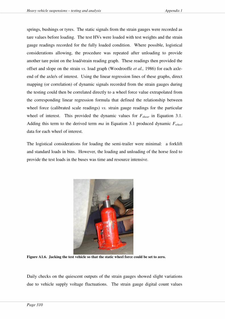
Page 310
Heavy vehicle suspensions – testing and analysis Appendix 1
springs, bushings or tyres. The static signals from the strain gauges were recorded as
tare values before loading. The test HVs were loaded with test weights and the strain
gauge readings recorded for the fully loaded condition. Where possible, logistical
considerations allowing, the procedure was repeated after unloading to provide
another tare point on the load/strain reading graph. These readings then provided the
offset and slope on the strain vs. load graph (Woodrooffe et al., 1986) for each axle-
end of the axle/s of interest. Using the linear regression lines of these graphs, direct
mapping (or correlation) of dynamic signals recorded from the strain gauges during
the testing could then be correlated directly to a wheel force value extrapolated from
the corresponding linear regression formula that defined the relationship between
wheel force (calibrated scale readings) vs. strain gauge readings for the particular
wheel of interest. This provided the dynamic values for Fshear in Equation 3.1.
Adding this term to the derived term ma in Equation 3.1 produced dynamic Fwheel
data for each wheel of interest.
The logistical considerations for loading the semi-trailer were minimal: a forklift
and standard loads in bins. However, the loading and unloading of the horse feed to
provide the test loads in the buses was time and resource intensive.
Figure A1.6. Jacking the test vehicle so that the static wheel force could be set to zero.
Daily checks on the quiescent outputs of the strain gauges showed slight variations
due to vehicle supply voltage fluctuations. The strain gauge digital count values
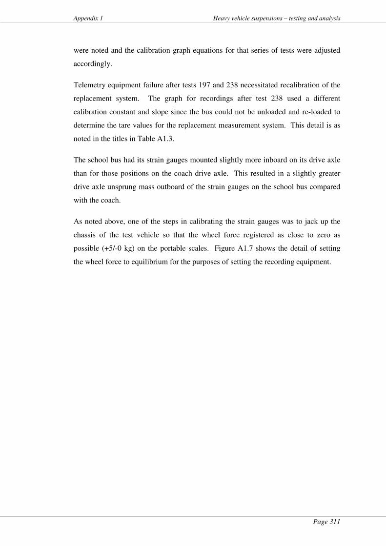
Page 311
Appendix 1 Heavy vehicle suspensions – testing and analysis
were noted and the calibration graph equations for that series of tests were adjusted
accordingly.
Telemetry equipment failure after tests 197 and 238 necessitated recalibration of the
replacement system. The graph for recordings after test 238 used a different
calibration constant and slope since the bus could not be unloaded and re-loaded to
determine the tare values for the replacement measurement system. This detail is as
noted in the titles in Table A1.3.
The school bus had its strain gauges mounted slightly more inboard on its drive axle
than for those positions on the coach drive axle. This resulted in a slightly greater
drive axle unsprung mass outboard of the strain gauges on the school bus compared
with the coach.
As noted above, one of the steps in calibrating the strain gauges was to jack up the
chassis of the test vehicle so that the wheel force registered as close to zero as
possible (+5/-0 kg) on the portable scales. Figure A1.7 shows the detail of setting
the wheel force to equilibrium for the purposes of setting the recording equipment.
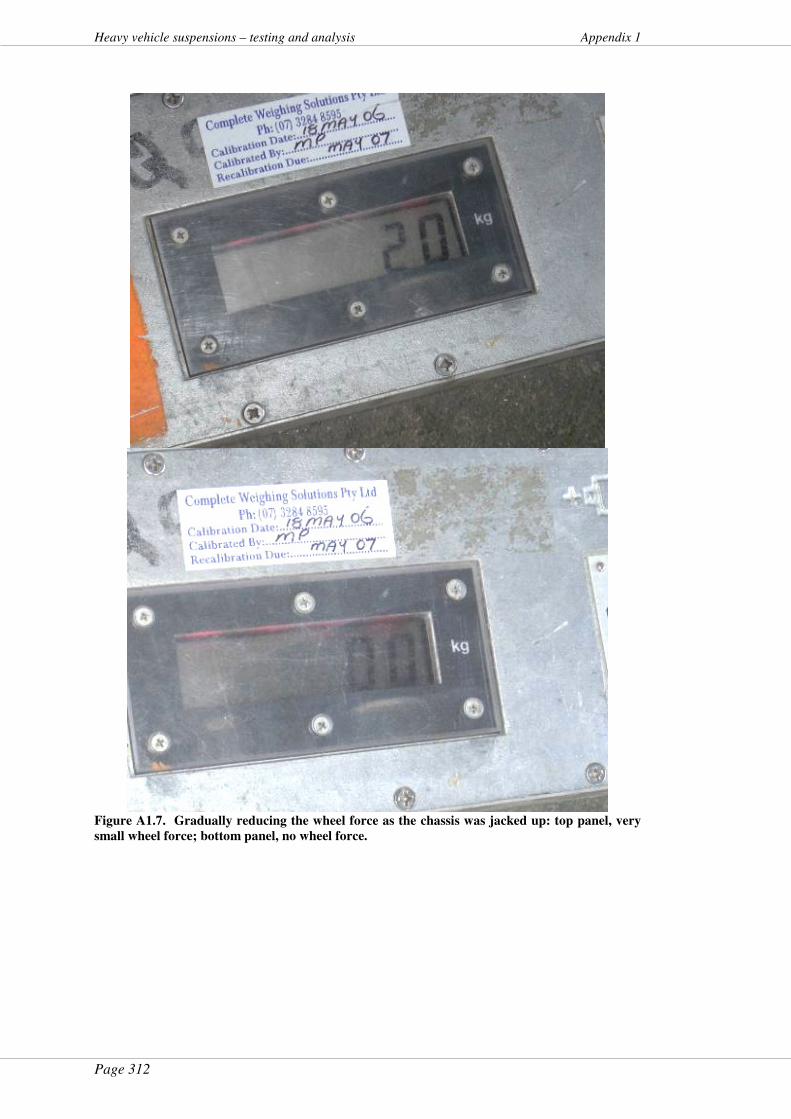
Page 312
Heavy vehicle suspensions – testing and analysis Appendix 1
Figure A1.7. Gradually reducing the wheel force as the chassis was jacked up: top panel, very
small wheel force; bottom panel, no wheel force.
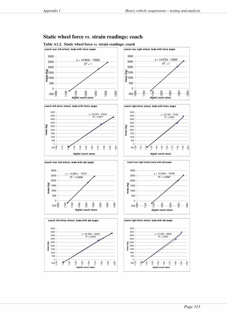
Page 313
Appendix 1 Heavy vehicle suspensions – testing and analysis
Static wheel force vs. strain readings: coach
Table A1.2. Static wheel force vs. strain readings: coach
coach rear left wheel, tests with haire suspn
y = 13.843x - 15682
R2 = 1
-500
0
500
1000
1500
2000
2500
30001050
1100
1150
1200
1250
1300
1350
digital count value
mass (
kg
)
coach rear right wheel, tests with haire suspn
y = 14.672x - 16923
R2 = 1
-500
0
500
1000
1500
2000
2500
3000
105
0
110
0
115
0
120
0
125
0
130
0
135
0
digital count value
ma
ss
(k
g)
coach left drive wheel, tests with haire suspn
y = 56.467x - 63644
R2 = 0.9977
-500
0
500
1000
1500
2000
2500
3000
3500
4000
4500
110
0
111
0
112
0
113
0
114
0
115
0
116
0
117
0
118
0
119
0
120
0
digital count value
mass (
kg
)
coach right drive wheel, tests with haire suspn
y = 62.156x - 70192
R2 = 0.9952
-500
0
500
1000
1500
2000
2500
3000
3500
4000
4500
11
00
11
10
11
20
11
30
11
40
11
50
11
60
11
70
11
80
11
90
12
00
digital count value
ma
ss
(k
g)
coach rear left wheel, tests with std suspn
y = 13.881x - 15721
R2 = 0.9998
-500
0
500
1000
1500
2000
2500
3000
1050
1100
1150
1200
1250
1300
1350
1400
1450
digital count value
mass (
kg
)
coach rear right wheel, tests with std suspn
y = 14.554x - 16795
R2 = 0.9997
-500
0
500
1000
1500
2000
2500
3000
105
0
110
0
115
0
120
0
125
0
130
0
135
0
digital count value
mas
s (
kg
)
coach left drive wheel, tests with std suspn
y = 56.485x - 63663
R2 = 0.9976
-500
0
500
1000
1500
2000
2500
3000
3500
4000
4500
1110
1120
1130
1140
1150
1160
1170
1180
1190
1200
digital count value
ma
ss (
kg
)
coach right drive wheel, tests with std suspn
y = 61.609x - 69582
R2 = 0.9922
-500
0
500
1000
1500
2000
2500
3000
3500
4000
4500
11
10
11
20
11
30
11
40
11
50
11
60
11
70
11
80
11
90
12
00
digital count value
ma
ss
(k
g)
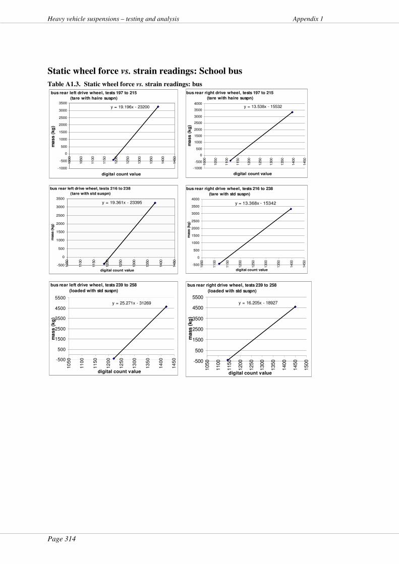
Page 314
Heavy vehicle suspensions – testing and analysis Appendix 1
Static wheel force vs. strain readings: School bus
Table A1.3. Static wheel force vs. strain readings: bus
bus rear left drive wheel, tests 197 to 215
(tare with haire suspn)
y = 19.196x - 23200
-1000
-500
0
500
1000
1500
2000
2500
3000
3500
1000
1050
1100
1150
1200
1250
1300
1350
1400
1450
digital count value
mass (
kg
)
bus rear right drive wheel, tests 197 to 215
(tare with haire suspn)
y = 13.538x - 15532
-1000
-500
0
500
1000
1500
2000
2500
3000
3500
4000
1000
1050
1100
1150
1200
1250
1300
1350
1400
1450
digital count value
mass (
kg
)
bus rear left drive wheel, tests 216 to 238
(tare with std suspn)
y = 19.361x - 23395
-500
0
500
1000
1500
2000
2500
3000
3500
1050
1100
1150
1200
1250
1300
1350
1400
1450
digital count value
mass (
kg
)
bus rear right drive wheel, tests 216 to 238
(tare with std suspn)
y = 13.368x - 15342
-500
0
500
1000
1500
2000
2500
3000
3500
40001050
1100
1150
1200
1250
1300
1350
1400
1450
digital count value
mass (
kg
)
bus rear left drive wheel, tests 239 to 258
(loaded with std suspn)
y = 25.271x - 31269
-500
500
1500
2500
3500
4500
5500
10
50
11
00
11
50
12
00
12
50
13
00
13
50
14
00
14
50
digital count value
ma
ss
(k
g)
bus rear right drive wheel, tests 239 to 258
(loaded with std suspn)
y = 16.205x - 18927
-500
500
1500
2500
3500
4500
5500
1050
1100
1150
1200
1250
1300
1350
1400
1450
1500
digital count value
mass (
kg
)
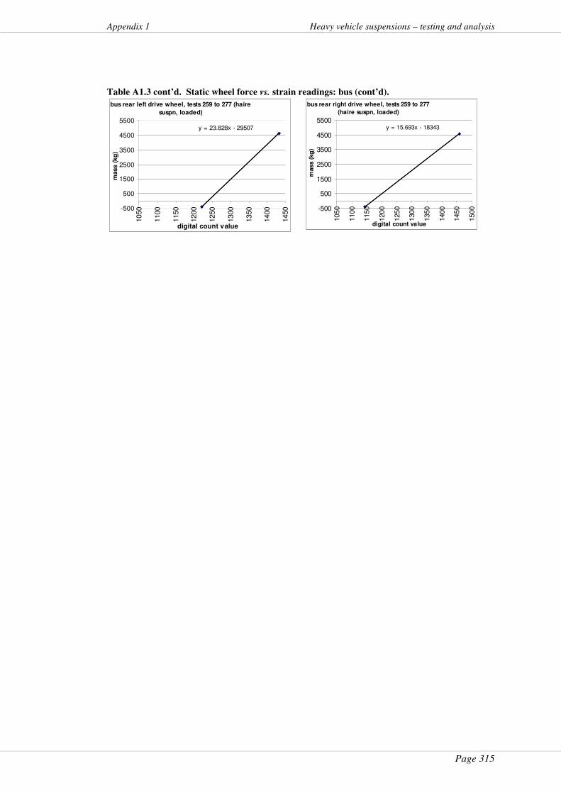
Page 315
Appendix 1 Heavy vehicle suspensions – testing and analysis
Table A1.3 cont’d. Static wheel force vs. strain readings: bus (cont’d).
bus rear left drive wheel, tests 259 to 277 (haire
suspn, loaded)
y = 23.828x - 29507
-500
500
1500
2500
3500
4500
5500
1050
1100
1150
1200
1250
1300
1350
1400
1450
digital count value
mass (
kg
)
bus rear right drive wheel, tests 259 to 277
(haire suspn, loaded)
y = 15.693x - 18343
-500
500
1500
2500
3500
4500
5500
1050
1100
1150
1200
1250
1300
1350
1400
1450
1500
digital count value
mass (
kg
)
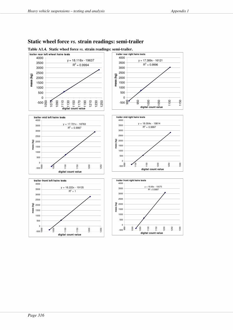
Page 316
Heavy vehicle suspensions – testing and analysis Appendix 1
Static wheel force vs. strain readings: semi-trailer
Table A1.4. Static wheel force vs. strain readings: semi-trailer.
trailer rear left wheel haire tests
y = 18.118x - 19637
R2 = 0.9994
-500
0
500
1000
1500
2000
2500
3000
3500
4000
105
0
107
0
109
0
111
0
113
0
115
0
117
0
119
0
121
0
123
0
125
0
digital count value
mass (
kg
)
trailer rear right haire tests
y = 17.389x - 16121
R2 = 0.9996
-500
0
500
1000
1500
2000
2500
3000
3500
4000
900
950
1000
1050
1100
1150
digital count value
mass (
kg
)
trailer mid left haire tests
y = 17.721x - 18763
R2 = 0.9997
-500
0
500
1000
1500
2000
2500
3000
3500
4000
1000
1050
1100
1150
1200
1250
digital count value
ma
ss (
kg
)
trailer mid right haire tests
y = 18.004x - 19814
R2 = 0.9997
-500
0
500
1000
1500
2000
2500
3000
3500
4000
1050
1100
1150
1200
1250
1300
digital count value
mass (
kg
)
trailer front left haire tests
y = 18.222x - 19135
R2 = 1
-500
0
500
1000
1500
2000
2500
3000
3500
4000
10
00
10
50
11
00
11
50
12
00
12
50
digital count value
mass (
kg
)
trailer front right haire tests
y = 18.66x - 19375
R2 = 0.9997
-500
0
500
1000
1500
2000
2500
3000
3500
4000
950
1000
1050
1100
1150
1200
1250
1300
digital count value
mas
s (
kg
)

Page 317
Appendix 1 Heavy vehicle suspensions – testing and analysis
Table A1.4 cont’d. Static wheel force vs. strain readings: semi-trailer (cont’d).
trailer rear left std testsy = 18.591x - 20159
R2 = 0.9999
-500
0
500
1000
1500
2000
2500
3000
1050
1070
1090
1110
1130
1150
1170
1190
1210
1230
1250
digital count value
mass (
kg
)
trailer rear right std tests
y = 17.413x - 16131
R2 = 0.9991
-500
0
500
1000
1500
2000
2500
3000
3500
900
950
1000
1050
1100
1150
digital count value
mass (
kg
)
trailer mid left std testsy = 17.953x - 18977
R2 = 0.9986
-500
0
500
1000
1500
2000
2500
3000
100
0
105
0
110
0
115
0
120
0
125
0
digital count value
mass (
kg
)
trailer mid right std testsy = 18.061x - 19894
R2 = 0.9989
-500
0
500
1000
1500
2000
2500
3000
10
50
11
00
11
50
12
00
12
50
13
00
digital count value
mas
s (
kg
)
trailer front left std testsy = 18.007x - 18890
R2 = 0.9999
-500
0
500
1000
1500
2000
2500
3000
100
0
105
0
110
0
115
0
120
0
125
0
digital count value
mass (
kg
)
trailer front right std tests
y = 18.573x - 19304
R2 = 1
-500
0
500
1000
1500
2000
2500
3000
3500
950
10
00
10
50
11
00
11
50
12
00
12
50
digital count value
mas
s (
kg
)
Page 318
Heavy vehicle suspensions – testing and analysis Appendix 2
Appendix 2 – Error analysis for the three test HVs
The details following have been outlined elsewhere (Davis & Bunker, 2008d; Davis
& Bunker, 2009e). The dynamic and inertial forces at the wheels of a HV are in a
constant state of flux during travel. An overall conclusive error value which holds
for all conditions is therefore virtually impossible to derive (Cole, 1990). The work
of Cole (1990) and, slightly earlier, Mitchell and Gyenes (1989), examined dynamic
suspension measures. That work was, in part, trying to allocate indicators to
different types of HV suspensions.
The test programme for the three HVs tested for this thesis recorded the dynamic
shear forces on the axles at the strain gauges and any dynamic forces from the axles
outboard of strain gauges due to the inertial mass of the wheels and other outboard
components. This was achieved with axle strain gauges and accelerometers. The
readings from these were used to derive both static and dynamic wheel forces. This
method used modern instrumentation to reduce error compared with previous
methods. Cole (1990) proposed an error of approximately 7 percent due to that work
not measuring, nor recording, the unsprung mass outboard of the axle strain gauges.
This meant that forces from the dynamic inertia outboard of the strain gauges were
not derived. Overall dynamic wheel forces were, at best, estimated as a contribution
to the totality of dynamic wheel forces (Cole, 1990).
The overall errors in wheel force measurements from the programme for this thesis
were due to the errors in the accelerometer, telemetry system, rd ≠ (Figure 3.15),
and strain gauge readings. Overall error in the telemetry system used for these tests
has been documented previously at ±1.0 percent (Davis, 2006b). This has been
verified by the OBM test programme (Karl et al., 2009b). The individual error of
each strain gauge reading by the telemetry system used for these tests can be seen in
Table A1.2 to Table A1. The regression values varied from 99.22 percent, or an
error of less than one percent at worst for one strain gauge on the coach, to 100
percent (best) for the semi-trailer. These figures indicate that the errors in strain
gauge readings were, even at the worst, very small.
Nonetheless, a cross check for overall error was undertaken, and an indicative error
value ascribed from the results for the bus, as follows:

Page 319
Appendix 2 Heavy vehicle suspensions – testing and analysis
� noting that the telemetry system sampled at 1 kHz for 10 s per run;
1 x 10⁴ instantaneous values from each strain gauge and
accelerometer were recorded per test run;
� the bus LSC was derived (Figure A2.1) by averaging those 1 x 10⁴
values across all transducers (by definition, since LSC requires an
averaging process for its derivation);
� LSC uses an average of instantaneous wheel force for each run and
divides it by the mean (or static) wheel force of the group during the
test; but
� the bus had only 2 wheels under test, therefore:
� the bus LSC for each test speed should therefore have been 1.0.
Any deviation from 1.0 for the bus LSC was therefore due to a combined
measurement error at the strain gauges, the telemetry system and the accelerometers.
The worst-case LSC (i.e. largest error) at each test speed for the bus was plotted in
Figure A2.1. This indicated that the measurement error ranged from -2.2 percent to
+3.2 percent. Hence an error range of +/- 3 percent seems a reasonable conclusion.
Further, for any instantaneous metrics such as the dynamic load sharing coefficient
(DLSC), the averaging process was not used. Therefore, any error would be per
instantaneous reading. Instantaneous reading error vs. the compounded error for
averaged metrics would be reduced proportionally to the number of samples. With 1
x 104 samples, this made any error in instantaneous metrics very small.
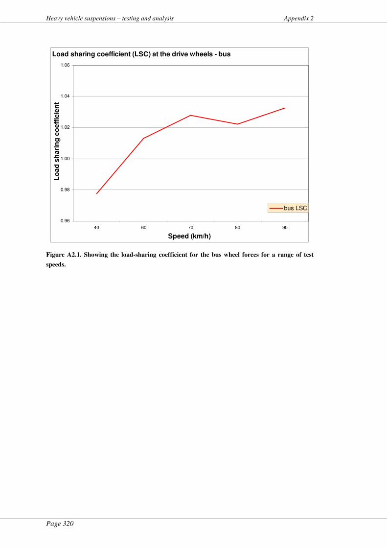
Page 320
Heavy vehicle suspensions – testing and analysis Appendix 2
Load sharing coefficient (LSC) at the drive wheels - bus
0.96
0.98
1.00
1.02
1.04
1.06
40 60 70 80 90
Speed (km/h)
Lo
ad
sh
ari
ng
co
eff
icie
nt
bus LSC
Figure A2.1. Showing the load-sharing coefficient for the bus wheel forces for a range of test
speeds.
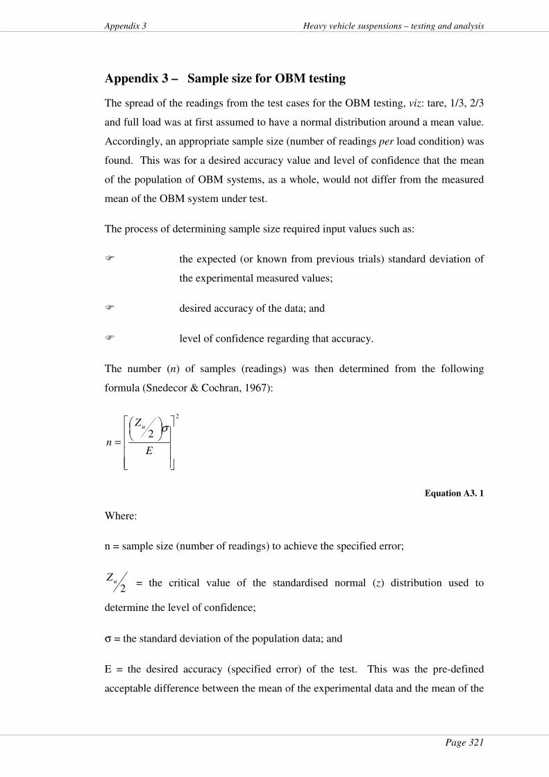
Page 321
Appendix 3 Heavy vehicle suspensions – testing and analysis
Appendix 3 – Sample size for OBM testing
The spread of the readings from the test cases for the OBM testing, viz: tare, 1/3, 2/3
and full load was at first assumed to have a normal distribution around a mean value.
Accordingly, an appropriate sample size (number of readings per load condition) was
found. This was for a desired accuracy value and level of confidence that the mean
of the population of OBM systems, as a whole, would not differ from the measured
mean of the OBM system under test.
The process of determining sample size required input values such as:
� the expected (or known from previous trials) standard deviation of
the experimental measured values;
� desired accuracy of the data; and
� level of confidence regarding that accuracy.
The number (n) of samples (readings) was then determined from the following
formula (Snedecor & Cochran, 1967):
2
2
=E
Z
n
u σ
Equation A3. 1
Where:
n = sample size (number of readings) to achieve the specified error;
2uZ
= the critical value of the standardised normal (z) distribution used to
determine the level of confidence;
σ = the standard deviation of the population data; and
E = the desired accuracy (specified error) of the test. This was the pre-defined
acceptable difference between the mean of the experimental data and the mean of the

Page 322
Heavy vehicle suspensions – testing and analysis Appendix 3
total population6.
The value of 2
uZ was determined from the choice of the level of significance
known as α which was, in turn, used to derive the level of confidence. The level of
confidence is usually designated as a percentage that can be visualised as being
bounded by the critical values of +/-2
uZ under the normal population distribution
curve (Davis et al., 2008a, 2008b) and related to half of the level of significance
(α/2) therein.
The level of confidence is a value (or percentage) of certainty that the mean of the
sample data will be within the specified error of the mean of the entire population.
The level of confidence is designated:
1 - α as a value; or
(1 - α) x 100 as a percentage.
For instance, a value of α = 0.1 provides a level of confidence of 0.90 or 90 percent
that the mean value in the sample readings will be equal to or smaller than the
desired error of the population mean (Snedecor & Cochran, 1967).
The OBM pilot test plan used an initial value for standard deviation (σ) of 350 kg
from earlier work (Davis, 2006b). Early in the pilot testing a maximum value for σ
for OBM readings of 130 kg for loads approximating 22 t was observed. These
results, and choosing a maximum value of E as 140 kg for loads of 22 t
(approximately), led to the following calculations to choose the number of readings:
to find the number of readings required to determine the mean accuracy of OBM
systems for:
� a level of confidence of 95 percent; and
� a standard deviation σ of 130 kg7; with
6 In this case, the total population would be the total population of OBM systems.
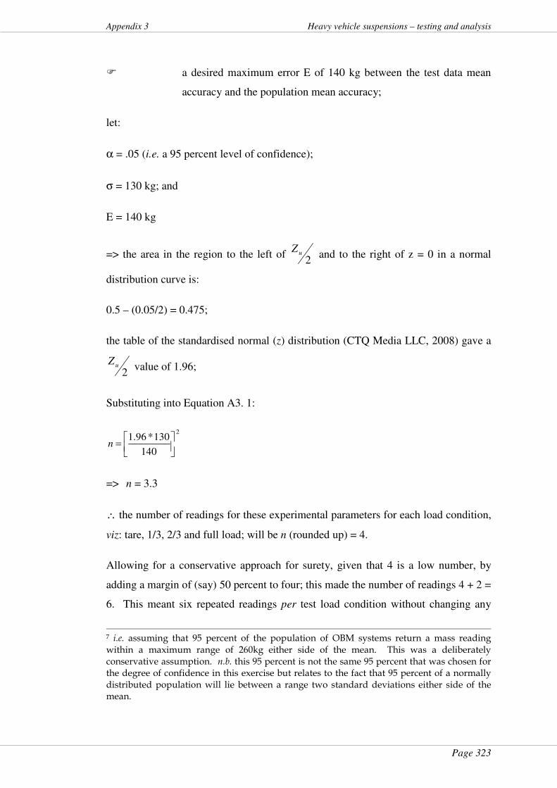
Page 323
Appendix 3 Heavy vehicle suspensions – testing and analysis
� a desired maximum error E of 140 kg between the test data mean
accuracy and the population mean accuracy;
let:
α = .05 (i.e. a 95 percent level of confidence);
σ = 130 kg; and
E = 140 kg
=> the area in the region to the left of 2
uZ and to the right of z = 0 in a normal
distribution curve is:
0.5 – (0.05/2) = 0.475;
the table of the standardised normal (z) distribution (CTQ Media LLC, 2008) gave a
2uZ
value of 1.96;
Substituting into Equation A3. 1:
2
140
130*96.1
=n
=> n = 3.3
∴ the number of readings for these experimental parameters for each load condition,
viz: tare, 1/3, 2/3 and full load; will be n (rounded up) = 4.
Allowing for a conservative approach for surety, given that 4 is a low number, by
adding a margin of (say) 50 percent to four; this made the number of readings 4 + 2 =
6. This meant six repeated readings per test load condition without changing any
7 i.e. assuming that 95 percent of the population of OBM systems return a mass reading within a maximum range of 260kg either side of the mean. This was a deliberately conservative assumption. n.b. this 95 percent is not the same 95 percent that was chosen for the degree of confidence in this exercise but relates to the fact that 95 percent of a normally distributed population will lie between a range two standard deviations either side of the mean.

Page 324
Heavy vehicle suspensions – testing and analysis Appendix 3
other variables.
The choice of 6 readings was validated in the middle and latter stages of the pilot
testing where the values of σ (standard deviation of the test and reference system
population data) were about or below 140 kg after anomalous data were removed
(Germanchev & Eady, 2008).
The conservative approach of six readings increased the level of confidence and
reduced the value of E to approximately 100 kg when the maximum value for σ
dropped below 90 kg.
Page 325
Appendix 4 Heavy vehicle suspensions – testing and analysis
Appendix 4 – Copyright release
The document (Australia Department of Transport, 1979) from which the diagrams
in Figure 1.1 and Figure 1.2 have been taken is not copyright.
The diagram in Figure 1.3 was originally developed by John Woodrooffe
(Woodrooffe, 1997) and reproduced in the DIVINE report (OECD, 1998). Kind
permission has been granted by the original author to reproduce the diagram. This
permission is shown below (Figure A4.1).
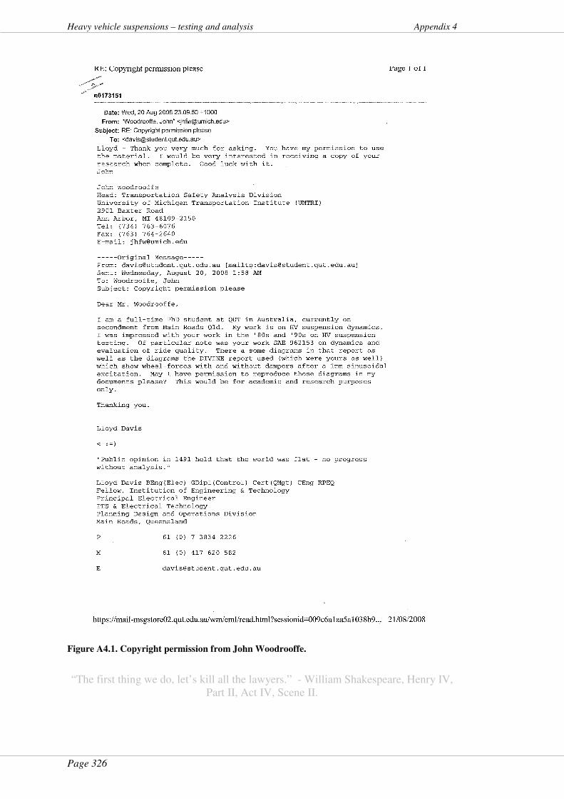
Page 326
Heavy vehicle suspensions – testing and analysis Appendix 4
Figure A4.1. Copyright permission from John Woodrooffe.
“The first thing we do, let’s kill all the lawyers.” - William Shakespeare, Henry IV,
Part II, Act IV, Scene II.
Page 327
Appendix 5 Heavy vehicle suspensions – testing and analysis
Appendix 5 – Publications
QUT & MR/DTMR publications
Davis, L. and Bunker, J. (2010). Determining heavy vehicle suspension health from vibratory wheel loads. International Heavy Vehicle Transport Technology Symposium, 11th, 2010, Melbourne, Victoria, Australia.
Davis, L. and Bunker, J. (2010). Dynamic Load Sharing for Heavy Vehicles - a New Metric. Road and Transport Research, Vol. 18 No. 4 (invited paper). ARRB Group,
Vermont South, Victoria, Australia.
Davis, L. and Bunker, J. (2009). Determining heavy vehicle suspension health from vibratory wheel loads. Smart Systems Student Conference, 3rd, Oct 2009, Queensland University of Technology, Brisbane, Queensland, Australia.
Davis, L. and Bunker, J. (2009). Altering Heavy Vehicle air suspension dynamic forces by modifying air lines. International Journal of Heavy Vehicle Systems. Inderscience Publications, Geneve, Switzerland. (paper accepted but not yet published).
Davis, L. and Bunker, J. (2009). Mum, why are the potholes 8 feet apart? Repetitive wheel loads from heavy vehicles in the spatial domain. Paper presented at the Main Roads Technology Forum, 15th, 2009, Brisbane, Queensland, Australia.
Davis, L. and Bunker, J. (2009). Development of a software model of a heavy vehicle suspension for research. Built Environment and Engineering Postgraduate Student Conference, 26th March 2009, Queensland University of Technology, Brisbane, Queensland, Australia.
Davis, L. and Bunker, J. (2009). Heavy vehicle suspension testing and analysis: dynamic load sharing. Report. Department of Main Roads and Queensland University of Technology, Brisbane, Queensland, Australia.
Davis, L. and Bunker, J. (2009). Heavy vehicle suspensions: testing and analysis. Phase 3 - Eigenfrequency peak loads: measuring suspension health from wheel loads. Preliminary test report. Department of Main Roads and Queensland University of Technology, Brisbane, Queensland, Australia.
Davis, L. and Bunker, J. (2009). Load-sharing in heavy vehicle suspensions: new metrics for old. Built Environment and Engineering Postgraduate Student Conference, 26th March 2009, Queensland University of Technology, Brisbane, Queensland, Australia. Also submitted to Road & Transport Research.
Davis, L. and Bunker, J. (2009). Suspension testing of 3 heavy vehicles - dynamic wheel force analysis - Report. State of Queensland (Department of Main Roads) & Queensland University of Technology, Brisbane, Queensland, Australia.
Davis, L. and Bunker, J. (2008). Characterising heavy vehicle suspensions – impulse testing results and analysis. Department of Main Roads and Queensland University of Technology, Brisbane, Queensland, Australia.
Page 328
Heavy vehicle suspensions – testing and analysis Appendix 5
Davis, L. and Bunker, J. (2008). Heavy Vehicle Suspensions - Testing and Analysis: Phase 3 - Eigenfrequency peak loads. Test Plan. Department of Main Roads and Queensland University of Technology, Brisbane, Queensland, Australia.
Davis, L. and Bunker, J. M. (2008). In-service testing of heavy vehicle suspensions: background report for the NTC project. Department of Main Roads and Queensland University of Technology, Brisbane, Queensland, Australia.
Davis, L. and Bunker, J. (2008). In-service suspension testing of heavy vehicles – update on recent test programme and proof-of-concept. Built Environment and Engineering Postgraduate Student Conference, 10 September 2008, Queensland University of Technology, Brisbane, Queensland, Australia.
Davis, L. and Bunker, J. M. (2008). Larger air lines in HV suspensions – differences in wheel and air spring forces. Australasian Transport Research Forum, 31st, 2008, Gold Coast, Queensland, Australia.
Davis, L. and Bunker, J. (2008). Suspension testing of 3 heavy vehicles – methodology and preliminary frequency analysis. Report. State of Queensland (Department of Main Roads) and Queensland University of Technology, Brisbane, Queensland, Australia.
Davis, L. and Bunker, J. (2007). Heavy Vehicle Suspensions – Testing and Analysis. A literature review. Department of Main Roads and Queensland University of Technology, Brisbane, Queensland, Australia.
QUT, MR/DTMR and TCA publications
Karl, C., Cai, D., Davis, L. and Bunker, J. (2010). Tamper Evidence for Heavy Vehicle On-Board Mass Systems. ARRB Conference 24th, 2010, Melbourne, Victoria, Australia. (paper accepted but not yet published).
Davis, L., Bunker, J. and Karl, C. (2009). Technical feasibility assessment of on-board mass-monitoring (OBM) devices: a) accuracy and robustness b) ancillary systems analysis: frequency analysis report. Department of Main Roads, Queensland University of Technology, Brisbane, Queensland, and Transport Certification Australia, Melbourne; Australia.
Davis, L., Bunker, J. and Karl, C. (2008). Technical feasibility assessment of on-board mass monitoring (OBM) devices: a) Accuracy and robustness b) Ancillary systems analysis. Full-scale testing plan. Department of Main Roads, Queensland University of Technology, Brisbane, Queensland, and Transport Certification Australia, Melbourne; Australia.
Davis, L., Bunker, J. and Karl, C. (2008). Technical feasibility assessment of on-board mass monitoring (OBM) devices: a) Accuracy and robustness b) Ancillary systems analysis. Pilot test plan. Department of Main Roads, Queensland University of Technology, Brisbane, Queensland, and Transport Certification Australia, Melbourne, Australia.
Page 329
Appendix 5 Heavy vehicle suspensions – testing and analysis
QUT, MR/DTMR, ARRB and TCA publications
Karl, C., Cai, D., Davis, L., Bunker, J., Germanchev, A., Eady, P., and Blanksby, C. (2010). On-Board Mass Monitoring of Heavy Vehicles - Results of Testing Program. Journal of Road and Transport Research. ARRB Group, Melbourne, Victoria, Australia. (paper accepted but not yet published).
Davis, L., Karl, C., Cai, D., Blanksby, C., Germanchev, A., and Eady, P. (2010). Static accuracy and precision of heavy vehicle on-board mass systems testing results. International Heavy Vehicle Transport Technology Symposium, 11th, 2010, Melbourne, Victoria, Australia.
Davis, L., Karl, C., Cai, D., Blanksby, C., Germanchev, A. and Eady, P. (2010). Dynamic analysis of on-board mass data to determine tampering in heavy vehicle on-board mass systems. International Heavy Vehicle Transport Technology Symposium, 11th, 2010, Melbourne, Victoria, Australia.
TCA Publications
Karl, C., Cai, D., Koniditsiotis, C. and Davis, L. (2009). A regulatory on-board mass monitoring application for heavy vehicles in Australia. World Congress on Intelligent Transport Systems, 16th, 2009, Stockholm, Sweden.
Karl, C., Davis, L., Cai, D., Blanksby, C., Germanchev, A., Eady, P. and Harcourt, R. (2009). On-board mass monitoring test report (final). Transport Certification Australia, Melbourne, Australia.
Cai, D., Davis, L. and Karl, C. (2008). The development of an evidentiary on-board mass monitoring application for heavy vehicles. World Congress on Intelligent Transport Systems, 15th, 2008, New York, NY, USA.
MR Publications
Davis, L., (2007). Further developments in dynamic testing of heavy vehicle suspensions. Australasian Transport Research Forum, 30th, 2007, Melbourne, Victoria, Australia.
Davis, L., Kel, S. and Sack, R. (2007). Further development of in-service suspension testing for heavy vehicles. Australasian Transport Research Forum, 30th, 2007, Melbourne, Australia. John H Taplin Prize – best scientific paper 2007.
Davis, L., & Kel, S. (2007). Heavy vehicle suspension testing: parametric changes from larger longitudinal air lines; Innovative systems for heavy vehicle suspension testing. Paper presented at the Main Roads Technology Forum, 13th, 2007, Brisbane, Queensland, Australia.
Heavy vehicle suspensions – testing and analysis References
Page 330
References
Australian vehicle standards rules 1999: statutory rules 1999; no. 1, Road Transport Reform (Vehicles and Traffic) Act 1993, (1999).
Australia Department of Transport. (1979). Advisory committee on vehicle performance. A
guide to heavy vehicle suspension systems and acceptable axle groups. Canberra, ACT, Australia: Australian Government publishing service.
Australia Department of Transport and Regional Services. (2004a). Certification of road-
friendly suspension systems; Road-friendly suspension certification requirements. Canberra, ACT, Australia: Australia. Department of Transport and Regional Services (DoTaRS).
Australia Department of Transport and Regional Services. (2004b). Certified road-friendly
suspensions. Retrieved 3 August 2007, from http://www.infrastructure.gov.au/roads/vehicle_regulation/suspension.aspx.
Australia Department of Transport and Regional Services. (2004c). Vehicle Standards
Bulletin No.11. Retrieved 6 Sept 2007, from http://www.infrastructure.gov.au/roads/vehicle_regulation/bulletin/pdf/vsb_11.pdf.
Australia Department of Transport and Regional Services. (2005a). Bilateral agreement
between the Commonwealth of Australia and the State of New South Wales 2004 - 2009. Retrieved 7 September 2007, 2007, from http://www.auslink.gov.au/publications/policies/pdf/NSW_Bilateral.pdf.
Australia Department of Transport and Regional Services. (2005b). Bilateral agreement
between the Commonwealth of Australia and the State of Queensland 2004-05 – 2008-09. Retrieved 7 September 2007, 2007, from http://www.auslink.gov.au/publications/policies/pdf/Qld_bilateral.pdf.
Australian Road Transport Suppliers Association. (2001). Air suspension code – Guidelines
for maintaining and servicing air suspensions for heavy vehicles. South Melbourne, Victoria, Australia: Australian Road Transport Suppliers Association (ARTSA).
Austroads. (1992). Pavement design: A guide to the structural design of road pavements. Sydney, NSW, Australia: Austroads.
Bisitecniks. (2007). Road friendly suspension test results. In L. Davis (Ed.) York 9000HL axle test report. Wendouree, Victoria, Australia: Colrain.
Blanksby, C. (2007). Review of 'Testing of heavy vehicle suspensions - Phase 2 Interim
Report'. Melbourne, Australia: ARRB Group.
Blanksby, C., George, R., Germanchev, A., Patrick, S. & Marsh, F. (2006). In-service survey
of heavy vehicle suspensions. ARRB contract report VC71235-01-01 08/2006. Sydney, Australia: ARRB Group, Roads and Traffic Authority of NSW.
Blanksby, C., George, R., Peters, B., Ritzinger, A. & Bruzsa, L. (2008). Measuring dynamic wheel loads on tri and quad axle groups. International Conference on Heavy Vehicles, Paris, France: London, UK: ISTE & Wiley.
Page 331
References Heavy vehicle suspensions – testing and analysis
Blanksby, C., Germanchev, A., Ritzinger, A., Elischer, M. & George, R. (2009). Measuring
the dynamic wheel loads of heavy vehicles. Sydney, NSW, Australia: Austroads.
Brigham, E. O. (1988). The fast Fourier transform and its applications. Englewood Cliffs, New Jersey, USA: Prentice-Hall.
Cebon, D. (1987). Assessment of the dynamic wheel forces generated by heavy road vehicles. Symposium on Heavy Vehicle Suspension Characteristics, Canberra, Australia: Vermont South, Victoria, Australia: Australian Road Research Board (ARRB).
Cebon, D. (1999). Handbook of vehicle-road interaction. Lisse, South Holland, Netherlands: Swets & Zeitlinger.
Chatti, K. & Lee, D. (2002). Development of new profile-based truck dynamic load index. Transportation Research Record, 1806, 149 - 159.
Chesmond, C. J. (1982). Control system technology (2nd ed.). Caulfield, Victoria, Australia: Edward Arnold.
Clarke, H. & Prentice, D. (2009). A conceptual framework for the reform of taxes related to
roads and transport. Melbourne, Victoria, Australia: La Trobe University.
Cole, D. J. (1990). Measurement and analysis of dynamic tyre forces generated by lorries. University of Cambridge, Cambridge, United Kingdom.
Cole, D. J. & Cebon, D. (1989). A capacitive strip sensor for measuring dynamic tyre forces. In Institution of Electrical Engineers (Ed.), International conference of road traffic
monitoring 2nd, London, United Kingdom: London, United Kingdom: Institution of Electrical Engineers.
Cole, D. J. & Cebon, D. (1991). Assessing the road-damaging potential of heavy vehicles. Journal of Automobile Engineering Proc. I.Mech.E, 205 (D4), 223 - 232.
Cole, D. J. & Cebon, D. (1992). Spatial repeatability of dynamic tyre forces generated by heavy vehicles. Journal of Automobile Engineering Proc. I.Mech.E, 206 (D3), 185 - 197.
Cole, D. J. & Cebon, D. (1994). Predicting vertical dynamic tire forces of heavy trucks. Vehicle-Road Interaction II Conference, Santa Barbara, California, USA: Philadelphia, Pennsylvania, USA: American Society for Testing and Materials.
Cole, D. J. & Cebon, D. (2007). Truck tyres, suspension design to minimise road damage. Retrieved 26 October 2007, from http://www-mech.eng.cam.ac.uk/trg/publications/downloads/veh_road/veh_road17.pdf.
Cole, D. J., Collop, A. C., Potter, T. E. C. & Cebon, D. (1992). Use of a force measuring mat to compare the road damaging potential of heavy vehicles. In D. Cebon & C. G. B. Mitchell (Eds.), Heavy vehicles and roads: technology, safety and policy (pp. 266 - 271). London, United Kingdom: Thomas Telford.
Cole, D. J., Collop, A. C., Potter, T. E. C. & Cebon, D. (1996). Spatial repeatability of measured dynamic tyre forces. Proceedings of the Institution of Mechanical Engineers,
Part D, Journal of Automobile Engineering, 210 (D3), 185 - 197.
Collop, A. C. & Cebon, D. (2002). The benefits of road-friendly suspensions. International
Conference on Asphalt Pavements, 9th, Copenhagen, Denmark: Copenhagen, Denmark: The Danish Road Directorate, Ministry of Transport.
Heavy vehicle suspensions – testing and analysis References
Page 332
Collop, A. C., Cebon, D. & Cole, D. J. (1996). Effects of spatial repeatability on long-term flexible pavement performance. Proceedings of the Institution of Mechanical Engineers,
Part C: Journal of Mechanical Engineering Science, 210 (C2), 97 - 111.
Collop, A. C., Potter, T. E. C., Cebon, D. & Cole, D. J. (1994). Investigation of spatial repeatability using a tyre force measuring mat. Transportation Research Record, 1448, 1 - 7.
Colrain. (2007). Bisitecniks road friendly suspension test results York 9000HL axle test
report. Wendouree, Victoria, Australia: Colrain
Considine, D. M. (Ed.). (1985). Process instruments and controls handbook. New York, New York, USA: McGraw-Hill.
Continental tyres. (2005). Technical data book. Retrieved 16 Nov 2005, from http://www.contionline.com/generator/www/uk/en/continental/transport/themes/technical_information/literature/download/technic_pdf_en.pdf.
Costanzi, C. & Cebon, D. (2007). An investigation of the effects of lorry suspension performance on road maintenance costs. Journal of Mechanical Engineering Science,
221, 1265 - 1277.
Costanzi, M. & Cebon, D. (2005). Simulation of damage evolution in a spray sealed road.
Technical report CUED/C-MECH/TR.90. Sydney: Cambridge University Engineering Department, Roads and Traffic Authority, NSW, Australia.
Costanzi, M. & Cebon, D. (2006). Simulation of damage evolution in a spray sealed road. International Symposium on Heavy Vehicle Weights and Dimensions, 9th, State College, Pennsylvania, USA: Pennsylvania, USA: Pennsylvania State University.
CTQ Media LLC. (2008). Table of the Standard Normal (z) Distribution. Retrieved 14 February 2008, from http://www.isixsigma.com/library/content/zdistribution.asp.
Davis, L. (2006a). Dynamic load sharing on air-sprung heavy vehicles: can suspensions be made friendlier by fitting larger air lines? Australasian Transport Research Forum
(ATRF), 29th, Gold Coast, Queensland, Australia: ATRF. www.patrec.org/atrf/index.php.
Davis, L. (2006b). Heavy vehicle suspension testing: on-board mass measurement system
accuracy & tamper-vulnerability. Brisbane, Queensland, Australia: Queensland Department of Main Roads.
Davis, L. (2007). Further developments in dynamic testing of heavy vehicle suspensions. Australasian Transport Research Forum (ATRF), 30th, Melbourne, Victoria, Australia: ATRF. www.patrec.org/atrf/index.php.
Davis, L. (2008). Technical Feasibility Assessment of On-Board Mass-Monitoring (OBM)
Devices: a) Accuracy and robustness b) Ancillary systems analysis. Report on trip to
investigate international approach to OBM measurement for HVs. Brisbane, Queensland; Melbourne, Victoria: Queensland Department of Main Roads; Transport Certification Australia.
Davis, L. & Bunker, D. J. (2009a). Mum, why are the potholes 8 feet apart? Repetitive wheel loads from heavy vehicles in the spatial domain. Main Roads Technology Forum,
15th, 2009, Brisbane, Queensland, Australia: Brisbane, Queensland, Australia: Department of Transport and Main Roads.
Page 333
References Heavy vehicle suspensions – testing and analysis
Davis, L. & Bunker, J. (2007). Heavy Vehicle Suspensions – Testing and Analysis. A
literature review. Brisbane, Queensland, Australia: Queensland Department of Main Roads; Queensland University of Technology.
Davis, L. & Bunker, J. (2008a). Characterising heavy vehicle suspensions – impulse testing
results and analysis – Report. Brisbane, Queensland, Australia: Queensland University of Technology & Queensland Main Roads.
Davis, L. & Bunker, J. (2008b). Heavy vehicle suspensions - testing and analysis: Phase 3 -
Eigenfrequency peak loads. Test plan. Brisbane, Queensland, Australia: Queensland University of Technology.
Davis, L. & Bunker, J. (2008c). In-service suspension testing of heavy vehicles – update on recent test programme and proof-of-concept. In S. Lawry & C. Wrigley (Eds.), Design
Theme Postgraduate Student Conference, Brisbane, Queensland, Australia: Brisbane, Queensland, Australia: Queensland University of Technology.
Davis, L. & Bunker, J. (2008d). Larger air lines in heavy vehicle suspensions – differences in wheel and air spring forces. Australasian Transport Research Forum (ATRF), 31st, Gold Coast, Queensland, Australia: ATRF. www.patrec.org/atrf/index.php.
Davis, L. & Bunker, J. (2008e). Suspension testing of 3 heavy vehicles – methodology and
preliminary frequency analysis. Brisbane, Queensland, Australia: Queensland Department of Main Roads; Queensland University of Technology.
Davis, L. & Bunker, J. (2009b). Heavy vehicle suspension testing and analysis: dynamic
load sharing. Report. Brisbane, Queensland, Australia: Department of Main Roads and Queensland University of Technology.
Davis, L. & Bunker, J. (2009c). Heavy vehicle suspensions: testing and analysis. Phase 3 -
Eigenfrequency peak loads: measuring suspension health from wheel loads. Preliminary
test report. Brisbane, Queensland, Australia: Queensland University of Technology.
Davis, L. & Bunker, J. (2009d). Load sharing in heavy vehicle suspensions: new metrics for old. Built Environment and Engineering Postgraduate Student Conference, Brisbane, Queensland, Australia: Brisbane, Queensland, Australia: Queensland University of Technology.
Davis, L. & Bunker, J. (2009e). Suspension testing of 3 heavy vehicles – dynamic wheel
force analysis. Brisbane, Queensland, Australia: Department of Main Roads & Queensland University of Technology.
Davis, L., Bunker, J. & Karl, C. (2008a). Technical Feasibility Assessment of On-Board
Mass-Monitoring (OBM) Devices: a) Accuracy and robustness b) Ancillary systems
analysis. Full-scale test plan. Brisbane, Queensland, & Melbourne, Victoria; Australia: Queensland Department of Main Roads; Queensland University of Technology; Transport Certification Australia.
Davis, L., Bunker, J. & Karl, C. (2008b). Technical Feasibility Assessment of On-Board
Mass-Monitoring (OBM) Devices: a) Accuracy and robustness b) Ancillary systems
analysis. Pilot test plan. Brisbane, Queensland, & Melbourne, Victoria; Australia: Queensland Department of Main Roads; Queensland University of Technology; Transport Certification Australia.
Heavy vehicle suspensions – testing and analysis References
Page 334
Davis, L., Bunker, J. & Karl, C. (2009). Technical feasibility assessment of on-board mass-
monitoring (OBM) devices: a) accuracy and robustness b) ancillary systems analysis:
frequency analysis report. Brisbane, Queensland, & Melbourne, Victoria; Australia: Queensland Department of Main Roads; Queensland University of Technology; Transport Certification Australia.
Davis, L. & Kel, S. (2007). Heavy vehicle suspension testing: parametric changes from larger longitudinal air lines; Innovative systems for heavy vehicle suspension testing. Main Roads Technology Forum, 13th, Brisbane, Queensland, Australia: Brisbane, Queensland, Australia: Department of Main Roads. Engineering and Technology Group.
Davis, L., Kel, S. & Sack, R. (2007). Further development of in-service suspension testing for heavy vehicles. Australasian Transport Research Forum (ATRF), 30th, Melbourne, Victoria, Australia: ATRF. www.patrec.org/atrf/index.php.
Davis, L. & Sack, R. (2004). Analysis of heavy vehicle suspension dynamics using an on-board mass measurement system. Australasian Transport Research Forum (ATRF), 27th, Adelaide, South Australia, Australia: ATRF. www.patrec.org/atrf/index.php.
Davis, L. & Sack, R. (2005). Background data recorded during preparation of paper: 'Dynamic load sharing on air-sprung heavy vehicles: can suspensions be made friendlier by fitting larger air lines?' - unpublished. Queensland Department of Main Roads.
Davis, L. & Sack, R. (2006). Determining heavy vehicle suspension dynamics using an on-board mass measurement system. ARRB Conference, 22nd, Canberra, ACT, Australia: Vermont South, Victoria, Australia: ARRB Group Ltd.
de Pont, J. J. (1992). Using servo-hydraulics to assess heavy vehicle suspensions for road wear. In D. Cebon & C. G. B. Mitchell (Eds.), Heavy vehicles and roads: technology,
safety and policy (pp. 252 - 259). London: Thomas Telford.
de Pont, J. J. (1997). Assessing heavy vehicle suspensions for road wear. Research report
no. 95. Wellington, New Zealand: Transfund New Zealand.
de Pont, J. J. (1999). Suspensions or whole vehicles? Rating road-friendliness. International
Journal of Vehicle Design, 6, 75 - 98.
de Pont, J. J. (2004). Modelling the dynamic wheel forces of the heavy vehicle fleet. International Symposium on Heavy Vehicle Weights and Dimensions, 8th, Muldersdrift, South Africa: Johannesburg, South Africa: Document Transformation Technologies.
de Pont, J. J. & Pidwerbesky, B. (1994). Vehicle dynamics and pavement performance models. Australian Road Research Board Ltd (ARRB) Conference, 17th, Gold Coast, Queensland, Australia: Vermont South, Victoria, Australia: Australian Road Research Board Ltd (ARRB).
de Pont, J. J. & Steven, B. (1999). Suspension dynamics and pavement wear. Conference on
Vehicle-Infrastructure Interaction VI, Zakopane, Poland: Warsaw, Poland: Institute of Fundamental Technological Research.
Doebelin, E. O. (1980). System modelling and response - theoretical and experimental
approaches. New York, New York, USA: Wiley.
Dubes, R. C. (1968). The theory of applied probability. Englewood Cliffs, N.J. U.S.A: Prentice-Hall.
Page 335
References Heavy vehicle suspensions – testing and analysis
Eisenmann, J. (1975). Dynamic wheel load fluctuations - road stress. Strasse und Autobahn,
4, 2.
Estill & Associates Pty Ltd. (2000). Operational stability and performance of air suspension
on various vehicle configurations. Darwin, Northern Territory, Australia: Department of Transport and Works.
European Council directive 85/3/EEC as amended by Council directive 92/7/EEC, (1996).
FKI Crypton Ltd. (1990). FKI Crypton 630 commercial vehicle brake tester installation
instructions. Bridgewater, Somerset, United Kingdom.
Fletcher, C., Prem, H. & Heywood, R. (2002). Validation of dynamic load models. Report
no. AP-T12. Sydney, Australia: Austroads.
Geoff Anson Consulting & InfraPlan [Aust]. (2009). Guidelines for assessing heavy vehicle
access to local roads. Sydney, NSW, Australia: Austroads.
Germanchev, A., Blanksby, C., Ritzinger, A., Patrick, S., Peters, B., Bruzsa, L. et al. (2008). Measuring the dynamic wheel loads of heavy vehicles. 23rd ARRB Conference –
Research Partnering with Practitioners, Adelaide, South Australia, Australia: ARRB Group.
Germanchev, A. & Eady, P. (2008). On-board mass management accuracy and robustness
testing - contract report. Melbourne, Victoria, Australia: ARRB.
Giacomini, I. (2007). e-mail correspondence. In L. Davis (Ed.) masses of axle components. Dandenong, Victoria, Australia: York Transport Equipment Pty Ltd.
Goodyear. (2005). Goodyear truck tyres. Retrieved 16 Nov, 2005, from http://goodyear.se/services/guides/pdf/Tech_data_ENG.pdf.
Gyenes, L., Mitchell, C. G. B. & Phillips, S. D. (1992). Dynamic pavement loads and tests of road-friendliness for heavy vehicle suspensions. In D. Cebon & C. G. B. Mitchell (Eds.), Heavy vehicles and roads: technology, safety and policy (pp. 243 - 251). London, United Kingdom: Thomas Telford.
Gyenes, L., Mitchell, C. G. B. & Phillips, S. D. (1994). Dynamic pavement loads and tests of road-friendliness for heavy vehicle suspensions. Heavy Vehicle Systems: a special series
of the International Journal of Vehicle Design, 1 (4), 381 - 395.
Hahn, W. D. (1987a). Effects of commercial vehicle design on road stress - vehicle research
results. Translated by TRRL as report ED/87/38. Hanover, Germany: Universitat Hanover, Institut fur Kruftfahrwesen.
Hahn, W. D. (1987b). Effects of commercial vehicle design on road stress; quantifying of the
dynamic wheel loads for stage 3: single axles; stage 4: twin axles; stage 5: triple axles;
as a function of the springing and shock absorption system of the vehicle. Working paper
ED/87/40. Crowthorne, United Kingdom: Transport and Road Research Laboratory (TRRL).
Hamburg, M. (1983). Statistical analysis for decision making (3rd ed.). New York, New York, USA: Brace Jovanovich.
Houpis, C. H. & Lamont, G. B. (1985). Digital control systems theory, hardware, software. New York, New York, USA: McGraw-Hill.

Heavy vehicle suspensions – testing and analysis References
Page 336
Jacob, B. & Dolcemascolo, V. (1998). Dynamic interaction between instrumented vehicles and pavements. International Symposium on Heavy Vehicle Weights and Dimensions, 5th, Maroochydore, Queensland, Australia: Conference Organising Committee.
Kariya, T. & Kurata, H. (2004). Generalized Least Squares. Chichester, United Kingdom: John Wiley & Sons, Ltd.
Karl, C., Cai, D., Koniditsiotis, C. & Davis, L. (2009a). A regulatory on-board mass monitoring application for heavy vehicles in Australia. World Congress on Intelligent
Transport Systems, 16th, Stockholm, Sweden: Stockholm, Sweden: Conference Organising Committee.
Karl, C., Davis, L., Cai, D., Blanksby, C., Germanchev, A., Eady, P. et al. (2009b). On-
board mass monitoring test report (final). Melbourne, Victoria, Australia: Transport Certification Australia Ltd.
Kleyner, A. V. (2005). Determining optimal reliability targets through analysis of product
validation cost and field warranty data. University of Maryland, College Park, Maryland, USA.
Koniditsiotis, C., Taylor, G., Davis, L. & Tomlinson, M. (2004). Intelligent Access Program:
operational guidelines – overview. Melbourne, Victoria, Australia: Austroads.
LeBlanc, P. A. (1995). Performance evaluations of suspension-systems vs. vehicle systems. Dynamic loading of heavy vehicles and road wear, mid-term seminar, Sydney, New South Wales, Australia: Roads and Traffic Authority (RTA).
LeBlanc, P. A. & Woodrooffe, J. H. F. (1995). Spatial correlation of dynamic wheel loads. International Symposium on Heavy Vehicle Weights and Dimensions, 4th, Ann Arbor, Michigan, USA: University of Michigan Transportation Research Institute (UMTRI).
Li, B. & McLean, A. G. (2003a). Dynamic modelling and simulation of a heavy vehicle trailing arm air suspension. ARRB Transport Research Conference, 21st, Road
Engineering Association of Asia and Australasia (REAAA) Conference, 11th, Cairns, Queensland, Australia: ARRB Transport Research Ltd.
Li, B. & McLean, A. G. (2003b). Improving road safety by improving air suspended heavy vehicle highway speed load sharing characteristics. Road Safety Research, Policing and
Education Conference, Sydney, New South Wales, Australia: Roads and Traffic Authority (RTA).
Lundström, A. A. (2007). Editorial. IFRTT October 2007 Newsletter.
Mack-Volvo. (2007a). private correspondence. In L. Davis (Ed.) spring rates, damping coefficients, mass of axle and wheel components. Albury, Victoria, Australia: Volvo Australia.
Mack-Volvo. (2007b). private e-mail correspondence. In L. Davis (Ed.) damping ratio and frequency data request and response. Chullora, Victoria, Australia: Volvo Australia.
Main Roads Western Australia. (2005). Engineering Road Note 9. Retrieved 16 July 2009, from http://standards.mainroads.wa.gov.au/NR/rdonlyres/8A3AFFDB-068D-41DF-ABF6-ED290B98E525/0/E6907_20080314160946492.PDF.
Meriam, J. L. & Kraige, L. G. (1993). Engineering mechanics Vol 2 - Dynamics. New York, New York, USA: Wiley.
Page 337
References Heavy vehicle suspensions – testing and analysis
Mill, J. S. (1872). A System of Logic: Longman, Green, and Co. London, United Kingdom.
Mitchell, C. G. B. & Gyenes, L. (1989). Dynamic pavement loads measured for a variety of truck suspensions. International Symposium on Heavy Vehicles Weights and Dimensions,
2nd, Kelowna, British Columbia, Canada: Roads and Transportation Association of Canada (RTAC).
Moffatt, M. A. (2008). The accelerated loading facility as an accelerated learning tool. Queensland Roads, Main Roads Qld (6), 17 - 24.
National Road Transport Commission. (1993). Methodology and data needs to assess road
and bridge impacts of higher mass limits for road friendly suspensions. Technical
working paper no. 10. Melbourne, Victoria, Australia: National Road Transport Commission (NRTC)
National Transport Commission. (2003). Transport reforms higher mass limits (second
heavy vehicle reform package). Retrieved 6 September 2007, from http://www.ntc.gov.au/Project.aspx?page=A0240030550000002000325.
National Transport Commission. (2008). National Heavy Vehicle Accreditation Scheme. 2009, from http://www.ntc.gov.au/ViewPage.aspx?DocumentId=00108.
OECD. (1992). Dynamic loading of pavements; road transport research. Report no.
9264137629. Paris, France: Organisation for Economic Co-Operation and Development (OECD).
OECD. (1998). Dynamic interaction between vehicles and infrastructure experiment
(DIVINE). Technical report no. DSTI/DOT/RTR/IR6(98)1/FINAL. Paris, France: Organisation for Economic Co-operation and Development (OECD).
Patrick, S., Germanchev, A., Elischer, M., Ritzinger, A., Eady, P. & Rockliffe, N. (2009). In-
service performance assurance for road friendly suspensions VC72235-04-01- Draft
March 2009. Melbourne, Victoria, Australia: ARRB Group.
Pearson, B. & Mass Limits Review Steering Committee. (1996a). Mass limits review: a
study of the feasibility and net benefits of increasing mass limits for vehicles fitted with
road friendly suspension systems: report and recommendations of the Steering
Committee. Melbourne, Victoria, Australia: National Road Transport Commission (NRTC).
Pearson, B. & Mass Limits Review Steering Committee. (1996b). Mass limits review: a
study of the feasibility and net benefits of increasing mass limits for vehicles fitted with
road friendly suspension systems: technical supplement no 2: road and bridge impacts. Melbourne, Victoria, Australia: National Road Transport Commission (NRTC).
Pidwerbesky, B. (1989). Evaluating the dynamic interaction of vehicle characteristics and the road condition. 3rd International Heavy Vehicle Seminar, Christchurch, New Zealand: Auckland, New Zealand: Institute of Road Transport Engineers of New Zealand.
Potter, T. E. C., Cebon, D. & Cole, D. (1997). Assessing “road friendliness”: a review. Journal Automobile Engineering I Mech E, 211 (6), 455 - 474.
Potter, T. E. C., Cebon, D., Cole, D. J. & Collop, A. C. (1995). An investigation of road damage due to measured dynamic tyre forces. Proceedings of the Institution of
Mechanical Engineers, Part D, Journal of Automobile Engineering, 209 (D1), 9 - 24.
Heavy vehicle suspensions – testing and analysis References
Page 338
Potter, T. E. C., Cebon, D., Collop, A. C. & Cole, D. J. (1996). Road-damaging potential of measured dynamic tyre forces in mixed traffic. Proceedings of the Institution of
Mechanical Engineers, Part D, Journal of Automobile Engineering, 210 (D3), 215 - 225.
Potter, T. E. C., Collop, A. C., Cole, D. J. & Cebon, D. (1994). A34 mat tests: results and
analysis. Technical report CUED/C-MECH/TR61. Cambridge, United Kingdom: Cambridge University Engineering Department.
Prem, H. (2008). Background information on the paper "Methods for evaluating the dynamic-wheel-loading performance of heavy commercial vehicle suspensions". In L. Davis (Ed.). Melbourne, Victoria, Australia: Mechanical Systems Dynamics.
Prem, H., George, R. & McLean, J. (1998). Methods for evaluating the dynamic-wheel-loading performance of heavy commercial vehicle suspensions. International Symposium
on Heavy Vehicle Weights and Dimensions, 5th, Maroochydore, Queensland, Australia: Melbourne, Victoria, Australia: Conference Organising Committee.
Prem, H., Mai, L. & Brusza, L. (2006). Tilt testing of two heavy vehicles and related performance issues. International Symposium on Heavy Vehicle Weights and Dimensions,
9th, State College, Pennsylvania, USA: Pennsylvania State University.
Prem, H., Ramsay, E., McLean, J., Pearson, R., Woodrooffe, J. & de Pont, J. J. (2001). Definition of potential performance measures and initial standards - performance based
standards. Discussion paper. Melbourne, Victoria, Australia: National Road Transport Commission/Austroads.
Productivity Commission. (2006). Road and rail freight infrastructure pricing, Report no.
41. Canberra, Australia.
Queensland Department of Main Roads. (2007). Higher mass limits - stage 2.
Implementation plan. Brisbane, Queensland, Australia: Queensland Department of Main Roads.
Queensland Department of Main Roads. (2008). Annual report. Brisbane, Queensland, Australia: Queensland Main Roads.
Roaduser Systems Pty Ltd. (2002). Stability and on-road performance of multi-combination
vehicles with air suspension systems. Melbourne, Victoria, Australia: National Road Transport Commission (NRTC).
Sack, R. & Doust, P. (2009). USA Patent No. United States Patent US7512520. Retrived 6 November, 2009, from http://www.freepatentsonline.com/7512520.html: US Patents office.
Sayers, M. W., Gillespie, T. D. & Hagan, M. (1987). Methodology for road roughness
profiling and rut depth measurement. Washington, DC, USA; Ann Arbor, Michigan, USA: Federal Highway Administration; University of Michigan.
Sayers, M. W., Gillespie, T. D. & Paterson, W. D. O. (1986). Guidelines for conducting and
calibrating road roughness measurements. World Bank technical paper no. 46. Washington D.C, U.S.A: World Bank.
Simmons, I. C. P. (2005). e-mail correspondance. In L. Davis (Ed.). Wokingham, United Kingdom: Transport Research Laboratories Ltd.
Page 339
References Heavy vehicle suspensions – testing and analysis
Snedecor, G. W. & Cochran, W. G. (1967). Statistical methods (6th ed.). Ames, Iowa, USA: Iowa State University Press.
Stanzel, M. & Preston-Thomas, J. (2000). OECD DIVINE Project: road simulator testing. Heavy Vehicle Systems: a special series of the International Journal of Vehicle Design, 7 (1), 34 - 53.
StatPac Inc. (2007). Statistical Significance. One-Tailed and Two-Tailed Significance Tests. Retrieved 14 February 2008, from http://www.statpac.com/surveys/statistical-significance.htm.
Stevenson, J. & Fry, A. T. (1976). Suspension systems for heavy commercial vehicles. Sydney, New South Wales, Australia: National Association of Australian State Road Authorities (NAASRA).
Sweatman, P. F. (1976). A pilot study of truck suspension performance. Internal report AIR
1019-2. Vermont South, Victoria, Australia: Australian Road Research Board (ARRB).
Sweatman, P. F. (1980). Effect of heavy vehicle suspensions on dynamic road loading.
Research report ARR 116. Vermont South, Victoria, Australia: Australian Road Research Board (ARRB).
Sweatman, P. F. (1983). A study of dynamic wheel forces in axle group suspensions of heavy
vehicles. Special report no 27. Vermont South, Victoria, Australia: Australian Road Research Board (ARRB).
Sweatman, P. F. (1994). Dynamic loading of bridges - OECD DIVINE project. Austroads
Bridges Conference, 2nd, 1994, Melbourne, Victoria, Australia: Melbourne, Victoria, Australia: Austroads.
Sweatman, P. F., McFarlane, S., Komadina, J. & Cebon, D. (2000). In-service assessment of
road-friendly suspensions: for information. Report no. 0642544522. Melbourne, Victoria, Australia: National Road Transport Commission (NRTC).
Thomson, W. T. & Dahleh, M. D. (1998). Theory of vibration with applications. Upper Saddle River, New Jersey, USA: Prentice Hall.
Tuononen, A. (2009). On-board estimation of dynamic tyre forces from optically measured tyre carcass deflections. International Journal of Heavy Vehicle Systems, 16 (3), 362 - 378.
Uffelmann, F. & Walter, W. D. (1994). Protecting roads by reducing the dynamic wheel loads of trucks. 1994 European ADAMS user conference, Frankfurt, Germany: Frankfurt, Germany: Conference Organising Committee.
van Eldik Thieme, H. C. A. & Pacejka, H. B. (1971). Mechanics of Pneumatic Tires. In S. K. Clark (Ed.), Monograph 122. Washington, DC, USA: National Bureau of Standards.
Vernotte, F. (1999). Estimation of the power spectral density of phase: comparison of three methods. Frequency and Time Forum, 1999 and the IEEE International Frequency
Control Symposium, Micropolis, Besanqon, France: Washington DC, USA: IEEE.
Vuong, B. (2009). Estimates of equivalent load for a quad axle. Sydney, NSW, Australia: Austroads.
Heavy vehicle suspensions – testing and analysis References
Page 340
Willox, N. (2005). Kenworth’s T350 agitator sets new benchmark for construction industry. Retrieved 11 October 2007, from http://www.kenworth.com.au/kenworth/kenworth_newsview.asp?id=57.
Woodrooffe, J. H. F. (1995). Evaluating suspension road-friendliness. Dynamic loading of
heavy vehicles and road wear, mid-term seminar, Sydney, New South Wales, Australia: Sydney, New South Wales, Australia: Roads and Traffic Authority (RTA).
Woodrooffe, J. H. F. (1996). Heavy truck suspension dynamics: methods for evaluating suspension road-friendliness and ride quality. In Society of Automotive Engineers (SAE) (Ed.), Commercial vehicles and highway dynamics SP-1201 (pp. 17 - 23). Warrendale, Pennsylvania, USA: Society of Automotive Engineers (SAE).
Woodrooffe, J. H. F., LeBlanc, P. A. & LePiane, K. R. (1986). Vehicle weights and
dimensions study; volume 11 - effects of suspension variations on the dynamic wheel
loads of a heavy articulated highway vehicle. Ottawa, Ontario, Canada: Canroad Transportation; Roads and Transportation Association of Canada (RTAC).
Woodrooffe, J. H. F., LeBlanc, P. A. & Papagiannakis, A. T. (1988). Suspension dynamics - experimental findings and regulatory implications. In Society of Automotive Engineers (SAE) (Ed.), Special publication 765. Warrendale, Pennsylvania, USA: Society of Automotive Engineers (SAE).
Woodrooffe, J. H. F. (1997). Heavy truck suspensions: Methods for evaluating road-
friendliness. Ottawa, Canada: National Research Council (Canada) & Roaduser Research.
Woodrooffe, J. H. F. & LeBlanc, P. A. (1987). Heavy vehicle suspension variations affecting road life. Symposium on Heavy Vehicle Suspension Characteristics, Canberra, Australia: Australian Road Research Board (ARRB).

Page 341

Page 342
1st Edition
May 2010
© Lloyd Davis 2010
ISBN 978-1-920719-14-2