Heating, Air Conditioning, and Ventila-tion in a Smart BuildingUsing Model Predictive Control with excess thermal powerfrom server room for temperature regulation

Master’s thesis in Systems, Control, and Mechatronics

BJARKI VILMARSSONNICLAS HELLBERG

Department of Systems, Control and MechatronicsCHALMERS UNIVERSITY OF TECHNOLOGYGothenburg, Sweden 2018

Report No. EX.../2018

Heating, Air Conditioning, and Ventilation in aSmart Building

Using Model Predictive Control with excess thermal power fromserver room for temperature regulation

BJARKI VILMARSSONNICLAS HELLBERG

Department of Electrical EngineeringDivision of Systems, Control and Mechatronics

Chalmers University of TechnologyGothenburg, Sweden 2018

Heating, Air Conditioning, and Ventilation in a Smart BuildingUsing Model Predictive Control with excess thermal power from server room fortemperature regulationBJARKI VILMARSSONNICLAS HELLBERG

© BJARKI VILMARSSON, 2018.© NICLAS HELLBERG, 2018.

Supervisor: Shima Shasvari and Eric McNabb, EricssonExaminer: Sébastien Gros, Department of Electrical Engineering

Report No. EX.../2018Department of Electrical EngineeringDivision of Systems, Control, and MechatronicsChalmers University of TechnologySE-412 96 GothenburgTelephone +46 31 772 1000

iv

AbstractWith increasing awareness of climate change, energy consumption and carbon emis-sion have become a priority for many countries and companies. In commercial build-ings the Heat Ventilation and Air Condition (HVAC) system is one of the largestenergy consumers. This thesis proposes a controller which uses Model PredictiveControl (MPC), which minimizes the energy usage from an HVAC system, whileensuring thermal comfort when the room is occupied. The controller can controlthe temperature in a room by using excess thermal power generated from serversin another room. The controller is compared to another one which regulates thetemperature to a set value. To implement the MPC a physical representation ofa room is required. This is achieved by modeling a room as an RC-circuit. Thephysical representation is then furthered into a state space model, where the tem-perature, inputs from the controller, and the disturbances are realized. With thestate-space model, the MPC is implemented. The results are gathered from simula-tions in Matlab using data from a one week period. Our findings suggest that usingthe proposed method, big energy reduction can be achieved. The results show thatwhen simulated using the same data, the proposed method used only 7.82% of theenergy when compared to the other controller. Thereof, most of it came from excessthermal power came from the server room.

Keywords: Heating Air Conditioning and Ventilation (HVAC), Model PredictiveControl (MPC), Physical Modeling, Optimization, Smart Building

v

AcknowledgementsFirst and foremost we would like to thank our supervisors from Ericsson, Sima Shas-vari and Eric McNabb, for their valuable input, guidance and patience. We wouldalso like to extend our thanks to the Catalytics department at Ericsson for all helpduring the project. Krister Bergh gets a special thanks for looking after us.

Furthermore, we would like to thank our family and friend, especially Berglind andSofia, for pushing us forward, and reading over the report. Finally we would like tothank our examiner at Chalmers University of Technology, Sébastien Gros, for hisguidance and accepting the project.

Bjarki Vilmarsson & Niclas Hellberg, Gothenburg, November 2018

vii

Contents

List of Figures xiii

List of Tables xv

1 Introduction 11.1 Introduction . . . . . . . . . . . . . . . . . . . . . . . . . . . . . . . . 11.2 Aim & Contribution . . . . . . . . . . . . . . . . . . . . . . . . . . . 21.3 Literature Study . . . . . . . . . . . . . . . . . . . . . . . . . . . . . 31.4 Thesis Outline . . . . . . . . . . . . . . . . . . . . . . . . . . . . . . . 4

2 Theory 52.1 Room modelling . . . . . . . . . . . . . . . . . . . . . . . . . . . . . . 5

2.1.1 Inputs . . . . . . . . . . . . . . . . . . . . . . . . . . . . . . . 62.1.2 State Space Model . . . . . . . . . . . . . . . . . . . . . . . . 6

2.2 HVAC system . . . . . . . . . . . . . . . . . . . . . . . . . . . . . . . 82.3 Model Predictive Control . . . . . . . . . . . . . . . . . . . . . . . . . 8

2.3.1 Objective function . . . . . . . . . . . . . . . . . . . . . . . . 102.3.2 Optimization . . . . . . . . . . . . . . . . . . . . . . . . . . . 11

3 Methods 133.1 State Space Modelling . . . . . . . . . . . . . . . . . . . . . . . . . . 13

3.1.1 Numerical values . . . . . . . . . . . . . . . . . . . . . . . . . 153.1.2 Discretization . . . . . . . . . . . . . . . . . . . . . . . . . . . 173.1.3 Server Room . . . . . . . . . . . . . . . . . . . . . . . . . . . 173.1.4 Disturbance data . . . . . . . . . . . . . . . . . . . . . . . . . 20

3.2 MPC . . . . . . . . . . . . . . . . . . . . . . . . . . . . . . . . . . . . 203.2.1 Objective function . . . . . . . . . . . . . . . . . . . . . . . . 203.2.2 Constraints . . . . . . . . . . . . . . . . . . . . . . . . . . . . 213.2.3 Matlab Implementation . . . . . . . . . . . . . . . . . . . . . 23

4 Results 254.1 Room 1 . . . . . . . . . . . . . . . . . . . . . . . . . . . . . . . . . . 254.2 Room 2 . . . . . . . . . . . . . . . . . . . . . . . . . . . . . . . . . . 284.3 Numerical results . . . . . . . . . . . . . . . . . . . . . . . . . . . . . 30

5 Discussion 315.1 Comparison between the quadratic and linear MPC . . . . . . . . . . 31

ix

Contents

5.2 Limitations . . . . . . . . . . . . . . . . . . . . . . . . . . . . . . . . 315.3 Future Work . . . . . . . . . . . . . . . . . . . . . . . . . . . . . . . . 32

6 Conclusion 33

Bibliography 35

x

Abbreviations

HVAC Heat Ventilation and Air Condition. v, 1, 3, 5, 6, 8, 10, 11, 21, 31

MPC Model Predictive Control. v, 2–5, 8, 13, 17, 19–21, 31–33

PIR Passive Infrared Sensor. 2, 20

xi

Abbreviations

xii

List of Figures

2.1 The room is modelled as an RC circuit. The resistance of the modelis describing the thermal resistance of the different materials. Thecapacitance is describing how the materials store thermal energy, likea capacitor stores charge. . . . . . . . . . . . . . . . . . . . . . . . . . 6

2.2 The main components of an HVAC system . . . . . . . . . . . . . . . 82.3 The figure shows both a linear function and a quadratic function

within a convex set. . . . . . . . . . . . . . . . . . . . . . . . . . . . . 11

3.1 Two dimensional view of the room layout. The black arrows indicatethe direction of heat flow. The colored arrow indicate the thermalpower being added to or removed from the rooms. . . . . . . . . . . . 14

3.2 Two dimensional layout of larger server room with theoretical energyflows. . . . . . . . . . . . . . . . . . . . . . . . . . . . . . . . . . . . 17

3.3 Output energy of server room being regulated at a constant temper-ature of 38◦C over a 7 day period. . . . . . . . . . . . . . . . . . . . . 19

3.4 The outside temperature during the time of the simulation. . . . . . . 20

4.1 The temperature in room 1 for the quadratic objective function . . . 254.2 The thermal power usage for room 1 . . . . . . . . . . . . . . . . . . 264.3 The temperature in room 1 for the occupancy based constraints . . . 264.4 The HVAC energy usage in room 1 for the occupancy based constraints 274.5 The thermal power from the server room provided to room 1 for the

occupancy based constraints . . . . . . . . . . . . . . . . . . . . . . . 274.6 The temperature in room 2 for the quadratic objective function . . . 284.7 The thermal power usage for room 2 . . . . . . . . . . . . . . . . . . 284.8 The thermal power from the server room provided to room 2 for the

occupancy based constraints . . . . . . . . . . . . . . . . . . . . . . . 294.9 The HVAC energy usage in room 2 for the occupancy based constraints 294.10 The server energy usage in room 2 for the occupancy based constraints 30

xiii

List of Figures

xiv

List of Tables

3.1 Room and window dimensions in meters . . . . . . . . . . . . . . . . 153.2 Different heat capacity, thermal conductivity, density and width of

the different materials. . . . . . . . . . . . . . . . . . . . . . . . . . 153.3 Contact areas for the different heat flows in both rooms. . . . . . . . 163.4 The table shows how the each of the thermal resistances is calculated. 163.5 The mass and capacitance for the different materials and rooms. . . . 163.6 Specification of room dimensions, quantity and type of servers. . . . . 183.7 Server room surface area, mass, capacitance and resistance. . . . . . . 183.8 The constraints on the MPC for both objective functions . . . . . . . 22

4.1 Results for one week of use . . . . . . . . . . . . . . . . . . . . . . . . 30

xv

List of Tables

xvi

1Introduction

1.1 Introduction

With increasing awareness of climate change, focus on energy consumption and car-bon emissions have become a priority for many countries and companies. A sectorwhere small positive changes can have a big impact is within the building sector.Buildings are responsible for around 40% of total energy consumption in the worldand about 30% of greenhouse gas emissions [1]. Even though buildings are such largeconsumers of energy, a 2007 study predicts an upward trend in commercial buildingenergy usage [2]. Considering that the average lifetime of a building is 50-100 years,adaptions that improves a buildings carbon footprint can have an accumulative ef-fect during the building’s lifespan. In a commercial building the most power hungryelement is its Heat Ventilation and Air Condition system, which is responsible forroughly 50% of a buildings energy usage [2]. In countries with a colder climate, e.g.Sweden, the energy usage from a HVAC system is closer to 57% [3]. Despite theHVAC system being the largest energy consumer it is still often controlled using con-ventional methods like set-point, on/off, P, PI, and PID controllers. These methodshave been used for their simplicity, but because of their simplicity they are ofteninconsistent, not optimal, and end up using much more energy than needed. Thereare however different methods within HVAC control that show promising results buthave not gained traction. One of these methods is Model Predictive Control (MPC).MPC is a promising technique because of its ability to include disturbance rejec-tion, constraint handling, and energy conservation into the controller formulation.Despite its promising performance, MPC has not been a feasible option because it iscomputationally heavy compared to a more conventional control strategy. However,that has changed in recent years as computational power and sensors have becomecheaper. As a result of cheaper hardware, more and higher resolution data is nowavailable which has yielded better prediction models and opened up new possibilitiessuch as the Internet of Things (IoT), and Smart Buildings.

Ericsson is one of the leading companies in the rapidly changing environment of com-munication technology. They provide Information and Communication Technology(ICT) to service providers, with about 40% of the world‘s mobile traffic carriedthrough their networks. Ericsson was founded 140 years ago by Lars Magnus Er-icsson in Sweden, on the premise that access to communications is a basic humanneed. The company‘s portfolio ranges across Networks, Digital Services, ManagedServices and Emerging Business; powered by 5G and IoT platforms. One of Er-

1

1. Introduction

icsson‘s newest ventures is the concept of Smart Buildings. With the knowledgethe company holds, they are in a great position and to prepare the infrastructure,insight and platform needed for companies to build end to end solutions and toolsfor the future Smarter Building. In a step to further their knowledge Ericsson havestarted to equip their office buildings with wireless sensors and a plethora of data hasbeen gathered so far with new sensors still being added. Each sensor unit consistsof environmental sensors that measure temperature, humidity and light, along witha Passive Infrared Sensor (PIR) which detects movement in the room. Currently,Ericsson is using the PIR sensor to determine if a room is occupied or available. Ifa room has been booked but no one uses it, the room is made available for bookingagain. An overview of the rooms is then accessible on both a smart device appli-cation and displayed on a large table in the Ericsson office. Another feature in theSmart Building is that through the application, the user can be assisted to book aroom and find it based on the user’s location. However, these features only includeinformation from the PIR sensor and the user’s position, which means that the othersensors are not used in such a way that the building acts upon their values. As aresult Ericsson wanted to explore how the sensors and data could be used. Consid-ering that the unused sensors measure environmental factors, one possible way touse them is for climate control.

The authors of this thesis chose this topic due to the fact that it sounded interestingand it offered a number of possible solutions. It offered a range of flexibility forfinding a solution for using the sensors and it was up to the authors to shape thework. The thesis combines the author’s experience and interest in working withdata, sensors, and the environment. The reason why Ericsson was chosen as thefocal company for this thesis work was because it is one of the leading companieswithin its field, and has a good reputation.

1.2 Aim & ContributionThe aim of this thesis work is divided into 3 parts. Firstly, how the environmentalsensors can be utilized in a way that fits the Smart Building. Secondly, how the ex-isting data that has been collected can be used. Thirdly, make sure that the first twoparts align with Ericsson’s environmental policy [4], which aims to reduce energy us-age and carbon emission, as well as using circular economy using waste as a resource.

The proposed solution uses a Model Predictive Control (MPC) for climate control.The controller has different temperature constraints based on if the room is occupiedor not. The MPC also uses external thermal power generated in server rooms.That thermal power is currently released from the building as waste. The MPCis implemented using a physical model of two meeting rooms in Ericsson’s officein Gothenburg. The results acquired by simulation in Matlab [5] using data fromoccupancy, number of occupants, and weather. The results are compared to anotherMPC which uses reference tracking to a set-point value, which is similar to thecurrent climate controller for the building.

2

1. Introduction

1.3 Literature Study

The industrial use of MPC dates back to 1980 when it was used in chemical appli-cations such as oil refinery, which is a system with multiple inputs and outputs, aswell as constraints. When compared to a Linear Quadratic Controller(LQR), whichis an optimal controller that minimizes an unconstrained quadratic objective func-tion over an infinite horizon, the MPC outperformed the LQR in process industries.The reason lies with the fact that no processes are without constraints [6]. Theconstrainted control and finite window is the main difference between a LQR andMPC. If a MPC would have an infinite horizon and no constraints it would resultin a LQR [7]. In recent years MPC has been a popular topic in HVAC research.

In a 2013 review paper [8], Afram and Janabi-Sharif compare the performance ofMPC to a variety of HVAC control systems. They found that even a simple MPCoutperforms conventional control approaches that do not include predictive algo-rithms. Another finding in the paper is that buildings with a large thermal mass,e.g. office buildings, could use thermal storage by pre-heating or pre-cooling thebuilding during times when a zone is unoccupied. This relates closely to the workdone in this thesis, where the excess power from a server room is used to heat otherzones.

The author of a 2016 Master Thesis [9] explores different methods of MPC usingboth a two zone model and a three zone model. The objective of each MPC methodis reference tracking to a set temperature. The only disturbance that is consideredin the models is a constant outside temperature. The method of modelling the zonesas RC-circuits is the same as is done in this thesis.

In a 2012 research Oldewurtel et al. [10] investigate how MPC which incorporatesweather prediction increase energy efficiency while keeping thermal comfort for oc-cupants. Different controllers are tested, but when weather predictions are takeninto account the highest energy saving is achieved. However the authors mentionthat the results are very dependent on accurate weather predictions and reliablebuilding data. One way of ensuring good data is by deploying a sensor network likeis done within a Smart Building.

In research conducted by Cho and Zaheer-uddin [11] it is shown that using weatherprediction with a MPC in a cold climate that energy cost can be reduced by 10-12% compared to conventional methods. Those results were acquired when wintermonths were considered. The energy savings went up to 35.4% for warmer months.The energy savings during the winter times could be increased by using thermalstorage.

3

1. Introduction

1.4 Thesis OutlineThis thesis is divided into six chapters. The first and current chapter introduces theproblem at hand and gives motivation why this work should be done. Chapter 2outlines the theory behind the room modelling and the MPC algorithm. In Chapter3 the theory is applied and a control algorithm for the two zone model in Ericssonis given. Chapter 4 includes the results. Chapter 5 discuss the results, limitationsand direction towards further research. Chapter 6 provides the final conclusion.

4

2Theory

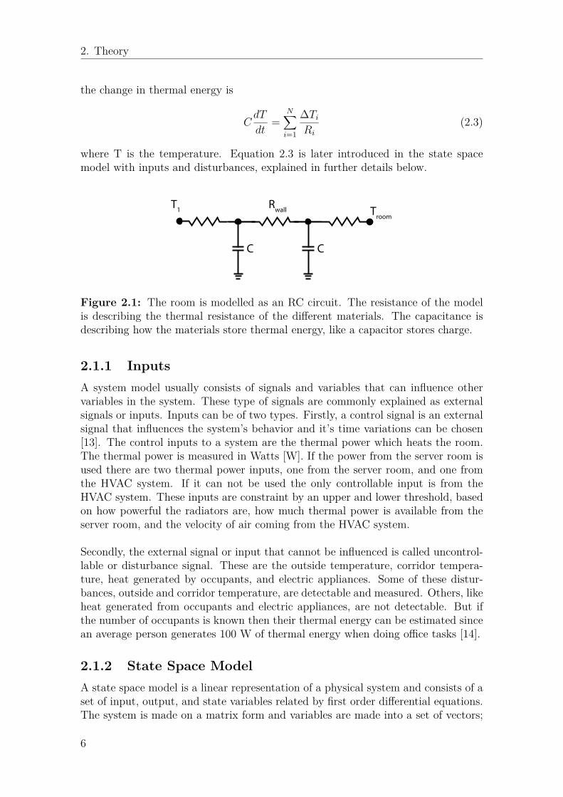
This chapter describes the theoretical background of three different concepts. Itstarts with a general overview the physical modelling of a room. Room modellingconsists of inputs, disturbances and state space models. Furthermore, a general ideaof a Heat Ventilation and Air Condition (HVAC) system is presented. The HVACsystem is what regulates the temperature and ensures air quality in a building.The chapter then finishes with explaining how MPC works by explaining recedinghorizon, objective function, and optimization. The purpose of these sections is togive the reader an introduction to the concepts and its scientific status in relationto this thesis in order to be able to interpret and understand the results.

2.1 Room modelling

Room modelling is about representing and describing a physical room as a mathe-matical model. Equations and formulas can predict how various devices will behavein response to the inputs to these devices [12]. There are many reasons why onewould want to represent a physical room as a mathematical model, e.g. to predicttemperature in a room. When predicting a temperature in a room, one way tomake such a prediction is to describe the room as an RC-circuit. Figure 2.1 shows asimplified circuit of the system. The resistance in the circuit is the materials whichthermal energy flows through, e.g. walls and windows. The resistance for eachmaterial is described as

Ri = wiAiki

(2.1)

where R is the resistance, i is the ith material, w the width of the material, A thearea, and k a thermal conductivity coefficient. The storage of thermal energy ismodeled with a capacitor. Examples of energy storage materials are air, walls, andwindows. The capacitance is described as

Ci = micpi (2.2)

where C is the capacitance, m is the mass of the material, and cp is the specific heatcapacity of the material.

Without external inputs and disturbances the first order differential equation for

5

2. Theory

the change in thermal energy is

CdT

dt=

N∑i=1

∆TiRi

(2.3)

where T is the temperature. Equation 2.3 is later introduced in the state spacemodel with inputs and disturbances, explained in further details below.

Rwall

CC

T1 Troom

Figure 2.1: The room is modelled as an RC circuit. The resistance of the modelis describing the thermal resistance of the different materials. The capacitance isdescribing how the materials store thermal energy, like a capacitor stores charge.

2.1.1 InputsA system model usually consists of signals and variables that can influence othervariables in the system. These type of signals are commonly explained as externalsignals or inputs. Inputs can be of two types. Firstly, a control signal is an externalsignal that influences the system’s behavior and it’s time variations can be chosen[13]. The control inputs to a system are the thermal power which heats the room.The thermal power is measured in Watts [W]. If the power from the server room isused there are two thermal power inputs, one from the server room, and one fromthe HVAC system. If it can not be used the only controllable input is from theHVAC system. These inputs are constraint by an upper and lower threshold, basedon how powerful the radiators are, how much thermal power is available from theserver room, and the velocity of air coming from the HVAC system.

Secondly, the external signal or input that cannot be influenced is called uncontrol-lable or disturbance signal. These are the outside temperature, corridor tempera-ture, heat generated by occupants, and electric appliances. Some of these distur-bances, outside and corridor temperature, are detectable and measured. Others, likeheat generated from occupants and electric appliances, are not detectable. But ifthe number of occupants is known then their thermal energy can be estimated sincean average person generates 100 W of thermal energy when doing office tasks [14].

2.1.2 State Space ModelA state space model is a linear representation of a physical system and consists of aset of input, output, and state variables related by first order differential equations.The system is made on a matrix form and variables are made into a set of vectors;

6

2. Theory

state, input, and output. The general state space model expression of a linear systemis written in the following form:

x(t) = Ax(t) +Bu(t) +Bdud(t)

y(t) = Cx(t) +Du(t)

where x(t) is the state vector, x is the derivative of the state vector, u(t) is theinput vector, ud(t) the disturbances, and y(t) is the output vector. The matricesA,B,C,D relate the state and input vectors to the state derivative and output [13].In this thesis work the A matrix relates to how energy flows through the rooms.The B matrix describes how the input effects the temperature in the rooms. The Cmatrix tells how the measurements relates to the states. D relates to how the inputeffects the measured output.

7

2. Theory

2.2 HVAC systemA heating, ventilation, and air conditioning system is used to provide comfortabletemperature and decent air quality indoors [15]. It consists of an inlet fan and anexhaust fan which provide the air circulation in the system. It also includes damperswhich open and close depending on how much air should go through the dampers,and the velocity of the air. Also, there are heating and cooling coils that heat orcool the air in the duct and lastly, the system includes filters that filter the air.

A typical HVAC system pumps air from the outside and into the system, where itis filtered and mixed with air already in circulation. Next the air passes throughcoils that heat and/or cool the air to the desired temperature for the air duct. Theair is then pumped by a fan into the air duct where it travels to the zones in thebuilding that must be supplied with air. At each zone is a reheating coil whichensures that the air entering the zone is within the thermal comfort level. To keepthe air circulating, another fan pumps the air out of the room. The majority of airpumped out of the rooms is mixed with the incoming air, but the same amount ofincoming air is released out into the atmosphere. Figure 2.2 shows how a simpleHVAC system looks like where zone 1 and 2 represent two rooms.

Zone 1 Zone 2

SUPPLY FAN

RETURN FAN

HEATING / COOLINGCOLIS

EXHAUST AIR

SUPPLY AIR

DAMPER

Figure 2.2: The main components of an HVAC system

The part of the HVAC system this thesis work focuses on is the thermal energy thatis added to a room and is done by using a MPC.

2.3 Model Predictive Control

Model Predictive Control (MPC) is a control method where an objective function isoptimized based on a set of constraints, within a finite prediction window [7]. Thepredicted future outputs are based on the current input, outputs, and the futurecontrol inputs. As was discussed earlier, the difference between a LQR controllerand a MPC is that LQR has an infinite control horizon but the MPC has a finitehorizon. This is where the concept of a receding horizon is considered.

8

2. Theory

The idea with the receding horizon is to choose the best control signal based onfuture trajectory and constraints. It is described in three steps:

1. At time instant k calculate the process response over the prediction horizonusing a future control sequence.

2. Pick the control sequence which minimizes the objective function and operateswithin the constraints.

3. Apply the first element of the chosen control sequence, discard the rest, andmove to time instant k + 1.

Because of the receding horizon, the current information about the plant is neededfor the prediction. Thus, the input can have no direct effect on the output, makingthe D matrix in the state space model zero [7].

Based on the state space model, the future values of each state can be estimated tospan the duration of the prediction window

x(k + 1|k) = Ax(k) +Bu(k) +Bdud(k)x(k + 2|k) = Ax(k + 1|k) +Bu(k + 1) +Bdud(k + 1)

= A2x(k) + ABu(k) + ABdud(k) +Bu(k + 1) +Bdud(k + 1)...

x(k +Np|k) = ANpx(k) + ANp−1Bu(k) + ANp−1Bdud(k) + ANp−2Bu(k + 1)+ . . .+ ANp−NcBu(k +Nc− 1) + ANp−NcBdud(k +Nc− 1).

These equations are represented in matrix form in Equation (2.4)X = Ψx(k) + ΦU + ΦdUd (2.4)

where

X =

x(k + 1|k)x(k + 2|k)

...x(k +Np|k)

U =

u(k|k)

u(k + 1|k)...

u(k +Nc− 1|k)

Ud =

ud(k|k)

ud(k + 1|k)...

ud(k +Nc− 1|k)

Ψ =

AA2

A3

...ANp

Φ =

B 0 0 · · · 0AB B 0 · · · 0A2B AB B

. . . 0... ... ... ... ...

ANp−1B ANp−2B · · · ANp−Nc−1B ANp−NcB

Φd =

Bd 0 0 · · · 0ABd Bd 0 · · · 0A2Bd ABd Bd

. . . 0... ... ... ... ...

ANp−1Bd ANp−2Bd · · · ANp−Nc−1Bd ANp−NcBd

9

2. Theory

2.3.1 Objective functionThe objective function is the equation that is minimized given some constraints. InEquation 2.5 the objective function is represented as J and constraints are expressedon the following form, see Equations 2.6 and 2.7:

J(x, u) = 12x

TQx+ xTF + 12u

TRu+ uTE (2.5)

Mx ≤ b (2.6)

Nu ≤ γ (2.7)Where Q and R are design matrices relating to the quadratic part of the objectivefunction. Q includes the weights put on the states, and R includes the weights forthe inputs. F and E are also weight matrices for the states and inputs, but arerelating to the linear terms of the objective function. M is a matrix that relatesto the constraints of the states and b is the constraint vector. N is a matrix thatrelates to the constraints of the inputs, and γ is the input constraint vector.

Two different objective functions are considered, one quadratic and one linear. Thequadratic function is considered for the reference tracking and the linear when theenergy usage from the HVAC system is minimized. When the quadratic case isconsidered, the objective function is related to the state and how close it is to areference value. That means that when the state is far from the reference value theresult from the objective function will be high. The reference value acts as a steadystate. Thus, the input value that minimizes that difference is ∆u(k) = u(k)− uss ,which is the deviation from the input which gives the steady state. Let r(k) denotethe reference value at time k, S the weight matrix on the output, and C the outputmatrix from the state space.

J(x, u) = 12(r(k +Np)− Cx(k +Np))TS(r(k +Np)− Cx(t+Np))

+ 12

Np−1∑i=0

[(r(k+ i)−Cx(k+ i))TS(r(k+ i)−Cx(t+ i)) + ∆uT (k+ i)R∆u(k+ i)

](2.8)

Rewriting in terms of the full horizon and ignoring the constant terms, Equa-tion (2.8) becomes

J(x, u) = 12U

T (ΦT QΦ + R)U +[x(k)T r(k)T

] [ΨT QΦ−TΦ

]U (2.9)

where Q, R and T are

Q =

Q

. . .Q

S

R =

R

. . .R

R

T =

QC

. . .QC

SC

10

2. Theory

and Q is a positive semi-definite matrix and R is a positive definite matrix.The disturbance is not taken into account because the reference value r is the steadystate value xss, which means that the disturbance cancels out

x(k + 1)− r(k + 1) = Ax(k) +Bu(k) +Bdud(k)− (Axss +Buss +Bdud(k)).

For the linear case, when the energy from the HVAC system is minimized, theobjective function is seen in Equation (2.10)

J(x, u) = fT [x, u]T (2.10)where f is a vector which corresponds to the variables that should be optimized.

2.3.2 OptimizationThe optimization used in this thesis work is called convex optimization. It minimizesconvex functions over a convex set. A convex set (C) is one where a line can bedrawn between any two points a, b within the set and the line is also within the set.A mathematical representation of this can be seen below:

a, b ε C, θ ε [0, 1] =⇒ θa+ (1− θ)b ε C, ∀a, bεC.The convex set is bounded by the constraints on the system. If the set is not convex,there might not exist a minimum for the objective function. A convex function isa function that curves upwards, e.g. f(x) = x2. Due to the upward curve, theminimum found in the optimization is a global minimum. A function that curvesdownward, e.g. f(x) = −x2, is called a concave function. A function is convex if itsHessian matrix is positive semi-definite.

The linear objective function previously discussed in section 2.3.1 is a special caseof a convex function where the Hessian matrix is zero. An example of both cases isshown in Figure 2.3.

f(x)f(x)

C C

X

Y

X

Y

Figure 2.3: The figure shows both a linear function and a quadratic function withina convex set.

11

2. Theory

12

3Methods

The initial step in the thesis work was to find use for the data and sensors, andexplore in which areas the data could be used. After reviewing the sensor data,it became clear that the temperature in all meeting rooms in Ericsson’s offices inGothenburg were being controlled to a set-point value. The temperature fluctuatedaround 21.5◦C regardless of the time of day, or if a room was occupied. This iswhere the premise of the problem formulation was formed. By making the temper-ature in the room dependent on occupation, rather than on a fixed set-point value,energy consumption could be reduced. Therefore, a controller which was capable oflimiting energy usage, while keeping the temperature within a set of constraints hadto be implemented. The controller chosen was a MPC. To implement the MPC, astate space model had to be constructed. It accounted for the thermal dynamics ofthe rooms, and incorporated the disturbances to the rooms. To further the energysavings the thermal power generated by Ericsson’s server rooms was considered asan alternative heat source to the meeting rooms. The idea was to reduce the wasteof pumping out the warm air in the server rooms, while heating air from the outsideto warm the meeting rooms. To limit the scope of the problem, two identical roomswere chosen to share one MPC. The two rooms are subjected to disturbances fromthe outside, the adjacent room and corridor, and people.

The following sections derive the state space model and the MPC implementationin detail.

3.1 State Space Modelling

The thesis work focuses on two rooms that lie next to one another and share onewall. An overview is seen in Figure 3.1. The figure shows the direction of heat flow,indicated by the black arrows, which is needed to derive the state space model. Thered arrows indicate the input to the system, and the blue arrows are the thermalpower which is subtracted from the room.

13

3. Methods

ROOM 1

Corridor

ROOM 2

Outside

q1serverq1hvac q2serverq2hvac

q12

q1out q2out

q1corridor q2corridor

Figure 3.1: Two dimensional view of the room layout. The black arrows indicatethe direction of heat flow. The colored arrow indicate the thermal power beingadded to or removed from the rooms.

The state space matrix is set up by deriving the mathematical equations based onFigure 3.1. Using the following steps the system in Equation (3.1) is acquired.

C1dT1

dt= q1server + q1hvac︸ ︷︷ ︸

inputs

− q12 − qout − qcorridor + qpeople1︸ ︷︷ ︸disturbances

= q1server + q1hvac + qpeople −T1 − T2

R12− T1 − TC

RC1

− T1 − TO1

RO1

= q1server + q1hvac + qpeople −1R1T1 + 1

R12T2 + 1

RC

TC + 1RO1

TO

dT1

dt= 1C1

(q1server+q1hvac+qpeople)−1

C1R1T1+ 1

C1R12T2+ 1

C1RC

TC+ 1C1RO1

TO (3.1)

The state equation for the right room is derived the same way, but there q12 has apositive sign. When the thermal power from the server room is not applied, qserveris disregarded.Setting the state equations for both rooms on a state space form yields the followingsystem

[T1T2

]︸ ︷︷ ︸

˙x(t)

=[− 1C1R1

1C1R121

C2R12− 1C2R2

]︸ ︷︷ ︸

A

[T1T2

]︸ ︷︷ ︸x(t)

+[ 1C1

0 1C1

00 1

C20 1

C2

]︸ ︷︷ ︸

B

q1hvacq2hvacq1serverq2server

︸ ︷︷ ︸

u(t)

+[ 1C1RC 1

1C1RO1

1C1

01

C2RC 21

C2RO20 1

C2

]︸ ︷︷ ︸

Bd

TCTO

qpeople1

qpeople2

︸ ︷︷ ︸

ud(t)

14

3. Methods

[T1T2

]︸ ︷︷ ︸y(t)

=[1 00 1

]︸ ︷︷ ︸

C

[T1T2

]︸ ︷︷ ︸x(t)

3.1.1 Numerical values

To calculate the numerical coefficients in the state space model the physical param-eters of the room and its objects is considered. These parameters are related to thesize of the room, the thermal capacitance, and the thermal resistance. Tables 3.1and 3.2 show the dimension of the rooms and parametric values of the materials.

Table 3.1: Room and window dimensions in meters

Width [Bwi] Height [Bhi] Length [Bli]Room 1 2.7 2.7 2.3Room 2 2.7 2.7 2.3

Window Width [Wwi] Window Height [Whi] Window Length [Wli]Room 1 0.02 1.5 2.3Room 2 0.02 1.5 2.3

Table 3.2: Different heat capacity, thermal conductivity, density and width of thedifferent materials.

Window glass Sand Plaster Cement Aircp [J/kg·m3] 840 [16] 900 [16] 1550 [16] 1005 [17]k [W/m·K] 0.96 [18] 0.71 [18] 0.29 [18] 0.026 [18]ρ [kg/m3] 2500 [19] 801 [20] 1522 [20] 1.225 [20]

w [m] 0.02 0.05 0.2

The dimensions of the room, presented in Table 3.1, make it possible to calculate theareas of the heat flow. The heat flow to the rooms depends on the area of contactand temperature at the other side of the material. Figure 3.1 shows the layout ofthe rooms and their surroundings. Table 3.3 shows the areas of the different heatflows.

15

3. Methods

Table 3.3: Contact areas for the different heat flows in both rooms.

Zone Area [m2]Room 1 to Outside [A1O] Bw1Bh1 −Wl1Wh1Room 2 to Outside [A2O] Bw2Bh2 −Wl2Wh2Room 1 to Room 2 [A12] Bl1Bh1Room1 to Corridor [A1C ] Bw1Bh1 +Bl1Bh1Room2 to Corridor [A2C ] Bw2Bh2 +Bl2Bh2

Window 1 [AW1] Wl1Wh1Window 2 [AW2] Wl2Wh2

The thermal resistance is what hinders the thermal flow from a room the anotherside of it. The resistances differ based on the material, and its area. When an areaconsists of two or more different materials, like a wall with window, its resistanceis calculated by the parallel connection of the materials. Table 3.4 shows how theresistances for all the areas are calculated, as well as how R1 and R2 from the statespace model are derived.

Table 3.4: The table shows how the each of the thermal resistances is calculated.

Outside resistance [ROi](kconcreteAiO

wconcrete+ kwindowAWi

wwindow

)−1

Corridor resistance [RCi]wplaster

AiCkplaster

Room 1 to Room 2 [R12] wplasterA12kplaster

R1 ( 1RO1

+ 1RC1

+ 1R12

)−1

R2 ( 1RO2

+ 1RC2

+ 1R12

)−1

The thermal capacitance is a materials ability to hold on to thermal energy, like acapacitor in an electric circuit can hold on to charge. The capacitance is calculatedby multiplying the specific heat capacity of a material (cp) with the material’s mass.Each material is subjected to a single thermal flow. Hence the materials act like aparallel circuit of capacitors. Therefore the total heat capacity of a room is the sumof the capacitance of each material. Table 3.5 shows how the mass for each materialis calculated, as well as the capacitance.

Table 3.5: The mass and capacitance for the different materials and rooms.

mairi ρairBwiBhiBli

mconcretei ρconcreteAiOwconcretemglassi ρglassAiOwglass

mplasteri ρplasterAiOwplasterC1 cpairmair1 + cpconcretemconcrete1 + cpglassmglass1 + cpplastermplaster1C2 cpairmair2 + cpconcretemconcrete2 + cpglassmglass2 + cpplastermplaster2

16

3. Methods

3.1.2 DiscretizationWhen the model had been numerically derived the next step was to make the modeldiscrete, since the MPC is a digital algorithm. The sampling time was chosen as10 minutes. It was chosen due to the dynamics of an office building, and at whichintervals meeting rooms could be booked. When a system is made discrete thefollowing calculations are made

Ad = eAcTs , Bd =∫ Ts

0eAcτdτBc = A−1

c (Ad − I)Bc, Cd = Cc

where the subscript d stands for discrete, the subscript c stands for continuous, andTs is the sampling time. These calculations can be simplified by using a first orderTaylor expansion. The matrices then become

Ad ≈ I + AcTs

Bd ≈ A−1c (I + AcTs − I)Bc = TsBc.

which makes them easy to implement in Matlab. The reason why a first order Taylorexpansion is used to make the model discrete instead of other methods, is to keepthe B matrix so that the inputs in one room does not effect the other [9], and thedynamics of the system are very slow.

3.1.3 Server RoomThe server room is modeled after a general sized server room in a large office buildinglocated in colder climate. A general layout of the server room describing the heatflow can be seen in Figure 3.2 and the dimensions and specifications of the roomcan be seen in Table 3.6.

Corridor

SERVER ROOM

qcorridor

qIN qOUT

qservers

Figure 3.2: Two dimensional layout of larger server room with theoretical energyflows.

17

3. Methods

Table 3.6: Specification of room dimensions, quantity and type of servers.

Server Room SpecificationsRoom Dimensions Height [Rhi] 2.3 [m]

Width [Rwi] 10.0 [m]Length [Rle] 10.0 [m]Wall Thickness [Rth] 0.2 [m]

Room Windows Height [Whi] 1.2 [m]Width [Wwi] 10.0 [m]Window Thickness [Wth] 0.02 [m]

Servers Number of servers [nservers] 600Number of racks [nracks] 30Mass of rack with servers [mservers] 400 [kg]System Heat/Power 121 [W]Operational Temperature [TSmin, TSmax] 20 - 38 [C°]Server Type Dell PE860Processor Type Xeron 3070

In reality the server room consist of multiple server types but for simulation purposesa single type commonly used server was selected to represent the the heat generation.The heat admittance is mainly dependent on on server workload and is scalabledue to its linear characteristics. The room have been modeled using the same RC-circuit description as the meeting room with the resistance and capacitance variablespresented in Table 3.7.

Table 3.7: Server room surface area, mass, capacitance and resistance.

Awindow WwiWhi

Awalls 4RwiRhi − Awindowmair,room ρairRwiRhiRle

mwalls ρcementAwallsRth

mwindows ρglassAwindowWth

CS cpairmair + cpconcretemconcrete + cpglassmwindows + cpsteelmracknracks

RS

(kconcreteAwallsRth

+ kwindowAwindowWth

)−1

The server room is located within the Ericsson building with no wall facing theoutside. All walls connect to an inner corridor regulated at around 22°C, withone of the walls consisting mainly of a large window according to Figure 3.2. Thematerial of the walls are concrete and the servers are mostly steel. The temperaturein the room is regulated by the energy flow qin and qout which is controlled by aseparate dedicated server room HVAC system, different from the one governing themeeting rooms. The disturbance of the system is attributed to surrounding corridortemperature Tcorridor and the energy being generated by the servers qservers. The

18

3. Methods

server room state space model below is constructed in a simular way as for themeeting rooms with TS being the change in temperature of the server room:

[TS]

=[− 1CSRS

] [TS]

+[

1CS− 1CS

] [ qinqout

]+[

1RSCS

1CS

] [Tcorridorqservers

]

Using Dell’s own tool called Datacenter Capacity Planner [21] the maximum com-bined estimated heat output from the servers was calculated to qs,max = 72, 6 KJ/sfor this particular server setup. The server processor utilization is represented usinga sine wave function see Equation 3.2 with the energy output being the productof utilization percentage and maximum capacity. The variation is set to fluctuatebetween 20 − 100% utilization of maximum capacity to represent average normalusage, assuming a greater server load during office hours and a lower demand therest of the day and during weekends.

qserver(k) = qs,maxsin(0.044k + 0.1) + 0.6

2.5 (3.2)

The server room state space representation derived from the RC-circuit descriptionis used to simulate how much energy the server room generates in an active statewhile maintaining a acceptable operational temperature specified by the servers.The HVAC control of the server room is regulated using linear programming opti-mization. Minimizing the input energy being used while keeping the room withinacceptable temperature limits and generating maximum energy output. Server roomcontrol is realized using the Matlab function linprog() in a similar way as describedin Section 3.2.3. The lower bound for the input energy is set to 100W with no upperbound for energy output:[

−ΦΦ

]︸ ︷︷ ︸Ain

U ≤[−TSmin + ΨT (k) + ΦdUdTSmax −ΨT (k)− ΦdUd

]︸ ︷︷ ︸

Bin

The resulting input control signal Qout is considered to be the available energyoutput from the room since it is the minimum energy export needed to maintain anoperational temperature of below 38◦C. In Figure 3.3 the available energy from theserver room, later to be used by the MPC is presented.

0 100 200 300 400 500 600 700 800 900 1000

Time [10 m]

0

2

4

6

8

Po

we

r [W

]

104 Server Room

Figure 3.3: Output energy of server room being regulated at a constant tempera-ture of 38◦C over a 7 day period.

19

3. Methods

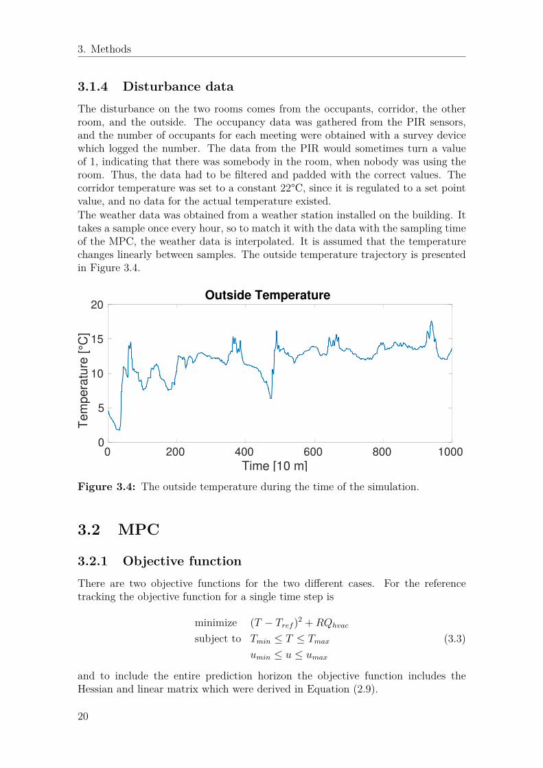
3.1.4 Disturbance dataThe disturbance on the two rooms comes from the occupants, corridor, the otherroom, and the outside. The occupancy data was gathered from the PIR sensors,and the number of occupants for each meeting were obtained with a survey devicewhich logged the number. The data from the PIR would sometimes turn a valueof 1, indicating that there was somebody in the room, when nobody was using theroom. Thus, the data had to be filtered and padded with the correct values. Thecorridor temperature was set to a constant 22°C, since it is regulated to a set pointvalue, and no data for the actual temperature existed.The weather data was obtained from a weather station installed on the building. Ittakes a sample once every hour, so to match it with the data with the sampling timeof the MPC, the weather data is interpolated. It is assumed that the temperaturechanges linearly between samples. The outside temperature trajectory is presentedin Figure 3.4.

0 200 400 600 800 1000

Time [10 m]

0

5

10

15

20

Te

mp

era

ture

[°C

]

Outside Temperature

Figure 3.4: The outside temperature during the time of the simulation.

3.2 MPC

3.2.1 Objective functionThere are two objective functions for the two different cases. For the referencetracking the objective function for a single time step is

minimize (T − Tref )2 +RQhvac

subject to Tmin ≤ T ≤ Tmax

umin ≤ u ≤ umax

(3.3)

and to include the entire prediction horizon the objective function includes theHessian and linear matrix which were derived in Equation (2.9).

20

3. Methods

For the linear case the objective is to minimize the energy used by the HVAC system.Thus the function for a single time step is

minimize qhvac1 + qhvac2

subject to Tmin ≤ T ≤ Tmax

umin ≤ u ≤ umax

(3.4)

and to include the entire horizon, fT from equation (2.10) becomes

fT =[1 1 0 0 . . . 1 1 0 0

].

When the objective functions had been implemented for the entire prediction hori-zon, the same had to be done for the constraints.

3.2.2 Constraints

The constraints that the MPC must operate within relate to the temperature in theroom, and the thermal power used to control the temperature. The constraints onthe temperature are dependent on the occupancy status on the room. If nobodyis in the room the temperature range is between 15◦C and 29◦C, and when theroom is occupied the temperature must be within 21◦C and 24◦C. The constraintsvalues when a room is occupied is chosen because temperature outside of that rangeaccounts for 96.5% of temperature complaints in commercial buildings [14]. Thisis incorporated in the MPC algorithm by adding a slack variable s(k). The slackvariable is added to form a soft constraint. This is due to the fact that outputconstraints can cause large changes in the control, which can yield the input variablesto violate their constraints [7]. The slack variable is activated 4 time samples beforea meeting starts. For each time step the change in the constraints is 1◦C, until thelower bound is 21◦C, and the upper bound is 24◦C.The constraints on the power used from the server room is constrained by the allowedtemperature of the air that comes in to the room by the HVAC system. The otherconstraints on the inputs are for the radiators. The power from them can rangebetween 0 W and 6000 W. However, due to the continuous circulation of the HVACsystem, the minimum thermal power going in must be at least equal to the flow ofair going in to the room at duct temperature. The duct temperature is consideredconstant at 10°C. Since the air does not need to be heated to 10°C, this minimuminput is deducted from the total energy consumption. The MPC can choose not touse any power from the server room, which means that the lower limit is 0 W. Theupper limit depends on the thermal load that the servers produce, which varies.When the objective function includes reference tracking the power from the serverroom is not considered. This changes the constraints. Table 3.8 shows the con-straints for both objective functions.

21

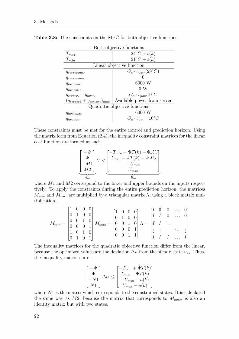
3. Methods

Table 3.8: The constraints on the MPC for both objective functions

Both objective functionsTmax 24◦C + s(k)Tmin 21◦C + s(k)

Linear objective functionqservermax Ga · cpair(29◦C)qservermin 0qhvacmax 6000 Wqhvacmin 0 Wqserveri

+ qhvaciGa · cpair10◦C

(qserver1 + qserver2)max Available power from serverQuadratic objective functions

qhvacmax 6000 Wqhvacmin Ga · cpair · 10◦C

These constraints must be met for the entire control and prediction horizon. Usingthe matrix form from Equation (2.4), the inequality constraint matrices for the linearcost function are formed as such

−ΦΦ−M1M2

︸ ︷︷ ︸

Ain

U ≤

−Tmin + ΨT (k) + ΦdUdTmax −ΨT (k)− ΦdUd

−UminUmax

︸ ︷︷ ︸

Bin

where M1 and M2 correspond to the lower and upper bounds on the inputs respec-tively. To apply the constraints during the entire prediction horizon, the matricesMmin and Mmax are multiplied by a triangular matrix Λ, using a block matrix mul-tiplication.

Mmin =

1 0 0 00 1 0 00 0 1 00 0 0 11 0 1 00 1 0 1

Mmax =

1 0 0 00 1 0 00 0 1 00 0 0 10 0 1 1

Λ =

I 0 0 . . . 0I I 0 . . . 0I I

. . .... ... ... . . . ...I I I . . . I

The inequality matrices for the quadratic objective function differ from the linear,because the optimized values are the deviation ∆u from the steady state uss. Thus,the inequality matrices are

−ΦΦ−N1N1

∆U ≤

−Tmin + ΨT (k)Tmin −ΨT (k)−Umin + u(k)Umax − u(k)

where N1 is the matrix which corresponds to the constrained states. It is calculatedthe same way as M2, because the matrix that corresponds to Mmax, is also anidentity matrix but with two states.

22

3. Methods

3.2.3 Matlab ImplementationFor the linear objective function the Matlab function linprog() is used with thedual-simplex algorithm. It takes in the f vector which corresponds to the inputsthat are minimized, and the inequality matrices Ain and bin. The Dual Simplex isa linear programming algorithm which performs a simplex algorithm. A simplexalgorithm looks for the optimum value by evaluating the objective function at thevertices of a set, which are made by the constraints. It iteratively updates the ver-tex set until the solution does not improve in any direction, which means that theoptimum is found [22].

For the quadratic objective function the Matlab function quadprog() is used withthe interior point convex algorithm. It takes in the Hessian matrix H and F T fromEquation (2.9), along with the inequality matrices Ain and bin The interior pointconvex algorithm performs five steps [23].

1. Presolve/Postsolve. The problem is simplified, redundancies removed, and theconstraints simplified.

2. Generate Initial Point3. Predictor-Corrector. The inequalities are put on a different form, and a point

where the KKT conditions are met is found.4. Stopping Conditions5. Infeasibility Detection

For the quadratic case the steady state value of the input must be calculated. Thedisturbance changes this value, so it must be calculated for every time step. It isdone the following way [

xssuss

]=[I − A −BC 0

]−1 [Bdud(k)

r

]

and to get the next control input the first values from quadprog() are added touss.

23

3. Methods

24

4Results

This chapter shows the results from the simulations. The results from the tworooms are presented in a separate sections, where each section includes results fromboth the quadratic and linear objective functions. Lastly, the total usage in kWh ispresented. The results are acquired by simulating one week of data. During thatcourse Room 1 is occupied for 280 minutes, and Room 2 is occupied for 730 minutes.The controllers have a prediction and control horizon that checks 6 time steps ahead,or 1 hour. The initial conditions are set to 22°C in both rooms. The reference valuein the rooms was set to 21.5°C.

4.1 Room 1

0 500 1000

Time [10 m]

21.2

21.4

21.6

21.8

22

Temp

eratu

re

Quadratic Objective Function Room 1

Temperature

Reference Temperature

Figure 4.1: The temperature in room 1 for the quadratic objective function

25

4. Results

0 500 1000

Time [10 m]

0

1000

2000

3000

Pow

er

[W]

Quadratic Objective Function Room 1

Room 1

Figure 4.2: The thermal power usage for room 1

0 500 1000

Time [10 m]

15

20

25

30

Tem

pera

ture

Room 1

Temperature

Lower limit

Upper limit

Figure 4.3: The temperature in room 1 for the occupancy based constraints

26

4. Results

0 500 1000

Time [10 m]

0

200

400

600

800

1000

1200

Po

we

r [W

]

HVAC energy Room 1

Figure 4.4: The HVAC energy usage in room 1 for the occupancy based constraints

0 500 1000

Time [10 m]

500

1000

1500

2000

2500

3000

Po

we

r [W

]

Server room energy Room 1

Figure 4.5: The thermal power from the server room provided to room 1 for theoccupancy based constraints

27

4. Results

4.2 Room 2

0 500 1000

Time [10 m]

21.2

21.4

21.6

21.8

22

Te

mp

era

ture

Quadratic Objective Function Room 2

Room 2

Figure 4.6: The temperature in room 2 for the quadratic objective function

0 500 1000

Time [10 m]

0

1000

2000

3000

Po

wer

[W]

Quadratic Objective Function Room 2

Room 2

Figure 4.7: The thermal power usage for room 2

28

4. Results

0 500 1000

Time [10 m]

15

20

25

30

Tem

pera

ture

Room 2

Temperature

Lower limit

Upper limit

Figure 4.8: The thermal power from the server room provided to room 2 for theoccupancy based constraints

0 500 1000

Time [10 m]

0

200

400

600

800

Po

we

r [W

]

HVAC energy Room 2

Figure 4.9: The HVAC energy usage in room 2 for the occupancy based constraints

29

4. Results

0 500 1000

Time [10 m]

0

1000

2000

3000

Po

we

r [W

]

Server room energy Room 2

Figure 4.10: The server energy usage in room 2 for the occupancy based constraints

4.3 Numerical resultsAfter accounting for the duct temperature, the total kWh for both cases are calcu-lated and presented in Table 4.1.

Table 4.1: Results for one week of use

kWh from HVAC kWh from server room TotalQuadratic objective function

Room 1 83.9 83.9Room 2 81.6 81.6Total both rooms 167.5

Linear objective functionRoom 1 1.0 10.3 11.3Room 2 0.8 1.0 1.8Total both rooms 13.1

30

5Discussion

This chapter discusses and interprets the results, addresses the limitations, andrecommendations for future research.

5.1 Comparison between the quadratic and linearMPC

The results show that the total energy usage of the MPC which uses the linearobjective function is only 7.8% of the energy usage by the MPC which uses thequadratic objective function. The energy where the HVAC system is activated isonly 1.8 kWh. Analyzing the plots, it can be seen that the heating from the HVACsystem is only activated before a meeting occurs. The reason for this big differenceis due to the fact that the quadratic MPC has to use energy to stay near the ref-erence value. The linear MPC can input the minimum required temperature whenthe room is unoccupied.

Considering that the rooms are occupied 3% and 7% for Room1 and Room2 respec-tively during a week, it is hard to justify having a controller with a fixed referencevalue, when the objective is reducing energy consumption.

The results show that the controller has a good potential to lower the energy usefrom a building. By implementing such a controller a win-win situation is generatedwhere carbon emission, and the operating cost of a building are both reduced. Evenif a building does not have a server room which generates so much excess thermalpower, the total energy usage is still far lower than for the set-point controller.

5.2 LimitationsCertain assumptions and simplifications were made in this thesis work. Instead thanfocusing on the entire Ericsson office, 2 rooms were chosen to model and control.The reason was to be able to get results during the duration of the thesis project.The theory for the room modelling, and MPC is fundamentally the same when ap-plied on a big scale. However, it was assumed that the two rooms had could utilizeall the thermal power generated by the servers. In reality, each server room couldprovide thermal power to multiple rooms.

31

5. Discussion

Another assumption was that it was known when people would be in the rooms.In reality, people do not always book a room beforehand, which could result in thetemperature in a room to be outside of the thermal comfort zone.

It was assumed that all occupants created the same amount of thermal power. Thatis not true, and how much each person produces is dependent on height, weight, andmetabolic rate.

5.3 Future WorkWhen the MPC is implemented on a larger scale, e.g. an office building, having acentral MPC is not feasible because of the computational complexity. A solutionto that is to do a distributed controller that would control a few rooms or even asingle room. Then every room would have control over itself, and the computationalcomplexity is reduced immensely.

Using the thermal capacitance properties of the room could be utilized so thata it can be "charged" with thermal power when there is excess of it, or when energyprices are low.

There are more disturbances that effect the temperature in the room than are men-tioned in this thesis work, e.g. solar radiation. These disturbances are observable,like the thermal power from the occupants. These disturbances can be estimatedwith an observer.

Storing the thermal energy in a water tank would be a good idea, energy can bekept there and the heat fluctuations in the server room would be limited.

32

6Conclusion

The objective of this thesis was to make a MPC that uses thermal power generated byservers in another part of the same building, while satisfying a number of constraints.The MPC that is implemented is compared to a controller which has a referencevalue at 21.5◦C. The energy usage of the two controllers is then compared. Anotherdifference between the two controllers is that the one which uses thermal powerfrom the servers also has different constraints. When nobody is scheduled to use theroom the temperature range is wider than when the room is occupied. The resultsfrom both controllers were acquired from simulation, and the same data was used inboth cases. The data spans a week, and includes weather and occupation data. Thecontroller proposed in this thesis work only used 7.8% of the energy compared to thecontroller using the reference value. Thereof, the majority of energy was providedby the excess thermal energy from the server room. The thesis work shows thatcommercial buildings have the potential of reducing their energy usage greatly byusing the proposed controller.

33

6. Conclusion

34

Bibliography

[1] P. Huovila, M. Alla-Juusela, L. Melchert, and S. Pouffary, “Build-ings and climate change: Summary for Decision-Makers,” Tech. Rep.,2007. [Online]. Available: https://europa.eu/capacity4dev/unep/document/buildings-and-climate-change-summary-decision-makers

[2] L. Pérez-Lombard, J. Ortiz, and C. Pout, “A review on buildings energy con-sumption information,” Energy and Buildings, 2008.

[3] I. E. A. IEA, “Energy Efficiency Indicators Highlights (2017 edition),” Inter-national Energy Agency, 2017.

[4] Ericson, “Ericsson Sustainability Policy,” 2014. [Online].Available: https://www.ericsson.com/assets/local/about-ericsson/sustainability-and-corporate-responsibility/documents/sustainability-policy.pdf

[5] Mathworks, “MATLAB - Mathworks - MATLAB & Simulink,” 2016.[6] Ruchika and R. Neha, “Model Predictive Control: History and Developement,”

International Journal of Engineering Trend and Technology (IJETT), vol. 4,no. 6, pp. 2600–2602, 2013. [Online]. Available: http://www.ijettjournal.org/volume-4/issue-6/IJETT-V4I6P173.pdf

[7] L. Wang, Model Predictive Control System Design and Implementation UsingMATLAB, 2009.

[8] A. Afram and F. Janabi-Sharifi, “Theory and applications of HVAC controlsystems - A review of model predictive control (MPC),” 2014.

[9] K. Carstaedt, “Distributed Model Predictive Control for Building TemperatureControl,” Master’s thesis, Lund University, 2016.

[10] F. Oldewurtel, A. Parisio, C. N. Jones, D. Gyalistras, M. Gwerder, V. Stauch,B. Lehmann, and M. Morari, “Use of model predictive control and weatherforecasts for energy efficient building climate control,” Energy and Buildings,2012.

[11] S. H. Cho and M. Zaheer-Uddin, “Predictive control of intermittently operatedradiant floor heating systems,” Energy Conversion and Management, 2003.

[12] B. Friedland, Control system design: an introduction to state-space methods.Courier Corporation, 2012.

[13] L. Ljung and T. Glad, Modeling of dynamic systems, 1st ed. Prentice Hall,1994.

[14] ASHRAE, 2013 ASHRAE Handbook: Fundamentals Chapter 9, 2013.[15] Y. Yao and Y. Yu, Modeling and Control in Air-conditioning Systems, 1st ed.

Springer-Verlag Berlin Heidelberg, 2017.

35

Bibliography

[16] “Specific Heat of Solids,” 2018. [Online]. Available: https://www.engineeringtoolbox.com/specific-heat-solids-d_154.html

[17] “Specific Heat Capacities of Air,” 2018. [Online]. Available: https://www.ohio.edu/mechanical/thermo/property_tables/air/air_cp_cv.html

[18] “Thermal Conductivity of common Materials and Gases,” 2018. [Online].Available: https://www.engineeringtoolbox.com/thermal-conductivity-d_429.html

[19] “Density Of Glass,” 2018. [Online]. Available: https://hypertextbook.com/facts/2004/ShayeStorm.shtml

[20] “Densities of Common Materials,” 2018. [Online]. Available: https://www.engineeringtoolbox.com/density-materials-d_1652.html

[21] DELL. (2018). [Online]. Available: https://www.dell.com/html/us/products/rack_advisor_new/

[22] S. G. Nash and A. Sofer, Linear and Nonlinear Programming, 1st ed. McGraw-Hill International Editions, 1996.

[23] “Quadratic Programming Algorithms,” 2018. [On-line]. Available: https://se.mathworks.com/help/optim/ug/quadratic-programming-algorithms.html#bsqspm_

36