Heat Transfer Modeling using ANSYS FLUENTdl.racfd.com/Fluent_HeatTransfer_L05_Radiation.pdf · Heat...
65
© 2013 ANSYS, Inc. March 28, 2013 1 Release 14.5 14.5 Release Heat Transfer Modeling using ANSYS FLUENT Lecture 5 – Radiation Heat Transfer
Transcript of Heat Transfer Modeling using ANSYS FLUENTdl.racfd.com/Fluent_HeatTransfer_L05_Radiation.pdf · Heat...

© 2013 ANSYS, Inc. March 28, 2013 1 Release 14.5
14.5 Release
Heat Transfer Modeling using
ANSYS FLUENT
Lecture 5 – Radiation Heat Transfer

© 2013 ANSYS, Inc. March 28, 2013 2 Release 14.5
Outline
• Radiation modelling theory
• Radiation models in FLUENT
• Surface-to-Surface (S2S)
• Discrete Ordinates (DO)
• Discrete Transfer Radiation Model (DTRM)
• P-1
• Rosseland
• Selecting a radiation model
• Postprocessing
• Conclusions
• Appendix

© 2013 ANSYS, Inc. March 28, 2013 3 Release 14.5
Introduction
• Thermal radiation is emission of energy as electromagnetic waves.
• Thermal radiation can occur in vacuum
• When any object is above absolute zero it emits energy.
• Industrial applications for which FLUENT’s radiation models are used:
• Combustion (gas turbine, boilers, rocket engine, glass furnace, steel reheat furnace)
• Automotive under-hood
• Heating, Ventilation, and Air-Conditioning (HVAC)
• Headlights
• Ultraviolet disinfection (water treatment)
• Glass applications (forming, glass tank)
• Many other high-temperature applications

© 2013 ANSYS, Inc. March 28, 2013 4 Release 14.5
Outline
• Radiation modelling theory
• Radiation models in FLUENT
• Surface-to-Surface (S2S)
• Discrete Ordinates (DO)
• Discrete Transfer Radiation Model (DTRM)
• P-1
• Rosseland
• Selecting a radiation model
• Postprocessing
• Conclusions
• Appendix

© 2013 ANSYS, Inc. March 28, 2013 5 Release 14.5
View Factor; fraction of the diffuse
radiative energy leaving surface i and
arriving at surface j
Surface to Surface (S2S) Model
• Method for non-participating media only
• Only surfaces radiate (zero optical thickness).
• Method based on view factor calculation (Chaparral)
• N equations for N surfaces which can be cast into matrix form as
Emissive power vector Radiosity vector
N×N matrix
EJK
i jA
i
A
jij
ji
i
ij dAdArA
F2
coscos1
jA
jdA
jjn̂r
i
in̂iA
idA

© 2013 ANSYS, Inc. March 28, 2013 6 Release 14.5
Radiation Model
S2S Model Setup Numerical parameters to solve
Define Radiation… Models EJK
View Factors and Clustering

© 2013 ANSYS, Inc. March 28, 2013 7 Release 14.5
Participating Boundary Zones
View Factors and Clustering
S2S – Partial Enclosure Option
• Before performing view factor calculation, deselect surfaces that you don’t need in your view factor calculation
• Unselected surfaces are regarded as black body at the temperature defined in the ‘Non-Participating Boundary Zones Temperature’ panel.

© 2013 ANSYS, Inc. March 28, 2013 8 Release 14.5
Wall
S2S – Partial Enclosure Option 2
• Critical zone: Boundary zone in which radiation is very important
• Select Automatic option first.
• Define the Critical Zone in boundary condition panel
• Compute maximum of distances between critical zone and other zones
• Enter maximum distance of participating zone and the critical zone.
• All zones having a critical zone distance greater than the specified distance will be made non-participating
View Factors and Clustering
Participating Boundary Zones
© 2013 ANSYS, Inc. March 28, 2013 9 Release 14.5
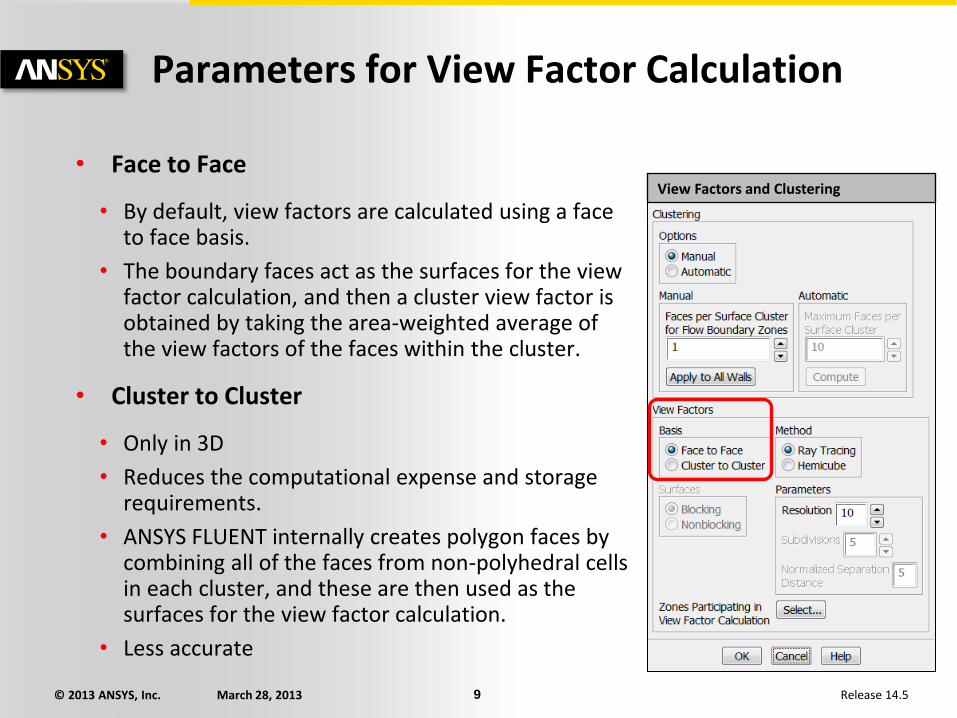
Parameters for View Factor Calculation
• Face to Face
• By default, view factors are calculated using a face to face basis.
• The boundary faces act as the surfaces for the view factor calculation, and then a cluster view factor is obtained by taking the area-weighted average of the view factors of the faces within the cluster.
• Cluster to Cluster
• Only in 3D
• Reduces the computational expense and storage requirements.
• ANSYS FLUENT internally creates polygon faces by combining all of the faces from non-polyhedral cells in each cluster, and these are then used as the surfaces for the view factor calculation.
• Less accurate
View Factors and Clustering

© 2013 ANSYS, Inc. March 28, 2013 10 Release 14.5
Parameters for View Factor Calculation
• Clustering is the built-in capability to group surface faces
• Use fewer surface faces for radiation calculation than flow calculation.
• Reduces only the size of the view factor file
• Calculation process is not faster
Manual
• Faces per surface cluster (FPSC) can be easily specified and applied to all zones
• Any modifications to the FPSC in the critical and non-critical zones need to be done manually.
Automatic
• Calculates FPSC values automatically based on the distance of the zones from other critical zones
• Define the critical zone and specify the minimum FPSC
View Factors and Clustering

© 2013 ANSYS, Inc. March 28, 2013 11 Release 14.5
Parameters for View Factor Calculation
• Blocking / Nonblocking:
• If there is no obstruction between the surface pairs under consideration, then they are referred to as "non-blocking'' surfaces.
• If there is another surface blocking the views between the surfaces under consideration, then they are referred to as "blocking'' surfaces. Blocking will change the view factors between the surface pairs and require additional checks to compute the correct value of the view factors.
View Factors and Clustering

© 2013 ANSYS, Inc. March 28, 2013 12 Release 14.5
Parameters for View Factor Calculation
• Hemicube
• It should be used for complex 3D geometries with few obstructing surfaces between the radiating faces.
• Ray Tracing
• It should be used for complex 3D geometries with lots of obstructing surfaces such as automotive underhood simulations.
View Factors and Clustering

© 2013 ANSYS, Inc. March 28, 2013 13 Release 14.5
Advantages and Disadvantages of S2S
• Advantages
• Once View-Factor calculation is done, low time per iteration
• View-factor calculation is possible in the parallel solver
• Much better accuracy in cases of localized heat sources than DO or any ray-tracing method
• Much smaller memory usage and file storage

© 2013 ANSYS, Inc. March 28, 2013 14 Release 14.5
Advantages and Disadvantages of S2S
• Disadvantages
• The S2S model assumes that all surfaces are diffuse
• The implementation assumes gray radiation
• The storage and memory requirements increase very rapidly as the number of surface faces increases (N x N)
• CPU time is independent of the number of clusters used
• Cannot be used to model participating radiation problems
• Scattering, emission, absorption
• Hemicube view factor methods cannot be used with symmetry boundary conditions
• Does not support non-conformal interfaces, hanging nodes or mesh adaption
• Not strictly conservative

© 2013 ANSYS, Inc. March 28, 2013 15 Release 14.5
• 441,929 tets
• 58,550 shells
• Total: 500,479 cells
• 89,497 boundary faces
S2S Example – Under-Hood Thermal Modeling

© 2013 ANSYS, Inc. March 28, 2013 16 Release 14.5
S2S Example – Under-Hood Thermal Modeling
• STEP 1: Making Partial Enclosure
• Identify those components that have temperature close to "Partial Enclosure Temperature"
• Setting Partial Enclosure Temperature
Radiation Model

© 2013 ANSYS, Inc. March 28, 2013 17 Release 14.5
S2S Example – Under-Hood Thermal Modeling
• STEP 1: Making Partial Enclosure
• Toggle off Participates in S2S Radiation in all the walls (including shadows) that are part of partial enclosure.
Wall

© 2013 ANSYS, Inc. March 28, 2013 18 Release 14.5
–
97282 Faces
46617 Faces
50665 Faces
=
S2S Example – Under-Hood Thermal Modeling

© 2013 ANSYS, Inc. March 28, 2013 19 Release 14.5
S2S Example – Under-Hood Thermal Modeling
• STEP 2: Calculate view factors (outside FLUENT)
• Calculate the cluster file:
• Specify Faces Per Surface Cluster and Set Method to Hemicube
• After writing, verify in Fluent console ratio of radiating faces and clusters is close to what you desire.
File Surface Clusters… Write
View Factors and Clustering
© 2013 ANSYS, Inc. March 28, 2013 20 Release 14.5
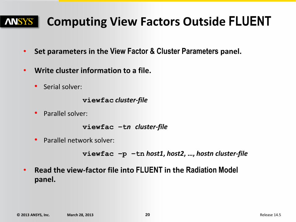
Computing View Factors Outside FLUENT
• Set parameters in the View Factor & Cluster Parameters panel.
• Write cluster information to a file.
• Serial solver:
viewfac cluster-file
• Parallel solver:
viewfac –tn cluster-file
• Parallel network solver:
viewfac –p –tn host1, host2, …, hostn cluster-file
• Read the view-factor file into FLUENT in the Radiation Model panel.

© 2013 ANSYS, Inc. March 28, 2013 21 Release 14.5
S2S Example – Under-Hood Thermal Modeling
• STEP 3: Solve
• Obtain cold-flow solution (first-order, then second-order). Default under-relaxation should be adequate
• Increase Under-Relaxation for Energy to 1.0
• Iterate to convergence
• If Density is not constant:
• Freeze temperature field and solve for flow
• Freeze flow field and solve for energy
• Repeat last two steps until there is no change in residuals or monitored temperatures
• REMEMBER: If view factors calculated outside of FLUENT, you must read in view factors before solving. (FileReadView Factors)

© 2013 ANSYS, Inc. March 28, 2013 23 Release 14.5
Full Enclosure,
Resolution 5
Full Enclosure,
Resolution 10
Full Enclosure,
Resolution 20
DO: 3x3
Partial
Enclosure,
Resolution 5
Partial
Enclosure,
Resolution 10
Partial
Enclosure,
Resolution 20

© 2013 ANSYS, Inc. March 28, 2013 24 Release 14.5
• In absorbing media, it is necessary to take into account some additional terms in the energy equation
• The source term depends on the incident radiation G (sum of each radiation intensity from all the direction over the whole solid angle)
• This characteristic implies that some additional equations have to be solved in order to include the energy source term.
• G equation with P1 method
• I equations (DTRM or DOM)
rTkE
t
ES
V
Participating Media
where 44 TGar q
dIG

© 2013 ANSYS, Inc. March 28, 2013 25 Release 14.5
Radiative Properties of Materials
• All material properties are specified in the Materials panel.
• Absorption
• In combusting flows, the mixture absorption coefficient accounts for the different absorptivities of the species CO2 and H2O and is computed using the Weighted Sum of Gray Gas Model (WSGGM).
• The Domain-Based option is recommend.
• The Cell-Based option is mesh-dependent and should be avoided.
• Soot absorption can also be included.
• The default value for the absorption coefficient is zero.
• Scattering
• With the DO model, a scattering coefficient and phase function are required.
• Scattering is automatically included when one takes into account radiation/particle interactions when using the Discrete Phase Model (DPM).

© 2013 ANSYS, Inc. March 28, 2013 26 Release 14.5
Outline
• Radiation modelling theory
• Radiation models in FLUENT
• Surface-to-Surface (S2S)
• Discrete Ordinates (DO)
• Discrete Transfer Radiation Model (DTRM)
• P-1
• Rosseland
• Selecting a radiation model
• Postprocessing
• Conclusions
• Appendix

© 2013 ANSYS, Inc. March 28, 2013 27 Release 14.5
Discrete Ordinates (DO) Model
• Solves the RTE for a finite number of discrete solid angles, (or directions s)
• The RTE is written on the control volumes (existing mesh) and solved with a finite volume method as opposed to ray tracing method.
• Solves transport equations similar to the flow and energy equations
4
0
42 )(),(
4),(),( dI
TnaIaI s
s sssrsrssr

© 2013 ANSYS, Inc. March 28, 2013 28 Release 14.5
DO – Angular Discretization
• Calculate in each quadrant (2D) or each octant (3D) the RTE for Nθ×Nφ discrete ordinates
• Each DO has a a direction that represents the radiation within a solid angle.
• Solid angle discretization given by Nθ and Nφ
• Azimuthal angle (φ): 0 < φ < 2π
• Polar angle (θ) → 0 < θ < π/2
n
t P
N2
N2
© 2013 ANSYS, Inc. March 28, 2013 29 Release 14.5
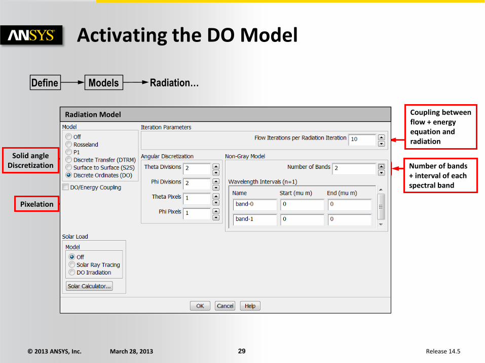
Activating the DO Model
Solid angle Discretization
Coupling between flow + energy equation and radiation
Number of bands + interval of each spectral band
Pixelation
Define Radiation… Models
Radiation Model

© 2013 ANSYS, Inc. March 28, 2013 30 Release 14.5
Solid
DO – Radiation in Solids
• It is possible to compute radiation in solids (such as glass, silica, polymers, etc.)
• Only a thick (meshed) wall (solid zone) will heat up when its material is absorbing radiation.
• For a zero-thickness wall, absorbed energy is calculated but not dissipated. In other words, emitted energy by the volume is not accounted for.

© 2013 ANSYS, Inc. March 28, 2013 31 Release 14.5
Properties of Opaque Surfaces
• Reflectivity, Absorptivity, Emissivity
• Specular and diffuse reflection
Wall
Absorption
Reflection Emission
Diffuse Reflection
Incident
Radiation
Incident
Radiation
Wall
Diffuse
Radiation
Specular Reflection
Wall
eIrI iI
iI
Reflected
Radiation
rI
aI
iI
Incident
Radiation r i
ari III
1
© 2013 ANSYS, Inc. March 28, 2013 32 Release 14.5
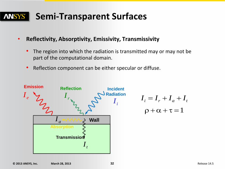
Semi-Transparent Surfaces
• Reflectivity, Absorptivity, Emissivity, Transmissivity
• The region into which the radiation is transmitted may or may not be part of the computational domain.
• Reflection component can be either specular or diffuse.
Wall
Absorption
Reflection Emission Incident
Radiation
Transmission
tari IIII
1
eIrI
iI
aI
tI

© 2013 ANSYS, Inc. March 28, 2013 33 Release 14.5
• Transmitted radiation exits the computational domain
• Diffuse fraction between 0 and 1. (Transmissivity and reflectivity will depend on material properties)
• Incident flux (3 possible choices)
• Solar calculator
• Specified by the user
• Isotropic flux from the environment
Note: Internal emissivity if appearing on the panel is not taken into account for semi-transparent walls
DO – External Semi-Transparent Walls

© 2013 ANSYS, Inc. March 28, 2013 34 Release 14.5
Wall
DO – External Semi-Transparent Walls
4
rad ext,external
rad
TI
• Isotropic flux from the environment (recommended) • Obtained with radiation or mixed
thermal B.C.
• ext = External emissivity
from thermal BC panel
• Text rad = Radiation temperature from thermal BC panel
• Specified by the user • Direction
• Beam width – 0 < < 360° and 0 < < 180°
• Irradiation
Note: If you forget to specify incident flux it means that the environment is at 0 K for the radiation!

© 2013 ANSYS, Inc. March 28, 2013 35 Release 14.5
DO – Internal Semi-Transparent Walls
• Internal wall (wall / wall shadow)
• Diffuse fraction between 0 and 1
• Example:
• Frosted glass 1
• Ideal mirror 0
• Transmittivity and reflectivity will depend on material properties and in some cases (when df ≠ 1 )on the incident angle.
• For a zero-thickness wall, absorbed energy is calculated but not dissipated (Emitted energy by the volume is not taken into account)

© 2013 ANSYS, Inc. March 28, 2013 36 Release 14.5
DO – UDF Macros
• DEFINE_DOM_SPECULAR_REFLECTIVITY
• DEFINE_DOM_DIFFUSE_REFLECTIVITY
• Allows the definition of user-defined reflectity and transmittivity at a wall. (You can specify properties of the window instead of the material properties of each sheet of glass)
• DEFINE_DOM_SOURCE
• Allow the modification of emission, absorption and in-scattering
• DEFINE_SCATTERING_PHASE_FUNCTION
• User defined scattering phase function

© 2013 ANSYS, Inc. March 28, 2013 37 Release 14.5
DO Example #1 – Automotive Headlight
• Geometry and meshing
• 140,000 tetrahedral volume elements
• Radiation effects included in the DO model
• Gray surfaces
• Focused and diffuse
• Emission
• Semi-transparent wall
• Symmetry

© 2013 ANSYS, Inc. March 28, 2013 38 Release 14.5
2×2
5×5
3×3
10×10 7×7
4×4
Temperature
(K)
Influence of discretization with constant pixelation (3x3)
DO Example #1 – Automotive Headlight

© 2013 ANSYS, Inc. March 28, 2013 39 Release 14.5
DO Example #1 – Automotive Headlight
• Effect of pixelation on CPU load
• Does not consume large amounts of memory
• Calculation times:
• Not as expensive as angular discretization but effects are different.
Pixelation Time
1×1 1
3×3 1.22
5×5 1.49
10×10 2.85
© 2013 ANSYS, Inc. March 28, 2013 40 Release 14.5
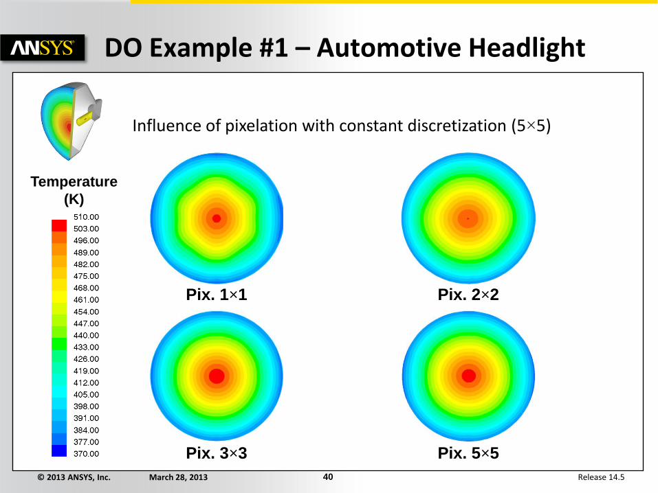
DO Example #1 – Automotive Headlight
Influence of pixelation with constant discretization (5×5)
Temperature
(K)
Pix. 1×1 Pix. 2×2
Pix. 3×3 Pix. 5×5

© 2013 ANSYS, Inc. March 28, 2013 41 Release 14.5
• DO Model allows to solve equations for a discrete number of spectral bands
• The absorption terms, the in-scattering and out-scattering terms depend on wavelength.
• Emission takes into account Planck function over the wavelength range of the band.
• For each band, 8 N N equations are solved in 3D
DO – Gray Band Model
4
0
2 ,,4
,,
dIIna
IaI
sb
s
sssr
srssr

© 2013 ANSYS, Inc. March 28, 2013 42 Release 14.5
Radiation Model
DO – Non-Gray Radiation
• Each band is defined as an interval of wavelength given for the vacuum
• You need to specify n
• Note that spectral properties of any materials are given for n = 1
• Be sure to cover the whole spectrum:
• Limit:
min
max
50000
Tn

© 2013 ANSYS, Inc. March 28, 2013 43 Release 14.5
DO – Non-Gray Radiation
• Spectral properties :
• Absorption coefficient
• Refractive index
• Boundary conditions :
• Internal emissivity and incident radiation can be specified on a band by band basis
Note: For high optical thickness (higher than 5), a second-order scheme to solve discrete ordinates is recommended
Gray-Band Absorption

© 2013 ANSYS, Inc. March 28, 2013 44 Release 14.5
DO – Advantages and Limitations
• Advantages
• Applicable to all optical thicknesses
• Particulate and anisotropic scattering (linear, Delta-Eddington, user-defined)
• Radiation in semi-transparent media (refraction, reflection)
• Diffuse and specular reflection
• Non-gray banded radiation modeling
• Various UDFs allow customization of the model and BCs
• Disadvantages
• Finite number of radiation directions causes numerical smearing
• Computationally expensive

© 2013 ANSYS, Inc. March 28, 2013 45 Release 14.5
Outline
• Radiation modelling theory
• Radiation models in FLUENT
• Surface-to-Surface (S2S)
• Discrete Ordinates (DO)
• Discrete Transfer Radiation Model (DTRM)
• P-1
• Rosseland
• Selecting a radiation model
• Postprocessing
• Conclusions
• Appendix
© 2013 ANSYS, Inc. March 28, 2013 46 Release 14.5
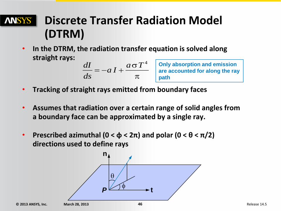
Discrete Transfer Radiation Model (DTRM)
• In the DTRM, the radiation transfer equation is solved along straight rays:
• Tracking of straight rays emitted from boundary faces
• Assumes that radiation over a certain range of solid angles from a boundary face can be approximated by a single ray.
• Prescribed azimuthal (0 < φ < 2π) and polar (0 < θ < π/2) directions used to define rays
n
t P
4TaIa
ds
dI Only absorption and emission
are accounted for along the ray
path

© 2013 ANSYS, Inc. March 28, 2013 47 Release 14.5
Radiation Model
Select File
Radiation Model
Initial calculation of ray coefficients
are saved in a .ray file
Activating the DTRM
Define Radiation… Models

© 2013 ANSYS, Inc. March 28, 2013 48 Release 14.5
DTRM – Advantages and Limitations
• Advantages
• Simple directional model (shadow effects are possible)
• Limitations
• Cannot account for scattering
• No particle/radiation interaction (too complex!)
• Computationally expensive as the number of rays increases. This can be reduced by surface and volume clustering at the expense of accuracy.
• Can only account for diffuse surfaces (not “specular” polished walls).
• Gray gas approximation (no wavelength effects)
• Cannot use hanging node adaption
• Not available in parallel
• Not conservative (difficult to verify heat balance)
• Best with optically thin media

© 2013 ANSYS, Inc. March 28, 2013 49 Release 14.5
Outline
• Radiation modelling theory
• Radiation models in FLUENT
• Surface-to-Surface (S2S)
• Discrete Ordinates (DO)
• Discrete Transfer Radiation Model (DTRM)
• P-1
• Rosseland
• Selecting a radiation model
• Postprocessing
• Conclusions
• Appendix

© 2013 ANSYS, Inc. March 28, 2013 50 Release 14.5
P-1 Model
• The P-1 model implementation in FLUENT is a four-term truncation of the general P-n model, which expands the RTE into an orthogonal series of spherical harmonics.
• Solves a simple diffusion equation for the incident radiation (G). This value is the sum of all radiative intensity in all directions.
Diffusion Emission Absorption
GaTax
G
x ii
44

© 2013 ANSYS, Inc. March 28, 2013 51 Release 14.5
P-1 Model
• Scattering effects can be modeled by altering the diffusivity:
• C is the linear-anisotropic phase function coefficient (-1 < C < 1), which dictates the fraction of radiant energy scattered forward (positive C) or backward (negative C) to the direction of incident radiation.
• Radiation flux, qi, is then
ss Ca
3
1
i
ix
Gq

© 2013 ANSYS, Inc. March 28, 2013 52 Release 14.5
P-1 Model
• Advantages
• Simple, single diffusion equation
• Computationally cheap
• Accurate for α L > 1 (coal fire)
• Allows particulate (and anisotropic) scattering
• Conservative
• Allows for the modelling of non-gray radiation using a gray-band model
• Disadvantages
• Participating media must be optically thick (α L > 1)
• Since α ~ 1 m-1 for hydrocarbon combustion, use for combustor dimensions larger than 1 meter.
• Loses accuracy at localized heat sources/sinks (tends to overpredict the radiative heat flux)
• Assumes gray gases.
• Can only account for diffuse wall surfaces (does not allow specular reflection)
© 2013 ANSYS, Inc. March 28, 2013 53 Release 14.5
Outline
• Radiation modelling theory
• Radiation models in FLUENT
• Surface-to-Surface (S2S)
• Discrete Ordinates (DO)
• Discrete Transfer Radiation Model (DTRM)
• P-1
• Rosseland
• Selecting a radiation model
• Postprocessing
• Conclusions
• Appendix

© 2013 ANSYS, Inc. March 28, 2013 54 Release 14.5
The Rosseland Model
• The other extreme is a very optically thick medium, (α L > 5)
• Radiative equilibrium is achieved and radiation acts purely diffusively with source terms due to emission.
• Radiation intensity is the black body intensity at the gas temperature
• The radiative heat flux diffuses due to high optical thickness
• Combining these equations gives a simple equation for the local radiative heat flux related to local temperature
• Example of an optically thick medium is melted glass
424 TnG
i
rx
Gq
i
rx
TTnq
3216

© 2013 ANSYS, Inc. March 28, 2013 55 Release 14.5
The Rosseland Model
• Advantages
• Computationally inexpensive
• No transport equations!
• Disadvantages
• Only valid for media with very large optical thickness
• Not available in the density-based solvers

© 2013 ANSYS, Inc. March 28, 2013 56 Release 14.5
Outline
• Radiation modelling theory
• Radiation models in FLUENT
• Surface-to-Surface (S2S)
• Discrete Ordinates (DO)
• Discrete Transfer Radiation Model (DTRM)
• P-1
• Rosseland
• Selecting a radiation model
• Postprocessing
• Conclusions
• Appendix

© 2013 ANSYS, Inc. March 28, 2013 57 Release 14.5
The Concept of Optical Thickness
• An important dimensionless number in radiation problems the optical thickness.
• Optical thickness indicates how strongly radiation is absorbed (and scattered)
• Should be used in determining which model(s) are appropriate for a given case.
• A simple measure of optical thickness is (α L)
• α = absorption coefficient (m-1)
• L = mean beam length (m) (typical distance between two opposing walls)
Optical thickness (α + σs) L α = absorption coefficient
s= scattering coefficient (often = 0)
L = mean beam length

© 2013 ANSYS, Inc. March 28, 2013 58 Release 14.5
Choosing a Radiation Model
Available Model Optical
Thickness
Surface to surface model (S2S) 0
Rosseland > 3
P-1 > 1
Discrete ordinates method (DOM) All
Discrete Transfer Radiation Model (DTRM) All
Note: S2S and DOM are the most commonly-used models

© 2013 ANSYS, Inc. March 28, 2013 59 Release 14.5
Which Model is Best for My Application?
Application Model/Method
Underhood S2S, DO
Headlamp DO (non-gray)
Combustion in large boilers DO, P1 (WSGGM)
Combustion DO, DTRM (WSGGM)
Glass applications Rosseland, P1, DO (non-gray)
Greenhouse effect DO
UV Disinfection (water treatment) DO, P1 (UDF)
HVAC DO, S2S

© 2013 ANSYS, Inc. March 28, 2013 60 Release 14.5
Selecting a Radiation Model
Discretization Memory
2×2 1.0
3×3 1.25
5×5 2.06
7×7 3.27
10×10 5.80
• Optical thickness is the key parameter but some other parameters should also be considered
• Model compatibility
• Adaption impossible when using S2S and DTRM
• DTRM is not available in parallel.
• Time for view factor calculations (S2S only)
• Memory (DO model)
≈ 1.8 kB/cell
© 2013 ANSYS, Inc. March 28, 2013 61 Release 14.5
Outline
• Radiation modelling theory
• Radiation models in FLUENT
• Surface-to-Surface (S2S)
• Discrete Ordinates (DO)
• Discrete Transfer Radiation Model (DTRM)
• P-1
• Rosseland
• Selecting a radiation model
• Postprocessing
• Conclusions
• Appendix

© 2013 ANSYS, Inc. March 28, 2013 62 Release 14.5
Postprocessing
• Radiation contours
• Incident radiation
• Radiation temperature
• Absorption coefficient
• Wall flux contours
• Radiation Heat Flux
• Surface Incident Radiation (P1,DO)
• Transmitted Radiation (for each band) (DO)
• Reflected Radiation (for each band) (DO)
• Absorbed Radiation (for each band) (DO)
• With the TUI command
solve/set/expert/keep-temporary-memory-from-being-freed? Yes
one can have access at each radiant intensity for each discrete direction (only available with DO model)

© 2013 ANSYS, Inc. March 28, 2013 63 Release 14.5
Heat Balance: Report→Fluxes
• Total Heat Transfer Rate: convective and radiative flux are taken into account
• Net heat balance should be 0 once converged or opposite to all the energy sources (UDF or constant sources, DPM)
• Radiation Heat Transfer Rate: Only radiative net flux is taken into account;
• The sum of this flux is generally different from 0. It can represent the amount of energy that is absorbed by the media.

© 2013 ANSYS, Inc. March 28, 2013 64 Release 14.5
Outline
• Radiation modelling theory
• Radiation models in FLUENT
• Surface-to-Surface (S2S)
• Discrete Ordinates (DO)
• Discrete Transfer Radiation Model (DTRM)
• P-1
• Rosseland
• Selecting a radiation model
• Postprocessing
• Conclusions
• Appendix
© 2013 ANSYS, Inc. March 28, 2013 65 Release 14.5
Conclusions
• Radiation can be expensive!
• Check order of magnitude of radiative flux compared to convective flux.
• Choose the most appropriate method to solve your problem.
• Choose resolution parameters that fits with your computers.

© 2013 ANSYS, Inc. March 28, 2013 66 Release 14.5
References
• S. Braun – UGM2003 Fluent Deutschland: “Radiation calculation in practice”
• H. Ghazialam- UGM2002 US: “Underhood flow and thermal analysis”
• FLUENT 14.5 user‘s guide
• R. Siegel & J. Howel, Thermal radiation heat transfer 4th edition
• F. P. Incropera & D. P. DeWitt, Mass Fundamental of Heat and Transfer 4th edition