HEAT TRANSFER LABORATORY

LAB MANUAL

Year : 2019 - 2020

Subject Code : AME112

Regulations : R16

Class : III B .Tech II Semester

Branch : ME

Prepared By

Dr. K. CH APPARAO, Associate Professor

Dr. CH SANDEEP, Associate Professor

MECHANICAL ENGINEERING

INSTITUTE OF AERONAUTICAL ENGINEERING (Autonomous)

Dundigal, Hyderabad - 500 043

INSTITUTE OF AERONAUTICAL ENGINEERING (Autonomous)

Dundigal, Hyderabad - 500 043

Program Outcomes

PO1 Engineering Knowledge Capability to apply the knowledge of mathematics, science and

engineering in the field of mechanical engineering.

PO2 Problem Analysis: An ability to analyze complex engineering problems to arrive at relevant

conclusion using knowledge of mathematics, science and engineering.

PO3 Design/development of solutions: Competence to design a system, component or process to

meet societal needs within realistic constraints.

PO4 Conduct investigations of complex problems: To design and conduct research oriented experiments as well as to analyze and implement data using research methodologies.

PO5 Modern tool usage: Create, select, and apply appropriate techniques, resources, and modern

engineering and IT tools including prediction and modeling to complex engineering activities

with an understanding of the limitations.

PO6 The engineer and society: Apply reasoning informed by the contextual knowledge to assess

societal, health, safety, legal and cultural issues and the consequent responsibilities relevant to

the professional engineering practice.

PO7 Environment and sustainability: Understand the impact of the professional engineering

solutions in societal and environmental contexts, and demonstrate the knowledge of, and need

for sustainable development.

PO8 Ethics: Apply ethical principles and commit to professional ethics and responsibilities and

norms of the engineering practice.

PO9 Individual and team work: Function effectively as an individual, and as a member or leader in

diverse teams, and in multidisciplinary settings.

PO10 Communication: Communicate effectively on complex engineering activities with the

engineering community and with society at large, such as, being able to comprehend and write

effective reports and design documentation, make effective presentations, and give and

receive clear instructions.

PO11 Project management and finance: Demonstrate knowledge and understanding of the

engineering and management principles and apply these to one’s own work, as a member and

leader in a team, to manage projects and in multidisciplinary environments.

PO12 Life-long learning: Recognize the need for, and have the preparation and ability to engage in

independent and life-long learning in the broadest context of technological change.

Program Specific Outcomes

PSO1 Professional Skills: To produce engineering professional capable of synthesizing and analyzing

mechanical systems including allied engineering streams.

PSO2

Problem solving skills: An ability to adopt and integrate current technologies in the design and

manufacturing domain to enhance the employability.

PSO3

Successful career and Entrepreneurship: To build the nation, by imparting technological

inputs and managerial skills to become technocrats.

INSTITUTE OF AERONAUTICAL ENGINEERING (Autonomous)

Dundigal, Hyderabad - 500 043

ATTAINMENT OF PROGRAM OUTCOMES & PROGRAM SPECIFIC OUTCOMES

Exp.

No. Name of the Experiment

Program Out

comes attained

Program specific

Outcomes attained

1 Composite slab apparatus to find overall

heat transfer coefficient

PO 1, PO 2, PO 4, PO 9 PSO1

2 Heat transfer through lagged pipe

PO 1, PO 2,

PO 4, PO 9 PSO1

3 Heat transfer through concentric sphere

PO 1, PO 2,

PO 4, PO 9 PSO1

4 Thermal conductivity of given metal rod

PO 1, PO 2,

PO 4, PO 9 PSO1

5 Heat Transfer in pin fin apparatus

PO 1, PO 2, PO 4, PO 9

PSO1

6 Experiment on transient heat conduction

PO 1, PO 2,

PO 4, PO 9 PSO1

7 Heat transfer in forced convection

PO 1, PO 2,

PO 4, PO 9 PSO1

8 Heat transfer in natural convection

PO 1, PO 2,

PO 4

PSO1

9 Parallel and Counter flow heat exchangers

PO 1, PO 2, PO 4, PO 9

PSO1

10 Emissivity apparatus – Emissivity of black

and gray body

PO 1, PO 2,

PO 4, PO 9

PSO1

11 Stefan Boltzmann apparatus

PO 1, PO 2,

PO 4

PSO1

12 Critical heat flux apparatus

PO 1, PO 2,

PO 4, PO 9

PSO1

13 Study of Heat Pipe

PO 1, PO 2, PO 4

PSO1

14 Film and drop wise condensation apparatus

PO 1, PO 2,

PO 4

PSO1

INSTITUTE OF AERONAUTICAL ENGINEERING (Autonomous)

Dundigal, Hyderabad - 500 043

CCeerrttiiffiiccaattee

This is to certify that it is a bonafied record of Practical work done by

Sri/Kum. bearing t h e

Roll No. of class

Branch in the

laboratory during the Academic

year under our supervision.

Head of the Department Lecture In-Charge

External Examiner Internal Examiner

Experiment No: 1

COMPOSITE WALL APPARATUS

AIM:

To find out total thermal resistance and total thermal conductivity of composite

wall.

DESCRIPTION:

The apparatus consists of central heater sandwiched between the slabs of MS,

Asbestos and Wood, which forms composite structure. The whole structure is well

tightened make perfect contact between the slabs. A dimmer stat is provided to vary

heat input of heaters and it is measured by a digital volt meter and ammeter.

Thermocouples are embedded between interfaces of slabs. A digital temperature

indicator is provided to measure temperature at various points.

SPECIFICATION:

1. Slab assembly arranged symmetrically on both sides of the Heater.

2. Heater coil type of 250-Watt capacity.

3. Dimmer stat open type, 230V, 0-5 amp, single phase.

4. Volt meter range 0-270V

5. Ammeter range 0-20A

6. Digital temperature indicator range 0-8000 c

7. Thermocouple used: Teflon coated, Chromal - Alumal

8. Slab diameter of each =150 mm.

9. Thickness of mild steel = 10 mm. 10.Thickness of Asbestos = 6 mm.

11. Thickness of wood= 10 mm.

PROCEDURE:

1. Start the main switch.

2. By adjusting the dimmer knob give heat input to heater. (Say 60V).

3. Wait for about 20 -30 min. approximately to reach steady state.

4. Take the readings of all (8) thermocouples.

5. Tabulate the readings in observation table.

6. Make dimmer knob to “zero” position and then put main switch off.

7. Repeat the procedure for different heat input.

OBSERVATION TABLE:

SL.NO V I T1 T2 T3 T4 T5 T6 T7 T8 T9 T10 T11 T12

1

2

3

4

5

6

7

FORMULAE:

1. Heat Input

Top Side

T mild steel = (T1 +T2)/2

T Abs = (T3 +T4)/2

T Cu = (T5 +T6)/2

Bottom Side

T mild steel = (T7 +T8)/2

T Abs = (T9 +T10)/2

T Cu = (T11 +T12)/2

2. Area of Slab

A = (π xd2)/4 (Where “d” is diameter of slab= 300 mm)

3. Thermal Conductivity ( K )

(Where L is total thickness of slab)

V×IQ =

2

K = ( )heater cooler

Q L

A T T

Experiment No: 2

LAGGED PIPE

AIM

To determine thermal conductivity of different insulating materials, Overall heat

transfer coefficient of lagged pipe and thermal resistance.

APPARATUS

The apparatus consists of three concentric pipes mounted on suitable stand. The

hollow space of the innermost pipe consists of the heater. Between first two

cylinders the insulating material with which lagging is to be done is filled

compactly. Between second and third cylinders, another material used for

lagging is filled. The third cylinder is concentric to other outer cylinder. The

thermocouples are attached to the surface of cylinders appropriately to measure

the temperatures. The input to the heater is varied through a dimmerstat .

SPECIFICATIONS:

Diameter of heater rod dH = 20 mm

Diameter of heater rod with asbestos lagging dA = 40mm

Diameter of heater rod with asbestos and saw dust lagging dS=80 mm Effective

length of the cylinder l = 500mm.

PROCEDURE:

1. Switch on the unit and check if channels of temperature indicator showing

proper change temperature.

2. Switch on the heater using the regulator and keep the power input at some

particular value.

3. Allow the unit to stabilize for about 20 to 30 minutes

4. Now note down the ammeter reading, voltmeter reading, which gives the heat

input, temperatures 1,2,3 are the temperature of heater rod, 4,5,6 are the

temperatures on the asbestos layer, 7 and 8 are the temperatures on the sawdust

lagging.

5. The average temperature of each cylinder is taken for calculation.

6. The temperatures are measured by thermocouple with multipoint digital

temperature indicator.

7. The experiment may repeat for different heat inputs.

OBSERVATIONS:

Sl.

No

V

Volt

I

amps

Heater Temp(TH) Asbestos Temp(TA) Sawdust Temp(TS)

T1 T2 T3 (TH)Avg T4 T5 T6 (TA)Avg T7 T8 (TS)Avg

1

2

3

(TH)Aveg = (T1+T2+T3)/3 0C

(TA)Aveg = (T4+T5+T6)/3 0C

(TS)Aveg = (T7+T8)/2 0C

Q = VxI

Thermal conductivity of lagged pipe

PRECAUTIONS:

1) Keep dimmer stat to ZERO position before start.

2) Increase voltage gradually.

3) Keep the assembly undisturbed while testing.

4) While removing or changing the lagging materials do not

disturb the thermocouples.

5) Do not increase voltage above 150V

6) Operate selector switch of temperate indicator gently.

RESULTS: Thermal conductivity of different insulating materials, Overall heat

transfer coefficient of lagged pipe and thermal resistance has been determined.

1. Thermal conductivity of asbestos powder lagging kAsbestos =…………………

2. Thermal conductivity of sawdust lagging kSawdust =……………………….

3. Overall heat transfer coefficient U=…………………………

4. Thermal resistance of Asbestos RAsbestos =……………………………

5. Thermal resistance of Sawdust RSawdust =………………………………..

0

i

i o

rQ × ln

rK =

2 π L (T - T )

Experiment No : 3

THERMAL CONDUCTIVITY OF INSULATING POWDER

AIM:

To determine the thermal conductivity of insulating powder at various heat

inputs.

THEORY:

FORIER LAW OF HEAT CONDUCTION:

A Materials having lower thermal conductivity are called insulators.

Examples for good conductors include all metals. While asbestos, magnesia, glass

wool etc., are some the examples for insulators.

The radial heat conduction for single hollow sphere transferring heat from inside to

outside is given by

This law states that rate of heat flow through a surface is directly

proportional to the area normal to the surface and the temperature gradient across

the surface.

Negative sign indicates that the heat flows from higher temperature to the lower

temperature. K is called the thermal conductivity.

THERMAL CONDUCTIVITY:

This can be defined as the amount of heat that can flow per unit time across a unit

0 i i o

o i

4 π K r r (T - T )Q =

(r - r )

dTQ = - K A

dx

cross sectional area when the temperature gradient is unity. The units of thermal

conductivity are w/m-K. Materials having higher thermal conductivity are called

conductors while those

Where:

Q = rate of heat transfer in watts = V X I

k = Thermal conductivity w/m-k

ri = radius of inner sphere in meters

ro = radius of outer sphere in meters

Ti =Temperature of the inner sphere

To =Temperature of the outer sphere

DESCRIPTION OF APPARATUS:

The apparatus consists of two concentric copper spheres. Heating coils is provided

in the inner sphere. The space between the inner and outer spheres are filled by the

insulating powder whose thermal conductivity is to be determined. The power

supply to the heating coils is adjusted by using dimmer stat. Chromel - Alumel

thermocouples are used to record the temperatures. Thermocouples 1 to 6 are

embedded on the surface of inner sphere and 7 to 12 are embedded on the outer

SPECIFICATIONS:

1. Radius of inner sphere = 50mm

2. Radius of outer sphere = 100 mm

3. Voltmeter 0-300V & Ammeter 0-5amps.

4. Dimmer stat – 2 amps.

5. Temperature indicator 0-3000c

PROCEDURE:

1. Connect the unit to an AC source 240 V 5amps and switch on the MCB.

2. Operate the dimmer stat slowly to increase the heat input to the heater

and adjust the voltage to any desired voltage (do not exceed 150V).

3. Maintain the same heat input throughout the experiment until the

temperature reaches a steady state.

4. Note down the following readings provided in the Observation table.

5. Repeat the experiment for other heat inputs.

Sl.

No.

Heat Input Inner Surface temp C Outer Surface temp C

V A T1 T2 T3 T4 T5 T6 T7 T8 T9 T10 T11 T12

1.

2.

3.

PRECAUTIONS:

4. Keep the dimmer stat to zero before starting the experiment.

5. Take readings at study state condition only.

6. Use the selector switch knob and dimmer knob gently.

RESULT:

The thermal conductivity of insulating powder at various heat inputs has been

determined.

1 2 3 4 5 6i

T + T + T + T + T + TAverage T =

6

7 8 9 10 11 120

T + T + T + T + T + TAverage T =

6

0 i

i o i o

Q ( r - r )K =

4 π r r (T - T )

Experiment N0 : 4

THERMAL CONDUCTIVITY OF METAL ROD

AIM:

To determine the thermal conductivity of given metal rod.

THEORY:

From Fourier’s law of heat conduction

Q = Rate of heat conducted, W

A = Area of heat transfer, m²

k = Thermal conductivity of the material, W/m-K

dT/dx = Temperature gradient

Thermal conductivity is a property of the material and may be defined as the

amount of heat conducted per unit time through unit area, when a temperature

difference of unit degree is maintained across unit thickness.

DESCRIPTION OF THE APPARATUS:

The apparatus consists of a brass rod, one end of which is heated by an electric

heating coil while the other end projects into the cooling water jacket. The rod is

insulated with glass wool to minimize the radiation and convection loss from the

surface of the rod and thus ensure nearly constant temperature gradient throughout

the length of the rod. The temperature of the rod is measured at five different

locations. The heater is provided with a dimmerstat for controlling the heat input.

Water is circulated through the jacket and its flow rate and temperature rise can be

measured.

dTQ = - K A

dx

SPECIFICATIONS :

Specimen material : Brass rod

Size of the Specimen : ϕ20 mm, 450mm long

Cylindrical shell : 300mm long

Voltmeter : Digital type, 0-300volt, AC

Ammeter : Digital type, 0-20amp,

AC Dimmer for heating Coil : 0-230v, 12amps

Heater : Band type Nichrome heater, 250 W

Thermocouple used : 11 nos

Temperature indicator : Digital type, 0-2000c, Cr-Al

PRODEDURE:

1. Power supply is given to the apparatus.

2. Give heat input to the heater by slowly rotating the dimmer and adjust the voltage

to say 60 V, 80 V, etc

3. Start the cooling water supply through the jacket and adjust its flow rate so that the

heat is taken away from the specimen constantly.

4. Allow sufficient time for the apparatus to reach steady state.

5. Take readings of voltmeter and ammeter.

6. Note the temperatures along the length of the specimen rod at 5 different locations.

7. Note down the inlet & outlet temperatures of cooling water and measure the flow

rate of water.

8. Repeat the experiment for different heat inputs.

OBSERVATION TABLE:

‘V’

Volt

‘I’

Amp

Metal rod thermocouple reading

(0C)

Water

temp (0C) Volume

flow rate

of water,

V

cc/min

In let

Ou tlet

T1 T2 T3 T4 T5 T6 T7 T8 T9 T10 T11

1.

2.

3.

CALCULATION:

Plot the variation of temperature along the length of the rod. From the graph,

obtain dT/dx, which is the slope of the straight line passing through/near to the

points in the graph. Assuming no heat loss, heat conducted through the rod = heat

carried away by the cooling water

Ka dT/dx = mf Cp (T11 –T10)

Where, ‘k’ = thermal conductivity of metal rod, (W/m-K)

‘A’ = Cross sectional area of metal rod = πd²/4 (m²)

‘d’ = diameter of the specimen = 20 mm

‘Cp’ = Specific heat of water = 4.187 kJ/kg-K

Thus, the thermal conductivity ‘k’ of metal rod can be evaluated.

PRECAUTIONS:

7. Keep the dimmer stat to zero before starting the experiment.

8. Take readings at study state condition only.

9. Use the selector switch knob and dimmer knob gently.

RESULT:

The thermal conductivity of given metal rod has been determined.

f p 11 12m C (T - T ) K =

dTA

dx

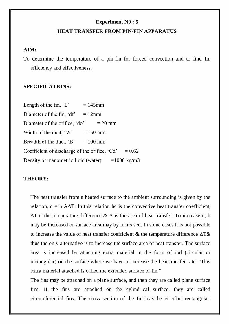
Experiment N0 : 5

HEAT TRANSFER FROM PIN-FIN APPARATUS

AIM:

To determine the temperature of a pin-fin for forced convection and to find fin

efficiency and effectiveness.

SPECIFICATIONS:

Length of the fin, ‘L’ = 145mm

Diameter of the fin, ‘df’ = 12mm

Diameter of the orifice, ‘do’ = 20 mm

Width of the duct, ‘W’ = 150 mm

Breadth of the duct, ‘B’ = 100 mm

Coefficient of discharge of the orifice, ‘Cd’ = 0.62

Density of manometric fluid (water) =1000 kg/m3

THEORY:

The heat transfer from a heated surface to the ambient surrounding is given by the

relation, q = h AΔT. In this relation hc is the convective heat transfer coefficient,

ΔT is the temperature difference & A is the area of heat transfer. To increase q, h

may be increased or surface area may by increased. In some cases it is not possible

to increase the value of heat transfer coefficient & the temperature difference ΔT&

thus the only alternative is to increase the surface area of heat transfer. The surface

area is increased by attaching extra material in the form of rod (circular or

rectangular) on the surface where we have to increase the heat transfer rate. "This

extra material attached is called the extended surface or fin."

The fins may be attached on a plane surface, and then they are called plane surface

fins. If the fins are attached on the cylindrical surface, they are called

circumferential fins. The cross section of the fin may be circular, rectangular,

triangular or parabolic.

Temperature distribution along the length of the fin:

Where

T = Temperature at any distance x

on the fin

T0 = Temperature at x = 0

T = Ambient temperature

L = Length of the fin

Where

h = convective heat transfer coefficient P = Perimeter of the fin

A = area of the fin

K = Thermal conductivity of the fin

Rate of heat flow for end insulated condition:

Effectiveness of a fin is defined as the ratio of the heat transfer with fin to the heat

transfer from the surface without fins.

The efficiency of a fin is defined as the ratio of the actual heat transferred by

the fin to the maximum heat transferred by the fin if the entire fin area were at base

temperature.

Procedure:

1. Connect the equipment to electric power supply.

2. Keep the thermocouple selector switch to zero position.

3. Turn the dimmer stat clockwise and adjust the power input to the heater to the

desired value and switch on the blower.

4. Set the air–flow rate to any desired value by adjusting the difference in water

levels in the manometer and allow the unit to stabilize.

5. Note down the temperatures, T1 to T6 from the thermocouple selector switch.

Note down the difference in level of the manometer and repeat the experiment for

different power inputs to the heater.

PRECAUTIONS:

3. Never switch on main power supply before ensuring that all on/off switches given

on the panel are at off position

4. Never run the apparatus if power supply is less than 180 or above 200 volts.

RESULT:

The temperature distribution of a pin – fin for forced convectio

Experiment No: 6

UNSTEADY STATE HEAT TRANSFER

AIM:

To obtain the specimen temperature at any interval of time by theoretical methods

and observe the heating and cooling curves of unsteady state.

INTRODUCTION:

Unsteady state designates a phenomenon which is time dependent. Conduction of

heat in unsteady state refers to transient conditions where in, heat flow and

temperature distribution at any point of system varies with time. Transient

conditions occur in heating or cooling of metal billets, cooling of IC engine

cylinder, brick and vulcanization of rubber.

DESCRIPTION:

Unsteady state heat transfer equipment has oil check which is at top of oil heater.

Thermocouple No.1is located inside the specimen No.2 thermocouple measures the

atmospheric temperature. No.3 thermocouple measures the oil temperature.

Digital temperature indicator indicates respective temperatures of thermocouples

as we select it by selector switch. Heater ON/OFF toggle switch and buzzer

ON/OFF toggle switch is provided on the control panel.

SPECIFICATIONS:

1. D.C Buzzer : 10-30 volt

2. Oil Heater : 1 kW

3. Digital temperature indicator : 1200C0

4. Thermocouple : Al-Cr type

5. Specimens material : Copper

6. Fuse : 4 Amps.

EXPERIMENTATION:

Obtain the specimen temperature at any interval of time by practical and by

theoretical methods and observe the heating and cooling curves of unsteady state.

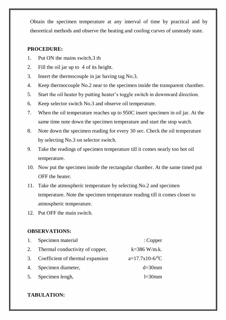
PROCEDURE:

1. Put ON the mains switch.3 th

2. Fill the oil jar up to 4 of its height.

3. Insert the thermocouple in jar having tag No.3.

4. Keep thermocouple No.2 near to the specimen inside the transparent chamber.

5. Start the oil heater by putting heater’s toggle switch in downward direction.

6. Keep selector switch No.3 and observe oil temperature.

7. When the oil temperature reaches up to 950C insert specimen in oil jar. At the

same time note down the specimen temperature and start the stop watch.

8. Note down the specimen reading for every 30 sec. Check the oil temperature

by selecting No.3 on selector switch.

9. Take the readings of specimen temperature till it comes nearly too hot oil

temperature.

10. Now put the specimen inside the rectangular chamber. At the same timed put

OFF the heater.

11. Take the atmospheric temperature by selecting No.2 and specimen

temperature. Note the specimen temperature reading till it comes closer to

atmospheric temperature.

12. Put OFF the main switch.

OBSERVATIONS:

1. Specimen material : Copper

2. Thermal conductivity of copper, k=386 W/m.k.

3. Coefficient of thermal expansion a=17.7x10-6/0C

4. Specimen diameter, d=30mm

5. Specimen lengh, l=30mm

TABULATION:

In case of Heating: In case of Cooling:

Oil Specimen Time Sl.

No

Specimen Time

in

second

t

Sl. tempera Temperatu in Atmospheric Temperatur

N ture T1 re T3 in 0C secon temperature e T3 in 0C at

o in 0C at interval d T2 in 0C interval of of 30 sec. t 30 sec

1. 70 0 1. 0

2. 30 2. 30

3. 60 3. 60

4. 90 4. 90

5. 120 5. 120

6. 150 6. 150

7. 180 7. 180

8. 240 8. 240

9. 270 9. 270

10 300 10.

300

.

11 330 11 330

CALCULATION:

Specimen material : Copper Thermal conductivity of copper,k=386 W/m0k.

Coefficient of thermal expansion a=17.7x10-6/0C

Specimen diameter, d = 30mm

Specimen length, l = 30mm

Characteristic length for cylinder L = d/2

Biot number Bi= hL/k

Fourier number Fo= αT/L2

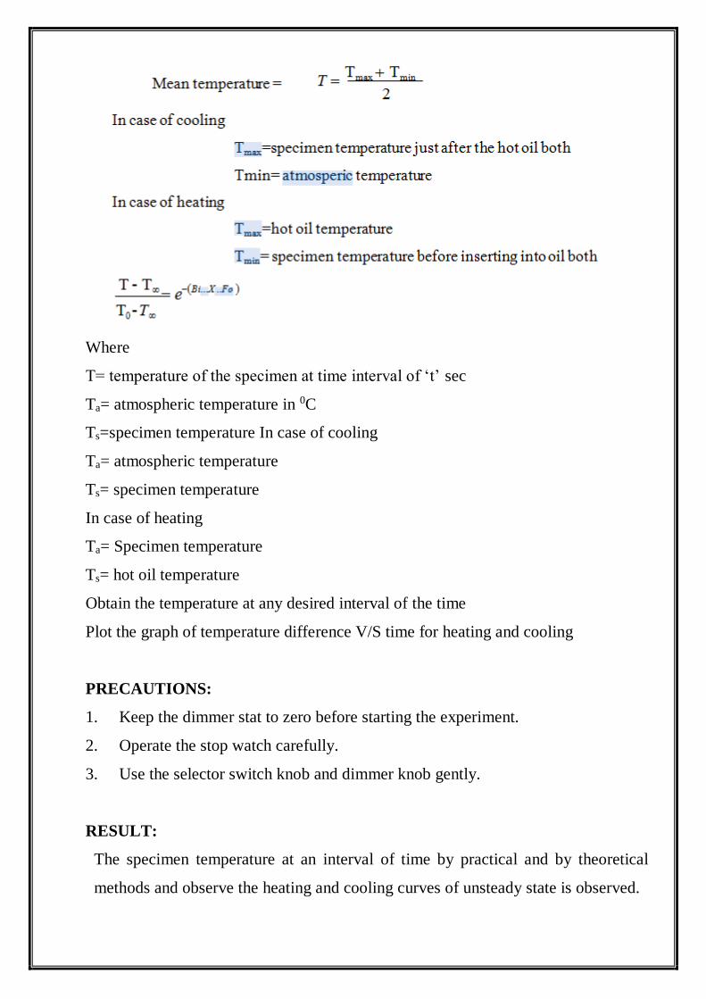
Where

T= temperature of the specimen at time interval of ‘t’ sec

Ta= atmospheric temperature in 0C

Ts=specimen temperature In case of cooling

Ta= atmospheric temperature

Ts= specimen temperature

In case of heating

Ta= Specimen temperature

Ts= hot oil temperature

Obtain the temperature at any desired interval of the time

Plot the graph of temperature difference V/S time for heating and cooling

PRECAUTIONS:

1. Keep the dimmer stat to zero before starting the experiment.

2. Operate the stop watch carefully.

3. Use the selector switch knob and dimmer knob gently.

RESULT:

The specimen temperature at an interval of time by practical and by theoretical

methods and observe the heating and cooling curves of unsteady state is observed.

Experiment No: 7

HEAT TRANSFER BY FORCED CONVECTION

AIM:

To determine the convective heat transfer coefficient and the rate of heat transfer by

forced convection for flow of air inside a horizontal pipe.

THEORY:

Convective heat transfer between a fluid and a solid surface takes place by the

movement of fluid particles relative to the surface. If the movement of fluid

particles is caused by means of external agency such as pump or blower that forces

fluid over the surface, then the process of heat transfer is called forced convection.

In convectional heat transfer, there are two flow regions namely laminar &

turbulent. The non-dimensional number called Reynolds number is used as the

criterion to determine change from laminar to turbulent flow. For smaller value of

Reynolds number viscous forces are dominant and the flow is laminar and for larger

value of Reynolds numbers the inertia forces become dominant and the flow is

turbulent. Dittus –Boelter correlation for fully developed turbulent flow in circular

pipes is,

Where

Nu = 0.023 (Re) 0.8 (Pr) n (from data book)

n = 0.4 for heating of fluid

n = 0.3 for cooling of fluid

Nusselt number= Nu = hd/k

Re = Reynolds Number = Vd/ρ

P = Prandtl Number = µCP/k

DESCRIPTION OF THE APPARATUS:

The apparatus consists of a blower to supply air. The air from the blower passes

through a flow passage, heater and then to the test section. Air flow is measured by

an orifice meter placed near the test section. A heater placed around the tube heats

the air, heat input is controlled by a dimmer stat. Temperature of the air at inlet and

at outlet are measured using thermocouples. The surface temperature of the tube

wall is measured at different sections using thermocouples embedded in the walls.

Test section is enclosed in a asbestos rope where the circulation of rope is avoid the

heat loss to outside.

PROCEDURE:

1. Start the blower after keeping the valve open, at desired rate.

2. Put on the heater and adjust the voltage to a desired value and maintain it as

constant

3. Allow the system to stabilize and reach a steady state.

4. Note down all the temperatures T1 to T7, voltmeter and ammeter readings, and

manometer readings.

5. Repeat the experiment for different heat input and flow rates.

SPECIFICATIONS:

Specimen : Copper Tube

Size of the Specimen : I.D. 25mm x 300mm long

Heater : Externally heated, Nichrome wire Band Heater

Ammeter : Digital type, 0-20amps, AC

Voltmeter : Digital type, 0-300volts, AC

Dimmer stat for heating Coil : 0-230v, 2amps

Thermocouple Used : 7 nos.

Centrifugal Blower : Single Phase 230v, 50 hz, 3000rpm

Manometer : U-tube with water as working fluid

Orifice diameter, ‘d2’ : 20 mm

G. I pipe diameter, ‘d1’ : 40 mm

Coefficient of discharge : 0.62

Length of the tube : 500 mm

OBSERVATION TABLE:

Sl.

No

Heater input Q

(Watts)

Diff. in

Mano

meter

reading

hm mm

Air temp. °C Tube surface Temperature °C

V

volt

I

amp

V X I Inlet

T1

Outlet

T7

T2

T3

T4

T5

T6

1.

2.

3.

a1 is area of GI pipe (diameter = 40mm)

a2 is area of orifice (diameter = 20mm)

Properties of air are taken at temperature Tf = (Th +Ts)/2

Th is average surface temperature of the tube

Th = (T2+T3+T4+T5)/4

Mean Temperature of Ts = (T1+T6)/2

PRECAUTIONS:

1. Never switch on main power supply before ensuring that all on/off switches

given on the panel are at off position

2. Never run the apparatus if power supply is less than 180 or above 200 volts.

RESULT:

The convective heat transfer coefficient and the rate of heat transfer by forced

convection for flow of air inside a horizontal pipe has been determined.

1. The convective heat transfer coefficient by forced convection h=………………

2. The rate of heat transfer by forced convection Q=………………………………..

Experiment No: 8

HEAT TRANSFER BY NATURAL CONVECTION

AIM:

To find out heat transfer coefficient and heat transfer rate from vertical cylinder in

natural convection.

THEORY:

Natural convection heat transfer takes place by movement of fluid particles on

solid surface caused by density difference between the fluid particles on account of

difference in temperature. Hence there is no external agency facing fluid over the

surface. It has been observed that the fluid adjacent to the surface gets heated,

resulting in thermal expansion of the fluid and reduction in its density.

Subsequently a buoyancy force acts on the fluid causing it to flow up the surface.

Here the flow velocity is developed due to difference in temperature between fluid

particles.

The following empirical correlations may be used to find out the heat transfer

coefficient for vertical cylinder in natural convection.

β = Coefficient of Volumetric expansion (or) temperature co-efficient of thermal

conductivity in 1/K

SPECIFICATIONS:

Specimen : Stainless Steel tube,

Size of the Specimen : Outer diameter 45mm, 500mm length

Heater : Nichrome wire type heater along its length

Thermocouples used : 6nos.

Ammeter : Digital type, 0-2amps, AC

Voltmeter : Digital type, 0-300volts,

AC Dimmer stat for heating coil : 0-230 V, 2 amps, AC power

Enclosure with acrylic door: For visual display of test section (fixed)

APPARATUS:

The apparatus consists of a stainless steel tube fitted in a rectangular duct in a

vertical position. The duct is open at the top and bottom and forms an enclosure

and serves the purpose of undisturbed surroundings. One side of the duct is made

of acrylic sheet for visualization. A heating element is kept in the vertical tube,

which heats the tube surface. The heat is lost from the tube to the surrounding air

by natural convection. Digital temperature indicator measures the temperature at

different points with the help of seven temperature sensors, including one for

measuring surrounding temperature. The heat input to the heater is measured by

Digital Ammeter and Digital Voltmeter and can be varied by a dimmer stat.

PROCEDURE:

1. Ensure that all ON/OFF switches given on the panel are at OFF position.

2. Ensure that variac knob is at zero position, provided on the panel.

3. Now switch on the main power supply (220 V AC, 50 Hz).

4. Switch on the panel with the help of mains ON/OFF switch given on the panel.

5. Fix the power input to the heater with the help of variac, voltmeter and ammeter

provided.

6. Take thermocouple, voltmeter & ammeter readings when steady state is reached.

7. When experiment is over, switch off heater first.

8. Adjust variac to zero position.

9. Switch off the panel with the help of Mains On/Off switch given on the panel.

10. Switch off power supply to panel.

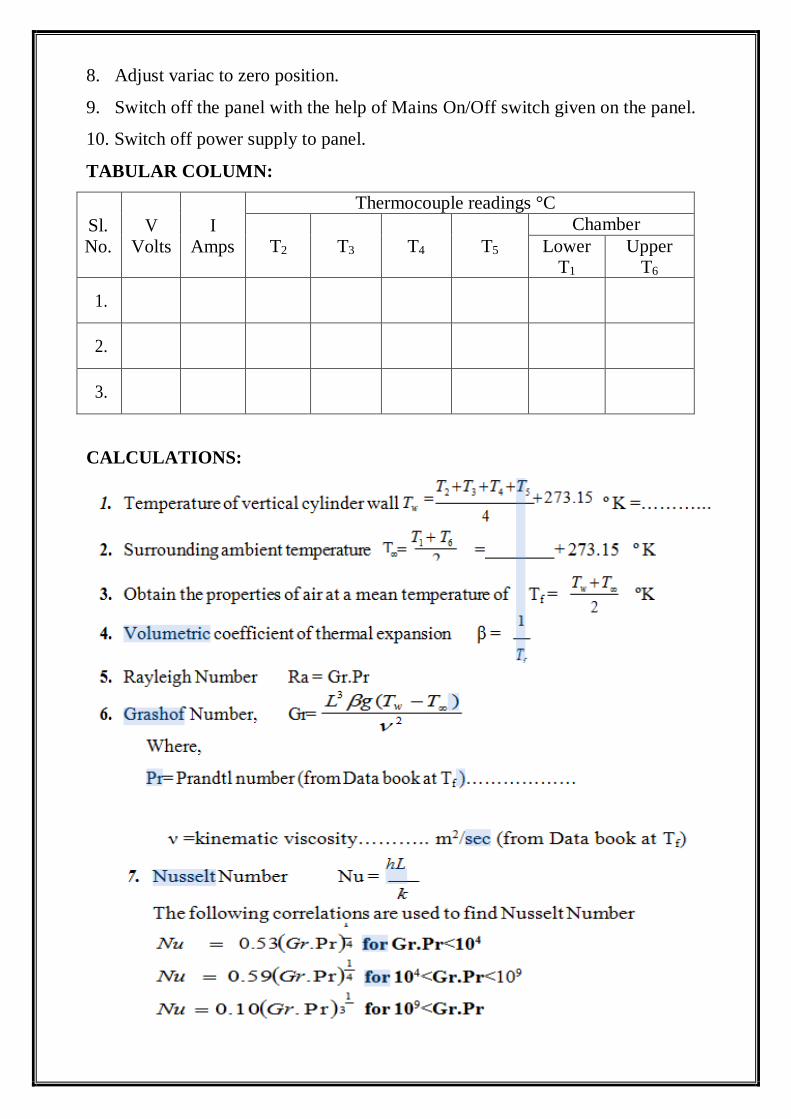
TABULAR COLUMN:

Sl.

No.

V

Volts

I

Amps

Thermocouple readings °C

T2

T3

T4

T5

Chamber

Lower T1

Upper T6

1.

2.

3.

CALCULATIONS:

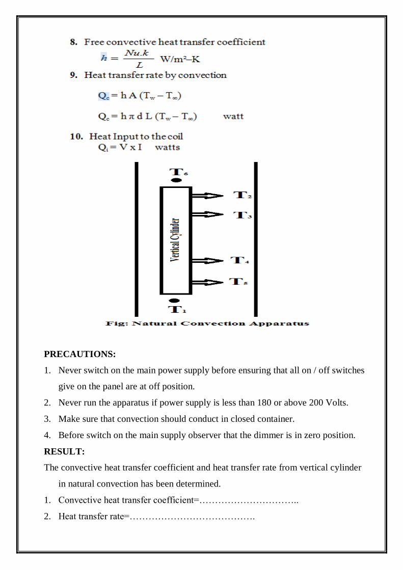
PRECAUTIONS:

1. Never switch on the main power supply before ensuring that all on / off switches

give on the panel are at off position.

2. Never run the apparatus if power supply is less than 180 or above 200 Volts.

3. Make sure that convection should conduct in closed container.

4. Before switch on the main supply observer that the dimmer is in zero position.

RESULT:

The convective heat transfer coefficient and heat transfer rate from vertical cylinder

in natural convection has been determined.

1. Convective heat transfer coefficient=…………………………..

2. Heat transfer rate=………………………………….

Experiment No: 9

PARALLEL FLOW AND COUNTER FLOW HEAT EXCHANGER

AIM:

To determine LMTD, effectiveness and overall heat transfer coefficient for parallel

and counter flow heat exchanger

SPECIFICATIONS:

Length of heat exchanger L = 2440 MM

Inner copper tube ID = 12 mm

OD = 15 mm

Outer GI tube ID = 40 mm

Geyser capacity =1 Lt, 3 kW

THEORY:

Heat exchanger is a device in which heat is transferred from one fluid to another.

Common examples of heat exchangers are:

i. Condensers and boilers in steam plant

ii. Inter coolers and pre-heaters

iii. Automobile radiators

iv. Regenerators

CLASSIFICATION OF HEAT EXCHANGERS:

1. Based on the nature of heat exchange process:

i. Direct contact type – Here the heat transfer takes place by direct mixing of

hot and cold fluids

ii. Indirect contact heat exchangers – Here the two fluids are separated

through a metallic wall. ex. Regenerators, Recuperators etc

2. Based on the relative direction of fluid flow:

i. Parallel flow heat exchanger – Here both hot and cold fluids flow in the

same direction.

ii. Counter flow heat exchanger – Here hot and cold fluids flow in opposite

direction.

iii. Cross-flow heat exchangers – Here the two fluids cross one another.

CLASSIFICATION OF HEAT EXCHANGERS:

1. Based on the nature of heat exchange process:

i. Direct contact type – Here the heat transfer takes place by direct mixing of

hot and cold fluids

ii. Indirect contact heat exchangers – Here the two fluids are separated

through a metallic wall. ex. Regenerators, Recuperators etc

2. Based on the relative direction of fluid flow:

i. Parallel flow heat exchanger – Here both hot and cold fluids flow in the

same direction.

ii. Counter flow heat exchanger – Here hot and cold fluids flow in opposite

direction.

iii. Cross-flow heat exchangers – Here the two fluids cross one another.

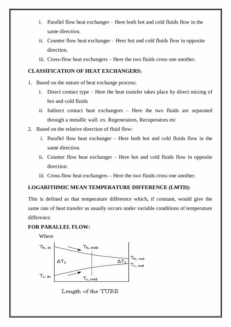
LOGARITHMIC MEAN TEMPERATURE DIFFERENCE (LMTD):

This is defined as that temperature difference which, if constant, would give the

same rate of heat transfer as usually occurs under variable conditions of temperature

difference.

FOR PARALLEL FLOW:

Where

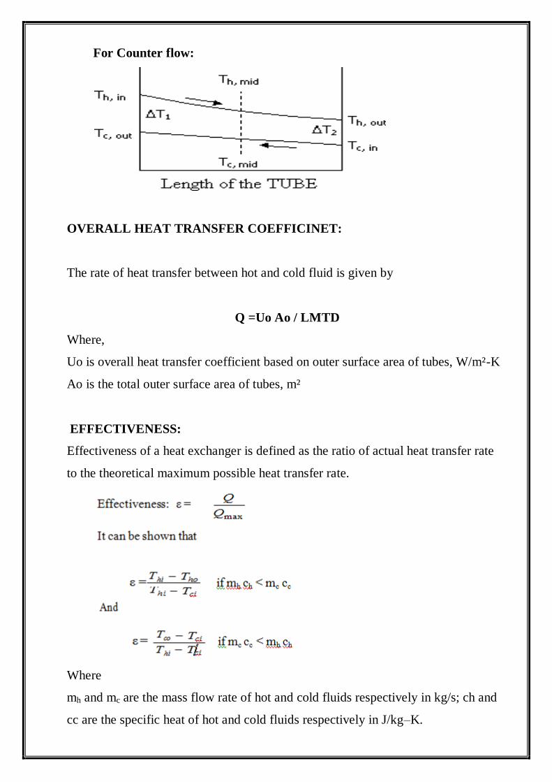
For Counter flow:

OVERALL HEAT TRANSFER COEFFICINET:

The rate of heat transfer between hot and cold fluid is given by

Q =Uo Ao / LMTD

Where,

Uo is overall heat transfer coefficient based on outer surface area of tubes, W/m²-K

Ao is the total outer surface area of tubes, m²

EFFECTIVENESS:

Effectiveness of a heat exchanger is defined as the ratio of actual heat transfer rate

to the theoretical maximum possible heat transfer rate.

Where

mh and mc are the mass flow rate of hot and cold fluids respectively in kg/s; ch and

cc are the specific heat of hot and cold fluids respectively in J/kg–K.

DESCRIPTION OF THE APPRATUS:

The apparatus consists of a concentric tube heat exchanger. The hot fluid namely

hot water is obtained from the Geyser (heater capacity 3 kW) & it flows through

the inner tube. The cold fluid i.e. cold water can be admitted at any one of the ends

enabling the heat exchanger to run as a parallel flow or as a counter flow

exchanger. Measuring jar used for measure flow rate of cold and hot water. This

can be adjusted by operating the different valves provided. Temperature of the

fluid can be measured using thermocouples with digital display indicator. The

outer tube is provided with insulation to minimize the heat loss to the

surroundings.

PROCEDURE:

1. First switch ON the unit panel

2. Start the flow of cold water through the annulus and run the exchanger as

counter flow or parallel flow.

3. Switch ON the geyser provided on the panel & allow to flow through the inner

tube by regulating the valve.

4. Adjust the flow rate of hot water and cold water by using rotameters & valves.

5. Keep the flow rate same till steady state conditions are reached.

6. Note down the temperatures on hot and cold water sides. Also note the flow

rate.

7. Repeat the experiment for different flow rates and for different temperatures.

The same method is followed for parallel flow also.

OBSERVATION TABLE: (Parallel Flow)

Sl. No.

Hot water

flow rate

mh, kg/s

Cold water

flow rate

mc, kg/s

Temperature of cold water in °C

Temp. of hot water in °C

Inlet Tci

Outlet Tco

Inlet Thi

Outlet Tho

1.

2.

3.

Counter Flow

Sl. No.

Hot water

flow rate

mh, kg/s

Cold water

flow rate

mc, kg/s

Temperature of

cold water in °C

Temp. of hot

water in °C

Inlet Tci

Outlet Tco

Inlet Thi

Outlet Tho

1.

2.

3.

1. Heat transfer from hot water Qh = mh Cph (Thi –Tho)watts

mh = mass flow rate of hot water kg/sec

Cph = Specific heat of hot water = 4186.8 J kg-K

2. Heat gain by the cold fluid

Qc = mc Cpc (Tco- Tci) watts

mc = Mass flow of cold fluid, kg/s

Cpc = Specific heat of cold fluid = 4186.8 J/kg –K

LMTD = (θ1 – θ2)/ln(θ1/θ2)

θ1 = Thi – Tci and

θ2 = Tho – Tco for parallel flow heat exchanger

θ1 = Tho – Tci and

θ2 = Thi – Tco for counter flow heat exchanger

5.Overall heat transfer coefficient based on outside surface area of inner tube

0

0

QU =

A .LMTD

Where,

Ao =π do L m²

do = Outer diameter of the tube = 0.0125 m

L = length of the tube = 1.5 m

RESULT:

The overall heat transfer coefficient of parallel flow and counter flow heat

exchangers has been determined.

Experiment No: 10

EMISSIVITY MEASUREMENT OF RADIATING SURFACES

AIM:

To determine the emissivity of given test plate surface.

THEORY:

Any hot body maintained by a constant heat source, loses heat to surroundings by

conduction, convection and radiation. If two bodies made of same geometry are

heated under identical conditions, the heat loss by conduction and convection can be

assumed same for both the bodies, when the difference in temperatures between

these two bodies is not high. In such a case, when one body is black & the other

body is gray from the values of different surface temperatures of the two bodies

maintained by a constant power source emissivity can be calculated. The heat loss

by radiation depends on

a) Characteristic of the material

b) Geometry of the surface and

c) Temperature of the surface

The heat loss by radiation when one body is completely enclosed by the other

body is given by

If a body is losing heat to the surrounding atmosphere, then the area of atmosphere

A2 >> area of body A1. Thus if anybody is losing heat by radiation to the

surrounding atmosphere equation (1) takes the form.

Q = σ ε A (T1 4 -T2

4 )

4 4

1 1 2

1

1 2 2

A (T - T ) Q =

A1 1+ 1

A

Where

σ = Stefan Boltzmannn constant = 5.6697 x 10-8 W/m² K4

A1 = Surface area in m²

ε = Emissivity

T1 = surface temperature of the body in K and

T2 = surrounding atmospheric temperature in K

Let us consider a black body & a gray body with identical geometry being heated

under identical conditions, assuming conduction & convection heat loss to remain

the same.

Let Qb and Qg be the heat supplied to black & gray bodies respectively. If heat input to

both the bodies are same,

Qb = Qg

Assuming, heat loss by conduction and convection from both bodies to remain

same.

Heat loss by radiation by the black body = Heat loss by radiation by the gray body

Where

Suffix ‘b’ stands for black body,

Suffix ‘g’ stands for gray body,

Suffix ‘c’ stands for chamber.

DESCRIPTION:

The experimental set up consists of two circular aluminium plates of identical

dimensions. One of the plates is made black by applying a thick layer of lamp black

while the other plate whose emissivity is to be measured is a gray body. Heating

Heat loss by radiation by the black body = Heat loss by radiation by the gray body

4 4 4 4Q = A (T - T ) A (T - T ) b b b a g g g a

coils are provided at the bottom of the plates. The plates are mounted on asbestos

cement sheet and kept in an enclosure to provide undisturbed natural convection

condition. Three thermocouples are mounted on each plate to measure the average

temperature. One thermocouple is in the chamber to measure the ambient

temperature or chamber air temperature. The heat input can be varied with

the help of variac for both the plates , that can be measured using digital volt and

ammeter.

SPECIFICATIONS:

Specimen material : Aluminum

Specimen Size : ϕ 150 mm, 10 mm thickness (gray & black body)

Voltmeter : Digital type, 0-300v

Ammeter : Digital type, 0-3 amps

Dimmer stat : 0-240 V, 2 amps

Temperature Indicator : Digital type, 0-300°C,

K type Thermocouple Used : 7 nos.

Heater : Sand witched type Nichrome heater, 400 W

PROCEDURE:

1. Switch on the electric mains.

2. Operate the dimmer stat very slowly and give same power input to both the

heater Say 60 V by using (or) operating cam switches provided panel.

3. When steady state is reached note down the temperatures T1 to T7 by rotating the

temperature selection switch gently.

4. Also note down the volt & ammeter reading

5. Repeat the experiment for different heat inputs.

OBSERVATION TABLE:

Sl.

No.

Heater input

Temperature of black

surface °C

Temperature of gray

surface °C

Chamber

Temp °C

V I T1 T2 T3 T5 T6 T7 T4

1.

2.

3.

SPECIMEN CALCULATIONS:

Experiment No: 11

STEFAN BOLTZMANN APPARATUS

AIM:

To determine the value of Stefan Boltzmann constant for radiation heat transfer.

APPARATUS:

Hemisphere, Heater, Temperature indicator, Stopwatch.

THEORY:

Stefan Boltzmann law states that the total emissive power of a perfect black body is

proportional to fourth power of the absolute temperature of black body surface.

Eb = σT4

Where

σ = Stefan Boltzmann constant = 5.6697 x 10-8 W/(m² K4)

DESCRIPTION:

The apparatus consists of a flanged copper hemisphere fixed on a flat non-

conducting plate. A test disc made of copper is fixed to the plate. Thus the test disc

is completely enclosed by the hemisphere. The outer surface of the hemisphere is

enclosed in a vertical water jacket used to heat the hemisphere to a suitable

constant temperature. Three Cr-Al thermocouples are attached at three strategic

places on the surface of the hemisphere to obtain the temperatures. The disc is

mounted on an ebonite rod which is fitted in a hole drilled at the center of the base

plate. Another Cr-Al thermocouple is fixed to the disc to record its temperature.

Fill the water in the SS water container with immersion heater kept on top of the

panel.

SPECIFICATIONS:

Specimen material : Copper

Size of the disc : ϕ 20mm x 0.5mm thickness

Base Plate : ϕ250mm x 12mm thickness (hylam)

Heater :1.5 kW capacity, immersion type

Copper Bowl : ϕ 200mm

Digital temperature indicator :0 -199.9° C

Thermocouples used :3 nos. on hemisphere

Stop Watch :Digital type

Overhead Tank :SS, approx. 12 liter capacity

Water Jacket :ϕ 230 mm, SS

Mass of specimen, ‘m’ :5 gm Specific heat of the disc

Cp :0.38 kJ/kg K

PROCEDURE:

1. Remove the test disc before starting the experiment.

2. Allow water to flow through the hemisphere, Switch on the heater and allow

the hemisphere to reach a steady state temperature.

3. Note down the temperatures T1,T2 & T3. The average of these temperatures is

the hemisphere temperature Th .

4. Insert the test disc at the bottom of the hemisphere and lock it. Start the stop

clock simultaneously.

5. Note down the temperature of the test disc at an interval of about 15 sec for

about 15 to 20 minutes.

OBSERVATION TABLE:

Let Td = Temperature of the disc before inserting into the plate in K

Thermocouple

Temperature of the

copper hemisphere °

C

T1

T2

T3

Th Average of T1 , T2 and T3 =

Temperature – time response of test disc:

Time ‘t’

sec

Temper

ature Td

° C

Time

‘t’

sec

Temper

ature Td

° C

CALCULATIONS:

1. Plot the graph of temperature of the disc v/s time to obtain the slope (dT/dt) of

the line, which passes through/nearer to all points.

2. Average temperature of the hemisphere

Tn = (T1+T2+T3)/3

3. Td = Temperature of the disc before inserting to

Test chamber º K (ambient)

4. Rate of change of heat capacity of the disc = mCp dT/ dt

Net energy radiated on the disc = σ Ad (Th4 – Td

4)

Ad = area of the disc = d = 20 mm

Cp = specific heat of copper = 0.38 kJ/kg–K

Rate of change of heat capacity of the disc = Net energy radiated on the disc

Thus ‘σ’ can be evaluated as shown

Result: The experiment on Stefan Boltzmann apparatus has been conducted and the

value of Stefan Boltzmann constant is determined.

4 4

d

dTm Cp

Q = A .(T )ave d

dt

T

Experiment No: 12

CRITICAL HEAT FLUX APPARATUS

AIM:

To study the phenomenon of the boiling heat transfer and to plot the graph of heat flux

versus temperature difference.

APPARATUS:

It consists of a cylindrical glass container, the test heater and a heater coil for

initial heating of water in the container. This heater coil is directly connected to the

mains and the test heater is also connected to the mains via a Dimmer stat and an

ammeter is connected in series to the current while a voltmeter across it to read the

voltage. The glass container is kept on the table. The test heater wire can be viewed

through a magnifying lens. Figure enclosed shows the set up.

SPECIFICATIONS:

1. Length of Nichrome wire L = 52mm

2. Diameter of Nichrome wire D = 0.25 mm (33 gauge)

3. Distilled water quantity = 4 liters

4. Thermometer range : 0 – 100 0C

5. Heating coil capacity (bulk water heater ) : 2 kW

6. Dimmer stat

7. Ammeter

8. Voltmeter

THEORY:

When heat is added to a liquid surface from a submerged solid surface which is at

a temperature higher than the saturation temperature of the liquid, it is usual that a

part of the liquid to change phase. This change of phase is called ‘boiling’. If the

liquid is not flowing and present in container, the type of boiling is called as ‘pool

boiling’. Pool boiling is also being of various types depending upon the

temperature difference between the surfaces of liquid. The different types of zones

are as shown in the figure A. The heat flux supplied to the surface is plotted against

(Tw - Ts) where Ts is the temperature of the submerged solid and ‘Tw’ is the

saturation temperature of the liquid at exposed pressure. The boiling curve can be

divided into three regions:

I. Natural convection region

II. Nucleate boiling region

III. Film boiling region

Figure A TYPICAL POOL BOILING CURVE

As temperature difference (Tw - Ts) is very small (10C or so), the liquid near to

the surface gets slightly superheated and rises up to the surface. The heat

When (Tw - Ts) becomes a few degrees, vapor bubble start forming at some discrete

locations of the heating surface and we enter into ‘Nucleate boiling region’. Region

II consists of two parts. In the first part, the bubbles formed are very few in number

and before reaching the top liquid surface, they get condensed. In second part, the

rate of bubble formation as well as the locations where they are formed increases

with increase in temperature difference. A stage is finally reached when the rate of

formation of bubbles is so high that they start coalesce and blanket the surface with

a vapor film. This is the beginning of region III since the vapor has got very low

thermal conductivity, the formation of vapor film on the heating surface suddenly

increases the temperature beyond the melting point of the submerged surface and

as such the end of ‘Nucleate boiling’ is important and its limiting condition is

known as critical heat flux point or burn out point.

The pool boiling phenomenon up to critical heat flux point can be visualized and

studied with the help of apparatus described above.

PROCEDURE:

1. Distilled water of about 5 liters is taken into the glass container.

2. The test heater (Nichrome wire) is connected across the studs and electrical

connections are made.

3. The heaters are kept in submerged position.

4. The bulk water is switched on and kept on, until the required bulk temperature of

water is obtained. (Say 400 C )

5. The bulk water heater coil is switched off and test heater coil is switched on.

6. The boiling phenomenon on wire is observed as power input to the test heater coil

is varied gradually.

7. The voltage is increased further and a point is reached when wire breaks (melts)

and at this point voltage and current are noted.

8. The experiment is repeated for different values of bulk temperature of water. (Say

600 C, and 800 C).

OBSERVATION TABLE:

Sl.

No

Bulk water

Temperature

in 0C

‘T w’

Specimen

temperatur

e in 0C

‘Ts’

Voltage

‘V’

in

Volt

Current

‘I’

in

Amps

Heat Input

‘Q’

in watt

Critical heat

Flux q = Q/A

In W/m2

1

2

3

4

5

6

7

8

9

10

11

12

13

14

15

16

17

18

MODEL CALCUALATIONS:

a. Area of Nichrome wire A = π x D x L =

b. Heater input Q = V x I =

c. Critical heat flux q = Q/A =

PRECAUTIONS:

1. All the switches and Dimmer stat knob should be operated gently.

2. When the experiment is over, bring the Dimmer stat to zero position.

3. Run the equipment once in a week for better performance.

4. Do not switch on heaters unless distilled water is present in the container.

RESULT:

The phenomenon of the boiling heat transfer is studied and plotted the graph of the

heat flux versus temperature difference and critical heat flux is calculated.

Critical heat flux q=-------------

Experiment No: 13

HEAT PIPE DEMONSTRATION

AIM:

To compare the performance characteristics of a heat pipe with two other

geometrically similar pipes of copper and stainless steel.

THEORY:

The performance of heat pipes can be studied by measuring the temperature

distributed along the length of the pipe and heat transfer characteristics of each pipe

under steady state for each heat pipe.

Energy input to heater in time ∆t

Q=V X I ∆t

Heat transferred to water

Q w = Mw Cw (T final –T initial)

PROCEDURE:

1) Fill the known quantity (500ml) of water in three heat sinks and measure its

initial temperatures.

2) Switch on the mains and supply the same power input to each heater equipped

with three pipes.

3) Wait for steady state conditions, and note down the readings of thermocouples

connected to pipes.

4) Measure the final temperature of water in three heat sinks.

5) Repeat the experiment for different heat input.

SPECIFICATIONS

Standard heat pipe: A

Inside Diameter of the pipe = 24 mm

Outside Diameter of the pipe = 28 mm

Length of pipes = 300 mm.

OBSERVATION TABLES:

Quantity of the water in the out let-500ml

I. STAIN LESS STEEL PIPE

Sl.

No

Heat input

Readings of thermocouple

along pipe ◦C

Temperature of

water 0C

V I T1 T2 T3 T4 inlet outlet

1.

2.

3.

II. COPPER PIPE

SL

No

Heat input Readings of thermocouple

along pipe ◦C

Temperature of

water 0C

V I T5 T6 T7 T8 inlet outlet

1.

2.

3.

III. HEAT PIPE

SL

No

Heat input Readings of thermocouple

along pipe ◦C

Temperature of

water 0C

V I T9 T10 T11 T12 inlet outlet

1.

2.

3.

MODEL CALCULATIONS:

RESULT:

The performance characteristics of a heat pipe with two other geometrically similar

pipes of copper and stainless steel has been determined.

Experiment No: 14

HEAT TRANSFER IN DROP AND FILM WISE CONDENSATION

AIM:

To determine the experimental and theoretical heat transfer coefficient for drop wise

and film wise condensation.

INTRODUCTION:

Condensation of vapor is needed in many of the processes, like steam condensers,

refrigeration etc. When vapor comes in contact with surface having temperature

lower than saturation temperature, condensation occurs. When the condensate

formed wets the surface, a film is formed over surface and the condensation is film

wise condensation. When condensate does not wet the surface, drops are formed

over the surface and condensation is drop wise condensation

APPARATUS:

The apparatus consists of two condensers, which are fitted inside a glass cylinder,

which is clamped between two flanges. Steam from steam generator enters the

cylinder through a separator. Water is circulated through the condensers. One of

the condensers isF with natural surface finish to promote film wise condensation

and the other is chrome plated to create drop wise condensation. Water flow is

measured by a Rota meter. A digital temperature indicator measures various

temperatures. Steam pressure is measured by a pressure gauge. Thus heat transfer

coefficients in drop wise and film wise condensation cab be calculated.

SPECIFICATIONS:

Heater : Immersion type, capacity 2kW

Voltmeter : Digital type, Range 0-300v

Ammeter : Digital type, Range 0-20 amps

Dimmer stat : 0-240 V, 2 amps Temperature Indicator: Digital type, 0-800°C

Thermocouple Used: Teflon coated, Chromal - Alumal (Ch-Al) Diameter of copper

tube d =16 mm

Length of copper tube L = 300 mm Maximum Capacity of boiler : 2kg/cm2

EXPERIMENTAL PROCEDURE:

1. Fill up the water in the steam generator and close the water-filling valve.

2. Start water supply through the condensers.

3. Close the steam control valve, switch on the supply and start the heater.

4. After some time, steam will be generated. Close water flow through one of the

condensers.

5. Open steam control valve and allow steam to enter the cylinder and pressure

gauge will show some reading.

6. Open drain valve and ensure that air in the cylinder is expelled out.

7. Close the drain valve and observe the condensers.

8. Depending up on the condenser in operation, dropwise or filmwise condensation

will be observed.

9. Wait for some time for steady state, and note down all the readings. 10.Repeat

the procedure for the other condenser.

OBSERVATIONS:

‘V’

Volt

‘I’

Amp

Thermocouple readings

(0C)

Volume flow

rate of

water, V

cc/min T1 T2 T3 T4 T5 T6 T7 T8

Water inlet temperature -T1

Copper tube surface temperature (Film wise condensation) –T2

Copper specimen chamber steam temperature - T3

Gold tube surface temperature (Drop wise condensation) -T4

Gold specimen chamber steam temperature - T5

Steam Inlet temperature - T6

Copper tube Water outlet temperature - T7

Gold tube Water outlet temperature - T8

(For drop wise condensation, determine experimental heat transfer coefficient

only) In film wise condensation, film of water acts as barrier to heat transfer

whereas, in case of drop formation, there is no barrier to heat transfer, Hence heat

transfer coefficient in drop wise condensation is much greater than film wise

condensation, and is preferred for condensation. But practically, it is difficult to

prolong the drop wise condensation and after a period of condensation the surface

becomes wetted by the liquid. Hence slowly film wise condensation starts.

PRECAUTIONS:

1. Operate all the switches and controls gently

2. Never allow steam to enter the cylinder unless the water is flowing through

condenser.

3. Always ensure that the equipment is earthed properly before switching on the

supply.

RESULTS:

Thus we studied and compared the drop wise and film wise condensation.

1. Film wise condensation:

Experimental average heat transfer coefficient = Theoretical average heat transfer

coefficient =

2. Drop wise condensation:

Experimental average heat transfer coefficient = Theoretical average heat

transfer coefficient =