Heat Transfer in Reciprocating Compressors - Compressor3D Heat Transfer in Reciprocating Compressors...

Heat Transfer in Reciprocating Compressors - Compressor3D

H. Steinück∗, T. Müllner

November 10, 2016

Contents

1 Introduction 3

2 Physical models 3

2.1 Flow model . . . . . . . . . . . . . . . . . . . . . . . . . . . . . . . . . . . . . . . . . . . . 32.2 Valve model . . . . . . . . . . . . . . . . . . . . . . . . . . . . . . . . . . . . . . . . . . . . 4

2.2.1 Valve Dynamic . . . . . . . . . . . . . . . . . . . . . . . . . . . . . . . . . . . . . . 42.2.2 Flow through the valve . . . . . . . . . . . . . . . . . . . . . . . . . . . . . . . . . 5

2.3 Heat transfer model . . . . . . . . . . . . . . . . . . . . . . . . . . . . . . . . . . . . . . . 52.3.1 Release note 23.4.2015 . . . . . . . . . . . . . . . . . . . . . . . . . . . . . . . . . . 6

3 Numerical issues 6

3.1 Geometry and mesh . . . . . . . . . . . . . . . . . . . . . . . . . . . . . . . . . . . . . . . 63.1.1 Cylinder . . . . . . . . . . . . . . . . . . . . . . . . . . . . . . . . . . . . . . . . . . 73.1.2 Valve Pockets . . . . . . . . . . . . . . . . . . . . . . . . . . . . . . . . . . . . . . . 7

3.2 Numerical method . . . . . . . . . . . . . . . . . . . . . . . . . . . . . . . . . . . . . . . . 8

4 Program description and handing 11

4.1 Installation . . . . . . . . . . . . . . . . . . . . . . . . . . . . . . . . . . . . . . . . . . . . 114.2 Using the Program . . . . . . . . . . . . . . . . . . . . . . . . . . . . . . . . . . . . . . . . 114.3 Changing the unstructured mesh . . . . . . . . . . . . . . . . . . . . . . . . . . . . . . . . 114.4 Post Processing . . . . . . . . . . . . . . . . . . . . . . . . . . . . . . . . . . . . . . . . . . 11

5 Examples 14

5.1 Two valve compressor . . . . . . . . . . . . . . . . . . . . . . . . . . . . . . . . . . . . . . 145.2 10-valve compressor . . . . . . . . . . . . . . . . . . . . . . . . . . . . . . . . . . . . . . . 22

6 Conclusions 25

∗Vienna University of Technology, Institute of Fluid Mechanics and Heat Transfer, Getreidemarkt 9, 1060 Vienna,

Austria E-mail: [email protected], Phone +43 1 58801 32231

1

Institut fürStrömungsmechanik

und Wärmeübertragung

List of Figures

1 Schema of a plate valve. . . . . . . . . . . . . . . . . . . . . . . . . . . . . . . . . . . . . . 42 Structure of an attached turbulent boundary-layer . . . . . . . . . . . . . . . . . . . . . . 63 Dimensions of the standard valve pocket: cylinder radius rZ , valve radius rV , height of

cone hK , height of valve pocket cylinder hV . . . . . . . . . . . . . . . . . . . . . . . . . . 84 Mesh on surface of valve pocket, Index of surfaces: 1 red, 2 green: interface to cylinder at

head , 3 blue: interface at side wall, 4 magenta, 5 light blue: interface to valve . . . . . . 95 Structured grid in cylinder with 15 cells along cylinder radius for compressor with 10 valves

(left), interface of structured and unstructured grid at cylinder head (right) . . . . . . . . 106 Meshing of the interface to the cylinder head standard mesh (left), refined mesh (right) . 107 File structure . . . . . . . . . . . . . . . . . . . . . . . . . . . . . . . . . . . . . . . . . . . 128 Pressure in suction and discharge valve pocket. Numerical results for fine and standard

mesh . . . . . . . . . . . . . . . . . . . . . . . . . . . . . . . . . . . . . . . . . . . . . . . . 179 Pressure difference between suction and discharge valve pocket. Numerical results for fine

and standard mesh . . . . . . . . . . . . . . . . . . . . . . . . . . . . . . . . . . . . . . . . 1710 Difference between maximum and minimum pressure in cylinder, suction and discharge

valve pocket, res. Numerical results for fine and standard mesh . . . . . . . . . . . . . . . 1811 Valve plate lift of discharge valve. Numerical results for fine and standard mesh . . . . . . 1812 Valve plate velocity of discharge valve. Numerical results for fine and standard mesh . . . 1913 Mass flow through faces 2,3, and 5 of the valve pockets. The normal vector is directed

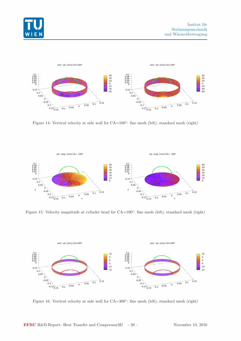
outward of the valve pocket . . . . . . . . . . . . . . . . . . . . . . . . . . . . . . . . . . . 1914 Vertical velocity at side wall for CA=100◦: fine mesh (left), standard mesh (right) . . . . 2015 Velocity magnitude at cylinder head for CA=100◦: fine mesh (left), standard mesh (right) 2016 Vertical velocity at side wall for CA=300◦: fine mesh (left), standard mesh (right) . . . . 2017 Heat transfer coefficient. Numerical results for fine and standard mesh . . . . . . . . . . . 2118 Pressure . . . . . . . . . . . . . . . . . . . . . . . . . . . . . . . . . . . . . . . . . . . . . . 2219 Valve lift discharge valves . . . . . . . . . . . . . . . . . . . . . . . . . . . . . . . . . . . . 2320 Velocity at Piston CA=420◦ . . . . . . . . . . . . . . . . . . . . . . . . . . . . . . . . . . 2321 Pressure at piston CA=306◦ . . . . . . . . . . . . . . . . . . . . . . . . . . . . . . . . . . 2422 Temperature at side wall CA=504◦ . . . . . . . . . . . . . . . . . . . . . . . . . . . . . . . 24

List of Tables

1 Structure of .msh file . . . . . . . . . . . . . . . . . . . . . . . . . . . . . . . . . . . . . . . 72 Output-data in File Output.txt . . . . . . . . . . . . . . . . . . . . . . . . . . . . . . . . . 133 Output-data in File Output.txt, Valve numbering: suction valves iV = 1,...,nSV ; discharge

valves iV = nSV +1,...,nSV +nDV , nSV number of suction valves, nDV number of dischargevalves, order according to list in “InputCylinder.txt” or GUI, resp.. . . . . . . . . . . . . 13

4 Cylinder data . . . . . . . . . . . . . . . . . . . . . . . . . . . . . . . . . . . . . . . . . . . 145 Numerical parameters . . . . . . . . . . . . . . . . . . . . . . . . . . . . . . . . . . . . . . 146 Data suction valves . . . . . . . . . . . . . . . . . . . . . . . . . . . . . . . . . . . . . . . . 157 Data discharge valves . . . . . . . . . . . . . . . . . . . . . . . . . . . . . . . . . . . . . . 158 Dimensions of valve pocket . . . . . . . . . . . . . . . . . . . . . . . . . . . . . . . . . . . 159 Computation time for standard and fine mesh for 2-valve compressor . . . . . . . . . . . . 15

EFRC R&D-Report: Heat Transfer and Compressor3D - 2 - November 10, 2016



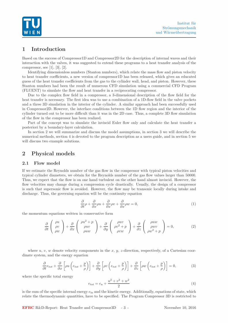
1 Introduction

Based on the success of Compressor1D and Compressor2D for the description of internal waves and theirinteraction with the valves, it was suggested to extend these programs to a heat transfer analysis of thecompressor, see [1], [3], [2].

Identifying dimensionless numbers (Stanton numbers), which relate the mass flow and piston velocityto heat transfer coefficients, a new version of compressor1D has been released, which gives an educatedguess of the heat transfer coefficients from the gas to the cylinder wall, head, and piston. However, theseStanton numbers had been the result of numerous CFD simulation using a commercial CFD Program(FLUENT) to simulate the flow and heat transfer in a reciprocating compressor.

Due to the complex flow field in a compressor, a 3-dimensional description of the flow field for theheat transfer is necessary. The first idea was to use a combination of a 1D-flow field in the valve pocketsand a three 3D simulation in the interior of the cylinder. A similar approach had been successfully usedin Compressor2D. However, the interface conditions between the 1D flow region and the interior of thecylinder turned out to be more difficult than it was in the 2D case. Thus, a complete 3D flow simulationof the flow in the compressor has been realized.

Part of the concept was to simulate the inviscid Euler flow only and calculate the heat transfer aposteriori by a boundary-layer calculation.

In section 2 we will summarize and discuss the model assumptions, in section 3 we will describe thenumerical methods, section 4 is devoted to the program description as a users guide, and in section 5 wewill discuss two example solutions.

2 Physical models

2.1 Flow model

If we estimate the Reynolds number of the gas flow in the compressor with typical piston velocities andtypical cylinder diameters, we obtain for the Reynolds number of the gas flow values larger than 50000.Thus, we expect that the flow is on one hand turbulent on the other hand almost inviscid. However, theflow velocities may change during a compression cycle drastically. Usually, the design of a compressoris such that supersonic flow is avoided. However, the flow may be transonic locally during intake anddischarge. Thus, the governing equation will be the continuity equation

∂

∂tρ +

∂

∂xρu +

∂

∂xρv +

∂

∂xρw = 0, (1)

the momentum equations written in conservative form

∂

∂t

ρuρvρw

+∂

∂x

ρu2 + pρuvρuw

+∂

∂y

ρuvρv2 + p

ρvw

+∂

∂z

ρuwρwv

ρw2 + p

= 0, (2)

where u, v, w denote velocity components in the x, y, z-direction, respectively, of a Cartesian coor-dinate system, and the energy equation

∂

∂tetot +

∂

∂x

[

ρu

(

etot +p

ρ

)]

+∂

∂y

[

ρv

(

etot +p

ρ

)]

+∂

∂z

[

ρw

(

etot +p

ρ

)]

= 0, (3)

where the specific total energy

etot = en +u2 + v2 + w2

2(4)

is the sum of the specific internal energy ein and the kinetic energy. Additionally, equations of state, whichrelate the thermodynamic quantities, have to be specified. The Program Compressor 3D is restricted to




ideal gases with constant specific heat capacities.

p

ρ= (cp − cv)T, ein = cvT, (5)

where cv. cp are the specific iso-choric and iso-baric specific heat capacities, respectively. The absolutetemperature is denoted by T .

2.2 Valve model

2.2.1 Valve Dynamic

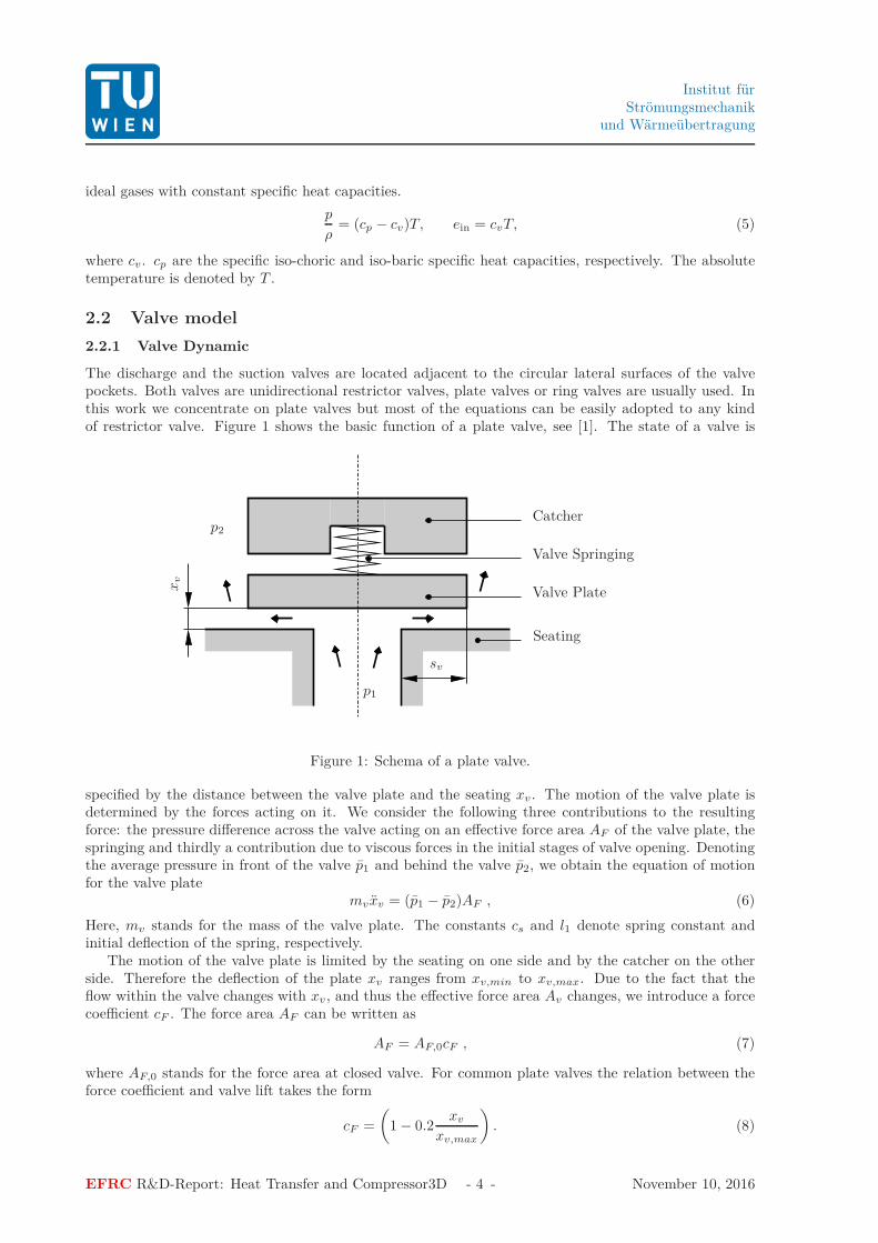
The discharge and the suction valves are located adjacent to the circular lateral surfaces of the valvepockets. Both valves are unidirectional restrictor valves, plate valves or ring valves are usually used. Inthis work we concentrate on plate valves but most of the equations can be easily adopted to any kindof restrictor valve. Figure 1 shows the basic function of a plate valve, see [1]. The state of a valve is

p1

p2

Seating

Valve Platexv

sv

Catcher

Valve Springing

Figure 1: Schema of a plate valve.

specified by the distance between the valve plate and the seating xv. The motion of the valve plate isdetermined by the forces acting on it. We consider the following three contributions to the resultingforce: the pressure difference across the valve acting on an effective force area AF of the valve plate, thespringing and thirdly a contribution due to viscous forces in the initial stages of valve opening. Denotingthe average pressure in front of the valve p1 and behind the valve p2, we obtain the equation of motionfor the valve plate

mvxv = (p1 − p2)AF , (6)

Here, mv stands for the mass of the valve plate. The constants cs and l1 denote spring constant andinitial deflection of the spring, respectively.

The motion of the valve plate is limited by the seating on one side and by the catcher on the otherside. Therefore the deflection of the plate xv ranges from xv,min to xv,max. Due to the fact that theflow within the valve changes with xv, and thus the effective force area Av changes, we introduce a forcecoefficient cF . The force area AF can be written as

AF = AF,0cF , (7)

where AF,0 stands for the force area at closed valve. For common plate valves the relation between theforce coefficient and valve lift takes the form

cF =

(

1 − 0.2xv

xv,max

)

. (8)




2.2.2 Flow through the valve

The flow through the valves is considered as (quasi stationary) outflow of gas from a pressurized vesselthrough a convergent nozzle. In case of constant heat capacities the mass flow density j is given bySt.Venant and Wantzell [5]

j = m =1

AV

φρ1

(p2

pt1

) 1

γ

√√√√ 2γ

γ − 1

pt1

ρ1

(

1 −

(p2

pt1

) γ−1

γ

)

, (9)

where AV is the valve cross section and pt1 are the total pressures before and p2 is the pressures afterthe valve, respectively. Note, p2 and pt may vary along the valve.

The effective flow cross section φ of the valve is assumed to be a function of the position of the valveplate xv only. This is not true if effects of asymmetric flow conditions in the valve pocket are taken intoaccount. For common valves the equation for the effective cross section takes the form

φ(xv) =

√

(fe1mmxv)2

αv + βvxv2

. (10)

The constant fe1mm denotes the valve flow cross-section when the valve plate is 1 mm above the valveseating. The constants αv and βv describe non-linear dependencies of the valve plate lift and have to bedetermined empirically.

2.3 Heat transfer model

The heat transfer coefficients will be calculated as a post processing of the inviscid Euler-flow simulation.Thus, we have implicitly assumed that the heat transfer from outside to the core region of the flow doesnot influence the flow field, the pressure, and density distribution. For the heat transfer analysis weassume that the internal (inviscid) flow field is given and the heat transfer to the cylinder wall, pistonand cylinder head will be determined by a posteriori boundary-layer calculation.

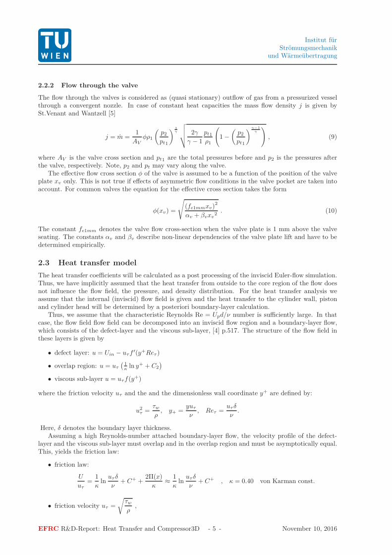
Thus, we assume that the characteristic Reynolds Re = Upd/ν number is sufficiently large. In thatcase, the flow field flow field can be decomposed into an inviscid flow region and a boundary-layer flow,which consists of the defect-layer and the viscous sub-layer, [4] p.517. The structure of the flow field inthese layers is given by

• defect layer: u = Uin − uτ f ′(y+Reτ )

• overlap region: u = uτ

(1

κln y+ + C2

)

• viscous sub-layer u = uτ f(y+)

where the friction velocity uτ and the and the dimensionless wall coordinate y+ are defined by:

u2τ =

τw

ρ, y+ =

yuτ

ν, Reτ =

uτ δ

ν.

Here, δ denotes the boundary layer thickness.Assuming a high Reynolds-number attached boundary-layer flow, the velocity profile of the defect-

layer and the viscous sub-layer must overlap and in the overlap region and must be asymptotically equal.This, yields the friction law:

• friction law:

U

uτ

=1

κln

uτ δ

ν+ C+ +

2Π(x)

κ≈

1

κln

uτ δ

ν+ C+ , κ = 0.40 von Karman const.

• friction velocity uτ =

√τw

ρ,




Uin

defect layerviscous sub−layer

overlap region

inviscid flow

τwwq

inT

Tw

δ

Figure 2: Structure of an attached turbulent boundary-layer

• friction coefficient: cf =2τw

ρU2= 2

u2τ

U2.

The constant C+ depends on the velocity profile in the viscous sub-laver and is a function of the wallroughness only. Π(x) depends on the velocity profile in the defect layer and δ is the yet unknown boundarylayer thickness.

In order to determine the missing quantities one has to solve the boundary-layer equation in the defectregion. The following three strategies can be followed:

a) Solve the boundary-layer equations (finite volume method). A turbulence model has to be chosen.

b) Solve boundary-layer equations with an integral method for δ. A suitable velocity profile has to bechosen.

c) Estimate boundary layer thickness for each face.

For simplicity we have chosen strategy c) assuming the simplest boundary-layer structure see [4] p.581.

cf = 2

κ

ln ReG(Λ,D)︸︷︷︸

∼1.5

2

(11)

Using the Reynolds analogy for the heat transfer, we obtain for the heat transfer coefficient, see [4](18.157]

αave = ρcpUaveSt, St =1

Prt

cf

2,

where St is the Stanton number which relates the wall heat flux density q to an appropriate enthalpyflux density ρucp∆T based on the inviscid flow velocity along the wall. The turbulent Prandtl numberis assumed to be constant, Prt = 0.87. The velocity uave is the momentary mean velocity of the inviscidflow field over the the face (piston, head, side wall) under consideration.

The heat transfer coefficients are stored in the file alpha_on_HSP.txt.

2.3.1 Release note 23.4.2015

The current version of Compressor3D calculates the average heat transfer coefficients for each face (piston,head and side wall) as a function of the crank angle. At the moment the material properties of the gasare hard coded for air. In a later version an option to choose the material properties will be included.

3 Numerical issues

3.1 Geometry and mesh

The domain of the flow simulation consists of the interior of the compressor between the cylinder headand the movable piston and a (variable) number of valve pockets which connect the the cylinder with thevalves.




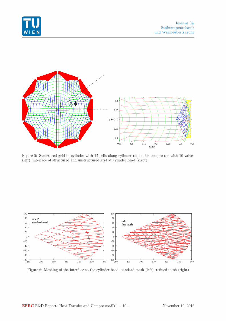
3.1.1 Cylinder

Due to the simple geometry of the cylinder inside the cylinder a layered structured mesh is used. Thegrid lines in the plane of the cylinder head are shown in figure 5 for a compressor with 5 suction and 5discharge valves. In this example there are nR = 15 cells along the radius of the cylinder. In the verticaldirection (along the cylinder axis) the cell size depends on the piston of the cylinder. The cells are evenlydistributed in vertical direction. If the the aspect ratio of the cells are below or above certain thresholds,a new mesh will be generated and the cell averages of the computational quantities will be redistributedto the new cells in a conservative manner. The minimum number of cells in z−direction is 2, when thepiston in the position of minimal volume.

3.1.2 Valve Pockets

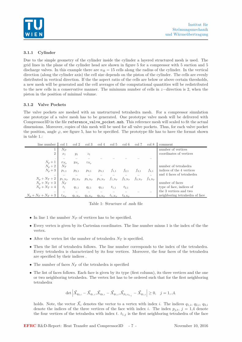
The valve pockets are meshed with an unstructured tetrahedra mesh. For a compressor simulationone prototype of a valve mesh has to be generated. One prototype valve mesh will be delivered withCompressor3D in the file reference_valve_pocket.msh. This reference mesh will scaled to fit the actualdimensions. Moreover, copies of this mesh will be used for all valve pockets. Thus, for each valve pocketthe position, angle ϕ, see figure 5, has to be specified. The prototype file has to have the format shownin table 1.:

line number col 1 col 2 col 3 col 4 col 5 col 6 col 7 col 8 comment

1 NP number of vertices2 x1 y1 z1 coordinates of vertices. .. .. .. .. .. .. .. ..

Np + 1 xNpyNp

zNp

Np + 2 NT number of tetrahedraNp + 3 p1,1 p2,1 p3,1 p4,1 f1,1 f2,1 f3,1 f4,1 indices of the 4 vertices

.. .. .. .. .. .. .. .. .. and 4 faces of tetrahedraNp + NT + 2 p1,NT

p2,NTp3,NT

p4,NTf1,NT

f2,NTf3,NT

f4,NT

Np + NT + 3 NF number of facesNp + NT + 4 t1 q1,1 q2,1 q3,1 t1,1 t2,1 type of face, indices of

.. .. .. .. .. .. .. .. .. the 3 vertices and twoNp + NT + NF + 3 tNF

q1,NFq2,NF

q3,NFt1,NF

t2,NFneighboring tetrahedra of face

Table 1: Structure of .msh file

• In line 1 the number NP of vertices has to be specified.

• Every vertex is given by its Cartesian coordinates. The line number minus 1 is the index of the thevertex.

• After the vertex list the number of tetrahedra NT is specified.

• Then the list of tetrahedra follows. The line number corresponds to the index of the tetrahedra.Every tetrahedra is characterized by its four vertices. Moreover, the four faces of the tetrahedraare specified by their indices .

• The number of faces NF of the tetrahedra is specified

• The list of faces follows. Each face is given by its type (first column), its three vertices and the oneor two neighboring tetrahedra. The vertex list has to be ordered such that for the first neighboringtetrahedra

det∣∣∣ ~Xq2,i

− ~Xq1,i, ~Xq3,i

− ~Xq1,i, ~Xpj,t1,i

− ~Xq1,i

∣∣∣ ≥ 0, j = 1,.,4.

holds. Note, the vector ~Xi denotes the vector to a vertex with index i. The indices q1,i, q2,i, q3,i

denote the indices of the three vertices of the face with index i. The index pj,t, j = 1,4 denotethe four vertices of the tetrahedra with index t. t1,j is the first neighboring tetrahedra of the face




with index i. Note, if one of the tetrahedra vertices is on the face, the determinant vanishes. Onlyfor the fourth point it is nonzero. In order to guarantee that the numerical fluxes at the faceshave the correct sign, the tetrahedra must be oriented such that this determinant is positive. As aconsequence, the determinant for the second tetrahedra is negative.

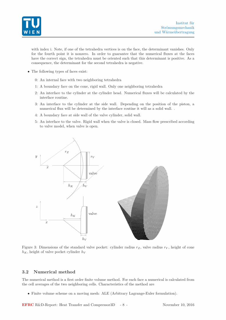
• The following types of faces exist:

0: An internal face with two neighboring tetrahedra

1: A boundary face on the cone, rigid wall. Only one neighboring tetrahedra

2: An interface to the cylinder at the cylinder head. Numerical fluxes will be calculated by theinterface routine.

3: An interface to the cylinder at the side wall. Depending on the position of the piston, anumerical flux will be determined by the interface routine it will as a solid wall. .

4: A boundary face at side wall of the valve cylinder, solid wall.

5: An interface to the valve. Rigid wall when the valve is closed. Mass flow prescribed accordingto valve model, when valve is open.

rV

rZ

hV

hVhK

hK

x

x

y

z

valve

valve

Figure 3: Dimensions of the standard valve pocket: cylinder radius rZ , valve radius rV , height of conehK , height of valve pocket cylinder hV

3.2 Numerical method

The numerical method is a first order finite volume method. For each face a numerical is calculated fromthe cell averages of the two neighboring cells. Characteristics of the method are

• Finite volume scheme on a moving mesh: ALE (Arbitrary Lagrange-Euler formulation).




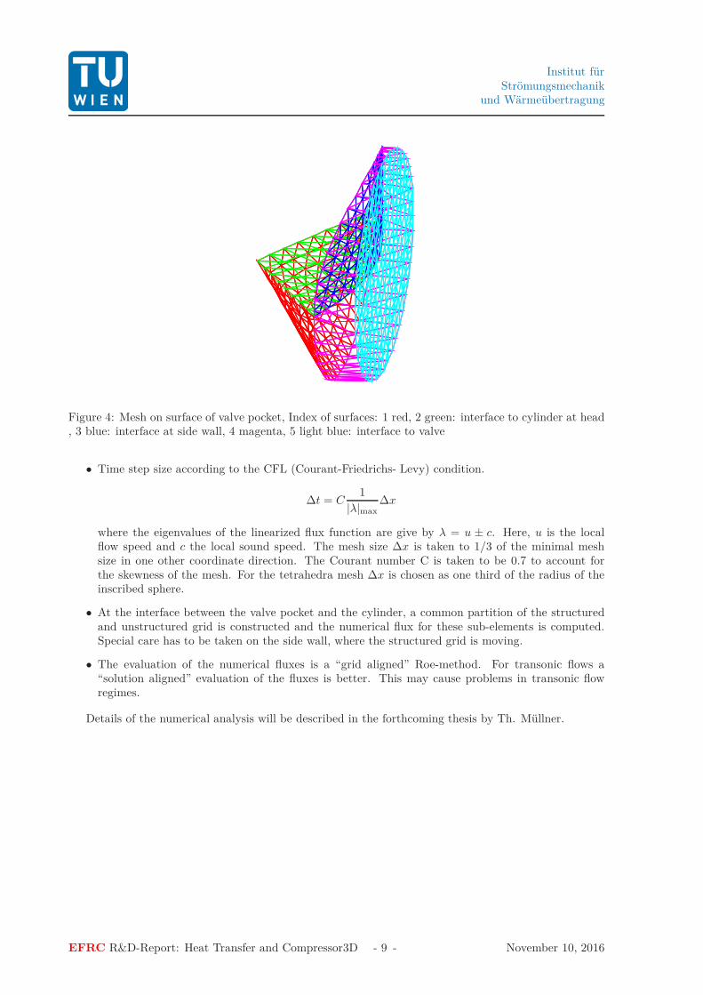
Figure 4: Mesh on surface of valve pocket, Index of surfaces: 1 red, 2 green: interface to cylinder at head, 3 blue: interface at side wall, 4 magenta, 5 light blue: interface to valve

• Time step size according to the CFL (Courant-Friedrichs- Levy) condition.

∆t = C1

|λ|max

∆x

where the eigenvalues of the linearized flux function are give by λ = u ± c. Here, u is the localflow speed and c the local sound speed. The mesh size ∆x is taken to 1/3 of the minimal meshsize in one other coordinate direction. The Courant number C is taken to be 0.7 to account forthe skewness of the mesh. For the tetrahedra mesh ∆x is chosen as one third of the radius of theinscribed sphere.

• At the interface between the valve pocket and the cylinder, a common partition of the structuredand unstructured grid is constructed and the numerical flux for these sub-elements is computed.Special care has to be taken on the side wall, where the structured grid is moving.

• The evaluation of the numerical fluxes is a “grid aligned” Roe-method. For transonic flows a“solution aligned” evaluation of the fluxes is better. This may cause problems in transonic flowregimes.

Details of the numerical analysis will be described in the forthcoming thesis by Th. Müllner.




ϕ

x(m)

y (m)

−0.1

−0.05

0

0.05

0.1

0.05 0.1 0.15 0.2 0.25 0.3 0.35

Figure 5: Structured grid in cylinder with 15 cells along cylinder radius for compressor with 10 valves(left), interface of structured and unstructured grid at cylinder head (right)

side 2standard mesh side

fine mesh

−100

−80

−60

−40

−20

0

20

40

60

80

100

280 290 300 310 320 330 340−100

−80

−60

−40

−20

0

20

40

60

80

100

280 290 300 310 320 330 340

Figure 6: Meshing of the interface to the cylinder head standard mesh (left), refined mesh (right)




4 Program description and handing

4.1 Installation

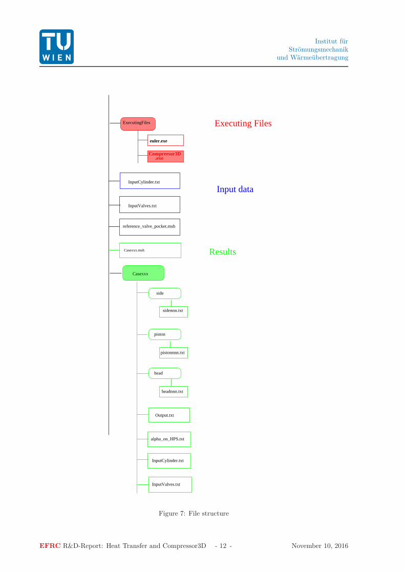
The The setup file for the program can be downloaded from http://www.fluid.tuwien.ac.at/efrc. Exe-cuting setup.exe installs the program in a directory which can be chosen. We call it the root directoryof the program. The root directory contains a subdirectory called “ExecutingFiles”. Here resides“Compressor3D.exe” By clicking onto “Compressor3D.exe” a GUI (Graphical User Interface) opens.The program can only be used if a valid license is provided. Click on the item “license”, then you willget your license status. If no valid license is issued. send the number in the field “licensing information”to the authors of the program. If your are a legitimate user you will get the necessary license key. Thelicense key is only valid for the specific computer and stored in the file “license.dat”.

4.2 Using the Program

Call the program by clicking onto Compressor3D.exe in “ExecutingFiles”. You can fill out all fields in theGUI or read input files for the cylinder data (see tables 4,5 and the valve data, see tables 6,7,8. Thesedata files can be saved unter the item “File” “Save Valve Data”, “Save Cylinder Data”. figure 7

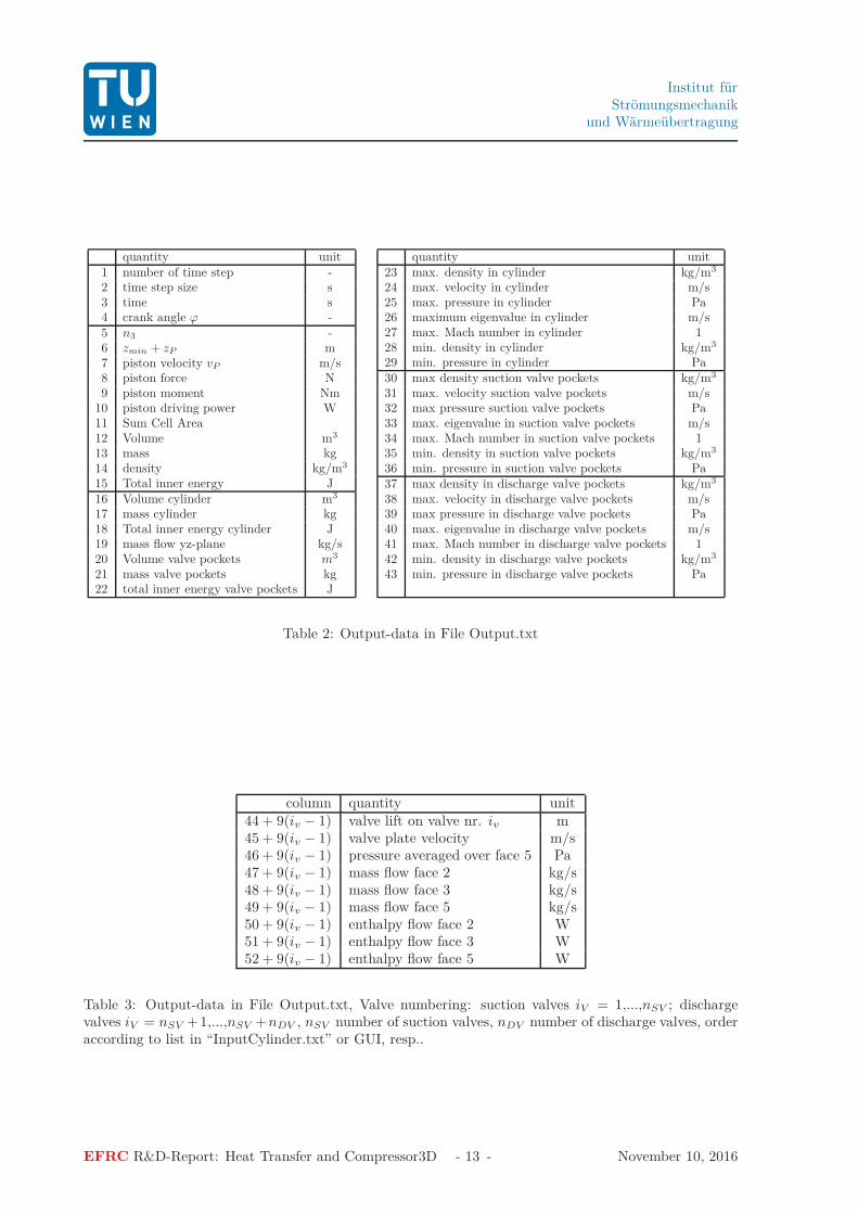
For the calculation switch to “Calculation” and enter a case-name. A subdirectory of the root directorywith the case-name will be created, if it does not already exist. All information of the current case willbe written into this directory. A copy of the cylinder data, valve data and a file named “Output.txt”which contains information for every time step. The meaning of the data in “Output.txt” is listed in thetables 2, 3.

4.3 Changing the unstructured mesh

The reference mesh for the valve pocket is the file reference_valve_pocket.msh” in the root directory.If you want to change it, rename your new mesh file to “reference_valve_pocket.msh” and put it in theroot directory. A fine mesh for the valve pocket is available on the web site.

The name of the mesh file which you enter in the GUI is for internal use only. This file will containthe scaled mesh.

Please note that the program does not check for geometrical conflicts regarding the angular distancebetween neighboring valve or the deformation of the reference valve pocket.

4.4 Post Processing

The output of the program are the following files:

• “Casedir/Output.txt see table 2, 3

• “Casedir/head/headxxx.txt”

“Casedir/side/sidexxx.txt”

“Casedir/piston/pistonxxx.txt”

where xxx is the crank angle.

• If you press heat “Plot heat transfer” the heat transfer coefficients for every side will be calculatedand stored in “Casedir/alpha_on_HPS.txt”, and displayed.

• With the button “Plot head/piston/side results” plots of the pressure, density and velocity field onthe piston, head and side wall will be generated and stored as .png files in the respective directories.

• For further plots of the data the freely available plot program “gnuplot” can be used. This programresides also in “ExecutingFiles”. A description of gnuplot can be found at http://www.gnuplot.info/.




Casexxx

headnnn.txt

pistonnnn.txt

sidennn.txt

side

piston

head

Output.txt

InputCylinder.txt

InputValves.txt

alpha_on_HPS.txt

ExecutingFiles

Input data

Executing Files

Compreesor3D.exe

euler.exe

InputCylinder.txt

InputValves.txt

reference_valve_pocket.msh

Casexxx.msh Results

Figure 7: File structure




quantity unit1 number of time step -2 time step size s3 time s4 crank angle ϕ -5 n3 -6 zmin + zP m7 piston velocity vP m/s8 piston force N9 piston moment Nm

10 piston driving power W11 Sum Cell Area12 Volume m3

13 mass kg14 density kg/m3

15 Total inner energy J16 Volume cylinder m3

17 mass cylinder kg18 Total inner energy cylinder J19 mass flow yz-plane kg/s20 Volume valve pockets m3

21 mass valve pockets kg22 total inner energy valve pockets J

quantity unit23 max. density in cylinder kg/m3

24 max. velocity in cylinder m/s25 max. pressure in cylinder Pa26 maximum eigenvalue in cylinder m/s27 max. Mach number in cylinder 128 min. density in cylinder kg/m3

29 min. pressure in cylinder Pa30 max density suction valve pockets kg/m3

31 max. velocity suction valve pockets m/s32 max pressure suction valve pockets Pa33 max. eigenvalue in suction valve pockets m/s34 max. Mach number in suction valve pockets 135 min. density in suction valve pockets kg/m3

36 min. pressure in suction valve pockets Pa37 max density in discharge valve pockets kg/m3

38 max. velocity in discharge valve pockets m/s39 max pressure in discharge valve pockets Pa40 max. eigenvalue in discharge valve pockets m/s41 max. Mach number in discharge valve pockets 142 min. density in discharge valve pockets kg/m3

43 min. pressure in discharge valve pockets Pa

Table 2: Output-data in File Output.txt

column quantity unit44 + 9(iv − 1) valve lift on valve nr. iv m45 + 9(iv − 1) valve plate velocity m/s46 + 9(iv − 1) pressure averaged over face 5 Pa47 + 9(iv − 1) mass flow face 2 kg/s48 + 9(iv − 1) mass flow face 3 kg/s49 + 9(iv − 1) mass flow face 5 kg/s50 + 9(iv − 1) enthalpy flow face 2 W51 + 9(iv − 1) enthalpy flow face 3 W52 + 9(iv − 1) enthalpy flow face 5 W

Table 3: Output-data in File Output.txt, Valve numbering: suction valves iV = 1,...,nSV ; dischargevalves iV = nSV +1,...,nSV +nDV , nSV number of suction valves, nDV number of discharge valves, orderaccording to list in “InputCylinder.txt” or GUI, resp..




5 Examples

5.1 Two valve compressor

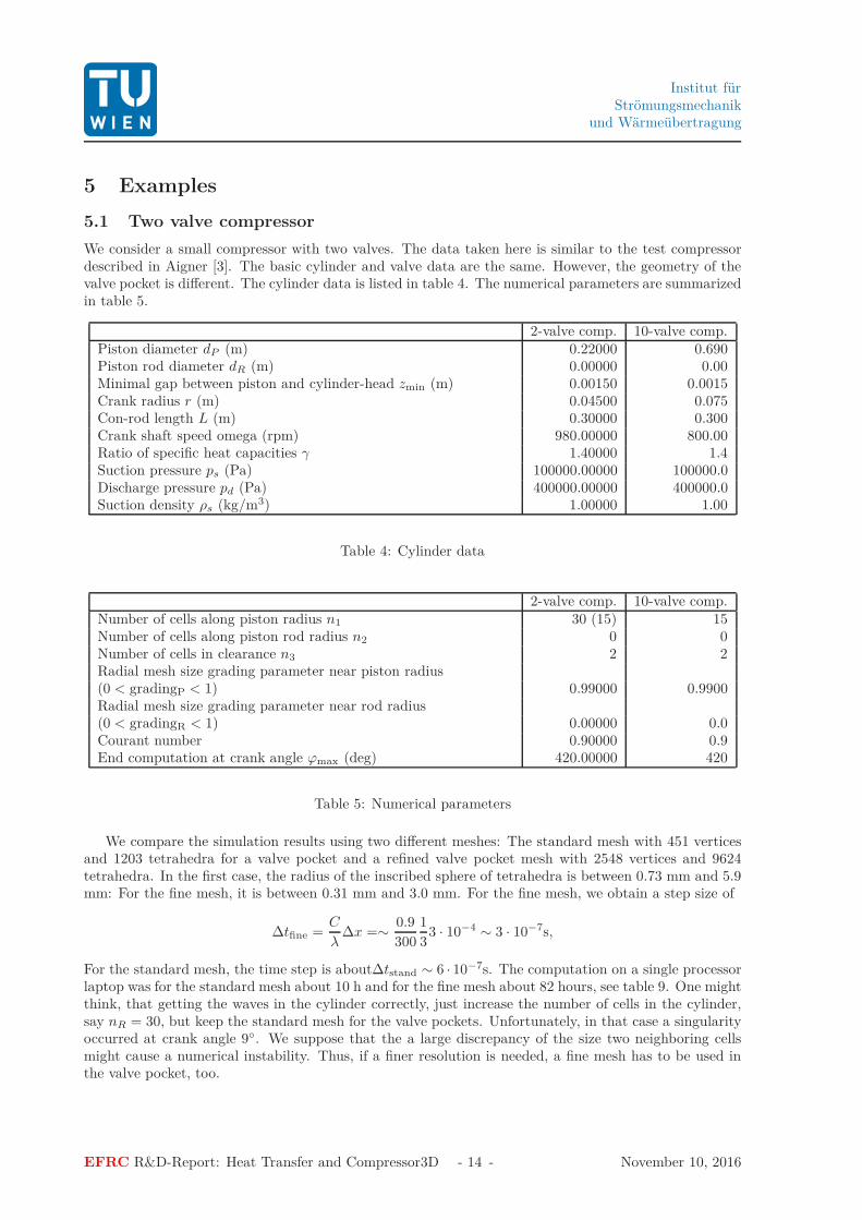
We consider a small compressor with two valves. The data taken here is similar to the test compressordescribed in Aigner [3]. The basic cylinder and valve data are the same. However, the geometry of thevalve pocket is different. The cylinder data is listed in table 4. The numerical parameters are summarizedin table 5.

2-valve comp. 10-valve comp.Piston diameter dP (m) 0.22000 0.690Piston rod diameter dR (m) 0.00000 0.00Minimal gap between piston and cylinder-head zmin (m) 0.00150 0.0015Crank radius r (m) 0.04500 0.075Con-rod length L (m) 0.30000 0.300Crank shaft speed omega (rpm) 980.00000 800.00Ratio of specific heat capacities γ 1.40000 1.4Suction pressure ps (Pa) 100000.00000 100000.0Discharge pressure pd (Pa) 400000.00000 400000.0Suction density ρs (kg/m3) 1.00000 1.00

Table 4: Cylinder data

2-valve comp. 10-valve comp.Number of cells along piston radius n1 30 (15) 15Number of cells along piston rod radius n2 0 0Number of cells in clearance n3 2 2Radial mesh size grading parameter near piston radius(0 < gradingP < 1) 0.99000 0.9900Radial mesh size grading parameter near rod radius(0 < gradingR < 1) 0.00000 0.0Courant number 0.90000 0.9End computation at crank angle ϕmax (deg) 420.00000 420

Table 5: Numerical parameters

We compare the simulation results using two different meshes: The standard mesh with 451 verticesand 1203 tetrahedra for a valve pocket and a refined valve pocket mesh with 2548 vertices and 9624tetrahedra. In the first case, the radius of the inscribed sphere of tetrahedra is between 0.73 mm and 5.9mm: For the fine mesh, it is between 0.31 mm and 3.0 mm. For the fine mesh, we obtain a step size of

∆tfine =C

λ∆x =∼

0.9

300

1

33 · 10−4 ∼ 3 · 10−7s,

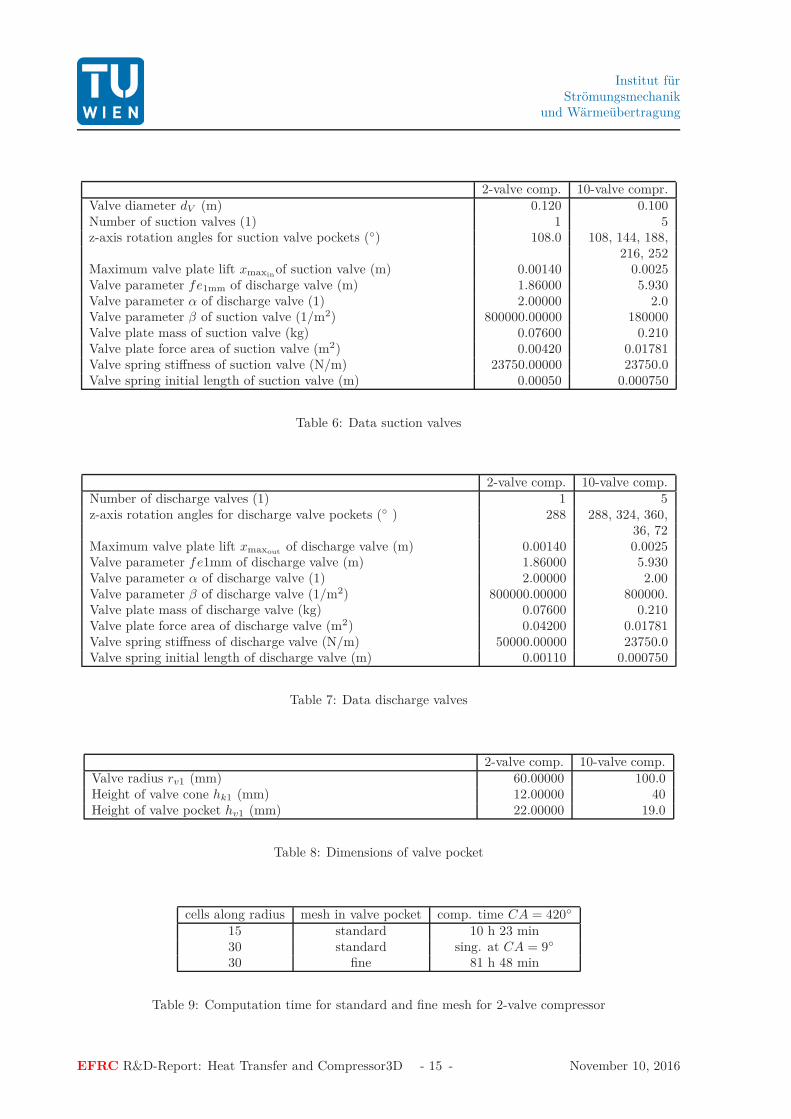
For the standard mesh, the time step is about∆tstand ∼ 6 · 10−7s. The computation on a single processorlaptop was for the standard mesh about 10 h and for the fine mesh about 82 hours, see table 9. One mightthink, that getting the waves in the cylinder correctly, just increase the number of cells in the cylinder,say nR = 30, but keep the standard mesh for the valve pockets. Unfortunately, in that case a singularityoccurred at crank angle 9◦. We suppose that the a large discrepancy of the size two neighboring cellsmight cause a numerical instability. Thus, if a finer resolution is needed, a fine mesh has to be used inthe valve pocket, too.




2-valve comp. 10-valve compr.Valve diameter dV (m) 0.120 0.100Number of suction valves (1) 1 5z-axis rotation angles for suction valve pockets (◦) 108.0 108, 144, 188,

216, 252Maximum valve plate lift xmaxin

of suction valve (m) 0.00140 0.0025Valve parameter fe1mm of discharge valve (m) 1.86000 5.930Valve parameter α of discharge valve (1) 2.00000 2.0Valve parameter β of suction valve (1/m2) 800000.00000 180000Valve plate mass of suction valve (kg) 0.07600 0.210Valve plate force area of suction valve (m2) 0.00420 0.01781Valve spring stiffness of suction valve (N/m) 23750.00000 23750.0Valve spring initial length of suction valve (m) 0.00050 0.000750

Table 6: Data suction valves

2-valve comp. 10-valve comp.Number of discharge valves (1) 1 5z-axis rotation angles for discharge valve pockets (◦ ) 288 288, 324, 360,

36, 72Maximum valve plate lift xmaxout

of discharge valve (m) 0.00140 0.0025Valve parameter fe1mm of discharge valve (m) 1.86000 5.930Valve parameter α of discharge valve (1) 2.00000 2.00Valve parameter β of discharge valve (1/m2) 800000.00000 800000.Valve plate mass of discharge valve (kg) 0.07600 0.210Valve plate force area of discharge valve (m2) 0.04200 0.01781Valve spring stiffness of discharge valve (N/m) 50000.00000 23750.0Valve spring initial length of discharge valve (m) 0.00110 0.000750

Table 7: Data discharge valves

2-valve comp. 10-valve comp.Valve radius rv1 (mm) 60.00000 100.0Height of valve cone hk1 (mm) 12.00000 40Height of valve pocket hv1 (mm) 22.00000 19.0

Table 8: Dimensions of valve pocket

cells along radius mesh in valve pocket comp. time CA = 420◦

15 standard 10 h 23 min30 standard sing. at CA = 9◦

30 fine 81 h 48 min

Table 9: Computation time for standard and fine mesh for 2-valve compressor




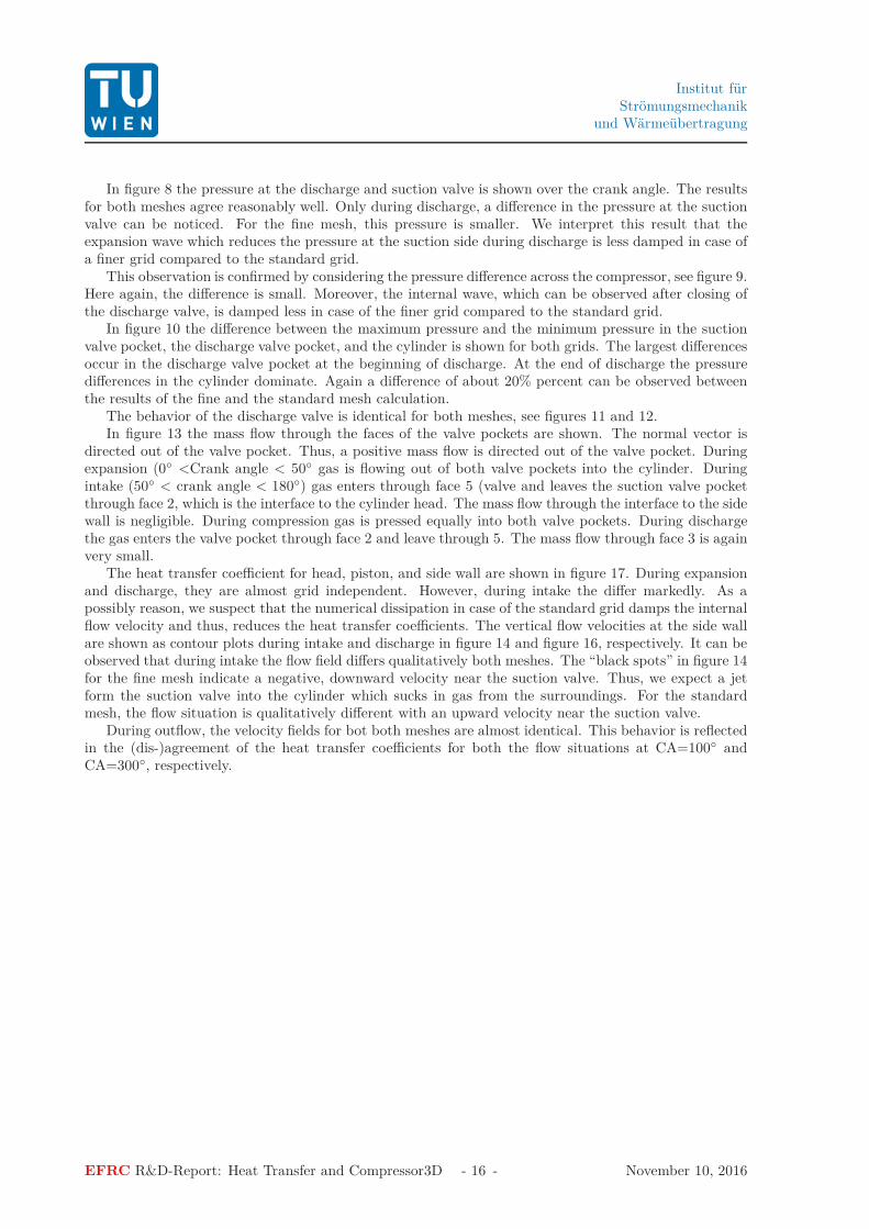
In figure 8 the pressure at the discharge and suction valve is shown over the crank angle. The resultsfor both meshes agree reasonably well. Only during discharge, a difference in the pressure at the suctionvalve can be noticed. For the fine mesh, this pressure is smaller. We interpret this result that theexpansion wave which reduces the pressure at the suction side during discharge is less damped in case ofa finer grid compared to the standard grid.

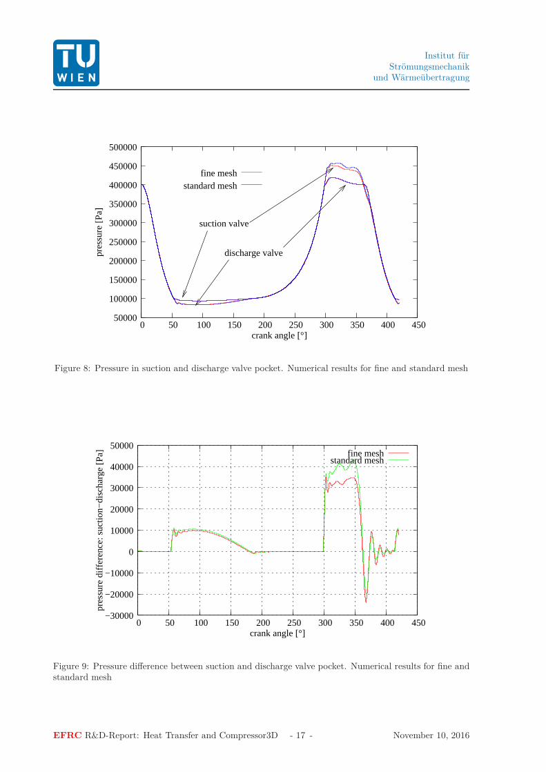
This observation is confirmed by considering the pressure difference across the compressor, see figure 9.Here again, the difference is small. Moreover, the internal wave, which can be observed after closing ofthe discharge valve, is damped less in case of the finer grid compared to the standard grid.

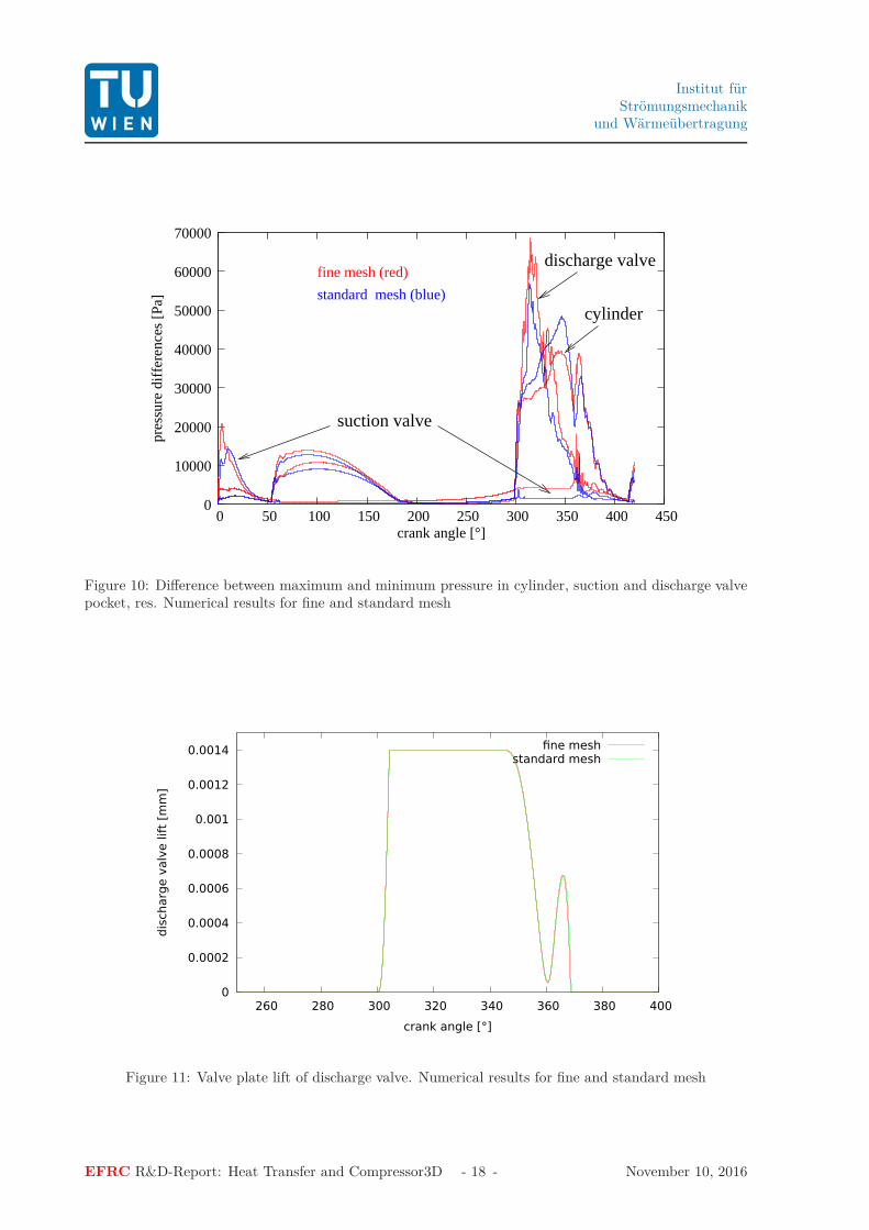
In figure 10 the difference between the maximum pressure and the minimum pressure in the suctionvalve pocket, the discharge valve pocket, and the cylinder is shown for both grids. The largest differencesoccur in the discharge valve pocket at the beginning of discharge. At the end of discharge the pressuredifferences in the cylinder dominate. Again a difference of about 20% percent can be observed betweenthe results of the fine and the standard mesh calculation.

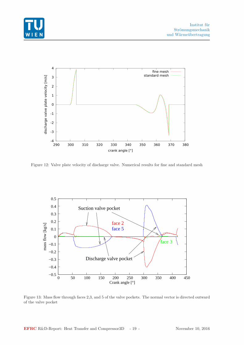
The behavior of the discharge valve is identical for both meshes, see figures 11 and 12.In figure 13 the mass flow through the faces of the valve pockets are shown. The normal vector is

directed out of the valve pocket. Thus, a positive mass flow is directed out of the valve pocket. Duringexpansion (0◦ <Crank angle < 50◦ gas is flowing out of both valve pockets into the cylinder. Duringintake (50◦ < crank angle < 180◦) gas enters through face 5 (valve and leaves the suction valve pocketthrough face 2, which is the interface to the cylinder head. The mass flow through the interface to the sidewall is negligible. During compression gas is pressed equally into both valve pockets. During dischargethe gas enters the valve pocket through face 2 and leave through 5. The mass flow through face 3 is againvery small.

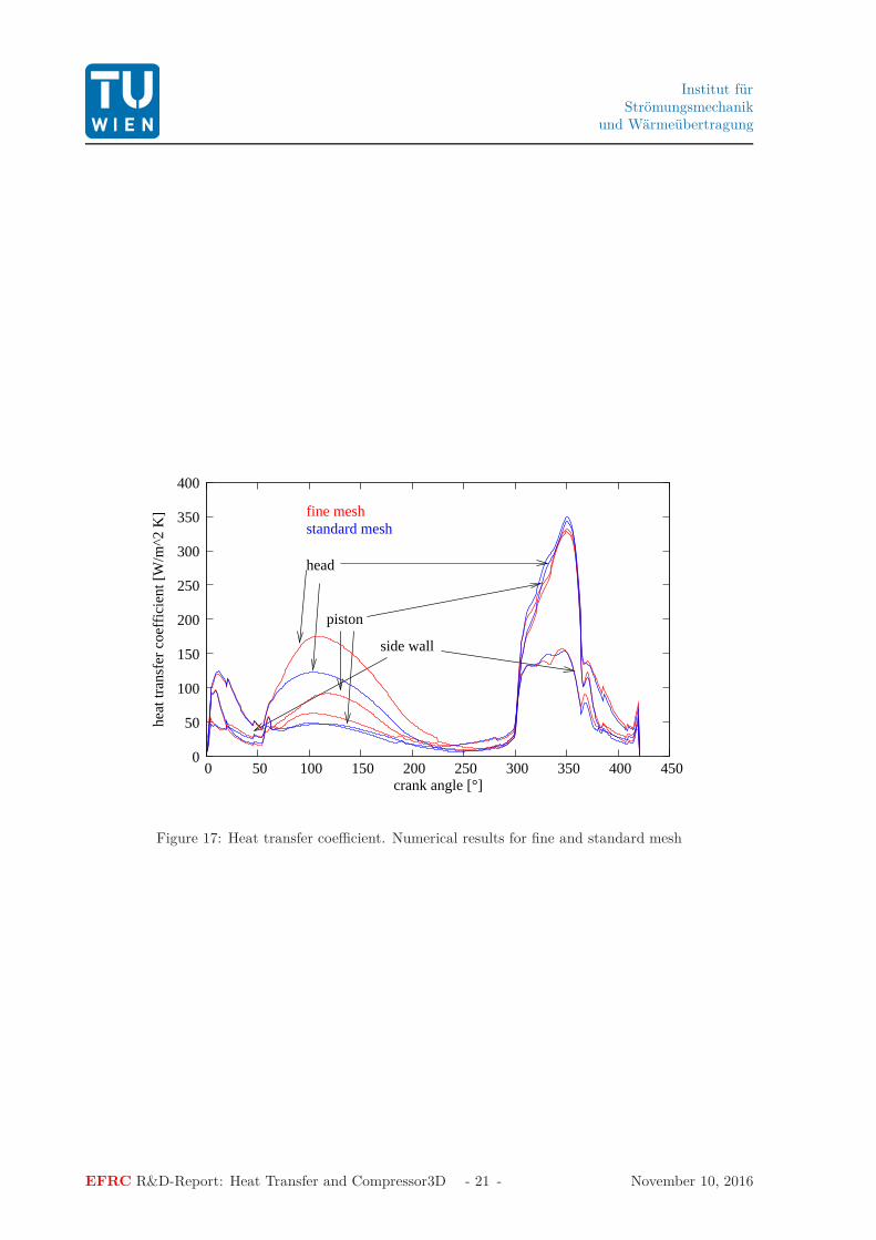
The heat transfer coefficient for head, piston, and side wall are shown in figure 17. During expansionand discharge, they are almost grid independent. However, during intake the differ markedly. As apossibly reason, we suspect that the numerical dissipation in case of the standard grid damps the internalflow velocity and thus, reduces the heat transfer coefficients. The vertical flow velocities at the side wallare shown as contour plots during intake and discharge in figure 14 and figure 16, respectively. It can beobserved that during intake the flow field differs qualitatively both meshes. The “black spots” in figure 14for the fine mesh indicate a negative, downward velocity near the suction valve. Thus, we expect a jetform the suction valve into the cylinder which sucks in gas from the surroundings. For the standardmesh, the flow situation is qualitatively different with an upward velocity near the suction valve.

During outflow, the velocity fields for bot both meshes are almost identical. This behavior is reflectedin the (dis-)agreement of the heat transfer coefficients for both the flow situations at CA=100◦ andCA=300◦, respectively.




suction valve

discharge valve

50000

100000

150000

200000

250000

300000

350000

400000

450000

500000

0 50 100 150 200 250 300 350 400 450

pres

sure

[Pa]

fine mesh

crank angle [°]

standard mesh

Figure 8: Pressure in suction and discharge valve pocket. Numerical results for fine and standard mesh

fine meshstandard mesh

−30000

−20000

−10000

0

10000

20000

30000

40000

50000

0 50 100 150 200 250 300 350 400 450

pres

sure

diff

eren

ce: s

uctio

n−di

scha

rge

[Pa]

crank angle [°]

Figure 9: Pressure difference between suction and discharge valve pocket. Numerical results for fine andstandard mesh




discharge valve

cylinder

suction valve

0

10000

20000

30000

40000

50000

60000

70000

0 50 100 150 200 250 300 350 400 450

pres

sure

diff

eren

ces

[Pa]

crank angle [°]

fine mesh (red)

standard mesh (blue)

Figure 10: Difference between maximum and minimum pressure in cylinder, suction and discharge valvepocket, res. Numerical results for fine and standard mesh

0

0.0002

0.0004

0.0006

0.0008

0.001

0.0012

0.0014

260 280 300 320 340 360 380 400

dis

charg

e v

alv

e lift

[mm

]

crank angle [°]


Figure 11: Valve plate lift of discharge valve. Numerical results for fine and standard mesh




-4

-3

-2

-1

0

1

2

3

4

290 300 310 320 330 340 350 360 370 380

dis

charg

e v

alv

e p

late

velo

cit

y [

m/s

]

crank angle [°]


Figure 12: Valve plate velocity of discharge valve. Numerical results for fine and standard mesh

Suction valve pocket

Discharge valve pocket

face 5

face 3

face 2

face 2 face 3 face 3 face 3 face 3

−0.5

−0.4

−0.3

−0.2

−0.1

0

0.1

0.2

0.3

0.4

0.5

0 50 100 150 200 250 300 350 400 450

mas

s flo

w [k

g/s]

Crank angle [°]

Figure 13: Mass flow through faces 2,3, and 5 of the valve pockets. The normal vector is directed outwardof the valve pocket




-0.15-0.1

-0.05 0

0.05 0.1

0.15

-0.15

-0.1

-0.05

0

0.05

0.1

0.15

0 0.02 0.04 0.06 0.08

0.1

vert. vel. [m/s] CA=100°

-60

-40

-20

0

20

40

60

-0.15-0.1

-0.05 0

0.05 0.1

0.15

-0.15

-0.1

-0.05

0

0.05

0.1

0.15

0 0.02 0.04 0.06 0.08

0.1


-60

-40

-20

0

20

40

60

Figure 14: Vertical velocity at side wall for CA=100◦: fine mesh (left), standard mesh (right)

-0.15-0.1

-0.05 0

0.05 0.1

0.15

-0.15

-0.1

-0.05

0

0.05

0.1

0.15

0 0.02 0.04 0.06 0.08

0.1

vel. mag. [m/s] CA= 100°

x

y

0

10

20

30

40

50

60

-0.15-0.1

-0.05 0

0.05 0.1

0.15

-0.15

-0.1

-0.05

0

0.05

0.1

0.15

0 0.02 0.04 0.06 0.08

0.1

vel. mag. [m/s] CA= 100°

x

y

0

10

20

30

40

50

60

Figure 15: Velocity magnitude at cylinder head for CA=100◦: fine mesh (left), standard mesh (right)

-0.15-0.1

-0.05 0

0.05 0.1

0.15

-0.15

-0.1

-0.05

0

0.05

0.1

0.15

0 0.02 0.04 0.06 0.08

0.1


-15

-10

-5

0

5

10

-0.15-0.1

-0.05 0

0.05 0.1

0.15

-0.15

-0.1

-0.05

0

0.05

0.1

0.15

0 0.02 0.04 0.06 0.08

0.1


-15

-10

-5

0

5

10

Figure 16: Vertical velocity at side wall for CA=300◦: fine mesh (left), standard mesh (right)





head

side wall

piston

0

50

100

150

200

250

300

350

400

0 50 100 150 200 250 300 350 400 450

heat

tran

sfer

coe

ffici

ent [

W/m

^2 K

]

crank angle [°]

Figure 17: Heat transfer coefficient. Numerical results for fine and standard mesh




5.2 10-valve compressor

As second example, we present the simulation of a ten-valve compressor. The data of the simulation islisted in tables 4-8. The corresponding input files are part of the release of Compressor3D.

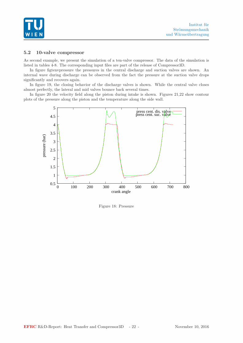
In figure figtenvpressure the pressures in the central discharge and suction valves are shown. Aninternal wave during discharge can be observed from the fact the pressure at the suction valve dropssignificantly and recovers again.

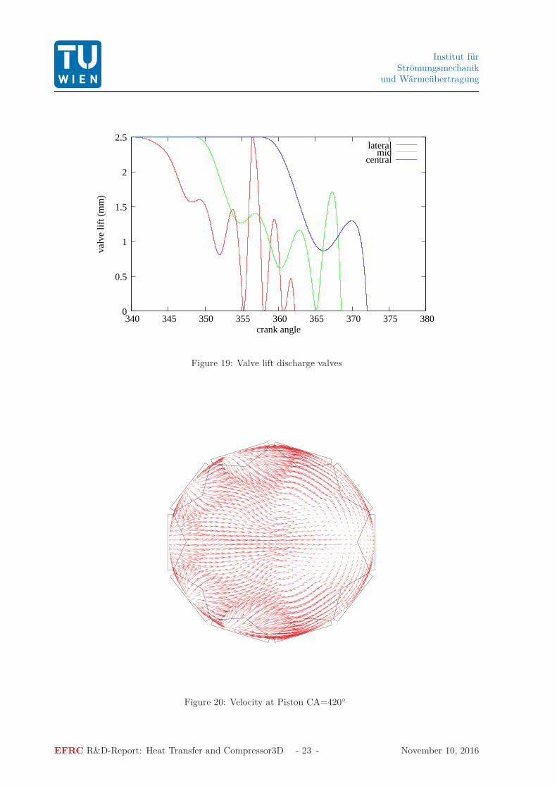
In figure 19, the closing behavior of the discharge valves is shown. While the central valve closesalmost perfectly, the lateral and mid valves bounce back several times.

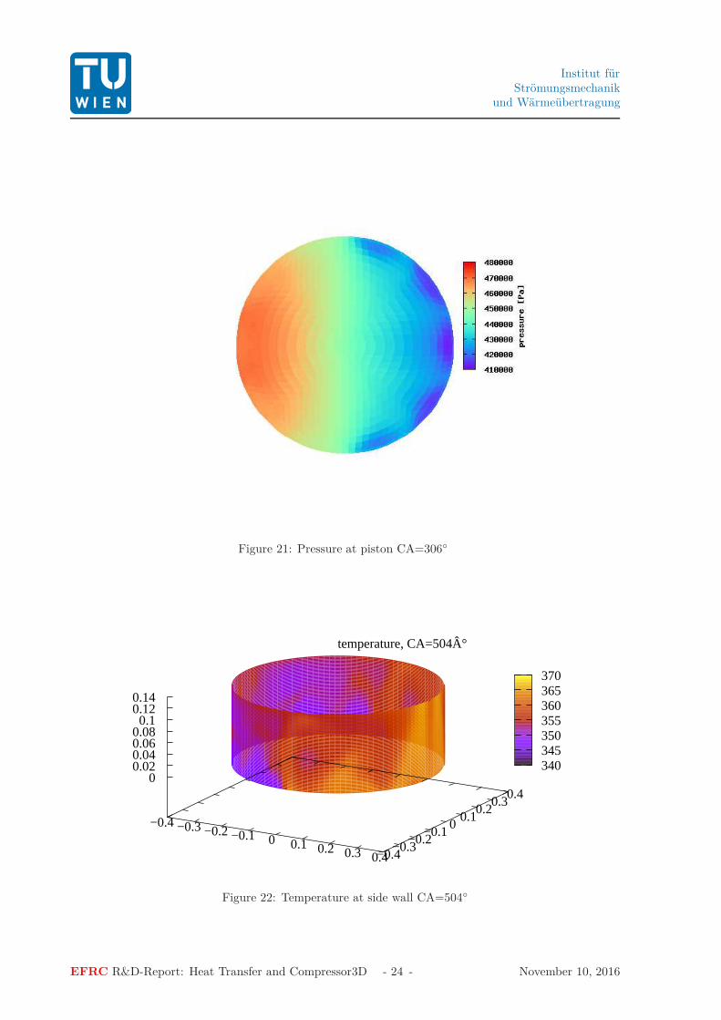
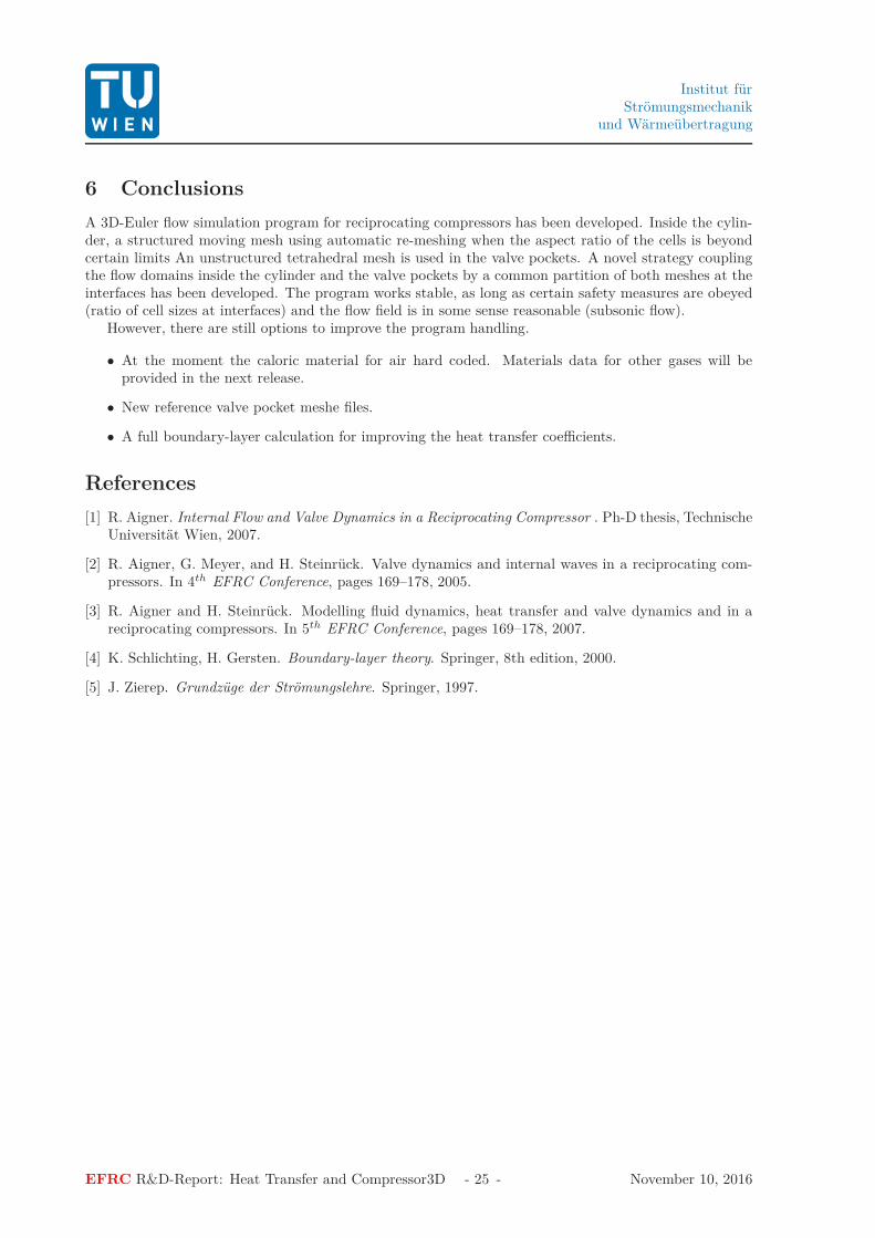
In figure 20 the velocity field along the piston during intake is shown. Figures 21,22 show contourplots of the pressure along the piston and the temperature along the side wall.

0.5

1

1.5

2

2.5

3

3.5

4

4.5

5

0 100 200 300 400 500 600 700 800

pres

sure

(ba

r)

crank angle

press cent. dis. valvepress cent. suc. valve

Figure 18: Pressure




0

0.5

1

1.5

2

2.5

340 345 350 355 360 365 370 375 380

valv

e lif

t (m

m)

crank angle

lateralmid

central

Figure 19: Valve lift discharge valves

Figure 20: Velocity at Piston CA=420◦




Figure 21: Pressure at piston CA=306◦

temperature, CA=504Â°

−0.4−0.3−0.2−0.1 0 0.1 0.2 0.3 0.4−0.4−0.3

−0.2−0.1

0 0.1

0.2 0.3

0.4 0

0.02 0.04 0.06 0.08 0.1

0.12 0.14

340 345 350 355 360 365 370

Figure 22: Temperature at side wall CA=504◦




6 Conclusions

A 3D-Euler flow simulation program for reciprocating compressors has been developed. Inside the cylin-der, a structured moving mesh using automatic re-meshing when the aspect ratio of the cells is beyondcertain limits An unstructured tetrahedral mesh is used in the valve pockets. A novel strategy couplingthe flow domains inside the cylinder and the valve pockets by a common partition of both meshes at theinterfaces has been developed. The program works stable, as long as certain safety measures are obeyed(ratio of cell sizes at interfaces) and the flow field is in some sense reasonable (subsonic flow).

However, there are still options to improve the program handling.

• At the moment the caloric material for air hard coded. Materials data for other gases will beprovided in the next release.

• New reference valve pocket meshe files.

• A full boundary-layer calculation for improving the heat transfer coefficients.

References

[1] R. Aigner. Internal Flow and Valve Dynamics in a Reciprocating Compressor . Ph-D thesis, TechnischeUniversität Wien, 2007.

[2] R. Aigner, G. Meyer, and H. Steinrück. Valve dynamics and internal waves in a reciprocating com-pressors. In 4th EFRC Conference, pages 169–178, 2005.

[3] R. Aigner and H. Steinrück. Modelling fluid dynamics, heat transfer and valve dynamics and in areciprocating compressors. In 5th EFRC Conference, pages 169–178, 2007.

[4] K. Schlichting, H. Gersten. Boundary-layer theory. Springer, 8th edition, 2000.

[5] J. Zierep. Grundzüge der Strömungslehre. Springer, 1997.


Heat Transfer in Reciprocating Compressors - Compressor3D Heat Transfer in Reciprocating Compressors...

Documents

Transcript of Heat Transfer in Reciprocating Compressors - Compressor3D Heat Transfer in Reciprocating Compressors...