Heat Transfer in Industrial...
526
HEAT T RANSFER IN INDUSTRIAL COMBUSTION Charles E. Baukal, Jr. Boca Raton New York CRC Press © 2000 by CRC Press LLC
Transcript of Heat Transfer in Industrial...

HEAT TRANSFER IN INDUSTRIAL COMBUSTION
Charles E. Baukal, Jr.
Boca Raton New York
CRC Press
© 2000 by CRC Press LLC

This book contains information obtained from authentic and highly regarded sources. Reprinted material is quoted with permission, and sources are indicated. A wide variety of references are listed. Reasonable efforts have been made to publish reliable data and information, but the author and the publisher cannot assume responsibility for the validity of all materials or for the consequences of their use.
Neither this book nor any part may be reproduced or transmitted in any form or by any means, electronic or mechanical, including photocopying, microfilming, and recording, or by any information storage or retrieval system, without prior permission in writing from the publisher.
All rights reserved. Authorization to photocopy items for internal or personal use, or the personal or internal use of specific clients, may be granted by CRC Press LLC, provided that $.50 per page photocopied is paid directly to Copyright Clearance Center, 222 Rosewood Drive, Danvers, MA 01923 USA. The fee code for users of the Transactional Reporting Service is ISBN 0-8493-1699-5/00/$0.00+$.50. The fee is subject to change without notice. For organizations that have been granted a photocopy license by the CCC, a separate system of payment has been arranged.
The consent of CRC Press LLC does not extend to copying for general distribution, for promotion, for creating new works, or for resale. Specific permission must be obtained in writing from CRC Press LLC for such copying.
Direct all inquiries to CRC Press LLC, 2000 N.W. Corporate Blvd., Boca Raton, Florida 33431.
Trademark Notice: Product or corporate names may be trademarks or registered trademarks, and are used only for identification and explanation, without intent to infringe.
© 2000 by CRC Press LLC
No claim to original U.S. Government worksInternational Standard Book Number 0-8493-1699-5
Library of Congress Card Number 99-088045Printed in the United States of America 1 2 3 4 5 6 7 8 9 0
Printed on acid-free paper
Library of Congress Cataloging-in-Publication DataBaukal, Charles E.
Heat transfer in industrial combustion / Charles E. Baukal, Jr.p. cm.
Includes bibliographical references and index.ISBN 0-8493-1699-5 (alk. paper)1. Heat--Transmission. 2. Combustion engineering. I. Title
TJ260.B359 2000621.402′2--dc21 99-088045
© 2000 by CRC Press LLC

Preface
This book is intended to fill a gap in the literature for books on heat transfer in industrial combustion, written primarily for the practicing engineer. Many textbooks have been written on both heat transfer and combustion, but both types of book generally have only a limited amount of information concerning the combination of heat transfer and industrial combustion. One of the purposes of this book is to codify the many relevant books, papers, and reports that have been written on this subject into a single, coherent reference source.
The key difference for this book compared to others is that it looks at each topic from a somewhat narrow scope to see how that topic affects heat transfer in industrial combustion. For example, in Chapter 2, the basics of combustion are considered, but from the limited perspective as to how combustion influences the heat transfer. There is very little discussion of combustion kinetics because in the overall combustion system, the kinetics of the chemical reactions in the flame only significantly impact the heat transfer in somewhat limited circumstances. Therefore, this book does not attempt to go over subjects that have been more than adequately covered in other books, but rather attempts to look at those subjects through the narrow lens of how they influence the heat transfer in the system.
The book is basically organized in three parts. The first part deals with the basics of heat transfer in combustion and includes chapters on the modes of heat transfer, computer modeling, and experimental techniques. The middle part of the book deals with general concepts of heat transfer in industrial combustion systems and includes chapters on heat transfer from flame impinge-ment, from burners, and in furnaces. The last part of the book deals with specific applications of heat transfer in industrial combustion and includes chapters on lower and higher temperature applications and some advanced applications. The book has discussions on the use of oxygen to enhance combustion and on flame impingement, both of particular interest to the author. These subjects have received very little, if any, coverage in previous books on heat transfer in industrial combustion.
As with any book of this type, there are many topics that are not covered. The book does not address other aspects of heat transfer in combustion such as power generation (stationary turbines or boilers) and propulsion (internal combustion, gas turbine or rocket engines), which are not normally considered to be industrial applications. It also does not treat packed bed combustion, material synthesis in flames, or flare applications, which are all fairly narrow in scope. Because the vast majority of industrial applications use gaseous fuels, that is the focus of this book, with only a cursory discussion of solid and liquid fuels. This book basically concerns atmospheric combustion, which is the predominant type used in industry. There are also many topics that are discussed in the book, but with a very limited treatment. One example is optical diagnostics. The reason for the limited discussion is that there has been very little application of such techniques to industrial combustors because of the difficulties in making them work on a large scale in sometimes hostile environments.
This book attempts to focus on those topics that are of interest to the practicing engineer. It does not profess to be exhaustively comprehensive, but does attempt to provide references for the interested reader who would like more information on a particular subject. As most authors know, it is always a struggle about what to include and what not to include in a book. Here, the guideline that has been used is to minimize the theory and maximize the applications, while at the same time trying to at least touch on the relevant topics for heat transfer in industrial combustion.
© 2000 by CRC Press LLC

About the Author
Charles E. Baukal, Jr., Ph.D., P.E., is the Director of the John Zink Company LLC R & D Test Center in Tulsa, OK. He has 20 years of experience in the fields of heat transfer and industrial combustion and has authored more than 50 publications in those fields, including editing the book Oxygen-Enhanced Combustion (CRC Press, Boca Raton, FL, 1998). He has a Ph.D. in mechanical engineering from the University of Pennsylvania, is a licensed Professional Engineer in the state of Pennsylvania, has been an adjunct instructor at several colleges, and has eight U.S. patents.
© 2000 by CRC Press LLC
Acknowledgment
This book is dedicated to my wife Beth, to my children Christine, Caitlyn, and Courtney, and to my mother Elaine. This book is also dedicated to the memories of my father, Charles, Sr. and my brother, Jim, who have both gone on to be with their maker.
The author would like to thank Tom Smith of Marsden, Inc. (Pennsauken, NJ) and Buddy Eleazer of Air Products (Allentown, PA) for the opportunities to learn firsthand about heat transfer in industrial combustion. The author would also like to thank David Koch and Dr. Roberto Ruiz of John Zink Company LLC (Tulsa, OK) for their support in the writing of this book. Last but not least, the author would like to thank the good Lord above, without whom this would not have been possible.
Charles E. Baukal, Jr., Ph.D., P.E.
© 2000 by CRC Press LLC

NomenclatureSymbol Description Units
A Area ft2 or m2
c Speed of light ft/sec or m/seccp Specific heat Btu/lb-°F or J/kg-KCp Pitot-Static probe calibration constant dimensionlessd Diameter in. or mmD Dimensionless diameter = d/dn dimensionlessDa Damköhler number (see Eq. 2.19) dimensionlesse Hemispherical emissive power Btu/hr-ft2 or kW/m2
E Error dimensionlessE Hemispherical emissive power Btu/hr or kWF1-2 Radiation view factor from surface 1 to surface 2 dimensionlessGr Grashoff number (see Eq. 3.12) dimensionlessh Convection heat transfer coefficient Btu/hr-ft2-°F or W/m2-KhC Chemical enthalpy Btu/lb or J/kghfusion Heat of fusion Btu/lb or J/kghS Sensible enthalpy = ½cpdt Btu/lb or J/kghT Total enthalpy = hC + hS Btu/lb or J/kgH Fuel heat content Btu/lb or kJ/kgI Radiation intensity Btu/hr-ft2-µm or W/m2-µmk Thermal conductivity Btu/hr-ft-°F or W/m-KK Non-absorption factor for radiation dimensionlessKa Absorption coefficient for radiation dimensionlessKs Scattering coefficient for radiation dimensionlessl Length in. or mmlv Potential core length for velocity in. or mmL Distance between the burner and the target = lj/dn dimensionlessL Radiation path length through a gas ft or mLm Mean beam length ft or mLe Lewis number = ρcpDi–mix/k dimensionlessm• Mass flow rate lb/hr or kg/hrMa Mach number = v/c dimensionlessMW Molecular weight lb/lb-mole or g/g-moleNu Nusselt number (see Eq. 3.3) dimensionlesspst Static pressure psig or Papt Total pressure psig or PaPr Prandtl number = cpµ/k (see Eq. 3.2) dimensionlessq Heat flow Btu/hr or kWq″ Heat flux Btu/hr-ft2 or kW/m2
qf Burner firing rate Btu/hr or kWqi Heat absorbed by calorimeter i Btu/hr or kWQ Gas flow rate ft3/hr or m3/hrr Radial distance from the burner centerline in. or mmR Dimensionless radius = r/dn dimensionlessRa Rayleigh number (see Eq. 3.11) dimensionlessRe Reynolds number = ρvd/µ (see Eq. 3.1) dimensionlessRi Richardson number (see Eq. 3.13) dimensionlessS Stoichiometry (see Eqs. 2.3 and 2.5) dimensionless
© 2000 by CRC Press LLC

SL Laminar flame speed ft/s or m/st Temperature °F or K
T Absolute temperature °R or KTu Turbulence intensity dimensionlessv Velocity ft/s or m/sV Volume ft3 or m3
x Axial distance from the burner to the target stagnation point in. or mmX Distance from the burner to the target stagnation point = x/dn dimensionlessXv Potential core length for velocity = lv/dn dimensionless
Greek Symbolsα Absorptivity dimensionlessβ Velocity gradient s–1
β~
Volume coefficient of expansion °R–1 or K–1
δ Boundary layer thickness in. or mmε Emissivity dimensionlessη Thermal efficiency dimensionless Absorption coefficient of a luminous gas ft–1 or m–1
µ Absolute or dynamic viscosity lb/ft-s or kg/m-sγ Turbulence enhancement factor (see Eq. 7.25) dimensionless
Ω Oxidizer composition = dimensionless
φ Equivalence ratio = dimensionless
δ Soot radiation index (see Eq. 3.53) dimensionlessλ Fuel mixture ratio (see Eq. 2.8) dimensionlessλ Wavelength µmν Frequency s–1
ν Kinematic viscosity ft2/s or m2/sρ Density lb/ft3 or kg/m3
ρ Reflectivity dimensionlessσ Stefan-Boltzmann constant Btu/hr-ft2-°R4 or W/m2-K4
Φ Surface catalytic efficiency (see Eq. 7.26) dimensionlessθradm Radiometer field of view degreesτ Optical density sτ Transmissivity dimensionlessτ Time s
O
N2
2
volume in the oxidizer
O volume in the oxidizer2 +
Stoichiometric oxygen Fuel volume ratioActual oxygen Fuel volume ratio
Subscriptsb Stagnation body or target n Burner nozzleconv Convective heat transfer NG Natural gase Edge of boundary layer p Probeeff Effective diameter r Radial directionf Fluid rad Thermal radiationf Film temperature (see Eq. 4.7) radm Radiometerg Gas rec Recovery temperature (see Eq. 7.6)× Ambient conditions ref Reference temperature (see Eq. 7.5)j Jet s Stagnation pointj Thermocouple junction T Turbulentl Load T/C ThermocoupleK Kolmogorov w Wall (target surface)m Medium υ Volumetricmax Maximum
© 2000 by CRC Press LLC

Table of Contents
Chapter 1 Introduction1.1 Importance of Heat Transfer in Industrial Combustion
1.1.1 Energy Consumption1.1.2 Research Needs
1.2 Literature Discussion1.2.1 Heat Transfer1.2.2 Combustion1.2.3 Heat Transfer and Combustion
1.3 Combustion System Components1.3.1 Burners
1.3.1.1 Competing Priorities1.3.1.2 Design Factors
1.3.1.2.1 Fuel1.3.1.2.2 Oxidizer1.3.1.2.3 Gas Recirculation
1.3.1.3 General Burner Types1.3.1.3.1 Mixing Type1.3.1.3.2 Oxidizer Type1.3.1.3.3 Draft Type1.3.1.3.4 Heating Type
1.3.2 Combustors1.3.2.1 Design Considerations
1.3.2.1.1 Load Handling1.3.2.1.2 Temperature1.3.2.1.3 Heat Recovery
1.3.2.2 General Classifications1.3.2.2.1 Load Processing Method1.3.2.2.2 Heating Type1.3.2.2.3 Geometry1.3.2.2.4 Heat Recuperation
1.3.3 Heat Load1.3.3.1 Process Tubes1.3.3.2 Moving Substrate1.3.3.3 Opaque Materials1.3.3.4 Transparent Materials
1.3.4 Heat Recovery Devices1.3.4.1 Recuperators1.3.4.2 Regenerators
References
Chapter 2 Some Fundamentals of Combustion2.1 Combustion Chemistry
2.1.1 Fuel Properties2.1.2 Oxidizer Composition
© 2000 by CRC Press LLC

2.1.3 Mixture Ratio2.1.4 Operating Regimes
2.2 Combustion Properties
2.2.1 Combustion Products2.2.1.1 Oxidizer Composition2.2.1.2 Mixture Ratio2.2.1.3 Air and Fuel Preheat Temperature2.2.1.4 Fuel Composition
2.2.2 Flame Temperature2.2.2.1 Oxidizer and Fuel Composition2.2.2.2 Mixture Ratio2.2.2.3 Oxidizer and Fuel Preheat Temperature
2.2.3 Available Heat2.2.4 Flue Gas Volume
2.3 Exhaust Product Transport Properties2.3.1 Density2.3.2 Specific Heat2.3.3 Thermal Conductivity2.3.4 Viscosity2.3.5 Prandtl Number2.3.6 Lewis Number
References
Chapter 3 Heat Transfer Modes3.1 Introduction3.2 Convection
3.2.1 Forced Convection3.2.1.1 Forced Convection from Flames3.2.1.2 Forced Convection from Outside Combustor Wall3.2.1.3 Forced Convection from Hot Gases to Tubes
3.2.2 Natural Convection3.2.2.1 Natural Convection from Flames3.2.2.2 Natural Convection from Outside Combustor Wall
3.3 Radiation3.3.1 Surface Radiation3.3.2 Nonluminous Radiation
3.3.2.1 Theory3.3.2.2 Combustion Studies
3.3.2.2.1 Total Radiation3.3.2.2.2 Spectral Radiation
3.3.3 Luminous Radiation3.3.3.1 Theory3.3.3.2 Combustion Studies
3.3.3.2.1 Total Radiation3.3.3.2.2 Spectral Radiation
3.4 Conduction3.4.1 Steady-State Conduction3.4.2 Transient Conduction
3.5 Phase Change3.5.1 Melting3.5.2 Boiling
© 2000 by CRC Press LLC
3.5.2.1 Internal Boiling3.5.2.2 External Boiling
3.5.3 Condensation
References
Chapter 4 Heat Sources and Sinks4.1 Heat Sources
4.1.1 Combustibles4.1.1.1 Fuel Combustion4.1.1.2 Volatile Combustion
4.1.2 Thermochemical Heat Release4.1.2.1 Equilibrium TCHR4.1.2.2 Catalytic TCHR4.1.2.3 Mixed TCHR
4.2 Heat Sinks4.2.1 Load
4.2.1.1 Tubes4.2.1.2 Substrate4.2.1.3 Granular Solid4.2.1.4 Molten Liquid4.2.1.5 Surface Conditions
4.2.1.5.1 Radiation4.2.1.5.2 Catalyticity
4.2.2 Wall Losses4.2.3 Openings
4.2.3.1 Radiation4.2.3.2 Gas Flow Through Openings
4.2.4 Material TransportReferences
Chapter 5 Computer Modeling5.1 Combustion Modeling5.2 Modeling Approaches
5.2.1 Fluid Dynamics5.2.1.1 Moment Averaging5.2.1.2 Vortex Methods5.2.1.3 Spectral Methods5.2.1.4 Direct Numerical Simulation
5.2.2 Geometry5.2.2.1 Zero-Dimensional Modeling5.2.2.2 One-Dimensional Modeling5.2.2.3 Multi-dimensional Modeling
5.2.3 Reaction Chemistry5.2.3.1 Nonreacting Flows5.2.3.2 Simplified Chemistry5.2.3.3 Complex Chemistry
5.2.4 Radiation5.2.4.1 Nonradiating5.2.4.2 Participating Media
5.2.5 Time Dependence
© 2000 by CRC Press LLC

5.2.5.1 Steady State5.2.5.2 Transient
5.3 Simplified Models5.4 Computational Fluid Dynamic Modeling
5.4.1 Increasing Popularity of CFD5.4.2 Potential Problems of CFD5.4.3 Equations
5.4.3.1 Fluid Dynamics5.4.3.2 Heat Transfer5.4.3.3 Chemistry5.4.3.4 Multiple Phases
5.4.4 Boundary and Initial Conditions5.4.4.1 Inlets and Outlets5.4.4.2 Surfaces5.4.4.3 Symmetry
5.4.5 Discretization5.4.5.1 Finite Difference Technique5.4.5.2 Finite Volume Technique5.4.5.3 Finite Element Technique5.4.5.4 Mixed5.4.5.5 None
5.4.6 Solution Methods5.4.7 Model Validation5.4.8 Industrial Combustion Examples
5.4.8.1 Modeling Burners5.4.8.2 Modeling Combustors
References
Chapter 6 Experimental Techniques6.1 Introduction6.2 Heat Flux
6.2.1 Total Heat Flux6.2.1.1 Steady-State Uncooled Solids6.2.1.2 Steady-State Cooled Solids
6.2.1.2.1 Single Cooling Circuit6.2.1.2.2 Multiple Cooling Circuits6.2.1.2.3 Surface Probe
6.2.1.3 Steady-State Cooled Gages6.2.1.3.1 Gradient Through a Thin Solid Rod6.2.1.3.2 Thin Disk Calorimeter6.2.1.3.3 Heat Flux Transducer
6.2.1.4 Transient Uncooled Targets6.2.1.5 Transient Uncooled Gages
6.2.1.5.1 Slug Calorimeter6.2.1.5.2 Heat Flux Transducer
6.2.2 Radiant Heat Flux6.2.2.1 Heat Flux Gage6.2.2.2 Ellipsoidal Radiometer6.2.2.3 Spectral Radiometer6.2.2.4 Other Techniques
6.2.3 Convective Heat Flux
© 2000 by CRC Press LLC
6.3 Temperature6.3.1 Gas Temperature
6.3.1.1 Suction Pyrometer6.3.1.2 Optical Techniques6.3.1.3 Fine Wire Thermocouples6.3.1.4 Line Reversal
6.3.2 Surface Temperature6.3.2.1 Embedded Thermocouple6.3.2.2 Infrared Detectors
6.4 Gas Flow6.4.1 Gas Velocity
6.4.1.1 Pitot Tubes6.4.1.2 Laser Doppler Velocimetry6.4.1.3 Other Techniques
6.4.2 Static Pressure Distribution6.4.2.1 Stagnation Velocity Gradient6.4.2.2 Stagnation Zone
6.5 Gas Species6.6 Other Measurements6.7 Physical ModelingReferences
Chapter 7 Flame Impingement7.1 Introduction7.2 Experimental Conditions
7.2.1 Configurations7.2.1.1 Flame Normal to a Cylinder in Crossflow7.2.1.2 Flame Normal to a Hemispherically Nosed Cylinder7.2.1.3 Flame Normal to a Plane Surface7.2.1.4 Flame Parallel to a Plane Surface
7.2.2 Operating Conditions7.2.2.1 Oxidizers7.2.2.2 Fuels7.2.2.3 Equivalence Ratios7.2.2.4 Firing Rates7.2.2.5 Reynolds Number7.2.2.6 Burners7.2.2.7 Nozzle Diameter7.2.2.8 Location
7.2.3 Stagnation Targets7.2.3.1 Size7.2.3.2 Target Materials7.2.3.3 Surface Preparation7.2.3.4 Surface Temperatures
7.2.4 Measurements7.3 Semianalytical Heat Transfer Solutions
7.3.1 Equation Parameters7.3.1.1 Thermophysical Properties7.3.1.2 Stagnation Velocity Gradient
7.3.1.2.1 Analytical Solutions7.3.1.2.2 Empirical Correlations
© 2000 by CRC Press LLC

7.3.2 Equations7.3.2.1 Sibulkin Results
7.3.2.2 Fay and Riddell Results7.3.2.3 Rosner Results
7.3.3 Comparisons With Experiments7.3.3.1 Forced Convection (Negligible TCHR)
7.3.3.1.1 Laminar Flow7.3.3.1.2 Turbulent Flows
7.3.3.2 Forced Convection with TCHR7.3.3.2.1 Laminar Flow7.3.3.2.2 Turbulent Flow
7.3.4 Sample Calculations7.3.4.1 Laminar Flames Without TCHR7.3.4.2 Turbulent Flames Without TCHR7.3.4.3 Laminar Flames with TCHR
7.3.5 Summary7.4 Empirical Heat Transfer Correlations
7.4.1 Thermophysical Properties7.4.2 Flames Impinging Normal to a Cylinder
7.4.2.1 Local Convection Heat Transfer7.4.2.1.1 Laminar and Turbulent Flows7.4.2.1.2 Turbulent Flows
7.4.2.2 Average Convection Heat Transfer7.4.2.2.1 Laminar Flows7.4.2.2.2 Laminar and Turbulent Flows7.4.2.2.3 Flow Type Unspecified
7.4.2.3 Average Convection Heat Transfer with TCHR7.4.2.3.1 Flow Type Unspecified
7.4.2.4 Average Radiation Heat Transfer7.4.2.4.1 Laminar and Turbulent Flows
7.4.2.5 Maximum Convection and Radiation Heat Transfer7.4.2.5.1 Turbulent Flows
7.4.3 Flames Impinging Normal to a Hemi-Nosed Cylinder7.4.3.1 Local Convection Heat Transfer
7.4.3.1.1 Laminar and Turbulent Flows7.4.3.1.2 Turbulent Flows
7.4.3.2 Local Convection Heat Transfer with TCHR7.4.3.2.1 Turbulent Flows
7.4.4 Flames Impinging Normal to a Plane Surface7.4.4.1 Local Convection Heat Transfer
7.4.4.1.1 Laminar Flows7.4.4.1.2 Turbulent Flows
7.4.4.2 Local Convection Heat Transfer with TCHR7.4.4.2.1 Laminar Flows7.4.4.2.2 Turbulent Flows
7.4.4.3 Average Convection Heat Transfer7.4.4.3.1 Laminar Flows7.4.4.3.2 Turbulent Flows
7.4.5 Flames Parallel to a Plane Surface7.4.5.1 Local Convection Heat Transfer With TCHR
© 2000 by CRC Press LLC
7.4.5.1.1 Laminar Flows7.4.5.1.2 Turbulent Flows
7.4.5.2 Local Convection and Radiation Heat Transfer
7.4.5.2.1 Turbulent FlowsReferences
Chapter 8 Heat Transfer from Burners8.1 Introduction8.2 Open-Flame Burners
8.2.1 Momentum Effects8.2.2 Flame Luminosity8.2.3 Firing Rate Effects8.2.4 Flame Shape Effects
8.3 Radiant Burners8.3.1 Perforated Ceramic or Wire Mesh Radiant Burners8.3.2 Flame Impingement Radiant Burners8.3.3 Porous Refractory Radiant Burners8.3.4 Advanced Ceramic Radiant Burners8.3.5 Radiant Wall Burners8.3.6 Radiant Tube Burners
8.4 Effects on Heat Transfer8.4.1 Fuel Effects
8.4.1.1 Solid Fuels8.4.1.2 Liquid Fuels8.4.1.3 Gaseous Fuels8.4.1.4 Fuel Temperature
8.4.2 Oxidizer Effects8.4.2.1 Oxidizer Composition8.4.2.2 Oxidizer Temperature
8.4.3 Staging Effects8.4.3.1 Fuel Staging8.4.3.2 Oxidizer Staging
8.4.4 Burner Orientation8.4.4.1 Hearth-Fired Burners8.4.4.2 Wall-Fired Burners8.4.4.3 Roof-Fired Burners8.4.4.4 Side-Fired Burners
8.4.5 Heat Recuperation8.4.5.1 Regenerative Burners8.4.5.2 Recuperative Burners8.4.5.3 Furnace or Flue Gas Recirculation
8.4.6 Pulse Combustion8.5 In-Flame TreatmentReferences
Chapter 9 Heat Transfer in Furnaces9.1 Introduction9.2 Furnaces
9.2.1 Firing Method
© 2000 by CRC Press LLC
9.2.1.1 Direct Firing9.2.1.2 Indirect Firing
9.2.1.3 Heat Distribution
9.2.2 Load Processing Method9.2.2.1 Batch Processing9.2.2.2 Continuous Processing9.2.2.3 Hybrid Processing
9.2.3 Heat Transfer Medium9.2.3.1 Gaseous Medium9.2.3.2 Vacuum9.2.3.3 Liquid Medium9.2.3.4 Solid Medium
9.2.4 Geometry9.2.4.1 Rotary Geometry9.2.4.2 Rectangular Geometry9.2.4.3 Ladle Geometry9.2.4.4 Vertical Cylindrical Geometry
9.2.5 Furnace Types9.2.5.1 Reverberatory Furnace9.2.5.2 Shaft Kiln9.2.5.3 Rotary Furnace
9.3 Heat Recovery9.3.1 Recuperators9.3.2 Regenerators9.3.3 Gas Recirculation
9.3.3.1 Flue Gas Recirculation9.3.3.2 Furnace Gas Recirculation
References
Chapter 10 Lower Temperature Applications10.1 Introduction10.2 Ovens and Dryers
10.2.1 Predryer10.2.2 Dryer
10.3 Fired Heaters10.3.1 Reformer10.3.2 Process Heater
10.4 Heat Treating10.4.1 Standard Atmosphere10.4.2 Special Atmosphere
References
Chapter 11 Higher Temperature Applications11.1 Introduction
11.1.1 Furnaces11.1.2 Industries
11.2 Metals Industry11.2.1 Ferrous Metal Production
11.2.1.1 Electric Arc Furnace11.2.1.2 Smelting
© 2000 by CRC Press LLC

11.2.1.3 Ladle Preheating11.2.1.4 Reheating Furnace
11.2.1.5 Forging
11.2.2 Aluminum Metal Production11.3 Minerals Industry
11.3.1 Glass11.3.1.1 Types of Traditional Glass-Melting Furnaces11.3.1.2 Unit Melter11.3.1.3 Recuperative Melter11.3.1.4 Regenerative or Siemens Furnace
11.3.1.4.1 End-Port Regenerative Furnace11.3.1.4.2 Side-Port Regenerative Furnace
11.3.1.5 Oxygen-Enhanced Combustion for Glass Production11.3.1.6 Advanced Techniques for Glass Production
11.3.2 Cement and Lime11.3.3 Bricks, Refractories, and Ceramics
11.4 Waste Incineration11.4.1 Types of Incinerators
11.4.1.1 Municipal Waste Incinerators11.4.1.2 Sludge Incinerators11.4.1.3 Mobile Incinerators11.4.1.4 Transportable Incinerators11.4.1.5 Fixed Hazardous Waste Incinerators
11.4.2 Heat Transfer in Waste IncinerationReferences
Chapter 12 Advanced Combustion Systems12.1 Introduction12.2 Oxygen-Enhanced Combustion
12.2.1 Typical Use Methods12.2.1.1 Air Enrichment12.2.1.2 O2 Lancing12.2.1.3 Oxy/Fuel12.2.1.4 Air-Oxy/Fuel
12.2.2 Operating Regimes12.2.3 Heat Transfer Benefits
12.2.3.1 Increased Productivity12.2.3.2 Higher Thermal Efficiencies12.2.3.3 Higher Heat Transfer Efficiency12.2.3.4 Increased Flexibility
12.2.4 Potential Heat Transfer Problems12.2.4.1 Refractory Damage12.2.4.2 Nonuniform Heating
12.2.4.2.1 Hotspots12.2.4.2.2 Reduction in Convection
12.2.5 Industrial Heating Applications12.2.5.1 Metals12.2.5.2 Minerals12.2.5.3 Incineration12.2.5.4 Other
© 2000 by CRC Press LLC

12.3 Submerged Combustion12.3.1 Metals Production
12.3.2 Minerals Production12.3.3 Liquid Heating
12.4 Miscellaneous12.4.1 Surface Combustor-Heater12.4.2 Direct-Fired Cylinder Dryer
References
AppendicesAppendix A: Reference Sources for Further InformationAppendix B: Common ConversionsAppendix C: Methods of Expressing Mixture Ratios for CH4, C3H8, and H2
Appendix D: Properties for CH4, C3H8, and H2 FlamesAppendix E: Fluid Dynamics EquationsAppendix F: Material Properties
© 2000 by CRC Press LLC

Introduction
11.1 IMPORTANCE OF HEAT TRANSFER IN INDUSTRIAL
COMBUSTION
This chapter section briefly attempts to establish the importance of heat transfer in industrial combustion by first looking at how much energy is consumed by industry and then by the number of recommendations for continued research into heat transfer for industrial combustion applications.
1.1.1 ENERGY CONSUMPTION
Industry relies heavily on the combustion process as shown in Table 1.1. The major uses for combustion in industry are shown in Table 1.2. Hewitt et al. (1994) have listed some of the common heating applications used in industry, as shown in Table 1.3.1 Typical industrial combustion appli-cations can also be characterized by their temperature ranges, as shown in Figure 1.1. As can be seen in Figure 1.2, the demand for energy is expected to continue to rapidly increase. Most of the energy (88%) is produced by the combustion of fossil fuels like oil, natural gas, and coal. According to the U.S. Department of Energy, the demand in the industrial sector is projected to increase by 0.8% per year to the year 2020.2
The objective in nearly all industrial combustion applications is to transfer that energy to some type of load for thermal processing of that load.3 Examples of the many types of thermal processes include heating solids to the softening point for forming, drying for moisture removal, and chemical processing in calcining. Depending on the application, the heat may be transferred directly from the flame to the load, or indirectly from the flame to a heat transfer medium like a ceramic tube. The sheer amount of energy used by industry makes heat transfer in industrial combustion an important subject.
1.1.2 RESEARCH NEEDS
Many studies have recommended further research into heat transfer in industrial combustion for a wide range of reasons. One obvious reason includes increasing fuel efficiency in the light of the substantial energy consumption in industry in the combustion of fossil fuels. Another reason is to optimize existing processes to increase throughput or productivity for a given size combustion system. Further research is needed to develop new processes as new materials and products need to be heated during processing. Research is needed in both the computer simulation of the com-bustion processes and in making experimental measurements in those processes.
Knowles (1986) described future combustion systems using natural gas.4 The systems involving both combustion and heat transfer included higher temperature air preheaters and higher heat flux furnaces. Pohl et al. (1986) gave 15 recommendations for research to improve energy efficiency in the process industries.5 The major ones that included heat transfer were:
• Furnace design, heat and mixing patterns• Heat recovery and energy efficiency of flares• Recuperative burner for low heating value gases• Impinging (pulsed) heat transfer• Rich flames for higher thermal radiation
© 2000 by CRC Press LLC

TABLE 1.1
The Importance of Combustion to Industry
% Total Energy from (at the point of use)
Industry Steam Heat Combustion
Petroleum refining 29.6 62.6 92.2Forest products 84.4 6.0 90.4Steel 22.6 67.0 89.6Chemicals 49.9 32.7 82.6Glass 4.8 75.2 80.0Metal casting 2.4 67.2 69.6Aluminum 1.3 17.6 18.9
Source: From U.S. Dept. of Energy, Energy Information Administra-tion as quoted in the Industrial Combustion Vision, prepared by the U.S. Dept. of Energy, May 1998.
TABLE 1.2Major Process Heating Operations
Metal melting Bonding • Steel making • Sintering, brazing • Iron and steel melting Drying • Nonferrous melting • Surface film dryingMetal heating • Rubber, plastic, wood, glass products drying • Steel soaking, reheat, ladle preheating • Coal drying • Forging • Food processing • Nonferrous heating • Animal food processingMetal heat treating Calcining • Annealing • Cement, lime, soda ash • Stress relief • Alumina, gypsum • Tempering Clay firing • Solution heat treating • Structural products • Aging • Refractories • Precipitation hardening AgglomerationCuring and forming • Iron, lead, zinc • Glass annealing, tempering, forming Smelting • Plastics fabrication • Iron, copper, lead • Gypsum production Non-metallic materials meltingFluid heating • Glass • Oil and natural gas production Other heating • Chemical/petroleum feedstock preheating • Ore roasting • Distillation, visbreaking, hydrotreating, hydrocracking,
delayed coking • Textile manufacturing • Food production • Aluminum anode baking
Source: From Industrial Combustion Vision, U.S. Dept. of Energy, May 1998.
© 2000 by CRC Press LLC
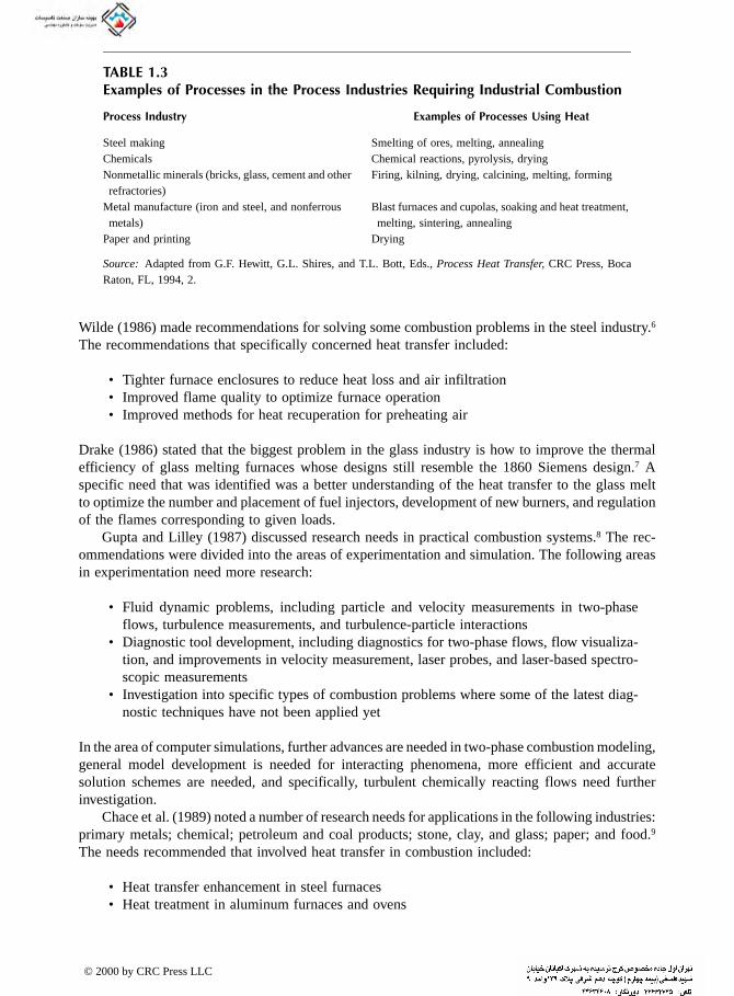
TABLE 1.3
Wilde (1986) made recommendations for solving some combustion problems in the steel industry.6
The recommendations that specifically concerned heat transfer included:
• Tighter furnace enclosures to reduce heat loss and air infiltration• Improved flame quality to optimize furnace operation• Improved methods for heat recuperation for preheating air
Drake (1986) stated that the biggest problem in the glass industry is how to improve the thermal efficiency of glass melting furnaces whose designs still resemble the 1860 Siemens design.7 A specific need that was identified was a better understanding of the heat transfer to the glass melt to optimize the number and placement of fuel injectors, development of new burners, and regulation of the flames corresponding to given loads.
Gupta and Lilley (1987) discussed research needs in practical combustion systems.8 The rec-ommendations were divided into the areas of experimentation and simulation. The following areas in experimentation need more research:
• Fluid dynamic problems, including particle and velocity measurements in two-phase flows, turbulence measurements, and turbulence-particle interactions
• Diagnostic tool development, including diagnostics for two-phase flows, flow visualiza-tion, and improvements in velocity measurement, laser probes, and laser-based spectro-scopic measurements
• Investigation into specific types of combustion problems where some of the latest diag-nostic techniques have not been applied yet
In the area of computer simulations, further advances are needed in two-phase combustion modeling, general model development is needed for interacting phenomena, more efficient and accurate solution schemes are needed, and specifically, turbulent chemically reacting flows need further investigation.
Chace et al. (1989) noted a number of research needs for applications in the following industries: primary metals; chemical; petroleum and coal products; stone, clay, and glass; paper; and food.9
The needs recommended that involved heat transfer in combustion included:
• Heat transfer enhancement in steel furnaces• Heat treatment in aluminum furnaces and ovens
Examples of Processes in the Process Industries Requiring Industrial Combustion
Process Industry Examples of Processes Using Heat
Steel making Smelting of ores, melting, annealingChemicals Chemical reactions, pyrolysis, dryingNonmetallic minerals (bricks, glass, cement and other
refractories)Firing, kilning, drying, calcining, melting, forming
Metal manufacture (iron and steel, and nonferrous metals)
Blast furnaces and cupolas, soaking and heat treatment, melting, sintering, annealing
Paper and printing Drying
Source: Adapted from G.F. Hewitt, G.L. Shires, and T.L. Bott, Eds., Process Heat Transfer, CRC Press, Boca Raton, FL, 1994, 2.
© 2000 by CRC Press LLC

hm, 1998. With permission.)
FIGURE 1.1 Temperature ranges of common industrial combustion applications. (Courtesy of Werner Da
© 2000 by CRC Press LLC

• Enhanced heat transfer in glass furnaces• Heat transfer enhancement in the chemical industry• Fluidized-bed heating system for the petroleum industry• Enhanced heat transfer rates in thermal processing in the chemical industry• Enhanced heat transfer in the pulp and paper industry• Accelerated drying in the food industry
Viskanta (1991) discussed some selected techniques for enhancing the heat transfer in fossil-fuel-fired industrial furnaces.10 Such improvements could lead to higher productivity and efficiency and, in some cases, reduced equipment size. Further research was recommended to improve models for radiative transfer in industrial furnaces that have fluctuating temperature and concentrations fields.
A study by the U.S. Department of Energy (DOE) identified many research opportunities involving heat transfer in industrial combustion.11 In the petroleum refining industry, high-temper-ature furnace efficiency improvements through flame radiation enhancement were recommended. Some recommendations were given for steel industry research, specifically in reheat furnaces: improve the uniformity of the generation and application of heat to the steel and conduct funda-mental flame research to verify the actual heat transfer achieved by various types of burners. For the metal casting industry, improvements were recommended for waste heat recovery and for general heat transfer in the heating process. Development of enhanced heat transfer mechanisms was recommended for the chemical industry. Optimizing the heat transfer to molten glass, improving waste heat recovery, and improving computer models of the heating and melting process were recommended as research needs in the glass industry. In the aluminum industry, furnace efficiency and productivity improvements through flame radiation for secondary aluminum melters and treat-ing furnaces were recommended. Improved computer models were recommended for simulating the black liquor combustion process in the pulp and paper industry.
Kurek et al. (1998) noted that recent research in industrial combustion has been directed at improving the energy utilization in the process industries.12 Five general areas of research were listed and three of those concern improving heat transfer in some way: (1) improving process productivity (increasing heat flux rates), (2) improving process temperature uniformity (improving
FIGURE 1.2 Historical and projected world energy consumption. (U.S. Dept. of Energy, Energy Information Administration, Annual Energy Outlook 1999, Report DOE/EIA-0383(99) Washington, D.C.)
© 2000 by CRC Press LLC

the heat flux distribution), and (3) improving thermal efficiency (improving the energy transfer from the heat source to the load).
The U.S. DOE developed a “technology roadmap” for industrial combustion with the help of
representatives from users and manufacturers in industry and from academia.13 A number of research needs in industrial combustion, directly or indirectly concerning heat transfer, were identified:
• New furnace designs (heat transfer needed for the analysis)• Cost-effective heat recovery processes• Optimization of the emissivity of materials used in furnaces or burners• Increased combustion intensity (heat release per unit of furnace volume)• Adaptation of computational fluid dynamics models to design burners• Development of new equipment and methods for heating and transferring heat• Development of hybrid or other methods to increase heat transfer to loads
1.2 LITERATURE DISCUSSION
The subject of this book is heat transfer — specifically in industrial combustion systems. This chapter section briefly considers some of the relevant literature on the subjects of heat transfer, combustion, and the combination of combustion with heat transfer. Many textbooks have been written on both heat transfer and combustion, but both types of book generally have only a limited amount of information concerning the combination of heat transfer and industrial combustion. Most of these books were written at a highly technical level for use in upper-level undergraduate or graduate-level courses. The books typically have broad coverage, with less emphasis on practical applications due to the nature of their target audience. This chapter section briefly surveys books related to heat transfer, combustion, and heat transfer in combustion. A list of relevant journals and trade magazines on this subject is given in Appendix A.
1.2.1 HEAT TRANSFER
Numerous excellent books have been written on the subject of heat transfer. However, almost none of them have any significant discussion of combustion. This is not surprising as the field of heat transfer is very broad, which makes it very difficult to be exhaustively comprehensive. Many of the heat transfer textbooks have no specific discussion of heat transfer in industrial combustion but do treat gaseous radiation heat transfer.14-19,19a
The heat transfer books written specifically about radiation often have sections covering heat transfer from luminous and nonluminous flames. Those topics are also discussed in this book in Chapter 4. Hottel and Sarofim’s (1967) book has a good blend of theory and practice regarding radiation.20 It also has a chapter specifically devoted to applications in furnaces. Love’s (1968) book on radiation has short theoretical discussions of radiative heat transfer in flames and measuring flame parameters, but no other significant discussions of flames and combustion.21 Özisik’s (1973) book focuses more on interactions between radiation and conduction and convection, with no specific treatment of combustion or flames.22 A short book by Gray and Müller (1974) is aimed toward more practical applications of radiation.23 Sparrow and Cess (1978) have a brief chapter on nonluminous gaseous radiation, in which the various band models are discussed.24
Some of the older books on heat transfer are more practically oriented, with less emphasis on theory. Kern’s classic book Process Heat Transfer has a chapter specifically on heat transfer in furnaces, primarily boilers and petroleum refinery furnaces.25 Hutchinson (1952) gives many graph-ical solutions of conduction, radiation and convection heat transfer problems, but nothing specifi-cally for flames or combustion.26 Hsu (1963) has helpful discussions on nonluminous gaseous radiation and luminous radiation from flames.27 Welty (1974) discusses heat exchangers, but not
© 2000 by CRC Press LLC

combustors or flames.28 Karlekar and Desmond (1977) give a brief presentation on nonluminous gaseous radiation, but no discussion of flames or combustion.29 Ganapathy’s (1982) book on applied
heat transfer is one of the better ones concerning heat transfer in industrial combustion and includes a chapter on fired-heater design.30 Blokh’s (1988) book is also a good reference for heat transfer in industrial combustion although it is aimed at power boilers and does not specifically address industrial combustion processes.31 It has much information on flame radiation from a wide range of fuels, including pulverized coal, oils, and gases.
A few handbooks on heat transfer have been written, but these also tend to have little if anything on industrial combustion systems.32-34
1.2.2 COMBUSTION
Many theoretical books have been written on the subject of combustion but have little if anything on the heat transfer from the combustion process.35-39 Barnard and Bradley (1985) have a brief chapter on industrial applications, but little on heat transfer in those processes or from flames.40 A recent book by Turns (1996), designed for undergraduate- and graduate-level combustion courses, contains more discussions of practical combustion equipment and of heat transfer than most similar books.41
There have also been many books written on the more practical aspects of combustion. Gris-wold’s (1946) book has a substantial treatment of the theory of combustion, but is also very practically oriented and includes chapters on gas burners, oil burners, stokers and pulverized-coal burners, heat transfer (although brief), furnace refractories, tube heaters, process furnaces, and kilns.42 Stambuleanu’s (1976) book on industrial combustion has information on actual furnaces and on aerospace applications, particularly rockets.43 There is much data in the book on flame lengths, flame shapes, velocity profiles, species concentrations, liquid and solid fuel combustion, with a limited amount of information on heat transfer. A book on industrial combustion has significant discussions on flame chemistry, but only a total of about one page on heat transfer from flames.44 Keating’s (1993) book on applied combustion is aimed at engines but has no treatment of industrial combustion processes.45 A recent book by Borman and Ragland (1998) attempts to bridge the gap between the theoretical and practical books on combustion.46 However, the book has little discussion about the types of industrial applications considered here and no discussion about heat transfer in those applications. Even handbooks on combustion applications have little if anything on industrial combustion systems.47-51
1.2.3 HEAT TRANSFER AND COMBUSTION
Only a few books have been written with any significant coverage of heat transfer in industrial combustion.52-56a However, most of these are fairly old and are somewhat outdated. Reed’s (1981) book has a chapter on heat transfer but does not give a single equation in that chapter.48 There have been a number of conferences sponsored by, among others, the American Society of Mechanical Engineers on the subject of heat transfer in combustion.57-76 As with any conference proceedings, the coverage and quality varies widely. Very few of the papers in those proceedings concerned heat transfer in industrial combustion. The present book attempts to codify the relevant papers from those conferences, as well as from numerous other sources, into a single coherent reference source.
Churchill and Lior (1982) have written a review paper on heat transfer in combustors, primarily limited to papers from 1977–1981.77 The scope of that paper was broader than that of the present book. It included heat transfer in power generation, internal combustion engines, and fluidized beds, which are not included here. The paper also considered, for example, heat transfer in a blast furnace, a topic that has been specifically excluded here as it does not fit the narrow definition of industrial combustion used here. While only brief discussions are given due to length restrictions, 176 references have been given that may be useful for the researcher.
© 2000 by CRC Press LLC
1.3 COMBUSTION SYSTEM COMPONENTS
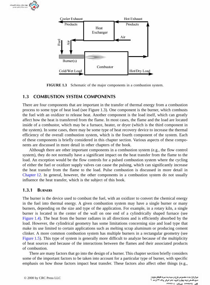
There are four components that are important in the transfer of thermal energy from a combustion process to some type of heat load (see Figure 1.3). One component is the burner, which combusts the fuel with an oxidizer to release heat. Another component is the load itself, which can greatly affect how the heat is transferred from the flame. In most cases, the flame and the load are located inside of a combustor, which may be a furnace, heater, or dryer (which is the third component in the system). In some cases, there may be some type of heat recovery device to increase the thermal efficiency of the overall combustion system, which is the fourth component of the system. Each of these components is briefly considered in this chapter section. Various aspects of these compo-nents are discussed in more detail in other chapters of the book.
Although there are other important components in a combustion system (e.g., the flow control system), they do not normally have a significant impact on the heat transfer from the flame to the load. An exception would be the flow controls for a pulsed combustion system where the cycling of either the fuel or oxidizer supply valves can cause the pulsing, which can significantly increase the heat transfer from the flame to the load. Pulse combustion is discussed in more detail in Chapter 12. In general, however, the other components in a combustion system do not usually influence the heat transfer, which is the subject of this book.
1.3.1 BURNERS
The burner is the device used to combust the fuel, with an oxidizer to convert the chemical energy in the fuel into thermal energy. A given combustion system may have a single burner or many burners, depending on the size and type of the application. For example, in a rotary kiln, a single burner is located in the center of the wall on one end of a cylindrically shaped furnace (see Figure 1.4). The heat from the burner radiates in all directions and is efficiently absorbed by the load. However, the cylindrical geometry has some limitations concerning size and load type that make its use limited to certain applications such as melting scrap aluminum or producing cement clinker. A more common combustion system has multiple burners in a rectangular geometry (see Figure 1.5). This type of system is generally more difficult to analyze because of the multiplicity of heat sources and because of the interactions between the flames and their associated products of combustion.
There are many factors that go into the design of a burner. This chapter section briefly considers some of the important factors to be taken into account for a particular type of burner, with specific emphasis on how those factors impact heat transfer. These factors also affect other things (e.g.,
FIGURE 1.3 Schematic of the major components in a combustion system.
© 2000 by CRC Press LLC

pollutant emissions), which will only briefly be discussed since they normally only influence the heat transfer characteristics for a given burner design under fairly limited and special conditions.
1.3.1.1 Competing Priorities
There have many changes in the traditional designs that have been used in burners, primarily because of the recent interest in reducing pollutant emissions. In the past, the burner designer was primarily concerned with efficiently combusting the fuel and transferring the energy to a heat load. New and increasingly more stringent environmental regulations have added the need to considerthe pollutant emissions produced by the burner. In many cases, reducing pollutant emissions and
FIGURE 1.4 Single burner in a rotary kiln.
FIGURE 1.5 Multiple burners in a side-fired regenerative glass furnace.
© 2000 by CRC Press LLC
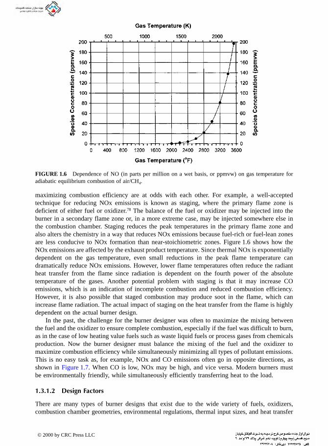
maximizing combustion efficiency are at odds with each other. For example, a well-accepted technique for reducing NOx emissions is known as staging, where the primary flame zone is deficient of either fuel or oxidizer.78 The balance of the fuel or oxidizer may be injected into the burner in a secondary flame zone or, in a more extreme case, may be injected somewhere else in the combustion chamber. Staging reduces the peak temperatures in the primary flame zone and also alters the chemistry in a way that reduces NOx emissions because fuel-rich or fuel-lean zones are less conducive to NOx formation than near-stoichiometric zones. Figure 1.6 shows how the NOx emissions are affected by the exhaust product temperature. Since thermal NOx is exponentially dependent on the gas temperature, even small reductions in the peak flame temperature can dramatically reduce NOx emissions. However, lower flame temperatures often reduce the radiant heat transfer from the flame since radiation is dependent on the fourth power of the absolute temperature of the gases. Another potential problem with staging is that it may increase CO emissions, which is an indication of incomplete combustion and reduced combustion efficiency. However, it is also possible that staged combustion may produce soot in the flame, which can increase flame radiation. The actual impact of staging on the heat transfer from the flame is highly dependent on the actual burner design.
In the past, the challenge for the burner designer was often to maximize the mixing between the fuel and the oxidizer to ensure complete combustion, especially if the fuel was difficult to burn, as in the case of low heating value fuels such as waste liquid fuels or process gases from chemicals production. Now the burner designer must balance the mixing of the fuel and the oxidizer to maximize combustion efficiency while simultaneously minimizing all types of pollutant emissions. This is no easy task as, for example, NOx and CO emissions often go in opposite directions, as shown in Figure 1.7. When CO is low, NOx may be high, and vice versa. Modern burners must be environmentally friendly, while simultaneously efficiently transferring heat to the load.
1.3.1.2 Design Factors
There are many types of burner designs that exist due to the wide variety of fuels, oxidizers, combustion chamber geometries, environmental regulations, thermal input sizes, and heat transfer
FIGURE 1.6 Dependence of NO (in parts per million on a wet basis, or ppmvw) on gas temperature for adiabatic equilibrium combustion of air/CH4.
© 2000 by CRC Press LLC

requirements, which includes things like flame temperature, flame momentum, and heat distribution. Some of these design factors are briefly considered here.
1.3.1.2.1 FuelDepending on many factors, certain types of fuels are preferred for certain geographic locations due to cost and availability considerations. Gaseous fuels — particularly natural gas — are com-monly used in most industrial heating applications in the U.S. In Europe, natural gas is also commonly used, along with light fuel oil. In Asia and South America, heavy fuel oils are generally preferred although the use of gaseous fuels is on the rise. Fuels also vary depending on the application. For example, in incineration processes, waste fuels are commonly used either by themselves or with other fuels like natural gas. In the petrochemical industry, fuel gases often consist of a blend of several fuels, including gases like hydrogen, methane, propane, butane, and propylene.
Fuel choice has an important influence on the heat transfer from a flame. In general, solid fuels like coal and liquid fuels like oil produce very luminous flames that contain soot particles that radiate like blackbodies to the heat load. Gaseous fuels like natural gas often produce nonluminous flames because they burn so cleanly and completely, without producing soot particles. A fuel like hydrogen is completely nonluminous, as there is no carbon available to produce soot. In cases where highly radiant flames are required, a luminous flame is preferred. In cases where convection heat transfer is preferred, a nonluminous flame may be preferred in order to minimize the possibility of contaminating the heat load with soot particles from a luminous flame. Where natural gas is the preferred fuel and highly radiant flames are desired, new technologies are being developed to produce more luminous flames. These include things like pyrolyzing the fuel in a partial oxidation process,79 using a plasma to produce soot in the fuel,80 and generally controlling the mixing of the fuel and oxidizer to produce fuel-rich flame zones that generate soot particles.81 Therefore, the fuel itself has a significant impact on the heat transfer mechanisms between the flame and the load. In most cases, the fuel choice is dictated by the customer as part of the specifications for the system and is not chosen by the burner designer. The designer must make the best of whatever fuel has been selected. In most cases, the burner design is optimized based on the choice for the fuel.
FIGURE 1.7 Dependence of NO and CO on equivalence ratio for adiabatic equilibrium air/CH4 flames.
© 2000 by CRC Press LLC

In some cases, the burner may have more than one type of fuel. An example is shown in Figure 1.8.82 Dual-fuel burners are typically designed to operate on either gaseous or liquid fuels. These burners are used where the customer may need to switch between a gaseous fuel like natural gas and a liquid fuel like oil, usually for economic reasons. These burners normally operate on one fuel or the other, and occasionally on both fuels. Another application where multiple fuels may be used is in waste incineration. One method of disposing of waste liquids contaminated with hydro-carbons is to combust them by direct injection through a burner. The waste liquids are fed through the burner, which is powered by a traditional fuel such as natural gas or oil. The waste liquids often have very low heating values and are difficult to combust without auxiliary fuel. This further complicates the burner design where the waste liquid must be vaporized and combusted concurrently with the normal fuel used in the burner.
1.3.1.2.2 OxidizerThe predominant oxidizer used in most industrial heating processes is atmospheric air. This can present challenges in some applications where highly accurate control is required due to the daily variations in the barometric pressure and humidity of ambient air. The combustion air is sometimes preheated and sometimes blended with some of the products of combustion, which is usually referred to as flue gas recirculation (FlGR). In certain cases, preheated air is used to increase the overall thermal efficiency of a process. FlGR is often used to both increase thermal efficiency and
FIGURE 1.8 Typical combination oil and gas burner. (Courtesy of American Petroleum Institute, Washing-ton, D.C.82 With permission.)
© 2000 by CRC Press LLC

reduce NOx emissions. The thermal efficiency is increased by capturing some of the energy in the exhaust gases that are used to preheat the incoming combustion oxidizer. NOx emissions can also
be reduced because the peak flame temperatures are reduced, which can reduce the NOx emissions, which are highly temperature dependent. There are also many high-temperature combustion pro-cesses that use an oxidizer containing a higher proportion of oxygen than the 21% (by volume) found in normal atmospheric air. This is referred to as oxygen-enhanced combustion (OEC) and has many benefits, which include increased productivity and thermal efficiency while reducing the exhaust gas volume and pollutant emissions.83 A simplified global chemical reaction for the stoichiometric combustion of methane with air is given as follows:
CH4 + 2O2 + 7.52N2 → CO2 + 2H2O + 7.52N2 + Trace species (1.1)
This compares to the same reaction where the oxidizer is pure O2 instead of air:
CH4 + 2O2 → CO2 + 2H2O + Trace species (1.2)
The volume of exhaust gases is significantly reduced by the elimination of N2. In general, a stoichiometric oxygen-enhanced methane combustion process can be represented by:
CH4 + 2O2 + xN2 →CO2 + 2H2O + xN2 + Trace species (1.3)
where 0 ð x ð 7.52, depending on the oxidizer. The N2 contained in air acts as a ballast that may inhibit the combustion process and have negative consequences. The benefits of using oxygen-enhanced combustion must be weighed against the added cost of the oxidizer, which in the case of air is essentially free except for the minor cost of the air-handling equipment and power for the blower. The use of a higher purity oxidizer has many consequences with regard to heat transfer from the flame, which are considered elsewhere in this book. Oxygen-enhanced combustion is considered in more detail in Chapter 12.
1.3.1.2.3 Gas recirculationA common technique used in combustion systems is to design the burner to induce furnace gases to be drawn into the burner to dilute the flame, usually referred to as furnace gas recirculation (FuGR). Although the furnace gases are hot, they are still much cooler than the flame itself. This dilution may accomplish several purposes. One is to minimize NOx emissions by reducing the peak temperatures in the flame, as in FlGR. However, furnace gas recirculation may be preferred to FlGR because no external high-temperature ductwork or fans are needed to bring the product gases into the flame zone. Another reason to use furnace gas recirculation may be to increase the convective heating from the flame because of the added gas volume and momentum. An example of flue gas recirculation into the burner is shown in Figure 1.9.84
1.3.1.3 General Burner Types
There are numerous ways to classify burners. Some of the common ones are discussed in this chapter section, with a brief consideration as to how the heat transfer is impacted.
1.3.1.3.1 Mixing typeA common method for classifying burners is according to how the fuel and the oxidizer are mixed. In premixed burners, shown in a cartoon in Figure 1.10 and schematically in Figure 1.11, the fuel and the oxidizer are completely mixed before combustion begins. Porous radiant burners are usually of the premixed type (see Chapter 8). Premixed burners often produce shorter and more intense flames, as compared to diffusion flames. This can produce high-temperature regions in the flame,
© 2000 by CRC Press LLC

leading to nonuniform heating of the load and higher NOx emissions. However, in flame impinge-ment heating, premixed burners are useful because the higher temperatures and shorter flames can enhance the heating rates (see Chapter 7).
In diffusion-mixed burners, shown schematically in Figure 1.12, the fuel and the oxidizer are separated and unmixed prior to combustion, which begins where the oxidizer/fuel mixture is within the flammability range. Oxygen/fuel burners (see Chapter 12) are usually diffusion burners, prima-rily for safety reasons, to prevent flashback and explosion in a potentially dangerous system. Diffusion gas burners are sometimes referred to as “raw gas” burners as the fuel gas exits the burner essentially intact with no air mixed with it. Diffusion burners typically have longer flames than premixed burners, do not have as high temperature a hotspot, and usually have a more uniform temperature and heat flux distribution.
It is also possible to have partially premixed burners, as shown schematically in Figures 1.11 and 1.13, where a portion of the fuel is mixed with the oxidizer. This is often done for stability and safety reasons where the partial premixing helps anchor the flame, but not fully premixing lessens the chance for flashback. This type of burner often has a flame length and temperature and heat flux distribution that is between the fully premixed and diffusion flames.
Another burner classification based on mixing is known as staging: staged air and staged fuel. A staged-air burner is shown in a cartoon in Figure 1.14 and schematically in Figure 1.15. A staged-fuel burner is shown in a cartoon in Figure 1.16 and schematically in Figure 1.17. Secondary and sometimes tertiary injectors in the burner are used to inject a portion of the fuel and/or the oxidizer into the flame, downstream of the root of the flame. Staging is often done to reduce NOx emissions and produce longer flames. These longer flames typically have a lower peak flame temperature and more uniform heat flux distribution than nonstaged flames.
1.3.1.3.2 Oxidizer typeBurners and flames are often classified according to the type of oxidizer used. The majority of industrial burners use air for combustion. In many of the higher temperature heating and melting
FIGURE 1.9 Schematic of flue gas recirculation.
FIGURE 1.10 Premix burner.
© 2000 by CRC Press LLC

FIGURE 1.11 Typical partially premixed gas burner. (Courtesy of American Petroleum Institute, Washing-ton, D.C.82 With permission.)
FIGURE 1.12 Diffusion burner.
FIGURE 1.13 Partially premixed burner.
© 2000 by CRC Press LLC

applications, such as glass production, the oxidizer is pure oxygen. In other applications, the oxidizer is a combination of air and oxygen, often referred to as oxygen-enriched air combustion. The latter two types of oxidizers are discussed in more detail in Chapter 12.
Another way to classify the oxidizer is by its temperature. It is common in many industrial applications to recover heat from the exhaust gases by preheating the incoming combustion air — either with a recuperator or a regenerator (discussed below). Such a burner is often referred to as a preheated air burner.
1.3.1.3.3 Draft typeMost industrial burners are known as forced-draft burners. This means that the oxidizer is supplied to the burner under pressure. For example, in a forced-draft air burner, the air used for combustion is supplied to the burner by a blower. In natural-draft burners, the air used for combustion is induced into the burner by the negative draft produced in the combustor. A schematic is shown in Figure 1.18 and an example is shown in Figure 1.19. In this type of burner, the pressure drop and combustor stack height are critical in producing enough suction to induce enough combustion air into the burners. This type of burner is commonly used in the chemical and petrochemical industries in
FIGURE 1.14 Staged-air burner.
FIGURE 1.15 Typical staged-air combination oil and gas burner. (Courtesy of John Zink Co. LLC, Tulsa, OK. With permission.)
FIGURE 1.16 Staged-fuel burner.
© 2000 by CRC Press LLC
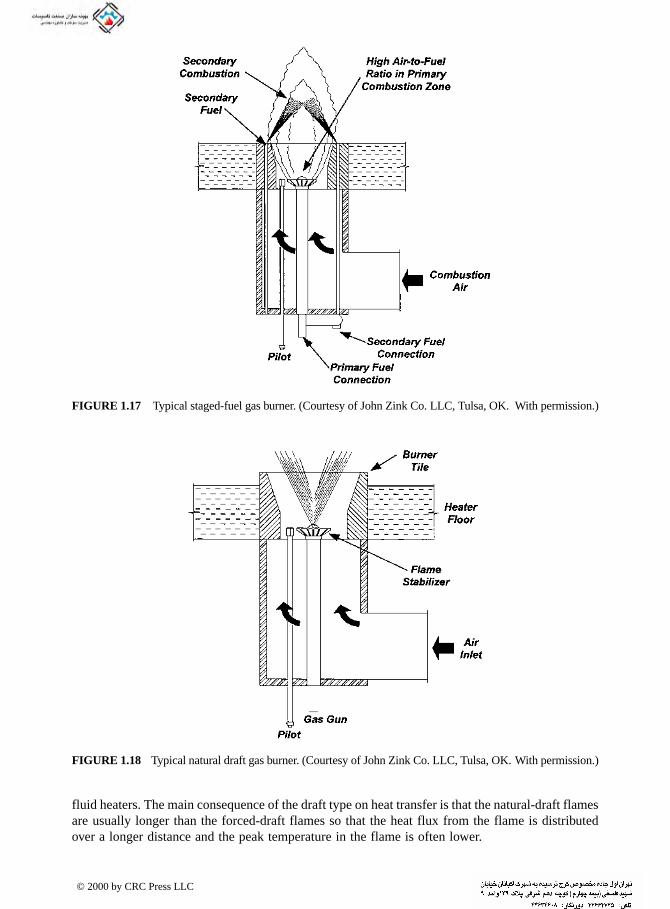
fluid heaters. The main consequence of the draft type on heat transfer is that the natural-draft flames are usually longer than the forced-draft flames so that the heat flux from the flame is distributed over a longer distance and the peak temperature in the flame is often lower.
FIGURE 1.17 Typical staged-fuel gas burner. (Courtesy of John Zink Co. LLC, Tulsa, OK. With permission.)
FIGURE 1.18 Typical natural draft gas burner. (Courtesy of John Zink Co. LLC, Tulsa, OK. With permission.)
© 2000 by CRC Press LLC

1.3.1.3.4 Heating typeBurners are often classified as to whether they are direct or indirect heating. In direct heating, there is no intermediate heat exchange surface between the flame and the load. In indirect heating, such as radiant tube burners (see Chapter 8), there is an intermediate surface between the flame and the load. This is usually done because the combustion products cannot come in contact with the load because of possible contamination.
1.3.2 COMBUSTORS
This chapter section briefly introduces the combustors that are commonly used in industrial heating and melting applications. These combustors are discussed in more detail in Chapters 9, 10, and 11.
1.3.2.1 Design Considerations
There are many important factors that must be considered when designing a combustor. This chapter section only briefly considers a few of those factors and how they may influence the heat transfer in the system.
1.3.2.1.1 Load handlingA primary consideration for any combustor is the type of material that will be processed. The various types of loads are considered later in this chapter and also in more detail in Chapter 4. One obvious factor of importance in handling the load and transporting it through the combustor is its physical state — whether it is a solid, liquid, or gas. Another factor is the transport properties of the load. For example, the solid might be granular or it might be in the form of a sheet (web). Related to this is how the solid will be fed into the combustor. A granular solid could be fed
FIGURE 1.19 Natural draft burner. (Courtesy of John Zink Co. LLC, Tulsa, OK. With permission.)
© 2000 by CRC Press LLC

continuously into a combustor with a screw conveyor or it could be fed in with discrete charges from a front-end loader. The shape of the furnace will vary according to how the material will be
transported through it. For example, limestone is fed continuously into a rotating and slightly downward-inclined cylinder.
1.3.2.1.2 TemperatureIn this book, industrial heating applications have been divided into two categories: higher and lower temperatures. The division between the two is somewhat arbitrary but mainly concerns the different types of applications used in each. For example, most of the metal- and glass-melting applications fall into the higher temperature categories, as the furnace temperatures are often well over 2000°F (1400K). They use technologies like air preheating and oxygen enrichment (see Chapter 12) to achieve those higher temperatures. Lower temperature applications include dryers, process heaters, and heat treating and are typically below about 2000°F (1400K). Although many of these processes may use air preheating, it is primarily to improve the thermal efficiency and not to get higher flame temperatures. Those processes rarely use oxygen enrichment, which usually only works econom-ically for higher temperature processes. Obviously, the combustors are designed differently for higher and lower temperature processes. The heat transfer mechanisms are often different as well. In higher temperature processes, the primary mode is often radiation, while in lower temperature applications, convection often plays a significant role.
1.3.2.1.3 Heat recoveryWhen heat recovery is used in an industrial combustion process, it is an integral part of the system. The two most popular methods are regenerative and recuperative, which are discussed briefly below and also in Chapter 8. The heat recovery system is important in the design of the combustor as it determines the thermal efficiency of the process and the flame temperatures in the system. It also influences the heat transfer modes as it may increase both the radiation and convection because of higher flame temperatures. Another type of heat recovery used in some processes is furnace or flue gas recirculation, where the exhaust products are recirculated back through the flame. This also influences the heat transfer and furnace design as it can moderate the flame temperature but increase the volume flow of gases through the combustion chamber.
1.3.2.2 General Classifications
There are several ways that a combustor can be classified; these are briefly discussed in this chapter section. Each type has an impact on the heat transfer mechanisms in the furnace.
1.3.2.2.1 Load processing methodFurnaces are often classified as to whether they are batch or continuous. In a batch furnace, the load is charged into the furnace at discrete intervals where it is heated. There may be multiple load charges, depending on the application. Normally, the firing rate of the burners is reduced or turned off during the charging cycle. On some furnaces, a door may also need to be opened during charging. These significantly impact the heat transfer in the system as the heat losses during the charge cycle are very large. The radiation losses through open doors are high and the reduced firing rate may not be enough to maintain the furnace temperature. In some cases, the temperature on the inside of the refractory wall, closest to the load, may actually be lower than the temperature of the refractory at some distance from the inside, due to the heat losses during charging. The heating process and heat transfer are dynamic and constantly changing as a result of the cyclical nature of the load charging. This makes analysis of these systems more complicated because of the need to include time in the computations.
In a continuous furnace, the load is constantly fed into and out of the combustor. The feed rate may change, sometimes due to conditions upstream or downstream of the combustor or due to the production needs of the plant, but the process is nearly steady state. This makes continuous processes
© 2000 by CRC Press LLC

simpler to analyze as there is no need to include time in the computations. It is often easier to make meaningful measurements in continuous processes due to their steady-state nature.
There are some furnaces that are semicontinuous, where the load may be charged in a nearly
continuous fashion, but the finished product may be removed from the furnace at discrete intervals. An example is an aluminum reverberatory furnace that is charged using an automatic side-well feed mechanism (see Chapter 11). In that process, shredded scrap is continuously added to a circulating bath of molten aluminum. When the correct alloy composition has been reached and the furnace has a full load, some or all of that load is then tapped out of the furnace. The effect on heat transfer is somewhere between that for batch and continuous furnaces.
1.3.2.2.2 Heating typeAs described above for burners, combustors are often classified as indirect or direct heating. In indirect heating, there is some type of intermediate heat transfer medium between the flames and the load that keeps the combustion products separate from the load. One example is a muffle furnace where there is a high-temperature ceramic muffle between the flames and the load. The flames transfer their heat to the muffle, which then radiates to the load which is usually some type of metal. The limitation of indirect heating processes is the temperature limit of the intermediate material. Although ceramic materials have fairly high temperature limits, other issues such as structural integrity over long distance spans and thermal cycling can still reduce the recommended operating temperatures. Another example of indirect heating is in process heaters where fluids are transported through metal tubes that are heated by flames. Indirect heating processes often have fairly uniform heat flux distributions because the heat exchange medium tends to homogenize the energy distribution from the flames to the load. The heat transfer from the heat exchange surface to the load is often fairly simple and straightforward to compute because of the absence of chemical reactions in-between. However, the heat transfer from the flames to the heat exchange surface and the subsequent thermal conduction through that surface are as complicated as if the flame was radiating directly to the load.
As a result of the temperature limits of the heat exchange materials, most higher temperature processes are of the direct heating type where the flames can directly radiate heat to the load.
1.3.2.2.3 GeometryAnother common way of classifying combustors is according to their geometry, which includes their shape and orientation. The two most common shapes are rectangular and cylindrical. The two most common orientations are horizontal and vertical, although inclined furnaces are commonly used in certain applications (e.g., rotary cement furnaces). An example of using the shape and orientation of the furnace as a means of classification would be a vertical cylindrical heater (sometimes referred to as a VC) used to heat fluids in the petrochemical industry. Both the furnace shape and orientation have important effects on the heat transfer in the system. They also determine the type of analysis that will be used. For example, in a VC heater, it is often possible to model only a slice of the heater due to its angular symmetry, in which case cylindrical coordinates would be used. On the other hand, it is usually not reasonable to model a horizontal rectangular furnace using cylindrical coordinates, especially if buoyancy effects are important.
Some furnaces are classified by what they look like. One example is a shaft furnace used to make iron. The raw materials are loaded into the top of a tall, thin, vertically oriented cylinder. Hot combustion gases generated at the bottom through the combustion of coke flow up through the raw materials which get heated. The melted final product is tapped out of the bottom. The furnace looks and acts almost like a shaft because of the way the raw materials are fed in through the top and exit at the bottom. A transfer chamber used to move molten metal around in a steel mill is often referred to as a ladle because of its function and appearance. These ladles are preheated using burners before the molten metal is poured into them to prevent the refractory-lined vessels from thermally shocking.
© 2000 by CRC Press LLC

Another aspect of the geometry that is important in some applications is whether the furnace is moving or not. For example, in a rotary furnace for melting scrap aluminum, the furnace rotates
to enhance mixing and heat transfer distribution. This again affects the type of analysis that would be appropriate for that system and can add some complexity to the computations.
The burner orientation with respect to the combustor is also sometimes used to classify the combustor. For example, a wall-fired furnace has burners located in and firing along the wall.
1.3.2.2.4 Heat recuperationIn many heat processing systems, energy recuperation is an integral part of the combustion system. Often, the heat recuperation equipment is a separate component of the system and not part of the burners themselves. Depending on the method used to recover the energy, the combustors are commonly referred to as either recuperative or regenerative (see discussion below). The heat transfer in these systems is a function of the energy recovery system. For example, the higher the combustion air preheat temperature, the hotter the flame and the more radiant heat that can be produced by that flame. The convective heat transfer may also be increased due to the higher gas temperature and also due to the higher thermal expansion of the gases which increases the average gas velocity through the combustor.
1.3.3 HEAT LOAD
This chapter section is a brief introduction to some of the important issues concerning the heat load in a furnace or combustor. A more detailed treatment is given in Chapter 4.
1.3.3.1 Process Tubes
In petrochemical production processes, process heaters are used to heat petroleum products to operating temperatures. The fluids are transported through the process heaters in process tubes. These heaters often have a radiant section and a convection section. In the radiant section, radiation from burners heats the process tubes. In the convection section, the combustion products heat the tubes by flowing over the tubes. The design of the radiant section is especially important because flame impingement on the tubes can cause premature failure of the tubes or cause the hydrocarbon fluids to coke inside the tubes, which reduces the heat transfer to the fluids.
1.3.3.2 Moving Substrate
In some applications, heaters and burners are used to heat or dry moving substrates or webs. An example is shown in Figure 1.20. One common application is the use of gas-fired infrared (IR) burners to remove moisture from paper during the forming process.85 These paper webs can travel at speeds over 300 m/s (1000 ft/s) and are normally dried by traveling over and contacting steam-heated cylinders. IR heaters are often used to selectively dry certain portions of the web that may be wetter than others. For example, if the target moisture content for the paper is 5%, then the entire width of the paper must have no more than 5% moisture. Streaks of higher moisture areas
FIGURE 1.20 Gas-fired infrared burners heating a moving substrate.
© 2000 by CRC Press LLC

often occur in sections along the width of the paper. Without selectively drying those areas, those streaks would be dried to the target moisture level, which means that the rest of the sheet would
be dried to even lower moisture levels. This creates at least two important problems. The first is lost revenue because paper is usually sold on a weight basis; any water unnecessarily removed from the paper decreases its weight and therefore results in lost income. Another problem is a reduction in the quality of the paper. If areas of the paper are too dry, they do not handle as well in devices like copiers and printers and are not nearly as desirable as paper of uniform moisture content. Therefore, selective drying of the paper only removes the minimum amount of water from the substrate. The challenge of this application is to measure the moisture content profile across the width of a sheet that may be several meters wide and moving at hundreds of meters per second. That information must then be fed to the control system for the IR heaters, which then must be able to react almost instantaneously. This is possible today because of advances in measurement and controls systems.
Another example of a moving substrate application is using IR burners to remove water during the production of fabrics in textile manufacturing.86 Moving substrates present unique challenges for burners. Often, the material being heated can easily be set on fire if there is a line stoppage and the burner is not turned off quickly enough. This means that the burner control system must be interlocked with the web-handling equipment so that the burners can be turned off immediately in the event of a line stoppage. If the burners have substantial thermal mass, then the burners may need to be retracted away from the substrate during a stoppage, or heat shields may need to be inserted between the burners and the substrate to prevent overheating.
Convection dryers are also used to heat and dry substrates. Typically, high-velocity heated air is blown at the substrate from both sides so that the substrate is elevated between the nozzles. In many cases, the heated air is used for both heat and mass transfer, to volatilize any liquids on or in the substrate such as water, and then carry the vapor away from the substrate.
An important aspect of heating webs is how the energy is transferred into the material. For example, dry paper is known to be a good insulator. When steam cylinders are used to heat and dry paper, they become less and less effective as the paper becomes drier because the heat from the cylinder cannot conduct through the paper as well as when it is moist since the thermal conductivity of the paper increases with moisture content. IR burners are effective for drying paper because the radiant energy transfers into the paper and is absorbed by the water. The radiant penetration into the paper actually increases as the paper becomes drier, unlike with steam cylinders which become less effective.
1.3.3.3 Opaque Materials
This type of load encompasses a wide range of materials, including granular solids like limestone and liquids like molten metal. For this type of load, the heat transfers to the surface of the load and must conduct down into the material. This process can be enhanced by proper mixing of the materials so that new material is constantly exposed to the surface, as in rotary kilns or in aluminum rever-beratory furnaces which have molten metal pumps to continuously recirculate the metal through the heating zone. The potential problems with this method include overheating the surface materials or having lower thermal efficiencies by limiting the heat transfer to the surface to prevent overheating.
1.3.3.4 Transparent Materials
The primary example of this type of load is glass, which has selective radiant transmission properties. In glass-melting processes (see Chapter 11), the primary mode of heat transfer is by radiation. As shown in Chapter 3, flames have specific types of radiant outputs that vary as a function of wavelength. If the flame is nonluminous, the flame usually has higher radiant outputs in the preferred wavelengths for water and carbon dioxide bands. If the flame is luminous, it has
© 2000 by CRC Press LLC

a broader, more graybody-type spectral radiant profile. Chapter 4 shows that luminous flames are preferred in melting glass because of the selective transmission properties of molten glass. This
allows a significant portion of the radiation received at the surface of the glass to penetrate into the glass, which enhances heat transfer rates and reduces the chances of overheating the surface, which would reduce product quality.
1.3.4 HEAT RECOVERY DEVICES
Heat recovery devices are often used to improve the efficiency of combustion systems. Some of these devices are incorporated into the burners, but more commonly they are another component in the combustion system, separate from the burners. These heat recovery devices incorporate some type of heat exchanger, depending on the application. The two most common types have been recuperators and regenerators, which are briefly discussed next. A fuller treatment of this topic is contained in Chapter 9. Reed (1987) predicts an increasing importance for heat recovery devices in industrial combustion systems for increasing heat transfer and thermal efficiencies.87
1.3.4.1 Recuperators
A recuperator is a low- to medium-temperature (up to about 1300°F, or 700°C), continuous heat exchanger that uses the sensible energy from hot combustion products to preheat the incoming combustion air. These heat exchangers are commonly counterflow, where the highest temperatures for both the combustion products and the combustion air are at one end of the exchanger with the coldest temperatures at the other end. Lower temperature recuperators are normally made of metal, while higher temperature recuperators may be made of ceramics. Recuperators are typically used in lower temperature applications because of the limitations of the metals used to construct these heat exchangers. These are discussed in more detail in section 9.3.1.
1.3.4.2 Regenerators
A regenerator is a higher temperature, transient heat exchanger used to improve the energy efficiency of high-temperature heating and melting processes, particularly in the high-temperature processing industries like glass production. In a regenerator, energy from the hot combustion products is temporarily stored in a unit constructed of firebricks. This energy is then used to heat the incoming combustion air during a given part of the firing cycle up to temperatures in excess of 2000°F (1000°C).
Regenerators are normally operated in pairs. During one part of the cycle, the hot combustion gases are flowing through one of the regenerators and heating up the refractory bricks, while the combustion air is flowing through and cooling down the refractory bricks in the second regenerator. Both the exhaust gases and the combustion air directly contact the bricks in the regenerators, although not both at the same time since each is in a different regenerator at any given time. After a sufficient amount of time (usually from 5 to 30 min), the cycle is reversed so that the cooler bricks in the second regenerator are then reheated while the hotter bricks in the first regenerator exchange their heat with the incoming combustion air. A reversing valve is used to change the flow from one gas to another in each regenerator. These are discussed further in section 9.3.2.
Davies (1986) noted that some of the following questions should be considered concerning regenerative burners:88
• What will the fuel savings be (compared to no heat recuperation)?• What is the maximum allowable flue gas temperature?• How big is the heat exchanger?• What is the air pressure drop through the exchanger?
© 2000 by CRC Press LLC

• How long will the exchanger run without plugging?• Is the flue gas path through the furnace altered?
REFERENCES
1. G.F. Hewitt, G.L. Shires, and T.R. Bott, Process Heat Transfer, CRC Press, Boca Raton, FL, 1994.2. U.S. Department of Energy, Energy Information Administration, Annual Energy Outlook 1999, Report
DOE/EIA-0383(99) Washington, D.C.3. R.J. Reid, What You Should Know About Combustion, Glass Industry, 70(7), 24-35, 1989.4. D.F. Knowles, Combustion system requirements for advanced gas-fired processes, in Industrial Com-
bustion Technologies, M.A. Lukasiewicz, Ed., American Society of Metals, Warren, PA, 1986, 323-325.
5. J.H. Pohl, W.S. Lanier, J. Keller, J. Patton, and R. Jain, Technologies to increase the efficient use of energy in the process industries, in Industrial Combustion Technologies, M.A. Lukasiewicz, Ed., American Society of Metals, Warren, PA, 1986, 313-321.
6. J.D. Wilde, Combustion problems in the steel industry, in Industrial Combustion Technologies, M.A. Lukasiewicz, Ed., American Society of Metals, Warren, PA, 1986, 13-22.
7. R.A. Drake, Combustion progress, problems, needs in the glass industry, in Industrial Combustion Technologies, M.A. Lukasiewicz, Ed., American Society of Metals, Warren, PA, 1986, 23-25.
8. A. Gupta and D.G. Lilley, An overview of research needs in practical combustion systems, in Heat Transfer in Furnaces, C. Presser and D.G. Lilley, Eds., New York, ASME HTD-Vol. 74, 1-10, 1987.
9. A.S. Chace, H.R. Hazard, A. Levy, A.C. Thekdi, and E.W. Ungar, Combustion Research Opportunities for Industrial Applications, U.S. Department of Energy Report DOE/ID-10204-2, 1989.
10. R. Viskanta, Enhancement of heat transfer in industrial combustion systems: problems and future challenges, in Thermal Engineering 1991, Proceedings of the ASME/JSME Joint Conference, J.R. Lloyd and Y. Kurosaki, Eds., ASME, 5, 161-173, 1991.
11. J.G. Keller, N.R. Soelberg, and G.F. Kessinger, Industry-Identified Combustion Research Needs, Idaho National Engineering Lab report INEL-95/0578, Idaho Falls, ID, 1995.
12. H.S. Kurek, M. Khinkis, W. Kunc, A. Touzet, A. de La Faire, T. Landais, A. Yerinov, and O. Semernin, Flat radiant panels for improving temperature uniformity and product quality in indirect-fired furnaces, Proc. of 1998 International Gas Research Conf., Vol. V: Industrial Utilization, D.A. Dolenc, Ed., Gas Research Institute, Chicago, 1998, 15-23.
13. U.S. Department of Energy, Industrial Combustion Technology Roadmap, Washington, D.C., April 1999.
14. B. Gebhart, Heat Transfer, 2nd edition, McGraw-Hill, New York, 1971.15. F. Kreith and M.S. Bohn, Principles of Heat Transfer, Harper & Row, New York, 1986.16. J.P. Holman, Heat Transfer, 7th edition, McGraw-Hill, New York, 1990.17. A. Bejan, Heat Transfer, Wiley, New York, 1993.18. F.P. Incropera and D.P. Dewitt, Introduction to Heat Transfer, 3rd edition, Wiley, New York, 1996.19. A.F. Mills, Heat Transfer, 2nd edition, Prentice-Hall, Englewood Cliffs, NJ, 1998.
19a. W.S. Janna, Engineering Heat Transfer, 2nd edition, CRC Press, Boca Raton, FL, 2000.20. H.C. Hottel and A.F. Sarofim, Radiative Transfer, McGraw-Hill, New York, 1967.21. T.J. Love, Radiative Heat Transfer, Merrill Publishing, Columbus, OH, 1968.22. M. Özisik, Radiative Transfer and Interactions with Conduction and Convection, Wiley, New York, 1973.23. W.A. Gray and R. Müller, Engineering Calculations in Radiative Heat Transfer, Pergamon, Oxford,
U.K., 1974.24. E.M. Sparrow and R.D. Cess, Radiation Heat Transfer, augmented edition, Hemisphere, Washington,
D.C., 1978.25. J.B. Dwyer, Furnace calculations, in Process Heat Transfer, D.Q. Kern, Ed., McGraw-Hill, New York,
1950.26. F.W. Hutchinson, Industrial Heat Transfer, Industrial Press, New York, 1952.27. S.T. Hsu, Engineering Heat Transfer, D. Van Nostrand Co., Princeton, NJ, 1963.28. J.R. Welty, Engineering Heat Transfer, Wiley, New York, 1974.29. B.V. Karlekar and R.M. Desmond, Engineering Heat Transfer, West Publ. Co., St. Paul, MN, 1977.
© 2000 by CRC Press LLC

30. V. Ganapathy, Applied Heat Transfer, PennWell Books, Tulsa, OK, 1982.31. A.G. Blokh, Heat Transfer in Steam Boiler Furnaces, Hemisphere, Washington, D.C., 1988.
32. W.M. Rohsenow, J.P., Hartnett, and E.N., Ganic, Handbook of Heat Transfer Applications, McGraw-
Hill Book Company, New York, 1985.33. N.P. Cheremisinoff, Ed., Handbook of Heat and Mass Transfer, 4 volumes, Gulf Pub. Co., Houston,
TX, 1986, Vol. 1: Heat Transfer Operations, Vol. 2: Mass Transfer and Reactor Design, Vol. 3: Catalysis, Kinetics, and Reactor Engineering, and Vol. 4: Advances in Reactor Design and Combustion Science.
34. F. Kreith, Ed., The CRC Handbook of Thermal Engineering, CRC Press, Boca Raton, FL, 2000.35. R.A. Strehlow, Fundamentals of Combustion, Inter. Textbook Co., Scranton, PA, 1968.36. F.A. Williams, Combustion Theory, Benjamin/Cummings Publishing, Menlo Park, CA, 1985.37. B. Lewis and G. von Elbe, Combustion, Flames and Explosions of Gases, 3rd edition, Academic
Press, New York, 1987.38. W. Bartok and A.F. Sarofim, Eds., Fossil Fuel Combustion, Wiley, New York, 1991.
38a. R.M. Fristrom, Flame Structure and Processes, Oxford University Press, New York, 1995.39. I. Glassman, Combustion, 3rd edition, Academic Press, New York, 1996.40. J.A. Barnard and J.N. Bradley, Flame and Combustion, 2nd edition, Chapman and Hall, London, 1985.41. S.R. Turns, An Introduction to Combustion, McGraw-Hill, New York, 1996.42. J. Griswold, Fuels, Combustion and Furnaces, McGraw-Hill, New York, 1946.43. A. Stambuleanu, Flame Combustion Processes in Industry, Abacus Press, Tunbridge Wells, U.K., 1976.44. E. Perthuis, La Combustion Industrielle, Éditions Technip, Paris, 1983.45. E.L. Keating, Applied Combustion, Marcel Dekker, New York, 1993.46. G. Borman and K. Ragland, Combustion Engineering, McGraw-Hill, New York, 1998.47. C.G. Segeler, Ed., Gas Engineers Handbook, Industrial Press, New York, 1965.48. R.D. Reed, Furnace Operations, 3rd edition, Gulf Publishing, Houston, 1976.49. R. Pritchard, J.J., Guy, and N.E., Connor, Handbook of Industrial Gas Utilization, Van Nostrand
Reinhold, New York, 1977.50. R.J. Reed, North American Combustion Handbook, Volume I, 3rd edition, North American Mfg. Co.,
Cleveland, OH, 1986.51. IHEA, Combustion Technology Manual, 5th edition, Industrial Heating Equipment Assoc., Arlington,
VA, 1994.52. W. Trinks and M.H., Mawhinney, Industrial Furnaces, Vol. I, 5th edition, John Wiley & Sons, New
York, 1961.53. A.E. Aldersley, Fuels, Combustion and Heat Transfer, Brick Development Association, London, 1964.54. W.A. Gray, J.K. Kilham, and R. Muller, Heat Transfer from Flames, Elek, London, 197655. E. E. Khalil, Modelling of Furnaces and Combustors, Abacus Press, Tunbridge Wells, Kent, 1982.56. J.M. Rhine, and R.J. Tucker, Modelling of Gas-Fired Furnaces and Boilers, McGraw-Hill, London, 1991.
56a. J.R. Cornforth, Ed., Combustion Engineering and Gas Utilisation, E&FN Spon, London, 1992.57. K.H. Khalil, F.M. El-Mahallawy, and E.E. Khalil, Eds., Flow, Mixing, and Heat Transfer in Furnaces,
Conference on Mechanical Power Engineering (1st: 1977, Cairo University), Pergamon Press, Oxford, U.K., 1978.
58. R. Lazzeretti and S.N.B. Murthy, Eds., Proceedings of the United States-Italy Joint Workshop on Heat Transfer and Combustion, U.S.A.-Italy Joint Workshop on Heat Transfer and Combustion (1982: Pisa, Italy), sponsored by the National Science Foundation and Consiglio nazionale della ricerche, s.n., 3 volumes, 1982.
59. C.K. Law, Ed., Heat transfer in fire and combustion systems, presented at the 23rd National Heat Transfer Conference, Denver, CO, August 4-7, 1985, sponsored by the K-11 Committee on Heat Transfer in Fire and Combustion Systems, the Heat Transfer Division, ASME, New York, HTD, Vol. 45, 1985.
60. C. Presser and D.G. Lilley, Eds., Heat transfer in furnaces, presented at the 24th National Heat Transfer Conference and Exhibition, Pittsburgh, PA, August 9-12, 1987, sponsored by the Heat Transfer Division, ASME, New York, HTD Vol. 74, 1987.
61. R.K. Shah, Ed., Heat transfer phenomena in radiation, combustion, and fires, presented at the 1989 National Heat Transfer Conference, Philadelphia, PA, August 6-9, 1989, sponsored by the Heat Transfer Division, ASME, New York, HTD Vol. 106, 1989.
© 2000 by CRC Press LLC

62. N. Ashgriz, Ed., Heat transfer in combustion systems, Proceedings of the Winter Annual Meeting of the American Society of Mechanical Engineers, San Francisco, CA, December 10-15, 1989, sponsored
by the Heat Transfer Division, ASME, New York, HTD Vol. 122, 1989.
63. B. Farouk, Ed., Heat transfer in combustion systems, presented at AIAA/ASME Thermophysics and Heat Transfer Conference, June 18-20, 1990, Seattle, WA, sponsored by the Heat Transfer Division, ASME, New York, HTD Vol. 142, 1990.
64. W.L. Grosshandler and H.G. Semerjian, Eds., Heat and mass transfer in fires and combustion systems, presented at the Winter Annual Meeting of the American Society of Mechanical Engineers, Dallas, TX, November 25-30, 1990, sponsored by the Heat Transfer Division, ASME, New York, HTD Vol. 148, 1990.
65. M.G. Carvalho, F. Lockwood, and J. Taine, Eds., Heat transfer in radiating and combusting systems, Proceedings of Eurotherm Seminar no. 17, 8-10 October 1990, Cascais, Portugal, Springer-Verlag, Berlin, 1991.
66. R.J. Santoro and J.D. Felske, Eds., Heat transfer in fire and combustion systems, 1991, presented at the 28th National Heat Transfer Conference, Minneapolis, MN, July 28-31, 1991, sponsored by the Heat Transfer Division, ASME, New York, HTD Vol. 166, 1991.
67. M.F. Modest, T.W. Simon, and M. Ali Ebadian, Eds., Experimental/numerical heat transfer in com-bustion and phase change, presented at the 28th National Heat Transfer Conference, Minneapolis, MN, July 28-31, 1991, sponsored by the Heat Transfer Division, ASME, New York, HTD, Vol. 170, 1991.
68. S.C. Yao and J.N. Chung, Eds., Heat and mass transfer in fires and combustion systems, presented at the Winter Annual Meeting of the American Society of Mechanical Engineers, Atlanta, GA, Decem-ber 1-6, 1991, sponsored by the Heat Transfer Division, ASME, New York, HTD Vol. 176, 1991.
69. A.M. Kanury and M.Q. Brewster, Eds., Heat transfer in fire and combustion systems, presented at the 28th National Heat Transfer Conference and Exhibition, San Diego, CA, August 9-12, 1992, sponsored by the Heat Transfer Division, ASME, New York, HTD Vol. 199, 1992.
70. P. Cho and J. Quintiere, Eds., Heat and mass transfer in fire and combustion systems, 1992: presented at the Winter Annual Meeting of the American Society of Mech. Engineers, Anaheim, CA, November 8-13, 1992, sponsored by the Heat Transfer Division, ASME, New York, HTD Vol. 223, 1992.
71. B. Farouk, M. P. Menguc, R. Viskanta, C. Presser, and S. Chellaiah Eds., Heat transfer in fire and combustion systems, presented at the 29th National Heat Transfer Conference, Atlanta, GA, August 8-11, 1993, sponsored by the Heat Transfer Division, ASME, New York, HTD Vol. 250, 1993.
72. W.W. Yuen, and K.S. Ball, Eds., Heat transfer in fire and combustion systems, presented at the 6th AIAA/ASME Thermophysics and Heat Transfer Conference, Colorado Springs, CO, June 20-23, 1994, sponsored by the Heat Transfer Division, ASME, New York, HTD Vol. 272, 1994.
73. R.B. Peterson, O.A. Ezekoye, and T. Simon, Combustion and fire research, Proceedings of the 1995 National Heat Transfer Conference, August 6-8 1995, Portland, OR, sponsored by the Heat Transfer Division, ASME, Vol. 2, 1995.
74. M.C. McQuay, K. Annamalai, W. Schreiber, D. Choudhury, E. Bigzadeh, and A. Runchal, Eds., Heat transfer in combustion systems, Proceedings of the 1996 31st National Heat Transfer Conference,Houston, TX, August 3-6 1996, sponsored by the Heat Transfer Division, ASME, New York, HTD Vol. 328, 1996.
75. K. Annamalai, S. Acharya, A.K. Gupta, R. Altenkirch, and C. Presser, Eds., Symposium on Fire and Combustion, Proc. of 32nd National Heat Transfer Conference, August 10-12, 1997, Baltimore, MD, sponsored by the Heat Transfer Division, ASME HTD-Vol. 352, New York, 1997.
76. R.A. Nelson, K.S. Ball, and Z.M. Zhang, Eds., Combustion and radiation heat transfer, Proceedings of the ASME Heat Transfer Division – 1998, Vol. 2, ASME HTD-Vol. 361-2, ASME, New York, 1998.
77. S.W. Churchill and N. Lior, Heat transfer in combustion chambers, Heat Transfer 1982, Vol. 1: Review and Keynote Papers, U. Grigull, E. Hahne, K. Stephan, and J. Straub, Eds., Hemisphere, Washington, D.C., 1982, 289-299.
78. J.L. Reese, G.L. Moilanen, R. Borkowicz, C. Baukal, D. Czerniak, and R. Batten, State-of-the-Art of NOx Emission Control Technology, ASME paper 94-JPGC-EC-15, Proceedings of Int. Joint Power Generation Conf., Phoenix, AZ, 3-5 October, 1994.
79. M.L. Joshi, M.E. Tester, G.C. Neff, and S.K. Panahi, Flame particle seeding with oxygen enrichment for NOx reduction and increased efficiency, Glass, 68(6), 212-213, 1990.
© 2000 by CRC Press LLC

80. R. Ruiz and J.C. Hilliard, Luminosity enhancement of natural gas flames, Proc. of 1989 International Gas Research Conf., T.L. Cramer, Ed., Govt. Institutes, Rockville, MD, 1990, 1345-1353.
81. A.G. Slavejkov, T.M. Gosling, and R.E. Knorr, Low-NOx Staged Combustion Device for Controlled
Radiative Heating in High Temperature Furnaces, U.S. patent 5,611,682, March 18, 1997.82. API Publication 535: Burner for Fired Heaters in General Refinery Services, 1st edition, American
Petroleum Institute, Washington, D.C., July 1995.83. C.E. Baukal, Ed., Oxygen-Enhanced Combustion, CRC Press, Boca Raton, FL, 1998.84. K.J. Fioravanti, L.S. Zelson, and C.E. Baukal, Flame Stabilized Oxy-Fuel Recirculating Burner, U.S.
Patent 4,954,076 issued 04 September 1990.85. S. Longacre, Using infrared to dry paper and its coatings, Process Heating, 4(2), 45-49, 1997.86. T.M. Smith and C.E. Baukal, Space-age refractory fibers improve gas-fired infrared generators for
heat processing textile webs, Journal of Coated Fabrics, 12(3), 160-173, 1983.87. R.J. Reed, Future consequences of compact, highly effective heat recovery devices, in Heat Transfer
in Furnaces, C. Presser and D.G. Lilley, Eds., ASME HTD, New York, 74, 23-28, 1987.88. T. Davies, Regenerative burners for radiant tubes — field test experience, in Industrial Combustion
Technologies, M.A. Lukasiewicz, Ed., American Society of Metals, Warren, PA, 1986, 65-70.
© 2000 by CRC Press LLC

Some Fundamentals
0-8493-7686-6/97/$0.00+$.50© 1997 by CRC Press LLC
2of Combustion
2.1 COMBUSTION CHEMISTRY
Combustion is usually considered to be the controlled release of heat and energy from the chemical reaction between a fuel and an oxidizer. This is in contrast to a fire or explosion which are usually uncontrolled and undesirable. Virtually all of the combustion in industrial processes uses a hydro-carbon fuel. A generalized combustion reaction for a typical hydrocarbon fuel can be written as follows:
fuel + oxidizer → CO2 + H2O + Other species (2.1)
The “other species” depends on what oxidizer is used and what is the ratio of the fuel to oxidizer. The most commonly used oxidizer is air, which consists of nearly 79% N2 by volume and is normally carried through in the combustion process. If the combustion is fuel rich, meaning there is not enough oxygen to fully combust the fuel, then there will be unburned hydrocarbons in the exhaust products and little if any excess O2. If the combustion is fuel lean, meaning there is more oxygen than required to fully combust the fuel, then there will be excess O2 in the exhaust products. The exhaust gas composition is very important in determining the heat transfer in the system. Unburned hydrocarbons in the exhaust indicate that the fuel was not fully combusted and therefore not all of the available heat was released. High excess O2 levels in the exhaust usually indicate that too much oxidizer was supplied. The excess oxidizer carries sensible energy out the exhaust, which again means that some of the available heat of the fuel was not fully utilized to heat the load. If the oxidizer is air, then a large proportion of the available energy in the fuel will normally be carried out the flue with the exhaust products. This is discussed in more detail in Chapter 12.
2.1.1 FUEL PROPERTIES
Table E.2 in Appendix E gives some of the properties for gaseous fuels commonly used in industrial combustion systems. As expected, the fuel has a significant influence on the heat transfer in a combustion system. One of the most important properties is the heating value of the fuel. This is used to determine how much fuel must be combusted to process the desired production rate of material that is being heated. The heating value is specified as either the higher heating value (HHV) or the lower heating value (LHV). The LHV excludes the heat of vaporization, which is the energy required to convert liquid water to steam. This means that the LHV assumes all of the products of combustion are gaseous, which is generally the case for nearly all industrial combustion applications. If the combustion products were to exit the process at a temperature low enough that all of the water is converted from a gas to a liquid, then the heat of condensation would be released into the process as an additional source of energy. The HHV of a fuel includes that energy.
The composition of the fuel is important in determining the composition of the products of combustion and the amount of oxidizer that will be needed to combust the fuel, both of which are discussed below. It is also important for determining the soot-producing tendency of the fuel which is discussed in Chapter 3. The density of the fuel is needed to determine flow rates through the fuel delivery system and the associated pipe sizes.
© 2000 by CRC Press LLC

2.1.2 OXIDIZER COMPOSITION
There are two common types of oxidizers used in industrial combustion processes. The majority
of those processes use air as the oxidizer. However, many of the higher temperature processes use an oxidizer containing a higher concentration of oxygen than found in air (approximately 21% by volume). This type of combustion is referred to as oxygen-enhanced combustion and is discussed further in Chapter 12.1 In many cases, the production rate in a heating process can be significantly increased with only relatively small amounts of oxygen enrichment. In most cases, air/fuel burners can successfully operate with an oxidizer containing up to about 30% O2 with little or no modifi-cations.2 At greater oxygen concentrations, the flame may become unstable or the flame temperature may become too high for a burner designed to operate under air/fuel conditions. In higher temper-ature applications where the benefits of higher purity oxygen justify the added costs, higher purity oxidizers may be used (>90% O2). The heating process is greatly intensified by the high purity oxygen. It has only been in the last decade that a significant number of combustion systems have been operated in the intermediate oxygen purities (30 – 90% O2), primarily for economic reasons as the cost of high-purity oxidizers is not justified. The oxidizer purity has a significant influence on the heat transfer in a combustion system, as will be shown throughout this book.
2.1.3 MIXTURE RATIO
An important consideration when studying a combustion system is the ratio of the fuel to the oxidizer. There are many ways that this can be specified. These are briefly considered here.
A global combustion reaction using CH4 as the fuel can be written as:
CH4 + (xO2 + yN2) → CO, CO2, H2, H2O, N2, NOx, O2, Trace species (2.2)
The stoichiometry of a reaction indicates the ratio of oxygen to fuel for a given system. One method of quantifying the stoichiometry is to only consider the O2 in the oxidizer, since the inerts in the oxidizer are not needed for the reaction:
(2.3)
If CH4 is again used as an example, a global simplified stoichiometric reaction with air can be written as:
CH4 + (2O2 + 7.52N2) → CO2 + 2H2O + 7.52N2 (2.4)
where air is represented as 2O2 + 7.52N2. In that case,
This method of specifying stoichiometry is more commonly used for combustion systems incor-porating oxygen enrichment. This is because the oxidizer composition can vary widely, but the amount of oxygen supplied to the combustion system is what is of importance.
The most common way of defining the stoichiometry or mixture ratio in industry in the U.S. is as follows:
(2.5)
S1 = Volume flow rate of O in the oxidizer
Volume flow rate of fuel2
S1
21
2= =
S2 = Volume flow rate of oxidizerVolume flow rate of fuel
© 2000 by CRC Press LLC

For the example reaction given in Equation 2.4, this stoichiometry would be calculated as follows:
The problem with the stoichiometry definition commonly used in industry (S2) is that the stoichi-ometry must be recalculated whenever the oxidizer composition changes and stoichiometric con-ditions change for each oxidizer composition. This is not a concern if air is always used as the oxidizer, which is the case for the vast majority of combustion processes. For example, consider the reaction of methane and pure oxygen:
CH4 + 2O2 → CO2 + 2H2O + 7.52N2 (2.6)
The two stoichiometric ratios would be calculated as follows:
For this limited case where the oxidizer is pure O2, S1 = S2; but in the example above using air as the oxidizer, S1 ¦ S2. For both cases, S1 is the same, while S2 is different. The benefit of using S1 is that the stoichiometry is independent of the oxidizer composition, so stoichiometric conditions are the same for any oxidizer composition. In Equation 2.1, S1 = x/1 = x. Theoretically, for the complete combustion of CH4 with no excess O2, S1 = 2.0, no matter how much N2 is in the oxidizer, while S2 varies depending on the actual N2 content in the oxidizer, although the same amount of O2 may be present. One can define the stoichiometric ratio for theoretically perfect combustion as S P
1 , which is equal to 2.0 for methane, no matter what the quantity of other gases besides O2 in the oxidizer. Then, the stoichiometric ratio for theoretical combustion for S2 would be S P
2 which, unlike S P1 , would
vary depending on the actual oxidizer composition.Actual flames generally require some excess O2 for complete combustion of the fuel. This is
due to incomplete mixing between the fuel and oxidant. For the fuel-rich combustion of CH4, S1 < 2.0. For the fuel-lean combustion of CH4, S1 > 2.0. These generalizations are not possible for S2
without specifying the oxidizer composition first.A common way of specifying the oxidizer composition is by calculating the O2 mole fraction
in the oxidizer, which can be defined as:
(2.7)
Using Equation 2.1, Ω = x/(x + y). If the oxidizer is air that contains approximately 21% O2 by volume, then Ω = 0.21. If the oxidizer is pure O2, then Ω = 1.0. The O2 enrichment level is sometimes used. This refers to the incremental O2 volume above that found in air. For example, if Ω = 0.35, then the O2 enrichment would be 14% (35% – 21% = 14%).
Another way of specifying the fuel mixture ratio is:
(2.8)
The way it is commonly specified in industry in Europe is as follows:
S2
2 7 521
9 52= + =..
S S1 2
21
221
2= = = =,
Ω = Volume flow rate of O in the oxidizer
Total volume flow rate of oxidizer2
λ1 = Actual volumetric ratio of oxygen:fuelStoichiometric volumetric ratio of oxygen:fuel
© 2000 by CRC Press LLC

(2.9)λ2 = Actual volumetric ratio of oxidant:fuel
Stoichiometric volumetric ratio of oxidant:fuel
or
(2.10)
Using this definition for the mixture ratio, λi < 1.0 for fuel-rich flames and λi > 1.0 for fuel-lean flames. Many industrial combustion processes run with approximately 3% more O2 than is theo-retically needed for perfect combustion. That is often the amount of excess O2 required to minimize the emissions of unburned hydrocarbons and ensure the complete combustion of the fuel. This may be due to mixing limitations between the fuel and the oxidizer, especially in non-premixed systems. Too much excess O2 means that energy is being wasted heating up excess combustion air, instead of the load. Therefore, it is desirable to only use just enough excess O2 to get low CO emissions. An example of a simplified global reaction for methane with 3% excess O2 is the reaction:
CH4 + (2.06O2 + 7.75N2) → CO2 + 2H2O + 0.06O2 + 7.75N2 (2.11)
For this reaction,
with S P1 = 2.0 and S P
2 = 9.52. Then, for the reaction in Equation 2.11,
As can be seen, these two ratios are the same, so a single ratio λ can be given, using either Equation 2.8 or 2.9. This is an advantage of using this method to specify the mixture ratio.
Another way of specifying the mixture ratio in industry is by the amount of either excess O2
(XO2), or the amount of excess air (XA), on a volume basis. For the example in Equation 2.11, XO2
= 3% and XA = 14.4%.In the scientific community, it is common to use the equivalence ratio (φ) to specify the mixture
ratio, which is the inverse of λ. Again, there are two possible ways this could be defined:
(2.12)
or
(2.13)
It can again be shown that these are the same, so one obtains
(2.14)
λii
i
S
S= P
S S1 2
2 061
2 062 06 7 75
19 81= = = + =.
. ,. .
.
λ λ11
12
1
1
2 062 0
1 039 819 52
1 03= = = = = =S
S
S
SP P
..
. , ..
.
φ1 = Stoichiometric volumetric ratio of oxygen:fuelActual volumetric ratio of oxygen:fuel
φ2 = Stoichiometric volumetric ratio of oxidant:fuelActual volumetric ratio of oxidant:fuel
φ = S
Si
i
P
© 2000 by CRC Press LLC
or
1
(2.15)
A comparison of these various methods of specifying the mixture ratio is shown in the Appendices. Tables C1-C3 in Appendix C show various methods of specifying the mixture ratios for methane, propane, and hydrogen, respectively, as example fuels. As will be shown in the next chapter section, this mixture is very important in determining the heat release and transport properties for the exhaust products.
2.1.4 OPERATING REGIMES
Most industrial flames are turbulent. A turbulent Reynolds number (ReT ) can be defined as:
(2.16)
One can define a turbulent characteristic length scale, commonly called the Kolmogorov length, lK:
(2.17)
where l0 is a characteristic length scale usually associated with large eddies, v is a characteristic velocity, and ν0 is the characteristic kinematic viscosity. The Kolmogorov length is representative of the dimension where dissipation occurs. The Taylor length scale can be defined as the ratio of the strain rate to the viscous forces:
(2.18)
where v ′ is a characteristic velocity fluctuation from the mean velocity v, which is an indicator of the turbulence level. The flame thickness, lL, is a characteristic length scale of the flame. The various lengths can be used to characterize the flame3:
lL < lK Wrinkled flamelK < lL < lT Severely wrinkled flamelT < lL < l0 Flamelets in eddiesl0 < lL Distributed reaction front
A nondimensional Damköhler number (Da) can be defined that indicates the type of reaction time which is significant for the specific type of combustion reaction:
(2.19)
where SL is the laminar flame speed. This number is the ratio of the reaction time to the flow rate. If this number is high, then the assumption is often made in modeling that the reactions are infinite
φλ
=
ReT = ′v l0
0ν
ll
vlK =
⎛⎝⎜
⎞⎠⎟
0
0
0
3 4
ν
ll
TT
= 02
Re
Da L
L
=′
l S
v l0
© 2000 by CRC Press LLC

rate or equilibrium, which greatly simplifies modeling. If this ratio is low, then finite rate chemistry must be used, which increases the complexity and computation time of model simulations.
2.2 COMBUSTION PROPERTIES
This chapter section briefly considers the combustion product composition, flame temperature, available heat, and flue gas volume for combustion as commonly used in industrial applications. These are important in calculating the heat transfer from the flame and exhaust gases to the furnace and to the load.
2.2.1 COMBUSTION PRODUCTS
There are a number of variables that can have a significant impact on the products of combustion. Some of the important variables include the oxidizer composition, mixture ratio, air and fuel preheat temperatures, and fuel composition. These are briefly discussed here.
2.2.1.1 Oxidizer Composition
The stoichiometric combustion of CH4 with air can be represented by the following global equation:
CH4 + 2O2 + 7.52N2 → CO2, 2H2O, 7.52N2, Trace species (2.20)
It can be seen that over 70 vol% of the exhaust gases is N2. Similarly, a stoichiometric O2 /CH4
combustion process can be represented by:
CH4 + 2O2 → CO2, 2H2O, Trace species (2.21)
The volume of exhaust gases is significantly reduced by the elimination of N2. In general, a stoichiometric oxygen-enhanced methane combustion process can be represented by:
CH4 + 2O2 + xN2 → CO2 + 2H2O + xN2 + Trace species (2.22)
where 0 ð x ð 7.52, depending on the oxidizer.The actual composition of the exhaust products from the combustion reaction depends on several
factors, including the oxidizer composition, the temperature of the gases, and the equivalence ratio. A cartoon showing an adiabatic equilibrium combustion reaction is shown in Figure 2.1. An adiabatic
FIGURE 2.1 Adiabatic equilibrium reaction process.
© 2000 by CRC Press LLC

process means that no heat is lost during the reaction, or that the reaction occurs in a perfectly insulated chamber. This is not the case in an actual combustion process where heat is lost from the flame by radiation. Figure 2.2 shows the predicted major species for the adiabatic equilibrium combustion of CH4 as a function of the oxidizer composition. The calculations were made using a NASA computer program that minimizes the Gibbs free energy of a gaseous system.4 An equilibrium process means that there is an infinite amount of time for the chemical reactions to take place, or the reaction products are not limited by chemical kinetics. In actuality, the combustion reactions are completed in fractions of a second. As expected, Figure 2.2 shows that as N2 is removed from the oxidizer, the concentration of N2 in the exhaust products decreases correspondingly. Likewise, there is an increase in the concentrations of CO, CO2 and H2O. For this adiabatic process, there is a significant amount of CO at higher levels of O2 in the oxidizer. Figure 2.3 shows the predicted minor species for the same conditions as Figure 2.2. Note that trace species have been excluded from this figure. The radical species H, O, and OH all increase with the O2 in the oxidizer. NO initially increases and then decreases after about 60% O2 in the oxidizer as more N2 is removed from the system. When the oxidizer is pure O2, no NO is formed because no N2 is available. Unburned fuel in the form of H2 and unreacted oxidizer in the form of O2 also increase with the O2 concentration in the oxidizer. This increase in radical concentrations, unburned fuel in the form of CO and H2, and unreacted O2 are all due to chemical dissociation that occurs at high temperatures.
The actual flame temperature is lower than the adiabatic equilibrium flame temperature due to imperfect combustion and radiation from the flame. The actual flame temperature is determined by how well the flame radiates its heat and how well the combustion system, including the load and the refractory walls, absorbs that radiation. A highly luminous flame generally has a lower flame tem-perature than a highly nonluminous flame. The actual flame temperature will also be lower when the load and the walls are more radiatively absorptive. This occurs when the load and walls are at lower temperatures and have higher radiant absorptivities. These effects are discussed in more detail in Chapter 4. As the gaseous combustion products exit the flame, they typically lose more heat by convection and radiation as they travel through the combustion chamber. The objective of a combustion process is to transfer the chemical energy contained in the fuel to the load, or in some cases to the combustion chamber. The more thermally efficient the combustion process, the more heat that is transferred from the combustion products to the load and to the combustion chamber. Therefore, the
FIGURE 2.2 Major species concentrations vs. oxidizer (O2 + N2) composition for an adiabatic equilibrium stoichiometric CH4 flame.
© 2000 by CRC Press LLC

gas temperature in the exhaust stack is desirably much lower than in the flame in a thermally efficient heating process. The composition of the combustion products then changes with gas temperature.
Figure 2.4 shows the predicted major species for the equilibrium combustion of CH4 with “air” (21% O2, 79% N2) as a function of the gas temperature. The highest possible temperature for the air/CH4 reaction is the adiabatic equilibrium temperature of 3537°F (2220K). For the air/CH4
reaction, there is very little change in the predicted gas composition as a function of temperature. Figure 2.5 shows the predicted minor species for the same conditions as in Figure 2.4. For the air/CH4, none of the minor species exceed 1% by volume. As the gas temperature increases, chemical dissociation increases.
FIGURE 2.3 Minor species concentrations vs. oxidizer (O2 + N2) composition for an adiabatic equilibrium stoichiometric CH4 flame.
FIGURE 2.4 Equilibrium calculations for the predicted gas composition of the major species as a function of the combustion product temperature for stoichiometric air/CH4 flames.
© 2000 by CRC Press LLC
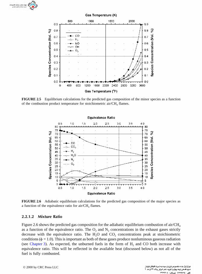
2.2.1.2 Mixture Ratio
Figure 2.6 shows the predicted gas composition for the adiabatic equilibrium combustion of air/CH4
as a function of the equivalence ratio. The O2 and N2 concentrations in the exhaust gases strictly decrease with the equivalence ratio. The H2O and CO2 concentrations peak at stoichiometric conditions (φ = 1.0). This is important as both of these gases produce nonluminous gaseous radiation (see Chapter 3). As expected, the unburned fuels in the form of H2 and CO both increase with equivalence ratio. This will be reflected in the available heat (discussed below) as not all of the fuel is fully combusted.
FIGURE 2.5 Equilibrium calculations for the predicted gas composition of the minor species as a function of the combustion product temperature for stoichiometric air/CH4 flames.
FIGURE 2.6 Adiabatic equilibrium calculations for the predicted gas composition of the major species as a function of the equivalence ratio for air/CH4 flames.
© 2000 by CRC Press LLC

2.2.1.3 Air and Fuel Preheat Temperature
In many industrial combustion processes, heat is recovered to improve the overall thermal efficiency of the process to reduce operating costs. The recovered heat is most commonly used to preheat the incoming combustion air and is sometimes used to preheat the incoming fuel. Preheating either the air or the fuel affects the composition of the combustion products. Figure 2.7 shows the major species predicted for the combustion of air and CH4 where the air is preheated up to as high as 2000°F (1366K). CO2, H2O, and N2 all decrease with air preheat, due to chemical dissociation. Figure 2.8 shows that the minor species increase with air preheat. Figures 2.9 and 2.10 show the
FIGURE 2.7 Adiabatic equilibrium stoichiometric calculations for the predicted gas composition of the major species as a function of the air preheat temperature for air/CH4 flames.
FIGURE 2.8 Adiabatic equilibrium stoichiometric calculations for the predicted gas composition of the minor species as a function of the air preheat temperature for air/CH4 flames.
© 2000 by CRC Press LLC

major and minor species, respectively, for air/CH4 flames as a function of the CH4 preheat temper-ature up to temperatures as high as 1000°F (811K). Due to safety considerations and the possibility of sooting up the fuel supply piping, higher fuel preheat temperatures are not practical or recom-mended under most conditions. The figures show that there is only a slight decrease in the concentrations of the major species and a slight increase in the concentrations of the minor species. This is due to the fact that the mass of fuel is relatively small compared to the mass of combustion air supplied to the system. This means that preheating the combustion air has a much more significant impact than preheating the fuel for a given preheat temperature.
FIGURE 2.9 Adiabatic equilibrium stoichiometric calculations for the predicted gas composition of the major species as a function of the fuel preheat for air/CH4 flames.
FIGURE 2.10 Adiabatic equilibrium stoichiometric calculations for the predicted gas composition of the minor species as a function of the fuel preheat for air/CH4 flames.
© 2000 by CRC Press LLC
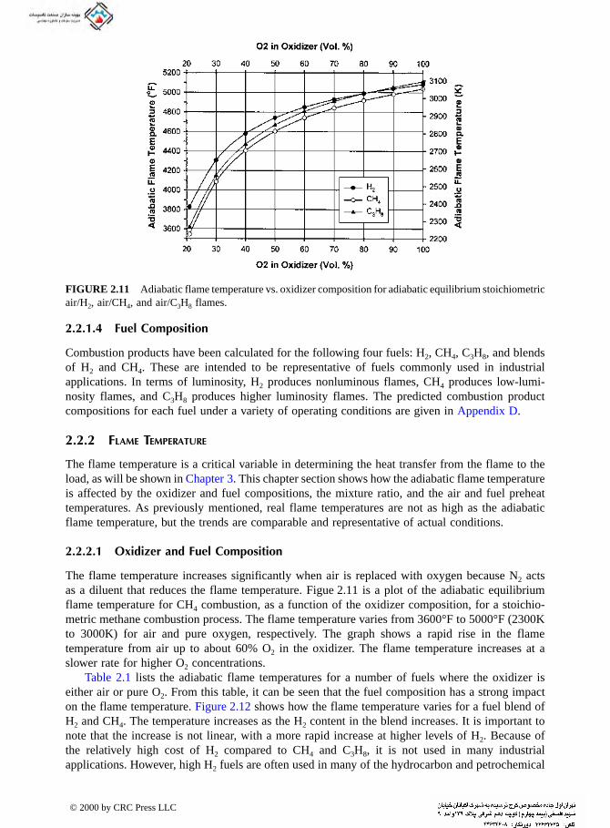
2.2.1.4 Fuel Composition
Combustion products have been calculated for the following four fuels: H2, CH4, C3H8, and blends of H2 and CH4. These are intended to be representative of fuels commonly used in industrial applications. In terms of luminosity, H2 produces nonluminous flames, CH4 produces low-lumi-nosity flames, and C3H8 produces higher luminosity flames. The predicted combustion product compositions for each fuel under a variety of operating conditions are given in Appendix D.
2.2.2 FLAME TEMPERATURE
The flame temperature is a critical variable in determining the heat transfer from the flame to the load, as will be shown in Chapter 3. This chapter section shows how the adiabatic flame temperature is affected by the oxidizer and fuel compositions, the mixture ratio, and the air and fuel preheat temperatures. As previously mentioned, real flame temperatures are not as high as the adiabatic flame temperature, but the trends are comparable and representative of actual conditions.
2.2.2.1 Oxidizer and Fuel Composition
The flame temperature increases significantly when air is replaced with oxygen because N2 acts as a diluent that reduces the flame temperature. Figue 2.11 is a plot of the adiabatic equilibrium flame temperature for CH4 combustion, as a function of the oxidizer composition, for a stoichio-metric methane combustion process. The flame temperature varies from 3600°F to 5000°F (2300K to 3000K) for air and pure oxygen, respectively. The graph shows a rapid rise in the flame temperature from air up to about 60% O2 in the oxidizer. The flame temperature increases at a slower rate for higher O2 concentrations.
Table 2.1 lists the adiabatic flame temperatures for a number of fuels where the oxidizer is either air or pure O2. From this table, it can be seen that the fuel composition has a strong impact on the flame temperature. Figure 2.12 shows how the flame temperature varies for a fuel blend of H2 and CH4. The temperature increases as the H2 content in the blend increases. It is important to note that the increase is not linear, with a more rapid increase at higher levels of H2. Because of the relatively high cost of H2 compared to CH4 and C3H8, it is not used in many industrial applications. However, high H2 fuels are often used in many of the hydrocarbon and petrochemical
FIGURE 2.11 Adiabatic flame temperature vs. oxidizer composition for adiabatic equilibrium stoichiometric air/H2, air/CH4, and air/C3H8 flames.
© 2000 by CRC Press LLC
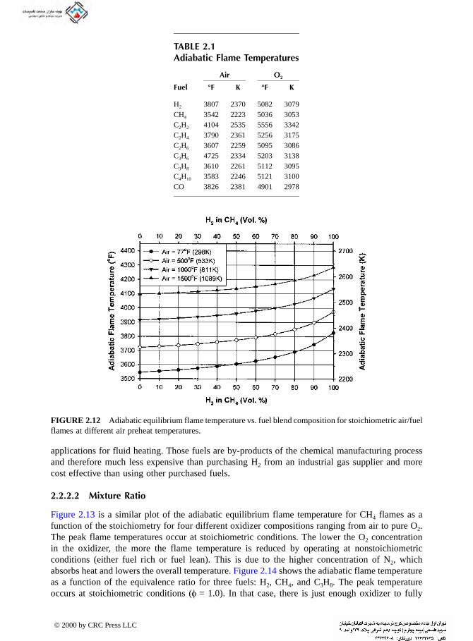
TABLE 2.1
applications for fluid heating. Those fuels are by-products of the chemical manufacturing process and therefore much less expensive than purchasing H2 from an industrial gas supplier and more cost effective than using other purchased fuels.
2.2.2.2 Mixture Ratio
Figure 2.13 is a similar plot of the adiabatic equilibrium flame temperature for CH4 flames as a function of the stoichiometry for four different oxidizer compositions ranging from air to pure O2. The peak flame temperatures occur at stoichiometric conditions. The lower the O2 concentration in the oxidizer, the more the flame temperature is reduced by operating at nonstoichiometric conditions (either fuel rich or fuel lean). This is due to the higher concentration of N2, which absorbs heat and lowers the overall temperature. Figure 2.14 shows the adiabatic flame temperature as a function of the equivalence ratio for three fuels: H2, CH4, and C3H8. The peak temperature occurs at stoichiometric conditions (φ = 1.0). In that case, there is just enough oxidizer to fully
Adiabatic Flame Temperatures
Air O2
Fuel °F K °F K
H2 3807 2370 5082 3079CH4 3542 2223 5036 3053C2H2 4104 2535 5556 3342C2H4 3790 2361 5256 3175C2H6 3607 2259 5095 3086C3H6 4725 2334 5203 3138C3H8 3610 2261 5112 3095C4H10 3583 2246 5121 3100CO 3826 2381 4901 2978
FIGURE 2.12 Adiabatic equilibrium flame temperature vs. fuel blend composition for stoichiometric air/fuel flames at different air preheat temperatures.
© 2000 by CRC Press LLC

combust all the fuel. Any additional oxidizer absorbs sensible energy from the flame and reduces the flame temperature. In most real flames, the peak flame temperature often occurs at slightly fuel-lean conditions (φ < 1.0). This is due to imperfect mixing where slightly more O2 is needed to fully combust all the fuel. Nearly all industrial combustion applications are run at fuel-lean conditions to ensure that the CO emissions are low. Therefore, depending on the actual burner design, the flame temperature may be close to its peak, which is often desirable for maximizing heat transfer. One problem often encountered when maximizing the flame temperature is that the NOx emissions are also maximized since NOx increases approximately exponentially with gas temperature. This has led to many design concepts for reducing the peak flame temperature in the flame to minimize NOx emissions.5 This also affects the heat transfer from the flame and is discussed in Chapters 3 and 8.
FIGURE 2.13 Adiabatic equilibirium flame temperature vs. stoichiometry for a CH4 flame and various oxidizers.
FIGURE 2.14 Adiabatic equilibrium flame temperature vs. equivalence ratio for air/H2, air/CH4, and air/C3H8 flames.
© 2000 by CRC Press LLC

2.2.2.3 Oxidizer and Fuel Preheat Temperature
Figure 2.15 shows how the adiabatic flame temperature varies as a function of the oxidizer preheat temperature for air/CH4 and O2 /CH4 flames. The increase in flame temperature is relatively small for the O2 /CH4 flame because the increased sensible heat of the O2 is only a fraction of the chemical energy contained in the fuel. For air/CH4 flames, preheating the air has a more dramatic impact because the increase in sensible heat is very significant due to the large mass of air in the combustion reaction. Figure 2.16 shows that the adiabatic flame temperature increases rapidly for air/fuel flames for each of the three fuels shown. Figure 2.12 also shows how preheating the air in the combustion of a blended fuel affects the flame temperature. Again, the higher the air preheat, the higher the temperature of the combustion products. Figure 2.17 shows that preheating the fuel has less impact on the flame temperature than preheating the oxidizer because of the mass flow rate differences, as previously discussed.
2.2.3 AVAILABLE HEAT
The available heat in a combustion system is important in determining the overall thermal efficiency and is therefore a factor when calculating the heat transfer in the process. It would be less effective to try to maximize the heat transfer in a system that inherently has a low available heat. Available heat is defined as the gross heating value of the fuel, less the energy carried out of the combustion process by the hot exhaust gases. The heat lost from a process through openings in the furnace, through the furnace walls, or by air infiltration are not considered in calculating the theoretical available heat as they are dependent on the process. The theoretical available heat should be proportional to the amount of energy actually absorbed by the load in an actual process, which is directly related to the thermal efficiency of the system. Therefore, the theoretical available heat is used here to show the thermal efficiency trends as functions of exhaust gas temperature, oxidizer and fuel compositions, mixture ratio, and air and fuel preheat temperatures.
FIGURE 2.15 Adiabatic equilibrium flame temperature vs. oxidizer preheat temperature for stoichiometric air/CH4 and O2 /CH4 flames.
© 2000 by CRC Press LLC

Figure 2.18 shows how the available heat decreases rapidly with the exhaust gas temperature and is relatively independent of the fuel composition for the three fuels shown. Then, to maximize the thermal efficiency of a process, it is desirable to minimize the exhaust gas temperature. This is usually done by maximizing the heat transfer from the exhaust gases to the load (and furnace walls) and by recovering some of the heat in the exhaust gases by preheating the fuel and/or the oxidizer. Figure 2.19 shows how the available heat, for stoichiometric air/CH4 and O2 /CH4 flames, varies as a function of the exhaust gas temperature. As the exhaust temperature increases, more energy is carried out of the combustion system and less remains in the system. The available heat decreases to zero at the adiabatic equilibrium flame temperature where no heat is lost from the gases. The figure shows that even at gas temperatures as high as 3500°F (2200K), the available
FIGURE 2.16 Adiabatic equilibrium flame temperature vs. air preheat temperature for stoichiometric air/H2, air/CH4, and air/C3H8 flames.
FIGURE 2.17 Adiabatic equilibrium flame temperature vs. fuel preheat temperature for stoichiometric air/H2, air/CH4, and air/C3H8 flames.
© 2000 by CRC Press LLC

heat of an O2 /CH4 system is still as high as 57%. The figure also shows that it is usually not very economical to use air/CH4 systems for high-temperature heating and melting processes. At an exhaust temperature of 2500°F (1600K), the available heat for the air/CH4 system is only a little over 30%. Heat recovery in the form of preheated air is commonly used for higher temperature heating processes to increase the thermal efficiencies.
Figure 2.20 is a graph of the available heat for the combustion of CH4 as a function of the O2
concentration in the oxidizer, for three different exhaust gas temperatures. As the exhaust gas
FIGURE 2.18 Available heat vs. gas temperature for stoichiometric air/H2, air/CH4, and air/C3H8 flames.
FIGURE 2.19 Available heat vs. exhaust gas temperature for stoichiometric air/CH4 and O2 /CH4 flames.
© 2000 by CRC Press LLC

temperature increases, the available heat decreases because more energy is carried out the exhaust stack. There is an initial rapid increase in available heat as the O2 concentration in the oxidizer increases from the 21% found in air. That is one reason why O2 enrichment has been a popular technique for using OEC because the incremental increase in efficiency is very significant.
Figure 2.21 shows how the available heat increases with the oxidizer preheat temperature. The thermal efficiency of the air/CH4 doubles by preheating the air to 2000°F (1400K). For the O2 /CH4
flames, the increase in efficiency is much less dramatic by preheating the O2. This is because the initial efficiency with no preheat is already 70% and because the mass of the O2 is not nearly as significant in the combustion reaction as compared to the mass of air in an air/fuel flame. There are also safety concerns when flowing hot O2 through piping, heat recuperation equipment, and a burner. Figure 2.22 shows that the available heat increases rapidly for any of the three fuels shown as the combustion air preheat temperature increases.
The fuel savings for a given technology can be calculated using the available heat curves:
(2.23)
where AH1 is the available heat of the base case process and AH2 is the available heat using a new technology. For example, if the base case process has an available heat of 30% and the available heat using the new technology is 45%, then the fuel savings equal (1 – 45/30) × 100 = –50%, which means that 50% less fuel is needed for process 2 compared to process 1.
2.2.4 FLUE GAS VOLUME
The flow rate of gases through a combustion chamber is proportional to the convective heat transfer to the load. There are several factors that influence this flow rate. One is the gas temperature since
FIGURE 2.20 Available heat vs. oxidizer composition for a stoichiometric CH4 flame, at exhaust temper-atures of 2000°F, 2500°F, and 3000°F.
Fuel savings %( ) = −⎛⎝⎜
⎞⎠⎟
×1 1002
1
AH
AH
© 2000 by CRC Press LLC

higher temperature gases have higher actual flow rates (e.g., actual cubic feet per hour or ACFH) due to the thermal expansion of the gases. This means that preheating the fuel or the oxidizer, which both normally increase the flame temperature, would produce higher actual flow rates. However, the flow rate of the gases is the same when corrected to standard temperature and pressure conditions (STP). Another factor that has a very strong influence on the gas flow rate through the combustion system is the oxidizer composition. Oxygen-enhanced combustion basically involves
FIGURE 2.21 Available heat vs. oxidizer preheat temperature for equilibrium stoichiometric air/CH4 and O2 /CH4 flames at an exhaust gas temperature of 2500°F (1644K).
FIGURE 2.22 Available heat vs. air preheat temperature for equilibrium stoichiometric air/H2, air/CH4, and air/C3H8 flames at an exhaust gas temperature of 2000°F (1366K).
© 2000 by CRC Press LLC
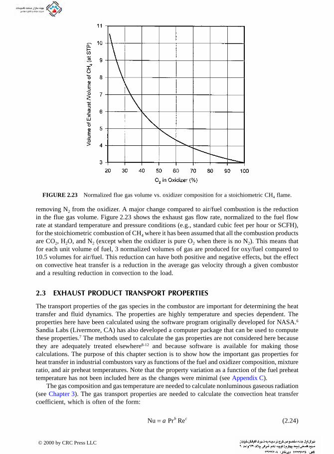
removing N2 from the oxidizer. A major change compared to air/fuel combustion is the reduction in the flue gas volume. Figure 2.23 shows the exhaust gas flow rate, normalized to the fuel flow rate at standard temperature and pressure conditions (e.g., standard cubic feet per hour or SCFH), for the stoichiometric combustion of CH4 where it has been assumed that all the combustion products are CO2, H2O, and N2 (except when the oxidizer is pure O2 when there is no N2). This means that for each unit volume of fuel, 3 normalized volumes of gas are produced for oxy/fuel compared to 10.5 volumes for air/fuel. This reduction can have both positive and negative effects, but the effect on convective heat transfer is a reduction in the average gas velocity through a given combustor and a resulting reduction in convection to the load.
2.3 EXHAUST PRODUCT TRANSPORT PROPERTIES
The transport properties of the gas species in the combustor are important for determining the heat transfer and fluid dynamics. The properties are highly temperature and species dependent. The properties here have been calculated using the software program originally developed for NASA.6
Sandia Labs (Livermore, CA) has also developed a computer package that can be used to compute these properties.7 The methods used to calculate the gas properties are not considered here because they are adequately treated elsewhere8-12 and because software is available for making those calculations. The purpose of this chapter section is to show how the important gas properties for heat transfer in industrial combustors vary as functions of the fuel and oxidizer composition, mixture ratio, and air preheat temperatures. Note that the property variation as a function of the fuel preheat temperature has not been included here as the changes were minimal (see Appendix C).
The gas composition and gas temperature are needed to calculate nonluminous gaseous radiation (see Chapter 3). The gas transport properties are needed to calculate the convection heat transfer coefficient, which is often of the form:
(2.24)
FIGURE 2.23 Normalized flue gas volume vs. oxidizer composition for a stoichiometric CH4 flame.
Nu = a b cPr Re
© 2000 by CRC Press LLC

where the Nu is the Nusselt number, Pr is the Prandtl number, Re is the Reynolds number, and a, b, and c are constants. The constants depend on the flow conditions, but often b Ý 1/3 and c Ý
2/3. The convection heat transfer coefficient h is then calculated from the Nusselt number using:
(2.25)
where d is a characteristic dimension for the flow system and k is the fluid thermal conductivity. The gas properties are needed to calculate the Nusselt, Prandtl, and Reynolds numbers, as will be shown next.
2.3.1 DENSITY
The gas density (ρ) can be used to calculate the Reynolds number (Re = ρv d/µ), which is usually needed to compute the convective heat transfer coefficient (h), which is discussed in the Chapter 3. The density is also used to calculate the average gas velocity through the combustor, which is also usually needed to compute the convection coefficient:
(2.26)
where •
m is the mass flow rate of gases (which is known and equal to the sum of the incoming fuel + oxidizer flow rates) and A is the cross-sectional area of the combustor. The gas density is inversely proportional to the gas temperature so that as the temperature increases, the density decreases.
Figure 2.24 shows that the gas density declines approximately proportional to the inverse of the absolute gas temperature. Figure 2.25 shows how the gas density decreases rapidly as the O2
content in the oxidizer increases, for all three fuels shown. This is a consequence of the increased flame temperatures, as shown in Figure 2.11. A lower gas density means a lower Reynolds number and therefore reduced convective heat transfer, if all other variables remain the same. However, the mass flow rate of gases is also decreasing, as shown in Figure 2.23. Therefore, the average gas
FIGURE 2.24 Calculated gas density for equilibrium stoichiometric flames as a function of the combustion product temperature and fuel composition.
Nu = hdk
vmA
=˙
ρ
© 2000 by CRC Press LLC
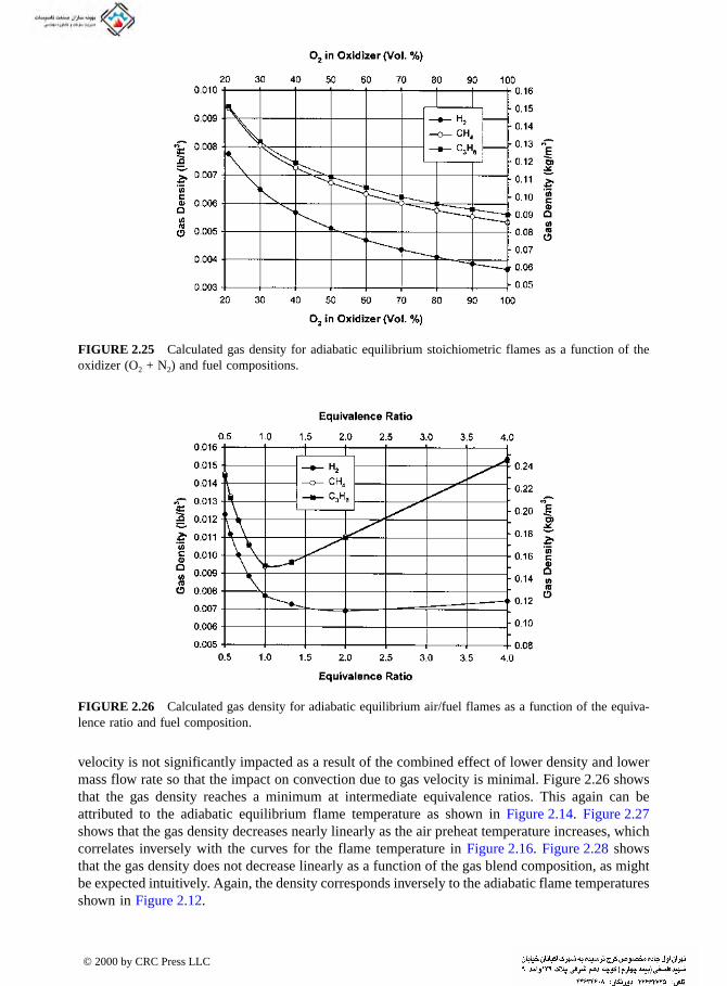
velocity is not significantly impacted as a result of the combined effect of lower density and lower mass flow rate so that the impact on convection due to gas velocity is minimal. Figure 2.26 shows that the gas density reaches a minimum at intermediate equivalence ratios. This again can be attributed to the adiabatic equilibrium flame temperature as shown in Figure 2.14. Figure 2.27 shows that the gas density decreases nearly linearly as the air preheat temperature increases, which correlates inversely with the curves for the flame temperature in Figure 2.16. Figure 2.28 shows that the gas density does not decrease linearly as a function of the gas blend composition, as might be expected intuitively. Again, the density corresponds inversely to the adiabatic flame temperatures shown in Figure 2.12.
FIGURE 2.25 Calculated gas density for adiabatic equilibrium stoichiometric flames as a function of the oxidizer (O2 + N2) and fuel compositions.
FIGURE 2.26 Calculated gas density for adiabatic equilibrium air/fuel flames as a function of the equiva-lence ratio and fuel composition.
© 2000 by CRC Press LLC

2.3.2 SPECIFIC HEAT
The gas specific heat (cp), sometimes referred to as the gas heat capacity, is another transport property that has an impact on the convective heat transfer in a system. It is used to calculate the Prandtl number (Pr = cp µ/k), which is often used to calculate the convective heat transfer coefficient (h).
Figure 2.29 shows a nonlinear increase in the gas specific heat as a function of the exhaust product temperature. The specific heat increases more rapidly at higher temperatures. Figure 2.30 shows that the exhaust gas specific heat increases almost linearly as the O2 purity in the oxidizer increases for all three fuels considered. All other things being the same, this would enhance the convective heat transfer from the combustion product gases to the load. Figure 2.31 shows a much more complicated relationship between the specific heat and the equivalence ratio, including a strong fuel dependence as well. All three fuels show an initial increase in the specific heat as the
FIGURE 2.27 Calculated gas density for adiabatic equilibrium stoichiometric air/fuel flames as a function of the air preheat temperature and fuel composition.
FIGURE 2.28 Calculated gas density for adiabatic equilibrium stoichiometric air/fuel flames as a function of the fuel blend composition and air preheat temperature.
© 2000 by CRC Press LLC

equivalence ratio increases, reaching a local maximum at stoichiometric conditions (φ = 1.0). Beyond stoichiometric conditions, the specific heat then decreases, plateaus, and increases again. In the case of CH4, the specific heat increases very rapidly at high equivalence values. Although the relationship between specific heat and equivalence ratio is fairly complicated, the reality is that most industrial combustion processes are operated at slightly fuel-lean conditions where there is a strong but more linear relationship between the equivalence ratio and the specific heat. Figure 2.32 shows an almost linear dependence of specific heat on air preheat temperature for all three fuels. Figure 2.33 shows that the specific heat increases rapidly at high H2 contents in H2 /CH4 fuel blends. Intuitively, one might expect a linear relationship; but as can be seen in, the flame temperature shows a very similar relationship to the H2 content in the blend.
FIGURE 2.29 Calculated gas specific heat for equilibirium stoichiometric flames as a function of the combustion product temperature and fuel composition.
FIGURE 2.30 Calculated gas specific heat for adiabatic equilibrium stoichiometric flames as a function of the oxidizer (O2 + N2) and fuel compositions.
© 2000 by CRC Press LLC
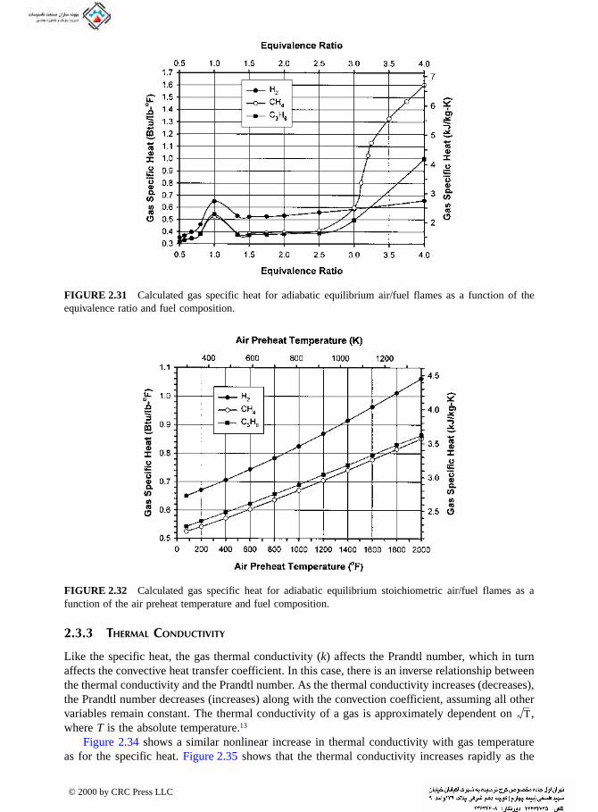
2.3.3 THERMAL CONDUCTIVITY
Like the specific heat, the gas thermal conductivity (k) affects the Prandtl number, which in turn affects the convective heat transfer coefficient. In this case, there is an inverse relationship between the thermal conductivity and the Prandtl number. As the thermal conductivity increases (decreases), the Prandtl number decreases (increases) along with the convection coefficient, assuming all othervariables remain constant. The thermal conductivity of a gas is approximately dependent on , where T is the absolute temperature.13
Figure 2.34 shows a similar nonlinear increase in thermal conductivity with gas temperature as for the specific heat. Figure 2.35 shows that the thermal conductivity increases rapidly as the
FIGURE 2.31 Calculated gas specific heat for adiabatic equilibrium air/fuel flames as a function of the equivalence ratio and fuel composition.
FIGURE 2.32 Calculated gas specific heat for adiabatic equilibrium stoichiometric air/fuel flames as a function of the air preheat temperature and fuel composition.
T
© 2000 by CRC Press LLC

O2 content in the oxidizer increases. The relationship is almost linear although there is a faster increase at lower O2 contents compared to that at higher O2 oxidizers. Figure 2.36 again shows a complicated relationship between a transport property and the equivalence ratio. There is a local maxima at stoichiometric conditions (φ = 1.0). For H2, the local maxima also is the overall maximum for the range of equivalence ratios computed. For CH4, there is a rapid increase in the thermal conductivity at very fuel-rich conditions (high equivalence ratios), with the conductivity exceeding the local maxima at stoichiometric conditions. Although not as dramatic, there is a similar phe-nomenon for C3H8. Although most industrial processes are run at slightly fuel-lean conditions, there is still a rapid change in thermal conductivity on the fuel-lean side of stoichiometric conditions. Figure 2.37 shows a much simpler relationship between conductivity and combustion air preheat temperature. The conductivity increases slightly faster than linearly as the preheat temperature
FIGURE 2.33 Calculated gas specific heat for adiabatic equilibrium stoichiometric air/fuel flames as a function of the fuel blend composition and air preheat temperature.
FIGURE 2.34 Calculated gas thermal conductivity for equilibrium stoichiometric flames as a function of the combustion product temperature and fuel composition.
© 2000 by CRC Press LLC

increases. As previously shown for other transport properties, Figure 2.38 shows that the thermal conductivity increases much more rapidly as the H2 content in the H2 /CH4 fuel blend increases.
2.3.4 VISCOSITY
The absolute or dynamic viscosity µ is a measure of momentum diffusion. Gas viscosity has a similar relationship to as does thermal conductivity.13 The viscosity is important in calculating both the Prandtl and Reynolds numbers, but in opposite ways. As the gas viscosity increases (decreases), the Prandtl number increases (decreases) and the Reynolds number decreases (increases), assuming all other variables are constant. The kinematic viscosity ν is related to the dynamic viscosity as follows:
FIGURE 2.35 Calculated gas thermal conductivity for adiabatic equilibrium stoichiometric flames as a function of the oxidizer (O2 + N2) and fuel compositions.
FIGURE 2.36 Calculated gas thermal conductivity for adiabatic equilibrium air/fuel flames as a function of the equivalence ratio and fuel composition.
T
© 2000 by CRC Press LLC

(2.27)
and is sometimes used to define the Reynolds number:
(2.28)
where v is the fluid velocity and d is some characteristic dimension for the system under investigation.
FIGURE 2.37 Calculated gas thermal conductivity for adiabatic equilibrium stoichiometric air/fuel flames as a function of the air preheat temperature and fuel composition.
FIGURE 2.38 Calculated gas thermal conductivity for adiabatic equilibrium stoichiometric air/fuel flames as a function of the fuel blend composition and air preheat temperature.
νρ
= µ
Re = vdν
© 2000 by CRC Press LLC

Figure 2.39 shows a nearly linear increase in gas viscosity as a function of the exhaust product temperature. Figure 2.40 shows that the gas viscosity increases as the O2 content in the oxidizer increases, similar to the adiabatic flame temperature as shown in Figure 2.11. Figure 2.41 shows that the gas viscosity peaks at an equivalence ratio of 1.0 (stoichiometric conditions) and declines as the mixture becomes either more fuel rich or more fuel lean. Again, this compares to the adiabatic flame temperature as a function of equivalence ratio as shown in Figure 2.14. As shown in Figure 2.42, the gas viscosity increases with the air preheat temperature, comparable to the flame temperature as shown in Figure 2.16. Figure 2.43 shows that the viscosity increases as the H2
content increases in an H2 /CH4 fuel blend. Just as for the adiabatic flame temperature shown in, the viscosity increases more rapidly at higher H2 contents.
FIGURE 2.39 Calculated gas viscosity for equilibrium stoichiometric flames as a function of the combustion product temperature and fuel composition.
FIGURE 2.40 Calculated gas viscosity for adiabatic equilibrium stoichiometric flames as a function of the oxidizer (O2 + N2) and fuel compositions.
© 2000 by CRC Press LLC

2.3.5 PRANDTL NUMBER
As was previously shown, the Prandtl number is often used to calculate the convection heat transfer coefficient. The components of Pr, including the specific heat, viscosity, and thermal conductivity, were discussed above. This chapter section shows how the combination of these variables which forms the Prandtl number changes as functions of the fuel and oxidizer compositions, the mixture ratio, and the air preheat temperature. Since there is little change in Pr as a function of the fuel preheat temperature, that is not included here but the data are given in Appendix D.
Figure 2.44 shows that the Prandtl number decreases as a function of temperature, but in a nonuniform way. Initially, it decreases moderately quickly, then decreases more slowly, and finally
FIGURE 2.41 Calculated gas viscosity for adiabatic equilibrium air/fuel flames as a function of the equiv-alence ratio and fuel composition.
FIGURE 2.42 Calculated gas viscosity for adiabatic equilibrium stoichiometric air/fuel flames as a function of the air preheat temperature and fuel composition.
© 2000 by CRC Press LLC

decreases rapidly at higher temperatures. Figure 2.45 also shows a highly nonlinear relationship between the Prandtl number and the oxidizer composition. For CH4 and C3H8, the Prandtl numberdecreases rapidly at first and then levels off at higher O2 contents. For H2, the Prandtl number actually has a minima at about 50% O2 content. Figure 2.46 shows a highly nonlinear relationship between the Prandtl number and the equivalence ratio. All three fuels show local maxima and minima at 1.0 < φ < 2.0. In Figure 2.47, the Prandtl number declines almost linearly with the air preheat temperature. Figure 2.48 shows that the Prandtl number declines as the H2 content in an H2 /CH4 fuel blend decreases, and decreases rapidly at high H2 contents.
FIGURE 2.43 Calculated gas viscosity for adiabatic equilibrium stoichiometric air/fuel flames as a function of the fuel blend composition and air preheat temperature.
FIGURE 2.44 Calculated Prandtl number for equilibrium stoichiometric flames as a function of the com-bustion product temperature and fuel composition.
© 2000 by CRC Press LLC

2.3.6 LEWIS NUMBER
The Lewis number is the ratio of the thermal diffusivity to the molecular (mass) diffusivity and is defined as:
(2.29)
where D is the mass diffusivity for the fluid. The importance of the Lewis number to heat transfer in combustion systems is considered in more detail in Chapter 4. In general, for Le > 1, there are some enhancements in convective heat transfer due to chemical recombination reactions.
FIGURE 2.45 Calculated Prandtl number for adiabatic equilibrium stoichiometric flames as a function of the oxidizer (O2 + N2) and fuel compositions.
FIGURE 2.46 Calculated Prandtl number for adiabatic equilibrium air/fuel flames as a function of the equivalence ratio and fuel composition.
Le =k c
Dpρ
© 2000 by CRC Press LLC

Figure 2.49 shows that the Lewis number is 1 for temperatures below about 2300°F (1500K), depending on the fuel, and then rises fairly rapidly at higher temperatures. Figure 2.50 shows that the Lewis number is greater than unity for all oxidizer compositions under adiabatic equilibrium conditions, which equates to the highest flame temperature possible for those conditions. The shape of the curves is interesting in that Le peaks at intermediate oxidizer compositions and actually declines at higher O2 contents. Figure 2.51 shows a dramatic peak in the Lewis number at stoichi-ometric conditions, with the Lewis number actually going below 1.0 at higher equivalence ratios. Figure 2.52 shows that the Lewis number increases almost linearly with the air preheat temperature for adiabatic equilibrium conditions. The Lewis number increases more rapidly as the H2 content in a fuel blend of H2 /CH4 increases, as shown in Figure 2.53.
FIGURE 2.47 Calculated Prandtl number for adiabatic equilibrium stoichiometric air/fuel flames as a function of the air preheat temperature and fuel composition.
FIGURE 2.48 Calculated Prandtl number for adiabatic equilibrium stoichiometric air/fuel flames as a function of the fuel blend composition and air preheat temperature.
© 2000 by CRC Press LLC

FIGURE 2.49 Calculated Lewis number for equilibrium stoichiometric flames as a function of the combus-tion product temperature and fuel composition.
FIGURE 2.50 Calculated Lewis number for adiabatic equilibrium stoichiometric flames as a function of the oxidizer (O2 + N2) and fuel compositions.
© 2000 by CRC Press LLC

FIGURE 2.51 Calculated Lewis number for adiabatic equilibrium air/fuel flames as a function of the equivalence ratio and fuel composition.
FIGURE 2.52 Calculated Lewis number for adiabatic equilibrium stoichiometric air/fuel flames as a function of the air preheat temperature and fuel composition.
© 2000 by CRC Press LLC

REFERENCES
1. C. Baukal, Ed., Oxygen-Enhanced Combustion, CRC Press, Boca Raton, FL, 1998.2. A.I. Dalton and D.W. Tyndall, Oxygen Enriched Air/Natural Gas Burner System Development, NTIS
Report PB91-167510, Springfield, VA, 1989.3. I. Glassman, Combustion, 3rd edition, Academic Press, New York, 1996.4. S. Gordon and B.J. McBride, Computer Program for Calculation of Complex Chemical Equilibrium
Compositions, Rocket Performance, Incident and Reflected Shocks, and Chapman-Jouguet Detona-tions, NASA Report SP-273, 1971.
5. J.L. Reese, G.L. Moilanen, R. Borkowicz, C. Baukal, D. Czerniak, and R. Batten, State-of-the-Art of NOx emission control technology, ASME Paper 94-JPGC-EC-15, Proceedings of Int. Joint Power Generation Conf., Phoenix, AZ, 3-5 October, 1994.
6. S. Gordon, B.J. McBride, and F.J. Zeleznik, Computer Program for Calculation of Complex Chemical Equilibrium Compositions and Applications. Supplement I. Transport Properties, NASA Technical Memorandum 86885, Washington, D.C., 1984.
7. R.J. Kee, G. Dixon-Lewis, J. Warnatz, M.E. Coltrin, and J.A. Miller, A Fortran Computer Package for the Evaluation of Gas-Phase, Multicomponent Transport Properties, Sandia National Laboratory Report SAND86-8246, Livermore, CA, 1986.
8. R.B. Bird, W.E. Stewart, and E.N. Lightfoot, Transport Phenomena, Wiley, New York, 1960.9. N.V. Tsederberg, Thermal Conductivity of Gases and Liquids, MIT Press, Cambridge, MA, 1965.
10. P.E. Liley, R.C. Reid, and E. Buck, Physical and Chemical Data, Section 3 in Perry’s Chemical Engineers’ Handbook, 6th edition, R.H. Perry and D. Green, Eds., McGraw-Hill, New York, 1984.
11. R.C. Reid, J.M. Prausnitz, and B.E. Poling, The Properties of Gases and Liquids, 4th edition, McGraw-Hill, New York, 1987.
12. D.R. Lide, Ed., CRC Handbook of Chemistry and Physics, 79th edition, CRC Press, Boca Raton, FL, 1998.
13. B. Gebhart, Heat Transfer, 2nd edition, McGraw-Hill, New York, 1971.
FIGURE 2.53 Calculated Lewis number for adiabatic equilibrium stoichiometric air/fuel flames as a function of the fuel blend composition and air preheat temperature.
© 2000 by CRC Press LLC

Heat Transfer Modes
0-8493-7686-6/97/$0.00+$.50© 1997 by CRC Press LLC
33.1 INTRODUCTION
There are some nondimensional numbers that are commonly used in heat transfer analysis. The Reynolds number (Re) is the ratio of the inertial forces to the viscous forces in a flow:
(3.1)
where ρ is the fluid density, v is the fluid velocity, l is the characteristic length scale (e.g., diameter for a pipe for flow through a pipe), µ is the absolute viscosity, and ν is the kinematic viscosity. The Reynolds number is low for laminar flows and high for turbulent flows, with transition flow at values in between. The actual range for each type of flow depends on the flow geometry. The Prandtl number (Pr) is the ratio of momentum diffusivity to thermal diffusivity and is defined as:
(3.2)
where cp is the fluid constant pressure specific heat and k is the fluid thermal conductivity. For many gases, Pr Ý 0.7. The Nusselt number (Nu) is the ratio of the convective and conductive heat transfer rates:
(3.3)
where h is the convective heat transfer coefficient. In forced convection flows, Nu is commonly a function of Pr and Re and is used to determine the convection coefficient.
3.2 CONVECTION
Convection heat transfer is caused by fluid motion past a material, where the fluid is either at a higher or lower temperature than the material. In industrial combustion applications, the fluid is usually at a higher temperature than the medium it is heating. At least one person has argued that convection is not actually a separate mode of heat transfer, but that it is a subset of conduction because the energy must still conduct from the fluid to the material.1 While that may true on a microscopic scale in the boundary layer next to the material, convection is a fundamentally different process from conduction and is treated here as such, which is the convention in standard heat transfer texts. Forced convection is often a very important mode of heat transfer in industrial combustion systems. In limited applications, natural convection may also be important because of high-temperature gradients that may exist. Forced and natural convection may be important in industrial combustion and are briefly considered next. A cartoon of forced and natural convection is shown in Figure 7.3. A number of books are available specifically on convection heat transfer.2-10
Re =µ=ρν
vl vl
Pr =µc
kp
Nu = hlk
© 2000 by CRC Press LLC

3.2.1 FORCED CONVECTION
Forced convection heat transfer occurs when a fluid is forcefully directed at or over a medium
(liquid or solid) and may be simply calculated using:
(3.4)
where q is the heat flux to the medium (Btu/hr or kW), h is the convective heat transfer coefficient (Btu/ft2-hr-°F or W/m2-K), A is the surface area of the medium in contact with the moving fluid, tf is the fluid temperature (°F or K), and tm is the temperature (°F or K) of the medium. A simple example is given below.
Example 3.1
Given: h = 10 Btu/ft2-hr-°F, A = 10 ft2, tf = 300°F, and tm = 70°F.
Find: q
Solution: q = h A (tm – tf) = (10 Btu/ft2-hr-°F)(10 ft2)(300°F – 70°F) = 23,000 Btu/hr
This is an overly simplified example because the convection heat transfer coefficient, h, has been given. In most problems, this value must be calculated from an appropriate correlation which may be fairly complicated, or worse, may not exist for the exact configuration under study. In the latter case, either experiments need to be done to determine this value or an approximate value must be used. The correlations for the convection coefficient are often complicated functions that normally depend on the flow geometry, the fluid velocity, and the fluid properties. In addition, for most real problems, the fluid and medium temperatures vary by location and are not constant over the entire medium surface. Forced convection heat transfer from a flame to the load and inner combustor walls and from the outer combustor walls to the ambient are both potentially important mechanisms. Forced convection heat transfer in industrial combustion is often more difficult to analyze and calculate because of the large temperature difference between the combustion products and the surfaces (furnace walls and heat load) and because the gas properties vary widely as a function of both temperature and composition (see Chapter 2).
3.2.1.1 Forced Convection from Flames
In many conventional furnace heating processes, forced convection is only a small fraction of the total heat transfer to the product. Most of the heating emanates from the radiation from the hot refractory walls. However, in flame impingement, with no furnace enclosure, forced convection may be 70% to 90% of the total heat flux.11,12 For flame temperatures up to about 2600°F (1700K), forced convection is the dominant mechanism in flame impingement heat transfer.13
For low-temperature flames, as is common in air/fuel combustion systems, forced convection has generally been the only mechanism considered. In highly dissociated oxygen/fuel flames, a large fraction of the heat release is from exothermic reactions. However, even for those flames, forced convection is still an important contributor to the overall heat transfer to the target.
The turbulence level directly affects the importance of forced convection. The flow regime is determined by the Reynolds number, defined in Equation 3.1. For example, for flame jet impinge-ment (see Figure 3.1) there are many possible choices for the length l. One is the burner outlet nozzle diameter, dn; another is the axial distance from the nozzle exit to the surface being heated, lj; a third possibility is the width of the jet at the edge of the stagnation zone, dj; still another is some dimension of the material being heated. For a disk or cylinder, it may be the diameter, db. For a plane surface, it may be the radial distance from the stagnation point, r. In one case, the width of the water cooling channel in a target used in a flame impingement study was used.13
q hA t tf m= −( )
© 2000 by CRC Press LLC

Laminar flames have been used in many flame impingement studies.13-23 Sibulkin developed a semianalytical solution for the heat transfer for laminar flow, normal to the stagnation point of an axisymmetric, blunt-nosed target:24
(3.5)
This result has been the basis for all other semianalytical flame impingement heat transfer solutions.25
Turbulent flames have also been commonly used.12,26-38 A typical example of an empirical equation, incorporating the turbulence intensity Tu, was given by Hustad37 as
(3.6)
This was developed for flames produced by jets of CH4 and C3H8, into ambient air. These are known as pure diffusion (φ = ×) flames. The flames impinged normal to uncooled steel pipes. These experiments were done to simulate fires caused by ruptured fuel pipes in the petrochemical industry. Similar empirical correlations are discussed further in Chapter 7.
Babiy (1974) presented a correlation for the convective heat transfer from combustion gases to carbon particles in pulverized coal combustion processes.39 A commonly used equation for the convective heat transfer between a gas and a sphere is given by:
(3.7)
where d is the diameter of the sphere. For pulverized coal combustion, this equation is modified as follows:
(3.8)
where Tg is the absolute temperature of the gas (K). The equation applies for Tg = 1200–1600K (1700–2400°F), O2 = 5–21%, d = 150–1000 µm, and Red < 1.
FIGURE 3.1 Flame jet impingement.
′′= µ( ) −( )−q c t ts s e e e p e we0 763
0 5 0 6. Pr. .β ρ
′′=⎛⎝⎜
⎞⎠⎟
⎧⎨⎪
⎩⎪
⎫⎬⎪
⎭⎪−( )q
k
dt ts
e
bb,e e
e
we w0 41 0 6 0 35 0 15
0 25
. Re PrPr
Pr. . .
.
Tu
Nud d= +2 0 17 0 66. Re .
Nu Nud dgT
* exp= −⎛
⎝⎜
⎞
⎠⎟
⎡
⎣⎢⎢
⎤
⎦⎥⎥
1455000
© 2000 by CRC Press LLC
3.2.1.2 Forced Convection from Outside Combustor Wall
The second place where forced convection is often important is where heat is transferred from the
hot shell of a combustor to the cooler ambient air. Griswold (1946)40 has recommended the following empirical correlation for the natural convection coefficient for wind flowing against a surface:
(3.9)
where hc = convection coefficient (Btu/hr-ft2-°F), v = air velocity, direction unspecified (ft/sec), tw = outside wall temperature (°F), and t× = ambient air temperature (°F).
3.2.1.3 Forced Convection from Hot Gases to Tubes
In the convection section of a heater, Monrad (1932)41 recommended the following empirical correlation for the convective heat transfer from hot exhaust products to a bank of staggered tubes:
(3.10)
where hc = convection coefficient (Btu/hr-ft2-°F), G = gas mass velocity at minimum free cross-sectional area (lb/ft2-sec), Tg = absolute gas temperature (°R), and d = tube diameter (in.).
3.2.2 NATURAL CONVECTION
Natural convection is sometimes referred to as buoyancy-induced flow.42 There are two common situations where natural convection heat transfer may be important in industrial combustion systems. The first is transferring heat from the flame in a system where the gas velocities are very low. The second is transferring heat from the outside shell of a combustor to the environment. Each is briefly considered next.
3.2.2.1 Natural Convection from Flames
One measure of the intensity of natural convection is the Rayleigh number:
(3.11)
which is analogous to the Reynolds number for forced convection. Higher Rayleigh numbers indicate more natural convection. Another measure of intensity is the Grashoff number:
(3.12)
where g is the gravity constant, β∼
is the volume coefficient of expansion (= 1/T for an ideal gas), and ν is the kinematic viscosity. The Richardson number, Ri, is one measure of the importance of buoyancy compared to forced convection. It is defined as:
(3.13)
hv
t tcw
= +−( )∞
1 0 225.
hG T
dcg=
1 6 2 3 0 3
1 3
. .
Ra =g q l
ce f j
e p ee
βρ ν
2
3
Gr =−( )∞g t t lwβν
3
2
RiGr=Ren
2
© 2000 by CRC Press LLC

which is the ratio of the buoyant force to the inertial force. Conolly and Davies (1972) studied stoichiometric, laminar flames impinging on a hemi-nosed cylinder.19 The flame was parallel to
the cylinder and impinging on the nose. A variety of fuels and oxidizers were used. Buoyancy effects were negligible. The criterion was that buoyancy may be neglected, compared to forced convection, for Ri < 0.05. Wang (1993) numerically modeled a nonreacting jet of ambient air, impinging on an infinite flat plate.43 It was concluded that natural convection is important only when Rej is low, and the temperature difference between the jet and the stagnation surface is large. The critical Ri was estimated to be approximately 0.02. You (1985)23 determined the heat transfer from a buoyant flame to a flat plate in terms of the Rayleigh number as
(3.14)
The flames were produced by upward jets of pure natural gas (φ = ×) into ambient air. The jets impinged on a horizontal surface to simulate a fire spreading over the ceiling of a room. Natural convection is more important in low-velocity flames. Both Beér (1968)11 and Vizioz (1971)27 stated that the effects of buoyancy were negligible in their studies, due to the high burner exit velocities.
3.2.2.2 Natural Convection from Outside Combustor Wall
The second place where natural convection is often important is where heat is transferred from the hot shell of a combustor to the cooler ambient air. Griswold40 has recommended the following empirical correlation for the natural convection coefficient for quiet air:
(3.15)
where hc = convection coefficient (Btu/hr-ft2-°F), C = shape constant (1.39 for a vertical wall or 1.79 for a furnace arch), Tw = outside wall temperature (°R), and T× = ambient air temperature (°R).
Example 3.2
Given: tw = 150°F, t× = 70°F.
Find: Average heat loss per unit area by natural convection from a vertical surface using the above equation.
Solution: q″= hc (tw – t×) = = 83 Btu/hr-ft2
3.3 RADIATION
Thermal radiation is one of the most important heat transfer mechanisms in industrial furnaces.44
Radiation is a unique method of heat transfer as no medium is required for energy transport — it can be transmitted through a vacuum or through a medium. Radiation is simply the transmission of energy by electromagnetic waves, which are characterized by their wavelength or frequency and are related as follows:
(3.16)
′′ = ( ) − −q q lb f j e e31 2 2 1 6 3 5. PrRa
hC T T
T Tc
w
w
=−( )
+( )[ ]∞
∞
0 53
2
0 27
0 18
..
.
0 53 1 39 150 460 70 460
150 460 70 460 2150 70
0 27
0 18
. . .
.
( ) +( ) − +( )[ ]+( ) + +( )[ ]
−( )
λν= c
© 2000 by CRC Press LLC

where λ is the wavelength, c is the speed of light, and ν is the frequency. In the fields of heat transfer and combustion, wavelength is more commonly used. The classification of the various types of radiation is shown in Figure 3.2. In industrial combustion heating, the most important type of radiation is infrared. The human optic nerves are sensitive to radiation in the wavelengths from 0.38 to 0.76 µm, which means that one can see radiation in that band. In practical terms, one cannot see thermal radiation from bodies at temperatures below about 900°F (500°C).45
There are four possible things that can happen to radiation incident on a medium (solid, liquid, or gas). The radiation can be absorbed, reflected, transmitted, or some combination of these three which is most often the case, as shown in Figure 3.3. In general,
(3.17)
where α is the absorptivity of the medium, ρ is the reflectivity, and τ is the transmissivity, which are defined as:
For most solid materials, the transmissivity is low except for materials like glass and plastics. The reflectivity of most solids is low, unless they are highly polished (e.g., new stainless steel). For liquids, the transmissivity may be significant, especially for fluids with high water contents. For
FIGURE 3.2 Electromagnetic spectrum. (Courtesy of CRC Press, Boca Raton, FL. From International Encyclopedia of Heat & Mass Transfer, Hewitt et al., 1997, 914.)
α ρ τ+ + = 1
α
ρ
τ
≡
≡
≡
Absorbed part of incoming radiationTotal incoming radiation
Reflected part of incoming radiationTotal incoming radiation
Transmitted part of incoming radiationTotal incoming radiation
© 2000 by CRC Press LLC
most gases, the transmissivity is generally very high with negligible absorptance and reflectance. These radiative properties are extremely important in determining how much radiation will be transferred to and from a medium. This is further complicated by the fact that these radiative properties may be functions of wavelength, angle of incidence, surface condition, and thickness. An example of wavelength dependence is solid glass, which transmits shorter wavelength UV radiation but absorbs longer wavelength IR radiation. At high angles of incidence, a surface may be more reflective; while at normal incident angles, a surface may be more absorptive. Highly oxidized metals have high absorptivities and low reflectivities, while highly polished metals have lower absorptivities and high reflectivities. A very thin layer of a solid material can have significant transmissivity, while a thick layer of the same solid may have no transmissivity. The radiative properties can also change over time, such as when an initially reflective metal surface becomes less reflective as it oxidizes. Therefore, an important challenge in computing radiative heat transfer in combustion systems is determining radiative properties.
There are three common forms of radiation heat transfer in industrial heating applications: (1) radiation from a solid surface, (2) radiation from a gaseous medium (usually referred to as nonluminous radiation), and (3) radiation from particles in a gaseous medium (usually referred to as luminous radiation). These are briefly discussed next and are also considered in other pertinent chapters elsewhere in this book. A cartoon of the three types is shown in Figure 7.5. Each of these three types is considerably different and must be treated accordingly. Also, it is not uncommon for two or all three types to be important in industrial heating. In industrial furnaces, as much as 90% of the heat transfer to the load can be by radiation.46
The “Total Schmidt Method” has been used to determine the amount of radiation coming from the walls and that coming from the flame, which are received by the load.47 The flame radiation is measured by sighting the flame with a radiation pyrometer where the background behind the flame is water-cooled. The radiation from the water-cooled wall is negligible compared to that from the flame and is ignored:
(3.18)
where σ is the Stefan–Boltzmann constant (see Eq. 3.28), εf is the average flame emissivity, A is the area radiating, and Tf is the average absolute flame temperature. Then, the radiation from the flame with a hot blackbody background (furnace wall) is measured:
(3.19)
FIGURE 3.3 Radiant energy absorbed, reflected and transmitted through a material. (Courtesy of CRC Press, Boca Raton, FL. From International Encyclopedia of Heat & Mass Transfer, Hewitt et al., 1997, 917.)
q A T14= σ εf f
q A T A T24 41= + −( )σ ε σ αf f f w
© 2000 by CRC Press LLC

where αf is the average flame absorptivity and Tw is the average wall temperature. Finally, the radiation from the hot blackbody background (furnace wall) is measured immediately after the
flame is extinguished:
(3.20)
The flame is assumed to be a graybody so that:
(3.21)
Solving the above four equations for the flame emissivity εf :
(3.22)
and then solving for flame temperature Tf :
(3.23)
Lowes and Newall (1974) note that there are some errors that arise with this method:48
1. The absorptivity of the flame is not equal to the emissivity unless the blackbody source is at the flame temperature.
2. The emissivities obtained assume a graybody, which is normally not strictly true.3. Soot particles in the flame can cause radiation scattering, which may give high absorp-
tivity values.
They showed that the error due to the blackbody not being at the flame temperature can be 42% if the blackbody temperature was 1000K and the flame temperature was 2000K. Leblanc et al. (1974) used a variation of this technique to distinguish between the radiation from the walls and from the flame, to the load.49 An ellipsoidal radiometer was used to measure the total radiation received by the load. Then the flame was turned off and the radiation was again measured, which was the contribution by the walls. The radiation from the flame was then the difference between that total and the wall:
qrad,total = K qrad,walls + qrad,flame (3.24)
where the flame radiation from the walls has been corrected by a non-absorption factor K, which is obtained experimentally. Lihou (1977) reviewed analytical techniques for calculating nonspectral radiation for use in furnace design.50 Some general books on radiation heat transfer are available.45,51-58
3.3.1 SURFACE RADIATION
The spectral or monochromatic emissive power of a blackbody is dependent on the wavelength of the radiation and on the absolute temperature of the blackbody and is calculated as follows:
q AT34= σ w
α εf f=
εf = −−⎛
⎝⎜⎞⎠⎟
1 2 1
3
q q
q
Tq
Aff
=⎛⎝⎜
⎞⎠⎟
1
1 4
σ ε
© 2000 by CRC Press LLC

(3.25)E
C
eb C Tλ λλ=
−( )1
5 2 1
where Ebλ(T) is the monochromatic emissive power of a blackbody in Btu/hr-ft2-µm (W/m3), C1 = 1.1870 × 10⁸ Btu/µm4-ft2-hr (3.7415 × 10⁻¹⁶ W-m2), C2 = 2.5896 × 104 µm-°R (1.4388 × 10⁻² m-K), T is the absolute temperature of the body in °R (K), and λ is the wavelength in µm (m). Figure 3.4 shows some graphs of this relation as a function of wavelength and temperature. As can be seen, the peak radiation shifts to shorter wavelengths as the body temperature increases. That wavelength can be computed from Wein’s displacement law as follows:
(3.26)
where c = 5215.6 µm-°R (2897.6 µm-K).
Example 3.3
Given: Blackbody temperature = 2000°F.
Find: Wavelength for peak radiation.
Solution:
This wavelength may be important for certain types of heat loads that selectively absorb radiation at preferred wavelengths. In those cases, to maximize the radiant efficiency, the heat source temperature should be coupled to the preferred wavelength of the load. Note that this will not necessarily maximize the radiation to the load as higher temperatures produce more radiation and more energy may be absorbed by the load even if the spectral absorptivity is lower because of the higher radiant power density, as will be shown in a later example.
The integrated hemispherical emissive power of a blackbody, computed over all wavelengths, is a function only of its absolute temperature and is described by:
(3.27a)
(3.27b)
where A is the area (ft2 or m2), T is the absolute temperature of the body (°R or K), and σ is the Stefan-Boltzmann constant, which has the value of:
(3.28)
Example 3.4
Given: Surface temperature = 2000°F.
Find: Blackbody emissive power.
Solution: eb = σT4 = (0.1714 × 10⁻⁸ Btu/hr-ft2-°R4)(2000 + 460°R)4 = 62,800 Btu/hr-ft2
λmax =cT
λmax
..= = µ − °
+( )° = µc
T
5215 62000 460
2 12RR
m
e Tb = σ4
E ATb = σ4
σ = × ° ×( )− −0 1714 10 5 669 108 2 4 8 2 4. .Btu hr ft R W m K- - -
© 2000 by CRC Press LLC

If all the radiation received at a solid surface is absorbed by that surface, the body is referred to as a blackbody and has an absorptivity of one (α = 1). In addition, a blackbody not only absorbs all incident radiation, but it also emits the maximum amount of energy possible for the given temperature. The emissivity (ε) of a medium is the fraction of energy a body emits (E) for a given temperature, compared to the amount it could emit (Eb):
FIGURE 3.4 Blackbody emissive power in A: English units, linear scale, and B: metric units, logarithmic scale.
© 2000 by CRC Press LLC

(3.29)ε = E
Eb
Then, for a blackbody, E = Eb and ε = 1. Real bodies are typically not perfect blackbodies and do not absorb all the incident energy received on their surfaces or emit the maximum amount of energy possible. The radiant heat transfer absorbed by real surfaces is a function of the absorptivity of the surface and the total radiant energy emitted by a body can be calculated from:
(3.30)
Example 3.5
Given: Surface temperature = 2000°F, ε = 0.4, A = 10 ft2.
Find: Total radiant energy emitted by the body.
Solution: Eb = εσAT4 = (0.4)(0.1714 × 10⁻⁸ Btu/hr-ft2-°R4)(10 ft2)(2000 + 460°R)4 = 251,000 Btu/hr
Thus, a surface with an emissivity of 0.4 will emit 40% of the energy that a blackbody would emit at the same temperature.
The above equation for Eb assumes that the emissivity is a constant value. The absorptivity and emissivity of some surfaces are a function of the temperature and the wavelength of radiation. Kirchoff’s law states that:
(3.31)
so that at equilibrium conditions, a surface absorbs and emits the same amount of radiation. This assumes that the surface condition remains the same. If the absorptivity and emissivity are inde-pendent of wavelength, the surface is said to be a graybody. In engineering calculations, most surfaces can be treated as graybodies. The spectral emissive power can be written as:
(3.32)
The following example shows a comparison of the radiation absorbed as a function of wavelength for a load whose emissivity varies with wavelength.
Example 3.6
Given: Surface emissivities: .
Find: Radiant energy absorbed for heat sources matched to these wavelengths.
Solution: Find temperature whose blackbody curve peaks at the given wavelengths:
Then calculate the radiation that would be absorbed at those temperatures at the given wavelength:
E AT= εσ 4
ε λ α λ, ,T T( ) = ( )
e Tλ λε σ= 4
ε ε2 30 4 0 8µ µ= =m m. , .
T T1 2
5215 62
26085215 6
31739= µ °
µ= ° = µ °
µ= °.
,.m R
mR
m Rm
R and
© 2000 by CRC Press LLC
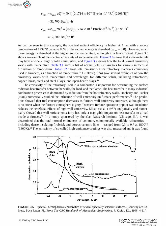
e T2 2 1
4 8 2 4 40 4 0 1714 10 2608µ µ−= = ( ) × °( ) °( )m m Btu hr ft R Rε σ . . - -
As can be seen in this example, the spectral radiant efficiency is higher at 3 µm with a source temperature of 1739°R because 80% of the radiant energy is absorbed (ε3 µm = 0.8). However, much more energy is absorbed at the higher source temperature, although it is less efficient. Figure 3.5 shows an example of the spectral emissivity of some materials. Figure 3.6 shows that some materials may have a wide a range of total emissivities; and Figure 3.7 shows how the total normal emissivity varies with temperature. Table 3.1 gives a list of normal total emissivities for various surfaces as a function of temperature. Table 3.2 shows total emissivities for refractory materials commonly used in furnaces, as a function of temperature.59 Glinkov (1974) gave several examples of how the emissivity varies with temperature and wavelength for different solids, including refractories, copper, brass, steel and steel alloys, and open-hearth slags.60
The emissivity of the refractory used in a combustor is important for determining the surface radiation heat transfer between the walls, the load, and the flame. The heat transfer in many industrial combustion processes is dominated by radiation from the hot refractory walls. Docherty and Tucker (1986) numerically studied the influence of wall emissivity on furnace performance.61 The predic-tions showed that fuel consumption decreases as furnace wall emissivity increases, although there is no effect when the furnace atmosphere is gray. Transient furnace operation or poor wall insulation reduces the beneficial effects of high wall emissivity. Elliston et al. (1987) analytically and numer-ically showed that wall surface emissivity has only a negligible impact on heat transfer to a load inside a furnace.62 In a study sponsored by the Gas Research Institute (Chicago, IL), it was determined that the total normal emittances of common, commercially available refractories — including dense insulating firebrick and porous ceramic fiber — ranged from 0.3 to 0.7 at 1800°F (1300K).63 The emissivity of so-called high-emittance coatings was also measured and it was found
FIGURE 3.5 Spectral, hemispherical emissivities of several spectrally selective surfaces. (Courtesy of CRC Press, Boca Raton, FL. From The CRC Handbook of Mechanical Engineering, F. Kreith, Ed., 1998, 4-61.)
e T
2
3 3 24 8 2 4 4
2
31 700
0 8 0 1714 10 1739
12 500
µ µ−
=
= = ( ) × °( ) °( )
=
m m
Btu hr ft
Btu hr ft R R
Btu hr ft
ε σ
,
. .
,
-
- -
-
© 2000 by CRC Press LLC

that few of the coatings actually had high emissivities. Those coatings could extend the range of refractory emittances from 0.3 to 0.9 at 1800°F (1300K). Another part of that study investigated the effect of using high-emittance coatings in large industrial furnaces.64 Testing was done on a 50-ton/hour (45 m-ton/hr) reheat furnace. Experimental results showed no significant change in furnace efficiency (at most, a 6% increase) using the highest available emissivity coatings on the refractory walls of the furnace. Another study showed that high-emissivity coatings applied to hundreds of furnaces in metallurgical, petrochemical, ceramic, mechanical, and other industries in the Peoples Republic of China showed energy savings of 5% to 10%, up to a maximum of 28%.65
The reported emissivity of the coating ranged from 0.80 to 0.92, depending on the surface temper-ature and wavelength.
FIGURE 3.6 Total emissivity ranges for various materials. (Courtesy of CRC Press, Boca Raton, FL.)
FIGURE 3.7 Total emissivity ranges vor various materials as a function of temperature. (Courtesy of CRC Press, Boca Raton, FL.)
© 2000 by CRC Press LLC

TABLE 3.1
Normal Total Emissivities of Various Surfaces as a Function of Temperature
Surface T (°C) Emissivity
A. Metals and their oxides Aluminum Polished 100 0.095 Commercial sheet 100 0.09 Heavily oxidized 95–505 0.20–0.31Brass Highly polished 73.2 Cu, 26.7 Zn 245–355 0.028–0.031 62.4 Cu, 36.8 Zn. 0.4 Pb, 0.3 Al 255–375 0.033–0.037 82.9 Cu, 17.0 Zn 275 0.030 Rolled plate, natural surface 20 0.06 Dull plate 50–350 0.22 Oxidized by heating at 600°C 200–600 0.61–0.59Copper Carefully polished electrolytic copper 80 0.018 Commercial emeried, polished, but pits remaining 20 0.030 Commercial, scraped shiny, but not mirrorlike 20 0.072 Plate, heated for a long time, covered with thick oxide layer 25 0.78 Molten copper 1075–1275 0.16–0.13Gold Pure, highly polished 225–625 0.018–0.035Iron and steel (not including stainless) Electrolytic iron, highly polished 175–225 0.052–0.064 Steel, polished 100 0.066 Iron, polished 425–1025 0.14–0.38 Cast iron, polished 200 0.21 Cast iron, newly turned 20 0.44 Cast iron, turned and heated 880–988 0.60–0.70 Mild steel, cleaned with organic solvents 25 0.12, 0.15Oxidized surfaces Iron plate, pickled, then rusted red 20 0.61 Iron plate, completely rusted 20 0.69 Rolled sheet steel 20 0.66 Cast iron, oxidized at 600°C 200–600 0.64–0.78 Steel, oxidized at 600°C 200–600 0.79Sheet steel With rough oxide layer 25 0.80 With shiny oxide layer 25 0.82 Steel plate, rough 40–370 0.94–0.97Molten surfaces Cast iron 1300–1400 0.29 Mild steel 1600–1800 0.28Lead Pure (99.6%) unoxidized 125–225 0.057–0.075 Oxidized at 150°C 200 0.63Mercury 0–100 0.09–0.12Nickel Electroplated, polished 25 0.045 Polished 100 0.072
© 2000 by CRC Press LLC

TABLE 3.1 (continued)
Electroplated, not polished 20 0.11 Plate, oxidized by heating at 600°C 200–600 0.37–0.48Nickel alloys Copper-nickel, polished 100 0.059 Nichrome wire, bright 50–1000 0.65–0.79Platinum Pure polished plate 225–625 0.054–0.104Silver Polished, pure 225–625 0.020–0.032Stainless steels Type 304 (8 Cr; 18 Ni) Polished 100 0.074 Light silvery, rough, brown, after heating 215–490 0.44–0.36 After 42 h at 525°C 215–525 0.62–0.73Thorium oxide 275–500 0.58–0.36Thorium oxide 500–825 0.36–0.21Tin Bright 50 0.06 Commercial tin-plated steel iron 100 0.07, 0.08Zinc Commercial 99.1% pure, polished 225–325 0.045–0.053 Oxidized by heating at 400°C 400 0.11 Galvanized sheet iron, fairly bright 30 0.23 Galvanized sheet iron, gray oxidized 25 0.28
B. Refractories, Building Materials, Paints, and Miscellaneous Materials Alumina (99.5–85 Al2O3; 0–12 SiO2; 0–1 Fe2O3) Effect of mean grain size 10 µm 1010–1565 0.30–0.18 50 µm 0.39–0.28 100 µm 0.50–0.40Alumina-silica (showing effect of Fe) 80–58 Al2O3; 16–38 SiO2; 0.4 Fe2O3 1010–1570 0.61–0.43 36–26 Al2O3; 50–60 SiO2; 1.7 Fe2O3 0.73–0.62 61 Al2O3; 35 SiO; 2.9 Fe2O3 0.78–0.68Asbestos Board 25 0.96 Paper 40–370 0.93–0.94Brick Red, rough, but no gross irregularities 20 0.93 Building 1000 0.45 Fireclay 1000 0.75Carbon Filament 1040–1405 0.526 Graphitized 100–320 0.76–0.75 Graphitized 320–500 0.75–0.71 Thin layer on iron plate 20 0.927 Thick coat 20 0.967
Normal Total Emissivities of Various Surfaces as a Function of Temperature
Surface T (°C) Emissivity
© 2000 by CRC Press LLC

TABLE 3.1 (continued)
In some industrial combustion processes, the surface absorptivity can change over time, which affects the performance of the system. This is particularly true in coal-fired processes where the ash may be deposited on tube surfaces. Wall et al. (1993) showed that the normal emittance of particulate ash is highly dependent on the particle size and surface temperature.66 In a subsequent study, Wall et al. (1995) studied the effects of ash deposits on the heat transfer in a coal-fired furnace.67 The heat transfer from the combustion products to the tubes is primarily by radiation, with a lesser amount by convection heating. The heat must conduct through the ash deposits and the tube wall, before heating the fluid inside the tubes primarily by convection. As the ash deposit melts to form a slag, the absorptance increases dramatically to values approaching 0.9. The thermal conductivity of the deposit is highly dependent on its physical state, especially its porosity. It is
Glass Smooth 20 0.94 Magnesite refractory brick 1000 0.38Paints, lacquers, varnishes Snow-white enamel varnish on rough iron plate Black shiny lacquer, sprayed on iron 25 0.875 Radiator paint; white, cream, bleach 100 0.79, 0.77, 0.84 Plaster, rough lime 10–90 0.91Quartz Rough, fused 20 0.93 Glass, 1.98 mm thick 280–840 0.90–0.41 Glass, 6.88 mm thick 280–840 0.93–0.47 Silica (98 SiO2; Fe-free), effect of grain size 10 µm 1010–1565 0.42–0.33 70–600 µm 0.62–0.46Water 0–100 0.95–0.963
Source: Courtesy of CRC Press, Boca Raton, FL.
TABLE 3.2Normal Total Emissivities of Refractories as a Function of Temperature
Temperature, °F (°C)
Material200(93)
400(200)
800(430)
1600(870)
2000(1090)
2400(1320)
2800(1540)
Fireclay brick 0.90 0.90 0.90 0.81 0.76 0.72 0.68Silica brick 0.90 — — 0.82–0.65 0.78–0.60 0.74–0.57 0.67–0.52Chrome-magnesite brick — — — 0.87 0.82 0.75 0.67Chrome brick 0.90 — — 0.97 0.98 — —High-alumina brick 0.90 0.85 0.79 0.50 0.44 — —Mullite brick — — — 0.53 0.53 0.62 0.63Silicon carbide brick — — — 0.92 0.89 0.87 0.86
Source: From D.H. Hubble, The Making, Shaping and Treating of Steel, 11th edition, Steelmaking and Refining Volume, R.J. Fruehan, Ed., AISE Steel Foundation, Pittsburgh, PA, 1998, 159-290.
Normal Total Emissivities of Various Surfaces as a Function of Temperature
Surface T (°C) Emissivity
© 2000 by CRC Press LLC
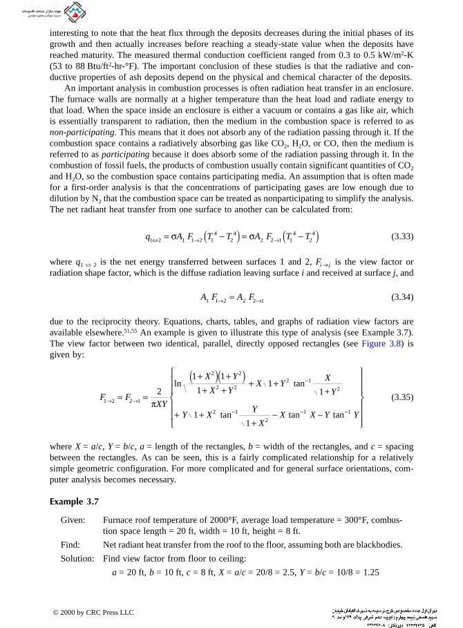
interesting to note that the heat flux through the deposits decreases during the initial phases of its growth and then actually increases before reaching a steady-state value when the deposits have
reached maturity. The measured thermal conduction coefficient ranged from 0.3 to 0.5 kW/m2-K (53 to 88 Btu/ft2-hr-°F). The important conclusion of these studies is that the radiative and con-ductive properties of ash deposits depend on the physical and chemical character of the deposits.
An important analysis in combustion processes is often radiation heat transfer in an enclosure. The furnace walls are normally at a higher temperature than the heat load and radiate energy to that load. When the space inside an enclosure is either a vacuum or contains a gas like air, which is essentially transparent to radiation, then the medium in the combustion space is referred to as non-participating. This means that it does not absorb any of the radiation passing through it. If the combustion space contains a radiatively absorbing gas like CO2, H2O, or CO, then the medium is referred to as participating because it does absorb some of the radiation passing through it. In the combustion of fossil fuels, the products of combustion usually contain significant quantities of CO2
and H2O, so the combustion space contains participating media. An assumption that is often made for a first-order analysis is that the concentrations of participating gases are low enough due to dilution by N2 that the combustion space can be treated as nonparticipating to simplify the analysis. The net radiant heat transfer from one surface to another can be calculated from:
(3.33)
where q1 ⇔ 2 is the net energy transferred between surfaces 1 and 2, Fi → j is the view factor or radiation shape factor, which is the diffuse radiation leaving surface i and received at surface j, and
(3.34)
due to the reciprocity theory. Equations, charts, tables, and graphs of radiation view factors are available elsewhere.51,55 An example is given to illustrate this type of analysis (see Example 3.7). The view factor between two identical, parallel, directly opposed rectangles (see Figure 3.8) is given by:
(3.35)
where X = a/c, Y = b/c, a = length of the rectangles, b = width of the rectangles, and c = spacing between the rectangles. As can be seen, this is a fairly complicated relationship for a relatively simple geometric configuration. For more complicated and for general surface orientations, com-puter analysis becomes necessary.
Example 3.7
Given: Furnace roof temperature of 2000°F, average load temperature = 300°F, combus-tion space length = 20 ft, width = 10 ft, height = 8 ft.
Find: Net radiant heat transfer from the roof to the floor, assuming both are blackbodies.
Solution: Find view factor from floor to ceiling:
a = 20 ft, b = 10 ft, c = 8 ft, X = a/c = 20/8 = 2.5, Y = b/c = 10/8 = 1.25
q A F T T A F T T1 2 1 1 2 14
24
2 2 1 14
24
⇔ → →= −( ) = −( )σ σ
A F A F1 1 2 2 2 1→ →=
F FXY
X Y
X YX Y
X
+Y
Y XY
XX X Y Y
1 2 2 1
2 2
2 22 1
2
2 1
2
1 1
2
1 1
11
1
11
→ →
−
− − −
= =π
+( ) +( )+ +
+ +
+ ++
− −
⎧
⎨
⎪⎪
⎩
⎪⎪
⎫
⎬
⎪⎪
⎭
⎪⎪
ln tan
tan tan tan
© 2000 by CRC Press LLC

Using the formula above for the view factor between parallel rectangles,
F1 → 2 = 0.356
T1 = 2000°F = 2460°R, T2 = 300°F = 760°R
q1 → 2 = (0.1714 × 10⁻⁸ Btu/hr-ft2-°R4)(0.356)(20 ft × 10 ft)[(2460°R)4 – (760°R)4]
= 4.43 × 10⁶ Btu/hr
Beér studied flame impingement inside a furnace and experimentally determined that radiation was at least 10% of the total heat flux.11 It was not specified how much of that radiation came from the hot walls and how much came from the flame. Vizioz27 and Smith29 studied flame impingement on a flat plate in a hot furnace. It was determined that radiation and convection were of comparable magnitude. Vizioz measured radiation to be 4% to 100% of the total heat flux. Smith calculated the surface radiant emission to the target, using Hottel’s zone method.51 It was 30% to 43% and 10% to 17% of the total heat transfer to water-cooled and air-cooled flat plates, respectively. Matsuo studied turbulent, preheated air/coke oven gas flames, impinging on a metal slab, inside a hot furnace.30 The top of the slab was exposed to the impinging flame. The rest was exposed to the radiation from the furnace walls. Furnace radiation was the dominant mechanism: (1) for large L, (2) for high tw , and (3) for large R. Ivernel calculated the radiation from hot furnace walls to a hemi-nosed cylinder.32 It was up to 42% of the total heat flux for impinging O2 /natural gas flames. You measured the convective and total heat flux, using gages plated with gold and black foils, respectively.23 By subtracting the convection from the total heat flux, radiation was calculated to be up to 35% of the convective flux. Van der Meer estimated that the radiation, from the hot inner refractory wall of a tunnel burner, was up to 15% of the total heat flux to the target.38
3.3.2 NONLUMINOUS GASEOUS RADIATION
3.3.2.1 Theory
The equation of radiative transfer will not be considered here as it is discussed in many radiation textbooks and is not commonly used as such to solve industrial combustion problems. The complete combustion of hydrocarbon fuels produces, among other things, CO2 and H2O. These gaseous products generate nonluminous radiation, which has been extensively studied.52 This heat transfer mode depends on the gas temperature level, the partial pressure and concentration of each species, and the molecular path length through the gas. Based on the study of CO flames, Garner (1965) concluded that most of the radiant energy from the flames was primarily chemiluminescence,68 but
FIGURE 3.8 Geometry for radiation between parallel plates.
© 2000 by CRC Press LLC

this was later proven to be wrong.69 Ludwig et al. (1973) gave a very detailed discussion of the theory of infrared radiation from combustion gases, including the terms and their definitions,
calculation techniques for both homogeneous and inhomogeneous gases, models for specific mol-ecules (both diatomic and polyatomic), actual computed radiation data, a discussion of the accuracy of the models, and some predictive techniques for calculating rocket exhausts.70 Examples of the spectral emissivity of H2O and CO2 as functions of wavelength and path length are shown in Figures 3.9 and 3.10, respectively.
FIGURE 3.9 Calculated spectral emissivity of H2O as a function of wavelength and path length. (From Handbook of Infrared Radiation from Combustion Gases, Ludwig et al., Eds., NASA, 1973, 241.)
© 2000 by CRC Press LLC
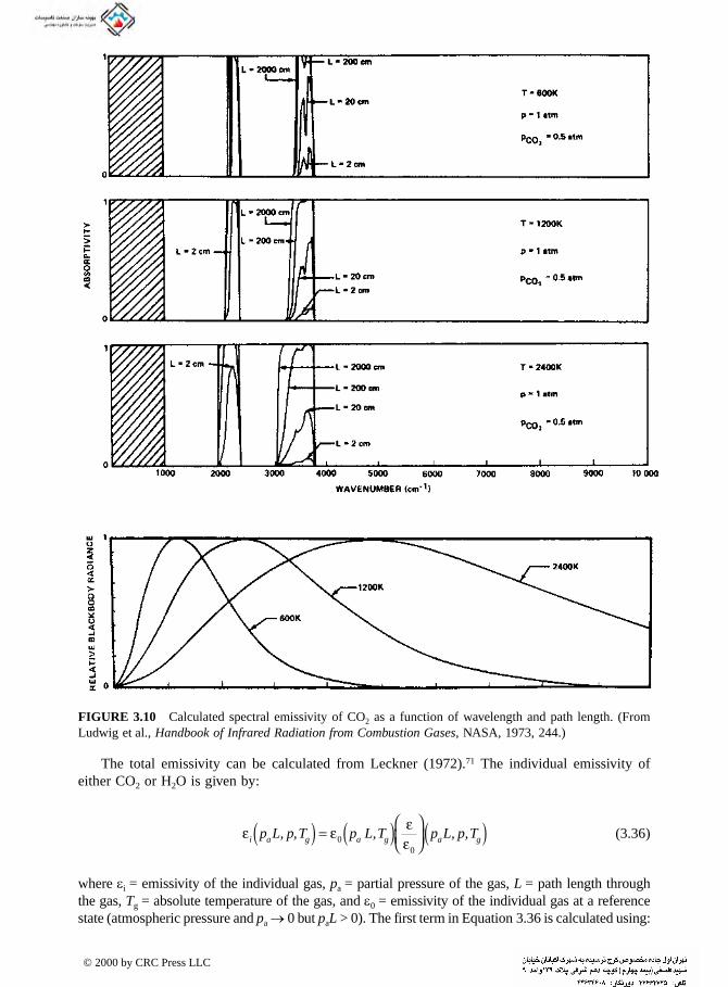
The total emissivity can be calculated from Leckner (1972).71 The individual emissivity of either CO2 or H2O is given by:
(3.36)
where εi = emissivity of the individual gas, pa = partial pressure of the gas, L = path length through the gas, Tg = absolute temperature of the gas, and ε0 = emissivity of the individual gas at a reference state (atmospheric pressure and pa → 0 but paL > 0). The first term in Equation 3.36 is calculated using:
FIGURE 3.10 Calculated spectral emissivity of CO2 as a function of wavelength and path length. (From Ludwig et al., Handbook of Infrared Radiation from Combustion Gases, NASA, 1973, 244.)
ε ε εεi a g a g a gp L p T p L,T p L, p,T, ,( ) = ( )⎛⎝⎜⎞⎠⎟( )0
0
© 2000 by CRC Press LLC

TABLE 3.3
(3.37)
where T0 = absolute reference temperature of the gas (1000K) and cij are constants. The second term in Equation 3.36 is calculated from:
(3.38)
where a, b, c, PE, and (paL)m/paL are given in Table 3.3. Graphical results for H2O and CO2 are shown in Figures 3.11 and 3.12, respectively. The total emissivity is then calculated using:
(3.39)
where the ∆ε accounts for the overlap between the H2O and CO2 bands and is calculated from:
(3.40)
and
(3.41)
Correlation Constants for Gas Emissivity Equations
Gas Water Vapor Carbon Dioxide
M, N 2,2 2,3–2.21180.85667
–0.10838
–1.19870.93048
–0.17156
0.035596–0.143910.045915
–3.98931.2710
–0.23678
2.7669–1.10900.19731
–2.10811.0195
–0.19544
0.39163–0.21897
0.044644
PE (p + 0.28pa)/p0
(paL)m/(paL)0 13.2t2 0.054/t2, t < 0.70.225t2, t > 0.7
a2.144, t < 0.75 1 + 0.1/t1.45
1.88 – 2.053 log10 t, t > 0.75b 1.10/t1.4 0.23c 0.5 1.47
Note: T0 = 1000 K, p0 = 1 bar, t = T/T0, (pa L)0 = 1 bar cm.
Source: From F. Kreith, Ed., CRC Handbook of Mechanical Engineering, CRC Press, Boca Raton, FL, 1998, 4-73.
c00
L cN 1
M O M
c0 M
L cNM
( p + 2.56 pa
/ t ) / p0
ε00
10
000
p L,T cT
T
p L
p La g ijg
j
a
a
i
j
N
i
M
( ) = ⎛⎝⎜⎞⎠⎟ ( )⎛
⎝⎜
⎞
⎠⎟
⎡
⎣
⎢⎢
⎤
⎦
⎥⎥
==∑∑exp log
εε0
10
2
11 1
1
⎛⎝⎜⎞⎠⎟( ) = −
−( ) −( )+ − +
−( )⎛
⎝⎜
⎞
⎠⎟
⎡
⎣
⎢⎢
⎤
⎦
⎥⎥
⎧⎨⎪
⎩⎪
⎫⎬⎪
⎭⎪p L, p,T
a P
a b Pc
p L
p La gE
E
a m
a
exp log
ε ε ε εCO H O CO H O2 2 2 2+ = + − ∆
∆ε ξξ
ξπ
=+
−⎛⎝⎜
⎞⎠⎟
+( )( )
⎛
⎝⎜⎜
⎞
⎠⎟⎟10 7 101
0 0089 10 410
0
2 76
2 2
.. log.
.
H O COp L
p La
ξ =+
p
p pH O
H O CO
2
2 2
© 2000 by CRC Press LLC

Example 3.8
Given: Combustion products containing 9% CO2, 18% H2O, and the balance N2, at a temperature of 1500°F, with a mean beam length of 10 ft, and at atmospheric pressure.
Find: Gas emissivity.
Solution: Calculate paL for CO2 and H2O to use graphs:
CO2: paL = (0.09 bar)(305 cm) = 27 bar-cm
H2O: paL = (0.18 bar)(305 cm) = 55 bar-cm
Look up on graphs the ε0 for CO2 and H2O at a temperature of 820°C:
CO2: ε0 Ý 0.12
H2O: ε0 Ý 0.29
Calculate correction factors ε/ε0 using Equation 3.38 and Table 3.3:
t = T/T0 (1090K/1000K) = 1.09
CO2: PE = (1.0 + 0.28(0.09))/1.0 = 1.03
H2O: PE = (1.0 + 2.56/ )/1.0 = 3.45
CO2:
FIGURE 3.11 Total emissivity of water vapor at the reference state of a total gas pressure p = 1 bar and a partial pressure of H2O pa → 0. (Courtesy of CRC Press, Boca Raton, FL. From The CRC Handbook of Mechanical Engineering, F. Kreith, Ed., 1998, 4-74.)
1.09
p L
p Lta m
a
( )= = ( ) =0 225 0 225 1 09 0 2672 2. . . .
© 2000 by CRC Press LLC

H2O:
CO2: a = 1 + 0.1/(1.09)1.45 = 1.09; b = 0.23; c = 1.47
H2O: a = 1.88 – 2.053 log10(1.09) = 1.80; b = 1.10/(1.09)1.4 = 0.97; c = 0.5
CO2: =
H2O: =
CO2: ε = (ε/ε0) ε0 = (1.001)(0.12) = 0.120
H2O: ε = (ε/ε0) ε0 = (1.184)(0.29) = 0.343
Calculate ξ:
Calculate ∆ε:
∆ε = 0.051
ε = 0.120 + 0.343 – 0.051 = 0.412
FIGURE 3.12 Total emissivity of carbon dioxide at the reference state of a total gas pressure p = 1 bar and a partial pressure of CO2 pa → 0. (Courtesy of CRC Press, Boca Raton, FL. From The CRC Handbook of Mechanical Engineering, F. Kreith, Ed., 1998, 4-75.)
p L
p Lta m
a
( )= = ( ) =13 2 13 2 1 09 15 72 2. . . .
εε0
10
21
1 09 1 1 1 031 09 0 23 1 1 03
1 47 0 267 1 001⎛⎝⎜⎞⎠⎟= − −( ) −( )
+ − +− ( )[ ]⎧
⎨⎩
⎫⎬⎭=. .
. . .exp . log . .
εε0
10
21
1 80 1 1 3 451 80 0 07 1 3 45
0 5 15 7 1 184⎛⎝⎜⎞⎠⎟= − −( ) −( )
+ − +− ( )[ ]⎧
⎨⎩
⎫⎬⎭=. .
. . .exp . log . .
ξ =+
=0 180 18 0 09
0 67.
. ..
∆ε =+ ( ) − ( )⎛
⎝⎜⎞⎠⎟
+( )( )⎛⎝⎜
⎞⎠⎟
0 6710 7 101 0 67
0 0089 0 670 18 0 09 305
110 4
10
.. .
. . log. .. cm
bar-cm
© 2000 by CRC Press LLC

The absorptivity of H2O and CO2 can be estimated using:
(3.42)
where Ts is the surface temperature such as a furnace wall. The correction for the band overlap between H2O and CO2 is calculated using:
(3.43)
where ∆ε is estimated with a pressure path length of paLTs /Tg .
Example 3.9
Given: Using the data from the previous example and a wall temperature of 1000°F.
Find: Gas absorptivity.
Solution: Calculate paLTs/Tg for CO2 and H2O to use graphs:
CO2: paLTs/Tg = (0.09 bar)(305 cm)(1000 + 460)/(1500 + 460) = 20 bar-cm
H2O: paLTs/Tg = (0.18 bar)(305 cm)(1000 + 460)/(1500 + 460) = 41 bar-cm
Look up on graphs the ε0 for CO2 and H2O at a temperature of 540°C (1000°F):
CO2: ε0 Ý 0.12, H2O: ε0 Ý 0.28
Calculate correction factors ε/ε0 using Equation 3.38 and Table 3.3:
t = (811K/1000K) = 0.811
CO2: PE = (1.0 + 0.28(0.09))/1.0 = 1.03
H2O: PE = (1.0 + 2.56/ )/1.0 = 3.84
CO2:
H2O:
CO2: a = 1 + 0.1/(0.811)1.45 = 1.14; b = 0.23; c = 1.47
H2O: a = 1.88 – 2.053 log10(0.811) = 2.07; b = 1.10/(0.811)1.4 = 1.47; c = 0.5
CO2:
H2O:
CO2: ε = (ε/ε0) ε0 = (1.001)(0.12) = 0.120
H2O: ε = (ε/ε0) ε0 = (1.307)(0.28) = 0.366
CO2:
α εp L, p,T TT
Tp L
T
Tp,Ta g s
g
sa
s
gs, ,( ) = ⎛
⎝⎜⎞⎠⎟⎛
⎝⎜
⎞
⎠⎟
1 2
α α α εCO H O CO H O2 2 2 2+ = + − ∆
0.811
p L
p Lta m
a
( )= = ( ) =0 225 0 225 0 811 0 1482 2. . . .
p L
p Lta m
a
( )= = ( ) =13 2 13 2 0 811 8 682 2. . . .
εε0
10
21
1 14 1 1 1 031 14 0 23 1 1 03
1 47 0 148 1 001⎛⎝⎜⎞⎠⎟= − −( ) −( )
+ − +− ( )[ ]⎧
⎨⎩
⎫⎬⎭=. .
. . .exp . log . .
εε0
10
21
2 07 1 1 3 842 07 1 47 1 3 84
0 5 8 68 1 307⎛⎝⎜⎞⎠⎟= − −( ) −( )
+ − +− ( )[ ]⎧
⎨⎩
⎫⎬⎭=. .
. . .exp . log . .
α = ++
( ) =1500 4601000 460
0 120 0 139. .
© 2000 by CRC Press LLC

H2O: α = +
+=1500 460
1000 4600 366 0 424. .
α = 0.139 + 0.424 – 0.051 = 0.512
Relatively simple but accurate calculations for isothermal gases, which are absorbing-emitting but not scattering, in an isothermal black-walled enclosure can be computed using:
(3.44)
where Lm is the average mean beam length and Tw is the absolute temperature of the isothermal wall. The mean beam length is a function of the geometry of the enclosure and can be calculated using the formulas in Table 3.4. For geometries not listed in that table, the following formula can be used:
Lm = 3.6 V/A (3.45)
where V is the volume of the enclosure and A is the surface area inside the enclosure. Gulic (1974) gave a modified form to calculate the mean beam length:72
(3.46)
where τ is the optical density of the gas.Cess (1974) has given a relatively simple procedure for calculating infrared gaseous radiation
that uses an analytical approximate band model.73 The results showed good agreement with a numerical solution. Greif (1974) presented some experimental and theoretical results for infrared radiation from a turbulent flow of air, CO2, and steam.74 Kovotny (1974) showed the importance of pressure in calculating gaseous radiation heat transfer.75 In a review paper, Edwards (1976) cautioned about the use of gray-gas models and analysis to represent the truly spectrally-dependent phenomena of gaseous radiation.76 Trout (1977) gave some simple methods for estimating both nonluminous and luminous radiation from industrial flames.77 Tien and co-workers (1968, 1982) reviewed radiation from flames.78,79 They extensively reviewed the available models for both nonluminous and luminous gaseous radiation. Edwards and Balakrishnan (1973) presented some correlations for calculating the radiative properties of H2O, CO2, CO, NO, SO2, and CH4 for use in solving gas radiation problems.80 Taylor and Foster (1974) presented empirical curve-fitted equations for the total emissivities of nonluminous and luminous flames for CO2 –H2O and CO2 –H2O–soot mixtures arising in oil and gas combustion.81 Coppalle and Vervisch (1983) calcu-lated the total emissivities of high-temperature (2000–3000K) gases (CO2 –H2O mixtures).82
Edwards and Matavosian (1984) developed some scaling rules for calculating the total absorptivity and emissivity of gases and tabulated and graphed results for various combinations of gas compo-sition, product of partial pressure times the path length, and gas temperature.83 Howell (1988) reviewed thermal radiation in participating media and gave numerous references for further infor-mation.84 The P-N, two-flux, discrete ordinate, finite element, zoning, and Monte Carlo methods of analysis were briefly discussed. Wieringa et al. (1990) modeled the spectral radiation produced by natural gas flames in a regenerative glass furnace.85 The spectral radiation from H2O and CO2
were modeled using 15 spectral bands. The numerical results showed that the furnace wall emis-sivity had only minimal impact on the furnace efficiency.
q L T L Tm w m g= − ( )[ ] − ( ) σ α ε1 4 4
LVA
ee em = − + +
⎛⎝⎜
⎞⎠⎟
−
− −3 61
.τ
τ τ
τ
τ τ
© 2000 by CRC Press LLC

TABLE 3.4
3.3.2.2 Combustion Studies
Two types of nonluminous radiation measurements have been made in previous combustion studies: total and spectral. The total radiation measurements were typically made with some type of detector that measured the overall radiation received, with no wavelength dependence. More recent mea-surements have been made that gave the radiation as a function of wavelength. These two methods of measurements applied to nonluminous radiation are discussed briefly here.
3.3.2.2.1 Total radiationIn some previous combustion experimental studies, nonluminous gaseous radiation has been sig-nificant. Kilham tested nearly stoichiometric, laminar air/CO flames, impinging normal to an uncooled refractory cylinder.14 Flame radiation was 5% to 16% of the total heat flux. Jackson also tested laminar flames, impinging normal to refractory cylinders. A variety of fuels, oxidizers, and stoichiometries were tested. The measured flame radiation was up to 5% of the total heat flux. Dunham tested nearly stoichiometric, laminar air/CO flames, impinging normal to the nose of a hemi-nosed cylinder.86 The estimated nonluminous radiation was up to 13% of the total heat flux.
Mean Beam Lengths for Radiation Calculations
Geometry of Gas Volume
Characterizing Dimension
L
Geometric MeanBeam Length
L0/L
Average MeanBeam Length
Lm/L Lm/L0
Sphere radiating to its surface Diameter, L = D 0.67 0.65 0.97Infinite circular cylinder to bounding
surfaceDiameter, L = D 1.00 0.94 0.94
Semi-infinite circular cylinder to: Diameter, L = D Element at center of base 1.00 0.90 0.90 Entire base 0.81 0.65 0.80Circular cylinder
(height/diameter = 1) to:Diameter, L = D
Element at center of base 0.76 0.71 0.92 Entire surface 0.67 0.60 0.90Circular cylinder
(height/diameter = 2) to:Diameter, L = D
Plane base 0.73 0.60 0.82 Concave surface 0.82 0.76 0.93 Entire surface 0.80 0.73 0.91Circular cylinder
(height/diameter = 0.5) to:Diameter, L = D
Plane base 0.48 0.43 0.90 Concave surface 0.53 0.46 0.88 Entire surface 0.50 0.45 0.90Infinite semicircular cylinder to center
of plane rectangular faceRadius, L = R — 1.26 —
Infinite slab to its surface Slab thickness, L 2.00 1.76 0.88Cube to a face Edge L 0.67 0.6 0.90Rectangular 1 × 1 × 4 parallelepipeds: Shortest edge, L To 1 × 4 face 0.90 0.82 0.91 To 1 × 1 face 0.86 0.71 0.83 To all faces 0.89 0.81 0.91
Source: From CRC Handbook of Chemistry and Physics, 79th edition, CRC Press, Boca Raton, FL, 1998, 12-191–12-192.
© 2000 by CRC Press LLC
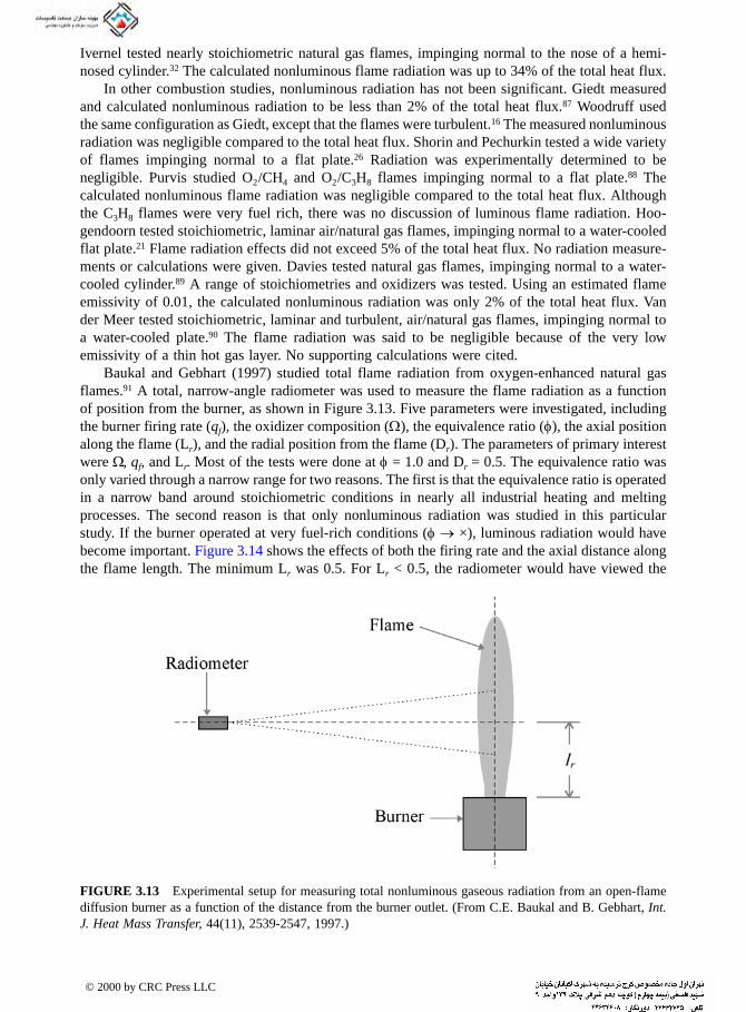
Ivernel tested nearly stoichiometric natural gas flames, impinging normal to the nose of a hemi-nosed cylinder.32 The calculated nonluminous flame radiation was up to 34% of the total heat flux.
In other combustion studies, nonluminous radiation has not been significant. Giedt measured
and calculated nonluminous radiation to be less than 2% of the total heat flux.87 Woodruff used the same configuration as Giedt, except that the flames were turbulent.16 The measured nonluminous radiation was negligible compared to the total heat flux. Shorin and Pechurkin tested a wide variety of flames impinging normal to a flat plate.26 Radiation was experimentally determined to be negligible. Purvis studied O2 /CH4 and O2 /C3H8 flames impinging normal to a flat plate.88 The calculated nonluminous flame radiation was negligible compared to the total heat flux. Although the C3H8 flames were very fuel rich, there was no discussion of luminous flame radiation. Hoo-gendoorn tested stoichiometric, laminar air/natural gas flames, impinging normal to a water-cooled flat plate.21 Flame radiation effects did not exceed 5% of the total heat flux. No radiation measure-ments or calculations were given. Davies tested natural gas flames, impinging normal to a water-cooled cylinder.89 A range of stoichiometries and oxidizers was tested. Using an estimated flame emissivity of 0.01, the calculated nonluminous radiation was only 2% of the total heat flux. Van der Meer tested stoichiometric, laminar and turbulent, air/natural gas flames, impinging normal to a water-cooled plate.90 The flame radiation was said to be negligible because of the very low emissivity of a thin hot gas layer. No supporting calculations were cited.
Baukal and Gebhart (1997) studied total flame radiation from oxygen-enhanced natural gas flames.91 A total, narrow-angle radiometer was used to measure the flame radiation as a function of position from the burner, as shown in Figure 3.13. Five parameters were investigated, including the burner firing rate (qf), the oxidizer composition (Ω), the equivalence ratio (φ), the axial position along the flame (Lr), and the radial position from the flame (Dr). The parameters of primary interest were Ω, qf, and Lr. Most of the tests were done at φ = 1.0 and Dr = 0.5. The equivalence ratio was only varied through a narrow range for two reasons. The first is that the equivalence ratio is operated in a narrow band around stoichiometric conditions in nearly all industrial heating and melting processes. The second reason is that only nonluminous radiation was studied in this particular study. If the burner operated at very fuel-rich conditions (φ → ×), luminous radiation would have become important. Figure 3.14 shows the effects of both the firing rate and the axial distance along the flame length. The minimum Lr was 0.5. For Lr < 0.5, the radiometer would have viewed the
FIGURE 3.13 Experimental setup for measuring total nonluminous gaseous radiation from an open-flame diffusion burner as a function of the distance from the burner outlet. (From C.E. Baukal and B. Gebhart, Int. J. Heat Mass Transfer, 44(11), 2539-2547, 1997.)
© 2000 by CRC Press LLC

flame and part of the burner itself. At low firing rates, the flame radiation decreased rapidly with the distance from the burner exit. At intermediate and higher firing rates, the flame radiation was relatively constant for Lr from about 2 to 5. Figure 3.15 is a similar graph except that the oxidizer composition, instead of the firing rate, was varied. The flame radiation was relatively constant over a wide range of Lr, for Ω = 1.0. At Ω = 0.35, the peak flame radiation occurred at about Lr = 1.5 and then slowly decreased with Lr. Figure 3.16 shows how the radial location of the radiometer affected the measurements. At Dr = 1.0, the radiometer viewed the entire width of the flame. The effective path length decreased as Dr increased because the flame had a circular cross-section. This reduced the average flame radiation as shown in the plot. However, the reduction was relatively small. Figure 3.17 shows how the equivalence ratio and the oxidizer compositions affected the flame radiation. For the smaller Ω, the highest flame radiation occurred at slightly fuel-lean conditions. For a pure O2 oxidizer, the highest flame radiation occurred in a band around stoichi-ometric conditions (φ = 1.0). Figure 3.18 shows how the flame radiation varied as a function of the oxidizer composition for a fixed firing rate and equivalence ratio. The only parameter that was varied was the amount of N2 in the oxidizer. The fuel and O2 flow rates were constant. Ren decreased from 6800 to 2400 as Ω increased from 0.28 to 1.00. The plot shows that the flame radiation increased by more than 2.5 times by removing N2 from the oxidizer. This is a result of higher flame temperatures and partial pressures of CO2 and H2O. Figure 3.19 shows how the flame radiationincreased as the firing rate increased and as the equivalence ratio increased. Figure 3.20 is a plot of flame radiation as a function of the equivalence ratio and the firing rate for a constant Reynolds number of 4500. As N2 was removed from the oxidizer (Ω increasing), the firing rate had to be increased to maintain a fixed Ren. This shows that a higher heat release density may be achieved by increasing the O2 concentration in the oxidizer, for a given nozzle diameter. It also implies that Ren by itself is not a sufficient parameter to indicate the performance of oxygen-enhanced flames. The oxidizer composition Ω must also be specified. Figure 3.21 shows the peak flame radiation measured for a given firing rate and oxidizer composition. For Ω = 1.00, the peak radiation increased
FIGURE 3.14 Total nonluminous gaseous radiation (q″rad) as a function of distance from the burner (Lr) and firing rate (qf = 5.0, 15.0, 25.0 kW) for Ω = 1.00, φ = 1.00, Dr = 0.5. (From C.E. Baukal and B. Gebhart, Int. J. Heat Mass Transfer, 44(11), 2539-2547, 1997.)
© 2000 by CRC Press LLC
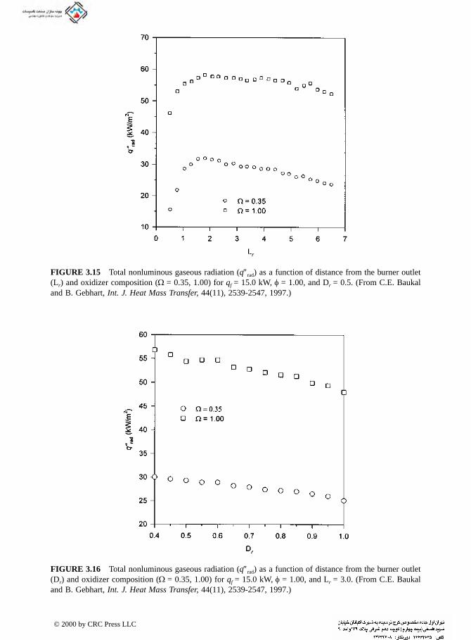
FIGURE 3.15 Total nonluminous gaseous radiation (q″rad) as a function of distance from the burner outlet (Lr) and oxidizer composition (Ω = 0.35, 1.00) for qf = 15.0 kW, φ = 1.00, and Dr = 0.5. (From C.E. Baukal and B. Gebhart, Int. J. Heat Mass Transfer, 44(11), 2539-2547, 1997.)
FIGURE 3.16 Total nonluminous gaseous radiation (q″rad) as a function of distance from the burner outlet (Dr) and oxidizer composition (Ω = 0.35, 1.00) for qf = 15.0 kW, φ = 1.00, and Lr = 3.0. (From C.E. Baukal and B. Gebhart, Int. J. Heat Mass Transfer, 44(11), 2539-2547, 1997.)
© 2000 by CRC Press LLC

FIGURE 3.17 Total nonluminous gaseous radiation (q″rad) as a function of the equivalence ratio (φ) and oxidizer composition (Ω = 0.35, 1.00) for qf = 15.0 kW, Lr = 3.0, and Dr = 0.5. (From C.E. Baukal and B. Gebhart, Int. J. Heat Mass Transfer, 44(11), 2539-2547, 1997.)
FIGURE 3.18 Total nonluminous gaseous radiation (q″rad) as a function of the oxidizer composition (Ω)for qf = 15.0 kW, φ = 1.00, Lr = 3.0, and Dr = 0.5. (From C.E. Baukal and B. Gebhart, Int. J. Heat Mass Transfer, 44(11), 2539-2547, 1997.)
© 2000 by CRC Press LLC
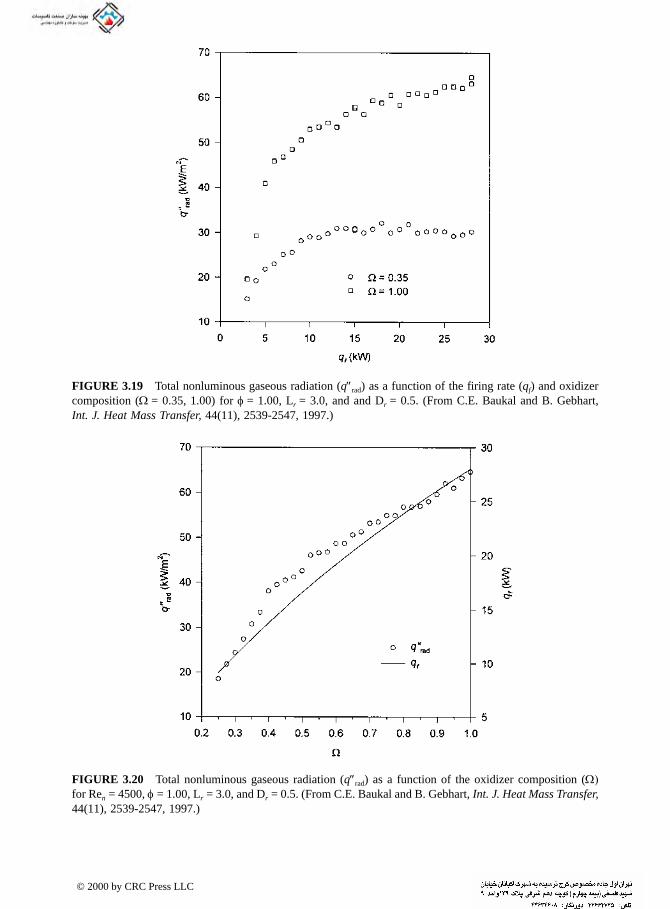
FIGURE 3.19 Total nonluminous gaseous radiation (q″rad) as a function of the firing rate (qf) and oxidizer composition (Ω = 0.35, 1.00) for φ = 1.00, Lr = 3.0, and and Dr = 0.5. (From C.E. Baukal and B. Gebhart, Int. J. Heat Mass Transfer, 44(11), 2539-2547, 1997.)
FIGURE 3.20 Total nonluminous gaseous radiation (q″rad) as a function of the oxidizer composition (Ω)for Ren = 4500, φ = 1.00, Lr = 3.0, and Dr = 0.5. (From C.E. Baukal and B. Gebhart, Int. J. Heat Mass Transfer,44(11), 2539-2547, 1997.)
© 2000 by CRC Press LLC

with the firing rate. For Ω = 0.35, the peak radiation was relatively constant over a wide range of firing rates. Figure 3.22 shows the approximate axial location for the peak flame radiation. Initially, the peak flame locations were closer to the burner for Ω = 1.00, compared to Ω = 0.35. At higher firing rates, this trend reversed. For Ω = 1.00, these locations were fairly well-defined. For Ω = 0.35, there was a range of positions along the flame length where the maximum flame radiation values were obtained. The locations given in the figure are approximately in the center of the range. Figure 3.23 is a plot of the location for the peak flame radiation that has been normalized to the visible length of the flame. This shows that for high Ω flames, the axial location of the peak flame radiation was at about 14% of the visible flame length. For the lower Ω flames, this location was between about 9% and 15% of the flame length.
The important conclusions of the study were:
1. Thermal radiation increased dramatically by removing N2 from the oxidizer2. The flame radiation increased with the firing rate with a more dramatic increase at higher
O2 concentrations in the oxidizer3. Higher flame radiation was measured at or near stoichiometric conditions where typical
industrial heating processes are operated4. For higher firing rates, the radiation was nearly constant over a wide range of axial
locations in the flame5. At lower firing rates, the flame radiation decreased with the axial distance from the
burner outlet
For higher O2 concentrations, the peak flame radiation increased with the firing rate. For lower O2
concentrations, the peak flame radiation was nearly constant over a wide range of firing rates. The location of the peak flame radiation varied from 9% to 15% of the visible flame length. This location was more defined for the higher O2 flames in terms of both its absolute position and of the position normalized by the flame length.
FIGURE 3.21 Maximum total nonluminous gaseous radiation (q″rad) as a function of the firing rate (qf) and oxidizer composition (Ω = 0.35, 1.00) for φ = 1.00 and Dr = 0.5 with Lr variable. (From C.E. Baukal and B. Gebhart, Int. J. Heat Mass Transfer, 44(11), 2539-2547, 1997.)
© 2000 by CRC Press LLC
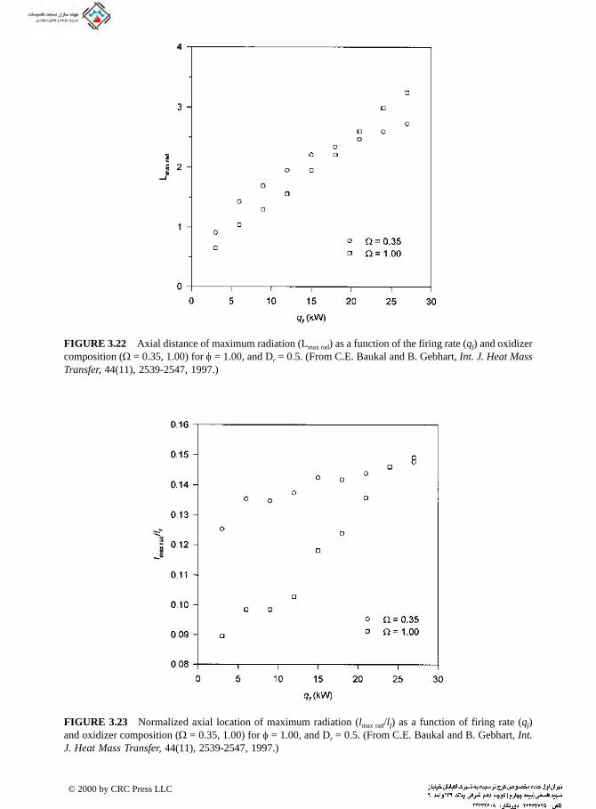
FIGURE 3.22 Axial distance of maximum radiation (Lmax rad) as a function of the firing rate (qf) and oxidizer composition (Ω = 0.35, 1.00) for φ = 1.00, and Dr = 0.5. (From C.E. Baukal and B. Gebhart, Int. J. Heat Mass Transfer, 44(11), 2539-2547, 1997.)
FIGURE 3.23 Normalized axial location of maximum radiation (lmax rad/lf) as a function of firing rate (qf) and oxidizer composition (Ω = 0.35, 1.00) for φ = 1.00, and Dr = 0.5. (From C.E. Baukal and B. Gebhart, Int. J. Heat Mass Transfer, 44(11), 2539-2547, 1997.)
© 2000 by CRC Press LLC

3.3.2.2.2 Spectral radiationJi and Baukal (1998) did the first systematic experimental study of the nonluminous and luminous spectral radiation from oxygen-enhanced flames.92 Two common quantities are measured in spectral radiometry: spectral radiance and spectral irradiance. Spectral radiance quantifies the energy flux in a unit wavelength interval that is emitting from a source surface per unit area and unit solid angle. The spectral irradiance is a measure of the energy flux in a unit wavelength interval that is incident onto a target surface per unit area. For an optical source with a well-defined uniform emitting surface, spectral radiance can be measured accurately and converted into spectral irradi-ance. The lack of such well-defined and uniform radiating surfaces for flames renders the mea-surement of spectral radiance impractical. However, spectral irradiance is still a valid quantity to measure in flames and has more practical meaning in heat transfer to targets. For this reason, spectral irradiance was measured, despite the fact that spectral radiance has been used in some previous theoretical studies on flame radiation.44
A custom-built version of the commercial ICSM burner from Nordsea Gas Technology Ltd. (Cheshire, England) was used for the study, as shown in Figure 3.24, where dn = 38.5 mm. It was a round form of the rectangular burners93 used in industrial heating and melting processes. Details of this burner and its operating characteristics, as well as fuel and oxidizer flow specifications, are given elsewhere.94 A key feature of the burner was the wide variety of oxidizers that could be used, ranging from air to pure oxygen, for a range of firing rates. Another key feature was that the burner produced a uniform, nearly one-dimensional flame, so that the flame radiation was more uniform compared to diffusion flames. A firing rate of 17,000 Btu/hr (5.0 kW) was used for most of the measurements, so that there was no significant radiation at a height 1.6 ft (0.5 m) above the burner surface.
As shown in Figure 3.25, three spectral monochromators were set at 11 ft (3.5 m) away from the burner centerline, and 0.82 ft (0.25 m) above the burner surface so that their field of view covered the entire radiation length of the flames. Because the flames were in open air, without any furnace enclosure and without impinging on any targets or nearby walls, ambient emission and reflection from the surroundings were negligible. Three parameters were varied to study their effects on the spectral radiation from oxygen-enhanced/natural gas flames: oxygen enrichment ratio (Ω),fuel equivalence ratio (φ), and firing rate or fuel input (qf). The oxygen enrichment ratio ranged from Ω = 0.21 (air) to Ω = 1.00 (pure O2). For the specific natural gas composition used, the stoichiometric ratio of oxygen:fuel was 2.08. Fuel-rich and fuel-lean flames had fuel equivalence ratios >1.0 and <1.0, respectively.
FIGURE 3.24 Burner used for flame radiation study using oxygen-enhanced burners. (From C.E. Baukal, Heat Transfer from Flames Impinging Normal to a Plane Surface, Ph.D. thesis, University of Pennsylvania, 1996.)
© 2000 by CRC Press LLC

As will be shown in the flame radiation spectra, most of the flame radiation fell within the infrared region. Ultraviolet (0.25–0.38 µm) radiation, while important in some flame diagnostics, contributed little to the total radiation intensity. Visible (0.38–0.78 µm) radiation also made only a small contribution to the total radiation intensity. However, as shown later (Chapter 4), the visible radiation is a direct indicator of the penetrating radiation that is most effective for glass heating and melting. For a relative comparison among the flames studied, the radiation spectra over the entire wavelength region (0.25–5.0 µm) was numerically integrated and then normalized to the integrated radiation intensity of the flame with qf = 5.0 kW, Ω = 1.0, and φ = 1.0. This normalization eliminated possible errors due to the uncertainties in the spectral radiometer calibration. Normal-ization also helped to reveal the general trends as the flame parameters changed. The results are summarized in Figure 3.26, which shows three flame radiation spectra with qf = 5.0 kW, φ = 1.0,
FIGURE 3.25 Experimental setup of the Monolight spectral radiometer (UV-VIS = UV and visible, NIR = near-IR, and MIR = mid-IR). (From B. Ji and C.E. Baukal, Proc. 1998 Int. Gas Research Conf., Nov. 8-11, 1998, San Diego, CA, D. Dolenc, Ed., 5, 422-433, 1998.)
FIGURE 3.26 Overall spectra for flame radiation dependence on oxygen enrichment ratio Ω. (From B. Ji and C.E. Baukal, Proc. 1998 Int. Gas Research Conf., Nov. 8-11, 1998, San Diego, CA, D. Dolenc, Ed., 5, 422-433, 1998.)
© 2000 by CRC Press LLC

TABLE 3.5
and Ω = 1.00, 0.60, and 0.21, respectively. The integrated results are listed in Table 3.5. The radiation intensity from the pure oxygen/natural gas flame (Ω = 1.00) was about 4 times that from the air/natural gas flame (Ω = 0.21) for the same fuel consumption. This is because nitrogen in the air absorbs energy from the combustion reaction, but N2 does not radiate. Figure 3.27 is the UV portion of the spectra plotted on a logarithmic scale. Despite the relatively small contribution of UV radiation to the total intensity, the presence of UV emissions (predominantly from the elec-tronically excited OH radicals) can be explored as a way to visualize nonluminous flames in hot and highly luminous furnaces. The UV radiation from the pure oxygen flame was about 3 orders of magnitude stronger than that from the air/fuel flame. Such a dramatic difference cannot be simply accounted for by thermodynamic equilibrium at different flame temperatures. Rather, this was an indication that significantly more nonequilibrium chemiluminescence of OH radicals exists in oxygen-enhanced flames. It can be inferred that the OH emission-based band-reversal method, while successfully performed in CH4 /N2O flames,95 will not yield the correct flame temperature in oxygen-enhanced flames. Figure 3.28 shows three flame radiation spectra with qf = 5.0 kW, Ω = 1.0, and φ = 0.67, 1.00, and 2.00, respectively. The normalized total radiation intensities for φ in the range of 0.67 to 2.00 are summarized in Table 3.5. The reduced radiation intensities in the fuel lean cases (φ < 1.0) are due to the fact that excessive oxygen carries away heat, but does not radiate. Although the radiation intensities in the fuel-rich cases (φ > 1.0) are apparently less than that in the stoichiometric case (φ = 1.00), it should be noted that not all of the fuel was consumed due to lack of available oxygen. In a more realistic combustion system, oxygen would be introduced in a later stage to complete the combustion. With this in mind, the fuel-rich cases would actually provide more radiation for the same fuel consumption. Since the flames were in open air, actual equivalence ratios were different from the control settings, due to air entrainment. Nevertheless, the general trends remain the same.
The integrated spectral radiation intensities were nearly the same for stoichiometric flames with Ω = 1.00, qf = 5 kW and Ω = 0.60, qf = 7 kW. For a given O2 enrichment level, the radiation intensity increased more slowly than the increase in firing rate. Figure 3.29 shows radiation spectra from stoichiometric flames with different oxygen enrichment ratios and firing rates. The radiation intensity did not increase for air-fired flames (Ω = 0.21) when the firing rate increased from 5 kW
Flame Radiation Intensity Measurements
W φ Inrm(total) Inrm(pen.) Inrm(BK7) γ
1.00 0.67 0.90 ± 0.06 0.89 ± 0.06 0.82 ± 0.06 0.15 ± 0.011.00 0.80 0.99 ± 0.07 0.98 ± 0.07 0.95 ± 0.07 0.13 ± 0.011.00 1.00 1.00* 1.00* 1.00* 0.14 ± 0.011.00 1.33 0.93 ± 0.07 0.98 ± 0.07 0.99 ± 0.07 0.17 ± 0.011.00 1.50 0.91 ± 0.06 0.93 ± 0.07 0.87 ± 0.06 0.20 ± 0.011.00 1.60 0.84 ± 0.06 0.83 ± 0.06 0.88 ± 0.06 0.21 ± 0.011.00 1.79 0.80 ± 0.06 0.83 ± 0.06 0.83 ± 0.06 0.37 ± 0.031.00 1.89 0.75 ± 0.05 0.87 ± 0.06 0.96 ± 0.07 0.55 ± 0.041.00 2.00 0.80 ± 0.06 1.12 ± 0.08 1.10 ± 0.08 1.02 ± 0.070.60 1.00 0.73 ± 0.05 0.70 ± 0.05 0.75 ± 0.05 0.12 ± 0.010.21 1.00 0.26 ± 0.02 0.19 ± 0.01 0.19 ± 0.01 0.005 ± 0.001
* The Ω = 1.0 and φ = 1.0 intensities were used as the reference in the normalization.
Source: From B. Ji and C.E. Baukal, Proc. 1998 Int. Gas Research Conf.,
Nov. 8–11, 1998, San Diego, CA, D. Dolenc, Ed., 5, 422-433, 1998.
© 2000 by CRC Press LLC

to 10 kW. These trends for the change in radiation as a function of the firing rate are consistent with the findings in another study.94 While a quantitative comparison may depend on the specific
FIGURE 3.27 UV region of the spectra on a logarithmic scale for the flame radiation dependence on oxygen enrichment ratio Ω. (From B. Ji and C.E. Baukal, Proc. 1998 Int. Gas Research Conf., Nov. 8-11, 1998, San Diego, CA, D. Dolenc, Ed., 5, 422-433, 1998.)
FIGURE 3.28 Flame radiation dependence on fuel equivalence ratio φ. Spectra were plotted with qf = 5.0 kW, Ω = 1.0, and φ = 0.67, 1.00, and 2.00, respectively. (From B. Ji and C.E. Baukal, Proc. 1998 Int. Gas Research Conf., Nov. 8-11, 1998, San Diego, CA, D. Dolenc, Ed., 5, 422-433, 1998.)
© 2000 by CRC Press LLC

burner design, the qualitative trend is generally true. Nitrogen in the air reduces radiation intensity. Since increasing the firing rate in air/natural gas flames is accompanied by increasing nitrogen flow, the increase in combustion heat cannot be as efficiently released by radiation as in the oxygen-enriched flames.
3.3.3 LUMINOUS RADIATION
3.3.3.1 Theory
Luminous flames are produced by the continuous radiant emission of particles in the flame, such as soot, which radiate approximately as blackbodies. Yagi and Iino (1961) studied both the luminous (qrs = radiation from soot) and nonluminous (qrg = gaseous radiation) from turbulent diffusion flames.96 The comparison of the two types of radiation is shown in Figure 3.30, which shows that the soot radiation is greater than the gaseous radiation. Echigo et al. (1967) studied luminous radiation from flames.97 They noted that a rigorous definition of luminous and nonluminous flames does not exit. It had long been assumed that soot remains in the solid phase during the combustion process and emits a continuous spectrum of visible and infrared radiation. Based on experiments, they hypothesized that the dehydrogenation and polymerization of hydrocarbon fuels occurs in the liquid phase, and that the decomposed and polymerized compound (“pre-soot substance”) emits banded spectra; then, the soot particles agglomerate after dehydrogenation and polymerization are completed. Gray et al. (1976) noted three size categories for particles: large, small, and intermedi-ate.98 Particles absorb, diffract, or attenuate radiation to varying degrees depending on their size. The soot generated in a flame is highly dependent, among other things, on the fuel composition. Luminous radiation is usually important when liquid and solid fuels, like oil and coal, are used. It is usually not significant for gaseous fuels, like natural gas. Fuels with higher carbon-to-hydrogen weight ratios (see Table 3.6) tend to produce sootier flames. In a survey paper, Wagner (1978) reviewed soot formation in combustion.99 It was noted that soot forms at temperatures ranging from 1000 to 2500°C (1800 to 4500°F). Soot consists primarily of carbon, formed into long chains. The
FIGURE 3.29 Flame radiation dependence on firing rate and oxygen enrichment ratio. (From B. Ji and C.E. Baukal, Proc. 1998 Int. Gas Research Conf., Nov. 8-11, 1998, San Diego, CA, D. Dolenc, Ed., 5, 422-433, 1998.)
© 2000 by CRC Press LLC

total amount of soot formed is usually small in comparison to the amount of available carbon. Tien and Lee (1982) reviewed some of the various models available for calculating the emissivity of luminous flames, including the homogeneous non-gray model, the homogeneous gray model, and the nonhomogeneous non-gray model.79 Glassman (1988) discussed the detailed chemistry of soot formation as it relates to fuel composition.100 The graph in Figure 3.31 shows how the flame emissivity varies with fuel type.101 For fuel gases with C:H weight ratios between 3.5 and 5.0, the data was correlated by either of two correlations:
(3.47)
where LHV is the lower heating value of the fuel in Btu/ft3, or
(3.48)
FIGURE 3.30 Soot (qrs) and gaseous (qrg) radiation from a turbulent diffusion flame with a fuel consisting of 11.9% CH4, 7.5% C3H8, 22.5% C3H6, 2.8% heavy hydrocarbons, 8.4% CO, 18.9% H2, 3.5% O2, 2.1% CO2, 22.4% N2, and a nozzle diameter of 7 mm. (Courtesy of The Combustion Institute, Pittsburgh, PA.96 With permission.)
TABLE 3.6Sooting Tendency of Common Gaseous Fuels
Fuel Formula C H C/H Mass Ratio
Hydrogen H2 0 2 0.00Methane CH4 1 4 2.97Ethane C2H6 2 6 3.96Propane C3H8 3 8 4.46Butane C4H10 4 10 4.76Propylene C3H6 3 6 5.95Acetylene C2H2 2 2 11.89Carbon monoxide CO 1 0 ×
ε = 0 20900
.LHV
ε = 0 048. MWfuel
© 2000 by CRC Press LLC

where MWfuel is the molecular weight of the fuel. For liquid fuels with C:H ratios between 5 and 15, the following correlation was determined:
(3.49)
where C/H is the weight ratio of carbon to hydrogen for the fuel. Haynes (1991) reviewed soot formation in flames but did not specifically discuss the effects on heat transfer.102
The laminar smoke point for a fuel is another indicator of flame luminosity.103 Fuels with lower smoke point heights produce more luminous flames than high smoke point fuels. The laminar smoke point is determined by measuring the distance from the burner outlet where a vertical, laminar jet of burning pure fuel just begins to produce smoke. The lower the height where smoke starts to form, the higher tendency the fuel has to produce soot.
Lahaye and Prado (1983) have edited an extensive book on soot generated in combustion.104
The focus of the book is on the chemistry of soot formation and destruction, with no real consideration of the heat transfer from luminous flames. Propane and acetylene have been two commonly used fuels to study soot. Longwell reported that soot in the form of polycyclic aromatic hydrocarbons (PAHs) can come from the fuel, fuel non-flame pyrolysis, or from quenching a fuel-rich mixture region in the flame.105 Howard and Bittner (1983) noted the formation of high-molecular-weight species prior to and during the appearance and growth of soot.106 Bittner et al. (1983) noted that soot formation is strongly related to fuel composition and that aromatic fuels have a much higher propensity to soot.107 Prado et al. (1983) discussed soot inception and growth through nucleation and agglomeration.108 Calcote (1983) noted the following steps involved in soot formation:109
1. Formation of precursors2. Nucleation, which transforms molecules to particles3. Soot particle growth, which increases the molecular weight4. Coagulation of soot particles to form single larger particles where the identity of the
original colliding particles has been lost5. Agglomeration of particles that adhere to each other to form a chain6. Aggregation of colliding particles to form a cluster of individual particles that are still
individually distinguishable7. Oxidation of particles in any of the above steps to reduce the particle size and H:C ratio
FIGURE 3.31 Emissivities of industrial-scale, turbulent diffusion flames of various fuels. (Courtesy of Gulf Publishing, Houston, TX.101 With permission.)
ε = − −1 68 2 2 1. .e C H
© 2000 by CRC Press LLC

Blokh (1988) has provided a lengthy treatment of luminous flame radiation produced by the burning of pulverized coal, oil, natural gas, and combinations of these.110
Chemiluminesence is light emission produced when an atom or molecule is elevated to an
electronically excited state in a chemical reaction. Stambuleanu (1976) noted that visible luminosity in flames is often actually chemiluminesence and not luminosity at all.111
Blokh (1974) discussed theoretical and experimental research on radiative properties of soot particles in luminous flames and coal particles in pulverized coal flames.112 Kunitomo (1974) developed a method for calculating luminous flame radiation from a liquid fuel at pressures up to 20 atm (20 bar).113 Hammond and Beér (1974) made spectroradiometric measurements in sooty oil flames to determine spectral attenuation coefficients.114 Ku and Shim (1990) developed models to predict the radiative properties of soot particles in flames.115 To calculate luminous radiation from soot particles, the extinction coefficient, single-scattering albedo, and phase function are needed in the visible and near-infrared wavelengths. The formation processes and physical properties of soot, light scattering, and extinction by small particles, the effect of complex refractive index, the effect of size distribution, the effects of particle size distribution, and the effect of agglomeration were all discussed. In addition to the discussions of models available and suggested refinements for soot particle properties, diagnostic techniques for making these measurements were also discussed. Bockhorn (1994) edited a book on soot formation in combustion, including several sections on modeling, although nothing specifically on industrial combustion.116 Fridman et al. (1997) showed that flame luminosity can be enhanced by adding pyrene (C16H10).117 Farias et al. (1998) computed the soot radiation properties of phase function, albedo, extinction coefficient, and emissivity using the integral equation formulation for scattering (IEFS).118
The properties of a luminous gas can be expressed as:119,120
(3.50)
where εL is the monochromatic emittance of the luminous gas, κL is the absorption coefficient of the luminous gas, and L is the equivalent length of the radiating system. Hottel has recommended the following forms for the absorption coefficient:121
(3.51a)
in the infrared region (0.8 to 10 µm), or
(3.51b)
in the visible region (0.3 to 0.8 µm), where C is the soot concentration and k1 and k2 are constants specific to the flame under investigation. The need for empirically determined constants is unde-sirable as each flame must be tested prior to analysis of a given system.51
3.3.3.2 Combustion Studies
This chapter section gives a sampling of combustion studies concerning luminous radiation. Leblanc and Goracci (1973) noted the inverse relationship between flame luminosity and flame tempera-tures.46 That is, if the flame is very luminous, it radiates its energy more efficiently and therefore has a lower temperature. If it is very nonluminous, then the flame temperature will generally be much higher because it does not as efficiently release its energy. Leblanc and Goracci reported flame emissivities ranging from 0.2 to 0.7. Example 3.10 shows a comparison of how much the flame temperature can change, depending on the emissivity (luminosity) of the flame.
ε κλ = − −( )1 exp LL
κλL
Ck= 10 95.
κλL
Ck= 21 39.
© 2000 by CRC Press LLC
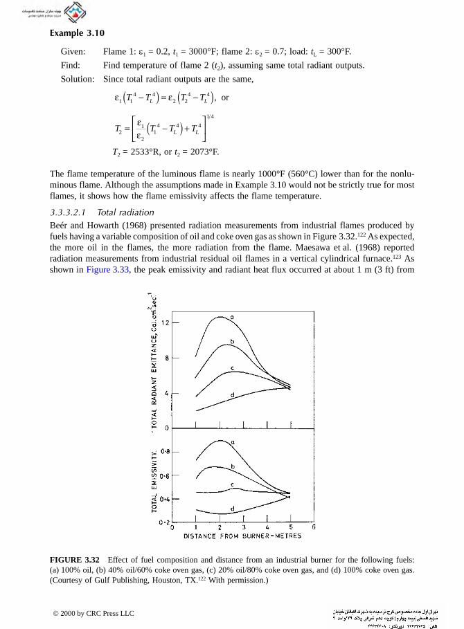
Example 3.10
Given: Flame 1: ε = 0.2, t = 3000°F; flame 2: ε = 0.7; load: t = 300°F.
1 1 2 L
Find: Find temperature of flame 2 (t2), assuming same total radiant outputs.
Solution: Since total radiant outputs are the same,
T2 = 2533°R, or t2 = 2073°F.
The flame temperature of the luminous flame is nearly 1000°F (560°C) lower than for the nonlu-minous flame. Although the assumptions made in Example 3.10 would not be strictly true for most flames, it shows how the flame emissivity affects the flame temperature.
3.3.3.2.1 Total radiationBeér and Howarth (1968) presented radiation measurements from industrial flames produced by fuels having a variable composition of oil and coke oven gas as shown in Figure 3.32.122 As expected, the more oil in the flames, the more radiation from the flame. Maesawa et al. (1968) reported radiation measurements from industrial residual oil flames in a vertical cylindrical furnace.123 As shown in Figure 3.33, the peak emissivity and radiant heat flux occurred at about 1 m (3 ft) from
FIGURE 3.32 Effect of fuel composition and distance from an industrial burner for the following fuels: (a) 100% oil, (b) 40% oil/60% coke oven gas, (c) 20% oil/80% coke oven gas, and (d) 100% coke oven gas. (Courtesy of Gulf Publishing, Houston, TX.122 With permission.)
ε ε
εε
1 14 4
2 24 4
21
21
4 4 4
1 4
T T T T
T T T T
L L
L L
−( ) = −( )
= −( ) +⎡
⎣⎢
⎤
⎦⎥
, or
© 2000 by CRC Press LLC

the burner in a 3-m (10 ft) long furnace. Gill et al. (1968) measured and predicted the radiant heat transfer from pulverized coal flames in a 6 m (20 ft) long × 1 m (3 ft) wide rectangular, water-cooled furnace.124 The peak heat flux occurred at approximately the midpoint of the furnace length. You (1985) measured the radiation from pure diffusion (φ = ×), natural gas flames.23 Much of this radiation may have been luminous for these very fuel-rich flames. Radiation to the stagnation point was 13% to 26% of the total heat flux. Radiation was negligible at the edge of the plate (R = 7.3). Hustad calculated the radiant flux to be 7% to 14% and 20% to 40% of the total flux for CH4 and C3H8 pure diffusion flames (φ = ×), respectively.37 Hustad assumed that these long flames were optically thick radiating cylinders. The convective flux was calculated using correlations for flow over a cylinder. This was subtracted from the measured total flux to determine a calculated radiant flux. This calculated radiation compared favorably with the measured radiation. The following empirical correlation was derived:
(3.52)
where q″b,rad is in kW/m2 and xliftoff is the axial distance from the nozzle exit to the start of the flame. Luminous radiation was not considered in other studies, where the flames were very fuel rich (e.g., Reference 28), although it may have been important.
FIGURE 3.33 Measured radiant heat flux and calculated flame emissivity as a function of the distance from the burner for a residual oil flame in a vertical cylindrical furnace. (Courtesy of The Combustion Institute, Pittsburgh, PA.123 With permission.)
′′ = + −( )q l xb j, .rad liftoff5 3 9
© 2000 by CRC Press LLC

3.3.3.2.2 Spectral radiationThe Ji and Baukal (1998) study discussed above also investigated luminous flame radiation.92 The increased penetrating radiation in the extreme fuel-rich case (φ = 2.00) reported above comes from the soot radiation. Incomplete combustion causes the fuel to crack, which forms soot particles at high temperatures. These hot soot particles emit blackbody-type radiation. The total radiation in this case is composed of discrete molecular band spectra (from hot combustion products) super-imposed onto a blackbody continuum (from soot particles). The continuum radiation in the φ = 2.00 flame spectra can be accounted for by a blackbody at 2318K (3713°F), which has peak radiation at 1.25 µm. Figure 3.34 decomposes the φ = 2.00 flame spectra into its soot blackbody continuum and its molecular band spectra components. The discrete band spectra are dominated by the hot combustion products: H2O bands at 1.14, 1.38, 1.87, and 2.7 µm, and CO2 bands at 2.7 and 4.3 µm. The CH4 fuel molecules (2.3 and 3.3 µm bands) and combustion intermediate CO molecules (4.7 µm band) do not make a significant contribution to the flame radiation.
For quantitative characterization of the relative contributions from soot and molecular radiation, a soot radiation index γ was defined as:
(3.53)
Since the soot blackbody radiation peaks at 1.250 µm and there is little molecular radiation at this wavelength, it was therefore assumed that:
I(soot at 1.250 µm) = I(total at 1.250 µm) (3.54)
The H2O molecular radiation has a sharp rising (band head) peak at 1.346 µm, therefore it can be approximated that:
I(molecule at 1.346 µm) = I(total at 1.346 µm) — I(soot at 1.250 µm) (3.55)
FIGURE 3.34 Soot radiation from a fuel-rich flame (φ = 2.00). (From B. Ji and C.E. Baukal, Proc. 1998 Int. Gas Research Conf., Nov. 8-11, 1998, San Diego, CA, D. Dolenc, Ed., 5, 422-433, 1998.)
γ = µ( )
µ( )
I
Isoot at 1.250 m
molecule at 1.346 m
© 2000 by CRC Press LLC

Because the Monolight spectrometer had a nearly flat response sensitivity over the narrow wave-length range from 1.250 to 1.346 µm, the value of soot radiation index γ reported here is independent of the spectrometer calibration. Table 3.5 lists the soot radiation index γ for qf = 5.0 kW flames.
Figure 3.35 shows the normalized total radiation intensity Inrm(total), the normalized penetrating radiation intensity Inrm(pen.), and the soot radiation index γ as a function of the fuel equivalence ratio (φ) for Ω = 1.00, qf = 5.0 kW flames. As φ increased to fuel rich, both Inrm(total) and Inrm(pen.) decreased first due to incomplete combustion. At φ = 1.79, Inrm(pen.) started to increase due to increased soot radiation. This increase in Inrm(pen.) corresponds to a rapid increase in the soot radiation index γ. Finally, at φ = 2.00, Inrm(total) also increased since the much increased soot radiation became a significant part of the total radiation. The soot radiation index γ correlates closely to the soot concentration in the flame. A new commercial high-radiation burner125 has a soot index of close to 4, compared to the highest value in this study, which was slightly greater than 1 (see Table 3.5).
3.4 CONDUCTION
Thermal conduction is often overlooked when considering heat transfer in combustion systems. Although it is not an important heat transfer mode in the combustion space, it is important in determining the heat loss through the refractory walls. Conduction is important in the design of furnaces because of the thermal expansion that occurs as the furnace heats up, especially considering the difference in expansion between refractories and the metal shell.126
Thermal conduction has played an important role in many flame impingement heating appli-cations. In some processes, high thermal conduction rates are desired. An example is a rapid reheat furnace. There, the goal is to raise the temperature of metal parts. Because metals generally have high thermal conductivities, heat can be quickly conducted through the part. This reduces the temperature gradient between the surface and the interior of the part. High gradients may cause
FIGURE 3.35 Normalized total radiation intensity Inrm(total), normalized penetrating radiation intensity Inrm(pen.), and soot radiation index γ as a function of fuel equivalence ratio φ for Ω = 1.00 flames. (From B. Ji and C.E. Baukal, Proc. 1998 Int. Gas Research Conf., Nov. 8-11, 1998, San Diego, CA, D. Dolenc, Ed., 5, 422-433, 1998.)
© 2000 by CRC Press LLC
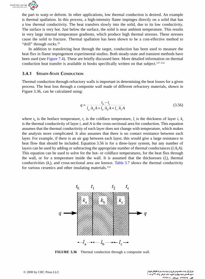
the part to warp or deform. In other applications, low thermal conduction is desired. An example is thermal spallation. In this process, a high-intensity flame impinges directly on a solid that has
a low thermal conductivity. The heat transfers slowly into the solid, due to its low conductivity. The surface is very hot. Just below the surface, the solid is near ambient temperature. This results in very large internal temperature gradients, which produce high thermal stresses. These stresses cause the solid to fracture. Thermal spallation has been shown to be a cost-effective method to “drill” through rocks.35
In addition to transferring heat through the target, conduction has been used to measure the heat flux in flame impingement experimental studies. Both steady-state and transient methods have been used (see Figure 7.4). These are briefly discussed here. More detailed information on thermal conduction heat transfer is available in books specifically written on that subject.127-132
3.4.1 STEADY-STATE CONDUCTION
Thermal conduction through refractory walls is important in determining the heat losses for a given process. The heat loss through a composite wall made of different refractory materials, shown in Figure 3.36, can be calculated using:
(3.56)
where th is the hotface temperature, tc is the coldface temperature, li is the thickness of layer i, ki
is the thermal conductivity of layer i, and A is the cross-sectional area for conduction. This equation assumes that the thermal conductivity of each layer does not change with temperature, which makes the analysis more complicated. It also assumes that there is no contact resistance between each layer. For example, if there is an air gap between each layer, this would give a large resistance to heat flow that should be included. Equation 3.56 is for a three-layer system, but any number of layers can be used by adding or subtracting the appropriate number of thermal conductances (li /ki A). This equation can be used to solve for the hot- or coldface temperatures, for the heat flux through the wall, or for a temperature inside the wall. It is assumed that the thicknesses (li), thermal conductivities (ki), and cross-sectional area are known. Table 3.7 shows the thermal conductivity for various ceramics and other insulating materials.133
FIGURE 3.36 Thermal conduction through a composite wall.
qt t
l k A l k A l k Ah c
a a b b c c
=−
+ +
© 2000 by CRC Press LLC
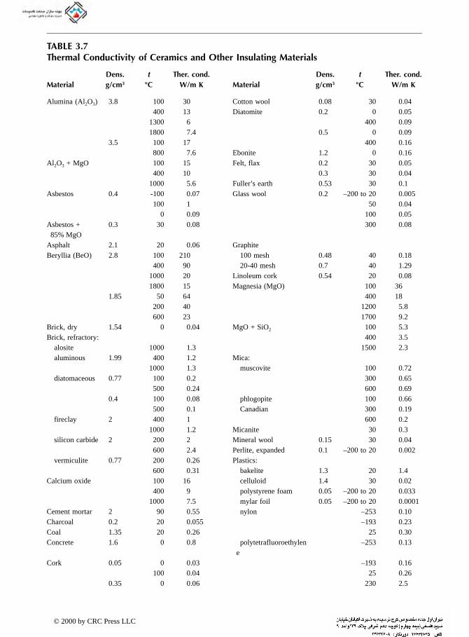
TABLE 3.7
Thermal Conductivity of Ceramics and Other Insulating Materials
Dens. t Ther. cond. Dens. t Ther. cond.Material g/cm3 °C W/m K Material g/cm3 °C W/m K
Alumina (Al2O3) 3.8 100 30 Cotton wool 0.08 30 0.04400 13 Diatomite 0.2 0 0.05
1300 6 400 0.091800 7.4 0.5 0 0.09
3.5 100 17 400 0.16800 7.6 Ebonite 1.2 0 0.16
Al2O3 + MgO 100 15 Felt, flax 0.2 30 0.05400 10 0.3 30 0.04
1000 5.6 Fuller’s earth 0.53 30 0.1Asbestos 0.4 -100 0.07 Glass wool 0.2 –200 to 20 0.005
100 1 50 0.040 0.09 100 0.05
Asbestos + 85% MgO
0.3 30 0.08 300 0.08
Asphalt 2.1 20 0.06 GraphiteBeryllia (BeO) 2.8 100 210 100 mesh 0.48 40 0.18
400 90 20-40 mesh 0.7 40 1.291000 20 Linoleum cork 0.54 20 0.081800 15 Magnesia (MgO) 100 36
1.85 50 64 400 18200 40 1200 5.8600 23 1700 9.2
Brick, dry 1.54 0 0.04 MgO + SiO2 100 5.3Brick, refractory: 400 3.5 alosite 1000 1.3 1500 2.3 aluminous 1.99 400 1.2 Mica: 1000 1.3 muscovite 100 0.72 diatomaceous 0.77 100 0.2 300 0.65
500 0.24 600 0.690.4 100 0.08 phlogopite 100 0.66
500 0.1 Canadian 300 0.19 fireclay 2 400 1 600 0.2
1000 1.2 Micanite 30 0.3 silicon carbide 2 200 2 Mineral wool 0.15 30 0.04
600 2.4 Perlite, expanded 0.1 –200 to 20 0.002 vermiculite 0.77 200 0.26 Plastics:
600 0.31 bakelite 1.3 20 1.4Calcium oxide 100 16 celluloid 1.4 30 0.02
400 9 polystyrene foam 0.05 –200 to 20 0.0331000 7.5 mylar foil 0.05 –200 to 20 0.0001
Cement mortar 2 90 0.55 nylon –253 0.10Charcoal 0.2 20 0.055 –193 0.23Coal 1.35 20 0.26 25 0.30Concrete 1.6 0 0.8 polytetrafluoroethylen
e–253 0.13
Cork 0.05 0 0.03 –193 0.16100 0.04 25 0.26
0.35 0 0.06 230 2.5
© 2000 by CRC Press LLC

TABLE 3.7 (continued)
Example 3.11
Given: Cold face temperature of 140°F, heat flux to the wall of 400 Btu/hr-ft2, 8 in. of fireclay brick.
Find: The hot face temperature.
Solution: Assume that the conductivity through the steel shell is negligible. Note that heat flux per unit area is given (q/A). Rearrange the equation above to solve for the hot face temperature:
From Table 3.7, kfirebrick = 1.1 W/m-K = 0.64 Btu/hr-ft-°F,
lfirebrick = 8/12 ft, tc = 140°F
solving for th = 557°F
100 0.08 urethane foam 0.07 20 0.06Dens. t Ther. cond. Dens. t Ther. cond.
Material g/cm3 °C W/m K Material g/cm3 °C W/m K
Porcelain 90 1 Uranium dioxide 100 9.8Rock: 400 5.5 basalt 20 2 1000 3.4 chalk 20 0.92 Wood: granite 2.8 20 2.2 balsa, ^ 0.11 30 0.04 limestone 2 20 1 fir, ^ 0.54 20 0.14 sandstone 2.2 20 1.3 fir, || 0.54 20 0.35 slate, ^ 95 1.4 oak 20 0.16 slate, || 95 2.5 plywood 20 0.11Rubber: pine, ^ 0.45 60 0.11 sponge 0.2 20 0.05 pine, || 0.45 60 0.26 92 percent 25 0.16 walnut, ^ 0.65 20 0.14Sand, dry 1.5 20 0.33 Wool 0.09 30 0.04Sawdust 0.2 30 0.06 Zinc oxide 200 17Shellac 20 0.23 800 5.3Silica aerogel 0.1 –200 to 20 0.003 Zirconia (ZrO2) 100 2Snow 0.25 0 0.16 400 2Steel wool 0.1 55 0.09 1500 2.5Thoria (ThO2) 100 10 Zirconia + silica 200 5.6
400 5.8 600 4.61500 2.4 1500 3.7
Titanium dioxide 100 6.5400 3.8
1200 3.3
Thermal conductivity values for ceramics, refractory oxides, and miscellaneous insulating materials are given here. The thermal conductivity refers to samples with density indicated in the second column. Since most of these materials are highly variable, the values should only be considered as a rough guide.
Source: From CRC Handbook of Chemistry and Physics, 79th edition, CRC Press, Boca Raton, FL, 1998, 12-191–12-192.
Thermal Conductivity of Ceramics and Other Insulating Materials
t tqA
l
kh c= + ⎛⎝⎞⎠⎛⎝⎜
⎞⎠⎟
firebrick
firebrick
© 2000 by CRC Press LLC

Steady-state conduction has been important in flame impingement studies. Internally cooled targets have been used in many of the experimental studies.15,17,19,21,26-29,31,33,34,36,89,90 The flame impinges on the hot side of the target. The coolant flows past the cold side of the target (see Figures 7.1 and 7.2). In other studies, the target has been an uncooled ceramic.11,13,14,18,27 In both the cooleds metal and uncooled ceramic studies, the hot side and cold side temperatures have been approximately constant, producing steady-state conduction through the target.
Steady-state conduction methods have been employed in the design of heat flux gages (see Chapter 6) used in flame impingement studies. These methods involve measuring the temperature gradient through a piece of metal in the gage. The gage is heated on one side by the flame. The other side is commonly maintained at a fixed temperature, using a coolant. Long thin solid rods,11,15,17,28,33,36 thin disks, and heat flux transducers, have been used as gages.
3.4.2 TRANSIENT CONDUCTION
Transient conduction is an important aspect of heat transfer in industrial combustion that is often overlooked. It is significant during start-up of a process where the heat distribution through the walls of a furnace has not reached the steady state. Figure 3.37 shows how the temperature distribution through a refractory wall changes as a function of time. At τo, the temperature through the wall is uniform (tcold), when heat is then applied to the left side of the wall. After some time (τ×), the wall temperature distribution reaches steady-state.
Another instance where transient conduction is important is during the heating of a load in a batch heating process. The load is initially cold after it first is charged into the furnace. As heat is applied to the surface, the surface temperature rises quickly, while the temperatures inside the load are still low until the heat has time to conduct through the load. The thermal conductivity of the load determines how fast the temperature profile equilibrates inside the load. For example, alumi-num conducts very quickly compared to refractory materials like bricks or ceramics. This can be an important consideration if the material conducts slowly, as the surface can be overheated before the heat has a chance to conduct inside the load. This reduces the product quality and process yield.
Uncooled metal targets have been used in previous flame impingement experimental studies (see Chapter 7). The target materials have been steel,12,18,30,37 inconel,32 iron,87 molybdenum,16
brass,20 and copper.35 These targets were exposed to the flame for only a short time. Kilham18 and Nawaz20 inserted the target into the flame for less than 1 sec. Giedt and co-workers had test durations of between 20 and 50 sec.16,87 The targets were instrumented with an array of thermocouples. The heat flux to the surface was estimated using an inverse transient heat conduction calculation. This method was discussed by Gebhart.131
FIGURE 3.37 Transient thermal conduction through a wall.
© 2000 by CRC Press LLC

Transient conduction has also been used in the design of slug calorimeter heat flux gages (see Chapter 6), as used in previous studies.18-20,32,34,36,37 Heat is received on a slug of metal inside the
calorimeter. The slug is assumed to be internally isothermal at any instant in time. The heat flux is calculated from the rise in the thermal capacitance of the slug as a function of time.
3.5 PHASE CHANGE
The three primary phase changes that can be encountered in industrial combustion applications include melting, boiling, and condensation. These are briefly discussed here.
3.5.1 MELTING
Melting involves changing the phase of a solid to a liquid. This occurs in many industrial combustion applications. Examples include melting of scrap aluminum to make aluminum alloys, melting scrap steel in the production of steel alloys, and melting of batch materials like silica used in the production of glass. Melting involves heating the solid up to the melting temperature and then supplying enough energy to change the phase from a solid to a liquid (heat of fusion):
(3.57)
where cp is the specific heat of the solid, t0 is the initial temperature of the solid, tm is the melting temperature of the solid, and hfusion is the heat of fusion of the solid. Typical melting temperatures, specific heats, and heats of fusion for various solids are given in Table 3.8.
Example 3.12
Find: From Table 3.8, the melting temperature of aluminum is 660.32°C, the specific heat is 0.897 J/g-K, and the heat of fusion is 397 J/g.
Given: Calculate how much energy is required to melt aluminum that is initially at 20°C.
Solution: The energy to heat the aluminum to the melting temperature and change it from a solid to a liquid =
q1 = cp (tm – t0) = (0.897 J/g-K) (660.32 – 20) K = 574 J/g
q2 = 397 J/g
qm = q1 + q2 = 574 + 397 = 971 J/g = 971 kJ/kg
3.5.2 BOILING
Boiling involves changing the phase of a liquid to a vapor. The most common occurrence of boiling is when the heat from the combustion process is used to vaporize a process fluid or fluid like water used to simulate the heat flux to a load. For example, both the internal and external boiling of water have been considered in previous flame impingement experimental studies (see Figure 7.7). In internal boiling, the coolant vaporizes inside the target. In external boiling, water, in the com-bustion products, vaporizes on the outside of the target. Both types are sometimes referred to as forced convection boiling.134 This refers to boiling where the flow is through a passage or over a surface. The flow is two-phase since both liquid and vapor are present. Only internal boiling has been explicitly discussed in previous impingement studies. Although not discussed in any of those studies, external boiling may have occurred in some of the previous experiments. The effects of boiling were not quantified in any study. Further information on this topic is available in books specifically devoted to boiling.135-142
q c t t hpm m= −( ) +0 fusion
© 2000 by CRC Press LLC
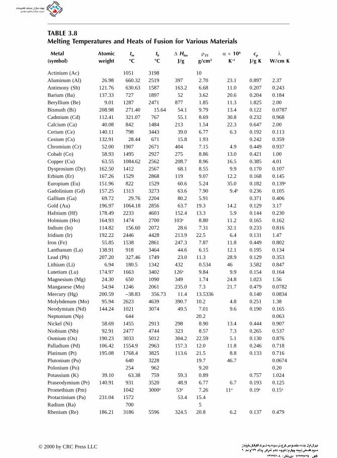
TABLE 3.8
Melting Temperatures and Heats of Fusion for Various Materials
Metal Atomic tm tb ∆ Hfus ρ25 α × 106 cp λ(symbol) weight °C °C J/g g/cm3 K–1 J/g K W/cm K
Actinium (Ac) 1051 3198 10Aluminum (Al) 26.98 660.32 2519 397 2.70 23.1 0.897 2.37Antimony (Sb) 121.76 630.63 1587 163.2 6.68 11.0 0.207 0.243Barium (Ba) 137.33 727 1897 52 3.62 20.6 0.204 0.184Beryllium (Be) 9.01 1287 2471 877 1.85 11.3 1.825 2.00Bismuth (Bi) 208.98 271.40 15.64 54.1 9.79 13.4 0.122 0.0787Cadmium (Cd) 112.41 321.07 767 55.1 8.69 30.8 0.232 0.968Calcium (Ca) 40.08 842 1484 213 1.54 22.3 0.647 2.00Cerium (Ce) 140.11 798 3443 39.0 6.77 6.3 0.192 0.113Cesium (Cs) 132.91 28.44 671 15.8 1.93 0.242 0.359Chromium (Cr) 52.00 1907 2671 404 7.15 4.9 0.449 0.937Cobalt (Co) 58.93 1495 2927 275 8.86 13.0 0.421 1.00Copper (Cu) 63.55 1084.62 2562 208.7 8.96 16.5 0.385 4.01Dysprosium (Dy) 162.50 1412 2567 68.1 8.55 9.9 0.170 0.107Erbium (Er) 167.26 1529 2868 119 9.07 12.2 0.168 0.145Europium (Eu) 151.96 822 1529 60.6 5.24 35.0 0.182 0.139a
Gadolinium (Gd) 157.25 1313 3273 63.6 7.90 9.4b 0.236 0.105Gallium (Ga) 69.72 29.76 2204 80.2 5.91 0.371 0.406Gold (Au) 196.97 1064.18 2856 63.7 19.3 14.2 0.129 3.17Hafnium (Hf) 178.49 2233 4603 152.4 13.3 5.9 0.144 0.230Holmium (Ho) 164.93 1474 2700 103a 8.80 11.2 0.165 0.162Indium (In) 114.82 156.60 2072 28.6 7.31 32.1 0.233 0.816Iridium (Ir) 192.22 2446 4428 213.9 22.5 6.4 0.131 1.47Iron (Fe) 55.85 1538 2861 247.3 7.87 11.8 0.449 0.802Lanthanum (La) 138.91 918 3464 44.6 6.15 12.1 0.195 0.134Lead (Pb) 207.20 327.46 1749 23.0 11.3 28.9 0.129 0.353Lithium (Li) 6.94 180.5 1342 432 0.534 46 3.582 0.847Lutetium (Lu) 174.97 1663 3402 126a 9.84 9.9 0.154 0.164Magnesium (Mg) 24.30 650 1090 349 1.74 24.8 1.023 1.56Manganese (Mn) 54.94 1246 2061 235.0 7.3 21.7 0.479 0.0782Mercury (Hg) 200.59 –38.83 356.73 11.4 13.5336 0.140 0.0834Molybdenum (Mo) 95.94 2623 4639 390.7 10.2 4.8 0.251 1.38Neodymium (Nd) 144.24 1021 3074 49.5 7.01 9.6 0.190 0.165Neptunium (Np) 644 20.2 0.063Nickel (Ni) 58.69 1455 2913 298 8.90 13.4 0.444 0.907Niobium (Nb) 92.91 2477 4744 323 8.57 7.3 0.265 0.537Osmium (Os) 190.23 3033 5012 304.2 22.59 5.1 0.130 0.876Palladium (Pd) 106.42 1554.9 2963 157.3 12.0 11.8 0.246 0.718Platinum (Pt) 195.08 1768.4 3825 113.6 21.5 8.8 0.133 0.716Plutonium (Pu) 640 3228 19.7 46.7 0.0674Polonium (Po) 254 962 9.20 0.20Potassium (K) 39.10 63.38 759 59.3 0.89 0.757 1.024Praseodymium (Pr) 140.91 931 3520 48.9 6.77 6.7 0.193 0.125Promethium (Pm) 1042 3000a 53a 7.26 11a 0.19a 0.15a
Protactinium (Pa) 231.04 1572 53.4 15.4Radium (Ra) 700 5Rhenium (Re) 186.21 3186 5596 324.5 20.8 6.2 0.137 0.479
© 2000 by CRC Press LLC

TABLE 3.8 (continued)
3.5.2.1 Internal Boiling
One example of internal boiling has been inside targets heated by flame impingement. Kilham and co-workers used targets that were cooled by glycol to prevent boiling inside the targets.15,17,33,36
Rajani used a water-cooled steel disk as a target.31 The target surface temperature was estimated to be 400 to 480°F (200 to 250°C). Calculations showed that boiling inside the target was probable, based on the expected heat flux rates. To prevent boiling, internal fins were added in the cooling passages. This increased both the internal surface area and the turbulence level of the cooling water flow. Both of these factors increased the effective convective heat transfer coefficient inside the target. Then, the calculated convection coefficient was high enough to preclude boiling in the target. However, no measurements were made to determine if boiling did occur.
3.5.2.2 External Boiling
External boiling is important in many processes involving drying of a material, particularly a surface. For example, removing water from the surface of wet metal scrap material can involve external boiling to vaporize the free moisture. This occurs during the initial heating phase of scrap melting processes, such as steel or aluminum, when the scrap is wet from recent rain. This moisture
Rhodium (Rh) 102.91 1964 3695 258.4 12.4 8.2 0.243 1.50Rubidium (Rb) 85.47 39.31 688 25.6 1.53 0.363 0.582Ruthenium (Ru) 101.07 2334 4150 381.8 12.1 6.4 0.238 1.17Samarium (Sm) 150.36 1074 1794 57.3 7.52 12.7 0.197 0.133Scandium (Sc) 44.96 1541 2836 314 2.99 10.2 0.568 0.158Silver (Ag) 107.87 961.78 2162 104.8 10.5 18.9 0.235 4.29Sodium (Na) 22.99 97.72 883 113 0.97 71 1.228 1.41Strontium (Sr) 87.62 777 1382 84.8 2.64 22.5 0.301 0.353Tantalum (Ta) 180.95 3017 5458 202.1 16.4 6.3 0.140 0.575Technetium (Tc) 2157 4265 11 0.506Terbium (Tb) 158.93 1356 3230 67.9 8.23 10.3 0.182 0.111Thallium (Tl) 204.38 304 1473 20.3 11.8 29.9 0.129 0.461Thorium (Th) 232.04 1750 4788 59.5 11.7 11.0 0.113 0.540Thulium (Tm) 168.93 1545 1950 99.4 9.32 13.3 0.160 0.169Tin (Sn) 118.71 231.93 2602 59.2 7.26 22.0 0.228 0.666Titanium (Ti) 47.88 1668 3287 295 4.51 8.6 0.523 0.219Tungsten (W ) 183.84 3422 5555 284.5 19.3 4.5 0.132 1.74Uranium (U) 238.03 1135 4131 38.4 19.1 13.9 0.116 0.276Vanadium (V) 50.94 1910 3407 422 6.0 8.4 0.489 0.307Ytterbium (Yb) 173.04 819 1196 44.3 6.90 26.3 0.155 0.385Yttrium (Y) 88.91 1522 3345 128 4.47 10.6 0.298 0.172Zinc (Zn) 65.39 419.53 907 112 7.14 30.2 0.388 1.16Zirconium (Zr) 91.22 1855 4409 230 6.52 5.7 0.278 0.227
a Estimated.b At 100°C.
Source: Courtesy of CRC Press, Boca Raton, FL.133
Melting Temperatures and Heats of Fusion for Various Materials
Metal Atomic tm tb ∆ Hfus ρ25 α × 106 cp λ(symbol) weight °C °C J/g g/cm3 K–1 J/g K W/cm K
© 2000 by CRC Press LLC
vaporization can represent a large additional heat load to the process that may vary from day to day and from season to season depending on the weather. This mechanism has not been discussed
in any of the previous flame impingement studies although it may have been present. Kilham and Purvis18 and Nawaz20 studied O2 /CH4 flames. The combustion products should have been about 67% water vapor by volume. These flames impinged normal to the nose of an uncooled, stainless steel, hemi-nosed cylinder. The cylinder was inserted into the flame with a solenoid. The temperature rise of the cylinder, as a function of time, was recorded. The heat flux was determined by calculating the rate of temperature rise, in the range between about 63°F and 300°F (17°C and 150°C). Because of the high concentration of water in the impinging gases, some of the water may have condensed on the target when it was below 212°F (100°C). The condensed water may then have boiled off the target, as its temperature increased above 212°F (100°C). The boiling would have been in the temperature range that was used to calculate the heat flux. If boiling was important, there may have been a plateau in the temperature curves (which were not given), near 212°F (100°C). Rauenzahn studied stoichiometric, turbulent O2 /C3H8 flames impinging on an uncooled copper slab.35 The measured slab surface temperature ranged from 63°F to 410°F (17°C to 210°C). The combustion products should have been about 57% water by volume. Again, that water may have condensed on the target when the surface temperature was below 212°F (100°C), and then subse-quently boiled off when the surface temperature increased above 212°F (100°C).
3.5.3 CONDENSATION
Condensation involves converting a vapor to a liquid. This is not often encountered in industrial combustion applications. However, it has been used in some flame impingement studies that attempted to determine the heat flux to a simulated load (see Figure 7.8). Kilham and co-workers used targets internally cooled by ethylene glycol.15,17,33,36 The target surface temperature was main-tained above the boiling point of water (212°F [100°C]) and below that of the glycol (388°F [198°C]). This prevented the water in the combustion products from condensing on the outside of the target. It also prevented the glycol from boiling inside the target. Water-cooled targets have been used in many studies.21,26-29,34,89,90 The target surface temperature has commonly been main-tained below 212°F (100°C) to prevent the cooling water from boiling inside the target. However, the water in the combustion products may have condensed on the outside of the target. Such condensation heat transfer effects were not considered in those studies. For air/fuel flames, the water content in the combustion products is only about 18% by volume. However, in O2 /CH4 flames, for example, the combustion products may contain up to 67% water by volume. Condensation may be important in any study (e.g., Reference 18) where O2 is the oxidizer, and where the target surface temperature is below 212°F (100°C).
REFERENCES
1. T.M. Smith, private communication, 1982.2. V.S. Arpaci, Convection Heat Transfer, Prentice-Hall, Englewood Cliffs, NJ, 1984.3. C.S. Fang, Convective Heat Transfer, Gulf Publishing, Houston, TX, 1985.4. S. Kakac, R.K. Shah, and W. Aung, Eds., Handbook of Single-Phase Convective Heat Transfer, Wiley,
New York, 1987.5. L.C. Burmeister, Convective Heat Transfer, 2nd edition, Wiley, New York, 1993.6. W.M. Kays and M.E. Crawford, Convective Heat and Mass Transfer, 3rd edition, McGraw-Hill, New
York, 1993.7. A. Bejan, Convection Heat Transfer, 2nd edition, Wiley, New York, 19948. M. Kaviany, Principles of Convective Heat Transfer, Springer-Verlag, New York, 1994.9. S. Kakac and Y. Yener, Convective Heat Transfer, 2nd edition, CRC Press, Boca Raton, FL, 1995.
10. P.H. Oosthuizen, An Introduction to Convective Heat Transfer, McGraw-Hill, New York, 1999.
© 2000 by CRC Press LLC
11. J.M. Beér and N.A. Chigier, Impinging jet flames, Comb. Flame, 12, 575-586, 1968.12. A. Milson and N.A. Chigier, Studies of methane-air flames impinging on a cold plate, Comb. Flame,
21, 295-305, 1973.
13. E.G. Jackson and J.K. Kilham, Heat transfer from combustion products by forced convection, Ind. Eng. Chem., 48(11), 2077-2079, 1956.
14. J.K. Kilham, Energy transfer from flame gases to solids, Third Symposium on Combustion and Flame and Explosion Phenomena, The Williams and Wilkins Co., Baltimore, MD, 1949, 733-740.
15. R.A. Cookson and J.K. Kilham, Energy transfer from hydrogen-air flames, Ninth Symposium (Inter-national) on Combustion, Academic Press, New York, 1963, 257-263.
16. L.W. Woodruff and W.H. Giedt, Heat transfer measurements from a partially dissociated gas with high Lewis number, J. Heat Transfer, 88, 415-420, 1966.
17. J.K. Kilham and P.G. Dunham, Energy transfer from carbon monoxide flames, Eleventh Symposium (International) on Combustion, The Combustion Institute, Pittsburgh, PA, 1967, 899-905.
18. J.K. Kilham and M.R.I. Purvis, Heat transfer from hydrocarbon-oxygen flames, Comb. Flame, 16, 47-54, 1971.
19. R. Conolly and R.M. Davies, A study of convective heat transfer from flames, Int. J. Heat Mass Transfer, 15, 2155-2172, 1972.
20. S. Nawaz, Heat Transfer from Oxygen Enriched Methane Flames, Ph.D. thesis, The University of Leeds, Leeds, U.K., 1973.
21. C.J. Hoogendoorn, C.O. Popiel, and T.H. van der Meer, Turbulent heat transfer on a plane surface in impingement round premixed flame jets, Proc. of 6th Int. Heat Trans. Conf., Toronto, 4, 107-112, 1978.
22. J.K. Kilham and M.R.I. Purvis, Heat transfer from normally impinging flames, Comb. Sci. Tech., 18, 81-90, 1978.
23. H.-Z. You, An investigation of fire-plume impingement on a horizontal ceiling: 2. Impingement and ceiling-jet regions, Fire & Materials, 9(l), 46-56, 1985.
24. M. Sibulkin, Heat transfer near the forward stagnation point of a body of revolution, J. Aero. Sci., 19, 570-571, 1952.
25. C.E. Baukal and B. Gebhart, A review of semi-analytical solutions for flame impingement heat transfer, Int. J. Heat Mass Transfer, 39(14), 2989-3002, 1996.
26. S.N. Shorin and V.A. Pechurkin, Effectivnost’ teploperenosa na poverkhnost’ plity ot vysokotemperaturnoi strui produktov sjoraniya razlichnykh gazov, Teoriya i Praktika Szhiganiya Gaza, 4, 134-143, 1968.
27. J.-P. Vizioz and T.M. Lowes, Convective Heat Transfer from Impinging Flame Jets, Int’l Flame Res. Found. Report F 35/a/6, IJmuiden, The Netherlands, 1971.
28. E. Buhr, G. Haupt, and H. Kremer, Heat transfer from impinging turbulent jet flames to plane surfaces, Combustion Institute European Symposium 1973, F.J. Weinberg, Ed., Academic Press, New York, 1973, 607-612.
29. R.B. Smith and T.M. Lowes, Convective Heat Transfer from Impinging Tunnel Burner Flames — A Short Report on the NG-4 Trials, Int. Flame Res. Found. Report F 35/a/9, IJmuiden, The Netherlands, 1974.
30. M. Matsuo, M. Hattori, T. Ohta and S. Kishimoto, The Experimental Results of the Heat Transfer by Flame Impingement, Int. Flame Res. Found. Report F 29/1a/1, IJmuiden, The Netherlands, 1978.
31. J.B. Rajani, R. Payne and S. Michelfelder, Convective Heat Transfer from Impinging Oxygen–Natural Gas Flames. Experimental Results from the NG5 Trials, Int. Flame Res. Found. Report F 35/a/12, IJmuiden, The Netherlands, 1978.
32. A. Ivernel and P. Vernotte, Etude expérimentale de l’amélioration des transferts convectis dans les fours par suroxygénation du comburant, Rev. Gén. Therm., Fr., Nos. 210-211, pp. 375-391, 1979.
33. G.K. Hargrave and J.K. Kilham, The Effect of Turbulence Intensity on Convective Heat Transfer From Premixed Methane-Air Flames, Inst. Chem. Eng. Symp. Ser., 2(86), 1025-1034, 1984.
34. M.E. Horsley, M.R.I. Purvis, and A.S. Tariq, Convective heat transfer from laminar and turbulent premixed flames, Heat Transfer 1982, U. Grigull, E. Hahne, K. Stephen, and J. Straub, Eds., Hemi-sphere, Washington, D.C., 3, 409-415, 1982.
35. R.M. Rauenzahn, Analysis of Rock Mechanics and Gas Dynamics of Flame-Jet Thermal Spallation Drilling, Ph.D. thesis, MIT, Cambridge, MA, 1986.
36. G.K. Hargrave, M. Fairweather, and J.K. Kilham, Forced convective heat transfer from premixed flames. 2. Impingement heat transfer, Int. J. Heat Fluid Flow, 8(2), 132-138, 1987.
© 2000 by CRC Press LLC

37. J.E. Hustad and O.K. Sønju, Heat transfer to pipes submerged in turbulent jet diffusion flames, in Heat Transfer in Radiating and Combusting Systems, Springer-Verlag, Berlin, 1991, 474-490.
38. T.H. van der Meer, Stagnation point heat transfer from turbulent low Reynolds number jets and flame
jets, Exper. Therm. Fluid Sci., 4, 115-126, 1991.39. V.I. Babiy, Solid/gas phase heat exchange in combustion of powdered fuel, in Heat Transfer in Flames,
N.H. Afgan and J.M. Beer, Eds., Scripta Book Company, Washington, D.C., 1974, chap. 7, 131-139.40. J. Griswold, Fuels, Combustion, and Furnaces, McGraw-Hill, New York, 1946.41. C.C. Monrad, Heat Transmission in Convection Sections of Pipe Stills, Ind. Eng. Chem., 24, 505-509,
1932.42. B. Gebhart, Y. Jaluria, R. Mahajan, and B. Sammakia, Buoyancy-Induced Flows and Transport,
Hemisphere, New York, 1988.43. Y.B. Wang, C. Chaussavoine, and F. Teyssandier, Two-dimensional modelling of a non-confined
circular impinging jet reactor — fluid dynamics and heat transfer, Int. J. Heat Mass Trans., 36(4), 857-873, 1993.
44. G.M. Faeth, J.P. Gore, S.G. Chuech, and S.-M. Jeng, Radiation from turbulent diffusion flames, Annu. Rev. of Fluid Mech. Heat Transfer, 2, 1-38, 1989.
45. W.A. Gray and R. Müller, Engineering Calculations in Radiative Heat Transfer, Pergamon, Oxford, U.K., 1974.
46. B. Leblanc and E. Goracci, Example of applications in the field of heat transfer in hot wall furnaces, La Rivista dei Combustibili, 27(4-5), 155-164, 1973.
47. H. Schmidt, Prüfung der Strahlungsgesetze der Bunsenflamme, Annln. Phys., 29, 971-1028, 1909.48. T.M. Lowes and A.J. Newall, Problems associated with the characterisation (sic) of flame radiation
in glass tanks, Glass Tech., 12(2), 32-35, 1971.49. B. Leblanc, A.B. Ivernel, and J. Chedaille, New concepts on heat transfer processes in high temperature
furnaces, Heat transfer, Proceedings of International Heat Transfer Conference, 5th, Vol. 1, Japanese Soc. Mech. Eng., Tokyo, 1974, 61-65.
50. D.A. Lihou, Review of furnace design methods, Trans. IChemE, 55(4), 225-242, 1977.51. J.A. Wiebelt, Engineering Radiation Heat Transfer, Holt, Rinehart and Winston, New York, 1966.52. H.C. Hottel and A.F. Sarofim, Radiative Transfer, McGraw-Hill, New York, 1967.53. T.J. Love, Radiative Heat Transfer, Merrill Publ., Columbus, OH, 1968.54. E.M. Sparrow and R.D. Cess, Radiation Heat Transfer, augmented edition, Hemisphere, Washington,
D.C., 1978.55. D.K. Edwards, Radiation Heat Transfer Notes, Hemisphere, Washington, D.C., 1981.56. R. Siegel and J.R. Howell, Thermal Radiation Heat Transfer, Second Edition, Hemisphere, Washing-
ton, D.C., 1981.57. M.Q. Brewster, Thermal Radiative Transfer and Properties, Wiley, New York, 1992.58. M.F. Modest, Radiative Heat Transfer, McGraw-Hill, New York, 1993.59. D.H. Hubble, Steel plant refractories, in The Making, Shaping and Treating of Steel, 11th edition,
Steelmaking and Refining Volume, R.J. Fruehan, Ed., AISE Steel Foundation, Pittsburgh, PA, 1998, 159-290.
60. M.A. Glinkov, Flame as a problem of the general theory of furnaces, in Heat Transfer in Flames, N.H. Afgan and J.M. Beer, Eds., Scripta Book Company, Washington, D.C., 1974, chap. 9, 159-177.
61. P. Docherty and R.J. Tucker, The influence of wall emissivity on furnace performance, J. Inst. Energy, 59(438), 35-37, 1986.
62. D.G. Elliston, W.A. Gray, D.F. Hibberd, T.-Y. Ho, and A. Williams, The effect of surface emissivity on furnace performance, J. Inst. Energy, 60(445), 155-167, 1987.
63. C.L. DeBellis, Effect of refractory emittance in industrial furnaces, in Fundamentals of Radiation Heat Transfer, W.A. Fiveland, A.L. Crosbie, A.M. Smith, and T.F. Smith, Eds., ASME HTD-Vol. 160, New York, 1991, 105-115.
64. C.L. DeBellis, Evaluation of high-emittance coatings in a large industrial furnace, in Heat Transfer in Fire and Combustion Systems — 1993, B. Farouk, M.P. Menguc, R. Viskanta, C. Presser, and S. Chellaiah, Eds., New York, ASME HTD-Vol. 250, 1993, 190-198.
65. X. Xin, G. Qingchang, and J. Yi, High emissivity refractory coating improves furnace output in China, Industrial Heating, LXVI(6), 49-50, 1999.
© 2000 by CRC Press LLC

66. T.F. Wall, S.P. Bhattacharya, D.K. Zhang, R.P. Gupta, and X. He, The properties and thermal effects of ash deposits in coal fired furnaces, Prog. Energy Combust. Sci., 19, 487-504, 1993.
67. T.F. Wall, S.P. Bhattacharya, L.L. Baxter, G. Richards, and J.N. Harb, The character of ash deposits
and the thermal performance of furnaces, Fuel Processing Technology, 44, 143-153, 1995.68. W.E. Garner, Radiant energy from flames, First Symposium (International) on Combustion, The
Combustion Institute, Pittsburgh, PA, 1965, 19-23.69. A.F. Sarofim, Radiative heat transfer in combustion: friend or foe, Hoyt C. Hottel Plenary Lecture,
Twenty-First Symp. (Int.) on Combustion, The Combustion Institute, Pittsburgh, PA, 1986, 1-23.70. C.B. Ludwig, W. Malkmus, J.E. Reardon, and J.A.L. Thomson, Handbook of Infrared Radiation from
Combustion Gases, National Aeronautics and Space Administration Report SP-3080, Washington, D.C., 1973.
71. B. Leckner, Spectral and total emissivity of water vapor and carbon dioxide, Comb. Flame, 19, 33-48, 1972.72. M. Gulic, A new formula for determining the effective beam length of gas layer or flame, in Heat
Transfer in Flames, N.H. Afgan and J.M. Beer, Eds., Scripta Book Company, Washington, D.C., 1974, chap. 12, 201-208.
73. R.D. Cess, Infrared gaseous radiation, in Heat Transfer in Flames, N.H. Afgan and J.M. Beer, Eds., Scripta Book Company, Washington, D.C., 1974, chap. 15, 231-248.
74. R. Grief, Experimental and theoretical results with infrared radiating gases, in Heat Transfer in Flames, N.H. Afgan and J.M. Beer, Eds., Scripta Book Company, Washington, D.C., 1974, chap. 16, 249-253.
75. J.L. Kovotny, The effect of pressure on heat transfer in radiating gases, in Heat Transfer in Flames, N.H. Afgan and J.M. Beer, Eds., Scripta Book Company, Washington, D.C., 1974, chap. 17, 255-269.
76. D.K. Edwards, Molecular gas band radiation, in Advances in Heat Transfer, Vol. 12, T.F. Irvine and J.P. Hartnett, Eds., Academic Press, New York, 1976, 115-193.
77. H.E. Trout, Heat transfer. IV. Radiation from gases and flames, Industrial Heating, Vol. XLIV, No. 8, 28-33, 1977.
78. C.L. Tien, Thermal Radiation Properties of Gases, Advances in Heat Transfer, T.F. Irvine and J.P. Hartnett, Eds., Academic Press, New York, 5, 253-324, 1968.
79. C.L. Tien and S.C. Lee, Flame Radiation, Prog. Energy Combust. Sci., 8, 41-59, 1982.80. D.K. Edwards and A. Balakrishnan, Thermal radiation by combustion gases, Int. J. Heat Mass Transfer,
16, 25-40, 1973.81. P.B. Taylor and P.J. Foster, The total emissivities of luminous and non-luminous flames, Int. J. Heat
Mass Transfer, 17, 1591-1605, 1974.82. A. Coppalle and P. Vervisch, The total emissivities of high-temperature flames, Combust. Flame, 49,
101-108, 1983.83. D.K. Edwards and R. Matavosian, Scaling rules for total absorptivity and emissivity of gases, J. Heat
Transfer, 106, 684-689, 1984.84. J.R. Howell, Thermal radiation in participating media: the past, the present, and some possible futures,
J. Heat Transf., 110, 1220-1229, 1988.85. J.A. Wieringa, J.J. Ph. Elich, and C.J. Hoogendoorn, Spectral effects of radiative heat-transfer in high-
temperature furnaces burning natural gas, J. Inst. Energy, 63(456), 101-108, 1990.86. P.G. Dunham, Convective Heat Transfer from Carbon Monoxide Flames, Ph.D. thesis, The University
of Leeds, Leeds, U.K., 1963.87. W.H. Giedt, L.L. Cobb, and E.J. Russ, Effect of Hydrogen Recombination on Turbulent Flow Heat
Transfer, ASME Paper 60-WA-256, New York, 1960.88. M.R.I. Purvis, Heat Transfer from Normally Impinging Hydrocarbon Oxygen Flames to Surfaces at
Elevated Temperatures, Ph.D. thesis, The University of Leeds, Leeds, U.K., 1974.89. D.R. Davies, Heat Transfer from Working Flame Burners, B.S. thesis, Univ. of Salford, Salford, U.K.,
1979.90. T.H. van der Meer, Heat Transfer from Impinging Flame Jets, Ph.D. thesis, Technical University of
Delft, the Netherlands, 1987.91. C.E. Baukal and B. Gebhart, Oxygen-enhanced/natural gas flame radiation, Int. J. Heat Mass Transfer,
44(11), 2539-2547, 1997.92. B. Ji and C.E. Baukal, Spectral radiation properties of oxygen-enhanced/natural gas flames, Proc.
1998 International Gas Research Conference, 8-11 November 1998, San Diego, CA, Dan Dolenc, Ed., 5, 422-433, 1998.
© 2000 by CRC Press LLC
93. D.R. Davies and P.J.,Young, Strip Edge Heating Burner, U.S. Patent 4,756,685, issued July 12, 1988.94. C.E. Baukal, Heat Transfer from Flames Impinging Normal to a Plane Surface, Ph.D. thesis, Univ.
of Pennsylvania, 1996.
95. W. R. Anderson, Measurement of the Line Reversal Temperature of OH in CH4/N2O Flames, Technical Report ARBRL-TR-02280, 1981.
96. S. Yagi and H. Iino, Radiation from soot particles in luminous flames, Eighth Symposium (Interna-tional) on Combustion, The Combustion Institute, Pittsburgh, PA, 1961 (reprinted 1991), 288-293.
97. R. Echigo, N. Nishiwaki and M. Hirata, A study on the radiation of luminous flames, Eleventh Symposium (International) on Combustion, The Combustion Institute, Pittsburgh, PA, 1967, 381-389.
98. W.A. Gray, J.K. Kilham, and R. Müller, Heat Transfer from Flames, Elek Science, London, 1976.99. H.G. Wagner, Soot Formation in Combustion, Seventeenth Symposium (International) on Combustion,
The Combustion Institute, Pittsburgh, PA, 1978, 3-19.100. I. Glassman, Soot Formation in Combustion Processes, Twenty-Second Symposium (International) on
Combustion, The Combustion Institute, Pittsburgh, PA, 1988, 295-311.101. E. Talmor, Combustion Hot Spot Analysis for Fired Process Heaters, Gulf Publishing, Houston, TX, 1982.102. B.S. Haynes, Soot and Hydrocarbons in Combustion, in Fossil Fuel Combustion, W. Bartok and A.F.
Sarofim, Eds., Wiley, New York, 1991, chap. 5.103. P.B. Sunderland, S. Mortazavi, G.M. Faeth, and D.L. Urban, Laminar smoke points of nonbuoyant
jet diffusion flames, Combust. Flame, 96, 97-103, 1994.104. J. Lahaye and G. Prado, Eds., Soot in Combustion Systems and its Toxic Properties, Plenum Press,
New York, 1983.105. J.P. Longwell, Polycyclic aromatic hydrocarbons and soot, in Soot in Combustion Systems and its
Toxic Properties, J. Lahaye and G. Prado Eds., Plenum Press, New York, 1983, 37-56.106. J.B. Howard and J.D. Bittner, Structure of Sooting Flames, in Soot in Combustion Systems and its
Toxic Properties, J. Lahaye and G. Prado Eds., Plenum Press, New York, 1983, 57-93.107. J.D. Bittner, J.B. Howard, and H.B. Palmer, Chemistry of intermediate species in the rich combustion
of benzene, in Soot in Combustion Systems and its Toxic Properties, J. Lahaye and G. Prado Eds., Plenum Press, New York, 1983, 95-125.
108. G. Prado, J. Lahaye, and B.S. Haynes, Soot Particle Nucleation and Agglomeration, in Soot in Combustion Systems and its Toxic Properties, J. Lahaye and G. Prado Eds., Plenum Press, New York, 1983, 145-161.
109. H.F. Calcote, Ionic mechanisms of soot formation, in Soot in Combustion Systems and its Toxic Properties, J. Lahaye and G. Prado Eds., Plenum Press, New York, 1983, 197-215.
110. A.G. Blokh, Heat Transfer in Steam Boiler Furnaces, Hemisphere, Washington, D.C., 1988.111. A. Stambuleanu, Flame Combustion Processes in Industry, Abacus Press, Tunbridge Wells, U.K., 1976.112. A. Blokh, The problem of flame as a disperse system, in Heat Transfer in Flames, N.H. Afgan and
J.M. Beer, Eds., Scripta Book Company, Washington, D.C., 1974, chap. 6, 111-130.113. T. Kunitomo, Luminous flame emission under pressure up to 20 atm, in Heat Transfer in Flames,
N.H. Afgan and J.M. Beer, Eds., Scripta Book Company, Washington, D.C., 1974, chap. 18, 271-281.114. E.G. Hammond and J.M. Beér, Spatial Distribution of Spectral Radiant Energy in a Pressure Jet Oil
Flame, in Heat Transfer in Flames, N.H. Afgan and J.M. Beer, Eds., Scripta Book Company, Wash-ington, D.C., 1974, chap. 19, 283-291.
115. J.C. Ku and K-H Shim, The effects of refractive indices, size distribution, and agglomeration on the diagnostics and radiative properties of flame soot particles, in Heat and Mass Transfer in Fires and Combustion Systems, W.L. Grosshandler and H.G. Semerjian, Eds., New York, ASME HTD-Vol. 148, 1990, 105-115.
116. H. Bockhorn, Ed., Soot Formation in Combustion, Springer-Verlag, Berlin, 1994.117. A.A. Fridman, S.A. Nestor and A.V. Saveliev, Effect of pyrene addition on the luminosity of methane
flames, in ASME Proceedings of the 32nd National Heat Transfer Conf., Vol. 3: Fire and Combustion, L. Gritzo and J.-P. Delplanque, Eds., ASME, New York, 1997, 7-12.
118. T.L. Farias, M.G. Carvalho, and Ü.Ö. Köylü, Radiative heat transfer in soot-containing combustion systems with aggregation, Int. J. Heat Mass Trans., 41(17), 2581-2587, 1998.
119. M. Jacob, Heat Transfer, Vol. 2, Wiley, New York, 1957.120. W.H. McAdams, Heat Transmission, McGraw-Hill, New York, 1954.
© 2000 by CRC Press LLC
121. H.C. Hottel and F.P. Broughton, Determination of true temperature and total radiation from luminous gas flames, Ind. Eng. Chem., 4, 166-175, 1933.
122. J.M. Beér and C.R. Howarth, Radiation from flames in furnaces, Twelfth Symposium (International)
on Combustion, The Combustion Institute, Pittsburgh, PA, 1968, 1205-1217.123. M. Maesawa, Y. Tanaka, Y. Ogisu, and Y. Tsukamoto, Radiation from the luminous flames of liquid
fuel jets in a combustion chamber, Twelfth Symposium (International) on Combustion, The Combustion Institute, Pittsburgh, PA, 1968, 1229-1237.
124. D.W. Gill, D.J. Loveridge, and G.G. Thurlow, A comparison of predicted and measured heat-transfer rates in a pulverized-coal-fired furnace, Twelfth Symposium (International) on Combustion, The Combustion Institute, Pittsburgh, PA, 1968, 1239-1246.
125. A.G. Slavejkov, T.M. Gosling, and R.E. Knorr, Method and Device for Low-NOx High Efficiency Heating in High Temperature Furnace. U.S. Patent 5,575,637, 1996.
126. J.D. Gilchrist, Fuels, Furnaces and Refractories, Pergamon Press, Oxford, U.K., 1977.127. V.S. Arpaci, Conduction Heat Transfer, Addison-Wesley, Reading, MA, 1966.128. M.N. Özisik, Boundary Value Problems of Heat Conduction, Dover, New York, 1968.129. U. Grigull and H. Sandner, Heat Conduction, Hemisphere, Washington, D.C., 1984.130. G.E. Myers, Analytical Methods in Conduction Heat Transfer, Genium Publishing, Schenectady, NY,
1987.131. B. Gebhart, Heat Transfer and Mass Diffusion, McGraw-Hill, New York, 1993.132. D. Poulikakos, Conduction Heat Transfer, Prentice-Hall, Englewood Cliffs, NJ, 1994.133. D.R. Lide, Ed., CRC Handbook of Chemistry and Physics, 79th edition, CRC Press, Boca Raton, FL,
1998.134. W.M. Rohsenow, Boiling, in Handbook of Heat Transfer Fundamentals, second edition, W.M. Rohse-
now, J.P. Hartnett, and E.N. Ganic, Eds., McGraw-Hill, New York, 1985.135. S.V. Stralen and R. Cole, Eds., Boiling Phenomena, Vol. 1, Hemisphere, Washington, D.C., 1979.136. J.R. Thome, Enhanced Boiling Heat Transfer, Hemisphere, Washington, D.C., 1990.137. R.T. Lahey, Ed., Boiling Heat Transfer: Modern Developments and Advances, Elsevier, New York,
1992.138. K. Stephen, Heat Transfer in Condensation and Boiling, Springer-Verlag, 1992.139. J.G. Collier and J.R. Thome, Convective Boiling and Condensation, 3rd edition, Oxford University
Press, Oxford, U.K., 1996.140. L.S. Tong and Y.S. Tang, Boiling Heat Transfer and Two-Phase Flow, 2nd edition, Taylor & Frances,
Bristol, PA, 1997.141. S.G. Kandlikar, M. Shoji, and V.K. Dhir, Eds., Handbook of Phase Change: Boiling and Condensation,
Hemisphere, Washington, D.C., 1999.142. M. Lehner and F. Mayinger, Convective Flow and Pool Boiling, Taylor & Francis, Bristol, PA, 1999.
© 2000 by CRC Press LLC
Heat Sources and Sinks
0-8493-7686-6/97/$0.00+$.50© 1997 by CRC Press LLC
44.1 HEAT SOURCES
The primary objective of industrial heating and melting processes is to supply energy in the form of heat to some type of load. There are several possibilities for the source of that energy. In this book, only energy produced through combustion processes is considered.
4.1.1 COMBUSTIBLES
There are two general kinds of combustibles that are sources of energy in industrial combustion processes. The source that is present in every system considered in this book is the fuel supplied through the burner. A second source that may be present in a limited number of applications is volatiles coming out of the material being heated. These are briefly considered next.
4.1.1.1 Fuel Combustion
The primary source of energy in industrial heating and melting systems is from the combustion of a fossil fuel. Although electrical heating elements are used in some limited applications, this is a relatively small portion of the overall industrial sector. The overall fuel combustion reaction may be written as:
fuel + oxidizer → combustion products + heat
In this book, the transfer of that generated heat to both the load and to the combustor are of interest. The fuel and the oxidizer are generally supplied through one or more burners that produce the desired flame shape and heat transfer rates to the load.
The fuels may be solids (e.g., coal or coke), liquids (e.g., no. 2 fuel oil), gaseous (e.g., natural gas or propane), or some combination of these (e.g., natural gas and no. 2 fuel oil). Table 4.1 shows a comparison of heating values for various fuels on a weight basis. Most of those shown have higher or gross heating values of approximately 20,000 Btu/lb (47 MJ/kg), even for liquid and gaseous fuels. Hydrogen has a much higher heating value by weight, while carbon monoxide has a much lower heating value. There are many factors that may be considered when selecting the fuel for a given application including: operating costs, equipment costs, availability, pollutant emissions, storage and handling, and convenience among others. As is common in the petrochemical industry (see Chapter 10), the fuel may be a byproduct of another chemical process which can significantly improve the overall economics of a given plant.
4.1.1.2 Volatile Combustion
Volatiles are narrowly defined here as hydrocarbon vapors that evaporated from the liquid form. The overall volatiles combustion reaction may be written as:
volatiles + oxidizer → combustion products + heat
In the industrial applications considered here, the volatiles are generated by the heating of liquid or solid hydrocarbons. These volatiles then go into the combustion space above the load where they can be combusted.
© 2000 by CRC Press LLC

TABLE 4.1
In certain heating operations, such as calcining, volatile matter may evolve from the load. An example is the processing of petroleum coke in a rotary hearth calciner where volatiles from the coke are combusted in the calciner to generate heat.1 Volatiles are also often generated in waste incineration applications (see Chapter 11) where the hydrocarbons contaminating a solid (e.g., soil) are volatilized during the decontamination process. In processing waste aluminum beverage con-tainers, volatiles are often generated as the paints burn off the containers.
These volatiles are important and must be considered for several reasons if they are in significant quantities. They are a source of energy in the process, which may mean the heat input from the burners can be reduced. Sufficient excess air, over and above that for the burners, must be provided in the combustor to fully combust the volatiles. There must be sufficient residence time, temperature and mixing in the combustion system to ensure the volatiles are fully reacted. In fuel combustion, the flow rate of the fuel at a specific location is given. The analysis of volatile combustion may be more complicated than for fuel combustion, because the volatile generation rate involves compli-cated mass transfer processes. The volatile evolution may occur over a wide space in the combustor.
4.1.2 THERMOCHEMICAL HEAT RELEASE
This mechanism refers to the exothermic release of energy from reacting gases during cooling. In high-temperature flames, hot and dissociated gaseous species are produced. Upon contact with a cooler target, these products cool down and exothermically recombine into more thermodynamically stable molecules. This process has been given many names. It has commonly been called chemical recombination or simply recombination.2-10 Some studies have referred to it as convection vivre or live convection.11-13 Another name for this process is aerothermochemistry,14 which is commonly used in the aerospace field. That name includes the physical effects of the chemical reactions, along with the fluid dynamics in stagnation flows. Cookson (1960) referred to the process as the exo-thermic displacement of equilibrium.15 The cooler solid body modifies the chemical equilibrium processes. Baukal et al. have referred to the process as thermochemical6,14 heat release or TCHR.16-18
This name includes the aspects of thermodynamics, chemical reactions, and exothermic energy release. None of the other names explicitly indicate the importance that the exothermic heat release has on the heat transfer.
Heating Values for Different Types of Fuels
Higher Heating Value Lower Heating Value
Fuel Btu/lb MJ/kg Btu/lb MJ/kg
#2 Distillate oil 18,993 44.180 17,855 41.533#6 Residual oil 18,126 42.163 17,277 40.188Acetylene, C2H2 21,502 50.014 20,769 48.309Carbon, C 14,093 32.780 14,093 32.780Carbon Monoxide, CO 4,347 10.11 4,347 10.11Ethane, C2H6 22,323 51.923 20,418 47.492Hydrogen, H2 61,095 142.11 51,623 120.08Methane, CH4 23,875 55.533 21,495 49.997Methanol, CH3OH 9,700 22.56 8,400 19.54Octane, C8H18 20,796 48.371 19,291 44.871Propane, C3H8 21,669 50.402 19,937 46.373
Source: Adapted from Reed, North American Combustion Handbook, Cleve-land, OH, 1986.48
© 2000 by CRC Press LLC

The products of many combustion processes contain dissociated species. The level of such dissociation increases with the flame temperature. When a flame impinges on a cool surface, these species diffuse in the direction of the concentration gradients, toward the lower temperature regions. As the gases cool, they exothermically recombine with other such species to form more stable molecules. These new species are thermodynamically favored at lower temperature levels. For example, when CH4 is combusted adiabatically with pure O2, significant amounts of unburned fuel in the form of CO (16 vol%) and H2 (7 vol%) are produced, along with radicals like O (4 vol%), H (5 vol%), and OH (9 vol%). This composition is shown in Figures 2.2 and 2.3. As these combustion products cool to temperatures below about 2400°F (1600K), they react to form CO2
and H2O, while simultaneously releasing energy. However, when CH4 is combusted with air, the final combustion products are essentially all CO2, H2O, and N2. This is due to the lower flame temperature. The large concentration of N2 acts as a heat sink and moderates the flame temperature.
The heat release from radical recombination becomes important when high-temperature disso-ciated gases contact cooler bodies. One example is the catalytic reaction of hydrogen atoms to form stable H2 molecules:
2H + M = H2 + 431 Joules (4.1)
where M is a catalytic surface. Giedt studied fuel-rich, turbulent, O2 /C2H2 flames, flowing parallel to a flat plate.7 It was estimated that H atom recombination increased the heating rate by 30% to 90%, compared to forced convection. In high-temperature flame impingement, the combustion products diffuse through the boundary layer to the colder surface. They exothermically react and form new species. Giedt found that two chemical mechanisms initiate the thermochemical heat release: equilibrium and catalytic. Nawaz (1973) referred to a third mechanism as mixed flow, which is a mixture of equilibrium and catalytic chemistries.19 These three mechanisms are shown schematically in Figure 7.6.
Figure 4.1 shows the calculated sensible (hS) and total (hT) enthalpies for an equilibrium O2 /CH4
flame, using the program developed by Gordon and co-workers.20,21 The chemical enthalpy (hC) is
FIGURE 4.1 Sensible and total enthalpies as a function of the gas temperature, calculated for a stoichio-metric equilibrium O2 /CH4 flame. (From C.E. Baukal and B. Gebhart, Therm. Fluid Sci., 15, 323-335, 1997.)
© 2000 by CRC Press LLC

the difference between the total and the sensible enthalpies, (hT – hS). The chemical enthalpy includes the chemical energy contained in the dissociated gas species. In forced convection, the driving potential is the sensible enthalpy difference between the gas and the wall, (hS
g – hSw ). The graph
shows that TCHR becomes significant as the gas temperature increases above about 2800°F (1800K). At the adiabatic equilibrium flame temperature of 5037°F (3054K), the sensible energy and chemical enthalpies are nearly the same. Therefore, at high gas temperatures, TCHR may be of the same order of magnitude as forced convection. Figure 4.2 shows the difference between the total and sensible enthalpies as a function of the oxidizer composition for adiabatic equilibrium combustion. It can be seen that as the O2 content in the oxidizer increases, the chemical enthalpy (difference between the total and sensible enthalpies) increases rapidly. This is a consequence of dissociation at the higher temperatures as shown in Figure 2.11, which produces more dissociated species as shown in Figure 2.3. This explains why TCHR is more important as the O2 content in the oxidizer increases, which is consistent with the results of many experimental studies that are briefly discussed next.
4.1.2.1 Equilibrium TCHR
This has also been referred to as a homogeneous effect. The gas-phase chemical reactions occur in the boundary layer. Unstable species collide in the gas phase with other atoms or molecules. These are the third bodies that initiate the reactions. The reaction time is much less than the time required for the gases to diffuse to the surface. Free radicals enter the laminar boundary layer by molecular diffusion. The diffusion rate is small compared to the chemical reaction rate. Therefore, there is a higher probability of homogeneous free radical chemical reactions. Buhr (1973) studied fuel-rich, turbulent, air/CH4 flames impinging normal to a water-cooled disk.22 Chemical reaction effects were negligible. Because of higher levels of dissociation, TCHR is very significant when O2, instead of air, is used as the oxidizer. Kilham and Purvis (1978) tested mostly fuel-rich, laminar, O2 /CH4 and C3H8 flames impinging normal to a refractory plate.23 Heat flux gages, made of silicon carbide (nearly noncatalytic) and platinum (highly catalytic), were used to try to measure TCHR
FIGURE 4.2 Calculated adiabatic equilibrium sensible (hS) and total (hT) enthalpies for a stoichiometric CH4 flame with a variable oxidizer (O2 + N2) composition. (From C.E. Baukal and B. Gebhart, Therm. Fluid Sci., 15, 323-335, 1997.)
© 2000 by CRC Press LLC

effects. No difference in heating rates was found. This led to the conclusion that the TCHR process occurred in the boundary layer, before reaching the surface. Therefore, it was an equilibrium effect.
In a similar study, Baukal and Gebhart (1997) came to the same conclusion.18
Many equations have been recommended for the combined heat transfer from forced convection and equilibrium TCHR.17 One example is that recommended by Rosner (1961):14
(4.2)
More equations are given in Chapter 7.
4.1.2.2 Catalytic TCHR
This has also been called a heterogeneous effect. It involves chemical diffusion reactions at the target surface. The chemical reaction times are much greater than the transit time for the diffusing species to reach the surface. There is insufficient time for the radical species to react before reaching the surface. Some surface materials may catalytically accelerate these reactions.24 Turbulence may also accelerate these reactions.22
Several equations have been recommended for the combined heat transfer from forced convec-tion and catalytic TCHR.17 Rosner also developed an equation for this type of TCHR:14
(4.3)
The difference between Equations 4.2 and 4.3 is the position of the exponent 0.6. Depending on the conditions, the predictions may be nearly the same using either equation.17 More equations, including catalytic TCHR, are given in Chapter 7.
4.1.2.3 Mixed TCHR
This mechanism was suggested by Nawaz (1973).19 It is a combination of equilibrium and catalytic TCHR. Some of the dissociated species in the flame may react within the boundary layer prior to reaching the surface. Some of the species may react catalytically upon contact with the cool surface. Some of the dissociated species may also remain unreacted. This may occur if either some of the gases do not reach the surface, or if the surface is not perfectly catalytic. No semianalytical heat transfer solutions have been recommended for this type of TCHR.
4.2 HEAT SINKS
Heat sinks are places where energy goes in a combustion system. As discussed in Chapter 2, a large heat sink is the energy carried out of a process by the combustion products. The available heat is commonly defined as the gross heating value of the fuel input to a system, less the energy carried out of the process by the combustion products. Since the available heat has already been discussed, including how various parameters affect it, this chapter section only considers the other heat sinks in a system, including the load, the walls of the combustor, losses through the openings in the combustion chamber, and energy carried out by the load transport system.
A Sankey diagram is often used to show where all the energy goes in a combustion system. A simplified example is shown in Figure 4.3. There can be as much or as little detail as needed. For example, there can be finer detail in the losses to include air infiltration, conduction losses through
′′= µ( ) + −( ) −−
⎡
⎣⎢
⎤
⎦⎥ −( )−q
h h
h hh hs s e e e e
e w
e we w0 763 1 1
0 5 0 6
0 6
. Pr. .
.
β ρ LeC C
T TT T
′′= µ( ) + −( ) −−
⎡
⎣⎢
⎤
⎦⎥ −( )−q
h h
h hh hs s e e e e
c w
e we w0 763 1 1
0 5 0 6 0 6. Pr. . .β ρ Le
C C
T TT T
© 2000 by CRC Press LLC
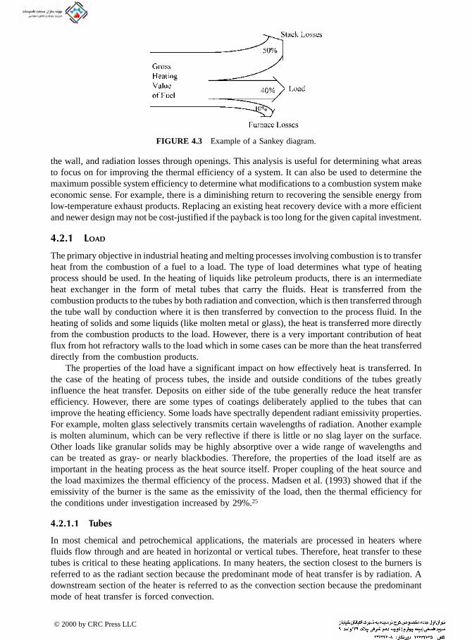
the wall, and radiation losses through openings. This analysis is useful for determining what areas to focus on for improving the thermal efficiency of a system. It can also be used to determine the maximum possible system efficiency to determine what modifications to a combustion system make economic sense. For example, there is a diminishing return to recovering the sensible energy from low-temperature exhaust products. Replacing an existing heat recovery device with a more efficient and newer design may not be cost-justified if the payback is too long for the given capital investment.
4.2.1 LOAD
The primary objective in industrial heating and melting processes involving combustion is to transfer heat from the combustion of a fuel to a load. The type of load determines what type of heating process should be used. In the heating of liquids like petroleum products, there is an intermediate heat exchanger in the form of metal tubes that carry the fluids. Heat is transferred from the combustion products to the tubes by both radiation and convection, which is then transferred through the tube wall by conduction where it is then transferred by convection to the process fluid. In the heating of solids and some liquids (like molten metal or glass), the heat is transferred more directly from the combustion products to the load. However, there is a very important contribution of heat flux from hot refractory walls to the load which in some cases can be more than the heat transferred directly from the combustion products.
The properties of the load have a significant impact on how effectively heat is transferred. In the case of the heating of process tubes, the inside and outside conditions of the tubes greatly influence the heat transfer. Deposits on either side of the tube generally reduce the heat transfer efficiency. However, there are some types of coatings deliberately applied to the tubes that can improve the heating efficiency. Some loads have spectrally dependent radiant emissivity properties. For example, molten glass selectively transmits certain wavelengths of radiation. Another example is molten aluminum, which can be very reflective if there is little or no slag layer on the surface. Other loads like granular solids may be highly absorptive over a wide range of wavelengths and can be treated as gray- or nearly blackbodies. Therefore, the properties of the load itself are as important in the heating process as the heat source itself. Proper coupling of the heat source and the load maximizes the thermal efficiency of the process. Madsen et al. (1993) showed that if the emissivity of the burner is the same as the emissivity of the load, then the thermal efficiency for the conditions under investigation increased by 29%.25
4.2.1.1 Tubes
In most chemical and petrochemical applications, the materials are processed in heaters where fluids flow through and are heated in horizontal or vertical tubes. Therefore, heat transfer to these tubes is critical to these heating applications. In many heaters, the section closest to the burners is referred to as the radiant section because the predominant mode of heat transfer is by radiation. A downstream section of the heater is referred to as the convection section because the predominant mode of heat transfer is forced convection.
FIGURE 4.3 Example of a Sankey diagram.
© 2000 by CRC Press LLC

The inside and outside conditions of the tubes in the radiant section greatly affect the heat transfer from the flame to the tubes. If the outside of the tubes becomes coated with a hydrocarbon, then
the radiant absorptivity of the tubes increases and the radiation from the flames to the tubes also increases. However, the heat transfer to the fluid inside the tubes may decrease as a result of a build-up on the outside of the tubes if the thermal conductivity of the coating is lower than that of the metal.
Biede et al. (1995) have shown that as slag from a pulverized coal combustor builds up on waterwall tubes, the heat transfer to the water in the tubes decreases and that the heat absorbed is a function of the slag composition.26 Harb et al. (1994) developed a model for the heat transfer through furnace wall deposits.27 The model calculates the fraction of particles that stick to the walls, the porosity and thermal conductivity of the deposit, and the fraction of liquid and crystalline phases in the deposit. The results showed that heat transfer to the wall rapidly decreased initially but then slowed asymptotically for longer times. The heat flux decreased by a factor of about 4 after only about 100 minutes. The model showed that the emittance of the deposit had only a relatively small effect on the heat transfer.
Hellander and Bryant (1993) described a ceramic coating that can be applied to the outside of process tubes to increase the heat transfer performance of the process heater.28 The coating has a high radiant emissivity (>0.85) and high thermal conductivity 580 Btu-in./ft2-hr-°F (84 W/m-K) so that it absorbs more radiation than an uncoated tube and conducts that energy readily through the thin (0.00175 to 0.00225 in., 0.0445 to 0.0572 mm) coating. The desired characteristics of such a coating include:
• Minimize surface reactions to prevent deposition and oxidation• Be non-stick to prevent the build-up of combustion products on the tubes• Prevent carbon and oxygen diffusion, which corrode the tubes• Be water-based and made of environmentally friendly materials• Cure quickly to minimize downtime for repairs• Be stable at temperatures of at least 1800°F (1300K)• Be thermally shock resistant
Efficiency improvements of 4% to 8% were reported for the coating.
4.2.1.2 Substrate
In many drying processes, moisture is removed from a substrate that is often traveling at high speeds. Common examples of these substrates include paper, carpets, plastics, metal sheets, and textiles. Radiant heating is often used in drying substrates, especially those with some type of surface coating where contact with a hot solid like a steam-heated cylinder or with high-velocity hot gases like in convection dryers can reduce the product quality.29 Examples are shown in Figures 1.20 and 4.4.
In radiant heating, to maximize efficiency, it is important to match the spectral output of the radiant source with the spectral radiant absorptivity of the load.30 Van der Drift et al. (1997) studied the effects of coatings on infrared burners on the efficiency of radiant heat transfer to a paper substrate and to a metal substrate coated with three different power paints (white, blue, and black).31
They showed that the thermal efficiency can be improved by as much as 10% by matching the radiant spectral output of the burner to the spectral absorptivity of the load. Both the paper and the paint powders had high absorptivities (nearly blackbody) above about 3 µm and very low absorp-tivities below about 3 µm.
4.2.1.3 Granular Solid
Many granular solids are heated in industrial furnaces. Common examples include cement and lime manufacturing. The heat transfer to granular solids has some unique challenges compared to other load materials. The surface of a granular solid often has a very high emissivity due to the many
© 2000 by CRC Press LLC
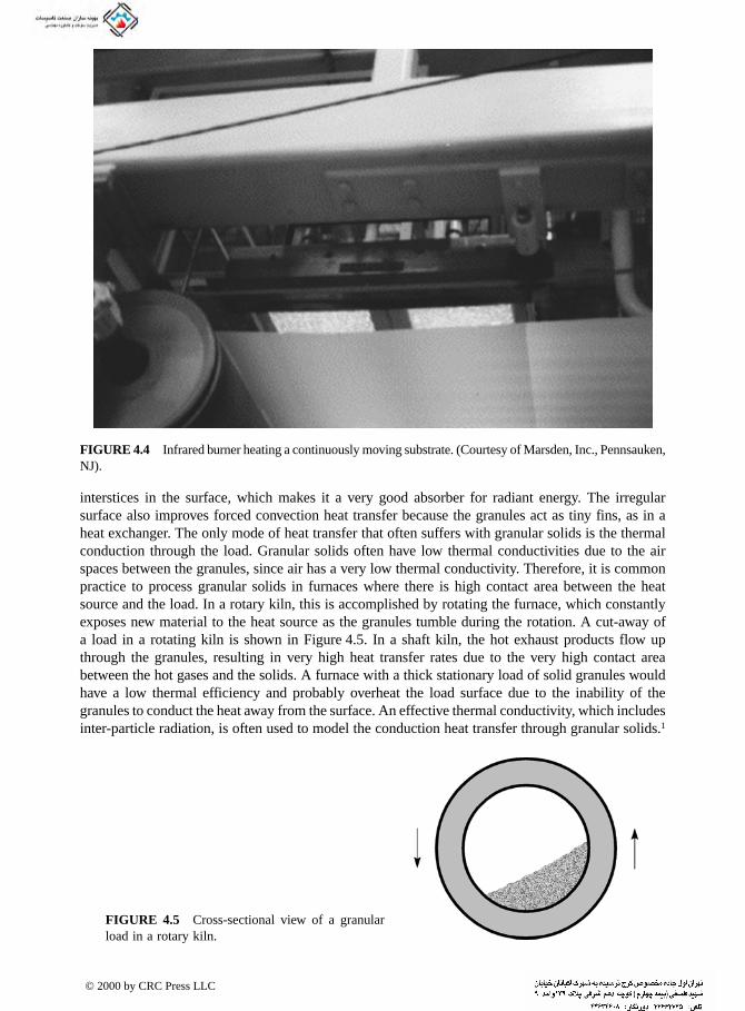
interstices in the surface, which makes it a very good absorber for radiant energy. The irregular surface also improves forced convection heat transfer because the granules act as tiny fins, as in a heat exchanger. The only mode of heat transfer that often suffers with granular solids is the thermal conduction through the load. Granular solids often have low thermal conductivities due to the air spaces between the granules, since air has a very low thermal conductivity. Therefore, it is common practice to process granular solids in furnaces where there is high contact area between the heat source and the load. In a rotary kiln, this is accomplished by rotating the furnace, which constantly exposes new material to the heat source as the granules tumble during the rotation. A cut-away of a load in a rotating kiln is shown in Figure 4.5. In a shaft kiln, the hot exhaust products flow up through the granules, resulting in very high heat transfer rates due to the very high contact area between the hot gases and the solids. A furnace with a thick stationary load of solid granules would have a low thermal efficiency and probably overheat the load surface due to the inability of the granules to conduct the heat away from the surface. An effective thermal conductivity, which includes inter-particle radiation, is often used to model the conduction heat transfer through granular solids.1
FIGURE 4.4 Infrared burner heating a continuously moving substrate. (Courtesy of Marsden, Inc., Pennsauken, NJ).
FIGURE 4.5 Cross-sectional view of a granular load in a rotary kiln.
© 2000 by CRC Press LLC

4.2.1.4 Molten Liquid
In a study by Ji and Baukal (1998), the nonluminous and luminous radiation from oxygen-enhanced flames were studied to determine the impact on melting glass.32 This was of particular interest because of the transparent characteristics of glass. The object of the study was to determine if nonluminous or luminous flames transfer more radiant heat to the molten glass and to determine which type of radiation penetrates deeper into the glass to minimize overheating of the glass surface. In glass melting, heat is transferred primarily by emission and absorption of flame radiation during the melting and much of the forming processes in the glass industry.33-36 The study by Ji and Baukal focused on the spectral radiation properties of natural gas flames that were enhanced with oxygen and on the absorption of flame radiation by molten glass. While there has been much theoretical research related to this subject,34,35,37 this was the first systematic experimental study on the spectral radiation properties of oxygen-enhanced/natural gas flames.
Because one of the most important heat transfer mechanisms in a glass furnace is absorption of the flame radiation by the glass melt, one must consider how flame radiation propagates through the glass melt over the entire spectral range. Several studies on high-temperature glass melt absorption spectra33,34,36,38 showed that the spectral absorption coefficient increases dramatically at about 2.7 µm. The glass melt essentially becomes opaque at longer wavelengths due to strong absorption from the O-H and Si-O bonds in silicate. This is a universal feature of molten glass. The spectral absorption at wavelengths shorter than 2.7 µm varies with the impurities and/or additives in the glass melt, the temperature, and the furnace atmosphere.33,36,38 For low iron (FeO) content molten glass without other impurities or additives, the spectral absorption at wavelengths shorter than 2.7 µm is relatively small and constant.34 The spectral absorption data of such low iron content glass melts in Reference 34 have been used for the case study in this work. Figure 4.6 shows the spectral absorption coefficient K of low iron content molten glass as reported in Reference 34. Also plotted in Figure 4.6 are the spectral radiation intensity of a flame with Ω = 1.0 and φ = 2.0, qf = 5 kW, and the intensity after the radiation propagates through 1 cm (0.4 in) of molten glass, respectively. It is evident from Figure 4.6 that only radiation at wavelengths λ < 2.7 µm has significant penetration into molten glass. Because glass is a poor heat conductor, the radiation energy at λ > 2.7 µm only heats the top
FIGURE 4.6 Interaction of flame radiation with high-temperature glass melt. (From B. Ji and C.E. Baukal, Proc. of 1998 International Gas Research Conference, Nov. 8-11, 1998, San Diego, CA, D. Dolenc, Ed., 5, 422-433, 1998.)
© 2000 by CRC Press LLC

surface of the glass, which can cause overheating that may reduce the glass quality. Therefore, only the penetrating (λ < 2.7 µm) radiation is the effective radiation for molten glass. In order to improve heat transfer efficiency and reduce fuel consumption in glass furnaces, it is important that the penetrating radiation intensity is maximized, rather than the total radiation intensity. To compare the penetrating radiation intensity among the various flames, the spectral radiation was numerically integrated for λ < 2.7 µm. The results are summarized in Table 3.5. For the penetrating radiation, the pure oxygen/natural gas flame produced 5 times more radiation than the air-fired flame, for the same fuel consumption and stoichiometry. Taking this into account, the fuel savings using oxygen enrichment is more pronounced for glass furnaces than the savings based only in terms of the total radiation. For oxygen/natural gas flames with different fuel equivalence ratios, a fuel-rich flame (φ = 2.00) apparently produced less total radiation than a stoichiometric flame (φ = 1.00), due to incom-plete combustion (see Table 3.5). However, the fuel-rich flame emits more penetrating radiation than a stoichiometric flame although not all the fuel was consumed.
4.2.1.5 Surface Conditions
Baukal and Gebhart (1997) studied the effects of the surface conditions on the heat transfer from impinging natural gas flames as shown in Figure 4.7.18 Different surface coatings were used to see how the radiation and thermochemical heat release were affected. The objective of this study was to determine the relative importance of thermal radiation and to determine how the thermochemical heat release is influenced by the surface properties of the target. The study investigated the heat transfer from oxygen-enhanced/natural gas flames (qf = 15 kW) impinging normal to a water-cooled metal disk (db = 135 mm) segmented into six concentric calorimetric rings as shown in Figure 4.8. The outer ring (#6) acted as a thermal guard to prevent lateral heat transfer into ring 5. A section view through a typical target cooling ring calorimeter is shown in Figure 4.9. A high-temperature, nickel-based, anti-seize lubricant was used between the layers to ensure good thermal contact. The back of the target, which contained the coolant inlet and outlet tubes, was fully insulated to thermally isolate each calorimeter. The steady-state cooled target technique39 was used to measure the heat flux to each calorimeter. These ring calorimeters were concentrically located around the stagnation point to determine the radial heat flux profiles. The inlet and outlet coolant temperatures to each calorimeter were measured with 4-wire resistance temperature detectors (RTDs). The total heat flux (q″i ), to each calorimeter ring i, was determined using:
(4.4)
FIGURE 4.7 Natural gas flame impinging on a water-cooled target. (From C.E. Baukal and B. Gebhart, Therm. Fluid Sci., 15, 323-335, 1997.)
′′=−( )
qm c t t
Ai
i p
i
i i˙
out in
© 2000 by CRC Press LLC

where •
mi is the cooling water mass flow rate to ring i, cp is the average specific heat of the cooling water, tout i
is the outlet temperature of the cooling water to ring i, tin i is the inlet temperature of the
cooling water to ring i, and Ai is the impingement surface area of ring i.
4.2.1.5.1 RadiationRadiation was not directly measured, but was inferred by comparing the total heat fluxes to surfaces with various emissivities. In many of the tests, the target surface was untreated. Both the brass and the stainless steel surfaces were relatively reflective in their natural state. The natural state of the copper was not as reflective as the brass or the stainless steel. The untreated brass and copper surfaces oxidized rapidly, after less than an hour of flame impingement testing. The stainless steel surfaces oxidized much more slowly. They were reflective even after several hours of testing. In one type of test, the target surface was highly polished. This was done to make the surface reflective to minimize its radiant absorptivity. In another type of test, the target surface was coated with a highly absorptive, high-temperature flat black paint, similar to lampblack. The typical emissivities
FIGURE 4.8 Plan view of target. (From C.E. Baukal and B. Gebhart, Therm. Fluid Sci., 15, 323-335, 1997.)
FIGURE 4.9 Section view through a typical target calorim-eter ring. (From C.E. Baukal and B. Gebhart, Therm. Fluid Sci., 15, 323-335, 1997.)
© 2000 by CRC Press LLC
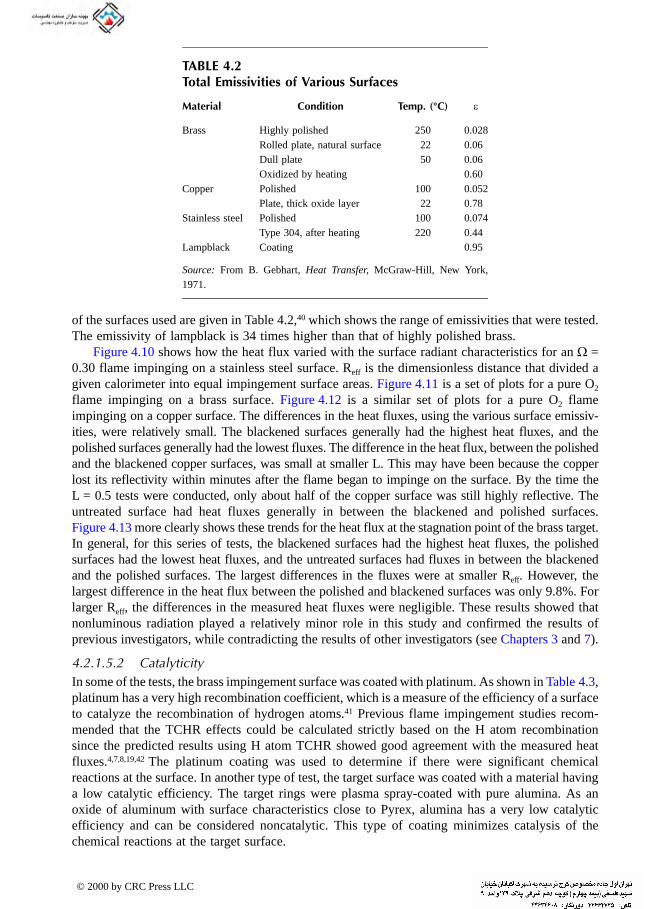
TABLE 4.2
of the surfaces used are given in Table 4.2,40 which shows the range of emissivities that were tested. The emissivity of lampblack is 34 times higher than that of highly polished brass.
Figure 4.10 shows how the heat flux varied with the surface radiant characteristics for an Ω = 0.30 flame impinging on a stainless steel surface. Reff is the dimensionless distance that divided a given calorimeter into equal impingement surface areas. Figure 4.11 is a set of plots for a pure O2
flame impinging on a brass surface. Figure 4.12 is a similar set of plots for a pure O2 flame impinging on a copper surface. The differences in the heat fluxes, using the various surface emissiv-ities, were relatively small. The blackened surfaces generally had the highest heat fluxes, and the polished surfaces generally had the lowest fluxes. The difference in the heat flux, between the polished and the blackened copper surfaces, was small at smaller L. This may have been because the copper lost its reflectivity within minutes after the flame began to impinge on the surface. By the time the L = 0.5 tests were conducted, only about half of the copper surface was still highly reflective. The untreated surface had heat fluxes generally in between the blackened and polished surfaces. Figure 4.13 more clearly shows these trends for the heat flux at the stagnation point of the brass target. In general, for this series of tests, the blackened surfaces had the highest heat fluxes, the polished surfaces had the lowest heat fluxes, and the untreated surfaces had fluxes in between the blackened and the polished surfaces. The largest differences in the fluxes were at smaller Reff. However, the largest difference in the heat flux between the polished and blackened surfaces was only 9.8%. For larger Reff, the differences in the measured heat fluxes were negligible. These results showed that nonluminous radiation played a relatively minor role in this study and confirmed the results of previous investigators, while contradicting the results of other investigators (see Chapters 3 and 7).
4.2.1.5.2 CatalyticityIn some of the tests, the brass impingement surface was coated with platinum. As shown in Table 4.3, platinum has a very high recombination coefficient, which is a measure of the efficiency of a surface to catalyze the recombination of hydrogen atoms.41 Previous flame impingement studies recom-mended that the TCHR effects could be calculated strictly based on the H atom recombination since the predicted results using H atom TCHR showed good agreement with the measured heat fluxes.4,7,8,19,42 The platinum coating was used to determine if there were significant chemical reactions at the surface. In another type of test, the target surface was coated with a material having a low catalytic efficiency. The target rings were plasma spray-coated with pure alumina. As an oxide of aluminum with surface characteristics close to Pyrex, alumina has a very low catalytic efficiency and can be considered noncatalytic. This type of coating minimizes catalysis of the chemical reactions at the target surface.
Total Emissivities of Various Surfaces
Material Condition Temp. (°C) ε
Brass Highly polished 250 0.028Rolled plate, natural surface 22 0.06Dull plate 50 0.06Oxidized by heating 0.60
Copper Polished 100 0.052Plate, thick oxide layer 22 0.78
Stainless steel Polished 100 0.074Type 304, after heating 220 0.44
Lampblack Coating 0.95
Source: From B. Gebhart, Heat Transfer, McGraw-Hill, New York, 1971.
© 2000 by CRC Press LLC
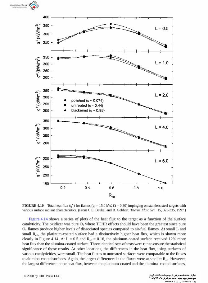
Figure 4.14 shows a series of plots of the heat flux to the target as a function of the surface catalyticity. The oxidizer was pure O2 where TCHR effects should have been the greatest since pure O2 flames produce higher levels of dissociated species compared to air/fuel flames. At small L and small Reff, the platinum-coated surface had a distinctively higher heat flux, which is shown more clearly in Figure 4.14. At L = 0.5 and Reff = 0.16, the platinum-coated surface received 12% more heat flux than the alumina-coated surface. Three identical sets of tests were run to ensure the statistical significance of those results. At other locations, the differences in the heat flux, using surfaces of various catalyticities, were small. The heat fluxes to untreated surfaces were comparable to the fluxes to alumina-coated surfaces. Again, the largest differences in the fluxes were at smaller Reff. However, the largest difference in the heat flux, between the platinum-coated and the alumina–coated surfaces,
FIGURE 4.10 Total heat flux (q″) for flames (qf = 15.0 kW, Ω = 0.30) impinging on stainless steel targets with various surface radiant characteristics. (From C.E. Baukal and B. Gebhart, Therm. Fluid Sci., 15, 323-335, 1997.)
© 2000 by CRC Press LLC

was only 12%. For L > 0.5, the difference in the heat flux between the platinum and alumina surfaces was negligible.
There are two important factors related to that study that determined the importance of TCHR. These include the temperature and the composition of the flame gases. As was shown in Chapter 2, these are related to each other and more dissociated species are normally produced in high Ωflames, compared to low Ω flames. It has also already been shown that TCHR is related to the amount of chemical energy contained in the combustion gases. Higher levels of dissociation increase the amount of chemical energy (hC) contained in the gases. This chemical energy is of two types. Some of the energy is contained in the form of unburned fuels like CO and H2. Some of the energy is also contained in the form of dissociated species like O, H, and OH. When the dissociated species
FIGURE 4.11 Total heat flux (q″) for O2 /natural gas flames (qf = 15.0 kW) impinging on brass targets with various surface radiant characteristics. (From C.E. Baukal and B. Gebhart, Therm. Fluid Sci., 15, 323-335, 1997.)
© 2000 by CRC Press LLC
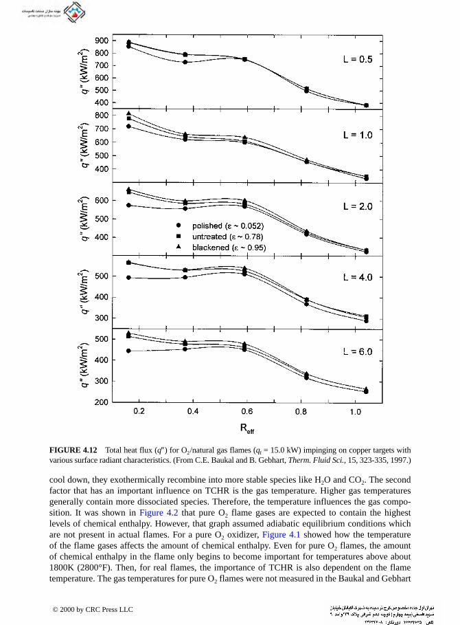
cool down, they exothermically recombine into more stable species like H2O and CO2. The second factor that has an important influence on TCHR is the gas temperature. Higher gas temperatures generally contain more dissociated species. Therefore, the temperature influences the gas compo-sition. It was shown in Figure 4.2 that pure O2 flame gases are expected to contain the highest levels of chemical enthalpy. However, that graph assumed adiabatic equilibrium conditions which are not present in actual flames. For a pure O2 oxidizer, Figure 4.1 showed how the temperature of the flame gases affects the amount of chemical enthalpy. Even for pure O2 flames, the amount of chemical enthalpy in the flame only begins to become important for temperatures above about 1800K (2800°F). Then, for real flames, the importance of TCHR is also dependent on the flame temperature. The gas temperatures for pure O2 flames were not measured in the Baukal and Gebhart
FIGURE 4.12 Total heat flux (q″) for O2 /natural gas flames (qf = 15.0 kW) impinging on copper targets with various surface radiant characteristics. (From C.E. Baukal and B. Gebhart, Therm. Fluid Sci., 15, 323-335, 1997.)
© 2000 by CRC Press LLC

study,18 but appear to have been well over 2400K (3900°F) based on the failure of the type L thermocouple at much lower oxidizer compositions. Although no quantitative conclusions could be made concerning TCHR, it appears there would have been substantial quantities of radical species in the impinging gases so that TCHR should have been an important mode of heat transfer for the Ω = 1.00 flames.
No method is known for directly measuring TCHR. In the Baukal and Gebhart study,18 one objective was to determine if catalytic TCHR was important. Three types of surfaces were tested: platinum-coated, untreated, and alumina-coated. If the catalyticity of the surface was important, then the heat fluxes to the platinum-coated surface should have been noticeably higher than the fluxes to the alumina-coated surface. The measurements showed that there was very little difference in the fluxes, except for small R and L. This confirmed the observations of Kilham and Purvis (1978), who studied O2 /CH4 and O2 /C3H8 flames impinging on flat refractory blocks.8 Both silicon carbide and platinum calorimeters were imbedded flush with the surface of the blocks. No differ-ences in the heat fluxes were detected using these two types of calorimeters. The results of the
FIGURE 4.13 Total heat flux (q″) for O2 /natural gas flames (qf = 15.0 kW) impinging on the stagnation point (Reff = 0.16) of brass targets with various surface radiant characteristics. (From C.E. Baukal and B. Gebhart, Therm. Fluid Sci., 15, 323-335, 1997.)
TABLE 4.3Recombination Coefficient of Various Surfaces for Hydrogen Atoms
Surface Ti V Cr Mn Fe Ni Cu Pd Pt Ag Au Al Pyrex
Recombination coefficient
0.10 0.15 0.16 0.20 0.17 0.18 0.19 0.20 0.25 0.13 0.10 0.001 0.00075
Source: From B.J. Wood and H. Wise, J. Chem. Phys., 29, 1416-1417, 1958.
© 2000 by CRC Press LLC

Baukal and Gebhart study also showed that a platinum-coated surface only enhanced the heat transfer at very close axial and radial target locations. Platinum is one of the most widely used catalysts in catalytic combustion.43 It is commonly used to oxidize hydrocarbons at much lower temperatures than is possible in normal flames. These lower temperatures significantly reduce pollutant emissions, especially NOx, which is exponentially dependent on the gas temperature. At close distances between the flame and the target, the combustion reactions may not have been fully completed. The platinum may have enhanced those reactions.
The differences in the heat flux, with and without the platinum coating, were relatively small. There are several possible explanations for this. The first is the low surface-area-to-volume ratio for platinum applied to a flat surface. Normally, catalysts are applied to high surface area substrates,
FIGURE 4.14 Total heat flux (q″) for O2 /natural gas flames (qf = 15.0 kW) impinging on brass targets with various surface catalyticities. (From C.E. Baukal and B. Gebhart, Therm. Fluid Sci., 15, 323-335, 1997.)
© 2000 by CRC Press LLC

such as a honeycomb structure. A coating on a flat surface, as used by Baukal and Gebhart, has a very low surface-area-to-volume ratio compared to common catalyst supports. Higher surface areas
enhance the effect of the catalyst.44 Deterioration of the catalyst is another effect that may have reduced the catalyticity of the platinum.45 After only a few test runs, the platinum surface conditions visibly changed. The initially reflective surface obtained a darker, less reflective appearance. This change in the surface may have indicated a reduction in the catalyst effectiveness. A third possible explanation is that catalytic TCHR was not an important effect for the conditions studied. It is well known that one must compensate for chemical recombination when using platinum thermocouples to measure gas temperatures in flames.46 This is usually done by coating the thermocouple with a material having a low catalyticity, such as silica. Leah and Carpenter (1953) showed how uncoated platinum thermocouples overpredict the temperature, compared to silica-coated thermocouples.47
However, in the Baukal and Gebhart study, no significant differences were observed using targets with either high or low catalyticity. This may be explained in several ways. Equilibrium TCHR may be a much more dominant mechanism. The much cooler gases in the stagnation region may cause the dissociated species to react before they contact the surface. The reaction times may be small compared to the diffusion times to the surface. Therefore, the concentration of dissociated species may have been very small by the time the gases reached the target surface. A second effect may have been the fluid dynamics. Many of the flame gases may never have contacted the surface, due to the boundary layer. A third explanation may be that the gas residence time, compared to the time for the species to diffuse to the surface, may have been too short. There may not have been enough time for the gases to react at the surface before being carried away by the flow. In any case, catalytic TCHR did not appear to be a significant mechanism for the flame impingement conditions studied there. Because mixed TCHR is a combination of equilibrium and catalytic TCHRs, one might also conclude that mixed TCHR was not an important mechanism. It has been shown that the heat transfer correlations may predict nearly identical heat fluxes for either equi-librium or catalytic TCHR, depending on the test conditions.17
Figure 4.15 shows a comparison of the effects of both the radiative and catalytic surface properties. The platinum-coated surface clearly had the highest heat flux. There was little difference in the heat flux to the target with the other surface conditions.
4.2.2 WALL LOSSES
No industrial combustor is perfectly insulated, which means that heat will flow from the inside of the combustor to the outside environment by thermal conduction. An example of calculating conduction losses through a refractory wall was given in Chapter 3. Wall losses are important for many reasons. High wall losses can significantly reduce the thermal efficiency of a process. High outside combustor temperatures due to high wall losses can be a safety hazard to personnel operating the equipment. Hotspots on the outside wall can be an indicator of a problem where refractory may have become damaged or thinned due to the process, or flames may be impinging undesirably on the wall, which may be a problem caused by the burners or improper operating conditions. The type and thickness of refractory used in a combustor depends on many factors, especially economics. Again, there is a diminishing return to increasing the thickness of the refractory, which may only give a marginal reduction in the heat loss through the wall and is typically a relatively small fraction of the overall heat losses in a system. Reed (1986) has given a good discussion of calculating wall losses and included tables and graphs, using real materials used in industrial combustors, for making these calculations more quickly.48
Wall losses are due to both radiation and convection. The skin temperature of the outside furnace wall, usually a metal, is at a temperature higher than the ambient surroundings, causing energy to radiate from the wall to the ambient. For analysis purposes, the ambient is considered to be a large enclosure at a constant temperature so that the view factor from the wall to the
© 2000 by CRC Press LLC

surroundings can be considered to be one. Then, the radiant losses from the outside combustor wall to the surroundings can be simply calculated using:
(4.5)
where εw and Tw are the emissivity and absolute temperature of the wall, respectively, A is the area of the wall, and T× is the absolute temperature of the ambient.
There are two types of convection that can be important in calculating wall losses, depending on the ambient conditions. Forced convection is only significant if there is gas flow over the surface of the outside combustor wall. This can be the case for combustors located outside where the wind may be a factor. The average forced convection heat transfer coefficient for flow parallel to an isothermal plate can be calculated using:49
(4.6)
where =–
hl/k, Rel = ρvl/µ is the Reynolds number calculated with the length l in the direction of the flow and Pr = cpµ/k for the air flowing over the plate.
Example 4.1
Given: Air at 81°F flowing at 20 miles/hr parallel to the outer wall (20 ft in the direction of flow and 10 ft high) of a furnace where the wall temperature is 150°F.
Find: Heat lost from the wall by forced convection.
FIGURE 4.15 Total heat flux (q″) for O2 /natural gas flames (qf = 15.0 kW) at a fixed axial position (L = 0.5), for brass targets with various surface treatments. (From C.E. Baukal and B. Gebhart, Therm. Fluid Sci.,15, 323-335, 1997.)
qw,rad w w4 4= −( )∞ε σA T T
Nu = 0 037 4 5 1 3. Re Prl
Nu
© 2000 by CRC Press LLC

Solution: Determine gas properties for air at 81°F (see Table F.1a):
ρ = 0.0725 lb/ft3, k = 0.0152 Btu/ft-hr-°F, µ = 0.0447 lb/ft-sec, Pr = 0.707
Calculate Re and then Nu:
v = 20 miles/hr = 29 ft/sec,
Re = (0.0725 lb/ft3)(29 ft/s)(20 ft)/(1.24 × 10–5 lb/ft-sec) = 3.39 × 10⁶,
= 0.037(3.39 × 10⁶)4/5 (0.707)1/3 = 5524
Calculate h = Nu k/l = (5524)(0.0152 Btu/ft-hr-°F)/(20 ft) = 4.20 Btu/ft2-hr-°F
Solve for heat loss: q = h A (tw – t×)
= (4.20 Btu/hr-ft2-°F)(20 ft × 10 ft)(150°F – 81°F)
= 58,000 Btu/hr
For the relatively narrow temperature range given in this problem, there is very little variation in the properties with temperature. It may be desirable to compute the properties at the film temperature defined as:
(4.7)
Natural convection occurs because the furnace wall is at a higher temperature than the sur-roundings, which causes the air next to the wall to heat up and then rise due to buoyancy. Convective heat transfer coefficients for the free convection of air from a surface can range from 1 to 5 Btu/hr-ft2-°F (6 to 30 W/m2-K).50 The actual value depends on the geometry and temperature difference between the wall and the ambient. Holman (1981) has given some simplified equations for natural convection from various surfaces to ambient air.51 For laminar (104 < Grf Prf < 109) natural convection from vertical surfaces to air:
(4.8)
where tw is the wall temperature, t× is the air temperature, and l is the vertical length of the wall. For turbulent (Grf Prf > 109) natural convection from a vertical surface to air:
(4.9)
For laminar (104 < Grf Prf < 109) natural convection from a heated flat plat facing upward to air:
(4.10)
For turbulent (Grf Prf > 109) natural convection from a heated flat plat facing upward to air:
(4.11)
where the Grashoff number is calculated from:
(4.12)
Nu
tt t
fw= − ∞
2
ht t
lw= −⎛
⎝⎞⎠
∞1 421 4
.
h t tw= −( )∞0 951 3
.
ht t
lw= −⎛
⎝⎞⎠
∞1 321 4
.
h t tw= −( )∞1 431 3
.
Grg t t lw=
−( )∞βν
3
2
© 2000 by CRC Press LLC

where g is the gravity constant, β∼
is the volume coefficient of expansion (= 1/T for an ideal gas), and ν is the kinematic viscosity. Both the Grashoff and Prandtl numbers are calculated at the film
temperature tf.
4.2.3 OPENINGS
Energy can be lost by openings in the furnace by one of two mechanisms. Heat can be radiated out of the hot furnace to the cooler surroundings, or gases can travel through openings in the furnace (ambient air can infiltrate into the furnace or hot gases can exit through openings). Both are briefly discussed here.
4.2.3.1 Radiation
Most industrial combustion chambers can be considered to be a blackbody when calculating the radiant heat loss from relatively small openings in the furnace. The view factor from a small opening to the ambient environment can be considered to be one. Then, the radiant heat loss from a furnace opening to the surroundings can be simply calculated using:
(4.13)
where A is the area of the opening.
Example 4.2
Given: Average furnace interior temperature = 1500°F; ambient temperature = 70°F; opening of 4 in. × 10 in.
Find: Heat lost from the opening by radiation.
Solution: qopening,rad = (0.1714 × 10⁻⁸ Btu/hr-ft2-(R4)(4/12 ft × 10/12 ft)(19604 – 5304)°R4
= 14,000 Btu/hr
Radiant losses through furnace openings can present several problems. They obviously reduce the efficiency of the process. They can present a hazard to personnel working around the furnace. They can also damage surrounding equipment, particularly electronics, which are not capable of handling the radiant heat load and higher temperatures.
Some furnaces are equipped with sight or view ports for operators to look into the furnace to view the operation. Although some view ports have no window and are just an opening in the furnace, accepted safety practice is to have some type of glass over the opening to protect the operators from hot gases exiting the furnaces through those ports. These windows are typically made of quartz, which can handle high temperatures. A good view port design should have a movable shutter between the inside of the furnace and the glass to minimize heat losses from the view port and to protect the glass from the high temperatures and any particles in the furnace atmosphere that might accumulate on the glass and obscure the view. The heat loss through the glass is less than through an uncovered opening because the glass only transmits part of the radiation hitting it. Glass selectively transmits radiant energy as a function of wavelength, so the actual amount of radiation transmitted through the glass is dependent on its spectral characteristics. To simply calculations, an average transmissivity is usually used.
4.2.3.2 Gas Flow Through Openings
The second major type of heat loss through a furnace opening is by gas flow through openings in the furnace. Depending on the furnace pressure conditions at the opening, cold air from outside
q A Topening,rad w= −( )∞σ 4 4T
© 2000 by CRC Press LLC

the furnace may be drawn inside, or hot gases inside the furnace may exit through the openings. Many industrial combustion processes are operated at negative furnace pressures to prevent any of
the gases in the furnace from leaking into the environment. This protects the operators and equipment in the surrounding area from being overheated. If there are toxic chemicals in the process, negative furnace pressures also protect them from toxic gases leaking into the environment. For example, waste incinerators are operated at negative furnace pressures to prevent any of the waste gases from going into the environment until they have been fully incinerated and treated in downstream scrubbing equipment. A large potential source of air infiltration for batch heating processes occurs when charge doors are opened to add new charge materials or to remove finished products. Another potentially large source for air infiltration are the openings used to transport materials into and out of continuous furnaces where there must be some type of gap for the materials to enter the furnace. When cold air leaks into a furnace, it absorbs sensible energy from the process. This reduces the thermal efficiency of the process. However, it is often possible to adjust the combustion process to account for this air leakage by reducing the amount of combustion air flow to the burners. It is still preferable to minimize air infiltration as it is by nature uncontrolled, which makes it more difficult to control the overall combustion system. Assuming that any air leaking into a furnace does not participate in the combustion process but merely absorbs sensible energy, the heat loss can be calculated using:
(4.14)
where •
mair is the mass flow rate of air, cp is the average specific heat of the air, and texhaust is the temperature of the air when it exits the flue.
Example 4.3
Given: Ambient air (70°F) is infiltrating into a furnace at a rate of 100 scfh; the exhaust gas temperature is 1800°F.
Find Heat lost due to air infiltration.
Solution:•
mair = (10 ft3/hr)(0.075 lb/ft3 at 70°F) = 0.75 lb/hr
qair infiltration = (0.75 lb/hr)(0.24 Btu/lb-°F)(1800°F – 70°F) = 311 Btu/hr
In this example, the heat loss due to air infiltration is very small. This mechanism only becomes significant for large volumes of air infiltration. Note that although the flow rate of infiltrating air is almost impossible to measure directly, it is fairly simple to calculate. It requires an accurate measure of the fuel and combustion air flow rates into the furnace and of the O2 content in the exhaust gas products. The composition of the combustion products is estimated, without air infiltration, using the principles discussed in Chapter 2. Then, the measured O2 in the exhaust is compared against the calculated value, which should be lower. The difference is then attributed to air infiltration. Simple chemical and mass balances are then used to estimate how much air infiltrated into the process.
The second way heat can be lost from gas flow through a furnace opening is by hot gases flowing out of the opening. Some industrial combustion processes are operated at slightly positive furnace pressures to prevent air from infiltrating into the process. One example is heat treating systems that often require very low levels of oxygen in the furnace atmosphere to produce high-quality parts. Uncontrolled air leakage into that type of process would reduce the product yields. Then, for this type of process, it is preferred to have a slight flow of gases exiting the furnace. Hot gases exiting a furnace constitute a different type of heat loss that is often more difficult to estimate. If there were no openings in the furnace except for the exhaust stack, these gases would eventually exit the furnace anyway. By leaking out before reaching the designed exit (exhaust stack), these gases do not have an opportunity to release more of their heat inside the furnace. This means that
q m c t tair pair infiltration exhaust= −( )∞˙
© 2000 by CRC Press LLC

they may also leak out at a higher temperature than if they exited out of the stack. Determining the temperature and flow rate of the gases exiting out openings other than the flue and estimating
how much energy they would have released if they had remained in the furnace longer are somewhat difficult to determine. This calculation requires fairly specific knowledge about a specific process and is beyond the scope of this book.
4.2.4 MATERIAL TRANSPORT
Another potential heat loss in a combustion system is the transport system used for putting materials into and taking materials out of the combustor. Some examples will serve to illustrate this type of loss. In a walking-beam steel reheat furnace, rectangular steel bars are “walked” through the furnace on beams under the bars. These beams lift the bars and carry them forward an incremental distance at discrete time intervals depending on the specific process. The beams may be water-cooled steel or may be made of a hard refractory to protect them from the heat. The water-cooled beams will obviously remove more heat from the process than refractory beams, but they will also last longer. Another example of material transport losses is in a belt furnace where parts are loaded onto a metal mesh belt so they can be carried through the furnace. If the belt remained mostly inside the furnace, except for a small section at the entrance where the parts are loaded, then the heat losses would be minimal. However, most of these heat-treating furnaces have an internal cooling zone in the furnace that is an integral part of the heat-treating process in order to get the desired metal properties. In that case, the metal mesh belt carries a significant amount of energy out of the process because the cooling zone typically blows cool gases onto the parts being heat-treated and through the belt, which cools the belt and carries away heat.
A different type of heat loss involving the material transport system is when the product being heated is being circulated out of the furnace during a portion of the cycle. An example is in a side-well aluminum reverberatory furnace (see Chapter 11) where the molten aluminum is circulated outside the combustion chamber where cold scrap material can be added into the circulating metal bath. In that case, there will be radiation and natural convection losses from the molten aluminum exposed to the ambient environment.
REFERENCES
1. H.C. Meisingset, J.G. Balchen, and R. Fernandez, Mathematical modelling of a rotary hearth calciner, Light Metals 1996, W. Hale, Ed., The Minerals, Metals & Materials Society, Warren, PA, 1996, 491-497.
2. R. Conolly and R.M. Davies, A study of convective heat transfer from flames, Int. J. Heat Mass Trans., 15, 2155-2172, 1972.
3. M.E. Horsley, M.R.I. Purvis, and A.S. Tariq, Convective heat transfer from laminar and turbulent premixed flames, Heat Transfer 1982, U. Grigull, E. Hahne, K. Stephan, and J. Straub, Eds., Hemi-sphere, Washington, D.C., 3, 409-415, 1982.
4. J.K. Kilham and M.R.I. Purvis, Heat Transfer From Hydrocarbon-Oxygen Flames, Comb. Flame, 16, 47-54, 1971.
5. R. Viskanta, Heat transfer to impinging isothermal gas and flame jets, Exper. Therm. Fluid Sci., 6, 111-134, 1993.
6. J.A. Fay and F.R. Riddell, Theory of stagnation point heat transfer in dissociated air, J. Aero. Sci., 25, 73-85, 1958.
7. W.H. Giedt, L.L. Cobb and E.J. Russ, Effect of Hydrogen Recombination on Turbulent Flow Heat Transfer, ASME Paper 60-WA-256, New York, 1960.
8. J.K. Kilham and M.R.I. Purvis, Heat transfer from normally impinging flames, Comb. Sci. Tech., 18, 81-90, 1978.
9. R.A. Cookson and J.K. Kilham, Energy transfer from hydrogen-air flames, Ninth Symposium (Inter-national) on Combustion, Academic Press, New York, 1963, 257-263.
© 2000 by CRC Press LLC

10. J.K. Kilham and P.G. Dunham, Energy transfer from carbon monoxide flames, Eleventh Symposium (International) on Combustion, The Comb. Inst., Pittsburgh, PA, 1967, 899-905.
11. A. Ivernel and P. Vernotte, Etude expérimentale de l’amélioration des transferts convectis dans les
fours par suroxygénation du comburant, Rev. Gén. Therm., Fr., 210-211, 375-391, 1979.12. J.M. Beér and N.A. Chigier, Impinging jet flames, Comb. Flame, 12, 575-586, 1968.13. A. Milson and N.A. Chigier, Studies of methane-air flames impinging on a cold plate, Comb. Flame,
21, 295-305, 1973.14. D.E. Rosner, Convective Heat Transfer with Chemical Reaction, Aeron. Res. Lab. Rept. ARL 99,
Part 1, AD269816, 1961.15. R.A. Cookson, An Investigation of Heat Transfer from Flames, Ph.D. thesis, The University of Leeds,
Leeds, U.K., 1960.16. C.E., Baukal, L.K. Farmer, B. Gebhart, and I. Chan, Heat transfer mechanisms in flame impingement
heating, Proceedings of the 1995 Int’l Gas Research Conference, D.A. Dolenc, Ed., Gov’t Institutes, Inc., Rockville, MD, 2, 2277-2287, 1996.
17. C.E. Baukal and B. Gebhart, A review of semi-analytic solutions for flame impingement heat transfer, Int. J. Heat Mass Trans., 39(14), 2989-3002, 1996.
18. C.E. Baukal and B. Gebhart, Surface condition effects on flame impingement heat transfer, Therm. Fluid Sci., 15, 323-335, 1997.
19. S. Nawaz, Heat Transfer from Oxygen Enriched Methane Flames, Ph.D. thesis, The University of Leeds, Leeds, U.K., 1973.
20. S. Gordon and B.J. McBride, Computer Program for Calculation of Complex Chemical Equilibrium Compositions, Rocket Performance, Incident and Reflected Shocks, and Chapman-Jouget Detonations, NASA Report SP-273, Washington, D.C., 1971.
21. S. Gordon, B.J. McBride, and F.J. Zeleznik, Computer Program for Calculation of Complex Chemical Equilibrium Compositions and Applications. Supplement I. Transport Properties, NASA Technical Memorandum 86885, Washington, D.C., 1984.
22. E. Buhr, G. Haupt, and H. Kremer, Heat transfer from impinging turbulent jet flames to plane surfaces, Combustion Institute European Symposium 1973, F.J. Weinberg, Ed., Academic Press, New York, 1973, 607-612.
23. J.K. Kilham and M.R.I. Purvis, Heat transfer from normally impinging flames, Comb. Sci. Tech., 18, 81-90, 1978.
24. W.A. Hardy and J.W. Linnett, Mechanisms of atom recombination on surfaces, Eleventh Symposium (International) on Combustion, The Combustion Institute, Pittsburgh, PA, 1967, 167-179.
25. O.H. Madsen, M. Andersen, R.E. Peck, and M.R. Kulkarni, Infrared flux matching for improved radiant heating, Proc. of 1992 International Gas Research Conf., H.A. Thompson, Ed., Govt. Institutes, Rockville, MD, 1993, 2025-2034.
26. O. Biede, J.S. Lund, R. Thiemke, O. Rathmann, and L. Wolff, Measured heat absorption in a test furnace for various coal types, Proceedings of the 3rd European Conf. on Industrial Furnaces and Boilers, Lisbon, Portugal, 18-21 April, 1995.
27. J.N. Harb, P.N. Slater and G.H. Richards, A mathematical model for the build-up of furnace wall deposits, Proceedings of the Conf. on the Impact of Ash Deposition on Coal-Fired Plants, Solihull, U.K., June 1993, Taylor & Francis, 1994, 637-644.
28. J.C. Hellander and G.B. Bryant, Use ceramic coatings to improve efficiency of gas-fired furnaces, Hydrocarbon Processing, 72(10), 59-60, 1993.
29. P. Colette, Surface of coated grades enhanced by high intensity infrared drying, Pulp and Paper, 64, 89-95, 1990.
30. O.H. Madsen, M. Andersen, R.E. Peck, and M.R. Kulkarni, Infrared flux matching for improved radiant heating, Proc. of 1992 International Gas Research Conf., Gas Research Institute, 16-19 November 1992, Orlando, FL, Gov’t Institutes Inc., Rockville, MD, 5, 74-83, 1992.
31. A. van der Drift, N.B.K. Rasmussen, and K. Jorgensen, Improved efficiency drying using selective emittance radiant burners, Applied Therm. Engrg., 1(8-10), 911-920, 1997.
32. B. Ji and C.E. Baukal, Spectral radiation properties of oxygen-enhanced/natural gas flames, Proceed-ings of 1998 International Gas Research Conference, Dan Dolenc, Ed., 8-11 November 1998, San Diego, CA, 5, 422-433, 1998.
© 2000 by CRC Press LLC

33. H. Franz, Infrared absorption of molten soda-lime-silica glasses containing transition metal oxides, Int. Congr. Glass, Sci. Tech. Comm., 9(1), 243-260, 1971.
34. J.I. Berg, Near infrared absorption coefficient of molten glass by emission spectroscopy, Int. J. of
Thermophysics, 2(4), 381-394, 1981.35. F. Ammouri, C. Champinot, W. Bechara, E. Djadvan, M. Till, and B. Marie, Influence of oxy-firing
on radiation transfer to the glass melt in an industrial furnace: importance of spectral radiation model, Glastech. Ber. Glass Sci. Tech., 70(7), 201-206, 1997.
36. J. Endrys, F. Geotti-Bianchini, and L. De Riu, Study of the high-temperature spectral behavior of container glass. Glastech. Ber. Glass Sci. Tech., 70(5), 126-136, 1997.
37. G.M. Faeth, J.P. Gore, S.G. Chuech, and S.-M. Jeng, Radiation from turbulent diffusion flames, Annu. Rev. of Fluid Mech. & Heat Transfer, 2, 1-38, 1989.
38. D. Banner and S. Klarsfeld, High temperature infrared spectra of silicate melts, Phys. Non-cryst. Solids, L.D. Pye, W.C. La Course, H.J. Stevens, Eds., London, 1992, 371-375.
39. ASTM, Standard Method for Measuring Heat Flux Using a Water-Cooled Calorimeter, American Society of Testing and Materials Standard E422, Philadelphia, PA, 1983.
40. B. Gebhart, 1971, Heat Transfer, McGraw-Hill, New York, 1971.41. B.J. Wood, and H. Wise, Diffusion and heterogeneous reaction. II. Catalytic activity of solids for
hydrogen-atom recombination, J. Chem. Phys., 29, 1416-1417, 1958.42. L.W. Woodruff, and W.H. Giedt, Heat transfer measurements from a partially dissociated gas with
high Lewis number, J. Heat Trans., 88, 415-420, 1966.43. H. Arai, and M. Machida, Recent progress in high-temperature catalytic combustion, Catalysis Today,
10, 81-95, 1991.44. H. Arai, T. Yamada, K. Eguchi, and T. Seiyama, Catalytic combustion of methane over various
Perovskite-type oxides, Applied Catalysis, 26, 265-276, 1986.45. R.L. Burwell, Synthesis gas formation by direct oxidation of methane over Pt monoliths, Chemtracts-
Inorganic Chemistry, 5, 100-105, 1993.46. R.M. Fristrom, Flame Structure and Processes, Oxford Univ. Press, New York, 1995.47. A.S. Leah, and N. Carpenter, The estimation of atomic oxygen in open flames and the measurement
of temperature, in Fourth Symposium (International) on Combustion, B. Lewis, H.C. Hottel, and A.J. Nerad, Eds., Williams and Wilkins Co., Baltimore, MD, 1953, 274-285.
48. R.J. Reed, North American Combustion Handbook. Volume I: Combustion, Fuels, Stoichiometry, Heat Transfer, Fluid Flow, 3rd edition, North Amer. Mfg. Co., Cleveland, OH, 1986.
49. R.H. Pletcher, External flow forced convection, in Handbook of Single-Phase Convective Heat Trans-fer, S. Kakaç, R.K. Shah, and W. Aung, Eds., Wiley, New York, 1987.
50. F. Kreith and M.S. Bohn, Principles of Heat Transfer, 4th edition, Harper & Row, New York, 1986.51. J.P. Holman, Heat Transfer, 5th edition, McGraw-Hill, New York, 1981.
© 2000 by CRC Press LLC

0-8493-7686-6/97/$0.00+$.50© 1997 by CRC Press LLC
5 Computer Modeling
5.1 COMBUSTION MODELING
There are many reasons to model a combustion system. The most obvious is to gain insight intoa particular configuration in order to optimize it. Optimization means different things to differentpeople. It may mean maximizing thermal efficiency, minimizing pollutant emissions, maximizingthroughput, minimizing operating costs, or some combination of these. Another reason to modelis in the development of new technologies. New geometries can be tested relatively quicklycompared to building an entire combustion system. Ideally, modeling is done in conjunction withexperimentation to validate a particular new design. Doing modeling first can save considerablyon prototype development time and costs by eliminating particular designs without having toactually test them. However, in most cases, it is not possible to completely eliminate prototypetesting because of the uncertainty and limitations of combustion modeling, especially when it comesto new configurations that may never have been tried before. Another reason for modeling is toaid in scaling systems to either larger or smaller throughputs. Simple velocity or residence timescaling laws often do not apply to complicated combustion problems.1 Modeling can be used forpredictive purposes to test different scenarios that may be too risky or expensive to try in an existingoperational industrial combustion system. For example, a glass producer may want to evaluate theimpact of replacing an existing air preheat system with pure oxygen. Another reason to do com-bustion modeling is to help determine the location for instrumentation. For example, models canbe used to help decide where to locate thermocouples in a furnace wall at potential hot spots inorder to prevent refractory damage. Although experiments are normally used to validate modelingresults, the opposite may also be true. In industrial combustion systems, large-scale probes may benecessary due to water-cooling requirements for survivability. These large probes can cause sig-nificant disturbances in the process, which can be simulated with models. The model results canthen be used to determine the relevance of experimental measurements. Models can also be usedto simulate potentially dangerous conditions to assess the consequences in order to design theproper safety equipment and procedures. A more recent use of computer modeling is for controlof processes where the models are used to predict the results under the given conditions and thenadjust the operating parameters to produce the desired results. This includes the use of artificialintelligence, where the control system has a large database of past operating conditions and theassociated results so that the system can then predict and adjust itself to meet new operatingconditions. Examples include making adjustments as equipment ages and deteriorates as well asfor new materials being processed. In the past, these adjustments would have been based on theknowledge and experience of the operators and were often trial-and-error. Newer control systemspromise more sophisticated and systematic evaluation of the given operating conditions and desiredresults.
One of the risks in computer modeling is that too much faith may be placed in the results. Sometend to believe anything generated by a computer. However, if the computer models have not beenproperly validated, then the results may be highly suspect. For the foreseeable future, it is likely thatmodels will continue to use various approximations (e.g., turbulence) in order to get solutions in areasonable amount of time. Therefore, the user must exercise good judgment and not try to overextendthe results beyond what is warranted. For example, in many cases, models are very useful in predictingpollutant emission trends but are often very inaccurate in predicting the actual emissions. Knowledgeof the model’s capabilities helps one understand which results are more reliable and which ones are
© 2000 by CRC Press LLC

less reliable. The bulk fluid flow and heat transfer in a combustion system can usually be predictedwith a high degree of accuracy, while the small-scale turbulence and trace species predictions maybe less reliable. Therefore, it is recommended that computer modeling of combustion systems onlybe done by those who have been properly trained in that area.
Patankar and Spalding (1974) noted some of the important aspects of the problem statementfor industrial combustion modeling problems:2
• Geometry of the combustion chamber• Fuel and air input conditions• Thermal boundary conditions• Thermodynamic, transport, radiative, and chemical-kinetic properties, and the desired
outputs of models• Velocity, temperature, composition, etc. throughout the chamber• Heat flux and temperature at the wall
A number of books have been written on the subject of modeling combustion processes.However, very few have specifically concerned large-scale industrial combustion systems. Khalil(1982) presented modeling results for six large-scale industrial furnaces that had published exper-imental data for comparison.3 These six studies had burners with and without quarls (burner tiles);methane, natural gas, and propane fuels; firing rates ranging from 0.74 to 13 MW (2.5 to 44 × 106
Btu/hr); furnace lengths ranging from 4.5 to 11 m (15 to 36 ft); and swirl numbers ranging from0 to 5.0. The modeling results using the k-ε turbulence model were in good agreement with thepublished experimental data. Oran and Boris (1991) have edited a large book on combustionmodeling.4 Part 1 of the book concerns modeling the chemistry of combustion; Part 2 containsinformation on flames and flame structure; Part 3 is on high-speed reacting flows; and Part 4 ishumorously entitled “(Even More) Complex Combustion Systems” and has chapters on liquid andsolid fuel combustion, as well as on pulse combustion. The book is more theoretical in nature andis intended for aerospace combustion. However, it does have some useful information pertinent toindustrial combustion, which is referred to later in this chapter. A book edited by Larrouturou(1991) looks at the modeling of some fundamental processes in combustion science, but does notspecifically consider large-scale industrial flames.5 The papers have significant discussions of flamechemistry and fluid dynamics, but very little on heat transfer from the flames. Chung (1993) hasedited a book that contains chapters on the various techniques used to model combustion processes,but without any specific applications to industrial combustion problems.6 In a handbook on fluiddynamics, Lilley (1998) has a brief treatment of combustion modeling with only very brief discus-sions of industrial applications.7 Many papers have also been written on the subject of modelingthe heat transfer in combustion systems, which are discussed here.
5.2 MODELING APPROACHES
A complete combustion system may be extremely complex and can include a wide range of physicalprocesses that are often highly interactive and interdependent. A given combustion system may include:
• Turbulent fluid dynamics in the flame with laminar fluid dynamics in the bulk of thecombustor
• Multidimensional flows, which could include swirl• Multiple phases that could include gases, liquids, and solids, depending on the fuel
composition• Very high temperature, velocity, and species gradients in the flame region with much
lower gradients in the bulk of the combustor
© 2000 by CRC Press LLC

• Large material property variations caused by the wide range of temperatures, species,and solids present in the system
• Multiple modes of heat transfer, especially radiation that is highly nonlinear and mayinclude wavelength dependence
• Complex chemistry involving numerous reactions and many species, most of which arein trace amounts
• Porous media• Catalytic chemical reactions in some limited applications• Complex, nonsymmetrical furnace geometries• Multiple flame zones produced by burners that may be operated at different conditions
and whose flames interact with each other• A heat load that may be moving and interacting with the combustion space above it in
a nonlinear manner• A heat load that may produce volatile species during the heating process• A heat load whose properties may vary greatly with temperature, physical state, and even
wavelength for radiation• A transient heating and melting process that may include discrete material additions and
withdrawals
There are many challenges caused by this complexity, including inadequate physics to properlymodel the problem, large numbers of grid points requiring large amounts of computer memory,and long computation times. The simulation results may be difficult to validate as many of theexperimental measurements are difficult, time-consuming, and costly to make in industrial com-bustors. Therefore, in most combustion simulations, simplifying assumptions must be made to getcost-effective solutions in the amount of time available for a given problem. The actual simplifi-cations depend on many factors, including the level of accuracy required, the available amount ofcomputing power, the skill and knowledge of the modeler, the experience with the given systembeing simulated, and the time available to get a solution. These simplifying approaches are brieflydiscussed here. More detailed information on each aspect of the modeling is given later in thischapter. Spalding (1963) discussed simplifying approaches to combustion modeling and noted thatthe main concern is which modeling rules can be ignored to simplify the problem and then toestimate the errors in the resulting predictions.8 He also noted the difficulty in matching all thedimensionless groups in a large-scale problem with small-scale experiments. Weber et al. (1993)classified models for designing industrial burners into three categories.9 First-order methods giverough qualitative estimates of heat fluxes and flame shapes. Second-order methods give higheraccuracy results than first-order methods for temperature, oxygen concentration, and heat flux.Third-order methods further improve accuracy over second-order methods and give detailed speciespredictions in the flame that are useful for pollutant formation rates. The order used will in largepart depend on the information and accuracy needed.
5.2.1 FLUID DYNAMICS
There are a variety of methods available to simulate the fluid flow in a combustion system. TheNavier-Stokes equations are generally accepted as providing an “exact” model for turbulent fluidflow systems.10 Unfortunately, these equations for systems of practical interest are too complicatedto solve exactly, either analytically or numerically. Therefore, different types of approximationshave been suggested for solving these equations. These are very briefly discussed next, withappropriate references for the reader interested in more detail.
© 2000 by CRC Press LLC

5.2.1.1 Moment Averaging
This has been by far the most popular method used in simulating large-scale industrial combustionproblems, primarily because of the ready availability of commercial software programs like PHOEN-ICS, FLUENT, FLOW-3D, TEACH, PCGC-3, Harwell-3D, GENMIX, and others to solve theseproblems. In this method, the turbulent velocity components are decomposed into average and fluctu-ating terms and solved using the famous k-ε closure equations.11 Despite the well-known limitationsof this approach, it remains the most popular choice for solving practical combustion problems. Thismay be due to the fact that it has been around for decades and therefore the software has been highlydeveloped. Finite difference,12,13 finite element,14,15 finite volume,16,17 and spectral element18 techniqueshave been used to simulate fluid flows, some including turbulent combustion. The commercial codestoday are very user friendly and have excellent pre- and post-processing packages to make setting upthe problem and viewing the results relatively simple and straightforward. Because of the popularityand widespread use of this method, it is discussed in more detail later in this chapter.
5.2.1.2 Vortex Methods
Most numerical approaches for solving fluid flow problems use an Eulerian scheme with a fixedcoordinate system that is discretized into small parts. One problem with this approach is that theremay often be areas in the flow where the gradients are very high and require very fine discretization,while in nearby areas the gradients may be much lower and need much less discretization. Tofurther complicate this disparity, these areas may be moving. Finite difference solution convergenceproblems result from having fine cells next to coarse cells. Therefore, the choice is to either usefiner or coarser cells for both areas. If finer cells are used, then accuracy is improved, but with asignificant penalty in solution times. If coarser cells are used, then solution times are improved,but accuracy is sacrificed. An alternative approach is to use a Lagrangian system with a movingcoordinate system that can keep track of the finer details of high gradient areas, without the burdenof unnecessary detail in areas that do not require it. Some Lagrangian methods use grid points thatare transported along flow trajectories, while other Lagrangian methods are grid-free.19 The Navier-Stokes equations are set up and solved in terms of vorticity:
(5.1)
where ω = ∇ × u→
, ∇ = (¹/¹x, ¹/¹y, ¹/¹z), u→
= (u, v, w), and x→
= (x, y, z). Velocities are then calculatedfrom the vorticity solutions. This method has been applied to industrial combustion simulations.20
Variations of this method have also been referred to as large-eddy simulations (LES).21,22 Dahmand co-workers have developed a method known as the Local Integral Moment (LIM), which isbased on large-eddy simulation concepts.23-26
5.2.1.3 Spectral Methods
This is an approximation method where the solutions for the scalar variables in the partial differentialequations are simulated as a truncated series expansion:27
(5.2)
where C(x,t) is a scalar variable such as temperature, N is the finite wavenumber truncation cutoff,ck(t) are the expansion coefficients, and φk(x) are the basis functions, which are chosen to best
∂∂
+ ⋅∇ = ⋅∇r
r r r rω ω ωt
u u
C x t c t xk
k
N
,( ) = ( ) ( )=
∑ φ0
© 2000 by CRC Press LLC
represent the flow. This solution approach is more global than finite difference discretizationapproaches, which tend to be more local. Therefore, spectral methods can provide more accurateapproximations of the solution compared to moment methods, although this is not always the case.Solution times may be longer and the selection of the proper basis functions is critical to the successof this approach, which has been used in combustion problems28,29 but has not been a popularmethod for solving industrial combustion problems. This method could become more popular ifthe appropriate user-friendly software were developed and commercialized.
5.2.1.4 Direct Numerical Simulation
In this method, usually referred to as DNS,30-34 no assumptions are made regarding the turbulentbehavior of the flow. The exact Navier-Stokes equations are solved at small enough length andtime scales that the complete physics of the problem can be captured. This approach obviouslyrequires tremendous computing power and is not currently used for solving industrial combustionproblems. However, as rapid advancements in computers continue, including parallel processing,large memories, and fast computer speeds, this method may become more prevalent in the future.This method is currently being used to solve fundamental combustion35 and aerospace propulsionproblems using supercomputers where the simulation costs are not a significant portion of theoverall cost of new developments. At this time, the economics of DNS are not justified for mostindustrial combustion equipment manufacturers and end users where the cost of these calculationscould dwarf the actual cost of the combustion system itself.
5.2.2 GEOMETRY
There are several different levels of complexity concerning the geometry of a given combustionsystem, ranging from zero-dimensional up to fully three-dimensional. These levels are brieflydiscussed here and have been discussed in more detail by Khalil.3
5.2.2.1 Zero-Dimensional Modeling
Numerous modeling approaches to handling the complexity of large-scale combustors are possibleand have been used. Before the advent of CFD codes, a common modeling approach was to do anoverall heat and material balance on the system. This is often referred to as zero-dimensionalmodeling because it does not give any spatial resolution. This type of zero-dimensional modelingdoes not involve any analysis of the fluid dynamics. It can, however, include detailed analysis ofthe chemical reactions and is often referred to as a stirred reactor or stirred vessel. This type ofmodeling was made easier with the advent of electronic spreadsheets, but still requires numerousassumptions and simplifications. A more recent type of zero-dimensional model may include verydetailed chemistry but still no fluid flow. In that type, the reactor is assumed to be typically eitherconstant pressure or constant volume. The main variable then becomes time, which may be finiteor infinite (equilibrium). Zero-dimensional models give a reasonable approximation of the overallperformance of the system, but give very little information on the detailed performance, such aswhere potential hotspots in the furnace wall might be. Despite the obvious disadvantages, there aresome advantages of zero-dimensional modeling. One is that solutions can be obtained very quickly.This is important in parameter studies where a large number of variables are to be investigated andwhere fast results are needed. Another advantage is that these models can be very helpful indeveloping an understanding of the system performance, which can sometimes be lost when detailedanalyses are done. One can see the forest, before looking at the individual trees in the forest.Another advantage is that this type of modeling does not require the same level of training ascomplicated modeling, so it can be done by a wider group of personnel. One example is the zero-dimensional model of furnaces to rapidly heat cylindrical metal billets.36 Another example of a
© 2000 by CRC Press LLC

zero-dimensional model is given by Kuo (1994) to simulate a batch-fed solid waste incinerationprocess.37
5.2.2.2 One-Dimensional Modeling
The next level of complexity involves one-dimensional modeling. This is where only one spatialdimension is considered. Although this greatly simplifies the number of equations, these modelsmay still be fairly complicated and provide many details into the spatial changes of a givenparameter. One-dimensional modeling is often used to examine the detailed chemistry in a com-bustion process which may be simulated as a plug flow reactor.
Despite the limitations, there are advantages to using this type of geometrical simplification.In certain applications, these models are particularly relevant, with little or no sacrifice in accuracyand resolution. An example is in porous radiant burners and flat flames which are both essentiallyone-dimensional in nature. Another obvious advantage is that faster results are possible, comparedto multidimensional modeling. One-dimensional models also greatly simplify the task of radiationmodeling, which can become very complicated in multidimensional geometries. However, it shouldbe noted that one-dimensional models may still be fairly complicated and may include very detailedchemistry, multiple phases, porous media, and radiation. As an example, Singh et al. (1991) reportedon a one-dimensional model used to simulate ceramic radiant burners.38 For that type of burner(see Chapter 8), the one-dimensional model is generally very adequate.
5.2.2.3 Multidimensional Modeling
The highest level of geometrical complexity involves multidimensional modeling, both two- andthree-dimensional geometries. Geometry simplifications are often used to reduce the computingrequirements for simulating combustion systems. Wherever possible, three-dimensional problemsare simulated by two-dimensional models or by axisymmetric geometries, which are three-dimen-sional problems that can be solved in two spatial variables. In the early days of CFD, it was notuncommon to simulate a rectangular furnace as a cylindrical axisymmetric geometry to reduce theproblem from 3D to 2D. A related simplification is modeling certain types of cylindrical problemsas angular slices, instead of modeling the entire cylinder. For example, if a burner has four injectorsequally spaced angularly and radially from the centerpoint, then this can be modeled as a 90° sliceof a cylinder using symmetric boundary conditions.
Another type of geometric simplification in multidimensional modeling involves limiting thenumber of grid points due to the limitations of the computer speed and memory. It may not alwaysbe possible to model the entire combustion system, so an approach that has often been taken is toseparately simulate the flame region where small-scale effects are important and the combustorwhere large-scale effects are predominant. The results of the flame simulation can then be used asinputs to the large-scale modeling of the combustor itself. For example, a single flame can be moreaccurately input as a heat source using the detailed modeling results for that flame. Another commonmethod for minimizing the number of grid points is to model only a small portion or section of acombustor. For example, most glass furnaces have multiple burners symmetrically firing parallelto the molten glass bath. Often, only a single slice of the furnace containing one burner is modeled.Although this precludes simulating the flame-to-flame interactions, it is a reasonable assumptionto make in order to get timely and cost-effective solutions of acceptable accuracy.
The obvious advantage of multidimensional modeling is that much higher spatial resolution ispossible. This can provide important insight into the problem that is not possible with simplergeometrical models. This resolution is particularly important in simulating burner performance sincethe burner geometry is normally too complicated to model as a one-dimensional problem. However,there are some obvious disadvantages to multidimensional modeling, including longer computationaltimes, difficulties in visualizing and interpreting the results, and more difficulty in separating the
© 2000 by CRC Press LLC

effects of individual parameters. Gillis and Smith (1990) evaluated a 3D model for industrial furnacesand compared modeling results against experimental data for two pilot-scale furnaces.39
5.2.3 REACTION CHEMISTRY
The reaction chemistry is the second important aspect of most industrial combustion problems.Modeling approaches for this chemistry range from nonreacting up to multiple reactions withmultiple species, and finite rate kinetics. The different approaches commonly used in modelingcombustion problems are briefly discussed next.
5.2.3.1 Nonreacting Flows
When CFD codes first became commercially available, the chemistry submodels were very primitiveand greatly increased the computation time, often beyond the capability of the available hardware.Therefore, a common approach to simulating combustion problems was to model them as nonre-acting flows. This has sometimes been referred to as “cold-flow” modeling, which is really amisnomer because the flame was often simulated as a flow input of hot inert gases to the combustor.A variation of this approach is to use a nonreacting gas that has the thermophysical properties (suchas viscosity, thermal conductivity, and specific heat) of the combustion products as a function oftemperature. Those properties are separately calculated, typically using some type of equilibriumchemistry calculation. The properties are then curve-fit with temperature and included in the CFDcodes. This type of nonreacting-flow model can give fairly accurate predictions in many cases forthe overall energy transfer in a large-scale combustor.
Nonreacting flow modeling may grossly oversimplify a problem, but it can give considerableinsight into the flow patterns inside the combustor. The flame can also be simplified to be a heatsource, in order to avoid modeling the chemical reactions in the flame zone. The difficulty is howto specify the heat release profile of the flame, especially since that is something usually desiredof the modeling itself. Although there are some advantages to using nonreacting chemistry, suchas simplicity and speed, this approach is rarely used in most types of combustion modeling todaybecause it is too limited and unrealistic.
5.2.3.2 Simplified Chemistry
The term “simplified” chemistry is a somewhat relative term, but generally refers to reducing thenumber of chemical equations used to represent a system, reducing the complexity of the reactionmechanism, or a combination of both. In the first approach, a very limited number of reactions andspecies are used to represent the actual combustion reaction system which may involve hundredsof reactions and dozens of species. In this approach, a greatly reduced set of reactions is used.40
Often, the goal of this approach is to predict flow and heat transfer information, but not detailedspecies such as pollutant emissions like NOx. Simplified chemistry was often used in the earlydays of CFD modeling because of the limitations of the submodels and computer memory andbecause the main interests were things like the heat transfer to the load and the walls and the bulkgas flow in the system. For example, the earliest models for simulating the combustion of methaneused a single-step reaction such as the following:
CH4 + O2 + N2 → CO2 + H2O + O2 + N2 (5.3)
Infinite rate kinetics were used and no minor species were included. This simplified chemistrycould obviously not be used to predict pollutant emissions like NOx, but was useful for simulatingthe flow patterns and heat transfer in the combustor. An example of a slightly more complicatedreaction set is given by Westbrook and Dryer (1981):41
© 2000 by CRC Press LLC

CH4 + 1.5O2 → CO + 2H2O (5.4a)
CO + 0.5O2 → CO2 (5.4b)
A more popular approach in recent years has been to use slightly more complicated reduced sets.An example of a four-step reduced mechanism set for methane flames is given by:42
CH4 + 2H + H2O → CO + 4H2 (5.5a)
CO + H2O → CO2 + H2 (5.5b)
H + H + M → H2 + M (5.5c)
O2 + 3H2 → 2H + 2H2O (5.5d)
Another aspect of simplified chemistry models involves not only the number of equations used,but the type of chemical kinetics being simulated. This second approach to simplifying the chemistryis sometimes referred to as reaction mechanism simplification, or mechanism reduction. Infiniterate kinetics, or equilibrium chemistry, is an example of this type of approach often used incombustion modeling. This means that the chemical reactions are assumed to be infinitely fast andtherefore independent of time. This is often a reasonable assumption to make but, again, is dependenton the specific problem and required level of accuracy. Another variation of this approach is anempirical correlation for the chemistry of a given system.
5.2.3.3 Complex Chemistry
Another approach to modeling combustion systems is to use very detailed chemistry. This approachis commonly used if detailed information on gas species is required, such as when, for example,NOx emissions need to be predicted. Again, “complex” chemistry is a somewhat vague and relativeterm, but here refers to multistep reactions with multiple species. The actual numbers of reactionsand species depend on a given problem and the level of detail required. Complex chemistry alsoconcerns finite rate kinetics where the reaction rates are time dependent.
5.2.4 RADIATION
Kocaefe et al. (1987) have given a brief review of some of the methods used for radiation modeling.43
They conclude that the imaginary planes and discrete transfer methods have good accuracy andlow computation times, while the zone method has the lowest computation time if the interchangefactors are known or only calculated once. Some of the approaches used to handle radiation arediscussed in this chapter section.
5.2.4.1 Nonradiating
Another type of simplification involves using known empirical relationships for the problem athand. These empirical correlations normally apply only to a specific set of conditions and problemsbut can be very useful for reducing the size and complexity of the problem. For example, it maybe possible to simulate the nonlinear radiation from the flame to the load and combustor walls asa type of radiation heat transfer coefficient in order to make the radiation linear with temperatureand therefore much easier to solve:
(5.6)h f T T f T Trad source sink source sink= −( ) ≈ −( )4 4
© 2000 by CRC Press LLC

This approach should be used with caution only after careful examination and understanding ofthe system under investigation. Although this may limit the generality of the problem, this type ofsimplification may greatly reduce the time to get solutions. This makes it possible to do moresimulations of the problem and may be especially useful for finding optimized conditions.
The key to using any simplifications is to understand the resulting inaccuracies they introduce.Therefore, it is usually prudent to have experimental data to compare against any simplifiednumerical simulations. It is also advisable to use the most complicated possible model for at leasta base-case problem, which can then be used to compare against the simplified results. If thesimplified results compare favorably to the full-blown simulation, there is some justification forusing the simplifications. However, if the simplifications do not compare favorably to the compre-hensive model results, then further analysis is warranted to understand the discrepancies.
As computer power continues to improve, fewer and fewer simplifications will be necessary.Eventually, it will be possible to do direct numerical simulations (DNS) so that even the turbulentfluid flow will not need to be approximated because it will be possible and practical to model thesmall length scales present in turbulent fluid flows.
5.2.4.2 Participating Media
Participating media includes nonluminous gaseous radiation and luminous radiation from particle-laden gaseous flows. Bhattacharjee and Grosshandler (1989) noted three factors that complicategaseous radiation modeling:44
1. The spectral variation of the properties requires calculations over the spectrum.2. The gaseous composition is not homogeneous over the entire space which means that
integrations must be done over every line of sight.3. The asymmetry of most real problems means integration over all solid angles.
Sivathanu et al. (1990) noted that there are accurate methods for calculating weakly radiatingturbulent diffusion flames, but that it is much more difficult to model the strongly radiating turbulentdiffusion flames that are used in many industrial combustion systems.45 Turbulence can significantlyincrease the mean radiation levels from diffusion flames.46-51
Hoogendoorn et al. (1990) used a 15-band gas radiation model in a well-stirred furnace zonemethod to simulate the nonluminous radiation in a natural gas-fired regenerative glass melter.52
The results showed that as much as 99% of the heat transfer to the melt was by radiation. Theycompared the axial heat flux distribution using both a simplified plug-flow model and a morecomplete model. The plug-flow model gave both unrealistically high fluxes in the middle of themelter and low fluxes near the ends of the melter. The addition of additives to the combustionproducts was shown to slightly increase the heat flux to the glass. However, this would lead tolower flue gas outlet temperatures, which reduces the performance of the regenerative air preheaterso that the overall effect of the additive in this process would be minimal. Increasing the roofemissivity from 0.4 to 1 was shown to increase the heat transfer to the glass melt by 8%.
Zhenghua and Holmstedt (1997) presented a fast narrow-band computer model (FASTNB) forpredicting the radiation intensity in a general nonisothermal and nonhomogeneous combustionenvironment.53 The model was used to calculate the spectral absorption coefficients for CO2, H2Oand soot. It was claimed to be as much as 20 times faster than a benchmark model calledRADCAL,54-56 with only a 1% deviation from that model. Further development was proposed forinclusion of other gases like carbon monoxide, methane, propylene, and acetylene.
Liu et al. (1998) have presented a new approximate method for non-graygas radiative heat transferusing a statistical narrow-band model that utilizes a local absorption coefficient which is calculatedusing local properties rather than global properties.57 The main advantage of the proposed approximatemethod is considerable savings in computational time — up to a 2 orders of magnitude reduction. Themethod also improves the accuracy of the calculations compared to methods using global properties.
© 2000 by CRC Press LLC
Gritzo and Strickland (1999) presented a gridless integral method for solving the radiativetransport equations for use in combustion calculations using Lagrangian techniques to solve thefluid dynamics.58 Their approach is particularly compatible with parallel computing. It is shownthat this method compares favorably against other popular methods used in grid-based solutiontechniques, which can have significant errors when adapted to gridless solution schemes. Previousmethods to solve for radiation have relied on grid-based calculations and are not optimal fortransport element methods.
For some combustion processes — primarily those involving solid and liquid fuels — spectralradiation from particulates may be significant. Ahluwalia and Im (1990) presented a three-dimen-sional spectral radiation model that they used to model the burning of deeply cleaned coals in apulverized coal furnace.59 Spectroscopic data were used to calculate the absorption coefficients ofthe gases. The extinction and scattering efficiencies of the particulates were calculated using Mietheory. The optical properties of the char, ash, and soot were determined from reflectivity, trans-missivity, and extinction measurements. The radiation from the char was as much as 30% of thenonluminous gaseous radiation. The heat transfer in the furnace ranged from 168 to 221 MW(5.73 to 7.54 × 10⁸ Btu/hr), depending on the specific fuel used. It is noted that ashes rich in ironenhance radiative heat transfer and fine grinding of the coal improves furnace heat absorption. Ina later paper, Ahluwalia and Im (1994) used a hybrid technique to solve spectral radiation involvinggases and particulates in coal furnaces.60 To optimize computational speed and accuracy, the discreteordinate method (S4), modified differential approximation (MDA), and P1 approximation werecombined and used in different ranges of optical thicknesses. The MDA method has been shownto be sufficiently accurate for all optical thicknesses, but computationally slow for the opticallythin and thick limits.61 There were significant discrepancies between the predicted and calculatedheat fluxes. This was explained by the difficulty in making heat flux measurements in industrialfurnaces. The soot, char, and ash contributions to heat transfer were approximately 15%, 3%, andup to 14%, respectively.
5.2.5 TIME DEPENDENCE
Another critical aspect of combustion modeling is whether or not the solution is time dependent.Nearly all industrial combustion processes are time dependent at small length scales, due toturbulence. However, these processes are normally modeled as steady-state systems because of thelimitations of the turbulent submodels, the large increase in computer time required to simulatetransient combustion, and the lack of need for such detailed information in most industrial com-bustion systems.
5.2.5.1 Steady State
In steady-state simulations, there is no time dependence of the solution. The problem with turbulentcombustion problems is that the time scale, especially in the near-flame region, is very small. Toaccurately simulate an entire system using such a small time scale is normally computationallyprohibitive. However, this is not usually a problem in most cases because that type of detail is notrequired. The standard approach has been to simulate the average properties. There is considerabledebate about averaging turbulent properties, but the reality is that virtually all commercial codeshave some type of turbulence averaging (discussed in more detail below). For many continuousindustrial applications, the heating process is essentially steady state with fixed and usually knowncombustion chamber wall temperatures, fuel firing rates, and material feed rates. Processes that aretruly varying with time, such as batch heating processes, may be simulated using average conditionsover the entire cycle or by making a series of steady-state calculations to simulate various steps inthe process.
© 2000 by CRC Press LLC

5.2.5.2 Transient
Transient or time-varying calculations are rarely made for large-scale industrial combustion pro-cesses due to the large computational time required, which usually exceeds the amount of timeallowed for the needed simulations. As computer speeds continue to increase, this type of compu-tation will increase in popularity for those applications that have significant variations during agiven cycle. A good example of such an application is scrap metal melting. Initially, a charge ofcold solid scrap metal is charged into a colder furnace. Then the burners begin to heat up and meltdown the metal, as well as heat up the furnace. At any given time, there may be a mixture of solidand liquid metal. When the charge is at or near fully molten, a second charge of cold scrap maybe added to the first melted charge. Several more charges are possible, depending on the application.An accurate simulation of this process should include a fully transient computation.
5.3 SIMPLIFIED MODELS
Wilson (1997) has presented a new and more efficient technique for simulating the first-orderdependence of a flame in a furnace.62 The technique is called the moving boundary flame model.Dynamic state variables are created to keep track of the size of the flame in the furnace. The techniqueis claimed to be a considerable improvement over point reactor models, but is not intended to replacedetailed multidimensional CFD models. Its accuracy depends on data from either experimental dataor from more detailed combustion simulations. This reduced model for the flame makes it possibleto do online dynamic simulations that may be used for burner diagnostics and controls.
Gray et al. (1993) developed a simplified model called COMBUST for use on a personalcomputer to solve the radiant heat transfer in gas-fired furnaces.63 The model was capable of solvingeither direct- or indirect-fired furnaces and used the Hottel zone model to solve for the radiationheat transfer. Rumminger et al. (1996) used a one-dimensional model to simulate a porous radiantburner.64 The bilayered reticulated ceramic burner consisted of an outer layer (known as the flamesupport) with large pores (4 pores/cm2) that extracts heat from the postflame gases, and an innerlayer (known as the diffuser) with small pores (25 pores/cm2) that prevents the flame from flashingback. The flame was assumed to be one-dimensional, laminar, and steady state. The gas wasassumed to be optically thin and the solid was taken to be spectrally gray. Detailed chemical kineticswere used with the assumption that the gases are adiabatic at the gas outlet. Radiation was simulatedas a gray gas. The surface temperature of the porous radiant burner was computed, for which theradiant losses from the burner were equivalent to the convective heat loss from the gases. Thefollowing properties were used for the outer layer porous medium: radiation extinction coefficientof 115 m–1 (35 ft–1), scattering albedo of 0.72, pore diameter of 0.22 cm (0.087 in.), porosity of0.8, bulk thermal conductivity of 1.0 W/m-K (0.58 Btu/hr-ft-°F). For the inner layer porous medium,the following properties were used: radiation extinction coefficient of 1000 m–1 (300 ft–1), scatteringalbedo of 0.77, pore diameter of 0.022 cm (0.0087 in.), porosity of 0.65, bulk thermal conductivityof 1.0 W/m-K (0.58 Btu/hr-ft-°F). The convection correlation for gas flow in reticulated ceramicswas from Younis and Viskanta (1993).65 Kendall and Sullivan (1993) presented a similar one-dimensional model to that of Rumminger et al., where the flow was simplified but the chemistrywas detailed, using a code called PROF (PRemixed One-dimensional Flame).66 A sample result isgiven in Figure 5.1. The figure shows that the calculated radiant output has little dependence onemissivity in the range from 0.4 to 1.0.
5.4 COMPUTATIONAL FLUID DYNAMIC MODELING
Although the term “computational fluid dynamics” (CFD) can be applied to a wide range ofsimulations, here CFD represents multidimensional (2D and 3D) modeling of the fluid flow,including chemistry and heat transfer. Any of these three components (fluid flow, chemistry, and
© 2000 by CRC Press LLC
heat transfer) may range from simplified to highly complex. The simulations can be computed byany number of different types of schemes (e.g., finite difference, finite volume, etc.).
FIGURE 5.1 Calculated radiant output for a porous radiant burner using the PROF code. Performance asa function of A: surface heat release rate, and B: theoretical air. (Courtesy of Gas Research Institute, Chicago,IL.66 With permission.)
© 2000 by CRC Press LLC

5.4.1 INCREASING POPULARITY OF CFD
Computational fluid dynamics (CFD) is a numerical tool for simulating the complicated fluid flow,heat transfer, and chemical reactions in a combustor. This tool has been gaining in popularity inrecent years because of a number of factors. One obvious change is the dramatic increase incomputer power that is available at a cost that is affordable for virtually all businesses. Each newgeneration of computer hardware continues to have more speed and more memory at lower cost.The personal computers of today are more powerful than the workstations of only a few years ago.Another reason for the growing popularity of CFD codes is that they are now available at areasonable cost, which usually includes some type of support to aid the user both in the generaluse of the code as well as the application of the code to the specific needs of the user. Anotherchange is that CFD computer codes now have very easy-to-use front ends for setting up problemsand viewing the results. Before the days of the commercial CFD codes, data had to be input in acertain format that generally required detailed knowledge of both the code and the computer. Theresults were generally only available in tabular form, which made it difficult and unwieldy tovisualize the predictions. Now, the data can be input without any knowledge of the details insidethe code and without regard for the specific computer operating system. Graphical user interfacesare much more powerful and can be used to quickly set up very complicated flow geometries,including smoothly contoured walls that had to modeled using a stairstep type of approach in thepast. The results of the modeling can be quickly and easily viewed in visually appealing and usefulformats. One researcher has renamed “CFD” to “colorized fluid dynamics” because of the explosionof color and pretty pictures that can be generated with the codes that are available today.67 Anotherimportant factor in the adoption of CFD is the improvements in the physics and number ofsubmodels that are available to the user. It is now possible to model compressible and incompress-ible, viscous and nonviscous, laminar and turbulent, high and low pressure, reacting and nonreacting,multiphase, and many other types of flows. The user often has a choice of several submodels forthermal radiation, turbulence, soot, and pollution chemistry, for example. Another important factorthat has accelerated the use of CFD is experimental validation, wherein experimental data has beencompared against numerical predictions to show the validity of the predictions. Where the corre-lation between the predictions and the experimental data was poor, changes have been made to thecode to improve its weaknesses. As with most tools of this type, increased adoption of the codeshas led to greater acceptance by the engineering community. This growth in popularity is expectedto continue to increase as more and more engineers are trained in its use.
5.4.2 POTENTIAL PROBLEMS OF CFD
As with most things, CFD modeling is not a panacea that can be used to solve all problems. Asthe saying goes, “Garbage in = garbage out,” or the results are only as good as the input data. Itis incumbent upon the user to input the relevant geometry and boundary conditions into thesimulation and to select the appropriate submodels for a given problem. Because of the ease-of-use of the codes available today, it is possible for someone with little or no training in fluid dynamics,heat transfer, and chemical reactions to make predictions that may or may not be credible. It isoften observed that anything predicted by a computer must, by definition, be correct. Those whoare skilled in this art know that this is far from the truth and tend to use the codes to predict trends,rather than to guarantee absolute numbers, unless they have a great deal of experience with aparticular type of problem and have experimental data to validate the code under those conditions.It is very easy for the CFD codes to be misapplied to problems that are beyond the range of theirvalidity. Therefore, it is appropriate to use the caveat “let the user beware.”
There are still many limitations of the physical models in the codes. One example of consid-erable importance in most combustion problems is turbulence. The empirical k-ε model has beenaround for many years and has been widely used despite its many known limitations. Two other
© 2000 by CRC Press LLC

submodels of great importance in combustion modeling are radiation and chemical reactions. Theseare all discussed in some detail later. Suffice it to say that further research is required and is ongoingto improve those submodels.
Combustion problems are among the most complex that CFD codes are used to solve becausethey usually involve complicated geometries and fluid dynamics, heat transfer including nonlinearthermal radiation, and chemically reacting flows that may include many species and literallyhundreds of chemicals reactions. Many industrial combustors have two very different length scalesbecause the combustor itself may be relatively large, while the length scale required to properlysimulate the individual flames in the combustor may be several orders of magnitude smaller.Therefore, large-scale problems may require hundreds of thousands, if not millions, of grid points.As the complexity of the problem increases, so does the number of iterations required to get aconverged solution. The large number of grid points and complicated physics often equate to longcomputation times, depending on the available hardware. A calculation for a large industrial furnacewith multiple burners and the full set of physics, modeled on a typical workstation, can take literallyweeks to obtain a converged solution. Normally, multiple simulations of a given problem arerequired to find the optimum set of operating conditions. However, it is rare that weeks are availableto obtain those solutions. This means that some simplification of the problem is required. Thisusually involves fairly intimate knowledge of the physics of the problem and preferably some priorknowledge of typical results. It is usually desirable to have some base case against which the modelresults can be compared, to determine the validity of the numerical predictions. Sometimes, thetime, experience with related problems, and base-case data are lacking so that the modeler is leftto use his or her best judgment as to how to simplify a given problem. Experienced users knowthe inherent dangers in blindly simplifying a problem in order to get a “solution” within the timeavailable.
It is tempting to use only CFD to design new combustion equipment because it is often muchcheaper and faster than building prototypes that are usually tested first under controlled laboratoryconditions before trying them out in actual field installations. Further, it is also tempting to useCFD to guarantee the performance of combustion equipment because it may be difficult, if notimpossible, to test the equipment in every conceivable type of application. Too much confidencein CFD codes is potentially dangerous without proper experimental validation. A more logicalapproach is to use a combination of numerical modeling in conjunction with experimental mea-surements. CFD modeling can be used to dramatically reduce the cycle times for developing newproducts by rapidly simulating a wide range of configurations, which would be both time-consumingand expensive to do with prototypes. CFD modeling can also be used to scale-up lab results orfield results from one specific application to another type of application. Only proper experimentalvalidation can assure the user of the usefulness of the modeling results. Unfortunately, this step isoften overlooked or ignored and can result in spurious predictions.
5.4.3 EQUATIONS
In this chapter section, the equations are given — without derivation — for flows in rectangularcoordinates. Equations for cylindrical and spherical coordinate systems are given in the Appendix E.A more complete discussion of these equations and their derivations is given in many other places(e.g., see Reference 68) and has not been repeated here for the sake of brevity.
5.4.3.1 Fluid Dynamics
The unsteady equations of motion for an incompressible Newtonian fluid with constant viscosityin rectangular coordinates (x,y,z) are given as follows:
© 2000 by CRC Press LLC

(5.7)
(5.8)
(5.9)
where fi is some type of body force such as buoyancy.
In industrial combustion, it is normally assumed that the flows are low Mach number, whichsimplifies the fluid dynamics where the flow is incompressible.69 One of the earliest and still widelyused algorithms was developed by Patankar and Spalding.70,71 The algorithm is known by theacronym SIMPLE, which stands for semi-implicit pressure-linked equation.
A discussion of turbulence modeling has been adequately treated in many other places and isonly briefly considered here.72-96 Spalding (1976) discussed the eddy-break-up model for turbulentcombustion.97 Prudnikov (1959),98 Spalding (1976),99 Bray (1978, 1996),100,101 Pope (1990),102 andAshurst (1994)103 have given reviews of combustion in turbulent flames. Jones and Whitelaw (1984)compared some of the available turbulence models against experimental data.104 Faeth (1986)reviewed the interactions between turbulence and heat and mass transfer processes in flames.105
Arpaci (1993) discussed a method for including the interaction between turbulence and radiation.106
Yoshimoto et al. (1996) gave a typical example of modeling a furnace using the k-ε turbulencemodel.107 A comparison of the numerical results against experimental measurements is shown inFigure 5.2. Lindstedt and Váos (1999) gave a good discussion of the closure problem using theReynolds stress equations to solve turbulent flame models.108 Swaminathan and Bilger (1999)discussed the stationary laminar flamelet and conditional moment closure submodels used forsimulating turbulent combustion.109 Bilger (1976) modeled turbulent diffusion flames using cylin-drical coordinates and the following generalized governing equation:110
FIGURE 5.2 Calculated heat flux rates to a furnace wall compared with experimental measurements.(Courtesy of Taylor & Francis, Washington, D.C.107 With permission.)
∂∂
+ ∂∂
+ ∂∂
+ ∂∂
= − ∂∂
+ ∂∂
+ ∂∂
+ ∂∂
⎛⎝⎜
⎞⎠⎟
uu
ux
vuy
wuz
fpx
vu
xu
yu
zxτ ρ1 2
2
2
2
2
2
∂∂
+ ∂∂
+ ∂∂
+ ∂∂
= − ∂∂
+ ∂∂
+ ∂∂
+ ∂∂
⎛⎝⎜
⎞⎠⎟
vu
vx
vvy
wvz
fpy
vv
xv
yv
zyτ ρ1 2
2
2
2
2
2
∂∂
+ ∂∂
+ ∂∂
+ ∂∂
= − ∂∂
+ ∂∂
+ ∂∂
+ ∂∂
⎛⎝⎜
⎞⎠⎟
wu
wx
vwy
wwz
fpz
vw
xw
yw
zzτ ρ1 2
2
2
2
2
2
© 2000 by CRC Press LLC

(5.10)
where x is the streamwise direction, u is the streamwise velocity, r is the radial direction, v is the radialvelocity, ρ is the density, µeff,φ and Sφ are given in Table 5.1, and φ is the variable under consideration:
1,~
u,~
f mixture fraction), k (turbulent kinetic energy), ε (eddy dissipation rate), or g (mixture fractionfluctuations). The formulation is based on Favre (mass-weighted) averaged quantities:
(5.11)
where the overbar represents a conventional time average. The constants in Table 5.1 are empiricaland were determined by matching predictions and measurements for constant-density round jets.
Turbulence is very important in most industrial combustion applications that involve high-speedflows. Therefore, this phenomenon must be included in most types of models if representativeresults are to be expected. Some examples of modeling of swirling flows, which may be importantin certain types of combustors, are given elsewhere in this chapter.
5.4.3.2 Heat Transfer
The energy equation for an incompressible fluid can be written as:
(5.12)
where
(5.13)
TABLE 5.1Turbulence Model Parameters
φ µeff,φ Sφ
1 — 0~u µ + µt a( –ρ – ρ×)
~f (µ/Sc) + (µt/σf) 0k µ + (µt/σk) µ, (¹
~u/¹r)2 – ρε
ε µ + (µt/σε) [Cε1µt (¹~
u/¹r)2 – Cε2–ρε](ε/k)
g (µ/Sc) + (µt/σg) Cg1µt(¹~
f/¹r)2 – Cg2–ρε/k
Cµ Cε1 Cg1 Cε2 = Cg2 σk se σf = σg Sc0.09 1.44 2.8 1.87 1.0 1.3 0.7 0.7µt =
–ρCµk2/ε
Source: Adapted from R.W. Bilger, Prog. Energy Combust. Sci., 1, 87-109, 1976.
∂∂
( ) + ∂∂
( ) = ∂∂
µ ∂∂
⎛⎝⎜
⎞⎠⎟ +
xu
r rr v
r rr
rSρ φ ρ φ φ
φ φ˜ ˜1 1eff,
φ ρφρ
=
ρτ
ct
utx
vty
wtz x
ktx y
kty z
ktz
qp
∂∂
+ ∂∂
+ ∂∂
+ ∂∂
⎛⎝⎜
⎞⎠⎟
= ∂∂
∂∂
⎛⎝⎜
⎞⎠⎟ + ∂
∂∂∂
⎛⎝⎜
⎞⎠⎟
+ ∂∂
∂∂
⎛⎝⎜
⎞⎠⎟ + +˙ Φ
Φ = µ ∂∂
⎛⎝⎜
⎞⎠⎟ + ∂
∂⎛⎝⎜
⎞⎠⎟
+ ∂∂
⎛⎝⎜
⎞⎠⎟ + ∂
∂+ ∂
∂⎛⎝⎜
⎞⎠⎟
+ ∂∂
+ ∂∂
⎛⎝⎜
⎞⎠⎟
+ ∂∂
+ ∂∂
⎛⎝⎜
⎞⎠⎟
⎡
⎣⎢⎢
⎤
⎦⎥⎥
212
12
12
2 2 2 2 2 2ux
vy
wz
vx
uy
wy
vz
uz
wx
© 2000 by CRC Press LLC
The source term q•
contains the terms for calculating radiation that are dependent on the absolutetemperatures raised to the fourth power, which makes the system highly nonlinear and much moredifficult to solve. One technique often employed in numerical solution schemes is to “turn off” theradiation terms for some of the calculations to allow the solution to stabilize and for the iterationsto be completed more quickly. For example, a particular solution scheme may only solve for theradiation source term every ten iterations.
The neglect of radiation cannot be justified in combustion system modeling.50 Nonluminousand luminous radiation can greatly complicate a problem because of the spectral dependence ofthe solution. Cess and Tiwari (1972)111 and Ludwig et al. (1973)112 gave a very extensive treatmentof gaseous radiation, including the methods available at that time for analyzing those types ofproblems. They give different techniques used for computing nonluminous radiation and bothexperimental and computational data on a wide variety of gases, including CO, CO2, H2O, HCl,HF, NO, and OH. Beér and co-workers (1972, 1974) presented a discussion of some of the earlymethods used for radiation analysis, including the zone method and some of the flux methods.113,114
Lowes et al. (1974) reviewed some of the methods used to analyze radiation in furnaces, includingtwo flux and multi-flux models.115 Buckius and Tien (1977) showed that computations using non-gray homogeneous and nonhomogeneous radiation models for infrared flame radiation comparedfavorably with experimental measurements.116 Crosbie and Dougherty (1981) gave an extensivereview of exact methods for solving the radiative transport equation.117 However, it is noted thatexact solutions are not practical for engineering problems.50 Wall et al. (1982) used a simple zonedmodel using the Monte Carlo technique for the radiative heat transfer in a pilot-scale furnace foroil and gas flames.118 They used a convective coefficient of 5.8 W/m2-K (1.0 Btu/hr-ft2-°F) for thetransfer from the gas to the furnace walls. Predictions showed good agreement with experimentalmeasurements. Hayasaka (1987) described a method called radiative heat ray (RHR), which wasintended to model the actual radiation phenomenon from an atom and claimed to be more compu-tationally efficient than either the Hottel zone or Monte Carlo methods.119 Bhattacharjee andGrosshandler (1989, 1990) developed a model, called the effective angle model (EAM), thatpromised computer storage and computational time savings compared to other models.44,120 TheEAM should be effective for calculating radiation in two-dimensional or cylindrical combustorswith black walls that have either a specified temperature or heat flux condition. Viskanta andMengüç (1990) gave an extensive review of radiative heat transfer in combustion systems, includingsome simple examples.121 They noted that the following characteristics are needed from a radiationmodel:
• Capability of handling inhomogeneous and spectrally dependent properties• Capability of handling highly anisotropic radiation fields due to large temperature gra-
dients and anisotropically scattering particles present in the medium• Compatibility with finite-difference/finite-element algorithms for solving transport equations
They also compared the different techniques for modeling radiative heat transfer, as shown inTable 5.2. Komornicki and Tomeczek (1992) developed a modification of the wide-band gas modelfor use in calculating flame radiation.122 Figure 5.3 shows that their model compared well againstexperimental data and both a narrow-band model and an unmodified wide-band model. Soufianiand Djavdan (1994) compared the weighted-sum-of-gray-gases (WSGG) and the statistical narrow-band (SNB) radiation models.123 The WSGG model is much less computationally intensive thanthe SNB model. They found that the WSGG only introduced small errors when the gas mixturewas nearly isothermal and surrounded by cold walls. However, significant inaccuracies were foundwhen using the WSGG where large temperature gradients existed. Lallemant et al. (1996)124 com-pared nine popular total emissivity models used in CFD modeling for H2O-CO2 homogenousmixtures with the exponential wide-band model (EWBM).125,126 They recommended the use of theEWBM in conjunction with weighted-sum-of-gray-gas models. A more recent review by Carvalho
© 2000 by CRC Press LLC

and Farias (1998) presents the various models that have been used to simulate radiation in com-bustion systems.127 These methods include:
• The zone method usually referred to as Hottel’s zonal method128
• The Monte Carlo method, which is a statistical method129
• The Schuster-Hamaker-type flux models2,130,131
• The Schuster-Schwarzschild-type flux models132-135
• The spherical harmonic flux models (P-N approximations)136
• Discrete ordinates approximations137-141
TABLE 5.2Comparison of Techniques for Modeling Radiative Heat Transfer
Method Remarks Advantages Disadvantages
Mean-beam length
Approximation of radiation heat flux using concept of gas emissivity
Simple, possible to include detailed spectral information
Isothermal system; uncertain accuracy; insufficient detail; difficult to generalize
Zone Approximation of system by finite size zones containing uniform temperature and composition gases
Nonhomogeneities in temperature and concentration of gases can be accounted for
Cumbersome; restricted to relatively simple geometries; difficult to account for scattering and spectral information of gases; not compatible with numerical algorithms for solving transport equations
Differential spherical harmonics, moment
Approximation of RTE in terms of the moments of intensity
RTE is recast into a system of differential equations; absorption and scattering can be accounted for; compatible with numerical algorithms for solving transport equations
Unknown accuracy as the relationship between RTE and the flux equations is not always explicit
Flux and discrete ordinates
Approximation of angular intensity distribution along discrete directions and solutions of these equations numerically
Flexible; higher order approximations are accurate; can account for spectral absorption by gases and scattering by particles; compatible with numerical algorithms for solving transport equations
Time consuming; requires iterative solution of finite-difference equations; simple flux approximations are not accurate
Discrete transfer, ray tracing, numerical
Solves RTE approximately along a line-of-sight
Can use spectral information; flexible; compatible with numerical algorithms
Time consuming if scattering by particles is to be accounted for; accuracy is poor if few rays are considered in scattering media
Monte-Carlo Simulation of physical process using purely statistical techniques and following individual photons
Flexibility for application to complex geometries; absorption and scattering by particles can be accounted for
Can be time consuming; not compatible with numerical algorithms for solving transport equations
Hybrid New procedures, relatively untested, which use a combination of two or more methods
Different methods can be developed to account for geometric effects; flexible; may be compatible with the numerical algorithm
Relatively untested; cannot be generalized to all systems
Source: From R. Viskanta and M.P. Mengüç, Handbook of Heat and Mass Transfer, N. Cheremisinoff, Ed., Gulf Publishing,Houston, TX, Vol. 4, 970-971, 1990. With permission.
RTE = radiation transport equation
© 2000 by CRC Press LLC

• Finite volume method142-143
• Discrete transfer method144-146
A schematic of some of the popular radiation models is shown in Figure 5.4.49 The discrete exchange
factor (DEF) method has been used by Naraghi and co-workers.147-149 Denison and Webb (1993)presented a spectral radiation approach for generating weighted-sum-of-gray gases models.150
FIGURE 5.3 Calculated and experimentalradiation intensity values for a natural gas flameat a distance of 0.6 m from the burner exit.(Courtesy of Elsevier.122 With permission.)
FIGURE 5.4 Common approaches to radiation modeling. (Courtesy of The Combustion Institute, Pittsburgh,PA.49 With permission.)
© 2000 by CRC Press LLC
Unlike some other methods, the absorption coefficient is the modeled radiative property that permitsarbitrary solution of the radiative transfer equation.
Some examples of the application of various radiation models to industrial combustion processesare given next. Siddall and Selcuk (1974) described the application of the two-flux method to aprocess gas heater.151 Docherty and Fairweather (1988) showed that their predictions using thediscrete transfer method for radiation from nonhomogeneous combustion products compared favor-ably to narrow-band calculations, as shown in Figure 5.5.146 Cloutman and Brookshaw (1993)
described a numerical algorithm for solving radiative heat losses from an experimental burner.152
Abdullin and Vafin (1994) modeled the radiative properties of a waterwall combustor to determinetheir effects on the heat transfer in a tube furnace.153 They modeled downfired burners bounded byrows of vertical tubes with the exhaust at the bottom of the furnace. The results showed peak heatfluxes at about 20% of the distance from the ceiling and the floor, with radiation far exceedingconvection. As expected, the tube emissivity was an important parameter in the heat flux in thecombustor. The partial pressure of the combustion products also had an interesting effect becauseit affected the gas radiation and absorptivity. The peak radiation to the waterwall was predicted fora gas partial pressure of the combination of CO2 and H2O of 0.27 atm (0.27 barg).
Ahluwalia and Im (1992) presented an improved technique for modeling the radiative heattransfer in coal furnaces.154 Coal furnaces differ from gas-fired combustion processes because ofthe presence of char and ash, which produce significant quantities of luminous radiation. Thisimproved technique was developed to help solve three-dimensional spectral radiation transportequations for the case of absorbing, emitting, and anisotropically scattering media present in coalsystems. The incorporation of spectral radiation can significantly increase the computational timeand complexity, depending on how the spectra is discretized. The technique is a hybrid combinationof the discrete ordinate method (S4),155 modified differential approximation (MDA),156 and P1
approximation for use in different ranges of optical thicknesses. It combines a char burnout modeland spectroscopic data for H2O, CO2, CO, char, soot, and ash. It is used to determine the influence
FIGURE 5.5 Predicted radiation intensity as a function of path length for narrow-band and discrete transferradiation models. (Courtesy of The Combustion Institute, Pittsburgh, PA.146 With permission.)
© 2000 by CRC Press LLC

of ash composition, ash content, and coal preparation on heat absorption by the furnace. In thesimulation of an 80-MWe corner-fired coal boiler, predicted wall heat fluxes ranging from approx-imately 100 to 600 kW/m2 (32,000 to 190,000 Btu/hr-ft2) compared favorably with experimentalmeasurements.
Song and Viskanta (1987) discussed the modeling of radiation and turbulence as applied tocombustion.157 Figure 5.6 shows the predicted heat flux for models with and without turbulence/radi-
ation interactions. Köylü and Faeth (1993) discussed modeling the properties of flame-generatedsoot.158 They evaluated approximate methods for calculating the following properties for bothindividual aggregates and polydisperse aggregate populations: the Rayleigh scattering approxima-tion,159 Mie scattering for an equivalent sphere,160 and Rayleigh-Debye-Gans (R-D-G) scattering161
for both given and fractal aggregates. Available measurements and computer simulations were notadequate to properly evaluate the approximate prediction methods. Given those limitations, Ray-leigh scattering generally underestimated scattering, Mie scattering for an equivalent sphere wasunreliable, and R-D-G scattering gave the most reliable results. Bressloff et al. (1996) presented acoupled strategy for predicting soot and gas species concentrations, and radiative exchange inturbulent combustion.162 Good agreement was found with experimental data on temperature, mixturefraction, and soot volume fraction. Bai et al. (1998) discussed soot modeling in turbulent jetdiffusion flames.163 Brookes and Moss (1999) showed the intimate connection between soot pro-duction and flame radiation, which must be accurately accounted for in modeling.164
Numerous methods exist for modeling nonluminous spectral radiation from combustion prod-ucts like H2O, CO2, and CO. Wide-band models were the first to be used because they are the
FIGURE 5.6 Heat flux distributions along the sink: comparison of the total (convective + radiative) withand without turbulence/radiation interactions. (From T.H. Song and R. Viskanta, J. Thermophysics, 1(1), 56-62,1987. With permission.)
© 2000 by CRC Press LLC

simplest to implement.165,166 More advanced models incorporated narrow-band approximations.Taine (1983)167 and Hartmann et al. (1984)168 have computed line-by-line calculations for singleabsorption bands of CO2 and H2O, respectively. Goody (1964) developed a statistical narrow-bandmodel.169 Properties used in the band models are often taken from Ludwig and co-workers (1973).112
Song et al. (1997) used a statistical narrow-band hybrid model to calculate the gaseous radiationheat transfer in an side-port-fired glass furnace firing on natural gas.170 This study showed the needto include spectral calculations because a gray-medium assumption overestimates the heat transferand produces inconsistent results.171
5.4.3.3 Chemistry
Many schemes have been proposed for the number of equations and reaction rates that can be usedto simulate combustion reactions. One that has commonly been used is known as CHEMKIN,which was developed at Sandia National Labs.172 Another source of chemical kinetic data is adatabase, formed through funding by Gas Research Institute (Chicago, IL), known as GRI-Mech.173
The National Institute of Standards and Technology or NIST (Washington, D.C.) has also assembledand maintains a very extensive database (over 37,000 separate reactions for over 11,400 distinctreactant pairs) of chemical kinetic data taken from over 11,000 papers.174 The CEC Group onEvaluation of Kinetic Data for Combustion Modeling was established by the European EnergyResearch and Development Programme to compile a database of critically evaluated chemicalkinetic data.175,176 Gaz de France has sponsored research toward improving the chemical kineticmodeling of natural gas combustion.177 Gardiner (1984),178 Sloane (1984),179 and Libby and Will-iams (1994)180 have edited books concerning combustion chemistry. Golden (1991) reviewed therate parameters used in combustion chemistry modeling.181 A number of papers have been writtenthat discuss chemistry in combustion processes.182-191 Some papers specifically consider the inter-action of turbulence and the chemical reactions.192
One approach that has been used to simplify the chemistry in combustion modeling is to usea statistical approach referred to as the probability-density function (PDF) approach.193,194 This iscoupled with the solution of the energy and momentum equations, along with the species equations.The PDF approach is most suited to turbulent reactive flows since the complex chemical reactionscan be treated without modeling assumptions.195 However, some simplifications are usually requiredbecause of the excess computer time requirement for complete PDF modeling.
Modeling soot formation in flames is also a challenging aspect of the simulation. Coelho andCarvalho (1994) compared different soot formation models for turbulent diffusion propane flameswith 500°C (930°F) air preheat.196 They used the soot formation models given by Khan and Greeves(1974)197 and Stewart et al. (1991),198 and the soot oxidation models given by Magnussen andHjertager (1977),199 Lee et al. (1962),200 and Nagle and Strickland-Constable (1961).201 By com-paring with available soot data, it was found that the Stewart et al.198 model gave better predictionsthan the Khan and Greeves model,197 once the constants were properly tuned. There was not enoughdata to determine which soot oxidation model gave the best predictions. Delichatsios and Orloff(1988) studied the interaction between luminous flame radiation and turbulence.202 They concludedthat soot formation was determined by the straining rate of the small (Kolmogorov) scales. Boerstoelet al. (1996) found that experimental data compared favorably with several different soot formationand oxidation models for a high-temperature furnace.203 Said et al. (1997) proposed a simple two-equation model for soot formation and oxidation in turbulent flames.204 Xu et al. (1998) studiedthe soot produced by fuel-rich, oxygen/methane, atmospheric pressure laminar premixed flames.205
Their measurements showed good agreement with the soot computational models proposed byFrenklach and Wang (1990)206 and Leung and Lindstedt (1995).207 In certain industrial heatingprocesses, there may be additional chemical reactions besides those involved in the combustion.The additional reactions may come from the material processing in the combustor or they may also
© 2000 by CRC Press LLC

come from downstream processing of the exhaust gases, especially in the case of many of the post-treatment pollutant reduction technologies such as selective noncatalytic reduction (SNCR) ormethane re-burn for NOx reduction. In the latter case, it may be argued that the downstreamtreatment technologies involving combustion are a part of the overall combustion system. Severalexamples will suffice to illustrate these “other” chemical reactions. In the glass melting process,there are many chemical reactions produced during the melt-in of the incoming batch materials,including the production of CO2 and some corrosive species. In the flash smelting process usedfor the processing of copper, there are many chemical reactions involving copper, sulfur, and ironthat are separate from the combustion reactions. In the methane re-burn NOx reduction technology,methane is injected downstream of the main combustion zone where it chemically reduces muchof the NO generated in the flame region back to N2 and O2. It is not the purpose here to detail thenoncombustion reactions, but merely to point out that they may need to be included in the modelas they are directly or indirectly coupled to the combustion system.
5.4.3.4 Multiple Phases
In some combustion systems, multiple phases are present. The most notable involve the combustionof liquid and solid fuels. In the case of a liquid fuel, the fuel is atomized or vaporized into a finespray that can then be combusted. In the case of a solid fuel, the fuel normally must be finelyground so that complete combustion can be achieved. In both cases, the modeling effort is signif-icantly complicated. In the U.S., the vast majority of industrial combustion processes use gaseousfuels. Therefore, modeling the combustion of liquid or solid fuels will not be treated here. It isrecommended that the interested reader consult some of the numerous references that are availablefor liquid and solid fuel combustion modeling and given throughout this chapter and in the generalreferences cited in Chapter 1.
5.4.4 BOUNDARY AND INITIAL CONDITIONS
There are several types of boundary conditions that may be applicable to a particular problem,depending on the specific conditions. For the sake of argument, a two-dimensional rectangularcoordinate system (x,y) will be used for illustration purposes. A boundary condition of the firstkind is where a variable is specified as a function along a given boundary:
(5.14)
where φ is the variable and τ is time. Examples include a constant temperature wall t(x,y = 0,τ) =2000°F or a constant inlet velocity u(x = 0,y,τ) = 100 ft/sec. If the scalar is zero everywhere on agiven boundary, this is referred to as a homogeneous boundary condition of the first kind.
A boundary condition of the second kind is when the gradient of a variable is a function ofthe position and time:
(5.15)
where n is the normal to a surface. An example would be a constant heat flux at a horizontal wall:¹t/¹y(y = 0) = 100 Btu/ft2-hr. If the gradient is equal to zero everywhere on a boundary, this is knownas a homogeneous boundary condition of the second kind.
A boundary condition of the third kind is a linear combination of the first and second kinds:
φ τ= ( )f x y, ,
∂∂
= ( )φ τn
f x y, ,
© 2000 by CRC Press LLC

(5.16)
where a and b are functions not dependent on φ, and n is the normal to a surface. An examplewould be where the convection to a surface is equal to the conduction into the surface: k¹t/¹y(y =0) + ht1 = ht0, where k is the thermal conductivity of the solid and h is the convection coefficient.If the function is equal to zero everywhere on a boundary, this is known as a homogeneous boundarycondition of the third kind.
These three types cover many common boundary conditions. There are also other types ofboundary conditions that do not fit these types. For example, a radiative boundary condition is afunction of a fourth-power temperature law, which makes it highly nonlinear. These types ofboundary conditions are sometimes approximated by boundary conditions of the third kind wherepossible to simplify the solution of the problem.
Each type of equation (conservation of mass, momentum, species, etc.) must have a sufficientnumber of boundary conditions to get a unique solution. A simple example will illustrate this. Thesteady-state, one-dimensional heat conduction through an infinitely long slab of finite width canbe written as:
(5.17)
Equation 5.17 can be integrated to find the heat flux through the slab:
(5.18)
where it has been assumed that the thermal conductivity k is a constant. Boundary conditions ofthe first kind are needed at each side of the slab to get a unique solution.
Initial conditions refer to the conditions that exist at time = zero. If the problem is steady state,then no initial conditions are required. However, for transient problems, the initial conditions mustbe specified for all variables, prior to initiating the computations, to get a unique solution.
5.4.4.1 Inlets and Outlets
The simplest type of inlet condition is to have uniform scalar and vector properties, such as a fluidflowing into a chamber at constant temperature, pressure, and velocity, with a single species. Thisapplies to many problems, but there are many more that are not quite so simple. Many problemshave some type of velocity profile at the inlet, for example, gases flowing through a pipe enteringa burner. A blended fuel with multiple constituents needs the capability of having multiple speciesin a single inlet stream. These nonuniform inlet conditions are available on commercial codes.
In older commercial software packages, outlet cells were specified as such, but no otherconditions could be assigned to them. Newer packages now have the capability of specifying outletconditions. For many problems where the fluids flow strictly out of the system, this is not necessary.However, for problems with recirculating flows, it is often possible that gases may be drawn intothe system through some of the “outlet” cells. This can be useful for including, for example, ambientair infiltration into a furnace.
a bn
f x yφ φ τ+ ∂∂
= ( ), ,
q ktx
= − ∂∂
qdx ktx
dx k t x b t x a
x a
x b
x a
x b
=
=
=
=
∫ ∫= − ∂∂
= − =( ) − =( )[ ]
© 2000 by CRC Press LLC

5.4.4.2 Surfaces
The primary variables used most often for surfaces are constant temperature or constant heat flux.It is also possible to put in temperature and heat flux profiles. Newer codes also have provisionsto put in the thermal conductivity as a function of temperature for the wall to calculate conductionthrough the walls. Radiation characteristics such as emissivity can also be specified for surfaces.This is important for virtually all industrial combustion problems. Many codes also have theprovision to put in porous surfaces for gases to flow through; these are especially relevant forsimulating porous refractory burners (see Chapter 8).
5.4.4.3 Symmetry
There are many problems that have some type of symmetry which can be used to reduce the numberof computations needed to simulate a combustion system. One type of symmetry is where, forexample, the left half of a furnace is a mirror image of the right half. In that case, only one of thehalves needs to be modeled, with a symmetry boundary condition along the axis of symmetry inthe middle of the furnace. Another type of symmetry is slice symmetry, where only a single sliceof a furnace is modeled to reduce the computation time. For example, a furnace with multipleburners symmetrically located on both sides of the furnace would be time-consuming to accuratelymodel. A single burner in the middle of a side could be modeled with symmetry boundary conditionson both sides and on one end (the middle of the furnace). Although the symmetry is not strictlycorrect, as the exhaust is typically at one end of the furnace, the symmetry model may have sufficientaccuracy for the problem under consideration (e.g., the heat flux rates to the wall or to the load).Another example of where a symmetry boundary condition can be used is in a cylindrical furnacethat has burners symmetrically located on one end of the furnace. For example, assume the furnacehas six burners located on one end of the cylinder and firing into the cylinder. Assuming theseburners are located symmetrically every 60° around the wall, only one sixth of the furnace needsto be simulated where periodic symmetric boundary conditions are used to simulate a single slice.The beauty of the codes available today is that the results for the entire furnace can be displayedif desired although only a fraction was actually modeled.
5.4.5 DISCRETIZATION
As CFD initially developed, the physical space being modeled was discretized into many smallerspaces in order to convert the partial differential equations into algebraic equations. In general, themore grids used, the higher the accuracy. Unfortunately, this often meant that solutions were griddependent. That is, different solutions were computed for different-sized grids. Therefore, it wasoften necessary to run many simulations with different-sized grids in order to find the relationshipbetween the grid and the solution so that a truly grid-independent solution could be found. Thiswas very computationally intensive. Early codes only had the capability of a uniform grid every-where. Later codes had provisions for varying grid sizes so that only fine gridding was used inareas of high gradients, while a coarser grid could be used where variables were only changingslowly. The newest codes have adaptive grid capability, wherein the grid is automatically adjustedby the code to achieve the optimal mesh for a given problem under the constraints given by theuser. Another grid improvement over early codes is known as boundary-fitted coordinates (BFC),where smooth curving surfaces can be simulated as such without having to do a stair-step approx-imation which was previously necessary for orthogonal gridding methods). This section brieflydiscusses the various approaches commonly used for discretizing CFD problems.
© 2000 by CRC Press LLC
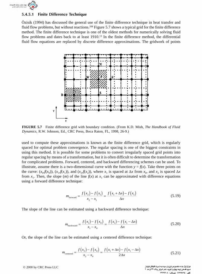
5.4.5.1 Finite Difference Technique
Özisik (1994) has discussed the general use of the finite difference technique in heat transfer andfluid flow problems, but without reactions.208 Figure 5.7 shows a typical grid for the finite differencemethod. The finite difference technique is one of the oldest methods for numerically solving fluidflow problems and dates back to at least 1910.13 In the finite difference method, the differentialfluid flow equations are replaced by discrete difference approximations. The gridwork of points
used to compute these approximations is known as the finite difference grid, which is regularlyspaced for optimal problem convergence. The regular spacing is one of the biggest constraints inusing this method. It is possible for some problems to convert irregularly spaced grid points intoregular spacing by means of a transformation, but it is often difficult to determine the transformationfor complicated problems. Forward, centered, and backward differencing schemes can be used. Toillustrate, assume there is a two-dimensional curve with the function y = f(x). Take three points onthe curve: (x0,f(x0)), (x1,f(x1)), and (x2,f(x2)), where x1 is spaced at ∆x from x0, and x2 is spaced ∆xfrom x1. Then, the slope (m) of the line f(x) at x1 can be approximated with difference equationsusing a forward difference technique:
(5.19)
The slope of the line can be estimated using a backward difference technique:
(5.20)
Or, the slope of the line can be estimated using a centered difference technique:
(5.21)
FIGURE 5.7 Finite difference grid with boundary condition. (From K.D. Mish, The Handbook of FluidDynamics, R.W. Johnson, Ed., CRC Press, Boca Raton, FL, 1998, 26-9.)
mf x f x
x x
f x x f x
xforward = ( ) − ( )−
=+( ) − ( )2 1
2 1
1 1∆∆
mf x f x
x x
f x f x x
xbackward = ( ) − ( )−
= ( ) − −( )1 0
1 0
1 1 ∆∆
mf x f x
x x
f x x f x x
xcentered = ( ) − ( )−
=+( ) − −( )2 0
2 0
1 1
2
∆ ∆∆
© 2000 by CRC Press LLC
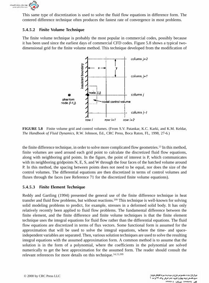
This same type of discretization is used to solve the fluid flow equations in difference form. Thecentered difference technique often produces the fastest rate of convergence in most problems.
5.4.5.2 Finite Volume Technique
The finite volume technique is probably the most popular in commercial codes, possibly becauseit has been used since the earliest days of commercial CFD codes. Figure 5.8 shows a typical two-dimensional grid for the finite volume method. This technique developed from the modification of
the finite difference technique, in order to solve more complicated flow geometries.13 In this method,finite volumes are used around each grid point to calculate the discretized fluid flow equations,along with neighboring grid points. In the figure, the point of interest is P, which communicateswith its neighboring gridpoints N, E, S, and W through the four faces of the hatched volume aroundP. In this method, the spacing between points does not need to be equal, nor does the size of thecontrol volumes. The differential equations are then discretized in terms of control volumes andfluxes through the faces (see Reference 71 for the discretized finite volume equations).
5.4.5.3 Finite Element Technique
Reddy and Gartling (1994) presented the general use of the finite difference technique in heattransfer and fluid flow problems, but without reactions.209 This technique is well-known for solvingsolid modeling problems to predict, for example, stresses in a deformed solid body. It has onlyrelatively recently been applied to fluid flow problems. The fundamental difference between thefinite element, and the finite difference and finite volume techniques is that the finite elementtechnique uses the integral equations for fluid flow rather than the differential equations. The fluidflow equations are discretized in terms of flux vectors. Some functional form is assumed for theapproximation that will be used to solve the integral equations, where the time- and space-independent variables are separated. Then, various solution techniques are used to solve the resultingintegral equations with the assumed approximation form. A common method is to assume that thesolution is in the form of a polynomial, where the coefficients in the polynomial are solvednumerically to get the best approximation for the assumed form. The reader should consult therelevant references for more details on this technique.14,15,209
FIGURE 5.8 Finite volume grid and control volumes. (From S.V. Patankar, K.C. Karki, and K.M. Keldar,The Handbook of Fluid Dynamics, R.W. Johnson, Ed., CRC Press, Boca Raton, FL, 1998, 27-6.)
© 2000 by CRC Press LLC
5.4.5.4 Mixed
Pember et al. (1995) used a hybrid discretization scheme to simulate an industrial burner.69 Theirgrid consisted of uniform rectangular cells everywhere except at the furnace walls, for which theyused finite elements to solve what they called mixed cells where the cells contained some fluidand some solid boundary. This method was termed an “embedded boundary method” and wasoffered as an alternative to using body-fitted coordinates.
5.4.5.5 None
As discussed above for the vortex methods of solution (see section 5.2.1.2), no discretization ofthe space is used to simulate the fluid flow. Instead, the properties of the vortices are tracked asthey evolve and dissipate, without regard to any grid system. This is a more accurate way ofsimulating the space as it eliminates the problems of how to discretize the space. There are alsono problems with the numerical errors associated with discretization.
5.4.6 SOLUTION METHODS
Shyy and Mittal (1998) have presented a number of common methods used to solve the Navier-Stokes equations.210 In most cases, the objective is to reduce integro-differential equations intoalgebraic equations, usually by discretization, that can then be solved in a variety of ways. Thechoice of solution method depends on the type of problem, especially as to whether the problemcan be linearized or not. Linearized equations are commonly put into matrix form and then solvedusing a variety of available matrix reduction techniques, such as the Gauss Elimination Method,the Thomas Algorithm, Gauss-Seidel Iteration, Successive Over-Relaxation, Red and Black Order-ing Scheme, or LU Decomposition. Nonlinear systems may be solved with other techniques, suchas Newton-Raphson Iteration.
5.4.7 MODEL VALIDATION
Roache (1998) has written an entire book about verification and validation of computation fluiddynamics modeling.211 He noted the distinction between verification (“solving the equations right”)and validation (“solving the right equations”). Here, no discussion will be given on verification asthis is available in any good CFD book (including the book by Roache), which as Roache notedis a more mathematical issue. For the purposes of this chapter section, it is assumed that themathematical models in a given code have been properly debugged and produce reliable resultswithin a given accuracy range. Of more concern in combustion modeling is validation, to makesure the appropriate physics are being used for the problem under consideration and that thosephysics are properly simulated. Validation is a much more difficult problem than verification,especially in combustion simulations, due to the difficulties of making relevant and accuratemeasurements in harsh environments.
One of the seductive aspects of computer modeling is that virtually any type of problem canbe simulated. How a problem is modeled depends on many things; but if enough assumptions aremade, it is possible to generate computational “results.” For the naïve and inexperienced, thetendency may be to believe anything that is generated by a computer — because, how can acomputer be wrong? The caveat, “garbage in, garbage out” definitely applies to computer modelingof complex industrial combustion problems. Any given problem may have many assumptions thatneed to be made, so the results are only as good as the model and the accompanying assumptions.Paraphrasing an anonymous researcher, “Everyone believes a computer analysis except the onewho did it, and no one believes experimental results except the one who made them.” This is tosay that most people inherently realize the difficulties of making experimental measurements incomplex geometries, but most naturally believe the results generated by a computer.
© 2000 by CRC Press LLC

As any good modeler knows, a model is only as good as its validation. Models must constantlybe tested against experimental measurements when they are applied to new problems. Modelvalidation is particularly difficult for industrial combustion problems because of the difficulty inmaking measurements in harsh environments and because of the cost involved in making thosemeasurements. Most measurements made in industrial combustors are with intrusive water-cooledprobes because many of the nonintrusive laser-based techniques have not yet been developed forlarge scales, are not rugged enough for the environments, or are too costly to use outside the lab.These intrusive probes are often larger than those used in labs because more water cooling isrequired in high-temperature combustors. Therefore, the flow is disturbed by the probes, whichmakes it more difficult to compare the measurements with the modeling results. In general, thereis relatively little experimental data available for industrial combustors that has enough informationto do a complete model validation. This is an important research need for the future — to generatecomprehensive data sets in a wide range of industrial combustion systems that can be used formodel validation. Some typical model validation cases are given next; they are representative ofthose available to date.
Fiveland et al. (1996) presented four validation cases for comparison against codes developedby Babcock and Wilcox.212 Although the codes are primarily directed at large-scale boilers, thevalidations were done for a broader range of cases, including flow in a curved duct, nonreactingflow and natural gas combustion in a swirl stabilized flame, and swirling flow coal combustion ina one-sixth scale model of a utility boiler. Kaufman and Fiveland (1995) generated a large set ofexperimental data for the swirl-stabilized natural gas flame case in the Burner Engineering ResearchLab at Sandia National Labs (Livermore, CA) as part of a program partially funded by the GasResearch Institute (Chicago, IL).213 This data was used for the model validation. The model resultswere generally very good, except in the recirculation zones. Further work was recommended toimprove the chemistry and turbulence models.
5.4.8 INDUSTRIAL COMBUSTION EXAMPLES
The two major parts of industrial combustion problems include the burners and the combustors.These are often modeled separately for a variety of reasons, as previously discussed. Examples ofmodeling different types of burners and combustors are given next.
5.4.8.1 Modeling Burners
There have been numerous papers on modeling industrial burners. A sampling of references isgiven for modeling the following industrial burners:
• Radiant tube burners214-215
• Swirl burners217
• Pulse combustion burner218
• Porous radiant burners219-224
• Industrial hydrogen sulfide burner225
Butler et al. (1986) gave a general discussion of modeling burners using the finite volume tech-niques.226 Schmücker and Leyens (1998) described the use of CFD to design a new nozzle-mixburner referred to as the Delta Burner.227 Schmidt et al. (1998) described the use of CFD to redesigna burner, originally firing on coal, to fire on natural gas for use in a rotary kiln.228
Modeling radiant burners poses the additional challenge of simulating a porous medium.229
Perrin et al. (1986) discussed the use of a numerical model for the design of a single-ended radianttube for immersion in and heating of a bath of molten zinc.230 A sample result of the temperatureand heat flux distribution from the tube is shown in Figure 5.9. As can be seen, most of the heat
© 2000 by CRC Press LLC

transfer is by radiation. Hackert et al. (1998) simulated the combustion and heat transfer in two-dimensional porous burners.231 Two different porous geometries were simulated: a honeycombconsisting of parallel, nonconnecting passages and a separated plates geometry consisting of parallel
but broken walls where there was no continuous solid path, which minimizes the importance ofsolid conduction. Spatial calculated temperatures compared favorably with measured values. Theradiant efficiency in the stable region of the flame ranged from 15% to 17% and 22% for the twogeometries, respectively. They determined a volumetric Nu of 5.4 ± 0.3, regardless of burning rateor pore size, for the separated plates geometry; this compares favorably with other values reportedin the literature. Fu et al. (1998) used a one-dimensional model to simulate the performance of aporous radiant burner.232 The model accounted for the interaction of convection, conduction, radi-ation, and chemical reaction in the burner, which consisted of two layers of reticulated ceramicshaving different porosities. The model showed that the radiant efficiency increased with the volu-metric heat transfer coefficient and the effective thermal conductivity of the solid matrix, anddecreased when the firing rate increased and the equivalence ratio decreased.
5.4.8.2 Modeling Combustors
Numerous papers have been presented over the past few decades on the modeling of industrialcombustors. Some of the earliest work was done at Imperial College (U.K.).2,233,234 A sampling ofreferences are given for modeling industrial combustors:
• General combustors and boilers235-249
• Pulse combustors250,272-274
• Glass furnaces251-256
• Aluminum reverberatory furnaces257
• Metal reheat furnaces36,258-260
• Radiant tube batch furnace261
• Flash smelting furnaces262,263
FIGURE 5.9 Predicted temperature and heat flux on the shell of a single-ended radiant tube immersed inmolten zinc. (Courtesy of the American Society of Metals, Warren, PA.230 With permission.)
© 2000 by CRC Press LLC

• Industrial coal combustors264-268
• Steam reformers for liquefied petroleum gas conversion269
• Fluid catalytic crackers270,271
• Rotary hearth calciners275
• Rotary kilns276,277
• Cement rotary kiln278
• Vertical lime kilns279
• Generic oxy/fuel-fired furnace280
• Rotary kiln incinerator281-283
• Municipal solid waste incinerator ash melting furnace284
• Hazardous waste incineration furnace285
• Baking ovens286
Carvalho and Nogueira (1997) modeled glass-melting furnaces, cement kilns, and baking ovens.287
Song and Viskanta (1986) did a parametric study of the thermal performance of a generic naturalgas-fired furnace.288 Some papers have specifically focused on radiation modeling in combustors,289
while other papers have considered swirling flows in furnaces.290,291
Carvalho and Nogueira (1993) reviewed the modeling of industrial glass melting processes.292
They noted that modeling glass melting is especially important because of the difficulty in makingmeasurements due to the very high temperatures and corrosive environment. The models are usefulfor improving glass quality, increasing thermal efficiency, reducing pollution emissions, and improv-ing equipment reliability. They recommended further research in simulating flow modeling, batchmelting, fining and refining, foam formation/elimination, homogenizing, refractories, radiativetransfer, and the mass transfer between the glass melt and the combustion chamber. Glass modelingis particularly difficult if the combustion space and molten glass are coupled together, because ofthe large disparity in flow types. The combustion space may have turbulent gas flow while themolten glass is a very low-speed flow of highly viscous material. The system is further complicatedby the transparent radiative characteristic of the glass and by the chemical reactions occurring inboth the gas space and liquid glass phase. In many cases, electrodes are located in the liquid glassand gases may be bubbled through the glass to stimulate stirring and circulation patterns in theglass. The load consists of fine solid materials at the inlet of the tank and liquid glass at the outletof the tank. Despite this complexity, models have been successfully used to further the understandingof and improvement in the glass production process.
Viskanta and co-workers did parametric computational studies of both direct- and indirect-firedfurnaces.293-296 Chapman et al. (1989) presented the results of parametric studies of a direct-fired,continuous reheating furnace.293 They developed a simplified mathematical model that accuratelycalculated the heat balance throughout the furnace. The combustion space was divided into zonesthat were considered to be well-stirred reactors. The load in each zone was further subdivided intosmaller control volumes. Radiation was modeled using Hottel’s zone method. A primary objectiveof the study was to compute the furnace thermal efficiency as a function of a variety of parameters,including the load velocity, load emissivity, furnace combustion space height, and refractory emis-sivity. The furnace efficiency increased rapidly with the initial increase in load velocity and thenleveled off with further increases in velocity. The load heat flux was relatively insensitive to theload velocity — except for the lowest speed, where the flux was considerably lower. The heat fluxto the load was most sensitive to the load emissivity, as shown in Figure 5.10. The heat flux to theload was relatively insensitive to the height of the combustion space. Although the model used inthe study was fairly simple, with no detailed fluid flow calculations, it was useful for studying awide range of values for different parameters — which makes it a valuable design tool for studyingother configurations. In a companion study, Chapman et al. (1989) also did a parametric modelingstudy of direct-fired batch reheating furnaces.294 Again it was shown that the heat flux to the load,was very sensitive to the emissivity of the load as shown in Figure 5.11. Chapman et al. (1994)
© 2000 by CRC Press LLC

FIGURE 5.10 Load heat flux as a function of the load emissivity and distance in the furnace for a direct-fired continuous reheat furnace. (Courtesy of ASME, New York.293 With permission.)
FIGURE 5.11 Load heat flux as a function of the load emissivity and distance in the furnace for a direct-fired batch reheat furnace. (Courtesy of ASME, New York.294 With permission.)
© 2000 by CRC Press LLC

modeled a direct-fired metal reheat furnace with impinging flame jets.295 The model simulated anactual steel reheat furnace at an Inland Steel Co. plant in East Chicago, Indiana. A typical result,shown in Figure 5.12, shows how the heat transfer to the load was affected by the fuel firing rate.
REFERENCES
1. R. Weber, Scaling Characteristics of aerodynamics, heat transfer, and pollutant emissions in industrialflames, Twenty-Sixth Symposium (International) on Combustion, The Combustion Institute, Pittsburgh,PA, 1996, 3343-3354.
2. S. Patankar and B. Spalding, Simultaneous predictions of flow patterns and radiation for three-dimensional flames, in Heat Transfer in Flames, N.H. Afgan and J.M. Beer, Eds., Scripta Book Co.,Washington, D.C., 1974, 73-94.
3. E.E. Khalil, Modelling of Furnaces and Combustors, Abacus Press, Kent, U.K., 1982.4. E.S. Oran and J.P. Boris, Eds., Numerical Approaches to Combustion Modeling, Vol. 135, Progress
in Astronautics and Aeronautics, American Institute of Aeronautics and Astronautics, Washington,D.C., 1991.
5. B. Larrouturou, Recent Advances in Combustion Modelling, World Scientific, Singapore, 1991.6. T.J. Chung, Numerical Modeling in Combustion, Taylor & Francis, Washington, D.C., 1993.7. D.G. Lilley, Chemically reacting flows (combustion), in The Handbook of Fluid Dynamics, R.W.
Johnson, Eds., CRC Press, Boca Raton, FL, 1998, chap. 16.8. D.B. Spalding, The art of partial modeling, Ninth Symposium (International) on Combustion, Aca-
demic Press, New York, 1963, 833-843.9. R. Weber, A.A. Peters, P.P. Breithaupt, and B.M.V. Visser, Mathematical modeling of swirling pul-
verized coal flames: What can combustion engineers expect from modeling?, Amer. Soc. of Mech.Eng. (ASME) FACT 17, 71-86, 1993.
10. E.S. Oran and J.P. Boris, Detailed modeling of combustion systems, Prog. in Energy and Comb.Science, 7(1), 1-72, 1981.
11. B.E. Launder and D.B. Spalding, The numerical computation of turbulent flows, in Lectures inMathematical Modeling of Turbulence, Academic Press, London, 1972.
12. J.I. Ramos, Finite-difference methods in turbulent combustion, in Numerical Modeling in Combustion,T.J. Chung, Ed., Taylor & Francis, Washington, D.C., 1993, 281-373.
FIGURE 5.12 Load heat flux (total, radiative and convective) as a function of the fuel firing rate for adirect-fired continuous reheat furnace. (Courtesy of Gordon & Breach, London.296 With permission.)
© 2000 by CRC Press LLC
13. K.D. Mish, Finite difference method, in The Handbook of Fluid Dynamics, R.W. Johnson, Ed., CRCPress, Boca Raton, FL, 1998, chap. 26.
14. T.J. Chung, Finite element methods in turbulent combustion, in Numerical Modeling in Combustion,T.J. Chung, Ed., Taylor & Francis, Washington, D.C., 1993, 375-397.
15. A.J. Baker, Finite element method, in The Handbook of Fluid Dynamics, R.W. Johnson, Ed., CRCPress, Boca Raton, FL, 1998, chap. 28.
16. H.A. Dwyer, Finite-volume methods in turbulent combustion, in Numerical Modeling in Combustion,T.J. Chung, Ed., Taylor & Francis, Washington, D.C., 1993, 399-408.
17. S.V. Patankar, K.C. Karki, and K.M. Keldar, Finite volume method, in The Handbook of FluidDynamics, R.W. Johnson, Ed., CRC Press, Boca Raton, FL, 1998, chap. 27.
18. G.E. Karniadakis and R.D. Henderson, Spectral element methods for incompressible flows, in TheHandbook of Fluid Dynamics, R.W. Johnson, Ed., CRC Press, Boca Raton, FL, 1998, chap. 29.
19. A.F. Ghoniem, Vortex simulation of reacting shear flow, in Numerical Approaches to CombustionModeling, E.S. Oran and J.P. Boris, Eds., Vol. 135, Progress in Astronautics and Aeronautics, AmericanInstitute of Aeronautics and Astronautics, Washington, D.C., 1991, 305-348.
20. L.-F. Martins and A.F. Ghonien, Simulation of the nonreacting flow in a bluff-body burner — Effectof the diameter ratio, in Heat and Mass Transfer in Fires and Combustion Systems, W.L. Grosshandlerand H.G. Semerjian, Eds., ASME HTD-Vol. 148, New York, 1990, 33-44.
21. C. Fureby, E. Lundgren, and S.-I. Möller, Large eddy simulation of combustion, in Tranport Phenom-ena in Combustion, Vol. 2, S.H. Chan, Ed., Taylor & Francis, Washington, D.C., 1996, 1083-1094.
22. H.G. Weller, G. Tabor, A.D. Gosman, and C. Fureby, Application of a flame-wrinkling LES combus-tion model to a turbulent mixing layer, Twenty-Seventh Symposium (International) on Combustion,The Combustion Institute, Pittsburgh, PA, 1998, 899-907.
23. G. Tryggvason and W.J.A. Dahm, An integral method for mixing, chemical reactions, and extinctionin unsteady strained diffusion layers, Comb. Flame, 83(3-4), 207-220, 1990.
24. C.H.H. Chang, W.J.A. Dahm, and G. Tryggvason, Lagrangian model simulations of molecular mixing,including finite rate chemical reactions, in temporally developing shear layer, Phys. Fluids A, 3(5),1300-1311, 1991.
25. W.J.A. Dahm, G. Tryggvason, and M. Zhuang, Intergral method solution of time-dependent straineddiffusion-reaction layers with multistep kinetics, SIAM J. Appl. Math., 56(4), 1039-1059, 1996.
26. W.J.A. Dahm, G. Tryggvason, J.A. Kezerle and R.V. Serauskas, Simulation of turbulent flow andcomplex chemistry by local integral moment (LIM) modeling, Proc. of 1995 International GasResearch Conf., D.A. Dolenc, Ed., Govt. Institutes, Rockville, MD, 1996, 2169-2178.
27. M.Y. Hussaini and T.A. Zang, Spectral Methods in Fluid Dynamics, Annu. Rev. of Fluid Mechanics,19, 339-367, 1987.
28. P.A. McMurtry and P. Givi, Spectral simulations of reacting turbulent flows, in Numerical Approachesto Combustion Modeling, E.S. Oran and J.P. Boris, Eds., Vol. 135, Progress in Astronautics andAeronautics, American Institute of Aeronautics and Astronautics, Washington, D.C., 1991, 257-303.
29. P. Givi and C.K. Madnia, Spectral methods in combustion, in Numerical Modeling in Combustion,T.J. Chung, Ed., Taylor & Francis, Washington, D.C., 1993, 409-452.
30. V. Eswaran and S.B. Pope, Direct numerical simulations of the turbulent mixing of a passive scalar,Physics of Fluids, 31(3), 506-520, 1988.
31. J.H. Chen, J.M. Card, M. Day, and S. Mahalingam, Direct numerical simulation of turbulent non-premixed methane-air flames, in Tranport Phenomena in Combustion, Vol. 2, S.H. Chan, Ed., Taylor& Francis, Washington, D.C., 1996, 1049-1060.
32. T. Poinsot, Using direct numerical simulations to understand premixed turbulent combustion, Twenty-Sixth Symposium (International) on Combustion, The Combustion Institute, Pittsburgh, PA, 1996,219-232.
33. T. Baritaud, T. Poinsot, and M. Baum, Eds., Direct Numerical Simulation for Turbulent ReactingFlows, Editions Technip, Paris, 1996.
34. M. Boger, D. Veynante, H. Boughanem, and A. Trouvé, Direct numerical simulation analysis of flamesurface density concept for large eddy simulation of turbulent premixed combustion, Twenty-SeventhSymposium (International) on Combustion, The Combustion Institute, Pittsburgh, PA, 1998, 917-925.
35. P.A. McMurtry and P. Givi, Direct numerical simulations of mixing and reaction in non-premixedhomogeneous turbulent flows, Comb. Flame, 77, 171-185, 1989.
© 2000 by CRC Press LLC
36. R.M. Davies, D.M. Lucas, B.E. Moppett, and R.A. Galsworthy, Isothermal model studies of rapidheating furnaces, J. Inst. Fuel, 44, 453-461, 1971.
37. J.T. Kuo, System simulation and control of batch-fed solid waste incinerators, in Heat Transfer inFire and Combustion Systems, W.W. Yuen and K.S. Ball, Eds., New York, ASME HTD-Vol. 272,55-62, 1994.
38. S. Singh, M. Ziolkowski, J. Sultzbaugh, and R. Viskanta, Mathematical model of a ceramic burnerradiant heater, in Fossil Fuel Combustion 1991, R. Ruiz, Ed., New York, ASME PD-Vol. 33, 111-116,1991.
39. P.A. Gillis and P.J. Smith, An evaluation of three-dimensional computational combustion and fluiddynamics for industrial furnace geometries, Twenty-Third Symposium (International) on Combustion,The Combustion Institute, Pittsburgh, PA, 1990, 981-991.
40. M. Frenklach, Reduction of chemical reaction models, in Numerical Approaches to CombustionModeling, E.S. Oran and J.P. Boris, Eds., Vol. 135, Progress in Astronautics and Aeronautics, AmericanInstitute of Aeronautics and Astronautics, Washington, D.C., 1991, 129-154.
41. C.K. Westbrook and F.L. Dryer, Simplified reaction mechanisms for the oxidation of hydrocarbonfuels in flames, Comb. Sci. Tech., 27, 31-43, 1981.
42. N. Peters, Systematic reduction of flame kinetics: principles and details, in Dynamics of ReactiveSystems, A.L. Kuhl, J.R. Bowen, J.-C. Leyer, and A. Borisov, Eds., Vol. 113, Progress in Astronauticsand Aeronautics, American Institute of Aeronautics and Astronautics, Washington, D.C., 1988, 67-86.
43. Y.S. Kocaefe, A. Charette, and M. Munger, Comparison of the various methods for analysing theradiative heat transfer in furnaces, Proceedings of the Combustion Institute Canadian Section SpringTechnical Meeting, Vancouver, Canada, May 1987, 15-17.
44. S. Bhattacharjee and W.L. Grosshandler, Effect of radiative heat transfer on combustion chamberflows, Comb. Flame, 77, 347-357, 1989.
45. Y.R. Sivathanu, J.P. Gore, and J. Dolinar, Transient scalar properties of strongly radiating flames, inHeat and Mass Transfer in Fires and Combustion Systems, W.L. Grosshandler and H.G. Semerjian,Eds., ASME HTD-Vol. 148, 45-56, 1990.
46. G. Cox, On radiant heat transfer in diffusion flames, Combust. Sci. Tech., 17, 75-78, 1977.47. V.P. Kabashnikov and G.I. Kmit, Influence of turbulent fluctuations on thermal radiation, Appl. Spect.,
31, 963-967, 1979.48. W.L. Grosshandler and P. Joulain, The effect of large scale fluctuations on flame radiation, Prog.
Astro. and Aero., Vol. 105, Part II, AIAA, Washington, D.C., 1986, 123-152.49. A.F. Sarofim, Radiative heat transfer in combustion: friend or foe, Hoyt C. Hottel Plenary Lecture,
Twenty-First Symp. (International) on Combustion, The Combustion Institute, Pittsburgh, PA, 1986, 1-23.50. R. Viskanta and M.P. Menguc, Radiation heat transfer in combustion systems, Prog. Energy Combust.
Sci., 8, 97-160, 1987.51. G.M. Faeth, J.P. Gore, S.G. Chuech, and S.M. Jeng, Radiation from turbulent diffusion flames, Annu.
Rev. Numerical Fluid Mech. & Heat Trans., C.L. Tien and T.C. Chawla, Eds., Hemisphere, New York,Vol. 2, 1-38, 1989.
52. C.J. Hoogendoorn, L. Post and J.A. Wieringa, Modelling of combustion and heat transfer in glassfurnaces, Glastech. Ber., 63(1), 7-12, 1990.
53. Y. Zhenghua and G. Holmstedt, Fast, narrow-band computer model for radiation calculations, Num.Heat Transfer, Part B, 31, 61-71, 1997.
54. W.L. Grosshandler, Radiation from Nonhomogeneous Fires, Tech. Rep. FMRC, Sept. 1979.55. W.L. Grosshandler, Radiative heat transfer in nonhomogeneous gases: a simplified approach, Int. J.
Heat Mass Transfer, 23, 1447-1459, 1980.56. W.L. Grosshandler, RADCAL: A Narrow-Band Model for Radiation Calculation in a Combustion
Environment, NIST Tech. Note 1402, April 1993.57. F. Liu, Ö.L. Gülder, and G.J. Smallwood, Non-grey gas radiative transfer analyses using the statistical
narrow-band model, Int. J. Heat Mass Transfer, 41(14), 2227-2236, 1998.58. L.A. Gritzo and J.H. Strickland, A gridless solution of the radiative transfer equation for fire and
combustion calculations, Combust. Theory Modelling, 3, 159-175, 1999.59. R.K. Ahluwalia and K.H. Im, Radiative Heat Transfer in PC Furnaces Burning Deeply Cleaned Coals,
U.S. Dept. of Energy Report DE91 006022, Argonne National Laboratory, Argonne, IL, 1990.
© 2000 by CRC Press LLC

60. R.K. Ahluwalia and K.H. Im, Spectral radiative heat-transfer in coal furnaces using a hybrid technique,J. Inst. Energy, 67, 23-29, 1994.
61. H.M. Park, R.K. Ahluwalia, and K.H. Im, Three-dimensional radiation in absorbing-emitting-scatter-ing media using the modified differential approximation, Int. J. Heat Mass Trans., 36(5), 1181-1189,1993.
62. T.L. Wilson, A three-region, moving boundary model of a furnace flame, Proceedings of the 5th Symp.On High Performance Computing, Atlanta, GA, April 1997, U.S. Dept. of Energy ReportDE97003334, Oak Ridge National Lab, TN, 1997.
63. W.A. Gray, E. Hampartsoumian, J.M. Taylor, M. Gover, and J. Sykes, Modelling of radiant heattransfer in gas-fired furnaces using a practical personal computer package, Proc. of 1992 InternationalGas Research Conf., H.A. Thompson, Ed., Govt. Institutes, Rockville, MD, 1993, 2184-2194.
64. M.D. Rumminger, R.W. Dibble, N.H. Heberle, and D.R. Crosley, Gas temperature above a porousradiant burner: comparison of measurements and model predictions, Twenty-Sixth Symposium (Inter-national) on Combustion, The Combustion Institute, Pittsburgh, PA, 1996, 1755-1762.
65. L.B. Younis and R. Viskanta, Experimental determination of the volumetric heat transfer coefficient,Int. J. Heat Mass Transfer, 36(6), 1425-1434, 1993.
66. R.M. Kendall and J.D. Sullivan, Selective and Enhanced Radiation from Porous Surface RadiantBurners, Gas Research Institute Report GRI-93/0160, Chicago, 1993.
67. R. Dibble, Univ. of CA at Berkeley, private communication, 1997.68. R.B. Bird and M.D. Graham, General equations of newtonian fluid dynamics, in The Handbook of
Fluid Dynamics, R.W. Johnson, Ed., CRC Press, Boca Raton, FL, 1998, chap. 3.69. R.B. Pember, A.S. Almgren, W.Y. Crutchfield, L.H. Howell, J.B. Bell, P. Colella, and V.E. Beckner,
An Embedded Boundary Method for the Modeling of Unsteady Combustion in an Industrial Gas-Fired Furnace, U.S. Dept. of Commerce Report No. DE96004155, Springfield, VA, 1995.
70. S.V. Patankar and D.B. Spalding, Heat and Mass Transfer in Boundary Layers: A General CalculationProcedure, second edition, Intertext Books, London, 1970.
71. S.V. Patankar, Numerical Heat Transfer and Fluid Flow, McGraw-Hill, New York, 1980.72. G.K. Batchelor, The Theory of Homogeneous Turbulence, Cambridge Univ. Press, New York, 1953.73. J.T. Davies, Turbulence Phenomena, Academic Press, New York, 1972.74. B.E. Launder and D.B. Spalding, Mathematical Models of Turbulence, Academic Press, New York,
1972.75. J.O. Hinze, Turbulence, 2nd ed., McGraw-Hill, New York, 1975.76. P. Bradshaw, Ed., Turbulence, Springer-Verlag, New York, 1978.77. W. Kollmann, Prediction Methods for Turbulent Flows, Hemisphere, Washington, D.C., 1980.78. P. Bradshaw, Engineering Calculation Methods for Turbulent Flow, Academic Press, New York, 1981.79. T. Tatsumi, Ed., Turbulence and Chaotic Phenomena in Fluids, North Holland, New York, 1984.80. M.M. Stanisic, The Mathematical Theory of Turbulence, Springer-Verlag, New York, 1985.81. M. Lesieur, Turbulence in Fluids, Dordrecht, Boston, 1987.82. H.C. Mongia, R.M.C. So, and J.H. Whitelaw, Eds., Turbulent Reactive Flow Calculations, Gordon
and Breach, New York, 1988.83. B.S. Petukhov and A.F. Polyakov, Heat Transfer in Turbulent Mixed Convection, Hemisphere, New
York, 1988.84. V.R. Kuznetsov, Turbulence and Combustion, Hemisphere, New York, 1990.85. W.D. McComb, The Physics of Fluid Turbulence, Oxford Univ. Press, Oxford, U.K., 1990.86. W. Rodi and E.N. Ganic, Eds., Engineering Turbulence Modeling and Experiments, Elsevier Science,
Amsterdam, The Netherlands, 1990.87. M. Landahl, Turbulence and Random Processes in Fluid Mechanics, Cambridge Univ. Press, Cam-
bridge, U.K., 1992.88. S.W. Churchill, Turbulent Flows, Butterworth-Heinemann, Boston, 1993.89. D.C. Wilcox, Turbulence Modeling for CFD, DCW Industries, La Cãnada, CA, 1993.90. A.J. Chorin, Vorticity and Turbulence, Springer-Verlag, New York, 1994.91. R.J. Garde, Turbulent Flow, Wiley, New York, 1994.92. U. Frisch, Turbulence, Cambridge Univ. Press, Cambridge, U.K., 1995.93. K. Hanjalic and J.C.F. Pereira, Eds., Turbulence, Heat, and Mass Transfer, Begell House, New York,
1995.
© 2000 by CRC Press LLC

94. C.J. Chen, Fundamentals of Turbulence Modeling, Taylor & Francis, Washington, D.C., 1998.95. C.G. Speziale and R.M.C. So, Turbulence modeling and simulation, in The Handbook of Fluid
Dynamics, R.W. Johnson, Ed., CRC Press, Boca Raton, FL, 1998, chap. 14.96. J. Baldyga, Turbulent Mixing and Chemical Reactions, Wiley, New York, 1999.97. D.B. Spalding, Development of the eddy-break-up model of turbulent combustion, Twentieth Sympo-
sium (International) on Combustion, The Combustion Institute, Pittsburgh, PA, 1976, 1657-1663.98. A.G. Prudnikov, Flame turbulence, Seventh Symposium (International) on Combustion, Butterworths
Scientific Publications, London, 1959, 575-582.99. D.B. Spalding, Mathematical models of turbulent flames: a review, Combust. Sci. Tech., 13(1-6), 3-25,
1976.100. K.N.C. Bray, The interaction between turbulence and combustion, Seventeenth Symposium (Interna-
tional) on Combustion, The Combustion Institute, Pittsburgh, PA, 1978, 223-233.101. K.N.C. Bray, The challenge of turbulent combustion, Twenty-Sixth Symposium (International) on
Combustion, The Combustion Institute, Pittsburgh, PA, 1996, 1-26.102. S.B. Pope, Computations of turbulent combustion: progress and challenges, Twenty-Third Symposium
(International) on Combustion, The Combustion Institute, Pittsburgh, PA, 1990, 591-612.103. W.T. Ashurst, Modeling turbulent flame propagation, Twenty-Fifth Symposium (International) on
Combustion, The Combustion Institute, Pittsburgh, PA, 1994, 1075-1089.104. W.P. Jones and J.H. Whitelaw, Modelling and measurements in turbulent combustion, Twentieth
Symposium (International) on Combustion, The Combustion Institute, Pittsburgh, PA, 1984, 233-249.105. G.M. Faeth, Heat and mass transfer in flames, in Heat Transfer 1986, Vol. 1, C.L. Tien, V.P. Carey,
and J.K. Ferrell, Eds., Proceedings of the Eighth International Heat Transfer Conf., San Francisco,1986, 151-160.
106. V.S. Arpaci, Radiative turbulence: radiation affected turbulent forced convection, in Heat Transfer inFire and Combustion Systems — 1993, B. Farouk, M.P. Menguc, R. Viskanta, C. Presser, andS. Chellaiah, Eds., New York, ASME HTD-Vol. 250, 155-160, 1993.
107. T. Yoshimoto, T. Okamoto, and T. Takagi, Numerical simulation of combustion and heat transfer ina furnace and its comparison with experiments, in Tranport Phenomena in Combustion, Vol. 2, S.H.Chan, Ed., Taylor & Francis, Washington, D.C., 1996, 1153-1164.
108. R.P. Lindstedt and E.M. Váos, Modeling of premixed turbulent flames with second moment methods,Comb. Flame, 116, 461-485, 1999.
109. N. Swaminathan and R.W. Bilger, Assessment of combustion submodels for turbulent nonpremixedhydrocarbon flames, Comb. Flame, 116, 519-545, 1999.
110. R.W. Bilger, Turbulent jet diffusion flames, Prog. Energy Combust. Sci., 1, 87-109, 1976.111. R.D. Cess and S.N. Tiwari, Infrared radiative energy transfer in gases, in Advances in Heat Transfer,
Vol. 8, J.P. Hartnett and T.F. Irvine, Eds., Academic Press, New York, 1972, 229-283.112. C.B. Ludwig, W. Malkmus, J.E. Reardon, and J.A.L. Thomson, Handbook of Infrared Radiation,
National Aeronautics and Space Administration Report SP-3080, Washington, D.C., 1973.113. T.R. Johnson and J.M. Beer, Radiative heat transfer in furnaces: further development of the zone
method of analysis, Fourteenth Symposium (International) on Combustion, The Combustion Institute,Pittsburgh, PA, 1972, 639-649.
114. J.M. Beér, Methods for calculating radiative heat transfer from flames in combustors and furnaces,in Heat Transfer in Flames, N.H. Afgan and J.M. Beer, Eds., Scripta Book Co., Washington, D.C.,1974, 29-45.
115. T.M. Lowes, H. Bartelds, M.P. Heap, S. Michelfelder, and B.R. Pai, Prediction of radiant heat fluxdistribution, in Heat Transfer in Flames, N.H. Afgan and J.M. Beer, Eds., Scripta Book Company,Washington, D.C., 1974, chap. 10, 179-190.
116. R.O. Buckius and C.L. Tien, Infrared flame radiation, Int. J. Heat Mass Transfer, 20, 93-106, 1977.117. A.L. Crosbie and R.L. Dougherty, Two-dimensional radiative transfer in cylindrical geometry with
anisotropic scattering, J. Quant. Spectrosc. Radiat. Transfer, 25(6), 551-569, 1981.118. T.F. Wall, H.T. Duong, I.M. Stewart, and J.S. Truelove, Radiative heat transfer in furnaces: flame and
furnace models of the IFRF M1- and M2-trials, Nineteenth Symposium (International) on Combustion,The Combustion Institute, Pittsburgh, PA, 1982, 537-547.
119. H. Hayasaka, A direct simulation method for the analysis of radiative heat transfer in furnaces, in HeatTransfer in Furnaces, C. Presser and D.G. Lilley, Eds., New YorkASME HTD-Vol. 74, 59-63, 1987.
© 2000 by CRC Press LLC

120. S. Bhattacharjee and W.L. Grosshandler, A simplified model for radiative source term in combustingflows, Int. J. Heat Mass Transfer, 33(3), 507-516, 1990.
121. R. Viskanta and M.P. Mengüç, Principles of radiative heat transfer in combustion systems, in Handbookof Heat and Mass Transfer, N. Cheremisinoff, Ed., Gulf Publishing, Houston, 1990, Vol. 4, chap. 22,925-978.
122. W. Komornicki and J. Tomeczek, Modification of the wide-band gas radiation model for flamecalculation, Int. J. Heat Mass Transfer, 35(7), 1667-1672, 1992.
123. A. Soufiani and E. Djavdan, A comparison between weighted sum of gray gases and statistical narrow-band radiation models for combustion applications, Comb. Flame, 97, 240-250, 1994.
124. N. Lallemant, A. Sayre, and R. Weber, Evaluation of emissivity correlations for H2O-CO2-N2/airmixtures and coupling with solution methods of the radiative transfer equation, Prog. Energy Combust.Sci., 22, 543-574, 1996.
125. D.K. Edwards, Molecular gas band radiation, in Advances in Heat Transfer, Vol. 12, T.F. Irvine andJ.P. Hartnett, Eds., Academic Press, New York, 1976, 115-193.
126. A.T. Modak, Exponential wide band parameters for the pure rotational band of water vapor, J. Quant.Spectosc. Radiat. Transfer, 21(2), 131-142, 1979.
127. M.G. Carvalho and T.L. Farias, Modelling of heat transfer in radiating and combusting systems, Trans.IChemE, 76A, 175-184, 1998.
128. H.C. Hottel and A.F. Sarofim, Radiative Transfer, McGraw-Hill, New York, 1967.129. J.R. Howell and M. Perlmutter, Monte Carlo solution of thermal transfer through radiant media
between gray walls, J. Heat Transfer, 86(1), 116–122, 1964.130. H.C. Hamaker, Philips Research Reports 3, 103, 112, and 142, 1947.131. A.D. Gosman and F.C. Lockwood, Incorporation of a flux model for radiation into a finite difference
procedure for furnace calculations, Fourteenth Symp. (International) on Combustion, the CombustionInstitute, Pittsburgh, PA, 1973, 661-671.
132. T.M. Lowes, H. Bartelds, M.P. Heap, S. Michelfelder and B.R. Pai, Prediction of radiant heat fluxdistributions, Int. Flame Research Found. Report GO2/A/26, IJmuiden, The Netherlands, 1973.
133. W. Richter and R. Quack, A mathematical model of a low-volatile pulverised fuel flame, in HeatTransfer in Flames, N.H. Afgan and J.M. Beer, Eds., Scripta Book Co., Washington, D.C., 1974, 95-110.
134. R.G. Siddall and N. Selçuk, Two-flux modelling of two-dimensional radiative transfer in axi-sym-metrical furnaces, J. Inst. Fuel, 49, 10-20, 1976.
135. R.G. Siddall and N. Selçuk, Evaluation of a new six-flux model for radiative transfer in rectangularenclosures, Trans. IChem, 57, 163-169, 1979.
136. R. Viskanta, Radiative transfer and interaction of convection with radiation heat transfer, Advancesin Heat Transfer, T.F. Irvine and J.P. Hartnett, Eds., 1966, 175-252.
137. S. Chandrasekhar, Radiative Transfer, Dover Publications, New York, 1960.138. W.A. Fiveland, Discrete-ordinates solutions of the radiative transport equation for rectangular enclo-
sures, J. Heat Transfer, 106, 699-706, 1984.139. A.S. Jamaluddin and P.J. Smith, Predicting radiative transfer in rectangular enclosures using the
discrete ordinates method, Comb. Sci. Tech., 59(4-6), 321-340, 1988.140. A.S. Jamaluddin and P.J. Smith, Predicting radiative transfer in axisymmetric cylindrical enclosures
using the discrete ordinates method, Comb. Sci. Tech., 62(4-6), 173-186, 1988.141. W.A. Fiveland and A.S. Jamaluddin, Three-dimensional spectral radiative heat transfer solutions by
the discrete-ordinates method, in Heat Transfer Phenomena in Radiation, Combustion, and Fires,R.K. Shah, Ed., New York, ASME HTD-Vol. 106, 43-48, 1989.
142. G.D. Raithby and E.H. Chui, A finite-volume method for predicting radiant heat transfer in enclosureswith participating media, J. Heat Transfer, 112, 414-423, 1990.
143. J.C. Chai, H.S. Lee, and S.V. Patankar, Finite volume method for radiation heat transfer, J. Thermo-physics & Heat Transfer, 8(3), 419-425, 1994.
144. N.G. Shah, New Method of Computation of Radiative Heat Transfer in Combustion Chambers, Ph.D.thesis, Imperial College, London, 1979.
145. F.C. Lockwood and N.G. Shah, A new radiation solution method for incorporation in general com-bustion prediction procedures, Eighteenth Symp. (International) on Combustion, the CombustionInstitute, Pittsburgh, PA, 1981, 1405-1414.
© 2000 by CRC Press LLC

146. P. Docherty and M. Fairweather, Predictions of radiative transfer from nonhomogeneous combustionproducts using the discrete transfer method, Comb. Flame, 71, 79-87, 1988.
147. M.H.N. Naraghi and M. Kassemi, Radiative transfer in rectangular enclosures: a discretized exchangefactor solution, ASME Proceedings of the 1988 National Heat Transfer Conf., H.R. Jacobs, Ed., NewYork, 1, 259-267, 1988.
148. M.H.N. Naraghi, Radiative heat transfer in non-rectangular enclosures, in Heat Transfer Phenomenain Radiation, Combustion, and Fires, R.K. Shah, Ed., New York, ASME HTD-Vol. 106, 17-25, 1989.
149. M.H.N. Naraghi and B. Litkouhi, Discrete exchange factor solution of radiative heat transfer in three-dimensional enclosures, in Heat Transfer Phenomena in Radiation, Combustion, and Fires, R.K. Shah,Ed., New York, ASME HTD-Vol. 106, 221-229, 1989.
150. M.K. Denison and B.W. Webb, A spectral line-based weighted-sum-of-gray-gases model for arbitraryRTE solvers, J. Heat Transfer, 115, 1004-1012, 1993.
151. R.G. Siddall and N. Selcuk, The application of flux methods to prediction of the behavior of a processgas heater, in Heat Transfer in Flames, N.H. Afgan and J.M. Beer, Eds., Scripta Book Company,Washington, D.C., 1974, chap. 11, 191-200.
152. L.D. Cloutman and L. Brookshaw, Numerical Simulation of Radiative Heat Loss in an ExperimentalBurner, Lawrence Livermore National Lab, U.S. Dept. of Energy Report UCRL-JC-115048, 1993.
153. A.M. Abdullin and D.V. Vafin, Numerical investigation of the effect of the radiative properties of atube waterwall and combustion products on heat transfer in tube furnaces, J. Eng. Physics andThermophysics, 65(2), 752-757, 1994.
154. R.K. Ahluwalia and K.H. Im, Radiative Heat Transfer in Coal Furnaces, U.S. Dept. of Energy ReportDE92018770, Argonne National Lab, IL, 1992.
155. W.A. Fiveland and A.S. Jamaluddin, Three-dimensional spectral radiative heat transfer solutions bythe discrete-ordinate method, J. Thermophysics, 5(3), 335-339, 1991.
156. M.F. Modest, Modified differential approximation for radiative transfer in general three-dimensionalmedia, J. Thermophysics, 3(3), 283-288, 1989.
157. T.H. Song and R. Viskanta, Interaction of radiation with turbulence: application to a combustionsystem, J. Thermophysics, 1(1), 56-62, 1987.
158. Ü.Ö. Köylü and G.M. Faeth, Radiative properties of flame-generated soot, J. Heat Transfer, 115,409-417, 1993.
159. C.L. Tien and S.C. Lee, Flame radiation, Prog. Energy Combust. Sci., 8, 41-59, 1982.160. W.H. Dalzell, G.C. Williams, and H.C. Hottel, A light scattering method for soot concentration
measurements, Comb. Flame, 14, 161-170, 1970.161. J.E. Martin and A.J. Hurd, Scattering from fractals, J. Appl. Cryst., 20, 61-78, 1987.162. N.W. Bressloff, J.B. Moss, and P.A. Rubini, CFD prediction of couple radiation heat transfer and soot
production in turbulent flames, Twenty-Sixth Symposium (International) on Combustion, The Com-bustion Institute, Pittsburgh, PA, 1996, 2379-2386.
163. X.S. Bai, M. Balthasar, F. Mauss, and L. Fuchs, Detailed soot modeling in turbulent jet diffusionflames, Twenty-Seventh Symposium (International) on Combustion, The Combustion Institute, Pitts-burgh, PA, 1998, 1623-1630.
164. S.J. Brookes and J.B. Moss, Predictions of soot and thermal radiation properties in confined turbulentjet diffusion flames, Comb. Flame, 116, 486-503, 1999.
165. D.K. Edwards, L.K. Glassen, W.S. Hauser, and J.S. Tuchscher, Radiation heat transfer in nonisothermalnongray gases, J. Heat Transfer, 86C, 219-229, 1967.
166. B. Leckner, Spectral and total emissivity of water vapor and carbon dioxide, Comb. Flame, 19, 33-48,1972.
167. J. Taine, A line-by-line calculation of low-resolution radiative properties of CO2-CO transparent noniso-thermal gaseous mixtures up to 3000K, J. Quant. Spectroscopic Radiative Transfer, 30, 371-379, 1983.
168. J.M. Hartmann, L. Leon, and J. Taine, Line-by-line and narrow-band statistical model calculationsfor H2O, J. Quant. Spectroscopic and Radiative Transfer, 32(2), 1984, 119-127.
169. R.M. Goody, Atmospheric Radiation, Vol. I, Oxford Univ. Press, Oxford, U.K., 1964.170. G. Song, T. Bjørge, J. Holen, and B.F. Magnussen, Simulation of fluid flow and gaseous radiation
heat transfer in a natural gas-fired furnace, Int. J. Num. Methods for Heat & Fluid Flow, 7(2/3),169-180, 1997.
© 2000 by CRC Press LLC

171. R.K. Ahluwalia and K.H. Im, Spectral radiative heat-transfer in coal furnaces using a hybrid technique,J. Institute of Energy, 67, 23-29, 1994.
172. R.J. Kee, R.M. Rupley, and J.A. Miller, CHEMKIN-II: A Fortran Chemical Kinetics Package for theAnalysis of Gas Phase Chemical Kinetics, Sandia National Laboratory Report SAND89-8009B,Livermore, CA, 1989.
173. C.T. Bowman, R.K. Hanson, D.F. Davidson, W.C. Gardiner, V. Lissianski, G.P. Smith, D.M. Golden,M. Frenklach, and M. Goldberg, http://www.me.berkeley.edu/gri_mech/, 1999.
174. W.G. Mallard, F. Westley, J.T. Herron, R.F. Hampson, and D.H. Frizzell, NIST Chemical KineticsDatabase User’s Guide — Windows Version 2Q98, National Institute of Standards and Technology,Washington, D.C., 1998.
175. D.L. Baulch, C.J. Cobos, R.A. Cox, C. Esser, P. Frank et al., Evaluated kinetic data from combustionmodelling, J. Phys. Chem. Ref. Data, 21(3), 411-734, 1992.
176. D.L. Baulch, C.J. Cobos, R.A. Cox, P. Frank, G. Hayman, Th. Just, J.A. Kerr, T. Murrells, M.J. Pilling,J. Troe, R.W. Walker, and J. Warnatz, Summary table of evaluated kinetic data for combustionmodeling: Supplement 1, Comb. Flame, 98, 59-79, 1994.
177. A. Turbiez, P. Desgroux, J.F. Pauwels, L.R. Sochet, S. Poitou, and M. Perrin, GDF.kin®: a new steptowards a detailed kinetic mechanism for natural gas combustion modeling, Proceedings of the 1998International Gas Research Conf., Vol. V: Industrial Utilization, D.A. Dolenc, Ed., Gas ResearchInstitute, Chicago, 1998, 210-221.
178. W.C. Gardiner, Ed., Combustion Chemistry, Springer-Verlag, New York, 1984.179. T.M. Sloane, The Chemistry of Combustion Processes, Amer. Chem. Soc., Washington, D.C., 1984.180. P.A. Libby and F.A. Williams, Eds., Turbulent Reacting Flows, Academic Press, London, 1994.181. D.M. Golden, Evaluation of chemical thermodynamics and rate parameters for use in combustion
modeling, in Fossil Fuel Combustion, W. Bartok and A.F. Sarofim, Eds., Wiley, New York, 1991, chap. 2.182. C.K. Westbrook and F.L. Dryer, Chemical kinetics and modeling of combustion processes, Eighteenth
Symposium (International) on Combustion, The Combustion Institute, Pittsburgh, PA, 1980, 749-767.183. F. Kaufman, Chemical kinetics and combustion: intricate paths and simple steps, Nineteenth Sympo-
sium (International) on Combustion, The Combustion Institute, Pittsburgh, PA, 1982, 1-10.184. J. Wofrum, Chemical kinetics in combustion systems: the specific effect of energy, collisions, and
transport processes, Twentieth Symposium (International) on Combustion, The Combustion Institute,Pittsburgh, PA, 1984, 559-573.
185. S.W. Benson, Combustion, a chemical and kinetic view, Twenty-First Symposium (International) onCombustion, The Combustion Institute, Pittsburgh, PA, 1986, 703-711.
186. V.Y. Basevich, Chemical kinetics in the combustion process, in Handbook of Heat and Mass Transfer,N. Cheremisinoff, Ed,, Gulf Publishing, Houston, 1990, Vol. 4, chap. 18.
187. P. Gray, Chemistry and Combustion, Twenty-Third Symposium (International) on Combustion, TheCombustion Institute, Pittsburgh, PA, 1990, 1-19.
188. F.L. Dryer, The phenomenology of modeling combustion chemistry, in Fossil Fuel Combustion,W. Bartok and A.F. Sarofim, Eds., Wiley, New York, 1991, chap. 3.
189. E. Ranzi, A. Sogaro, P. Gaffuri, G. Pennati, C.K. Westbrook, and W.J. Pitz, A new comprehensivereaction mechanism for combustion of hydrocarbon fuels, Comb. Flame, 99, 201-211, 1994.
190. H.C. Magel, U. Schnell and K.R.G. Hein, Simulation of detailed chemistry in a turbulent combustorflow, Twenty-Sixth Symposium (International) on Combustion, The Combustion Institute, Pittsburgh,PA, 1996, 67-74.
191. J.A. Miller, Theory and modeling in combustion chemistry, Twenty-Sixth Symposium (International)on Combustion, The Combustion Institute, Pittsburgh, PA, 1996, 461-480.
192. A.Y. Federov, V.A. Frost, and V.A. Kaminsky, Turbulent transfer modeling in flows with chemicalreactions, in Tranport Phenomena in Combustion, Vol. 2, S.H. Chan, Ed., Taylor & Francis, Wash-ington, D.C., 1996, 933-944.
193. S.B. Pope, PDF methods for turbulent reactive flows, Prog. Energy Combust. Sci., 11(2), 119-192,1985.
194. W.P. Jones and M. Kakhi, PDF modeling of finite-rate chemistry effects in turbulent nonpremixed jetflames, Comb. Flame, 115, 210-229, 1998.
195. V. Saxena and S.B. Pope, PDF simulations of turbulent combustion incorporating detailed chemistry,Comb. Flame, 117, 340-350, 1999.
© 2000 by CRC Press LLC

196. P.J. Coelho and M.G. Carvalho, Modelling of soot formation in turbulent diffusion flames, in HeatTransfer in Fire and Combustion Systems, W.W. Yuen and K.S. Ball, Eds., New York, ASME HTD-Vol. 272, 29-39, 1994.
197. I.M. Khan and G. Greeves, A method for calculating the formation and combustion of soot in dieselengines, in Heat Transfer in Flames, N.H. Afgan and J.M. Beer, Eds., Scripta Book Co., 1974, chap. 25.
198. C.D. Stewart, K.J. Syed, and J.B. Moss, Modelling soot formation in non-premixed kerosene-airflames, Comb. Sci. Tech., 75, 211-266, 1991
199. B.F. Magnussen and B.H. Hjertager, On mathematical modelling of turbulent combustion with specialemphasis on soot formation and combustion, Sixteenth Symp. (International) on Combustion, TheCombustion Institute, Pittsburgh, PA, 1977, 719-728.
200. K.B. Lee, M.W. Thring, and J.M. Beer, On the rate of combustion of soot in a laminar soot flame,Comb. Flame, 6, 137-145, 1962.
201. J. Nagle and R.F. Strickland-Constable, Oxidation of carbon between 1000-2000C, Proc. 5th Conf.on Carbon, Pergamon Press, 1, 154, 1961.
202. M.A. Delichatsios and L. Orloff, Effects of turbulence on flame radiation from diffusion flames,Twenty-Second Symposium (International) on Combustion, The Combustion Institute, Pittsburgh, PA,1988, 1271-1279.
203. P. Boerstoel, T.H. van der Meer, and C.J. Hoogendoorn, Numerical simulation of soot-formation and-oxidation in high temperature furnaces, in Tranport Phenomena in Combustion, Vol. 2, S.H. Chan,Ed., Taylor & Francis, Washington, D.C., 1996, 1025-1036.
204. R. Said, A. Garo and R. Borghi, Soot formation modeling for turbulent flames, Combust. Flame, 108,71-86, 1997.
205. F. Xu, K.-C. Lin, and G.M. Faeth, Soot formation in laminar premixed methane/oxygen flames atatmospheric pressure, Combust. Flame, 115, 195-209, 1998.
206. M. Frenklach and H. Wang, Detailed modeling of soot particle nucleation and growth, Twenty-ThirdSymposium (International) on Combustion, The Combustion Institute, Pittsburgh, PA, 1990, 1559-1566.
207. K.M. Leung and R.P. Lindstedt, Detailed kinetic modeling of C1C3 alkane diffusion flames, Combust.Flame, 102(1-2), 129-160, 1995.
208. M.N. Özisik, Finite Difference Methods in Heat Transfer, CRC Press, Boca Raton, FL, 1994.209. J.N. Reddy and D.K. Gartling, The Finite Element Methods in Heat Transfer and Fluid Dynamics,
CRC Press, Boca Raton, FL, 1994.210. W. Shyy and R. Mittal, Solution Methods for the Incompressible Navier-Stokes Equations, Chapter 31
in The Handbook of Fluid Dynamics, R.W. Johnson, Ed., CRC Press, Boca Raton, FL, 1998.211. P.J. Roache, Verification and Validation in Computational Science and Engineering, Hermosa Pub-
lishers, Albuquerque, NM, 1998.212. W.A. Fiveland, K.C. Kaufman, and J.P. Jessee, Validation of an Industrial Flow and Combustion
Model, in Computational Heat Transfer in Combustion Systems, M.Q. McQuay, W. Schreiber,E. Bigzadeh, K. Annamalai, D. Choudhury, and A. Runchal, Ed., ASME Proceedings of the 31st AnnualNational Heat Transfer Conf., Vol. 6, New York, ASME HTD-Vol. 328, 147-157, 1996.
213. K.C. Kaufman and W.A. Fiveland, Pilot Scale Data Collection and Burner Model Numerical CodeValidation, topical report for Gas Research Institute Contract 5093-260-2729, 1995.
214. A.M. Lankhorst and J.F.M. Velthuis, Ceramic Recuperative Radiant Tube Burners: Simulations andExperiments, in Tranport Phenomena in Combustion, Vol. 2, S.H. Chan, Ed., Taylor & Francis,Washington, D.C., 1996, 1330-1341.
215. F. Mei and H. Meunier, Numerical and experimental investigation of a single ended radiant tube, inASME Proceedings of the 32nd National Heat Transfer Conf., Vol. 3: Fire and Combustion, L. Gritzoand J.-P. Delplanque, Eds., ASME, New York, 1997, 109-118.
216. H. Ramamurthy, S. Ramadhyani, and R. Viskanta, Development of fuel burn-up and wall heat transfercorrelations for flows in radiant tubes, Num. Heat Transfer, Part A, 31, 563-584, 1997.
217. S. Bortz and A. Hagiwara, Inviscid model for the prediction of the near field region of swirl burners,in Industrial Combustion Technologies, M.A. Lukasiewicz, Ed., American Society of Metals, Warren,PA, 1986, 89-97.
218. Y. Tsujimoto and N. Machii, Numerical analysis of pulse combustion burner, Twenty-First Symposium(International) on Combustion, The Combustion Institute, Pittsburgh, PA, 1986, 539-546.
© 2000 by CRC Press LLC
219. T.W. Tong, S.B. Sathe, and R.E. Peck, Improving the performance of porous radiant burners throughuse of sub-micron size fibers, in Heat Transfer Phenomena in Radiation, Combustion, and Fires, R.K.Shah, Ed., New York, ASME HTD-Vol. 106, 257-264, 1989.
220. S.B. Sathe, R.E. Peck, and T.W. Tong, A numerical analysis of combustion and heat transfer in porousradiant burners, Int. J. Heat Mass Transfer, 33(6), 1331-1338, 1990.
221. S.H. Chan and K. Kumar, Analytical investigation of SER recuperator performance, in Fossil FuelCombustion Symposium 1990, S. Singh, Ed., New York, ASME PD-Vol. 30, 161-168, 1990.
222. P.-F. Hsu, J.R. Howell, and R.D. Matthews, A numerical investigation of premixed combustion withinporous inert media, J. Heat Transfer, 115(3), 744-750, 1993.
223. R. Mital, J.P. Gore, R. Viskanta, and S. Singh, Radiation efficiency and structure of flames stabilizedinside radiant porous ceramic burners, in Combustion and Fire, M.Q. McQuay, W. Schreiber,E. Bigzadeh, K. Annamalai, D. Choudhury and A. Runchal, Eds., ASME Proceedings of the 31st
National Heat Transfer Conf., Vol. 6, ASME HTD-Vol. 328, 131-137, New York, 1996.224. C.L. Hackert, J.L. Ellzey, and O.A. Ezekoye, Numerical simulation of a porous honeycomb burner,
in ASME Proceedings of the 32nd National Heat Transfer Conf., Vol. 3: Fire and Combustion, L. Gritzoand J.-P. Delplanque, Eds., ASME, New York, 1997, 147-153.
225. M.M. Sidawi, B. Farouk, and U. Parekh, A numerical study of an industrial hydrogen sulfide burnerwith air- and oxygen-based operations, in Heat Transfer in Fire and Combustion Systems — 1993, B.Farouk, M.P. Menguc, R. Viskanta, C. Presser and S. Chellaiah, Eds., New York, ASME HTD-Vol. 250,227-234, 1993.
226. G.W. Butler, J. Lee, K. Ushimaru, S. Bernstein, and A.D. Gosman, A numerical simulation method-ology and its application in natural gas burner design, in Industrial Combustion Technologies, M.A.Lukasiewicz, Ed., American Society of Metals, Warren, PA, 109-116, 1986.
227. A. Schmücker and R.E., Leyens, Development of the delta burner using computational fluid dynamics,Proc. of 1998 International Gas Research Conf., Vol. V: Industrial Utilization, D.A. Dolenc, Ed., GasResearch Institute, Chicago, 1998, 516-526.
228. B. Schmidt, B. Spiegelhauer, N.B. Kampp Rasmussen, and F. Giversen, Development of a processadapted gas burner through mathematical modelling and practical experience, Proc. of 1998 Interna-tional Gas Research Conf., Vol. V: Industrial Utilization, D.A. Dolenc, Ed., Gas Research Institute,Chicago, 1998, 578-584.
229. J.R. Howell, M.J. Hall, and J.L. Ellzey, Combustion within porous media, in Heat Transfer in PorousMedia, Y. Bayazitoglu and U.B. Sathuvalli, Eds., New York, ASME, HTD-Vol. 302, 1-27, 1995.
230. M. Perrin, P. Lievoux, R. Borghi, and M. Gonzalez, Utilization of a numerical model for the designof a gas immersion tube, in Industrial Combustion Technologies, M.A. Lukasiewicz, Ed., Amer. Soc.Metals, Warren, PA, 1986, 127-134.
231. C.L. Hackert, J.L. Ellzey, and O.A. Ezekoye, Combustion and heat transfer in model two-dimensionalporous burners, Comb. Flame, 116, 177-191, 1999.
232. X. Fu, R. Viskanta, and J.P. Gore, Modeling of thermal performance of a porous radiant burner, inCombustion and Radiation Heat Transfer, R.A. Nelson, K.S. Ball, and Z.M. Zhang, Eds., Proceedingsof the ASME Heat Transfer Division — 1998, Vol. 2, ASME HTD-Vol. 361-2, 11-19, New York, 1998.
233. S.V. Patankar and D.B. Spalding, A computer model for three-dimensional flows in furnaces, Four-teenth Symposium (International) on Combustion, The Combustion Institute, Pittsburgh, PA, 1973,605-614.
234. L.S. Caretto, A.D. Gosman, S.V. Patankar, and D.B. Spalding, Two calculation procedures for steady,three-dimensional flows with recirculation, in proc. 3rd Int. Conf. On Numerical Methods in FluidDynamics, Springer, Berlin, 1972, 60-68.
235. S.V. Patankar and D.B. Spalding, A computer model for three-dimensional flow in furnaces, FourteenthSymposium (International) on Combustion, The Combustion Institute, Pittsburgh, PA, 1972, 605-614.
236. T.M. Lowes, M.P. Heap, S. Michelfelder, and B.R. Pai, Paper 5. Mathematical modelling of combustionchamber performance, J. Institute Fuel, 46(38), 343-351, 1973.
237. W. Richter, Prediction of heat and mass transfer in a pulverised fuel furnace, Letters in Heat & MassTransfer, 1, 83-94, 1978.
238. M.M.M. Abou Ellail, A.D. Gosman, F.C. Lockwood, and I.E.A. Megahed, Description and validationof a three-dimensional procedure for combustion chamber flows, J. Energy, 2(2), 71-80, 1978.
© 2000 by CRC Press LLC

239. A.D. Gosman, F.C. Lockwood, and A.P. Salooja, The prediction of cylindrical furnaces gaseous fueledwith premixed and diffusion burners, Seventeenth Symposium (International) on Combustion, TheCombustion Institute, Pittsburgh, PA, 1978, 747-760.
240. E.E. Khalil, P. Hutchinson, and J.H. Whitelaw, The calculation of the flow and heat-transfer charac-teristics of gas-fired furnaces, Eighteenth Symposium (International) on Combustion, The CombustionInstitute, Pittsburgh, PA, 1980, 1927-1938.
241. K. Görner, Prediction of the turbulent flow, heat release and heat transfer in utility boiler furnaces,in Coal Combustion, J. Feng, Ed., Hemisphere Publishing, New York, 1988, 273-282.
242. K. Görner and W. Zinser, Prediction of three-dimensional flows in utility boiler furnaces and com-parison with experiments, Comb. Sci. Tech., 58, 43-58, 1988.
243. P.A. Gillis and P.J. Smith, An evaluation of three-dimensional computational combustion and fluiddynamics in industrial furnace geometries, in Twenty-Third Symp. (International) on Combustion, TheCombustion Institute, Pittsburgh, PA, 1990, 981-991.
244. M.G. Carvalho, J.B. Lopes, and M. Nogueira, A three-dimensional procedure for combustion andheat transfer in industrial furnaces, in Advanced Computational Methods in Heat Transfer, Vol. 3:Phase Change and Combustion Simulation, L.C. Wrobel, C.A. Brebbia, and A.J. Nowak, Eds.,Springer-Verlag, Berlin, 1990, 171-183.
245. H. Meunier, Modelling of industrial furnaces, proc. of 2nd European Conf. On Industrial Furnacesand Boilers, Portugal, April, R. Collin, W. Leuckel, A. Reis, and J. Ward, Eds., 1991, 1-21.
246. J.M. Rhine and R.J. Tucker, Modelling of Gas-fired Furnaces and Boilers and Other Industrial HeatingProcesses, British Gas and McGraw-Hill, New York, 1991.
247. V. Sidlauskas and M. Tamonis, Mathematical modeling of the thermal process in industrial combustionchambers, Heat Transfer — Soviet Research, 23(7), 897-914, 1991.
248. M. Matsumura, S. Ito, Y. Ichiraku, and T. Saeki, Heat transfer simulation in industrial gas furnaces,Proc. of 1992 International Gas Research Conf., H.A. Thompson, Ed., Govt. Institutes, Rockville,MD, 1993, 2195-2204.
249. C.J. Hoogendoorn, Full modelling of industrial furnaces and boilers, in Tranport Phenomena inCombustion, Vol. 2, S.H. Chan, Ed., Taylor & Francis, Washington, D.C., 1996, 1177-1188.
250. P.K. Barr, J.O. Keller, and J.A. Kezerle, SPCDC: a user-friendly computation tool for the design andrefinement of practical pulse combustion systems, Proc. of 1995 International Gas Research Conf.,D.A. Dolenc, Ed., Government Institutes, Rockville, MD, 1996, 2150-2159.
251. A.D. Gosman, F.C. Lockwood, I.E.A. Megahed, and N.G. Shah, The prediction of the flow, reactionand heat transfer in the combustion chamber of a glass furnace, in AIAA 18th Aerospace SciencesMeeting, January, Pasadena, CA, 1980, 14-46.
252. L. Post and C.J. Hoogendoorn, Heat Transfer in Gas-Fired Glass Furnaces, VDI, Berichte, No. 645,457-466, 1987.
253. C.J. Hoogendoorn, L. Post, and J.A. Wieringa, Modelling of combustion and heat transfer in glassfurnaces, Glastech. Ber., 63(1), 7-12, 1990.
254. V.B. Kut’in, S.N. Gushchin, and V.G. Lisienko, Heat transfer in the cross-fired glass furnace, Glass& Ceramics, 54(5-6), 135-138, 1997.
255. M.G. Carvalho, M. Nogueira and J. Wang, Mathematical modelling of the glass melting industrialprocess, in Proc. XVII Int. Congress on Glass, Beijing, China, International Academic Publishers, 6,69-74, 1995.
256. V.B. Kut’in, S.N. Gushchin, and V.G. Lisienko, Heat exchange in the cross-fired glass furnace, Glass& Ceramics, 54(5-6), 172-174, 1997.
257. V.Y. Gershtein and C.E. Baukal, Model prediction comparison for aluminum reverberatory furnacefiring on air-, air-oxy-, and oxy/fuel, presented at 1999 The Minerals, Metals & Materials SocietyAnnual Meeting & Exhibition, February 28–March 4, 1999, San Diego, CA.
258. Y.K. Lee, H.S. Park, and K.W. Cho, Effect of fuel gas preheating on combustion and heat transfer inreheating furnace, Proceedings of the 13th Energy Engineering World Congress, Energy & Environ-mental Strategies for the 1990s, Atlanta, GA, October 1990, 1991, chap. 78, 461-466.
259. R. Klima, Improved knowledge of gas flow and heat transfer in reheating furnaces, Scandinavian J.Metallurgy (Suppl.), 26, 25-32, 1997.
260. J.M. Blanco and J.M. Sala, Improvement of the efficiency and working conditions for reheatingfurnaces through computational fluid dynamics, Industrial Heating, LXVI(5), 63-67, 1999.
© 2000 by CRC Press LLC

261. H. Ramamurthy, S. Ramadhyani, and R. Viskanta, Thermal system model for a radiant tube batchreheating furance, Proc. of 1992 International Gas Research Conf., H.A. Thompson, Ed., Govt.Institutes, Rockville, MD, 1993, 2205-2216.
262. N.D.H. Munroe, Experimental and numerical modeling of transport phenomena in a particulatereacting system, in Heat Transfer in Fire and Combustion Systems — 1993, B. Farouk, M.P. Menguc,R. Viskanta, C. Presser, and S. Chellaiah, Eds., New York, ASME HTD-Vol. 250, 69-78, 1993.
263. T. Ahokainen, A. Jokilaakso, O. Teppo, and Y. Yang, Flow and Heat Transfer Simulation in a FlashSmelting Furnace, NTIS Report DE95779247, U.S. Dept. of Commerce, Springfield, VA, 1994.
264. D.L. Smoot, Pulverized coal diffusion flames: a perspective through modelling, in Eighteenth Symp.(International) on Combustion, The Combustion Institute, Pittsburgh, PA, 1981, 1185-1202.
265. W.A. Fiveland and R.A. Wessel, Numerical model for predicting performance of three-dimensionalpulverized-fuel fired furnaces, ASME J. Engng. Gas Turbines and Power, Vol. 110, 117-126, 1988.
266. S. Li, B. Yu, W. Yao, and W. Song, Numerical modelling for pulverised coal combustion in largefurnace, in Proc. 2nd Int. Symp. On Coal Combustion, Beijing, China, X. Xu, L. Zhou, and W. Fu,Eds., China Machine Press, Beijing, China, 1991, 167-173.
267. R. Boyd and A. Lowe, Three-dimensional modelling of a pulverised coal fired utility furnace, in CoalCombustion, Hemisphere, New York, 1988, 165-172.
268. B.S. Brewster, S.C. Hill, P.T. Radulovic, and L.D. Smoot, Comprehensive modeling, in Fundamentalsof Coal Combustion for Clean and Efficient Use, L.D. Smoot, Ed., Elsevier, Amsterdam, 1993, chap. 8.
269. K. Kudo, H. Taniguchi, and K. Guo, Heat-transfer simulation in a furnace for steam reformer, HeatTransfer — Japanese Research, 20(8), 750-764, 1992.
270. K.N. Theologos and N.C. Markatos, Advanced modeling of fluid catalytic cracking riser-type reactors,AIChE J., 36(6), 1007-1017, 1993.
271. S.L. Chang, C.Q. Zhou, S.A. Lottes, B. Golchert, and M. Petrick, A numerical investigation of thescaled-up effects on flow, heat transfer, and kinetics processes of FCC units, in Combustion andRadiation Heat Transfer, R.A. Nelson, K.S. Ball, and Z.M. Zhang, Eds., Proceedings of the ASMEHeat Transfer Division — 1998, Vol. 2, ASME HTD-Vol. 361-2, 73-81, 1998.
272. B. Ponizy and S. Wojcicki, On modeling of pulse combustors, Twentieth Symposium (International)on Combustion, The Combustion Institute, Pittsburgh, PA, 1984, 2019-2024.
273. P.K. Barr and H.A. Dwyer, Pulse combustor dynamics: a numerical study, in Numerical Approachesto Combustion Modeling, E.S. Oran and J.P. Boris, Eds., Vol. 135, Progress in Astronautics andAeronautics, American Institute of Aeronautics and Astronautics, Washington, D.C., 1991, 673-710.
274. E. Lundgren, U. Marksten, and S.-I. Möller, The enhancement of heat transfer in the tail pipe of apulse combustor, Twenty-Seventh Symposium (International) on Combustion, The Combustion Insti-tute, Pittsburgh, PA, 1998, 3215-3220.
275. H.C. Meisingset, J.G. Balchen, and R. Fernandez, Mathematical modelling of a rotary hearth calciner,Light Metals 1996, W. Hale, Ed., The Minerals, Metals & Materials Society, Warren, PA, 1996, 491-497.
276. J.R. Ferron and D.K. Singh, Rotary Kiln Transport Processes, AIChE J., 37(5), 747-758, 1991.277. A.A. Boateng, On flow induced kinetic diffusion and rotary kiln bed burden heat transport, in ASME
Proceedings of the 32nd National Heat Transfer Conf., Vol. 3: Fire and Combustion, L. Gritzo andJ.-P. Delplanque, Eds., ASME, New York, 1997, 183-191.
278. P.S. Ghoshdastidar and V.K. Anandan Unni, Heat transfer in the non-reacting zone of a cement rotarykiln, in Heat Transfer Phenomena in Radiation, Combustion, and Fires, R.K. Shah, Ed., New York,ASME HTD-Vol. 106, 113-122, 1989.
279. E.E. Khalil, Flow and combustion modeling of vertical lime kiln chambers, in Industrial CombustionTechnologies, M.A. Lukasiewicz, Ed., American Society of Metals, Warren, PA, 1986, 99-107.
280. B. Farouk and M.M. Sidawi, Effects of nitrogen removal in a natural gas fired industrial furnace: athree dimensional study, in Heat Transfer in Fire and Combustion Systems — 1993, B. Farouk, M.P.Menguc, R. Viskanta, C. Presser, and S. Chellaiah, Eds., New York, ASME HTD-Vol. 250, 173-183,1993.
281. W.D. Owens, G.D. Silcox, J.S. Lighty, X.X. Deng, D.W. Pershing, V.A. Cundy, C.B. Leger, and A.L.Jakway, Thermal analysis of rotary kiln incineration: comparison of theory and experiment, Comb.Flame, 86, 101-114, 1991.
© 2000 by CRC Press LLC

282. D. Pal, J.A. Khan, and J.S. Morse, Computational modelling of an industrial rotary kiln incinerator,in Heat Transfer in Fire and Combustion Systems, A.M. Kanury and M.Q. Brewster, Eds., New York,ASME HTD-Vol. 199, 167-173, 1992.
283. F.C. Chang and C.A. Rhodes, Computer modeling of radiation and combustion in a rotary solid-wasteincinerator, Argonne National Lab, U.S. Dept. of Energy Report ANL/ET/CP-85778, 1995.
284. N. Machii, K. Nishimura, D. Liu, and K. Shibata, Development of CAE for MSWI ash melting furnace,Proceedings of the 1998 International Gas Research Conf., Vol. V: Industrial Utilization, D.A. Dolenc,Ed., Gas Research Institute, Chicago, 1998, 696-704.
285. S.E. Bayley, R.T. Bailey, and D.C. Smith, Heat transfer analysis of hazardous waste containers withina furnace, in Combustion and Fire, M.Q. McQuay, W. Schreiber, E. Bigzadeh, K. Annamalai,D. Choudhury, and A. Runchal, Eds., ASME Proceedings of the 31st National Heat Transfer Conf.,Vol. 6, ASME HTD-Vol. 328, 61-69, New York, 1996.
286. M.G. Carvalho and N. Martins, Mathematical modelling of heat and mass transfer phenomena inbaking ovens, 5th International conf. on computational methods and experimental measurements, inComputational Methods and Experimental Measurements V, A. Sousa, C.A. Brebbia, and G.M.Carlomagno, Eds., Computational Mechanics Publications, 1991, 359-370.
287. M. Carvalho and M. Nogueira, Improvement of energy efficiency in glass-melting furnaces, cementkilns and baking ovens, Applied Therm. Eng., 17(8-10), 921-933, 1997.
288. T.H. Song and R. Viskanta, Parametric study of the thermal performance of a natural gas-fired furnace,in Fossil Fuel Combustion 1991, R. Ruiz, Eds., New York, ASME PD-Vol. 33, 135-141, 1991.
289. J.A. Wieringa, J.J. Elich, and C.J. Hoogendoorn, Spectral radiation modelling of gas-fired furnaces,in Proc. 2nd European Conf. On Industrial Furnaces and Boilers, Portugal, April, R. Collin,W. Leuckel, A. Reis, and J. Ward, Eds., 1991, 36-53.
290. M.J.S. de Lemos, Computation of heated swirling flows with a fully-coupled numerical scheme, inCombustion and Fire, M.Q. McQuay, W. Schreiber, E. Bigzadeh, K. Annamalai, D. Choudhury, andA. Runchal, Eds., ASME Proceedings of the 31st National Heat Transfer Conf., Vol. 6, New York,ASME HTD-Vol. 328, 139-145, 1996.
291. M.J.S. de Lemos, Simulation of vertical swirling flows in a model furnace with a high performancenumerical method, in Combustion and Radiation Heat Transfer, R.A. Nelson, K.S. Ball, and Z.M.Zhang, Eds., Proceedings of the ASME Heat Transfer Division — 1998, Vol. 2, New York, ASMEHTD-Vol. 361-2, 21-28, 1998.
292. M.G. Carvalho and M. Nogueira, Modelling of glass melting industrial process, J. de Physique, 3(7.2),1357-1366, 1993.
293. K.S. Chapman, S. Ramadhyani, and R. Viskanta, Modeling and analysis of heat transfer in a direct-fired continuous reheating furnace, in Heat Transfer in Combustion Systems, N. Ashgriz, J.G. Quin-tiere, H.G. Semerjian, and S.E. Slezak, Eds., ASME, HTD-Vol. 122, 35-43, 1989.
294. K.S. Chapman, S. Ramadhyani, and R. Viskanta, Modeling and analysis of heat transfer in a direct-fired batch reheating furnace, in Heat Transfer Phenomena in Radiation, Combustion, and Fires, R.K.Shah, Ed., New York, ASME HTD-Vol. 106, 265-274, 1989.
295. R. Viskanta, K.S. Chapman, and S. Ramadhyani, Mathematical modeling of heat transfer in high-temperature industrial furnaces, in Advanced Computational Methods in Heat Transfer, Vol. 3: PhaseChange and Combustion Simulation, L.C. Wrobel, C.A. Brebbia, and A.J. Nowak, Eds., Springer-Verlag, Berlin, 1990, 117-131.
296. K.S. Chapman, S. Ramadhyani, and R. Viskanta, Two-dimensional modeling and parametric studiesin a direct-fired furnace with impinging jets, Comb. Sci. Tech., 97, 99-120, 1994.
© 2000 by CRC Press LLC

Experimental Techniques
0-8493-7686-6/97/$0.00+$.50© 1997 by CRC Press LLC
66.1 INTRODUCTION
It is not the purpose here to critically evaluate all of the experimental techniques that may be used in industrial combustion systems. Instead, each technique is briefly discussed, including its advan-tages and disadvantages. Specific references for each technique are provided that give more details for the interested reader. Several excellent general references have been published concerning combustion diagnostics. An early book by Beér and Chigier (1972) gives detailed descriptions and diagrams of different probes used to make measurements in industrial-scale flames.1a The report by Okoh and Brown (1988)1 reviews and compares many techniques for the measurement of a wide range of variables in combustion systems. It also includes equipment specifications and suppliers. The books edited by Durão et al. (1992)2 and Taylor (1993)3 contain chapters on the use of both physical probes and optical techniques. Fristrom (1995) has several chapters devoted to probe and optical measurements in flames.3a The books by Eckbreth (1988)4 and Chigier (1991)5
focus specifically on optical techniques for diagnosing flames. The papers by Fristrom (1976),6
Bowman (1977),7 Gouldin (1980),8 and Becker (1993)9 review probe measurements in flames. Newbold et al. (1996) gave a good example of making probe measurements of velocity, species, radiation, and gas temperature in an industrial, gas-fired, flat-glass furnace.10 Solomon et al. (1986) reviewed Fourier transform infrared (FT-IR) optical techniques for measuring particles, species concentrations, and temperature in combustion processes.11 Papers are available on the use of laser diagnostics in combustion systems.12-16
6.2 HEAT FLUX
For most industrial heating applications, heat flux is one of the most important parameters in the system design. Heat flux to the load is closely related to the material processing rate. There are usually two types of heat flux that are important: radiative and total (i.e., the combination of radiation and convection). In some high-temperature, low gas velocity combustors, the total and radiative fluxes may be nearly the same because of the predominance of radiation over convection. In lower temperature, high gas velocity combustors, the radiative flux may be much lower than the total flux because radiation and convection are comparable in those applications. However, if any heat flux is measured, it is rare that more than one type would be measured. This type of information can be very valuable in understanding the dynamics of a given combustion system and is useful for making design improvements. Total, radiative, and convective heat flux measurements are discussed next.
6.2.1 TOTAL HEAT FLUX
The total heat flux has been measured using both steady-state and transient methods. Three different steady-state methods have been used. The first method calculates the flux from an energy balance on an uncooled solid. The second measures the sensible energy gain of the coolant for a cooled solid. The third directly measures the flux with a calibrated heat flux gage imbedded in a cooled target.
Two different transient methods have been used. In the first method, an uncooled solid is inserted into the flame for either a given amount of time, or until a certain temperature is reached. The flux is calculated from the sensible energy gain of the solid. In the second method, the flux is measured using a gage imbedded in the surface of an uncooled solid. Both of these methods have very short testing times. Both steady-state and transient methods are discussed below.
© 2000 by CRC Press LLC

6.2.1.1 Steady-State Uncooled Solids
In this method, the heat flux is determined from an energy balance on the solid. It was used in two
early flame impingement studies.17,18 Refractory cylinders were coated with different oxides. These were heated until steady-state conditions were reached. Radiation from the cylinders, along with the gas and cylinder surface temperatures, were measured. The total heat flux to the cylinder was then calculated from an energy balance on the cylinder surface. The heat gained by the cylinder was assumed to be by convection and radiation from the flame. The energy lost by the cylinder was assumed to be solely due to radiation. A thermopile was used to measure radiation from the flame, both with and without the cylinder present. The surface radiation from the cylinder was calculated by subtracting the first measurement from the second. This value was assumed to be equal to the total heat flux from the flame to the cylinder.
This technique is very simple and low in cost. However, only the average heat flux over the entire solid is determined. It also relies on an accurate value of the target emissivity. It has only limited practical relevance and it is limited by the permissible maximum material temperature level of the solid. Also, the solid should be uniformly heated to obtain an accurate average measurement. Nonuniform heating complicates the energy balance calculations. In Kilham’s studies,17,18 the cylinders were rotated to minimize surface temperature gradients. However, only a single thermo-couple, mounted on the inside diameter of the hollow cylinder to measure the inside cylinder temperature, was used to calculate the surface temperature.
6.2.1.2 Steady-State Cooled Solids
In this method, a cooled solid is used as a calorimeter. It is commonly cooled internally with water or glycol. The flow rate and the temperature rise of the coolant are measured after steady-state conditions have been reached. The heat flux to the solid is calculated from the rate of sensible energy gain of the coolant. The three arrangements that have been used are: a single cooling circuit, multiple cooling circuits, and a surface probe.
6.2.1.2.1 Single cooling circuitIn this technique, the average heat flux over the entire solid surface is calculated from the sensible energy gain of a single cooling circuit. Davies (1965)19 and Fells and Harker (1968)20 studied the effects of electrical boost on enhancing heat flux from impinging flames boosted by an AC discharge that produced as much as 3.6 times more heat flux than unboosted flames. The flames impinged on water-cooled stainless steel and copper pipes. Vizioz and Lowes (1971)21 studied large-scale flames impinging on a large, circular, water-cooled plate with a refractory surface to simulate a hot target. The surface temperature was maintained using an imbedded spiral water-cooled channel. Davies (1979)22 used water-cooled pipes to study heat flux from impinging flames on a cylinder as a function of equivalence ratio, firing rate, oxidizer/fuel mixing, and oxygen enrichment ratio. Posillico (1986)23 studied flames impinging on a flat plate with a single internal cooling passage.
6.2.1.2.2 Multiple cooling circuitsThis technique has been used for flames impinging normal to the surface of a large metal disk located inside a furnace. The surface temperature of the disk was maintained with concentric cooling channels. The heat flux to each annulus of the target was calculated from the sensible energy gain for each of the individual cooling circuits. Vizioz and Lowes21 used a steel plate to simulate a cold target. The surface temperature was maintained below 373K, with eight equally spaced concentric cooling channels. The temperature difference between each water inlet and outlet was only about 36°F to 45°F (20K to 25K) to reduce the radial heat transfer between the adjacent channels. Smith and Lowes (1974)24 used a similar plate design. Air gaps between the channels were provided to further reduce radial conduction. Experiments included both air and water cooling. Rajani et al. (1978)25 used a smaller version of this plate. Baukal and Gebhart (1997) used a disk segmented into six concentric sections, as described in section 4.2.1.5.81
© 2000 by CRC Press LLC

6.2.1.2.3 Surface probeAnderson and Stresino (1963),26 Reed (1963),27 and Fay (1967)28 studied flames impinging on a
so-called surface probe. In those studies, two identical, water-cooled copper plates were connected in series and separated by a thermal barrier. A single water-cooling circuit passed across both sections. The flame was traversed from the first to the second section. The water temperature rise through each plate was measured as a function of distance from the flame center line. The data was inverted to determine the spatial heat flux distribution. See Reference 27 for details of the inversion calculation.
This method is simple and relatively low in cost. It needs no calibration. The heat flux through the surface is measured directly by the sensible energy gain of the internal coolant. It has high accuracy. The spatial resolution depends on the number of separate cooling channels used. However, finer spatial resolution requires more controls. The choices of target material and coolant are limited at higher surface temperatures.
6.2.1.3 Steady-State Cooled Gages
In this method, the local heat flux is determined using a small gage imbedded in a much larger solid. The heat flux gages are commonly made of a high thermal conductivity material, such as copper. The hot end of the gage is exposed to the flame, while the cold end is water-cooled. Three different variations of this method have been used: a gradient through a thin solid rod, a thin disk calorimeter, and a heat flux transducer.
6.2.1.3.1 Gradient through a thin solid rodThe hot end of a thin solid rod is flush with the target surface. Thermocouples, located along the probe axis, are used to determine the axial internal temperature gradient, which is assumed to be linear. The heat flux is calculated using a one-dimensional conduction equation. In most previous measurements, the probe had shields to minimize heat flux from the sides. The probe used by both Cookson and Kilham (1963)29 and Kilham and Dunham (1967)30 is described in detail by Cookson et al. (1965).31 It was a 4.8 mm (0.19 in.) o.d. copper rod, imbedded in a larger diameter, cooled, hemi-nosed brass cylinder. Beér and Chigier (1968)32 used a 2.5 cm (1.0 in.) o.d. uncoated stainless steel probe. Buhr et al. (1973)33 and Kremer et al. (1974)34 used a 3 mm (0.12 in.) o.d. copper rod imbedded in an internally water-cooled flat plate. Hoogendoorn et al. (1978)35 and Popiel et al. (1980)36 used a 5.85 mm (0.23 in.) o.d. copper rod imbedded in a water-cooled flat plate. Hargrave et al. (1984, 1987)37,38 used a 3.2 mm (0.125 in.) o.d. copper rod internally cooled by glycol. The rod was imbedded inside a 22 mm o.d. hemi-nosed cylinder. Kataoka et al. (1984)39 used a 10.21 mm (0.402 in.) o.d. copper rod imbedded in a water-cooled flat plate.
Cassiano et al. (1994) used a probe of this type to measure the total heat flux in an end-port regenerative glass furnace.40 The probe consisted of cylindrical block inside a water-cooled housing, which was required because of the high temperatures in the furnace. The front surface was serrated and blackened to maximize the radiant absorptivity. The probe was calibrated using a blackbody furnace. The response time of the probe was ~10 minutes, with an accuracy of approximately 5%.
6.2.1.3.2 Thin disk calorimeterIn this variation, a thin water-cooled disk, usually copper, is imbedded in a much larger target body. The heat flux to the calorimeter is calculated using the flow rate and the temperature rise of the water. Shorin and Pechurkin (1994)41 used a 20 mm (0.8 in.) o.d. copper disk imbedded in a larger flat plate. The gage and target were both independently water-cooled.
6.2.1.3.3 Heat flux transducerIn this technique, an electrical signal is generated that is proportional to the heat flux. The transducer is often imbedded flush with a solid surface, such as the target in flame impingement heating or a furnace wall. One type of transducer uses an array of thermocouples to measure the heat flux across
© 2000 by CRC Press LLC

a thin distance. Schulte and Kohl (1970)42 described the water-cooled heat flux transducer used in Schulte’s (1972)43 study. It was designed for surface flux rates up to 1000 kW/m2 (300,000 Btu/hr-
ft2), using a single germanium crystal as the sensing element. Smith and Lowes24 used a stainless steel disk with 15 spaced heat flux gages, at 8 equidistant radial locations. You (1985)44 used water-cooled transducers, whose surfaces were coated with either a gold or black foil, to determine either the convective or total heat flux, respectively. The transducers were imbedded flush with the surface of a water-cooled plate. Another type of transducer is known as the Gardon (1960)45 gage. The basic configuration consists of a thin metal disk. Thermocouples are connected on the back of the disk, at the center and at the perimeter. When heat flux is received at the front of the disk, a linear voltage is produced by the radial conduction from the center of the disk to the perimeter. This voltage is proportional to the heat flux. This gage was originally developed for measuring high radiant fluxes. Its use has been extended to mixed convection and to radiation environments, using proper corrections. Van der Meer (1991)46 used this type of gage, imbedded flush with the surface of a water-cooled flat plate.
The technique is simple and relatively low in cost. It has both good accuracy and spatial resolution. The response time is fast enough that it can be used for feedback control systems.47 A heat flux sensor of this type may be superior to a thermocouple, which is most commonly used because of the thermal lag often involved in temperature measurements. There are some potential concerns with heat flux gages. Calibration is required. This may be complicated in a mixed radiation and convection environment, because calibration typically requires a blackbody source. The max-imum allowable temperature and heat flux for some of the commercial transducers appear to limit their use in high-intensity flame impingement.
6.2.1.4 Transient Uncooled Targets
In this technique, the transient heat flux to a relatively large uncooled body is determined indirectly. The temperature profiles in the target are measured by an array of imbedded thermocouples, usually at or near the impingement surface. The flux is then calculated from the measured temperature responses, using inverse conduction heat transfer computational techniques (Gebhart, 197148). Giedt et al. (1960)49 measured the transient heating in an ingot iron plate, whose surface was parallel to the flame. Measurements were made until the plate reached 1170K. This usually took about 21 sec. Woodruff and Giedt (1966)50 used a blunt-nosed molybdenum plate to simulate an air foil. Test durations were about 50 sec. Milson and Chigier (1973)51 used a flat, uncooled plate. The back of the plate was coated with lampblack to create a surface boundary condition having a well-defined emissivity. The heat flow through the plate was equated to the natural convection and radiation losses from the back side. Veldman et al. (1975)52 used a thin steel disk target with an array of thermocouples welded onto the back side. Matsuo et al. (1978)53 heated rectangular slabs of varying thicknesses, located inside a furnace. Rauenzahn (1986)54 used a thick copper plate, which remained nearly isothermal during the heating process.
This technique is very simple and low in cost. It does not need calibration. It commonly suffers from poor spatial resolution. It requires very rapid instrument response times; this may cause difficulties if many measurements must be frequently recorded in a very short time period. This technique also relies on accurate thermal conductivity values as a function of temperature.
6.2.1.5 Transient Uncooled Gages
In this technique, a small heat flux gage is imbedded flush with the target. The gage is commonly made of a high thermal conductivity material. It is assumed to be at a uniform temperature level at all times. The sensible heat gained by the gage can be simply calculated. Hornbaker and Rall (1964)55
have listed the ideal characteristics for this kind of gage, in high-temperature applications as:
© 2000 by CRC Press LLC

1. The measured flux should equal that transferred to the target.2. The flux that would have been received by the target, with no gage, should not be changed.
3. The gage must have a rapid temporal response.4. The gage output should be directly proportional to the flux.5. The gage should be small, simple and ruggedly constructed.
Bachmann et al. (1965)56 discussed the errors using gages caused by: (1) conduction between the gage and target, and (2) perturbation of the boundary layer resulting from the temperature discontinuity at the gage–target interface. Bachmann used copper and nickel slug calorimeters to measure the heat flux from O2 /C2H2 flames flowing parallel to a flat plate. The gage heat flux was 40% to 140% higher than to a calibrated reference calorimeter — as a result of the second error type above. Two different variations of this method have been used: the slug calorimeter and the heat flux transducer.
6.2.1.5.1 Slug calorimeterIn this technique, the slug thermal capacity is assumed to be internally isothermal at any instant in time. This occurs when the thermal conductivity is large compared to the convection heat transfer coefficient. The heat flux to the slug is calculated from the sensible energy gain of the slug. The average flux is usually calculated over a temperature range during which the energy gain is linear. Kilham and Purvis (1971),57 Nawaz (1973),58 and Fairweather et al. (1984)59,60 used a 2.18 mm (0.086 in.) o.d. stainless steel conductivity plug located inside a hemi-nosed cylinder. The target was inserted into the flame using a solenoid coil. The insertion time was estimated by Nawaz to be 0.04 sec. This was compared to the residence time in the flame, which was estimated to be 0.15 to 0.25 sec. Nawaz used a hollow stainless steel cylinder. The conductivity plug was a 0.26-mm thick plate, used to close one end of the cylinder. A thermocouple was welded on the inside surface of the plug to measure the energy gain. The experimental results of Fairweather et al.60 showed large heat fluxes near the laminar flame reaction zone due to the large and nonequilibrium con-centration of reactive species. Lower peaks in flux were measured for turbulent flames. This was due to the more diffuse mixing in the reaction zone. Conolly and Davies (1972)61 used an assembly of a cylindrical plug (made of a copper/1% beryllium alloy) and a rear-mounted thermocouple. Kremer et al. (1974)34 used a 3 mm o.d. × 1.5 mm thick copper disk. The disk was insulated from the rest of the target with a ceramic to reduce radial losses. It was mounted flush to the surface of a flat plate. Kilham and Purvis (1978)62 used 12 mm (0.47 in.) o.d. high thermal conductivity disks, with thicknesses of 1, 2, or 3 mm (0.04, 0.08, or 0.12 in.). These were mounted flush with the surface of a large flat plate. They were made of either silicon carbide or platinum to test the importance of hydrogen atom recombination (see section 4.1.2). No difference in heat flux was measured using the two materials. Ivernel and Vernotte (1979)63 used 15 mm (0.59 in.) o.d. × 2 mm (0.08 in.) thick platinum disks. The temperature rise of the disk was measured with a thermo-couple attached to the back. This rise was used to calculate the total heat flux, based on the sensible energy gain of the disk. Horsley et al. (1982)64 and Hemeson et al. (1984)65 used a calorimeter consisting of a small oxygen-free, high-conductivity (OFHC) copper disk with a thermocouple attached on the back face. Horsley estimated that the exposure time for the probe varied from 0.32 to 2.0 sec. The mean surface temperature was 360K (190°F). The sensor probe was located in a cylinder that was inserted by a piston normal to the surface of a water-cooled plate. Hemeson used a 4.44 mm (0.175 in.) o.d. × 1.57 mm (0.0618 in.) thick copper disk imbedded flush and contoured to the surface of both cylinders and hemispheres. Hargrave et al. (1987)38 used a 3.2 mm (0.125 in.) o.d. × 1.0 mm (0.04 in.) thick copper slug, located at the stagnation point of a solid brass cylinder. Hustad et al. (1991, 1992)66-68 used a probe consisting of a 25 mm (1 in.) o.d. × 3 mm (0.12 in.) thick flat copper disk. It was imbedded flush with the surface of a round steel pipe, at the forward stagnation point of the flow.
© 2000 by CRC Press LLC

6.2.1.5.2 Heat flux transducerHornbaker and Rall (1964)55 measured the heat flux from O2 /C2H2 flames, parallel to a flat plate,
using both the transient uncooled target and the uncooled gage techniques. The first technique was assumed to indicate the actual heat flux. Comparison with the second technique showed that the gages overpredicted, matched, and underpredicted the true flux, respectively, at surface temperatures of about 300 to 550K, 550 to 600K, and 600 to 900K (80–530, 530–620, and 620–1200°F).
The transient uncooled gage technique is relatively simple. It simulates many industrial heating processes, such as rapid metal heating. However, the instruments must have very fast response times. Some mechanism must be provided for rapidly inserting the target into the flame. For high-temperature flames, the response time must be fractions of a second before melting occurs.
6.2.2 RADIANT HEAT FLUX
Gray and Müller (1974) note that there are four components for most instruments used to measure radiation:69
1. A detector that converts the radiation to an electrical signal2. An optical system that directs the radiation to the detector, and which may include some
type of focusing element3. A filtering system that ensures only the proper wavelength band of radiation required
for the detector is received by the detector4. An amplifier to enhance the signal and some type of recorder/indicator to display the
output
In the following chapter sections, only components 1 and 3 are considered; it has been assumed that the optical system and amplifier can be properly designed for a given detector.
6.2.2.1 Heat Flux Gage
There are three general types of radiant emission that can arise in combustion processes. One is nonluminous gaseous radiation. This results from the well-characterized spectral emission charac-teristics of both CO2 and H2O (see section 3.3.2). These are two of the main constituents in the products of combustion of typical hydrocarbons. Even at high flame temperatures, nonluminous radiation is usually small compared to convection, since the emissivity of the gases is very low. The second type of radiation involves luminous emission from particles (see section 3.3.3). Such sooting flames often generate very high radiation fluxes. This effect is usually only important for liquid and solid fuels, but not for gases. The third effect is radiation from solid surfaces, such as from refractory walls inside a furnace (see section 3.3.1). Such radiation depends on the geometry, temperature, and radiant properties of the walls. In some studies, several types of radiation were important. The techniques used to measure such thermal radiation are discussed below.
One method that has been used to measure nonluminous radiation is to directly measure the radiation from free jet flames with a radiometer. An elevation and a plan view of a radiometer aimed at a flame are shown in Figures 6.1 and 6.2, respectively. In one study, a Medtherm Corp. (Huntsville, AL) model 40-5-18T heat flux transducer was used to measure the radiation.70 The transducer was a Gardon gage45 with a diameter of 6.35 mm (0.25 in.). The sensor absorptance was 92%, in the spectral range of 0.6 to 15.0 µm. A model 40VRW-7C water-cooled view restrictor was used to restrict the field of view to θradm = 6.45°. A narrow-angle radiometer was used to ensure that only radiation from the flame, not from the ambient environment — was measured. This was representative of the case for an impinging flame, where the target was engulfed by the hot combustion gases. The radiometer did not have any windows or gas purging, since the ambient environment was clean.
© 2000 by CRC Press LLC

Gore et al. (1989) used a Medtherm wide-angle (150°) radiometer to measure luminous radi-ation from methane/heptane and methane/crude oil flames.71 The measured radiant fluxes for the methane/heptane flames and for the methane/crude oil flames ranged from 0.34 to 0.64 and 0.53 to 0.68 W/cm2 (1100–2000 and 1700–2200 Btu/hr-ft2), respectively. The modeling results significantly underpredicted the experimental data due to lower estimates of temperature, the complexity of predicting soot in turbulent flow, and turbulent radiation interactions, as shown in Figure 6.3.
FIGURE 6.1 Elevation view of the radiometer and the flame. (From C.E. Baukal and B. Gebhart, Int. J. Heat Mass Transfer, 40(11), 2539-2547, 1997.)
FIGURE 6.2 Plan view of a radiometer and a flame. (From C.E. Baukal and B. Gebhart, Int. J. Heat Mass Transfer, 40(11), 2539-2547, 1997.)
FIGURE 6.3 Radiative heat flux for free jet methane/heptane flames. (Courtesy of ASME, New York.71
With permission.)
© 2000 by CRC Press LLC

Shorin and Pechurkin (1968)41 used a steady-state cooled gage to measure the total heat flux from impinging flames. The gage was imbedded flush with the surface of a large plane surface.
To determine the importance of radiation, gages with polished, oxidized, and blackened surfaces were tested. The lowest flux was expected to arise for the polished gage, which reflects most of the radiation. Higher fluxes were expected with the oxidized and blackened gages; these are better absorbers. However, no difference in measured heat flux was found. It was concluded that radiation was not important for their experimental conditions. You (1985)44 measured flame radiation to the surroundings using commercial heat flux gages. The radiant flux to a plane surface was also indirectly measured. For these measurements, commercial heat flux gages were coated with either gold or black foil to measure the convective or total heat flux, respectively. The radiant flux was determined by subtracting the convective flux from the total. Thermal radiation was 13% to 26% of the total flux near the stagnation point; it was negligible at the edge of the plate (R = 7.3).
Heat flux gages are often used as radiometers by putting a glass window in front of them to prevent convective heat transfer to the gage. A variety of materials can be used for the infrared detectors, each having a specific spectral characteristic, as shown in Figure 6.4.72
Matthews et al. (1989) described a multihead transpiration radiometer used to make radiative heat flux measurements in a sooty pool fire.73 The transpiration radiometer74 uses a transducer to measure the radiation and the transpiration is used to eliminate the effects of convection. The multihead version measured radiation from five different directions in the flame and worked successfully in a sooty environment. The main drawback was insensitivity at low flux rates.
FIGURE 6.4 Spectral characteristics of infrared detectors. (From D.R. Lide, Ed., CRC Handbook of Chem-istry and Physics, 79th edition, CRC Press, Boca Raton, FL, 1998, 10-216.)
© 2000 by CRC Press LLC
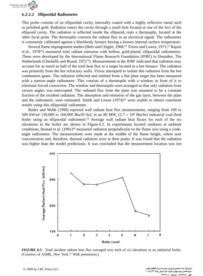
6.2.2.2 Ellipsoidal Radiometer
This probe consists of an ellipsoidal cavity, internally coated with a highly reflective metal such
as polished gold. Radiation enters the cavity through a small hole located at one of the foci of the ellipsoid cavity. The radiation is reflected inside the ellipsoid, onto a thermopile, located at the other focal point. The thermopile converts the radiant flux to an electrical signal. The radiometer is commonly calibrated against a blackbody furnace having a known internal surface temperature.
Several flame impingement studies (Beér and Chigier, 1968;32 Vizioz and Lowes, 1971;21 Rajani et al., 197825) measured total radiant emission with hollow, gold-plated, ellipsoidal radiometers. These were developed by the International Flame Research Foundation (IFRF) in IJmuiden, The Netherlands (Chedaille and Braud, 197275). Measurements at the IFRF indicated that radiation may account for as much as half of the total heat flux to a target located in a hot furnace. The radiation was primarily from the hot refractory walls. Vizioz attempted to isolate this radiation from the hot combustion gases. The radiation reflected and emitted from a flat plate target has been measured with a narrow-angle radiometer. This consists of a thermopile with a window in front of it to eliminate forced convection. The window and thermopile were arranged so that only radiation from certain angles was intercepted. The radiated flux from the plate was assumed to be a constant fraction of the incident radiation. The absorption and emission of the gas layer, between the plate and the radiometer, were estimated. Smith and Lowes (1974)24 were unable to obtain consistent results using this ellipsoidal radiometer.
Butler and Webb (1990) reported wall radiant heat flux measurements, ranging from 100 to 500 kW/m2 (30,000 to 160,000 Btu/ft2-hr), in an 80 MWe (2.7 × 10⁸ Btu/hr) industrial coal-fired boiler using an ellipsoidal radiometer.76 Average wall radiant heat fluxes for each of the six elevations in the boiler are shown in Figure 6.5. In experiments located outdoors at ambient conditions, Hustad et al. (1991)66 measured radiation perpendicular to the flame axis using a wide-angle radiometer. The measurements were made at the middle of the flame height, where soot concentration and, therefore, thermal radiation were at their peaks. It was found that the radiation was higher than the model predictions. It was concluded that the measurement location was not
FIGURE 6.5 Total incident radiant heat flux averaged over each of six elevations in an industrial boiler. (Courtesy of ASME, New York.76 With permission.)
© 2000 by CRC Press LLC

representative of the entire flame. The calculated values were used instead of the actual measure-ments in subsequent analyses. Hustad (1992)68 found that radiation perpendicular to the flame axis
was 26%, 40%, and 44% of the total heat flux for CH4, C4H10, and C3H8, respectively at Ma = 1. For C3H8, at Ma = 0.6, radiation was 26% of the total flux. These results showed that luminous radiation may be important, even for gaseous fuels. Beltagui et al. (1993) used both a total heat flux probe and calorimetry to measure the total heat flux in a furnace and a radiometer to measure the radiant heat flux in the furnace.77 They studied the characteristics of swirling flames fired vertically into a water-cooled chamber 3 m (10 ft) long and 1 m (3 ft) i.d., divided into six sections for calorimetry. The firing rate was 400 kW (1.4 × 10⁶ Btu/hr) on natural gas, with equivalence ratios ranging from 0.70 to 1.35 and 5% excess air. The total heat flux probe measurements were in good agreement with the calorimetry calculations for each of the six sections. The radiation measurements showed that the radiant heat flux was at least half of the total flux and in some cases nearly accounted for all of the heat flux. The measurements also showed that the heat flux distribution was much more uniform for the case with no swirl and that the peak flux 70 kW/m2
(22,000 Btu/ft2-hr) which occurred in the second section downstream from the burner for the case with high swirl (S = 2.25), was almost double the peak flux 40 kW/m2 (13,000 Btu/ft2-hr) for the case without swirl.
Radiometers are generally of low cost and simple to use. They have good spatial resolution. They operate successfully at high temperatures. However, they must be calibrated. Ellipsoidal radiometers are difficult to use in very sooty or in particle-laden environments. That may foul the polished reflectors.
6.2.2.3 Spectral Radiometer
Baukal and Ji (1998) studied the spectral radiation from oxygen-enhanced flames.78 Spectral radiation was measured with a spectral radiometer from Monolight Instruments (now known as Macam Photometrics in Livingston, Scotland). Three scanning monochromator modules with appropriate sets of order-sorting filters were used to cover the spectral range from 0.25 µm to 5.0 µm. The spectral irradiance calibration was made with a quartz-tungsten-halogen lamp (Oriel Model 6333, Stratford, CT) in the 0.25 to 1.7 µm range, and with an IR emitter (Oriel Model 6580) in the 1.7 to 5.0 µm range. The results of this study were discussed in sections 3.3 and 4.2.1.4.
6.2.2.4 Other Techniques
In the Baukal and Ji (1998) study referred to above, spectral radiometers and the properties of molten glass were used to determine the optimal wavelength range for thermal radiation to penetrate into the glass.78 However, that method is time-consuming and expensive. A more convenient and reliable way to determine the penetrating radiation is desirable. While the scanning spectral radi-ometer employed in that work provides quantitative measurements of the penetrating radiation, it requires spectral irradiance calibration, is time-consuming, and may not be as conveniently applied to large-scale flames in industrial furnaces. A more convenient way is to use total radiometers with appropriate spectral filters. Total (heat flux) radiometers have a flat spectral response in the 0.6 to 15.0 µm region. Without any window or filter in front of it, a heat flux meter gives the integrated total radiation intensity over the entire 0.6 to 15.0 µm range. By using an appropriate spectral filter to block out the undesirable, longer wavelength (λ > 2.7 µm) radiation, a heat flux meter can then be used to conveniently give the integrated radiation intensity that would be most penetrating into molten glass. Ji and Baukal tested several optical filters and compared the results against a spectral radiometer. Among the filters tested, a Schott BK7 optical glass filter exhibited a sharp cutoff transmission at λ = 2.7 µm. It became opaque at longer wavelengths for filter thickness greater than 6 mm (0.25 in.). Figure 6.6 shows a comparison of the measured flame radiation spectrum after it has passed through a room-temperature BK7 glass window, and the calculated flame radiation
© 2000 by CRC Press LLC
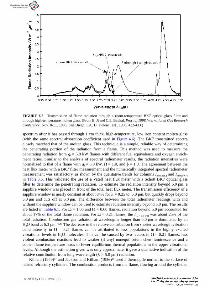
spectrum after it has passed through 1 cm thick, high-temperature, low iron content molten glass (with the same spectral absorption coefficient used in Figure 4.6). The BK7 transmitted spectra closely matched that of the molten glass. This technique is a simple, reliable way of determining the penetrating portion of the radiation from a flame. This method was used to measure the penetrating radiation from qf = 5.0 kW flames with different fuel equivalence and oxygen enrich-ment ratios. Similar to the analysis of spectral radiometer results, the radiation intensities were normalized to that of a flame with qf = 5.0 kW, Ω = 1.0, and φ = 1.0. The agreement between the heat flux meter with a BK7 filter measurement and the numerically integrated spectral radiometer measurement was satisfactory, as shown by the qualitative trends for columns Inrm(pen.) and Inrm(BK7)
in Table 3.5. This validated the use of a Vatell heat flux meter with a Schott BK7 optical glass filter to determine the penetrating radiation. To estimate the radiation intensity beyond 5.0 µm, a sapphire window was placed in front of the total heat flux meter. The transmission efficiency of a sapphire window is nearly constant at about 84% for λ = 0.25 to 5.0 µm, but quickly drops beyond 5.0 µm and cuts off at 6.0 µm. The difference between the total radiometer readings with and without the sapphire window can be used to estimate radiation intensity beyond 5.0 µm. The results are listed in Table 6.1. For Ω = 1.00 and Ω = 0.60 flames, radiation beyond 5.0 µm accounted for about 17% of the total flame radiation. For Ω = 0.21 flames, the I(λ > 5.0 µm) was about 25% of the total radiation. Combustion gas radiation at wavelengths longer than 5.0 µm is dominated by an H2O band at 6.3 µm.79,80 The decrease in the relative contribution from shorter wavelength vibration band intensity in Ω = 0.21 flames can be attributed to less populations in the highly excited vibrational levels in H2O molecules. This can be caused by two factors in Ω = 0.21 flames: less violent combustion reactions lead to weaker (if any) nonequilibrium chemiluminescence and a cooler flame temperature leads to fewer equilibrium thermal populations in the upper vibrational levels. Although the estimation given was only approximate, it gave a qualitative indication of the relative contribution from long-wavelength (λ > 5.0 µm) radiation.
Kilham (1949)17 and Jackson and Kilham (1956)18 used a thermopile normal to the surface of heated refractory cylinders. The combustion products from the flame, flowing around the cylinder,
FIGURE 6.6 Transmission of flame radiation through a room-temperature BK7 optical glass filter and through high-temperature molten glass. (From B. Ji and C.E. Baukal, Proc. of 1998 International Gas Research Conference, Nov. 8-11, 1998, San Diego, CA, D. Dolenc, Ed., 1998, 422-433.)
© 2000 by CRC Press LLC

TABLE 6.1
were also in the field of view. Therefore, the sum of the radiation from the gases — and from the cylinder surface — were measured. Two screens with narrow slit openings were placed between the flame and the detector to limit the field of view to a small region around the heated cylinder. Giedt et al. (1960)49 measured radiation for a H/H2 /CO mixture flame. From available data and radiation measurements, the gas emissivity was estimated to be 0.001. Nonluminous gas radiation was calculated to be, at most, only 2% of the total heat flux. Woodruff and Giedt (1966)50 measured gas and surface radiation, with two Leeds and Northrup mirror-type rayotubes. Radiation was found to be a negligible effect. Veldman et al. (1975)52 concluded that the measured radiation from an air/C3H8 flame was negligible. No details of the measurement techniques were given.
Baukal and Gebhart (1997) used surfaces of different emissivities to study flame radiation.81
As previously discussed in section 4.2.1.5.1, polished metal surfaces were used as the low-emissivity surfaces. Surfaces coated with a high-temperature flat black paint were used as the high-emissivity surfaces. One of the problems with the polished surfaces was very rapid degradation of both the brass and copper surfaces. Within minutes, those surfaces lost much of their reflectivity, due to the contact with the flame gases. The polished stainless steel surfaces remained reflective for over an hour. There was no noticeable degradation of the blackened surfaces for all three target materials after hours of operation.
Sivathanu et al. (1990) measured the soot volume fractions in highly turbulent and strongly radiating flames, which are common industrial-type flames.82 They used laser extinction measure-ments made with a three-line optical probe which had laser extinction at 632 nm and two-wavelength emission pyrometry at 900 and 1000 nm.
6.2.3 CONVECTIVE HEAT FLUX
In low-temperature processes, radiation may be insignificant and can be ignored, which means that the convective heat flux can be measured with a standard heat flux gage. However, in high-temperature combustion processes where radiation is very significant, it is difficult to directly measure the convective heat flux. The technique commonly used is to measure the total heat flux and the radiant flux and then to calculate the convective heat flux by subtracting the two. This obviously works only if there are no other modes of heat transfer that contribute to the total heat flux. A related method to determine the convective heat flux is by using other measurements along with a calculation. To do this, the temperatures of the surface where the convection is occurring
Estimation of the Radiation Intensity Beyond 5.0 µm
Ω φ I(w/sap.) I(λ < 5.0 µm) I(w/o) I(λ > 5.0 µm) (λ >5.0 µm)%
1.00 0.67 0.0476 0.0567 0.0672 0.0105 161.00 0.80 0.0504 0.0600 0.0723 0.0123 171.00 1.00 0.0532 0.0633 0.0751 0.0118 161.00 1.33 0.0504 0.0600 0.0727 0.0127 171.00 1.50 0.0482 0.0574 0.0684 0.0110 161.00 1.60 0.0465 0.0554 0.0674 0.0120 181.00 1.79 0.0439 0.0523 0.0636 0.0113 181.00 1.89 0.0429 0.0511 0.0609 0.0098 161.00 2.00 0.0443 0.0527 0.0620 0.0093 150.60 1.00 0.0434 0.0517 0.0631 0.0114 180.21 1.00 0.0170 0.0202 0.0269 0.0067 25
Source: From B. Ji and C.E. Baukal, Proc. of 1998 International Gas Research
Conference, Nov. 8-11, 1998, San Diego, CA, D. Dolenc, Ed., 5, 422-433, 1998.
© 2000 by CRC Press LLC

and of the gas flowing over the surface, along with the gas velocity, are needed. Using the appropriate forced convection heat transfer equation for the given geometry, the convective heat flux can be
calculated. This method is useful as a check against other methods that may be used.
Another method of determining the convective heat flux by direct measurement involves adding a radiant shield between the heat source and the heat flux gage to exclude radiation from being received by the gage. The problem is that the shield often disturbs the flow and the measured flux is not representative of the actual convective flow. Another problem is that the surface temperature under the shield will be lower than it would be without the shield, so the measurement would need to be done quickly before the wall temperature under the shield drops too much. In addition, although radiation from the primary source (burners) may be shielded, the rest of the furnace walls may still contribute radiation to the gage.
A third technique that could be used is to make a perfectly reflective heat flux gage so that any radiation received by the gage is reflected away and not measured by the gage. Then, in theory, the gage would only measure convection, assuming no other heat transfer mechanisms were important. Although in theory this sounds plausible, the reality is that it is very difficult to have a perfect reflector in an industrial combustion environment.
A fourth technique that could be used is to use a heat flux gage embedded in the wall where convection is to be measured and then to turn off the radiant source and quickly take measurements with the gage. The radiation from the hot furnace walls can be calculated and subtracted from the total flux. Again, this method suffers from problems similar to the other methods above in that it relies on a transient condition and accurate calculations.
6.3 TEMPERATURE
Many different types of devices are used to measure temperature, depending on the temperature range and specific application. The most common device is the thermocouple.
6.3.1 GAS TEMPERATURE
The gas temperature is not needed if only the heat flux is to be determined. However, it is an important parameter for comparing the measured heat flux to analytical formulations and to determine the gas properties. Also, the temperature profile across the jet gives an indication of the flow uniformity, and of the entrainment rate of ambient air into the flame.
Several techniques have been used for measuring the spatial gas temperature distribution, including thermocouples and the various optical methods, such as Rayleigh and Raman scattering.2-5
At this time, the light scattering methods are very expensive and difficult to use (Heitor and Moreira, 1992).83 Their primary use is in turbulent flows, and where probe survivability is a problem. Thermocouples are preferable because of their well-established properties, low cost, and ease of use. Some optical techniques, such as line reversal, may be difficult to use because of the need to seed the flame with particles. Those seeds could plug burners with small passage sizes.
6.3.1.1 Suction Pyrometer
At the desired measurement location, gases are extracted from the flame through a sampling tube. A thermocouple is positioned just inside this tube, typically made of a ceramic or high temperature metal, which acts as a radiation shield. Examples of suction pyrometers are shown in Figure 6.7. This technique is particularly useful when measuring gas temperatures in hot-surfaced enclosures. Surface radiation from the walls to an unshielded thermocouple may introduce large errors in the gas temperature measurement. Chedaille and Braud (1972)75 and Goldman (1987)84 specifically discussed the use of a suction pyrometer to measure gas temperatures in combustors. This device has been successfully used to measure gas temperatures in excess of 2200K (3500°F). In flame
© 2000 by CRC Press LLC

(c)
FI and (c) in the roof of a furnace. (Courtesy of John Zink Co. LLC, Tulsa, OK
©
(a) (b)
GURE 6.7 Examples of suction pyrometers: (a) new, (b) in the sidewall of a furnace,. With permission.)
2000 by CRC Press LLC
impingement studies, Beér and Chigier (1968),32 Vizioz and Lowes (1971),21 Smith and Lowes (1974),24 and Rajani et al. (1978)25 measured gas temperatures with a suction pyrometer.
Grey (1965)85 described a technique related to suction pyrometry known as a twin sonic orifice
probe. In this technique, the gases were extracted at very high velocity, through two converging-diverging nozzles inside the probe. One limitation of the suction pyrometer is that active chemical reactions may also occur inside the probe passages for highly dissociated gases. With proper corrections, this effect may be overcome by the dual sonic orifice probe. Rajani25 and Ivernel and Vernotte (1979)63 used a twin sonic orifice probe to measure gas temperatures in oxygen/fuel flames up to 3060K and 2800K (5050°F and 4600°F), respectively.
6.3.1.2 Optical Techniques
Laurendeau (1987) has given a brief review of temperature measurements using light scattering techniques.86 The techniques discussed included spontaneous vibrational and rotational Raman scattering, Rayleigh scattering, and laser-induced fluorescence. Fluorescence methods were recom-mended for temporally resolved planar thermometry.
Chao and Goulard (1974) presented a nonlinear iterative inversion technique for calculating flame temperatures from a single-line-of-sight multifrequency set of radiance measurements.87
Kondic (1974) developed a method to measure the density and temperature fields in fluids along a light path where the light source and detector were located external to the system.88 Although a laser is the preferred light source, a conventional light source can also be used. The gas temperature is related to the density field and the index of refraction of the fluid. Hofmann and Leipertz (1996) presented experimental measurements of the temperature field in a sooting, methane/air flame using a new technique referred to as filtered Rayleigh scattering (FRS).89
Posillico (1986)23 made detailed spatial gas temperature measurements using Raman spectros-copy (Eckbreth, 19884), for air/CH4 flames impinging on a water-cooled flat plate. The highest reported gas temperature was 3200K (5300°F), although the adiabatic flame temperature for a stoichiometric air/CH4 flame is 2223K (3542°F). No explanation was given for this apparent discrepancy. Hughes et al. (1995) compared a suction pyrometer and CARS in an industrial-scale flame.90 Rumminger et al. (1996) have used laser-induced fluorescence (LIF) to measure gas temperatures at the exit of porous radiant burners.91 The measurements were slightly higher than those made with a thermocouple after all corrections had been made to both techniques. The overall uncertainty in the LIF measurements was estimated to be ±110°F (60K). Char and Yeh (1996) described an optical technique of measuring the flame temperature using a combination of mea-suring the infrared radiation at a selected wavelength (4.3 µm, which has the highest intensity for CO2 and H2O) and making some iterative calculations to determine the flame emissivity.92 The measurements were made on a fuel-lean (φ = 0.51) open propane flame. The results compared favorably with thermocouple measurements. A correlation was developed for the gas emissivity for this flame as a function of the gas temperature position from the burner outlet.
6.3.1.3 Fine Wire Thermocouples
Gas temperature is an important parameter to the extent that it affects the gas properties, which are temperature dependent. Most of the heat transfer equations for heat flux also contain the gas temperature explicitly, as part of the driving potential for heat transfer. A number of thermocouple alloys are available, depending on the temperature range and type of atmosphere (inert, vacuum, oxidizing, or reducing), as shown in Table 6.2.
In one flame impingement study, two types of thermocouples were used to measure the gas temperatures.93 For the low-temperature flames, uncoated bare wire Type B thermocouples (Pt-60% Rh/Pt-6% Rh) were used. The probes were designed according to the method recommended by Peterson (1981).94 However, those thermocouples melted at Ω > 0.25. For higher temperature
© 2000 by CRC Press LLC

TABLE 6.2
flames, an Ir/60% Ir-40% Rh thermocouple was used. Candler (1967)95 has referred to this ther-mocouple as a Type L. According to Blackburn and Caldwell (1964),96 this thermocouple can be used to measure temperatures up to 2400K (3900°F), within ± 20K ( ± 40°F), using the appropriate reference table. This accuracy only refers to the measured temperature. The actual gas temperature still requires correction for the losses from the thermocouple junction. The Type L thermocouple wires were 0.25 mm (0.01 in.) in diameter.
Heitor and Moreira (1992)83 provided an extensive review of the use of thermocouples in combustion environments. They stated that flow disturbances and measurement errors can be made negligible in laminar flows. They suggested a coating consisting of 90% Al2O3 and 10% MgO, which minimizes catalytic effects and is not toxic. According to Cookson et al. (1964),97 thermo-couple junctions should be coated. The junctions should also be as small as possible to prevent
Characteristics of Common Thermocouple Alloys.
Max T(°F)
Max T(°C)
AllowableAtmos. (Hot) Material Names
ANSITypea
ColorCode
Output(mv/100°F)
Accuracy (%)Sandarda Precisiona
5072 2800 Inert, H2, vacuum
Tungsten/tungsten 26% rhenium
— — 0.86 — —
5000 2760 Inert, H2, vacuum
Tungsten 5% rhenium/tungsten 26% rhenium
— — 0.76 — —
4000 2210 Inert, H2 Tungsten 3% rhenium/tungsten 35% rhenium
— — 0.74 — —
3720 1800 Oxidizingb Platinum 30% rhodium/platinum 6% rhodium
B — 0.43 1/2 1/4
2900 1600 Oxidizingb Platinum 13% rhodium/platinum
R — 0.64 1/4 1/4
2800 1540 Oxidizingb Platinum 10% rhodium/platinum
S — 0.57 1/4 1/4
2372 1300 Oxidizingb,c Platinel II (5355)/Platinel II (7674)
— — 2.20 5/8 —
2300 1260 Oxidizing Chromel/Alumel,d Tophel/Nial,e Advance T1/T2,f Thermo-Kanathal P/Ng
K Yellow red 2.20 4°F, or 3/4% 2°F, or 3/8%
1800 980 Reducinga Chromel/constantan E Purple red 4.20 1/2 3/81600 875 Reducing Iron/constantan J White red 3.00 4°F, or 3/4% 2°F, or 3/8%750 400 Reducing Copper/constantan T Blue red 2.50 3/4 3/8
a Per ANSI C96.1 Standard.b Avoid contact with carbon, hydrogen, metallic vapors, silica, reducing atmosphere.c @ Engelhard Corp.d @ Hoskins Mfg. Co.e Wilber B. Driver Co.f Driver-Harris Co.g The Kanthal Corp.
Source: From F. Kreith, Ed., CRC Handbook of Mechanical Engineering, CRC Press, Boca Raton, FL, 1998, 4-183.
© 2000 by CRC Press LLC

surface recombination effects (see section 4.1.1.2). Kent (1970)98 has listed the following general requirements for a proper thermocouple coating:
• Noncatalytic to the flame• Inert to the thermocouple material• Impermeable to gases to protect the thermocouple• Poor electrical conductor to prevent electrical shorts• Stable within the desired temperature range• Capable of being evenly applied
A coating made from a mixture of approximately 10% BeO/90%Y2O3 was recommended.When using thermocouples to measure high temperatures, the measurements must be corrected
for the errors due to radiation, convection, and wire conduction. Moffat (1998) noted the general equations for estimating these types of errors:99
(6.1)
(6.2)
(6.3)
where Econv = convection error, Erad = radiation error, Econd = conduction error, α = recovery factor, v = gas velocity, gc = universal gravitational constant, J = Joules constant, cp = gas specific heat, σ = Stefan-Boltzmann constant, ε = probe emissivity, h = convection coefficient for gas flowing over probe, Tprobe = absolute temperature of the probe, Tsurr = absolute temperature of the surround-ings, tgas = temperature of the gas flowing past the probe (usually what is being measured), tprobe mount = temperature of the probe mount, l = length of the exposed junction, Ac = area for convection heat transfer, k = probe thermal conductivity, and Acond = area for conduction heat transfer. Note that these are iterative calculations, as the temperature of the gas is the quantity being measured. Also, some of the quantities may be difficult to know with a high degree of precision. Some of these include the convection coefficient, the gas velocity, the probe emissivity, the mount temperature, and the exposed junction length. Therefore, there will still be some uncertainty even after the measurements have been corrected for these errors. In general, the errors increase as the probe size increases.
Several methods are commonly used to compensate for these errors. One is electrical compen-sation (Hayhurst and Kittelson, 1977).100 However, this method cannot be used at very high temperatures, where the thermocouple may already be near its melting point. Any additional heating may cause the thermocouple to fail. Another compensation method is to make measurements using diminishingly smaller diameter thermocouples (Bradley and Matthews, 1968101). The thermocouple measurements are plotted against the cross-sectional area of the thermocouple junction. The tem-perature curves are then extrapolated to a zero-diameter thermocouple. This eliminates the need for correcting the measurements for the losses from the junction. A third method is to compute the correction (Fristrom and Westenberg, 1965102). An energy balance at the thermocouple junction may be given as:
qcatalytic + qconduction + qradiation + qconvection = 0 (6.4)
Ev
g Jcc pconv = −( )1
2
2
α
Eh
T Trad probe surr= −( )σε 4 4
Et t
hA
kAc
condgas probe mount
cond
=−⎡
⎣⎢⎢
⎤
⎦⎥⎥
cosh 1
© 2000 by CRC Press LLC

Hayhurst and Kittelson (1977)100 have shown that only surface reactions contribute to catalytic heating. This is commonly neglected when the thermocouple is coated. Bradley and Matthews
(1968)101 have shown that conduction can be neglected for wires over approximately 1 mm (0.04 in.) long. When conduction effects can been neglected, the energy balance then simplifies to:
(6.5)
where tT/C is the uncorrected temperature as measured with the thermocouple, and tj is the corrected temperature. The radiation from the environment to the junction has been neglected. An emissivity of 0.14 was recommended for uncoated platinum Type B thermocouple (Sparrow and Cess, 1978103). An emissivity of 0.60 was recommended for a coated Type L thermocouple (Peterson and Lauren-deau, 1985104). The convection coefficient was calculated using the equation recommended by Hinze (1959):105
(6.6)
An iterative procedure is required to calculate tj because the gas properties used to calculate the convection coefficient are dependent on tj. The gas temperature tj may also be required to calculate the gas velocity when, for example, Pitot-static probe measurements are used to calculate the velocity. Son et al. (1986) presented a mathematical method to compensate for the thermal inertia effects of thermocouples.106 These effects can cause errors if not properly corrected.
Many researchers have used fine wire thermocouples (T/Cs), with and without coatings. Very fine thermocouples minimize the disturbance to the flow. Buhr et al. (1973)33 and Kremer et al. (1974)34 used electrical compensation for radiation and conduction heat losses. Horsley et al. (1982),64 Kataoka et al. (1984),39 You (1985),44 Hargrave et al. (1987a),107 and Hustad et al. (1991, 1992)66-68 calculated corrections for the heat losses from the thermocouple junction. In some studies, radiation losses were corrected using successively smaller diameter thermocouples. These mea-surements were extrapolated to a vanishingly small thermocouple junction diameter. This method was suggested by Nichols (1900)108 and was improved by Bradley and Matthews (1968).101 Costa et al. (1996) used a bare 300 µm diameter wire uncoated Pt/Pt13%Rh thermocouple to measure gas temperatures inside an industrial glass-melting furnace.109 Mital et al. (1996) used three different diameter (76, 125, and 200 µm) fine wire, Type R thermocouples to measure the gas temperature inside porous ceramic radiant burners.110
Most high-temperature applications require some type of protective coating on the thermocouple unless the atmosphere is inert. Kaskan (1957)111 described a procedure for applying a silica coating to thermocouples. The junction was immersed in a flame containing a small amount of hexamethyl-disiloxane. This produced a uniform coating of fused quartz. It was found that the coating failed at about 1900K (3000°F), due to softening of the silica. Cookson and Kilham (1963),29 Kilham and Dunham (1967),30 and Milson and Chigier (1973)51 used silica coatings to prevent catalyic hydrogen atom recombination on the platinum in the thermocouple (Fristrom and Westenberg, 1965102). Madson and Theby (1984)112 showed that uncoated platinum alloy thermocouples signif-icantly overpredicted temperature, compared to silica-coated thermocouples in an O2 /Ar/CH4 flame. Pollock (1984)113 has shown that silica coatings may contaminate platinum-alloy thermocouple wires in chemically reducing environments. Kremer et al. (1974)34 used Al2O3 to prevent radical recombination. Hoogendoorn et al. (1978),35 Popiel et al. (1980),36 and Van der Meer (1991)46 used a yttrium/beryllium oxide (Yt2O3/BeO), as recommended by Kent (1970).98 This eliminates silica contamination. Unfortunately, beryllia is toxic and extremely poisonous.
Rumminger et al. (1996) used fine wire thermocouples to measure the gas temperature above the surface of a porous radiant burner.91 At 5 mm (0.2 in.) above the surface, they estimated a temperature correction of 270K (490°F), including the effects of re-radiation from the burner surface
t t t hj = +T C T C T Cσε 4
Nu = +0 42 0 570 2 0 33 0 5. Pr . Pr Re. . .
© 2000 by CRC Press LLC

to the thermocouple bead. Such a large correction resulted from a relatively large bead size (460 µm), high bead emissivity (0.6), and relatively slow gas flow (Red 0.9, Nu 0.7).
Fine wire thermocouples are of low cost and easy to use. They have short response times and
good spacial resolution. However, they are somewhat intrusive to the flame. Corrections are also required due to heat transfer effects at the junction bead. These include radiation from the bead to the environment and the heat conduction along the thermocouple wires. Often, the junction must be coated to prevent catalytic reactions. There are also material limitations, due to high-temperature oxidizing and reducing conditions.
6.3.1.4 Line Reversal
Many researchers have used this technique, originally suggested by Féry (1903),114 to measure flame temperatures. The flame is commonly seeded with sodium salt. The salt vaporizes in the flame and dissociates into sodium atoms and other products. These excited atoms emit at a specific wavelength. This radiation is then compared to a calibrated reference source, such as a tungsten filament lamp. The temperature of this source is adjusted until it matches the seed radiation. To the naked eye, the background source appears to disappear when it is at the same temperature as the flame. Strong et al. (1949) have given a general discussion of this technique to measure the temperatures in flames.115
Kilham (1949)17 used a spectrometer to compare the flame with the filament. Fells and Harker (1968)20 estimated the accuracy of their measurements to be 20K. Nawaz (1973)58 and Fairweather et al. (1984)59,60 introduced sodium chloride smoke, by passing N2 over molten salt, through a tube in the center of the burner. Therefore, only the temperatures along the central axis of the flame were measured. This reduced the influence of ambient air entrainment cooling effects at the flame periphery. Nawaz used a high-pressure xenon arc lamp (maximum temperature of 5000K, or 8500°F) as the comparison radiator, since the temperature levels were out of the range of the conventional tungsten lamps that were available at that time. Measured temperatures were 50K to 100K (90°F to 180°F) below the calculated adiabatic flame temperature. Fairweather (1984)60
measured a 33K (59°F) and 40K (72°F) reduction, across the equilibrium zone between the reaction zone and the stagnation point, for laminar and turbulent flames, respectively. Atmospheric air entrainment into the flame was thought to be a possible explanation for this effect.
This method is only slightly intrusive, due to the seeding. It is of relatively low cost. It may be effectively used for very high temperatures. However, the seeded field must be uniform. This may require the addition of a carrier gas to transport the seeds into the flame. Only an average gas temperature, across the flame, is measured. A calibrated reference light source is required.
6.3.2 SURFACE TEMPERATURE
There are two common ways to measure the surface temperature of an object, which are discussed next.
6.3.2.1 Embedded Thermocouple
In the flame impingement study by Baukal (1996), a Type K thermocouple was imbedded in the impingement rings of calorimeters.93 The thermocouples had an 0.5 mm (0.02 in.) o.d. inconel sheath, and the clearance hole in the side of each impingement ring was 0.64 mm (0.025 in.) i.d. A high-conductivity anti-seize sealant was applied to the end of each thermocouple before it was inserted into a ring to ensure good thermal contact. These thermocouples measured the temperatures at the middle of each impingement ring. The hot face temperatures were then calculated using the one-dimensional, steady-state conduction equation. Using the calculated heat flux to each ring, the hot face temperature, tw, was calculated using:
(6.7)t tq l
kw middle= + ′′ 1
1
2
© 2000 by CRC Press LLC

where tmiddle was the measured temperature at the middle of the ring, q″ was the calculated heat flux to the ring, l1 was the thickness of the impingement ring, and k1 was the thermal conductivity of the impingement ring. A typical result is shown in Figure 6.8. This graph shows that the wall temperatures decreased as the axial distance between the burner and the target decreased. However, for L > 2, the differences became smaller.
6.3.2.2 Infrared Detectors
Thermal imaging systems have been used for years in a variety of applications, including military and intelligence surveillance activities. Within about the last decade, the cost of these systems has declined enough that they are now being routinely used to measure temperatures in combustion applications. In combustion systems, these infrared imaging systems are typically used to measure the temperature of the furnace or heater walls, the heat load which might be a material like scrap metal or a tube used for process fluid heating, or the burner itself. Imaging systems are primarily used as a diagnostic to detect hot spots that could indicate potential problem areas.
Infrared detectors have a number of potential advantages over thermocouples:116
• Faster response times• Very high accuracies• Able to measure temperatures on moving objects• Able to measure higher temperatures than conventional thermocouples• Able to give two-dimensional temperature profiles• Do not disturb the surface being measured• Are not dependent on how they are attached to the surface, as thermocouples are, to get
an accurate surface temperature measurement
FIGURE 6.8 Surface temperature (tw) for O2 /natural gas flames (qf = 15.0 kW) impinging on an untreated stainless surface. (From C.E. Baukal, Heat Transfer from Flame Impingement Normal to a Plane Surface, Ph.D. thesis, University of Pennsylvania, 1996.)
© 2000 by CRC Press LLC
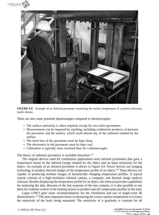
There are also some potential disadvantages compared to thermocouples:
• The surface emissivity is often required, except for two-color pyrometers.• Measurements can be impaired by anything, including combustion products, in between
the pyrometer and the surface, which could absorb any of the radiation emitted by the surface.
• The front lens of the pyrometer must be kept clean.• The electronics in the pyrometer must be kept cool.• Calibration is typically more involved than for a thermocouple.
The theory of radiation pyrometry is available elsewhere.117
The original devices used for combustion applications were infrared pyrometers that gave a temperature based on the infrared energy emitted by the object and an input emissivity for the object. An example of an infrared pyrometer is shown in Figure 6.9. Newer devices use imaging technology to produce thermal images of the temperature profile of an object.118 These devices are capable of producing realtime images of dynamically changing temperature profiles. A typical system consists of a high-resolution infrared camera, a computer, and thermal image analysis software. Besides displaying the temperature profile for an object, the software provides capabilities for analyzing the data. Because of the fast response of the new systems, it is also possible to use them for realtime control of the heating system to produce specific temperature profiles in the load.
Lappe (1997) gave some recommendations for the installation and use of single-color IR thermometers.119 The most important factor in measuring the correct surface temperature is to know the emissivity of the body being measured. The emissivity of a graybody is constant for all
FIGURE 6.9 Example of an infrared pyrometer measuring the surface temperature of a porous refractory matrix burner.
© 2000 by CRC Press LLC

wavelengths and usually does not change significantly with temperature unless there is a change in the material or in its surface characteristics. For example, if a solid material melts and becomes
liquid, there may be a significant change in its emissivity. Another example is if a metal oxidizes or becomes roughened from wear, its emissivity also may change dramatically. Lappe recommended using the shortest wavelength instrument possible to measure the surface temperature for two reasons. The first is that the difference in the emissivity of common surfaces such as metals is usually significantly less at shorter wavelengths, with the difference increasing with wavelength. Therefore, there will be less error if the emissivity used on the pyrometer is not properly adjusted for changes in the surface conditions of the body whose temperature is being measured. The second reason is that lower wavelength instruments typically have less error in the temperature reading compared to higher wavelength units. Lappe also gave some recommendations for the installation of these units:
• Ensure that the unit is focused properly on the object of interest and that the spot size is the correct size.
• Ensure that there are no obstructions (e.g., sightports walls, smoke, steam, etc.) between the pyrometer and the surface being measured.
• Fiber optic systems may be appropriate for certain applications.• Ensure that the interconnecting cable is not overheated or installed with other wires that
may carry high voltages that could adversely affect the signal.• Ensure that the sensing head is kept clean and cool, but not overcooled which could
cause condensation in the unit.• Keep the lens clean with a purge of clean dry air.• Have the instrument calibrated at least annually.
Two-color pyrometers avoid the problem of determining the emissivity of the surface.
6.4 GAS FLOW
6.4.1 GAS VELOCITY
The gas velocity of impinging flame jets is not required if only the measured heat flux is of interest. However, the velocity is very important for comparing the measured flux data to analytic models. Also, the velocity profile indicates whether or not the jet is fully developed before it impacts on the target. The two most common techniques for measuring velocity have been Pitot tubes and laser Doppler velocimeters (LDV). Some other techniques are also considered below.
6.4.1.1 Pitot Tubes
Pitot tubes and Prandtl probes are used to measure the total and static pressures, respectively, in a flow. Both sensors are tubes. One end is exposed to the flow and the other end is connected to a pressure transducer. The Pitot tube has a hole at the end of the tube. It is aligned in the main flow direction to measure total head pressure. The Prandtl probe has a hole on the side of the tube. The sensor tube is aligned parallel to the main flow direction to measure the static pressure. The difference between the total and static pressures (i.e., the dynamic pressure) is proportional to the square root of the gas velocity. In flames, these pressures are low but are measurable (Lewis et al., 1956).120 The two probes may be combined together, as a Pitot-static probe. The Pitot tube and combined Pitot-static probe are shown in Figure 6.10.121 The combined probe is sometimes referred
© 2000 by CRC Press LLC

to as simply a Pitot tube. Some studies have not distinguished between a true Pitot tube and a Pitot-static tube. In some studies, the static pressure at the probe location was assumed to be the same as the ambient. Single-hole Pitot tubes only measure the velocity component parallel to the probe. In addition to velocity, specially designed five-hole Pitot tubes may also indicate the gas flow direction. See Reference 9 for a discussion of both one- and five-hole Pitot tubes, including their use in combustion applications. Becker9 showed the importance of the probe tip shape, although this feature has rarely been described in the studies considered here.
The equation governing the response of a Pitot probe is commonly given as (Becker and Brown, 1974):122
(6.8)
where pt is the total or impact pressure, pst is the static pressure, and Cp is the probe calibration constant. Becker and Brown studied the response of Pitot probes in turbulent nonreacting gas streams. The following terminology is used to specify the recommendations of that study:
d1 = Total pressure hole i.d.d2 = Probe o.d.d3 = Static pressure hole i.d.l1 = Internal length before any change in diameter or direction of total impact tubel2 = External length before any change in diameter or direction of probel3 = Length from probe tip to centerline of static pressure hole
In that study, the following conditions were assumed:
1. The probe is long enough (l2/d2 > 6) so that the downstream geometry has a negligible effect on the response.
2. The internal geometry (l1/d1 > 3) has a negligible effect on the response.3. Compressibility effects are small (Ma < 0.3).
A hemispherically nosed, water-cooled P-S probe was used by Baukal (1996).93 It had the following dimensions: d1 = d3 = 1.40 mm (0.055 in.); d2 = 12.7 mm (0.5 in.); l1 = l2 = 14.6 cm (5.75 in.); l3 = 22.2 mm (0.875 in.). These dimensions satisfied conditions 1 and 2 above. The low gas flow rates
FIGURE 6.10 Flow measurement using (a) Pitot tube and (b) Pitot-static tube. (Adapted from C. Swan, in International Encyclopedia of Heat & Mass Transfer, G.F. Hewitt, G.L. Shires, and Y.V. Polezhaev, Eds., CRC Press, Boca Raton, FL, 1997, 842.)
v p p C= −( )2 t st pρ
© 2000 by CRC Press LLC
satisfied condition 3. The probe had a single static pressure inlet, as recommended by Cho and Becker (1985).123
For a hemi-nosed probe geometry, Chue (1975)124 recommended that ReP > 1000, so that Cp Ý 1,
and no calibration would be required. Becker (1993)9 recommended ReP > 600 to avoid calibration. Becker and Brown (1974)122 recommended d1/d2 < 0.3, with 0.12 as the optimum. Chue (1975)124
recommended d3/d2 = 0.01 to 0.50. Cho and Becker (1985)123 recommended d3/d2 < 0.25, and preferably < 0.1. Cho and Becker (1985)123 recommended l3/d2 = 2.
The above methods are simple and of relatively low cost. However, they are intrusive to the flow. They usually require cooling in combustion environments. This technique has a very limited ability to detect turbulent fluctuations. It also requires careful use in highly recirculating flows.
There are many potential sources of errors when using Pitot tubes, including:125
• Errors in the pressure gages• Misalignment of the Pitot tube• Wall interference for measurements close to a surface• Instrument vibrations• Flaws in the nose of the probe• Location in recirculation or shear zones• Viscous effects in low-flow, highly viscous flows or for extremely small tubes
Therefore, care must be used when using P-S probes.
6.4.1.2 Laser Doppler Velocimeter
Laser Doppler velocimetry (LDV) is an optical technique for measuring fluid velocities. For a given velocity direction, two laser beams must cross to create a small scattering volume. As a particle passes through that volume, a Doppler shift is produced. This is detected by receiving optics. With proper processing, the velocity can be calculated from this signal. Baker et al. (1972) presented LDV measurements made on town gas and methane flames from an industrial burner.126 Chigier (1989),127 Most (1991),128 and Heitor et al. (1992)129 discussed the use of LDVs in combusting flows. Fingerson and Menon (1998) discussed this technique in some detail, although not specifi-cally for combustion measurements.130
For air/natural gas flames impinging on a flat plate, Hoogendoorn et al. (1978)35 and Popiel et al. (1980)36 used an LDV in turbulent and laminar flames, respectively. The LDV measured turbulent fluctuations. Pitot tubes were used to measure mean velocities. Hoogendoorn (1978),35
Popiel (1980),36 and van der Meer (1991)46 used MgO seeds of unspecified diameter. You (1985)44
used oil droplets and a small acetylene sooting flame to generate additional particles in the regions of their flames that had inadequate soot particle concentrations for LDV measurements. The mean particle diameter was 0.6 µm. Fairweather et al. (1984)60 used 1 µm mean diameter alumina particles for seeding. A near-uniform free stream velocity was measured in the equilibrium zone of their laminar air/CH4 flames. In their turbulent flames, there was a 2% and 40% increase in the free stream velocity and in the turbulent intensity, respectively. Hargrave et al. (1984, 1987),37,107 used an LDV to measure velocities and turbulent intensities in turbulent flames. The flames were seeded with alumina particles. The mean size was 1 µm, with a maximum size of 2 µm. Posillico (1986)23
used an LDV, with Al2O3 seeds of unspecified size. Van der Meer’s (1987)131 measured velocity profile was not uniform, as stated by others (e.g., see Reference 35) for tunnel burners. Van der Meer (1991)46 used an LDV to determine the stagnation velocity gradient (discussed in the next section), the velocity field, and the turbulence level. The turbulence level increased with L up to about L = 5, where it flattened out. This behavior was seen even in initially laminar flames.
This technique has excellent temporal resolution; it can be used to measure turbulence, is less intrusive to the flow field than Pitot tubes, and can be used very close to walls without affecting the flow field. An LDV system can also measure multidimensional velocity fields, even in recirculating
© 2000 by CRC Press LLC

flows. New fiber-optic techniques make optical alignment easier than before. However, an LDV system is expensive. Flames from gaseous fuels commonly require seeding to ensure sufficient
scattering. The choice of seeds is limited in high-temperature oxidizing environments. Optical refraction may occur in regions of large density and temperature gradients in the flame. This may reduce the signal strength and resolution.
6.4.1.3 Other Techniques
Kilham (1949),17 Jackson and Kilham (1956),18 and Kilham and Purvis (1971, 1978)57,62 used shadowgraph photography to estimate the flame cross-sectional area. This data was then used to calculate an average gas velocity, based on the known gas flow rate and the measured temperature. Anderson and Stresino (1963)26 estimated the gas velocity, based on the measured thrust of a flame impinging on a flat surface. The velocity was calculated in terms of gas dynamic considerations, based on the known flow rates and the estimated gas densities. Reed (1963)27 calculated the average gas velocity using the gas flow rates, the estimated flame diameter, and the adiabatic flame temperature. Conolly (1971)132 used a particle tracking photography method. Results agreed well with Pitot tube measurements. Nawaz (1973)58 calculated the average gas velocity in the same manner as Reed. However, the measured — instead of the adiabatic — flame temperature was used. Fairweather et al. (1984)59 concluded that the velocity profile for their tunnel burner was very uniform at any location downstream of the reaction zone, based on Pitot tube measurements. This justified using an estimated flame diameter, determined from photographic techniques, to calculate the gas velocity.
6.4.2 STATIC PRESSURE DISTRIBUTION
In many common flow geometries, such as free jets, the static pressure is assumed uniform and constant. However, in impinging jet flows, the static pressure in the stagnation region is often much higher than elsewhere in the flow. This is due to rapid deceleration and deflection of the impinging jet. The actual static pressure distribution has been measured near the stagnation point for two reasons. The first is to determine the velocity gradient adjacent to the surface, βs. The second is to determine the extent of the stagnation region.
6.4.2.1 Stagnation Velocity Gradient
This is an important parameter in the semianalytical solutions for the heat transfer from high-temperature gases impinging on a blunt-nosed body. These solutions are discussed in Chapter 7. An example is the solution by Sibulkin (1952),133 given in Equation 7.15. The stagnation velocity gradient has been defined as:
(6.9)
where the local velocity gradient is evaluated at the edge of the boundary layer (z = δ) along the axis of symmetry. A detailed discussion of this parameter is given by van der Meer (1987).131
Two different methods have been used to experimentally determine βs. The first involves measuring the static pressure distribution near the stagnation point. It can be shown (see Purvis, 1974134 or Tariq, 1982135) that:
βδ
sz r
vr
= ∂∂
⎛⎝⎜
⎞⎠⎟ = =, 0
© 2000 by CRC Press LLC

(6.10)βsstd p p r
=− ( ) ⎛
⎜⎞⎟
2
This is estimated by calculating the tangent to the graph of as a function of r at r = 0. Kilham and Purvis (1978)62 used 0.88 mm (0.035 in.) i.d. stainless steel tubes. These were mounted within a given radius, surrounding the stagnation point, in a large flat water-cooled copper plate. Using this array of static pressure measurements, they calculated the following relationship using Equation 6.10:
βs = ve /dj (6.11)
Rajani et al. (1978)25 and Popiel et al. (1980)36 measured βs at the stagnation surface, with small holes drilled into a flat plate target. Popiel used a 0.5 mm (0.02 in.) i.d. hole and determined the following relation:
βs = 9.7 ve /(x + dn) (6.12)
βs can also be experimentally determined from LDV measurements. By measuring the velocity distribution near the stagnation point, the gradient in Equation 6.10 can be directly computed. Van der Meer (1991)46 determined βs, for air/natural gas flames impinging on a cooled flat plate. The nondimensionalized velocity gradient was given as:
Bs = βs dn/vn (6.13)
This increased with L, to a peak at about L = 3. Thereafter, it decreased monotonically. For 1700 ð Ren ð 4250, Bs showed no dependence on Ren.
6.4.2.2 Stagnation Zone
The static pressure distribution around the impingement surface is also used to determine the extent of the stagnation zone. This zone is defined as the region where the static pressure, pst, exceeds the distant ambient pressure. The stagnation zone boundary is important in analyzing the mecha-nisms of the impinging jet process. The flow between the nozzle and the beginning of the stagnation zone, in the direction normal to the target, is a free jet. The boundary of the stagnation zone parallel to the target defines the start of the so-called wall region. This is a boundary layer flow. Both the free jet and the wall regions (see Figure 3.1) can be analyzed by well-established analysis.
Buhr (1969)136 measured the pst distribution in the radial direction, using a 0.75 mm (0.03 in.) i.d. Pitot tube. It was mounted flush with the surface of a water-cooled plane target. For the fuel-rich turbulent air/CH4 flame, L ranged from 13 to 53 with Ren = 19,680. Vizioz and Lowes (1971)21
measured the pst distribution along the radial direction of a plane surface. Holes of unspecified diameter were drilled through a water-cooled steel plate, for flames with and without swirl. The no-swirl flame showed a peak in pst, at R = 0 of nearly 100 Pa (0.0014 psig). The swirl flames showed peaks, at either R = 1.3 or 1.9, for pst between 70 and 80 Pa (0.010 and 0.012 psig), depending on the nozzle design. The stagnation zone appeared to extend to about R Ý 3.8. Vizioz also measured pst in the axial direction. The stagnation zone extended to Z = 2.3 to 4.0, depending on the test configuration. Kilham and Purvis (1978)62 and Horsley et al. (1982)64 used 0.88 mm (0.035 in.) i.d., while Hoogendoorn et al. (1978)35 used 0.5 mm (0.02 in.) i.d. stainless steel tubes, mounted within a given radius surrounding the stagnation point of a large flat water-cooled copper plate. Kilham found that the impingement region extended out to 2.2 < R < 2.7. The measurements were difficult, due to combustion product condensation obstructing the pressure taps.
ρr
dr⎝⎜ ⎠⎟ = 0
2 p p rst −( )( ) ρ
© 2000 by CRC Press LLC
6.5 GAS SPECIES
Gas composition is useful in determining combustion efficiency. For example, a gas sample at the
exit of a tunnel burner measures any fuel that has not been burned. A measurement of the gas composition near the target surface is useful in predicting the amount of thermochemical heat release from the radical species. This composition determines the level of species dissociation in the impinging jet.
Beér and Chigier (1968)32 measured gas compositions by extracting samples from the flame. Kremer et al. (1974)34 measured gas concentrations in the stagnation region. In both studies, the gases sampled were not specified and no data were reported. Conolly (1971)132 estimated the hydrogen atom concentration in flames. This was done by first comparing the spectral intensities of the radiation emitted from flames seeded with sodium and lithium at wavelengths of 589.0 and 670.8 nm, respectively. The composition was then estimated, assuming equilibrium conditions. These results showed super-equilibrium concentrations of H in a small region above the burner. Nawaz (1973)58 tried unsuccessfully to measure NO with a gas chromatograph (GC). The OH concentration was qualitatively determined — nonintrusively — by a line absorption method. The background source was a water discharge lamp. In general, CO2, H2O (calculated), N2, and O2
concentrations were higher than adiabatic equilibrium predictions. Also, CO and H2 concentrations were lower than predicted. Low probe quenching efficiency was suggested as causing CO and H2
to react with OH in the probe to produce CO2 and H2O, respectively. You (1985)44 extracted gas samples isokinetically through a 1 mm (0.04 in.) i.d. water-cooled stainless steel probe. Posillico (1986)23 used Raman spectroscopy (see Reference 4 for a discussion of this technique) to spatially measure CO2, N2, and O2 in an impinging air/CH4 flame. Hustad et al. (1991) measured O2
concentrations in pure diffusion flames to qualitatively determine air entrainment into the flames.66
Details of the technique were not given.There are several potential uncertainties with most of the extractive gas sampling techniques
that have been used. The most important one is subsequent chemical effects in the gas sampling system. Thereby, the measurements may not accurately reflect the actual gas composition at the sampling probe inlet. This makes it very difficult to accurately determine the trace radical species. On the other hand, these are of great interest in impingement flame studies. The sampling probe commonly must be cooled in combustion environments. This increases the size of the probe, making it more intrusive in the flame. This also adversely affects the spatial resolution of the measurements. Extractive gas sampling systems are unable to measure large gradients in composition. These gradients occur near the reaction zone. The residence time of the gases in the sampling system is much larger than the time scales characteristic of turbulent flames. Also, the gas chromatographs used in many of the studies commonly have a several minute delay time for the sample analysis. Therefore, only time-averaged measurements can be made.
6.6 OTHER MEASUREMENTS
A variety of other techniques have also been used in combustion studies. This chapter section is merely intended to give a sampling of those techniques and is in no way exhaustive or comprehensive, but is merely intended to be representative. Calcote and King (1955)137 used a Langmuir138 probe to study ionization in flames, which is important for calculating thermochemical heat release (see Chapter 4). Anderson and Stresino (1963)26 determined the flame diameter prior to impingement by an unspecified technique. Dunham (1963)139 attempted to use Schleiren photography (Reid, 1954)140
for visualization of a flame produced by a porous disk burner. Beér and Chigier (1968)32 measured soot concentration by an unspecified technique. Milson and Chigier (1973)51 photographed and filmed fuel-rich flames. The photographs showed distinct circulation eddy structures. The films showed the pulsating nature of the flow. Nawaz (1973)58 used photographs, projected on a screen, to estimate the flame diameters. Purvis (1974)134 used spark Schlieren photography. A capacitance
© 2000 by CRC Press LLC

discharge lamp produced a 0.2 µsec illumination time. Average flame lengths and widths were estimated. Veldman et al. (1975)52 used shadowgraph visualization (Reid, 1954).140 Rajani et al. (1978)25 used a Hubbard probe to determine flame boundaries. This probe is a combination of the two Prandtl probes discussed above. Two static pressure sampling points are located on opposite sides of the probe tip. The tip is aligned perpendicular to the flow direction, with the holes parallel to the burner axis. The stagnation points in the flow occur when there is zero pressure difference between the two holes. This separates the forward and reverse flows. Popiel et al. (1980)36 used the smoke wire technique to visualize large-scale eddies at about R = 1. These eddies were thought to be the reason why the peak heat flux was not at the stagnation point. You (1985)44 photographed flames in a darkened room, to determine the flame shape. Horsley et al. (1982)64 used Schlieren photography to study turbulence in industrial burners. Hargrave et al. (1987)107 also used Schlieren photography, with an argon spark-jet light source. It gave an illumination period of 0.2 µsec.
Snyder et al. (1989) used laser tomography to measure soot volume fractions in flames that are important in the analysis of luminous radiation from sooting flames.141 Turns et al. (1989) used a light scattering technique to visualize soot in turbulent diffusion flames.142 Using a light scattering technique, Hsu et al. (1990) measured the size and fume density of particles containing sodium and potassium that evolve from Kraft recovery furnaces in the combustion of black liquor produced in the production of paper products.143 Urban and Dryer (1990) used a light-scattering technique to measure the coke particle size distribution produced by the combustion of residual oil in an industrial boiler.144 Köylü and Faeth (1993) determined the structure of soot produced in buoyant laminar diffusion flames using a combination of thermophoretic sampling and transmission electron microscopy (TEM).145 Manickavasagam and Mengüç (1993) discussed transmission and scattering techniques using a CO2-laser nephelometer to measure radiative properties of coal/char particles on premixed ethylene-coal flames.146 Copin et al. (1998) used helium tracing to determine the residence time in an industrial furnace.147
FIGURE 6.11 Plexiglas model of a combustor. (Courtesy of John Zink Co. LLC, Tulsa, OK.)
© 2000 by CRC Press LLC

6.7 PHYSICAL MODELING
Before the advent of computers and computer modeling, a common method used to simulate a
process was physical modeling. This usually involves the construction of a small-scale model for use in studying some aspect of a combustor. One common technique has been to build a scale replica of a combustor or burner using a see-through material like plexiglas. An example of such a physical model is shown in Figure 6.11. Rather than having an actual flame, a substitute fluid (e.g., ambient-temperature gases [usually air] or water), would be used to study the fluid flow in the system. Neutral-buoyancy tracers would often be added to help in visualizing the flow through the system. Methods were devised to study pseudo heat transfer and chemical reactions using fluids that would either react with each other to produce a distinguishable product or fluids that would react with some type of treatment on the walls of the model to produce a reaction. Because all of these were done at ambient temperatures, they were very difficult to extrapolate to combustion conditions. However, they were useful for studying the fluid flow characteristics of the system.
These small-scale models were often time-consuming and expensive to build. They required the skill of a trained craftsman. They could only be used to reasonably study a few variables of importance in combustion processes, usually fluid flow and sometimes heat transfer and chemical reactions. However, they were not capable of properly simulating, for example, the radiation heat transfer in a high-temperature combustor. Another important limitation is that there may be signif-icant problems scaling-up the results to actual combustor conditions. Significant changes to the model can also be costly, which can make parameter studies expensive. Without some type of scaling correlations based on field data from full-scale systems, it is often difficult to convince end users to accept the results from these small-scale physical models. As a result of these disadvantages and the ready availability of computational fluid dynamic modeling, these small-scale physical models are not often used today.
Another type of physical model sometimes used, is a large-scale mock-up of a combustor and burner. An example is shown in Figure 6.12. These physical models can be full scale, but still do not have actual combustion. They can be used as wind tunnel simulators to study the fluid flow through a burner and a combustor. Measurements in these simulators are useful for calculating things like the pressure drop through a burner and for generating validation data for cold flow CFD models. This type of model is often much less expensive to build than an actual furnace because no insulation, water-cooling, complicated flow controls, gas analysis equipment, or associated safety equipment are required. However, except for the scale-up concerns, these models have similar limitations to the small-scale models discussed above. As a result, they are usually only used in limited circum-stances. The latest visualization techniques for CFD modeling now make it possible to create virtual combustors where — like the latest video games — one can travel through the combustion space and view any parameter of interest, including temperature, velocity, heat flux, or species concentra-tion. Although this capability is only in its infancy, as it becomes more affordable for the average combustion design engineer, there will be even less use for the physical models.
REFERENCES
1. C.I. Okoh and R.A. Brown, Combustion Experimentation Handbook, Gas Research Institute Report GRI-88/0143, Chicago, IL, 1988.
1a. J.M. Beér and N.A. Chigier, Combustion Aerodynamics, Applied Science Publishers, London, 1972.2. D.F.G. Durão, M.V. Heitor, J.H. Whitelaw, and P.O. Witze, Combusting Flow Diagnostics, Kluwer
Academic, Dordrecht, The Netherlands, 1992.3. A.M.K.P. Taylor, Instrumentation for Flows with Combustion, Academic Press, London, 1993.
3a. R.M. Fristrom, Flame Structure and Processes, Oxford University Press, New York, 1995.4. A.C. Eckbreth, Laser Diagnostics for Combustion Temperature and Species, Abacus Press, Cambridge,
MA, 1988.
© 2000 by CRC Press LLC

5. N. Chigier, Combustion Measurements, Hemisphere, New York, 1991.6. R.M. Fristrom, Probe measurements in laminar combustion systems, in Combustion Measurements —
Modern Techniques and Instrumentation, R. Goulard, Ed., Academic Press, New York, 1976.7. C.T. Bowman, Probe measurements in flames, Prog. Astr. Aero., 53, 1-24, 1977.8. F.C. Gouldin, Probe Measurements in multi-dimensional reacting flows, in Testing and Measurement
Techniques in Heat Transfer and Combustion, AGARD CP-281, Paper #4, 1980.9. H.A. Becker, Physical probes, in Instrumentation for Flows with Combustion, A.M.K.P. Taylor, Ed.,
Academic Press, London, 1993, 53-112.10. J. Newbold, M.C. McQuay, B.W. Webb, and A.M. Huber, The experimental characterization of the
combustion process in an industrial, gas-fired, flat-glass furnace, 29th Int. ISATA Conf. — Automotive Technology & Automation, Florence, Italy, June, Automotive Assoc. Ltd., 2, 967-976, 1996.
11. P.R. Solomon, P.E. Best, R.M. Carangelo, J.R. Markham, P.-L. Chien, R.J. Santoro, and H.G. Semer-jian, FT-IR emission/transmission spectroscopy for in situ combustion diagnostics, Twenty-First Sym-posium (International) on Combustion, The Combustion Institute, Pittsburgh, PA, 1986, 1763-1771.
12. A.C. Eckbreth, Recent advances in laser diagnostics for temperature and species concentrations in combustion, Eighteenth Symposium (International) on Combustion, The Combustion Institute, Pitts-burgh, PA, 1980, 1471-1488.
13. S.S. Penner, C.P. Wang, and M.Y. Bahadori, Laser diagnostics applied to combustion systems, Twentieth Symposium (International) on Combustion, The Combustion Institute, Pittsburgh, PA, 1984, 1149-1176.
14. R.K. Hanson, Combustion diagnostics: planar imaging techniques, Twenty-First Symposium (Interna-tional) on Combustion, The Combustion Institute, Pittsburgh, PA, 1986, 1677-1691.
15. N.R. Fornaciari, R.W. Schefer, P.M. Walsh, and L.E. Claytor, Application of laser-based diagnostics to industrial scale burners, Proc. of 1995 International Gas Research Conf., D.A. Dolenc, Ed., Govt. Institutes, Rockville, MD, 1996, 2398-2405.
16. M. Perrin, J. Imbach, S. Albert, J. Mariasine, and A. Quinqueneau, Application of advanced instanta-neous in-flame measurements techniques in an industrial flame with preheated air, Proc. of 1995 International Gas Research Conf., D.A. Dolenc, Ed., Govt. Institutes, Rockville, MD, 1996, 2406-2415.
FIGURE 6.12 Wind tunnel simulator for studying fluid flow in a combustor. (Courtesy of John Zink Co. LLC, Tulsa, OK.)
© 2000 by CRC Press LLC

17. J.K. Kilham, Energy transfer from flame gases to solids, Third Symposium on Combustion and Flame and Explosion Phenomena, The Williams and Wilkins Co., Baltimore, MD, 1949, 733-740.
18. E.G. Jackson and J.K. Kilham, Heat transfer from combustion products by forced convection, Ind.
Eng. Chem., 48(11), 2077-2079, 1956.19. R.M. Davies, Heat Transfer measurements on electrically-boosted flames. Tenth Symposium (Inter-
national) on Combustion, The Combustion Institute, Pittsburgh, PA, 1965, 755-766.20. I. Fells and J.H. Harker, An investigation into heat transfer from unseeded propane-air flames aug-
mented with D.C. electrical power. Comb. Flame, 12, 587-596, 1968.21. J.-P. Vizioz and T.M. Lowes, Convective Heat Transfer from Impinging Flame Jets, Int. Flame
Research Found. Report F 35/a/6, IJmuiden, The Netherlands, 1971.22. D.R. Davies, Heat Transfer from Working Flame Burners, B.S. thesis, Univ. of Salford, Salford, U.K.,
1979.23. C.J. Posillico, Raman Spectroscopic and LDV Measurements of a Methane Jet Impinging Normally
on a Flat Water-Cooled Boundary, Ph.D. thesis, Polytechnic Institute of New York, New York, 1986.24. R.B. Smith and T.M. Lowes, Convective heat transfer from impinging tunnel burner flames — A
short report on the NG-4 trials, Int. Flame Research Found. Report F 35/a/9, IJmuiden, The Nether-lands, 1974.
25. J.B. Rajani, R. Payne, and S. Michelfelder, Convective heat transfer from impinging oxygen-natural gas flames — Experimental results from the NG5 Trials, Int. Flame Research Found. Report F 35/a/12, IJmuiden, The Netherlands, 1978.
26. J.E. Anderson and E.F. Stresino, Heat transfer from flames impinging on flat and cylindrical surfaces, J. Heat Trans., 85(1), 49-54, 1963.
27. T.B. Reed, Heat-transfer intensity from induction plasma flames and oxy-hydrogen flames, J. Appl. Phys., 34(8), 2266-2269, 1963.
28. R.H. Fay, Heat transfer from fuel gas flames, Welding J. (Research Supplement), 380s-383s, 1967.29. R.A. Cookson and J.K. Kilham, Energy transfer from hydrogen-air flames, Ninth Symposium (Inter-
national) on Combustion, Academic Press, New York, 1963, 257-263.30. J.K. Kilham and P.G. Dunham, Energy transfer from carbon monoxide flames, Eleventh Symposium
(International) on Combustion, The Combustion Institute, Pittsburgh, PA, 1967, 899-905.31. R.A. Cookson, P.G. Dunham, and J.K. Kilham, Stagnation point heat flow meter, J. Sci. Instrum., 42,
260-262, 1965.32. J.M. Beér and N.A. Chigier, Impinging jet flames, Comb. Flame, 12, 575-586, 1968.33. E. Buhr, G. Haupt, and H. Kremer, Heat transfer from impinging turbulent jet flames to plane surfaces,
in Combustion Institute European Symposium 1973, F.J. Weinberg, Ed., Academic Press, New York, 1973, 607-612.
34. H. Kremer, E. Buhr, and R. Haupt, Heat transfer from turbulent free-jet flames to plane surfaces, in Heat Transfer in Flames, N.H. Afgan and J.M. Beér, Eds., Scripta Book Company, Washington, D.C., 1974, 463-472.
35. C.J. Hoogendoorn, C.O. Popiel, and T.H. van der Meer, Turbulent heat transfer on a plane surface in impingement round premixed flame jets, Proc. of 6th Int. Heat Trans. Conf., Toronto, 4, 107-112, 1978.
36. C.O. Popiel, T.H. van der Meer, and C.J. Hoogendoorn, Convective heat transfer on a plate in an impinging round hot gas jet of low Reynolds number, Int. J. Heat Mass Trans., 23, 1055-1068, 1980.
37. G.K. Hargrave and J.K. Kilham, The effect of turbulence intensity on convective heat transfer from premixed methane-air flames, Inst. Chem. Eng. Symp. Ser., 2(86), 1025-1034, 1984.
38. G.K. Hargrave, M. Fairweather, and J.K. Kilham, Forced convective heat transfer from premixed flames. 2. Impingement heat transfer, Int. J. Heat Fluid Flow, 8(2), 132-138, 1987.
39. K. Kataoka, H. Shundoh, and H. Matsuo, Convective heat transfer between a flat plate and a jet of hot gas impinging on it, in Drying ’84, A.S. Mujumdar, Ed., Hemisphere/Springer-Verlag, New York, 1984, 218-227.
40. J. Cassiano, M.V. Heitor and T.F. Silva, Combustion tests on an industrial glass-melting furnace, Fuel, 73(10), 1638-1642, 1994.
41. S.N. Shorin and V.A. Pechurkin, Effectivnost’ teploperenosa na poverkhnost’ plity ot vysokotemper-aturnoi strui produktov sjoraniya razlichnykh gazov (The effectiveness of heat transfer to the surface of a plate from a high-temperature jet of combustion products of various gases), Teoriya i Praktika Szhiganiya Gaza, 4, 134-143, 1968.
© 2000 by CRC Press LLC

42. E.M. Schulte and R.F. Kohl, A transducer for measuring high heat transfer rates, Rev. Sci. Instrum., 41(12), 1732-1740, 1970.
43. E.M. Schulte, Impingement heat transfer rates from torch flames, J. Heat Trans., 94, 231-233, 1972.44. H.-Z. You, An investigation of fire-plume impingement on a horizontal ceiling: 2. Impingement and
ceiling-jet regions, Fire & Materials, 9(l), 46-56, 1985.45. R. Gardon, A transducer for the measurement of heat flow rate, J. Heat Trans., 82, 396-398, 1960.46. T.H. Van der Meer, Stagnation point heat transfer from turbulent low Reynolds number jets and flame
jets, Exper. Ther. Fluid Sci., 4, 115-126, 1991.47. A. Barnes, Heat Flux Sensors. 2. Applications, Sensors, 16(2), 54-57, 1999.48. B. Gebhart, Heat Transfer, McGraw-Hill, New York, 1971.49. W.H. Giedt, L.L. Cobb, and E.J. Russ, Effect of Hydrogen Recombination on Turbulent Flow Heat
Transfer, ASME Paper 60-WA-256, New York, 1960.50. L.W. Woodruff and W.H. Giedt, Heat transfer measurements from a partially dissociated gas with
high Lewis number, J. Heat Trans., 88, 415-420, 1966.51. A. Milson and N.A. Chigier, Studies of methane-air flames impinging on a cold plate, Comb. Flame,
21, 295-305, 1973.52. C.C. Veldman, T. Kubota and E.E. Zukoski, An Experimental Investigation of the Heat Transfer from
a Buoyant Gas Plume to a Horizontal Ceiling. 1. Unobstructed Ceiling, National Bureau of Standards Report NBS-GCR-77-97, Washington, D.C., 1975.
53. M. Matsuo, M. Hattori, T. Ohta, and S. Kishimoto, The Experimental Results of the Heat Transfer by Flame Impingement, Int. Flame Research Found. Report F 29/1a/1, IJmuiden, The Netherlands, 1978.
54. R.M. Rauenzahn, Analysis of Rock Mechanics and Gas Dynamics of Flame-Jet Thermal Spallation Drilling, Ph.D. thesis, MIT, Cambridge, MA, 1986.
55. D.R. Hornbaker and D.L. Rall, Thermal perturbations caused by heat-flux transducers and their effect on the accuracy of heating-rate measurements, ISA Trans., 3, 123-130, 1964.
56. R.C. Bachmann, J.T. Chambers, and W.H. Giedt, Investigation of surface heat-flux measurements with calorimeters, ISA Trans., 4, 143-151, 1965.
57. J.K. Kilham and M.R.I. Purvis, Heat transfer from hydrocarbon-oxygen flames, Comb. Flame, 16, 47-54, 1971.
58. S. Nawaz, Heat Transfer from Oxygen Enriched Methane Flames, Ph.D. thesis, The University of Leeds, Leeds, U.K., 1973.
59. M. Fairweather, J.K. Kilham, and S. Nawaz, Stagnation point heat transfer from laminar, high temperature methane flames, Int. J. Heat Fluid Flow, 5(1), 21-27, 1984.
60. M. Fairweather, J.K. Kilham, and A. Mohebi-Ashtiani, Stagnation point heat transfer from turbulent methane-air flames. Comb. Sci. Tech., 35, 225-238, 1984.
61. R. Conolly and R.M. Davies, A study of convective heat transfer from flames, Int. J. Heat Mass Trans., 15, 2155-2172, 1972.
62. J.K. Kilham and M.R.I. Purvis, Heat transfer from normally impinging flames, Comb. Sci. Tech., 18, 81-90, 1978.
63. A. Ivernel and P. Vernotte, Etude expérimentale de l’amélioration des transferts convectis dans les fours par suroxygénation du comburant, Rev. Gén. Therm., Fr., 210-211, 375-391, 1979.
64. M.E. Horsley, M.R.I. Purvis, and A.S. Tariq, Convective heat transfer from laminar and turbulent premixed flames, Heat Transfer 1982, U. Grigull, E. Hahne, K. Stephan, and J. Straub., Eds., Hemi-sphere, Washington, D.C., 3, 409-415, 1982.
65. A.O. Hemeson, M.E. Horsley, M.R.I. Purvis, and A.S. Tariq, Heat transfer from flames to convex surfaces, Inst. of Chem. Eng. Symp. Series, Publ. by Inst. of Chem. Eng., Rugby, U.K., 2(86), 969-978, 1984.
66. J.E. Hustad, N.A. Røkke, and O.K. Sønju, Heat transfer to pipes submerged in lifted buoyant diffusion flames, in Experimental Heat Transfer, Fluid Mechanics, and Thermodynamics, 1991, J.F. Keffer, Ed., Elsevier, New York, 1991, 567-574.
67. J.E. Hustad and O.K. Sønju, Heat transfer to pipes submerged in turbulent jet diffusion flames, in Heat Transfer in Radiating and Combusting Systems, Springer-Verlag, Berlin, 1991, 474-490.
68. J.E. Hustad, M. Jacobsen, and O.K. Sønju, Radiation and heat transfer in oil/propane jet diffusion flames, Inst. Chem. Eng. Symp. Series, 10(129), 657-663, 1992.
© 2000 by CRC Press LLC
69. W.A. Gray and R. Müller, Engineering Calculations in Radiative Heat Transfer, Pergamon, Oxford, U.K., 1974.
70. C.E. Baukal and B. Gebhart, Oxygen-enhanced natural gas flame radiation, Int. J. Heat Mass Transfer,
40(11), 2539-2547, 1997.71. J.P. Gore, S.M. Skinner, D.W. Stroup, D. Madrzykowski, and D.D. Evans, Structure and radiation
properties of large two-phase flames, in Heat Transfer in Combustion Systems, N. Ashgriz, J.G. Quintiere, H.G. Semerjian, and S.E. Slezak, Eds., Amer. Soc. Mech. Engs., New York, HTD-Vol. 122, 77-86, 1989.
72. D.R. Lide, Ed., CRC Handbook of Chemistry and Physics, 79th edition, CRC Press, Boca Raton, FL, 1998.73. L. Matthews, A. Harris, and G. Garcia, Radiative flux measurements in a sooty pool fire using a
multihead transpiration radiometer, in Heat Transfer Phenomena in Radiation, Combustion, and Fires, R.K. Shah, Ed., New York, ASME HTD-Vol. 106, 375-380, 1989.
74. R.J. Moffat, B.D. Hunn and J.F. Ayers, Development of a transpiration radiometer, Instrument Society of America, Conference Proceedings, Paper No. 613, pp. 613.1-613.7, 1971.
75. J. Chedaille and Y. Braud, Vol. 1: Measurements in Flames, Crane, Russak & Co., New York, 1972.76. B.W. Butler and B.W. Webb, Measurements of local temperature and wall radiant heat flux in an
industrial coal-fired boiler, in Heat Transfer in Combustion Systems — 1990, B. Farouk, W.L. Gross-handler, D.G. Lilley, and C. Presser, Eds., New York, ASME HTD-Vol. 142, 49-56, 1990.
77. S.A. Beltagui, A.M.A. Kenbar, and N.R.L. Maccallum, Heat transfer and emission studies in a gas fired furnace, in Boilers & Furnaces, Proc. of Int. Symp. on Combustion & Emissions Control, Cardiff, U.K., September 1993, Inst. of Energy, 1993, chap. 3, 275-296.
78. B. Ji and C.E. Baukal, Spectral radiation properties of oxygen-enhanced/natural gas flames, Proc. of1998 International Gas Research Conference, 8-11 November 1998, San Diego, CA, Dan Dolenc, Ed., 5, 1998, 422-433.
79. G.M. Faeth, J.P. Gore, S.G. Chuech, and S.-M. Jeng, Radiation from turbulent diffusion flames, Ann. Rev. of Fluid Mech. & Heat Transfer, 2, 1-38, 1989.
80. C.B. Ludwig, W. Malkmus, J.E. Reardon, and J.A.L. Thomson, Handbook of Infrared Radiation from Combustion Gases, National Aeronautics and Space Administration Report SP-3080, Washington, D.C., 1973.
81. C.E. Baukal and B. Gebhart, Surface Condition Effects on Flame Impingement Heat Transfer, Therm.Fluid Sci., 15, 323-335, 1997.
82. Y.R. Sivathanu, J.P. Gore, and J. Dolinar, Transient scalar properties of strongly radiating jet flames, in Heat and Mass Transfer in Fires and Combustion Systems, W.L. Grosshandler and H.G. Semerjian, Eds., ASME, New York, ASME HTD-Vol. 148, 45-56, 1990.
83. M.V. Heitor and A.L.N. Moreira, Probe measurements of scalar properties in reacting flows, in Combusting Flow Diagnostics, D.F.G. Durão, M.V. Heitor, J.H. Whitelaw, and P.O. Witze, Eds., Kluwer Academic Publishers, the Netherlands, 1992, 79-136.
84. Y. Goldman, Gas temperature measurement in combustors by use of suction pyrometry, in Heat Transfer in Furnaces, C. Presser and D.G. Lilley, Eds., ASME, New York, ASME HTD-Vol. 74, 19-22, 1987.
85. J. Grey, Thermodynamic methods of high temperature measurement, ISA Trans., 4, 102-115, 1965.86. N.M. Laurendeau, Temperature measurements by light-scattering methods, in Developments in Exper-
imental Techniques in Heat Transfer and Combustion, R.O. Warrington, M.M. Chen, J.D. Felske, and W.L. Grosshandler, Eds., ASME, New York, ASME HTD-Vol. 71, 45-65, 1987.
87. C.M. Chao and R. Goulard, Nonlinear inversion techniques in flame temperature measurements, in Heat Transfer in Flames, N.H. Afgan and J.M. Beer, Eds., Scripta Book Company, Washington, D.C., 1974, chap. 20, 295-337.
88. N.N. Kondic, Temperature field measurement in flames by external means, in Heat Transfer in Flames, N.H. Afgan and J.M. Beer, Eds., Scripta Book Company, Washington, D.C., 1974, chap. 22, 353-363.
89. D. Hofmann and A. Leipertz, Temperature field measurements in a sooting flame by filtered Rayleigh scattering (FRS), Twenty-Sixth Symposium (International) on Combustion, The Combustion Institute, Pittsburgh, PA, 1996, 945-950.
90. P.M.J. Hughes, R.J. Lacelle, and T. Parameswaran, A comparison of suction pyrometer and CARS derived temperatures in an industrial scale flame, Comb. Sci. Tech., 105, 131-145, 1995.
© 2000 by CRC Press LLC

91. M.D. Rumminger, R.W. Dibble, N.H. Heberle, and D.R. Crosley, Gas temperature above a porous radiant burner: comparison of measurements and model predictions, Twenty-Sixth Symposium (Inter-
national) on Combustion, The Combustion Institute, Pittsburgh, PA, 1996, 1755-1762.
92. J.-M. Char and J.-H. Yeh, The measurement of open propane flame temperature using infrared technique, J. Quant. Spectrosc. Radiat. Trans., 56(1), 133-144, 1996.
93. C.E. Baukal, Heat Transfer from Flame Impingement Normal to a Plane Surface, Ph.D. thesis, Univ. of Pennsylvania, 1996.
94. R.C. Peterson, Kinetics of Hydrogen-Oxygen-Argon and Hydrogen-Oxygen-Argon-Pyridine Com-bustion Using a Flat Flame Burner, Ph.D. thesis, Purdue University, 1981.
95. E.M. Candler, Thermocouple Reference Tables, Air Force Flight Dynamics Laboratory Report no. AFFDL-TR-66-178, Wright-Patterson Air Force Base, Ohio, 1967.
96. G.F. Blackburn and F.R. Caldwell, Reference tables for thermocouples of iridium-rhodium alloys versus iridium, J. Research of NBS — C. Engineering and Instrumentation, 68C(1), 41-59, 1964.
97. R.A. Cookson, P.G. Dunham, and J.K. Kilham, Non-catalytic coatings for thermocouples, Comb. Flame, 8, 168-170, 1964.
98. J.H. Kent, A Noncatalytic Coating for Platinum-Rhodium Thermocouples, Comb. Flame, 14, 279-282, 1970.
99. R.J. Moffat, Temperature and heat transfer measurements, in The CRC Handbook of Mechanical Engineering, F. Kreith, Ed., CRC Press, Boca Raton, FL, 1998, 4-182–4-205.
100. A.N. Hayhurst and D.B. Kittleson, Heat and mass transfer considerations in the use of electrically heated thermocouples of iridium versus an iridium/rhodium alloy in atmospheric pressure flames, Comb. Flame, 28, 301-317, 1977.
101. D. Bradley and K.J. Matthews, Measurements of high gas temperatures with fine wire thermocouples, J. Mech. Eng. Sci., 10(4), 299-305, 1968.
102. R.M. Fristrom and A.A. Westenberg, Flame Structure, McGraw-Hill, New York, 1965.103. E.M. Sparrow and R.D. Cess, Radiation Heat Transfer, augmented edition, McGraw-Hill, New York, 1978.104. R.C. Peterson and N.M. Laurendeau, The emittance of yttrium-beryllium oxide thermocouple coating,
Comb. Flame, 60, 279-284, 1985.105. J.O. Hinze, Turbulence, McGraw-Hill, New York, 1959.106. S.F. Son, M. Queiroz, and C.G. Wood, Compensation of Thermocouples for Thermal Inertia Effects
Using a Digital Deconvolution, in Heat Transfer Phenomena in Radiation, Combustion, and Fires, R.K. Shah, Ed., ASME, New York, ASME HTD-Vol. 106, 515-522, 1989.
107. G.K. Hargrave, M. Fairweather and J.K. Kilham, Forced convective heat transfer from premixed flames. 1. Flame structure, Int. J. Heat Fluid Flow, 8(1), 55-63, 1987.
108. E.L. Nichols, On the temperature of the acetylene flame, Phys. Rev., 10, 234-252, 1900.109. M. Costa, M. Mourão, J. Baltasar, and M.G. Carvalho, Combustion measurements in an industrial
glass-melting furnace, J. Inst. Energy, 69(479), 80-86, 1996.110. R. Mital, J.P. Gore, R. Viskanta, and S. Singh, Radiation efficiency and structure of flames stabilized
inside radiant porous ceramic burners, in Combustion and Fire, M.C. McQuay, W. Schreiber, E. Bigzadeh, K. Annamalai, D. Choudhury, and A. Runchal, Eds., ASME Proceedings of the 31st National Heat Transfer Conf., Vol. 6, ASME, New York, ASME HTD-Vol. 328, 131-137, 1996.
111. W.E. Kaskan, The Dependence of Flame Temperatures on Mass Burning Velocity, Sixth Symposium (International) on Combustion, Reinbold, New York, 1957, 134-143.
112. J.M. Madson and E.A. Theby, SiO2 coated thermocouples, Comb. Sci. Tech., 36, 205-209, 1984.113. D.D. Pollock, Thermocouples in high-temperature reactive atmospheres, Comb. Sci. Tech., 42,
111-113, 1984.114. C. Féry, Sur la tempèrature des flammes, Compt. Rend. Acad. Sci., No. 22, 909-912, 1903.115. H.M. Strong, F.P. Bundy, and D.A. Larson, Temperature measurement on complex flames by sodium
line reversal and sodium D line intensity contour studies, Third Symposium (International) on Com-bustion, The Williams & Wilkins Co., Baltimore, 1949, 641-647.
116. A.M. Young, Infrared temperature measurement essentials: performance characteristics, calibration and testing, Industrial Heating, Vol. LXV, No. 8, 45-60, 1998.
117. D.P. Dewitt and G.D. Nutter, Eds., Theory & Practice of Radiation Thermometry, John Wiley & Sons, New York, 1988.
© 2000 by CRC Press LLC

118. D. K. Patrick, Infrared thermal image recording and analysis for thermal processes, Industrial Heating, LXV(1), 33-35, 1998.
119. V. Lappe, Installation and maintenance of infrared thermometers, Industrial Heating, Vol. LXIV,
No. 11, 45-49, 1997.120. B. Lewis, R.N. Pease, and H.S. Taylor, Physical Measurements in Gas Dynamics and Combustion,
Princeton Univ. Press, Princeton, NJ, 1956.121. C. Swan, Pitot tube, in International Encyclopedia of Heat & Mass Transfer, G.F. Hewitt, G.L. Shires,
and Y.V. Polezhaev, Eds., CRC Press, Boca Raton, FL, 1997, 842.122. H.A. Becker and A.P.G. Brown, Response of Pitot probes in turbulent streams, J. Fluid Mech., 62,
85-114, 1974.123. S.H. Cho and H.A. Becker, Response of static pressure probes in turbulent streams, Exp. Fluids, 3,
93-102, 1985.124. S.H. Chue, Pressure probes for fluid measurement, Prog. Aero. Sci., 16(2), 147-223, 1975.125. M. Gad-el-Hak, Basic Instruments, in The Handbook of Fluid Dynamics, R.W. Johnson, Ed., CRC
Press, Boca Raton, FL, 1998.126. R.J. Baker, P.J. Bourke, and J.H. Whitelaw, Application of laser anemometry to the measurement of
flow properties in industrial burner flames, Fourteenth Symposium (International) on Combustion, The Combustion Institute, Pittsburgh, PA, 1972, 699-706.
127. N. Chigier, Velocity measurements in inhomogeneous combustion systems, Comb. Flame, 78, 129-151, 1989.
128. J.-M. Most, Laser Doppler velocimetry in industrial flames, in Laser Anemometry: Advances and Applications — 1991, A. Dybbs and B. Ghorashi, Eds., ASME, New York, 1991, 139-146.
129. M.V. Heitor and A.L.N. Moreira, Velocity characteristics of a swirling recirculating flow, Exper. Therm. Fluid Sci., 5, 369-380, 1993.
130. L.M. Fingerson and R.K. Menon, Laser doppler velocimetry, in The Handbook of Fluid Dynamics, R.W. Johnson, Ed., CRC Press, Boca Raton, FL, 1998, chap. 35.
131. T.H. van der Meer, Heat Transfer from Impinging Flame Jets, Ph.D. thesis, Technical University of Delft, The Netherlands, 1987.
132. R. Conolly, A Study of Convective Heat Transfer from High Temperature Combustion Products. Ph.D. thesis, University of Aston, Birmingham, U.K., 1971.
133. M. Sibulkin, Heat transfer near the forward stagnation point of a body of revolution, J. Aero. Sci., 19, 570-571, 1952.
134. M.R.I. Purvis, Heat Transfer from Normally Impinging Hydrocarbon Oxygen Flames to Surfaces at Elevated Temperatures, Ph.D. thesis, The University of Leeds, Leeds, U.K., 1974.
135. A.S. Tariq, Impingement Heat Transfer From Turbulent and Laminar Flames, Ph.D. thesis, Portsmouth Polytechnic, Hampshire, U.K., 1982.
136. E. Buhr, Über den Wärmeflub in Staupunkten von turbulenter Freistrahl-Flammen an gekühlten Platten, Ph.D. thesis, University of Trier-Kaiserslautern, Kaiserslautern, Germany, 1969.
137. H.F. Calcote and I.R. King, Studies of ionization in flames by means of Langmuir probes, Fifth Symposium (International) on Combustion, Reinhold Publishing, New York, 1955, 423-434.
138. I. Languir and H.M. Mott-Smith, Gen. Elec. Rev., 26, 2726-, 1923; 27, 449, 583, 616, 726, 810, 1924.139. P.G. Dunham, Convective Heat Transfer from Carbon Monoxide Flames, Ph.D. thesis, The University
of Leeds, Leeds, U.K., 1963.140. W.T. Reid, Flame photography, in Physical Measurements in Gas Dynamics and Combustion, R.W.
Ladenburg, B. Lewis, R.N. Pease, and H.S. Taylor, Eds., Princeton University Press, Princeton, NJ, 1954.
141. R.E. Snyder, R.G. Joklik, and H.G. Semerjian, Laser tomographic measurements in an unsteady jet-diffusion flame, in Heat Transfer in Combustion Systems, N. Ashgriz, J.G. Quintiere, H.G. Semerjian, and S.E. Slezak, Eds., ASME, New York, HTD-Vol. 122, 1-7, 1989.
142. S.R. Turns, J.A. Lovett, and H.J. Sommer, Visualization of soot zones in turbulent diffusion flames, Combust. Flame, 77, 405-409, 1989.
143. J.C.L. Hsu, C. Presser and D.T. Clay, In-situ fume particle size and density measurements from a synthetic smelt, in Heat Transfer in Combustion Systems — 1990, B. Farouk, W.L. Grosshandler, D.G. Lilley, and C. Presser, Eds., ASME, New York, ASME HTD-Vol. 142, 67-75, 1990.
© 2000 by CRC Press LLC

144. D.L. Urban and F.L. Dryer, Formation of coke particulate in the combustion of residual oil: particulate size and mass prediction from initial droplet parameters, in Heat Transfer in Combustion Systems —
1990, B. Farouk, W.L. Grosshandler, D.G. Lilley, and C. Presser, Eds., ASME, New York, ASME HTD-Vol. 142, 83-88, 1990.
145. Ü.Ö. Köylü and G.M. Faeth, Optical properties of soot in buoyant laminar diffusion flames, in Heat Transfer in Fire and Combustion Systems — 1993, B. Farouk, M.P. Menguc, R. Viskanta, C. Presser, and S. Chellaiah, Eds., ASME, New York, ASME HTD-Vol. 250, 127-136, 1993.
146. S. Manickavasagam and M.P. Mengüç, Optical properties of soot in buoyant laminar diffusion flames, in Heat Transfer in Fire and Combustion Systems — 1993, B. Farouk, M.P. Menguc, R. Viskanta, C. Presser, and S. Chellaiah, Eds., ASME, New York, ASME HTD-Vol. 250, 127-136, 1993.
147. C. Copin, S. Ressent, and A. Bahmed, Measuring residence time distribution (RTD) of combustion products in an industrial furnace by helium tracing, Proc. of the 1998 International Gas Research Conf., Vol. V: Industrial Utilization, D.A. Dolenc, Ed., Gas Research Institute, Chicago, 1998, 450-461.
© 2000 by CRC Press LLC

Flame Impingement
77.1 INTRODUCTION
Impinging flame jets have been extensively studied because of their importance in a wide range of applications. Figure 7.1 shows a flame impinging normal to a water-cooled plate.1 Early exper-iments were used to simulate the extremely high heat fluxes encountered by space vehicles reen-tering the Earth’s atmosphere. These heat levels are caused by the hypersonic flow impact velocities that ionize the highly shocked atmospheric gases.2 Subsequent studies have investigated the heat fluxes attainable using high-intensity combustion, with pure oxygen instead of air, to increase metal heating and melting rates.3 High-intensity impinging jet flames have been used in recent years to produce synthetic diamond coatings by chemical vapor deposition.4 Supersonic-velocity, high-intensity flames have been used in a process known as thermal spallation. In this process, the impinging jet bores through rock by causing it to fragment, due to the large thermal stresses arising from the high heat fluxes on a cold surface.5 This may be more rapid and economical than traditional mechanical rock drilling, depending on the rock type. High-velocity flames impinging on structural elements have been used to simulate large-scale fires caused by ruptured piping in the chemical process industry.6 Low-intensity impinging flame jets have been used in safety research to quantify the heating rate caused by buoyant fires impinging on walls and ceilings.7 Eibeck et al. (1993) studied the impact of pulse impinging flames on the heat transfer to a target.8
Most previous research has concerned air/fuel combustion. In these lower intensity flames, the predominant mechanism is forced convection. Much work has also concerned fuels combusted with pure oxygen. These high-intensity flames produce significant amounts of dissociated species (e.g., H, O, OH, etc.) and uncombusted fuel (e.g., CO, H2, etc.). These reactive gases then impact on a relatively low-temperature target surface. As these species cool, they exothermically combine into products such as CO2 and H2O, which are more thermodynamically stable at lower temperatures. This chemical heat release is sometimes referred to as “convection vivre,” or live convection9 and is discussed in more detail in Chapter 4. This mechanism may be comparable in magnitude to the forced convection heat transfer at the surface.10 Such high-intensity flames require much more complicated analysis. Several experiments have used fuels combusted with an oxidizer having an oxygen content between that of air and pure oxygen. This process is sometimes referred to as oxygen-enriched air combustion (see section 12.2). These medium-intensity flames have received much less attention. They are currently not used in industrial applications.
Six heat transfer mechanisms have been identified in previous flame impingement studies: convection (forced and natural), conduction (steady-state and transient), radiation (surface, lumi-nous, and nonluminous), thermochemical heat release (equilibrium, catalytic, and mixed), water vapor condensation, and boiling (internal and external).1 These are shown schematically for a water-cooled target in Figure 7.2. All of the mechanisms are not usually present simultaneously and depend on the specific problem. Each of the mechanisms is discussed in more detail in Chapters 3 and 4. Figure 7.3 shows a schematic of forced and natural convection in flame impingement. In natural convection flame impingement, the flame is often far from the surface so that the buoyant hot combustion products blended with cooler ambient air are impinging on the target. Figure 7.4 shows a schematic of steady-state conduction for a water-cooled target and transient conduction for an uncooled target. In the water-cooled case, both the hot and cold sides of the target are approximately constant at steady-state conditions. In the uncooled target, there is a nonlinear temperature gradient through the target during transient heating. Figure 7.5 depicts radiation heat
© 2000 by CRC Press LLC

transfer in flame impingement for luminous flames, nonluminous flames and surface radiation from hot furnace walls. The luminous flame contains particles that glow and radiate heat to the target. The nonluminous flame contains no radiating particles, so that only gaseous radiation from CO2 and H2O are commonly present. Figure 7.6 shows TCHR for catalytic, equilibrium, and mixed mecha-nisms for CO and CO2 as an example. Similar reactions occur for H2 and H2O, as well as other dissociated species, as discussed in Chapter 4. Equilibrium TCHR occurs in the gas phase between the burner and the target, outside the boundary layer, which has been greatly exaggerated. CO combines with radicals to produce CO2. Catalytic TCHR occurs when the gases contact the surface, which catalytically promotes the reaction of CO to CO2 in the presence of radical species. Mixed
FIGURE 7.1 Flame impingement normal to a cooled target. (From C.E. Baukal, L.K. Farmer, B. Gebhart, and I. Chan, 1995 Int. Gas Res. Conf., D.A. Dolenc, Ed., Govt. Institutes, Rockville, MD, II, 2277-2287, 1996.)
FIGURE 7.2 Heat transfer mechanisms in flame impingement on a water-cooled target.
© 2000 by CRC Press LLC

TCHR is a combination of equilibrium and catalytic TCHR. Internal and external boiling are schematically shown in Figure 7.7. Internal boiling occurs on the cold side of a water-cooled target where the coolant is heated above its boiling point by contacting the hot target. External boiling can occur if an initially cold target that has condensed water, from the products of combustion of the flame, on the target surface then heats above the boiling point of water. Water vapor condensation is shown in Figure 7.8. This can occur when the water vapor in the products of combustion from flame condenses onto a target whose temperature is below the dewpoint of the water vapor.
7.2 EXPERIMENTAL CONDITIONS
Many important parameters arise in flame jet impingement processes.11 The first and most important aspect is the overall geometric configuration. This includes the target shape and its orientation relative to the burner. These operating conditions strongly influence the heat transfer intensity. They also determine which mechanisms will be most important. These conditions include the oxidizer composition, the fuel composition, the equivalence ratio, and the Reynolds number at the nozzle
FIGURE 7.3 Convective heat transfer mechanisms in flame impingement: (a) forced and (b) natural.
© 2000 by CRC Press LLC

exit. Other factors commonly have secondary influences on the heat transfer processes. These include the burner design and the position relative to the target. The characteristics of the target also influence the heat transfer. These include the dimensions, material composition, surface treatments or coatings, and the surface temperature. The above parameters are tabulated and discussed below.
7.2.1 CONFIGURATIONS
The configuration specifies the relative orientation of the target surface and the burner. This is usually the most important consideration for the designer or researcher when reviewing previous experimental results. The four most common geometric configurations in flame jet experiments have been flames impinging (1) normal to a cylinder in crossflow, (2) normal to a hemi-nosed cylinder, (3) normal to a plane surface, and (4) parallel to a plane surface. Other configurations have been tested, including flames at an angle to a plane surface and flames normal to and around the circumference of a large cylindrical furnace.12 These are not common geometries and little information is available on them, so they are not considered in detail here.
FIGURE 7.4 Conduction heat transfer mechanisms in flame impingement: (a) steady-state and (b) transient.
FIGURE 7.5 Radiation heat transfer mechanisms in flame impingement: (a) luminous flame, (b) nonlumi-nous flame, and (c) surface radiation.
© 2000 by CRC Press LLC

7.2.1.1 Flame Normal to a Cylinder in Crossflow
In this configuration, shown in Figure 7.9, the cylinder axis is perpendicular to the burner axis. This configuration has been widely studied, as shown in Table 7.1. It applies to industrial processes such as heating round metal billets, and in fires impinging on pipes in chemical plants. Some of the earliest studies investigated impingement on refractory cylinders.13,14 A pipe was the most
FIGURE 7.6 Thermochemical heat release mechanisms in flame impingement.
FIGURE 7.7 Boiling heat transfer mechanisms in flame impingement: (a) internal and (b) external.
© 2000 by CRC Press LLC

common target for this geometry (e.g., see Reference 15). In some studies, the local heat flux was measured at the forward stagnation point of the pipe.6,16,17 In many studies, the pipe was cooled with water circulating through it.18 The average heat flux over the entire surface was calculated from the sensible energy gain of the cooling water.
7.2.1.2 Flame Normal to a Hemispherically Nosed Cylinder
For this geometry, shown in Figure 7.10, the cylinder axis is parallel to the burner axis. The flame impinges on the end of the cylinder, which is hemispherical. These tests have been very important in aerospace applications. This relatively uncommon geometry (see Table 7.2) for industrial appli-cation is important because the heat transfer results can be directly compared to some of the analytical solutions (e.g., see Reference 19) derived for aerospace applications, such as rockets and missiles. In this configuration, the heat flux has been measured only at the forward stagnation point. Most such studies have concerned laminar flames.
7.2.1.3 Flame Normal to a Plane Surface
This configuration, shown in Figure 7.11, has received the most attention (see Table 7.3) since it has been widely used in many industrial processes. It has also been used for the widest range of operating and target surface conditions. Shorin and Pechurkin (1968)20 and Kremer et al. (1974)21
also investigated the effect of flame impingement at an angle between parallel and normal, onto
FIGURE 7.8 Water vapor condensation in flame impingement on a water-cooled target.
FIGURE 7.9 Flame impinging normal to a cylinder in crossflow.
© 2000 by CRC Press LLC
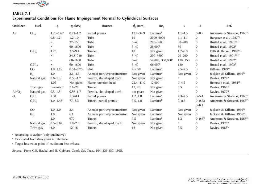
en L R Ref.
rb 1.1–4.5 0–0.7 Anderson & Stresino, 196315
000 3.1–11 0 Hargrave et al., 198775
00 30–200 0 Hustad et al., 199116,17
80 0 Hustad et al., 19926
en 1.7–6.9 0 Fells & Harker, 196880
00 20–200 0 Hustad et al., 199116,17
330,000b 120, 150 0 Hustad et al., 19926
130 0 Hustad et al., 19926
ra 2.5–7.5 0 Kilham, 194913
ra Not given 0 Jackson & Kilham, 195614
en c 0 Davies, 197918
0–4.5 0 Hemeson et al., 198445
en 0.5 0 Davies, 196534
en c 0 Davies, 197918
rb 4.3–7.5 0–5.4 Anderson & Stresino, 196315
rb 0, 8.6 0–0.53 Anderson & Stresino, 196315
0–6.1ra Not given 0 Jackson & Kilham, 195614
ra Not given 0 Jackson & Kilham, 195614
rb 1.3 0–0.67 Anderson & Stresino, 196315
en c 0 Davies, 197918
en 0.5 0 Davies, 196534
TABLE 7.1Experimental Conditions for Flame Impingement Normal to Cylindrical Surfaces
Oxidizer Fuel φ qf (kW) Burner dn (mm) R
Air CH4 1.25–1.67 0.71–1.2 Partial premix 12.7–34.9 Lamina0.8–1.2 1.2–10c Tube 16 2000–8× 37–150 Tube 5–40 200–36× 60–1600 Tube 5–40 26,000b
C3H8 1.25 3.5–9.4 Tunnel 18 Not giv× 34.3–740 Tube 5–40 200–36× 60–1600 Tube 5–40 54,000;
C4H10 × 60–1600 Tube 5–40 66,000b
CO 1.0, 1.19 0.51–0.75 Slot 4 × 50 LaminaH2 1.0 2.1, 4.3 Annular port w/precombustor Not given LaminaNatural gas 0.6–1.3 0.56–1.7 Premix, slot-shaped torch Not given Not giv
1.05 Not given Flame retention head 22.4, 41.0 12,600Town gas Lean-richa 7.1–28 Tunnel 13, 26 Not giv
Air/O2 Natural gas 0.5–1.3 0.56–1.7 Premix, slot-shaped torch not given Not givO2 C2H2 2.34 1.3–4.1 Partial premix 1.2, 1.8 Lamina
C3H8 1.0, 1.43 77, 3.3 Tunnel, partial premix 9.5, 1.8 Lamina
CO 1.0, 2.0 2.4 Annular port w/precombustor Not given LaminaH2 1.0 6.1 Annular port w/precombustor Not given Lamina
1.0 670 Tunnel 9.5 LaminaNatural gas 0.5–1.16 1.7–2.8 Premix, slot-shaped torch Not given Not givTown gas 1.0 12–16 Tunnel 13 Not giv
a According to author (only qualitative).b Calculated from data given in reference.c Target located at point of maximum heat release.
Source: From C.E. Baukal and B. Gebhart, Comb. Sci. Tech., 104, 339-357, 1995.
© 2000 by CRC Press LLC

plane surfaces. Only the results for flame impingement normal to a plane surface are included here. The reader is referred to the literature for further information on angled jets.
7.2.1.4 Flame Parallel to a Plane Surface
This configuration, shown in Figure 7.12, has been the least studied (see Table 7.4). However, it is very important for flight applications. It simulates the heat transfer processes on airfoil surfaces. The studies by Giedt and co-workers (1960, 1966)2,22 investigated flow across the top and bottom of a plane surface. Neither of these studies investigated the heat flux at the leading edge of the target. Beér and Chigier (1968)23 studied impingement only on one side of a plane surface, which was the hearth of a furnace. The flame was inclined at 20° above the horizontal (see Figure 7.12b). Mohr et al. (1996) studied a special configuration for flames parallel to a plane surface which they called radial jet reattachment flames as shown in Figure 7.13.24 This type of flame promises to give more uniform heating of the surface, compared to flames impinging normal to a surface. Figure 7.14 shows the effect of the spacing (S) between adjacent nozzles (air inlet pipe inside radius, R0 = 12.7 mm or 0.5 in.) on the maximum heat flux and surface temperatures.
7.2.2 OPERATING CONDITIONS
Operating conditions have been found to strongly influence the heat transfer intensity. The effects include the oxidizer and fuel composition, flame equivalence ratio and firing rate, Reynolds number at the nozzle exit, burner type, nozzle diameter, and location of the target with respect to the burner.
7.2.2.1 Oxidizers
The most important variable, after the physical configuration, is the oxidizer composition. The oxygen mole fraction in the oxidizer, Ω, has a very large influence on heat transfer intensity. Almost all previous studies used either air (Ω = 0.21) or pure oxygen (Ω = 1.0) as the oxidizer. This affects both the flame temperature and the amount of dissociation in the combustion products. As an example, the adiabatic flame temperatures for methane combusted stoichiometrically with air and with pure oxygen are 2220K and 3054K (3537°F and 5038°F), respectively. Figures 2.4 and 2.5 indicate that the products of combustion for a stoichiometric air/CH4 adiabatic flame contain essentially no unreacted fuel or dissociated species, except at very high flame temperatures approaching adiabatic conditions. However, the combustion products of an O2 /CH4 flame contain nearly 23 vol.% unreacted fuel (CO and H2) and over 18 vol.% dissociated species (H, O, and OH). As these products cool down in the boundary layer along the target surface, they exothermically release heat. This heat release rate from TCHR (see section 4.1.2) may be greater in magnitude than that of the forced convection heat transfer mechanism.
A few studies have used oxygen concentration levels between those of air and pure oxygen. Beér and Chigier23 injected a small, unspecified amount of O2 into an air/coke oven gas flame to raise the temperature slightly. Vizioz and Lowes (1971)25 studied oxygen-enriched air for Ω = 0.30. In related studies, Nawaz (1973)26 and Fairweather et al. (1984)27 studied oxygen-enriched air flames for Ω ranging from 0.46 to 0.61. Davies (1979)18 studied flame impingement heat transfer to a water-cooled tube in crossflow for Ω = 0.23 to 0.35. Ivernel and Vernotte (1979)28 studied oxygen-enriched air/natural gas flames, with Ω ranging from 0.25 to 1.0. Kataoka et al. (1984)29
FIGURE 7.10 Flame impinging normal to a hemi-nosed cylinder.
© 2000 by CRC Press LLC

TABLE 7.2
n L R Ref.
0 1.6–3.8 0 Hargrave & Kilham, 198441
turbulenta 4.6–11 0 Fairweather et al., 198427
0 1.9–15 0 Hargrave et al., 198775
0.02–0.3 0 Kilham & Dunham, 196749
(cf. Dunham, 196376)0.02–0.2 0 Cookson & Kilham, 196336
(cf. Cookson, 196335)(1.3 cm) 0 Conolly & Davies, 19723
0–4.5 0 Hemeson et al., 198445
0.3–1.4 0 Nawaz, 197326
0.3–1.4 0 Fairweather et al., 198427
(40–140 cm) 0 Ivernel & Vernotte, 197928
Not given 0 Kilham & Purvis, 197139
(cf. Purvis, 197477)(1.3 cm) 0 Conolly & Davies, 19723
0.3–1.4 0 Nawaz, 197326
0.3–1.4 0 Fairweather et al., 198474
(1.3 cm) 0 Conolly & Davies, 19723
Not given 0 Kilham & Purvis, 197139
(cf. Purvis, 197477)(1.3 cm) 0 Conolly & Davies, 19723
(1.3 cm) 0 Conolly & Davies, 19723
(1.3 cm) 0 Conolly & Davies, 19723
(40–140 cm) 0 Ivernel & Vernotte, 197928
Experimental Conditions for Flame Impingement Normal to Hemi-nosed Cylinders
Oxidizer Fuel φ qf (kW) Burner dn (mm) Re
Air CH4 1.0 1–8b Tube 16 1200–10,000.943, 1.171 Not given Converging nozzle 12 Laminar & 0.8–1.2 1.2–10b Tube 16 2000–12,00
CO 0.7–1.3 Not given Porous bronze 51 Laminarb
H2 0.5–0.63 Not given Porous bronze 51 Laminarb
Natural gas #2 1.0 Not given Bundle of tubes Not given 50–500Natural gas 1.05 Not given Flame retention head 22.4, 41.0 12,600
Air/O2 CH4 0.62–1.14 3.2 Bundle of tubes 10 Laminarb
0.84–1.14 Not given Bundle of tubes 10 Laminara
Natural gas 0.95 210, 270b Multi-annular w/swirl Not given Not givenO2 CH4 0.95–1.31 Not given Glass torch 10 Laminara
1.0 Not given Bundle of tubes Not given 50–5000.83–1.70 3.8 Bundle of tubes 10 Laminarb
0.83–1.70 Not given Bundle of tubes 10 Laminara
C2H4 1.0 Not given Bundle of tubes Not given 50–500C3H8 1.45–1.83 Not given Glass torch 10 Laminara
1.0 Not given Bundle of tubes Not given 50–500CO 1.0 Not given Bundle of tubes Not given 50–500H2 1.0 Not given Bundle of tubes Not given 50–500Natural gas 0.95 210b Multi-annular w/swirl Not given Not given
a According to author (only qualitative).b Calculated from data given in reference.
Source: From C.E. Baukal and B. Gebhart, Comb. Sci. Tech., 104, 339-357, 1995.
© 2000 by CRC Press LLC

blended O2 and N2 to an equivalent Ω of 0.39.The study by Matsuo et al. (1978)30 was the only study that used a preheated oxidizer. The combustion air was heated to about 500K (440°F) before reaching the burner. Baukal and Gebhart (1998) studied natural gas flames combusted with air, oxygen-enriched air, and pure oxygen.31 They found that the heat transfer to the target was highly dependent on the oxidizer composition (see Chapter 8).
7.2.2.2 Fuels
Another parameter of interest is the fuel composition. Only experiments using gaseous fuels are considered here. Tables 7.1 to 7.4 indicate that natural gas and methane (the main constituent in natural gas) have been the most widely used. Where specified, the specific natural gas compositions are noted in Table 7.5. An example of another fuel used is acetylene, by Schulte (1972).32 The study by Fay33 was the only one in which MAPP® gas was used. This is a stabilized mixture of methylacetylene and propadiene (equivalent to C3.1H5.4), which is produced by Dow Chemical Co. Beér and Chigier23 used another uncommon fuel, coke oven gas, which is a by-product of converting coal to coke. Davies (1965)34 and Shorin and Pechurkin20 used town gas, which is also obtained from coal. Both coke oven gas and town gas are roughly half H2 and a third CH4, with a mixture of other gaseous hydrocarbons. Both fuels have similar heating values and adiabatic flame temper-atures. In one set of tests, Shorin and Pechurkin20 used a mixture of propane and butane in unspecified proportions.
The combination of fuel type and the equivalence ratio φ determines the tendency to produce soot and, therefore, luminous gas radiant emission. This tendency is higher in fuel-rich mixtures (φ > 1). It also increases with higher carbon-to-hydrogen weight ratios in the fuel. For example, C4H10, which has a C:H weight ratio of 4.8, has a higher propensity to produce soot than CH4, which has a C:H weight ratio of 3.
7.2.2.3 Equivalence Ratios
This ratio directly affects both the sooting tendency and the level of dissociation in the combustion products. Fuel-rich flames (φ > 1) produce a combination of both luminous and nonluminous thermal radiation. The combustion products of these flames may also contain unreacted fuel components, due to insufficient oxygen. Fuel-lean flames (φ < 1) normally do not produce luminous thermal radiation, due to the absence of soot particles. These flames seldom produce significant quantities of unreacted fuel species unless the flame temperature is high enough to produce dissociation. Flames at or near stoichiometric (φ = 1) produce the highest flame temperatures, due
FIGURE 7.11 Flame impinging normal to a plane surface. (From C.E. Baukal and B. Gebhart, Int. J. Heat Fluid Flow, 17(4), 386-396, 1996.)
© 2000 by CRC Press LLC

L R Ref.
5–9 0–7 Matsuo et al., 197830
2.4 0–1.3 Anderson & Stresino, 196315
13–65 0–4 Buhr et al., 197366
(cf. Buhr, 196985)10, 16 0–60 Milson & Chigier, 19739
13–64 0–10 Kremer et al., 197421
(cf. Buhr, 196985)7.5 0–3 Posillico, 198648
2, 3, 4 0–5 Eibeck et al., 19938
1.3–13 0–2.5 Schulte, 197232
23, 32 0–17 Veldman et al., 197542
5.7–11 0–4.6 Vizioz & Lowes, 197125
0–8.4 0–3.5 Smith & Lowes, 197437
2–20 0–5 Hoogendoorn et al., 197852
(60–100 cm) (0–37 cm) Rajani et al., 197838
2–20 0–10 Popiel et al., 198053
7.3 0–7.3 You, 19857
16–27 0 Horsley et al., 198246
(cf. Tariq, 198247)1–12 0 van der Meer, 199154
0.93 0–8.11 Mohr et al., 199524
0–1700–100
0–1000–60
Rigby and Webb, 199544
0.5–6.0 0–1.0 Baukal and Gebhart, 199831
TABLE 7.3 Experimental Conditions for Flame Impingement Normal to Plane Surfaces
Oxidizer Fuel φ qf (kW) Burner dn (mm) Ren
Air Coke oven gas Not given 606 Tunnel w/air preheat 100 Turbulentc
CH4 1.33, 1.67 0.71 Partial premix 13, 16 Laminarc
2.58–2.76 1.0–160 Partial premix 7.8 17,680–22,700
4.8, × 46–220c Tube 12.7 7000–35,3002.75 1.0–160 Partial premix 7.8 17,680–22,700
0.51 0.7c Long tube w/precombustor
9.5 3100
0.78 22 Premixpremix, pulsed
50 66309700
C2H2 1.0 Not given Premix torch 2.0 Laminara
C3H8 1.0 1.2, 1.5 Premix tube w/stainless steel mesh
25 1300c
Natural gas #1 0.95 2100 Variable swirl 131.3–152.0 Turbulentc
Natural gas 1.0 1000–1500 Tunnel 172 Turbulentc
Natural gas #3 1.0 Not given Tunnel 13.8 1050, 1860Natural gas #2 1.0 1000, 1500 Tunnel Not given Not givenNatural gas #3 1.0 Not given Tunnel 13.8 1050, 1860Natural gas #5 × 1.67, 8.51 Tube 55 70, 356
Air Natural gas 1.05 0.3, 0.4c Flame retention head 5.6–15.3 7050–16,200
Natural gas #4 1.0 Not given Tunnel 13.8, 27.6 1700–4250Natural gas 0.65–2.79 39.7 Co-axial radial jet
reattachment flame63.5 3640–24,600
Natural gas × 10.55.1, 10.5
Tube 3.816.35
50001450, 3000
Natural gas #6 1.0 5 Flame working torch 38.5 2910
© 2000 by CRC Press LLC

–14 0–5 Shorin & Pechurkin, 196820
–20 0–3 Kataoka et al., 198429
.7 0–4.8 Vizioz & Lowes, 197125
.5–6.0 0–1.0 Baukal and Gebhart, 199831
.74, 2.1 0 Kilham & Purvis, 197857
(cf. Purvis, 197477).3 0–36 Anderson & Stresino, 196315
(0–1.3 cm) Fay, 196733
.60–130–29
Anderson & Stresino, 196315
(0–1.3 cm) Fay, 196733
.74, 2.1 0 Kilham & Purvis, 197857
(cf. Purvis, 197477), 8 0 Rauenzahn, 19865
–8 0 Shorin & Pechurkin, 196820
.3 0–12 Anderson & Stresino, 196315
0–2.50–10
Reed, 196343
(0–1.3 cm) Fay, 196733
.2–29 0–9.5 Schulte, 197232
0–100 cm) (0–37 cm) Rajani et al., 197838
.5–6.0 0–1.0 Baukal and Gebhart, 199831
TABLE 7.3 (continued)
L R Ref.
Town gas + 0.67–0.95 Not given Water-cooled tube w/precombustor
25, 46 1500–19,000 0
Air/O2 CH4 0.61 Not given Converging nozzle w/precombustor
10 857–2000 2
Natural gas #1 0.95 2100, 3000 Variable swirl 115.4 Turbulentc 8Natural gas #6 1.0 5–25 Flame working torch 38.5 1850–9200 0
O2 CH4 0.95–1.31 Not given Premixed multiport 9.5 489–549 0
C2H2 2.34 4.1 Partial premix 1.8 Laminarc 40.9–2.5 2.9 Premix welding torch Not given Turbulentc b
O2 C3H8 1.01.43
2.778
Tunnel, partial premix 1.89.5
Laminarc 18
1.0–2.0 2.9 Premix torch Not given Turbulentc b1.45–1.83 Not given Premixed multiport 9.5 551–692 0
1.0 61, 94 Premix welding torch 25 Turbulentc 6C3H8 + C4H10 0.83–1.0 34 Water-cooled tube
w/precombustor25 300–1200 0
H2 1.0 105 Tunnel 9.5 Laminarc 10.851.1
5.42.8
(2) Glass working torches
275.6
2000c
4600c
29
MAPP gas 0.85–2.2 2.9 Premix welding torch Not given Turbulentc bNatural gas 1.0 Not given Premix torch 0.53, 1.7 Laminara 1Natural gas #2 1.0 1000–1750 (2) Commercial
burnersNot given Not given (6
Natural gas #6 1.0 5–25 Flame working torch 38.5 810–4050 0
a According to author (only qualitative).b Tip of inner flame cone just touching target.c Calculated from data given in reference.Source: From C.E. Baukal and B. Gebhart, Comb. Sci. Tech., 104, 339-357, 1995.
Experimental Conditions for Flame Impingement Normal to Plane Surfaces
Oxidizer Fuel φ qf (kW) Burner dn (mm) Ren
© 2000 by CRC Press LLC

to complete combustion. They also generally produce only nonluminous radiation since no soot is generated.
Most of the studies used stoichiometric mixtures. Cookson and Kilham (1963)35,36 and Davies34
used equivalence ratios as fuel lean as φ = 0.5. Milson and Chigier,9 You,7 and Hustad and co-workers6,16,17 used pure fuel jets (φ = ×). Many studies have investigated a range of equivalence ratios in order to determine the resulting effects on heat transfer to the target. Davies34 used lean and rich mixtures. The actual equivalence ratios were not specified.
7.2.2.4 Firing Rates
The firing rate or gross heat release (qf) of the flames has ranged from 0.3 to 3000 kW (103 to 107
Btu/hr). Large industrial-scale flames were used by Beér and Chigier,23 Vizioz and Lowes,25 Smith and Lowes (1974),37 and Rajani et al. (1978)38 at the International Flame Research Foundation (IFRF) in IJmuiden, The Netherlands. Beér’s flame impinged downward on the hearth of a furnace. In the other three studies, the flames impinged on water-cooled targets located inside a furnace environment. Many of the studies (e.g., see Reference 39) considered here used torch tips, firing at under 50 kW (170,000 Btu/hr).
7.2.2.5 Reynolds Number
The Reynolds number at the burner nozzle, Ren, varied from 50 to 330,000. Both laminar (e.g., see Reference 27) and turbulent (e.g., see Reference 40) flow conditions arose. As shown in Tables 7.1 to 7.4, the Reynolds number was not always given. For some studies, the flows were indicated to be either laminar or turbulent. In other studies, the nozzle Reynolds number was estimated from other information, such as nozzle diameter and gas flow rates.
The Reynolds number varies directly with the burner diameter. It is also influenced by burner design. In partially or fully premixed flames, the combustion products leave the burner at an elevated temperature. However, in diffusion flames, the gases leave the burner at essentially ambient con-ditions. Since the gas viscosity increases with temperature, Ren is generally lower if the gases have been heated at the burner exit. In some studies, turbulence effects were analyzed (e.g., see Reference 41). However, in most studies, the turbulence effects were not assessed.
7.2.2.6 Burners
Many different types of burners have been used. These range from fully premixed to diffusion mixing, downstream of the burner exit. In fully premixed burners, the fuel and oxidizer mix prior to reaching the nozzle exit (see Figure 1.10). An example was the study by Veldman et al. (1975), where premixed gases were fired in a burner consisting of a tube with a stainless steel mesh.42 The
(a)
(b)
FIGURE 7.12 Flames impinging (a) parallel and (b) oblique to a plane surface.
© 2000 by CRC Press LLC

R Ref.
0–10 Beér & Chigier, 196823
(1.3–14 cm) Giedt et al., 19602
(1.3–14 cm) Woodruff & Giedt, 196622
ith permission.)
TABLE 7.4Experimental Conditions for Flame Impingement Parallel to Plane Surfaces
Oxidizer Fuel φ qf (kW) Burner dn (mm) Ren L
Air Coke oven gas 1.0 1470 Concentric tubes 150 4800–270,000 9O2 C2H2 2.5 Not given (30) Multihead torch tips Not given Turbulenta Not given
2.5 Not given Multihead torch tips Not given Laminara Not given
a According to author (only qualitative).
Source: From C.E. Baukal and B. Gebhart, Comb. Sci. Tech., 104, 339-357, 1995.
FIGURE 7.13 Pair of radial jet reattachment flames. (Courtesy of ASME, New York.24 W
© 2000 by CRC Press LLC
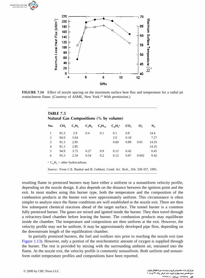
resulting flame in premixed burners may have either a uniform or a nonuniform velocity profile, depending on the nozzle design. It also depends on the distance between the ignition point and the exit. In most studies using this burner type, both the temperature and the composition of the combustion products at the burner exit were approximately uniform. This circumstance is often simpler to analyze since the flame conditions are well established at the nozzle exit. There are then few subsequent chemical reactions ahead of the target surface. The tunnel burner is a common fully premixed burner. The gases are mixed and ignited inside the burner. They then travel through a refractory-lined chamber before leaving the burner. The combustion products may equilibrate inside the chamber. The temperature and composition are then uniform at the exit. However, the velocity profile may not be uniform. It may be approximately developed pipe flow, depending on the downstream length of the equilibration chamber.
In partially premixed burners, the fuel and oxidizer mix prior to reaching the nozzle exit (see Figure 1.13). However, only a portion of the stoichiometric amount of oxygen is supplied through the burner. The rest is provided by mixing with the surrounding ambient air, entrained into the flame. At the nozzle exit, the velocity profile is commonly nonuniform. Both uniform and nonuni-form outlet temperature profiles and compositions have been reported.
FIGURE 7.14 Effect of nozzle spacing on the maximum surface heat flux and temperature for a radial jet reattachment flame. (Courtesy of ASME, New York.24 With permission.)
TABLE 7.5Natural Gas Compositions (% by volume)
No. CH4 C2H6 C3H8 C4H10 CmHna CO2 O2 N2
1 81.3 2.9 0.4 0.1 0.1 0.8 14.42 84.9 5.64 2.0 0.18 7.273 81.3 2.85 0.60 0.89 0.01 14.354 81.3 2.85 14.355 94.9 3.75 0.27 0.9 0.12 0.42 0.416 95.3 2.54 0.54 0.2 0.12 0.87 0.002 0.42
a CmHn = other hydrocarbons.
Source: From C.E. Baukal and B. Gebhart, Comb. Sci. Tech., 104, 339-357, 1995.
© 2000 by CRC Press LLC
In diffusion-mixing burners, the fuel and oxidizer begin to mix at the nozzle exit (see Figure 1.12), where the velocity is often nonuniform. An example is the glass working torches used
by Reed (1963).43 In diffusion burners, the exit temperature field is commonly homogeneous and equal to ambient conditions. The gas composition at the exit is pure fuel and pure oxidizer, with no combustion products. If the oxidizer is not supplied through the burner, a pure diffusion flame results. The oxygen is provided for combustion by ambient air entrainment into the flame.
7.2.2.7 Nozzle Diameter
In the configurations considered here, the exiting flame shape was round, except for those used by Kilham13 and Davies,18 which were slot shaped. The burner nozzle diameter, dn, ranged from 0.53 to 152 mm (0.02 to 6.0 in.). This dimension was not given in some of the studies listed in Tables 7.1 to 7.4. In many studies (e.g., see Reference 3), the burner outlet consisted of a nested bundle of small tubes or orifices, arranged in a circular pattern. This is common practice for nozzles used on cutting and welding torches.
7.2.2.8 Location
The dimensionless axial distance between the burner exit and the target, L, varied from 0 to 200. In most studies, it was less than about 20. This distance has a strong influence on the resulting heat transfer to the target. Shorter distances result in higher flux rates. One cause is less ambient air entrainment. Another reason is that the flame widens at longer distances. This diffuses the heat flux over a wider cross-sectional area. Fay33 adjusted the axial position of a premixed torch flame so that the inner flame cone tip touched the target. The specific axial locations were not given. Davies18 positioned water-cooled tubes at the location in the flame that produced the highest heating rate. This location varied with the oxidizer composition and the equivalence ratio. Again, no dimensions were reported. For flames parallel to plane surfaces, L is taken as the distance from the burner to the leading edge of the target.
The dimensionless radial distance, R, from the nozzle centerline to the location on the target where the heat flux was measured is an important parameter. The heat flux at the stagnation point (R = 0) was measured in every study. In most of the experiments of jet flames impinging normal to plane surfaces, the radial heat flux profile was measured. The radial distance, R, ranged from 0 to as high as 60. In general, the heat flux decreased with R. However, in several studies, the peak heat flux did not occur at the stagnation point of the target. For example, Milson and Chigier9
measured a peak flux at R ranging from 6 to 29, depending on the nozzle exit Reynolds number. The turbulent mixing of ambient air with the pure jets of CH4 (φ = ×) was given as the cause. In the study by Rigby and Webb (1995), the heat flux to a wide range of both axial (L = 0 to 170) and radial (R = 1 to 100) locations was investigated.44
Table 7.6 indicates the studies in which the target was located inside a furnace. This influences the heat transfer in two important ways. The radiation from the hot refractory walls to the target is a significant portion of the total heat flux to the target. Vizioz and Lowes25 and Smith and Lowes37
showed that this effect was comparable in magnitude to the forced convection effect at the target. Ivernel and Vernotte28 calculated this effect to be up to 42% of the total heat flux to a hemi-nosed cylinder. Also, any gases entrained into the jet are hot combustion products, instead of ambient air, as in most studies. Therefore, the flame jet is not cooled as much as in tests done at ambient conditions.
7.2.3 STAGNATION TARGETS
Tables 7.7 to 7.10 tabulate the important features of the targets. These include the dimensions, compositions, surface conditions, and temperature level for each of the four configurations. These
© 2000 by CRC Press LLC

TABLE 7.6
properties varied widely among the studies reviewed here. In some studies, these were varied to examine the effect on the heat transfer mechanisms. These are discussed further below.
7.2.3.1 Size
The targets ranged in size from a 0.56 cm (0.22 in.) o.d. disk to a 200 × 625 cm (6.6 × 20.5 ft) furnace hearth. Most of the cylindrical targets have been hollow pipes. Kilham13 and Jackson and Kilham14 used solid refractory rods. Hustad et al.6,16,17 used solid steel cylinders. All of the heminosed cylinders were under 22 mm (0.87 in.) o.d., except for those used by Hemeson et al. (1984),45 which were from 50 to 150 mm (2 to 6 in.). Most of the plane surfaces in Table 7.9 were disks of over 16 mm (0.63 in.) in diameter, except for the 0.56 mm (0.022 in.) o.d. disks used by Horsley et al. (1982).46,47 In addition to disks, many studies used square and rectangular plates as the target surfaces.
Flame Jet Impingement Studies with the Target in a Furnace
Ref.Furnace Wall Temp.
(K)Furnace Dimensions
(m)
Beér and Chigier, 196823 1200–1500 2 W × 2 H × 6.25 LVizioz and Lowes, 197125 Not given 2 W × 2 H × 6.25 LSmith and Lowes, 197437 Not given 2 W × 2 H × 6.25 LMatsuo et al., 197830 1300–1500 2.16 W × 1.80 H × 1.36 LRajani et al., 197838 770–1870 1.0 dia. × 4.5 LIvernel and Vernotte, 197928 1650–2000 0.6 dia. × 2.05 L
Source: From C.E. Baukal and B. Gebhart, Comb. Sci. Tech., 104, 339-357, 1995.
TABLE 7.7Stagnation Targets for Flames Impinging Normal to Cylindrical Surfaces
Ref.db
(mm) MaterialSurface Coating(s)
or Treatmenttw
(K)
Kilham, 194913 3 Sillimanite Al2O3, FeO, Cr2O3, uranium oxide
1220–1630
Jackson & Kilham, 195614 3.2 Sillimanite Al2O3, FeO, Cr2O3, uranium oxide
950–1445
Anderson & Stresino, 196315 0.91, 1.5 Copper None <373Davies, 196534 1.5 Stainless steel None <373
3.2 Copper None <373Fells & Harker, 196880 50 Stainless steel None <373Davies, 197918 2.7 Stainless steel None 300Hemeson et al., 198445 32.6–59.8 Not given None Not givenHargrave et al., 198775 22 Brass None 378Hustad et al., 199116,17 50 Steel None 520–620Hustad et al., 19926 50 Steel None 520–570
Source: From C.E. Baukal and B. Gebhart, Comb. Sci. Tech., 104, 339-357, 1995.
© 2000 by CRC Press LLC

TABLE 7.8
7.2.3.2 Target Materials
The most commonly used materials were aluminum, copper, brass, and stainless steel. For example, Posillico (1986) studied flames impinging normal to uncoated aluminum disks.48 Aluminum, copper, and brass have very high internal thermal conductivities. Therefore, they are easier to water-cool since the heat from the impinging flame is conducted away quickly. However, these materials also have relatively low melting points. For that reason, they have not been used at very high surface temperatures. Refractories, including alumina (Al2O3) and sillimanite (Al2SiO5), were also used.
7.2.3.3 Surface Preparation
Most of the target surfaces were untreated. However, in some experiments, the surfaces were treated or coated to study a specific surface effect. Kilham13 and Jackson and Kilham14 coated the surface of their refractory cylinders with different oxides. The objective was to estimate the emissivities of the coatings. The surface temperature was approximately determined using a thermocouple imbedded inside the cylinder body. Radiation from the surface was measured with a thermopile. Using the temperature level and the radiation, along with an energy balance on the cylinder, the emissivity of the coatings was calculated as a function of temperature.
Four studies used coatings to determine the effects of surface catalysis on the heat transfer from an impinging flame. Giedt et al.2 used both uncoated and porcelain-coated iron plates. These surfaces were considered to be catalytic and noncatalytic, respectively. The measured heat flux for these two surface conditions was about the same. It was concluded that surface chemical recombination effects were negligible for those test parameters. Kilham and Dunham (1967)49 used three different surface conditions to study the effects on air/CO flames impinging on a hemi-nosed cylinder. The results indicated that the lowest heat flux was for the National Bureau of Standards Coating A418, which is a mixture of eight oxides. It was assumed to be noncatalytic. On the other hand, the highest flux was found for a platinum coating, which was considered to be perfectly catalytic. The heat flux to an uncoated copper heat flux gage surface was intermediate between the results for the A418 and platinum coatings. However, the differences were small. It was concluded that the bulk of the chemical reactions occurred in the boundary layer. In addition, as L increased, the heat flux for all three surface conditions converged to the same value. Conolly and Davies3,50 found no difference in
Stagnation Targets for Flames Impinging Parallel to Hemi-nosed Cylinders
Ref.db
(mm) MaterialSurface Coating(s)
or Treatmenttw
(K)
Cookson & Kilham, 196335 14 Brass None >373Kilham & Dunham, 196749 22.2 Brass None, A418, Pt >373Kilham & Purvis, 197139 9.5 Stainless steel None 290–470Conolly & Davies, 19723
(cf. Conolly, 197150)12.7 Stainless steel None, SiO2, Pt 400
Nawaz, 197326 9.5 Brass None 290–420Ivernel & Vernotte, 197928 46 Inconel None 600–1400Fairweather et al., 198427 9.5 Brass None 340–1600Fairweather et al., 198440 9.5 Brass None ~378Hargrave & Kilham, 198441 22 Brass None 393Hemeson et al., 198445 50–150 Not given None Not givenHargrave et al., 198775 22 Brass None 418
Source: From C.E. Baukal and B. Gebhart, Comb. Sci. Tech., 104, 339-357, 1995.
© 2000 by CRC Press LLC
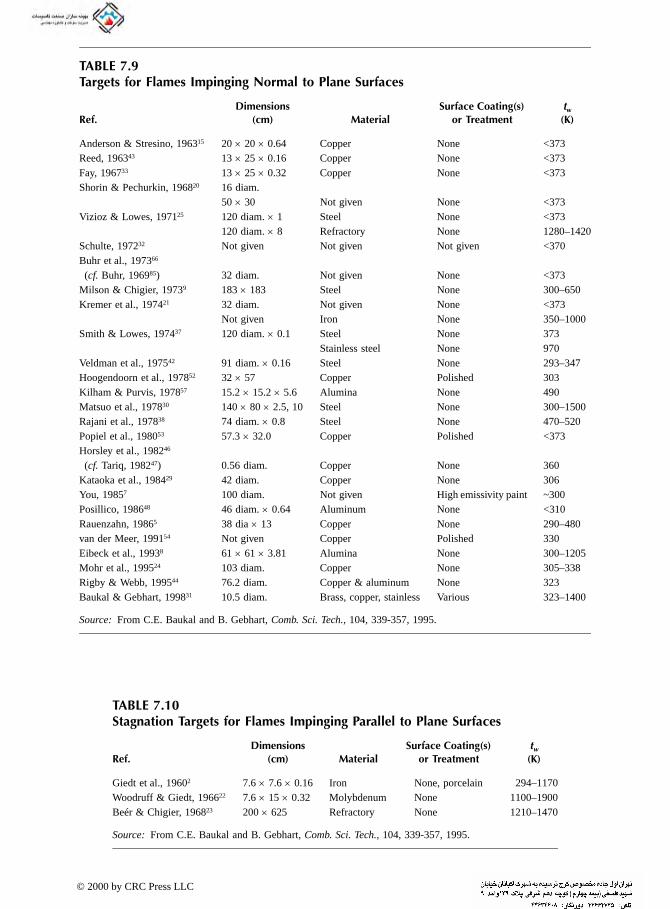
TABLE 7.9
Targets for Flames Impinging Normal to Plane Surfaces
Ref.Dimensions
(cm) MaterialSurface Coating(s)
or Treatmenttw
(K)
Anderson & Stresino, 196315 20 × 20 × 0.64 Copper None <373Reed, 196343 13 × 25 × 0.16 Copper None <373Fay, 196733 13 × 25 × 0.32 Copper None <373Shorin & Pechurkin, 196820 16 diam.
50 × 30 Not given None <373Vizioz & Lowes, 197125 120 diam. × 1 Steel None <373
120 diam. × 8 Refractory None 1280–1420Schulte, 197232 Not given Not given Not given <370Buhr et al., 197366
(cf. Buhr, 196985) 32 diam. Not given None <373Milson & Chigier, 19739 183 × 183 Steel None 300–650Kremer et al., 197421 32 diam. Not given None <373
Not given Iron None 350–1000Smith & Lowes, 197437 120 diam. × 0.1 Steel None 373
Stainless steel None 970Veldman et al., 197542 91 diam. × 0.16 Steel None 293–347Hoogendoorn et al., 197852 32 × 57 Copper Polished 303Kilham & Purvis, 197857 15.2 × 15.2 × 5.6 Alumina None 490Matsuo et al., 197830 140 × 80 × 2.5, 10 Steel None 300–1500Rajani et al., 197838 74 diam. × 0.8 Steel None 470–520Popiel et al., 198053 57.3 × 32.0 Copper Polished <373Horsley et al., 198246
(cf. Tariq, 198247) 0.56 diam. Copper None 360Kataoka et al., 198429 42 diam. Copper None 306You, 19857 100 diam. Not given High emissivity paint ~300Posillico, 198648 46 diam. × 0.64 Aluminum None <310Rauenzahn, 19865 38 dia × 13 Copper None 290–480van der Meer, 199154 Not given Copper Polished 330Eibeck et al., 19938 61 × 61 × 3.81 Alumina None 300–1205Mohr et al., 199524 103 diam. Copper None 305–338Rigby & Webb, 199544 76.2 diam. Copper & aluminum None 323Baukal & Gebhart, 199831 10.5 diam. Brass, copper, stainless Various 323–1400
Source: From C.E. Baukal and B. Gebhart, Comb. Sci. Tech., 104, 339-357, 1995.
TABLE 7.10Stagnation Targets for Flames Impinging Parallel to Plane Surfaces
Ref.Dimensions
(cm) MaterialSurface Coating(s)
or Treatmenttw
(K)
Giedt et al., 19602 7.6 × 7.6 × 0.16 Iron None, porcelain 294–1170Woodruff & Giedt, 196622 7.6 × 15 × 0.32 Molybdenum None 1100–1900Beér & Chigier, 196823 200 × 625 Refractory None 1210–1470
Source: From C.E. Baukal and B. Gebhart, Comb. Sci. Tech., 104, 339-357, 1995.
© 2000 by CRC Press LLC

heat flux between a surface coated with highly catalytic platinum and a surface coated with SiO2, which was expected to be noncatalytic. This again led to the conclusion that the recombination of
radical species occurs in the boundary layer prior to reaching the surface. Baukal and Gebhart (1997) also found no difference in heat flux to surfaces coated with alumina or platinum.51
You7 used a high-emissivity (0.96) paint to maximize the amount of radiant heat absorbed by the target. Three interrelated studies52-54 used polished copper surfaces to reduce the effects of flame radiation. In some studies, the heat flux gage surface was coated or treated, as discussed in Chapter 6.
7.2.3.4 Surface Temperatures
Surface temperatures ranged from 290K to 1900K (63°F to 2960°F). For many measurements, the temperature, tw, was maintained below 373K (212°F), using water-cooled targets. In some studies (e.g., Hargrave and Kilham, 198441,45), the surface temperature was slightly above 373K (212°F). This eliminated the possibility of combustion products condensing on the target. Ethylene glycol was used as the target coolant because it has a higher boiling temperature than water. Beér and Chigier23 and Vizioz and Lowes25 measured surface temperatures above 1200K (1700°F) for refrac-tory targets. In some studies, the surface temperature level was actually for the heat flux gage, and not the target. For example, Fairweather et al.27 reported a maximum surface temperature of 1600K (2400°F). However, the target was made of brass, which melts at about 1300K (1900°F). A stainless steel heat flux gage imbedded in the brass target was used to measure the heat flux. Stainless steels have a melting point of about 1700K (2600°F).
7.2.4 MEASUREMENTS
Experimental measurement techniques used in flame impingement studies were discussed in Chapter 6. Table 7.11 shows the measured heat fluxes, gas temperatures, and gas velocities for the air/fuel flame impingement studies for all geometries. Table 7.12 is similar except for air/O2 /fuel studies, and Table 7.13 is for O2 /fuel studies. Table 7.14 is a compilation of the maximum reported ranges for the total heat flux at the given gas temperatures using the five methods of measuring heat flux that were used in the flame impingement studies. Table 7.15 gives the maximum temper-ature ranges for all studies for the various methods used to measure gas temperature. Table 7.16 lists all of the flame impingement studies that used the line reversal method to measure gas temperature. Table 7.17 gives the details of all experiments that used fine wire thermocouples to measure gas temperatures. Table 7.18 gives details of the experiments that used Pitot probes to measure gas velocity. Table 7.19 shows the studies that measured gas composition, which gases were measured, and what techniques were used to measure them.
7.3 SEMIANALYTICAL HEAT TRANSFER SOLUTIONS
This chapter section is taken from a review paper by Baukal and Gebhart (1996).10 Heat transfer from high-temperature gases to axisymmetric and blunt-nosed bodies has been studied for many years. These processes are very important in aerospace applications. Aerospace vehicles, such as rockets and missiles, travel at high supersonic velocities. Commonly, the nose of these surfaces is axisymmetric, blunt, and rounded. Gas shock-waves are produced as the vehicles travel through the atmosphere. The resulting temperatures at the stagnation point are generally high enough to cause the atmospheric gases to dissociate into many chemical species. Very high heat fluxes arise in that region. Several semianalytical solutions have been proposed for calculating such fluxes. Those solutions were derived from the laminar, two-dimensional, axisymmetric boundary layer equations applied in the stagnation region. The equations were simplified using similarity flow formulations. In the resulting heat flux solutions, a constant was numerically determined. Therefore, the solutions are referred to as semianalytical.
© 2000 by CRC Press LLC

TABLE 7.11 y for Air/Fuel Studies
tj Gas Velocity, vj
(K) Method (m/sec)
1213–1633 Calculated 5–30a
s 1179–1659 Calculated 8–20a
Not given Calculated 0.3–381360–1450 Not measured —2260 Not measured —1624–1910 Not measured —1370–1950 Pitot tube Not given2500–2750 Not measured —Not given Uncooled Pitot-static probe Not given1450–1850 5-hole Pitot-static probe 2.8–46
2200 Cooled Pitot tube Not given— Not measured —573-1923 Not measured —430–2200 Not measured —
Not given Not measured —
1170–2020 1- & 5-hole Pitot-static probe 6–195292–419 Not measured —370–2100 Cooled Pitot tube & LDV 2–541200–1600 Pitot tube 20–82460–1950 1- & 5-hole Pitot-static probe 0.91–872225 Not measured —370–2100 Cooled Pitot tube & LDV 2–54
1643–2165 Not measured —
Experimental Methods and Ranges for Total Heat Flux, Gas Temperature, and Velocit
Total Heat Flux, q″ Gas Temperature,
Year Author(s) Method (kW/m2) Method
1949 Kilham13 Steady-state uncooled target 70–130a Line reversal1956 Jackson & Kilham14 Steady-state uncooled target 20–107a (6) Decreasing diam. uncoated T/C1963 Anderson & Stresino15 Steady-state cooled target 32–1100 Adiabatic equilibrium calculation
Cookson & Kilham35 Steady-state cooled gage 73–180 (7) Decreasing diam. coated T/Cs1965 Davies34 Steady-state cooled target 570–950 Line reversal1967 Kilham & Dunham49 Steady-state cooled gage 41–95 (7) Decreasing diam. coated T/Cs1968 Beér & Chigier23 Steady-state cooled gage 15–54 Suction pyrometer
Fells & Harker80 Steady-state cooled target 250–840 Line reversalShorin & Pechurkin20 Steady-state cooled gage Nondimen. Uncoated T/C
1971 Vizioz & Lowes25 Steady-state cooled target 24–280 Suction pyrometer1972 Conolly & Davies3
(cf. Conolly, 197150) Transient uncooled gage Nondimen. Line reversalSchulte32 Steady-state cooled gage 79–620 Not measured
1973 Buhr et al.66 Steady-state cooled gage 110–440 Uncoated T/CMilson & Chigier9 Transient uncooled target 1.3–13 Coated T/C
1974 Kremer et al.21 Steady-state cooled gageTransient uncooled gage 120–450
120–470 Coated T/CSmith & Lowes37 Steady-state cooled target
Steady-state cooled gage 180–45057–150 Suction pyrometer
1975 Veldman et al.42 Transient uncooled target 0.086–1.8 Coated T/C1978 Hoogendoorn et al.52 Steady-state cooled gage 0–560 Coated T/C
Matsuo et al.30 Transient uncooled target 23–350 Uncoated T/CRajani et al.38 Steady-state cooled target 262–421 Suction pyrometer
1979 Davies18 Steady-state cooled target 330–650 Adiabatic equilibrium calculation1980 Popiel et al.53 Steady-state cooled gage 100–630 Coated decreasing diam. T/Cs1982 Horsley et al.46
(cf. Tariq, 198247) Transient uncooled gage 220–440 Uncoated T/C
© 2000 by CRC Press LLC
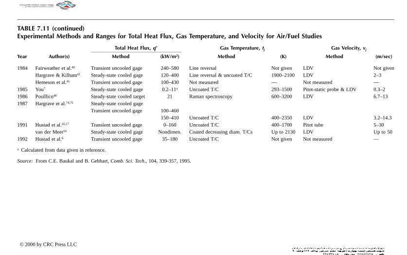
0 Line reversal Not given LDV Not given0 Line reversal & uncoated T/C 1900–2100 LDV 2–30 Not measured — Not measured —a Uncoated T/C 293–1500 Pitot-static probe & LDV 0.3–2
Raman spectroscopy 600–3200 LDV 6.7–13
00 Uncoated T/C 400–2350 LDV 3.2–14.3
Uncoated T/C 400–1700 Pitot tube 5–30en. Coated decreasing diam. T/Cs Up to 2130 LDV Up to 500 Uncoated T/C Not given Not measured —
, 1995.
Gas Temperature, and Velocity for Air/Fuel Studies
Gas Temperature, tj Gas Velocity, vj
2) Method (K) Method (m/sec)
1984 Fairweather et al.40 Transient uncooled gage 240–58Hargrave & Kilham41 Steady-state cooled gage 120–40Hemeson et al.45 Transient uncooled gage 100–43
1985 You7 Steady-state cooled gage 0.2–111986 Posillico48 Steady-state cooled target 211987 Hargrave et al.74,75 Steady-state cooled gage
Transient uncooled gage 100–46150–41
1991 Hustad et al.16,17 Transient uncooled gage 0–160van der Meer54 Steady-state cooled gage Nondim
1992 Hustad et al.6 Transient uncooled gage 35–18
a Calculated from data given in reference.
Source: From C.E. Baukal and B. Gebhart, Comb. Sci. Tech., 104, 339-357
TABLE 7.11 (continued) Experimental Methods and Ranges for Total Heat Flux,
Total Heat Flux, q″
Year Author(s) Method (kW/m
© 2000 by CRC Press LLC

TABLE 7.12
The heat transfer from impinging, chemically active flames has also been extensively studied. The experimental conditions and measurements for those studies have been previously reviewed56
and discussed above. In 12 of those studies,3,26-28,35,39,41,45,46,49,54,57 the measured heat flux was compared against one or more semianalytical solutions. The stagnation body has commonly been a hemispherically nosed cylinder (see Figure 7.15). This geometry has been used because of its similarity to the shape of aerospace vehicles. Then, the semianalytical heat transfer solutions, derived for aeronautical applications, were used to model the measured heat fluxes in energetic flame impingement. The applicability of those equations to flame heating applications has been determined. In aerospace applications, the vehicle moves through stagnant atmospheric gases. In impinging flames, the combustion products move around a stationary target. Therefore, the relative motion is similar in both applications.
Chen and McGrath (1969)58 reviewed impingement heat transfer from combustion products containing dissociated species. Sample heat transfer calculations were given for a stoichiometric O2 /C3H8 flame impinging on a 2 cm (0.8 in.) o.d. sphere. The equations recommended by McAdams (1954),59 Altman and Wise (1956),60 and Rosner (1961)61 were used. The Lewis number, Le, is the ratio of the mass diffusion rate to the thermal diffusion effect (see Chapter 2). The results were evaluated for both Le = 1 and Le > 1. It was concluded that, for Le = 1, the existing information was sufficient to adequately predict heat transfer in chemically reacting systems. However, for flows in which Le > 1, more analytical and experimental work was recommended. Such systems are important for high-temperature flames, where considerable dissociation occurs.
Two types of heat transfer behavior have been compared with experimental data from the studies considered here (see Table 7.20). The first was forced convection with no chemical dissociation. This is applicable in lower temperature-level flame impingement. The second was forced convection with dissociation. The heat transfer relations for the second type have been variations of those recommended for the first type. These equations are useful in predicting the heat transfer in the absence of experimental data.
Experimental Methods and Ranges for Total Heat Flux, Gas Temperature, and Velocity for Air/O2 /Fuel Studies
Total Heat Flux, q″ Gas Temperature, tj Gas Velocity, vj
Year Author(s) Method (kW/m2) Method (K) Method (m/sec)
1971 Vizioz & Lowes25
Steady-state cooled target
26.5 Suction pyrometer 1850–1950 Not measured
—
1973 Nawaz26 Transient uncooled gage
1400–2600 Line reversal 2600–2763 Calculated Not given
1979 Davies18 Steady-state cooled target
600–1600 Adiabatic equilibrium calculation
2380–2875 Not measured
—
Ivernel & Vernotte28
Transient uncooled gage
50–1200 Twin sonic orifice probe
1640–2750 Cooled Pitot-static probe
5–51
1984 Fairweather et al.74
Transient uncooled gage
1400–2600 Line reversal 2710–2760 Calculated 32–36
Kataoka et al.29
Steady-state cooled gage
Nondimen. Uncoated T/C 820–1720 Uncooled Pitot tube
7.4 – 45.1
Source: From C.E. Baukal and B. Gebhart, Comb. Sci. Tech., 104, 339-357, 1995.
© 2000 by CRC Press LLC

TABLE 7.13
Experimental Methods and Ranges for Total Heat Flux, Gas Temperature and Velocity for O2 /Fuel Studies
Total Heat Flux, q″ Gas Temperature, tj Gas Velocity, vj
Year Author(s) Method (kW/m2) Method (K) Method (m/sec)
1956 Jackson & Kilham14
Steady-state uncooled target
27–58a (6) Decreasing diam. uncoated T/Cs
1394–1468 Calculated 3–6a
1960 Giedt et al.2 Transient uncooled target
200–670 Not measured — Not measured —
1963 Anderson & Stresino15
Steady-state cooled target
32–41000 Adiabatic equilibrium calculation
Not given Calculated 43–1400
Reed43 Steady-state cooled target
0–1450 Adiabatic equilibrium calculation
3080 Calculated 7.5, 10
1965 Davies34 Steady-state cooled target
3500–5500 Line reversal 2260 Not measured —
1966 Woodruff & Giedt22
Transient uncooled target
Nondimen. Line reversal 2900–3200 Cooled Pitot tube
40–64
1967 Fay33 Steady-state cooled target
0–5600 Not measured — Not measured —
1968 Shorin & Pechurkin20
Steady-state cooled gage
Nondimen. Uncoated T/C Not given Uncooled Pitot-static probe
Not given
1971 Kilham & Purvis39
Transient uncooled gage
1990–2590 Line reversal 2755–2925 Calculated 21–32
1972 Conolly & Davies3
(cf. Conolly, 197150)
Transient uncooled gage
410–2400 Line reversal 2543–3144 Cooled Pitot tube
9–17
Schulte32 Steady-state cooled gage
140–3500 Not measured — Not measured —
1973 Nawaz26 Transient uncooled gage
1700–3600 Line reversal 2795–2996 Calculated Not given
1978 Kilham & Purvis57
Transient uncooled gage
950–1500 Line reversal 2755–2925 Calculated 39.5–48.6
Rajani et al.38 Steady-state cooled target
349–1290 Twin sonic orifice probe
323–3060 Cooled 1 & 5 hole Pitot-static probe
2–135
1979 Davies18 Steady-state cooled target
1350–3400 Adiabatic equilibrium calculation
3050 Not measured —
Ivernel & Vernotte28
Transient uncooled gage
340–1300 Twin sonic orifice probe
2300–2800 Cooled Pitot-static probe
11–66
© 2000 by CRC Press LLC
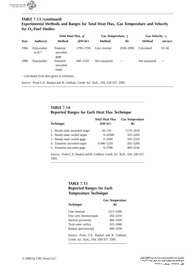
TABLE 7.13 (continued)
1984 Fairweather et al.27
Transient uncooled gage
1700–3700 Line reversal 2930–2990 Calculated 35–38
1986 Rauenzahn5 Transient uncooled target
645–1210 Not measured — Not measured —
a Calculated from data given in reference.
Source: From C.E. Baukal and B. Gebhart, Comb. Sci. Tech., 104, 339-357, 1995.
TABLE 7.14Reported Ranges for Each Heat Flux Technique
Total Heat Flux Gas TemperatureTechnique (kW/m2) (K)
1. Steady-state uncooled target 20–130 1179–16592. Steady-state cooled target 0–41000 323–32003. Steady-state cooled gage 0–3500 293–23504. Transient uncooled target 0.086–1210 292–32005. Transient uncooled gage 0–3700 400–3144
Source: From C.E. Baukal and B. Gebhart, Comb. Sci. Tech., 104, 339-357, 1995.
TABLE 7.15Reported Ranges for Each Temperature Technique
Gas TemperatureTechnique (K)
Line reversal 1213–3200Fine wire thermocouple 292–2350Suction pyrometer 460–2020Twin sonic orifice 323–3060Raman spectroscopy 600–3200
Source: From C.E. Baukal and B. Gebhart, Comb. Sci. Tech., 104, 339-357, 1995.
Experimental Methods and Ranges for Total Heat Flux, Gas Temperature and Velocity for O2 /Fuel Studies
Total Heat Flux, q″ Gas Temperature, tj Gas Velocity, vj
Year Author(s) Method (kW/m2) Method (K) Method (m/sec)
© 2000 by CRC Press LLC

TABLE 7.16
Line Reversal Measurements
Seeding Comparison Light SourceMax. tj
(K) Ref.
Sodium Not given 3200 Woodruff & Giedt, 196622
Sodium Tungsten filament 2100 Hargrave & Kilham, 198441
(cf. Hargrave, 198455)Sodium Tungsten filament 2260 Davies, 196534
Sodium Tungsten filament 2925 Kilham & Purvis, 197139
Sodium Tungsten filament 3144 Conolly & Davies, 19723
Sodium Xenon arc 2925 Kilham & Purvis, 197857
Sodium carbonate Carbon arc 2750 Fells & Harker, 196880
Sodium chloride Tungsten filament 1633 Kilham, 194913
Sodium chloride Tungsten filament 2990 Fairweather et al., 198427,40
Sodium chloride Xenon arc 2996 Nawaz, 197326
Source: From C.E. Baukal and B. Gebhart, Comb. Sci. Tech., 104, 339-357, 1995.
TABLE 7.17Fine Wire Thermocouple Measurements
T/C Alloys T/C Type CoatingMax. tj
(K) O.D. (mm) Ref.
Chromel/alumel K None Not given Not given Hustad et al., 19926
None 1700 Not given Hustad et al., 199116,17
Iron/constantan J Teflon 419 0.13 Veldman et al., 197542
Pt/Pt-Rh None 1720 0.1 Kataoka et al., 198429
None 1923 0.1 Buhr et al., 197366
Al2O3 Not given 0.1 Kremer et al., 197421
Pt/Pt-10%Rh S None 1500 0.05 You, 19857
None 1659 0.061–0.193 Jackson & Kilham, 195614
Pt/Pt-10%Rh & Pt-30%Rh/Pt-6%Rh
S, B Yt2O3 /BeO 2100 0.05–0.18 Hoogendoorn et al., 197852
Yt2O3 /BeO 2100 0.05–0.18 Popiel et al., 198053
Yt2O3 /BeO 2130 0.05–0.18 van der Meer, 199154
Pt/Pt-13%Rh R None Not given Not given Hargrave & Kilham, 198441
(cf. Hargrave, 198455)None 2165 0.5 Horsley et al., 198246
None 2350 0.24 Hargrave et al., 198774
SiO2 1450 0.127 Cookson & Kilham, 196735
SiO2 1910 0.127 Kilham & Dunham, 196749
SiO2 2200 0.127 Milson & Chigier, 19739
Pt-30%Rh/Pt-6%Rh B None Not given 0.3 Shorin & Pechurkin, 196820
Not given None 1600 Not given Matsuo et al., 197830
Source: From C.E. Baukal and B. Gebhart, Comb. Sci. Tech., 104, 339-357, 1995.
© 2000 by CRC Press LLC

TABLE 7.18
7.3.1 EQUATION PARAMETERS
The thermophysical properties and the stagnation velocity gradient have been used in all of the semianalytical solutions. Many methods have been used to calculate these parameters. Those methods are discussed here, prior to presenting the semianalytical solutions.
Pitot Measurements
Probe Type Ren
max. tj
(K) Coolant Materialo.d.
(mm) Ref.
Pitot tube Laminar 3200 Water Not given Not given Woodruff & Giedt, 196622
50–500 2200 Water Copper 3.6 Conolly & Davies, 19723
200–3600 1700 Not given Not given Not given Hustad et al., 199116,17
857–2000 1720 None Quartz 1.4 Kataoka et al., 198429
1050, 1860 2100 Water Tantalum 1.2 Hoogendoorn et al., 197852; Popiel et al., 198053
Turbulent 2020 Not given Not given Not given Smith & Lowes, 197437
Turbulent 1600 Not given Not given Not given Matsuo et al., 197830
4800–270,000 1950 Not given Not given Not given Beér & Chigier, 196823
Not given 3060 Water Tantalum 12 Rajani et al., 197838
Pitot-static 70, 356 1500 Not given Not given Not given You, 19857
1500–19,000 Not given None Alundum 1.8 Shorin & Pechurkin, 196820
Not given 2800 Water Not given Not given Ivernel & Vernotte, 197928
5-Hole Turbulent 1950 Not given Not given 8 Vizioz & Lowes, 197125
Turbulent 2020 Not given Not given Not given Smith & Lowes, 197437
Not given 3060 Water Tantalum 12 Rajani et al., 197838
Source: From C.E. Baukal and B. Gebhart, Comb. Sci. Tech., 104, 339-357, 1995.
TABLE 7.19Analyzers Used to Measure Gas Compositions
Ref. CH4 CO CO2 H H2 H2O N2 NO NO2 O2 OH
Buhr, 196985 GC GC GC GC GC GCConolly, 197150 Calc.Vizioz & Lowes, 197125 GC GC GC GC GC GCNawaz, 197326 GC GC GC Calc. GC GC GC LASmith & Lowes, 197437 GC GC GC GC GCRajani et al., 197838 IR IR CL CL Para.Ivernel & Vernotte, 197928 GC GC GC GC GCYou, 19857 GC GC GC GC GC GC GCPosillico, 198648 RS RS RS
Note: CL = chemiluminescent; GC = gas chromatograph; IR = nondispersive infrared; LA = line absorption; Para. = paramagnetic; and RS = Raman spectroscopy.
Source: From C.E. Baukal and B. Gebhart, Comb. Sci. Tech., 104, 339-357, 1995.
© 2000 by CRC Press LLC

7.3.1.1 Thermophysical Properties
These include the viscosity, density, thermal conductivity, Lewis number, and the enthalpy of the gaseous combustion products — all of which are temperature dependent (see Chapter 2). The temperature of the combustion products varies with the oxygen enrichment ratio, Ω. For stoichio-metric C3H8 flames, Chen (1972)62 showed how the properties vary as a function of Ω. Various methods have been used to evaluate the thermophysical properties. These methods are discussed below. The nomenclature is shown in Figure 7.16.
In every semianalytical solution, the gas temperature at the edge of the stagnation zone, te, has been used to evaluate some of the properties:
pe = p(te) (7.1)
where p is the property being evaluated. The wall temperature at the stagnation point of the target, tw, has also been used in every solution:
pw = p(tw) (7.2)
Many studies3,27,41,45,57 have used a weighted average, over the temperature range between the edge and the wall temperatures, as
(7.3)
The film, that is the mean temperature, between the edge and the wall temperatures has commonly been used:28,39,46,49
(7.4)
The reference temperature63 has been used in several solutions:52-54
(7.5)
where
(7.6)
For low-speed flows, trec Ý te, so pref Ý—p. Table 7.21 shows sample calculations, using the various
methods, for the thermal conductivity of the combustion products.64
FIGURE 7.15 Stagnation flow around a hemi-nosed, axisymmetric, body of revolution. (From C.E. Baukal and B. Gebhart, Int. J. Heat Fluid Flow, 39(14), 2989-3002, 1996.)
ppdt
t tw
e
e w
=−
∫
p pt te w=
−⎛⎝
⎞⎠2
p p t t t t te w e eref rec= + −( ) + −( ) 0 5 0 22. .
t tv
cee e
pe
rec = +2 0 5
2
Pr .
© 2000 by CRC Press LLC

TABLE 7.20
db
(mm)v
(m/s)tj
(K) Ref.
2.6–59.8 Not measured Not measured Hemeson et al., 198445
ot given Up to 50 Up to 2130 van der Meer, 199154
.6 diam. Not measured 1643–2165 Horsley et al., 198246
52 x 152 40–49 2755–2925 Kilham & Purvis, 197857
4 Not measured 1360–1450 Cookson & Kilham, 196335
2.2 Not measured 1624–1910 Kilham & Dunham, 196749
2.7 Not given9–17
22002543–3144
Conolly & Davies,19723
2 2–3 1900–2100 Hargrave & Kilham, 198441
0–150 Not measured Not measured Hemeson et al.,198445
.5 Not given 2600–27632795–2996
Nawaz,197326
.5 32–3635–38
2710–27602930–2990
Fairweather et al.,198427
.5 21–32 2755–2925 Kilham & Purvis,197139
6 5–5111–66
1640–27502300–2800
Ivernel & Vernotte, 197928
Experimental Studies Using Semianalytical Solutions
Target Oxidizer Ren φ Fuel βs
Cylinder Air 12600 1.05 Natural gas 2ve/r0.5t 3Flat plate Air 1700-4250 1.0 Natural gas ve/db N
Air 7050-16200 1.05 Natural gas ve/r0.5t 5O2 489-549
551-6920.95-1.311.45-1.83
CH4
C3H8
ve/dj 1
Hemi-nosed cylinder
Air Laminara 0.5-0.63 H2 3ve/db 1
Air Laminara 0.7-1.3 CO 3ve/db 2AirO2
50-500 1.0 Natural gasCH4,C2H4,C3H8,CO,H2
3ve/db 1
Air 1200-10000 1.0 CH4 (2.67+0.0926Tu)ve/db 2Air 12600 1.05 Natural gas 3ve/r0.5t 5Air/O2
O2
Laminara 0.62-1.140.83-1.70
CH4 3ve/db 9
Air/O2
O2
Laminarb 0.84-1.140.83-1.70
CH4 3ve/db 9
O2 Laminarb 0.95-1.311.45-1.83
CH4
C3H8
3ve/db 9
Air/O2
O2
Not given 0.95 Natural gas 2.5ve/db 4
a Calculated from data in the reference.b According to the author.
Source: From C.E. Baukal and B. Gebhart, Int. J. Heat Mass Transfer, 39(14), 2989-3002, 1996.
© 2000 by CRC Press LLC

FIGURE 7.16 Flame impingement on a hemi-nosed cylinder. (From C.E. Baukal and B. Gebhart, Int. J. Heat Mass Transfer, 39(14), 2989-3002, 1996.)
TABLE 7.21Thermal Conductivities for the Equilibrium Combustion Products for Stoichiometric CH4 Flames, Calculated Using Reference 64
Oxidizer
Parameter Units Air O2
tAFT K 2220 3054tw K 400 400te K 2000 2800
K 1200 1600trec K 2000.6 2800.1tref K 1200.1 1600.0kw W/m-K 0.0297 0.1546ke W/m-K 0.1693 1.6818
W/m-K 0.0860 0.1546W/m-K 0.0884 0.3288
kref W/m-K 0.0860 0.1546
Note: ve assumed to be 50 m/sec.
Source: From C.E. Baukal and B. Gebhart, Int. J. Heat
Mass Transfer, 39(14), 2989-3002, 1996.
© 2000 by CRC Press LLC
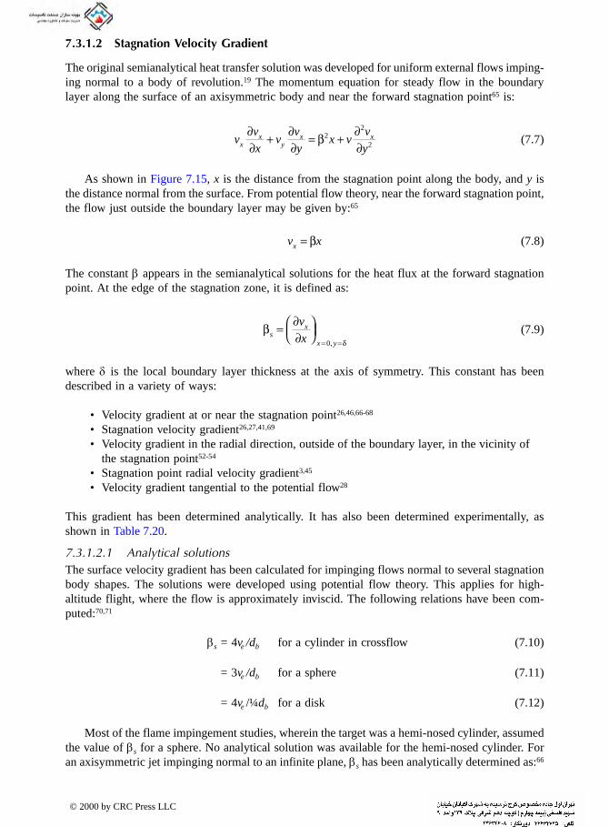
7.3.1.2 Stagnation Velocity Gradient
The original semianalytical heat transfer solution was developed for uniform external flows imping-
ing normal to a body of revolution.19 The momentum equation for steady flow in the boundary layer along the surface of an axisymmetric body and near the forward stagnation point65 is:
(7.7)
As shown in Figure 7.15, x is the distance from the stagnation point along the body, and y is the distance normal from the surface. From potential flow theory, near the forward stagnation point, the flow just outside the boundary layer may be given by:65
(7.8)
The constant β appears in the semianalytical solutions for the heat flux at the forward stagnation point. At the edge of the stagnation zone, it is defined as:
(7.9)
where δ is the local boundary layer thickness at the axis of symmetry. This constant has been described in a variety of ways:
• Velocity gradient at or near the stagnation point26,46,66-68
• Stagnation velocity gradient26,27,41,69
• Velocity gradient in the radial direction, outside of the boundary layer, in the vicinity of the stagnation point52-54
• Stagnation point radial velocity gradient3,45
• Velocity gradient tangential to the potential flow28
This gradient has been determined analytically. It has also been determined experimentally, as shown in Table 7.20.
7.3.1.2.1 Analytical solutionsThe surface velocity gradient has been calculated for impinging flows normal to several stagnation body shapes. The solutions were developed using potential flow theory. This applies for high-altitude flight, where the flow is approximately inviscid. The following relations have been com-puted:70,71
βs = 4ve /db for a cylinder in crossflow (7.10)
= 3ve /db for a sphere (7.11)
= 4ve /¼db for a disk (7.12)
Most of the flame impingement studies, wherein the target was a hemi-nosed cylinder, assumed the value of βs for a sphere. No analytical solution was available for the hemi-nosed cylinder. For an axisymmetric jet impinging normal to an infinite plane, βs has been analytically determined as:66
vv
xv
v
yx v
v
yxx
yx x∂
∂+ ∂
∂= + ∂
∂β2
2
2
v xx = β
βδ
sx
x y
v
x= ∂
∂⎛⎝⎜
⎞⎠⎟ = =0,
© 2000 by CRC Press LLC

(7.13)βs
e
j
v
d= π3
16
where dj is the diameter of the jet at the edge of the stagnation zone (see Figure 7.16). As shown in Figure 7.15, the external velocity far from the body of revolution, v×, is uniform. In Equations 7.10 to 7.13, the velocity at the edge of the boundary layer, ve, is equal to v×. For flame impingement, the external flow is generally not uniform. This is especially true if the target is large compared to the flame width. Therefore, ve is commonly a function of the axial distance between the burner and the target, L. Then, for impinging flames, ve = ve(x = 0, y = δ).
7.3.1.2.2 Empirical correlationsIn one study,46 βs was experimentally determined as a function of r0.5t. This is the radius at which the measured gas temperature is halfway between the maximum and the ambient, at a given axial location (see Figure 7.17):
(7.14)
In a related study,45 βs was determined for flames impinging normal to a cylinder, a hemi-nosed cylinder, and a flat plate, using the same type of formulation. The results are shown in Table 7.22. Two forms of βs were used. For the hemi-nosed cylinder, the calculated heat transfer, using βs1
, underpredicted the experimental measurements by up to 64%. The calculated heat transfer using βs2
only underpredicted the data by, at most, 29%. It overpredicted the data by up to 54%. Hargrave and Kilham (1984)41 determined βs as a function of turbulence intensity, Tu. For laminar flow (Tu = 0), βs = 2.67ve /db . This is slightly lower than the value of βs used in most of the hemi-nosed cylinder studies. In later studies, Hargrave and co-workers measured βs for heated air impinging normal to a cylinder72 and parallel to a hemi-nosed cylinder.73 For the cylinder, βs was empirically determined as βs = 3.85 + 4.90Tu. For the hemi-nosed cylinder, βs was empirically determined as βs = 2.67 + 9.62Tu. These relations were then used in subsequent flame impingement studies.74,75 In those studies, empirical — not semianalytical — heat transfer equations were determined. Therefore, those equations have not been included here. Van der Meer showed (1991) that βs = ve/db for disks applies within a distance of about five nozzle diameters from the burner outlet.54
FIGURE 7.17 Gas temperature profiles in a flame jet. (From C.E. Baukal and B. Gebhart, Int. J. Heat Mass Transfer, 39(14), 2989-3002, 1996.)
t t
t tr t0 5 0 5.
max
.−−
=∞
∞
© 2000 by CRC Press LLC
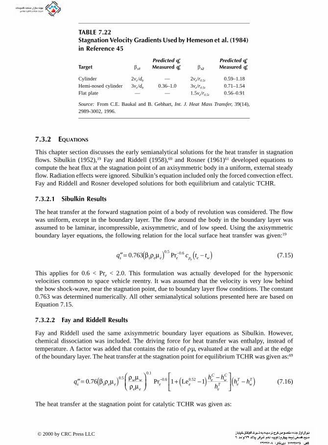
TABLE 7.22
7.3.2 EQUATIONS
This chapter section discusses the early semianalytical solutions for the heat transfer in stagnation flows. Sibulkin (1952),19 Fay and Riddell (1958),69 and Rosner (1961)61 developed equations to compute the heat flux at the stagnation point of an axisymmetric body in a uniform, external steady flow. Radiation effects were ignored. Sibulkin’s equation included only the forced convection effect. Fay and Riddell and Rosner developed solutions for both equilibrium and catalytic TCHR.
7.3.2.1 Sibulkin Results
The heat transfer at the forward stagnation point of a body of revolution was considered. The flow was uniform, except in the boundary layer. The flow around the body in the boundary layer was assumed to be laminar, incompressible, axisymmetric, and of low speed. Using the axisymmetric boundary layer equations, the following relation for the local surface heat transfer was given:19
(7.15)
This applies for 0.6 < Pre < 2.0. This formulation was actually developed for the hypersonic velocities common to space vehicle reentry. It was assumed that the velocity is very low behind the bow shock-wave, near the stagnation point, due to boundary layer flow conditions. The constant 0.763 was determined numerically. All other semianalytical solutions presented here are based on Equation 7.15.
7.3.2.2 Fay and Riddell Results
Fay and Riddell used the same axisymmetric boundary layer equations as Sibulkin. However, chemical dissociation was included. The driving force for heat transfer was enthalpy, instead of temperature. A factor was added that contains the ratio of ρµ, evaluated at the wall and at the edge of the boundary layer. The heat transfer at the stagnation point for equilibrium TCHR was given as:69
(7.16)
The heat transfer at the stagnation point for catalytic TCHR was given as:
Stagnation Velocity Gradients Used by Hemeson et al. (1984) in Reference 45
Target βs1
Predicted q″sMeasured q″s βs2
Predicted q″sMeasured q″s
Cylinder 2ve /db — 2ve/r0.5t 0.59–1.18Hemi-nosed cylinder 3ve /db 0.36–1.0 3ve/r0.5t 0.71–1.54Flat plate — — 1.5ve/r0.5t 0.56–0.91
Source: From C.E. Baukal and B. Gebhart, Int. J. Heat Mass Transfer, 39(14), 2989-3002, 1996.
′′= µ( ) −( )−q c t ts s e e e p e we0 763
0 5 0 6. Pr. .β ρ
′′= µ( ) µµ
⎛⎝⎜
⎞⎠⎟
+ −( ) −⎡
⎣⎢
⎤
⎦⎥ −( )−q
h h
hh hs s e e
w w
e ee e
eC
wC
eT e
TwT0 76 1 1
0 50 1
0 6 0 52. Pr.
.
. .β ρ ρρ
Le
© 2000 by CRC Press LLC

(7.17)′′= µ( ) µ⎛⎜
⎞⎟ + −( ) −⎡
⎢⎤⎥ −( )−q
h hh hs s e e
w we e
eC
wC
T eT
wT0 76 1 1
0 50 1
0 6 0 63. Pr.
.
. .β ρ ρLe
The only difference between the equations is the exponent of the Lewis number, Lee.
7.3.2.3 Rosner Results
In this formulation, the boundary layer equations were not solved directly, as had been done by Sibulkin and by Fay and Riddell. Instead, Fay and Riddell’s equations were modified to include the effects of chemical dissociation. The resulting equation was then the sum of a forced convection term from Sibulkin and a diffusion-chemical reaction term. Two different forms of the solution were given, depending on the nature of the thermochemical heat release.61 For equilibrium TCHR, the following form was recommended:
(7.18)
For catalytic TCHR, the recommended form was:
(7.19)
For equilibrium TCHR, Equation 7.18 differs significantly from that recommended by Fay and Riddell in Equation 7.16. For catalytic TCHR, Equation 7.19 is similar to that recommended in Equation 7.17. It has commonly been assumed that the driving force for energy transport is the total enthalpy difference across the boundary layer. Rosner noted that this is a common miscon-ception. It applies only for Lee = 1, since the terms inside the square brackets above also contain the total and chemical enthalpy differences across the boundary layer. For Lee = 1, Equations 7.18 and 7.19 yield the same result. For the O2 /H2 system considered by Rosner, the calculated heat flux was very similar using either equation, across a realistic range of values. The application was rocket motors. For that system, it was not important whether the TCHR was equilibrium or catalytic.
Rosner showed that the factor becomes more important as the target temperature approaches
the flame temperature (tw /te → 1). In that case, assuming Lee = 1 may seriously underestimate the actual heat flux.
7.3.3 COMPARISONS WITH EXPERIMENTS
This chapter section discusses the impingement experiments in which the measured heat flux was compared to some form of a semianalytical solution. There have been two types of experiments. The first was for lower temperature flames. There, forced convection is the dominant mechanism. TCHR is negligible. The second type was for higher temperature flames. There, forced convection and TCHR are both important. Both types are further classified into laminar and turbulent flow regimes.
7.3.3.1 Forced Convection (Negligible TCHR)
This mechanism has been important in air/fuel flames. In some studies,3,41,45 the driving potential was taken as (hT
e – hTw ). For air/fuel flames, this is essentially the same as (hS
e – hSw ).
µ⎝ ⎠ ⎣ ⎦he e eρ
′′= µ( ) + −( ) −−
⎡
⎣⎢
⎤
⎦⎥ −( )−q
h h
h hh hs s e e e
eC
wC
eT
wT e
TwT0 763 1 1
0 5 0 6
0 6
. Pr. .
.
β ρ Lee
′′= µ( ) + −( ) −−
⎡
⎣⎢
⎤
⎦⎥ −( )−q
h h
h hh hs s e e e e
eC
wC
eT
wT e
TwT0 763 1 1
0 5 0 6 0 6. Pr. . .β ρ Le
h hh h
eC
wC
eT
wT
−−
© 2000 by CRC Press LLC
7.3.3.1.1 Laminar flowIn one study,3 a wide range of heat fluxes was calculated (convection with and without TCHR) for
several variations of Equations 7.15 to 7.19. The best agreement with the experimental data was for:
(7.20)
The maximum deviation between this relation and the experimental data was 4%. Horsley et al. (1982)46 recommended the following modification of Equation 7.15:
(7.21)
This applies to 7050 ð Ren ð 16200. These values of Ren are generally considered to be turbulent,56
although the flames were described as having a “laminar appearance.”
7.3.3.1.2 Turbulent flowHorsley also inserted metal grids into industrial burners to promote turbulence.46 A similar modi-fication of Equation 7.15 was determined as,
(7.22)
This also applies to 7050 ð Ren ð 16200. The burner was located at the axial position, L, that yielded the maximum surface heat flux. The heat flux for the “laminar” flames, given in Equation 7.21, is greater than the flux for the turbulent flames given in Equation 7.22. Hargrave and Kilham (1984)41 recommended the following relation:
(7.23)
It was shown that TCHR was not important. Therefore, all properties were evaluated at Le = 1. Equation 7.23 correlated with the experimental data to within 4%. Hemeson et al. (1984)45 used a wide variety of burner designs. A range of cylinder and hemi-nosed cylinder diameters were tested. An equation similar to Equation 7.23, was suggested:
(7.24)
It was found that the heat flux did not depend on the radius of curvature for the cylinder or for the hemi-nosed cylinder. The flux was dependent on the burner design. Van der Meer (1991)54 used linear regression to correlate the experimental heat flux data as:
(7.25)
where γ = turbulence enhancement factor. This was an experimentally determined function of (Tu Re0.5). It varied from 0.0 for Tu = 0, up to about 0.4 for Tu Re0.5 ≅ 30.
′′= µ( ) µµ
−( )−q h hs s e e
eeT
wT0 763
0 5 0 6. Pr
. .β ρ
′′= µ( ) −( )−q h hs s e
SwS1 67
0 5 0 6. Pr
. .β ρ
′′= µ( ) −( )−q h hs s e
SwS1 12
0 5 0 6. Pr
. .β ρ
′′= µ( ) −( )−q h hs s e
TwT0 763
0 5 0 6. Pr
. .β ρ
′′= µ( ) −( )−q h hs s e eT
wT0 763
0 5 0 6. Pr. .β ρ
′′= +( ) µ( ) −( )−q h hs s eS
wS1 0 763
0 5 0 6γ β ρ. Pr. .
ref ref ref
© 2000 by CRC Press LLC
7.3.3.2 Forced Convection with TCHR
The combination of forced convection and TCHR has been most important in O /fuel flames. The
2
total enthalpy difference has been used as the driving potential. Some of the equations also included the effect of Le. Figure 2.50 shows the importance of Le for O2 /CH4 flames, especially at high temperatures.
7.3.3.2.1 Laminar flowCookson and Kilham (1963)36 tested fuel-lean air/H2 flames. Kilham and Dunham (1967)49 tested fuel-lean to fuel-rich air/CO flames. A modified form of Equation 7.18 was used in both studies. This included the catalytic TCHR effects for multiple active species:
(7.26)
The surface catalytic efficiency, Φi, is a measure of the ability of the surface to act as a catalyst in a chemical reaction. A value of 0.0 means no radical species will catalytically react as a result of contacting the surface. A value of 1.0 means that all radical species will catalytically react upon contacting the surface. In Equation 7.26, a value of 1.0 was assumed. The actual value was not known. The quasi-equilibrium composition for air/H2 mixtures was calculated, with a range of assumed concentrations of OH molecules.35 The equilibrium components included H, H2, H2O, N2, O, O2, and OH. Using these concentrations and the above equation, the heat flux as a function of OH concentration was calculated. By equating the calculated flux with the measured flux, the theoretical OH mole fraction was estimated to be 1.7% for φ = 0.5 and 3% for φ = 0.63. The experimental and calculated values were in excellent agreement at the location in the flame where the atom concentrations (e.g., O) were negligible.76 In general, the calculated values were shown to be highly dependent on the H, H2, O, and OH concentrations. Those concentrations were not measured. Using Equation 7.26 and the measured total heat flux, the O concentration was estimated to be 2% by volume. Kilham and Purvis39,77 measured the total heat flux from mostly fuel-rich flames. The data were compared to three different equations, using the recommendation by Fay and Riddell69 for ρeµe. Only forced convection heat transfer was assumed in the first equation:
(7.27)
Equilibrium TCHR with no Le augmentation (Le = 1) was assumed in the second equation:
(7.28)
Equilibrium TCHR with Le augmentation (Le > 1) was assumed in the third equation:
(7.29)
Equation 7.29 is a form of Equation 7.26. Kilham showed that Equation 7.26 could be simplified by calculating Lee and (hC
e – hCw ), based only on H atom recombination. Equation 7.27 underpredicted
′′= µ( ) + −( ) −−
⎡
⎣⎢⎢
⎤
⎦⎥⎥
−( )− ∑qh h
h hh hs s e e i
i
n
ie iC
w iC
eT
wT e
TwT0 763 1 1
0 5 0 6 0 6. Pr
. . . , ,β ρ Φ Le
′′= µ( ) µµ
⎛⎝⎜
⎞⎠⎟
−( )−q h hs s e e
w w
e eeS
wS0 763
0 50 1
0 6. Pr
..
.β ρ ρρ
′′= µ( ) µµ
⎛⎝⎜
⎞⎠⎟
−( )−q h hs s e e
w w
e eeT
wT0 763
0 50 1
0 6. Pr
..
.β ρ ρρ
′′= µ( ) µµ
⎛⎝⎜
⎞⎠⎟
+ −( ) −−
⎡
⎣⎢
⎤
⎦⎥ −( )−
qh h
h hh hs s e e
w w
e ee
eC
wC
eT
wT e
TwT0 763 1 1
0 50 1
0 60 6
. Pr.
..
,, ,
.
β ρ ρρ
Le HH H
© 2000 by CRC Press LLC

the experimental data by 24% to 42%. Equation 7.28 underpredicted the data by 3% to 7%. Equation 7.29 overpredicted the data by 2% to 10%. Conolly and Davies (1972)3 used several
variations of Equations 7.15 to 7.20. A wide range of heat fluxes (forced convection with and without TCHR) were calculated. Equation 7.20 gave the best agreement with the experimental data. Nawaz (1973)26 tested air-O2 /CH4 (Ω = 0.46–0.61) and O2 /CH4 flames. Variations of Equations 7.27 to 7.29 were used. For nonreacting flow, the relation was given as:
(7.30)
For equilibrium TCHR with Le = 1, the relation was given as:
(7.31)
For equilibrium TCHR with Le > 1, the relation was given as:
(7.32)
The Lee was calculated as the weighted average between the flame temperature and 1600K (2400°F). Based on the experimental data, the flame was divided into two regions. The region closest to the burner was assumed to have radicals in excess of that predicted by thermodynamic equilibrium calculations. This is referred to as superequilibrium. All three equations seriously underpredicted the measured data in that region. The far region, at about L > 0.7, appeared to be in chemical equilibrium. In that region, Equation 7.30 underpredicted the data by 17% to 77%; Equation 7.31 underpredicted by 0.6% to 5.5%; and Equation 7.32 overpredicted by 1.0% to 3.5%. It was con-cluded that the flow was mixed TCHR. As in their earlier study,39 Kilham and Purvis (1978)57 used three different equations to simulate various flow conditions. However, the Fay and Riddell69
recommendation for ρeµe was not used. The properties were also evaluated differently. The following relation was given for nonreacting flows:
(7.33)
This underpredicted the experimental data by 17% to 33%. The relation given for equilibrium TCHR, where Lee = 1, was:
(7.34)
For the CH4 flames and φ > 1.12, this underpredicted the data by at most 2%. For 0.95 ð φ ð 1.12, it overpredicted the data by as much as 40%. For the C3H8 flames and 1.45 ð φ ð 1.83, it underpredicted the data by 1% to 40%. The relation given for equilibrium TCHR, with Lee > 1, was:
(7.35)
′′= µ( ) µµ
⎛⎝⎜
⎞⎠⎟
−( )q h hs s e ew w
e eeS
wS0 763
0 50 24
. Pr.
.
β ρ ρρ e
-0.6
′′= µ( ) µµ
⎛⎝⎜
⎞⎠⎟
−( )q h hs s e ew w
e eeT
wT0 763
0 50 24
. Pr.
.
β ρ ρρ e
-0.6
′′= µ( ) µµ
⎛⎝⎜
⎞⎠⎟
+ −( ) −−
⎡
⎣⎢
⎤
⎦⎥ −( )q
h h
h hh hs s e e
w w
e ee
eC
wC
eT
wT e
TwT0 763 1 1
0 50 24
. Pr.
.
,, ,β ρ ρ
ρ e-0.6
HH HLe
′′= µ( ) −( )−q h hs s e eS
wS0 763
0 5 0 6. Pr. .β ρ
′′= µ( ) −( )−q h hs s e eT
wT0 763
0 5 0 6. Pr. .β ρ
′′= µ( ) + −( ) −−
⎡
⎣⎢
⎤
⎦⎥ −( )−q
h h
h hh hs s e e
eC
wC
eT
wT e
TwT0 763 1 1
0 5 0 6. Pr. .
,, ,β ρ Le HH H
© 2000 by CRC Press LLC

This overpredicted the data for both types of flames by as much as 48%. Fairweather et al. (1984)27
tested air-O2 /CH4 (Ω = 0.46–0.61) and O2 /CH4 flames. A modification of Equation 7.24 was used:
(7.36)
This was an upper limit when Le > 1. Equation 7.34 was used as a lower limit when Le = 1. For L > 0.8, Equation 7.34 underpredicted the data by up to 4%. Equation 7.36 overpredicted the data by up to 3%. For L < 0.8, Equations 7.34 and 7.35 underpredicted the data by up to 40%. The experimental data generally fell between these two limits, except near the reaction zone. There, all predictions severely underestimated the heat flux, compared to the measurements. It was determined that the inclusion of only H atom reactions was a good approximation to including all possible radical reactions.
7.3.3.2.2 Turbulent flowIvernel and Vernotte (1979)28 tested air-O2 /natural gas (Ω = 0.25–0.90) and O2 /natural gas flames. Although the flow regime was not specified, it appears to have been turbulent, based on a comparison with other studies.56 A variation of Equation 7.15 was used:
(7.37)
This differs from the other semianalytical solutions because most of the properties are evaluated at the wall temperature. Equation 7.37 overpredicted the experimental data by up to 68%.
7.3.4 SAMPLE CALCULATIONS
Sample calculations are given here to compare the predicted heat flux, using the semianalytical equations, with experimental measurements. The hemi-nosed cylinder is chosen as the target geometry since it was used in 9 of the 12 studies. Also, CH4 is chosen as the fuel since it was used in 10 of the 12 studies, either directly as methane or indirectly as natural gas. In all of these studies, the flame was at or near stoichiometric conditions. The first set of calculations is for a stoichiometric air/CH4 flame. This simulates forced convection without TCHR. Both laminar and turbulent con-ditions are modeled. The second set of calculations is for a stoichiometric O2 /CH4 flame. This has been chosen to simulate forced convection with TCHR. Only laminar flames have been considered. This is due to the lack of both correlations and measurements for turbulent flames with TCHR. Tables 7.23 to 7.25 show the comparison between the measured and the computed heat fluxes for the flames that have been modeled. The first section in each table lists the values for the important parameters, such as db, that are used in the computations. The measured heat flux is given next. Finally, the predictions are given in order of increasing heat flux.
7.3.4.1 Laminar Flames Without TCHR
Table 7.23 shows the measured and calculated heat fluxes for a laminar flame without TCHR. The measured heat flux by Hargrave and Kilham (1984)41 was from one set of tests at Ren = 2000. The rest of those tests were done under turbulent flow conditions. Those results are discussed in the next section. As expected, the correlation by Conolly and Davies (1972)3 in Equation 7.20, closely matches their own experimental data. The other three correlations significantly overpredict that data. The heat flux measurements by Hargrave and Kilham varied widely with L. The fluxes calculated using Equations 7.15 and 7.25 are within the measured range. Equation 7.21 overpredicts
′′= µ( ) −( )−q h hs s e
TwT0 763
0 5 0 6. Pr
. .β ρ
′′= µ( ) −( )q h hs s w ww
eT
wT0 763
0 50 4
.PrPr
..
β ρ
© 2000 by CRC Press LLC

TABLE 7.23
the Conolly and Davies experimental data by 360%. It overpredicts the Hargrave and Kilham data by up to 220%. Heat flux measurements from laminar air/fuel flames to hemi-nosed cylinders with a variety of diameters56 have ranged from 73 to 460 kW/m2 (23,000 to 146,000 Btu/hr-ft2). The results using Equations 7.15, 7.21, and 7.25 for the Conolly and Davies3 conditions exceed that range.
7.3.4.2 Turbulent Flames Without TCHR
The results for this case are shown in Table 7.24. The heat flux measured by Hargrave and Kilham, varied widely with turbulence intensity, Tu, and with axial position, L. The predicted heat flux values, using Equations 7.22 and 7.25, are within the measured range. Hargrave and Kilham recommended the relation given in Equation 7.23. It underpredicts their own experimental data by 7% to 66%. Heat flux measurements from turbulent air/fuel flames to hemi-nosed cylinders of various diameters have ranged from 100 to 580 kW/m2 (32,000 to 180,000 Btu/hr-ft2). The calcu-lations in Table 7.24 are all within that range.
Heat Flux for Laminar Flames Without TCHR
Parameter Units Conolly & Davies (1972)3 Hargrave & Kilham (1984)41
βs sec–1 3ve /db 2.67ve /db
db mm 12.7 22ve m/sec 11 2.5tw K 400 393te K 2200 2000q″s , measured kW/m2 265 110–210q″s , Eq. 7.20 kW/m2 272 81q″s , Eq. 7.25, γ = 0 kW/m2 590 163q″s , Eq. 7.15 kW/m2 642 157q″s , Eq. 7.21 kW/m2 1225 356
Source: From C.E. Baukal and B. Gebhart, Int. J. Heat Mass Transfer, 39(14), 2989-3002, 1996.
TABLE 7.24Heat Flux for Turbulent Flames Without TCHR
Parameter Units Hargrave & Kilham (1984)41
βs, Tu = 0.2 sec–1 2.7ve /db
db mm 22ve m/sec 2.5tw K 393te K 2000q″s , measured kW/m2 150– 410q″s , Eq. 7.23 kW/m2 139q″s , Eq. 7.24 kW/m2 146q″s , Eq. 7.25, γ = 0.4 kW/m2 229q″s , Eq. 7.22 kW/m2 240
Source: From C.E. Baukal and B. Gebhart, Int. J. Heat Mass
Transfer, 39(14), 2989-3002, 1996.
© 2000 by CRC Press LLC

TABLE 7.25
7.3.4.3 Laminar Flames with TCHR
The results for this case are given in Table 7.25. There is a wide variation in the predicted flux. However, most of the predictions that incorporate TCHR closely approximate the measurements. As expected, the correlations given in Equations 7.28, 7.30, and 7.33, for nonreacting flow signif-icantly underpredict the data. The lowest heat flux prediction is for Equation 7.27. It underpredicts the measurements by 44 to 58%. This is because the sensible, not the total, enthalpy difference was used as the driving force. The highest predictions are for Equation 7.35. It overpredicts the measurements by 24% to 67%. The results using Equations 7.32, 7.34, and 7.35 exceeded the range for the Nawaz26 and Fairweather27 measurements.
The heat flux calculated using Fay and Riddell’s relation for equilibrium TCHR in Equation 7.16, was lower than that for catalytic TCHR in Equation 7.17. However, the predicted heat flux using Rosner’s relation for equilibrium TCHR in Equation 7.18 was higher than that for catalytic TCHR in Equation 7.19. Therefore, no trend in the predictions is apparent when comparing catalytic and equilibrium TCHR. Heat flux measurements from laminar O2 /fuel flames to hemi-nosed cylinders of various diameters have ranged from 410 to 3700 kW/m2 (130,000 to 1.2 × 10⁶ Btu/hr-ft2).56
7.3.5 SUMMARY
Twelve flame impingement experimental studies were reviewed here. In those studies, the measured heat flux was compared against one or more semianalytical solutions. Cylindrical, flat plate, and
Heat Flux for Laminar Flames with TCHR
ParameterTCHR Type Units Kilham & Purvis, 197139
Nawaz, 197326; Fairweather et al., 198427
βs sec–1 3ve /db 3ve /db
db mm 9.5 9.5ve m/sec 27 37tw K 380 360te K 2800 2900q″s , measured kW/m2 2530 2700–3640q″s , Eq. 7.20 kW/m2 1163 1520q″s , Eq. 7.27 kW/m2 1240 1520q″s , Eq. 7.30 kW/m2 1630 2030q″s , Eq. 7.33 kW/m2 1910 2440q″s , Eq. 7.28 kW/m2 1950 2580q″s , Eq. 7.26 Catalytic kW/m2 2020 2690q″s , Eq. 7.29 Equil. kW/m2 2100 2800q″s , Eq. 7.36 kW/m2 2340 3180q″s , Eq. 7.19 Catalytic kW/m2 2510 3400q″s , Eq. 7.18 Equil. kW/m2 2510 3410q″s , Eq. 7.31 kW/m2 2550 3450q″s , Eq. 7.16 Equil. kW/m2 2560 3490q″s , Eq. 7.17 Catalytic kW/m2 2600 3540q″s , Eq. 7.32 Equil. kW/m2 2740 3760q″s , Eq. 7.34 kW/m2 3000 4140q″s , Eq. 7.35 Equil. kW/m2 3230 4510
Source: From C.E. Baukal and B. Gebhart, Int. J. Heat Mass Transfer, 39(14), 2989-3002, 1996.
© 2000 by CRC Press LLC

hemi-nosed cylindrical targets were used in 1, 3, and 9 studies, respectively. Note that Hemeson et al. (1984)45 used both a cylindrical target and a hemi-nosed cylinder target. Laminar flames have
been used more often than turbulent flames.
Catalytic TCHR has been considered in only two studies,35,49 as given in Equation 7.26. An uncertainty is the lack of information on the surface catalytic efficiency, Φ, for given target materials. None of the studies compared the experimental results to both equilibrium and catalytic TCHR solutions. No semianalytical solutions have been suggested for mixed TCHR.
Sample calculations for laminar and turbulent flows without TCHR, and laminar flows with TCHR, generally showed good agreement with the experimental data. However, in one case, the prediction was nearly 5 times the experimental data. Therefore, caution must be used in the absence of any experimental data.
There are many possible explanations for the discrepancies between the predictions and the experimental data. It has been assumed that the experimental data are reliable. However, none of the studies gave an estimate of the uncertainty in the measurements. In most cases, a complete set of data has not been given for a specific heat flux measurement. Commonly, a range of values or an average value for a particular variable has been given. For example, Hargrave and Kilham (1984)41
reported gas temperatures ranging from 1900K to 2100K (3000°F to 3300°F). No specific relation-ship between those temperatures and the reported heat fluxes was given. In the sample calculations, an average value of 2000K (3100°F) was used. Another possible source of error in the calculations is the choice of βs. In most cases, Equation 7.11 for a sphere has been used, in the absence of an equation for a hemi-nosed cylinder. Also, the gases have been assumed to be at equilibrium condi-tions. In many cases, this is a reasonable assumption. However, Cookson and Kilham (1963)36 and Kilham and Dunham (1967)49 showed that the gases in the region closest to their burner were not in equilibrium. This could dramatically affect the properties used in the calculations.
For high-temperature flames, where dissociation is important, the TCHR effects must be included. Otherwise, the predictions will significantly underpredict the data. Fay and Riddell69 and Rosner61 have developed solutions for both equilibrium and catalytic TCHR. However, the sample calculations in Table 7.25 showed that the results are nearly the same for either type of TCHR. Further work should determine if that would be true over a wider range of conditions.
7.4 EMPIRICAL HEAT TRANSFER CORRELATIONS
Empirical heat transfer correlations for impinging flame jets have been generally given in two forms.78 The first is the Nusselt number, which is a dimensionless heat transfer coefficient. In the studies considered here, it has appeared as:
Nu Ý a Prb Rec
where a, b, and c are constants. The second form has been directly in terms of the heat flux, q″. These two forms are related as follows:
q″ = (k/d)Nu ∆t
where k is the thermal conductivity of the fluid and d is a characteristic dimension.For consistency, most of the correlations given here are written in terms of q″. This makes it
easier to directly compare equations. Also, the driving force, or the potential for heat transfer, is explicitly given in the second form. In some correlations, this potential is the temperature difference. In others, it is the enthalpy difference. In the first form, the Nu formulation, the potential is not given explicitly. For the correlations converted from the first form to the second form (i.e., Nu to q″), the Nu relationship is shown inside curly brackets .
© 2000 by CRC Press LLC

This chapter section is arranged to aid the designer or researcher in finding the appropriate correlation for a specific set of conditions. The primary consideration is to ensure that the heat
transfer correlation applies to the chosen geometric configuration. The next consideration is the location on the target where the desired flux is to be calculated. This has typically been at a specific location, such as the stagnation point. This is referred to as a local heat flux. Correlations have also been determined for the average heat flux over a given portion of the target. Next, the correlations are arranged in terms of the heat transfer mechanism(s). These include convection, TCHR, radiation, and combinations of these. Finally, the correlations are arranged by the flow type (laminar or turbulent). In some studies (e.g., see Reference 27), correlations were given for both laminar and turbulent flows. However, in other studies, the flow type was not specified.
7.4.1 THERMOPHYSICAL PROPERTIES
The transport and thermodynamic properties used in the correlations presented below are discussed in this chapter section. These properties have been evaluated using several rules. These properties include, for example, the specific heat, thermal conductivity, enthalpy, and viscosity of the com-bustion products. The nomenclature is shown in Figure 7.16. The properties have been evaluated at the gas temperature at the edge of the stagnation zone and the boundary layer, te (Equation 7.1), at the wall temperature of the target, tw (Equation 7.2), at the weighted average over the temperature range between the edge of the stagnation zone and the wall temperatures (Equation 7.3), at the film temperature (Equation 7.4), and at the reference temperature (Equation 7.5). In addition, Beér and Chigier (1968)23 evaluated the properties at the maximum temperature measured at a given location in the flame jet:
pmax = p(tmax) (7.38)
Definitions of dimensionless quantities to be introduced below, such as Re, Nu, and Pr, will require specification of a characteristic length scale and characteristic transport properties. The transport properties will, in turn, require specification of the rule by which they are evaluated (e.g., use of a specific characteristic temperature of the material). When only transport properties (i.e., material temperature) are required, this will be indicated by a single subscript (e.g., Pre [i.e., Pr evaluated at te]). When both a characteristic length and a property temperature are required, these will be indicated by the first and second of two subscripts, respectively. For example, Ren,e is shorthand notation for:
For this example, the characteristic dimension is dn. That dimension is an important parameter in correlating the heat transfer. There are many possible lengths that can be used. The most common one has been the burner nozzle diameter, dn. Another has been the axial distance from the nozzle edge to the surface stagnation point, lj. For cylindrical and hemi-nosed cylindrical targets (see Figures 7.9 and 7.10), the diameter of the body, db, has been used. For plane targets, the distance along the surface, r, has also been used. Smith and Lowes (1974)37 used the width of the cooling channel in the target, lc . Kataoka et al. (1984)29 used the radius where the velocity was half the axial (r = 0) velocity, r1/2v .
7.4.2 FLAMES IMPINGING NORMAL TO A CYLINDER
This refers to flames impinging perpendicular to a cylinder, as in Figure 7.9, a cylinder in crossflow. The experimental conditions for previous studies using this geometry are given in Table 7.1. The table also shows which heat transfer mechanisms were correlated in those studies.
Re ,n e e e n ev d= µρ
© 2000 by CRC Press LLC

7.4.2.1 Local Convection Heat Transfer
7.4.2.1.1 Laminar and turbulent flows
Hustad and co-workers (1991)17 measured the radiation and the total heat fluxes for both laminar and turbulent flows. The radiation flux was also calculated. The convection heat transfer was calculated by subtracting the calculated radiation from the measured heat flux. Several correlations from the literature were tested for the convective portion of the heat transfer. The best match with the experimental convection at the stagnation point was the correlation from Zukauskas and Ziugzda (1985),79 assuming Tu = 0.02:
(7.39)
For a pure fuel jet, there may have been significant quantities of uncombusted species in the flame at the impingement point. Therefore, TCHR may have been important, but was not discussed by Hustad and co-workers. If TCHR was present, it would have been included with forced convection in Equation 7.39.
7.4.2.1.2 Turbulent flowsHargrave et al. (1987)75 studied the effects of turbulence. The following correlation was determined:
(7.40)
This correlation underpredicted the data by up to 14%.
7.4.2.2 Average Convection Heat Transfer
7.4.2.2.1 Laminar flowsIn related studies, Kilham (1949)13 and Jackson and Kilham (1956)14 measured the total and radiative heat fluxes. The convective heat transfer was calculated by subtracting the radiation from the total heat flux. Kilham studied air/CO flames. The convection was correlated by:
(7.41)
Jackson and Kilham studied air/H2, O2 /H2, and O2 /CO flames. The convection was correlated by:
(7.42)
Both equations were valid for 60 ð Reb ð 230. The constant multiplying Reb varied slightly in the two studies. McAdams’ (1954) correlation59 for this geometry, but for nonreacting jet impingement, had a multiplier of 0.47. In the O2 /H2 and O2 /CO flames used in Jackson and Kilham’s study, there may have been significant quantities of dissociated species. Therefore, TCHR may have been important, but was not discussed. If TCHR was present, it would have been included in Equation 7.42. However, a larger difference in Equations 7.41 and 7.42 would have been expected if TCHR was significant.
′′ =⎛⎝⎜
⎞⎠⎟
⎧⎨⎪
⎩⎪
⎫⎬⎪
⎭⎪−( )q
k
dt ts
e
bb e e
e
we w, ,
. . .
.
. Re PrPr
Prconv Tu0 41 0 6 0 35 0 15
0 25
′′ = +⎛
⎝⎜
⎞
⎠⎟ −
⎛
⎝⎜
⎞
⎠⎟
⎡
⎣⎢⎢
⎤
⎦⎥⎥
⎧⎨⎪
⎩⎪
⎫⎬⎪
⎭⎪−( )q
kd
t tsb
bb b
e w,
.. .
Re . .Re
.Re
conv
Tu Tu0 50 5 0 5 2
1 071 4 669100
7 388100
′′ = +( ) −( )qkd
t tbb
b e w,
. .Pr . . Reconv
0 3 0 520 35 0 47
′′ = +( ) −( )qkd
t tbb
b e w,
. .Pr . . Reconv
0 3 0 520 35 0 50
© 2000 by CRC Press LLC

7.4.2.2.2 Laminar and turbulent flowsHustad and co-workers (1991)17 measured the total heat flux. The radiation heat flux was assumed
to be uniformly distributed around the cylinder. The forced convection was calculated by subtracting the calculated radiation from the measured total heat flux. At a turbulence intensity of 2%, the best fit of the data was given by:
(7.43)
7.4.2.2.3 Flow type unspecifiedFells and Harker (1968)80 empirically determined:
(7.44)
for C3H8 flames. This correlated with the experimental data to within 10%. Davies (1979)18
calculated the forced convection heat transfer using an equation developed by Conolly and Davies (1972)3 for a water-cooled tube in crossflow:
(7.45)
7.4.2.3 Average Convection Heat Transfer with TCHR
7.4.2.3.1 Flow type unspecifiedDavies (1965)34 correlated heat flux data using an equation from McAdams (1954),59 assuming Pr = 0.7:
(7.46)
7.4.2.4 Average Radiation Heat Transfer
7.4.2.4.1 Laminar and turbulent flowsHustad and co-workers (1991)17 studied pure diffusion flames. The radiation from the CH4 flames was given as:
(7.47)
The radiation for the C3H8 flames was given as:
(7.48)
These were based on an analytical model of the flame as a radiating cylinder. The liftoff distance, xliftoff, is the length between the nozzle and the start of the flame. The length lj – xliftoff was termed the radiation height. For a conventional burner, xliftoff is zero since the flame is attached to the nozzle exit. The distances used in Equations 7.47 and 7.48 were in meters. In those studies, the fuel gas
′′ =⎛⎝⎜
⎞⎠⎟
⎧⎨⎪
⎩⎪
⎫⎬⎪
⎭⎪−( )q
k
dt tb
e
bb e e
e
we w, ,
. . .
.
. Re PrPr
Prconv Tu0 23 0 6 0 35 0 15
0 25
′′ = −( ) −( )qkd
l t tbb
j b e w,
.. . Reconv 0 573 0 0179
0 5
′′ = ( ) −( )q k d t tb b b e w,
. .. Pr Reconv 1 32
0 4 0 5
′′ = ( ) −( )q k d t tb b b e w,
.. Reconv+TCHR 0 615
0 466
′′ = + −( ) ( )q l xb j, . rad liftoff kW m5 3 9 2
′′ = + −( ) ( )q l xb j, . rad liftoff kW m19 7 8 2
© 2000 by CRC Press LLC

velocities at the nozzle outlet in terms of the Mach number were Ma Š 0.3. This equates to a minimum outlet velocity of 134 and 82 m/sec (440 and 270 ft/sec) for CH4 and C3H8, respectively.
The burning velocity in air for CH4 and C3H8 is 0.37 and 0.41 m/sec (1.2 and 1.35 ft/sec), respectively.81 Therefore, the flames were not attached to the burner because the exit velocities were much higher than the flame speed. This produced a so-called unattached or lifted flame. The flame starts where the local gas velocity is the same as the flame speed.
7.4.2.5 Maximum Convection and Radiation Heat Transfer
7.4.2.5.1 Turbulent flowsHustad et al. (1992)6 correlated their experimental data by:
(7.49)
based on a thermal input of qf = 60 to 1600 kW (200,000 to 5.5 × 10⁶ Btu/hr). The location of the maximum heat flux was at the center of the flame. For pure fuel jets, there may have been significant quantities of unburned fuel at the target impingement point. Therefore, TCHR may have been important. It would have been included in the above correlation.
7.4.3 FLAMES IMPINGING NORMAL TO A HEMI-NOSED CYLINDER
This pertains to cylinders whose axis is parallel to the flame, as shown in Figure 7.10. One end of the cylinder has a hemispherical nose. The flame impinges on that nose. Experimental conditions for these studies are given in Table 7.2.
7.4.3.1 Local Convection Heat Transfer
7.4.3.1.1 Laminar and turbulent flowsFairweather et al. (1984)27 correlated experimental data for laminar and turbulent flames. The correlations were modifications of empirical equations. These were derived for heat transfer from the stagnation point of heated spheres to turbulent air flows. Galloway and Sage (1968)82 recom-mended the following equations for nonreacting flows:
(7.50)
(7.51)
Fairweather used modifications of these equations to get:
(7.52)
Gostkowski and Costello (1970)83 recommended the following equation, also for nonreacting flows:
(7.53)
′′ = ( )q qfmax,conv+rad kW m10 0 3 2.
Nu Tu for Tu= ( ) <1 255 70000 5 0 0214. Re Re Re,
.,
.
,b e b e b e
Nu Tu for Tus e b e b e b e, ,.
,
.
,. Re Re Re= ( ) >1 128 70000 5 0 2838
′′ = ( ) −( )qv c
t ts b ee e p
b ee w
e, ,
.
,.. Re
Reconv Tu1 7430 0214
0 5
ρ
Nu Tu Tus ee
wb e e b e e
v
v,
.
, ,. . . . Re Pr Re Pr= +⎛⎝⎜
⎞⎠⎟
+ −( ) +[ ]⎧⎨⎪
⎩⎪
⎫⎬⎪
⎭⎪2 1 849 0 2122 0 1072 0 001317
0 16
1 2 1 6 1 2 1 3
© 2000 by CRC Press LLC

Fairweather recommended the following modification of Equation 7.53 for laminar and turbulent flames:
(7.54)
Both Equations 7.52 and 7.54 tended to overpredict the experimental data.
7.4.3.1.2 Turbulent flowsHargrave et al. (1987)75 recommended the following empirical correlation:
(7.55)
This underpredicted the data by up to 15% near the reaction zone. Agreement was very good further downstream.
7.4.3.2 Local Convection Heat Transfer with TCHR
7.4.3.2.1 Turbulent flowsIvernel and Vernotte (1979)28 determined:
(7.56)
This was valid for 1000 < Rerb ,w < 45000. Equation 7.56 correlated with the experimental data to within 10%. Although the flow conditions were not given, they are believed to have been turbulent. This is based on a comparison of the reported velocities with those of other studies (see Baukal and Gebhart, 199556). Radiation to the target was calculated. It was specifically excluded from the above correlation.
7.4.4 FLAMES IMPINGING NORMAL TO A PLANE SURFACE
This geometry is shown in Figure 7.11. The targets have included both disks and rectangular plates. The experimental conditions are given in Table 7.3.
7.4.4.1 Local Convection Heat Transfer
7.4.4.1.1 Laminar flowsIn related studies, Hoogendoorn et al. (1978)52 and Popiel et al. (1980)53 determined two empirical correlations for the heat transfer to the stagnation point. These were based on the axial distance between the target and the burner. The correlation for 2 ð L ð 5 was:
(7.57)
′′ =+
⎛⎝⎜
⎞⎠⎟
+ −( ) +[ ]
⎡
⎣
⎢⎢⎢⎢
⎤
⎦
⎥⎥⎥⎥
−( )−
q v c
v
v t ts e e p e b e e b e
e
w
e
e we, , ,
.
Pr Re.
Pr Re
. . . Pr
conv
Tu Tu
ρ
2 1 1849
0 2122 0 1072 0 001317
2 3 1 2
0 16
1 2
′′ = +⎛
⎝⎜
⎞
⎠⎟ −
⎛
⎝⎜
⎞
⎠⎟
⎡
⎣
⎢⎢
⎤
⎦
⎥⎥
⎧⎨⎪
⎩⎪
⎫⎬⎪
⎭⎪−( )q
kd
t tsb
bb b
e w,
.. .
Re . .Re
.Re
conv
Tu Tu0 50 5 0 5 2
0 993 5 465100
2 375100
′′ = −q
k
r
h h
csw
br w
eT
wT
pb
w
, ,
.. Re Prconv+TCHR 0 853
0 4
′′ = +( ) −q
k
d
h h
csn
neS
wS
p, ,
.. . Re Prconvref
ref0.5
refLref
0 65 0 084 0 4
© 2000 by CRC Press LLC
The correlation for L > 12 was:
(7.58)
Both correlations closely matched the data. For 5 < L ð 12, the data showed a peak for Nun. No correlation was given. A modified form of a semianalytical solution was also determined. It was a form of the Equation 7.15 recommended by Sibulkin.19 The modified correlation was:
(7.59)
valid for 8 ð L ð 20. This underpredicted the data by as much as 60%. This was believed to have been caused by the failure to include the effects of free jet turbulence. Another correlation was recommended that included those effects:
(7.60)
valid for L Š 8. This compared favorably with the data. For L Š 4, the maximum heat flux occurred at the stagnation point. For L = 2 and 3, the maximum flux occurred at about R = 0.5 and 0.2, respectively. Kataoka et al. (1984)29 studied an air-O2 /CH4 (Ω = 0.39) flame. The heat transfer to the stagnation point was correlated by:
(7.61)
r1/2v is the radius from the burner axis near the stagnation point where the velocity is 1/2 of the velocity along the axis of symmetry. This correlation is valid only for L > Xv with Xv correlated by:
(7.62)
In a subsequent study, Kataoka (1985)84 found that the maximum heat flux for the same flame occurred at L = Xv .
7.4.4.1.2 Turbulent flowsShorin and Pechurkin (1968)20 empirically determined:
(7.63)
This was valid for L ð Xv . The correlation matched the experimental data within 15%. Another correlation was given for the heat flux for L > Xv:
(7.64)
′′ = ( ) ⋅ −−qk
d
h h
csn
neS
wS
p, ,
.Re Prconvref
ref0.75
ref37 -1.8Lref
1 10 3 0 4
′′ = +( ) −−qk
d
h h
csn
neS
wS
p,
.,
.. Re Prconvref
ref0.5
refLref
2 37 1 0 5 0 4
′′ =+( )
+⎛
⎝⎜⎞
⎠⎟−
⎛
⎝⎜⎞
⎠⎟⎡
⎣⎢⎢
⎤
⎦⎥⎥
⎧⎨⎪
⎩⎪
⎫⎬⎪
⎭⎪
−q
k
d
h h
csn
n nn
eS
wS
p, .
,.
,.
,. ..
. . Re Prconvref ref ref
ref refL
TuRe TuRe
ref
2 371
2 22100
2 761000 5
0 5 0 5 2
0 5 0 4
′′ = −( ) −( )qk
rt ts
e
vr e e v e wv, ,. . .
. Re Prconv L X2
1 441 2
20 5 0 5 0 12
1 2
X Xv n n= ( )∞ =2 820 29
00 07. Re
.
,.ρ ρ
′′ = −( )qk
dt ts
e
nn e e e w, ,.. Re Prconv 4 04 0 2
Nu X L
Nu L X
L X
Ls e v
s e v
ev
,
,
..
< <( )<( ) =
−−( )14
0 80 36
2
© 2000 by CRC Press LLC

The local heat transfer, as a function of R, was correlated by:
(7.65)
for 0 < R/L < 0.9. Vizioz and Lowes (1971)25 investigated industrial-scale, air and oxygen-enriched air (Ω = 0.30) natural gas flames impinging on cooled flat plate targets located inside a furnace. Three different types of flames with various levels of swirl were tested. The data were correlated by:
(7.66)
In one set of tests, the surface temperature of a water-cooled steel flat plate was maintained below 373K (212°F). The convective heat flux as a function of radius from the stagnation point was:
(7.67)
In another set of tests, the surface temperature of an air-cooled refractory plate was maintained between 1280K and 1420K (1850°F and 2100°F). The convection correlation was:
(7.68)
The Prandtl number effect was included in the coefficients.In related studies, Buhr et al. (1969, 1973)66,85 and Kremer et al. (1974)21 determined the
following modification of Sibulkin’s equation:
(7.69)
This was valid for 17680 ð Ren ð 22700, 13 ð L ð 65. The experimental data was correlated within 9%. The peak flux was measured near the reaction zone. The heat flux showed a small linear decline with probe surface temperature over the range 320K to 1000K (120°F to 1300°F). Smith and Lowes (1974)37 determined the following empirical correlation:
(7.70)
where lc was the width of the cooling channels. The correlation was valid for 0 ð L ð 8.4. The fluid properties were taken, as for air, at the gas temperatures measured near the plate. The axial velocity at 10 cm (4 in.) from the plate was used to calculate the velocity in Ren.
Matsuo et al. (1978)30 determined the following correlation, for the heat flux to the stagnation point:
(7.71)
Another correlation was given for the heat flux as a function of the distance r from the stagnation point:
(7.72)
′′ =⎧⎨⎪
⎩⎪
⎫⎬⎪
⎭⎪−( )−
−( ) −q
k
re t tr
en e e
R
Le w
v
, ,. . .
. Re Prconv
L X
L3 22 0 4 0 36 3 62
′′ = ( ) −( )q k r t tr e r e e w, ,conv Nu
0 07 0 220 8. Re . Re,.
, ,r e r e r e< <Nu
0 035 0 1250 8. Re . Re,.
, ,r e r e r e< <Nu
′′ = −( )−q v h hs e e e eS
sS
,.. Prconv 0 0371 0 6 ρ
′′ = ( ) −( )q k l t ts e c l e e e wc, ,. .. Re Prconv 1 6 0 54 0 52
′′ = ( ) −( )q q t ts f e w,. ..conv L0 010353 0 936 1 032
′′ =⎛
⎝⎜
⎞
⎠⎟ −( )
⎛⎝⎜
⎞⎠⎟q q K K t ts f
re w,
...
conv L0 9391 2
6 3180 414
© 2000 by CRC Press LLC

where
(7.73)K r r7 2 31 903 10 3 89 10 0 985= − ⋅ + ⋅ +− −. . .
(7.74)
Equations 7.71 and 7.72 were valid for 5 ð L ð 9 and 148 ð qf ð 482. Equation 7.72 was valid for 0 < r ð 500, where r was in millimeters.
7.4.4.2 Local Convection Heat Transfer with TCHR
7.4.4.2.1 Laminar flowsAnderson and Stresino (1963)15 found that the heat flux decreased exponentially as R increased:
(7.75)
where q″s,conv + TCHR was measured and dj was the estimated flame diameter prior to impingement. Shorin and Pechurkin (1968)20 found for C3H8 + C4H10 flames that:
(7.76)
for L ð Xv . This correlated with the data to within 10%.
7.4.4.2.2 Turbulent flowsRauenzahn (1986)5 calculated the heat flux at the surface for the transient temperature field in a copper block. The assumed form of the surface flux distribution, after Anderson and Stresino,15 was:
(7.77)
r0 was termed the spreading radius for the heat flux distribution. From the reduction of the data, a ≅ 1. A transient inverse conduction analysis (see Gebhart, 199386) was used to calculate q″s,conv + TCHR
and q″r,conv + TCHR . For qf = 61 and 94 kW (210,000 and 320,000 Btu/hr) and L = 6 and 8, q″s,conv + TCHR
ranged from 645 to 1210 kW/m2 (205,000 to 384,000 Btu/hr-ft2), and r0 ranged from 7.3 to 9.8 cm (2.9 to 3.9 in.). The spreading radius generally decreased as L decreased and as qf increased. Unfortunately, no correlations were given for q″s,conv + TCHR and r0 in terms of L and qf . Therefore, the constants used in the above equation are expected to be dependent on the specific experimental conditions.
7.4.4.3 Average Convection Heat Transfer
7.4.4.3.1 Laminar flowsYou (1985)7 studied pure diffusion flames impinging on a plate. The fuel flow from the burner nozzle was laminar. However, the buoyant plume impinging on the plate was turbulent. It was found that the convective heat flux in the stagnation zone was essentially constant:
(7.78)
1
K r r r27 3 3 28 42 10 1 803 10 1 37 5 00= ⋅ − ⋅ + +−. . . .
′′ = ′′− −
q q er s
r
djj
, ,
Re.
conv+TCHR conv+TCHR
4 0 34
′′ = −q
k
d
h h
cse
nn e e
eT
wT
p, ,
.. Re Prconv+TCHR 7 8 0 4
′′ = ′′−
⎛
⎝⎜⎞
⎠⎟q q er s
r
r
a
, ,conv+TCHR conv+TCHR0
′′ = ( ) − −q q lb f j e e, . Prconv Ra31 2 2 1 6 3 5
© 2000 by CRC Press LLC

for R < 0.16. The flux decreased with R in the wall jet region:
(7.79)
for R > 0.16. In both cases, 109 < Ra < 1014 and Pr ≅ 0.7. The Rayleigh number was defined as:
(7.80)
No correlations were given for the measured radiation heat flux. This accounted for up to 26% of the total heat flux. The radiant flux was specifically excluded from the above correlations.
7.4.4.3.2 Turbulent flowsShorin and Pechurkin (1968)20 determined the average heat transfer as a function of R:
(7.81)
7.4.5 FLAMES PARALLEL TO A PLANE SURFACE
This configuration, shown in Figure 7.12, is useful for studying the heat transfer to high-speed airfoils where very high temperatures occur at the leading edge. It is also useful for studying the heat transfer from flames to the walls of a furnace. The experimental conditions for these studies are given in Table 7.4.
7.4.5.1 Local Convection Heat Transfer with TCHR
7.4.5.1.1 Laminar flowsWoodruff and Giedt (1966)22 studied the configuration shown in Figure 7.12a. This simulated an air foil. The best fit of the experimental data was obtained using:
(7.82)
The boundary layer thickness, δ, was measured with a Pitot tube. An empirical curve-fit of that data was given as:
(7.83)
r is the distance along the plate, measured in inches, from the leading edge. The best fit of the heat flux data was for Le = 3.0.
7.4.5.1.2 Turbulent flowsGiedt et al. (1960)2 tested an array of fuel-rich C2H2 flames in parallel flow over a flat plate, as shown in Figure 7.12a. The heat flux data was correlated using a form of the equation recommended by Eckert (1956):63
′′ = ( )− − −q q lb f j e e,.. Prconv R Ra1 46 1 63 2 1 6 3 5
Ra = g q l c ve f j e p eeβ ρ2 3
′′ = − −⎡
⎣⎢
⎤
⎦⎥
⎧⎨⎪
⎩⎪
⎫⎬⎪
⎭⎪−( )
−( ) − −q
k
re r l l e r l e t tb
e
bn e e b j j b j e w
v
, ,. . . .
. Re Pr . . .conv
L X
LRL
RL6 44 0 08 0 08 0 280 4 0 36 2 2 2 3 6 3 6
2
′′ =µ
+ −( ) −−
⎡
⎣⎢
⎤
⎦⎥ −( )−q
h h
h hh hr
ee e
eC
w
eT
wT e
TwT
, ,, ,Prconv+TCHR HH H
C
Le2
1 12 3
2 3
δ
δ = + −( )( )−0 0139 0 152 10 312 0 703 0 6250 5
. .. . ..
e e er r r
© 2000 by CRC Press LLC

(7.84)′′ = ( ) −( )q k r t tr r e w,
.. Re Prconv+TCHR 0 0296
0 8 1 3
r is the distance from the leading edge. This equation underpredicted the experimental data for by 25%. A derived correction factor was then added for the H atom recombination reaction:
(7.85)
(7.86)
QH is the H atom heat of recombination and mH is the H atom mole fraction. This correlated with the data to within 15%.
7.4.5.2 Local Convection and Radiation Heat Transfer
7.4.5.2.1 Turbulent flowsBeér and Chigier (1968)23 studied flames impinging at a 20° angle from the furnace hearth (see Figure 7.12b). The correlation for the total heat flux was given as:
(7.87)
The velocity in the Reynolds number was the maximum velocity measured at the axial distance from the point of impingement. The temperature, tmax, was the maximum temperature measured at the axial distance from the point of impingement. A Prandtl number of 0.7 was assumed.
REFERENCES
1. C.E. Baukal, L.K. Farmer, B. Gebhart, and I. Chan, Heat transfer mechanisms in flame impingement heating, in 1995 International Gas Research Conf., Vol. II, D.A. Dolenc, Ed., Govt. Institutes, Rockville, MD, 1996, 2277-2287.
2. W.H. Giedt, L.L. Cobb, and E.J. Russ, Effect of Hydrogen Recombination on Turbulent Flow Heat Transfer, ASME Paper 60-WA-256, New York, 1960.
3. R. Conolly and R.M. Davies, A study of convective heat transfer from flames, Int. J. Heat Mass Trans., 15, 2155-2172, 1972.
4. M.A. Cappelli, and P.H. Paul, An investigation of diamond film deposition in a premixed oxyacetylene flame, J. Appl. Phys., 67(5), 2596-2602, 1990.
5. R.M. Rauenzahn, Analysis of Rock Mechanics and Gas Dynamics of Flame-Jet Thermal Spallation Drilling, Ph.D. thesis, Massachusetts Institute of Tech., Cambridge, MA, 1986.
6. J.E., Hustad, M., Jacobsen, and O.K. Sønju, Radiation and heat transfer in oil/propane jet diffusion flames, Inst. Chem. Eng. Symp. Series, 10(129), 657-663, 1992.
7. H.-Z. You, Investigation of fire impingement on a horizontal ceiling. 2. Impingement and ceiling-jet regions, Fire & Materials, 9(1), 46-56, 1985.
8. P.A. Eibeck, J.O. Keller, T.T. Bramlette, and D.J. Sailor, Pulse combustion: impinging jet heat transfer enhancement, Comb. Sci. Tech., 94, 147-165, 1993.
′′ = +−( )
−( )⎧⎨⎪
⎩⎪
⎫⎬⎪
⎭⎪
⎡
⎣⎢⎢
⎤
⎦⎥⎥
⎧⎨⎪
⎩⎪
⎫⎬⎪
⎭⎪−( )q
kr
Q m m
M c t tt tr r
e w
p e we w,
. , ,. Re Prconv+TCHRH H H0 0296 1
0 8 1 3
ρ
where
kJ kg-mole
H HH
H
H
M m mm
m
Q
w ew
e
= −( ) −−
⎛
⎝⎜⎞
⎠⎟
=
, ,,
,
ln1
1
436
′′ = ( ) −( )q k r t tr r w, ,..conv+rad max max maxRe0 13 0 8
© 2000 by CRC Press LLC

9. A. Milson and N.A. Chigier, Studies of methane-air flames impinging on a cold plate, Comb. Flame, 21, 295-305, 1973.
10. C.E. Baukal and B. Gebhart, A review of semi-analytic solutions for flame impingement heat transfer,
Int. J. Heat Mass Trans., 39(14), 2989-3002, 1996.11. C.E. Baukal and B. Gebhart, A review of flame impingement heat transfer studies. 1. Experimental
conditions, Comb. Sci. Tech. 104, 339-357, 1995.12. K.H. Hemsath, A novel gas fired heating system for indirect heating, in Fossil Fuel Combustion
Symposium 1990, S. Singh, Ed., New York, ASME PD-Vol. 30, 155-159, 1990.13. J.K. Kilham, Energy transfer from flame gases to solids, Third Symposium on Combustion and Flame
and Explosion Phenomena, Williams and Wilkins, Baltimore, MD, 1949, 733-740.14. E.G. Jackson and J.K. Kilham, Heat transfer from combustion products by forced convection, Ind.
Eng. Chem., 48(11), 2077-2079, 1956.15. J.E. Anderson and E.F. Stresino, Heat transfer from flames impinging on flat and cylindrical surfaces,
J. Heat Trans., 85(1), 49-54, 1963.16. J.E. Hustad, and O.K. Sønju, Heat transfer to pipes submerged in turbulent jet diffusion flames, in
Heat Transfer in Radiating and Combusting Systems, Springer-Verlag, Berlin, 1991, 474-490.17. J.E. Hustad, N.A. Røkke, and O.K. Sønju, Heat transfer to pipes submerged in lifted buoyant diffusion
flames, in Experimental Heat Transfer, Fluid Mechanics, and Thermodynamics, 1991, J.F. Keffer et al., Eds., Elsevier, New York, 1991, 567-574.
18. D.R. Davies, Heat Transfer from Working Flame Burners. B.S. thesis, Univ. of Salford, Salford, U.K., 1979.
19. M. Sibulkin, Heat transfer near the forward stagnation point of a body of revolution, J. Aero. Sci., 19, 570-571, 1952.
20. S.N. Shorin, and V.A. Pechurkin, Effectivnost’ teploperenosa na poverkhnost’ plity ot vysokotemper-aturnoi strui produktov sjoraniya razlichnykh gazov, Teoriya i Praktika Szhiganiya Gaza, 4, 134-143, 1968.
21. H., Kremer, E., Buhr, and R. Haupt, Heat transfer from turbulent free-jet flames to plane surfaces, in Heat Transfer in Flames, N.H. Afgan and J.M. Beér, Eds., Scripta Book Company, Washington, D.C., 1974, 463-472.
22. L.W. Woodruff and W.H. Giedt, Heat transfer measurements from a partially dissociated gas with high Lewis number, J. Heat Trans., 88, 415-420, 1966.
23. J.M. Beér and N.A. Chigier, Impinging jet flames, Comb. Flame, 12, 575-586, 1968.24. J.W. Mohr, J. Seyed-Yagoobi, and R.H. Page, Heat transfer from a pair of radial jet reattachment
flames, in Combustion and Fire, ASME Proceedings of the 31st National Heat Transfer Conf., Vol. 6, M. McQuay, K. Annamalai, W. Schreiber, D. Choudhury, E. Bigzadeh, and A. Runchal, Eds., New York, HTD-Vol. 328, 11-17, 1996.
25. J.-P. Vizioz and T.M. Lowes, Convective heat transfer from impinging flame jets, Int'l Flame Research Found. Report F 35/a/6, IJmuiden, The Netherlands, 1971.
26. S. Nawaz, Heat transfer from oxygen enriched methane flames, Ph.D. thesis, The University of Leeds, Leeds, U.K., 1973.
27. M. Fairweather, J.K. Kilham, and S. Nawaz, Stagnation point heat transfer from laminar, high temperature methane flames, Int. J. Heat Fluid Flow, 5(1), 21-27, 1984.
28. A. Ivernel and P. Vernotte, Etude expérimentale de l’amélioration des transferts convectis dans les fours par suroxygénation du comburant, Rev. Gén. Therm., Fr., (210-211), 375-391, 1979.
29. K. Kataoka, H. Shundoh, and H. Matsuo, Convective heat transfer between a flat plate and a jet of hot gas impinging on it, in Drying ’84, A.S., Majumdar, Ed., Hemisphere/Springer-Verlag, New York, 1984, 218-227.
30. M. Matsuo, M. Hattori, T. Ohta, and S. Kishimoto, The Experimental Results of the Heat Transfer by Flame Impingement, Int’l Flame Research Found. Report F 29/1a/1, IJmuiden, The Netherlands, 1978.
31. C.E. Baukal and B. Gebhart, Heat transfer from oxygen-enhanced/natural gas flames impinging normal to a plane surface, Exp. Therm. & Fluid Sci., 16(3), 247-259, 1998.
32. E.M. Schulte, Impingement heat transfer rates from torch flames, J. Heat Trans., 94, 231-233, 1972.33. R.H. Fay, Heat transfer from fuel gas flames, Welding J., Research Supplement, 380s-383s, 1967.34. R.M. Davies, Heat transfer measurements on electrically-boosted flames, Tenth Symposium (Interna-
tional) on Combustion, The Combustion Institute, Pittsburgh, PA, 1965, 755-766.
© 2000 by CRC Press LLC

35. R.A. Cookson, An Investigation of Heat Transfer from Flames, Ph.D. thesis, The University of Leeds, Leeds, U.K., 1960.
36. R.A. Cookson and J.K. Kilham, Energy transfer from hydrogen-air flames. Ninth Symposium (Inter-
national) on Combustion, Academic Press, New York, 1963, 257-263.37. R.B. Smith and T.M. Lowes, Convective heat transfer from impinging tunnel burner flames — A
short report on the NG-4 trials, Int'l Flame Research Found. Report F 35/a/9, IJmuiden, The Nether-lands, 1974.
38. J.B. Rajani, R. Payne, and S. Michelfelder, Convective heat transfer from impinging oxygen-natural gas flames — Experimental results from the NG5 Trials, Int'l Flame Research Found. Report F 35/a/12, IJmuiden, The Netherlands, 1978.
39. J.K. Kilham and M.R.I. Purvis, Heat transfer from hydrocarbon-oxygen flames, Comb. Flame, 16, 47-54, 1971.
40. M. Fairweather, J.K. Kilham, and Mohebi-A. Ashtiani, Stagnation point heat transfer from turbulent methane-air flames, Comb. Sci. Tech., 35, 225-238, 1984.
41. G.K. Hargrave and J.K. Kilham, The effect of turbulence intensity on convective heat transfer from premixed methane-air flames, Inst. Chem. Eng. Symp. Ser., 2(86), 1025-1034, 1984.
42. C.C. Veldman, T. Kubota, and E.E. Zukoski, An Experimental Investigation of the Heat Transfer from a Buoyant Gas Plume to a Horizontal Ceiling. 1. Unobstructed Ceiling. National Bureau of Standards Report NBS-GCR-77-97, Washington, D.C., 1975.
43. T.B. Reed, Heat-transfer intensity from induction plasma flames and oxy-hydrogen flames, J. Appl. Phys., 34(8), 2266-2269, 1963.
44. J.R. Rigby and B.W. Webb, An experimental investigation of diffusion flame jet impingement heat transfer, Proceedings of the ASME/JSME Thermal Engineering Conference, ASME, New York, 3, 117-126, 1995.
45. A.O. Hemeson, M.E. Horsley, M.R.I. Purvis, and A.S. Tariq, Heat transfer from flames to convex surfaces, Inst. of Chem. Eng. Symp. Series, 2(86), 969-978. Publ. by Inst. of Chem. Eng., Rugby, U.K., 1984.
46. M.E. Horsley, M.R.I. Purvis, and A.S. Tariq, Convective heat transfer from laminar and turbulent premixed flames, in Heat Transfer 1982, U. Grigull, E. Hahne, K. Stephan, and J. Straub, Eds., Hemisphere, Washington, D.C., 3, 409-415, 1982.
47. A.S. Tariq, Impingement heat transfer from turbulent and laminar flames, Ph.D. thesis, Portsmouth Polytechnic, Hampshire, U.K., 1982.
48. C.J. Posillico, Raman Spectroscopic and LDV Measurements of a Methane Jet Impinging Normally on a Flat Water-Cooled Boundary. Ph.D. thesis, Polytechnic Institute of New York, New York, 1986.
49. J.K. Kilham and P.G. Dunham, Energy transfer from carbon monoxide flames, Eleventh Symposium (International) on Combustion, The Combustion Institute, Pittsburgh, PA, 1967, 899-905.
50. R. Conolly, A Study of Convective Heat Transfer from High Temperature Combustion Products, Ph.D. thesis, University of Aston, Birmingham, U.K., 1971.
51. C.E. Baukal and B. Gebhart, Surface condition effects on flame impingement heat transfer, Therm.& Fluid Sci., 15, 323-335, 1997.
52. C.J. Hoogendoorn, C.O. Popiel, and T.H. van der Meer, Turbulent heat transfer on a plane surface in impingement round premixed flame jets, Proc. of 6th Int. Heat Trans. Conf., Toronto, 4, 107-112, 1978.
53. C.O. Popiel, T.H. van der Meer, and C.J. Hoogendoorn, Convective heat transfer on a plate in an impinging round hot gas jet of low Reynolds Number, Int. J. Heat Mass Trans., 23, 1055-1068, 1980.
54. T.H. van der Meer, Stagnation point heat transfer from turbulent low Reynolds number jets and flame jets, Exper. Ther. Fluid Sci., 4, 115-126, 1991.
55. G.K. Hargrave, A Study of Forced Convective Heat Transfer from Turbulent Flames, Ph.D. thesis, University of Leeds, Leeds, U.K., 1984.
56. C.E. Baukal and B. Gebhart, A review of flame impingement heat transfer studies. 2. Measurements, Comb. Sci. Tech., 104, 359-385, 1995.
57. J.K. Kilham and M.R.I. Purvis, Heat transfer from normally impinging flames, Comb. Sci. Tech., 18, 81-90, 1978.
58. D.C.C. Chen and I.A. McGrath, Convective heat transfer in chemically reacting systems, J. Inst. Fuel, 42(336), 12-18, 1969.
59. W.H. McAdams, Heat Transmission, 3rd edition, McGraw-Hill, New York, 1954, chap. 10.
© 2000 by CRC Press LLC

60. D. Altman and H. Wise, Effect of chemical reactions in the boundary layer on convective heat transfer, Jet Propulsion, 26(4), 256-269, 1956.
61. D.E. Rosner, Convective Heat Transfer with Chemical Reaction, Aeron. Res. Lab. Rept. ARL 99, Part
1, AD269816, 1961.62. D.C.C. Chen, Improvement in convective heat transfer from hydrocarbon flames by oxygen enrich-
ment, J. Inst. Fuel, 45(380), 562-567, 1972.63. E.R.G. Eckert, Engineering relations for heat transfer and friction in high-velocity laminar and
turbulent boundary-layer flow over surfaces with constant pressure and temperature, J. Heat Trans., 78, 1273-1283, 1956.
64. S. Gordon, B.J. McBride, and F.J. Zeleznik, Computer Program for Calculation of Complex Chemical Equilibrium Compositions and Applications. Supplement I. Transport Properties, NASA Technical Memorandum 86885, Washington, D.C., 1984.
65. S. Goldstein, Modern Developments in Fluid Dynamics, Dover Publications, New York, 1965, 142.66. E. Buhr, G. Haupt, and H. Kremer, Heat transfer from impinging turbulent jet flames to plane surfaces,
in Combustion Institute European Symposium 1973, F.J. Weinberg, Ed., Academic Press, New York, 1973, 607-612.
67. P.S. Shadlesky, Stagnation point heat transfer for jet impingement to a plane surface, AIAA J., 21(8), 1214-1215, 1983.
68. R. Viskanta, Heat transfer to impinging isothermal gas and flame jets, Exper. Therm. Fluid Sci., 6, 111-134, 1993.
69. J.A. Fay and F.R. Riddell, Theory of stagnation point heat transfer in dissociated air, J. Aero. Sci., 25, 73-85, 1958.
70. T.H. van der Meer, Heat Transfer from Impinging Flame Jets, Ph.D. thesis, Technical University of Delft, The Netherlands, 1987.
71. W.M. Kays and M.E. Crawford, Convective Heat and Mass Transfer, McGraw-Hill, New York, 1993, 141.
72. G.K. Hargrave, M. Fairweather, and J.K. Kilham, Turbulence enhancement of stagnation point heat transfer on a circular cylinder, Int. J. Heat Fluid Flow, 7(2), 89-95, 1986.
73. G.K. Hargrave, M. Fairweather, and J.K. Kilham, Turbulence enhancement of stagnation point heat transfer on a body of revolution, Int. J. Heat Fluid Flow, 6(2), 91-98, 1985.
74. G.K. Hargrave, M. Fairweather, and J.K. Kilham, Forced convective heat transfer from premixed flames. 1. Flame structure, Int. J. Heat Fluid Flow, 8(1), 55-63, 1987.
75. G.K. Hargrave, M. Fairweather, and J.K. Kilham, Forced convective heat transfer from premixed flames. 2. Impingement heat transfer, Int. J. Heat Fluid Flow, 8(2), 132-138, 1987.
76. P.G. Dunham, Convective Heat Transfer from Carbon Monoxide Flames, Ph.D. thesis, The University of Leeds, Leeds, U.K., 1963.
77. M.R.I. Purvis, Heat Transfer from Normally Impinging Hydrocarbon Oxygen Flames to Surfaces at Elevated Temperatures, Ph.D. thesis, The University of Leeds, Leeds, U.K., 1974.
78. C.E. Baukal and B. Gebhart, A review of empirical flame impingement heat transfer correlations, Int. J. Heat Fluid Flow, 17(4), 386-396, 1996.
79. A. Zukauskas and J. Ziugzda, Heat Transfer of Crossflow, Hemisphere, Washington, D.C., 1985.80. I. Fells and J.H. Harker, An investigation into heat transfer from unseeded propane-air flames aug-
mented with D.C. electrical power, Comb. Flame, 12, 587-596, 1968.81. B. Lewis and G. von Elbe, Combustion, Flames and Explosions of Gases, third edition, Academic
Press, New York, 1987.82. T.R. Galloway and B.H. Sage, Thermal and material transfer from spheres, prediction of local transport,
Int. J. Heat Mass Trans., 11, 539-549, 1968.83. V.J. Gostowski and F.A. Costello, The effect of free stream turbulence on the heat transfer from the
stagnation point of a sphere, Int. J. Heat Mass Trans., 13, 1382-1386, 1970.84. K. Kataoka, Optimal nozzle-to-plate spacing for convective heat transfer in nonisothermal, variable-
density impinging jets. Drying Tech., 3, 235-254, 1985.85. E. Buhr, Über den Wärmeflub in Staupunkten von turbulenter Freistrahl-Flammen an gekühlten
Platten, Ph.D. thesis, University of Trier-Kaiserslautern, Kaiserslautern, Germany, 1969. 86. B. Gebhart, Heat Conduction and Mass Diffusion, McGraw-Hill, New York, 1993.
© 2000 by CRC Press LLC

8 Heat Transfer from Burners
8.1 INTRODUCTION
The purpose of this chapter is to consider the heat transfer from different types of burners, withoutmuch consideration for the applications of the burners that are discussed in Chapters 10 and 11.Thus, the emphasis here is to give the reader an idea of the general behavior for different types ofburners. This information should be useful when considering new applications or reevaluatingexisting technologies.
8.2 OPEN-FLAME BURNERS
Here, open-flame burners are ones where the flame is not confined as is the case in radiant tubes,nor are the flames primarily attached to a surface as in porous refractory burners. Open-flameburners are normally visible to the naked eye where the radiant heat from the flame, rather thanfrom a surface heated by the flame, can directly heat the load. An example of a ribbon burner (openflame) is shown in Figure 8.1.
8.2.1 MOMENTUM EFFECTS
There are two aspects to the momentum effects on flames. The first involves the forward momentumnormally associated with the average outlet velocity of the combustion products. The second aspectis the lateral momentum caused by swirl. The swirl number is defined as the ratio of the lateralmomentum to the forward momentum. Burners with no swirl have a swirl number of zero. Beérand Chigier (1972) defined weak swirl as a swirl number below 0.6 and strong swirl as a swirlnumber greater than 0.6.7 Villasenor and Escalera (1998) studied swirl effects on heavy fuel oilcombustion in an air-cooled, high-temperature research furnace.1 The experimental results showedthat there was a strong dependence between the incident radiation flux and the swirl number.Burners with intermediate swirl numbers (0.1 and 0.4) produced more uniform heat flux profilesthan burners with either no swirl or with higher swirls (0.75 and 1.0). As expected, the burner swirlhas an impact on the heat flux distribution from the flame.
8.2.2 FLAME LUMINOSITY
An example of a high-luminosity flame is shown in Figure 8.2. An example of a low-luminosityflame is shown in Figure 8.3. The flame luminosity is a function of many variables, but is especiallydependent on the fuel. Solid and liquid fuels tend to make more luminous flames than gaseousfuels because of particles in the flame that radiate like graybodies. A recent trend in the glassindustry has been to make more luminous flames, with natural gas as the fuel, to improve thethermal efficiency of the glass-melting process.2 The burner design also plays a large role in howluminous the flame will be and how heat is transferred from the flame to the load.3
The radiant energy from a flame can be approximated by:4
(8.1)q a V Tprad f f∝ 4
© 2000 by CRC Press LLC

where ap is the Planck mean absorption coefficient for an optically thin flame, Vf is the flamevolume, and Tf is the absolute temperature of the flame. The total heat release by combustion is:
(8.2)
where •
mfuel is the fuel mass flow rate and ∆Hc is the heat of combustion. The radiant fraction isthen defined as the ratio of the radiant heat transfer to the total heat released by combustion:
(8.3)
where d is the diameter of the nozzle outlet diameter, u is the outlet velocity, and the flame volumewas assumed proportional to d3 and the fuel flow rate to d2u. Turns and Myhr (1991) studied theinteraction between flame radiation and NOx emissions from turbulent jet flames.14 Radiant frac-tions were calculated from radiant heat flux measurements made with a transducer having a 150°view angle with a window for free jet flames of C2H4, C3H8, CH4, and a blend of 57% CO/43%H2. A global residence time was defined as:
(8.4)
where ρf is the flame density, wf is the flame width, lf is the flame length, fs is the fuel mass fraction,and ρ0 is the cold fuel density. Figure 8.4 shows a plot of the calculated radiant fraction as a functionof the global residence time for all four fuels. At small residence times, the radiant fraction issomewhat independent of the fuel composition because the flames are momentum-dominated and
FIGURE 8.1 High-capacity ribbon burner. (Courtesy of Ensign Ribbon Burners LLC, Pelham Manor, NY.)
q m Htotal fuel c= ˙ ∆
χrad rad total f= ≈q q a T d up4
τρ
ρgsw l f
d u= f f f
2
022
© 2000 by CRC Press LLC

nonluminous. As the residence time increases, the radiant fraction becomes dependent on the sootingtendency of the fuel.
Slavejkov et al. (1993) showed that a new-style oxy/fuel burner can produce significantly moreradiant flux than conventional, older-style designs.5 A comparison of the radiant flux as a functionof firing rate is shown in Figure 8.5. In some cases, the measured radiant flux was more than doubleusing the new burner design.
8.2.3 FIRING RATE EFFECTS
The main concern in industrial combustors is normally to maintain a certain temperature profile inthe material being heated, which often equates to a specific temperature profile inside the combustorfor a given burner type. It is often necessary to adjust the firing rate to meet the needs of a givenapplication. For example, for an existing combustion system it may be desirable to increase thematerial processing rate, which normally means the firing rate must be increased. The designquestion to be answered is by how much, since this may or may not be a linear relationship. Anotherexample is the modification of a well-known system design for higher or lower throughput rates.Again, the question is how to do the scaling from the known design.
FIGURE 8.2 Example of a high-luminosity oil flame. (Courtesy of John Zink Co. LLC, Tulsa, OK.)
© 2000 by CRC Press LLC

FIGURE 8.3 Example of a low-luminosity gas flame. (Courtesy of John Zink Co. LLC, Tulsa, OK.)
FIGURE 8.4 Flame radiant fractions as functions of global residence time. (Courtesy of The CombustionInstitute, Pittsburgh, PA.4 With permission.)
© 2000 by CRC Press LLC

There are many possible ways to scale a burner according to changes in the firing rate, whichis the primary characteristic of interest in most industrial applications. Spalding (1963),6 Beér andChigier (1972),7 and Damköhler (1936)8 looked at numerous dimensionless groups based onconsiderations of the momentum, energy, and mass balances. Some of these groups include theReynolds, Froude, and Damköhler numbers. However, it is not possible to maintain all of thedimensionless groups constant simultaneously.
The two most common methods used to scale industrial burners are constant velocity andconstant residence time. Constant-velocity scaling is by far the most popular. The burner thermalinput (Q) can be calculated using:
(8.5)
where ρ0, u0, and d0 are the inlet average fluid density, characteristic fluid velocity, and characteristicdiameter, respectively, and K is a proportionality constant. Assuming that the inlet fluid density isconstant, and the characteristic inlet fluid velocity u0 is held constant, then the constant velocityscaling law can be written as:
(8.6)
where the new characteristic burner diameter d1 is proportional to the square root of the new firingrate. This law simply says that the outlet area of the burner is directly proportional to the firingrate for a constant-velocity scaling law. For round outlets, the area is proportional to the square ofthe diameter.
The principle for constant residence-time scaling is to maintain the ratio of d0/u0, which hasthe units of time (typically seconds). This scaling law, sometimes known as the inertial or convectivetime scale, can then be written as:
(8.7)
This approach is not as commonly used because it leads to very low windbox pressures for smallerburners and excessive pressures for larger burners.9
FIGURE 8.5 Comparison of measured flame radiation for a new-style oxy/fuel burner (Cleanfire™ burnerand a conventional oxy/fuel burner. (Courtesy of Govt. Institutes, Rockville, MD.5 With permission.)
Q K u d0 0 0 02= ρ
d Q1 1
0 5∝ ( ) .
d Q1 1
0 33∝ ( ) .
© 2000 by CRC Press LLC
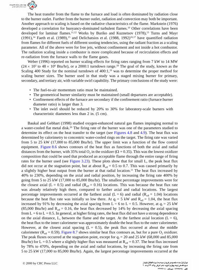
The heat transfer from the flame to the furnace and load is often dominated by radiation closeto the burner outlet. Further from the burner outlet, radiation and convection may both be important.Another approach to scaling is based on the radiative characteristics of the flame. Markstein (1976)developed a correlation for buoyancy-dominated turbulent flames.10 Other correlations have beendeveloped for laminar flames.11,12 Works by Buriko and Kuznetsov (1978),13 Turns and Mayr(1991),14 Faeth et al. (1989),15 and Delichatsios et al. (1988, 1992)16,17 have quantified radiationfrom flames for different fuels of different sooting tendencies, using the radiant fraction as a scalingparameter. All of the above were for free jets, without confinement and not inside a hot combustor.The radiation scaling inside a combustor is more complicated because of recirculation effects andre-radiation from the furnace walls to the flame gases.
Weber (1996) reported on burner scaling effects for firing rates ranging from 7 kW to 14 MW(24 × 103 to 48 × 106 Btu/hr), or a 2000:1 turndown range.18 The goal of the study, known as theScaling 400 Study for the nominal turndown of 400:1,19 was to determine the proper method forscaling burner sizes. The burner used in that study was a staged mixing burner for primary,secondary, and tertiary air, with variable swirl capability. The primary conclusions of the study were:
• The fuel-to-air momentum ratio must be maintained.• The geometrical burner similarity must be maintained (small departures are acceptable).• Confinement effects of the furnace are secondary if the confinement ratio (furnace:burner
diameter ratio) is larger than 3.• The inlet swirl should be reduced by 20% to 30% for laboratory-scale burners with
characteristic diameters less than 2 in. (5 cm).
Baukal and Gebhart (1998) studied oxygen-enhanced natural gas flames impinging normal toa water-cooled flat metal disk.20 The firing rate of the burner was one of the parameters studied todetermine its effect on the heat transfer to the target (see Figures 4.8 and 4.9). The heat flux wasdetermined by calorimetry to concentric water-cooled rings on the target. The firing rate was variedfrom 5 to 25 kW (17,000 to 85,000 Btu/hr). The upper limit was a function of the flow controlequipment. Figure 8.6 shows contours of the heat flux as functions of both the axial and radialdistances from the burner, with 35% total O2 in the oxidizer (Ω = 0.35). This was the lowest oxidizercomposition that could be used that produced an acceptable flame through the entire range of firingrates for the burner used (see Figure 3.23). These plots show that for small L, the peak heat fluxdid not occur at the stagnation point, but at about Reff = 0.5 to 0.7. This was caused primarily bya slightly higher heat output from the burner at that radial location.21 The heat flux increased by40% to 230%, depending on the axial and radial position, by increasing the firing rate 400% bygoing from 5 to 25 kW (17,000 to 85,000 Btu/hr). The smallest percentage improvements were forthe closest axial (L = 0.5) and radial (Reff = 0.16) locations. This was because the heat flux ratewas already relatively high there, compared to farther axial and radial locations. The largestpercentage improvements occurred at the farthest axial (L = 6) and radial (Reff = 1.04) locationsbecause the heat flux rate was initially so low there. At qf = 5 kW and Reff = 1.04, the heat fluxincreased by 91% by decreasing the axial spacing from L = 6 to L = 0.5. However, at qf = 25 kW(85,000 Btu/hr) and Reff = 0.16, the heat flux decreased by 14% by decreasing the axial spacingfrom L = 6 to L = 0.5. In general, at higher firing rates, the heat flux did not have a strong dependenceon the axial distance, L, between the flame and the target. At the farthest axial location (L = 6),the heat flux to the inner calorimeter was approximately double the heat flux to the outer calorimeter.However, at the closest axial spacing (L = 0.5), the peak flux occurred at about the middlecalorimeter (Reff = 0.59). Figure 8.7 shows similar heat flux contours as, but for a pure O2 oxidizer.The peak fluxes occurred at the stagnation point, except for qf = 20 and 25 kW (68,000 and 85,000Btu/hr) for L = 0.5 where a slightly higher flux was measured at Reff = 0.37. The heat flux increasedby 78% to 470%, depending on the axial and radial locations, by increasing the firing rate from5 to 25 kW (17,000 to 85,000 Btu/hr). Again, the largest percentage improvements occurred at the
© 2000 by CRC Press LLC

farthest locations, while the smallest improvements occurred at the closest locations. Unlike theΩ = 0.35 data in, the heat flux strictly increased, by 42% to 230%, as the axial spacing decreasedfor the Ω = 1.00 data in Figure 8.7. Like the Ω = 0.35 data, at large axial spacings, the heat fluxto the innermost calorimeter was approximately double the flux to the outermost calorimeter.Figure 8.8 shows how the heat flux to the innermost calorimeter was affected by the axial locationof the target and by the burner firing rate. The heat flux increased with the firing rate and decreasedwith the axial distance. The shape of the contour lines was significantly different for the Ω = 0.35flames, compared to the Ω = 1.00 flames. The peak flux occurred at an intermediate axial location(ÝL = 2) for the Ω = 0.35 flames. For the Ω = 1.00 flames, the heat flux strictly increased as theaxial spacing decreased. Figure 8.9 shows that for Ω = 1.00 and large L, the heat flux increasedrapidly with the firing rate. The shape of each curve is similar. In all cases, the heat flux increasedwith the firing rate and decreased with the axial spacing. The thermal efficiency, η, was defined as:
(8.8)
FIGURE 8.6 Contours of the total heat flux, q″ (kW/m2), from stoichiometric natural gas flames (Ω = 0.35)with various firing rates (qf = 5 to 25 kW) impinging on the surface of an untreated stainless target. (FromC.E. Baukal and B. Gebhart, Exp. Therm. Fluid Sci., 16(3), 247-259, 1998.)
η =
′′=
∑q A
q
i i
i 1
5
f
© 2000 by CRC Press LLC

where q″i was the calculated heat flux to ring i, Ai was the impingement surface area of ring i, andqf was the burner firing rate. The efficiency was then the total energy absorbed by the first fivecalorimeters, divided by the burner firing rate. Figure 8.10 shows how the thermal efficiency variedwith the firing rate, oxidizer composition, and axial location. The efficiency decreased with L,increased with Ω, and decreased with the firing rate. At Ω = 1.00 and qf = 5 kW (17,000 Btu/hr),the efficiency decreased rapidly from L = 4 to L = 6 because, at L = 6, the visible flame lengthwas less than the distance between the burner and the target. Buoyancy effects were visually evident,as the flame shape was highly transient and wavy. Air infiltration may have significantly reducedthe heat flux to the target for that set of conditions.
8.2.4 FLAME SHAPE EFFECTS
Hutchinson et al. (1975) experimentally and numerically showed that a quarl (burner block or tile)shortened the flame on an air/natural gas burner with swirl firing into a water-cooled cylindricalfurnace.21a The recirculation zone in the furnace was pulled closer to the burner with the quarl,compared to the same burner without a quarl. Higher temperatures and heat fluxes were measured
FIGURE 8.7 Contours of the total heat flux, q″ (kW/m2), from stoichiometric natural gas flames (Ω = 1.00)with various firing rates (qf = 5 to 25 kW) impinging on the surface of an untreated stainless target. (FromC.E. Baukal and B. Gebhart, Exp. Therm. Fluid Sci., 16(3), 247-259, 1998.)
© 2000 by CRC Press LLC

closer to the burner with the quarl, than without the quarl. The quarl shortened the flame and movedthe heat release closer to the burner. The calculations showed that the convective heat transfer andthe radiative heat transfer to the furnace wall were of the same order with or without the quarl.
One recent burner development trend in about the last decade has been the development of so-called flat-flame burners. This can mean different things, but here it refers to a rectangular flameshape, as opposed to the traditional round flame shape. The goal is to have a higher flame surfacearea to increase the area that radiates from the flame to the load. This trend in burner design hasbeen particularly evident in the use of oxygen-enriched burners in the glass and aluminum industries.If the trend continues, this type of flame will likely be applied to other industrial heating andmelting applications.
There are numerous examples of the use of flat flames in glass melting. Kirilenko et al. (1988)described a flat-flame burner used in a regenerative glass-melting furnace.22 Ibbotson (1991)described a technique for lancing a fan-shaped jet of oxygen under a fuel port in a glass-meltingfurnace to improve temperature uniformity and minimize hotspots.23
Flat shaped flames have also been used in aluminum melting. Yap and Pourkashanian (1996)reported on a flat-flame oxy/fuel burner, which they described as a large aspect-ratio flame.24 Theburner was claimed to have more uniform heat transfer rates, compared to conventional round flame
FIGURE 8.8 Contours of the total heat flux, q″ (kW/m2), from stoichiometric natural gas flames of variousfiring rates (qf = 5 to 25 kW) and oxidizer compositions (Ω = 0.35 and 1.00) to the stagnation point (Reff = 0.16)of an untreated brass target. (From C.E. Baukal and B. Gebhart, Exp. Therm. Fluid Sci., 16(3), 247-259, 1998.)
© 2000 by CRC Press LLC

burners. The burner also had excellent flame stability, resulting in a wide operating range, low NOxemissions, and high flame luminosity. The combination of low NOx emissions and high luminosity,both of which are important in most heating applications, is a unique aspect of the burner. Inaddition, the burner minimized oxidation of the molten aluminum, which maximizes the productyield.
The length of the flame influences the heat transfer as longer flames may be more luminousat lower temperature compared to similar flames at the same operating conditions. Blake andMcDonald (1993) have correlated visible flame length data for vertical turbulent diffusion flamesas follows:25
(8.9)
where lf is the flame length, df is the flame diameter, J is the momentum of the source jet, ρ× isthe density of the ambient, g is the gravitational constant, and α1 and α2 are constants as given inTable 8.1. The fraction inside the parentheses in Equation 8.9 is referred to as the density weightedFroude number.
Figure 8.11 shows how the visible flame length for an open-flame diffusion burner varies as afunction of the firing rate and oxidizer composition.26 The flame length was nearly the same forlower firing rates. At higher firing rates, the pure O2 flames (Ω = 1.00) were longer than the lowerpurity flames (Ω = 0.35). The flame length affects the flame shape, which influences the radiatingarea of the flame.
FIGURE 8.9 Total heat flux (q″) from stoichiometric natural gas flames (Ω = 1.00) of various firing rates(qf) impinging on the stagnation point (Reff = 0.16) of an untreated stainless target. (From C.E. Baukal and B.Gebhart, Exp. Therm. Fluid Sci., 16(3), 247-259, 1998.)
l
dJgd
f
f f
=π
⎛
⎝⎜
⎞
⎠⎟
∞
αρ
α
1 3
42
© 2000 by CRC Press LLC
FIGURE 8.10 Thermal efficiency (η) for stoichiometric natural gas flames of various firing rates (qf = 5 to 25kW) and oxidizer compositions (Ω = 0.35 and 1.00). (From C.E. Baukal and B. Gebhart, Exp. Therm. Fluid Sci.,16(3), 247-259, 1998.)
TABLE 8.1Constants for Flame Length Equation
4J/¼ρ×gd 3f α1 α2
10–9–10–6 6.73 0.20910–6–10–4 7.79 0.21810–4–10–1 7.25 0.184
Source: Adapted from T.R. Blakeand M. McDonald, Comb. Flame,
94, 426-432, 1993.
© 2000 by CRC Press LLC

8.3 RADIANT BURNERS
Radiant burners operate by combusting a fossil fuel, which heats a solid surface that radiates infrared(IR) energy to a load. These burners are used in a number of lower temperature heating and dryingapplications including, for example:
• Drying paper and cardboard in a paper mill• Paper finishing• Drying wood• Porcelain frit drying• Curing ceiling tiles• Teflon curing• Drying and curing coatings on paper and metals• Curing ink on paper and powder coat paints• Baking in mass food preparation• Setting dyes in textile and carpet production, sometimes referred to as pre-drying• Curing lens assemblies in automotive headlamp assembly manufacturing• Plastics curing
Both gas-fired and electric radiant heaters are commonly used; however, gas-fired radiant burnershave lower operating costs due to the difference between the cost of electricity and natural gas inmost locations. Pettersson and Stenström (1998) compared gas-fired and electric IR heaters in twopaper-coating drying processes.27 The efficiencies of the gas-fired and electric dryers were 30%and 40%, respectively. However, there was considerable uncertainty in the measurements due tothe difficulty in obtaining accurate moisture measurements of the paper being dried. Even if theefficiencies are correct, the gas-fired system may still be more economical, depending on the costof electricity vs. natural gas.
FIGURE 8.11 Flame length as function of firing rate and oxidizer composition for stoichiometric naturalgas flames. (From C.E. Baukal and B. Gebhart, Int. J. Heat Mass Transfer, 44(11), 2539-2547, 1997.)
© 2000 by CRC Press LLC

Radiant burners are designed to produce a uniform surface temperature heat source for heatingand melting a variety of materials (see Chapter 10). The uniform surface temperature producesmore homogeneous heating of the materials, which normally improves the product quality comparedto conventional burners that may produce hotspots. Other advantages of these burners may include:
• High thermal efficiencies• Low pollutant emissions• Directional heating• Very fast response time to load changes• Very fast heating compared to convective heating• Burner shape can be tailored to the shape of the heat load to optimize heat transfer• Ability to segment a burner to produce a nonuniform heat output profile, which may be
useful in certain types of heating and drying applications• Certain types of radiant burners have very rapid heat-up and cool-down times• No open flames that could ignite certain types of materials (e.g., paper or textiles)• More control over the heating process because of the known and measurable surface
temperature of the radiant surfaces compared to open flames, where the flame temper-ature is very difficult to measure
• Burners are very modular and can be configured in a wide variety of geometries toaccommodate the process heating requirements
The primary parameters of interest for radiant burners are the power density (firing rate perunit area), radiant efficiency (fraction of fuel heating value converted to thermal radiation), heat-up and cool-down times, and pollutant emissions. Other factors of importance include cost, dura-bility, and longevity.
There are also some important limitations of porous refractory burners, compared to moreconventional open-flame burners, which may include:
• Relatively low temperature limit for the radiant surface due to the limits of the refractorymaterial
• Fuel and oxidizer must be clean to avoid plugging the porous radiant surface, whichessentially precludes the use of fuels like coal or heavy fuel oil
• Some of the radiant surfaces can be damaged by water or by contact with solid materials,which may be prevalent in certain applications
• Holes in the radiant surface can cause flashback since these burners use premix• Some designs may have high pressure drops, which means more energy is needed for
the blower to flow the combustion air through the ceramic burner material• Due to the limits in radiant surface temperatures, the firing rate density is usually limited• Some types of radiant burners using hard ceramic surfaces may have high heat capaci-
tances that could ignite certain load materials upon a sudden line stoppage
In these burners, fuel and air are premixed and combusted either just inside a radiating surfaceor just above the surface, depending on the operating conditions and specific radiant burner design.If the mixture velocity is too low, flashback or flame extinguishment may occur, depending on thedesign of the burner. Besides the operational considerations, flashback is an obvious safety concern.If the mixture velocity is too high, the flame may blow off or the radiant performance may beseverely reduced because the burner surface is not being directly heated by the hot exhaust products.Depending on the specific design of the burner, optimum performance is achieved when the flameis stabilized just inside or just above the outer burner outlet.
Howell et al. (1995) referred to the burner material as “porous inert media” and presented areview of these types of burners, which have been made from a wide variety of ceramics that often
© 2000 by CRC Press LLC

include alumina, zirconia, or silicon carbide.28 Hsu and Howell (1993) developed the followingequation for the effective thermal conductivity of partially stabilized zirconia (PSZ) (zirconiumoxide plus <3% magnesium oxide) for temperatures in the range of 290K to 890K (63°F to 1140°F)and for sample pore sizes from 10 to 65 pores per inch (ppi):29
k (W/m-K) = 0.188 – 0.0175 d (8.10)
where d is the actual pore size of the material in (in millimeters) and 0.3 < d < 1.5 mm.Speyer et al. (1997) studied the performance of four different types of commercial gas-fired
radiant burners: a metal (Fe-Cr-Al) fiber (~40 µm diameter) burner, a reticulated ceramic burnermade of a porous cordierite (Mg2Al4Si5O18), a porous single unit mullite (Al6Si2O13) tile burner,and a flame impingement burner where the products of combustion are forced around a metalscreen that radiates to the load.30 The study was sponsored by the Gas Research Institute (Chicago,IL). The thermal efficiencies as a function of the combustion intensity are shown in Table 8.2. Theefficiency was determined by measuring the radiant output or radiosity from the burner surface andwas calculated using:
(8.11)
where e is the calculated efficiency, RT is the measured radiosity, •
Vg is the volume flow rate of thefuel, Hc is the heating value of the fuel, and A is the surface area of the burner. The experimentalresults showed that the peak radiosity measurements as a function of the air-to-fuel mixture ratiooccurred for percent excess fuels ranging from 6% to 7.5%, depending on the specific burner design.Similar results were calculated for the radiant efficiencies. Preheating the air/fuel mixture increasedboth the radiosity and thermal efficiencies, essentially in a linear manner for mixture temperaturesranging from 40°C to 155°C (100°F to 311°F). In most cases, the efficiency declined with com-bustion intensity, except for the reticulated ceramic and metal fiber with perforations and a frontmetal screen, both of which had peak efficiencies at intermediate combustion intensities. The flameimpingement and ported ceramic burners were the most efficient, while the metal fiber with andwithout perforations was the least efficient. The study also showed that the thermal efficiencygenerally increased as the fraction of closed area increased on the burner surface.
The heat transfer coefficient between the hot exhaust products and the radiant burner materialis difficult to predict and measure due to the uncertainty in the surface area of the ceramic structure.These coefficients have traditionally been presented in terms of a volumetric coefficient (Btu/hr-°F-ft3 or kW/°C-m3). Chen et al. (1987) assumed the coefficient was large enough that the temperature
TABLE 8.2Comparison of Thermal Efficiencies for Radiant Burners
Radiant Burner TypeCombustion Intensity
(kW/m2)Thermal Efficiency Range
(%)
Metal fiberNo perforations 150–540 18–26With perforations 150–540 16–27With perforations & front metal screen 100–440 22–38
Reticulated ceramic 150–630 27–39Ported ceramic 140–520 37–54Flame impingement 150–430 46–52
Source: Adapted from R.F. Speyer, W.-Y. Lin, and G. Agarwal, Exp. Heat Transfer, 9, 213-245, 1996.
eR
V H AT
g c
= ˙ ∆
© 2000 by CRC Press LLC

of the solid was essentially the same as the temperature of the hot flowing gas.31 Sathe et al. (1990)used a value of 2 × 10⁹ W/m3-K (1 × 10⁸ Btu/hr-°F-ft3) computed for cylinders in crossflow.32 Hsuet al. (1993) used 107 W/m3-K (5 × 10⁵ Btu/hr-°F-ft3).33 Younis and Viskanta (1993) empiricallydetermined the following correlation for alumina and cordierite ceramic foams with pore diametersranging from 0.29 to 1.52 mm (0.011 to 0.0598 in.):34
(8.12)
where d is the actual pore diameter and L is the thickness of the specimen in the flow direction.Fu et al. (1998) noted the relationship between the volumetric heat transfer coefficient hv and theconvection coefficient h:35
hv = av h (8.13)
where av can be computed using the following empirical equation:
av = 169.4 PPC (m2/m3) (8.14)
where PPC is the number of pores per centimeter for cellular ceramics. Four different choices forthe characteristic dimension were identified:
the reciprocal of the surface area: da = 1/av (8.15)
the hydraulic diameter: dh = 4φ/av (8.16)
the mean pore diameter: (8.17)
and
the ratio of the inertial to the viscous friction coefficients: dr = β/α (8.18)
where φ is the porosity, β is the inertia coefficient in the Reynolds-Forchheimer equation, and αis the viscous coefficient in the Reynolds-Forchheimer equation. The following empirical correla-tions, using each of these characteristic dimensions, were developed for specimens having a PPCranging from 4 to 26:
(8.19)
(8.20)
(8.21)
(8.22)
Nu = − ( )[ ] + ( )[ ]0 819 1 7 33 0 36 1 15. . Re .d L
d L
dm =π ( )4φ
PPCcm
Nu for vm
d dL d m m= +
⎡
⎣⎢
⎤
⎦⎥ ≤ ≤0 0426
1 2362 836.
.Re Re
Nu for vh
d dL d h h= +
⎡
⎣⎢
⎤
⎦⎥ ≤ ≤0 0730
1 3023 1594.
.Re Re
Nu for va
d dL d a a= +
⎡
⎣⎢
⎤
⎦⎥ ≤ ≤0 0252
1 2801 480.
.Re Re
Nu for 0. 2vr
d dL d r r= +
⎡
⎣⎢
⎤
⎦⎥ ≤ ≤0 000267
1 4470 2 4.
.Re Re .
© 2000 by CRC Press LLC

where Nuv is the volumetric Nusselt number, defined as:
(8.23)
where lc is the characteristic pore length and k is the thermal conductivity of the gas. The uncertaintyin the correlations was largest for the smaller Reynolds numbers.
One of the challenges of gas-fired infrared burners is determining the radiant efficiencies. Mitalet al. (1998) noted a wide discrepancy in the reported radiant efficiencies (varying by more than200%) for radiant burners.36 Part of the discrepancy was attributed to a lack of a standard measure-ment technique to determining the efficiency. Other problems include nondiffuse radiation fromthe burners and nonuniform burner surfaces. They presented a technique that is not sensitive toburner surface nonuniformities. Typical results for a reticulated ceramic foam radiant burner areshown in Figure 8.12. A calorimetric method was used to check the consistency of the data. It wasshown that single-point radiation measurements can deviate considerably from more rigorous multi-point measurement techniques. Yetman (1993) described a simple technique for measuring the totalradiant output of an infrared burner using a narrow angle pyrometer.37 Johansson (1993) presenteda method for measuring the spectral output of radiant burners using an infrared spectrometer.38
Madsen et al. (1996) measured the spectral radiation from several types of radiant burners asshown in Figure 8.13.39 As can be seen, the spectra are fairly similar that have distinctive peaksaround 3 and 4.5 µm. This shows the selective emittance of certain types of radiant burners andthe possibility of matching the burner to the load spectral absorptivity to optimize heat transferefficiency.
8.3.1 PERFORATED CERAMIC OR WIRE MESH RADIANT BURNERS
Examples of these types of burners are shown in Figure 8.14. Perforated or ported ceramic burnersmay consist of a pressed ceramic plate, which may include prepunched holes, where the flamesheat the surface directly.40 The surface can be textured to further enhance the radiant efficiency ofthe burner. New developments in ceramic foams are being applied to this type of burner. Thesefoams are often less expensive to make than perforated ceramics. They provide a higher surfacearea for radiation and a more uniform heating surface, compared to perforated ceramics. Manyshapes are possible with the ceramic foams and the pore size is adjustable. Flanagan et al. (1992)described the use of a ported ceramic burner, shown in Figure 8.15, to achieve low NOx emissions.41
However, the burner was actually fired at up to 15 times its normal maximum design firing rate sothat the flames were highly lifted and therefore did not radiate from the surface as in normaloperation. Mital and Gore (1994) discussed the use of a reticulated ceramic insert to enhanceradiation heat transfer in direct-fired furnaces.42 The insert was placed downstream of the outlet ofa laminar diffusion flame, as shown in Figure 8.16. Experimental results showed up to a 60%improvement in radiative heat flux compared to the case with no insert. The radiative heat fluxwith and without the insert is shown in Figure 8.17. Kataoka (1998) described a new type of high-temperature porous ceramic burner made of aluminum titanate (Al2TiO5), capable of surfacetemperatures up to 1100°C (2000°F).43
Wire mesh burners are made from high-temperature resistant metals, such as stainless steelsor inconel. The open area in the mesh serves as the port area for the burner. However, due to thehigh thermal conductivity of metals, several layers of mesh are often required to prevent flashback.The thermal conductivity between the layers is much less than through the mesh itself because ofthe contact resistance between the layers. An important problem with wire mesh radiant burnersare the lower temperature limits compared to ceramic burners, due to the temperature limits of themetals.
Nuvv ch l
k=
2
© 2000 by CRC Press LLC
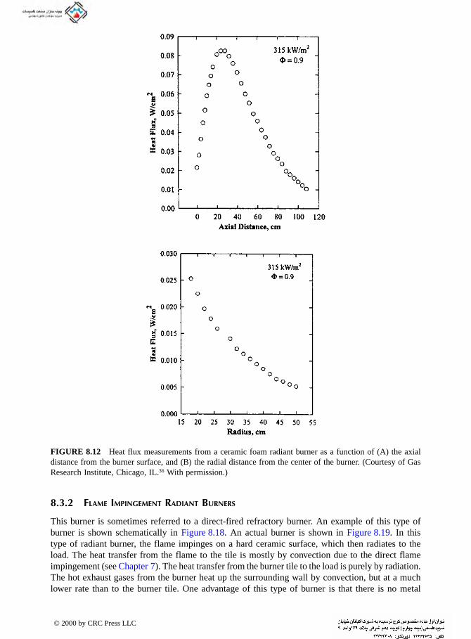
8.3.2 FLAME IMPINGEMENT RADIANT BURNERS
This burner is sometimes referred to a direct-fired refractory burner. An example of this type ofburner is shown schematically in Figure 8.18. An actual burner is shown in Figure 8.19. In thistype of radiant burner, the flame impinges on a hard ceramic surface, which then radiates to theload. The heat transfer from the flame to the tile is mostly by convection due to the direct flameimpingement (see Chapter 7). The heat transfer from the burner tile to the load is purely by radiation.The hot exhaust gases from the burner heat up the surrounding wall by convection, but at a muchlower rate than to the burner tile. One advantage of this type of burner is that there is no metal
FIGURE 8.12 Heat flux measurements from a ceramic foam radiant burner as a function of (A) the axialdistance from the burner surface, and (B) the radial distance from the center of the burner. (Courtesy of GasResearch Institute, Chicago, IL.36 With permission.)
© 2000 by CRC Press LLC
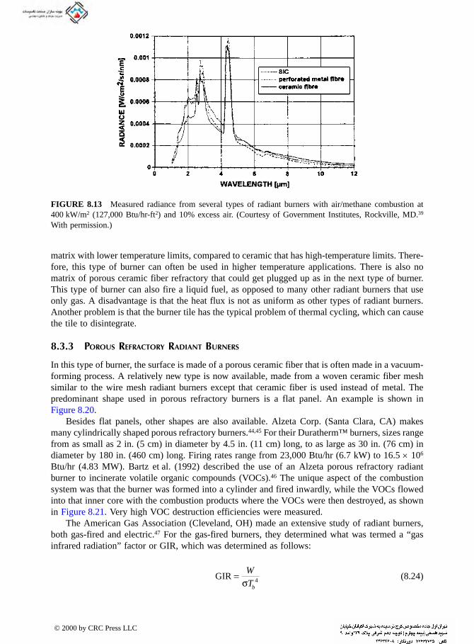
matrix with lower temperature limits, compared to ceramic that has high-temperature limits. There-fore, this type of burner can often be used in higher temperature applications. There is also nomatrix of porous ceramic fiber refractory that could get plugged up as in the next type of burner.This type of burner can also fire a liquid fuel, as opposed to many other radiant burners that useonly gas. A disadvantage is that the heat flux is not as uniform as other types of radiant burners.Another problem is that the burner tile has the typical problem of thermal cycling, which can causethe tile to disintegrate.
8.3.3 POROUS REFRACTORY RADIANT BURNERS
In this type of burner, the surface is made of a porous ceramic fiber that is often made in a vacuum-forming process. A relatively new type is now available, made from a woven ceramic fiber meshsimilar to the wire mesh radiant burners except that ceramic fiber is used instead of metal. Thepredominant shape used in porous refractory burners is a flat panel. An example is shown inFigure 8.20.
Besides flat panels, other shapes are also available. Alzeta Corp. (Santa Clara, CA) makesmany cylindrically shaped porous refractory burners.44,45 For their Duratherm™ burners, sizes rangefrom as small as 2 in. (5 cm) in diameter by 4.5 in. (11 cm) long, to as large as 30 in. (76 cm) indiameter by 180 in. (460 cm) long. Firing rates range from 23,000 Btu/hr (6.7 kW) to 16.5 × 10⁶
Btu/hr (4.83 MW). Bartz et al. (1992) described the use of an Alzeta porous refractory radiantburner to incinerate volatile organic compounds (VOCs).46 The unique aspect of the combustionsystem was that the burner was formed into a cylinder and fired inwardly, while the VOCs flowedinto that inner core with the combustion products where the VOCs were then destroyed, as shownin Figure 8.21. Very high VOC destruction efficiencies were measured.
The American Gas Association (Cleveland, OH) made an extensive study of radiant burners,both gas-fired and electric.47 For the gas-fired burners, they determined what was termed a “gasinfrared radiation” factor or GIR, which was determined as follows:
(8.24)
FIGURE 8.13 Measured radiance from several types of radiant burners with air/methane combustion at400 kW/m2 (127,000 Btu/hr-ft2) and 10% excess air. (Courtesy of Government Institutes, Rockville, MD.39
With permission.)
GIR = WTbσ 4
© 2000 by CRC Press LLC

where W = Q/A is the total normal infrared radiation from the burner measured by a spectropho-tometer, σ is the Stefan-Boltzman constant, and Tb is the absolute brightness temperature of theburner surface measured with an optical pyrometer. The GIR factor was similar to a burneremissivity. However, for some of the burners, the GIR factor exceeded 1.0. The GIR factor wasapproximately 15% higher than the true burner surface emissivity. This is due to the gaseousnonluminous radiation in addition to the surface radiation from the burner. For the burners tested,the GIR factor ranged from 0.36 to 1.17, depending on the burner type.
FIGURE 8.14 Examples of porous ceramic and wire mesh radiant burners. (From F. Ahmady, ProcessHeating, 1(2), 38-43, 1994. Courtesy of Solaronics, Rochester, MI. With permission.)
© 2000 by CRC Press LLC
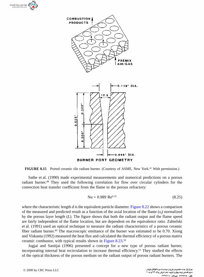
Sathe et al. (1990) made experimental measurements and numerical predictions on a porousradiant burner.48 They used the following correlation for flow over circular cylinders for theconvection heat transfer coefficient from the flame to the porous refractory:
Nu = 0.989 Re0.33 (8.25)
where the characteristic length d is the equivalent particle diameter. Figure 8.22 shows a comparisonof the measured and predicted result as a function of the axial location of the flame (xf) normalizedby the porous layer length (L). The figure shows that both the radiant output and the flame speedare fairly independent of the flame location, but are dependent on the equivalence ratio. Zabielskiet al. (1991) used an optical technique to measure the radiant characteristics of a porous ceramicfiber radiant burner.49 The macroscopic emittance of the burner was estimated to be 0.70. Xiongand Viskanta (1992) measured the heat flux and calculated the thermal efficiency of a porous matrixceramic combustor, with typical results shown in Figure 8.23.50
Jugjai and Sanitjai (1996) presented a concept for a new type of porous radiant burner,incorporating internal heat recirculation to increase thermal efficiency.51 They studied the effectsof the optical thickness of the porous medium on the radiant output of porous radiant burners. The
FIGURE 8.15 Ported ceramic tile radiant burner. (Courtesy of ASME, New York.41 With permission.)
© 2000 by CRC Press LLC

FIGURE 8.16 Laminar flame with and without a ceramic insert. (Courtesy of ASME, New York.42 Withpermission.)
FIGURE 8.17 Radiant heat flux as a function of axial position for a laminar flame (A) with and (B) withouta ceramic insert. (Courtesy of ASME, New York.42 With permission.)
© 2000 by CRC Press LLC

optical thickness was increased by added layers of stainless steel wire mesh that formed the porousmedium for the burners tested. The added layers improved the heat transfer from the hot gases tothe porous medium.
Mital et al. (1996) claimed to have made the first measurements of temperature and speciesdistributions inside submerged flames stabilized inside porous ceramic burners.52 They noted the widediscrepancy in the performance of these burners in the literature and in manufacturers’ litererature.
Rumminger et al. (1996) developed a one-dimensional model of a bilayered reticulated ceramicsradiant burner.53 The model results showed that for a “submerged flame” where the flame is anchoredinside the porous refractory, nearly all of the important reactions occur inside the porous medium.This complicates the study for this type of burner because of the difficulty in making measurementsinside the porous medium. They speculate that it is possible the large internal surface area of theporous medium could affect the chemistry, but there is no data at this time to confirm that possibility.
Van der Drift et al. (1997) studied various coatings on porous foam ceramic infrared burnersto determine the effects on heat transfer to wet paper and to three colors (white, blue, and black).54
They showed that there can be up to a 10% improvement using coated burners compared to a base-case metal fiber burner.
FIGURE 8.18 Schematic of a flame impingement radiant burner. (Courtesy of American Gas Association,Cleveland, OH.47 With permission.)
FIGURE 8.19 InfraRad ceramic radiant infrared burner. (Courtesy of Eclipse, Rockford, IL.)
© 2000 by CRC Press LLC

Mital et al. (1998) made experimental measurements on a bilayered reticulated ceramic foammade of Cordierite.55 Measurements included radiation efficiency using a heat flux gage and burnersurface measurements with a type R thermocouple. Radiation efficiency results are shown inFigure 8.24, which include both single and multi-point measurements and model predictions.
8.3.4 ADVANCED CERAMIC RADIANT BURNERS
Tong et al. (1989) showed through computer modeling that the performance of porous radiantburners can be improved by as much as 109% using submicron diameter ceramic fibers.56 Bellet al. (1992) described a staged porous ceramic burner that demonstrated low NOx emissions.57
Kendall and Sullivan (1993) studied enhancing the radiant performance of porous surface radiantburners using improved ceramic, high-temperature, high-emissivity fibers.58 Selective emissivity
FIGURE 8.20 Flat-panel infrared burner. (Courtesy of Marsden, Inc., Pennsauken, NJ.)
FIGURE 8.21 Inwardly fired porous refractory radiant burner, with heat recovery, for VOC destruction.(Courtesy of ASME, New York.46 With permission.)
© 2000 by CRC Press LLC

was achieved by coating a standard ceramic fiber burner with an outer layer of ytterbia. The outputof the uncoated vs. the coated burner is shown in Figure 8.25. As can be seen, there is a large spikein the output of the coated burner at around 1 µm. However, there was not a significant improvementin performance and the durability was in question. In certain applications, there may be a need tohave a burner with selective radiant emissions corresponding to selective absorption in the load.Potential applications include glass melting, glass bending and lamination, thin-film drying, andindirect heating. Xiong et al. (1993) described a porous ceramic surface combustor-heater with abuilt-in heat exchanger for improving the thermal efficiency, as shown in Figure 8.26.59 Ruiz andSingh (1993) described an advanced infrared burner shown in Figure 8.27.60 Figure 8.28 shows thatthe new burner design has considerably higher radiant outputs than the previous style design. Thenew burner increased a powder paint drying process by 40% and a paper drying process by 200%.Severens et al. (1995) modeled porous radiant burners.61 The 1-D model results compared favorablywith experimental data for the radiant fraction as a function of the gas velocity through the burner.
FIGURE 8.22 Measured and predicted flame speed and radiant output for a porous radiant burner. (Courtesyof The Combustion Institute, Pittsburgh, PA.48 With permission.)
FIGURE 8.23 Average heat transfer rate and thermal efficiency as a function of firing rate for a porousceramic matrix burners. (Courtesy of ASME, New York.50 With permission.)
© 2000 by CRC Press LLC

FIGURE 8.24 Predicted and measured radiation efficiency for a porous radiant burner at an equivalenceratio of 0.9. (Courtesy of The Combustion Institute. Pittsburgh, PA.55 With permission.)
FIGURE 8.25 Emission spectra of a ytterbia fiber burner compared to an Alzeta (Santa Clara, CA) Pyrocoreburner, both operating at 127,000 Btu/hr-ft2 (400 kW/m2). (Courtesy of GRI Gas Research Institute, Chicago,IL.58 With permission.)
© 2000 by CRC Press LLC

Bogstra (1998) described a new type of infrared radiant burner, referred to as CHERUB, with aclosed surface to separate the combustion exhaust gases from the product being heated.62 The burnerhad an enclosed, flat, multi-burner system that heated a ceramic radiant plate. The burner wasreported to have a radiant efficiency of 80%, compared to an efficiency of 40% for conventionalhigh-temperature radiant burners.
As previously discussed, one of the limitations of porous refractory burners is the burner surfacetemperature. If the firing rate density is to be increased, new refractory materials are needed that
FIGURE 8.26 Surface combustor-heater concept. (Courtesy of Government Institutes, Rockville, MD.59
With permission.)
FIGURE 8.27 Advanced infrared burner. (Courtesy of Government Institutes, Rockville, MD.60 With per-mission.)
© 2000 by CRC Press LLC
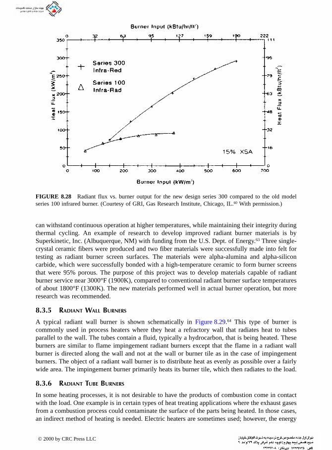
can withstand continuous operation at higher temperatures, while maintaining their integrity duringthermal cycling. An example of research to develop improved radiant burner materials is bySuperkinetic, Inc. (Albuquerque, NM) with funding from the U.S. Dept. of Energy.63 Three single-crystal ceramic fibers were produced and two fiber materials were successfully made into felt fortesting as radiant burner screen surfaces. The materials were alpha-alumina and alpha-siliconcarbide, which were successfully bonded with a high-temperature ceramic to form burner screensthat were 95% porous. The purpose of this project was to develop materials capable of radiantburner service near 3000°F (1900K), compared to conventional radiant burner surface temperaturesof about 1800°F (1300K). The new materials performed well in actual burner operation, but moreresearch was recommended.
8.3.5 RADIANT WALL BURNERS
A typical radiant wall burner is shown schematically in Figure 8.29.64 This type of burner iscommonly used in process heaters where they heat a refractory wall that radiates heat to tubesparallel to the wall. The tubes contain a fluid, typically a hydrocarbon, that is being heated. Theseburners are similar to flame impingement radiant burners except that the flame in a radiant wallburner is directed along the wall and not at the wall or burner tile as in the case of impingementburners. The object of a radiant wall burner is to distribute heat as evenly as possible over a fairlywide area. The impingement burner primarily heats its burner tile, which then radiates to the load.
8.3.6 RADIANT TUBE BURNERS
In some heating processes, it is not desirable to have the products of combustion come in contactwith the load. One example is in certain types of heat treating applications where the exhaust gasesfrom a combustion process could contaminate the surface of the parts being heated. In those cases,an indirect method of heating is needed. Electric heaters are sometimes used; however, the energy
FIGURE 8.28 Radiant flux vs. burner output for the new design series 300 compared to the old modelseries 100 infrared burner. (Courtesy of GRI, Gas Research Institute, Chicago, IL.60 With permission.)
© 2000 by CRC Press LLC

costs are considerably higher than the cost of fossil-fuel-fired heaters. The burner of choice forindirect heating is typically a radiant tube.
The objective of the radiant tube burner is to efficiently transfer heat from the combustion gasesto the radiant tube, and then to efficiently radiate that energy to the load. There are several challengesthat need to be considered when using radiant tubes. The biggest challenge is the material ofconstruction for the tube itself. Typical tubes are constructed of high-temperature metal alloys orof ceramics. Metal alloys can be expensive and typically do not have as high a continuous operatingtemperature as ceramics. Metal tube burners typically operate at temperatures around 2000°F(1400K). These tubes can fail, due to a variety of metallurgical problems related to the high-temperature operation and thermal cycling of the burners. Metal tubes are more commonly usedthan ceramic tubes, and research continues into higher temperature metals for use in metallic radianttube burners.65,66 Ceramic tubes tend to have higher temperature operating limits compared to themetal tubes, but are even more susceptible to thermal shock. Research also continues on newceramic materials for radiant tube burners.66a,67,68 There may also be problems joining the ceramictubes to the metal burner body due to the differences in thermal expansion that can cause theceramic tubes to crack. The Institute of Gas Technology (Chicago, IL) is working on a newcomposite material for radiant tubes that is silicon carbide based and has a working temperatureexceeding 2450°F (1620K).69 These new tubes have excellent shock resistance and are capable ofheat flux rates up to 150 Btu/hr-in.2 (68 kW/m2), compared to rates of 55 Btu/hr-in.2 (25 kW/m2)for metallic radiant tubes. Tube lives may be increased by as much as 3 times with the new tubes.The Gas Research Institute (1998) has funded many projects related to the use of advanced ceramiccomposite materials for radiant tube burners.70 GRI estimated that about 40% of the more than
FIGURE 8.29 Typical radiant wall burner. (Courtesy of American Petroleum Institute, Washington, D.C.64
With permission.)
© 2000 by CRC Press LLC

50,000 heat treating furnaces are indirectly heated using an estimated 250,000 radiant tube burners.The new ceramic composites promise higher operating temperatures and longer lives.
There are three common configurations for radiant tube heaters. The first and simplest is knownas a straight-through tube where there is a burner at one end of a tube with the exhaust gases fromthe burner traveling through the tube and exiting at the other end (see Figure 8.30). The challengewhen using this geometry is to get efficient heat transfer from the flame gases to the tube, whichthen radiates to the load. Another potential disadvantage of this type, compared to the other twotypes, is that connections for the supply gases are on one side while the connections for the exhaustgases are on the other side. The second type of radiant tube heater is known as a single-endedrecuperative burner. Here, the burner and exhaust are located on the same side of the tube. Acommercial burner is shown in Figure 8.31. The burner fires down an inner tube and then returnsback to the starting end through an outer annulus. The exhaust gases are used to preheat the incomingfuel and oxidizer, which increases the overall efficiency. A potential difficulty of this design is thatthe tube is cantilevered from the wall, which puts some additional stress on the tube. Louis et al.(1998) described a single-ended recuperative radiant tube burner for use in a steam-crackingethylene production plant.71 The third radiant tube design is known as a U-tube because of its shape(see Figure 8.32). Again, the supply inlets and exhaust gas outlet are on the same side. One of thedifficulties of this design is making a single monolithic U-tube that avoids the need for the 180°elbow where leaks and failures may occur. Abbasi et al. (1998) described an advanced, high-efficiency, low emissions U-tube radiant tube burner made of either a metal alloy or a ceramiccomposite.72 The new burner promises to have better temperature uniformity and lower pollutantemissions than conventional burners by using internal exhaust gas recirculation.
The heat transfer from radiant tube burners is important because it not only affects the energytransfer to the load, but it also affects the life and performance of the radiant tube. If the heat fluxprofile along the radiant tube is highly nonuniform, with high- and low-temperature regions alongthe length of the tube, then the life of the tube will be significantly reduced due to the high thermalstresses and possible overheating. A more uniform heat flux from the tube will give a higher tube
FIGURE 8.30 Straight-through radiant tube burner (From S.S. Singh and L.M. Gorski, Ceramic SingleEnded Recuperative Radiant Tube (Phase 1), Final Report, NTIS PB91222554, 1990.)
FIGURE 8.31 Example of a single-ended recuperative radiant tube burner. (Courtesy of WS Thermal ProcessTechnology, Inc., Elyria, OH.)
© 2000 by CRC Press LLC

life and is normally also more desirable for the load as well to produce uniform heating. The fuelburn-up in the tube is needed to calculate the heat flux from the tube. Ramamurthy et al. (1997)developed fuel burn-up and wall heat transfer correlations for gas-fired radiant tube burners withturbulent flows inside the tube.73 They studied several parameters, including the burner area ratio(ratio of the outer annular air inlet port area to the inner circular fuel port inlet area), excesscombustion air ratio, combustion air preheat temperature, and the fuel firing rate. The fuel burn-up ratio increased for both high and low burner area ratios where there was a higher differencebetween the fuel and combustion air velocities, as compared to the base-case burner area ratiowhere the velocities were more similar. The fuel burn-up ratio increased with the excess air ratioand with the air preheat temperature, but decreased as the fuel firing rate increased. The followingcorrelation was developed for the fuel burn-up:
(8.26)
where κ is the fuel burn-up coefficient (fraction of the fuel which has been consumed), z is thedistance from the burner outlet, Ab is the burner area ratio (defined above), φ is the fuel equivalenceratio,
•mair is the combustion air mass flow,
•mfuel is the fuel mass flow, –vair,z=0 is the average
combustion air velocity at the burner outlet, –vair,z=0 is the average fuel velocity at the burner outlet,d is the tube inner diameter, and ReAFT is the Reynolds number of the combustion products at thestoichiometric adiabatic flame temperature conditions. They also developed a correlation for theone-dimensional heat flux from the tube to an isothermal bounding wall:
(8.27)
where εw is the emissivity of the wall, σ is the Stefan-Boltzmann constant, εCP is the emissivity ofthe combustion products, TCP is the absolute temperature of the combustion products, αCP is the
FIGURE 8.32 U-tube radiant tube burner. (Courtesy of American Society of Metals, Warren, PA.65 Withpermission.)
κφ
zA m v
m vzd
z
z
( ) = − − ×⎛
⎝⎜
⎞
⎠⎟
⎛⎝
⎞⎠
⎡
⎣
⎢⎢
⎤
⎦
⎥⎥
− =
=
−1 8 24 10 40 54
1 530
0
0 411 6
0 08exp .˙
˙Re
.
.,
..
.b air air
fuel fuel,AFT
qT Tw
rad,1DCP CP CP w
w CP
=−( )
− −( ) −( )ε σ ε α
ε α
4 4
1 1 1
© 2000 by CRC Press LLC

absorptivity of the combustion products, and Tw is the absolute temperature of the wall. Thiscorrelation was then modified for two dimensions by calculating two factors, depending on thetemperature of the combustion products compared to the temperature of the isothermal boundingwall:
(8.28)
(8.29)
where 0 ð l < l1 is the length along the tube where TCP < Tw, and l1 ð l < l2 is the length along thetube where TCP > Tw. The average values for F1 and F2 were found to be 1.39 and 1.26, respectively.There was excellent agreement between the measured and predicted heat fluxes using the two-dimensional correction factors.
Schultz et al. (1992) reported the use of a single-ended radiant tube burner in a vacuum furnaceused for heat treating metals.74 The radiant flux from the burner was 150 Btu/hr-in.2 (68 kW/m2).Mei and Meunier (1997) tested and modeled the single-ended radiant tube shown in Figure 8.33.75
They used the Reynolds Stress Model to simulate the burner. The results showed that detailed flamechemistry modeling in the near-flame region is important to get an accurate representation of theheat release pattern. The model was in good agreement with the measurements for the total heatflux from the outer tube to the environment, but that the choice of a turbulence model was importantfor getting agreement on the tube wall temperatures.
There are a number of new developments being made to improve radiant tube burners. Oneconcept involves coating the inside of the tube with a catalyst so that the premixed preheated airand fuel partially burn on the catalyst surface and thermally conduct that energy to the outside ofthe tube to radiate to the load.76 Advantages include more uniform tube heating and lower NOxemissions. Further research was recommended to find a platinum catalyst with a higher meltingpoint. Huebner et al. (1986) described the results of tests using oxygen-enriched air to enhance theperformance of radiant tube burners.77 The oxygen content in the oxidizer ranged from 21% (air)to 80%, by volume. The furnace temperatures ranged from 1300°F to 2400°F (700°C to 1315°C),and radiant tube diameters of 4, 7 , and 10 in. (10.2, 18.1, and 25.4 cm) were tested. Large
FIGURE 8.33 Single-ended radiant tube burner. (Courtesy of ASME, New York.75 With permission.)
F
q dz
q dz
T Tz
z l
z
z l10
0
1
1= <=
=
=
=
∫
∫
rad,2D
rad,1D
CP w for
F
q dz
q dz
T Tz l
z l
z l
z l21
2
1
2= >=
=
=
=
∫
∫
rad,2D
rad,1D
CP w for
© 2000 by CRC Press LLC

improvements in thermal efficiency and relatively little change in the tube temperature were found.Larger efficiency improvements were found for the larger diameter tubes.
8.4 EFFECTS ON HEAT TRANSFER
There are many variables that affect the heat transfer from flames. In this chapter section, thefollowing effects are briefly discussed: fuel and oxidizer composition and temperature, fuel andoxidizer staging, burner orientation, heat recuperation, and using pulse combustion.
8.4.1 FUEL EFFECTS
The fuel can have a significant impact on the heat transfer from flames. The three major types offuels (solids, liquids, and gases) are considered in this section.
8.4.1.1 Solid Fuels
Solid fuels like coal and coke are well-known for producing luminous flames because of the particlesin the flame that radiate (see Chapter 3). Solid fuels are not often used in industrial combustionapplications and are most used in large power generation plants. The solid particles in solid-fuelcombustion radiate as graybodies and give a more uniform spectral radiation output than gaseousflames, which tend to have discrete wavelength bands for water and carbon dioxide radiation. Theluminous radiation from solid-fuel combustion tends to make these flames more efficient, althoughthere are challenges to completing combusting the fuel and handling any residues generated fromthe flame.
Another aspect of solid fuels that indirectly impacts the heat transfer in a combustor is thedeposition of ash, produced by the combustion of the solid fuel, onto the inside of the combustor.78
These deposits may improve the radiant absorptivity of the materials they adhere to, since theemissivity of the deposit is often high. However, the deposits may have a lower thermal conductivitythan the base material, particularly when the substrate is a metal tube containing a fluid to beheated, such as water. Then, the deposits can significantly impede the heat transfer to the load andmust be periodically removed. Wall et al. (1994) note that there can actually be a slight increasein the thermal conductivity of the deposit with time as its physical and chemical nature change,but the conductivity is still considerably less than that of the metal tube.78
Books are available on solid-fuel combustion, particularly coal combustion, although most ofthem have very little on heat transfer and tend to focus more on the physics of the combustionprocess itself.79-86
8.4.1.2 Liquid Fuels
Boersma (1973) showed that the heat transfer from liquid oil flames can be considerably higherthan for comparable gas flames (see Figure 8.34).87 This is caused by particle generation in theflames where the particles radiate like graybodies, similar to solid-fuel flames. An example of anoil flame is shown in Figure 8.2.
Zung (1978) has edited a book about the evaporation and combustion of liquid fuels.88 However,the book has almost nothing on heat transfer from flames or in furnaces. Williams (1990) haswritten a book that has a chapter specifically devoted to liquid fuel combustion in furnaces, althoughthere is very little on heat transfer.89
8.4.1.3 Gaseous Fuels
One of the benefits of the gaseous fuels used in industrial combustion applications is that they arevery clean-burning and normally generate very few particulates. However, this is a detriment when
© 2000 by CRC Press LLC

it comes to heat transfer from flames because gaseous flames are often very nonluminous and mayonly radiate in a few narrow wavelength bands, as discussed in Chapter 3. New burner designshave been introduced in recent years to increase the flame luminosity from natural gas flames. Thishas improved thermal efficiencies and increased product throughputs. One major way this has beenachieved is through staged combustion by making the inner part of the flame closest to the burnerbe fuel rich, and then burn out the fuel downstream with staged oxidizer injection. This techniqueis well-known for NOx emission reduction as well. Other techniques for increasing the luminosityof gaseous flames include particle injection into the flames, oil injection into the flames, andpreheating and cracking the fuel prior to combustion. As discussed in Chapter 1, this continues tobe an important area of combustion research.
8.4.1.4 Fuel Temperature
Preheating the fuel influences the flame temperature by increasing the adiabatic flame temperature(see Figure 2.17). This influences both the radiation and convection from the combustion productsto the load. The radiation is often increased because of the higher gas temperature. However, differentgas species are often produced at higher temperatures (see Figures 2.9 and 2.10), which also influ-ences the radiant heat flux, especially if more or less soot is produced. Amin et al. (1995) experi-mentally determined that the radiant fraction from an oxygen-enhanced methane flame decreasedas the fuel preheat temperature was increased from 300°C to 500°C (570°F to 930°F).90 The measuredradiant fraction actually increased slightly by increasing the fuel preheat temperature from 500°Cto 600°C (930°F to 1100°F), due to increased soot production. The convective heat transfer fromthe combustion products to the load is also influenced by fuel preheating. By preheating the fuel,the transport properties change with both temperature and composition, which directly influence theconvective heat transfer coefficient. The gas velocity increases with temperature because of the gasexpansion at higher temperatures, which can increase the convective heat transfer to the load.
FIGURE 8.34 Measured heat flux rates from different fuels and burners in a cylindrical furnace. (Courtesyof Academic Press, London.87 With permission.)
© 2000 by CRC Press LLC

8.4.2 OXIDIZER EFFECTS
The oxidizer composition and temperature both play important roles in the heat transfer from flamesto the load and are briefly discussed next.
8.4.2.1 Oxidizer Composition
This chapter section briefly discusses the effects of the oxidizer composition on the heat transferfrom flames. Related discussions are also given in Chapters 3, 6, and 12. Chedaille (1965) showedthat an air/oil flame can be enhanced by injecting pure oxygen between the flame and the load.91
The experiments were conducted in a tunnel furnace where the load consisted of water-cooled tubeslocated 7 cm (0.3 in.) below the top of the hearth. The flame was angled, at angles ranging from16° to 30°, from an end wall down toward the hearth. The total combined oxygen content of thecombustion air and lanced O2 was 30% by volume. The experiments showed that the total heattransfer was highest by injecting the oxygen under the flame, but the heat transfer was more uniformby premixing the oxygen in with the combustion air. Arnold (1967) calculated the heat transferrates for burners fired on town gas with either air or pure oxygen, as shown in Figure 8.35.92 Theoxy/fuel flames produced heating rates as much as 6 times higher than the air/fuel flames whenthe surface temperature of the load was the highest. Kobayashi et al. (1986) showed theoreticallyhow the heat flux to the furnace heat load can be significantly improved using higher levels of O2
in the oxidizer, as shown in Figure 8.36.93 De Lucia (1991) showed that using oxygen to enhancethe performance of industrial furnaces can result in some dramatic fuel reductions per unit ofoutput:94
• 30% to 50% in glass melting• More than 50% in pig iron melting• More than 30% in copper alloy production• As much as 39% in ceramic production
In the study by Baukal and Gebhart discussed in section 8.2.3, the oxidizer composition wasalso a parameter of interest.20 Figure 8.37 shows how the heat flux to the target varied as a functionof the oxidizer composition and as a function of the geometry. The heat flux intensity increasedby 54% to 230% as Ω increased from 0.30 to 1.00. The average improvement was approximately80%. The largest improvement occurred at L = 0.5 and Reff = 0.16. At higher values of Ω, the peakheat flux was measured at the closest axial and radial locations. At lower values of Ω, the peakflux occurred at intermediate axial and radial positions. Therefore, at lower Ω, there was clearlyan optimum position to maximize the heat transfer and the thermal efficiency. Figure 8.38 depictsthe increase in heat flux intensity as the O2 content in the oxidizer (Ω) increased. For L = 0.5, theheat flux increased by 192% as the O2 in the oxidizer increased from Ω = 0.30 to Ω = 1.00. As Lincreased, the oxidizer composition had less influence on the heat flux intensity. The slope of eachcurve increased as L decreased. Therefore, the oxidizer composition was more important for closeraxial spacings. Figure 8.39 shows that the thermal efficiency increased with Ω. This was a conse-quence of removing the diluent N2 from the oxidizer. The efficiency decreased with L. The shapesof the curves are similar.
8.4.2.2 Oxidizer Temperature
Preheating the oxidizer is commonly done to recover energy from the exhaust products and toincrease the adiabatic flame temperature of the flame, as shown in Figure 2.16. Preheating theoxidizer also improves the thermal efficiency of a process, as shown in Figure 2.21. Higher flametemperatures can dramatically increase the radiant heat flux from the flame because of its depen-dence on the absolute temperature raised to the fourth power. Guénebaut and Gaydon (1957) studied
© 2000 by CRC Press LLC

the effect of air preheating on the shape and radiant output from methane, bunsen-burner-typeflames.95 As shown in Figure 8.40, preheating the air to 550°C (1020°F) caused the flame to becometwice as long and the radiant heat flux profile to become more uniform compared to the burnerwith no air preheat.
FIGURE 8.35 Calculated heat transfer rates for town gas flames combusted with either air or pure O2.(From G.D. Arnold, J. Inst. Fuel, 40, 117-121, 1967. With permission.)
FIGURE 8.36 Calculated heat flux vs. firing rate for different oxidant compositions. (Courtesy of AmericanSociety of Metals, Warren, PA.93 With permission.)
© 2000 by CRC Press LLC

8.4.3 STAGING EFFECTS
Staging the fuel96 or the oxidizer97,98 is a common technique for reducing NOx emissions. This stagingalso impacts the heat transfer of the system, which is briefly considered next. In either type of staging,the flame is usually longer than unstaged flames. It is assumed in the discussions for both types ofstaging that both the furnace geometry and the heating process permit longer flames without eitherflame impingement on the walls of the combustor or without damaging the product quality.
FIGURE 8.37 Contours of the total heat flux, q″ (kW/m2), for stoichiometric natural gas flames (qf = 15.0kW), with a variable oxidizer composition impinging on an untreated stainless target. (From C.E. Baukal andB. Gebhart, Exp. Therm. Fluid Sci., 16(3), 247-259, 1998.)
© 2000 by CRC Press LLC

8.4.3.1 Fuel Staging
Examples of fuel staging are shown in Figures 1.16 and 1.17. Staging the fuel normally means thatthe inner flame region has excess oxidizer or is fuel-lean. Fuel-lean flames tend to be verynonluminous, depending on the mixing, and therefore only generate gaseous radiation, with littleor no soot formation. The balance of the oxidizer is added downstream of the main flame regionand normally brings the overall combustion process from a very fuel-lean condition to slightly leanconditions. Again, this does not favor luminous flame radiation even in the secondary flame region.Therefore, fuel staged flames tend to be nonluminous and the heat transfer from these flames ismore dominated by forced convection compared to luminous flames. Depending on the application,this may not only be acceptable, but desirable. If putting too much heat near the beginning of theflame can cause overheating, then fuel staging may be an option for stretching out the heat fluxover a longer length, while simultaneously reducing the heat flux near the base of the flame. Anexample would be a counterflow rotary kiln. The material enters the kiln at one end and the burneris located at the other end. This means that the processed material exits at the burner end. Toomuch heat applied at the material exit could cause slagging, which is partial melting and agglom-eration. Pushing the flame more toward the material feed end puts more of the heat where there ismuch less chance of overheating.
FIGURE 8.38 Total heat flux (q″) to the stagnation point (Reff = 0.16) of an untreated stainless target, forstoichiometric natural gas flames (qf = 15.0 kW) with a variable oxidizer composition (Ω). (From C.E. Baukaland B. Gebhart, Exp. Therm. Fluid Sci., 16(3), 247-259, 1998).
© 2000 by CRC Press LLC

8.4.3.2 Oxidizer Staging
Examples of air staging are shown in Figures 1.14 and 1.15. In this type of flame, the main flameregion closest to the burner does not have enough oxygen and is fuel-rich. This normally producessoot and therefore a luminous flame. This type of flame has a higher heat flux from the flame,although the overall efficiency of the process is still dependent on the system geometry and any heatrecovery devices that have been incorporated into the system. A staged oxygen flame then commonlyhas higher heat flux near the burner outlet than the staged fuel flame. Again, depending on theapplication, this may be desirable or undesirable. In the counterflow rotary kiln process discussedabove, this would be undesirable and could lead to slagging. However, for a co-flow rotary kiln, aninitially fuel-rich and luminous flame is often desirable because the incoming cold/wet material canabsorb higher heat fluxes without affecting the product quality. In the staged oxidizer flame, thesecondary flame zone combusts the unburned fuel coming out the primary, fuel-rich flame regionto avoid emitting particulates or CO from the exhaust products. This secondary flame zone helpslengthen the flame and the resulting heat flux profile, compared to an unstaged flame.
8.4.4 BURNER ORIENTATION
The choice of burner orientation can vary widely, depending on the industry. Some examples willsuffice to illustrate. In the metals and minerals industries, the burners are usually mounted in the
FIGURE 8.39 Thermal efficiency (η) for stoichiometric natural gas flames (qf = 15.0 kW) with a variableoxidizer composition (Ω) impinging on the stagnation point (Reff = 0.16) of an untreated stainless target. (FromC.E. Baukal and B. Gebhart, Exp. Therm. Fluid Sci., 16(3), 247-259, 1998).
© 2000 by CRC Press LLC

side wall and either fire parallel to or angled toward the materials being heated. In the heat-treatingindustry, the burners may fire over or at a muffle that separates the combustion products from thematerials being processed. In the petrochemical industry, a more common configuration is for theburners to be mounted in the floor of the furnaces and fire vertically upward. Several commonconfigurations are briefly discussed in this chapter section to show their impact on the heat transferin the process.
8.4.4.1 Hearth-Fired Burners
A cartoon of a hearth-fired burner is shown in Figure 8.41. Pictures of hearth-fired burners areshown in Figures 8.2 and 8.3. These burners are commonly used in the petrochemical industry andare often natural draft. Depending on the heater design, the burners can be arranged in a varietyof ways. A smaller cylindrical heater may have a single burner in the middle of the floor, while alarger cylindrical heater usually has multiple burners located at some radius from the centerline,
FIGURE 8.40 Flame shapes and radiant heat flux from a methane flame produced by a bunsen burner:(A) no air preheating, and (B) air preheated to 550°C (1020°F). (From H. Guénebaut and A.G. Gaydon, SixthSymposium (International) on Combustion, Reinhold, New York, 1957, 292-295. With permission.)
FIGURE 8.41 Elevation view of ahearth-fired burner configuration.
© 2000 by CRC Press LLC

arranged at equal angular distances apart (see Figure 9.10). Rectangular heaters generally have oneor more rows of burners in the floor. These arrangements are discussed further in Chapter 9.
Normally, the flames from hearth-fired burners are directly vertical, in line with the naturalbuoyancy force. These burners are designed to release the majority of their heating value in thelower part of the furnace or heater, in what is usually referred to as the radiant section. Many ofthese heaters have a convection section near the top, where further heat is released from thecombustion products to the tubes in the convection section.
Often, the vertical heat flux profile from hearth-fired burners to the tubes in the radiant sectionis an important design consideration (see Chapter 10). An important heat transfer consideration forthis type of burner is the distance from the burners to the tubes. If the spacing is too close, thenthe tubes may fail prematurely due to overheating. If the spacing is too far, then not enough heatwill be transferred in the radiant section and too much may be transferred in the convection section.The former reduces productivity, while the latter can cause damage to the tubes in the convectionsection. The spacing between burners is also important in order to maximize the power densitywithout causing adverse interactions between flames.
8.4.4.2 Wall-Fired Burners
There are a variety of wall-fired burner configurations. A sketch of a perpendicular, wall-firedburner is shown in Figure 8.42. A schematic is shown in Figure 8.29. The flame comes out in allangular directions, flowing radially outward from the burner. A variation of this type of burner thatis sometimes considered to be a wall burner is an infrared burner (see Section 8.3). In that case,the burner tile (sometimes referred to as a block or quarl) is heated by flames and radiates towardthe load (see Figure 8.19). A sketch of a parallel, wall-fired burner is shown in Figure 8.43. Thatis a variation of the hearth-fired burner where the burner is located next to and fires along a verticalwall. A sketch of a terrace-fired burner is shown in Figure 8.44. The schematic shows a singleterrace, but furnaces using this technology usually have multiple terraces along the vertical wall.There the combustion products from lower terrace burners also flow against upper terraces.
The basic principle of wall-fired burners is to heat a refractory wall, which then radiates to theload. It is often important to have fairly uniform heat flux to the walls to prevent overheating therefractory, which could cause the walls to fail prematurely. Uniform heating of the wall is oftendesired in order to uniformly heat the load. In vertical wall-fired burners used in the petrochemicalindustry, there may be a desired heat flux profile along the wall to optimize the heat transfer to thetubes in the radiant section.
FIGURE 8.42 Elevation view of a perpendicular, wall-fired burner configuration.
© 2000 by CRC Press LLC

8.4.4.3 Roof-Fired Burners
A photograph of a roof- or down-fired burner is shown in Figure 8.45. These burners are used ina variety of applications. One application is to supplement electric arc furnaces (EAF) (seeChapter 11). There, burners are often mounted in the roof or upper side wall of an EAF and firedown onto the scrap metal. The flames may impinge directly on the scrap. Another application isin reforming furnaces where the burners are often natural draft. In this type of configuration, the
FIGURE 8.43 Elevation view of a parallel, wall-fired burner configuration.
FIGURE 8.44 Elevation view of a terrace-firedburner configuration.
FIGURE 8.45 Example of a down-fired, forced draft, preheated air burner. (Courtesy of John Zink Company,Tulsa, OK.)
© 2000 by CRC Press LLC

flow of the combustion gases is against the buoyancy force. This can affect the flame shape if thereis not adequate draft in the furnace. This configuration is not used in many applications becauseof the difficulties in mounting burners in the roof of a furnace.
An important heat transfer consideration with this design is to ensure that the roof is notoverheated, which could become a safety issue if the hot combustion products leak through theroof where they could damage the burner or the fuel gas piping. Another challenge is to get theproper heat flux distribution with the desired flame length, especially in a furnace like a down-fired reformer.
8.4.4.4 Side-Fired Burners
This is a common configuration in a wide range of applications. Examples are shown in Figures 9.2,9.4, 9.5, 9.7 to 9.9, 9.11, and 9.16. The burners are mounted on the side walls and fired perpendicularto those walls, in contrast to wall-fired burners that fire along the wall. Side-fired burners oftenfire parallel to and over the top of the load. The location of the burners on opposing side wallsmay be either directly opposed or staggered, depending on furnace design. Low-momentum flamesare often more luminous and have lower NOx emissions compared to high-momentum flames.However, there are potential problems with lower momentum flames. Buoyancy effects can lift theflames toward the roof and away from the load. This may reduce the roof refractory life and reducethe heating efficiency to the load. Another problem is that lower momentum flames are also moreeasily disturbed by neighboring flames. Therefore, the burner design is a balance of many factorsaffected by flame momentum.
Traditional side-fired burners were and in many cases still are round flame designs. A relativelynewer side-fired burner is a rectangular design with a wide, fan shape, often referred to as a flat-flame burner. The wide part of the flame is parallel to the load below it to maximize the flameradiation surface area, which maximizes the heat transfer to the load. It is usually desirable to havea fairly uniform heat flux output from the flame and to minimize hotspots in the flame. The flamelength and surrounding burners also play important roles in determining the heat flux to the load.
8.4.5 HEAT RECUPERATION
There are two strategies commonly used to recuperate heat from combustion exhaust products. Thefirst strategy is to use those hot gases to preheat an incoming feed stream to the combustor, suchas the incoming fuel, oxidizer, both the fuel and the oxidizer, or the raw materials being processedin the combustor. In this strategy, a heat exchanger is used so that the hot exhaust gases do notcontact the material they are preheating. This is commonly done using either recuperative orregenerative techniques, which are discussed below. Freeman (1986) compared these two techniquesfor an innovative air preheating system for use in glass-melting furnaces, where in that case theregenerative system performed slightly better than the recuperative systems, as shown inFigure 8.46.99 The second strategy for recuperating heat from the hot exhaust gases is to actuallyblend them into a feed stream coming into the furnace. This is commonly done by either furnaceor flue gas recirculation.
There are two primary reasons for recuperating the sensible energy in those exhaust products.The first is simply to improve the thermal efficiency of the combustion system. The increase inthe available heat for the stoichiometric combustion of methane by preheating the incomingcombustion air is shown in Figure 2.21. The second reason that heat may be recuperated is toincrease the flame temperature for processes that need higher temperatures, such as in the meltingof raw materials like sand to produce glass. Figure 2.15 shows how the adiabatic flame temperaturefor a stoichiometric air/methane flame increases as the combustion air temperature increases.
Heat recuperation is frequently done using heat exchangers and does not involve the burnersat all. However, there are also systems that incorporate heat recuperation in the burner itself. This
© 2000 by CRC Press LLC

heat recuperation can have a significant impact on the heat transfer from the flame to the load,which is briefly discussed next for three types of recuperative burners. Brooks and Winter (1990)discussed the use of cellular ceramic materials (CCMs) to recuperate heat in a furnace.100 Com-bustion products from burners flow through the CCM, which is separate from the burner and whichthen radiates energy to the furnace. This is not discussed further here as it has apparently notbecome commercially popular at this time, but it may have merit for future applications.
8.4.5.1 Regenerative Burners
Regenerative burners are designed to fire intermittently where half of the burners are on at any giventime while half are off. The exhaust products from the burners that are firing flow through the burnersthat are off. The burners contain some type of heat storage material, usually some type of porousceramic or ceramic beads, that removes much of the heat from the hot exhaust products flowingthrough them. An example is shown in Figure 8.47. After a certain amount of time, usually on theorder of 0.5 to 15 minutes, the firing pattern is reversed. The combustion air flows through the heatstorage material and is preheated prior to combustion. As previously shown, the preheated air cansignificantly raise the flame temperature. Although the level of dissociation may increase in theflame because of the higher temperatures, any dissociated species are normally in trace quantitiesso that the bulk composition of the flame gases is essentially the same with or without preheating(see Table 8.3). The main difference is the flame temperature, which affects the radiation from theflame.
Davies (1986) described the use of a regenerative burner for radiant tubes for heating galvanizedsteel coils.101 The cycle frequency for switching the firing between burners was 20 sec. Fuel savingsof more than 50% were reported. Newby (1986) reported on an all-ceramic, high-temperature
FIGURE 8.46 Calculated fuel savings from regenerative and recuperative systems in a glass-melting furnace.(Courtesy of the American Society of Metals, Warren, PA.99 With permission.)
© 2000 by CRC Press LLC

regenerative burner for use in applications requiring temperatures up to 3000°F (1650°C).102 Theburner has been proven to operate in dirty environments without plugging the regenerators orcausing corrosion damage in the burner. Examples were given of its use in an open pot glass-melting furnace with a reported fuel savings of 20%, an argon-oxygen decarburization vesselpreheater, and in (5) small aluminum-melting furnaces. Morita (1996) described Japanese researchinto high-temperature regenerative air preheaters capable of air temperatures exceeding 1000°C(2100°F).103 Katsuki and Hasegawa (1998) discussed a regenerative preheater for industrial burnerscapable of air preheats above 1300K (1900°F).104 Takamichi (1998) described the use of regenerative
FIGURE 8.47 Example of a regenerative burner. (Courtesy of WS Thermal Process Technology, Inc., Elyria,OH.)
TABLE 8.3Adiabatic Equilibrium Combustion Products (mole fraction) for the Stoichiometric Combustion of Methane With and Without Air Preheating
Combustion AirTemperature
Species 77°F 2000°F
CO 0.012 0.041CO2 0.103 0.071H 0.000 0.005H2 0.003 0.011H2O 0.148 0.129NO 0.002 0.008N2 0.721 0.699O 0.000 0.004O2 0.006 0.018OH 0.003 0.014Adiabatic Flame Temp. (°F) 3620 4311
© 2000 by CRC Press LLC

burners for improving the performance of forging furnaces.105 Energy savings of up to 40% werereported.
8.4.5.2 Recuperative Burners
An example of a recuperative burner is shown in Figure 8.48. In a recuperative burner, a heatexchanger is built into the burner so that the hot combustion products are exhausted through theburner where they preheat either the fuel, the oxidizer, or both. This is a challenging design dueto the large temperature and pressure differences in the various streams. Using heat recuperationin the burner has some advantages over using an external heat exchanger for recovering energyfrom the furnace, which requires a significant amount of large, insulated ductwork. However, theheat exchanger built into the burner may be less efficient than an external exchanger and thereforetends to have lower preheat temperatures. As discussed above, preheating the incoming fuel oroxidizer raises the flame temperature, which enhances flame radiation.
Singh et al. (1986) reported on the use of a recuperator for single-ended radiant tube burnerswith a mullite outer tube and silicon carbide inner recuperator.106 The heat flux rates from the tuberanged from 55 to 69 Btu/hr-in.2 (25 to 31 kW/m2) and had exhaust gas temperatures up to 2000°F(1100°C). Flamme et al. (1998) compared several different types of ceramic heat exchangers foruse in self-recuperative burners.107 They defined the combustion efficiency (η) as:
(8.30)
where hfuel (LHV) is the lower heating value of the fuel, hair is the enthalpy of the preheated combustionair, and hflue gas (inlet) is the enthalpy of the flue gas at the inlet of the recuperator. The relative airpreheat rate (ε) was expressed as:
(8.31)
FIGURE 8.48 Example of a recuperative burner. (Courtesy of WS Thermal Process Technology, Inc., Elyria,OH.)
η =+ −( ) ( )
( )
h h hfuel LHV air flue gas inlet
fuel LHVh
ε =−−
( ) ( )
( ) ( )
T T
T Tair outlet air inlet
flue gas inlet air inlet
© 2000 by CRC Press LLC

where Tair (outlet) is the combustion air temperature at the outlet of the recuperator, Tair (inlet) is thecombustion air at the inlet of the recuperator, and Tflue gas (inlet) is the temperature of the flue gas atthe inlet of the recuperator. Figure 8.49 shows the relationship between the combustion efficiency
and the relative air preheating rate for various flue gas inlet temperatures. Figure 8.50 shows thecalculated relative air preheating rates for three different ceramic recuperators as a function of the
FIGURE 8.49 Combustion efficiency as a function of flue gas temperature at the inlet of the recuperator.(Courtesy of Gas Research Institute, Chicago, IL.107 With permission.)
FIGURE 8.50 Calculated relative air preheating rates for different recuperator geometries. (Courtesy of GasResearch Institute, Chicago, IL.107 With permission.)
© 2000 by CRC Press LLC

flue gas inlet temperature. Louis et al. (1998) described a new self-recuperative, single-ended radianttube burner named CERAJET, which is made of silicon carbide and capable of combustion airpreheat temperatures up to 900°C (1650°F) and a thermal efficiency up to 75%.71
8.4.5.3 Furnace or Flue Gas Recirculation
In flue gas recirculation, some of the hot combustion products from the exhaust stack are recirculatedback through the burner. This requires an external fan and insulated ductwork, which are oftenfairly large because of the hot expanded gases and low gas pressures. Although there are addedcosts for the fan and ductwork, this method has better control because the amount of flue gasrecirculation can be controlled independently of the burner.
In furnace gas recirculation, the hot combustion products inside the furnace are recirculatedback into either the flame or inside the burner to mix with either the fuel or the oxidizer. Anexample is shown in Figure 8.51.108 No external ductwork or fans are required, which makes itmuch less expensive than furnace gas recirculation. The fluid pumping is accomplished by thedesign of the burner, where the fuel or the oxidizer flows through a venturi to create a vacuum toinduce the furnace gases to flow back toward the burner. This method is less controllable than fluegas recirculation because the amount of recirculated gas is dependent on the burner conditions.Also, at least one of the incoming gases must have a high enough supply pressure to create suctionin the venturi. An example of an oxygen/fuel burner109 utilizing furnace gas recirculation is shownin Figure 8.52.110 The measured heat flux rates from that burner using a total heat flux probe insertedinto a pilot-scale furnace are shown in Figure 8.53. Plessing et al. (1998) described a combustionsystem that uses furnace gas recirculation and is known as flameless oxidation (FLOX), where thecombustor temperature must be a minimum of 800°C (1500°F) for safe operation.111 The primaryadvantage of FLOX is low NOx emissions. Although no specific measurements are given, theradiation from the flame was said to remain the same although the flame is completely nonluminous.Abbasi et al. (1998) described an advanced U-tube radiant tube burner that uses internal furnacegas recirculation to improve temperature uniformity and lower pollutant emissions.72
8.4.6 PULSE COMBUSTION
Pulse combustion refers to the periodic change in the outlet flow of the exhaust products from acombustion process to produce a pulsating flow. Putnam (1971) has written an entire book on thesubject.121 The main purpose of that book was how to suppress unwanted combustion-drivenoscillations that cause noise and vibration, which are detrimental to processes not designed to pulse.
FIGURE 8.51 Example of furnace gas recirculation into an air/fuel flame. (Courtesy of GovernmentInstitutes, Rockville, MD.108 With permission.)
© 2000 by CRC Press LLC

Putnam discussed how oscillations can be generated in a wide range of industrial combustors. Someof the early papers focused more on the acoustics and fluid dynamics than on the heat transferfrom pulse combustion.113
FIGURE 8.52 Oxygen/fuel burner incorporating furnace gas recirculation. (Courtesy of ASME, NewYork.110 With permission.)
FIGURE 8.53 Measured heat flux rates (MBtu/ft3-hr) from an oxygen/fuel burner incorporating furnace gasrecirculation. (Courtesy of ASME, New York.110 With permission.)
© 2000 by CRC Press LLC
Some of the benefits of combustion specifically designed to pulse include:114
• Ability to burn various fuels• High combustion intensities• Low NOx formation• Low excess air requirements• Self aspiration which eliminates the need for combustion air fans• Improved heat transfer
Note that for some pulse combustors, the burner design is integrally linked to the combustionchamber. Therefore, both the burner and, where appropriate, the combustor are considered togetherhere for the sake of consistency and to avoid redundancy. Zinn et al. (1993) described a tunablepulse combustor capable of incinerating waste materials with high efficiencies.115
There are two common types of “pulse” combustion: natural and mechanical. In natural pulsecombustion, the combustion system is designed in such as way as to deliberately create a resonancethat causes the flow to pulse. The heat released in the combustion process excites the fundamentalacoustic mode of the combustor. The resulting oscillations interact with the combustion process insuch a way as to cause periodic reaction and heat release rates. When the periodicity of the heatrelease is in phase with the acoustic pressure oscillations, the pulsing process is self-sustaining.There are three common types of natural resonant combustor designs: the quarter-wave or Schmidtcombustor, the Helmholtz combustor, and the Rijke combustor.116 The resonance in the chambercauses the exhaust gases to pulse in a regular and periodic fashion. The pressure initially risesduring the first part of the cycle, forcing the exhaust gases out the tail pipe. After the initial pressurewave, a partial vacuum is created that pulls in fresh combustion air. The fuel valve (sometimesreferred to as a flapper valve) is simultaneously opened by the vacuum pressure and fuel is injectedinto the incoming combustion air, creating a flammable mixture. The cycle frequency rates maybe over 100 Hz, often appearing as steady flow to the naked eye and to the ear. Neumeier et al.(1991) discussed modeling of the flapper valve in pulse combustors.117
The second type of pulse combustor is where a mechanical system causes the flow pulsations.This is often accomplished by opening and closing a valve at fairly high frequencies. One commonway is to open and close the fuel valve while keeping a constant flow of oxidizer to a burner. Thiscauses successive regions of fuel-rich and fuel-lean combustion, which can lead to significantreductions in NOx emissions. This type of pulse combustion has a much lower cycle frequencyand is often detectable by the human eye and ear. Two concerns with this type of pulse combustionsystem are the life of the mechanical valve because of the number of times it opens and closes, aswell as the increase in noise that is often associated with lower frequency pulsing. George andPutnam (1991) studied the development of a rotary valve for pulse combustors and looked at pulsefrequencies from 25 to 90 Hz.118 They noted that significant improvements in heat transfer can beexpected using a rotary valve pulse combustor. The Institute of Gas Technology (Chicago, IL) hasdeveloped an oscillating combustion process that uses a fast cycling valve to pulse the incomingfuel to a burner, while having a steady flow of oxidant.119 By pulsing the fuel, alternating zones offuel-rich and fuel-lean combustion are produced (see Figure 8.54). The preferred pulse rate is about5 to 30 cycles/sec. The primary reason to do this is to reduce NOx emissions because NOx formationis less favorable at either fuel-rich or very fuel-lean conditions. However, a secondary benefit ofthe process is often an increase in heat transfer from the flame to the load. This may occur for tworeasons. The first is that the fuel-rich regions often produce a luminous flame that radiates heatmore efficiently to the load compared to less luminous or nonluminous flames. A second reasonis that the oscillating causes the flame gases to pulse, which tends to minimize boundary layerformation and increase convective heat transfer.
In either type of pulse combustion, an important benefit of the process is increased convectiveheat transfer rates. This is explained by analyzing the flow of the combustion products over a
© 2000 by CRC Press LLC

surface (the load). In continuous forced convective flow, a boundary layer builds up as the gasesflow over a surface. This boundary layer causes thermal resistance to heat transfer from the gasesto the solid surface. In pulsed flow, the boundary layer is continually broken up by the constantchanges in flow over the surface. In the higher pressure part of the cycle, the flow goes in onedirection, while in the low pressure (vacuum) portion of the cycle, the flow may actually reverse.Breaking up or reducing the thickness of the boundary layer lowers the resistance to heat transferbetween the gases and the solid, which enhances the heat transfer rate for a given system comparedto non-pulse flow. Hanby (1969) reported heat transfer improvements of up to 100% for anair/propane flame in a straight tube for pulse combustion with a frequency of 100 Hz.120 Theconvective heat transfer coefficient was 15 Btu/hr-ft2-°F (85 W/m2-°C) for steady flow and35 Btu/hr-ft2-°F (200 W/m2-°C) for pulse flow. Blomquist et al. (1982) measured an improvementin heat transfer ranging from 25% to 40% for a Helmholtz-type pulse combustor operating at about70 Hz and firing on natural gas.121 Corliss and Putnam (1986) noted an increase in the convectiveheat transfer coefficient by as much as 100% using pulse combustion.122 The results also showedthat when considering both heat and mass transfer, a process can be improved by up to a factor of5. Brinckman and Miller (1989) reported experimental measurements on methane combustion ina Rijke pulse combustor.123 Results showed that pulse combustion could be maintained over a rangeof fuel flow rates, equivalence ratios, nozzle exit positions, and combustor lengths. Xu et al. (1991)discussed pulse combustion of heavy liquid oil fuels in a Rijke type pulse combustor.124 Arpaciet al. (1993) developed an empirical equation for the convective heat transfer in a pulse combustortailpipe124a to correlate the experimental data of Dec and Keller (1989).124b The Nusselt numberincreased with combustion chamber pressure (0.5 to 9 kPa) and oscillation frequency (54 to 101 Hz).Barr et al. (1996) described a computational tool for designing pulse combustors.125 Figure 8.55shows how the predicted heat transfer efficiency of a pulse combustion system can be improvedby increasing the number of tail pipes in the system. However, there is a diminishing return as thenumber of tail pipes increases above about 10. Marsano et al. (1998) reported experimental mea-surements on a 250-kW Helmholtz-type pulse combustor.126 Lundgren et al. (1998) analyticallyshowed that a Helmholtz-type combustor can increase the heat transfer by a factor of approximately2 to 6.127 Grosman et al. (1998) successfully demonstrated the use of an oscillating combustionsystem using oxygen-enhanced combustion (see Chapter 12) in a rotary iron melter, ladle preheater,and batch annealing furnace in the steel industry.128 In laboratory tests, increases in heat transferup to 59% were demonstrated.
8.5 IN-FLAME TREATMENT
In some applications, particularly waste incineration, it is possible to inject the material to be heateddirectly into the flame. The material may be a solid, a liquid, a gas, or a combination of the three.For example, Steward and Guruz (1974) described the injection of solid particles (alumina or
FIGURE 8.54 Alternating fuel-rich and fuel-lean zones in a pulse combustor.
© 2000 by CRC Press LLC

magnesia) into the fuel stream of a burner to study the effects on radiation.129 The injected particleshad relatively little effect on the measured radiation in the furnace. In many cases, the objective isto fully combust the injected material. For example, Santoleri (1986) described the incineration ofwaste liquid fuels injected through a swirl burner, as shown in Figure 8.56.130 Although the wastematerials in these systems have some heating value, it may be fairly low with a high water content.This can make the combustion process more difficult due to the high heat extraction from the water.The reason for injecting the waste materials into the flame is to improve the heat and mass transferprocesses and more efficiently destruct the waste.
Another type of in-flame treatment involves injecting a solid material into the flame for sometype of heat treatment. For example, an inorganic solid can be injected through the flame to be
FIGURE 8.55 Effect of number of tail pipes on pulse combustor efficiency. (Courtesy of GovernmentInstitutes, Rockville, MD.125 With permission.)
FIGURE 8.56 Swirl burner with waste liquid injection. (Courtesy of the American Society of Metals,Warren, PA.130 With permission.)
© 2000 by CRC Press LLC

heated and possibly even melted. That type of material is strictly a heat load and does not contributeany heating through combustion reactions. Although the heat transfer to the load can be significantlyincreased using in-flame treatment — because of the intimate contact with the hot exhaust gases —the main challenge is transporting and injecting the solids into the flame. Wagner et al. (1996)described a process for injecting spent aluminum potliner (SPL) into a cyclonic combustor (seeFigure 8.57) for destruction of the SPL, which is a hazardous waste.131 SPL is a refractory-likesubstance containing roughly 30% carbon, 15% highly leachable fluoride, and 0.2% cyanide, andis employed as the liner in furnaces used to reduce alumina into aluminum in the Hall reductioncell process. The SPL was fed in the top of the cyclonic combustor and traveled through the flamezone, which destroyed the hazardous waste with high efficiency.
Zhang et al. (1996) presented a novel method for incinerating solid wastes by feeding themthrough a counter-rotating air-oxy/fuel (see Chapter 12) burner.132 A sketch of the system is shownin Figure 8.58. High temperatures are important in destructing waste materials. The process wastested in a 50-kW (170,000-Btu/hr) pilot-scale furnace using phenolic-coated foundry sand as the
FIGURE 8.57 Slagging cyclonic combustor. (Courtesy of Government Institutes, Rockville, MD.131 Withpermission.)
© 2000 by CRC Press LLC

waste material to simulate sand reclamation. The furnace had an internal diameter of 0.2 m (0.7 ft)and a height of 2.5 m (8.2 ft). Complete destruction of the resin was demonstrated and clean sandwas produced.
REFERENCES
1. R. Villasenor and R. Escalera, A highly radiative combustion chamber for heavy fuel oil combustion,Int. J. Heat Mass Transfer, 41, 3087-3097, 1998.
2. A.G. Slavejkov, C.E. Baukal, M.L. Joshi, and J.K. Nabors, Oxy-fuel glass melting with a high-performance burner, Ceramic Bulletin, 71(3), 340-343, 1992.
3. D. Neff, P. Mohr, J. Gaddone, A. Fridman, S. Nester, R. Viskanta, R. Jain, D. Rue, and O. Loo, High-luminosity, low-NOx oxy-natural gas burner for high-temperature furnaces, IGRC98, Vol. V: IndustrialUtilization, D.A. Dolenc, Ed., Gas Research Institute, Chicago, 1998, 34-44.
4. S.R. Turns, An Introduction to Combustion, McGraw-Hill, New York, 1996, chap. 13.5. A.G. Slavejkov, C.E. Baukal, M.L. Joshi, and J.K. Nabors, Advanced oxygen-natural gas burner for
glass melting, Proc. of 1992 International Gas Research Conf., H.A. Thompson, Ed., Govt. Institutes,Rockville, MD, 1993, 2269-2278.
FIGURE 8.58 Schematic of an air-oxy/gas waste incinerator. (Courtesy of Government Institutes, Rockville,MD.132 With permission.)
© 2000 by CRC Press LLC

6. D.B. Spalding, The art of partial modeling, Ninth Symposium (International) on Combustion, Aca-demic Press, New York, 1963, 833-843.
7. J.M. Beér and N.A. Chigier, Combustion Aerodynamics, Applied Science Publishers Ltd., London,1972.
8. G. Damköhler, Elektrochem, 42, 846, 1936.9. C.J. Lawn, T.S. Cunningham, P.J. Street, K.J. Matthews, M. Sarjeant, and A.M. Godridge, in Principles
of Combustion Engineering in Boilers, C.J. Lawn, Ed., Academic Press, New York, 1987.10. G.H. Markstein, Scaling of radiative characteristics of turbulent diffusion flames, Sixteenth Symposium
(International) on Combustion, The Combustion Institute, Pittsburgh, PA, 1976, 1407-1419.11. G.H. Markstein and J. De Ris, Radiant emission and absorption by laminar ethylene and propylene
diffusion flames, Twentieth Symposium (International) on Combustion, The Combustion Institute,Pittsburgh, PA, 1984, 1637-1646.
12. J.H. Kent and H.G. Wagner, Temperature and fuel effects in sooting diffusion flames, Twentieth Sym-posium (International) on Combustion, The Combustion Institute, Pittsburgh, PA, 1984, 1007-1015.
13. Y.Y. Buriko and V.R. Kuznetsov, Possible mechanisms of the formation of nitrogen oxides in turbulentdiffusional combustion, Combust. Explos. Shockwaves, 14(3), 296-303, 1978.
14. S.R. Turns and F.H. Myhr, Oxides of nitrogen emissions from turbulent jet flames. I. Fuel effects andflame radiation, Comb. Flame, 87, 319-335, 1991.
15. G.M. Faeth, J.P. Gore, S.G. Chuech, and S.M. Jeng, Radiation from turbulent diffusion flames, Annu.Rev. Numerical Fluid Mech. Heat Transfer, C.L. Tien and T.C. Chawla, Eds., Hemisphere, New York,Vol. 2, 1-38, 1989.
16. M.A. Delichatsios and L. Orloff, Effects of turbulence on flame radiation from diffusion flames,Twenty-Second Symposium (International) on Combustion, The Combustion Institute, Pittsburgh, PA,1988, 1271-1279.
17. M.A. Delichatsios, J. De Ris, and L. Orloff, An enhanced flame radiation burner, Twenty-Fourth Sym-posium (International) on Combustion, The Combustion Institute, Pittsburgh, PA, 1992, 1075-1082.
18. R. Weber, Scaling characteristics of aerodynamic, heat transfer, and pollution emissions in industrialflames, Twenty-Sixth Symposium (International) on Combustion, The Combustion Institute, Pittsburgh,PA, 1996, 3343-3354.
19. R. Weber, J.F. Driscoll, W.J.A. Dahm, and R.T. Waibel, Scaling Characteristics of the Aerodynamicsand Low NOx Properties of Industrial Natural Gas Burners. The Scaling 400 Study. I. Test Plan, GasResearch Institute, Chicago, IL, Report GRI-93/0227, 1993.
20. C.E. Baukal, and B. Gebhart, Heat transfer from oxygen-enhanced/natural gas flames impingingnormal to a plane surface, Exp. Therm. & Fluid Sci., 16(3), 247-259, 1998.
21. C.E. Baukal, Heat Transfer from Flames Impinging Normal to a Plane Surface, Ph.D. thesis, Univ.of Pennsylvania, Philadelphia, PA, 1996.
21a. P. Hutchinson, E.E. Khalil, J.H. Whitelaw, and G. Wigley, Influence of burner geometry on theperformance of small furnaces, 2nd European Symp. on Combustion, 659-665, 1975.
22. V.I. Kirilenko, I.S. Il’yashenko, A.I. Es’kov, I.B. Smulyanskii, and V.I. Basov, Flat-flame combustionof natural gas in a recuperative glass-melting furnace, Glass & Ceramics, Nov., 121-123, 1988.
23. A. Ibbotson, Flat-jet oxygen lancing for homogeneous melt, Glass, 68(6), 217, 1991.24. L.T. Yap and M. Pourkashanian, Low-NOx oxy-fuel flames for uniform heat transfer, Light Metals
1996, W. Hale, Ed., Minerals, Metals & Materials Society, 1996, 655-660.25. T.R. Blake and M. McDonald, An examination of flame length data from vertical turbulent diffusion
flames, Comb. Flame, 94, 426-432, 1993.26. C.E. Baukal and B. Gebhart, Oxygen-enhanced/natural gas flame radiation, Int. J. Heat Mass Transfer,
44(11), 2539-2547, 1997.27. M. Pettersson and S. Stenström, Evaluation of gas-fired and electrically heated industrial infrared
paper dryers, proceedings of the 1998 International Gas Research Conf., Vol. V: Industrial Utilization,D.A. Dolenc, Ed., Gas Research Institute, Chicago, 1998, 210-221.
28. J.R. Howell, M.J. Hall, and J.L. Ellzey, Combustion within porous media, in Heat Transfer in PorousMedia, Y. Bayazitoglu and U.B. Sathuvalli, Eds., New York, ASME, HTD-Vol. 302, 1-27, 1995.
29. P.F. Hsu and J.R. Howell, Measurement of thermal conductivity and optical properties of porouspartially stabilized zirconia, Exper. Heat Transfer, 5, 293-313, 1993.
© 2000 by CRC Press LLC

30. R.F. Speyer, W.-Y. Lin, and G. Agarwal, Radiant efficiencies and performance considerations ofcommercially manufactured gas radiant burners, Exp. Heat Transfer, 9, 213-245, 1996.
31. Y.-K. Chen, R.D. Matthews, and J.R. Howell, The effect of radiation on the structure of a premixedflame within a highly porous inert medium, in Radiation, Phase Change Heat Transfer and ThermalSystems, Y. Jaluria, V.P. Carey, W.A. Fiveland, and W. Yuen, Eds., ASME HTD-Vol. 81, 35-42, 1987.
32. S.B. Sathe, R.E. Peck, and T.W. Tong, Flame stabilization and multimode heat transfer in inert porousmedia, a numerical study, Comb. Sci. Tech., 70, 93-109, 1990.
33. P.F. Hsu, J.R. Howell, and R.D. Matthews, A numerical investigation of pre-mixed combustion withinporous media, J. Heat Transfer, 115(3), 744-750, 1993.
34. L.B. Younis and R. Viskanta, Experimental determination of the volumetric heat transfer coefficientbetween stream of air and ceramic foam, Int. J. Heat Mass Transfer, 36(6), 1425-1434, 1993.
35. X. Fu, R. Viskanta, and J.P. Gore, Measurement and correlation of volumetric heat transfer coefficientsof cellular ceramics, Exper. Thermal Fluid Sci., 17, 285-293, 1998.
36. R. Mital, J.P. Gore, and R. Viskanta, A radiation measurement procedure for gas-fired radiant burners,Proceedings of the 1998 International Gas Research Conf., Vol. V: Industrial Utilization, D.A. Dolenc,Ed., Gas Research Institute, Chicago, 1998, 197-209.
37. M.E. Yetman, Evaluation of infrared generators, Proc. of 1992 International Gas Research Conf.,H.A. Thompson, Ed., Govt. Institutes, Rockville, MD, 1993, 2401-2409.
38. M. Johansson, Spectral characteristics and efficiency of gasfired infrared heaters, Proc. of 1992 Inter-national Gas Research Conf., H.A. Thompson, Ed., Govt. Institutes, Rockville, MD, 1993, 2420-2426.
39. O.H. Madsen, K. Jørgensen, N.B.K. Rasmussen, and A. van der Drift, Improved efficiency heat transferusing selective emittance radiant burners, Proc. of 1995 International Gas Research Conf., D.A.Dolenc, Ed., Govt. Institutes, Rockville, MD, 1996, 2208-2217.
40. F. Ahmady, Gas-fired IR burners are worth considering, Process Heating, 1(2), 38-43, 1994.41. P. Flanagan, K. Gretsinger, H.A. Abbasi, and D. Cygan, Factors influencing low emissions combustion,
in Fossil Fuels Combustion — 1992, R. Ruiz, Ed., New York, ASME PD-Vol. 39, 13-22, 1992.42. R. Mital and J.P. Gore, An experimental study of laminar diffusion flames with enhanced heat transfer
by reticulated ceramic inserts, in Heat Transfer in Fire and Combustion Systems, W.W. Yuen and K.S.Ball, Eds., New York, ASME HTD-Vol. 272, 7-12, 1994.
43. A. Kataoka, New type of high temperature surface combustion burner, Proceedings of the 1998International Gas Research Conf., Vol. V: Industrial Utilization, D.A. Dolenc, Ed., Gas ResearchInstitute, Chicago, 1998, 115-124.
44. W.V. Krill and R. Pam, Industrial applications of the pyrocore burner, in Industrial CombustionTechnologies, M.A. Lukasiewicz, Ed., American Society of Metals, Warren, PA, 1986, 267-271.
45. Alzeta Corp., brochure, Santa Clara, CA, 1998.46. D.F. Bartz, F.E. Moreno, and P.A. Duggan, Ultra-Low, NOx ultra-high VOC destruction with adiabatic
radiant combustors, in Fossil Fuels Combustion — 1992, R. Ruiz, Ed., New York, ASME PD-Vol.39, 7-12, 1992.
47. D.W. DeWerth, A Study of Infra-Red Energy Generated by Radiant Gas Burners, American GasAssociation Research Bulletin 92, Catalog No. 41/IR, Cleveland, OH, 1962.
48. S.B. Sathe, M.R. Kulkarni, R.E. Peck, and T.W. Tong, An experimental and theoretical study of porousradiant burner performance, Twenty-Third Symposium (International) on Combustion, The CombustionInstitute, Pittsburgh, PA, 1990, 1011-1018.
49. M.F. Zabielski, J.D. Freihaut, and C.J. Egolf, Fuel/air control of industrial fiber matrix burners usingoptical emission, in Fossil Fuel Combustion 1991, R. Ruiz, Ed., New York, ASME PD-Vol. 33, 41-48,1991.
50. T.-Y. Xiong and R. Viskanta, A basic study of a porous-matrix combustor-heater, in Fossil FuelsCombustion — 1992, R. Ruiz, Ed., New York, ASME PD-Vol. 39, 31-39, 1992.
51. S. Jugjai and S. Sanitjai, Parametric studies of thermal efficiency in a proposed porous radiantrecirculated burner (PRRB): a design concept for the future burner, RERIC Int. Energy J., 18(2), 97-111, 1996.
52. R. Mital, J.P. Gore, R. Viskanta, and S. Singh, Radiation efficiency and structure of flames stabilizedinside radiant porous ceramic burners, in Combustion and Fire, M.Q. McQuay, W. Schreiber,E. Bigzadeh, K. Annamalai, D. Choudhury, and A. Runchal, Eds., ASME Proceedings of the 31stNational Heat Transfer Conf., Vol. 6, ASME HTD-Vol. 328, 131-137, 1996.
© 2000 by CRC Press LLC
53. M.D. Rumminger, R.W. Dibble, N.H. Heberle, and D.R. Crosley, Gas temperature above a porousradiant burner: comparison of measurements and model predictions, Twenty-Sixth Symposium (Inter-national) on Combustion, The Combustion Institute, Pittsburgh, PA, 1996, 1755-1762.
54. A. van der Drift, N.B.K. Rasmussen, and K. Jorgensen, Improved efficiency drying using selectiveemittance radiant burners, Applied Therm. Engrg., 17(8-10), 911-920, 1997.
55. R. Mital, J.P. Gore, R. Viskanta, and A.C. McIntosh, An experimental evaluation of asymptotic analysisof radiant burners, Twenty-Seventh Symposium (International) on Combustion, The Combustion Insti-tute, Pittsburgh, PA, 1998, 3163-3171.
56. T.W. Tong, S.B. Sathe, and R.E. Peck, Improving the performance of porous radiant burners throughuse of sub-micron size fibers, in Heat Transfer Phenomena in Radiation, Combustion, and Fires, R.K.Shah, Ed., New York, ASME HTD-Vol. 106, 257-264, 1989.
57. R.D. Bell, C. Chaffin, and M. Koeroghlian, Experimental investigation of a staged porous ceramicburner, in Fossil Fuels Combustion — 1992, R. Ruiz, Ed., New York, ASME PD-Vol. 39, 41-46, 1992.
58. R.M. Kendall and J.D. Sullivan, Selective and Enhanced Radiation from Porous Surface RadiantBurners, Gas Research Institute Report GRI-93/0160, Chicago, 1993.
59. T.-Y. Xiong, M.J. Khinkis, B.M. Kramnik, R. Viskanta, and F.F. Fish, An experimental and theoreticalstudy of a porous-matrix combustor-heater, Proc. of 1992 International Gas Research Conf., H.A.Thompson, Ed., Govt. Institutes, Rockville, MD, 1993, 2013-2024.
60. R. Ruiz and S.N. Singh, Enhanced Infrared Burner System, Proc. of 1992 International Gas ResearchConf., H.A. Thompson, Ed., Govt. Institutes, Rockville, MD, 1993, 2410-2419.
61. P.F.J. Severens, P.H. Bouma, C.J.H. van de Ven, L.P.H. de Goey, and A. van der Drift, Modeling oftwofold flame behavior of ceramic foam surface burners, J. Energy Resources Tech., 117(1), 29-36, 1995.
62. A.N. Bogstra, Development of a new prototype of a flat closed high efficient infrared radiant burner,Proc. of 1998 International Gas Research Conf., Vol. V: Industrial Utilization, D.A. Dolenc, Ed., GasResearch Institute, Chicago, 1998, 24-33.
63. J.V. Milewski, R.A. Shoultz, M.M.B. McConnell, and E.B. Milewski, Improved Radiant BurnerMaterial, Superkinetic, Inc., Albuquerque, NM, Final Report, U.S. Dept. of Energy ReportDOE/EE/15643-T2, 1998.
64. Amer. Petroleum Institute Publication 535: Burners for Fired Heaters in General Refinery Services,first edition, API, Washington, D.C., July 1995.
65. W.W. Liang and M.E. Schreiner, Advanced materials development for radiant tube applications, inIndustrial Combustion Technologies, M.A. Lukasiewicz, Ed., American Society of Metals, Warren,PA, 1986, 305-311.
66. I. Alliat, R. Rezakhanlou, M. Gutmann, and M. Boussuge, Predictive model of delayed failure ofceramic materials at high temperature, Proc. of 1998 International Gas Research Conf., Vol. V:Industrial Utilization, D.A. Dolenc, Ed., Gas Research Institute, Chicago, 1998, 169-177.
66a. J.E. Peters, M.Q. Brewster, and R.O. Buckius, Radiative Heat Transfer Augmentation in High Tem-perature Combustion Systems with Application to Radiant Tube Burners, Gas Research Institute reportGRI-91/0101, Chicago, IL, June 1990.
67. S.S. Singh and L.M. Gorski, Final Report — Ceramic Single Ended Recuperative Radiant Tube (Phase1), NTIS Document PB91222554, 1990.
68. J.C. Mocsari, H.A. Abbasi, S.M. Nelson, and S.J. Sikirica, Performance evaluation of an advancedhybrid U-tube for industrial heating applications, Proc. of 1995 International Gas Research Conf.,D.A. Dolenc, Ed., Govt. Institutes, Rockville, MD, 1996, 2225-2231.
69. Institute of Gas Technology, Composite Radiant Tubes, brochure, Chicago, IL, 1998.70. S. Sikirica, Benefits of furnace conversions using composite radiant tubes, Proc. of the 1998 Inter-
national Gas Research Conf., Vol. V: Industrial Utilization, D.A. Dolenc, Ed., Gas Research Institute,Chicago, 1998, 178-188.
71. G. Louis, J. Peureux, T. Landais, J.P. Burzynski, and C. Busson, A new high temperature furnacetechnology for application in the steam-cracking area, Proc. 1998 International Gas Research Conf.,Vol. V: Industrial Utilization, D.A. Dolenc, Ed., Gas Research Institute, Chicago, 1998, 136-146.
72. H. Abbasi, H. Kurek, M. Khinkis, A.E. Yerynov, and O.M. Semerin, Advanced, high-efficiency, low-emissions burner for radiant tube applications, Proc. 1998 International Gas Research Conf., Vol. V:Industrial Utilization, D.A. Dolenc, Ed., Gas Research Institute, Chicago, 1998, 147-157.
© 2000 by CRC Press LLC

73. H. Ramamurthy, S. Ramadhyani, and R. Viskanta, Development of fuel burn-up and wall heat transfercorrelations for flows in radiant tubes, Num Heat Transfer, Part A, 31, 563-584, 1997.
74. T.J. Schultz, R.A. Schmall, and I. Chan, Selection of a heating system for a high temperature gasfired soft vacuum furnace, in Fossil Fuels Combustion — 1992, R. Ruiz, Ed., New York, ASME PD-Vol. 39, 13-22, 1992.
75. F. Mei and H. Meunier, Numerical and experimental investigation of a single ended radiant tube, inASME Proc. 32nd National Heat Transfer Conf., Vol. 3: Fire and Combustion, L. Gritzo and J.-P.Delplanque, Eds., ASME, New York, 1997, 109-118.
76. J.L. Lannutti, R.J. Schreiber, and M.A. Lukasiewicz, Catalytic radiant tube for industrial processheating applications, in Industrial Combustion Technologies, M.A. Lukasiewicz, Ed., American Soci-ety of Metals, Warren, PA, 1986, 29-37.
77. S.R. Huebner, C.A. Hersch, and M.A. Lukasiewicz, Experimental evaluation of a radiant tube com-bustion system fired with oxygen enriched combustion air, in Industrial Combustion Technologies,M.A. Lukasiewicz, Ed., American Society of Metals, Warren, PA, 1986, 49-53.
78. T.F. Wall, L.L. Baxter, G. Richards, and J.N. Harb, Ash Deposits, Coal blends and the thermalperformance of furnaces, Eng. Foundation Conf. on Coal-Blending and Switching of Low-SulfurWestern Coals, Snowbird, UT, Sept./Oct. 1993, 1994, 453-463.
79. D. Merrick, Coal Combustion and Conversion Technology, Elsevier, New York, 1984.80. S. Singer, Pulverized Coal Combustion — Recent Developments, Noyes Publications, Park Ridge, NJ,
1984.81. L.D. Smoot and P.J. Smith, Coal Combustion and Gasification, Plenum Press, New York, 1985.82. J. Feng, Ed., Coal Combustion, Hemisphere, New York, 1988.83. D.A. Tillman, The Combustion of Solid Fuels and Wastes, Academic Press, San Diego, CA, 1991.84. L.D. Smoot, Fundamentals of Coal Combustion, Elsevier, New York, 1993.85. J. Tomeczek, Coal Combustion, Krieger Pub., Malabar, FL, 1994.86. A. Williams, M. Pourkashanian, J.M. Jones, and N. Skorupska, Combustion and Gasification of Coal,
Taylor & Francis, New York, 1999.87. D. Boersma, Flame stabilization and heat transfer in a cylindrical furnace, in Combustion Institute
European Symposium 1973, F.J. Weinberg, Ed., Academic Press, London, 1973, 615-620.88. J.T. Zung, Ed., Evaporation — Combustion of Fuels, American Chemical Society, Washington, D.C.,
1978.89. A. Williams, Combustion of Liquid Fuel Sprays, Butterworths, London, 1990.90. E.M. Amin, M. Pourkashanian, A.P. Richardson, A. Williams, L.T. Yap, R.A. Yetter, and N.A. Moussa,
Fuel preheat as NOx abatement strategy for oxygen enriched turbulent diffusion flames, EC-Vol.3/FACT-Vol. 20, 1995 Joint Power Generation Conf., S.M. Smouse and W.F. Frazier, Eds., ASME,1995, 259-269.
91. J. Chedaille, Experimental Study of the Influence on Heat Transfer of the Injection of Pure Oxygenunder Industrial Oil Flames, Inter. Flame Research Found. (IJmuiden, The Netherlands) Report K20/a/28, 1965.
92. G.D. Arnold, Developments in the use of oxy/gas burners, J. Inst. Fuel, 40, 117-121, 1967.93. H. Kobayashi, J.G. Boyle, J.G. Keller, J.B. Patton, and R.C. Jain, Technical and economic evaluation
of oxygen enriched combustion systems for industrial furnace applications, in Industrial CombustionTechnologies, M.A. Lukasiewicz, Ed., American Society of Metals, Warren, PA, 1986, 153-163.
94. M. De Lucia, Oxygen enrichment in combustion processes: comparative experimental results fromseveral application fields, J. Energy Resources Technology, 113, 122-126, 1991.
95. H. Guénebaut and A.G. Gaydon, The effect of preheating on flame radiation and flame shape, SixthSymposium (International) on Combustion, Reinhold, New York, 1957, 292-295.
96. B.E. Cain, T.F. Robertson, and J.N. Newby, Reducing NOx emissions in high-temperature furnaces,Proc. of 1998 International Gas Research Conf., Vol. V: Industrial Utilization, D.A. Dolenc, Ed., GasResearch Institute, Chicago, 1998, 237-253.
97. A. Quinqueneau, P.F. Miquel, L.M. Dearden, M. Pourkashanian, G.T. Spence, A. Williams, and B.J.Wills, Experimental and theoretical investigation of a low-NOx high temperature industrial burner,Proc. of 1998 International Gas Research Conf., Vol. V: Industrial Utilization, D.A. Dolenc, Ed., GasResearch Institute, Chicago, 1998, 225-236.
© 2000 by CRC Press LLC

98. D.S. Neff, P.J. Mohr, D. Rue, H. Abbasi, and L. Donaldson, Oxygen-enriched air staging for NOxreduction in regenerative glass melters, Proc. of 1998 International Gas Research Conf., Vol. V:Industrial Utilization, D.A. Dolenc, Ed., Gas Research Institute, Chicago, 1998, 254-261.
99. R.A. Freeman, Some innovative techniques in the glass industry, in Industrial Combustion Technol-ogies, M.A. Lukasiewicz, Ed., American Society of Metals, Warren, PA, 1986, 273-277.
100. D.L. Brooks and E.M. Winter, Material selection of cellular ceramics for a high temperature furnace, inFossil Fuel Combustion Symposium 1990, S. Singh, Ed., New York, ASME PD-Vol. 30, 117-125, 1990.
101. T. Davies, Regenerative burners for radiant tubes — field test experience, in Industrial CombustionTechnologies, M.A. Lukasiewicz, Ed., American Society of Metals, Warren, PA, 1986, 65-70.
102. J.N. Newby, Regen Regenerative Burner for High Performance, Heat Recovery in Aggressive Envi-ronments, in Industrial Combustion Technologies, M.A. Lukasiewicz, Ed., American Society ofMetals, Warren, PA, 1986, 77-85.
103. M. Morita, Present state of high-temperature air combustion and regenerative combustion technology,Science & Technology in Japan, No. 58, 11-26, 1996.
104. M. Katsuki and T. Hasegawa, The science and technology of combustion in highly preheated air,Twenty-Seventh Symposium (International) on Combustion, The Combustion Institute, Pittsburgh, PA,1998, 3135-3146.
105. S. Takamichi, Development of High Performance Forging Furnaces, Proc. 1998 International GasResearch Conf., Vol. V: Industrial Utilization, D.A. Dolenc, Ed., Gas Research Institute, Chicago,1998, 100-112.
106. S. Singh, S. Yokosh, T. Briselden, and S.S. Singh, Improved combustion/thermal efficiency withcompact recuperator design, in Industrial Combustion Technologies, M.A. Lukasiewicz, Ed., AmericanSociety of Metals, Warren, PA, 1986, 71-75.
107. M. Flamme, M. Boß, M. Brune, A. Lynen, J. Heym, J.A. Wünning, J.G. Wünning, and H.J. Dittman,Improvement of energy saving with new ceramic self-recuperative burners, Proc. 1998 InternationalGas Research Conf., Vol. V: Industrial Utilization, D.A. Dolenc, Ed., Gas Research Institute, Chicago,1998, 88-99.
108. J.A. Wünning and J.G. Wünning, Regenerative burner using flameless oxidation, Proc. 1995 Interna-tional Gas Research Conf., D.A. Dolenc, Ed., Govt. Institutes, Rockville, MD, 1996, 2487-2495.
109. K. J. Fioravanti, L. S. Zelson, and C. E. Baukal, Flame Stabilized Oxy-Fuel Recirculating Burner,U.S. Patent 4,954,076 issued 04 September 1990.
110. C.E. Baukal, K.J. Fioravanti, and L. Vazquez del Mercado, The Reflex® Burner, in Fossil FuelCombustion — 1991, R. Ruiz, Ed., ASME PD-Vol. 33, 61-67, 1991.
111. T. Plessing, N. Peters, and J.G. Wünning, Laseroptical investigation of highly preheated combustionwith strong exhaust gas recirculation, Twenty-Seventh Symposium (International) on Combustion, TheCombustion Institute, Pittsburgh, PA, 1998, 3197-3204.
112. A.A. Putnam, Combustion-Driven Oscillations in Industry, Elsevier, New York, 1971.113. W.W. Sipowicz, N.W. Ryan, and A.D. Baer, Combustion-driven acoustic oscillations in a gas-fired
burner, Thirteenth Symposium (International) on Combustion, The Combustion Institute, Pittsburgh,PA, 1970, 559-564.
114. B.T. Zinn, Applications of pulse combustion in industry, in Industrial Combustion Technologies, M.A.Lukasiewicz, Ed., American Society of Metals, Warren, PA, 1986, 55-61.
115. B.T. Zinn, B.R. Daniel, A.B. Rabhan, M.A. Lukasiewicz, P.M. Lemieux, and R.E. Hall, Applicationsof pulse combustion in industrial and incineration processes, Proc. 1992 International Gas ResearchConf., H.A. Thompson, Ed., Govt. Institutes, Rockville, MD, 1993, 2383-2391.
116. B.T. Zinn, Pulse combustion: recent applications and research issues, Twenty-Fourth Symposium(International) on Combustion, The Combustion Institute, Pittsburgh, PA, 1992, 1297-1305.
117. Y. Neumeier, J.I. Jagoda, and B.T. Zinn, Modelling of pulse combustor flapper valves, in Fossil FuelCombustion 1991, R. Ruiz, Ed., New York, ASME PD-Vol. 33, 117-125, 1991.
118. P.E. George and A.A. Putnam, Development of a rotary valve for industrial pulse combustors, in FossilFuel Combustion 1991, R. Ruiz, Ed., New York, ASME PD-Vol. 33, 27-33, 1991.
119. H.A. Abbasi, Fuel Combustion, U.S. Patent 4,846,665, 11 July 1989.120. V.I. Hanby, Convective heat transfer in a gas-fired pulsating combustor, Trans. ASME, J. Eng. Power,
1, 48-51, 1969.
© 2000 by CRC Press LLC
121. C.A. Blomquist and J.M. Clinch, Operational and heat-transfer results from an experimental pulse-combustion burner, Proc. Pulse-Combustion Applications, Gas Research Institute Report GRI-82/0009.2, Vol. 1, Chicago, 1982.
122. J.M. Corliss and A.A. Putnam, Heat-transfer enhancement by pulse combustion in industrial processes,in Industrial Combustion Technologies, M.A. Lukasiewicz, Ed., American Society of Metals, Warren,PA, 1986, 39-48.
123. G.A. Brinckman and D.L. Miller, Combustion of methane in a Rijke pulsating combustor, in HeatTransfer Phenomena in Radiation, Combustion, and Fires, R.K. Shah, Ed., New York, ASME HTD-Vol. 106, 487-491, 1989.
124. Z.X. Xu, D. Reiner, A. Su, T. Bai, B.R. Daniel and B.T. Zinn, Flame stabilization and combustion ofheavy liquid fuels in a Rijke type pulse combustor, in Fossil Fuel Combustion 1991, R. Ruiz, Ed.,New York, ASME PD-Vol. 33, 17-26, 1991.
124a. V.S. Arpaci, J.E. Dec, and J.O. Keller, Heat transfer in pulse combustor tailpipes, Comb. Sci. Tech.,94(1-6), 131-146, 1993.
124b. J.E. Dec and J.O. Keller, Pulse combustor tail-pipe heat-transfer dependence on frequency, amplitude,and mean flow rate, Comb. Flame, 77, 359-374, 1989.
125. P.K. Barr, J.O. Keller, and J.A. Kezerle, SPCDC: a user-friendly computation tool for the design andrefinement of practical pulse combustion systems, Proc. 1995 International Gas Research Conf., D.A.Dolenc, Ed., Government Institutes, Rockville, MD, 1996, 2150-2159.
126. S. Marsano, P.J. Bowen, and T. O’Doherty, Cyclic modulation characteristics of pulse combustors,Twenty-Seventh Symposium (International) on Combustion, The Combustion Institute, Pittsburgh, PA,1998, 3155-3162.
127. E. Lundgren, U. Marksten, and S.-I. Möller, The enhancement of heat transfer in the tail pipe of apulse combustor, Twenty-Seventh Symposium (International) on Combustion, The Combustion Insti-tute, Pittsburgh, PA, 1998, 3215-3220.
128. R.E. Grosman, M.L. Joshi, J.C. Wagner, H.A. Abbasi, L.W. Donaldson, C.F. Youssef, and G.Varga,Oscillating combustion to increase heat transfer and reduce NOx emissions from conventional burners,Proc. 1998 International Gas Research Conf., Vol. V: Industrial Utilization, D.A. Dolenc, Ed., GasResearch Institute, Chicago, 1998, 1-14.
129. F.R. Steward and K.H. Guruz, The effect of solid particles on radiative transfer in a cylindrical testfurnace, Fifteenth Symposium (International) on Combustion, The Combustion Institute, Pittsburgh,PA, 1974, 1271-1283.
130. J.J. Santoleri, Burner/atomizer requirements for combustion of waste fuels, in Industrial CombustionTechnologies, M.A. Lukasiewicz, Ed., American Society of Metals, Warren, PA, 1986, 335-343.
131. J.C. Wagner, H.A. Abbasi, and D. Sager, Thermal treatment of spent aluminum potliner (SPL) in anatural gas-fired slagging cyclonic combustor, Proc. 1995 International Gas Research Conf., D.A.Dolenc, Ed., Govt. Institutes, Rockville, MD, 1996, 2677-2686.
132. B.L. Zhang, C. Guy, J. Chaouki, and L. Mauillon, Heat treatment of divided solid wastes in an oxy-gas reactor, Proc. 1995 International Gas Research Conf., Vol. II, D.A. Dolenc, Ed., Govt. Institutes,Rockville, MD, 1996, 2667-2676.
© 2000 by CRC Press LLC
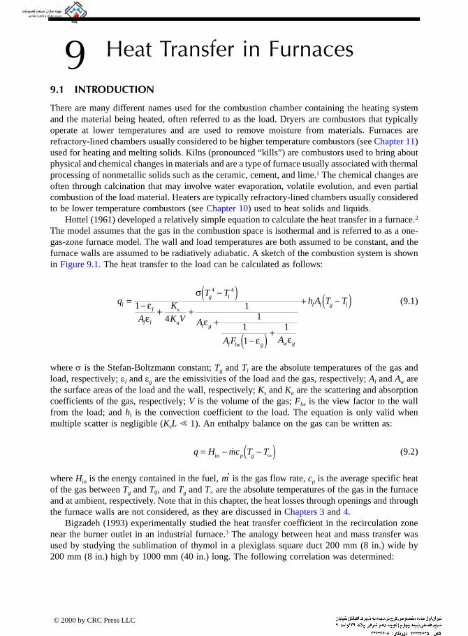
Heat Transfer in Furnaces
99.1 INTRODUCTION
There are many different names used for the combustion chamber containing the heating system and the material being heated, often referred to as the load. Dryers are combustors that typically operate at lower temperatures and are used to remove moisture from materials. Furnaces are refractory-lined chambers usually considered to be higher temperature combustors (see Chapter 11) used for heating and melting solids. Kilns (pronounced “kills”) are combustors used to bring about physical and chemical changes in materials and are a type of furnace usually associated with thermal processing of nonmetallic solids such as the ceramic, cement, and lime.1 The chemical changes are often through calcination that may involve water evaporation, volatile evolution, and even partial combustion of the load material. Heaters are typically refractory-lined chambers usually considered to be lower temperature combustors (see Chapter 10) used to heat solids and liquids.
Hottel (1961) developed a relatively simple equation to calculate the heat transfer in a furnace.2
The model assumes that the gas in the combustion space is isothermal and is referred to as a one-gas-zone furnace model. The wall and load temperatures are both assumed to be constant, and the furnace walls are assumed to be radiatively adiabatic. A sketch of the combustion system is shown in Figure 9.1. The heat transfer to the load can be calculated as follows:
(9.1)
where σ is the Stefan-Boltzmann constant; Tg and Tl are the absolute temperatures of the gas and load, respectively; εl and εg are the emissivities of the load and the gas, respectively; Al and Aw are the surface areas of the load and the wall, respectively; Ks and Ka are the scattering and absorption coefficients of the gas, respectively; V is the volume of the gas; Flw is the view factor to the wall from the load; and hl is the convection coefficient to the load. The equation is only valid when multiple scatter is negligible (KsL 1). An enthalpy balance on the gas can be written as:
(9.2)
where Hin is the energy contained in the fuel, •
m is the gas flow rate, cp is the average specific heat of the gas between Tg and T0, and Tg and T× are the absolute temperatures of the gas in the furnace and at ambient, respectively. Note that in this chapter, the heat losses through openings and through the furnace walls are not considered, as they are discussed in Chapters 3 and 4.
Bigzadeh (1993) experimentally studied the heat transfer coefficient in the recirculation zone near the burner outlet in an industrial furnace.3 The analogy between heat and mass transfer was used by studying the sublimation of thymol in a plexiglass square duct 200 mm (8 in.) wide by 200 mm (8 in.) high by 1000 mm (40 in.) long. The following correlation was determined:
qT T
A
K
K V A
A F A
h A T Tl
g l
l
l l
s
al g
l lw g w g
l l g l=−( )
−+ +
+
−( ) +
+ −( )σεε ε
ε ε
4 4
1
41
11
1
1
q H mc T Tp g= − −( )∞in˙
© 2000 by CRC Press LLC

(9.3)
where dn is the burner nozzle diameter and B is the width of furnace with a square cross-sectional area.
9.2 FURNACES
The choice of the proper furnace type depends on the specific application, as there are many available possibilities. One important consideration is the processing method and whether materials will be processed in batch or continuous mode. Another important consideration is the kind of fuel that will be used.4 Other considerations include the furnace geometry and required temperature range. The processing method and furnace geometry are briefly considered next, while the temperature ranges are considered in Chapters 10 and 11. The two-volume set of books by Trinks and Mawhinney is considered by many to be the bible of furnaces and is a good reference that deals with all aspects of furnaces, including heat transfer and heat recovery.5,6 However, Trinks and Mawhinney (1961, 1967) have specifically limited their definition of industrial furnaces to only those processes that raise the temperature of the material (mainly metals) but do not cause any phase changes (melting or vaporization) or any chemical changes (e.g., calcining). Even with that narrow definition of furnace, they list 61 applicable processes, ranging in material temperatures from 300°F to 3250°F (150°F to 1790°C). Here, industrial furnace is more broadly defined to include processes that not only raise the material temperature, but that may also cause phase changes and chemical reactions. Trinks and Mawhinney also include electric heating, which is not considered here.
DeBellis (1993) studied the heat transfer in furnaces having high-emittance coatings applied to the refractory walls.7 The emittance of the uncoated refractory was approximately 0.5 and the emittance with the coating was approximately 0.8. However, the coating was not stable and the emittance decreased with time. Experiments were conducted both in a small-scale lab furnace and a large-scale metal reheating furnace. In both cases, furnace performance was measured with and without coatings. The results showed that there was no significant change in the rotary hearth reheat furnace efficiency under normal production conditions after the application of the coating.
Khavkin (1996) devoted a significant portion of his book on combustion system design to the use of unlined combustors.8 These unlined chambers are commonly used, for example, in gas turbine engines and internal combustion engines, but they are not commonly used in industrial combustion because of the high temperatures. Khavkin presented a number of designs where no refractory lining is needed, which can save weight, space, and cost. These designs were developed in Russia, but at the present time have not become popular elsewhere because of the technical challenges and potential problems associated with the high heat flux rates from flames to unprotected metal walls.
Lehrman et al. (1998) noted the importance of controlling air infiltration into furnaces.9 This “tramp” air not only reduces thermal efficiency, but in metals production it can also aggravate the problem of surface oxidation (scaling) that lowers product quality and yields. Air infiltration was discussed in Chapter 4 and therefore will not be discussed further here.
FIGURE 9.1 Elevation view of one-gas-zone furnace model.
Nu = −( )⎛⎝⎞⎠0 637 1 8 0 80 78 0 3. Re . Pr .. . d
Bn
© 2000 by CRC Press LLC

9.2.1 FIRING METHOD
There are two main methods used to heat load materials that are usually referred to as direct and
indirect firing. The method chosen is normally dictated by the process requirements. If the material being processed must not come into contact with the combustion products, then indirect firing is used. If there are no such requirements, direct firing is preferred as it is normally more efficient and straightforward.
9.2.1.1 Direct Firing
In a direct-fired furnace, there is nothing between the combustion products generated by the burners and the load, as shown in Figure 9.2. This is the predominant type used in most industrial heating applications and essentially all of the high-temperature processes (see Chapter 11).
In one respect, the heat transfer analysis of direct-fired furnaces is simpler compared to indirect-fired furnaces as there is no intermediate heat-exchanging surface between the flames and the load. However, in another respect, the analysis of the heat transfer to the load is more complicated as convective heat transfer between the flame gases and the load, and therefore fluid flow, must be included. Figure 9.3 shows a cartoon of the heat transfer in a direct-fired furnace using nonluminous flames. As can be seen, the nonluminous radiation from the flame is larger than the luminous radiation. The radiation from the walls to the load is surface radiation. Figure 9.4 shows a cartoon of the heat transfer in a direct-fired furnace from a luminous flame. In that case, the luminous radiation is comparable to, and in many cases more than, the nonluminous flame radiation.
9.2.1.2 Indirect Firing
In an indirect-fired furnace, there is some intermediate heat transfer surface between the combustion products and the load, as shown in Figure 9.5. That surface is commonly some type of ceramic due to the high temperatures, although metals are used in some cases. The surface is designed to
FIGURE 9.2 Elevation view of a direct-fired furnace.
FIGURE 9.3 Heat transfer in a direct-fired furnace from a nonluminous flame (elevation view).
© 2000 by CRC Press LLC

prevent the combustion products from contacting the load and reducing the quality of the finished product. That quality can be reduced in two ways: (1) by chemically altering the product, and (2) by physically changing the surface. An example of the first is in many metallurgical processes, especially heat treating, where the metal product must be heated in a protective atmosphere containing H2, N2, and CO, with only negligible quantities of O2 and H2O, which are detrimental to the quality of the metal during heat treating (see Chapter 10).10 An example of the second type of product quality reduction is in drying a coating or an ink on a web surface in a dryer where the combustion gases could disturb the surface before the coating is dry or the ink is set. Another type of indirect-fired furnace is where the flame gases are separated from the load for either transport or safety reasons. For example, in a process fluid heater, the fluid is transported through metal tubes located inside a furnace. The metal tubes separate the combustion products from the fluid. One reason for the tubes is to transport the fluids at an elevated pressure through the heaters that are fired at approximately atmospheric pressure. Another reason is related to safety, where many of the fluids being heated are hydrocarbons that are potentially explosive if overheated and exposed to enough oxygen.
Two methods are commonly used to separate the combustion products from the load. One is to use open-flame burners but to have a separator, sometimes referred to as a muffle, across the entire combustion space between the flames and the load. Some of the challenges of this method include supporting the separator because of the high temperatures, maximizing the heat transfer from the flames to the separator to optimize the thermal efficiency, and getting a good gas seal around the perimeter of the separator due to thermal expansion. The second method commonly used in industrial combustion applications to separate the exhaust products from the load is to use radiant tube burners (see Chapter 8). In that method, the flame from each individual burner is contained in a ceramic tube. This often improves the overall heat transfer to the separator because of the improved forced convection inside the tube. As with the muffle, supporting long radiant tubes can be a problem as well as the seal between the typically metal burner and ceramic tube.
FIGURE 9.4 Heat transfer in a direct-fired furnace from a luminous flame (elevation view).
FIGURE 9.5 Elevation view of an indirect-fired furnace.
© 2000 by CRC Press LLC

A different challenge compared to the muffle is getting uniform heat flux from the radiant tubes as the hottest gases are produced at the burner end with the coldest gases exiting from the tube.
This can be mitigated through proper design of the radiant tube burner.
The analysis of an indirect-fired furnace may be more complicated than for a direct-fired furnace due to the presence of the heat exchange surface between the flames and the load. The heat transfer from the flames to that surface is normally by both radiation and forced convection. Then, the heat must be conducted through that surface, where it subsequently radiates to the load. This simplifies the analysis of the heat transfer to the load, which is essentially all by radiation.
9.2.1.3 Heat Distribution
The distribution of burners within a furnace has a significant impact on how heat will be transferred. As discussed later in this chapter, the furnace geometry is a large determining factor on where burners will be placed. For example, in a rotary furnace (see Figure 11.15), which is often long and relatively narrow in diameter, a single burner centered on one end of the furnace and firing toward the other end is often the preferred geometry to get proper heat distribution. The desired flame length is often a specific fraction (e.g., half) of the length of the cylinder. In a rectangularly shaped furnace, multiple burners are often used and distributed on one or more walls. In a side-port glass-melting furnace (see Figure 11.20), burners are typically located on two opposite side walls and directly opposed to each other.
The furnace designer, in conjunction with the burner manufacturer, must decide how many burners will be used and where they will be located in the furnace. There are several factors that must be considered. As with most things, economics is an important consideration. It is generally more expensive to use two smaller burners than it is to use one larger burner — not only because of the cost of the burners which is incrementally higher, but also because of the associated extra piping and controls equipment. Another consideration is the physical layout of the furnace structural steel, which limits where burners can be placed in order to avoid steel support members. Still another consideration is the heat transfer distribution within the combustion chamber. Multiple smaller burners often have a more uniform heat distribution pattern than single larger burners, as shown in Figure 9.6 where the size of the flame is proportional to the firing rate. In both cases, the average amount of energy released per unit volume of combustion space is the same; only the distribution of the energy release is different. As can be seen in this example, more uniform heating is usually achieved with more smaller burners, as compared to fewer larger burners.
The actual burner layout is also a function of the burner design and the firing rate of each burner. In certain applications, it may be preferable to have different burners firing at different rates. As an example, Figure 9.7 shows the burner closest to the incoming materials firing the
FIGURE 9.6 Burner distribution effects shown in a plan view of two furnaces with equal total firing rates: (a) three smaller burners vs. (b) one larger burner.
© 2000 by CRC Press LLC
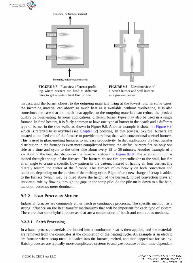
hardest, and the burner closest to the outgoing materials firing at the lowest rate. In some cases, the incoming material can absorb as much heat as is available, without overheating. It is also sometimes the case that too much heat applied to the outgoing materials can reduce the product quality by overheating. In some applications, different burner types may also be used in a single furnace. In fired heaters, it is fairly common to have one type of burner in the hearth and a different type of burner in the side walls, as shown in Figure 9.8. Another example is shown in Figure 9.9, which is referred to as oxy/fuel (see Chapter 12) boosting. In that process, oxy/fuel burners are located at the feed end of the furnace to provide more heat than with conventional air/fuel burners. This is used in glass-melting furnaces to increase productivity. In that application, the heat transfer distribution in the furnace is even more complicated because the air/fuel burners fire on only one side at a time and cycle to the other side about every 15 to 30 minutes. Another example of a variation of the heat distribution in the furnace is shown in Figure 9.10. The scrap aluminum is loaded through the top of the furnace. The burners do not fire perpendicular to the wall, but fire at an angle to create a specific flow pattern in the pattern, instead of having all four burners fire directly toward the center of the furnace. This furnace relies heavily on both convection and radiation, depending on the portion of the melting cycle. Right after a new charge of scrap is added to the furnace (which may be piled above the height of the burners), forced convection plays an important role by flowing through the gaps in the scrap pile. As the pile melts down to a flat bath, radiation becomes more dominant.
9.2.2 LOAD PROCESSING METHOD
Industrial furnaces are commonly either batch or continuous processes. The specific method has a strong influence on the heat transfer mechanisms that will be important for each type of system. There are also some hybrid processes that are a combination of batch and continuous methods.
9.2.2.1 Batch Processing
In a batch process, materials are loaded into a combustor, heat is then applied, and the materials are removed from the combustor at the completion of the heating cycle. An example is an electric arc furnace where scrap metal is loaded into the furnace, melted, and then tapped out for casting. Batch processes are typically more complicated systems to analyze because of their time-dependent
FIGURE 9.7 Plan view of burner profil-ing where burners are fired at different rates to get a certain heat flux profile.
FIGURE 9.8 Elevation view of a hearth burner and wall burners in a process heater.
© 2000 by CRC Press LLC
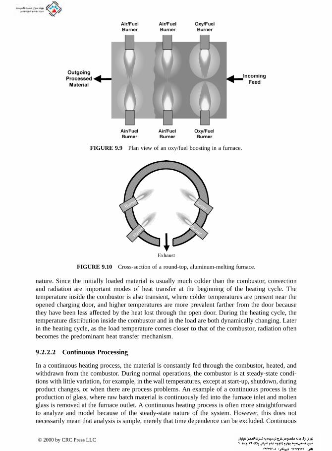
nature. Since the initially loaded material is usually much colder than the combustor, convection and radiation are important modes of heat transfer at the beginning of the heating cycle. The temperature inside the combustor is also transient, where colder temperatures are present near the opened charging door, and higher temperatures are more prevalent farther from the door because they have been less affected by the heat lost through the open door. During the heating cycle, the temperature distribution inside the combustor and in the load are both dynamically changing. Later in the heating cycle, as the load temperature comes closer to that of the combustor, radiation often becomes the predominant heat transfer mechanism.
9.2.2.2 Continuous Processing
In a continuous heating process, the material is constantly fed through the combustor, heated, and withdrawn from the combustor. During normal operations, the combustor is at steady-state condi-tions with little variation, for example, in the wall temperatures, except at start-up, shutdown, during product changes, or when there are process problems. An example of a continuous process is the production of glass, where raw batch material is continuously fed into the furnace inlet and molten glass is removed at the furnace outlet. A continuous heating process is often more straightforward to analyze and model because of the steady-state nature of the system. However, this does not necessarily mean that analysis is simple, merely that time dependence can be excluded. Continuous
FIGURE 9.9 Plan view of an oxy/fuel boosting in a furnace.
FIGURE 9.10 Cross-section of a round-top, aluminum-melting furnace.
© 2000 by CRC Press LLC

heating processes may have a more complicated temperature distribution in the combustor to accommodate the heating of the load. Where a batch combustion process may have fairly uniform
furnace wall temperatures inside the combustor, continuous furnaces may have a wider range of wall temperatures corresponding to the wide spatial temperature differences in the load, which is typically much colder at the feed end than at the discharge end.
Swithenbank et al. (1972) presented a zero-dimensional model for designing continuous com-bustors.11 The model predicted the following primary performance variables: blow-off stability limits, the overall thermal efficiency, the combustion intensity, and the overall pressure loss. Secondary performance variables that were predicted included ignition capability, pressure and temperature effects, pollutant generation, noise, acoustic oscillations, and heat transfer to the wall. The model consisted of interconnected reactors. This is an example of a simplified model used to analyze continuous processes. Other examples are given in Chapter 5.
9.2.2.3 Hybrid Processing
Some processes, like reverberatory furnaces (see Figure 9.12), are hybrids because they have some features of both batch and continuous furnaces. Side-well reverbs often have a provision for continuously feeding new scrap into a well on the side of the furnace, outside of the combustion chamber, so that the door to that chamber does not need to be opened to charge new materials. However, heats are done in discrete cycles, which take on average from 4 to 10 hours, depending on the alloy being made, the furnace conditions, and the operating procedures at the given plant. At the end of the heat, the molten aluminum is tapped out of the furnace through a tap hole and then poured into molds to make ingots for later use, or directly into a specific part like an aluminum wheel. During the tapping portion of the cycle, the burners are normally on a low-fire mode to maintain the heat in the furnace without overheating the aluminum. The heating portion of the cycle is more continuous in nature. The heat transfer inside the furnace varies more during certain parts of the cycle than in others.
Hybrid processes may be more complicated to model and analyze than batch and continuous processes as the hybrid has features of both. One strategy that is often used is to divide the cycle into several subcycles that can be approximated by a quasi steady-state analysis.
9.2.3 HEAT TRANSFER MEDIUM
Another factor that has a significant influence on the heat transfer in the furnace is the medium used to transport the energy from the burners to the load. In industrial combustion, this medium is most commonly a gas, but liquids and solids are also used. In some heat-treating processes, no medium at all is used (vacuum furnaces). The effect of the heat transfer medium on the overall heat transfer in the furnace is briefly considered here.
9.2.3.1 Gaseous Medium
Gases are by far the most common medium used to transport heat from the burners to the load and to the furnace walls. In most direct-fired processes, the combustion products themselves transport heat to the load by forced convection. The actual rate of heat transfer depends on the flow geometry (gas velocity, how the gas flows over the load, and the shape of the load), the temperatures of both the gases and the load, and the gas composition. Processes are often specifically designed to maximize this convective heat transfer. For example, in a counter-flow rotary kiln, the combustion products flow in one direction while the load flows in the other direction to maximize the temper-ature difference between the combustion products and the load over the entire length of the kiln. Another example is in heat-treating furnaces where the furnace atmosphere is recycled and blown onto the parts being treated to improve temperature uniformity and to reduce the heating cycle time. Certain gases (CO2, H2O, SO2, CH4, etc.) also transfer heat to the load and to the furnace
© 2000 by CRC Press LLC
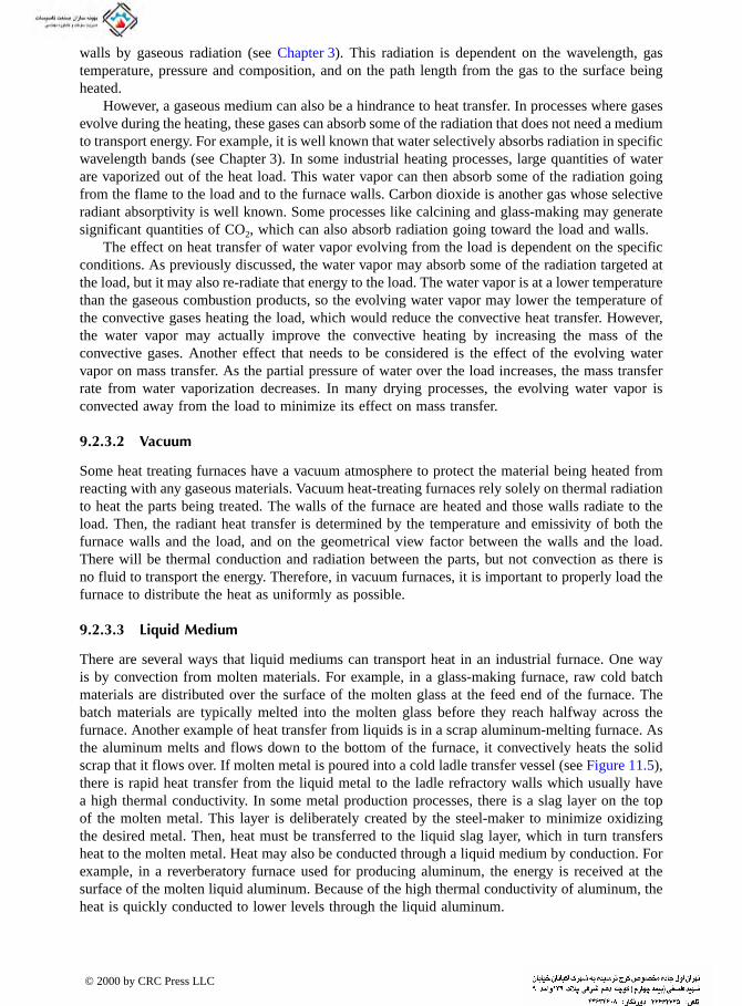
walls by gaseous radiation (see Chapter 3). This radiation is dependent on the wavelength, gas temperature, pressure and composition, and on the path length from the gas to the surface being
heated.
However, a gaseous medium can also be a hindrance to heat transfer. In processes where gases evolve during the heating, these gases can absorb some of the radiation that does not need a medium to transport energy. For example, it is well known that water selectively absorbs radiation in specific wavelength bands (see Chapter 3). In some industrial heating processes, large quantities of water are vaporized out of the heat load. This water vapor can then absorb some of the radiation going from the flame to the load and to the furnace walls. Carbon dioxide is another gas whose selective radiant absorptivity is well known. Some processes like calcining and glass-making may generate significant quantities of CO2, which can also absorb radiation going toward the load and walls.
The effect on heat transfer of water vapor evolving from the load is dependent on the specific conditions. As previously discussed, the water vapor may absorb some of the radiation targeted at the load, but it may also re-radiate that energy to the load. The water vapor is at a lower temperature than the gaseous combustion products, so the evolving water vapor may lower the temperature of the convective gases heating the load, which would reduce the convective heat transfer. However, the water vapor may actually improve the convective heating by increasing the mass of the convective gases. Another effect that needs to be considered is the effect of the evolving water vapor on mass transfer. As the partial pressure of water over the load increases, the mass transfer rate from water vaporization decreases. In many drying processes, the evolving water vapor is convected away from the load to minimize its effect on mass transfer.
9.2.3.2 Vacuum
Some heat treating furnaces have a vacuum atmosphere to protect the material being heated from reacting with any gaseous materials. Vacuum heat-treating furnaces rely solely on thermal radiation to heat the parts being treated. The walls of the furnace are heated and those walls radiate to the load. Then, the radiant heat transfer is determined by the temperature and emissivity of both the furnace walls and the load, and on the geometrical view factor between the walls and the load. There will be thermal conduction and radiation between the parts, but not convection as there is no fluid to transport the energy. Therefore, in vacuum furnaces, it is important to properly load the furnace to distribute the heat as uniformly as possible.
9.2.3.3 Liquid Medium
There are several ways that liquid mediums can transport heat in an industrial furnace. One way is by convection from molten materials. For example, in a glass-making furnace, raw cold batch materials are distributed over the surface of the molten glass at the feed end of the furnace. The batch materials are typically melted into the molten glass before they reach halfway across the furnace. Another example of heat transfer from liquids is in a scrap aluminum-melting furnace. As the aluminum melts and flows down to the bottom of the furnace, it convectively heats the solid scrap that it flows over. If molten metal is poured into a cold ladle transfer vessel (see Figure 11.5), there is rapid heat transfer from the liquid metal to the ladle refractory walls which usually have a high thermal conductivity. In some metal production processes, there is a slag layer on the top of the molten metal. This layer is deliberately created by the steel-maker to minimize oxidizing the desired metal. Then, heat must be transferred to the liquid slag layer, which in turn transfers heat to the molten metal. Heat may also be conducted through a liquid medium by conduction. For example, in a reverberatory furnace used for producing aluminum, the energy is received at the surface of the molten liquid aluminum. Because of the high thermal conductivity of aluminum, the heat is quickly conducted to lower levels through the liquid aluminum.
© 2000 by CRC Press LLC

9.2.3.4 Solid Medium
There are several ways that heat can be transferred through a solid medium in an industrial furnace.
One method is by luminous radiation produced by solid soot particles generated in the flame (see Chapter 3). Another method is by thermal conduction between contacting solid parts. For example, in a vacuum furnace, energy is received at the outer boundaries of the pile of parts. Then heat is conducted into the parts by thermal conduction between the parts in contact with each other. Solid parts can also transfer heat by radiating to each other. Although not considered here, in a fluidized bed combustor, heat is transferred by circulating suspended solid particles.
9.2.4 GEOMETRY
The geometry refers to both the shape and the size of the combustion chamber. An important parameter that determines the heat loss from a combustor is the external surface area. Heat is lost by both convection and radiation from the outside surface walls. Combustor geometries with higher surface areas will normally have higher losses than those with lower surface areas, assuming everything else is equivalent. One way that combustors are designed is based on the heat release per unit of combustor volume (e.g., kW/m3 or Btu/hr-ft3). It is then possible to compare the ratio of the surface area to the volume for different geometries:
(9.4)
The higher the SV ratio, the higher the proportion of heat loss for that combustor design. A spherical combustor would have the following surface area to volume ratio:
(9.5)
where r is the radius of the sphere. This shows that the larger the sphere, the lower the SVsphere , which normally means proportionally lower heat losses. Similarly, a cubical combustor would have the following surface area to volume ratio:
(9.6)
where l is the length of each side of the cube. As the cube size increases, SVcube decreases, which again should result in proportionately lower heat losses (see Figure 9.11). This implies that larger furnaces should have proportionally lower heat losses and therefore be more thermally efficient than smaller furnaces, all other factors being equivalent. This is true in most cases, although real industrial processes are often more complicated than strictly considering the size. For example, in a batch process, loading and unloading the furnace may take proportionately more or less time for a larger furnace, depending on the material handling methods and downstream processes.
It is also instructive to compare the relative shapes of combustors and their impact on heat losses. For the sake of comparison, the volume of the furnace will be held constant as the heat release per unit furnace volume will be assumed to be fixed. This would not be strictly true if the heat losses varied for different furnace geometries as more heat would be required for furnaces with higher heat losses. However, the heat losses for a well-insulated furnace are commonly relatively small, so fixing the furnace volume is reasonable to compare surface area effects. The base case will be a cubical furnace with the length of each side equal to 1 unit (l = 1). Then, the
SV = surface areavolume
SVr
r rsphere = π
π=4
43
32
3
SVll lcube = =6 62
3
© 2000 by CRC Press LLC

volume of that cube would be 1 unit3 and the surface area would be 6 unit2, with an SVcube = 6 unit–1. For a spherical combustor with an equal volume of 1 unit3, the radius would be r = 0.62 units. Then the SVsphere would be 4.8 unit–1. The ratio of surface to volume ratios for the sphere to the cube (SVsphere /SVcube) equals 0.81. This means that a cubical furnace would normally have proportionally higher heat losses than a spherical furnace, for equal volumes. However, it is not as practical to build a spherical furnace, compared to a cubical furnace.
One can also compare a rectangular furnace to a cubical furnace to see how the heat loss would be affected. Again assume a base case of a cubical furnace with a unit volume. Choose a rectangular furnace that has two sides of equal length l1 with the remaining side twice as long or l2 = 2l1, also with a volume of 1 unit3. Then l1 would be 0.79 units to get an equivalent volume to the cube and the SVrectangular = 6.3. The ratio of the surface to volume ratios for this rectangular shape and the cube of equal volume (SVrectangular /SVcube) equals 1.05. This indicates that the heat loss should be higher for a rectangular furnace compared to a cubical furnace of equal volume and shows a comparison of the cubical, spherical, and rectangular furnaces that all have a unit volume of 1 unit3. Figure 9.12 shows a scale drawing with a comparison of the three furnace geometries of equal volume.
There are numerous combustor geometries in industrial combustion processes, many of which are considered in other sections of this book (especially Chapters 10 and 11). Only a few repre-sentative geometries are considered next to study their effects on heat transfer.
9.2.4.1 Rotary Geometry
Rotary kilns are typically cylindrical, refractory-lined vessels that are used to heat solid materials like cement, lime, and scrap aluminum. They typically have high length-to-diameter ratios, are slightly inclined from the horizontal, and rotate. The material is fed in at the higher end and exits at the lower end of the kiln. This geometry is normally characterized by a single burner located in or near the center of one end of the kiln and firing parallel to the axis of the kiln. In counter-current rotary kilns, the material is fed in on the opposite end of the burner. In co-current rotary kilns, the material inlet and the burner are at the same end. The flames are usually round — to match the cylindrical furnace geometry and to transfer heat uniformly around the furnace. Longer flame lengths are often desired to get better heat transfer coverage over a longer length of the furnace.
FIGURE 9.11 Surface area-volume ratio (SV) for a cubical furnace as a function of the length of each side of the cube.
© 2000 by CRC Press LLC

ubical, spherical, and rectangular furnaces with volumes of 1 unit3.
FIGURE 9.12 C
© 2000 by CRC Press LLC

The heat transfer in a rotary kiln is unique compared to other geometries because it transfers heat under the load, as well as on top. The flame transfers heat to the load and to the exposed furnace walls. Because the furnace rotates, the heated walls rotate under the load and transfer heat to the bottom of the load by thermal conduction. In addition, the solids typically tumble inside the kiln, which constantly exposes new material to the heat source. Tumbling the load and heating from below help increase the efficiency of this process.
Jenkins and Moles (1981) developed an analytical model to predict the heat transfer from a large flame in a rotary kiln.12 Hottel’s zone method was used to simulate radiation heat transfer in the kiln. The model results compared reasonably well with experimental data. Boateng (1997) numerically studied the heat transfer in rotary kilns processing a granular bed.13 Figure 9.13 shows a sketch of a rotary kiln with 12% loading of a granular material. Two distinct regions are present in the cross-section of the kiln, which are referred to as the freeboard and the bed. The gases flow in the freeboard space and the solid material occupies the bed. The bed material is heated from above by radiation from the flame and the upper kiln walls, and by convection from the combustiongases. The bed is also heated from below by thermal conduction from the lower refractory kiln
FIGURE 9.13 Schematic of a cross-sectional view of granular flow in a rotary kiln, including the bed behavior at 12% loading. (Courtesy of ASME, New York.13 With permission.)
© 2000 by CRC Press LLC

wall in contact with the bed. In the figure, six different bed behaviors are given, depending on the bed rotational Froude number, which is defined as:
(9.4)
where ω is the angular velocity of the kiln (sec–1), r is the cylinder radius (m), and g is the acceleration due to gravity (m/sec2).
9.2.4.2 Rectangular Geometry
The rectangular shape is one of the workhorses in industrial combustion. One example of a horizontally fired rectangular furnace is the reverb furnace, commonly used in aluminum melting, which is shown in Figure 9.14. An example of a vertically fired rectangular furnace is the cabin heater. Figure 9.15 shows several different burner arrangements that are used in cabin heaters, depending on both the width of the cabin and the size of the burners. If more than two rows are used in a cabin-type heater, the inner rows of burners may be fired at full rate, while the outer burners may be fired at a reduced rate to prevent overheating the outer walls.
As with other furnace geometries, much of the energy received by the load comes from surface radiation from the refractory-lined furnace walls. In most cases, there is very little heat transfer to or from the furnace below the level of the material loading. The objective is normally to make the furnace as adiabatic as possible to minimize heat losses and to maintain the material temperature.
As discussed above, burners may be positioned in a variety of locations, depending on the process. In some process heaters, there are burners in the floor that fire upward. In glass furnaces, burners are located in the side walls that fire parallel to the floor and roof. In reverberatory furnaces used to melt aluminum, burners are located in the side wall, but are typically angled down toward the load. In reformers, burners are located in the roof and fire downward.
9.2.4.3 Ladle Geometry
Ladles are commonly used to transport molten metal from melting furnaces to casting stations in metal production facilities (see Chapter 11). They are refractory-lined, vertical cylindrical vesselsthat are closed at one end and usually open at the top. Many metal-melting operations are batch
FIGURE 9.14 Sketch of a reverb furnace.
Fr = ω2rg
© 2000 by CRC Press LLC

processes. When a heat is ready to be tapped from the furnace, the molten metal is poured into a ladle and transported, usually via an overhead crane, to the casting station. A major challenge with ladles is to minimize the amount of metal that solidifies on the relatively cold (prior to receiving the molten metal) ladle wall. One way to minimize the thermal gradient between the ladle wall and the molten metal is to preheat the ladle with a burner just prior to pouring the metal into the ladle. This preheating is done in a preheat stand as shown in Figure 9.16. The burner wall may have an opening above the burner that acts as the exhaust flue. In some cases, the gap between the ladle and the burner wall acts as the vent. The top edge of a ladle is often far from flat due to what are called “skulls,” which are frozen pieces of molten metal around the rim. This makes it difficult to get a tight seal between the burner wall and the ladle.
From a heat transfer perspective, ladles are somewhat unique in that when they are used to transport molten metal, the heat transfer is essentially all by convection and conduction. There is very little radiation heating because the vessel is typically filled close to the top. If the vessel is not covered, then heat is lost by radiation from the top layer of molten metal. When the ladle is being preheated with a burner, the heat transfer is primarily by radiation with some convection.
FIGURE 9.15 Burner B arrangement in the floor of cabin heaters (plan view): (a) single row of burners in a narrower heater; (b) two rows of staggered burners in a slightly wider heater; and (c) two rows of parallel burners in an even wider heater.
FIGURE 9.16 Ladle preheater stand with empty ladle on its side and temporary burner wall against ladle.
© 2000 by CRC Press LLC

9.2.4.4 Vertical Cylindrical Geometry
Vertical cylindrical (VC) furnaces are commonly used in the chemical and petrochemical industries for heating hydrocarbon fluids. These furnaces usually have burners in the floor of the furnace, either centered or arranged in a circle pattern (see Figure 9.17), and fire straight upward. The tubes carrying the fluids are vertical and against the cylinder wall. The heat transfer to the tubes is primarily by radiation from both the VC walls and from the flames.
Maesawa et al. (1972) measured the radiation heat flux from industrial residual oil flames in a VC furnace.14 The peak emissivity and radiant heat flux were found at approximately one-third the length of the furnace away from the burner. Steward et al. (1972) made heat transfer measure-ments in a small VC test furnace where the walls were cooled by an oil.15 Radiative and total heat fluxes were measured with a custom-built radiometer. A single vertical burner firing propane with 20% excess air was used. Sample radiative heat flux results are shown in Figure 9.18.
9.2.5 FURNACE TYPES
A few common types of furnaces are briefly discussed in this chapter section. Although there are many types of furnaces, the ones chosen for discussion here have significant differences in the heat transfer of the process. These are representative of a variety of furnaces that are often variations of those discussed here.
9.2.5.1 Reverberatory Furnace
A reverberatory or “reverb” furnace (see Figure 9.14) is a rectangular refractory-lined box that is typically used to process non-ferrous metals. Burners are located in one wall or in the roof. The exhaust may be in the roof or on one of the walls, often in between the burners. Reverberatory furnaces are operated as semicontinuous processes, as discussed above. The burners are used primarily to heat the refractory walls of the reverb. The hot walls then re-radiate or reverberate the energy to the load inside the furnace. In the case of aluminum, the surface emissivity of molten aluminum ranges from 0.004 to 0.55.16 However, molten aluminum readily forms a slag layer on the surface consisting of aluminum oxide, which has an emissivity of 0.11 to 0.19. This results in poor heat transfer qualities as the primary mode of heat transfer is radiation to the surface. Therefore, the dross layer thickness should be minimized. The furnace is designed to compensate for this by having a high bath surface area-to-melt ratio, compared to some other furnace designs.
FIGURE 9.17 Burner B arrangement in the floor of vertical cylindrical furnaces (plan view): (a) small-diameter furnace with a single centered burner, and (b) larger diameter furnace with four burners symmetrically arranged at a radius from the centerline.
© 2000 by CRC Press LLC

There are two common methods for loading reverbs: direct charging and indirect charging. In direct charging, a charging door to the combustion chamber is opened and the load is directly placed into the combustion chamber. The burners in that chamber normally go to a low-fire mode during the charging and then go back to a high-fire mode after the door has been closed. This method of operation is less efficient as the heat losses from the opened door are substantial. This is also much more of a batch-type operation because of the discrete load charges.
Indirect charge reverbs are often more efficient and are closer to a continuous process because of the charging method, although they are still batch processes because there are discrete times when the load is tapped from the furnace. The load is commonly charged into a chamber attached to the side of the combustion chamber, often referred to as a side well. This type of reverb is called a side-well reverb. These are more thermally efficient as no doors need to be opened on the combustion chamber. The solid load is placed into the side well and then carried into the combustion chamber by circulating molten metal.
Forced convection also plays an important role in reverbs, especially during the initial part of the heating cycle after a new charge has been added directly into the combustion chamber. High-velocity burners direct hot combustion products toward the load to enhance convective heating. As the solids melt, radiation becomes more and more important. Thermal conduction also plays an important role in reverbs since the heat transferred to the surface of the load must be conducted down into the load. In the case of aluminum, which has a very high thermal conductivity, the heat is conducted rapidly through the load, resulting in a more uniform temperature distribution.
Reverb furnaces also have large wall surface areas to maximize the heat transfer to the bath. This also increases the wall losses. For furnaces that do not have special submerged pumps to circulate the molten metal, the bath depth is often shallow to ensure good heat transfer through the bath. For furnaces with pumps, the bath depth is usually thicker because the increased mixing enhances the heat transfer through the bath. It is not uncommon for reverbs to have some type of heat recuperation for preheating the incoming combustion air, to improve the thermal efficiency.
FIGURE 9.18 Radiative flux as a function of axial distance and firing rate for propane firing in a vertical cylindrical furnace. (Courtesy of the Combustion Institute, Pittsburgh, PA.15 With permission.)
© 2000 by CRC Press LLC

9.2.5.2 Shaft Kiln
A vertical shaft kiln is shown in Figure 9.19. It acts like a counterflow heat exchanger, where the hot exhaust products from the burners located at the bottom flow upward while the incoming cold materials flow downward. These vertical shaft kilns have been used for years for calcining limestone and for manufacturing cement. The heat transfer is fairly unique compared to other industrial heating processes because of the vertical counterflow of materials going down and exhaust products going up. Convection plays a more important role and wall radiation is much less important, compared to many other processes. Thermal conduction is also more important because of the direct contact between moving layers of materials. Feeding solid materials from the top of the furnace is a unique aspect of this furnace configuration.
9.2.5.3 Rotary Furnace
A rotary kiln is shown in Figure 9.20. The raw materials are fed in at the top of the inclined, slowly rotating cylinder and exit at the opposite end. These are often continuous processes where raw material is continuously fed in one end and treated materials exit at the other end. The raw materials are solid materials that are often granular in composition so that they can easily flow through the kiln. These kilns also normally operate as counterflow heat exchangers with the burner at the discharge end and the incoming feed at the opposite end. However, there are also co-flow versions of this type of kiln. Rotary kilns are used for processing bulk materials like cement, lime, and other minerals. Large cement kilns can be up to 20 ft (6 m) in diameter and 500 ft (160 m) in length.
FIGURE 9.19 Elevation view of a vertical shaft kiln. (Courtesy of CRC Press, Boca Raton, FL.1)
© 2000 by CRC Press LLC
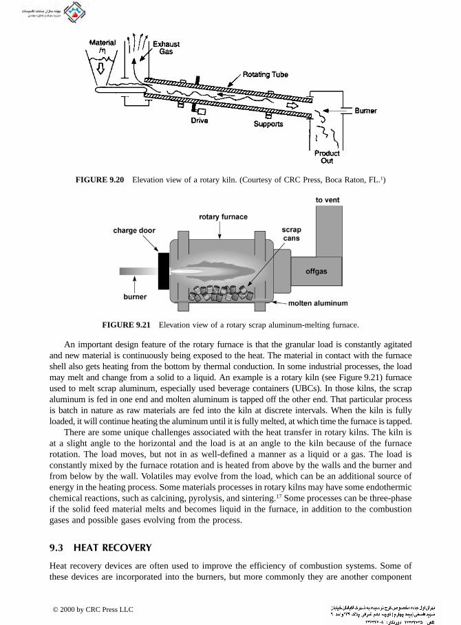
An important design feature of the rotary furnace is that the granular load is constantly agitated and new material is continuously being exposed to the heat. The material in contact with the furnace shell also gets heating from the bottom by thermal conduction. In some industrial processes, the load may melt and change from a solid to a liquid. An example is a rotary kiln (see Figure 9.21) furnace used to melt scrap aluminum, especially used beverage containers (UBCs). In those kilns, the scrap aluminum is fed in one end and molten aluminum is tapped off the other end. That particular process is batch in nature as raw materials are fed into the kiln at discrete intervals. When the kiln is fully loaded, it will continue heating the aluminum until it is fully melted, at which time the furnace is tapped.
There are some unique challenges associated with the heat transfer in rotary kilns. The kiln is at a slight angle to the horizontal and the load is at an angle to the kiln because of the furnace rotation. The load moves, but not in as well-defined a manner as a liquid or a gas. The load is constantly mixed by the furnace rotation and is heated from above by the walls and the burner and from below by the wall. Volatiles may evolve from the load, which can be an additional source of energy in the heating process. Some materials processes in rotary kilns may have some endothermic chemical reactions, such as calcining, pyrolysis, and sintering.17 Some processes can be three-phase if the solid feed material melts and becomes liquid in the furnace, in addition to the combustion gases and possible gases evolving from the process.
9.3 HEAT RECOVERY
Heat recovery devices are often used to improve the efficiency of combustion systems. Some of these devices are incorporated into the burners, but more commonly they are another component
FIGURE 9.20 Elevation view of a rotary kiln. (Courtesy of CRC Press, Boca Raton, FL.1)
FIGURE 9.21 Elevation view of a rotary scrap aluminum-melting furnace.
© 2000 by CRC Press LLC

in the combustion system, separate from the burners. These heat recovery devices incorporate some type of heat exchanger, depending on the application. The two most common types have been recuperators and regenerators, which are discussed next. The classifications of these heat exchangers are shown in Figure 9.22. Gas recirculation effects on heat transfer are also considered in this chapter section.
9.3.1 RECUPERATORS
A recuperator is a low- to medium-temperature (up to about 1300°F, or 700°C), continuous heat exchanger that uses the sensible energy from hot combustion products to preheat the incoming combustion air. These heat exchangers are commonly counterflow, where the highest temperatures for both the combustion products and the combustion air are at one end of the exchanger and the coldest temperatures are at the other end. Lower temperature recuperators are normally made of metal, while higher temperature recuperators may be made of ceramics. Recuperators are typically used in lower temperature applications because of the limitations of the metals used to construct these heat exchangers.
9.3.2 REGENERATORS
A regenerator is a higher temperature, transient heat exchanger used to improve the energy efficiency of higher temperature heating and melting processes, particularly in the high-temperature processing industries like glass production. Regenerators are sometimes referred to as “capacitive heat exchang-ers” and are mainly used in gas/gas heat recovery.18 In a regenerator, energy from the hot combustion products is temporarily stored in a unit constructed of some type of packing, such as firebricks. This energy is then used to heat the incoming combustion air during a given part of the firing cycle up to temperatures in excess of 2400°F (1300°C).19
Regenerators constructed of a honeycomb of firebricks are often called a chequer work or simply a chequer. Other packing materials can also be used, depending on the application. The packing material must be able to tolerate the thermal shock of constant thermal cycling and may need to withstand a potentially corrosive environment, such as in the manufacturing of glass. Many different patterns, such as the “square chimney” or “closed basket weave” are used in arranging the packing material, depending on the material and the pressure drop requirements. An additional
FIGURE 9.22 Heat exchanger classifications. (Courtesy of CRC Press, Boca Raton, FL.18)
© 2000 by CRC Press LLC

requirement is that the regenerators should either not be easily plugged or should be easy to clean if they do get plugged — in order to minimize downtime.
Regenerators are normally operated in pairs because of the normal requirement for a continuous stream of preheated air. During one part of the cycle, the hot combustion gases are flowing through one of the regenerators and heating up the refractory bricks (known as the “hot blow” or “hot period”), while the combustion air is flowing through and cooling down the refractory bricks in the second regenerator (known as the “cold blow” or “cold period”). Both the exhaust gases and the combustion air directly contact the bricks in the regenerators, although not both at the same time since each is in a different regenerator at any given time. After a sufficient amount of time (usually from 5 to 30 min), the cycle is reversed so that the cooler bricks in the second regenerator are then reheated, while the hotter bricks in the first regenerator exchange their heat with the incoming combustion air. A reversing valve is used to change the flow from one gas to another in each regenerator. This is shown schematically in Figure 9.23.
In the more efficient counter-flow regenerator operation, the hot gases pass through the regen-erator in the opposite direction to the cold gases that go through the regenerator; while in the less efficient parallel flow operation, both the hot and cold gases pass through the regenerator in the same direction.20 There are also rotary regenerators that are single units that use the hot combustion products to preheat a rotating ring which is then used to preheat the incoming combustion air. The ring rotates so that it is continually heating and cooling. Then, only a single regenerator is needed to provide a continuous stream of preheated air. The basic problem with rotary regenerators is that they are not completely gas-tight so that exhaust products leak into the combustion air stream and vice versa.
FIGURE 9.23 Schematic of a fixed-bed regenerator. (Courtesy of CRC Press, Boca Raton, FL.20)
© 2000 by CRC Press LLC
Miyami et al. (1998) described the heat transfer characteristics of a rotary regenerative com-bustion system where the heat from the exhaust products was used to preheat the incoming
combustion air in a single burner.21 Their model, which included both convection and radiation, was able to predict the performance of a rotary regenerative air preheating system within 10%. Radiation was much less than forced convection in this system. The emissivity of the heat accu-mulator was assumed to be 1.0. The new RRX system was designed to eliminate some potential disadvantages of high-frequency (every 20 to 30 seconds) regenerative systems, including:
• Furnace pressure fluctuations due to repeated ignition and extinguishment of the burner• Reliability concerns for the changeover valve, which might actuate as many as a million
times in a year• Higher than desired NOx emissions• Large space requirements because of the size of the regenerators and the fact that
traditional regenerative burners must be installed in pairs
9.3.3 GAS RECIRCULATION
There are two common types of gas recirculation in industrial combustors: furnace and flue gas. These are briefly considered next.
9.3.3.1 Flue Gas Recirculation
Flue gas recirculation is schematically shown in Figure 1.9. In this process, the exhaust products are taken out of the flue and recirculated back into the furnace, often through the burners. The recirculation requires an external, high-temperature fan to move the gases and the associated high-temperature ductwork to transport the gases. There are two common reasons for employing this type of recirculation. In the past, the major reason was for heat recovery. The hot combustion exhaust products were given a second chance to transfer their energy to a lower temperature heat load. A more recent reason to use this technology is to reduce NOx emissions. Although the recirculated gases may be hot, they are not nearly as hot as the flame gases, so the recirculated gases actually cool the flame. The reduced flame temperature reduces NOx emissions, which are highly temperature dependent.
This type of recirculation can have a significant impact on the heat transfer in the furnace. One primary effect is that the forced convection heat transfer is often increased due to the added mass of gases flowing through the furnace and the higher overall gas velocities. However, the forced convection may be tempered by the lower overall gas temperature by diluting the hot flame products with colder flue gases. Since the thermal efficiency increases for nearly all processes employing flue gas recirculation, the overall effect on convection is to increase it.
9.3.3.2 Furnace Gas Recirculation
This is a related process where combustion products are recirculated inside the combustor. An example of a burner designed to produce this type of recirculation is shown in Figure 8.48. There, the high-velocity core jet of pure oxygen induces furnace gases to flow into the burner to dilute the flame temperature. Other burner designs use the flow inside the furnace to recirculate the exhaust products back toward the burners. This technique also tends to improve thermal efficiencies and reduce NOx emissions, but to a lesser extent compared to flue gas recirculation. However, the capital and operating costs are also less since no external fan and ductwork are required. Therefore, the technique chosen is a balance of economics and desired benefits. The heat transfer in the furnace is similarly affected as with flue gas recirculation, but the magnitude of the change is usually smaller.
© 2000 by CRC Press LLC

REFERENCES
1. G.L. Shires, Kilns, in International Encyclopedia of Heat & Mass Transfer, G.F. Hewitt, G.L. Shires,
and Y.V. Polezhaev, Eds., CRC Press, Boca Raton, FL, 1997, 651-653.2. H.C. Hottel, The Melchett Lecture for 1960: Radiative Transfer in Combustion Chambers, J. Inst.
Fuel, 34, 220-234, 1961.3. E. Bigzadeh, An experimental determination of the heat transfer coefficient in the recirculation zone
of an industrial furnace with a square cross-section, in Heat Transfer in Fire and Combustion Systems — 1993, B. Farouk, M. Pinar Menguc, R. Viskanta, C. Presser, and S. Chellaiah, Eds., New York, ASME HTD-Vol. 250, 185-189, 1993.
4. A.J. Johnson and G.H. Auth, Fuels and Combustion Handbook, first edition, McGraw-Hill, New York, 1951.
5. W. Trinks and M.H. Mawhinney, Industrial Furnaces, Vol. 1, 5th edition, Wiley, New York, 1961.6. W. Trinks and M.H. Mawhinney, Industrial Furnaces, Vol. 2, 4th edition, Wiley, New York, 1967.7. C.L. DeBellis, Evaluation of high-emittance coatings in a large industrial furnace, in Heat Transfer
in Fire and Combustion Systems — 1993, B. Farouk, M. Pinar Menguc, R. Viskanta, C. Presser, and S. Chellaiah, Eds., ASME HTD-Vol. 250, New York, 1993, 190-198.
8. Y.I. Khavkin, Combustion System Design: A New Approach, PennWell Books, Tulsa, OK, 1996.9. A. Lehrman, C.D. Blumenschein, D.J. Doran, and S.E. Stewart, Steel plant fuels and water require-
ments, in The Making, Shaping and Treating of Steel, 11th edition, Steelmaking and Refining Volume, R.J. Fruehan, Ed., AISE Steel Foundation, Pittsburgh, PA, 1998, 311-412.
10. H.S. Kurek, M. Khinkis, W. Kunc, A. Touzet, A. de La Faire, T. Landais, A. Yerinov, and O. Semernin, Flat radiant panels for improving temperature uniformity and product quality in indirect-fired furnaces, Proc. 1998 International Gas Research Conf., Vol. V: Industrial Utilization, D.A. Dolenc, Ed., Gas Research Institute, Chicago, 1998, 15-23.
11. J. Swithenbank, I. Poll, M.W. Vincent, and D.D. Wright, Combustion design fundamentals, Fourteenth Symposium (International) on Combustion, The Combustion Institute, Pittsburgh, PA, 1972, 627-638.
12. B.G. Jenkins and F.D. Moles, Modelling of heat transfer from a large enclosed flame in a rotary kiln, Trans. Inst. Chem. Eng., 59(1), 17-25, 1981.
13. A.A. Boateng, On flow induced kinetic diffusion and rotary kiln bed burden heat transfer, in Proc. 32nd National Heat Transfer Conf., Vol. 3: Fire and Combustion Systems, L. Gritzo and J.-P. Del-planque, Eds., New York, ASME HTD-Vol. 341, 183-191, 1997.
14. M. Maesawa, Y. Tanaka, Y. Ogisu, and Y. Tsukamoto, Radiation from the luminous flames of liquid fuel jets in a combustion chamber, Twelfth Symposium (International) on Combustion, The Combustion Institute, Pittsburgh, PA, 1968, 1229-1237.
15. F.R. Steward, S. Osuwan, and J.J.C. Picot, Heat-transfer measurements in a cylindrical test furnace, Fourteenth Symposium (International) on Combustion, The Combustion Institute, Pittsburgh, PA, 1972, 651-660.
16. E. Lange, Stack melter or reverb … choosing a new central melter, Die Casting Engineer, 38(4), 12-16, 1994.
17. J.R. Ferron and D.K. Singh, Rotary kiln transport processes, AIChE J., 37(5), 747-758, 1991.18. R.J. Brogan, Heat exchangers, in International Encyclopedia of Heat & Mass Transfer, G.F. Hewitt,
G.L. Shires, and Y.V. Polezhaev, Eds., CRC Press, Boca Raton, FL, 1997, 546-550.19. Y. Suzukawa, S. Sugiyama, and I. Mori, Heat transfer improvement and NOx reduction in an industrial
furnace by regenerative combustion system, Proc. 31st Intersociety Energy Conversion Eng. Conf., Institute of Electrical & Electronics Eng., Washington, D.C., August, 1996, 804-809.
20. A.J. Willmot, Regenerative heat exchangers, in International Encyclopedia of Heat & Mass Transfer, G.F. Hewitt, G.L. Shires, and Y.V. Polezhaev, Eds., CRC Press, Boca Raton, FL, 1997, 944-953.
21. H. Miyami, H. Kaji, Y. Hirose, and N. Arai, Heat transfer characteristics of a rotary regenerative combustion system (RRX), Heat Transfer — Japanese Research, 27(8), pp. 584-596, 1998.
© 2000 by CRC Press LLC

Lower Temperature Applications
1010.1 INTRODUCTION
The designation “lower temperature application” is somewhat relative, but here it refers to processes with furnace temperatures below about 2200°F (1200°C). The major applications considered in this chapter include ovens and dryers, fired heaters, and heat-treating furnaces. In general, the dominant heat transfer mechanisms are radiation and forced convection, depending on the specific application. This is in contrast to higher temperature applications that are dominated almost exclusively by thermal radiation.
10.2 OVENS AND DRYERS
An important consideration for the choice of the type of oven or dryer for a specific application depends on whether direct or indirect heating is needed.1 Direct heating means the product is exposed directly to the flame (see Figure 10.1), while indirect heating means the products of combustion do not come in contact with the material being heated (see Figure 10.2). In indirect heating, an intermediate carrier or type of heat exchanger is used to transfer the heat. Normally, an intermediate medium between the flame and the load reduces the thermal efficiency compared to direct heating. The most common reason for keeping the exhaust products separate from the heat load is for product quality, wherein the product could be contaminated by the exhaust gases. Another reason is that the product may be emitting combustible volatile vapors that could be ignited if they come into contact with open flames. Still another reason might be that exhaust gases could carry fine particles from the load out of the combustor. These particles would then have to be scrubbed out of the exhaust before the exhaust enters the atmosphere. That means that not only are the raw material costs higher, but there is also the added cost of removing the unused raw materials in the exhaust. As expected, the heat transfer mechanisms will be different, depending on the type of heating used in a given process.
10.2.1 PREDRYER
Predryers are used in some applications prior to the final drying of the product. An example of this type of application is the use of infrared (IR) burners to set the dyes in the dyeing of fabrics in textile manufacturing.2 After the dyes are applied to the fabric, they must be set prior to contact with the dryer; otherwise, the dyes will migrate to drier areas of the fabric, which reduces the quality of the textile. The IR burners in the predryer are used to rapidly set the dyes without the need to contact the material, as would be the case with, for example, a drum dryer.
Another example of predrying is in the paper industry where IR burners are installed after the coating machine and are used to set the coatings on the paper prior to the paper contacting a steam cylinder drum dryer used to complete the drying (see section 10.2.2).3 The IR predryer is primarily used to increase productivity and improve the paper coating quality. The productivity is increased because of the added heat. The quality is improved because the IR energy does not disturb the coating as convection or conduction heat transfer methods would, which lets the coating set on the paper prior to contact with the steam cylinder, which relies on thermal conduction heat transfer. Figure 10.3 shows the typical spectral radiant transmissivity for uncoated paper. The paper is less absorbent at longer wavelengths and more absorbent at shorter wavelengths. Since IR burners
© 2000 by CRC Press LLC

typically have their peak radiant output at wavelengths less than 3 µm, this leads to good thermal efficiencies because the paper is highly absorbent to those wavelengths. Mottle is a measure of thequality of the finished paper product and refers to the finish. Higher mottle means the paper has more blemishes on the surface than lower mottle. Figure 10.4 shows how mottle, measured by a
FIGURE 10.1 Schematic of a direct heating system.
FIGURE 10.2 Schematic of an indirect heating system.
FIGURE 10.3 Spectral transmissivity for typical uncoated paper. (Courtesy of Government Institutes, Rockville, MD.3 With permission.)
© 2000 by CRC Press LLC

surface image analyzer, was affected by the evaporation rate (related to the firing rate of the burners) and the type of heat source. This shows that gas-fired IR burners produced less mottle, and therefore higher quality, than electric IR burners.
Pettersson and Stenström (1998) compared the use of gas-fired and electric IR burners used to set coating before the paper reached the next cylinder in a paper line.4 Figure 10.5 shows the IR heaters between the coating station and the next steel cylinder in the paper machine. IR burners are preferred in this application, instead of convective or conductive dryers, because they are non-contact and have high power densities (10 to 40 kW/m2, or 3000 to 13,000 Btu/hr-ft2). The thermal efficiencies were calculated as 30% and 40%, respectively, for the gas-fired (propane) and electric IR burners. However, the burners were tested on two different machines and there was some uncertainty in the measurements. That being said, the gas-fired IR burners may still be more economical than the electric IR burners because electricity is often much more expensive than natural gas on an equal energy basis.
Riikonen et al. (1987) developed a computer model to simulate both the convection and radiation heat transfer in IR heating systems used in paper drying.5 Experiments were conducted to test the
FIGURE 10.4 Mottle as a function of evaporation rate and heat source type. (Courtesy of Government Institutes, Rockville, MD.3 With permission.)
FIGURE 10.5 Schematic of IR heaters used to set coating in a paper machine where the paper is traveling from right to left. (Courtesy of Gas Research Institutes, Chicago, IL.4 With permission.)
© 2000 by CRC Press LLC

model. The model significantly underpredicted the time for the sample to dry. The error in the calculations was identified as the moisture isotherm predictions. The explanation was that IR heating
quickly removes the water between fibers but more slowly removes water inside the fibers. A suggested correction was to use an apparent diffusivity to correct for the difference in moisture evaporation rates in and around the pulp fibers.
10.2.2 DRYER
Dryers are commonly used to remove moisture from products during the manufacturing process. Common industries using dryers include the color, pigment, and dyestuff industries, the pharma-ceutical and fine chemicals industry, natural ores, minerals, and heavy chemicals, paper and allied products, foodstuffs and agricultural products, and the ceramics and textile industries.6 If the heat source is some type of burner, dryers may be directly or indirectly fired, depending on the application. Dryers may also be batch or continuous.7 Figure 10.6 shows some examples of con-tinuous dryers. Sloan (1967) reviewed the following classes of dryers: air-suspended systems that rely primarily on using air for mass transfer, direct-heat continuous systems, direct-heat batch systems, indirect-heat continuous systems, and indirect-heat batch systems.8 Infrared burners can be used to boost the performance of conventional hot-air convective dryers.8a Direct flame impinge-ment is even used in limited cases, such as drying refractory-lined vessels and moulds used in metals and minerals production.8b
There are commonly three periods in the drying process, as shown in Figure 10.7. The period from A to B is the warming-up period, where the material is heated up to the evaporation temper-ature. The period from B to C is referred to as the constant rate period, where the drying rate is constant. The rate of drying is essentially that for the liquid and behaves as if there is no solid present. The liquid wicks rapidly during this period. The period from C to D is referred to as the falling rate period, where the free liquid has been essentially removed and the remaining liquid must move to the surface by diffusion and capillarity. During this period, the solid is an impediment to the liquid removal.
Dryers are sometimes classified by the predominant heat transfer mechanism: convection, conduction, or radiation. They are then subclassified into batch and continuous dryers. An example of a batch convection dryer is a tray dryer. Continuous convection dryers include truck-and-tray tunnels, continuous through-circulation, rotary dryers, fluid bed dryers, spray dryers, and pneumatic or flash dryers. Batch conduction dryers include vacuum tray dryers, vacuum double-cone dryers, trough dryers, pan dryers, and rotary dryers. Continuous conduction dryers include film drum or roller dryers, cylinder or can dryers, rotary dryers, and trough dryers. There are both batch and continuous radiation dryers that use IR heating. While not all of these dryers use combustion, many of the convection dryers preheat the air with burners and the radiation dryers often use gas-fired IR burners.
Dryers are usually low-temperature applications as the material is usually no more than about 300°F (400K). One example is in the drying of paper and board in a paper mill. The paper products are made from pulp in a slurry that has a very high moisture content. The paper is then dried in one of several ways. First, as much water as possible is removed mechanically, typically with some type of press. The remaining moisture is removed by heating, using some type of dryer.
The most common way of drying paper traveling at high velocities is by contact with steam-heated drums or cans, usually referred to as steam cylinders. The paper wraps around the drums in a serpentine fashion to maximize the contact area with the drum. In this type of dryer, the primary method of drying is by thermal conduction.9 One problem with this technique is that as the paper dries, the thermal conductivity goes down, which makes it more difficult to conduct the heat into the paper. This is known as the “falling rate period,” where the downstream steam cylinders are much less effective at removing moisture than the upstream cylinders.
© 2000 by CRC Press LLC

Boca Raton, FL.7)
FIGURE 10.6 Examples of continuous dryers. (Courtesy of CRC Press,
© 2000 by CRC Press LLC

IR burners are often used to supplement these dryers because the IR radiation can penetrate into the paper better when it is dry since there is less water to absorb the radiation. In a survey of paper makers by the Gas Research Institute (Chicago, IL), respondents believed the best place to install IR burners on a paper drying line is in the pre-heat zone.10 Other locations identified in the survey included in the forming section, above and below the steam cylinders in the constant rate zones, and above and below the steam cylinders in the falling rate zone.
One reason for the popularity of steam cylinder dryers is that there is usually plenty of steam available in paper mills because much of the waste bark and liquor from the trees used to make the paper is burned in hog fuel boilers. Another reason is that the cylinders help to guide and transport the paper. One disadvantage includes the large thermal inertia of the stainless steel cylinders, which causes longer start-up times and a reduced ability to quickly change drying rate. An important disadvantage is the reduced drying effectiveness as the moisture content of the paper decreases because of the reduction in the thermal conductivity. There is a potential reduction in paper quality due to contact with the steel cylinders. These dryers do not typically have the capability to vary the drying capacity across the width of the paper. Also, for thicker materials, the drying rate is reduced because the evolving water vapor is trapped between the cylinder and the paper because it is unable to come out the side of the paper in contact with the cylinder.
Another type of dryer uses very high-velocity hot air impingement on both sides of a moving web. The web “floats” through the nozzles, which is where this type of dryer gets its name — floater dryer. The primary mode of heat transfer for this dryer is convection. This technique combines heat and mass transfer in the same apparatus as the hot air both heats the web and carries away the moisture that evolves from it. This type of dryer has several potential advantages over other types of dryers. No additional systems are needed to remove the volatiles vaporizing from the material being dried, and there is no direct contact with the product that could reduce the quality. It is possible to segment this type of dryer to vary the moisture removal rate across the width, although the reaction time is slow compared to IR dryers. There are also potential disadvantages. The air nozzles can become plugged because, typically, they are fairly small to achieve the high gas velocities. In drying materials like papers and textiles, this method also relies ultimately on conduction for the energy to get to the core of the product whose thermal conductivity decreases as the moisture content decreases.
Hawlader et al. (1997) presented design charts for determining food drying rates in tunnel dryers.11 They used a combination of mathematical modeling and experimental results from two heat pump dryers of different drying capacities to develop the charts. The charts relate air temper-ature and humidity to the required energy for drying and to the dryer length. A chart was developed that relates the energy required for drying and the dryer length to the air temperature (40°C to 47.5°C, 104 to 117.5°F) and relative humidity (30% to 45%). The importance of both heat and mass transfer in the drying process was noted.
FIGURE 10.7 Periods of the drying process.
© 2000 by CRC Press LLC
10.3 FIRED HEATERS
Fired or tubestill heaters are used in the petrochemical and hydrocarbon industries to heat fluids
in tubes for further processing. A fired heater consists of three major components: the heating coil, the furnace enclosure, and the combustion equipment. The objective is to transfer heat to the fluids in the heating coil. The heat is produced by the combustion equipment (burners), which is transferred directly to the tubes and also to the furnace enclosure, which in turn also radiates heat to the tubes. The design of all three components is optimized for efficiently and uniformly transferring heat to the fluids in the tubes.
Garg (1997) has given some typical energy consumptions for fired heaters in several common processes: 0.32 × 10⁶ Btu/bbl (94 kW/bbl) crude oil in the refining industry, 22 × 106 Btu/ton (7.1 MW/m-ton) ethylene, and 28.5 × 10⁶ Btu/ton (9.21 MW/m-ton) ammonia.12 In these types of processes, fluids flow through an array of tubes located inside a furnace or heater. The tubes are heated by direct-fired burners that often use fuels that are by-products from processes in the plant and that vary widely in composition. Using tubes to contain the load is somewhat unique compared to the other types of industrial combustion applications considered in this book. It was found that heating the fluids in tubes had many advantages over heating them in the shell of a furnace.13 These include better suitability for continuous operation, better controllability, higher heating rates, more flexibility, less chance of fire, and more compact equipment.
One of the problems encountered in refinery-fired heaters is an imbalance in the heat flux in the individual heater passes.14 This imbalance can cause high coke formation rates and high tube metal temperatures, which reduce a unit’s capacity and can cause premature failures. Coke formation on the inside of the heater tubes reduces the heat transfer through the tubes that leads to the reduced capacity. One cause of coking is flame impingement directly on a tube, which causes localized heating and increases coke formation there. This flame impingement may be caused by operating without all the burners in service, insufficient primary or secondary air to the burner, operating the heater at higher firing rates, fouled burner tips, eroded burner tip orifices, or insufficient draft. This problem shows the importance of proper design15 for even heat flux distribution inside the fired heater.
Fewer new fired heaters are being built, so the major emphasis has been on increasing the capacity of existing heaters. The limitations of overfiring a heater are:16
• High tube metal temperatures• Flame impingement, causing high coke formation rates• Positive pressure at the arch of the heater• Exceeding the capacity of induced-draft and forced-draft fans• Exceeding the capacity of the feed pump
Hottel (1974) presented an analytical analysis for the heat transfer in tubular heaters.17 In the analysis, the heat sink is a row or rows of tubes mounted parallel to and near a refractory wall. The effective emissivity of the tube-wall combination was given by:
(10.1)
where ε′ is the emissivity of the metal tube, B is the ratio of the tube center-to-center distance divided by the tube diameter, and F is the fraction of radiation incident on the tube plane intercepted by the tubes. Hottel discussed several tube geometries in some detail.
ε
ε
eff =
+ −( ) +π ′
−⎛⎝
⎞⎠
11
11
1F F F
B
© 2000 by CRC Press LLC

Garg (1998) reported on increasing the process heat duty of an existing fired heater from 26.4 to 52.2 × 10⁶ Btu/hr (7.74 to 15.3 MW).16 The average radiant heat flux increased from 8000 to 12,000
Btu/hr-ft2 (25 to 38 kW/m2). The thermal efficiency increased from 70% to 90%. One method used to increase the capacity was to replace the original bare tubes with extended-surface or finned tubes to increase the heat transfer rates. The number of tubes and the number of burners in the heater were increased. Natural draft was replaced by forced draft.
10.3.1 REFORMER
As the name indicates, reformers are used to reformulate a material into another product. For example, a hydrogen reformer takes natural gas and reformulates it into hydrogen in a catalytic chemical process that involves a significant amount of heat. A sample set of reactions is given below for converting propane to hydrogen:18
C3H8 → C2H4 + CH4
C2H4 + 2H2O → 2CO + 4H2
CH4 + H2O → CO + 3H2
CO + H2O → CO2 + H2
The reformer is an indirect-fired combustor (because the tubes are heated, which then heat the fluid) containing numerous tubes, filled with catalyst, inside the combustor.19 The reformer is heated with burners, firing either vertically downward or upward, with the exhaust on the opposite end, depending on the specific design of the unit. The raw feed material flows through the catalyst in the tubes which, under the proper conditions, converts that material to the desired end-product. The heat needed for the highly endothermic chemical reactions is provided by the burners. The fluid being reformulated typically flows through a reformer combustor containing many tubes (see Figures 8.45 and 10.8). The side-fired reformer (Figure 10.8A) has multiple burners on the side of the furnace, with a single row of tubes centrally located. The heat is transferred primarily by radiation from the hot refractory walls to the tubes. Top-fired reformers (Figure 10.8B) have multiple rows of tubes in the firebox. In that design, the heat is transferred primarily from radiation from
FIGURE 10.8 A: Side-fired and B: top-fired reformers. (Courtesy of Marcel Dekker, New York.19 With permission.)
© 2000 by CRC Press LLC

the flame to the tubes. Burners may be located in the side wall but be firing up the wall at a slight angle, which is sometimes referred to as terrace firing (see Figure 8.44). Foster Wheeler uses terrace
wall reformers in the production of hydrogen by steam reformation of natural gas or light refinery gas.20 Heat flux rates over 20,000 Btu/hr-ft2 (63 kW/m2) are typical, which means that heat flux uniformity is needed to avoid hotspots.
The reformer tubes are a critical element in the overall design of the reformer. They are typically made of a high-temperature and -pressure (reformers operate at pressures up to 350 psig or 24 barg) nickel alloy like inconel to ensure that they can withstand the operating conditions inside the reformer. Failure of the tubes can be very expensive because of the downtime of the unit, lost product, damaged catalyst, and possibly damaged reformer.
There are several important aspects of heat transfer involved in this process. One is the heat transfer from the flame to the tubes that occurs mainly by radiation and also by convection. It is critical, however, that the heating be uniform to prevent damage to the tubes that could occur if the flames directly impinged on them. Another aspect of heat transfer is that from the tube to the fluid; this could be affected if the tubes become coked with soot or other deposits. Although the radiant absorptivity might be significantly enhanced by the deposits, the conduction through them is normally impeded because the thermal conductivity of these deposits is usually lower than the tube metal. The catalyst in the tubes further complicates the heat transfer to the fluid. The catalyst is heated by thermal conduction from the metal tubes and the fluids are heated by forced convection while flowing through the catalyst.
Kudo et al. (1992) modeled the reforming of propane to hydrogen in a furnace 10-ft (3 m) in diameter and 26-ft (8 m) long, containing 14 tubes equally spaced 4.160 ft (1.268 m) from the center of the furnace.21 Some of the key heat transfer parameters used in the model were:
• Combustion gas absorption coefficient of 0.067 ft–1 (0.22 m–1)• Flame absorption coefficient of 0.24 ft–1 (0.80 m–1)• Adiabatic wall• Furnace wall emissivity of 0.3• Tube surface emissivity of 0.8• Heat generation in the flame 0.5853 × 10⁶ Btu/hr (171.5 kW)• Convection coefficient for heat transfer to the tubes of 3.5 Btu/hr-ft2-°F (20 W/m2-K)
The convection coefficient was calculated using:
(10.2)
where subscript e refers to the equivalent or characteristic for that value. The results showed the heat flux to the tubes ranged from about 6300 to 38,000 Btu/ft2-hr (20 to 120 kW/m2), with the vast majority coming from radiation and very little from convection. The peak flux occurred just downstream of the burner and declined fairly quickly after that. The calculated exhaust temperature was 1790°F (980°C), which corresponded reasonably well to the measured exhaust temperature of 1700°F (930°C).
Louis et al. (1998) presented the application of a new burner called the Cerajet and of a ceramic furnace, to high temperature, ethane, steam-cracking furnaces used in the production of ethylene.22
The self-recuperative, ceramic radiant tube, jet burner is used to boost the ethane temperature from 870°C (1600°F) to 1000°C (1800°F), which improves the conversion rate of ethane from about 70% to 95%. The power density of the last radiant tube was measured as 38 kW/m2 (12,000 Btu/hr-ft2). The heat transfer coefficient was calculated to be 160 W/m2-°C (28 Btu/hr-ft2-°F).
Nu e,de
w
= +⎛⎝⎜
⎞⎠⎟
⎧⎨⎪
⎩⎪
⎫⎬⎪
⎭⎪0 023 10 8 1 3
0 7
. Re Pr.
.d
l
© 2000 by CRC Press LLC

10.3.2 PROCESS HEATER
Process heaters are designed to heat petroleum products, chemicals, and other liquids and gases. Typical petroleum fluids include gasoline, naphtha, kerosene, distillate oil, lube oil, gas oil, and light ends.23 Kern noted that refinery heaters may carry liquids at temperatures as high as 1500°F (1100K) and pressures up to 1600 psig (110 barg). The primary modes of heat transfer in process heaters are radiation and convection. Figure 10.9 shows one common firing configuration where burners fire against a wall (sometimes referred to as a center or target wall) in the middle of the heater and the wall re-radiates to the process tubes. Figure 10.10 shows another configuration where a horizontally mounted burner fires up along a wall which then radiates to the process tubes. Other configurations, previously discussed, are shown in Figures 8.41, 8.42, 8.43, and 8.44.
The initial part of the fluid heating is done in the convection section of the furnace, while the latter heating is done in the radiant section. Each section has a bank of tubes in it through which the fluids flow, as shown in Figure 10.11.24 Early heater designs had only a single bank of tubes that failed prematurely because designers did not understand the importance of radiation on the
FIGURE 10.9 Elevation view of center or target wall-firing configuration.
FIGURE 10.10 Elevation view of a horizontally mounted, vertically fired burner configuration.
FIGURE 10.11 Typical process heater. (Courtesy of PennWell Books, Tulsa, OK.24 With permission.)
© 2000 by CRC Press LLC

process.13 The tubes closest to the burners failed due to overheating that caused the hydrocarbons to coke inside the tube, which further aggravated the problem by reducing the cooling ability of
the fluids due to the reduction in thermal conductivity through the coke layer inside the tube. One of the key challenges for the heater designer is to get even heat distribution inside the combustor to prevent coking inside the tubes. Bell and Lowy (1967) estimated that approximately 70% of the energy is transferred to the fluids in the radiant section of a typical heater and the balance in the convection section.25 The tubes in the convection section often have fins to improve convective heat transfer efficiency. These fins are designed to withstand temperatures up to about 1200°F (650°C). If delayed combustion occurs in the convection section, the fins can be exposed to temperatures up to 2000°F (1100°C), which can damage the fins.24
Vertical heaters can be broadly categorized into two types: cylindrical and box heaters.25a Both have tubes along the walls in the radiant section. In cylindrical heaters, the tubes are installed vertically. In box heaters, the tubes are generally installed horizontally. In both designs the burners are usually installed in the floor and fire vertically upwards. Both designs normally have a con-vection section near or in the entrance of the stack. A rule-of-thumb principal for the heat distribution is that greater than 60 to 70% of the total heat duty should be in the radiant section of the heater.25b
The calculated maximum radiant flux ranges from 1.70 to 1.85 times the average radiant flux. A tall, narrow heater is more economical to build, but the radiant flux is often poorly distributed with much higher fluxes in the lower part of the heater. The recommended height-to-diameter ratio for a cylindrical heater is between 1.5 and 2.75 to get more uniform heat flux loading. Garg (1989) noted that fired heater performance can be enhanced by installing a convection section to an all-radiant heater, enlarging the heat transfer area of an existing convection section, converting a natural-draft heater to forced-draft, and adding air preheating or steam-generation equipment.25c
Garg (1989) noted a number of factors that need to be considered when specifying burners for fired heaters.25d Choosing the right burners can increase the heater capacity by 5 to 10% and increase the efficiency by 2 to 3%. These factors include burner type, heat release and turndown, air supply, excess air, fuel specifications, firing position, flame dimensions, ignition mode, atomization media for liquid fuel burners, noise, NOx emission, and waste gas firing. Most of those factors directly influence the heat transfer in the heater.
Hoogendoorn et al. (1970) made heat flux measurements in a rectangular, vertical tube furnace with two round burners firing vertically upward.26 Both oil and gas flames were tested. The objective of the study was to determine the validity of the assumption of a constant furnace temperature often used to calculate the heat flux to process tubes. A 25-mm (1 in.) diameter, water-cooled heat flux probe with and without air screens was used to measure radiation and total heat flux, respec-tively. Forced convection was calculated from the difference between the total and radiant flux measurements. The heat flux was found to be significantly nonuniform in the furnace. Gas flames were found to have a more uniform heat flux distribution than oil flames.
Selçuk et al. (1975) studied the effect of flame length on the radiative heat flux distribution in a process fluid heater.27 This information is important to the design of the heater to prevent premature damage to the process tubes, due to improper flame heights, and to optimize the heat transfer rate to the tubes to maximize thermal efficiency. A two-flux radiation model was used to predict the radiant heat transfer in the heater. The predictions were in good agreement with a set of experimental data. The results showed that the radiant flux at the tube surfaces was a strong function of the flame height.
Kern noted that process heaters are typically designed around the burners.23 Berman (1979) discussed the different burner designs used in fired heaters.28 Burners may be located in the floor, firing vertically upward. In vertical cylindrical (VC) furnaces, those burners are located in a circle in the floor of the furnace (see Figure 9.15). The VC furnace itself serves as a part of the exhaust stack to help create draft to increase the chimney effect.29 In cabin heaters, which are rectangular, there are one or more rows of burners located in the floor (see Figure 9.13). Burners may be at a
© 2000 by CRC Press LLC
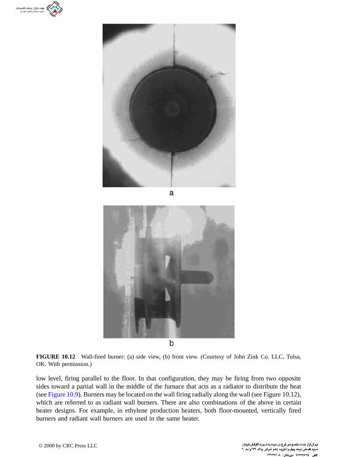
low level, firing parallel to the floor. In that configuration, they may be firing from two opposite sides toward a partial wall in the middle of the furnace that acts as a radiator to distribute the heat (see Figure 10.9). Burners may be located on the wall firing radially along the wall (see Figure 10.12), which are referred to as radiant wall burners. There are also combinations of the above in certain heater designs. For example, in ethylene production heaters, both floor-mounted, vertically fired burners and radiant wall burners are used in the same heater.
FIGURE 10.12 Wall-fired burner: (a) side view, (b) front view. (Courtesy of John Zink Co. LLC, Tulsa, OK. With permission.)
© 2000 by CRC Press LLC

Typical examples of process heaters are shown in Figure 10.13. Berman (1979) noted the following categories of process heaters: column reboilers, fractionating-column feed preheaters, reacter-feed preheaters including reformers, heat supplied to heat transfer media (e.g., a circulating fluid or molten salt), heat supplied to viscous fluids, and fired reactors including steam reformers and pyrolysis heaters.30 Six types of vertical-cylindrical fired heaters were given: all radiant, helical coil, crossflow with convection section, integral convection section, arbor or wicket type, and single-row/double-fired. Six basic designs were also given for horizontal-tube fired heaters: cabin, two-cell box, cabin with dividing bridgewall, end-fired box, end-fired box with side-mounted convection section, and horizontal-tube/single-row/double-fired. Many commonly used process heaters typi-cally have a radiant section and a convection section. Burners are fired in the radiant section to heat up tubes. Fluids flow through the tubes and are heated to the desired temperature for further processing. The fluids are preheated in the convection section and heated to the desired process temperature in the radiant section. Radiant heat transfer from the flames to the tubes is the most critical aspect of this heater because overheating of the tubes leads to tube failure and shutdown of the heater.31 The tubes may be horizontally or vertically oriented, depending on the particular heater design. Permissible average radiant flux rates range from 5000 to 18,000 Btu/hr-ft2 (16 to 57 kW/m2) of circumferential tube area, depending on the type of furnace.23
Feintuch and Negin (1996) discussed process heater design for delayed cokers.50 The traditional allowable average radiant flux rates range from 10,000 to 12,000 Btu/hr-ft2 (32 to 38 kW/m2). However, there has been a recent trend to reduce that to about 9000 Btu/hr-ft2 (28 kW/m2) to provide for longer run lengths, future capacity expansion, and a more conservative heater design. In delayed cokers, there is a gradual build-up of coke on the inside of the heater tubes that affects both the heat transfer to the oil in the tubes and the life of the tube. The coke build-up becomes a thermal resistance to heat flow. This reduces the heat transfer to the fluid in the tube, while simultaneously causing the tube wall to overheat because the heat cannot be dissipated as quickly as when there is no coke build-up.
A unique aspect of process heaters is that they are often natural draft. This means that no combustion air blower is used. The air is inspirated into the furnace by the suction created by the hot gases rising through the combustion chamber and exhausting to the atmosphere. Another unique aspect of these heaters is the wide range of fuels used, which are often by-products of the petroleum
FIGURE 10.13 Examples of process heaters. (Courtesy of CRC Press, Boca Raton, FL.32)
© 2000 by CRC Press LLC

refining process. These fuels may contain significant amounts of hydrogen, which has a large impact on the burner design. It is also fairly common for multiple fuel compositions to be used, depending on the operating conditions of the plant at any given time. In addition to hydrocarbons ranging up to C5, the gaseous fuels may also contain hydrogen and inerts (like CO2 or N2). The compositions can range from gases containing high levels of inerts to fuels containing high levels of H2. The flame characteristics for fuels with high levels of inerts are very different from fuels with high levels of H2. Figure 10.14 shows that the adiabatic flame temperature increases rapidly and non-linearly as the hydrogen content in CH4/H2 flames increases. The figure also shows that the adiabatic flame temperature decreases rapidly and nonlinearly as the nitrogen content in CH4/N2 flames increases. Add to that the requirement for turndown conditions, and the burner design becomes very challenging to maintain stability, low emissions, and the desired heat flux distribution over the range of conditions that are possible. Some plants use liquid fuels, like no. 2 to no. 6 fuel oil, sometimes by themselves and sometimes in combination with gaseous fuels. So-called combination burners use both a liquid and a gaseous fuel, which are normally injected separately through each burner.
Shires gave a general heat balance for a process heater:32
(10.3)
where •
Qf is the heat generated by combusting the fuel, •
Qg is the heat going to the load, •
Ql is the heat lost through the walls, and
•Qp is the heat carried out by the exhaust products. This is shown
schematically in Figure 10.15.The heat transfer from the hot combustion products to the tubes in the convection section is
forced convection flow over a bank of tubes. Colburn’s equation for this type of convection is:
(10.4)
FIGURE 10.14 Adiabatic equilibrium flame temperature for the stoichiometric combustion of ambient air with blends of H2 /CH4 and N2/CH4.
˙ ˙ ˙ ˙Q Q Q Qf g l p= + +
Nu f,d f= a Re Pr. .0 6 0 33
© 2000 by CRC Press LLC

where a = 0.33 for staggered tubes and 0.26 for in-line tubes, with the properties evaluated at the film temperature. A similar but more detailed correlation, is given by:33
(10.5)
where B and N are given in Table 10.1, F2 = 1, 0.97, 0.95, or 0.90 for 10, 8, 6, or 4 rows of tubes, respectively, and F1 is given by:
(10.6)
where Prw is the Prandtl number evaluated at the wall or tube surface temperature.
FIGURE 10.15 Process heater heat balance. (Courtesy of CRC Press, Boca Raton, FL.32)
TABLE 10.1Values of B and N
Range of Re
In-line Bank of Tubes Staggered Bank of Tubes
B N B N
10–300 0.742 0.431 1.309 0.360300–2 × 10⁵ 0.211 0.651 0.273 0.635
2 × 10⁵–2 × 10⁶ 0.116 0.700 0.124 0.700
Source: From J.W. Rose and J.R. Cooper, Technical Data on Fuel, 7th edition, British National Committee, London, 1977.
Nu f,d f= BFF N1 2
0 34Re Pr .
Fw
1
0 26
=⎛⎝⎜
⎞⎠⎟
Pr
Pr
.
f
© 2000 by CRC Press LLC

Berman (1979) gave equations and sample calculations for determining the heat transfer split between the radiant and convection sections.34 Graphs were provided for determining the average radiant heat transfer rate as functions of both the tube metal temperature and target wall (wall fired on in middle of heater to radiate to tubes) temperature for both vertical-cylindrical and horizontal-tube heaters. A graph was also provided for determining the maximum heat flux on a tube as a function of the tube geometry. Wimpress (1979) also gave a simplified method for calculating the performance of a fired heater.35
Talmor (1982) has written a book dealing with how to predict, control, and troubleshoot hot-spots in process heaters.36 The book gave a method for estimating the magnitude and location of the maximum combustion zone heat flux. It takes into account the firing rate of each burner, the number of burners, the flame length, the flame emissivity, the spacing between the burner and the tubes, the spacing between the burners, and the geometry of the firebox. The book included much empirical data specific to a variety of different process heaters and also gave many detailed examples that have been worked.
Figure 10.16 shows how the measured heat flux to the wall (normalized to the peak flux) of a furnace varied as a function of the vertical elevation and the firing rate for a fuel containing 78% natural gas and 22% H2. As expected, the heat flux increased with firing rate. The curves show the peak fluxes for a given firing rate were between about 10 and 20 ft (3 and 6 m). Figure 10.17 shows a similar graph where the fuel was 86% natural gas and 14% H2. The results are similar to the blend containing 22% H2. Figure 10.18 is a comparison of the measured heat fluxes for the two fuel blends at a fixed firing rate. The profiles are similar but the peaks occur at different vertical elevations.
10.4 HEAT TREATING
Heat treating involves the thermal treatment of metal to produce some type of enhanced performance characteristic. Typical material improvements include surface hardening, strengthening the part, relieving stresses, and improving ductility. Typical thermal treatments include annealing, brazing, carburizing, normalizing, sintering, and tempering. Annealing is a heat treatment used to remove internal stresses and to make a material less brittle by heating a part and then cooling it. This may be done under a protective atmosphere (commonly nitrogen) to prevent surface reactions if the
FIGURE 10.16 Heat flux profiles as a function of firing rate for a natural draft burner mounted in the floor of a furnace and firing vertically upward, using a fuel blend with 78% natural gas (Tulsa) and 22% H2 with 2% O2 in the exhaust gases.
© 2000 by CRC Press LLC

application is particularly sensitive or critical. Sometimes, a reducing agent like hydrogen may be added to the protective atmosphere to produce clean, bright surfaces. Brazing is a method of joining metals together using a non-ferrous filler material such as brass or a brazing alloy. The melting point of the braze material is lower than that of the metals being joined, which dictates the furnace temperature. Again, a protective atmosphere of nitrogen, possibly with small amounts of hydrogen or a hydrocarbon, may be used to produce high-quality parts. Dewpoint control in the atmosphere is often important in certain applications to minimize surface reactions with water at higher temperatures that would reduce the surface quality. Carburizing and neutral hardening refer to surface hardening of steels by adding carbon just to the surface of a part at a temperature high enough for the carbon to convert the surface from a lower carbon steel to a higher carbon steel. This must be done under an atmosphere, sometimes referred to as an endothermic gas, that containscarbon. The endothermic gas may have a composition of approximately 20% CO, 40% H2, and
FIGURE 10.17 Heat flux profiles as a function of firing rate for a natural draft burner mounted in the floor of a furnace and firing vertically upward, using a fuel blend with 86% natural gas (Tulsa) and 14% H2 with 2% O2 in the exhaust gases.
FIGURE 10.18 Heat flux profiles as a function of fuel blend for a natural draft burner mounted in the floor of a furnace and firing vertically upward at 6.5 × 10⁶ Btu/hr with 2% O2 in the exhaust gases.
© 2000 by CRC Press LLC
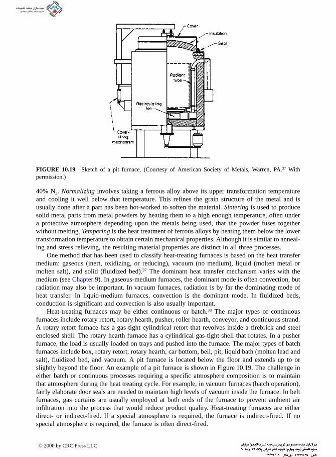
40% N2. Normalizing involves taking a ferrous alloy above its upper transformation temperature and cooling it well below that temperature. This refines the grain structure of the metal and is usually done after a part has been hot-worked to soften the material. Sintering is used to produce solid metal parts from metal powders by heating them to a high enough temperature, often under a protective atmosphere depending upon the metals being used, that the powder fuses together without melting. Tempering is the heat treatment of ferrous alloys by heating them below the lower transformation temperature to obtain certain mechanical properties. Although it is similar to anneal-ing and stress relieving, the resulting material properties are distinct in all three processes.
One method that has been used to classify heat-treating furnaces is based on the heat transfer medium: gaseous (inert, oxidizing, or reducing), vacuum (no medium), liquid (molten metal or molten salt), and solid (fluidized bed).37 The dominant heat transfer mechanism varies with the medium (see Chapter 9). In gaseous-medium furnaces, the dominant mode is often convection, but radiation may also be important. In vacuum furnaces, radiation is by far the dominating mode of heat transfer. In liquid-medium furnaces, convection is the dominant mode. In fluidized beds, conduction is significant and convection is also usually important.
Heat-treating furnaces may be either continuous or batch.38 The major types of continuous furnaces include rotary retort, rotary hearth, pusher, roller hearth, conveyor, and continuous strand. A rotary retort furnace has a gas-tight cylindrical retort that revolves inside a firebrick and steel enclosed shell. The rotary hearth furnace has a cylindrical gas-tight shell that rotates. In a pusher furnace, the load is usually loaded on trays and pushed into the furnace. The major types of batch furnaces include box, rotary retort, rotary hearth, car bottom, bell, pit, liquid bath (molten lead and salt), fluidized bed, and vacuum. A pit furnace is located below the floor and extends up to or slightly beyond the floor. An example of a pit furnace is shown in Figure 10.19. The challenge in either batch or continuous processes requiring a specific atmosphere composition is to maintain that atmosphere during the heat treating cycle. For example, in vacuum furnaces (batch operation), fairly elaborate door seals are needed to maintain high levels of vacuum inside the furnace. In belt furnaces, gas curtains are usually employed at both ends of the furnace to prevent ambient air infiltration into the process that would reduce product quality. Heat-treating furnaces are either direct- or indirect-fired. If a special atmosphere is required, the furnace is indirect-fired. If no special atmosphere is required, the furnace is often direct-fired.
FIGURE 10.19 Sketch of a pit furnace. (Courtesy of American Society of Metals, Warren, PA.37 With permission.)
© 2000 by CRC Press LLC

Orzechowski and Hughes (1999) showed how the importance of forced convection and thermal radiation vary as a function of the furnace temperature in heat treating applications.39 Forced convection heating is recommended for furnace temperatures below 1000°F (540°C). Radiation heating is recommended for furnace temperatures above 1000°F (540°C).
10.4.1 STANDARD ATMOSPHERE
There are some heat-treating processes that do not require a special atmosphere, where the gas around the parts being treated is air and the products of combustion. One example is a car bottom furnace, which is often used to relieve stresses in large welded parts. Furnaces used for annealing also do not usually require any specific gas composition around the parts being treated. Another example is a rotary hearth, continuous heat treating furnace, shown in Figure 10.20, which operates like a revolving door with parts entering on one part of the circle and exiting at another part after rotating some angular distance. Rotary hearth furnaces are often used for heating larger workpieces.
Ferguson (1979) compared the energy requirements for indirect-fired (radiant tube) and direct-fired (with recuperation) furnaces for batch annealing furnaces.40 The direct-fired furnace used about a third less energy than the indirect-fired furnace. In the radiant tube furnace, over half of the energy is lost in the flue gases, compared to only 30% for the direct-fired recuperative furnace. This shows the importance of the heating method on energy consumption. The analysis assumed that no special atmosphere was required for the heating application.
10.4.2 SPECIAL ATMOSPHERE
In this type of process, the combustion products cannot come in contact with the metal load, as they would reduce the product quality. There are two basic types of special atmospheres that are commonly used, depending on the type of heat treating process. In the first type of special atmosphere, the objective is to prevent certain chemicals from reaching the part that could contam-inate the surface. One such type is sometimes referred to as a neutral atmosphere, where for example, an inert gas like helium is used to protect metal products from oxidation, which causes scale formation on the metal surface that reduces the metal yield and product quality. Another type of protective atmosphere is the absence of any gases, created by a vacuum, contacting the part surface. Some specific contaminants that can detrimentally affect a part’s surface quality include oxygen (air), water, carbon-containing materials, hydrogen, and nitrogen. Oxygen and water can cause surface oxidation, carbon-containing materials can cause surface hardening, hydrogen can cause
FIGURE 10.20 Sketch of a rotary hearth furnace. (Courtesy of American Society of Metals, Warren, PA.37
With permission.)
© 2000 by CRC Press LLC

TABLE 10.2
embrittlement, and nitrogen can cause nitriding. The latter two are sometimes desirable, but they can also be detrimental, depending on the desired part characteristics.
The second type of special atmosphere is where a specific reaction is desired by the atmosphere contacting the part surface at an elevated temperature. One example is a carburizing atmosphere that contains a specific amount of gases containing carbon, which diffuses into the metal surface for hardening. This is used, for example, in tool steels that require hard outer surfaces. An atmosphere containing nitrogen can be used to nitride a metal. Table 10.2 shows common special furnace atmosphere compositions and their applications.41 Many of these atmospheres are directly or indi-rectly produced by combusting hydrocarbon fuels. One example of a furnace that has a protective atmosphere is a bell furnace. The inner part of the furnace has a heated muffle that contains a protective atmosphere — often hydrogen or hydrogen blends. These furnaces are commonly used for annealing steel coils. Another example of a furnace using a protective atmosphere is a roller hearth, as shown in Figure 10.21. The photograph shows an entrance vestibule that helps contain the protective atmosphere. Furnace pressure control is especially important in furnaces containing special atmospheres, not only to ensure that ambient air does not leak into the furnace but also that not much special atmosphere leaks out of the furnace, which would be wasted cost.42
Thekdi et al. (1985) described an indirect, natural gas-fired heating system used where con-trolled atmospheres are needed for heat treating.43 The heat source was a high-intensity radiant tube burner capable of temperatures greater than 2000°F (1100°C). Heat flux improvements of up to three times conventional heating systems were measured. Peak fluxes up to 21,900 Btu/hr-ft2
(69 kW/m2) were measured which compared to fluxes from conventional systems of 7930 Btu/hr-ft2 (25 kW/m2). As shown in Figure 10.22, the heat flux varied along the length of the tube.
Liang et al. (1987) discussed the application of ceramic tube burners in indirect-fired heat-treating furnaces.44 They described developments of advanced materials to increase the maximum operating temperatures of metallic radiant tubes that were limited to 1800°F (1000°C). Furnaces operating at higher temperatures typically used electric heating, which is often more expensive than using natural gas. Advanced ceramic radiant tube burners need to be capable of radiant outputs of at least 95 kW/m2 (30,000 Btu/hr-ft2).
Special Atmosphere Compositions and Applications
Nominal Composition (% by volume)
Class Description N2 CO CO2 H2 CH4 Application
101 Lean exothermic 86.8 1.5 10.5 1.2 0 Oxide coating of steel102 Rich exothermic 71.5 10.5 5.0 12.5 0.5 Bright annealing; copper brazing;
sintering201 Lean prepared nitrogen 97.1 1.7 0 1.2 0 Neutral heating202 Rich prepared nitrogen 75.3 11.0 0 13.2 0.5 Annealing and brazing of stainless
steels301 Lean endothermic 45.1 19.6 0.4 34.6 0.3 Clean hardening302 Rich endothermic 39.8 20.7 0 38.7 0.8 Carburizing (enriched 301)402 Charcoal 64.1 34.7 0 1.2 0 Carburizing501 Lean exothermic-endothermic 63.0 17.0 0 20.0 0 Clean hardening502 Rich exothermic-endothermic 60.0 19.0 0 21.0 0 Carburizing601 Dissociated ammonia 25.0 0 0 75.0 0 Brazing; sintering621 Lean combusted ammonia 99.0 0 0 1.0 0 Neutral heating622 Rich combusted ammonia 80.0 0 0 20.0 0 Sintering of stainless powders
Source: From ASM Committee on Furnace Atmospheres, Metals Handbook, 8th edition, Vol. 2, American Society for Metals, Metals Park, OH, 1964, 67-84.
© 2000 by CRC Press LLC
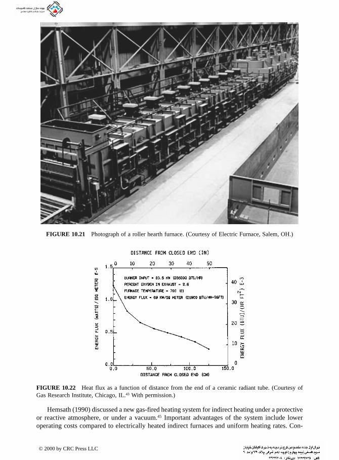
Hemsath (1990) discussed a new gas-fired heating system for indirect heating under a protective or reactive atmosphere, or under a vacuum.45 Important advantages of the system include lower operating costs compared to electrically heated indirect furnaces and uniform heating rates. Con-
FIGURE 10.21 Photograph of a roller hearth furnace. (Courtesy of Electric Furnace, Salem, OH.)
FIGURE 10.22 Heat flux as a function of distance from the end of a ceramic radiant tube. (Courtesy of Gas Research Institute, Chicago, IL.43 With permission.)
© 2000 by CRC Press LLC

ventional gas-fired indirect furnaces use radiant tubes. The system described by Hemsath used forced convection to heat the vacuum vessel, as shown in Figure 10.23. The impinging jets consist of the exhaust products from a single burner as noted in the schematic of the furnace shown in Figure 10.24. The maximum reported temperature for a pilot-scale furnace was 1250°F (677°C), which was expected to be raised to 1750°F (954°C) by subsequent development. The application of this novel furnace design was discussed for batch coil annealing and as a thermal cleaner for aluminum borings and scrap.
Copes and Brooks (1991) tested a ceramic composite material called Siconex™ for use in a controlled-atmosphere furnace.46 The material, which is a fiber-reinforced composite, was tested in endothermic, exothermic, and nitrogen-based atmospheres. Tubular shapes were tested with and without coatings (23 different coatings were tested) to determine their properties under the different atmospheres. The performance tests for the coatings included burst strength, permeability, adhesion, stability, cracking, and maintenance of emissivity. Only two of the coatings performed well over
FIGURE 10.23 Convection heating of an indirect-fired furnace. (Courtesy of ASME, New York.45 With permission.)
FIGURE 10.24 Schematic of an indirect-fired furnace. (Courtesy of ASME, New York.45 With permission.)
© 2000 by CRC Press LLC

a wide range of conditions. The inert atmosphere proved to be the most detrimental to the strength of the ceramic samples.
Schultz et al. (1992) studied heat transfer in a gas-fired, high-temperature “soft” vacuum (1 to
100 torr) furnace with a design operating temperature of 2350°F (1290°C).47 The furnace was designed for hardening tool steels, annealing stainless steel, and for sintering and brazing applica-tions. The furnace was heated with single-ended radiant tube burners. The object of the study was to model the heat transfer in the furnace with various silicon carbide radiant tube sizes ranging from 3.25 to 6 in. (8.26 to 15 mm) o.d., quantities, and locations. The following parameters were used in the evaluation: empty furnace temperature uniformity, surface temperature uniformity during heating, process or cycle time, and temperature uniformity within the load. A combination of modeling and experiments showed that for the given furnace configuration, four 6-in. (15 mm) o.d. single-ended radiant tubes provided the most optimized results.
Erinov et al. (1996) described the development of a low-inertia, high-efficiency heat-treating furnace using indirect heating with contained, flat, gas-fired IR burners.48 The claimed benefits included fast heat-up and cool-down, better heating uniformity, higher thermal efficiency, increased productivity, and low NOx emissions. The burner design incorporated flue gas heat recuperation and had high surface temperature uniformity.
Kurek et al. (1998) presented the development of high-temperature uniformity, natural gas-fired, flat radiant panels for use in indirect-fired heat treating furnaces.49 These panels were designed as a potential replacement for radiant tube burners. They had increased radiating surface area, which means they could be operated at lower temperatures to achieve the same heat flux output. The lower radiating temperature and high surface area improved the temperature uniformity to the load, which improved product quality. Because of the higher surface area, less refractory was required in the furnace, which meant faster heat-up and cool-down. Self-heat recuperation increased the thermal efficiency to over 70%. The radiant output was approximately 120 kW/m2 (38,000 Btu/hr-ft2).
REFERENCES
1. D. Traub, Indirect vs. direct: the heat transfer method does affect the process, Process Heating, 6(2), 26-29, 1999.
2. Anonymous, Ceramic tile burner improves performance of infrared predryer, Process Heating, 4(7), 43-45, 1997.
3. P. Mattsson, J. Perkonen, and A. Riikonen, Infrared drying of coated paper, Proc. 1989 International Gas Research Conf., T.L. Cramer, Ed., Govt. Institutes, Rockville, MD, 1989, 1308-1316.
4. M. Pettersson and S. Stenström, Evaluation of gas-fired and electrically heated industrial infrared paper dryers, Proc. 1998 International Gas Research Conf., Vol. V: Industrial Utilization and Power Generation, D. Dolenc, Ed., Govt. Institutes, Rockville, MD, 1998, 100-112.
5. J. Riikonen, E. Härkönen, and S. Palosaari, Modeling of infrared drying of pulp, in Drying ‘87, A.S. Majumdar, Ed., Hemisphere, Washington, D.C., 1987, 18-23.
6. A. Williams-Gardner, Industrial Drying, Leonard Hill, London, 1971.7. R.B. Keey, Dryers, in International Encyclopedia of Heat & Mass Transfer, G.F. Hewitt, G.L. Shires,
and Y.V. Polezhaev, Eds., CRC Press, Boca Raton, FL, 1997, 337-342.8. C.E. Sloan, Drying systems and equipment, Chem. Eng., 74(14), 169-200, 1967.
8a. B.J. Ezerski and G.P. Megan, Boosting the performance of your convection oven, Process Heating,7(1), 22–26, 2000.
8b. J.R. Cornforth, Ed., Combustion Engineering and Gas Utilisation, E&FN Spon, London, 1992.9. T. Berntsson, P.-A. Franck, and A. Åsblad, Learning from Experiences with Process Heating in the
Low and Medium Temperature Ranges, CADDET Energy Efficiency, Sittard, The Netherlands, 1997.10. C.E. Bean and J.M. Cocagne, Assessment of Gas-Fired Infrared Heaters in the Paper Industry, Gas
Research Institute Report GRI-96/0087, Chicago, IL, 1996.11. M.N.A. Hawlader, S.K. Chou, and K.J. Chua, Development of design charts for tunnel dryers, Int. J.
Energy Research, 21(11), 1023-1037, 1997.
© 2000 by CRC Press LLC
12. A. Garg, Optimize fired heater operations to save money, Hydrocarbon Processing, 76(6), 97-104, 1997.
13. W.L. Nelson, Petroleum Refinery Engineering, second edition, McGraw-Hill, New York, 1941.14. G.R. Martin, Heat-flux imbalances in fired heaters cause operating problems, Hydrocarbon Processing,
77(5), 103-109, 1998.15. R. Nogay and A. Prasad, Better design method for fired heaters, Hydrocarbon Processing, 64(11),
91-95, 1985.16. A. Garg, Revamp fired heaters to increase capacity, Hydrocarbon Processing, 77(6), 67-80, 1998.17. H.C. Hottel, First estimates of industrial furnace performance — The one-gas-zone model reexamined,
in Heat Transfer in Flames, N.H. Afgan and J.M. Beer, Eds., Scripta Book Co., Washington, D.C., 1974, 5-28.
18. H. Futami, R. Hashimoto, and H. Uchida, Development of new catalyst and heat-transfer design method for steam reformer, J. Fuel Soc. Japan, 68(743), 236-243, 1989.
19. H. Gunardson, Industrial Gases in Petrochemical Processing, Marcel Dekker, New York, 1998.20. J.D. Fleshman, FW hydrogen production, in Handbook of Petroleum Refining Processes, 2nd edition,
R.A. Myers, Ed., McGraw-Hill, New York, 1996, chap. 6.2.21. K. Kudo, H. Taniguchi, and K. Guo, Heat-transfer simulation in a furnace for steam reformer, Heat
Transfer — Japanese Research, 20(8), 750-764, 1992.22. H.S. Kurek, M. Khinkis, W. Kunc, A. Touzet, A. de La Faire, T. Landais, A. Yerinov, and O. Semernin,
Flat radiant panels for improving temperature uniformity and product quality in indirect-fired furnaces, Proc. 1998 International Gas Research Conf., Vol. V: Industrial Utilization and Power Generation, D. Dolenc, Ed., Gas Research Institute, Chicago, 1998, 100-112.
23. D.Q. Kern, Process Heat Transfer, McGraw-Hill, New York, 1950.24. N.P. Lieberman, Troubleshooting Process Operations, PennWell Books, Tulsa, OK, 1991.25. H.S. Bell and L. Lowy, Equipment, in Petroleum Processing Handbook, W.F. Bland and R.L. Davidson,
Eds., McGraw-Hill, New York, 1967, chap. 4.25a. A. Garg, Trimming NOx from furnaces, Chem. Eng., 99(11), 122–124, 1992.25b. A. Garg and H. Ghosh, Good heater specifications pay off, Chem. Eng., 95(10), 77–80, 1988.25c. A. Garg, How to boost the performance of fired heaters, Chem. Eng., 96(11), 239–244, 1989.25d. A. Garg, Better burner specifications, Hydrocarbon Processing, 68(8), 71–72, 1989.26. C.J. Hoogendoorn, C.M. Ballintijn, and W.R. Dorresteijn, Heat-flux studies in vertical tube furnaces,
J. Inst. Fuel, 43, 511-516, 1970.27. N. Selçuk, R.G. Siddall, and J.M. Beér, Prediction of the effect of flame length on temperature and
radiative heat flux distributions in a process fluid heater, J. Inst. Fuel, 48, 89-96, 1975.28. H.L. Berman, Fired heaters. II. Construction materials, mechanical features, performance monitoring,
in Process Heat Exchange, V. Cavaseno, Ed., McGraw-Hill, New York, 1979, 293-302.29. A.J. Johnson and G.H. Auth, Fuels and Combustion Handbook, first edition, McGraw-Hill, New York,
1951.30. H.L. Berman, Fired heaters. I. Finding the basic design for your application, in Process Heat Exchange,
V. Cavaseno, Ed., McGraw-Hill, New York, 1979, 287-292.31. V. Ganapathy, Applied Heat Transfer, PennWell Books, Tulsa, OK, 1982.32. G.L. Shires, Furnaces, in The International Encyclopedia of Heat & Mass Transfer, G.F. Hewitt, G.L.
Shires, and Y.V. Polezhaev, Eds., CRC Press, Boca Raton, FL, 1997, 493-497.33. J.W. Rose and J.R. Cooper, Technical Data on Fuel, 7th edition, British National Committee, London,
1977.34. H.L. Berman, Fired heaters. III. How combustion conditions influence design and operation, in Process
Heat Exchange, V. Cavaseno, Ed., McGraw-Hill, New York, 1979, 303-314.35. N. Wimpress, Generalized method predicts fired-heater performance, in Process Heat Exchange, V.
Cavaseno, Ed., McGraw-Hill, New York, 1979, 320-327.36. E. Talmor, Combustion Hot Spot Analysis for Fired Process Heaters, Gulf Publishing, Houston, 1982.37. H.E. Boyer, Practical Heat Treating, American Society for Metals, Metals Park, OH, 1984.38. ASM Committee on Gas Carburizing, Case Hardening of Steel, in Metals Handbook, 8th edition,
Vol. 2: Heat Treating, Cleaning and Finishing, Amer. Soc. For Metals, Metals Park, Ohio, 1964, 93-114.39. N.J. Orzechowski and D.L. Hughes, Selecting the proper furnace for vacuum tempering applications,
Industrial Heating, LXVI(9), 45-49, 1999.
© 2000 by CRC Press LLC

40. N.T. Ferguson, Energy and furnace design for batch annealing and heat treating furnaces, Iron & Steel Engineer, 56(6), 31-33, 1979.
41. ASM Committee on Furnace Atmospheres, Furnace atmospheres and carbon control, in Metals
Handbook, 8th edition, Vol. 2: Heat Treating, Cleaning and Finishing, American Society for Metals, Metals Park, OH, 1964, 67-84.
42. W. Trinks and M.H. Mawhinney, Industrial Combustion, Vol. II, 4th edition, Wiley, New York, 1967.43. A.C. Thekdi, S.R. Huebner, and M.A. Lukasiewicz, Development of an indirect gas-fired high tem-
perature heating system, Proc. 1984 International Gas Research Conf., Govt. Institutes, Rockville, MD, 1985, 709-718.
44. W.W. Liang, M.E. Schreiner, S.J. Sikirica and E.S. Tabb, Application of ceramic tubes in high temperature furnaces, Proc. 1986 International Gas Research Conf., T.L. Cramer, Ed., Govt. Institutes, Rockville, MD, 1987, 875-888.
45. K.H. Hemsath, A novel gas fired heating system for indirect heating, in Fossil Fuel Combustion Symposium 1990, S.N. Singh, Ed., New York, ASME PD-Vol. 30, 155-159, 1990.
46. J.S. Copes and D.L. Brooks, Siconex™ coupon testing in controlled-atmosphere furnaces, in Fossil Fuel Combustion — 1991, R. Ruiz, Ed., New York, ASME PD-Vol. 33, 155-160, 1991.
47. T.J. Schultz, R.A. Schmall, and I. Chan, Selection of a heating system for a high temperature gas fired soft vaccum furnace, in Fossil Fuels Combustion — 1992, R. Ruiz, Ed., New York, ASME PD-Vol. 39, 23-30, 1992.
48. A.E. Erinov, A.M. Semernin, V.A. Povarenkov, M.J. Khinkis, and H.A. Abbasi, Development of a gas-fired, low-inertia, high-efficiency heat treating furnace, Proc. of 1995 International Gas Research Conf., D.A. Dolenc, Ed., Govt. Institutes, Rockville, MD, 1986, 2774-2773.
49. H.S. Kurek, M. Khinkis, W. Kunc, A. Touzet, A. de La Faire, T. Landais, A. Yerinov, and O. Semernin, Flat radiant panels for improving temperature uniformity and product quality in indirect-fired furnaces, Proc. 1998 International Gas Research Conf., Vol. V: Industrial Utilization and Power Generation, D. Dolenc, Ed., Govt. Institutes, Rockville, MD, 1998, 100-112.
50. H.M. Feintuch and K.M. Negin, FW Delayed-Coking Process, in Handbook of Petroleum Refining Processes, 2nd edition, R.A. Meyers, Ed., McGraw-Hill, New York, 1996, chap. 12.2.
© 2000 by CRC Press LLC

11 Higher Temperature Applications
11.1 INTRODUCTION
The designation “higher temperature application” is somewhat relative, but here it refers to processeswith furnace temperatures above about 2200°F (1200°C). The major applications considered in thischapter include furnaces and combustors used in the metals, minerals, and waste incinerationindustries. In general, the dominant heat transfer mechanism in those industries is thermal radiation.This is in contrast to lower temperature applications where both radiation and forced convectionare often important.
11.1.1 FURNACES
A furnace is a device where heat is transferred to a material to effect physical or chemical changesin the material.1 For the purposes of this book, the energy is generated by the combustion of afossil fuel inside the furnace. Industrial furnaces are refractory-lined vessels designed both to keepenergy inside to minimize heat losses and to radiate energy to the load. The heat transfer mechanismsthat are important in furnaces are discussed in Chapter 9.
11.1.2 INDUSTRIES
The three primary higher temperature industries considered in this chapter include the metals,minerals, and waste incineration industries. Each of these requires higher temperatures to eithermelt high-melting-point materials or destroy waste materials processed in their furnaces. Each ofthese industries has slightly different requirements and operating conditions compared to the othersthat makes the heat transfer analysis slightly different in each case.
In the metals industries, there are generally two types of high temperature processes: metalproduction and parts production from that metal. Metal heat treatment was considered in Chapter 10and is not included here as it generally is done at lower temperatures. Final finished parts are notusually made directly in a single process starting with raw materials. In the case of metals produc-tion, many of these processes are batch in nature. Solid raw ore materials or scrap metals are heatedand melted to the liquid state. The molten metal is then blended with the appropriate ingredientsto get the desired grade of metal. Chemical reactions may occur in the molten metal. In the secondtype of high temperature metal heating process, a specific grade of metal is melted and then formedinto a specific shape or part. For example, a given grade of steel may be cast into sheet, plate, I-beams, bar stock, or other shapes. Another example would be taking a specific grade of aluminumand casting it to make a part like an engine component. The batch nature of many high temperaturemetals processes complicates the heat transfer analysis because of the transient nature and the hightemperature gradients and nonuniformity caused by the discontinuous processing.
In the minerals industries, solids are often blended together in specific ratios and then processedin a high-temperature furnace in a continuous process and then made directly into the final finishedpart. Unlike most metals processes, the mineral products go from raw materials to the final finishedpart in a single process. For example, in glass manufacturing, scrap glass, sand, and many other
© 2000 by CRC Press LLC

components are preblended and fed into a continuous furnace where they are made into moltenglass, which is then fed directly into a casting process to make finished glass parts like windowsor car windshields. There are often chemical reactions occurring during the heating and meltingportion of the cycle. The continuous nature of high temperature minerals processing simplifies theheat transfer analysis because of the steady-state operating conditions.
The waste incineration industry is somewhat unique in that the desired result is usually not anend product but the destruction of contaminants rather than the production of a new material. Insome cases, the end product may be a cleaned solid material such as in soil decontamination, forexample, resulting from the destruction of the contaminants. Waste incineration processes areusually continuous, which makes heat transfer analysis a little simpler, but mass transfer is oftenimportant as liquid and solid waste materials are vaporized and combusted. If the contaminantscontain significant quantities of hydrocarbons, these may also be used as heat sources in additionto the fuel supplied through the burners. Also, enough air must be supplied to burn both the fueland the hydrocarbons to ensure complete destruction of the contaminants (see section 4.1.1.2).
11.2 METALS INDUSTRY
The heating and melting of metal has been around for centuries. Many of the techniques still beingused today were developed years ago and are often little-changed. As is customary, the metalsindustry has been broken into two categories: ferrous and non-ferrous. The ferrous industry includesiron- and steelmaking. The non-ferrous industry includes essentially all other metals, but the morecommon ones include aluminum, brass, copper, and lead.
11.2.1 FERROUS METAL PRODUCTION
There are many processes in the iron and steel industries that use large quantities of fossil fuelenergy. Examples include the blast furnace, the open hearth furnace, and the basic oxygen furnace(BOF). However, these processes do not use burners. The combustion occurs inside the vessels inconjunction with processing the materials inside. Therefore, these processes are not consideredhere as they are not industrial combustion processes in the sense of the definition used in this book.Although a furnace like the electric arc furnace, which is discussed next, uses electricity as theprimary energy source, it also often uses supplemental burners and is therefore considered here.Lehrman et al. (1998) have listed the following applications in steel mills that use gaseous fuels:coke-oven heating, blast-furnace stoves, gas turbines for power generation, boilers, soaking pits,reheating furnaces, forge and blacksmith furnaces, normalizing and annealing furnaces, controlled-cooling pits, foundry core ovens, blast furnace and steel ladle drying, drying of blast-furnacerunners, hot-top drying, ladle preheating, and oxy/fuel burners.2 Several of those that are “conven-tional” combustion applications as defined here are considered next. A relatively recent batchsteelmaking process, known as the energy optimizing furnace (EOF), uses oxy/fuel burners to assistin melting a blend of approximately 50% scrap and 50% hot metal.3 However, since the EOF isprimarily used only in Brazil, it is not included here.
11.2.1.1 Electric Arc Furnace
Even before the arrival of the BOF, a major alternative to conventional ore-based steelmaking hadbegun to gain acceptance.4 The electric arc furnace (EAF) was conceived as a unit to melt scrapsteel and recycle the iron units back to useful service. It did not rely on molten iron from a blastfurnace, but rather solid scrap was melted by energy input from electrical arcs passed betweenthree carbon electrodes. Originally, this furnace was conceived as an all-electric melter. Freedomfrom the blast furnace and comparatively cheap electric power fueled the growth of the EAF,particularly in what came to be known as mini-mills.
© 2000 by CRC Press LLC

Due to the very high temperature requirements in most ferrous metal processes, oxy/fuel burners(see Chapter 12) have become standard equipment on most EAFs.5 Initially, firing through the slagdoor, oxy/fuel burners mounted on a boom or a carriage were introduced to increase scrap melting.Later, to efficiently target the coldspots in the EAF, the burner location was moved to either theroof or sidewalls, to aim at the coldspots associated with the spaces between the electrodes, withone to four burners in a furnace providing supplemental energy. Figure 11.1 shows a sketch of athree-burner, wall-fired supplemental system firing between the electrodes. In addition to produc-tivity improvements of 5% to 20%, the burners provide economical energy for melting scrap atlower cost.
Heat transfer from the oxy/fuel burners to the scrap metal occurs by forced convection fromthe combustion products to the scrap and by radiation from the flame to the scrap.6 Since the heattransfer is dependent on the temperature difference between the scrap and the heat source (com-bustion gases and flame), the oxy/fuel burners are most effective immediately after new cold scraphas been added to the EAF. The burners are often discontinued after half of the meltdown periodis complete in order to get reasonable efficiencies.7 There is also thermal conduction betweencontacting pieces of scrap and from the heated iron oxide (scale) layer on the outside of the scrapto the scrap metal under the scale layer. This mode of heat transfer is obviously undesirable becausethe oxidation layer on the scrap reduces the product quality and the yield and is therefore itselfundesirable. The reported overall heat transfer efficiencies for the oxy/fuel scrap heating rangefrom 50% to 75%.8 Figure 11.2 shows how the efficiency decreases with the time into the melt-down.9 By 50% into the meltdown, the instantaneous efficiency is below 40%. This is a result ofthe reduction in heat transfer as the scrap temperature increases.
Oxy/fuel burners are most efficient during cold scrap heating and meltdown. Typically, burnereffectiveness decreases during the latter half of the meltdown period from an initial 60%–80% toless than 20% when firing on a flat molten bath. Excessive use of burners with low efficiency canresult in yield loss and potential furnace damage due to higher offgas temperatures.
With regard to design considerations, it is important to maximize flame velocity for maximumheat transfer efficiency (i.e., deeper scrap penetration and higher convective heat flux). By usingthe smaller diameter burners for the available oxygen and fuel supply pressures and desired firingrate, the highest flame velocity is achieved. Converging/diverging nozzle designs have also beensuccessfully used in a number of burner designs.
An efficient oxy/fuel practice typically supplies 25% of the total energy required to melt thesteel. This may be higher or lower, depending on the desired results and characteristics of thefurnace and operation in question. The optimum burner firing rate is limited by how quickly the
FIGURE 11.1 Electric arc furnace (EAF) with three supplemental burners mounted in the sidewalls andfiring between the three electrodes. (Courtesy of Air Products, Allentown, PA. With permission.)
© 2000 by CRC Press LLC

scrap can absorb the heat supplied by the burners. In other words, the optimum firing rate is at thepoint where the heat transfer efficiency to the scrap is at a maximum (see Figure 11.3). Experienceand energy balance-based computer models are often used as aids in predicting the optimum firingrate. In practice, the firing rate is further optimized during burner start-up by experimenting withdifferent firing rates while monitoring melting rate, yield, and offgas temperatures.
Burners must have the flexibility of operating in either the fuel-rich or fuel-lean mode. Theycan be fired fuel-rich with a bushy, luminous flame early in the heat to preheat scrap withoutexcessive bridging or welding of the scrap, and then switched to an oxygen-rich mode to cut awayscrap and assist with uniform melt-in. Operating in an oxygen-rich mode is beneficial for slag doorinstallations to assist with cutting away the scrap to allow earlier use of an oxygen/carbon lancemanipulator to produce a foamy slag.
Battles and Knowles (1985) reported the use of oxy/gas burners to improve the productivity inelectric arc furnaces by supplemental heating.10 A schematic of the wall-mounted burner systemis shown in Figure 11.4. A water-cooled, oxy/gas burner was chosen to accelerate the melting rate
FIGURE 11.2 Oxy/fuel burner efficiency vs. time into meltdown for an electric arc furnace. (Courtesy ofAISE Steel Foundation, Pittsburgh, PA.5 With permission.)
FIGURE 11.3 Optimum firing rate is at maximum heat transfer efficiency. (Courtesy of CRC Press, BocaRaton, FL.4)
© 2000 by CRC Press LLC

in the colder areas of the furnace. On a 100-ton EAF, melting times were reduced by 20% to 35%and overall fuel consumption (electricity and natural gas) decreased by 10%. Another importantbenefit included reduced consumption of refractory and electrodes.
Sikirica (1987) described field test results for the use of oxy/gas burners in smaller EAFs(<30 tons) often used in foundries.11 Conventional oxy/gas burners can potentially damage smallerEAFs because the flame lengths would impinge on the furnace walls. Normally, the oxy/gas burnerswould be fired simultaneously with the arcing electrodes. For the smaller EAFs, the process wasmodified so that the oxy/gas burners fired before using the electrodes, to minimize the possibilityof flame impingement. The burners preheated the scrap metal in the colder parts of the furnace.Results showed a reduction in melting time ranging from 16% to 20% compared to all-electricmelting.
11.2.1.2 Smelting
Smelting is a bulk production process where solid metal ore mixtures are heated which causes achemical change that results in liquid metal. This process is done in a furnace often referred to asa smelter. The liquid phase may be either a liquid metal sulphide (matte) common in the productionof copper and nickel, or a metallic phase common for the production of iron, steel, lead, zinc, andaluminum. The two most common smelting processes are flash smelting and bath smelting. Depend-ing on the specific production method, large quantities of heat are normally required to melt themetal ore, which is where heat transfer from a combustion process is important.
Davila et al. (1995) described an oxy/fuel rotary furnace process for smelting white cast-ironand low alloy cast-carbon steels.12 The main parameters studied were the furnace lining, raw materialcomposition, load protection (slag), flame types and temperature, and furnace rotation speed. Themain measurements included the chemical analysis of each heat, analysis of the gas content, heatperformance, metal yield, and slag analysis. The flames were only slightly oxidizing to minimizemetal oxidation, which would reduce yields. This process reduced energy consumption by morethan 35% compared to electric induction melting.
11.2.1.3 Ladle Preheating
Another major use of burners in the steel industry’s melt shops is for ladle preheating, as shownin Figure 9.16. Figure 11.513 shows a ladle that is used to transport molten metal in steel mills fromthe melting furnace to the casting station. Ladles are refractory-lined cylindrical vessels closed
FIGURE 11.4 Gas-fired burners for supplemental heating in an electric arc furnace. (Courtesy of Govern-ment Institutes, Rockville, MD.10 With permission.)
© 2000 by CRC Press LLC
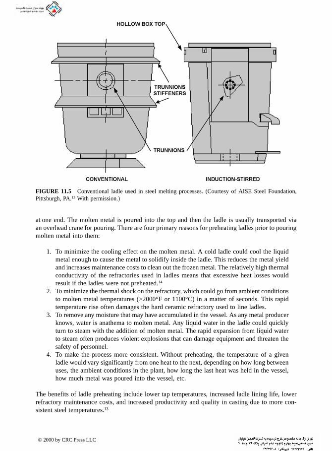
at one end. The molten metal is poured into the top and then the ladle is usually transported viaan overhead crane for pouring. There are four primary reasons for preheating ladles prior to pouringmolten metal into them:
1. To minimize the cooling effect on the molten metal. A cold ladle could cool the liquidmetal enough to cause the metal to solidify inside the ladle. This reduces the metal yieldand increases maintenance costs to clean out the frozen metal. The relatively high thermalconductivity of the refractories used in ladles means that excessive heat losses wouldresult if the ladles were not preheated.14
2. To minimize the thermal shock on the refractory, which could go from ambient conditionsto molten metal temperatures (>2000°F or 1100°C) in a matter of seconds. This rapidtemperature rise often damages the hard ceramic refractory used to line ladles.
3. To remove any moisture that may have accumulated in the vessel. As any metal producerknows, water is anathema to molten metal. Any liquid water in the ladle could quicklyturn to steam with the addition of molten metal. The rapid expansion from liquid waterto steam often produces violent explosions that can damage equipment and threaten thesafety of personnel.
4. To make the process more consistent. Without preheating, the temperature of a givenladle would vary significantly from one heat to the next, depending on how long betweenuses, the ambient conditions in the plant, how long the last heat was held in the vessel,how much metal was poured into the vessel, etc.
The benefits of ladle preheating include lower tap temperatures, increased ladle lining life, lowerrefractory maintenance costs, and increased productivity and quality in casting due to more con-sistent steel temperatures.13
FIGURE 11.5 Conventional ladle used in steel melting processes. (Courtesy of AISE Steel Foundation,Pittsburgh, PA.13 With permission.)
© 2000 by CRC Press LLC

Today’s refractories and steelmaking processes often require ladle preheat temperatures above2000°F (1100°C), which can be difficult to obtain with the relatively low temperatures generatedby conventional air/fuel flames. Because of their higher flame temperature, oxy/fuel burners providethe energy required for ladle preheating to reach the desired temperature in a shorter period of timewith minimum flue losses and maximum fuel efficiency (see Chapter 12). Even with high-temper-ature flames, Tomazin et al. (1986) showed that although the inside ladle refractory temperature(hot face) of an initially cold dry ladle heats up to 2000°F (1100°C) in about 8 hours, the outsideladle refractory temperature next to the steel shell (cold face) only heats up to about 300°F (150°C).15
Steady-state may not be reached in the ladle refractory until 18 hours after the start of the heatingcycle. Heating the refractory too quickly should be avoided because of the nonequilibrium temper-ature profile in the refractory, excessive stresses on the shell, and excessive shock on the refractorythat may cause damage.14
A steel ladle is a relatively small, refractory-lined vessel that, during preheating behaves verymuch like a small furnace. Heat transfer by the preheater to the ladle is primarily by convectionand radiation. The convection can be described using:
qc = hcA∆T (11.1)
where qc is the convective heat flow, hc is the convective heat flow coefficient, A is the hot-facesurface area of the ladle, and ∆T is the temperature difference between the ladle’s hot face and thecombustion gases. To maximize heat flow (qc), the preheater must maximize hc and ∆T. Theconvective heat flow coefficient (hc) is a function of the combustion gas velocity and properties,and of the flow geometry. The gas velocity is a function of the burner firing rate and design. Thegas properties are functions of the gas composition and temperature (the pressure is essentiallyatmospheric). To maximize hc, a ladle preheater should incorporate a “high-fire/low-fire” logic.This logic allows the burner to fire at high-fire whenever the ladle requires energy so that maximumcombustion gas velocity is maintained. This approach enables the preheater to achieve maximumheat flow at the most efficient times.
Since the hot-face temperature cycle is the same whether the ladle is heated with air/fuel oroxy/fuel, ∆T is a function only of the combustion gas temperature, which is a direct function ofthe flame temperature. Therefore, to maximize ∆T, the flame temperature must be maximized. Thiscan be done with preheated air or with oxy/fuel combustion.
The radiative heat transfer from the flame to the ladle walls can be calculated using:
(11.2)
where qr is the radiative heat flux, Fe is the emissivity factor, Fa is the radiation coefficient due togeometrical arrangement, Tf is the absolute temperature of the preheater flame, and Tl is the absolutetemperature of the ladle’s hot face. To optimize radiant heat flow to the ladle (qr), thus making themost efficient use of the energy input, Fe and Tf must be maximized. Tl cannot be manipulatedbecause the hot-face temperature cycle is the same, regardless of the heating method.
Oxy/fuel ladle preheating installations provide the following benefits: faster heating times,hotter ladle bottoms, fuel savings of over 70%, decreased offgas of 90% compared to air/fuelcombustion, reduced maintenance, and no water-cooling requirements. Although fuel savings area major economic benefit, other advantages associated with the oxy/fuel ladle preheating systemare just as important. For example, ladle bottom preheat improves. The firewall life also improvesdramatically. In one reported example, the firewall in an oxy/fuel system lasted more than 70%longer than a typical air-fuel firewall in this particular shop. This result is due to the lower amountof offgas volume flowing across the firewall.
q F F T Tr e a f l= −( )−0 1713 10 8 4 4.
© 2000 by CRC Press LLC

11.2.1.4 Reheating Furnace
The main objective of a reheating furnace is to deliver properly reheated slabs, blooms, or tubesto a rolling mill.16 The desired characteristics of a reheating furnace include:
• Correct stock discharge temperature• Proper temperature distribution along the length of the stock• Low temperature difference between the surface and the core of the stock• Thermally efficient• Minimum scale formation on the stock surface• Low maintenance and high availability• Minimized operating and capital costs
A standard steel reheat furnace consists of the following components: heating chamber or furnace,hearth or support for carrying the charge, controls to maintain a specified temperature, distributionsystem for heating and waste gas removal, and a materials handling system for moving the chargeinto and out of the furnace.17 The required material outlet temperature depends on its compositionand geometry and can be as high as 2350°F (1290°C).
Handa and Tomita (1985) discussed the development of a highly luminous, natural gas-firedburner for use in large reheat furnaces.18 One application for the technology is replacing oil withnatural gas as the fuel for reheat furnaces. A major problem with switching these fuels is the largedisparity that often exists in the flame luminosity since oil flames are normally very luminous andnatural gas flames are normally fairly nonluminous (see Chapter 3). Handa and Tomita showedthat while the thermal efficiency increases with flame emissivity, there is very little increase inefficiency for emissivities above about 0.5. Therefore, the goal of their technology developmentwas to make a natural gas flame with an emissivity of at least 0.5. The resulting burner design hadstaged air combustion with the natural gas injected through the center of the burner as shown inFigure 11.6. Figure 11.7 shows that the high-luminosity natural gas burner had a higher emissivitythan both an oil and a conventional lower luminosity, natural gas burner. The high-luminositynatural gas burner had a flame shape about 10% larger than the oil flame. The calculated heat fluxto 140 mm (5.5 in.) wide × 140 mm (5.5 in.) high × 900 mm (35 in.) long steel billets was
FIGURE 11.6 High-luminosity natural gas burner for use in steel reheat furnaces. (Courtesy of GovernmentInstitutes, Rockville, MD.18 With permission.)
© 2000 by CRC Press LLC

76.4 kW/m2 (Btu/ft2-hr). The thermal efficiency increased by 8% by converting a furnace from oilfiring to the high-luminosity natural gas burner technology.
Walsh et al. (1986) discussed the use of oxygen/fuel burners in a continuous steel reheatfurnace.19 The furnace, which was about 100 ft (33 m) long and 34 ft (11 m) wide, had four top-fired zones and one bottom-fired zone. The design production rate for 8 in. × 6 in. × 30 ft (3.1 cm ×2.4 cm × 9.8 m) blooms was 200 ton/hr (180 mton/hr). An overall fuel savings of 28% wasdemonstrated, as compared to the base case using ambient air for combustion.
Chapman et al. (1989) modeled a direct-fired continuous reheating furnace.20 To determine theireffects on the furnace efficiency, a variety of parameters were studied, including load velocity, loademissivity, furnace combustion space height, and refractory emissivity. Figure 11.8 shows that theload velocity has relatively little effect on the heat flux to the load — except at low velocities,where the shape of the curve is unlike the other four faster velocities given. Figure 11.9 shows thatthe height of the combustion space has a fairly minimal impact on the heat flux to the load for therange of heights computed. Lee et al. (1991) showed experimentally and computationally thatpreheating a variety of fuel gases used in reheat furnaces can have a significant impact on the heattransfer distribution inside the furnace.21
Chapman et al. (1989) also modeled the heat transfer in a direct-fired, batch reheating furnace.22
The furnace was modeled as a well-stirred, single-gas-zone enclosure with a uniform gas temper-ature and included a simplified single-step combustion reaction. Several parameters were varied,including the load heat capacity, load emissivity, furnace space height, and refractory emissivity.Figure 11.10 shows that the load heat capacity has a large impact on the heat transfer to the load.As expected, Figure 5.10 shows that increasing the load emissivity increases the heat transfer tothe load. Figure 11.11 shows that decreasing the height of the combustion space can significantlyimprove the heat transfer to the load. Figure 11.12 shows that the lower the refractory surfaceemissivity, the higher the heat transfer rate to the load because the energy from the flame is reflectedoff the walls onto the load.
Blanco and Sala (1999) used computer modeling to optimize the performance of steel reheatfurnaces used for heating round billets for making chains.23 One of the problems they were tryingto solve was excessive energy consumption. It was estimated that the furnace efficiency was reducedby as much as 10% by air infiltration alone. As a result of the modeling, the cross-section of the
FIGURE 11.7 Flame luminosity as a function of axial distance from the burner for several burner typesused in steel reheat furnaces. (Courtesy of Government Institutes, Rockville, MD.18 With permission.)
© 2000 by CRC Press LLC

FIGURE 11.8 Predicted effect of load velocity on load heat flux in a direct-fired, continuous reheat furnace.(Courtesy of ASME, New York.20 With permission.)
FIGURE 11.9 Predicted effect of combustion space height on load heat flux in a direct-fired continuousreheat furnaces. (Courtesy of ASME, New York.20 With permission.)
© 2000 by CRC Press LLC

furnace was narrowed and the burners above the load were tilted down 20° from horizontal towardthe load. A heat recovery system was added to preheat the combustion air to 400°C (750°F). Theseand other modifications resulted in improving the overall thermal efficiency from 40% to 64%.
FIGURE 11.10 Predicted effect of load heat capacity on the heat transfer to the load in a batch reheatingfurnace. (Courtesy of ASME, New York.22 With permission.)
FIGURE 11.11 Predicted effect of the combustion space height on the heat transfer to the load in a batchreheating furnace. (Courtesy of ASME, New York.22 With permission.)
© 2000 by CRC Press LLC

Lisin and Marino (1999) have also developed a simplified model to predict the heat transferperformance of direct-fired, batch steel reheat furnaces.24
A novel concept using a matrix burner in preheating copper strip at the continuous annealingfurnace entrance has been successfully tested.25 The Rapidfire™ heating system has been introducedto the steel and copper industries. The burner contains a multitude of ports which produces auniform, high-temperature oxy/natural gas flame (see Figure 11.13). Burners are positioned so thatthe flame impinges directly onto the solid surface of the part to be heated. This approach of applyinghigh-intensity heat using a compact, variable-geometry burner permits the application of heatprecisely where needed. This is of particular importance to rolling, forging, and heat treatmentlines to increase line speed, maintain edge, corner, and surface temperatures of slabs and transferbars between forming operations, reheat components after line stoppages, and to heat bars andbillets prior to hot-working. The Rapidfire™ system uses water-cooled matrix burners of widthsimilar to the sheet width and could be about 2 in. (50 mm) high. The matrix burner approachgives great flexibility to the shaping of the flame front, which can be designed to fit the component
FIGURE 11.12 Predicted effect of refractory surface emissivity on the heat transfer to the load in a batchreheating furnace. (Courtesy of ASME, New York.22 With permission.)
FIGURE 11.13 Air Products RapidfireTM burner. (Courtesy of CRC Press, Boca Raton, FL.29)
© 2000 by CRC Press LLC

to be heated. This leads to a high degree of control over the heat input geometry — important inpreventing localized overheating or surface oxidation.
11.2.1.5 Forging
Forging is a metal working process used to change the shape of a metal part by using compressiveforces, often with the use of a die, to get the desired shape. This can be done in either a batch orcontinuous process, depending upon the original and final part shapes, the material temperatureand the material composition. Forging may be done when the part is hot or cold. Hot parts mayrequire energy to heat them up if they started cold, but require lower compressive forces to do theshaping. Cold forging does not require any energy to heat the part, but does require highercompressive forces for shaping. Hot forging is of interest here because it usually requires fossilfuel combustion to do the heating, because electric induction heating is often expensive.
Ward et al. (1985) showed how the thermal efficiency and productivity of a forge furnace canbe increased using a high-temperature metallic recuperator for heat recuperation.26 A schematic ofthe system is shown in Figure 11.14. Combustion air preheat temperatures up to 700°F (370°C)were achieved. The fuel consumption was reduced by 28% compared to the base case without heat
FIGURE 11.14 Heat recuperation system for a forge furnace. (Courtesy of Government Institutes, Rockville,MD.26 With permission.)
© 2000 by CRC Press LLC

recuperation. The heating time was reduced by 8% and scale formation on the outside of the billetswas reduced by one third.
Salama and Desai (1985) studied electric induction heating and gas metal heating in forgingapplications.27 The following market factors were considered: workpiece size (temperature unifor-mity of large workpieces and the need to reheat partially forged products from large workpieces),product-run (frequency of changes in shape and size of the workpieces for short-run products),quality tolerance (surface defects), and energy price. The first two factors were considered to bethe most important. Two extremes of gas furnace sophistication were chosen to compare againstelectric induction: the slot furnace with low efficiency (4% to 25%) and low capital cost, and therotary hearth furnace with high energy efficiency (20% to 45%) but high capital cost (almost 5 timeshigher than the slot furnace). Electric induction furnaces have high efficiency (45% to 55%) buteven higher capital costs (nearly 6.5 times the cost of a slot furnace). The gas-fired rotary hearthfurnace is comparable to the electric induction furnace. A big advantage of the electric inductionfurnace is better product quality because of reduced surface defects. Therefore, the biggest recom-mended area for research is to reduce scale formation in gas-fired systems. One method would beto use indirect heating with radiant tube burners.
Takamichi (1998) described the development of a high-performance forging furnace utilizingtwin regenerative burners.28 Energy savings of 40% were reported for heating tips of round steelin a forge furnace and 25% for heating aluminum in a roller hearth furnace. The combustion airwas preheated to 1000°C (1800°F), compared to 150°C to 350°C (300°F to 630°F) for conventionalpreheat systems on forge furnaces. Better temperature uniformity was also measured in the furnaceusing the regenerative burners.
11.2.2 ALUMINUM METAL PRODUCTION
Non-ferrous metal production includes everything but iron and steel. Common non-ferrous pro-cesses incorporating industrial combustion equipment include aluminum, copper, brass, and leadproduction. Only aluminum production is considered here as it is representative of the otherprocesses and because more information has been published on it. Some of this chapter sectionhas been adapted from Saha and Baukal (1998).29
A typical rotary aluminum-melting furnace is shown in Figure 11.15. Radiation and convectionfrom the hot combustion products are transferred to both the furnace walls and the charge materials.The heat in the furnace wall is then transferred to the charge material as the furnace rotates on itshorizontal axis. On the burner side is the charge door for adding the feed materials into the furnace.The exhaust is located at the opposite end of the furnace. A typical charge contains mixed scrapsuch as aluminum foils, castings, turnings, and dross. The aluminum producer would like to recoveras much of that aluminum as possible to maximize the yield.
Conventional practice is to use air/fuel burners in these rotary furnaces. The concept of usingan oxygen/fuel burner within an air/fuel burner provides the aluminum melter with the flexibilityof using either burner or a combination of both burners (see Figure 11.16). This innovative approachhas proved very successful in the aluminum industry.* This differs considerably from both con-ventional oxygen-enriched techniques and the oxy/fuel burners typically used for melting in themetals industries. During meltdown, the oxygen/fuel burner is used along with the air/fuel burnerto provide maximum melt rates and minimum flue gas volumes; while during holding and casting,only the air/fuel burner is used. For the melting of aluminum, a combination of air-oxy/fuelcombustion provides the best results. The outer air/fuel flame envelope provides a shielding effectfor the hot oxygen/fuel inner flame. By firing the oxygen/fuel inner burner on a fuel-rich mixture,
* Bazarian, E. R., Heffron, J. F. and Baukal, C. E., Method for Reducing NOx Production During Air-Fuel CombustionProcesses, U.S. Patent 5,308,239 issued 03 May 1994.
© 2000 by CRC Press LLC

flame luminosity is increased as combustion radicals and gas particles are heated to incandescenceby the hot oxy/fuel flame. This in turn improves the radiative heat transfer of the flame to thecharge material and furnace wall while preventing excess oxygen from contacting the load andcausing metal oxidation. This air-oxy/fuel burner concept was first tried in 1989 at a Canadianaluminum dross reclamation plant where drosses and skimmings are smelted.31 The dross, with10% salt, was charged through the burner end of a 25,000-lb (11,000-kg) rotary furnace, fired bya dual-fuel burner of 20 × 106 Btu/hr (6 MW) capacity for melting. By firing the oxy/fuel burnerat 9 × 10⁶ Btu/hr (2.6 MW) and the air/fuel burner at 4 × 10⁶ Btu/hr (1.2 MW), the combined air-oxygen/fuel input of 13 × 106 Btu/hr (3.8 MW) provided a meltdown reduction of 50% to 65%from 3 to 4 hours per heat to 1 to 2 hours per heat, depending on the charge material. Phillips et al.(1993) also reported the benefits of using an air-oxy/fuel burner for aluminum dross processing.32
Compared to conventional air/fuel operation, the melting time was reduced by 50%, productivitywas increased by 38%, and natural gas consumption was reduced by 45%.
An aluminum smelter, with three open-well reverberatory furnaces melting scrap and neededincreased production, implemented oxygen-assisted combustion for increased furnace productivity,reduced cost per pound of material melted, and improved metal yield.33 Two furnaces of 150,000-lb(68,000-kg) capacity each and one of 70,000-lb (32,000 kg) capacity were sidewell fed reverbera-tories (see Figure 9.12). Four dual-fuel burners fired along one furnace wall in the larger furnaces,while the smaller furnace was equipped with two burners. For the first furnace, the EZ-Fire™burners (see Figure 11.17) were installed within the existing air/fuel burners without interruptingproduction. Adding molten metal recirculating pumps can significantly improve melt rates by upto 15% and reduce fuel consumption by more than 20%, with melt yields up to 96%.34 This is dueto the increased heat transfer rates by mixing the metal which has a more uniform temperatureinstead of much higher surface temperatures as is often the case in naturally circulating systems.
FIGURE 11.15 Conventional single-pass, rotary aluminum-melting furnace.
FIGURE 11.16 Air Products EZ-Fire™ burner. (Courtesy of CRC Press, Boca Raton, FL.29)
© 2000 by CRC Press LLC

Stala and Hindman (1990) described a gas-fired immersion tube for melting aluminum.35 Oneof the problems with conventional aluminum melting processes is that they rely primarily onradiation heat transfer. This mode of heat transfer is often not optimal for a material like aluminum,which can be highly reflective when it is polished or when it is molten, both of which may existat certain times in the aluminum melting cycle. Another possible problem with radiant heating isoverheating of the surface, which can produce dross that lowers yields. A heating method thatutilizes the high thermal conductivity of aluminum could increase the thermal efficiency of thealuminum melting process. An immersion-type burner not only heats primarily by thermal con-duction, but it also separates the combustion products from the gases evolving from the aluminummelting process. This makes heat recuperation easier, especially in melting processes where chlorineis injected into the aluminum for contaminant removal because the excess chlorine gases comingout of the molten aluminum are highly corrosive and can damage recuperative burners. The key tothe development of an immersion burner is to find the proper ceramic material that has high thermalconductivity, good thermal shock resistance, good corrosion resistance, and is easy to fabricate.Stala and Hindman found that alpha-silicon carbide had the best characteristics during testing inan aluminum holding furnace that showed the feasibility of the technology despite some problemsencountered during testing. Kimura and Taniwaki (1990) described a similar immersion-type burnerfor melting smaller quantities of aluminum used in some segments of the aluminum casting industry.The burner tubes only survived up to 6 months in the aggressive environment of aluminum meltingprocesses.91 Both super-alumina and hi-alumina materials showed similar performance character-istics in the single-ended radiant tube burners. Melting efficiencies up to 60% were measured. Otherbenefits included low metal loss, more uniform aluminum temperature, higher product quality,reduced exhaust volume, and smaller equipment size.
Ward et al. (1987) described the development of a new, modular ceramic recuperator for usein an aluminum remelt furnace.36 With thermal efficiencies ranging from 10% to 30% for nonre-cuperated furnaces, this development was designed to increase efficiencies in reverberatory furnacesby 40% with heat recuperation. The difficulty with conventional metal recuperators is that theatmosphere in aluminum furnaces is moderately corrosive, so the life of the metal recuperators isshortened. The ceramic recuperator was installed on an aluminum-melting furnace and operatedfor 4000 hr. A payback of less than 3 years was estimated for a production system.
11.3 MINERALS INDUSTRY
Minerals production encompasses a wide range of materials, including glass, cement, lime, bricks,ceramics, and refractories.
FIGURE 11.17 Air Products EZ-Fire™ burner in a rotary furnace. (Courtesy of CRC Press, Boca Raton,FL.29)
© 2000 by CRC Press LLC

11.3.1 GLASS
The glass industry consists primarily of four segments: container, flat, pressed and blown, andfiberglass. Glass is formed from raw materials that are fed into a high-temperature melting furnaceto produce glass that may be clear or colored. The specific furnace and heat transfer issues varyslightly by segment. There are four common furnace designs used to make glass: direct-fired,regenerative side-port, regenerative end-port, and all-electric furnaces.37
One of the unique aspects of glass-melting is that the load not only absorbs radiation, but italso transmits radiation. Gardon has referred to such materials as diathermanous and argued thatthe absorption and emission in glass can be treated as bulk phenomena.38 For glass-melting, theheat input should be prompt, intense, and uniformly distributed, which favors luminous flames.39
It has been shown by Russian scientists that the heat transfer in a glass-melting furnace withfiring ports can be improved by injecting the fuel under the port instead of on the side of the port,as is the common practice.40-42 The specific efficiency depends on the design of the fuel nozzle(e.g., the angle of attack). Another Russian paper determined the optimum flame length for bothluminous and nonluminous flames to be one quarter of the length of an end-fired recuperativeglass-melting furnace.43 Computer modeling results in another paper by Russian scientists suggestedan optimum flame length of between half and three quarters of the length of the furnace width onside-port regenerative glass melters.44
Cassiano et al. (1994) made extensive measurements on an end-port regenerative meltingfurnace used for making soda-lime glass.45 Two sets of tests were performed: one for clear glassat a pull rate of 90 tons/day and one for amber glass at 73 tons/day. The furnace was air/fuel-fired.Crown temperatures ranged from 2786°F to 2912°F (1530 to 1600°C). Bottom temperatures rangedfrom 2206°F to 2343°F (1208 to 1284°C). In addition to the wall temperatures, detailed measure-ments were also made of gas temperatures in the furnace, including in the flame; concentrationsof CO, CO2, O2, and NOx; and heat flux at the wall. A total heat flux meter was used to measureheat fluxes ranging from 291 to 308 kW/m2 (92,300 to 97,700 Btu/hr-ft2) for the clear glass, and235 to 286 kW/m2 (74,500 to 90,700 Btu/hr-ft2) for the amber glass. Assuming that the dominantmode of heat transfer was radiation, the overall gas emissivity was estimated at ~0.6, which isconsiderably higher than the estimated 0.2 for clean gases composed of the major measured species.
Because of the high temperatures required to melt glass, two common approaches have beenused in designing the combustion equipment. The conventional approach has been to use high airpreheat temperatures to significantly increase the adiabatic flame temperature (see Figure 2.15).The second and more recent approach has been to use oxygen-enhanced combustion. Industrialoxygen has been used for several decades to enhance combustion in the glass industry.46 Most ofthese installations utilized supplemental oxy/fuel burners, premixed oxygen enrichment of thecombustion air, or under-shot lancing of oxygen to the port or burner (see Chapter 12). Supplementaloxy/fuel is the practice of installing one or more oxy/fuel burners into an air/fuel furnace. Premixedoxygen enrichment is the practice of introducing oxygen into the combustion air to a level up to27% total contained oxygen (i.e., 6% oxygen enrichment). The amount of oxygen enrichment islimited by materials compatibility issues in highly oxidizing environments. Under-shot lancing isthe practice of strategically injecting oxygen through a lance into the combustion region.
Frit furnaces generally produce less than 30 tons per day per furnace and are not continuous,with frequent start-ups and shutdowns of the furnace. Therefore, heat recovery/air preheat isuncommon. Without heat recovery, fuel savings alone have justified the use of full oxy/fuel. Inparallel with the conversions in frit, Corning converted a large number of their smaller specialtyglass furnaces — mainly ones that had no heat recovery — to 100% oxy/fuel firing.47
Pincus (1980) has compiled a series of articles, appearing in the magazine The Glass Industry,related to combustion in the glass industry.48 The compilation contains major sections on fuels,combustion, heat balances, and emissions control. It is noted that glass-melting requires the heat
© 2000 by CRC Press LLC
input to a batch composed of raw materials plus cullet to bring about the desired chemical andphysical changes to yield a chemically homogenous liquid that can be formed into the desired shape.
11.3.1.1 Types of Traditional Glass-Melting Furnaces
The type of furnace for melting glass typically depends on the type and quantity of glass beingproduced, and the local fuel and utility costs. While there are exceptions, the following discussiondescribes the primary furnace types and the glass segments that most commonly use each style.
11.3.1.2 Unit Melter
The term “unit melter” is generally given to any fuel-fired, glass-melting furnace that has no heatrecovery device. Typically the air/fuel-fired unit melters are relatively small in size and fired with2 to 16 burners. Furnaces range in production from as large as 40 tons (36 metric tons) of glassper day to as small as 500 lb (230 kg) of glass per day. Larger air/fuel unit melters are found inareas where fuel is extremely cheap. Frit, tableware, opthamalic glass, fiberglass, and specialtyglasses with highly volatile and corrosive components are produced in unit melters.
Due to the very low energy efficiency and the use of individual burners, the air/fuel unit meltersare very amenable to oxygen-enhanced combustion techniques, including supplemental oxy/fuelboosting, premix oxygen enrichment, and full oxy/fuel combustion. Oxy/fuel unit melters havebeen built large enough to produce as much as 350 tons (320 metric tons) of glass per day andsmall enough to produce as little as 500 pounds (230 kg) of glass per day.
11.3.1.3 Recuperative Melter
A recuperative melter is a unit melter equipped with a recuperator. Typically, the recuperator is ametallic shell and tube style heat exchanger that preheats the combustion air to 1000°F to 1400°F(540°C to 760°C). The furnace is fired with 4 to 20 individual burners. These furnaces range insize from as large as 280 tons (250 metric tons) of glass per day to as small as 20 tons (18 metrictons) of glass per day. These furnaces are common in fiberglass production but can also be usedto produce frit. Some recuperative furnaces are used in the container industry, although this is notcommon. Furnace life is a function of glass type being produced. For example, a 6-year furnacelife is typical for wool fiberglass. A typical recuperative melter is shown in Figure 11.18. Booker(1982) noted that production rates were increased by 25% using oxy/fuel instead of air/fuelcombustion in an end-fired recuperative furnace employed to make mineral fiber.49
11.3.1.4 Regenerative or Siemens Furnace
In a regenerative (or Siemens) furnace, air for combustion is preheated by being passed over hotregenerator bricks, typically called checkers (sometimes spelled chequers). This heated air thenenters an inlet port to the furnace. Using one or more burners, fuel is injected at the port opening,mixes with the preheated air, and burns over the surface of the glass. Products of combustionexhaust out the furnace through non-firing ports and pass through a second set of checkers, therebyheating them (see Figure 1.5). After a period of 15 to 30 minutes, a reversing valve changes theflow and the combustion air is passed over the hot checkers that were previously on the exhaustside of the process. The fuel injection system also reverses. After reversing, the exhaust gases passthrough and heat the checkers that had previously heated the combustion air.
The Siemens furnace is the workhorse of the glass industry. Most flat and container glassesare produced in this furnace type. Regenerative furnaces are also used in the production of TVproducts, tableware, lighting products, and sodium silicates. There are two common variants of theSiemens furnace: the side-port regenerative melter and the end-port regenerative melter.
© 2000 by CRC Press LLC

11.3.1.4.1 End-port regenerative furnaceEnd-port regenerative furnaces are typically used for producing less than 250 tons (230 metric tons)of glass per day. In an end-port furnace, the ports are located on the furnace back wall. Batch ischarged into the furnace near the back wall on one or both of the side walls. Figure 11.19 showsthe layout of a typical end-port furnace. These furnaces are commonly used for producing containerglass, but are also used for producing tableware and sodium silicates. For container production, afurnace campaign typically lasts 8 years. Undershot of oxygen through lances and supplementaloxy/fuel have been used successfully on this type of furnace.50
11.3.1.4.2 Side-port regenerative furnaceSide-port regenerative furnaces have ports located on the furnace side walls. Batch is charged into thefurnace from the back wall. Figure 11.20 shows the layout of a typical side-port furnace. Side-port
FIGURE 11.18 Typical recuperative glass melter. (Courtesy of CRC Press, Boca Raton, FL.46)
FIGURE 11.19 Typical end-port glass-melting furnace. (Courtesy of CRC Press, Boca Raton, FL.46)
© 2000 by CRC Press LLC

regenerative furnaces are typically used for producing greater than 250 tons (230 metric tons) ofglass per day. A side-port furnace for float glass commonly produces 500 to 700 tons (460 to 630metric tons) of glass per day. For container glass, side-port furnaces ordinarily produce between250 and 350 tons (230 to 320 metric tons) of glass per day. These furnaces are commonly used incontainer and float glass production, but are also used for the production of tableware and sodiumsilicates. Undershot and supplemental oxy/fuel oxygen enrichment have been successfully used inthis type of furnace.51 These furnaces have also been converted to full oxy/fuel.
11.3.1.5 Oxygen-Enhanced Combustion for Glass Production
Production increase is the most common motivation for adding oxygen-based combustion technol-ogies to an air/fuel furnace. These technologies are a low capital cost method for achievingproduction increases. Any of the methods described in the introduction — including full oxy/fuel —could be used, depending on the goals and furnace design. It should be noted that although oxygen-enhanced combustion allows for increased energy to the glass, other limitations in the furnacedesign may prevent production increase. Computational fluid dynamics simulations of the com-bustion space coupled to the glass melt can be used to determine whether the flow patterns in theglass would change in a way that would prevent increased production. An example is the paper byCarvalho et al. (1987), who predicted the heat transfer in an oxy/fuel glass furnace using CFD.52
Premixed oxygen enrichment is the simplest method to apply. To use this method, one requiresonly a basic flow control skid to control pressure and flow, and a diffuser for proper distributionof oxygen into the air main. This method is not foolproof, however. Problems such as shorteningof the burner flame and increased temperature of the burner nozzle can occur if not properlyimplemented. There is also a limit on the level of oxygen enrichment that can be used because ofthe increased oxidizing nature of the combustion air. Typically, oxygen enrichment is limited to6% on nozzle-mix burners and 3% on regenerative-style burners because of operational concerns.Experience has shown that higher levels of enrichment cause burner nozzles to wear at an acceleratedrate.
Undershot oxygen enrichment and supplemental oxy/fuel are more common methods of achiev-ing a production increase in an existing furnace. From an equipment standpoint, undershot enrich-ment is less expensive since no burners or additional flow controls are required. It is not trivial,however, to adjust the excess air and balance fuel. Typically, undershot enrichment is focused on
FIGURE 11.20 Typical side-port glass-melting furnace. (Courtesy of CRC Press, Boca Raton, FL.46)
© 2000 by CRC Press LLC

the burners near the furnace hotspot. Henry et al. (1987) described the use of undershot enrichmenton a float glass tank.53 A sketch of the oxygen injection system is shown in Figure 11.21.
Supplemental oxy/fuel has also been used to increase production with great success, especiallyin flat-glass furnaces. The advantage of this technique is that the additional energy can be focuseddirectly where it is desired, without concern for balancing other burners.
Conversion to full oxy/fuel also provides an opportunity for production increase. The changein pull rate achieved with an oxy/fuel furnace — in comparison to an air/fuel furnace — varies,depending on furnace type. Pull rate increases of up to 60% have been observed for unit melters.Cross-fired regenerative furnaces have seen increases as little as 10%. End-fired regenerativefurnaces converted to oxy/fuel increase pull capacity by 20%. Recuperative melters typically achievea 30% pull rate increase.
These improvements in pull capacity are due to the improved heat flux density to the glass,which results in a faster melt rate. In addition, the ability of an oxy/fuel furnace to distribute heatinput to the most ideal locations within the furnace helps to improve pull capacity. Some claimthat the water content in the glass increases because of the different combustion atmosphere foroxy/fuel.47 More water or hydroxyl ions in the glass decrease the viscosity of the melt allowingimproved circulation of the melt.
If high-momentum oxy/fuel burners are used, the wall opposing the burner may overheat anddamage may occur to the refractory.54 To minimize this problem, low-momentum burners arerecommended. Overheating can still occur with low-momentum burners if the flame impinges onthe opposite wall. In this case, the firing rate must be reduced. If the wall on which the burner ismounted is overheating, the flame is simply too hot and/or too short. This can occur when applyingpremix, supplemental oxy/fuel, or full oxy/fuel. If the enrichment technique is premix, a lowerlevel of enrichment is required. If an oxy/fuel burner is being used, a lower momentum, slowermixing burner is recommended.
FIGURE 11.21 Oxygen injection system on a float glass furnace. (Courtesy of Government Institutes,Rockville, MD.53 With permission.)
© 2000 by CRC Press LLC
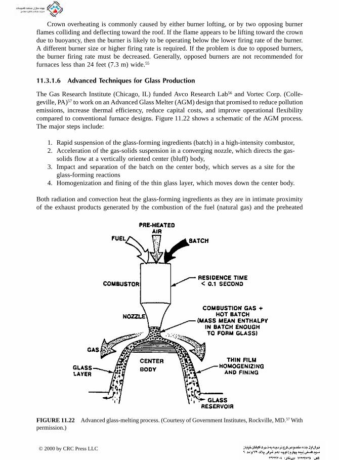
Crown overheating is commonly caused by either burner lofting, or by two opposing burnerflames colliding and deflecting toward the roof. If the flame appears to be lifting toward the crowndue to buoyancy, then the burner is likely to be operating below the lower firing rate of the burner.A different burner size or higher firing rate is required. If the problem is due to opposed burners,the burner firing rate must be decreased. Generally, opposed burners are not recommended forfurnaces less than 24 feet (7.3 m) wide.55
11.3.1.6 Advanced Techniques for Glass Production
The Gas Research Institute (Chicago, IL) funded Avco Research Lab56 and Vortec Corp. (Colle-geville, PA)57 to work on an Advanced Glass Melter (AGM) design that promised to reduce pollutionemissions, increase thermal efficiency, reduce capital costs, and improve operational flexibilitycompared to conventional furnace designs. Figure 11.22 shows a schematic of the AGM process.The major steps include:
1. Rapid suspension of the glass-forming ingredients (batch) in a high-intensity combustor,2. Acceleration of the gas-solids suspension in a converging nozzle, which directs the gas-
solids flow at a vertically oriented center (bluff) body,3. Impact and separation of the batch on the center body, which serves as a site for the
glass-forming reactions4. Homogenization and fining of the thin glass layer, which moves down the center body.
Both radiation and convection heat the glass-forming ingredients as they are in intimate proximityof the exhaust products generated by the combustion of the fuel (natural gas) and the preheated
FIGURE 11.22 Advanced glass-melting process. (Courtesy of Government Institutes, Rockville, MD.57 Withpermission.)
© 2000 by CRC Press LLC

air. The AGM process takes on the order of minutes, compared to conventional glass meltingprocesses which take on the order of hours up to days. The AGM claims 20% to 25% higherthermal efficiencies than conventional melting processes due to the improved heat transfer.
Abbasi et al. (1996) described a newly developed process known as oxygen-enriched air staging(OEAS).58 A schematic of the process for an end-port furnace is shown in Figure 11.23. A schematicfor the application of this process on a side-port furnace is shown in Figure 11.24. While the primaryobjective of the technology is to reduce NOx emissions (50% to 70% reduction was measured),there are also some effects on heat transfer. Since the preheated air flames are now initially fuel-rich, they are more luminous and therefore more radiative. The secondary oxygen added to theexhaust products completes the combustion before the gases exit the furnace. This secondarycombustion zone helps to spread out the heat transfer over a wider region in the furnace, whichhelps to make the heat flux more uniform.
11.3.2 CEMENT AND LIME
Cement and lime are commonly produced in rotary kilns. Pearce (1973) studied heat transfer inrotary kiln flames used in limestone production.59 Coal, gas, and oil flames were studied. Swirl
FIGURE 11.23 Plan view of oxygen-enriched air staging process on an end-port glass-melting furnace.(Courtesy of Government Institutes, Rockville, MD.58 With permission.)
FIGURE 11.24 Plan view of oxygen-enriched air-staging process on a side-port, glass-melting furnace.(Courtesy of Government Institutes, Rockville, MD.58 With permission.)
© 2000 by CRC Press LLC
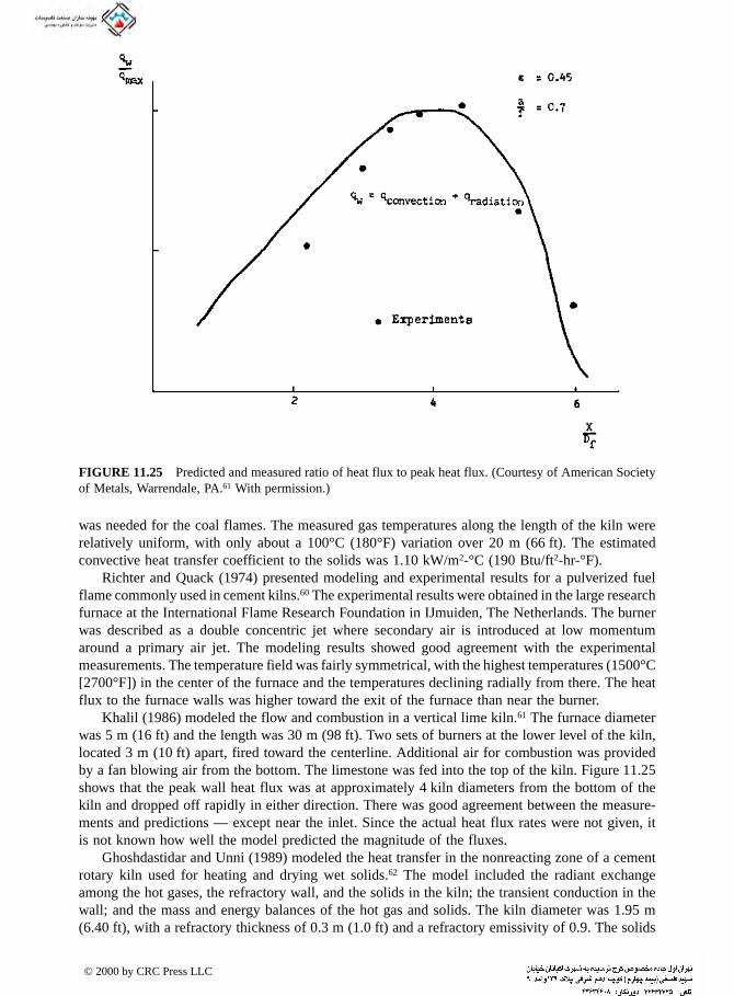
was needed for the coal flames. The measured gas temperatures along the length of the kiln wererelatively uniform, with only about a 100°C (180°F) variation over 20 m (66 ft). The estimatedconvective heat transfer coefficient to the solids was 1.10 kW/m2-°C (190 Btu/ft2-hr-°F).
Richter and Quack (1974) presented modeling and experimental results for a pulverized fuelflame commonly used in cement kilns.60 The experimental results were obtained in the large researchfurnace at the International Flame Research Foundation in IJmuiden, The Netherlands. The burnerwas described as a double concentric jet where secondary air is introduced at low momentumaround a primary air jet. The modeling results showed good agreement with the experimentalmeasurements. The temperature field was fairly symmetrical, with the highest temperatures (1500°C[2700°F]) in the center of the furnace and the temperatures declining radially from there. The heatflux to the furnace walls was higher toward the exit of the furnace than near the burner.
Khalil (1986) modeled the flow and combustion in a vertical lime kiln.61 The furnace diameterwas 5 m (16 ft) and the length was 30 m (98 ft). Two sets of burners at the lower level of the kiln,located 3 m (10 ft) apart, fired toward the centerline. Additional air for combustion was providedby a fan blowing air from the bottom. The limestone was fed into the top of the kiln. Figure 11.25shows that the peak wall heat flux was at approximately 4 kiln diameters from the bottom of thekiln and dropped off rapidly in either direction. There was good agreement between the measure-ments and predictions — except near the inlet. Since the actual heat flux rates were not given, itis not known how well the model predicted the magnitude of the fluxes.
Ghoshdastidar and Unni (1989) modeled the heat transfer in the nonreacting zone of a cementrotary kiln used for heating and drying wet solids.62 The model included the radiant exchangeamong the hot gases, the refractory wall, and the solids in the kiln; the transient conduction in thewall; and the mass and energy balances of the hot gas and solids. The kiln diameter was 1.95 m(6.40 ft), with a refractory thickness of 0.3 m (1.0 ft) and a refractory emissivity of 0.9. The solids
FIGURE 11.25 Predicted and measured ratio of heat flux to peak heat flux. (Courtesy of American Societyof Metals, Warrendale, PA.61 With permission.)
© 2000 by CRC Press LLC

had an emissivity of 0.95 and initially contained 18% water by weight. The convection coefficientbetween the inner refractory surface and the solids was chosen as 64 W/m2-K (11 Btu/ft2-hr-°F).The convection coefficient between the outer refractory surface and the surrounding environmentwas chosen as 10 W/m2-K (1.8 Btu/ft2-hr-°F). The predicted length to completely dry the solids inthe kiln was shorter than the measured length. There was good agreement between the actual andpredicted gas and solids temperatures as a function of axial position.
11.3.3 BRICKS, REFRACTORIES, AND CERAMICS
Bricks, refractories, and ceramics are often heated in a tunnel kiln (see Figure 11.26). The materialsto be heated — sometimes referred to as ware — are loaded onto cars and pushed through the kilnat regular intervals. The ware passes through three zones: preheating, firing, and cooling. In thepreheating zone, the ware is preheated by the exhaust products from the firing zone. The primaryfunction of the preheating zone is to remove moisture and burn out any organic material that mightbe present. In the firing zone, roof-mounted burners are fired in the free space around the ware.The function of this zone is to promote high-temperature chemical transformations (e.g., thedecomposition of carbonates), and to heat the ware to the sintering temperature. In the third zone —the cooling zone — the ware is cooled down by the incoming combustion air, which is simulta-neously preheated by the hot ware to improve the thermal efficiency of the system. Some of thepreheated air is removed from this zone and used in other parts of the plant.
An important aspect of the process is how the ware is stacked on the cars traveling throughthe tunnel kiln. The ware is arranged to maximize the convective heat and mass transfer of thecombustion gases flowing around it. The ware must be arranged so that all pieces receive adequateconvection and are properly treated. This precludes dense packing, which would not give adequateexposure to the innermost pieces of ware. Carvalho and Nogueira (1997) have modeled a tunnelkiln and shown how the stacking arrangement of the ware affects the load temperature.63
11.4 WASTE INCINERATION
Some of the material in this chapter section has been partially adapted from previous publica-tions.64,65 Incinerators are designed to burn — and in many cases destroy — waste materials thatmay sometimes be contaminated with hazardous substances. The waste materials usually have someheating value. However, nearly all incineration processes require a substantial amount of auxiliaryheat that is commonly generated by the combustion of hydrocarbon fuels such as natural gas oroil. An example of the important processes in a rotary kiln incinerator is shown in Figure 11.27.66
Incineration is a common method for treating waste materials. An ASME Committee onIndustrial and Municipal Wastes published a general guide to combustion in waste incineration.67
FIGURE 11.26 Tunnel kiln. (From Appl. Therm. Eng., 17(8-10), 921-933, 1997. With permission.)
© 2000 by CRC Press LLC

Seeker (1990)68 reviewed the use of combustion to dispose of waste materials and offered thefollowing advantages compared to other methods of disposal:
• Destruction of hazardous constituents such as organics and pathogens in the waste• Reduction of the volume and mass of the waste• Potential for energy recovery by burning the wastes having heating value• Making the waste unrecognizable from its original form (often a requirement for medical
waste)
The objective of most waste incineration processes is to destroy or burn any of the organic materialsin the waste, leaving only an inert residue. The waste combustion system consists of the followingcomponents:
1. Waste preparation and feeding,2. Combustion equipment,3. Heat recovery equipment,4. Air pollution control equipment,5. Ash/solid residue stabilization and disposal.
Wendt (1996) has also given a review of combustion in waste incineration.69 Although the paperdoes not specifically discuss heat transfer in waste incineration, it gives a good overview of thetechnology, with a specific emphasis on the pollutant emissions. Vrable (1987) has noted theimportance of recovering heat from waste incineration processes to improve thermal efficiency.70
Historically, air/fuel combustion has been used in waste processing to provide heat for thermaldestruction of solid, liquid, and gaseous waste streams. Examples include medical and municipalwaste (solid), spent solvents (liquid), and offgas or vent streams (gaseous). Oxygen-based combus-tion systems are becoming more common in waste processing applications.71 When traditional
FIGURE 11.27 Fundamental processes in rotary kiln incinerators. (Courtesy of CRC Press, Boca Raton, FL.66)
© 2000 by CRC Press LLC
air/fuel combustion systems have been modified for oxygen-enhanced combustion (OEC), manybenefits can be demonstrated. Typical improvements include higher destruction and removal effi-ciencies of the waste, increased thermal efficiency, increased processing rates, lower NOx andparticulates emissions, and less downtime for maintenance.
There are many benefits of using oxygen-enriched combustion in waste incineration. OEC hasbeen used in several different types of incineration applications to overcome thermal limitations inthe process.72 One example is a fixed rotary incinerator where kiln instabilities were produced byvariations in the incoming waste, which was sometimes cold and wet. The existing combustionsystem in the primary combustion chamber (PCC) was unable to handle these transient variations.O2 was injected into the kiln through a lance. The O2 flow was automatically controlled, based onfeedback from the temperature at the exit. This improved the kiln stability. It also improved therefractory life in the afterburner due to the more uniform temperature profile in the overall system.In general, OEC can be used to increase incinerator throughput of low-heating-value waste materials.
Another application of OEC to overcome thermal limitations is in thermal pyrolysis of municipalsolid waste or refuse-derived fuel (RDF).73 The N2 in air impedes the pyrolysis process, which iscommonly used to recover chemicals and energy. Using oxygen enrichment, high-quality char orgas can be produced from the high ash and moisture content fuels. OEC can increase the heatingvalue of the gas produced in gasification of municipal solid waste (MSW) by enhancing thedevolatilization and evolution of the gaseous products.73
In many cases, the volatilization characteristics of waste materials are unpredictable so thatincinerators are generally run with large amounts of excess air to ensure complete destruction ofthe volatiles.74 This excess air puts a large heat load on the incinerator. When some or all of theair is replaced with oxygen, some or all of the ballast nitrogen is eliminated, which reduces theheat load on the furnace and increases the thermal efficiency of the process. Eliminating ballastnitrogen also improves the destruction efficiency of the volatiles so that less excess oxygen isusually required, which further reduces the unproductive heat load on the incinerator. For an existingincinerator, this reduction in heat load may either mean more waste can be processed or the auxiliaryfuel consumption can be reduced. For a new incinerator, the equipment size and cost can be reduced.
The destruction and removal efficiency (DRE) is typically regulated for hazardous pollutantsas defined by the Resource Conservation and Recovery Act (RCRA). These pollutants include, forexample, polychlorinated biphenyls (PCBs) and principal organic hazardous constituents (POHCs)that may be found, for example, in contaminated soil. OEC can increase the DRE in an incinerationprocess. This is accomplished by a combination of increased residence time within the incineratorand higher gas temperatures. These are two of the “three T’s of incineration.” The higher residencetime is a result of the dramatically reduced flue gas volume that occurs when some or all of thecombustion air in an existing system is replaced with oxygen. For a given PCC, the gas velocitiesthrough the system will be lower with OEC compared to air/fuel combustion. Therefore, theresidence time will increase, which improves the mass transfer within the system. This increasesthe destruction efficiency of the hazardous pollutants in the process. The higher flame temperaturesassociated with oxygen-enhanced combustion ensure that all hydrocarbons in the incinerator willbe well above their ignition temperatures. Therefore, if there is sufficient oxygen for combustion,the hazardous pollutants should combust. The turbulence in the flame may be higher for OECcompared to conventional air/fuel combustion. However, the overall turbulence level in the com-bustion chamber will be reduced because of lower gas velocities. This must be offset by the increasedresidence time and higher gas temperatures in order to ensure adequate DRE. As will be shown,the DRE generally increases using OEC.
There are several potential problems that may result from OEC. Depending on the burnerdesign, oxygen-enhanced flames may be much hotter than air/fuel flames. This could lead topotential equipment damage due to overheating. Refractory damage may occur as a result oflocalized heating. A related problem is slagging. This may occur if the waste material is overheatedand begins to vitrify. Both of these overheating problems can be avoided by the choice of a properly
© 2000 by CRC Press LLC

designed burner, adequate waste flow through the incinerator to absorb the heat, and the properchoice of auxiliary heat input into the incinerator.
Another issue to consider when using OEC in an incinerator is the potentially detrimentaleffects of reducing the amount of convection in the combustion chambers resulting from thereduction in the nitrogen in the combustion products. Convection is important to both the heat andmass transfer within the incinerator. Gas circulation helps to homogenize the temperature in thecombustor, which minimizes hotspots that can damage refractories and cause nonuniform heating.A reduction in the gas volume could also reduce the mass transfer from the waste to the gas streamas volatiles are carried away from the surface of the waste. The gas flow over the waste materialin the incinerator carries away the volatiles so they can be incinerated and so that more volatilescan diffuse to the surface of the waste. Therefore, a reduction in the gas circulation within the gasspace of the combustor could potentially reduce the heat and mass transfer in the incinerator. Thisproblem is partially offset by the greater volume expansion of the gases because of the higher gastemperatures associated with OEC. Higher gas expansion increases the gas velocity in the chamber,which increases convection. Proper selection of equipment can also overcome this potential problemso that gas circulation in the incinerator is maintained using OEC.75 New incinerator designs forOEC could have a smaller combustion chamber compared to air/fuel systems for a given wastethroughput in order to achieve the desired average gas velocity.
11.4.1 TYPES OF INCINERATORS
This chapter section discusses some typical types of incinerators, including municipal solid wasteincinerators, mobile incinerators, transportable incinerators, and fixed incinerators.
11.4.1.1 Municipal Waste Incinerators
An example of a municipal solid waste (MSW) incineration process is shown in Figure 11.28. Theperformance of these incinerators can be improved using OEC.76 The economic incentives includeincreased waste-processing capacity, greater thermal efficiency, increased production in a waste-to-energy facility, reducing the demand on the exhaust system, and a smaller air pollution control
FIGURE 11.28 Municipal solid waste incinerator.
© 2000 by CRC Press LLC

system. Increased capacity can be particularly important for many waste processors that are at theirmaximum capacity, since it is usually difficult to obtain permits to build new facilities. Theenvironmental incentives include improved ash burnout, lower hydrocarbon emissions, lower CO,greater flexibility and control, and the ability to burn low-heating-value wastes such as dewateredsludge.
One of the earliest tests of oxygen enrichment in an MSW incinerator occurred at the Harrisburg,Pennsylvania, Waste-to-Energy Facility in 1987.77 The combustion air was enriched with 2% O2
(Ω = 0.23). The waste throughput, steam production, boiler efficiency, and sludge throughput allincreased. The flame stability improved with OEC. OEC has been used in an MSW incinerator toovercome thermal limitations.72 O2 was injected, through a diffuser, into the air plenums beneaththe waste bed. It was also injected, through a lance, directly onto the bed. This resulted in a 10%increase in the waste processing capacity, an increase in steam production, better overall boilerefficiency, and more complete burnout of the ash. Significant cost savings were realized in ashdisposal due to its lower volume and increased density.
The U.S. Environmental Protection Agency (EPA) sponsored a demonstration program toinvestigate OEC in a pilot-scale incinerator.78 With only 3% O2 enrichment (Ω = 0.24), the wasteprocessing rate increased by 24%. OEC did not seem to have any effect on the metal content ofthe ash. There were some concerns about higher hydrocarbon emissions at the higher throughputs.Further research was recommended. One important commercial consideration was the impact thistechnology might have on permitting. New or amended permits normally require a lengthy andusually costly review process.
11.4.1.2 Sludge Incinerators
A schematic of a sludge incineration process is shown in Figure 11.29. The biggest challenge insludge incineration is the large amount of energy required to evaporate the large quantity of watercontained in the sludge. The heating value of the sludge is minimal. Therefore, large quantities ofauxiliary fuel are required. Oxygen has been used to increase the capacity of a multiple-hearthsludge incinerator by 35% to 55% at a sewage treatment plant in Rochester, New York.79 Oxygenwas injected into the sludge-drying zone at a rate of 1 ton/hr through a series of lances. The amountof auxiliary natural gas fuel used to dry and burn the sludge was reduced by 57%. Emissions (permass of dry sludge) of total hydrocarbons, NOx, and CO were reduced by 58%, 62%, and 39%,respectively.
FIGURE 11.29 Sludge processing in a rotary kiln incinerator.
© 2000 by CRC Press LLC

11.4.1.3 Mobile Incinerators
Mobile incinerators are commonly used to clean up contaminated soil and water at Superfund sites.The entire incineration system, including the PCC, the SCC, and the pollution control equipment,is small enough to be transported over-the-road. It can be quickly set up and is usually preferredfor smaller sized cleanups. One of the first applications to use OEC in incineration was at theSuperfund cleanup site at the Denney Farm in McDowell, Missouri, starting in 1987.80 The EPAmobile incinerator was used, along with an OEC incineration technology that was later awardedthe prestigious Kirkpatrick Chemical Engineering Achievement Award for the results obtained atthis cleanup.81 Dioxin-contaminated liquids and solids were successfully treated. The OEC systemshowed impressive performance compared to the original air/fuel system. The throughput wasincreased by 171%, the specific fuel consumption decreased 61%, the residence time in the SCCincreased by 21%, CO spikes were reduced, while NOx levels were unaffected.
A more recent example is a trial burn to destroy PCB-containing electrical transformers andrelated contaminated materials.82 The waste material was fed into one end of a rotary kiln. A singleoxy/fuel burner, located at the kiln entrance, fired co-current with the feed material. The ash wascollected at the kiln exit. The combustion and process offgases from the kiln were fed into thesecondary chamber, which operated at a higher temperature than the primary chamber, to maximizedestruction of any remaining combustible gases. A block diagram of the process is shown inFigure 11.30. Before the contaminated soil was processed, the system was tested using surrogatewastes to ensure the emission requirements could be met. Three different series of tests wereconducted using various combinations of fuels and wastes. An oxy/propane burner in the PCC wasused to incinerate PCB-contaminated soil for the series A and B tests. The only difference betweenA and B was that propane and oil with 1% PCB, respectively, were used as fuels in the SCC. Inseries C, the PCC was not operated, while the fuel for the SCC was oil with 42% PCB.
Vesta Technology, Ltd. (Fort Lauderdale, FL) is a hazardous waste incineration company thatprovides on-site services throughout North America. Vesta’s mobile systems use high-temperaturerotary kiln incinerator technologies, coupled with innovative, proprietary designs for flue gasscrubbing. This proven technology destroys PCBs, dioxins, oil sludges, and other hazardous wasteswith DREs that exceed Resource Conservation and Recovery Act (RCRA) and Toxic SubstancesControl Act (TSCA) standards. Vesta has used this technology with both air/fuel and oxy/fuelsystems. The decision to try oxygen was mainly influenced by the requirement to reduce the fluegas volume within the system. The result was twofold. First, the lower flue gas velocity in the kilnresulted in less particulate carryover to the secondary combustion chamber (SCC) and the airpollution control system. Actual site operations showed that SCC clean-outs were reduced withthe lower flue gas flow, while actually increasing soil processing rates. Second, the flue gas residencetime in the SCC increased by 50%, which was expected to give higher DREs. Representative datafrom two similar remediation projects using the same equipment showed that the instantaneoussoil throughput rates increased by 50% using oxygen, compared to the air/fuel base case. Of greaterimportance, however was the overall average hourly throughput, which increased by 150% due tothe elimination of downtime for SCC particulate clean-out when using oxy/fuel. This rate enabledVesta to complete the remediation project 28 days ahead of schedule.83 The hourly NOx emissionswere reduced by 52%, while the pounds of NOx per ton of soil processed were reduced by 66%.
11.4.1.4 Transportable Incinerators
Transportable incinerators are also commonly used at Superfund cleanup sites. They are larger insize than mobile incinerators and take longer to set up. Therefore, they are used at larger sitesbecause of their increased processing capacity. The trend is to use these instead of mobile incin-erators.84 OEC has been used to maximize the transportable incinerator throughput by reducing thegas volume and improving the heat transfer performance. At the Bayou Bonfouca Superfund site
© 2000 by CRC Press LLC

in Saint Tammany Parish, Louisiana, cost savings were estimated to be nearly $3 million usingOEC instead of air/fuel.
The example given here shows how OEC reduced particulates in a transportable incinerator.Williams Environmental Services (WES), located in Auburn, Alabama, used an incineration systemconsisting of a co-current rotary kiln, a hot cyclone, a secondary combustion chamber, a quenchtower, baghouses, an induced draft fan, an acid gas absorber, and an exhaust stack. Air/fuel andoxy/fuel were used in this incineration system at two Superfund sites: a bankrupt wood-treatingoperation in Prentiss, Missouri, and at the Bog Creek Farm site in Howell, New Jersey. At thePrentiss site, the kiln was equipped with two air/fuel burners, while at the Bog Creek Farm site, asingle oxy/fuel burner was installed. The Prentiss site contained 9200 tons (8300 metric tons) ofcreosote-containing soil. The Bog Creek Farm site contained 25,000 tons (23,000 metric tons) ofsoil that contained VOCs, including benzene derivatives, chlorinated hydrocarbons, and semivolatileorganics such as naphthalene and phthalates.
OEC was selected for the Bog Creek site, due to the particulate emissions criteria set by theNew Jersey Department of Environmental Protection (NJDEP). The primary problem encounteredduring start-up at the Prentiss site was higher than expected fines carryover. About 50% of the ashoutput was from the air pollution control system. The Bog Creek site was located near the NewJersey coastline where the soil is naturally sandy. The existing particulate emission limit of0.03 grains per dry standard cubic foot (gr/dscf) or 0.07 grams per dry standard cubic meter (g/dscm)was reduced to a more rigorous standard of 0.015 gr/dscf (0.034 g/dscm) for this site, to preventcontaminated sand from entering the atmosphere. At a soil feed rate of 20 tons/hr (18 metrictons/hr), the equivalent Prentiss data indicated the estimated combined emissions (soil and metals)would have to be reduced by 65% to fall below the newly prescribed limit. OEC technology wasselected to meet the tougher particulate standard without causing a delay in the schedule.85 TheBog Creek site was the first Superfund site to use OEC incineration in the northeastern region ofthe U.S. and the first North American site to use OEC in a commercial, transportable incineratorfor the entire project. The processing rate increased using OEC. All emission and ash requirementswere satisfied. The site was cleaned up 60 days ahead of schedule. In this case, there was noreduction in NOx by using oxy/fuel, which was probably due to high air leakage into the kiln, asnoted by the increased oxygen in the flue gas.
11.4.1.5 Fixed Hazardous Waste Incinerators
Oxygen-enhanced combustion has been used to reduce NOx in a fixed based resource recoveryprocess.86 Giant Resource Recovery (GRR) is a subsidiary of the Giant Group, Ltd., which is involvedin cement manufacture and the use of waste materials as fuel and raw materials supplements. GRR
FIGURE 11.30 Mobile incineration system block diagram.
© 2000 by CRC Press LLC

processes creosote-contaminated soil through counter-current rotary kilns. By a patented process,the decontaminated soil is then used as a raw material for cement production, thus replacing acertain portion of the traditional feed material stream. The combustion products are ducted into thecement kilns. The kilns’ processing rates were limited by two factors. Since the contaminated soilwas high in moisture content and low in heating value, more heat transfer was required to increasethe throughput while ensuring the soil’s creosote concentration did not exceed permitted levels atthe kiln discharge. If the creosote concentration is too high, the soil has to be reprocessed beforebeing sent to the cement kiln. Second, the flue gas volume needed to be minimized to preventupsetting the cement kiln operation. These criteria were met by using an oxy/fuel burner. The kilnback-end temperature increased over 100°F (38°C) using an oxy/fuel burner. Over a range of severaltests, NOx emissions per ton of material processed were from 5% to 35% less using oxy/fuel. Inthis case, large amounts of air infiltration, evidenced by high O2 concentrations in the flue gas,limited the NOx reduction using oxygen.
Oxygen has been injected into rotary kiln incinerators and the secondary combustion chamberto reduce CO emissions by more than 60%, while increasing waste throughput by more than 15%at a German merchant incinerator.87 In the process, 530 ft3 (15 m3) of oxygen is injected for each84-lb (38-kg) drum of waste material.
11.4.2 HEAT TRANSFER IN WASTE INCINERATION
Owens et al. (1991) studied a pilot-scale rotary kiln incinerator, both computationally and experi-mentally.88 They studied the following parameters: kiln rotation rate (0.1 to 0.9 rpm), percent fillfraction (3 to 8), feed moisture content (0% to 20%), and inner wall temperature (190°C to 790°C[370 to 1450°F]). The experimental results showed that the moisture content of the solids signifi-cantly affects the temperature profile, the time for the solids to reach a given temperature is linearlydependent on the fill fraction, and the solids’ temperature is most sensitive at lower temperatureswhere convection heat transfer is dominant. The model results showed that geometrical scaling isnot sufficient, assuming a well-mixed bed is a reasonable approximation, and existing correlationsfor the wall-to-solids convection coefficient give useful bed temperature profiles. They found thecharacteristic time for convection-dominated heat transfer was:
(11.3)
where ρ is the density of the solids, cp is the specific heat of the dry solids, V is the solids volumeper unit length, hws is the convection heat transfer coefficient between the wall and the solids, andAconv is the area for convection heat transfer between the wall and the solids. The characteristictime for radiation-dominated heat transfer was:
(11.4)
where εs is the emissivity of the solids, Tg is the absolute temperature of the kiln gases, εg is theemissivity of the kiln gases, and Aw is the inner wall area excluding the area covered by the solids.
Kuo (1996) developed a simple lumped-parameter model to simulate a batch-fed solid wasteincinerator.89 The model could be used to study the response of an incinerator under a variety ofconditions and could also be used to control batch-fed incinerators, which are often controlled bythe skill and experience of the operators. One of the problems with batch-fed incinerators that arenot steady-state processes is that there is a possibility of emitting puffs of unburned hydrocarbons
τρ
convconv
=c V
h Ap
ws
τρσ
εε
ε ε
ε εrad =
−+
−( ) +
−( ) +[ ]⎧⎨⎪
⎩⎪
⎫⎬⎪
⎭⎪
c V
T A
A A
A A A
p
g
s
s s
s g g w
g s s g w
4
1 1
1
© 2000 by CRC Press LLC

due to changes in the waste feed. Therefore, control of the combustion air feed to the incineratoris important to get complete combustion. However, too much air reduces the combustion efficiency,which is important if the energy produced by the incinerator is recovered and used elsewhere, asis commonly the case. The challenge in batch-fed incineration processes is that the incoming wastecomposition is often in bags and unknown, so the amount of air required for combustion cannotbe determined a priori. The model assumes uniform temperature, pressure, and composition insidethe incinerator. Although the model is a fairly crude overall heat and material balance on the system,it is accurate and fast enough to be used in a control algorithm.
Bayley et al. (1996) developed a computer model to simulate the radiative, conductive, andconvective heat transfer effects in a waste incineration furnace designed to destruct hazardousliquids.90 The reason for the study was to determine if there would be a problem decontaminatingthe aluminum containers used to store the hazardous liquids. A schematic of the liquid-filled containerand heating process is shown in Figure 11.31. It is known that a potential “vapor explosion” hazardexists when processing molten metals (especially aluminum) in the presence of volatile liquids. Theconvective heat transfer to the upper surface of the container was modeled using:
(11.5)
The emissivity of the waste containers that had been in storage for some time was estimated to be0.1 to 0.5. The analysis showed that the aluminum would probably melt before the liquid wouldbe vaporized, which could lead to a vapor explosion, although the chances were not likely. Themost favorable condition to minimizing the chance of an explosion was by using an externalcontainer emissivity of 0.1 and an internal emissivity of 0.5. Since these conditions cannot beguaranteed, further analysis was recommended before proceeding with the original plan to decon-taminate the aluminum containers.
FIGURE 11.31 Schematic of waste liquid incineration process. (Courtesy of ASME, New York.90 Withpermission.)
Nu = 0 029 4 5 1 3. Re Pr
© 2000 by CRC Press LLC

REFERENCES
1. G.L. Shires, Furnaces, in International Encyclopedia of Heat and Mass Transfer, G.F. Hewitt, G.L.Shires, and Y.V. Polezhaev, Eds., CRC Press, Boca Raton, FL, 1997, 493-497.
2. A. Lehrman, C.D. Blumenschein, D.J. Doran, and S.E. Stewart, Steel plant fuels and water require-ments, in The Making, Shaping and Treating of Steel, 11th edition, Steelmaking and Refining Volume,R.J. Fruehan, Ed., AISE Steel Foundation, Pittsburgh, PA, 1998, 311-412.
3. R.J. Fruehan and C.L. Nassaralla, Alternative Oxygen Steelmaking Processes, in The Making, Shapingand Treating of Steel, 11th edition, Steelmaking and Refining Volume, R.J. Fruehan, Ed., AISE SteelFoundation, Pittsburgh, PA, 1998, 743-759.
4. M.D. Kistler and J.S. Becker, Ferrous metals, in Oxygen-Enhanced Combustion, C.E. Baukal, Ed.,CRC Press, Boca Raton, FL, 1998, 165-180.
5. J.A.T. Jones, B. Bowman, and P.A. Lefrank, Electric furnace steelmaking, in The Making, Shapingand Treating of Steel, 11th edition, Steelmaking and Refining Volume, R.J. Fruehan, Ed., AISE SteelFoundation, Pittsburgh, PA, 1998, 525-660.
6. M.B. Wells, and F.A. Vonesh, Oxy-fuel burner technology for electric arc furnaces, Iron & Steelmaker,13(11), 13-22, 1986.
7. H. Gripenberg, M. Brunner, and M. Petersson, Optimal distribution of oxygen in high efficiency arcfurnaces, Iron & Steel Engineer, 67(7), 33-37, 1990.
8. D.L. Schroeder, Use of energies in electric steelmaking shops, Electric Furnace Conf. Proceedings49, Iron & Steel Society, Warrendale, PA, 1991, 417-428.
9. K. Bergman and R. Gottardi, Design criteria for the modern UHP electric arc furnace with auxiliaries,Ironmaking and Steelmaking, 17(4), 282-287, 1990.
10. D.D. Battles and D.F. Knowles, New oxy-gas burner shows significant improvement in electric arcfurnace productivity, Proc. 1984 International Gas Research Conf., Govt. Institutes, Rockville, MD,1985, 796-802.
11. S.J. Sikirica, Field testing of oxygen-gas burner system on foundry and specialty steel electric arcfurnaces, Proc. 1986 International Gas Research Conf., T.L. Cramer, Ed., Govt. Institutes, Rockville,MD, 1987, 852-855.
12. J.R. Davila, A. Garrote, A.M. Gutierrez, P. Carnicer, L. Cobos, and I. Erauskin, New applications ofthe oxygas rotary furnace as a means of production in melting, Proc. of 1995 International GasResearch Conf., D.A. Dolenc, Ed., Govt. Institutes, Rockville, MD, 1996, 2764-2773.
13. D.H. Hubble, R.O. Russell, H.L. Vernon, and R.J. Marr, Steelmaking refractories, in The Making,Shaping and Treating of Steel, 11th edition, Steelmaking and Refining Volume, R.J. Fruehan, Ed.,AISE Steel Foundation, Pittsburgh, PA, 1998, 227-290.
14. G.J.W. Kor and P.C. Glaws, Ladle refining and vacuum degassing, in The Making, Shaping andTreating of Steel, 11th edition, Steelmaking and Refining Volume, R.J. Fruehan, Ed., AISE SteelFoundation, Pittsburgh, PA, 1998, 661-713.
15. C.E. Tomazin, E.A. Upton, and R.A. Willis, Steelmaking Conf. Proc., 69, Iron and Steel Society,Warrendale, PA, 1986, 223.
16. R. Klima, Improved knowledge of gas flow and heat transfer in reheating furnaces, Scandinavian J.Metallurgy (Suppl.), 26, 25-32, 1997.
17. G.S. Koch and J.H. Williams, Characterization of natural gas-fired and alternative steel reheat tech-nologies, in Industrial Combustion Technologies, M.A. Lukasiewicz, Ed., American Society of Metals,Warren, PA, 1986, 295-301.
18. K. Handa and Y. Tomita, Development of highly luminous gas burner and its application to saveenergy in the steel industry, Proc. 1984 International Gas Research Conf., Govt. Institutes, Rockville,MD, 1985, 729-739.
19. L.T. Walsh, M. Ho, M.G. Ding, Demonstrated fuel savings and uniform heating with 100% oxygenburners in a continuous steel reheat furnace, in Industrial Combustion Technologies, M.A.Lukasiewicz, Ed., American Society of Metals, Warren, PA, 1986, 259-265.
20. K.S. Chapman, S. Ramadhyani, and R. Viskanta, Modeling and analysis of heat transfer in a direct-fired continuous reheating furnace, in Heat Transfer in Combustion Systems, N. Ashgriz, J.G. Quin-tiere, H.G. Semerjian, and S.E. Slezak, Eds., New York, ASME HTD-Vol. 122, 35-43, 1989.
© 2000 by CRC Press LLC
21. Y.K. Lee, H.S. Park, and K.W. Cho, Effect of fuel gas preheating on combustion and heat transfer inreheating furnace, Proceedings of the 13th Energy Engineering World Congress, Energy & Environ-mental Strategies for the 1990s, Atlanta, GA, October 1990, 1991, chap. 78, 461-466.
22. K.S. Chapman, S. Ramadhyani, and R. Viskanta, Modeling and analysis of heat transfer in a direct-fired batch reheating furnace, in Heat Transfer Phenomena in Radiation, Combustion and Fires, R.K.Shah, Ed., ASME HTD-Vol. 106, 1989, 265-274.
23. J.M. Blanco and J.M. Sala, Improvement of the efficiency and working conditions for reheatingfurnaces through computational fluid dynamics, Industrial Heating, LXVI(5), 63-67, 1999.
24. F. Lisin and J.A. Marino, Heat transfer analysis in a batch steel reheat furnace, Industrial Heating,LXVI(10), 99-102, 1999.
25. C.D. Smith and D. Saha, Advances in Oxy/fuel Combustion: International Wrought Copper CouncilConference, Singapore, October 1997.
26. M.E. Ward, D. Knowles, S.R. Davis, and J. Bohn, Effect of combustion air preheat on a forge furnaceproductivity, Proc. 1984 International Gas Research Conf., Govt. Institutes, Rockville, MD, 1985,763-776.
27. S.Y. Salama and T.M. Desai, Electric induction versus gas metal heating: a case study, Proc. 1984International Gas Research Conf., Govt. Institutes, Rockville, MD, 1985, 777-786.
28. S. Takamichi, Development of high performance forging furnaces, Proc. 1998 International GasResearch Conf., Vol. V. Industrial Utilization and Power Generation, D. Dolenc, Ed., Govt. Institutes,Rockville, MD, 1998, 100-112.
29. D. Saha and C.E. Baukal, Nonferrous metals, in Oxygen-Enhanced Combustion, C.E. Baukal, Ed.,CRC Press, Boca Raton, FL, 1998, 181-214.
30. E.R. Bazarian, J.F. Heffron, and C.E. Baukal, Method for Reducing NOx Production During Air-FuelCombustion Processes, U.S. Patent 5,308,239 issued 03 May 1994.
31. M.W. Paget, J.F. Heffron, M. Lefebre, and C. Bazinet, A novel burner retrofit used to increaseproductivity in an aluminum rotary furnace and reduce baghouse loading, TMS Conference, 1994.
32. B. Phillips, D. Pakulski, M. Mazzei, E. Lepoutre, and H. Spoon, Use of air/oxy/fuel burners foraluminum dross processing, Industrial Heating, LX(3), 65-69, 1993.
33. D.J. Krichten, W.J. Baxter, and C.E. Baukal, Oxygen enhancement of burners for improved produc-tivity, EPD Congress 1997, Proceedings of the 1997 TMS Annual Meeting, B. Mishra, Ed., February9-13, Orlando, FL, 1997, 665-672.
34. L.D. Areaux and P. Corio, Aluminum scrap melting system provides high metal quality and meltyield, Industrial Heating, LXVI(8), 39-41, 1999.
35. C. Stala and D.L. Hindman, Gas-fired immersed ceramic tube aluminum melter, Proc. 1989 Interna-tional Gas Research Conf., T.L. Cramer, Ed., Govt. Institutes, Rockville, MD, 1990, 1453-1461.
36. M.E. Ward, R.E. Gildersleeve, S.J. Sikirica, and W.W. Liang, Application of a new ceramic recuperatortechnology for use on an aluminum remelt furnace, Proc. 1986 International Gas Research Conf.,T.L. Cramer, Ed., Govt. Institutes, Rockville, MD, 1987, 864-874.
37. R.A. Drake, Combustion Progress, Problems, Needs in the Glass Industry, in Industrial CombustionTechnologies, M.A. Lukasiewicz, Ed., American Society of Metals, Warren, PA, 1986, 23-25.
38. R. Gardon, A review of radiant heat transfer in glass, J. Amer. Ceramic Soc., 44(7), 305-312, 1961.39. R.J. Reid, What you should know about combustion, Glass Industry, 70(7), 24-35, 1989.40. V.K. Gegelashvili, V.V. Zhukovskii, and G.A. Svidzinskii, Separate admission of gas and air to a glass
furnace, Steklo Keram., No. 11, 38-39, 1968.41. A.I. Kukarkin, V.E. Dunduchenko, V.S. Marinskii, et al., A rational way to burn fuel in glass tank
furnaces, Steklo Keram., No. 6, 4-5, 1972.42. V.B. Kut’in, S.N. Gushchin, and V.G. Lisienko, Heat transfer in the cross-fired glass furnace, Glass
& Ceramics, 54(5-6), 135-138, 1997.43. V.G. Lisienko, V.B. Kut’in, and V.Ya. Dzyuzer, Influence of flame length and luminosity on heat
transfer in glass tank furnaces, Steklo Keram., No. 3, 6-8, 1981.44. V.B. Kut’in, S.N. Gushchin, and V.G. Lisienko, Heat exchange in the cross-fired glass furnace, Glass
& Ceramics, 54(5-6), 172-174, 1997.45. J. Cassiano, M.V. Heitor, and T.F. Silva, Combustion tests on an industrial glass-melting furnace,
Fuel, 73(10), 1638-1642, 1994.
© 2000 by CRC Press LLC

46. P.B. Eleazer and B.C. Hoke, Glass, in Oxygen-Enhanced Combustion, C.E. Baukal, Ed., CRC Press,Boca Raton, FL, 1998, 215-236.
47. J.T. Brown, 100% Oxygen-Fuel Combustion for Glass Furnaces, Collected Papers from the 51stConference on Glass Problems, 1990, 202-217.
48. A.G. Pincus, Ed., Combustion Melting in the Glass Industry, Magazines for Industry, New York, 1980.49. P.I. Booker, Developments in the use of oxygen in glass furnace combustion systems, Glass, 59(5),
172-178, 1982.50. D. Ertl and A. McMahon, Conversion of a fiberglass furnace from 100% electric to oxy/fuel com-
bustion, Proceedings from 54th Conference on Glass Problems, Oct. 1993, 186-190.51. S. Hope and S. Schemberg, Oxygen-fuel boosting on float furnaces, International Glass Review,
Spring/Summer, 1997, 63-66.52. M.G. Carvalho, D.F.G. Durão, and J.C.F. Pereira, Prediction of the flow, reaction and heat transfer in
an oxy-fuel glass furnace, Eng. Comput., 4(1), 23-34, 1987.53. V.I. Henry, W.J. Horbatch, C.V. Ramachandran, and L.W. Donaldson, Oxygen enrichment of a float
glass furnace. Phase I: System design and implementation, Proc. 1986 International Gas ResearchConf., T.L. Cramer, Ed., Govt. Institutes, Rockville, MD, 1987, 845-851.
54. D.E. Shamp and D.H. Davis, Application of 100% oxygen firing at Parkersburg, West Virginia,Collected Papers from the 51st Conference on Glass Problems, 1990, 218-239.
55. Slavejkov, A. G., Baukal, C. E., Joshi, M. L. and Nabors, J. K., Oxy/fuel glass melting with a highperformance burner, Ceram. Soc. Bull., 71(3), 340-343, 1992.
56. L.F. Westra and L.W. Donaldson, Development of an advanced glass melter system, Proc. 1986International Gas Research Conf., T.L. Cramer, Ed., Govt. Institutes, Rockville, MD, 1987, 889-897.
57. J. Hnat, D. Bender, L. Donaldson, A. Bendre, D. Tessari, J. Sacks, and A. Litka, Development of anadvanced gas-fired glass melting furnace, Proc. 1989 International Gas Research Conf., T.L. Cramer,Ed., Govt. Institutes, Rockville, MD, 1990, 1381-1390.
58. H.A. Abbasi, R.E. Grosman, L.W. Donaldson, C.F. Youssef, M.L. Joshi, and S.R. Hope, A low-NOxretrofit technology for regenerative glass melters, Proc. 1995 International Gas Research Conf., Vol.II, D.A. Dolenc, Ed., Govt. Institutes, Rockville, MD, 1996, 2322-2331.
59. K.W. Pearce, Heat transfer from rotary kiln flames, in Combustion Institute European Symposium1973, F.J. Weinberg, Ed., Academic Press, London, 1973, 663-668.
60. W. Richter and R. Quack, A mathematical model of a low-volatile pulverised fuel flame, in HeatTransfer in Flames, N.H. Afgan and J.M. Beer, Eds., Scripta Book Co., Washington, D.C., 1974, 95-109.
61. E.E. Khalil, Flow and combustion modeling of vertical lime kiln chambers, in Industrial CombustionTechnologies, M.A. Lukasiewicz, Ed., American Society of Metals, Warrendale, PA, 1986, 99-107.
62. P.S. Ghoshdastidar and V.K. Anandan Unni, Heat transfer in the non-reacting zone of a cement rotarykiln, in Heat Transfer Phenomena in Radiation, Combustion and Fires, R.K. Shah, Ed., New York,ASME HTD-Vol. 106, 1989, 113-122.
63. M. Carvalho and M. Nogueira, Improvement of energy efficiency in glass-melting furnaces, cementkilns and baking ovens, Appl. Therm. Eng., 17(8-10), 921-933, 1997.
64. C.E. Baukal, Oxygen-enhanced waste incineration, in Encyclopedia of Environmental Analysis andRemediation, R.A. Myers, Ed., Wiley, New York, 1998, 3283-3305.
65. C.E. Baukal, Waste incineration, in Oxygen-Enhanced Combustion, C.E. Baukal, Ed., CRC Press,Boca Raton, FL, 1998, 237-259.
66. A.M. Sterling, V.A. Cundy, T.W. Lester, A.N. Montestruc, J.S. Morse, C. Leger, and S. Acharya, In situsampling from an industrial-scale rotary kiln incinerator, in Emissions from Combustion Processes: Origin,Measurement, Control, R. Clement and R. Kagel, Eds., CRC Press, Boca Raton, FL, 1990, 319-335.
67. ASME Research Committee on Industrial and Municipal Wastes, Combustion Fundamentals for WasteIncineration, ASME, New York, 1974.
68. W.R. Seeker, Waste combustion, Twenty-Third Symposium (International) on Combustion, The Com-bustion Institute, Pittsburgh, PA, 1990, 867-885.
69. J.O.L. Wendt, Combustion science for incineration technology, Twenty-Fifth Symposium (Interna-tional) on Combustion, The Combustion Institute, Pittsburgh, PA, 1994, 277-289.
70. D.L. Vrable, Applications of high-temperature heat transfer — hazardous waste incineration, in HeatTransfer in High Technology and Power Engineering, W.-J. Yang and Y. Mori, Eds., Hemisphere,Washington, D.C., 1987.
© 2000 by CRC Press LLC

71. D. Fusaro, Incineration technology: still hot, getting hotter, Chemical Processing, 54(6), 26-32, 1991.72. S.D. Reese, Diverse experience using oxygen systems in waste incineration, presented at the Fourth
Annual National Symposium on Incineration of Industrial Wastes, February 28–March 2, Houston,Texas, 1990.
73. A.K. Gupta, Thermal destruction of solid wastes, J. Energy Resources Technology, 118, 187-192, 1996.74. G. Gitman, M. Zwecker, F. Kontz, and T. Wechsler, Oxygen enhancement of hazardous waste incin-
eration with the PYRETRON thermal destruction system, Thermal Processes, Vol. 1, H. M. Freeman,Ed., Technomic Publishing, Lancaster, PA, 1990, 207-225.
75. M.G. Ding, The use of oxygen for hazardous waste incineration, Thermal Processes, Vol. 1, H. M.Freeman, Ed., Technomic Publishing, Lancaster, PA, 1990, 181-190.
76. G.H. Shahani, D. Bucci, D. DeVincentis, S. Goff, and M.B. Mucher, Intensify waste combustion withoxygen enrichment, Chem. Eng., special supplement to 101(2), 18-24, 1994.
77. W.S. Strauss, J.A. Lukens, F.K. Young, and F.B. Bingham, Oxygen enrichment of combustion air ina 360 TPD mass burn refuse-fired waterwall furnace, Proc. of 1988 National Waste ProcessingConference, 13th Bi-Annual Conference, Philadelphia, PA, May 1-4, 1988, 315-320, 1988.
78. CSI Resource Systems and Solid Waste Assoc. of North America, Evaluation of Oxygen-EnrichedMSW/Sewage Sludge Co-Incineration Demonstration Program, U.S. Environmental ProtectionAgency Report EPA/600/R-94/145, Office of Research and Development, Cincinnati, OH, Sept. 1994.
79. G. Parkinson, Oxygen enrichment enhances sludge incineration, Chem. Eng., 103(12), 25, 1996.80. M.-D. Ho and M.G. Ding, Field testing and computer modeling of an oxygen combustion system,
J. Air Pollution & Waste Mgmt., 38(9), 1185-1191, 1988.81. N.P. Chopey, The tops in chemical engineering achievement, Chem. Eng., 96(12), 79-83, 1989.82. C.E. Baukal, L.L. Schafer, and E.P. Papadelis, PCB cleanup using an oxygen/fuel-fired mobile
incinerator, Envir. Progress, 13(3), 188-191, 1994.83. C.R. Griffith, PCB and PCP destruction using oxygen in mobile incinerators, Proceedings of the 1990
Incineration Conference, San Diego, May 4-18, 1990.84. P. Acharya, D. Fogo, and C. McBride, Process challenges in rotary kiln-based incinerators in soil
remediation projects, Envir. Progress, 15(4), 267-276, 1996.85. F.J. Romano and B.M. McLeod, The use of oxygen to reduce particulate emissions without reducing
throughput, Proceedings of 1990 Incineration Conference, paper 3.3, San Diego, May 14-18, 1990,589-596.
86. C.E. Baukal and F.J. Romano, Reducing NOx and particulates, Pollution Eng., 24(15), 76-79, 1992.87. K. Fouhy and G. Ondrey, Incineration: turning up the heat on hazardous waste, Chem. Eng., 101(5),
39-43, 1994.88. W.D. Owens, G.D. Silcox, J.S. Lighty, X.X. Deng, D.W. Pershing, V.A. Cundy, C.B. Leger, and A.L.
Jakway, Thermal analysis of rotary kiln incineration: comparison of theory and experiment, Comb.Flame, 86, 101-114, 1991.
89. J.T. Kuo, System simulation and control of batch-fed solid waste incinerators, in Heat Transfer inFire and Combustion Systems — 1994, W.W. Yuen and K.S. Ball, Eds., New York, ASME HTD-Vol.272, 55-62, 1994.
90. S.E. Bayley, R.T. Bailey, and D.C. Smith, Heat transfer analysis of hazardous waste containers withina furnace, in Combustion and Fire, ASME Proceedings of the 31st National Heat Transfer Conf.,Vol. 6, M. McQuay, K. Annamalai, W. Schreiber, D. Choudhury, E. Bigzadek, and A. Runchal, Eds.,ASME, New York, HTD-Vol. 328, 61-69, 1996.
91. Y. Kimura and K. Taniwaki, Development of immersion type aluminum melting furnace, Proc. 1989International Gas Research Conf., T.L. Cramer, Ed., Govt. Institutes, Rockville, MD, 1990,1470–1480.
© 2000 by CRC Press LLC
Advanced Combustion Systems
1212.1 INTRODUCTION
There are many types of so-called “advanced” combustion techniques. The term “advanced” is somewhat arbitrary, but here refers to technologies that are in use in industry (i.e., they are beyond the research and development stage), but are relatively new. The ones chosen for discussion here have a significant impact on the heat transfer from the flame to the load. This chapter describes technologies that are either in their infancy or are only used in a relatively narrow set of applications. In the future, the technologies described here may have broader appeal as advancements are made and as the technologies are accepted and implemented in industry.
12.2 OXYGEN-ENHANCED COMBUSTION
Most industrial heating processes require substantial amounts of energy, which are commonly generated by combusting hydrocarbon fuels such as natural gas or oil. Most combustion processes use air as the oxidant. In many cases, these processes can be enhanced using an oxidant that contains a higher proportion of O2 than that in air. This is known as oxygen-enhanced combustion, or OEC.1
Air consists of approximately 21% O2 and 79% N2 (by volume). One example of OEC is using an oxidant consisting of air blended with pure O2. Another example is using high-purity O2 as the oxidant — instead of air. This is usually referred to as oxy/fuel combustion.
New developments have made oxy/fuel combustion technology more amenable to a wide range of applications. In the past, the benefits of using oxygen did not always offset the added costs. New oxygen-generation technologies, such as pressure and vacuum swing adsorption, have sub-stantially reduced the cost of separating O2 from air. This has increased the number of applications where using oxygen to enhance performance is cost justified. Another important development is the increased emphasis on the environment. In many cases, OEC can substantially reduce pollutant emissions. This has also increased the number of cost-effective applications. The Gas Research Institute in Chicago, IL,2 and the U.S. Dept. of Energy3 have sponsored independent studies that predict that OEC will be a critical combustion technology in the very near future.
Historically, air/fuel combustion has been the conventional technology used in nearly all industrial heating processes. OEC systems are becoming more common in a variety of industries. When traditional air/fuel combustion systems have been modified for OEC, many benefits have been demonstrated. Typical improvements include increased thermal efficiency, increased process-ing rates, reduced flue gas volumes, and reduced pollutant emissions.
The use of oxygen in combustion has received relatively little attention from the academic combustion community. This may be for several reasons. Probably the most basic reason is the lack of research interest and funding to study OEC. The industrial gas companies that produce oxygen have been conducting research into OEC for many years; this has been mostly applied R&D. Very little basic research has been done, compared to air/fuel combustion, to study the fundamental processes in atmospheric flames utilizing OEC. The aerospace industry has done a considerable amount of work, for example, to study the high-pressure combustion of liquid oxygen and liquid hydrogen used to propel space vehicles. However, that work has little relevance to the low-pressure combustion of fuels other than hydrogen in industrial furnace applications. Another reason why minimal research has been done may be due to concerns about the safety issues of using oxygen, as well as the very high-temperature flames that may be encountered using OEC.
© 2000 by CRC Press LLC

Another reason may be a cost issue since the small quantities of oxygen that might be used can be relatively expensive. Handling oxygen cylinders takes more effort than using either a houseline
source of air or a small blower for the air used in small-scale flames.
Many industrial heating processes may be enhanced by replacing some or all of the air with high-purity oxygen.1,4 Typical applications include metal heating and melting, glass melting, and calcining. In a report5 done for the Gas Research Institute (1996), the following applications were identified as possible candidates for OEC:
• Processes that have high flue gas temperatures, typically in excess of 2000°F (1100°C)• Processes that have low thermal efficiencies, typically due to heat transfer limitations• Processes that have throughput limitations which could benefit from additional heat
transfer without adversely affecting product quality• Processes that have dirty flue gases, high NOx emissions, or flue gas volume limitations
When air is used as the oxidizer, only the O2 is needed in the combustion process. By eliminating N2 from the oxidizer, many benefits may be realized.
12.2.1 TYPICAL USE METHODS
Oxygen has been commonly used to enhance combustion processes in four primary ways: (1) adding O2 into the incoming combustion air stream, (2) injecting O2 into an air/fuel flame, (3) replacing the combustion air with high-purity O2, and (4) separately providing combustion air and O2 to the burner. These methods are discussed next.
12.2.1.1 Air Enrichment
Figure 12.1 shows an air/fuel process where the air is enriched with O2. This may be referred to as low-level O2 enrichment or premix enrichment. Many conventional air/fuel burners can be adapted for this technology.6 The O2 is injected into the incoming combustion air supply, usually through a diffuser to ensure adequate mixing. This is usually an inexpensive retrofit that can provide substantial benefits. Typically, the added O2 will shorten and intensify the flame. However, there may be some concerns if too much O2 is added to a burner designed for air/fuel. The flame shape may become unacceptably short. The higher flame temperature may damage the burner or burner block. The air piping may need to be modified for safety reasons to handle higher levels of O2. One of the earliest experimental studies reported on oxygen enrichment of combustion air was done at the International Flame Research Foundation (IJmuiden, The Netherlands) on oil flames.7
They also studied O2 lancing under the flame, which is discussed next.
FIGURE 12.1 Schematic of premixing O2 with air. (Courtesy of CRC Press, Boca Raton, FL.1)
© 2000 by CRC Press LLC

12.2.1.2 O2 Lancing
Figure 12.2 shows another method for enriching an air/fuel process with O2. As in the first method, this is also generally used for lower levels of O2 enrichment. However, oxygen lancing may have several advantages over air enrichment. No modifications to the existing air/fuel burner need to be made. Typically, the NOx emissions are lower using O2 lancing compared to premixing since this is a form of staging, which is a well-accepted technique for reducing NOx.8 Depending on the injection location, the flame shape may be lengthened by staging the combustion reactions. The flame heat release is generally more evenly distributed than with premix O2 enrichment. Under certain conditions, O2 lancing between the flame and the load causes the flame to be pulled toward the material. This improves the heat transfer efficiency. Therefore, there is less likelihood of overheating the air/fuel burner, the burner block, and the refractory in the combustion chamber. Another variant of this staging method involves lancing O2 not into the flame but somewhere else in the combustion chamber. One example of this technique is known as oxygen-enriched air staging, or OEAS. This O2 lancing technology is an inexpensive retrofit for existing processes. One potential disadvantage is the cost to add another hole in the combustion chamber for the lance. This includes both the installation cost and the lost productivity. However, the hole is typically very small.
One specific embodiment of O2 lancing is known as undershot enrichment, where O2 is lanced into the flame from below. The lance is located between the burner and the material being heated. While air enrichment increases the flame temperature uniformly, the undershot technique selectively enriches the underside of the conventional flame, thereby concentrating extra heat downward toward the material being heated. While the mixing of oxygen and combustion air is not as complete with undershot oxygen as with premixing, this disadvantage is often outweighed by the more effective placement of the extra heat. Another benefit is that the refractory in the roof of the furnace generally receives less heat compared to air enrichment. This usually increases the life of the roof.
12.2.1.3 Oxy/Fuel
Figure 12.3 shows a third method using OEC, commonly referred to as oxy/fuel combustion. In nearly all cases, the fuel and the oxygen remain separated inside the burner. They do not mix until reaching the outlet of the burner. This is commonly referred to as a nozzle-mix burner (see Figure 1.12), which produces a diffusion flame. There is no premixing of the gases — for safety reasons. Because of the extremely high reactivity of pure O2, there is the potential for an explosion if the gases are premixed. In this method, high-purity oxygen (>90% O2 by volume) is used to combust the fuel. As discussed later, there are several ways of generating the O2. In an oxy/fuel
FIGURE 12.2 Schematic of O2 lancing. (Courtesy of CRC Press, Boca Raton, FL.1)
© 2000 by CRC Press LLC
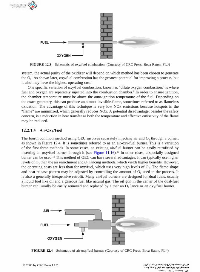
system, the actual purity of the oxidizer will depend on which method has been chosen to generate the O2. As shown later, oxy/fuel combustion has the greatest potential for improving a process, but it also may have the highest operating cost.
One specific variation of oxy/fuel combustion, known as “dilute oxygen combustion,” is where fuel and oxygen are separately injected into the combustion chamber.9 In order to ensure ignition, the chamber temperature must be above the auto-ignition temperature of the fuel. Depending on the exact geometry, this can produce an almost invisible flame, sometimes referred to as flameless oxidation. The advantage of this technique is very low NOx emissions because hotspots in the “flame” are minimized, which generally reduces NOx. A potential disadvantage, besides the safety concern, is a reduction in heat transfer as both the temperature and effective emissivity of the flame may be reduced.
12.2.1.4 Air-Oxy/Fuel
The fourth common method using OEC involves separately injecting air and O2 through a burner, as shown in Figure 12.4. It is sometimes referred to as an air-oxy/fuel burner. This is a variation of the first three methods. In some cases, an existing air/fuel burner can be easily retrofitted by inserting an oxy/fuel burner through it (see Figure 11.16).10 In other cases, a specially designed burner can be used.11 This method of OEC can have several advantages. It can typically use higher levels of O2 than the air enrichment and O2 lancing methods, which yields higher benefits. However, the operating costs are less than for oxy/fuel, which uses very high levels of O2. The flame shape and heat release pattern may be adjusted by controlling the amount of O2 used in the process. It is also a generally inexpensive retrofit. Many air/fuel burners are designed for dual fuels, usually a liquid fuel like oil and a gaseous fuel like natural gas. The oil gun in the center of the dual-fuel burner can usually be easily removed and replaced by either an O2 lance or an oxy/fuel burner.
FIGURE 12.3 Schematic of oxy/fuel combustion. (Courtesy of CRC Press, Boca Raton, FL.1)
FIGURE 12.4 Schematic of air-oxy/fuel burner. (Courtesy of CRC Press, Boca Raton, FL.1)
© 2000 by CRC Press LLC

With this method of using OEC, the oxidizer composition can be specified in an alternate way. Instead of giving the overall O2 concentration in the oxidizer, the oxidizer can be given as the
fraction of the total oxidizer, which is air and the fraction of the total oxidizer that is pure O2. The equivalent overall O2 in the oxidizer can be calculated as follows:
(12.1)
For example, the oxidizer may be specified as a blend of 60% O2 and 40% air. The ratio of O2 to air produces an equivalent of 39.8% overall O2 in the oxidizer.
12.2.2 OPERATING REGIMES
There are two common operating regimes for oxygen-enhanced combustion The first, or lower, regime is usually referred to as low-level enrichment (Ω < 0.30). This is commonly used in retrofit applications where only a few modifications need to be made to the existing combustion equipment. It is used when only incremental benefits are required. For example, in many cases, the production rate in a heating process can be significantly increased even with only relatively small amounts of oxygen enrichment. In most cases, air/fuel burners can successfully operate up to about Ω = 0.28 with no modifications.12 For Ω > 0.28, the flame may become unstable or the flame temperature may become too high for a burner designed to operate under air/fuel conditions. In some cases, it may be possible to make minor burner modifications to permit operation at slightly higher O2
concentrations.The other common operating regime is usually referred to as high-level enrichment, where
high-purity oxygen (Ω > 0.90) is used. This is used in higher temperature applications where the benefits of higher purity oxygen justify the added costs. The heating process is greatly intensified by the high-purity oxygen. In a retrofit situation, existing air/fuel burners are replaced by burners specifically designed to use the higher levels of O2.
It has only been in the last decade that a significant number of combustion systems have been operated in the intermediate oxygen regime, or medium-level enrichment (0.30 < Ω < 0.90). Again, these usually require specially designed burners or retrofits of existing burners.
12.2.3 HEAT TRANSFER BENEFITS
12.2.3.1 Increased Productivity
In most high-temperature heating processes, flame radiation is the dominant mode of heat transfer. Radiation is dependent on the fourth power of the absolute temperature (see Chapter 3). The higher temperatures associated with OEC increase the radiation from the flame to the load.13 This then increases the heat transfer to the load, which leads to increased material processing rates through the combustion chamber. Therefore, more material can be processed in an existing system, or new systems can be made smaller for a given processing rate. This is particularly important where space in a plant is limited. The environment benefits because of the reduction in the size of the equipment since less material and energy are needed in fabricating the combustion system. In order to take advantage of increased processing rates, the rest of the production system must be capable of handling the increased throughput. For example, the material handling system may need to be modified to handle the increased material flow rates.
The incremental costs of adding OEC to an existing combustion system are usually small compared to the capital costs of either expanding an existing system or adding new equipment in order to increase production. This has historically been one of the most popular reasons for using OEC. The advantage of OEC is that it can also be used intermittently to meet periodic demands
Ω = ( ) + ( )20 9
0 209 2
.. vol.% O vol.% Air
© 2000 by CRC Press LLC

for increased production. For example, if the demand for aluminum cans increases during the summer because of increased beverage consumption, OEC can be used at that time to meet the
increased demand for aluminum. If the demand decreases in the winter, then the OEC system could be throttled back or turned off until it is needed again. In most cases, using OEC would be much more economical than adding new equipment for increased capacity if the increased production demands are only temporary.
12.2.3.2 Higher Thermal Efficiencies
By using oxygen — instead of air — more energy goes into the load instead of being wasted in heating up N2. The energy needed to make O2 from air is only a small fraction of the energy used in the combustion process. Therefore, the overall process uses less energy for a given amount of production due to the higher available heat. In some instances, the cost of the oxygen can be offset by the reduction in fuel costs because of the increase in energy efficiency. This is often the case when OEC is used to supplement a process that uses electricity which is generally more expensive than fossil fuel combustion. In some cases, it is possible to substitute a less-expensive source of energy for an existing source of energy. For example, in the glass industry, furnaces are fueled primarily by oil or natural gas and commonly “boosted” with electrical energy. It has been shown that some or all of the more-expensive electrical energy can be eliminated by the proper use of OEC.
One common reason for using OEC is a reduction in the specific fuel consumption where less fuel is required for a given unit of production because of the improvement in available heat. A recent study projects that, for example, the cost of natural gas is expected to rise by about 10% from 1993 to the year 2000.4 At the same time, the cost of oxygen is expected to decrease by 10% due to lower electricity costs and improvements in oxygen production technology. The rising cost of fuel and the lowering cost of oxygen both make OEC a more attractive technology based solely on fuel savings.
Oxy/fuel combustion has been used in many applications in the steel industry, including both continuous and batch reheat furnaces, soaking pits, and ladle preheaters. Fuel savings of up to 60% have been reported.14,15 Typical fuel savings achieved by converting from air/fuel to oxy/fuel combustion are given in Table 12.1.16 Another example, from the glass industry, is that of Spectrum Glass, which reported fuel savings of 50% when it converted from air/fuel to oxy/fuel in its glass-melting furnaces.17
12.2.3.3 Higher Heat Transfer Efficiency
It has been argued that the efficiency of transferring heat from the flame to the load may be increased using OEC.18 In a nonluminous flame, the flame emissivity is higher for an oxygen-enhanced flame, compared to an air/fuel flame. This is due to the higher concentrations of CO2 and H2O, which are the gases that radiate in a flame.19 There is no radiation from the N2 in the flame. These effects are discussed in Chapter 3. Javorka (1990) gave an example of an oxygen-enrichment combustion system used to improve the heat transfer in a brass-smelting furnace.20 Farouk and Sidawi (1993) numerically showed that the radiative heat flux from oxy/natural gas flames is about an order of magnitude higher than for air/natural gas flames at the same firing rate.21
12.2.3.4 Increased Flexibility
There are many other benefits that can be achieved and are specific to a given process. OEC can increase the flexibility of a heating system.22 In some cases, a wider range of materials can be processed with OEC compared to air/fuel combustion. In other cases, OEC may be required if very high melting temperatures are required. For example, some ceramic and refractory products require firing temperatures of 2900°F (1600°C) and higher.23 Such temperatures are difficult if not impos-sible to achieve with standard air/fuel combustion with no air preheating. A heating system may
© 2000 by CRC Press LLC
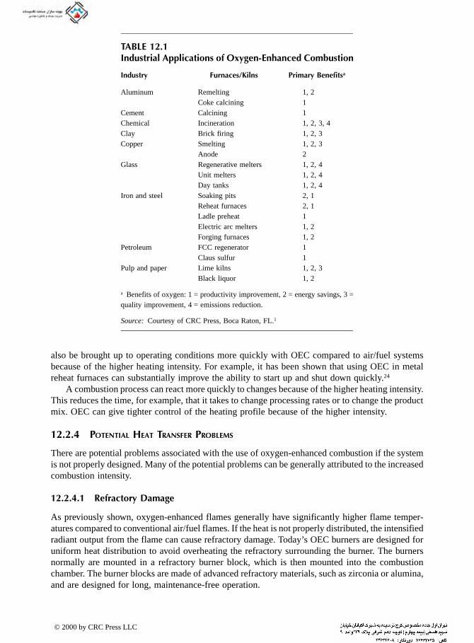
TABLE 12.1
also be brought up to operating conditions more quickly with OEC compared to air/fuel systems because of the higher heating intensity. For example, it has been shown that using OEC in metal reheat furnaces can substantially improve the ability to start up and shut down quickly.24
A combustion process can react more quickly to changes because of the higher heating intensity. This reduces the time, for example, that it takes to change processing rates or to change the product mix. OEC can give tighter control of the heating profile because of the higher intensity.
12.2.4 POTENTIAL HEAT TRANSFER PROBLEMS
There are potential problems associated with the use of oxygen-enhanced combustion if the system is not properly designed. Many of the potential problems can be generally attributed to the increased combustion intensity.
12.2.4.1 Refractory Damage
As previously shown, oxygen-enhanced flames generally have significantly higher flame temper-atures compared to conventional air/fuel flames. If the heat is not properly distributed, the intensified radiant output from the flame can cause refractory damage. Today’s OEC burners are designed for uniform heat distribution to avoid overheating the refractory surrounding the burner. The burners normally are mounted in a refractory burner block, which is then mounted into the combustion chamber. The burner blocks are made of advanced refractory materials, such as zirconia or alumina, and are designed for long, maintenance-free operation.
Industrial Applications of Oxygen-Enhanced Combustion
Industry Furnaces/Kilns Primary Benefitsa
Aluminum Remelting 1, 2Coke calcining 1
Cement Calcining 1Chemical Incineration 1, 2, 3, 4Clay Brick firing 1, 2, 3Copper Smelting 1, 2, 3
Anode 2Glass Regenerative melters 1, 2, 4
Unit melters 1, 2, 4Day tanks 1, 2, 4
Iron and steel Soaking pits 2, 1Reheat furnaces 2, 1Ladle preheat 1Electric arc melters 1, 2Forging furnaces 1, 2
Petroleum FCC regenerator 1Claus sulfur 1
Pulp and paper Lime kilns 1, 2, 3Black liquor 1, 2
a Benefits of oxygen: 1 = productivity improvement, 2 = energy savings, 3 = quality improvement, 4 = emissions reduction.
Source: Courtesy of CRC Press, Boca Raton, FL.1
© 2000 by CRC Press LLC

If the burner position and firing rate in the furnace are improperly chosen, refractory damage can result. For example, if the flame from an OEC burner is allowed to impinge directly on the
wall of a furnace, most typical refractory materials would be damaged. This can be prevented by the proper choice of the burner design and positioning. The flame length should not be so long that it impinges on the opposite wall. The burner mounting position in the furnace should be chosen to avoid aiming the flame directly at furnace refractories.
12.2.4.2 Nonuniform Heating
This is an important concern when retrofitting existing systems that were originally designed for air/fuel combustion. By intensifying the combustion process with OEC, there is the possibility of adversely affecting the heat and mass transfer characteristics within the combustion chamber. These issues are only briefly discussed here.
12.2.4.2.1 HotspotsOEC normally increases the flame temperature, which also increases the radiant heat flux from the flame to the load. If the increased radiant output is very localized, then there is the possibility of producing hotspots on the load. This could lead to overheating, which may damage or degrade the product quality. Today, burners for OEC have been specifically designed to avoid this problem. More information on burner design issues is given in Chapter 8.
12.2.4.2.2 Reduction in convectionAs shown in Figure 2.23, the total volume flow rate of exhaust products is significantly reduced using OEC. However, the average gas temperature is usually higher, but not by enough to offset the reduced gas flow rate. The convective heat transfer from the exhaust gases to the load may be reduced as a result. Another important aspect of convection is mass transfer. In some heating processes, especially those related to drying or removing volatiles, the reduced gas flow rate in the combustion chamber could adversely affect the mass transfer process. This can be offset using a burner that incorporates furnace gas recirculation, which increases the bulk volume flow inside the combustion chamber to help in removing volatiles that evolve from the load during the heating process.
12.2.5 INDUSTRIAL HEATING APPLICATIONS
Oxygen-enhanced combustion is used in a wide range of industrial heating applications. In general, OEC has been used in high-temperature heating and melting processes that are either very inefficient or not possible with air/fuel combustion. Table 12.1 shows some of the common reasons why OEC has been used in a variety of industrial applications.25 This chapter section is only intended to give a brief introduction to those applications that are broadly categorized here as metals, minerals, incineration, and other. These applications are discussed in detail elsewhere in the book.
12.2.5.1 Metals
Heating and melting metal was one of the first industrial uses of oxygen-enhanced combustion and continues to be an important application today. OEC has been widely used in both large integrated steel mills as well as in smaller mini-mills. It has also been used in the production of non-ferrous metals such as aluminum, brass, copper, and lead. Some of these applications are discussed in Chapter 11.
12.2.5.2 Minerals
Here, minerals refer to glass, cement, lime, bricks, and other related materials that require high-temperature heating and melting during their manufacture. OEC has been used in all of those applications. The use of OEC in glass is discussed in Chapter 11.
© 2000 by CRC Press LLC

12.2.5.3 Incineration
This is a relatively new area for OEC. Initially, OEC was used to enhance the performance of
portable incinerators used to clean up contaminated soil. It has also been used in municipal solid waste incinerators and in boilers burning waste fuels. The use of OEC in incineration is discussed in Chapter 11.
12.2.5.4 Other
OEC has been used in a wide variety of specialty applications that are not discussed in detail in this book. Some of these include gasifying organic materials and vitrifying residual ash,26 removing unburned carbon from fly ash,27 oxygen enrichment of fluid catalytic crackers,28 and oxygen enrich-ment of combustion air to combust H2S in sulfury recovery units (SRUs) to increase throughput.29
12.3 SUBMERGED COMBUSTION
Many types of submerged combustion processes have been tried, although it has been difficult to commercialize many of these due to the inherent problems with this type of process. Submerged combustion involves locating a burner in the bottom of a vessel filled with solids or liquids to be heated. The combustion products travel through the material and liberate their heat in a very efficient manner, which is usually the primary objective of this technique. Typical problems include finding the proper balance of flame intensity and gas velocity high enough to keep the material from flowing down into the burner, yet low enough that the gases do not bore a hole through the materials without effectively transferring their heat. A more mundane yet important problem is igniting the burner located underneath a bath or pile of material.
12.3.1 METALS PRODUCTION
One example of a submerged combustion process was designed and tested by Air Products and Chemicals, Inc. (Allentown, PA) with partial funding from the Gas Research Institute (Chicago, IL).30 The process was designed to use natural gas combusted with high-purity oxygen in a burner located at the bottom of a metal heating vessel. The objective of the process was to more econom-ically melt scrap metal using a fossil fuel by partially or fully replacing the electrical energy used in electric arc furnaces (EAF). The biggest challenge of the project was to design a submerged burner to operate over the entire regime from a packed bed of scrap metal to a full bath of molten metal. This was successfully achieved with a high-velocity burner design concept.31,32 As part of the research program, extensive testing was done using an oxy/fuel burner, firing vertically upward, mounted at the bottom of a 7.5-ton transfer ladle filled with scrap metal.33 A schematic of the system is shown in Figure 12.5. The scrap was hand-loaded into the vessel and included punchings, miscellaneous heavy scrap, and scrap containing instrumentation. The overall height of the load was 50 in. (130 cm) and the total weight was 2910 lb (1320 kg). Gas and scrap metal temperatures were measured at 15 different locations in the load at five different heights and three different radii. The firing rates ranged from 0.5 to 4 × 10⁶ Btu/hr (0.15 to 1.2 MW). Using the measured gas and scrap metal temperatures, the convective heat transfer coefficient ranged from 5 to 20 Btu/hr-ft2-°F(30 to 110 W/m2-K). The testing demonstrated the feasibility of using a submerged oxy/fuel burner to heat and melt scrap metal.
Another example of submerged combustion heating is in a pickling operation used for the surface treatment of metallic products. Chouinard and Bocherel (1990) described a submerged natural gas burner used to heat a tank containing a 15% sulfuric acid solution for pickling steel wire coils.34 A sketch of the system is shown in Figure 12.6. The exhaust products are distributed in a perforated tube array so they can bubble through the acid. Energy savings of up to 73%
© 2000 by CRC Press LLC

compared to conventional immersed steam coil heating techniques were demonstrated. This is due to the increased heat transfer effectiveness of bubbling the hot gases through the liquid pickling solution.
One type of vessel used to heat and melt in the metals industry is known as a shaft furnace. In that furnace, raw materials to be heated and melted are fed into the top of a tall refractory-lined vessel. Burners are located in the bottom of the vessel so that, similar to the process described above, the combustion products travel up through the packed bed of solids. However, one key distinction is that this process is continuous, with the melted raw materials being tapped off at the bottom of the shaft furnace. The process described previously is a batch process where the molten materials must be periodically tapped off by tipping the vessel on its side and pouring them out and then refilling the vessel with a new charge of raw scrap materials. In the shaft furnace, raw materials are added to the top on at least a semicontinuous, if not continuous, basis. One such shaft furnace is under development at the Institute of Gas Technology.35 Their process also incorporates heat recovery technology, where the combustion products leaving the top of the shaft are recycled down toward the burners where the heat is recovered and used to preheat the incoming combustion air. Advantages of this technology include uniform heat rates and high thermal efficiencies due to the counterflow heating of the packed bed and the heat recovery used to preheat the incoming combustion air.
Tatsumi (1996) described an immersion burner used to melt non-ferrous metals.36 The burner shown in Figure 12.7 is essentially a single-ended ceramic radiant tube. This can be used in applications like dip galvanizing, wire-rope galvanizing, and aluminum die casting. This new technology claims a 60% improvement over conventional nonsubmerged heating methods.
FIGURE 12.5 Submerged combustion steelmaking system experimental setup.
© 2000 by CRC Press LLC

12.3.2 MINERALS PRODUCTION
Olabin et al. (1998) described the use of a submerged combustion melting (SCM) process for use in producing mineral products.37 SCM was developed by the National Academy of Sciences of Ukraine and is now being extended to other applications, including the melting of cement kiln dust mixtures and sodium silicate using air/fuel and oxy/fuel firing. The SCM furnace is a bubbling type that is claimed to have better efficiency and lower capital costs compared to conventional melting furnaces. Burners are fired under a molten bath so that the gaseous combustion products bubble through the melt, which helps homogenize the mix. The high effective surface area promotes
FIGURE 12.6 Submerged combustion acid heating system. (Courtesy of Government Institutes, Rockville, MD.34 With permissiuon.)
FIGURE 12.7 Ceramic gas-fired immer-sion burner for heating non-ferrous metal. (Courtesy of Government Institutes, Rock-ville, MD.36 With permissiuon.)
© 2000 by CRC Press LLC
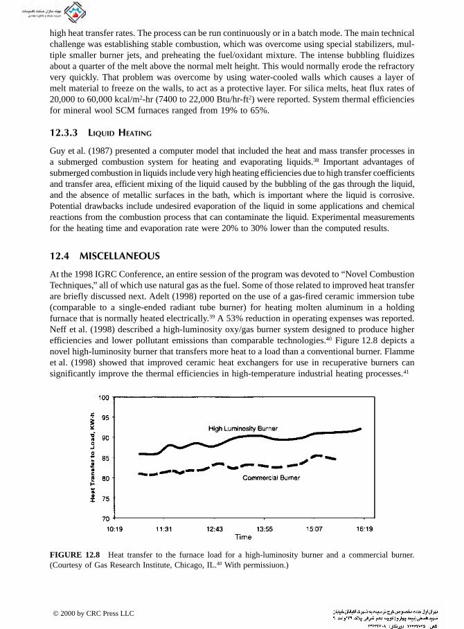
high heat transfer rates. The process can be run continuously or in a batch mode. The main technical challenge was establishing stable combustion, which was overcome using special stabilizers, mul-
tiple smaller burner jets, and preheating the fuel/oxidant mixture. The intense bubbling fluidizes about a quarter of the melt above the normal melt height. This would normally erode the refractory very quickly. That problem was overcome by using water-cooled walls which causes a layer of melt material to freeze on the walls, to act as a protective layer. For silica melts, heat flux rates of 20,000 to 60,000 kcal/m2-hr (7400 to 22,000 Btu/hr-ft2) were reported. System thermal efficiencies for mineral wool SCM furnaces ranged from 19% to 65%.
12.3.3 LIQUID HEATING
Guy et al. (1987) presented a computer model that included the heat and mass transfer processes in a submerged combustion system for heating and evaporating liquids.38 Important advantages of submerged combustion in liquids include very high heating efficiencies due to high transfer coefficients and transfer area, efficient mixing of the liquid caused by the bubbling of the gas through the liquid, and the absence of metallic surfaces in the bath, which is important where the liquid is corrosive. Potential drawbacks include undesired evaporation of the liquid in some applications and chemical reactions from the combustion process that can contaminate the liquid. Experimental measurements for the heating time and evaporation rate were 20% to 30% lower than the computed results.
12.4 MISCELLANEOUS
At the 1998 IGRC Conference, an entire session of the program was devoted to “Novel Combustion Techniques,” all of which use natural gas as the fuel. Some of those related to improved heat transfer are briefly discussed next. Adelt (1998) reported on the use of a gas-fired ceramic immersion tube (comparable to a single-ended radiant tube burner) for heating molten aluminum in a holding furnace that is normally heated electrically.39 A 53% reduction in operating expenses was reported. Neff et al. (1998) described a high-luminosity oxy/gas burner system designed to produce higher efficiencies and lower pollutant emissions than comparable technologies.40 Figure 12.8 depicts a novel high-luminosity burner that transfers more heat to a load than a conventional burner. Flamme et al. (1998) showed that improved ceramic heat exchangers for use in recuperative burners can significantly improve the thermal efficiencies in high-temperature industrial heating processes.41
FIGURE 12.8 Heat transfer to the furnace load for a high-luminosity burner and a commercial burner. (Courtesy of Gas Research Institute, Chicago, IL.40 With permissiuon.)
© 2000 by CRC Press LLC
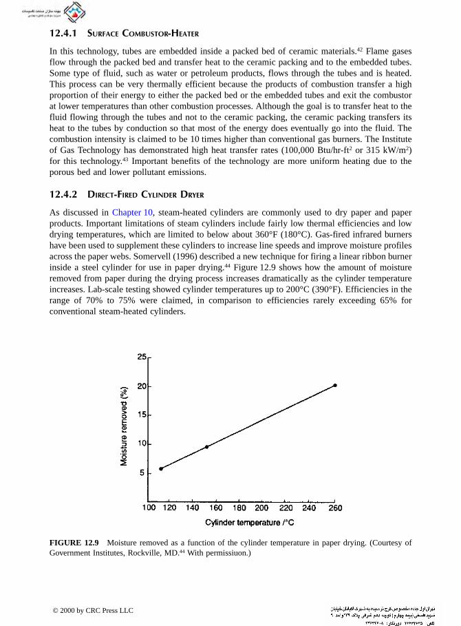
12.4.1 SURFACE COMBUSTOR-HEATER
In this technology, tubes are embedded inside a packed bed of ceramic materials.42 Flame gases
flow through the packed bed and transfer heat to the ceramic packing and to the embedded tubes. Some type of fluid, such as water or petroleum products, flows through the tubes and is heated. This process can be very thermally efficient because the products of combustion transfer a high proportion of their energy to either the packed bed or the embedded tubes and exit the combustor at lower temperatures than other combustion processes. Although the goal is to transfer heat to the fluid flowing through the tubes and not to the ceramic packing, the ceramic packing transfers its heat to the tubes by conduction so that most of the energy does eventually go into the fluid. The combustion intensity is claimed to be 10 times higher than conventional gas burners. The Institute of Gas Technology has demonstrated high heat transfer rates (100,000 Btu/hr-ft2 or 315 kW/m2) for this technology.43 Important benefits of the technology are more uniform heating due to the porous bed and lower pollutant emissions.
12.4.2 DIRECT-FIRED CYLINDER DRYER
As discussed in Chapter 10, steam-heated cylinders are commonly used to dry paper and paper products. Important limitations of steam cylinders include fairly low thermal efficiencies and low drying temperatures, which are limited to below about 360°F (180°C). Gas-fired infrared burners have been used to supplement these cylinders to increase line speeds and improve moisture profiles across the paper webs. Somervell (1996) described a new technique for firing a linear ribbon burner inside a steel cylinder for use in paper drying.44 Figure 12.9 shows how the amount of moisture removed from paper during the drying process increases dramatically as the cylinder temperature increases. Lab-scale testing showed cylinder temperatures up to 200°C (390°F). Efficiencies in the range of 70% to 75% were claimed, in comparison to efficiencies rarely exceeding 65% for conventional steam-heated cylinders.
FIGURE 12.9 Moisture removed as a function of the cylinder temperature in paper drying. (Courtesy of Government Institutes, Rockville, MD.44 With permissiuon.)
© 2000 by CRC Press LLC

REFERENCES
1. C.E. Baukal Ed., Oxygen-Enhanced Combustion, CRC Press, Boca Raton, FL, 1998.2. S.J. Williams, L.A. Cuervo, and M.A. Chapman, High-Temperature Industrial Process Heating: Oxy-
gen-Gas Combustion and Plasma Heating Systems, Gas Research Institute Report GRI-89/0256, Chicago, IL, July 1989.
3. A.S. Chace, H.R. Hazard, A. Levy, A.C. Thekdi, and E.W. Ungar, Combustion Research Opportunities for Industrial Applications — Phase II, U.S. Dept. of Energy Report DOE/ID-10204-2, Washington, D.C., 1989.
4. C.E. Baukal, P.B. Eleazer, and L.K. Farmer, Basis for enhancing combustion by oxygen enrichment, Industrial Heating, LIX(2), 22-24, 1992.
5. K.R. Benedek and R.P. Wilson, The Competitive Position of Natural-Gas in Oxy-Fuel Burner Appli-cations, Gas Research Institute Report no. GRI-96-0350, Chicago, IL, September 1996.
6. S.V. Joshi, J.S. Becker, and G.C. Lytle, Effects of oxygen enrichment on the performance of air-fuel burners, in Industrial Combustion Technologies, M.A. Lukasiewicz, Ed., Amer. Soc. Metals, 165-170, 1986.
7. R.R. Kissel and M. Michaud, International Flame Research Foundation: first experiments at IJmuiden on the combustion of oil using oxygen, J. Inst. Fuel, March, 1962, 109-120.
8. U.S. Environmental Protection Agency, Alternative Control Techniques Document — NOx Emissions from Utility Boilers, EPA Report EPA-453/R-94-023, Research Triangle Park, NC, 1994.
9. H. Kobayashi, Segregated Zoning Combustion, U.S. Patent 5,076,779, issued December 31, 1991.10. E.R. Bazarian, J.F. Heffron, and C.E. Baukal, Method for Reducing NOx Production During Air-Fuel
Combustion Processes, U.S. Patent 5,308,239, 1994.11. G.M. Gitman, Method and Apparatus for Generating Highly Luminous Flame, U.S. Patent 4,797,087,
1989.12. A.I. Dalton and D.W. Tyndall, Oxygen Enriched Air/Natural Gas Burner System Development, NTIS
Report PB91-167510, Springfield, VA, 1989.13. B.N. Gibbs and A. Williams, Fundamental aspects on the use of oxygen in combustion process — a
review, J. Inst. Energy, 56(427), 74-83, 1983.14. L.M. Farrell, T.T. Pavlack, and L. Rich, Operational and environmental benefits of oxy-fuel combustion
in the steel industry, Iron & Steel Engineer, 72(3), 35-42, 1995.15. L.K. Klingensmith, Direct-fired melter performance improved by gas/oxygen firing, Glass Industry,
67(4), 14–18, 1986.16. M.G. Ding and Z. Du, Energy and Environmental Benefits of Oxy-Fuel Combustion, Proc. of 1995
International Conference on Energy & Environment, Shanghai, China, May 1995, Begell House Inc., New York, 1995, 674-684.
17. S. Grisham, Oxy-conversion for a smaller furnace yields big results, American Glass Review, 117(6), 12, 1997.
18. H. Kobayashi, Oxygen Enriched Combustion System Performance Study, Phase I Interim/Final Report, Vol. I. Technical and Economic Analysis, U.S. Dept. of Energy Report DOE/ID/12597, Washington, D.C., March 1987.
19. H.C. Hottel and A.F. Sarofim, Radiative Transfer, McGraw-Hill, New York, 1967.20. D.J. Javorka, Brass smelter efficiency improved with new air-oxygen-fuel combustion system, Indus-
trial Heating, 57(5), 36-38, 1990.21. B. Farouk and M.M. Sidawi, Effects of nitrogen removal in a natural gas fired industrial furnace: a
three dimensional study, in Heat Transfer in Fire and Combustion Systems — 1993, B. Farouk, M. Pinar Menguc, R. Viskanta, C. Presser, and S. Chellaiah, Eds., New York, ASME HTD-Vol. 250, 173-183, 1993.
22. M. DeLucia, Oxygen enrichment in combustion processes: comparative experimental results from several application fields, J. Energy Resources Tech., 113, 122-126, 1991.
23. Industrial Heating Equipment Association, Combustion Technology Manual, fifth edition, Arlington, VA, 1994.
24. J. S. Becker and L.K. Farmer, Rapid fire heating system uses oxy-gas burners for efficient metal heating, Industrial Heating, 62(3), 74-78, 1995.
25. R.J. Reed, North American Combustion Handbook, third edition, 1997, Vol. II, Part 13.
© 2000 by CRC Press LLC

26. N.G. Bishop and G. Taylor, Method and Apparatus for Gasifying Organic Materials and Vitrifying Residual Ash, U.S. Patent 5,584,255, issued Dec. 17, 1996.
27. M.P. Martinez, Apparatus and Process for Removing Unburned Carbon in Fly Ash, U.S. Patent
5,555,821, issued Sept. 17, 1996.28. S. Tamhankar, R. Menon, T. Chou, R. Ramachandran, R. Hull, and R. Watson, Enrichment can decrease
NOx, SOx formation, Oil & Gas J., 94(10), 60-68, 1996.29. G. Parkinson, R. D’Aquino, and G. Ondrey, O2 Breathes New Life into Processes, Chem. Eng., 106(10),
28-31, 1999.30. M.B. DeGregorio and M.D. Lanyi, Development of a Submerged Combustion Steelmaking System:
Phases I and II, Gas Research Institute Report GRI-91/0067, Chicago, 1991.31. D.C. Winchester, L.K. Farmer, M.D. Lanyi, and C.E. Baukal, Accretion Controlling Tuyere, U.S.
Patent 5,431,709 issued 11 July 1995.32. D.C. Winchester, L.K. Farmer, M.D. Lanyi, and C.E. Baukal, Accretion Controlling Tuyere, U.S.
Patent 5,458,320 issued 17 October 1995.33. C.E. Baukal, M.D. Lanyi, and D.C. Winchester, Scrap preheating with a submerged oxy-fuel burner,
Iron & Steelmaking, 17(10), 51-56, 1990.34. J.-G. Chouinard and P. Bocherel, Submerged combustion system for acid tank heating, Proc. 1989
International Gas Research Conf., T.L. Cramer, Ed., Govt. Institutes, Rockville, MD, 1990, 1481-1488.35. M. J. Khinkis, Vertical Shaft Melting Furnace and Method of Melting, U.S. patent 4,877,449, issued
31 October 1989.36. N. Tatsumi, Development of non-ferrous metal melting technique by gas-fired ceramic immersion
heater, Proc. of 1995 International Gas Research Conf., D.A. Dolenc, Ed., Govt. Institutes, Rockville, MD, 1996, 2351-2358.
37. V. Olabin, A. Maximuk, D. Rue, and W. Kunc, Development of submerged combustion technology for producing mineral melts, Proc. of 1998 International Gas Research Conf., Vol. V. Industrial Utilization, D.A. Dolenc, Ed., Gas Research Institute, Chicago, 1998, 685-695.
38. C. Guy, P.J. Carreau, and J. Paris, Heating and evaporation of liquids by submerged combustion, Proc. 1986 International Gas Research Conf., T.L. Cramer, Ed., Govt. Institutes, Rockville, MD, 1987, 903-912.
39. M. Adelt, Aluminum holding with ceramic immersion tubes, Proc. of 1998 International Gas Research Conf., Vol. V: Industrial Utilization, D.A. Dolenc, Ed., Gas Research Institute, Chicago, 1998, 15-23.
40. D. Neff, P. Mohr, J. Gaddone, A. Fridman, S. Nestor, R. Viskanta, R. Jain, D. Rue, and O. Loo, High-luminosity, low-NOx oxy-natural gas burner for high-temperature furnaces, Proc. of 1998 International Gas Research Conf., Vol. V: Industrial Utilization, D.A. Dolenc, Ed., Gas Research Institute, Chicago, 1998, 34-44.
41. M. Flamme, M. Boß, M. Brune, A. Lynen, J. Heym, J.A. Wünning, J.G. Wünning, and H.J. Dittman, Improvement of energy saving with new ceramic self-recuperative burners, Proc. of 1998 International Gas Research Conf., Vol. V: Industrial Utilization, D.A. Dolenc, Ed., Gas Research Institute, Chicago, 1998, 88-99.
42. M. J. Khinkis, Gas-Fired, Porous Matrix, Surface Combustor-Fluid Heater, U.S. patent 5,375,563, issued 27 December 1994.
43. Institute of Gas Technology, Compact Ultra-Low-Emission Process Heater, brochure, Chicago, IL, 1998.
44. T.R. Somervell, Experimental evaluation of direct gas fired drying cylinder performance, Proc. of 1995 International Gas Research Conf., D.A. Dolenc, Ed., Govt. Institutes, Rockville, MD, 1996, 2359-2368.
© 2000 by CRC Press LLC

Appendix A
Reference Sources for Further InformationThe list below is not intended to be exhaustive as there are other journals that may occasionally have papers on industrial combustion, but the ones listed here are more likely to have such articles.
1. Heat transfer journals
Applied Thermal Engineering Calore é Tecnologica (Heat and Technology) Experimental Heat Transfer Experimental Thermal and Fluid Science Heat Transfer — Japanese Research Heat Transfer — Russian Research International Communications in Heat and Mass Transfer International Journal of Heat and Fluid Flow International Journal of Heat and Mass Transfer Journal of Heat Transfer Journal of Thermophysics and Heat Transfer Wärme und Stoffübertragung (Heat and Mass Transfer)
2. Combustion journals
Combustion and Flame Combustion Science and Technology Fuel (formerly Journal of the Institute of Fuel) Journal of the Institute of Energy Progress in Energy and Combustion Science
3. Industrial trade journals
Ceramic Industry Glass Glass Industry Glass Technology Hydrocarbon Processing Industrial Heating Light Metals Oil & Gas Journal Process Heating
© 2000 by CRC Press LLC

4. Miscellaneous sources
American Flame Research Committee conference proceedings
American Society of Mechanical Engineers (ASME) combustion conference proceed-ings (New York, NY)Gas Research Institute reports (Chicago, IL)International Flame Research Foundation reports (IJmuiden, the Netherlands)International (Symposia) on Combustion proceedings (The Combustion Institute, Pittsburgh, PA)U.S. Dept. of Energy reports (Washington, D.C.)U.S. Patent & Trademark Office (Washington, D.C.)
© 2000 by CRC Press LLC

Appendix B
Common Conversions1 Btu = 252.0 cal 1 in. = 2.540 cm
1055 J 25.40 mm1 Btu/ft3 = 0.00890 cal/cm3 1 J = 0.000948 Btu
0.0373 MJ/m3 0.239 cal1 Btu/hr = 0.0003931 hp 1 W/sec
0.2520 kcal/hr 1 kcal = 3.968 Btu0.2931 W 1000 cal
1,000,000 Btu/hr = 0.293 MW 4187 J1 Btu/hr-ft2 = 0.003153 kW/m2 1 kcal/hr = 3.968 Btu/hr1 Btu/hr-ft-°F = 1.730 W/m-K 1.162 J/sec1 Btu/hr-ft2-°F = 5.67 W/m2-K 1 kcal/m3 = 0.1124 Btu/ft3
1 Btu/lb = 0.5556 cal/g 4187 J/m3
2326 J/kg 1 kg = 2.205 lb1 Btu/lb-°F = 1 cal/g-°C 1 kg/hr-m = 0.00278 g/sec-cm
4187 J/kg-K 0.672 lb/hr-ft1 cal = 0.003968 Btu 1 kg/m3 = 0.06243 lb/ft3
4.187 J 1 kW = 3413 Btu/hr1 cal/cm2-sec = 3.687 Btu/ft2-sec 1.341 hp
41.87 kW/m2 660.6 kcal/hr1 cal/cm-sec-°C = 241.9 Btu/ft-hr-°F 1 kW/m2 = 317.2 Btu/hr-ft2
418.7 W/m-K 1 kW/m2-°C = 176.2 Btu/hr-ft2-°F1 cal/g = 1.80 Btu/lb 1 lb = 0.4536 kg
4187 J/kg 1 lb/ft3 = 0.0160 g/cm3
1 cal/g-°C = 1 Btu/lb-°F 16.02 kg/m3
4187 J/kg-K 1 lbm/hr-ft = 0.413 centipoise1 centipoise = 2.421 lbm/hr-ft 1 m = 3.281 ft1 cm2/sec = 100 centistokes 1 mm = 0.03937 in.
3.874 ft2/hr 1 m2/sec = 10.76 ft2/sec1 ft = 0.3048 m 1 mton = 1000 kg1 ft2/sec = 0.0929 m2/sec 2205 lb1 g/cm3 = 1000 kg/m3 1 MW = 3,413,000 Btu/hr
62.43 lb/ft3 1000 kW0.03613 lb/in.3 1 therm = 100,000 Btu
1 hp = 33,000 ft-lb/min 1 W = 1 J/sec550 ft-lb/sec 1 W/m-K = 0.5778 Btu/ft-hr-°F641.4 kcal/hr745.7 W
© 2000 by CRC Press LLC

TEMPERATURE CONVERSIONS
°C = 5/9 (°F – 32) °F = 9/5 (°C + 32)
K = °C + 273.15 °R = °F + 459.67
© 2000 by CRC Press LLC
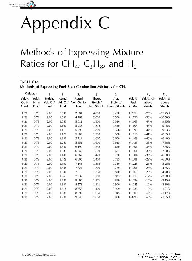
Appendix C
Methods of Expressing Mixture Ratios for CH4, C3H8, and H2
TABLE C1aMethods of Expressing Fuel-Rich Combustion Mixtures for CH4
Oxidizer S S1 S2 φ λ XA XO2
Vol.% O2 in Oxid.
Vol.% N2 in Oxid.
Stoich. Vol. O2 /
Fuel
Actual Vol. O2 /
Fuel
Actual Vol. Oxid./
Fuel
Theor. Stoich./
Act. Stoich.
Act. Stoich./
Theor. Stoich.
Vol. % Fuel
in Mix
Vol.% Air above Stoich.
Vol.% O2 above Stoich.
0.21 0.79 2.00 0.500 2.381 4.000 0.250 0.2958 –75% –15.75%0.21 0.79 2.00 1.000 4.762 2.000 0.500 0.1736 –50% –10.50%0.21 0.79 2.00 1.053 5.012 1.900 0.526 0.1663 – 47% –9.95%0.21 0.79 2.00 1.100 5.238 1.818 0.550 0.1603 – 45% –9.45%0.21 0.79 2.00 1.111 5.290 1.800 0.556 0.1590 – 44% –9.33%0.21 0.79 2.00 1.177 5.602 1.700 0.588 0.1515 – 41% –8.65%0.21 0.79 2.00 1.200 5.714 1.667 0.600 0.1489 – 40% –8.40%0.21 0.79 2.00 1.250 5.952 1.600 0.625 0.1438 –38% –7.88%0.21 0.79 2.00 1.300 6.190 1.538 0.650 0.1391 –35% –7.35%0.21 0.79 2.00 1.333 6.349 1.500 0.667 0.1361 –33% –7.00%0.21 0.79 2.00 1.400 6.667 1.429 0.700 0.1304 –30% –6.30%0.21 0.79 2.00 1.429 6.805 1.400 0.715 0.1281 –29% –6.00%0.21 0.79 2.00 1.500 7.143 1.333 0.750 0.1228 –25% –5.25%0.21 0.79 2.00 1.538 7.324 1.300 0.769 0.1201 –23% – 4.85%0.21 0.79 2.00 1.600 7.619 1.250 0.800 0.1160 –20% – 4.20%0.21 0.79 2.00 1.667 7.937 1.200 0.833 0.1119 –17% –3.50%0.21 0.79 2.00 1.700 8.095 1.176 0.850 0.1099 –15% –3.15%0.21 0.79 2.00 1.800 8.571 1.111 0.900 0.1045 –10% –2.10%0.21 0.79 2.00 1.818 8.657 1.100 0.909 0.1036 –9% –1.91%0.21 0.79 2.00 1.889 8.995 1.059 0.945 0.1000 –6% –1.17%0.21 0.79 2.00 1.900 9.048 1.053 0.950 0.0995 –5% –1.05%
© 2000 by CRC Press LLC

TABLE C1b
Methods of Expressing Stoichiometric and Fuel-Lean Combustion Mixtures for CH4
Oxidizer S S1 S2 φ λ XA XO2
Vol.% O2 in Oxid.
Vol.% N2 in Oxid.
Stoich. Vol. O2 /
Fuel
Actual Vol. O2 /
Fuel
Actual Vol. Oxid./
Fuel
Theor. Stoich./
Act. Stoich.
Act. Stoich./
Theor. Stoich.
Vol. % Fuel
in Mix
Vol.% Air above Stoich.
Vol.% O2 above Stoich.
0.21 0.79 2.00 2.000 9.524 1.000 1.000 0.0950 0% 0.00%0.21 0.79 2.00 2.095 9.976 0.955 1.048 0.0911 5% 1.00%0.21 0.79 2.00 2.100 10.000 0.952 1.050 0.0909 5% 1.05%0.21 0.79 2.00 2.124 10.114 0.942 1.062 0.0900 6% 1.30%0.21 0.79 2.00 2.190 10.429 0.913 1.095 0.0875 10% 2.00%0.21 0.79 2.00 2.200 10.476 0.909 1.100 0.0871 10% 2.10%0.21 0.79 2.00 2.221 10.576 0.900 1.111 0.0864 11% 2.32%0.21 0.79 2.00 2.286 10.886 0.875 1.143 0.0841 14% 3.00%0.21 0.79 2.00 2.300 10.952 0.870 1.150 0.0837 15% 3.15%0.21 0.79 2.00 2.400 11.429 0.833 1.200 0.0805 20% 4.20%0.21 0.79 2.00 2.500 11.905 0.800 1.250 0.0775 25% 5.25%0.21 0.79 2.00 2.600 12.381 0.769 1.300 0.0747 30% 6.30%0.21 0.79 2.00 2.667 12.698 0.750 1.333 0.0730 33% 7.00%0.21 0.79 2.00 2.700 12.857 0.741 1.350 0.0722 35% 7.35%0.21 0.79 2.00 2.800 13.333 0.714 1.400 0.0698 40% 8.40%0.21 0.79 2.00 2.859 13.614 0.700 1.430 0.0684 43% 9.02%0.21 0.79 2.00 2.900 13.810 0.690 1.450 0.0675 45% 9.45%0.21 0.79 2.00 3.000 14.286 0.667 1.500 0.0654 50% 10.50%0.21 0.79 2.00 3.500 16.667 0.571 1.750 0.0566 75% 15.75%0.21 0.79 2.00 4.000 19.048 0.500 2.000 0.0499 100% 21.00%0.30 0.70 2.00 2.000 6.667 1.000 1.000 0.1304 0% 0.00%0.40 0.60 2.00 2.000 5.000 1.000 1.000 0.1667 0% 0.00%0.50 0.50 2.00 2.000 4.000 1.000 1.000 0.2000 0% 0.00%0.60 0.40 2.00 2.000 3.333 1.000 1.000 0.2308 0% 0.00%0.70 0.30 2.00 2.000 2.857 1.000 1.000 0.2593 0% 0.00%0.80 0.20 2.00 2.000 2.500 1.000 1.000 0.2857 0% 0.00%0.90 0.10 2.00 2.000 2.222 1.000 1.000 0.3103 0% 0.00%1.00 0.00 2.00 2.000 2.000 1.000 1.000 0.3333 0% 0.00%
© 2000 by CRC Press LLC

TABLE C2a
Methods of Expressing Fuel-Rich Combustion Mixtures for C3H8
Oxidizer S S1 S2 φ λ XA XO2
Vol.% O2 in Oxid.
Vol.% N2 in Oxid.
Stoich. Vol. O2 /
Fuel
Actual Vol. O2 /
Fuel
Actual Vol. Oxid./
Fuel
Theor. Stoich./
Act. Stoich.
Act. Stoich./
Theor. Stoich.
Vol. % Fuel
in Mix
Vol.% Air above Stoich.
Vol.% O2 above Stoich.
0.21 0.79 5.00 1.250 5.952 4.000 0.250 0.1438 –75% –15.75%0.21 0.79 5.00 2.500 11.905 2.000 0.500 0.0775 –50% –10.50%0.21 0.79 5.00 2.631 12.530 1.900 0.526 0.0739 – 47% –9.95%0.21 0.79 5.00 2.750 13.095 1.818 0.550 0.0709 – 45% –9.45%0.21 0.79 5.00 2.778 13.226 1.800 0.556 0.0703 – 44% –9.33%0.21 0.79 5.00 2.941 14.006 1.700 0.588 0.0666 – 41% –8.65%0.21 0.79 5.00 3.000 14.286 1.667 0.600 0.0654 – 40% –8.40%0.21 0.79 5.00 3.125 14.881 1.600 0.625 0.0630 –38% –7.88%0.21 0.79 5.00 3.250 15.476 1.538 0.650 0.0607 –35% –7.35%0.21 0.79 5.00 3.333 15.873 1.500 0.667 0.0593 –33% –7.00%0.21 0.79 5.00 3.500 16.667 1.429 0.700 0.0566 –30% –6.30%0.21 0.79 5.00 3.573 17.012 1.400 0.715 0.0555 –29% –6.00%0.21 0.79 5.00 3.750 17.857 1.333 0.750 0.0530 –25% –5.25%0.21 0.79 5.00 3.845 18.310 1.300 0.769 0.0518 –23% – 4.85%0.21 0.79 5.00 4.000 19.048 1.250 0.800 0.0499 –20% – 4.20%0.21 0.79 5.00 4.167 19.842 1.200 0.833 0.0480 –17% –3.50%0.21 0.79 5.00 4.250 20.238 1.176 0.850 0.0471 –15% –3.15%0.21 0.79 5.00 4.500 21.429 1.111 0.900 0.0446 –10% –2.10%0.21 0.79 5.00 4.545 21.643 1.100 0.909 0.0442 –9% –1.91%0.21 0.79 5.00 4.723 22.488 1.059 0.945 0.0426 –6% –1.17%0.21 0.79 5.00 4.750 22.619 1.053 0.950 0.0423 –5% –1.05%
© 2000 by CRC Press LLC
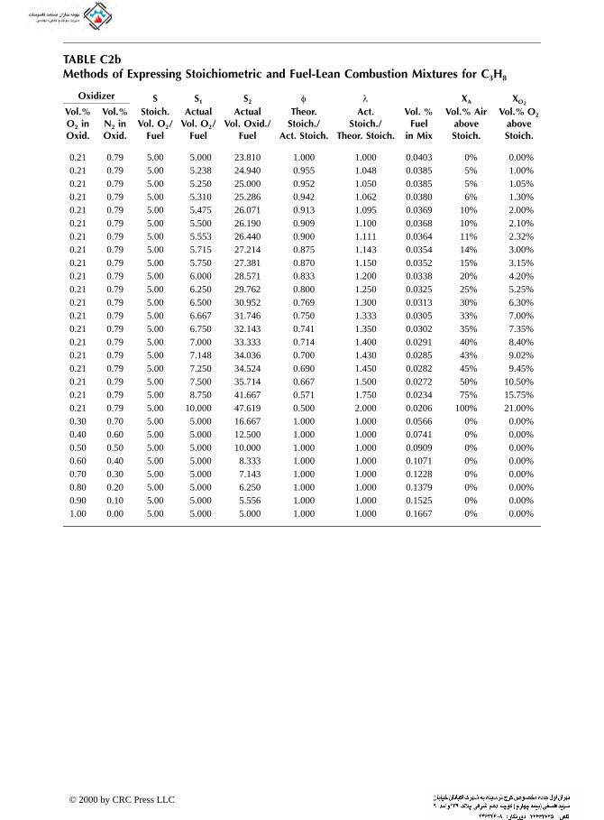
TABLE C2b
Methods of Expressing Stoichiometric and Fuel-Lean Combustion Mixtures for C3H8
Oxidizer S S1 S2 φ λ XA XO2
Vol.% O2 in Oxid.
Vol.% N2 in Oxid.
Stoich. Vol. O2 /
Fuel
Actual Vol. O2 /
Fuel
Actual Vol. Oxid./
Fuel
Theor. Stoich./
Act. Stoich.
Act. Stoich./
Theor. Stoich.
Vol. % Fuel
in Mix
Vol.% Air above Stoich.
Vol.% O2 above Stoich.
0.21 0.79 5.00 5.000 23.810 1.000 1.000 0.0403 0% 0.00%0.21 0.79 5.00 5.238 24.940 0.955 1.048 0.0385 5% 1.00%0.21 0.79 5.00 5.250 25.000 0.952 1.050 0.0385 5% 1.05%0.21 0.79 5.00 5.310 25.286 0.942 1.062 0.0380 6% 1.30%0.21 0.79 5.00 5.475 26.071 0.913 1.095 0.0369 10% 2.00%0.21 0.79 5.00 5.500 26.190 0.909 1.100 0.0368 10% 2.10%0.21 0.79 5.00 5.553 26.440 0.900 1.111 0.0364 11% 2.32%0.21 0.79 5.00 5.715 27.214 0.875 1.143 0.0354 14% 3.00%0.21 0.79 5.00 5.750 27.381 0.870 1.150 0.0352 15% 3.15%0.21 0.79 5.00 6.000 28.571 0.833 1.200 0.0338 20% 4.20%0.21 0.79 5.00 6.250 29.762 0.800 1.250 0.0325 25% 5.25%0.21 0.79 5.00 6.500 30.952 0.769 1.300 0.0313 30% 6.30%0.21 0.79 5.00 6.667 31.746 0.750 1.333 0.0305 33% 7.00%0.21 0.79 5.00 6.750 32.143 0.741 1.350 0.0302 35% 7.35%0.21 0.79 5.00 7.000 33.333 0.714 1.400 0.0291 40% 8.40%0.21 0.79 5.00 7.148 34.036 0.700 1.430 0.0285 43% 9.02%0.21 0.79 5.00 7.250 34.524 0.690 1.450 0.0282 45% 9.45%0.21 0.79 5.00 7.500 35.714 0.667 1.500 0.0272 50% 10.50%0.21 0.79 5.00 8.750 41.667 0.571 1.750 0.0234 75% 15.75%0.21 0.79 5.00 10.000 47.619 0.500 2.000 0.0206 100% 21.00%0.30 0.70 5.00 5.000 16.667 1.000 1.000 0.0566 0% 0.00%0.40 0.60 5.00 5.000 12.500 1.000 1.000 0.0741 0% 0.00%0.50 0.50 5.00 5.000 10.000 1.000 1.000 0.0909 0% 0.00%0.60 0.40 5.00 5.000 8.333 1.000 1.000 0.1071 0% 0.00%0.70 0.30 5.00 5.000 7.143 1.000 1.000 0.1228 0% 0.00%0.80 0.20 5.00 5.000 6.250 1.000 1.000 0.1379 0% 0.00%0.90 0.10 5.00 5.000 5.556 1.000 1.000 0.1525 0% 0.00%1.00 0.00 5.00 5.000 5.000 1.000 1.000 0.1667 0% 0.00%
© 2000 by CRC Press LLC

TABLE C3a
Methods of Expressing Fuel-Rich Combustion Mixtures for H2
Oxidizer S S1 S2 φ λ XA XO2
Vol.% O2 in Oxid.
Vol.% N2 in Oxid.
Stoich. Vol. O2 /
Fuel
Actual Vol. O2 /
Fuel
Actual Vol. Oxid./
Fuel
Theor. Stoich./
Act. Stoich.
Act. Stoich./
Theor. Stoich.
Vol. % Fuel
in Mix
Vol.% Air above Stoich.
Vol.% O2 above Stoich.
0.21 0.79 0.50 0.125 0.595 4.000 0.250 0.6269 –75% –15.75%0.21 0.79 0.50 0.250 1.190 2.000 0.500 0.4565 –50% –10.50%0.21 0.79 0.50 0.263 1.253 1.900 0.526 0.4439 – 47% –9.95%0.21 0.79 0.50 0.275 1.310 1.818 0.550 0.4330 – 45% –9.45%0.21 0.79 0.50 0.278 1.323 1.800 0.556 0.4305 – 44% –9.33%0.21 0.79 0.50 0.294 1.401 1.700 0.588 0.4166 – 41% –8.65%0.21 0.79 0.50 0.300 1.429 1.667 0.600 0.4118 – 40% –8.40%0.21 0.79 0.50 0.313 1.488 1.600 0.625 0.4019 –38% –7.88%0.21 0.79 0.50 0.325 1.548 1.538 0.650 0.3925 –35% –7.35%0.21 0.79 0.50 0.333 1.587 1.500 0.667 0.3865 –33% –7.00%0.21 0.79 0.50 0.350 1.667 1.429 0.700 0.3750 –30% –6.30%0.21 0.79 0.50 0.357 1.701 1.400 0.715 0.3702 –29% –6.00%0.21 0.79 0.50 0.375 1.786 1.333 0.750 0.3590 –25% –5.25%0.21 0.79 0.50 0.385 1.831 1.300 0.769 0.3532 –23% – 4.85%0.21 0.79 0.50 0.400 1.905 1.250 0.800 0.3443 –20% – 4.20%0.21 0.79 0.50 0.417 1.984 1.200 0.833 0.3351 –17% –3.50%0.21 0.79 0.50 0.425 2.024 1.176 0.850 0.3307 –15% –3.15%0.21 0.79 0.50 0.450 2.143 1.111 0.900 0.3182 –10% –2.10%0.21 0.79 0.50 0.455 2.164 1.100 0.909 0.3160 –9% –1.91%0.21 0.79 0.50 0.472 2.249 1.059 0.945 0.3078 –6% –1.17%0.21 0.79 0.50 0.475 2.262 1.053 0.950 0.3066 –5% –1.05%
© 2000 by CRC Press LLC

TABLE C3b
Methods of Expressing Stoichiometric and Fuel-Lean Combustion Mixtures for H2
Oxidizer S S1 S2 φ λ XA XO2
Vol.% O2 in Oxid.
Vol.% N2 in Oxid.
Stoich. Vol. O2 /
Fuel
Actual Vol. O2 /
Fuel
Actual Vol. Oxid./
Fuel
Theor. Stoich./
Act. Stoich.
Act. Stoich./
Theor. Stoich.
Vol. % Fuel
in Mix
Vol.% Air above Stoich.
Vol.% O2 above Stoich.
0.21 0.79 0.50 0.500 2.381 1.000 1.000 0.2958 0% 0.00%0.21 0.79 0.50 0.524 2.494 0.955 1.048 0.2862 5% 1.00%0.21 0.79 0.50 0.525 2.500 0.952 1.050 0.2857 5% 1.05%0.21 0.79 0.50 0.531 2.529 0.942 1.062 0.2834 6% 1.30%0.21 0.79 0.50 0.548 2.607 0.913 1.095 0.2772 10% 2.00%0.21 0.79 0.50 0.550 2.619 0.909 1.100 0.2763 10% 2.10%0.21 0.79 0.50 0.555 2.644 0.900 1.111 0.2744 11% 2.32%0.21 0.79 0.50 0.572 2.721 0.875 1.143 0.2687 14% 3.00%0.21 0.79 0.50 0.575 2.738 0.870 1.150 0.2675 15% 3.15%0.21 0.79 0.50 0.600 2.857 0.833 1.200 0.2593 20% 4.20%0.21 0.79 0.50 0.625 2.976 0.800 1.250 0.2515 25% 5.25%0.21 0.79 0.50 0.650 3.095 0.769 1.300 0.2442 30% 6.30%0.21 0.79 0.50 0.667 3.175 0.750 1.333 0.2395 33% 7.00%0.21 0.79 0.50 0.675 3.214 0.741 1.350 0.2373 35% 7.35%0.21 0.79 0.50 0.700 3.333 0.714 1.400 0.2308 40% 8.40%0.21 0.79 0.50 0.715 3.404 0.700 1.430 0.2271 43% 9.02%0.21 0.79 0.50 0.725 3.452 0.690 1.450 0.2246 45% 9.45%0.21 0.79 0.50 0.750 3.571 0.667 1.500 0.2188 50% 10.50%0.21 0.79 0.50 0.875 4.167 0.571 1.750 0.1935 75% 15.75%0.21 0.79 0.50 1.000 4.762 0.500 2.000 0.1736 100% 21.00%0.30 0.70 0.50 0.500 1.667 1.000 1.000 0.3750 0% 0.00%0.40 0.60 0.50 0.500 1.250 1.000 1.000 0.4444 0% 0.00%0.50 0.50 0.50 0.500 1.000 1.000 1.000 0.5000 0% 0.00%0.60 0.40 0.50 0.500 0.833 1.000 1.000 0.5455 0% 0.00%0.70 0.30 0.50 0.500 0.714 1.000 1.000 0.5833 0% 0.00%0.80 0.20 0.50 0.500 0.625 1.000 1.000 0.6154 0% 0.00%0.90 0.10 0.50 0.500 0.556 1.000 1.000 0.6429 0% 0.00%1.00 0.00 0.50 0.500 0.500 1.000 1.000 0.6667 0% 0.00%
© 2000 by CRC Press LLC

Appendix D
Properties for CH4, C3H8, and H2 Flames
© 2000 by CRC Press LLC

ition Oxidizer (298K) (Metric Units)
ition Oxidizer (77°F) (English Units)
TABLE D1aH2 (298K) Adiabatically and Stoichiometrically (φ = 1.00) Combusted with a Variable-Compos
TABLE D1bH2 (77°F) Adiabatically and Stoichiometrically (φ = 1.00) Combusted with a Variable-Compos
© 2000 by CRC Press LLC

TABLE D2aH2 (298K) Adiabatically ir (Variable Temp.) (Metric Units)
© 2000 by CRC Press LL
and Stoichiometrically (φ = 1.00) Combusted with A
C
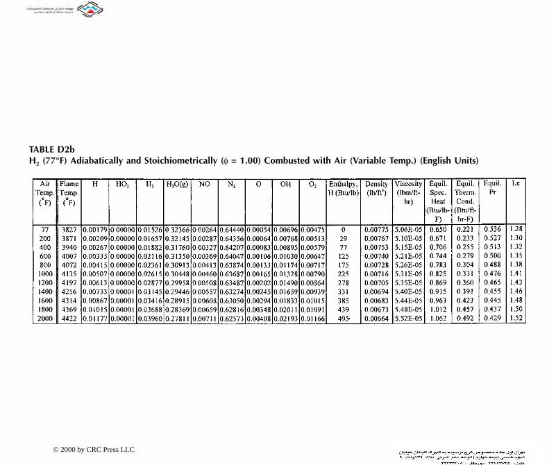
TABLE D2bH2 (77°F) Adiabatically ir (Variable Temp.) (English Units)
© 2000 by CRC Press LL
and Stoichiometrically (φ = 1.00) Combusted with A
C

etric Units)
TAH ish Units)
TABLE D3aH2 (Variable Temp.) Adiabatically and Stoichiometrically (φ = 1.00) Combusted with Air (298K) (M
BLE D3b2 (Variable Temp.) Adiabatically and Stoichiometrically (φ = 1.00) Combusted with Air (77°F) (Engl
© 2000 by CRC Press LLC

TABLE D4aH2 (298K) Stoich
© 2000 by CR
iometrically (φ = 1.00) Combusted with Air (298K) (Metric Units)
C Press LLC

TABLE D4bH2 (Variable Tem Air (77°F) (English Units)
© 2000 by CR
p.) Adiabatically and Stoichiometrically (φ = 1.00) Combusted with
C Press LLC

TABLEH2 (29 )
TABLEH2 (77
D5a8K) Adiabatically Combusted with Air (298K) at Various Equivalence Ratios (Metric Units
D5b°F) Combusted with Air (77°F) at Various Equivalence Ratios (English Units)
© 2000 by CRC Press LLC

TABLE D6aH2 (298K) Stoichiometr .) with an Exhaust Temp. of 1367K (Metric Units)
© 2000 by CRC Press L
ically (φ = 1.00) Combusted with Air (Variable Temp
LC

TABLE D6bH2 (77°F) Stoichiometri ith an Exhaust Temp. of 2000°F (English Units)
© 2000 by CRC Press L
cally (φ = 1.00) Combusted with Air (Variable Temp.) w
LC

TACH Oxidizer (298K) (Metric Units)
TABCH Oxidizer (77°F) (English Units)
BLE D7a4 (298K) Adiabatically and Stoichiometrically (φ = 1.00) Combusted with a Variable Composition
LE D7b4 (77°F) Adiabatically and Stoichiometrically (φ = 1.00) Combusted with a Variable Composition
© 2000 by CRC Press LLC

TABLE D8aCH4 (298K) Adiabatically Air (Variable Temp.) (Metric Units)
© 2000 by CRC Press LL
and Stoichiometrically (φ = 1.00) Combusted with
C

TABLE D8bCH4 (77°F) Adiabatically ir (Variable Temp.) (English Units)
© 2000 by CRC Press L
and Stoichiometrically (φ = 1.00) Combusted with A
LC

TC etric Units)
TACH lish Units)
ABLE D9aH4 (Variable Temp.) Adiabatically and Stoichiometrically (φ = 1.00) Combusted with Air (298K) (M
BLE D9b4 (Variable Temp.) Adiabatically and Stoichiometrically (φ = 1.00) Combusted with Air (77°F) (Eng
© 2000 by CRC Press LLC

TABLE D10aCH4 (298K) Stoich
© 2000 by CRC
iometrically (φ = 1.00) Combusted with Air (298K) (Metric Units)
Press LLC

TABLE D10bCH4 (Variable Temp ith Air (77°F) (English Units)
© 2000 by CRC
.) Adiabatically and Stoichiometrically (φ = 1.00) Combusted w
Press LLC

TABLE DCH4 (29 its)
TABLE DCH4 (77
Equiv.
Ratio
FlaTe
(K
lpy,/kg)
Density
(kg/m3)
Viscosity(kg/m-s)
Equil.Spec.Heat
(kJ/kg-K)
Equil.Therm.Cond.(W/m-
K)
Equil.Pr
Le
4.00 9 4 0.246 3.85E-05 6.71 0.401 0.644 0.802.00 15 8 0.177 5.55E-05 1.66 0.152 0.603 0.991.33 20 7 0.154 6.68E-05 1.61 0.168 0.640 1.061.00 22 8 0.150 7.12E-05 2.19 0.248 0.630 1.120.80 19 8 0.170 6.65E-05 1.59 0.151 0.698 1.030.67 17 5 0.192 6.18E-05 1.44 0.123 0.723 1.000.57 16 1 0.213 5.79E-05 1.38 0.110 0.726 1.000.50 14 3 0.233 5.48E-05 1.33 0.100 0.729 1.00
Equiv.
Ratio
FlaTe
(°
th-py,Btub)
Density(lb/ft3)
Viscosity(lbm/ft-hr)
Equil.Spec.Heat
(Btu/lb-
°F)
Equil.Therm.Cond.(Btu/ft-hr-F)
Equil.Pr
Le
4.00 12 80 0.01537 2.59E-05 1.602 0.232 0.644 0.802.00 23 10 0.01105 3.73E-05 0.395 0.088 0.603 0.991.33 31 45 0.00963 4.49E-05 0.385 0.097 0.640 1.061.00 35 11 0.00938 4.79E-05 0.524 0.143 0.630 1.120.80 31 0 0.01061 4.47E-05 0.379 0.087 0.698 1.030.67 27 5 0.01196 4.16E-05 0.344 0.071 0.723 1.000.57 24 5 0.01328 3.90E-05 0.330 0.064 0.726 1.000.50 22 7 0.01452 3.68E-05 0.319 0.058 0.729 1.00
©
11a8K) Adiabatically Combusted with Air (298K) at Various Equivalence Ratios (Metric Un
11b°F) Combusted with Air (77°F) at Various Equivalence Ratios (English Units)
memp.
)
C(gr) CH4 CO CO2 H H2 H2O(g) NH3 NO N2 O OH O2 EnthaH (kJ
44 0.0483 0.02281 0.11559 0.02752 0.00000 0.33907 0.04363 0.00012 0.00000 0.40293 0.00000 0.00000 0.00000 -8863 0.0000 0.00000 0.11939 0.02850 0.00002 0.17637 0.11939 0.00000 0.00000 0.55633 0.00000 0.00000 0.00000 -4830 0.0000 0.00000 0.06524 0.05041 0.00044 0.05021 0.18077 0.00000 0.00002 0.65273 0.00000 0.00017 0.00000 -3325 0.0000 0.00000 0.00893 0.08539 0.00039 0.00361 0.18338 0.00000 0.00197 0.70866 0.00021 0.00291 0.00455 -2595 0.0000 0.00000 0.00050 0.07692 0.00002 0.00022 0.15380 0.00000 0.00323 0.72654 0.00012 0.00164 0.03699 -2081 0.0000 0.00000 0.00004 0.06540 0.00000 0.00002 0.13059 0.00000 0.00223 0.73705 0.00003 0.00053 0.06411 -1712 0.0000 0.00000 0.00000 0.05656 0.00000 0.00000 0.11304 0.00000 0.00135 0.74460 0.00000 0.00017 0.08427 -1578 0.0000 0.00000 0.00000 0.04988 0.00000 0.00000 0.09973 0.00000 0.00080 0.75018 0.00000 0.00005 0.09934 -13
memp.
F)
C(gr) CH4 CO CO2 H H2 H2O(g) NH3 NO N2 O OH O2 Enal
H(/l
40 0.0483 0.02281 0.11559 0.02752 0.00000 0.33907 0.04363 0.00012 0.00000 0.40293 0.00000 0.00000 0.00000 -353 0.0000 0.00000 0.11939 0.02850 0.00002 0.17637 0.11939 0.00000 0.00000 0.55633 0.00000 0.00000 0.00000 -295 0.0000 0.00000 0.06524 0.05041 0.00044 0.05021 0.18077 0.00000 0.00002 0.65273 0.00000 0.00017 0.00000 -145 0.0000 0.00000 0.00893 0.08539 0.00039 0.00361 0.18338 0.00000 0.00197 0.70866 0.00021 0.00291 0.00455 -132 0.0000 0.00000 0.00050 0.07692 0.00002 0.00022 0.15380 0.00000 0.00323 0.72654 0.00012 0.00164 0.03699 -947 0.0000 0.00000 0.00004 0.06540 0.00000 0.00002 0.13059 0.00000 0.00223 0.73705 0.00003 0.00053 0.06411 -741 0.0000 0.00000 0.00000 0.05656 0.00000 0.00000 0.11304 0.00000 0.00135 0.74460 0.00000 0.00017 0.08427 -601 0.0000 0.00000 0.00000 0.04988 0.00000 0.00000 0.09973 0.00000 0.00080 0.75018 0.00000 0.00005 0.09934 -5
2000 by CRC Press LLC

TABLE D12aCH4 (298K) Stoichiometr ) with an Exhaust Temp. of 1367K (Metric Units)
© 2000 by CRC Press L
ically (φ = 1.00) Combusted with Air (Variable Temp.
LC

TABLE D12bCH4 (77°F) Stoichiomet with an Exhaust Temp. of 2000°F (English Units)
© 2000 by CRC Press
rically (φ = 1.00) Combusted with Air (Variable Temp.)
LLC

TAC3 Oxidizer (298K) (Metric Units)
TAC3 Oxidizer (77°F) (English Units)
BLE D13aH8 (298K) Adiabatically and Stoichiometrically (φ = 1.00) Combusted with a Variable-Composition
BLE D13bH8 (77°F) Adiabatically and Stoichiometrically (φ = 1.00) Combusted with a Variable-Composition
© 2000 by CRC Press LLC

TABLE D14aC3H8 (298K) Adiabatica Air (Variable Temp.) (Metric Units)
© 2000 by CRC Press L
lly and Stoichiometrically (φ = 1.00) Combusted with
LC

TABLE D14bC3H8 (77°F) Adiabaticall ir (Variable Temp.) (English Units)
© 2000 by CRC Press L
y and Stoichiometrically (φ = 1.00) Combusted with A
LC

TABLE D15aC3H8 (Variable Temp.) Ad usted with Air (298K) (Metric Units)
© 2000 by CRC Press LLC
iabatically and Stoichiometrically (φ = 1.00) Comb

TABLE D15bC3H8 (Variable Temp.) Ad ted with Air (77°F) (English Units)
© 2000 by CRC Press L
iabatically and Stoichiometrically (φ = 1.00) Combus
LC

TABLE D16aC3H8 (298K) Stoic )
© 2000 by CRC
hiometrically (φ = 1.00) Combusted with Air (298K) (Metric Units
Press LLC

TABLE D16bC3H8 (Variable T ith Air (77°F) (English Units)
© 2000 by CR
emp.) Adiabatically and Stoichiometrically (φ = 1.00) Combusted w
C Press LLC

TABLC3H8 nits)
TABLC3H8
E D17a (298K) Adiabatically Combusted with Air (298K) at Various Equivalence Ratios (Metric U
E D17b (77°F) Combusted with Air (77°F) at Various Equivalence Ratios (English Units)
© 2000 by CRC Press LLC

TABLE D18aC3H8 (298K) Stoichiom p.) with an Exhaust Temp. of 1367K (Metric Units)
© 2000 by CRC Press L
etrically (φ = 1.00) Combusted with Air (Variable Tem
LC

TABLE D18bC3H8 (77°F) Stoichiometric with an Exhaust Temp. of 2000°F (English Units)
© 2000 by CRC Press LL
ally (φ = 1.00) Combusted with Air (Variable Temp.)
C

TABLE D19aH2 + CH4 (298K) Stoichio etric Units)
© 2000 by CRC Press L
metrically (φ = 1.00) Combusted with Air (298K) (M
LC

TABLE D19bH2 + CH4 (298K) Stoichio lish Units)
© 2000 by CRC Press L
metrically (φ = 1.00) Combusted with Air (77°F) (Eng
LC
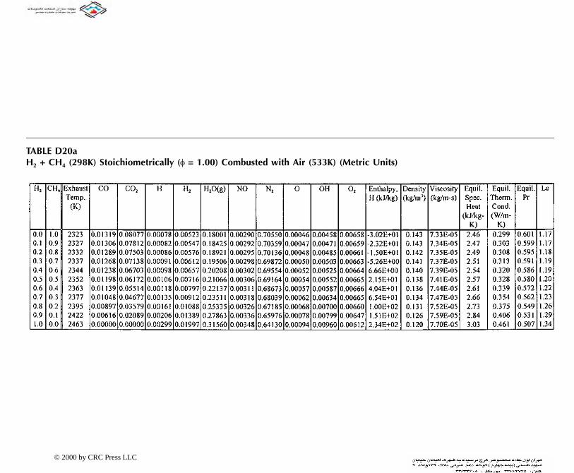
TABLE D20aH2 + CH4 (298K) Stoichi etric Units)
© 2000 by CRC Press L
ometrically (φ = 1.00) Combusted with Air (533K) (M
LC

TABLE D20bH2 + CH4 (298K) Stoichio nglish Units)
© 2000 by CRC Press LL
metrically (φ = 1.00) Combusted with Air (500°F) (E
C
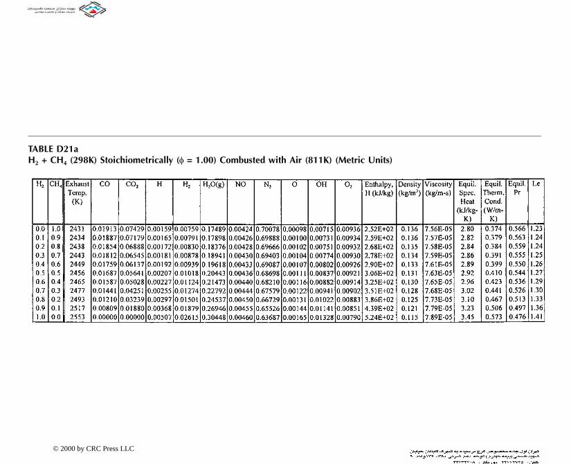
TABLE D21aH2 + CH4 (298K) Stoich etric Units)
© 2000 by CRC Press L
iometrically (φ = 1.00) Combusted with Air (811K) (M
LC
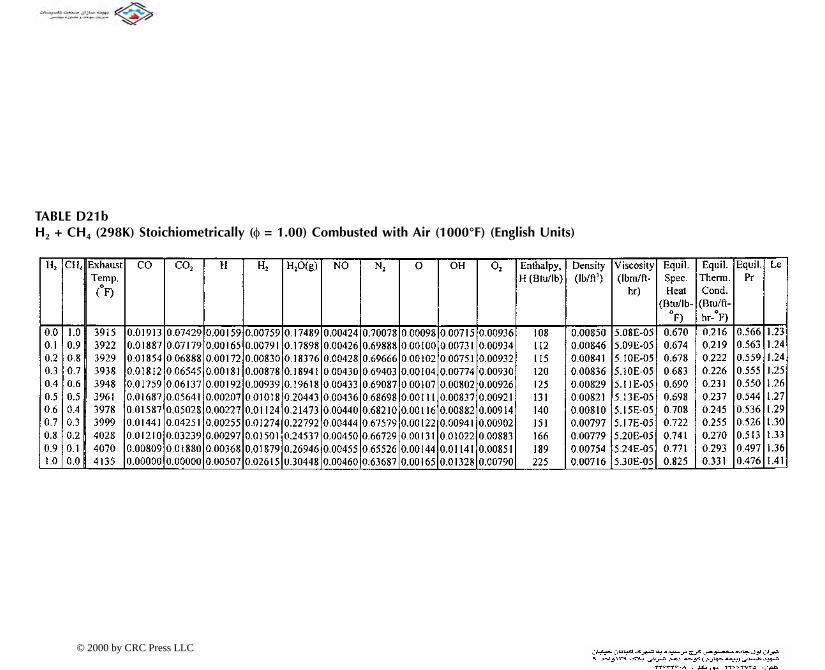
TABLE D21bH2 + CH4 (298K) Stoichio (English Units)
© 2000 by CRC Press LL
metrically (φ = 1.00) Combusted with Air (1000°F)
C

TABLE D22aH2 + CH4 (298K) Stoichi (Metric Units)
© 2000 by CRC Press LL
ometrically (φ = 1.00) Combusted with Air (1089K)
C

TABLE D22bH2 + CH4 (298K) Stoich glish Units)
© 2000 by CRC Press
iometrically (φ = 1.00) Combusted with Air (1500°F) (En
ß
LLC

Appendix E
Fluid Dynamics Equations
E.1 FLUID DYNAMICS EQUATIONS IN CYLINDRICAL COORDINATES
The unsteady equations of motion for an incompressible Newtonian fluid with constant viscosity in cylindrical coordinates (r,θ,z) are given as follows:
(E.1)
(E.2)
(E.3)
where fi is some type of body force such as buoyancy. The energy equation for an incompressible fluid can be written as:
(E.4)
where
∂∂
+ ∂∂
+ ∂∂
− + ∂∂
=
− ∂∂
+ ∂∂
∂( )∂
⎡
⎣⎢⎢
⎤
⎦⎥⎥
+ ∂∂
−∂∂
+ ∂∂
⎧⎨⎪
⎩⎪
⎫⎬⎪
⎭⎪
vv
v
r
v
r
v v
rw
v
z
fpr
vr r
rv
r r
v
r
v v
z
rr
r r r
rr r r
τ θ
ρ θ θ
θ θ
θ
2
2
2
2 2
2
2
1 1 1 2
∂∂
+∂∂
+∂∂
+ +∂∂
=
− ∂∂
+ ∂∂
∂( )∂
⎡
⎣⎢⎢
⎤
⎦⎥⎥
+∂∂
+ ∂∂
+∂∂
⎧⎨⎪
⎩⎪
⎫⎬⎪
⎭⎪
vv
v
r
v
r
v v v
rw
v
z
fr
pv
r r
rv
r r
v
r
v v
z
rr
r
θ θ θ θ θ θ
θθ θ θ
τ θ
ρ θ θ θ1 1 1 2
2
2
2 2
2
2
∂∂
+ ∂∂
+ ∂∂
+ ∂∂
= − ∂∂
+ ∂∂
∂∂
⎛⎝⎜
⎞⎠⎟ + ∂
∂+ ∂
∂⎧⎨⎩
⎫⎬⎭
wv
wr
v
rw
wwz
fpz
vr r
rwr r
w wzr zτ θ ρ θ
θ 1 1 12
2
2
2
2
ρτ θ θ θ
θct
vtr
v
rt
wtz r r
rktr r
kt
zk
tz
qp r
∂∂
+ ∂∂
+ ∂∂
+ ∂∂
⎛⎝⎜
⎞⎠⎟ = ∂
∂∂∂
⎛⎝⎜
⎞⎠⎟ + ∂
∂∂∂
⎛⎝⎜
⎞⎠⎟ + ∂
∂∂∂
⎛⎝⎜
⎞⎠⎟ + +1 1
2˙ Φ
© 2000 by CRC Press LLC

∂⎛
⎜⎞⎟ +
∂+⎛
⎜⎞⎟
⎡⎢
⎤⎥ + ∂⎛⎜ ⎞⎟ +
∂+ ∂⎛
⎜⎞⎟
1 1 12 2 2 2
v vv
w v wrr
θ θ⎧⎪
⎫⎪
(E.5)
E.2 FLUID DYNAMICS EQUATIONS IN SPHERICAL COORDINATES
The unsteady equations of motion for an incompressible Newtonian fluid with constant viscosity in spherical coordinates (r,θ,φ) are given as follows:
(E.6)
(E.7)
(E.8)
where fi is some type of body force such as buoyancy and
The energy equation for an incompressible fluid can be written as:
(E.9)
Φ = µ∂⎝ ⎠ ∂⎝ ⎠⎣ ⎦ ∂⎝ ⎠ ∂ ∂⎝ ⎠
+ ∂∂
+ ∂∂
⎛⎝⎜
⎞⎠⎟
+ ∂∂
+ ∂∂
⎛⎝
⎞⎠
⎡2
2
12
12
12
r r z z r
wr
v
z r
vr
r
v
rr r θ
θ θ
θ⎣⎣⎢⎤⎦⎥
⎨⎪⎪
⎩
⎪⎪⎪
⎬⎪⎪
⎭
⎪⎪⎪
2
∂∂
+ ∂∂
+ ∂∂
+ ∂∂
−+
=
− ∂∂
+ ∇ − −∂∂
− −∂∂
⎧⎨⎩
⎫⎬⎭
vv
v
r
v
r
v v
r
v v v
r
fpr
v fv
r r
v
rv
r
v
rr
r r r
r rr
τ θ θ φ
ρ θθ
θ φ
θ φ θ φ
θθ
φ
sin
cotsin
2 2
22 2 2 2
1 2 2 2 2
∂∂
+∂∂
+∂∂
+∂∂
+ − =
− ∂∂
+ ∇ + ∂∂
− −∂∂
⎧⎨⎩
⎫⎬⎭
vv
v
r
v
r
v v
r
v v v
r
v
r
fr
pv v
r
v v
r r
v
rr
r
θ θ θ θ φ θ θ φ
θ θθ φ
τ θ θ φθ
ρ θ θ θθθ φ
sin
cot
sincossin
2
22 2 2 2 2
1 2 2
∂∂
+∂∂
+∂∂
+∂∂
+ − =
− ∂∂
+ ∇ − + ∂∂
+∂∂
⎧⎨⎩
⎫⎬⎭
vv
v
r
v
r
v v
r
v v v
r
v v
r
fr
pv v
v
r r
v
r
v
rr
r
φ φ θ φ φ φ φ θ φ
φ φφ θ
τ θ θ φθ
ρ θ φ θ θ φθθ φ
sin
cot
sin sin sincossin
1 2 222 2 2 2 2
∇ ≡ ∂∂
∂∂
⎛⎝⎜
⎞⎠⎟ + ∂
∂∂
∂⎛⎝⎜
⎞⎠⎟ + ∂
∂2
22
2 2 2
2
2
1 1 1r r
rr r rsin
sinsinθ θ
θθ θ φ
ρτ θ θ φ
θ θθ
θ θ φ φ
θ φct
vtr
v
rt v
rt
r rr k
tr
rk
tr
kt
q
p r
∂∂
+ ∂∂
+ ∂∂
+ ∂∂
⎛⎝⎜
⎞⎠⎟
= ∂∂
∂∂
⎛⎝⎜
⎞⎠⎟
+ ∂∂
∂∂
⎛⎝⎜
⎞⎠⎟ + ∂
∂∂∂
⎛⎝⎜
⎞⎠⎟
+ +
sin
sinsin
sin˙
1
1 1
22
2 2 2 Φ
© 2000 by CRC Press LLC

where
(E.10)Φ = µ
∂∂
⎛⎝⎜
⎞⎠⎟
+∂∂
+⎛⎝⎜
⎞⎠⎟
⎡
⎣⎢
⎤
⎦⎥
+∂∂
+ +⎛⎝⎜
⎞⎠⎟
+ ∂∂
⎛⎝⎜
⎞⎠⎟
+∂∂
⎡
⎣⎢
⎤
⎦⎥
+∂∂
+ ∂∂
2
1
1 1 12
1
12
1
2 2
2
2 2
v
r r
vv
r
vv v r
r
v
r r
v
r
vr
r
v
rr
rr
r
θ
φθ
θ
φ
θ
θ φθ
θ
θ φ
sincot
sin rr r
v
r
v⎛⎝⎜
⎞⎠⎟
⎡
⎣⎢
⎤
⎦⎥ + ∂
∂⎛⎝⎜
⎞⎠⎟
+∂∂
⎡
⎣⎢
⎤
⎦⎥
⎧
⎨
⎪⎪⎪⎪⎪
⎩
⎪⎪⎪⎪⎪
⎫
⎬
⎪⎪⎪⎪⎪
⎭
⎪⎪⎪⎪⎪
2 212
1sinsin sin
θθ θ θ φ
φ θ
© 2000 by CRC Press LLC

Appendix F
Material Properties
TABLE F.1aProperties of Air (English Units)
T (°F)
ρ(lb/ft3)
cp
(Btu/lb-°F)µ
(lbm/hr-ft)k
(Btu/hr-ft-°F) Pr
–9 0.08707 0.2403 0.0386 0.0129 0.72081 0.07251 0.2405 0.0447 0.0152 0.707
171 0.06212 0.2410 0.0504 0.0173 0.700261 0.05438 0.2422 0.0557 0.0195 0.690351 0.04832 0.2439 0.0607 0.0216 0.686441 0.04348 0.2460 0.0654 0.0235 0.684531 0.03951 0.2484 0.0698 0.0254 0.683621 0.03623 0.2510 0.0740 0.0271 0.685711 0.03344 0.2539 0.0781 0.0287 0.690801 0.03106 0.2567 0.0820 0.0303 0.695891 0.02899 0.2596 0.0859 0.0317 0.702981 0.02718 0.2625 0.0895 0.0331 0.709
1071 0.02558 0.2651 0.0931 0.0344 0.7161161 0.02415 0.2677 0.0964 0.0358 0.7201251 0.02289 0.2701 0.0996 0.0372 0.7231341 0.02174 0.2725 0.1028 0.0385 0.7261521 0.01977 0.2768 0.1087 0.0413 0.7281701 0.01812 0.2806 0.1145 0.0441 0.7281881 0.01673 0.2840 0.1201 0.0474 0.7192061 0.01553 0.2883 0.1283 0.0526 0.7032241 0.01450 0.2938 0.1349 0.0578 0.685
Source: From F. Kreith, Ed., The CRC Handbook of Mechanical Engineering,
CRC Press, Boca Raton, FL, 1998, A-32–A-33.
© 2000 by CRC Press LLC

TABLE F.1b
Properties of Air (Metric Units)
T ρ cp η × 107 λ × 103
(K) (kg/m3) [kJ/(kg · K)] ](N · s)/m2] [W/(m · K)] Pr
100 3.5562 1.032 71.1 9.34 0.786150 2.3364 1.012 103.4 13.8 0.758200 1.7458 1.007 132.5 18.1 0.737250 1.3947 1.006 159.6 22.3 0.720300 1.1614 1.007 184.6 26.3 0.707350 0.9950 1.009 208.2 30.0 0.700400 0.8711 1.014 230.1 33.8 0.690450 0.7740 1.021 250.7 37.3 0.686500 0.6964 1.030 270.1 40.7 0.684550 0.6329 1.040 288.4 43.9 0.683600 0.5804 1.051 305.8 46.9 0.685650 0.5356 1.063 322.5 49.7 0.690700 0.4975 1.075 338.8 52.4 0.695750 0.4643 1.087 354.6 54.9 0.702800 0.4354 1.099 369.8 57.3 0.709850 0.4097 1.110 384.3 59.6 0.716900 0.3868 1.121 398.1 62.0 0.720950 0.3666 1.131 411.3 64.3 0.723
1000 0.3482 1.141 424.4 66.7 0.7261100 0.3166 1.159 449.0 71.5 0.7281200 0.2902 1.175 473.0 76.3 0.7281300 0.2679 1.189 496.0 82 0.7191400 0.2488 1.207 530 91 0.7031500 0.2322 1.230 557 100 0.685
Source: From G.F. Hewitt, G.L. Shires, and T.R. Bott, Eds., Process Heat
Transfer, CRC Press, Boca Raton, FL, 1994, 1018.
© 2000 by CRC Press LLC

TABLE F.2
Gas Properties
© 2000 by CRC Press LLC

TABLE F.2 (continued)
Gas Properties
© 2000 by CRC Press LLC

TABLE F.2 (continued)
Gas Properties
© 2000 by CRC Press LLC

TABLE F.2 (continued)
Gas Properties
© 2000 by CRC Press LLC

TABLE F.2 (continued)
Gas Properties
© 2000 by CRC Press LLC
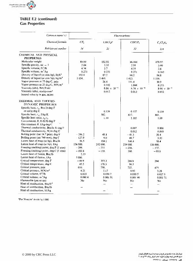
TABLE F.2 (continued)
Gas Properties
© 2000 by CRC Press LLC

TABLE F.2 (continued)
Gas Properties
© 2000 by CRC Press LLC

TABLE F.2 (continued)
Gas Properties
© 2000 by CRC Press LLC

TABLE F.2 (continued)
Gas Properties
© 2000 by CRC Press LLC
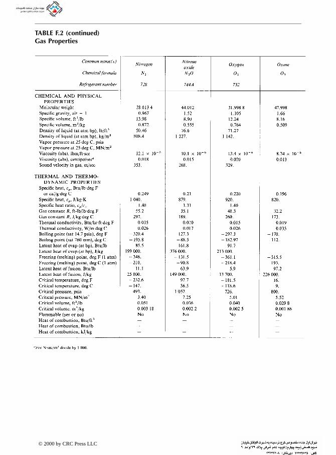
TABLE F.2 (continued)
Gas Properties
© 2000 by CRC Press LLC

TABLE F.2 (continued)
Gas Properties
© 2000 by CRC Press LLC

TABLE F.2 (continued)
Source: From F. Kreith, Ed., The CRC Handbook of Mechanical Engineering, CRC Press, Boca Raton, FL, 1998, A-18–A-29.
Gas Properties
© 2000 by CRC Press LLC

TP
C
perties at Various Temperatures (K)
λ [W/(m · K)]/cp[J/(kg · K)]
600 800 1000 1200 1500 2000 2500
A 231 218
1033 1146 186 1042 185 —B 126 106 90.8 78.7
2604 2823 3018 3227 3519B
B 10.6 9.60 9.851892 2160 2338
C
C 80.7 71.3 65.4 61.9 57.2 49.4542 581 616 682 779 937
C 67.4 58.2 52.1 49.3 42.5503 550 628 733 674
C 379 366 352 339
417 433 451 480 59 545 74 — 149 425
ABLE F.3 roperties of Metals
omposition
MeltingPoint(K)
Properties at 300 K Pro
ρ cp λ κ × 106
(kg/m3) [J/(kg · K)] [W/(m · K)] (m2/sec) 100 200 400
luminumPure 933 2702 903 237 97.1 302 237 240
482 798 949Alloy 2024-T6 775 2770 875 177 73.0 65 163 186 (4.5% Cu, 1.5% Mg, 0.6% Mn) 473 787 925Alloy 195, cast 2790 883 168 68.2 174 (4.5% Cu) —
eryllium 1550 1850 1825 200 59.2 990 301 161203 1114 2191
ismuth 545 9780 122 7.86 6.59 16.5 9.69 7.04112 120 127
oron 2573 2500 1107 27.0 9.76 190 55.5 16.8128 600 1463
admium 594 8650 231 96.8 48.4 203 99.3 94.7198 222 242
hromium 2118 7160 449 93.7 29.1 159 111 90.9192 384 484
obalt 1769 8862 421 99.2 26.6 167 122 85.4236 379 450
opperPure 1358 8933 385 401 117 482 413 393
252 356 397Commercial bronze 1293 8800 420 52 14 42 52 (90% Cu, 10% Al) 785 460Phosphor gear bronze 1104 8780 355 54 17 41 65 (89% Cu, 11% Sn) — —Cartridge brass 1188 8530 380 110 33.9 75 95 137 (70% Cu, 30% Zn) 360 395
© 2000 by CRC Press LLC

C Ger 27.3 19.8 17.4 17.4
348 357 375 395Gol 298 284 270 255
135 140 145 155Irid 138 132 126 120 111
138 144 153 161 172Iron P 54.7 43.3 32.8 28.3 32.1
574 680 975 609 654 A 53.1 42.2 32.3 28.7 31.4
574 680 975 609 654Car P 48.0 39.2 30.0 559 685 1169 A 48.8 39.2 31.3
559 685 1168 C 44.0 37.4 29.3 582 699 971 C 39.7 35.0 27.6
559 685 1090
Chr C 36.7 33.3 26.9
575 688 969
TAPro
Com
operties at Various Temperatures (K)
λ [W/(m · K)]/cp[J/(kg · K)]
600 800 1000 1200 1500 2000 2500
onstantan 1493 8920 384 23 6.71 17 19(55% Cu, 45% Ni) 237 362manium 1211 5360 322 59.9 34.7 232 96.8 43.2
190 290 337d 1336 19,300 129 317 127 327 323 311
109 124 131ium 2720 22,500 130 147 50.3 172 153 144
90 122 133
ure 1810 7870 447 80.2 23.1 134 94.0 69.5216 384 490
rmco 7870 447 72.7 20.7 95.6 80.6 65.7215 384 490
bon steelslain carbon 7854 434 60.5 17.7 56.7(Mn ð 1%, Si ð 0.1%) 487ISI 1010 7832 434 63.9 18.8 58.7
487arbon-silicon 7817 446 51.9 14.9 49.8(Mn ð 1%, 0.1% < Si ð 0.6%) 501arbon-manganese-silicon 8131 434 41.0 11.6 42.2(1% < Mn ð 1.6%, 0.1% < Si ð 0.6%)
487
omium (low) steelsr- Mo-Si 7822 444 37.7 10.9 38.2
(0.18% C, 0.65% Cr, 0.23% Mo, 0.6% Si)
492
BLE F.3 (continued) perties of Metals
position
MeltingPoint(K)
Properties at 300 K Pr
ρ cp λ κ × 106
(kg/m3) [J/(kg · K)] [W/(m · K)] (m2/sec) 100 200 400
© 2000 by CRC Press LLC

1 39.1 34.5 27.4
575 688 969
1 42.1 36.3 28.2 575 688 969Stai A 20.0 22.8 25.4
559 585 606 A 19.8 22.6 25.4 28.0 31.7
557 582 611 640 682 A 18.3 21.3 24.2
18.3 21.3 24.2 A 18.9 21.9 24.7
559 585 606Lea 31.4
142Ma 149 146
1170 1267Mo 126 118 112 105 98 90 86
275 285 295 308 330 380 459Nic P 65.6 67.6 71.8 76.2 82.6
592 530 562 594 616 N 16 21 525 545 I 17.0 20.5 24.0 27.6 33.0 510 546 626 — —
TAPro
Com
operties at Various Temperatures (K)
λ [W/(m · K)]/cp[J/(kg · K)]
600 800 1000 1200 1500 2000 2500
Cr- Mo 7858 442 42.3 12.2 42.0(0.16% C, 1% Cr, 0.54% Mo, 0.39% Si)
492
Cr-V 7836 443 48.9 14.1 46.8(0.2% C, 1.02% Cr, 0.15% V) 492nless steelsISI 302 8055 480 15.1 3.91 17.3
512ISI 304 1670 7900 477 14.9 3.95 9.2 12.6 16.6
272 402 515ISI 316 8238 468 13.4 3.48 15.2
15.2ISI 347 7978 480 14.2 3.71 15.8
513d 601 11,340 129 35.3 24.1 39.7 36.7 34.0
118 125 132gnesium 923 1740 1024 156 87.6 169 159 153
649 934 1074lybdenum 2894 10,240 251 138 53.7 179 143 134
141 224 261kelure 1728 8900 444 90.7 23.0 164 107 80.2
232 383 485ichrome 1672 8400 420 12 3.4 14(80% Ni, 20% Cr) 480nconel X-750 1665 8510 439 11.7 3.1 8.7 10.3 13.5(73% Ni, 15% Cr, 6.7% Fe) 372 473
BLE F.3 (continued) perties of Metals
position
MeltingPoint(K)
Properties at 300 K Pr
ρ cp λ κ × 106
(kg/m3) [J/(kg · K)] [W/(m · K)] (m2/sec) 100 200 400
© 2000 by CRC Press LLC

Nio 58.2 61.3 64.4 67.5 72.1 79.1283 292 301 310 324 347
Pall 79.7 86.9 94.2 102 110261 271 281 291 307
Plat P 73.2 75.6 78.7 82.6 89.5 99.4
141 146 152 157 165 179 A 59 65 69 73 76 — — — — —Rhe 44.2 44.1 44.6 45.7 47.8 51.9
145 151 156 162 171 186Rho 136 127 121 116 110 112
274 293 311 327 349 376Sili 61.9 42.2 31.2 25.7 22.7
867 913 946 967 992Silv 412 396 379 361
250 262 277 292Tan 58.6 59.4 60.2 61.0 62.2 64.1 65.6
146 149 152 155 160 172 189Tho 55.8 56.9 56.9 58.7
134 145 156 167Tin
Tita 19.4 19.7 20.7 22.0 24.5633 675 620 686
Tun 137 125 118 113 107 100 95142 145 148 152 157 167 176
TAPro
Com
operties at Various Temperatures (K)
λ [W/(m · K)]/cp[J/(kg · K)]
600 800 1000 1200 1500 2000 2500
bium 2741 8570 265 53.7 23.6 55.2 52.6 55.2188 249 274
adium 1827 12,020 244 71.8 24.5 76.5 71.6 73.6168 227 251
inumure 2045 21,450 133 71.6 25.1 77.5 72.6 71.8
100 125 136lloy 60Pt-40Rh 1800 16,630 162 47 17.4 52(60% Pt, 40% Rh) —nium 3453 21,100 136 47.9 16.7 58.9 51.0 46.1
97 127 139dium 2236 12,450 243 150 49.6 186 154 146
147 220 253con 1685 2330 712 148 89.2 884 264 98.9
259 556 790er 1235 10,500 235 429 174 444 430 425
187 225 239talum 3269 16,600 140 57.5 24.7 59.2 57.5 57.8
110 133 144rium 2023 11,700 118 54.0 39.1 59.8 54.6 54.5
99 112 124505 7310 227 66.6 40.1 85.2 73.3 62.2
188 215 243nium 1953 4500 522 21.9 9.32 30.5 24.5 20.4
300 465 551 591gsten 3660 19,300 132 174 68.3 208 186 159
87 122 137
BLE F.3 (continued) perties of Metals
position
MeltingPoint(K)
Properties at 300 K Pr
ρ cp λ κ × 106
(kg/m3) [J/(kg · K)] [W/(m · K)] (m2/sec) 100 200 400
© 2000 by CRC Press LLC

U 34.0 38.8 43.9 49.0146 176 180 161
Va 33.3 35.7 38.2 40.8 44.6 50.9540 563 597 645 714 867
Zi 103436
Zi 20.7 21.6 23.7 26.0 28.8 33.0322 342 362 344 344 344
So 5.
TAP
Co
perties at Various Temperatures (K)
λ [W/(m · K)]/cp[J/(kg · K)]
600 800 1000 1200 1500 2000 2500
ranium 1406 19,070 116 27.6 12.5 21.7 25.1 29.694 108 125
nadium 2192 6100 489 30.7 10.3 35.8 31.3 31.3258 430 515
nc 693 7140 389 116 41.8 117 118 111297 367 402
cronium 2125 6570 278 22.7 12.4 33.2 25.2 21.6205 264 300
urce: From G.F. Hewitt, G.L. Shires, and T.R. Bott, Eds., Process Heat Transfer, CRC Press, Boca Raton, FL, 1994, 1022-102
BLE F.3 (continued) roperties of Metals
mposition
MeltingPoint(K)
Properties at 300 K Pro
ρ cp λ κ × 106
(kg/m3) [J/(kg · K)] [W/(m · K)] (m2/sec) 100 200 400
© 2000 by CRC Press LLC