HEAT TRANSFER ENHANCEMENT DUE TO SURFACE OXIDATION...
117
1 HEAT TRANSFER ENHANCEMENT DUE TO SURFACE OXIDATION OF METHANE ON PLATINUM By SUNGSIK KIM A THESIS PRESENTED TO THE GRADUATE SCHOOL OF THE UNIVERSITY OF FLORIDA IN PARTIAL FULFILLMENT OF THE REQUIREMENTS FOR THE DEGREE OF MASTER OF SCIENCE UNIVERSITY OF FLORIDA 2011
Transcript of HEAT TRANSFER ENHANCEMENT DUE TO SURFACE OXIDATION...
1
HEAT TRANSFER ENHANCEMENT DUE TO SURFACE OXIDATION OF METHANE ON PLATINUM
By
SUNGSIK KIM
A THESIS PRESENTED TO THE GRADUATE SCHOOL OF THE UNIVERSITY OF FLORIDA IN PARTIAL FULFILLMENT
OF THE REQUIREMENTS FOR THE DEGREE OF MASTER OF SCIENCE
UNIVERSITY OF FLORIDA
2011

2
© 2011 Sungsik Kim

3
To my family
4
ACKNOWLEDGMENTS
I thank my parents to support me to study at University of Florida and sister to
help me. Moreover, I thank my friend, Gobong to recommend me this school. And, I
thank my advisor, Dr. David W. Mikolaitis to give me a chance to research methane
under enhancement of heat transfer and to teach me numerical programs and chemical
kinetics program. Finally, I thank my advisor to lead me to catalytic combustion field.
5
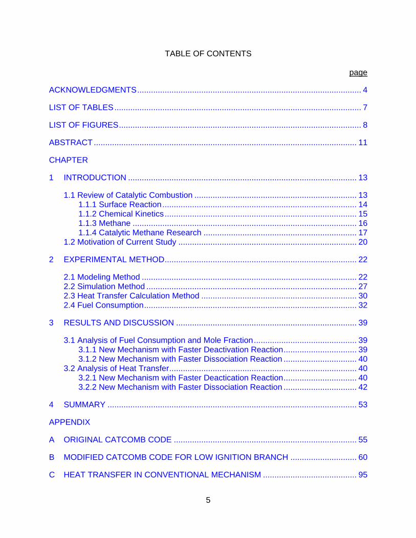
TABLE OF CONTENTS page
ACKNOWLEDGMENTS .................................................................................................. 4
LIST OF TABLES ............................................................................................................ 7
LIST OF FIGURES .......................................................................................................... 8
ABSTRACT ................................................................................................................... 11
CHAPTER
1 INTRODUCTION .................................................................................................... 13
1.1 Review of Catalytic Combustion ....................................................................... 13 1.1.1 Surface Reaction ..................................................................................... 14 1.1.2 Chemical Kinetics .................................................................................... 15 1.1.3 Methane .................................................................................................. 16 1.1.4 Catalytic Methane Research ................................................................... 17
1.2 Motivation of Current Study .............................................................................. 20
2 EXPERIMENTAL METHOD .................................................................................... 22
2.1 Modeling Method .............................................................................................. 22 2.2 Simulation Method ............................................................................................ 27 2.3 Heat Transfer Calculation Method .................................................................... 30 2.4 Fuel Consumption ............................................................................................. 32
3 RESULTS AND DISCUSSION ............................................................................... 39
3.1 Analysis of Fuel Consumption and Mole Fraction ............................................. 39 3.1.1 New Mechanism with Faster Deactivation Reaction ................................ 39 3.1.2 New Mechanism with Faster Dissociation Reaction ................................ 40
3.2 Analysis of Heat Transfer .................................................................................. 40 3.2.1 New Mechanism with Faster Deactication Reaction ................................ 40 3.2.2 New Mechanism with Faster Dissociation Reaction ................................ 42
4 SUMMARY ............................................................................................................. 53
APPENDIX
A ORIGINAL CATCOMB CODE ................................................................................ 55
B MODIFIED CATCOMB CODE FOR LOW IGNITION BRANCH ............................. 60
C HEAT TRANSFER IN CONVENTIONAL MECHANISM ......................................... 95
6
D HEAT TRANSFER IN NEW MECHANISM WITH FASTER DEACTIVATION ......... 96
E ENHANCEMENT OF HEAT TRANSFER IN NEW MECHANISM WITH FASTER DEACTIVATION ..................................................................................................... 97
F HEAT TRANSFER IN LOW IGNITION BRANCH IN NEW MECHANISM WITH FASTER DISSOCIATION ..................................................................................... 100
G HEAT TRANSFER IN HIGH IGNITION BRANCH IN NEW MECHANISM ............ 104
H ENHANCEMENT OF HEAT TRANSER ................................................................ 106
LIST OF REFERENCES ............................................................................................. 115
BIOGRAPHICAL SKETCH .......................................................................................... 117
7
LIST OF TABLES
Table page 2-1 Detailed surface mechanism of Deutschmann ................................................... 33
2-2 NASA coefficients of H2O ................................................................................... 33
2-3 NASA coefficients of H2O* .................................................................................. 34
2-4 NASA coefficients of CO2 ................................................................................... 34
2-5 NASA coefficients of CO2* .................................................................................. 34
2-6 Enthalpy of species at 700K.. ............................................................................. 34
2-7 Surface reactions in new mechanism ................................................................. 35
2-8 Gas reactions in new mechanism with faster deactivation reaction .................... 35
2-9 Gas reactions in new mechanism with the faster dissociation reaction .............. 36
8
LIST OF FIGURES
Figure page 1-1 Surface reaction process .................................................................................... 21
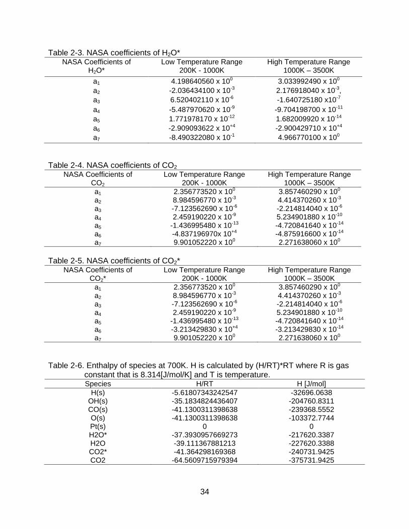
2-1 Reaction path of H(s) + OH(s) in Deutschmann mechanism. ............................. 36
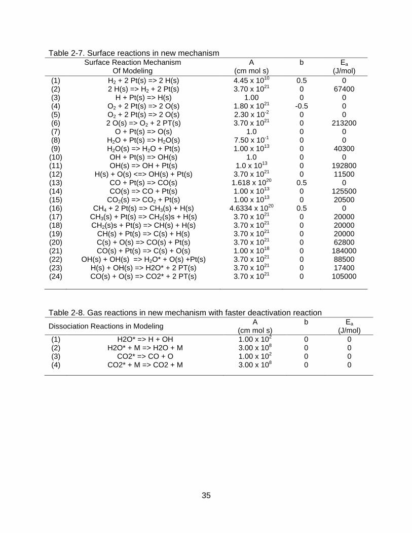
2-2 Reaction path of OH(s) + OH(s) and H2O(s) in Deutschmann mechanism. ....... 36
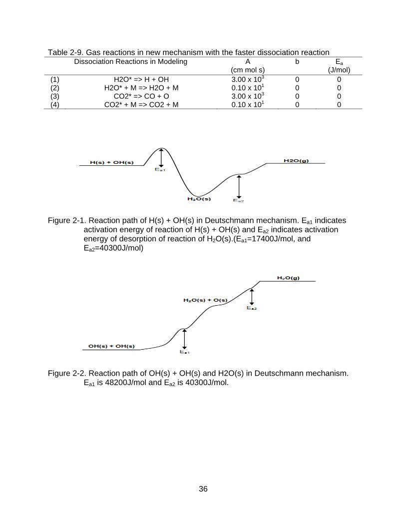
2-3 Reaction path of CO(s) + O(s) and CO2(s) in Deutschmann mechanism . ......... 37
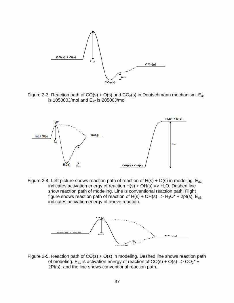
2-4 Reaction path of reaction of H(s) + O(s) in modeling. ......................................... 37
2-5 Reaction path of CO(s) + O(s) in modeling. ........................................................ 37
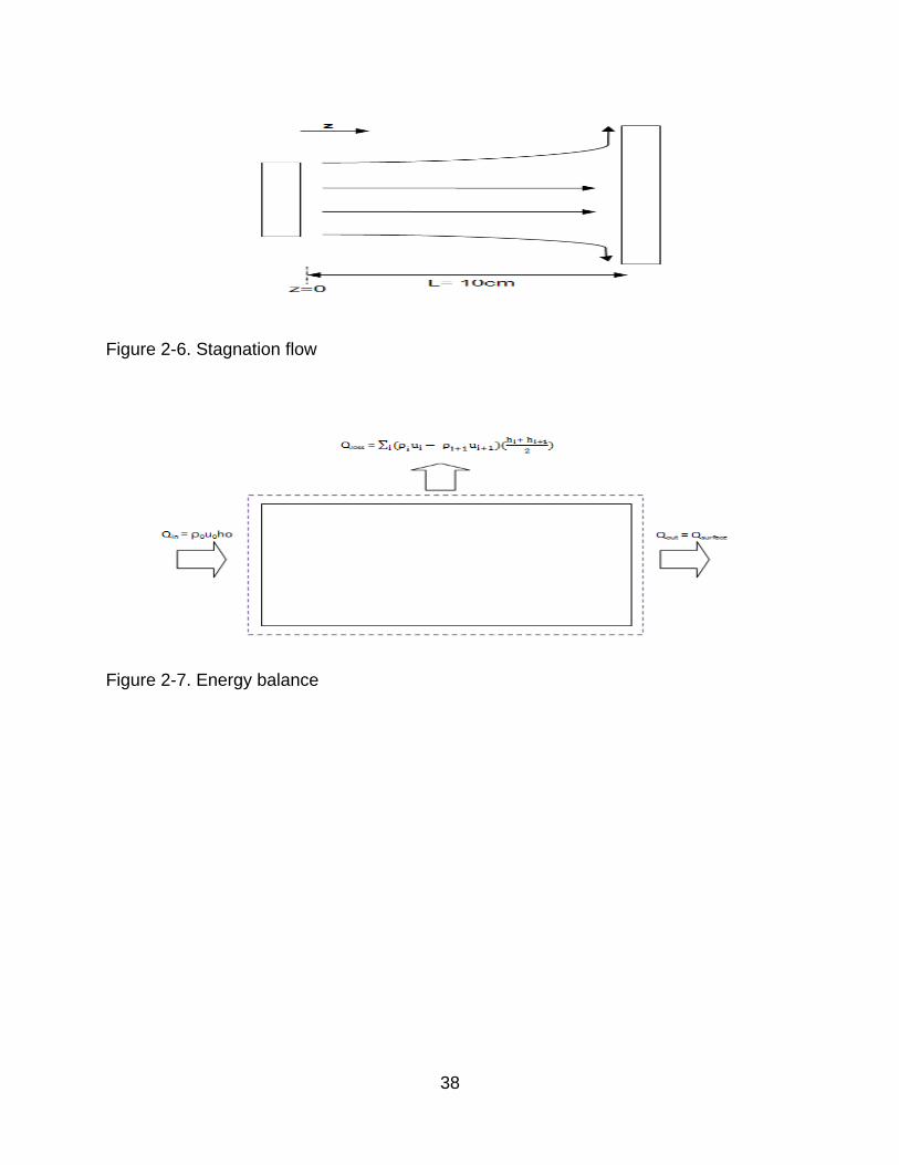
2-6 Stagnation flow ................................................................................................... 38
2-7 Energy balance ................................................................................................... 38
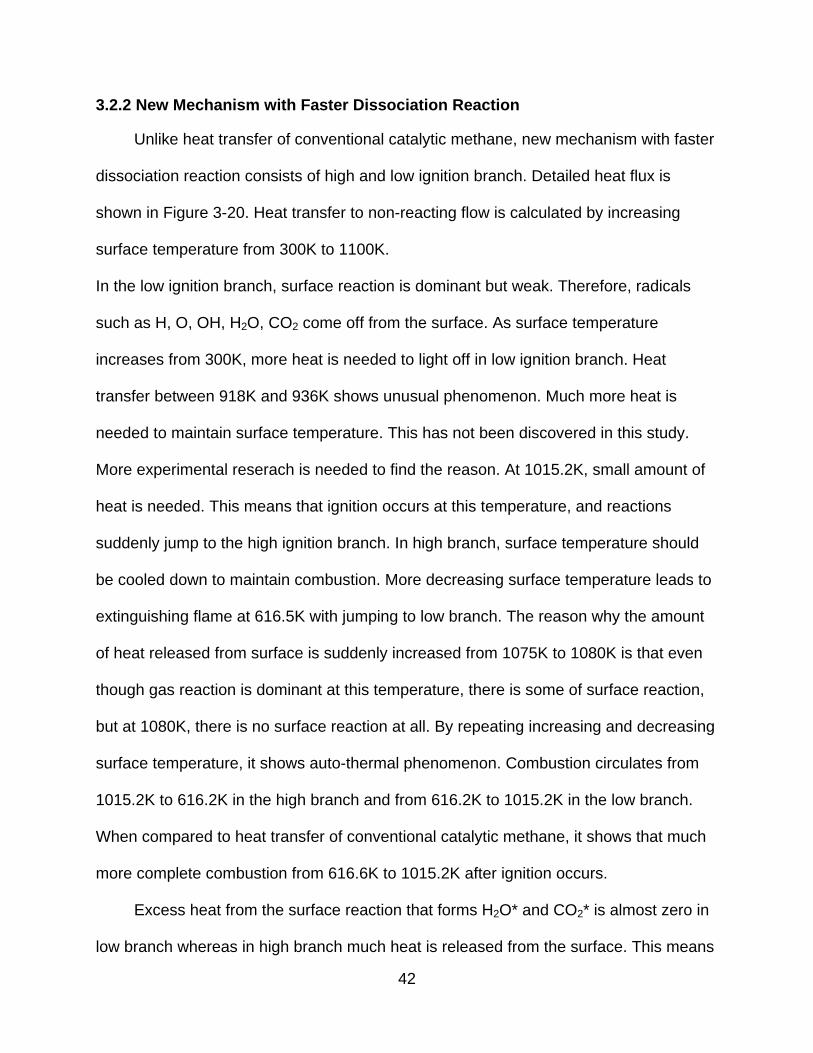
3-1 Mole fraction of species in Deutschmann at 900K .............................................. 44
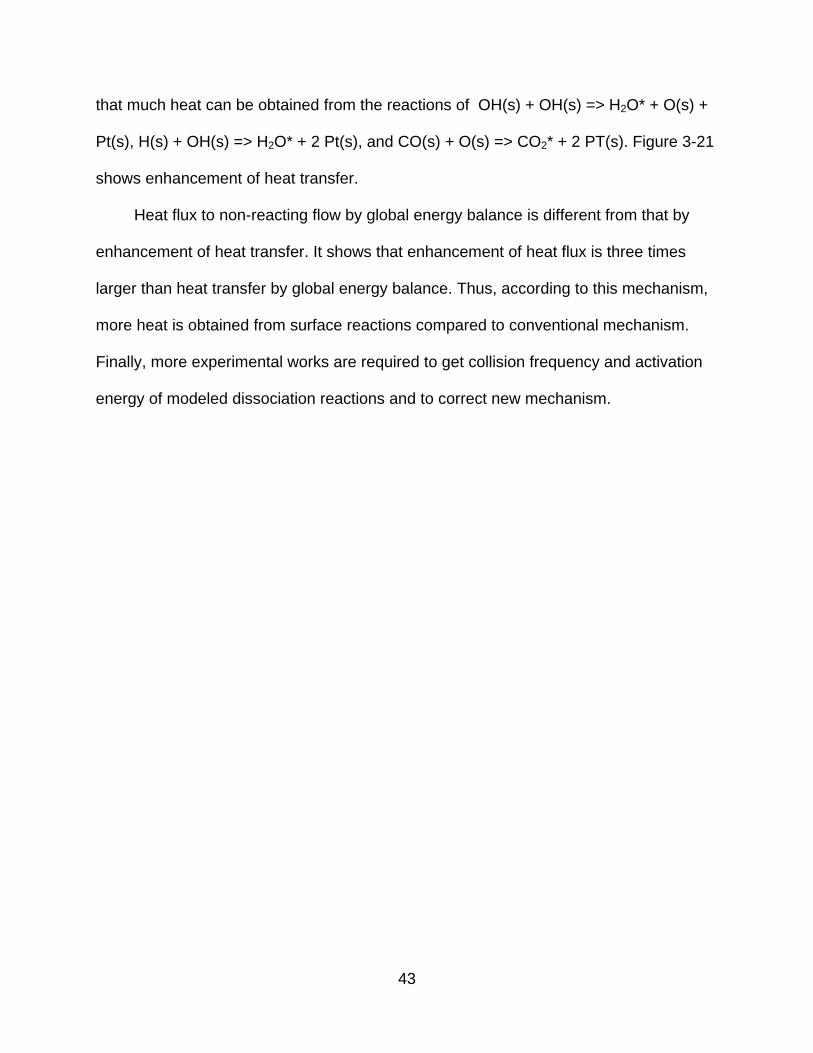
3-2 Axial velocity profile in Deutschmann at 900K .................................................... 44
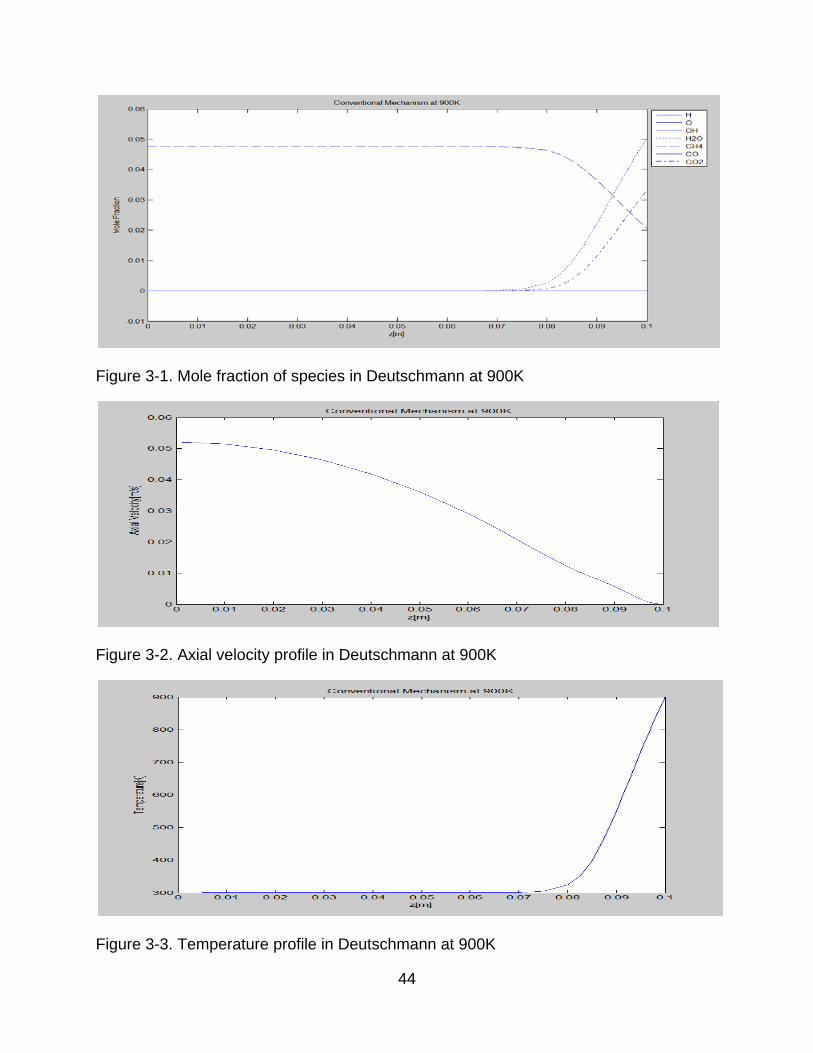
3-3 Temperature profile in Deutschmann at 900K .................................................... 44
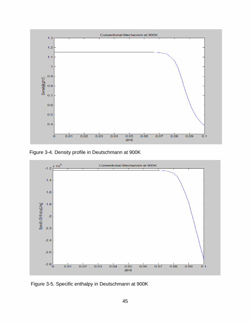
3-4 Density profile in Deutschmann at 900K ............................................................. 45
3-5 Specific enthalpy in Deutschmann at 900K ........................................................ 45
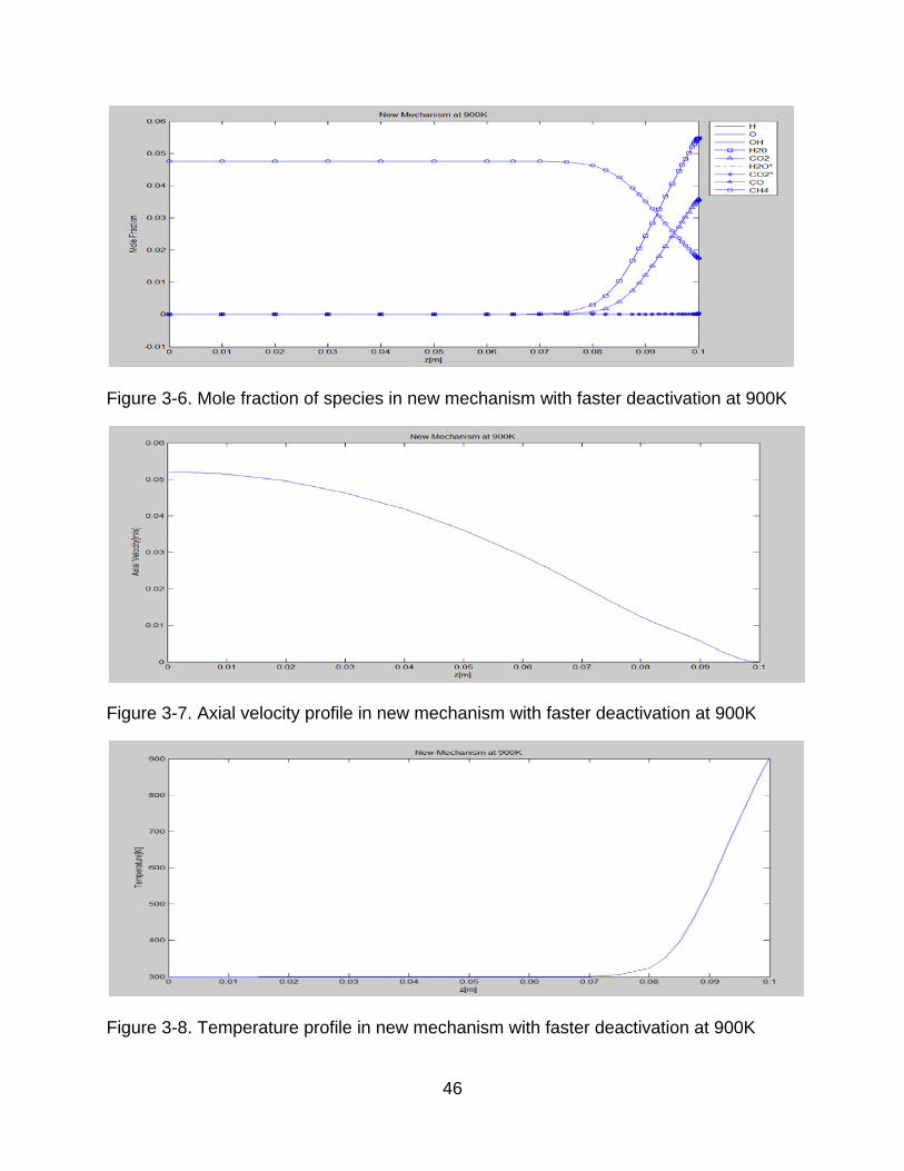
3-6 Mole fraction of species in new mechanism with faster deactivation at 900K ..... 46
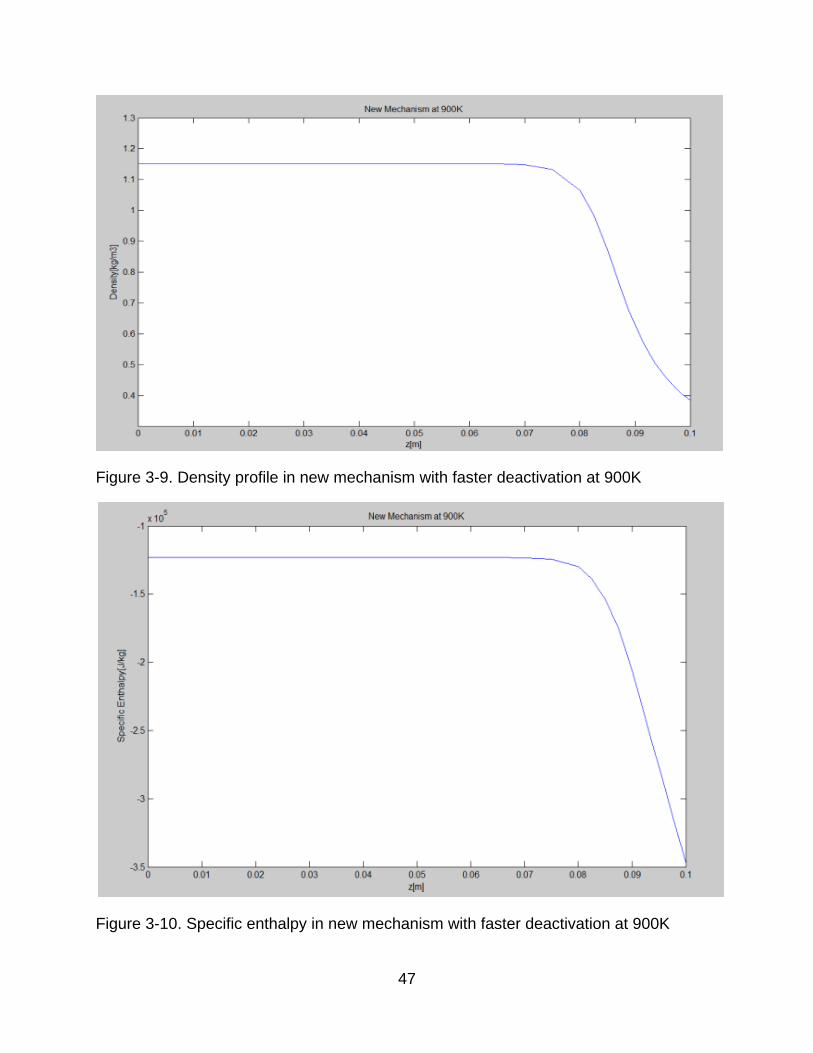
3-7 Axial velocity profile in new mechanism with faster deactivation at 900K ........... 46
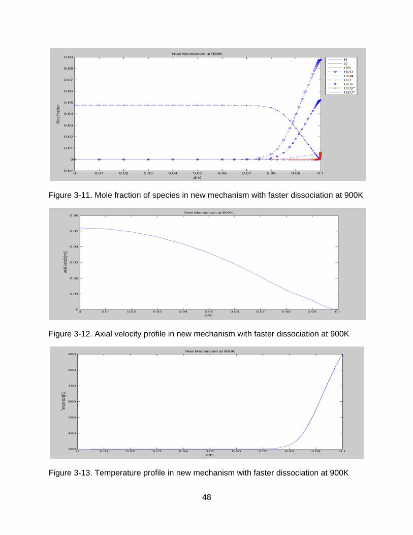
3-8 Temperature profile in new mechanism with faster deactivation at 900K ........... 46
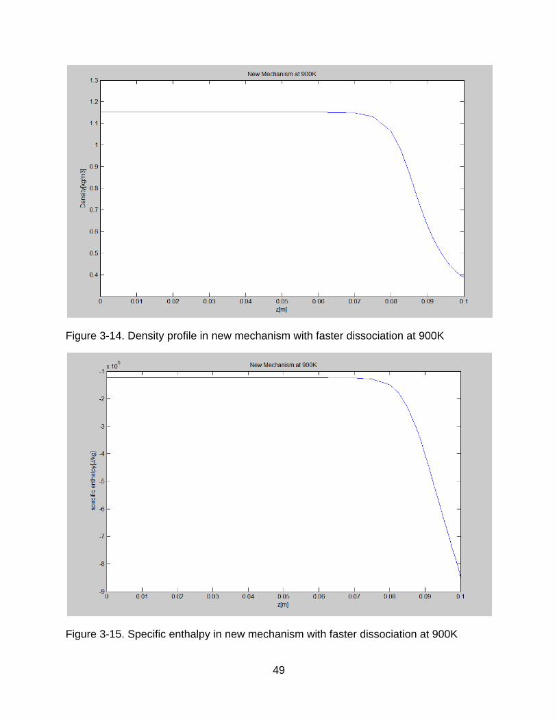
3-9 Density profile in new mechanism with faster deactivation at 900K .................... 47
3-10 Specific enthalpy in new mechanism with faster deactivation at 900K ............... 47
3-11 Mole fraction of species in new mechanism with faster dissociation at 900K ..... 48
3-12 Axial velocity profile in new mechanism with faster dissociation at 900K ........... 48
3-13 Temperature profile in new mechanism with faster dissociation at 900K ........... 48
3-14 Density profile in new mechanism with faster dissociation at 900K .................... 49
3-15 Specific enthalpy in new mechanism with faster dissociation at 900K ................ 49
9
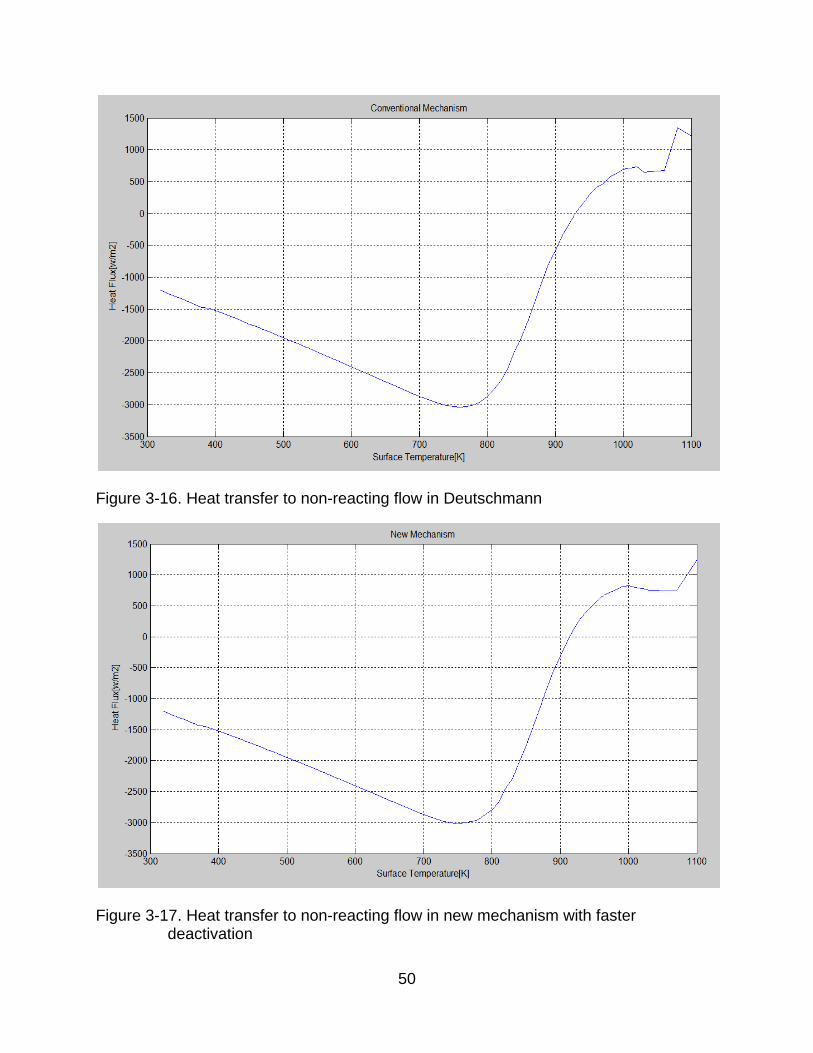
3-16 Heat transfer to non-reacting flow in Deutschmann ............................................ 50
3-17 Heat transfer to non-reacting flow in new mechanism with faster deactivation ... 50
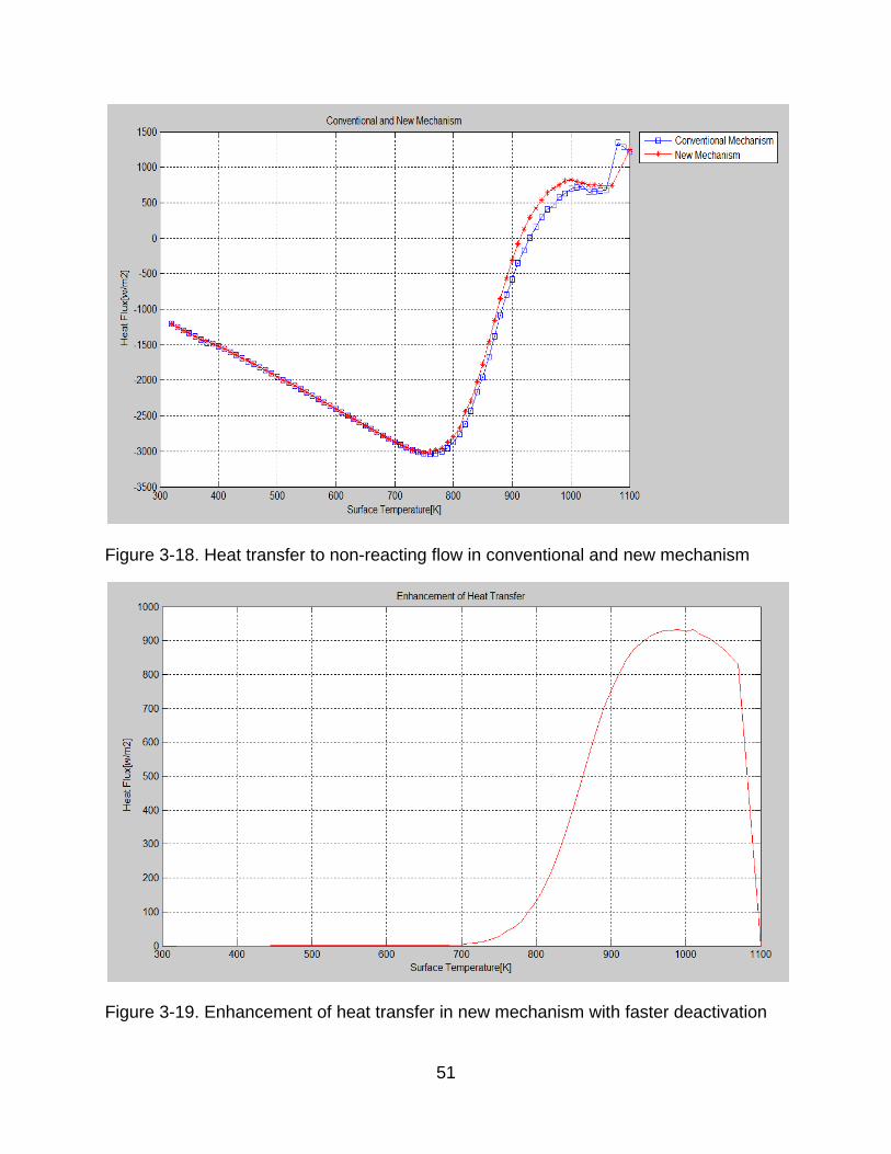
3-18 Heat transfer to non-reacting flow in conventional and new mechanism ............ 51
3-19 Enhancement of heat transfer in new mechanism with faster deactivation ........ 51
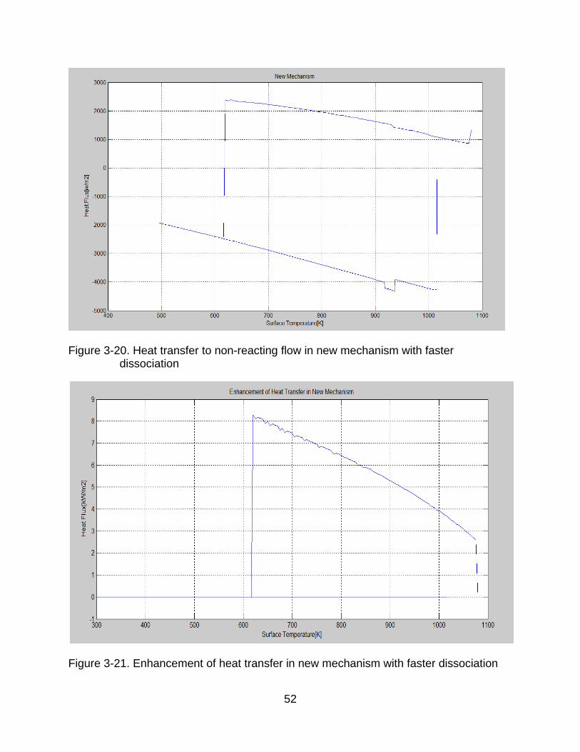
3-20 Heat transfer to non-reacting flow in new mechanism with faster dissociation ... 52
3-21 Enhancement of heat transfer in new mechanism with faster dissociation ......... 52
C-1 Heat flux to non-reacting flow in Deutschmann .................................................. 95
D-1 Heat flux to non-reacting flow in new mechanism with faster deactivation ......... 96
E-1 Heat flux to non-reacting flow from 320K to 560K in new mechanism with faster deactivation .............................................................................................. 97
E-2 Heat flux to non-reacting flow from 570K to 800K in new mechanism with faster deactivation .............................................................................................. 98
E-3 Heat flux to non-reacting flow from 820K to 1100K in new mechanism with faster deactivation .............................................................................................. 99
F-1 Heat flux to non-reacting flow from 320K to 605K in low ignition branch in new mechanism ................................................................................................ 100
F-2 Heat flux to non-reacting flow from 610K to 905K in low ignition branch in new mechanism ................................................................................................ 101
F-3 Heat flux to non-reacting flow from 910K to 1015.2K in low ignition branch in new mechanism ................................................................................................ 102
F-4 Heat flux to non-reacting flow from 916K to 937K in low ignition branch in new mechanism ................................................................................................ 103
G-1 Heat flux to non-reacting flow from 616.5K to910K in high ignition branch in new mechanism ................................................................................................ 104
G-2 Heat flux to non-reacting flow from 915K to 1080K in high ignition branch in new mechanism ................................................................................................ 105
H-1 Enhancement of heat transfer from 310K to 455K in low ignition branch in new mechanism ................................................................................................ 106
H-2 Enhancement of heat transfer from 460K to 605K in low ignition branch in new mechanism ................................................................................................ 107
10
H-3 Enhancement of heat transfer from 610K to 755K in low ignition branch in new mechanism ................................................................................................ 108
H-4 Enhancement of heat transfer from 610K to 905K in low ignition branch in new mechanism ................................................................................................ 109
H-5 Enhancement of heat transfer from 910K to 1015K in low ignition branch in new mechanism ................................................................................................ 110
H-6 Enhancement of heat transfer from 616.5K to 760K in high ignition branch in new mechanism ................................................................................................ 111
H-7 Enhancement of heat transfer from 765K to 910K in high ignition branch in new mechanism ................................................................................................ 112
H-8 Enhancement of heat transfer from 915K to 985K in high ignition branch in new mechanism ................................................................................................ 113
H-9 Enhancement of heat transfer from 990K to 1080K in high ignition branch in new mechanism ................................................................................................ 114
11
Abstract of Thesis Presented to the Graduate School of the University of Florida in Partial Fulfillment of the Requirements for the Degree of Master of Science
HEAT TRANSFER ENHANCEMENT DUE TO SURFACE OXIDATION OF METHANE
ON PLATINUM
By
Sungsik Kim
August 2011
Chair: Mikolaitis W, David Major: Mechanical Engineering
A study of methane is conducted on the conditions of premixed lean methane air
mixtures with platinum surface as a catalyst in one dimensional stagnation flow in
steady state to understand enhancement of heat transfer under a new surface
mechanism of methane oxidation. Premixed methane/air mixtures flowing onto platinum
surface of various surface temperatures are simulated. Enhancement of heat transfer
mechanism of catalytic methane oxidation is modeled based on GRI30 mechanism for
gas reactions and Deutschmann mechanism for surface reactions. In the proposed
surface mechanism, it is assumed that activated H2O and CO2 desorbs directly from
platinum surface without elementary surface reaction and that activated H2O and CO2
are dissociated or deactivated by third body reactions. Thus, three elementary surface
reactions are replaced in Deutschmann mechanism and four elementary reactions are
added in GRI30 mechanism. Deutschmann mechanism and new catalytic methane
mechanism are simulated and heat flux to non-reaction flow is calculated to see how
much heat is required to maintain a given surface temperature. By comparing to
conventional catalytic methane combustion, new mechanism shows different
phenomena in ignition temperature, fuel consumption at each surface temperature,
12
most importantly, heat transfer to non-reacting flow where there is no reactions due to
enhancement of heat transfer by adsorption and desorption. In addition, heat transfer to
non-reacting flow and enhancement of heat transfer are different with different rates of
dissociation and deactivation reactions. Because of insufficient information about heat
transfer to non-reacting flow, more research on enhancement of heat transfer is
required to prove this mechanism.
13
CHAPTER 1 INTRODUCTION
1.1 Review of Catalytic Combustion
Catalytic combustion becomes more an issue in that it reduces emission of NOx
because of lower operating temperature. Generally, it works by providing an alternative
mechanism involving a different transition state and lower activation energy. The
advantages of the catalytic combustion9 is that it does not require the presence of a
flame, nor an ignition source like a spark or pilot flame, but there is a minimum inlet gas
temperature required to have a sufficiently high catalyst activity to achieve complete
combustion. Second, it is operated at low temperature in which NOx would not be
formed. Thus, it is cleaner combustion process. Finally, it may enable the design of
more compact furnaces and reactors heated by combustion reactions to be
contemplated.
Catalytic combustion is a heterogeneous reaction that consists of two phase
reaction which is a gas-solid phase reaction. Surface reactions are important in many
combustion applications such as in wall recombination process during auto ignition, in
coal combustion, in soot formation and oxidation, in catalytic combustion or in metal
combustion. Rate of surface reaction varies with surface solid. It means that rate of
surface reaction can be significantly increased or decreased by the catalyst13 that is
substance attached to surface which affects rate of reaction without being consumed. If
catalyst speed the reaction, it is called positive catalysts whereas if it slows the reaction,
it is called inhibitors. And this phenomenon that rate of surface reaction is influenced by
catalyst is called catalysis.
14
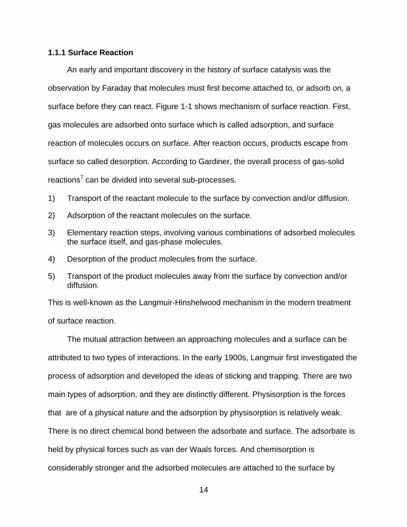
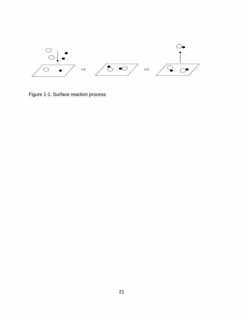
1.1.1 Surface Reaction
An early and important discovery in the history of surface catalysis was the
observation by Faraday that molecules must first become attached to, or adsorb on, a
surface before they can react. Figure 1-1 shows mechanism of surface reaction. First,
gas molecules are adsorbed onto surface which is called adsorption, and surface
reaction of molecules occurs on surface. After reaction occurs, products escape from
surface so called desorption. According to Gardiner, the overall process of gas-solid
reactions7 can be divided into several sub-processes.
1) Transport of the reactant molecule to the surface by convection and/or diffusion.
2) Adsorption of the reactant molecules on the surface.
3) Elementary reaction steps, involving various combinations of adsorbed molecules the surface itself, and gas-phase molecules.
4) Desorption of the product molecules from the surface.
5) Transport of the product molecules away from the surface by convection and/or diffusion.
This is well-known as the Langmuir-Hinshelwood mechanism in the modern treatment
of surface reaction.
The mutual attraction between an approaching molecules and a surface can be
attributed to two types of interactions. In the early 1900s, Langmuir first investigated the
process of adsorption and developed the ideas of sticking and trapping. There are two
main types of adsorption, and they are distinctly different. Physisorption is the forces
that are of a physical nature and the adsorption by physisorption is relatively weak.
There is no direct chemical bond between the adsorbate and surface. The adsorbate is
held by physical forces such as van der Waals forces. And chemisorption is
considerably stronger and the adsorbed molecules are attached to the surface by
15
valence forces of the same type as those occurring between bound atoms in molecules.
It occurs when the adsorbate and surface have a direct chemical bond causing the
sharing of electrons. The concept of chemisorptions was developed by Taylor7, Keier
and Roginsky7, Kummer and Emmett7, Constable7 and many others.
The Langmuir-Rideal mechanism7 or Rideal-Eley mechanism7 represents the
reaction between a gas molecule and an adsorbed molecule. In the precursor
mechanism7, species B is adsorbed on the metal catalyst surface, species A has just a
momentary residence on the surface without forming a bond on the surface, and the
reaction product AB is immediately formed.
In the desorption of product species, molecules requires sufficient energy to
overcome the bond strength between the adsorbed species and the surface. If the
desorption process of product species does not occur quickly at the catalytic surface,
product species can become saturated to stop the surface reaction process.
1.1.2 Chemical Kinetics
All chemical reactions have different rate of reaction under same conditions. It is
affected by concentrations the chemical compounds, temperature, pressure, presence
of a catalyst or inhibitor, and radiative effects. One-step chemical reaction of arbitrary
complexity can be represented by stoichiometric equation7.
� ν′iMi
N
i=1
→ � ν′′iMi
N
i=1
(1-1)
Rate of reaction (RR)7 of a chemical product species is proportional to the products of
the concentrations of the reacting chemical species.
16
RR = dCproductdt
= dCreactantdt
= k∏ �CMi�ν′iN
i=1 (1-2)
The coefficient k is the proportionality constant called the specific reaction-rate constant.
For a given chemical reaction, k is independent of the concentrations CMi(kmol/m3) and
depends only on the temperature. The Swedish chemist and physicist Svante Arrhenius
(1859-1927) stated that only those molecules that possess energy greater than a
certain amount Ea will react and these high-energy, active molecules lead to products.
Following is Arrhenius law7.
k = ATb exp �−Ea
RuT�
(1-3)
Where ATb is the collision frequency and the exponential term is called the Boltzmann
factor that represents the fraction of collisions that have energy levels greater than the
activation energy Ea and it is assumed to include the effect of the collision terms, the
steric factor associated with the orientation of the colliding molecules, and the mild
temperature dependence of the pre-exponential factor. The values of A, b whose value
generally is between 0 and 1, and Ea are based on the nature of the elementary
reaction.
1.1.3 Methane
Methane12 is well-known as natural gas. It is the principle component of natural
gas. It is discovered and isolated by Alessandro Volta between 1776 and 1778. It is
attractive as a fuel because it reduces pollution and maintains a clean and healthy
environment and is abundant and is secure source of energy. Moreover, burning
methane12 produces less carbon dioxide for each unit of heat released compared to
17
other hydrocarbon fuels. It is used as a vehicle fuel and currently methane rocket
research is being conducted by NASA14.
1.1.4 Catalytic Methane Research
Olaf Deutschmann1 studied catalytic combustion and conversion of methane
numerically in one dimensional flow configurations. In the catalytic combustion of
methane, reactions of C1 and C2 species are included in homogeneous reactive flow,
and surface reactions of catalytic methane oxidation includes 10 surface species and 26
reactions. CH4 – air mixtures flow slowly onto a heated platinum foil. when catalytic
ignition temperature is reached(depending on CH4 – air ratio) because of the
exothermic surface reactions that release heat, catalyst temperature rises rapidly and
when heat from surface reactions is over a critical value, the reaction becomes self-
accelerating and a new stationary state controlled by mass transport. And after ignition,
the global process is controlled by diffusion of reactants toward the catalyst and
products desorbed from the catalyst when there are free surface sites on platinum for
methane and oxygen. Since temperature is increased for uncovered surface site to
ignite, the ignition temperature is increased as methane-oxygen ratio is decreased.
Further increases of the foil temperature after ignition results in homogeneous reaction
ignition because of the different gradient of mole fraction of methane between on the
surface and near the surface. In the catalytic conversion of methane, hydrocarbon
mechanism that consists of 618 elementary of 54 chemical species including reactions
of C1-C4 systems is used. Two models were made for catalytic conversion of methane
with different surface mechanisms. In the first model, methane conversion to ethane
and to ethylene continues since oxygen does not affect the production of the catalytic
CH3˙ even though consumption of oxygen is fast so oxidation of methane is over. In the
18
second model, it is concluded that the conversion process is almost over after all of
oxygen is consumed.
Olaf Deutschmann2 analyzed heterogeneous oxidation of methane on a platinum
foil to simulate the experiments of Williams et al6. It is concluded that as surface
temperature is increased by supplying electric power, ignition occurs around 600 ˚C.
Because surface temperature is different from temperature of a non-catalytic surface, it
shows that heat generated by surface reactions is important. Also, it is found that gas-
phase reactions do not occur significantly due to the low temperature of the gases on
the foil and that after ignition the power to the foil can be decreased to values below the
ignition power without extinguishing the flame. Moreover, near the stoichiometric
mixture, the chemical energy release is large enough to maintain the system ignited and
auto thermal behavior is found.
Olaf Deutschmann3 investigated hydrogen assisted catalytic combustion of
methane on platinum. It is made of experiment and two numerical simulations. In the
experiment, methane/hydrogen/air mixtures flow through platinum coated honeycomb
monoliths. An ignited pure hydrogen/air flow catalytically, and then methane is fed
slowly with increasing its amount. It is concluded that the light-off temperature of
oxidation of methane decreases with increasing hydrogen content and that light-off
temperature increase with increasing hydrogen feed. In the simulation of stagnation flow
on to platinum foil, oxidation of hydrogen can easily cause a temperature where
oxidation of methane begins in hydrogen assisted catalytic ignition. However, too high
temperature from hydrogen addition may damage catalyst and the surrounding
technical device. In another simulation of flow via a single channel of honeycomb
19
monolith, when a lean hydrogen/air mixture is fed, the catalyst ignites and all the
hydrogen is consumed and this leads to a rapid increase of monolith temperature
whereas no significant amount of methane is converted without hydrogen addition and
the catalyst temperature remains at 300K. Therefore, all the CH4 is completely
consumed even for very low methane concentration with temperature over 800K
because light-off of methane combustion will occur immediately. Finally, it is concluded
that hydrogen addition to the initial mixture makes catalytic combustion of methane on
platinum light-off.
F.Moallemi4 analyzed catalytic combustion of methane air mixtures on platinum
and palladium surface to see effects of operating temperature conditions on combustion,
heat transfer efficiency and pollutant formation. It is found that surface temperature of
Pd is higher than Pt with similar fuel concentration, and Pd yields higher flow rate.
Moreover, Pd catalyst causes higher methane slippages which means methane leaves
the surface faster than from a Pt catalyst. Therefore, it is concluded that ignition occurs
easily in Pd catalyst at lower flow rate and flashback is occurred during the ignition
period at higher flow rate.
C.A. Henry, D. Mikolaitis, P. Szedlacsek, and D.W. Hahn5 studied heat transfer
under catalytic combustion of methane. It is focused on effect of heterogeneous
chemistry on heat transfer enhancement. Heat transfer is measured under the condition
of catalytic methane combustion using a concentric tube reactor with the catalytic
reaction occurring in the annular space and a non reaction, cooling flow passing through
the center tube. In order to evaluate the local heat transfer flux to the reacting flow
stream along the axial direction, detailed measurements of the cooling flow axial
20
temperature profile are combined with a Langmuir-Hinshelwood mechanism for surface
chemistry, and both local and global energy and species conservation. It is found that
there is enhancements of 275% with respect to non-reacting convective heat flux for the
fuel rich catalytic combustion of methane. Therefore, it is concluded that there is
significant partitioning of the enthalpy of combustion in reacting cooling system.
1.2 Motivation of Current Study
Many catalytic methane researches have been conducted as explained above.
There are many mechanisms for catalytic combustion. However, those are not focused
on heat transfer to non-reacting flow. Those concentrate on combustion process.
Moreover, in classic convention heat transfer of reacting flow in catalytic combustion,
heat release from surface reactions due to adsorption and desorption are not
considered. Therefore, conventional mechanisms are not well matched with respect to
heat transfer to non-reacting flow. It is needed to develop new mechanisms that
considers heat release from surface reactions due to adsorption and desorption of
species to / from surface in heat transfer of reacting flow in catalytic combustion. An
idea of new mechanism of catalytic methane is started from the research of C.A. Henry,
D. Mikolaitis, P. Szedlacsek, and D.W. Hahn 5 that there is enhancement heat transfer
to cooling flow due to surface reactions in catalytic methane. New mechanism of
catalytic methane also considers heat transfer to non-reacting flow and heat from
adsorption and desorption. It is based on Olaf Deutschmann mechanism2,10 for surface
reactions and GRI30 mechanism10 for gas reactions. Three reactions are replaced in
surface reactions and four gas reactions are added in GRI30 mechanism10 by
considering enhancement of heat transfer.
21
Figure 1-1. Surface reaction process
22
CHAPTER 2 EXPERIMENTAL METHOD
2.1 Modeling Method
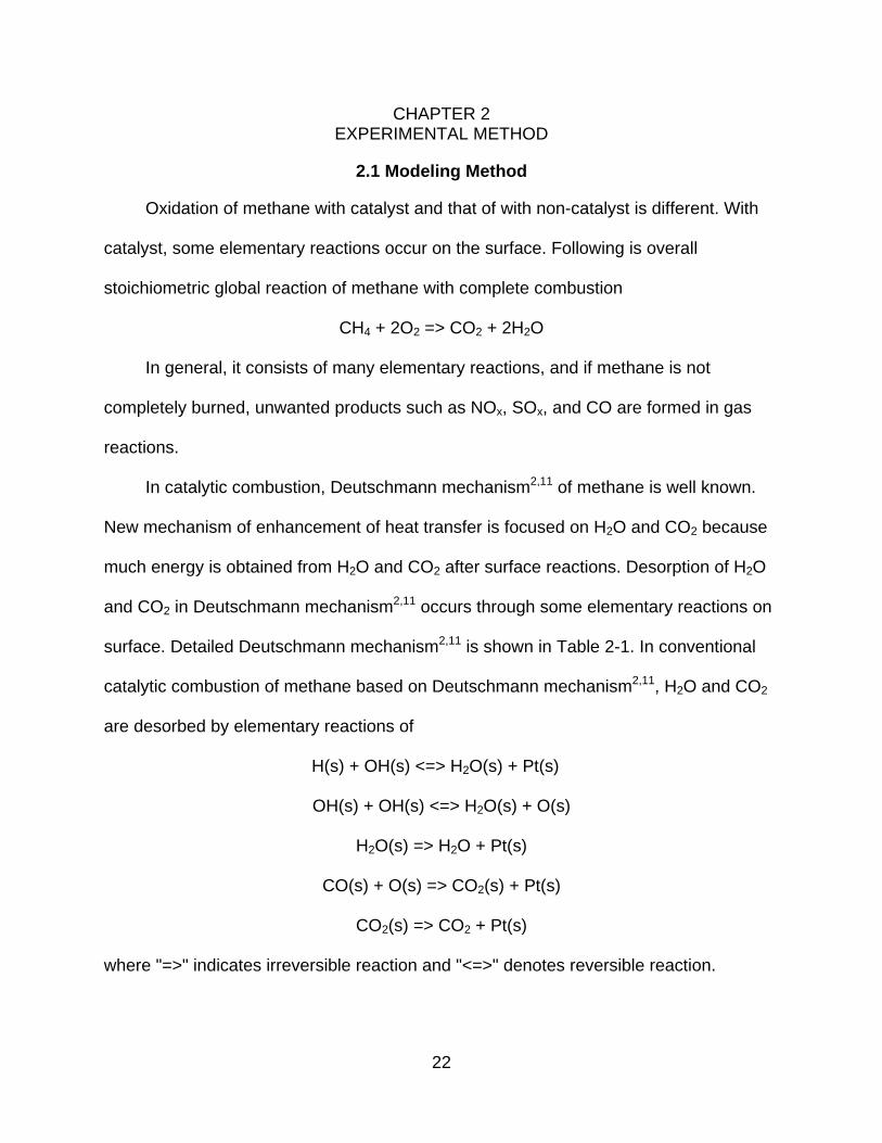
Oxidation of methane with catalyst and that of with non-catalyst is different. With
catalyst, some elementary reactions occur on the surface. Following is overall
stoichiometric global reaction of methane with complete combustion
CH4 + 2O2 => CO2 + 2H2O
In general, it consists of many elementary reactions, and if methane is not
completely burned, unwanted products such as NOx, SOx, and CO are formed in gas
reactions.
In catalytic combustion, Deutschmann mechanism2,11 of methane is well known.
New mechanism of enhancement of heat transfer is focused on H2O and CO2 because
much energy is obtained from H2O and CO2 after surface reactions. Desorption of H2O
and CO2 in Deutschmann mechanism2,11 occurs through some elementary reactions on
surface. Detailed Deutschmann mechanism2,11 is shown in Table 2-1. In conventional
catalytic combustion of methane based on Deutschmann mechanism2,11, H2O and CO2
are desorbed by elementary reactions of
H(s) + OH(s) <=> H2O(s) + Pt(s)
OH(s) + OH(s) <=> H2O(s) + O(s)
H2O(s) => H2O + Pt(s)
CO(s) + O(s) => CO2(s) + Pt(s)
CO2(s) => CO2 + Pt(s)
where "=>" indicates irreversible reaction and "<=>" denotes reversible reaction.
23
Unlike conventional catalytic combustion, mechanism of enhancement heat
transfer is started from the assumption that activated H2O and CO2 are desorbed
directly from surface without sub-reactions in Deutschmann mechanism2,11 if certain
amount of energy that exceeds activation energies of activated H2O and CO2. This
mechanism is based on GRI30 mechanism10 that is optimized mechanism and designed
to model natural gas combustion including NO formation and reburn chemistry for gas
reactions and Deutschmann mechanism2,11 for surface reactions. Therefore, some gas
reactions are added in GRI30 mechanism10 and some surface reactions are replaced
according to the assumption. To be specific, in modeling mechanism, activated H2O
whose symbol is H2O* is formed by irreversible reactions of H(S) + OH(S) and OH(S) +
OH(S) and activated H2O is dissociated into either H + OH or H2O + M. Moreover,
activated CO2 whose symbol is CO2* is formed by the reaction of irreversible CO(S) +
O(S) and it is dissociated into either CO + O or CO2 + M.
Surface reactions that forms H2O*
OH(s) + OH(s) => H2O* + O(s) + Pt(s)
H(s) + OH(s) => H2O* + 2Pt(s)
Figure 2-4 shows detailed reaction path of the reactions in modeling.
Dissociation of H2O*
H2O* => H + OH
H2O* + M => H2O + M
Here, M indicates third body reaction. Activated H2O goes to stable state by transferring
excess energy to M.
Surface reaction that forms CO2*
24
CO(s) + O(s) => CO2* + 2Pt(s)
This reaction path is shown in Figure 2-5.
Dissociation of CO2*
CO2* => CO + O
CO2* + M => CO2 + M
Activated CO2 becomes stable by giving energy to third body.
In order to attain activation energies of modeled reactions, it is assumed that the
activation energies of modeled reactions are enthalpy difference between H2O and
H2O*, and CO2 and CO2*. Moreover, two modeled reactions which are H(s) + OH(s)
<=> H2O(s) + PT(s) and CO(s) + O(s) => CO2(s) + PT(s) are considered in calculation.
Before calculating the activation energies, it is assumed that state of activated H2O and
CO2 are located at the barrier of surface reaction of H(s) + OH(s) <=> H2O(s) + PT(s)
and CO(s) + O(s) => CO2(s) + PT(s) respectively. Figure 1-5 and 1-6 shows positions of
activated H2O and CO2. Plus, it is assumed that entropy of H2O and H2O* is the same
likewise CO2 and CO2*. Enthalpy of activated H2O and CO2 are calculated by NASA
polynomials with 7 NASA coefficients. Enthalpy difference between H2O and CO2 and
H2O* and CO2* is hold constant in calculation. NASA Polynomials Equations15 are
below.
HRT
= a1 + a2T2
+ a3T2
3+ a4
T3
4+ a5
T4
5+
a6T
(2-1)
SR
= a1lnT + a2T + a3T2
2+ a4
T3
3+ a5
T4
4+ a7
(2-2)
25
CpR
= a1 + a2T + a3T2 + a4T3 + a5T4
(2-3)
where H is enthalpy that is defined as H(T) = ∆Hf(298K) + (H(T) − H(298K)) in which
∆Hf is formation of enthalpy that is the heat evolved when 1 mole of the substance is
formed from its elements in their respective standard state temperature of 298.15K, R is
universal gas constant, T(K) is temperature, S(kJ/kmol/K) is entropy, Cp(kJ/Kmol/K) is
specific heat. a1, a2, a3, a4, a5, a6 and a7 are the numerical coefficients supplied in
NASA thermodynamics files. According to the assumptions, enthalpy of H(s) and OH(s)
is calculated by NASA Polynomials of Enthalpy at 700K and by adding the activation
energy of the reaction H(s) + OH(s) <=> H2O(s) + PT(s) that is 17400 [J/mol], the state
of activated H2O is attained. As for CO2*, state of CO(s) + O(s) is calculated by NASA
Polynomials of Enthalpy at 700K, and by using the activation energy of the reaction of
CO(s) + O(s) => CO2(s) + PT(s) that is 105000 [J/mol], the enthalpy of activated CO2* is
attained. By comparing enthalpy of activation energies of H2O and CO2 with NASA
coefficient of activated H2O and CO2 which is based on H2O and CO2, NASA
coefficient of H2O* and CO2* are obtained. In order to set NASA coefficients of activated
H2O and CO2 with the same entropy, a1, a2, a3, a4,and a5 must be same as those of H2O
and CO2 respectively. Therefore a6 of activated H2O and CO2 is set to -2.909093622 x
104 and -3.213429830 x 10⁴ in low temperature range which ranges from 200K to
1000K and -2.900429710 x 10⁴ and -3.213429830 x 10⁴ in high temperature range
which ranges from 1000K to 3500K respectively based on state of H2O and CO2. Table
2-2, 2-3, 2-4, and 2-5 show NASA coefficients of H2O, H2O*, CO2, CO2*.
26
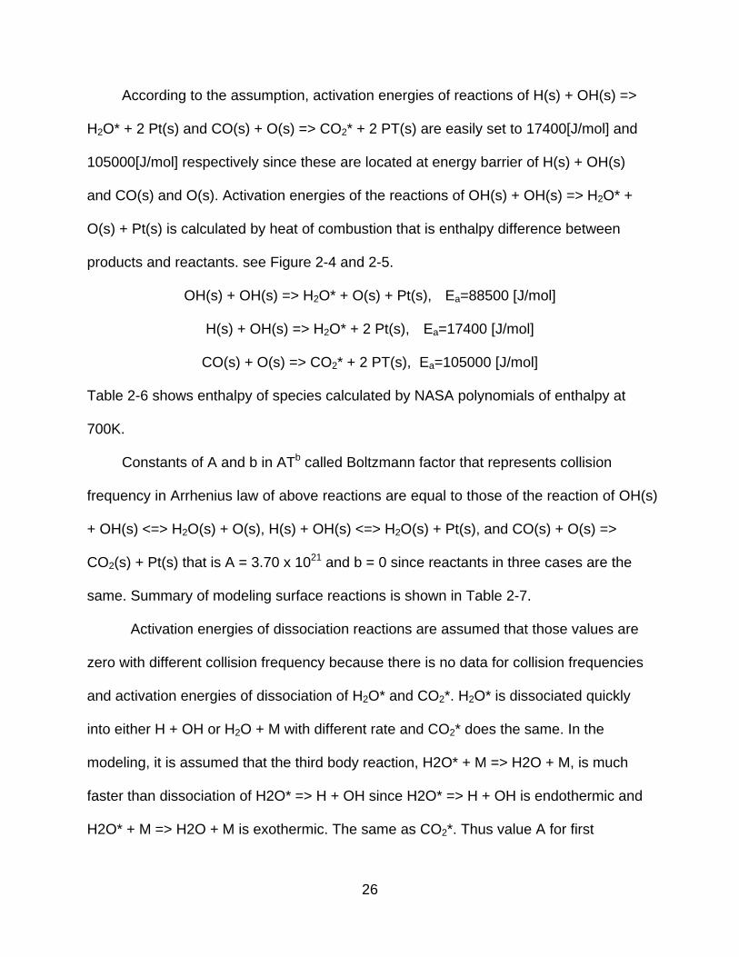
According to the assumption, activation energies of reactions of H(s) + OH(s) =>
H2O* + 2 Pt(s) and CO(s) + O(s) => CO2* + 2 PT(s) are easily set to 17400[J/mol] and
105000[J/mol] respectively since these are located at energy barrier of H(s) + OH(s)
and CO(s) and O(s). Activation energies of the reactions of OH(s) + OH(s) => H2O* +
O(s) + Pt(s) is calculated by heat of combustion that is enthalpy difference between
products and reactants. see Figure 2-4 and 2-5.
OH(s) + OH(s) => H2O* + O(s) + Pt(s), Ea=88500 [J/mol]
H(s) + OH(s) => H2O* + 2 Pt(s), Ea=17400 [J/mol]
CO(s) + O(s) => CO2* + 2 PT(s), Ea=105000 [J/mol]
Table 2-6 shows enthalpy of species calculated by NASA polynomials of enthalpy at
700K.
Constants of A and b in ATb called Boltzmann factor that represents collision
frequency in Arrhenius law of above reactions are equal to those of the reaction of OH(s)
+ OH(s) <=> H2O(s) + O(s), H(s) + OH(s) <=> H2O(s) + Pt(s), and CO(s) + O(s) =>
CO2(s) + Pt(s) that is A = 3.70 x 10²¹ and b = 0 since reactants in three cases are the
same. Summary of modeling surface reactions is shown in Table 2-7.
Activation energies of dissociation reactions are assumed that those values are
zero with different collision frequency because there is no data for collision frequencies
and activation energies of dissociation of H2O* and CO2*. H2O* is dissociated quickly
into either H + OH or H2O + M with different rate and CO2* does the same. In the
modeling, it is assumed that the third body reaction, H2O* + M => H2O + M, is much
faster than dissociation of H2O* => H + OH since H2O* => H + OH is endothermic and
H2O* + M => H2O + M is exothermic. The same as CO2*. Thus value A for first
27
dissociation reaction is set to 1.00 x 10². And value A for third body reaction is 3.00 x
108. Also, value A for CO2* => CO + O is 1.00 x 10². A for the reaction of CO2* + M =>
CO2 + M is set to 3.00 x 10⁸. Dissociation reactions are added in GRI30 mechanism10
additionally. Summary of modeled dissociation and deactivation reactions are shown in
Table 2-8.
In addition, opposite case that dissociation reaction is much faster than
deactivation reaction by the third body reaction is simulated. See Table 2-9.
In summary, three sub-reactions are replaced in Deutschmann mechanism2,11 of
surface reactions and four dissociation reactions are added in GRI30 mechanism10 for
gas reactions.
2.2 Simulation Method
Numerical simulation is conducted by Python with CANTERA17 that has been
being developed by Dr. David G. Goodwin in Division Engineering and Applied Science
in California Institution of Technology. It is being developed since 1997. It is capable of
simulating thermodynamics properties, transport properties, chemical equilibrium,
homogeneous and heterogeneous chemistry, reactor networks, one dimensional flames,
electrochemistry, and reaction path diagrams. Catalytic combustion demo that is
catcomb.py is used to simulate the modeling catalytic combustion and the conventional
catalytic combustion. It is also modified to get solution for low ignition branch. GRI30
mechanism10 is used for gas reactions and Deutschmann mechanism2,11 is used for
surface reactions. GRI30 mechanism10 consists of 325 elementary reactions and 53
species. 24 elementary surface reactions and 11 species on the surface in
Deutschmann mechanism2,11. Stagnation flow is set up in the catalytic combustion in
CANTERA17.
28
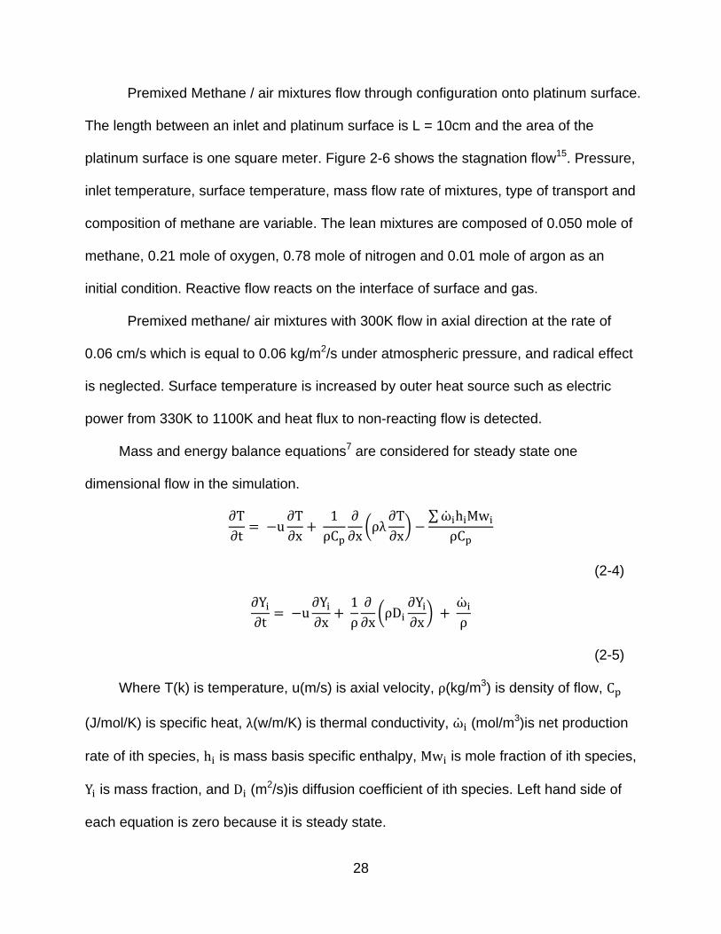
Premixed Methane / air mixtures flow through configuration onto platinum surface.
The length between an inlet and platinum surface is L = 10cm and the area of the
platinum surface is one square meter. Figure 2-6 shows the stagnation flow15. Pressure,
inlet temperature, surface temperature, mass flow rate of mixtures, type of transport and
composition of methane are variable. The lean mixtures are composed of 0.050 mole of
methane, 0.21 mole of oxygen, 0.78 mole of nitrogen and 0.01 mole of argon as an
initial condition. Reactive flow reacts on the interface of surface and gas.
Premixed methane/ air mixtures with 300K flow in axial direction at the rate of
0.06 cm/s which is equal to 0.06 kg/m2/s under atmospheric pressure, and radical effect
is neglected. Surface temperature is increased by outer heat source such as electric
power from 330K to 1100K and heat flux to non-reacting flow is detected.
Mass and energy balance equations7 are considered for steady state one
dimensional flow in the simulation.
∂T∂t
= −u∂T∂x
+ 1ρCp
∂∂x �
ρλ∂T∂x�
−∑ ωihiMwi
ρCp
(2-4)
∂Yi∂t
= −u∂Yi∂x
+ 1ρ∂∂x �
ρDi∂Yi∂x�
+ ωi
ρ
(2-5)
Where T(k) is temperature, u(m/s) is axial velocity, ρ(kg/m3) is density of flow, Cp
(J/mol/K) is specific heat, λ(w/m/K) is thermal conductivity, ωi (mol/m3)is net production
rate of ith species, hi is mass basis specific enthalpy, Mwi is mole fraction of ith species,
Yi is mass fraction, and Di (m2/s)is diffusion coefficient of ith species. Left hand side of
each equation is zero because it is steady state.
29
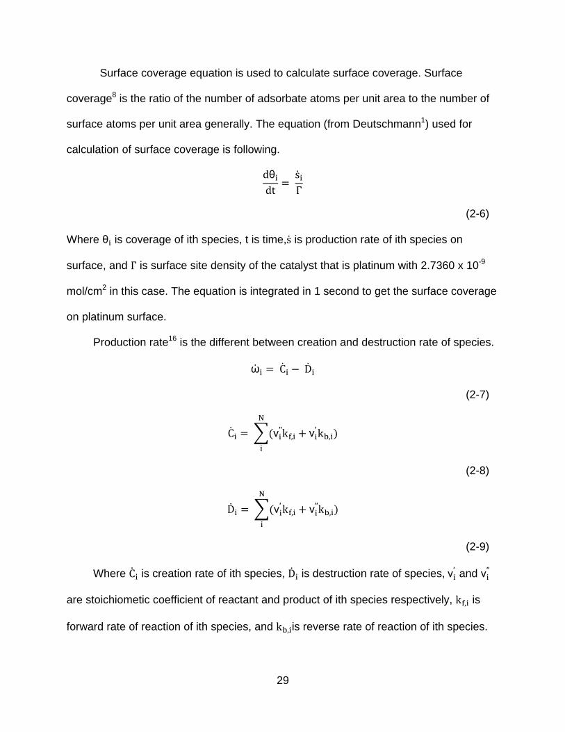
Surface coverage equation is used to calculate surface coverage. Surface
coverage8 is the ratio of the number of adsorbate atoms per unit area to the number of
surface atoms per unit area generally. The equation (from Deutschmann1) used for
calculation of surface coverage is following.
dθidt
= siГ
(2-6)
Where θi is coverage of ith species, t is time,s is production rate of ith species on
surface, and Г is surface site density of the catalyst that is platinum with 2.7360 x 10⁻⁹
mol/cm2 in this case. The equation is integrated in 1 second to get the surface coverage
on platinum surface.
Production rate16 is the different between creation and destruction rate of species.
ωi = Ci − Di
(2-7)
Ci = �(νi′′kf,i + νi′ kb,i)N
i
(2-8)
Di = �(νi′ kf,i + νi′′kb,i)N
i
(2-9)
Where Ci is creation rate of ith species, Di is destruction rate of species, νi′ and νi′′
are stoichiometic coefficient of reactant and product of ith species respectively, kf,i is
forward rate of reaction of ith species, and kb,iis reverse rate of reaction of ith species.
30
In this simulation, hydrogen/air mixtures are calculated first to use as the initial
estimate for the methane/air mixtures by using above equations. Temperature, axial
velocity, specific enthalpy, density, mole fractions of each species profiles at each grid,
and surface coverage are obtained from the simulation.
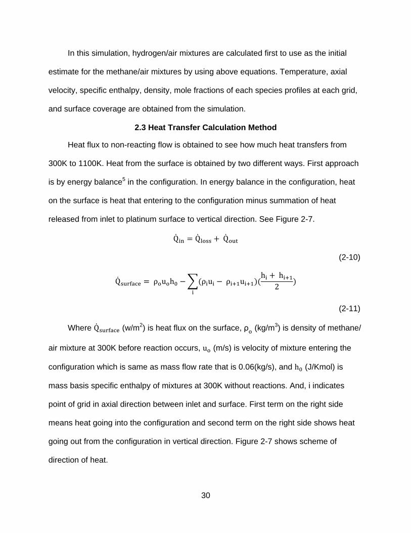
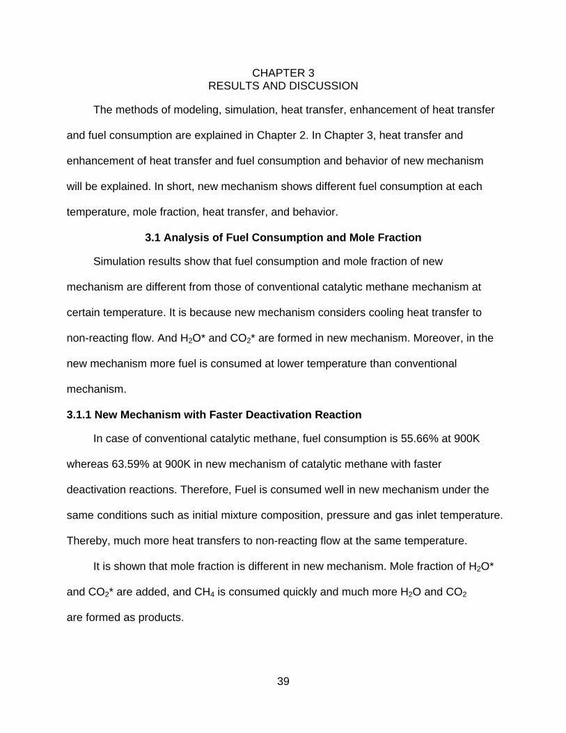
2.3 Heat Transfer Calculation Method
Heat flux to non-reacting flow is obtained to see how much heat transfers from
300K to 1100K. Heat from the surface is obtained by two different ways. First approach
is by energy balance5 in the configuration. In energy balance in the configuration, heat
on the surface is heat that entering to the configuration minus summation of heat
released from inlet to platinum surface to vertical direction. See Figure 2-7.
Qin = Qloss + Qout
(2-10)
Qsurface = ρouoh0 −�(ρiui − ρi+1ui+1)(hi + hi+1
2)
i
(2-11)
Where Qsurface (w/m2) is heat flux on the surface, ρo (kg/m3) is density of methane/
air mixture at 300K before reaction occurs, uo (m/s) is velocity of mixture entering the
configuration which is same as mass flow rate that is 0.06(kg/s), and h0 (J/Kmol) is
mass basis specific enthalpy of mixtures at 300K without reactions. And, i indicates
point of grid in axial direction between inlet and surface. First term on the right side
means heat going into the configuration and second term on the right side shows heat
going out from the configuration in vertical direction. Figure 2-7 shows scheme of
direction of heat.
31
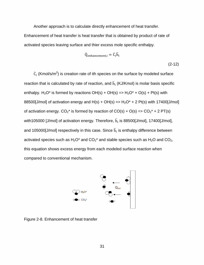
Another approach is to calculate directly enhancement of heat transfer.
Enhancement of heat transfer is heat transfer that is obtained by product of rate of
activated species leaving surface and thier excess mole specific enthalpy.
Qenhancement,i = Cih�i
(2-12)
Ci (Kmol/s/m2) is creation rate of ith species on the surface by modeled surface
reaction that is calculated by rate of reaction, and h�i (KJ/Kmol) is molar basis specific
enthalpy. H2O* is formed by reactions OH(s) + OH(s) => H2O* + O(s) + Pt(s) with
88500[J/mol] of activation energy and H(s) + OH(s) => H2O* + 2 Pt(s) with 17400[J/mol]
of activation energy. CO2* is formed by reaction of CO(s) + O(s) => CO2* + 2 PT(s)
with105000 [J/mol] of activation energy. Therefore, h�i is 88500[J/mol], 17400[J/mol],
and 105000[J/mol] respectively in this case. Since h�i is enthalpy difference between
activated species such as H2O* and CO2* and stable species such as H2O and CO2,
this equation shows excess energy from each modeled surface reaction when
compared to conventional mechanism.
Figure 2-8. Enhancement of heat transfer
32
2.4 Fuel Consumption
Fuel consumption is calculated with increasing surface temperature to see
temperature where fuel is all burnt. New mechanism shows different fuel consumption
at each temperature. Detail is explained in Chapter 3. It is calculated by product of ratio
of mass fraction of fuel at the surface to initial mass fraction of fuel at z= 0m and z=0.1m.
Equation is following.
Initial Mass Fraction of Fuel − Mass Fraction of Fuel On The SurfaceInitial Mass Fraction of Fuel
× 100
(2-13)
Briefly, modeling, simulation, heat transfer, and fuel consumption calculation
method are explained in this chapter. New mechanism is modeled with basis on
Deutschmann mechanism2,11 for surface reactions and GRI30 mechanism10 for gas
reactions with replacing and adding elementary reactions. And solution is obtained by
mass, energy balance and surface coverage equations in simulation. In addition, By
using solutions at each temperature, heat transfer on the right side of surface where
there is no reaction, enhanced heat transfer that is additional heat from surface
reactions compared to conventional catalytic combustion, and fuel consumption are
calculated to see the difference between conventional mechanism and new mechanism.
The results are explained in Chapter 3.
33
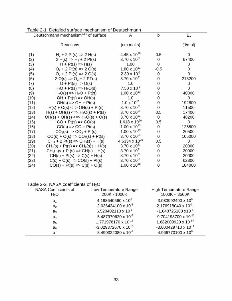
Table 2-1. Detailed surface mechanism of Deutschmann
Deutschmann mechanism2,11 of surface
Reactions
A
(cm mol s)
b Ea
(J/mol)
(1) (2) (3) (4) (5) (6) (7) (8) (9)
(10) (11) (12) (13) (14) (15) (16) (17) (18) (19) (20) (21) (22) (23) (24)
H2 + 2 Pt(s) => 2 H(s) 2 H(s) => H2 + 2 Pt(s)
H + Pt(s) => H(s) O2 + 2 Pt(s) => 2 O(s) O2 + 2 Pt(s) => 2 O(s) 2 O(s) => O2 + 2 PT(s)
O + Pt(s) => O(s) H2O + Pt(s) => H2O(s) H2O(s) => H2O + Pt(s) OH + Pt(s) => OH(s) OH(s) => OH + Pt(s)
H(s) + O(s) <=> OH(s) + Pt(s) H(s) + OH(s) <=> H2O(s) + Pt(s)
OH(s) + OH(s) <=> H2O(s) + O(s) CO + Pt(s) => CO(s) CO(s) => CO + Pt(s)
CO2(s) => CO2 + Pt(s) CO(s) + O(s) => CO2(s) + Pt(s) CH4 + 2 Pt(s) => CH3(s) + H(s)
CH3(s) + Pt(s) => CH2(s)s + H(s) CH2(s)s + Pt(s) => CH(s) + H(s)
CH(s) + Pt(s) => C(s) + H(s) C(s) + O(s) => CO(s) + Pt(s) CO(s) + Pt(s) => C(s) + O(s)
4.45 x 10¹⁰ 3.70 x 10²¹
1.00 1.80 x 10²¹ 2.30 x 10⁻² 3.70 x 10²¹
1.0 7.50 x 10⁻¹ 1.00 x 10¹³
1.0 1.0 x 10¹³
3.70 x 10²¹ 3.70 x 10²¹ 3.70 x 10²¹
1.618 x 10²⁰ 1.00 x 10¹³ 1.00 x 10¹³ 3.70 x 10²¹
4.6334 x 10²⁰ 3.70 x 10²¹ 3.70 x 10²¹ 3.70 x 10²¹ 3.70 x 10²¹ 1.00 x 10¹⁸
0.5 0 0
-0.5 0 0 0 0 0 0 0 0
0.5 0
0.5 0 0 0
0.5 0 0 0 0 0
0 67400
0 0 0
213200 0 0
40300 0
192800 11500 17400 48200
0 125500 20500
105000 0
20000 20000 20000 62800
184000
Table 2-2. NASA coefficients of H2O
NASA Coefficients of H2O
Low Temperature Range 200K - 1000K
High Temperature Range 1000K – 3500K
a1 4.198640560 x 100 3.033992490 x 100 a2 -2.036434100 x 10⁻³ 2.176918040 x 10⁻³, a3 6.520402110 x 10⁻⁶ -1.640725180 x10⁻⁷ a4 -5.487970620 x 10⁻⁹ -9.704198700 x 10⁻¹¹ a5 1.771978170 x 10⁻¹² 1.682009920 x 10⁻¹⁴ a6 -3.029372670 x 10+4 -3.000429710 x 10+4 a7 -8.490322080 x 10⁻¹ 4.966770100 x 100
34
Table 2-3. NASA coefficients of H2O* NASA Coefficients of
H2O* Low Temperature Range
200K - 1000K High Temperature Range
1000K – 3500K a1 4.198640560 x 100 3.033992490 x 100 a2 -2.036434100 x 10⁻³ 2.176918040 x 10⁻³, a3 6.520402110 x 10⁻⁶ -1.640725180 x10⁻⁷ a4 -5.487970620 x 10⁻⁹ -9.704198700 x 10⁻¹¹ a5 1.771978170 x 10⁻¹² 1.682009920 x 10⁻¹⁴ a6 -2.909093622 x 10+4 -2.900429710 x 10+4 a7 -8.490322080 x 10⁻¹ 4.966770100 x 100
Table 2-4. NASA coefficients of CO2 NASA Coefficients of
CO2 Low Temperature Range
200K - 1000K High Temperature Range
1000K – 3500K a1 2.356773520 x 100 3.857460290 x 100 a2 8.984596770 x 10⁻³ 4.414370260 x 10⁻³ a3 -7.123562690 x 10⁻⁶ -2.214814040 x 10⁻⁶ a4 2.459190220 x 10⁻⁹ 5.234901880 x 10⁻¹⁰ a5 -1.436995480 x 10⁻¹³ -4.720841640 x 10⁻¹⁴ a6 -4.837196970x 10+4 -4.875916600 x 10⁻¹⁴ a7 9.901052220 x 100 2.271638060 x 100
Table 2-5. NASA coefficients of CO2*
NASA Coefficients of CO2*
Low Temperature Range 200K - 1000K
High Temperature Range 1000K – 3500K
a1 2.356773520 x 100 3.857460290 x 100 a2 8.984596770 x 10⁻³ 4.414370260 x 10⁻³ a3 -7.123562690 x 10⁻⁶ -2.214814040 x 10⁻⁶ a4 2.459190220 x 10⁻⁹ 5.234901880 x 10⁻¹⁰ a5 -1.436995480 x 10⁻¹³ -4.720841640 x 10⁻¹⁴ a6 -3.213429830 x 10+4 -3.213429830 x 10⁻¹⁴ a7 9.901052220 x 100 2.271638060 x 100
Table 2-6. Enthalpy of species at 700K. H is calculated by (H/RT)*RT where R is gas constant that is 8.314[J/mol/K] and T is temperature. Species H/RT H [J/mol]
H(s) -5.61807343242547 -32696.0638 OH(s) -35.1834824436407 -204760.8311 CO(s) -41.1300311398638 -239368.5552 O(s) -41.1300311398638 -103372.7744 Pt(s) 0 0 H2O* -37.3930957669273 -217620.3387 H2O -39.111367881213 -227620.3388 CO2* -41.364298169368 -240731.9425 CO2 -64.5609715979394 -375731.9425
35
Table 2-7. Surface reactions in new mechanism Surface Reaction Mechanism
Of Modeling A
(cm mol s) b Ea
(J/mol) (1) (2) (3) (4) (5) (6) (7) (8) (9)
(10) (11) (12) (13) (14) (15) (16) (17) (18) (19) (20) (21) (22) (23) (24)
H2 + 2 Pt(s) => 2 H(s) 2 H(s) => H2 + 2 Pt(s)
H + Pt(s) => H(s) O2 + 2 Pt(s) => 2 O(s) O2 + 2 Pt(s) => 2 O(s) 2 O(s) => O2 + 2 PT(s)
O + Pt(s) => O(s) H2O + Pt(s) => H2O(s) H2O(s) => H2O + Pt(s) OH + Pt(s) => OH(s) OH(s) => OH + Pt(s)
H(s) + O(s) <=> OH(s) + Pt(s) CO + Pt(s) => CO(s) CO(s) => CO + Pt(s)
CO2(s) => CO2 + Pt(s) CH4 + 2 Pt(s) => CH3(s) + H(s)
CH3(s) + Pt(s) => CH2(s)s + H(s) CH2(s)s + Pt(s) => CH(s) + H(s)
CH(s) + Pt(s) => C(s) + H(s) C(s) + O(s) => CO(s) + Pt(s) CO(s) + Pt(s) => C(s) + O(s)
OH(s) + OH(s) => H2O* + O(s) +Pt(s) H(s) + OH(s) => H2O* + 2 PT(s) CO(s) + O(s) => CO2* + 2 PT(s)
4.45 x 10¹⁰ 3.70 x 10²¹
1.00 1.80 x 10²¹ 2.30 x 10⁻² 3.70 x 10²¹
1.0 7.50 x 10⁻¹ 1.00 x 10¹³
1.0 1.0 x 10¹³
3.70 x 10²¹
1.618 x 10²⁰ 1.00 x 10¹³ 1.00 x 10¹³
4.6334 x 10²⁰ 3.70 x 10²¹ 3.70 x 10²¹ 3.70 x 10²¹ 3.70 x 10²¹ 1.00 x 10¹⁸ 3.70 x 10²¹ 3.70 x 10²¹ 3.70 x 10²¹
0.5 0 0
-0.5 0 0 0 0 0 0 0 0
0.5 0 0
0.5 0 0 0 0 0 0 0 0
0 67400
0 0 0
213200 0 0
40300 0
192800 11500
0 125500 20500
0 20000 20000 20000 62800
184000 88500 17400
105000
Table 2-8. Gas reactions in new mechanism with faster deactivation reaction Dissociation Reactions in Modeling A
(cm mol s) b Ea
(J/mol) (1) (2) (3) (4)
H2O* => H + OH H2O* + M => H2O + M
CO2* => CO + O CO2* + M => CO2 + M
1.00 x 10² 3.00 x 10⁸ 1.00 x 10² 3.00 x 10⁸
0 0 0 0
0 0 0 0
36
Table 2-9. Gas reactions in new mechanism with the faster dissociation reaction Dissociation Reactions in Modeling A
(cm mol s) b Ea
(J/mol) (1) (2) (3) (4)
H2O* => H + OH H2O* + M => H2O + M
CO2* => CO + O CO2* + M => CO2 + M
3.00 x 10³ 0.10 x 101 3.00 x 10³ 0.10 x 101
0 0 0 0
0 0 0 0
Figure 2-1. Reaction path of H(s) + OH(s) in Deutschmann mechanism. Ea1 indicates
activation energy of reaction of H(s) + OH(s) and Ea2 indicates activation energy of desorption of reaction of H2O(s).(Ea1=17400J/mol, and Ea2=40300J/mol)
Figure 2-2. Reaction path of OH(s) + OH(s) and H2O(s) in Deutschmann mechanism.
Ea1 is 48200J/mol and Ea2 is 40300J/mol.
37
Figure 2-3. Reaction path of CO(s) + O(s) and CO2(s) in Deutschmann mechanism. Ea1 is 105000J/mol and Ea2 is 20500J/mol.
Figure 2-4. Left picture shows reaction path of reaction of H(s) + O(s) in modeling. Ea1 indicates activation energy of reaction H(s) + OH(s) => H2O. Dashed line show reaction path of modeling. Line is conventional reaction path. Right figure shows reaction path of reaction of H(s) + OH(s) => H2O* + 2pt(s). Ea1 indicates activation energy of above reaction.
Figure 2-5. Reaction path of CO(s) + O(s) in modeling. Dashed line shows reaction path of modeling. Ea1 is activation energy of reaction of CO(s) + O(s) => CO2* + 2Pt(s), and the line shows conventional reaction path.
38
Figure 2-6. Stagnation flow
Figure 2-7. Energy balance
39
CHAPTER 3 RESULTS AND DISCUSSION
The methods of modeling, simulation, heat transfer, enhancement of heat transfer
and fuel consumption are explained in Chapter 2. In Chapter 3, heat transfer and
enhancement of heat transfer and fuel consumption and behavior of new mechanism
will be explained. In short, new mechanism shows different fuel consumption at each
temperature, mole fraction, heat transfer, and behavior.
3.1 Analysis of Fuel Consumption and Mole Fraction
Simulation results show that fuel consumption and mole fraction of new
mechanism are different from those of conventional catalytic methane mechanism at
certain temperature. It is because new mechanism considers cooling heat transfer to
non-reacting flow. And H2O* and CO2* are formed in new mechanism. Moreover, in the
new mechanism more fuel is consumed at lower temperature than conventional
mechanism.
3.1.1 New Mechanism with Faster Deactivation Reaction
In case of conventional catalytic methane, fuel consumption is 55.66% at 900K
whereas 63.59% at 900K in new mechanism of catalytic methane with faster
deactivation reactions. Therefore, Fuel is consumed well in new mechanism under the
same conditions such as initial mixture composition, pressure and gas inlet temperature.
Thereby, much more heat transfers to non-reacting flow at the same temperature.
It is shown that mole fraction is different in new mechanism. Mole fraction of H2O*
and CO2* are added, and CH4 is consumed quickly and much more H2O and CO2
are formed as products.
40
3.1.2 New Mechanism with Faster Dissociation Reaction
In case of new mechanism with faster dissociation reaction, fuel consumption is
99.35% at 900K whereas all of methane consumed around 1100K in conventional case.
This case shows the most fuel consumption amoung the mechanisms. Therefore,the
most fuel is consumed in new mechanism with faster dissociation reactions under the
same conditions such as initial mixture composition, pressure and gas inlet temperature.
Thereby, the most heat transfers to non-reacting flow at the same temperature.
Compared to those two mechanism, CH4 is consumed more quickly and the most
H2O and CO2 are formed as products at the same temperature.
3.2 Analysis of Heat Transfer
Heat flux to non-reacting flow is calculated by global energy balance equation5 by
increasing surface temperature from 300K to 1100K.
3.2.1 New Mechanism with Faster Deactication Reaction
In conventional catalytic methane, it shows that surface reactions start to occur at
760K since heat transfer to non-reacting flow starts to increase with increasing surface
temperature while some surface reactions start at 750K in new mechanism.
Conventional catalytic methane shows that ignition occurs around 930K because since
930K heat is released from reactions whereas new mechanism of catalytic methane
shows that ignition occurs around 913K. Result of heat transfer to non-reacting flow
shows that in conventional catalytic methane with respect to heat transfer, heat should
be added by about 930K to make ignition occur, when surface temperature is over 930K,
heat is started to released to non-reacting flow. The Figure 3-16 shows heat flux to the
non-reacting flow.
41
In new mechanism, the shape of graph is similar to that in conventional catalytic
methane. Detailed heat flux is shown in Figure 3-17. However, heat transfer to non-
reacting flow is slightly larger than that in conventional catalytic mechanism. It is
because there is excess heat transfer from adsorption and desorption of species such
as H2O* and CO2*. When compared to conventional catalytic mechanism, it shows that
heat transfer to non-reacting flow is similar to that of conventional catalytic mechanism
by 730K. This means that surface reactions that form H2O* and CO2* are inactive.
However, slight difference of heat transfer to non-reacting flow starts to show since
730K and it is larger as surface temperature is increased since surface reactions of
OH(s) + OH(s) => H2O* + O(s) + Pt(s), H(s) + OH(s) => H2O* + 2 Pt(s), and CO(s) +
O(s) => CO2* + 2 PT(s) start to occurs around 730K. After 1070K, heat transfer to non-
reacting flow is suddenly increased as surface temperature is increased since at high
temperature, gas reactions are dominant. See Figure 3-17 and Figure 3-18.
Excess heat from the surface reaction that forms H2O* and CO2* is almost zero by
700K. After 700K excess heat from surface reactions starts to generate. Then, excess
heat is suddenly increases as surface temperature is increased. Therefore,
enhancement of heat transfer due to surface reactions results in slight difference of heat
transfer to non-reacting flow between new mechanism and conventional catalytic
mechanism. This means that much heat can be obtained from the reactions of OH(s) +
OH(s) => H2O* + O(s) + Pt(s), H(s) + OH(s) => H2O* + 2 Pt(s), and CO(s) + O(s) =>
CO2* + 2 PT(s). At 990K enhancement of heat transfer to non-reacting flow starts to
decrease and after 1070K it is suddenly drop with increasing surface temperature since
at high temperature gas reactions are dominant. See Figure 3-19.
42
3.2.2 New Mechanism with Faster Dissociation Reaction
Unlike heat transfer of conventional catalytic methane, new mechanism with faster
dissociation reaction consists of high and low ignition branch. Detailed heat flux is
shown in Figure 3-20. Heat transfer to non-reacting flow is calculated by increasing
surface temperature from 300K to 1100K.
In the low ignition branch, surface reaction is dominant but weak. Therefore, radicals
such as H, O, OH, H2O, CO2 come off from the surface. As surface temperature
increases from 300K, more heat is needed to light off in low ignition branch. Heat
transfer between 918K and 936K shows unusual phenomenon. Much more heat is
needed to maintain surface temperature. This has not been discovered in this study.
More experimental reserach is needed to find the reason. At 1015.2K, small amount of
heat is needed. This means that ignition occurs at this temperature, and reactions
suddenly jump to the high ignition branch. In high branch, surface temperature should
be cooled down to maintain combustion. More decreasing surface temperature leads to
extinguishing flame at 616.5K with jumping to low branch. The reason why the amount
of heat released from surface is suddenly increased from 1075K to 1080K is that even
though gas reaction is dominant at this temperature, there is some of surface reaction,
but at 1080K, there is no surface reaction at all. By repeating increasing and decreasing
surface temperature, it shows auto-thermal phenomenon. Combustion circulates from
1015.2K to 616.2K in the high branch and from 616.2K to 1015.2K in the low branch.
When compared to heat transfer of conventional catalytic methane, it shows that much
more complete combustion from 616.6K to 1015.2K after ignition occurs.
Excess heat from the surface reaction that forms H2O* and CO2* is almost zero in
low branch whereas in high branch much heat is released from the surface. This means
43
that much heat can be obtained from the reactions of OH(s) + OH(s) => H2O* + O(s) +
Pt(s), H(s) + OH(s) => H2O* + 2 Pt(s), and CO(s) + O(s) => CO2* + 2 PT(s). Figure 3-21
shows enhancement of heat transfer.
Heat flux to non-reacting flow by global energy balance is different from that by
enhancement of heat transfer. It shows that enhancement of heat flux is three times
larger than heat transfer by global energy balance. Thus, according to this mechanism,
more heat is obtained from surface reactions compared to conventional mechanism.
Finally, more experimental works are required to get collision frequency and activation
energy of modeled dissociation reactions and to correct new mechanism.
44
Figure 3-1. Mole fraction of species in Deutschmann at 900K
Figure 3-2. Axial velocity profile in Deutschmann at 900K
Figure 3-3. Temperature profile in Deutschmann at 900K
45
Figure 3-4. Density profile in Deutschmann at 900K
Figure 3-5. Specific enthalpy in Deutschmann at 900K
46
Figure 3-6. Mole fraction of species in new mechanism with faster deactivation at 900K
Figure 3-7. Axial velocity profile in new mechanism with faster deactivation at 900K
Figure 3-8. Temperature profile in new mechanism with faster deactivation at 900K
47
Figure 3-9. Density profile in new mechanism with faster deactivation at 900K
Figure 3-10. Specific enthalpy in new mechanism with faster deactivation at 900K
48
Figure 3-11. Mole fraction of species in new mechanism with faster dissociation at 900K
Figure 3-12. Axial velocity profile in new mechanism with faster dissociation at 900K
Figure 3-13. Temperature profile in new mechanism with faster dissociation at 900K
49
Figure 3-14. Density profile in new mechanism with faster dissociation at 900K
Figure 3-15. Specific enthalpy in new mechanism with faster dissociation at 900K
50
Figure 3-16. Heat transfer to non-reacting flow in Deutschmann
Figure 3-17. Heat transfer to non-reacting flow in new mechanism with faster deactivation
51
Figure 3-18. Heat transfer to non-reacting flow in conventional and new mechanism
Figure 3-19. Enhancement of heat transfer in new mechanism with faster deactivation
52
Figure 3-20. Heat transfer to non-reacting flow in new mechanism with faster dissociation
Figure 3-21. Enhancement of heat transfer in new mechanism with faster dissociation
53
CHAPTER 4 SUMMARY
This mechanism of catalytic methane is postulated mechanism. New mechanism of
catalytic methane under enhancement heat transfer is based on GRI30 mechanism10 for
gas reactions and Deutschmann mechanism2,11 for surface reaction. This mechanism
much more focuses on enhancement of heat transfer than combustion of reacting flow.
Activated H2O and CO2 are desorbed directly from surface reactions and dissociated or
deactivated into either H2O or H + OH, and either CO2 or CO + O with different collision
frequency but zero activation energy. More experimental work is needed to measure
activation energies and collision frequency of dissociation reactions of activated H2O
and CO2 to correct this mechanism. Main features of new mechanism are following.
OH(s) + OH(s) => H2O* + O(s) +Pt(s)
H(s) + OH(s) => H2O* + 2 PT(s)
CO(s) + O(s) => CO2* + 2 PT(s)
Those surface reactions represent that activated H2O and CO2 are desorbed directly
from surface.
H2O* => H + OH
H2O* + M => H2O + M
CO2* => CO + O
CO2* + M => CO2 + M
Those gas reactions represents dissociation of activated H2O and CO2 with different
rate of reaction and zero activation energy in which dissociation reaction occurs
automatically without putting energy.
54
From the simulation, new mechanism shows different path. In New mechanism
with faster deactivation, heat flux to non-reacting flow shows similar to conventional
catalytic methane mechanism, but slightly more heat transfers to non-reacting flow due
to enhancement of heat transfer. Moreover, enhancement of heat transfer starts around
730K and increases with increasing surface temperature by 1000K and then starts to
decrease and is suddenly decrease to zero at 1100K since gas reactions are dominant
at high temperature. In New Mechanism with faster dissociation, it consists of two
different branches that is high and low ignition branch. Heat is put into surface by
1015.2K to ignite, and then reactions suddenly occur with jumping to high branch. After
ignition occurs, surface should be cooled down by 616.5K and then jump to the low
branch. In order to make automatically circulate combustion process in this region,
heating process and cooling process are needed at low branch and high branch
respectively.
Amount of heat transfer to non-reacting flow in new mechanism is higher than
that in conventional catalytic methane mechanism due to enhancement of heat transfer.
And enhancement of heat transfer where excess heat is released from modeled
surface reactions is significantly different from heat flux that is calculated by global
energy balance equation. This means that classic conventional heat transfer is needed
to be corrected under surface reactions. Moreover, heat transfer to non-reacting flow is
different in new mechanism according to rate of reactions of dissociation and
deactivation. Finally, much more research is required to improve this new mechanism.
55
APPENDIX A ORIGINAL CATCOMB CODE
# CATCOMB -- Catalytic combustion of methane on platinum. # # This script solves a catalytic combustion problem. A stagnation flow # is set up, with a gas inlet 10 cm from a platinum surface at 900 # K. The lean, premixed methane/air mixture enters at ~ 6 cm/s (0.06 # kg/m2/s), and burns catalytically on the platinum surface. Gas-phase # chemistry is included too, and has some effect very near the # surface. # # The catalytic combustion mechanism is from Deutschman et al., 26th # Symp. (Intl.) on Combustion,1996 pp. 1747-1754 # # from Cantera import * from Cantera.OneD import * #from Cantera.OneD.StagnationFlow import StagnationFlow import math ############################################################### # # Parameter values are collected here to make it easier to modify # them p = OneAtm # pressure tinlet = 300.0 # Inlet temperature tsurf = 900.0 # surface temperature mdot = 0.06 # kg/m^2/s transport = 'Mix' # transport model # We will solve first for a hydrogen/air case to # use as the initial estimate for the methane/air case # composition of the inlet premixed gas for the hydrogen/air case comp1 = 'H2:0.05, O2:0.21, N2:0.78, AR:0.01' # composition of the inlet premixed gas for the methane/air case comp2 = 'CH4:0.050, O2:0.21, N2:0.78, AR:0.01' # the initial grid, in meters. The inlet/surface separation is 10 cm. initial_grid = [0.0, 0.02, 0.04, 0.06, 0.08, 0.1] # m
56
# numerical parameters tol_ss = [1.0e-5, 1.0e-9] # [rtol, atol] for steady-state problem tol_ts = [1.0e-4, 1.0e-9] # [rtol, atol] for time stepping loglevel = 5 # amount of diagnostic output # (0 to 5) refine_grid = 1 # 1 to enable refinement, 0 to # disable ################ create the gas object ######################## # # This object will be used to evaluate all thermodynamic, kinetic, # and transport properties # # The gas phase will be taken from the definition of phase 'gas' in # input file 'ptcombust.cti,' which is a stripped-down version of # GRI-Mech 3.0. gas = importPhase('ptcombust.cti','gas') gas.set(T = tinlet, P = p, X = comp1) ################ create the interface object ################## # # This object will be used to evaluate all surface chemical production # rates. It will be created from the interface definition 'Pt_surf' # in input file 'ptcombust.cti,' which implements the reaction # mechanism of Deutschmann et al., 1995 for catalytic combustion on # platinum. # surf_phase = importInterface('ptcombust.cti','Pt_surf', [gas]) surf_phase.setTemperature(tsurf) # integrate the coverage equations in time for 1 s, holding the gas # composition fixed to generate a good starting estimate for the # coverages. surf_phase.advanceCoverages(1.0) # create the object that simulates the stagnation flow, and specify an # initial grid sim = StagnationFlow(gas = gas, surfchem = surf_phase, grid = initial_grid) # Objects of class StagnationFlow have members that represent the gas inlet ('inlet') and the surface ('surface'). Set some parameters of these objects.
57
sim.inlet.set(mdot = mdot, T = tinlet, X = comp1) sim.surface.set(T = tsurf) # Set error tolerances sim.set(tol = tol_ss, tol_time = tol_ts) # Method 'init' must be called before beginning a simulation sim.init() # Show the initial solution estimate sim.showSolution() # Solving problems with stiff chemistry coulpled to flow can require # a sequential approach where solutions are first obtained for # simpler problems and used as the initial guess for more difficult # problems. # start with the energy equation on (default is 'off') sim.set(energy = 'on') # disable the surface coverage equations, and turn off all gas and # surface chemistry. sim.surface.setCoverageEqs('off') surf_phase.setMultiplier(0.0); gas.setMultiplier(0.0); # solve the problem, refining the grid if needed, to determine the # non-reacting velocity and temperature distributions sim.solve(loglevel, refine_grid) # now turn on the surface coverage equations, and turn the # chemistry on slowly sim.surface.setCoverageEqs('on') for iter in range(6): mult = math.pow(10.0,(iter - 5)); surf_phase.setMultiplier(mult); gas.setMultiplier(mult); print 'Multiplier = ',mult sim.solve(loglevel, refine_grid); # At this point, we should have the solution for the hydrogen/air # problem. sim.showSolution()
58
# Now switch the inlet to the methane/air composition. sim.inlet.set(X = comp2) # set more stringent grid refinement criteria sim.setRefineCriteria(100.0, 0.15, 0.2, 0.0) # solve the problem for the final time sim.solve(loglevel, refine_grid) # show the solution sim.showSolution() # save the solution in XML format. The 'restore' method can be used to restart # a simulation from a solution stored in this form. sim.save("catcomb.xml","sol") # save selected solution components in a CSV file for plotting in # Excel or MATLAB. # These methods return arrays containing the values at all grid points z = sim.flow.grid() T = sim.T() u = sim.u() V = sim.V() f = open('catcomb.csv','w') writeCSV(f, ['z (m)', 'u (m/s)', 'V (1/s)', 'T (K)','Tc(K)', 'rho (kg/m3)', 'specific enthalpy (J/kg)','thermal conducticity (w/m2 k)'] + list(gas.speciesNames())+ list(gas.speciesNames())) for n in range(sim.flow.nPoints()): Tc=((T[n]-300)*tsurf)/(tsurf-tinlet) + 300 sim.setGasState(n) writeCSV(f, [z[n], u[n], V[n], T[n], Tc, gas.density(), gas.enthalpy_mass(), gas.thermalConductivity()] +list(gas.moleFractions()) +list(gas.creationRates())) # write the surface coverages to the CSV file writeCSV(f, ['species on the surface','converages','concentrations']) cov = sim.coverages() con = surf_phase.concentrations()
59
names = surf_phase.speciesNames() for n in range(len(names)): writeCSV(f, [names[n], cov[n],con[n]]) for n in range(24): rxn=surf_phase.reactionEqn(n) writeCSV(f, list([rxn])) writeCSV(f,['fwdrateconst'] +list(surf_phase.fwdRateConstants())) writeCSV(f,['fwdrateprogress'] +list(surf_phase.fwdRatesOfProgress())) writeCSV(f,['species on the surface'] +list(gas.speciesNames()) +list(surf_phase.speciesNames())) writeCSV(f,['nasa enthalpies'] +list(gas.enthalpies_RT()) +list(surf_phase.enthalpies_RT())) writeCSV(f,['creationRate on the surface'] +list(surf_phase.creationRates())) writeCSV(f,['destructionRate on the surface'] +list(surf_phase.destructionRates())) writeCSV(f,['netproductionRate on the surface'] +list(surf_phase.netProductionRates())) f.close() print 'solution saved to catcomb.csv' # show some statistics sim.showStats()
60
APPENDIX B MODIFIED CATCOMB CODE FOR LOW IGNITION BRANCH
# CATCOMB -- Catalytic combustion of methane on platinum. # # This script solves a catalytic combustion problem. A stagnation flow # is set up, with a gas inlet 10 cm from a platinum surface at 900 # K. The lean, premixed methane/air mixture enters at ~ 6 cm/s (0.06 # kg/m2/s), and burns catalytically on the platinum surface. Gas-phase # chemistry is included too, and has some effect very near the # surface. # # The catalytic combustion mechanism is from Deutschman et al., 26th # Symp. (Intl.) on Combustion,1996 pp. 1747-1754 # # from Cantera import * from Cantera.OneD import * #from Cantera.OneD.StagnationFlow import StagnationFlow import math ############################################################### # # Parameter values are collected here to make it easier to modify # them p = OneAtm # pressure tinlet = 300.0 # Inlet temperature tstart = 700.0 # starting temperature tsurf = 1016.0 # surface temperature mdot = 0.06 # kg/m^2/s i = 1.0 # Increment of Surface Temperature transport = 'Mix' # transport model # We will solve first for a hydrogen/air case to # use as the initial estimate for the methane/air case # composition of the inlet premixed gas for the hydrogen/air case comp1 = 'H2:0.05, O2:0.21, N2:0.78, AR:0.01' # composition of the inlet premixed gas for the methane/air case comp2 = 'CH4:0.050, O2:0.21, N2:0.78, AR:0.01' # the initial grid, in meters. The inlet/surface separation is 10 cm.
61
initial_grid = [0.0, 0.02, 0.04, 0.06, 0.08, 0.1] # m # numerical parameters tol_ss = [1.0e-10, 1.0e-10] # [rtol, atol] for steady-state problem tol_ts = [1.0e-4, 1.0e-9] # [rtol, atol] for time stepping loglevel = 2 # amount of diagnostic output # (0 to 5) refine_grid = 1 # 1 to enable refinement, 0 to # disable ################ create the gas object ######################## # # This object will be used to evaluate all thermodynamic, kinetic, # and transport properties # # The gas phase will be taken from the definition of phase 'gas' in # input file 'ptcombust.cti,' which is a stripped-down version of # GRI-Mech 3.0. gas = importPhase('ptcombust.cti','gas') gas.set(T = tinlet, P = p, X = comp1) ################ create the interface object ################## # # This object will be used to evaluate all surface chemical production # rates. It will be created from the interface definition 'Pt_surf' # in input file 'ptcombust.cti,' which implements the reaction # mechanism of Deutschmann et al., 1995 for catalytic combustion on # platinum. # surf_phase = importInterface('ptcombust.cti','Pt_surf', [gas]) surf_phase.setTemperature(481) surf_phase.advanceCoverages(1.0) sim = StagnationFlow(gas = gas, surfchem = surf_phase, grid = initial_grid) sim.inlet.set(mdot = mdot, T = tinlet, X = comp1) sim.surface.set(T = 481) sim.set(tol = tol_ss, tol_time = tol_ts) sim.init() sim.showSolution() sim.set(energy = 'on') sim.surface.setCoverageEqs('off')
62
surf_phase.setMultiplier(0.0); gas.setMultiplier(0.0); sim.solve(loglevel, refine_grid) sim.surface.setCoverageEqs('on') for iter in range(6): mult = math.pow(10.0,(iter - 5)); surf_phase.setMultiplier(mult); gas.setMultiplier(mult); print 'Multiplier = ',mult sim.solve(loglevel, refine_grid); sim.showSolution() sim.inlet.set(X = comp2) sim.setRefineCriteria(100.0, 0.15, 0.2, 0.0) sim.solve(loglevel, refine_grid) sim.showSolution() surf_phase.setTemperature(500) surf_phase.advanceCoverages(1.0) sim = StagnationFlow(gas = gas, surfchem = surf_phase, grid = initial_grid) sim.inlet.set(mdot = mdot, T = tinlet, X = comp1) sim.surface.set(T = 500) sim.set(tol = tol_ss, tol_time = tol_ts) sim.init() sim.showSolution() sim.set(energy = 'on') sim.surface.setCoverageEqs('off') surf_phase.setMultiplier(0.0); gas.setMultiplier(0.0); sim.solve(loglevel, refine_grid) sim.surface.setCoverageEqs('on') for iter in range(6): mult = math.pow(10.0,(iter - 5)); surf_phase.setMultiplier(mult); gas.setMultiplier(mult); print 'Multiplier = ',mult sim.solve(loglevel, refine_grid); sim.showSolution() sim.inlet.set(X = comp2) sim.setRefineCriteria(100.0, 0.15, 0.2, 0.0) sim.solve(loglevel, refine_grid) sim.showSolution() surf_phase.setTemperature(600) surf_phase.advanceCoverages(1.0) sim = StagnationFlow(gas = gas, surfchem = surf_phase,
63
grid = initial_grid) sim.inlet.set(mdot = mdot, T = tinlet, X = comp1) sim.surface.set(T = 600) sim.set(tol = tol_ss, tol_time = tol_ts) sim.init() sim.showSolution() sim.set(energy = 'on') sim.surface.setCoverageEqs('off') surf_phase.setMultiplier(0.0); gas.setMultiplier(0.0); sim.solve(loglevel, refine_grid) sim.surface.setCoverageEqs('on') for iter in range(6): mult = math.pow(10.0,(iter - 5)); surf_phase.setMultiplier(mult); gas.setMultiplier(mult); print 'Multiplier = ',mult sim.solve(loglevel, refine_grid); sim.showSolution() sim.inlet.set(X = comp2) sim.setRefineCriteria(100.0, 0.15, 0.2, 0.0) sim.solve(loglevel, refine_grid) sim.showSolution() while tstart < tsurf: tstart=tstart+ i surf_phase.setTemperature(tstart) surf_phase.advanceCoverages(1.0) sim = StagnationFlow(gas = gas, surfchem = surf_phase, grid = initial_grid) sim.inlet.set(mdot = mdot, T = tinlet, X = comp1) sim.surface.set(T = tstart) sim.set(tol = tol_ss, tol_time = tol_ts) sim.init() sim.showSolution() sim.set(energy = 'on') sim.surface.setCoverageEqs('off') surf_phase.setMultiplier(0.0); gas.setMultiplier(0.0); sim.solve(loglevel, refine_grid) sim.surface.setCoverageEqs('on') for iter in range(6): mult = math.pow(10.0,(iter - 5)); surf_phase.setMultiplier(mult); gas.setMultiplier(mult); print 'Multiplier = ',mult sim.solve(loglevel, refine_grid);
64
sim.showSolution() sim.inlet.set(X = comp2) sim.setRefineCriteria(100.0, 0.15, 0.2, 0.0) sim.solve(loglevel, refine_grid) sim.showSolution() if tstart == 620: sim.save("620.xml","sol") z = sim.flow.grid() T = sim.T() u = sim.u() V = sim.V() f = open('620m5.csv','w') writeCSV(f, ['z (m)', 'u (m/s)', 'V (1/s)', 'T (K)', 'rho (kg/m3)', 'specific enthalpy (J/kg)','thermal conducticity (w/m2 k)'] + list(gas.speciesNames())+ list(gas.speciesNames())) for n in range(sim.flow.nPoints()): sim.setGasState(n) writeCSV(f, [z[n], u[n], V[n], T[n], gas.density(), gas.enthalpy_mass(), gas.thermalConductivity()] +list(gas.moleFractions()) +list(gas.creationRates())) writeCSV(f, ['species on the surface','converages','concentrations']) cov = sim.coverages() con = surf_phase.concentrations() names = surf_phase.speciesNames() for n in range(len(names)): writeCSV(f, [names[n], cov[n],con[n]]) for n in range(24): rxn=surf_phase.reactionEqn(n) writeCSV(f, list([rxn])) writeCSV(f,['fwdrateconst'] +list(surf_phase.fwdRateConstants())) writeCSV(f,['fwdrateprogress'] +list(surf_phase.fwdRatesOfProgress())) writeCSV(f,['species on the surface'] +list(gas.speciesNames()) +list(surf_phase.speciesNames())) writeCSV(f,['nasa enthalpies'] +list(gas.enthalpies_RT()) +list(surf_phase.enthalpies_RT())) writeCSV(f,['creationRate on the surface'] +list(surf_phase.creationRates())) writeCSV(f,['destructionRate on the surface'] +list(surf_phase.destructionRates())) writeCSV(f,['netproductionRate on the surface'] +list(surf_phase.netProductionRates())) f.close() elif tstart == 625: sim.save("625.xml","sol") z = sim.flow.grid() T = sim.T()
65
u = sim.u() V = sim.V() f = open('625m5.csv','w') writeCSV(f, ['z (m)', 'u (m/s)', 'V (1/s)', 'T (K)', 'rho (kg/m3)', 'specific enthalpy (J/kg)','thermal conducticity (w/m2 k)'] + list(gas.speciesNames())+ list(gas.speciesNames())) for n in range(sim.flow.nPoints()): sim.setGasState(n) writeCSV(f, [z[n], u[n], V[n], T[n], gas.density(), gas.enthalpy_mass(), gas.thermalConductivity()] +list(gas.moleFractions()) +list(gas.creationRates())) writeCSV(f, ['species on the surface','converages','concentrations']) cov = sim.coverages() con = surf_phase.concentrations() names = surf_phase.speciesNames() for n in range(len(names)): writeCSV(f, [names[n], cov[n],con[n]]) for n in range(24): rxn=surf_phase.reactionEqn(n) writeCSV(f, list([rxn])) writeCSV(f,['fwdrateconst'] +list(surf_phase.fwdRateConstants())) writeCSV(f,['fwdrateprogress'] +list(surf_phase.fwdRatesOfProgress())) writeCSV(f,['species on the surface'] +list(gas.speciesNames()) +list(surf_phase.speciesNames())) writeCSV(f,['nasa enthalpies'] +list(gas.enthalpies_RT()) +list(surf_phase.enthalpies_RT())) writeCSV(f,['creationRate on the surface'] +list(surf_phase.creationRates())) writeCSV(f,['destructionRate on the surface'] +list(surf_phase.destructionRates())) writeCSV(f,['netproductionRate on the surface'] +list(surf_phase.netProductionRates())) f.close() elif tstart == 630: sim.save("630.xml","sol") z = sim.flow.grid() T = sim.T() u = sim.u() V = sim.V() f = open('630m5.csv','w') writeCSV(f, ['z (m)', 'u (m/s)', 'V (1/s)', 'T (K)', 'rho (kg/m3)', 'specific enthalpy (J/kg)','thermal conducticity (w/m2 k)'] + list(gas.speciesNames())+ list(gas.speciesNames())) for n in range(sim.flow.nPoints()): sim.setGasState(n) writeCSV(f, [z[n], u[n], V[n], T[n], gas.density(), gas.enthalpy_mass(), gas.thermalConductivity()]
66
+list(gas.moleFractions()) +list(gas.creationRates())) writeCSV(f, ['species on the surface','converages','concentrations']) cov = sim.coverages() con = surf_phase.concentrations() names = surf_phase.speciesNames() for n in range(len(names)): writeCSV(f, [names[n], cov[n],con[n]]) for n in range(24): rxn=surf_phase.reactionEqn(n) writeCSV(f, list([rxn])) writeCSV(f,['fwdrateconst'] +list(surf_phase.fwdRateConstants())) writeCSV(f,['fwdrateprogress'] +list(surf_phase.fwdRatesOfProgress())) writeCSV(f,['species on the surface'] +list(gas.speciesNames()) +list(surf_phase.speciesNames())) writeCSV(f,['nasa enthalpies'] +list(gas.enthalpies_RT()) +list(surf_phase.enthalpies_RT())) writeCSV(f,['creationRate on the surface'] +list(surf_phase.creationRates())) writeCSV(f,['destructionRate on the surface'] +list(surf_phase.destructionRates())) writeCSV(f,['netproductionRate on the surface'] +list(surf_phase.netProductionRates())) f.close() elif tstart == 635: sim.save("635.xml","sol") z = sim.flow.grid() T = sim.T() u = sim.u() V = sim.V() f = open('635m5.csv','w') writeCSV(f, ['z (m)', 'u (m/s)', 'V (1/s)', 'T (K)', 'rho (kg/m3)', 'specific enthalpy (J/kg)','thermal conducticity (w/m2 k)'] + list(gas.speciesNames())+ list(gas.speciesNames())) for n in range(sim.flow.nPoints()): sim.setGasState(n) writeCSV(f, [z[n], u[n], V[n], T[n], gas.density(), gas.enthalpy_mass(), gas.thermalConductivity()] +list(gas.moleFractions()) +list(gas.creationRates())) writeCSV(f, ['species on the surface','converages','concentrations']) cov = sim.coverages() con = surf_phase.concentrations() names = surf_phase.speciesNames() for n in range(len(names)): writeCSV(f, [names[n], cov[n],con[n]]) for n in range(24): rxn=surf_phase.reactionEqn(n) writeCSV(f, list([rxn]))

67
writeCSV(f,['fwdrateconst'] +list(surf_phase.fwdRateConstants())) writeCSV(f,['fwdrateprogress'] +list(surf_phase.fwdRatesOfProgress())) writeCSV(f,['species on the surface'] +list(gas.speciesNames()) +list(surf_phase.speciesNames())) writeCSV(f,['nasa enthalpies'] +list(gas.enthalpies_RT()) +list(surf_phase.enthalpies_RT())) writeCSV(f,['creationRate on the surface'] +list(surf_phase.creationRates())) writeCSV(f,['destructionRate on the surface'] +list(surf_phase.destructionRates())) writeCSV(f,['netproductionRate on the surface'] +list(surf_phase.netProductionRates())) f.close() elif tstart == 640: sim.save("640.xml","sol") z = sim.flow.grid() T = sim.T() u = sim.u() V = sim.V() f = open('640m5.csv','w') writeCSV(f, ['z (m)', 'u (m/s)', 'V (1/s)', 'T (K)', 'rho (kg/m3)', 'specific enthalpy (J/kg)','thermal conducticity (w/m2 k)'] + list(gas.speciesNames())+ list(gas.speciesNames())) for n in range(sim.flow.nPoints()): sim.setGasState(n) writeCSV(f, [z[n], u[n], V[n], T[n], gas.density(), gas.enthalpy_mass(), gas.thermalConductivity()] +list(gas.moleFractions()) +list(gas.creationRates())) writeCSV(f, ['species on the surface','converages','concentrations']) cov = sim.coverages() con = surf_phase.concentrations() names = surf_phase.speciesNames() for n in range(len(names)): writeCSV(f, [names[n], cov[n],con[n]]) for n in range(24): rxn=surf_phase.reactionEqn(n) writeCSV(f, list([rxn])) writeCSV(f,['fwdrateconst'] +list(surf_phase.fwdRateConstants())) writeCSV(f,['fwdrateprogress'] +list(surf_phase.fwdRatesOfProgress())) writeCSV(f,['species on the surface'] +list(gas.speciesNames()) +list(surf_phase.speciesNames())) writeCSV(f,['nasa enthalpies'] +list(gas.enthalpies_RT()) +list(surf_phase.enthalpies_RT())) writeCSV(f,['creationRate on the surface'] +list(surf_phase.creationRates())) writeCSV(f,['destructionRate on the surface'] +list(surf_phase.destructionRates()))
68
writeCSV(f,['netproductionRate on the surface'] +list(surf_phase.netProductionRates())) f.close() elif tstart == 645: sim.save("645.xml","sol") z = sim.flow.grid() T = sim.T() u = sim.u() V = sim.V() f = open('645m5.csv','w') writeCSV(f, ['z (m)', 'u (m/s)', 'V (1/s)', 'T (K)', 'rho (kg/m3)', 'specific enthalpy (J/kg)','thermal conducticity (w/m2 k)'] + list(gas.speciesNames())+ list(gas.speciesNames())) for n in range(sim.flow.nPoints()): sim.setGasState(n) writeCSV(f, [z[n], u[n], V[n], T[n], gas.density(), gas.enthalpy_mass(), gas.thermalConductivity()] +list(gas.moleFractions()) +list(gas.creationRates())) writeCSV(f, ['species on the surface','converages','concentrations']) cov = sim.coverages() con = surf_phase.concentrations() names = surf_phase.speciesNames() for n in range(len(names)): writeCSV(f, [names[n], cov[n],con[n]]) for n in range(24): rxn=surf_phase.reactionEqn(n) writeCSV(f, list([rxn])) writeCSV(f,['fwdrateconst'] +list(surf_phase.fwdRateConstants())) writeCSV(f,['fwdrateprogress'] +list(surf_phase.fwdRatesOfProgress())) writeCSV(f,['species on the surface'] +list(gas.speciesNames()) +list(surf_phase.speciesNames())) writeCSV(f,['nasa enthalpies'] +list(gas.enthalpies_RT()) +list(surf_phase.enthalpies_RT())) writeCSV(f,['creationRate on the surface'] +list(surf_phase.creationRates())) writeCSV(f,['destructionRate on the surface'] +list(surf_phase.destructionRates())) writeCSV(f,['netproductionRate on the surface'] +list(surf_phase.netProductionRates())) f.close() elif tstart == 650: sim.save("650.xml","sol") z = sim.flow.grid() T = sim.T() u = sim.u() V = sim.V() f = open('650m5.csv','w')
69
writeCSV(f, ['z (m)', 'u (m/s)', 'V (1/s)', 'T (K)', 'rho (kg/m3)', 'specific enthalpy (J/kg)','thermal conducticity (w/m2 k)'] + list(gas.speciesNames())+ list(gas.speciesNames())) for n in range(sim.flow.nPoints()): sim.setGasState(n) writeCSV(f, [z[n], u[n], V[n], T[n], gas.density(), gas.enthalpy_mass(), gas.thermalConductivity()] +list(gas.moleFractions()) +list(gas.creationRates())) writeCSV(f, ['species on the surface','converages','concentrations']) cov = sim.coverages() con = surf_phase.concentrations() names = surf_phase.speciesNames() for n in range(len(names)): writeCSV(f, [names[n], cov[n],con[n]]) for n in range(24): rxn=surf_phase.reactionEqn(n) writeCSV(f, list([rxn])) writeCSV(f,['fwdrateconst'] +list(surf_phase.fwdRateConstants())) writeCSV(f,['fwdrateprogress'] +list(surf_phase.fwdRatesOfProgress())) writeCSV(f,['species on the surface'] +list(gas.speciesNames()) +list(surf_phase.speciesNames())) writeCSV(f,['nasa enthalpies'] +list(gas.enthalpies_RT()) +list(surf_phase.enthalpies_RT())) writeCSV(f,['creationRate on the surface'] +list(surf_phase.creationRates())) writeCSV(f,['destructionRate on the surface'] +list(surf_phase.destructionRates())) writeCSV(f,['netproductionRate on the surface'] +list(surf_phase.netProductionRates())) f.close() elif tstart == 655: sim.save("655.xml","sol") z = sim.flow.grid() T = sim.T() u = sim.u() V = sim.V() f = open('655m5.csv','w') writeCSV(f, ['z (m)', 'u (m/s)', 'V (1/s)', 'T (K)', 'rho (kg/m3)', 'specific enthalpy (J/kg)','thermal conducticity (w/m2 k)'] + list(gas.speciesNames())+ list(gas.speciesNames())) for n in range(sim.flow.nPoints()): sim.setGasState(n) writeCSV(f, [z[n], u[n], V[n], T[n], gas.density(), gas.enthalpy_mass(), gas.thermalConductivity()] +list(gas.moleFractions()) +list(gas.creationRates())) writeCSV(f, ['species on the surface','converages','concentrations']) cov = sim.coverages()
70
con = surf_phase.concentrations() names = surf_phase.speciesNames() for n in range(len(names)): writeCSV(f, [names[n], cov[n],con[n]]) for n in range(24): rxn=surf_phase.reactionEqn(n) writeCSV(f, list([rxn])) writeCSV(f,['fwdrateconst'] +list(surf_phase.fwdRateConstants())) writeCSV(f,['fwdrateprogress'] +list(surf_phase.fwdRatesOfProgress())) writeCSV(f,['species on the surface'] +list(gas.speciesNames()) +list(surf_phase.speciesNames())) writeCSV(f,['nasa enthalpies'] +list(gas.enthalpies_RT()) +list(surf_phase.enthalpies_RT())) writeCSV(f,['creationRate on the surface'] +list(surf_phase.creationRates())) writeCSV(f,['destructionRate on the surface'] +list(surf_phase.destructionRates())) writeCSV(f,['netproductionRate on the surface'] +list(surf_phase.netProductionRates())) f.close() elif tstart == 660: sim.save("660.xml","sol") z = sim.flow.grid() T = sim.T() u = sim.u() V = sim.V() f = open('660m5.csv','w') writeCSV(f, ['z (m)', 'u (m/s)', 'V (1/s)', 'T (K)', 'rho (kg/m3)', 'specific enthalpy (J/kg)','thermal conducticity (w/m2 k)'] + list(gas.speciesNames())+ list(gas.speciesNames())) for n in range(sim.flow.nPoints()): sim.setGasState(n) writeCSV(f, [z[n], u[n], V[n], T[n], gas.density(), gas.enthalpy_mass(), gas.thermalConductivity()] +list(gas.moleFractions()) +list(gas.creationRates())) writeCSV(f, ['species on the surface','converages','concentrations']) cov = sim.coverages() con = surf_phase.concentrations() names = surf_phase.speciesNames() for n in range(len(names)): writeCSV(f, [names[n], cov[n],con[n]]) for n in range(24): rxn=surf_phase.reactionEqn(n) writeCSV(f, list([rxn])) writeCSV(f,['fwdrateconst'] +list(surf_phase.fwdRateConstants())) writeCSV(f,['fwdrateprogress'] +list(surf_phase.fwdRatesOfProgress()))
71
writeCSV(f,['species on the surface'] +list(gas.speciesNames()) +list(surf_phase.speciesNames())) writeCSV(f,['nasa enthalpies'] +list(gas.enthalpies_RT()) +list(surf_phase.enthalpies_RT())) writeCSV(f,['creationRate on the surface'] +list(surf_phase.creationRates())) writeCSV(f,['destructionRate on the surface'] +list(surf_phase.destructionRates())) writeCSV(f,['netproductionRate on the surface'] +list(surf_phase.netProductionRates())) f.close() elif tstart == 665: sim.save("665.xml","sol") z = sim.flow.grid() T = sim.T() u = sim.u() V = sim.V() f = open('665m5.csv','w') writeCSV(f, ['z (m)', 'u (m/s)', 'V (1/s)', 'T (K)', 'rho (kg/m3)', 'specific enthalpy (J/kg)','thermal conducticity (w/m2 k)'] + list(gas.speciesNames())+ list(gas.speciesNames())) for n in range(sim.flow.nPoints()): sim.setGasState(n) writeCSV(f, [z[n], u[n], V[n], T[n], gas.density(), gas.enthalpy_mass(), gas.thermalConductivity()] +list(gas.moleFractions()) +list(gas.creationRates())) writeCSV(f, ['species on the surface','converages','concentrations']) cov = sim.coverages() con = surf_phase.concentrations() names = surf_phase.speciesNames() for n in range(len(names)): writeCSV(f, [names[n], cov[n],con[n]]) for n in range(24): rxn=surf_phase.reactionEqn(n) writeCSV(f, list([rxn])) writeCSV(f,['fwdrateconst'] +list(surf_phase.fwdRateConstants())) writeCSV(f,['fwdrateprogress'] +list(surf_phase.fwdRatesOfProgress())) writeCSV(f,['species on the surface'] +list(gas.speciesNames()) +list(surf_phase.speciesNames())) writeCSV(f,['nasa enthalpies'] +list(gas.enthalpies_RT()) +list(surf_phase.enthalpies_RT())) writeCSV(f,['creationRate on the surface'] +list(surf_phase.creationRates())) writeCSV(f,['destructionRate on the surface'] +list(surf_phase.destructionRates())) writeCSV(f,['netproductionRate on the surface'] +list(surf_phase.netProductionRates())) f.close()
72
elif tstart == 670: sim.save("670.xml","sol") z = sim.flow.grid() T = sim.T() u = sim.u() V = sim.V() f = open('670m5.csv','w') writeCSV(f, ['z (m)', 'u (m/s)', 'V (1/s)', 'T (K)', 'rho (kg/m3)', 'specific enthalpy (J/kg)','thermal conducticity (w/m2 k)'] + list(gas.speciesNames())+ list(gas.speciesNames())) for n in range(sim.flow.nPoints()): sim.setGasState(n) writeCSV(f, [z[n], u[n], V[n], T[n], gas.density(), gas.enthalpy_mass(), gas.thermalConductivity()] +list(gas.moleFractions()) +list(gas.creationRates())) writeCSV(f, ['species on the surface','converages','concentrations']) cov = sim.coverages() con = surf_phase.concentrations() names = surf_phase.speciesNames() for n in range(len(names)): writeCSV(f, [names[n], cov[n],con[n]]) for n in range(24): rxn=surf_phase.reactionEqn(n) writeCSV(f, list([rxn])) writeCSV(f,['fwdrateconst'] +list(surf_phase.fwdRateConstants())) writeCSV(f,['fwdrateprogress'] +list(surf_phase.fwdRatesOfProgress())) writeCSV(f,['species on the surface'] +list(gas.speciesNames()) +list(surf_phase.speciesNames())) writeCSV(f,['nasa enthalpies'] +list(gas.enthalpies_RT()) +list(surf_phase.enthalpies_RT())) writeCSV(f,['creationRate on the surface'] +list(surf_phase.creationRates())) writeCSV(f,['destructionRate on the surface'] +list(surf_phase.destructionRates())) writeCSV(f,['netproductionRate on the surface'] +list(surf_phase.netProductionRates())) f.close() elif tstart == 675: sim.save("675.xml","sol") z = sim.flow.grid() T = sim.T() u = sim.u() V = sim.V() f = open('675m5.csv','w') writeCSV(f, ['z (m)', 'u (m/s)', 'V (1/s)', 'T (K)', 'rho (kg/m3)', 'specific enthalpy (J/kg)','thermal conducticity (w/m2 k)'] + list(gas.speciesNames())+ list(gas.speciesNames()))
73
for n in range(sim.flow.nPoints()): sim.setGasState(n) writeCSV(f, [z[n], u[n], V[n], T[n], gas.density(), gas.enthalpy_mass(), gas.thermalConductivity()] +list(gas.moleFractions()) +list(gas.creationRates())) writeCSV(f, ['species on the surface','converages','concentrations']) cov = sim.coverages() con = surf_phase.concentrations() names = surf_phase.speciesNames() for n in range(len(names)): writeCSV(f, [names[n], cov[n],con[n]]) for n in range(24): rxn=surf_phase.reactionEqn(n) writeCSV(f, list([rxn])) writeCSV(f,['fwdrateconst'] +list(surf_phase.fwdRateConstants())) writeCSV(f,['fwdrateprogress'] +list(surf_phase.fwdRatesOfProgress())) writeCSV(f,['species on the surface'] +list(gas.speciesNames()) +list(surf_phase.speciesNames())) writeCSV(f,['nasa enthalpies'] +list(gas.enthalpies_RT()) +list(surf_phase.enthalpies_RT())) writeCSV(f,['creationRate on the surface'] +list(surf_phase.creationRates())) writeCSV(f,['destructionRate on the surface'] +list(surf_phase.destructionRates())) writeCSV(f,['netproductionRate on the surface'] +list(surf_phase.netProductionRates())) f.close() elif tstart == 680: sim.save("680.xml","sol") z = sim.flow.grid() T = sim.T() u = sim.u() V = sim.V() f = open('680m5.csv','w') writeCSV(f, ['z (m)', 'u (m/s)', 'V (1/s)', 'T (K)', 'rho (kg/m3)', 'specific enthalpy (J/kg)','thermal conducticity (w/m2 k)'] + list(gas.speciesNames())+ list(gas.speciesNames())) for n in range(sim.flow.nPoints()): sim.setGasState(n) writeCSV(f, [z[n], u[n], V[n], T[n], gas.density(), gas.enthalpy_mass(), gas.thermalConductivity()] +list(gas.moleFractions()) +list(gas.creationRates())) writeCSV(f, ['species on the surface','converages','concentrations']) cov = sim.coverages() con = surf_phase.concentrations() names = surf_phase.speciesNames() for n in range(len(names)):
74
writeCSV(f, [names[n], cov[n],con[n]]) for n in range(24): rxn=surf_phase.reactionEqn(n) writeCSV(f, list([rxn])) writeCSV(f,['fwdrateconst'] +list(surf_phase.fwdRateConstants())) writeCSV(f,['fwdrateprogress'] +list(surf_phase.fwdRatesOfProgress())) writeCSV(f,['species on the surface'] +list(gas.speciesNames()) +list(surf_phase.speciesNames())) writeCSV(f,['nasa enthalpies'] +list(gas.enthalpies_RT()) +list(surf_phase.enthalpies_RT())) writeCSV(f,['creationRate on the surface'] +list(surf_phase.creationRates())) writeCSV(f,['destructionRate on the surface'] +list(surf_phase.destructionRates())) writeCSV(f,['netproductionRate on the surface'] +list(surf_phase.netProductionRates())) f.close() elif tstart == 685: sim.save("685.xml","sol") z = sim.flow.grid() T = sim.T() u = sim.u() V = sim.V() f = open('685m5.csv','w') writeCSV(f, ['z (m)', 'u (m/s)', 'V (1/s)', 'T (K)', 'rho (kg/m3)', 'specific enthalpy (J/kg)','thermal conducticity (w/m2 k)'] + list(gas.speciesNames())+ list(gas.speciesNames())) for n in range(sim.flow.nPoints()): sim.setGasState(n) writeCSV(f, [z[n], u[n], V[n], T[n], gas.density(), gas.enthalpy_mass(), gas.thermalConductivity()] +list(gas.moleFractions()) +list(gas.creationRates())) writeCSV(f, ['species on the surface','converages','concentrations']) cov = sim.coverages() con = surf_phase.concentrations() names = surf_phase.speciesNames() for n in range(len(names)): writeCSV(f, [names[n], cov[n],con[n]]) for n in range(24): rxn=surf_phase.reactionEqn(n) writeCSV(f, list([rxn])) writeCSV(f,['fwdrateconst'] +list(surf_phase.fwdRateConstants())) writeCSV(f,['fwdrateprogress'] +list(surf_phase.fwdRatesOfProgress())) writeCSV(f,['species on the surface'] +list(gas.speciesNames()) +list(surf_phase.speciesNames())) writeCSV(f,['nasa enthalpies'] +list(gas.enthalpies_RT()) +list(surf_phase.enthalpies_RT()))
75
writeCSV(f,['creationRate on the surface'] +list(surf_phase.creationRates())) writeCSV(f,['destructionRate on the surface'] +list(surf_phase.destructionRates())) writeCSV(f,['netproductionRate on the surface'] +list(surf_phase.netProductionRates())) f.close() elif tstart == 690: sim.save("690.xml","sol") z = sim.flow.grid() T = sim.T() u = sim.u() V = sim.V() f = open('690.csv','w') writeCSV(f, ['z (m)', 'u (m/s)', 'V (1/s)', 'T (K)', 'rho (kg/m3)', 'specific enthalpy (J/kg)','thermal conducticity (w/m2 k)'] + list(gas.speciesNames())+ list(gas.speciesNames())) for n in range(sim.flow.nPoints()): sim.setGasState(n) writeCSV(f, [z[n], u[n], V[n], T[n], gas.density(), gas.enthalpy_mass(), gas.thermalConductivity()] +list(gas.moleFractions()) +list(gas.creationRates())) writeCSV(f, ['species on the surface','converages','concentrations']) cov = sim.coverages() con = surf_phase.concentrations() names = surf_phase.speciesNames() for n in range(len(names)): writeCSV(f, [names[n], cov[n],con[n]]) for n in range(24): rxn=surf_phase.reactionEqn(n) writeCSV(f, list([rxn])) writeCSV(f,['fwdrateconst'] +list(surf_phase.fwdRateConstants())) writeCSV(f,['fwdrateprogress'] +list(surf_phase.fwdRatesOfProgress())) writeCSV(f,['species on the surface'] +list(gas.speciesNames()) +list(surf_phase.speciesNames())) writeCSV(f,['nasa enthalpies'] +list(gas.enthalpies_RT()) +list(surf_phase.enthalpies_RT())) writeCSV(f,['creationRate on the surface'] +list(surf_phase.creationRates())) writeCSV(f,['destructionRate on the surface'] +list(surf_phase.destructionRates())) writeCSV(f,['netproductionRate on the surface'] +list(surf_phase.netProductionRates())) f.close() elif tstart == 695: sim.save("695.xml","sol") z = sim.flow.grid() T = sim.T()

76
u = sim.u() V = sim.V() f = open('695.csv','w') writeCSV(f, ['z (m)', 'u (m/s)', 'V (1/s)', 'T (K)', 'rho (kg/m3)', 'specific enthalpy (J/kg)','thermal conducticity (w/m2 k)'] + list(gas.speciesNames())+ list(gas.speciesNames())) for n in range(sim.flow.nPoints()): sim.setGasState(n) writeCSV(f, [z[n], u[n], V[n], T[n], gas.density(), gas.enthalpy_mass(), gas.thermalConductivity()] +list(gas.moleFractions()) +list(gas.creationRates())) writeCSV(f, ['species on the surface','converages','concentrations']) cov = sim.coverages() con = surf_phase.concentrations() names = surf_phase.speciesNames() for n in range(len(names)): writeCSV(f, [names[n], cov[n],con[n]]) for n in range(24): rxn=surf_phase.reactionEqn(n) writeCSV(f, list([rxn])) writeCSV(f,['fwdrateconst'] +list(surf_phase.fwdRateConstants())) writeCSV(f,['fwdrateprogress'] +list(surf_phase.fwdRatesOfProgress())) writeCSV(f,['species on the surface'] +list(gas.speciesNames()) +list(surf_phase.speciesNames())) writeCSV(f,['nasa enthalpies'] +list(gas.enthalpies_RT()) +list(surf_phase.enthalpies_RT())) writeCSV(f,['creationRate on the surface'] +list(surf_phase.creationRates())) writeCSV(f,['destructionRate on the surface'] +list(surf_phase.destructionRates())) writeCSV(f,['netproductionRate on the surface'] +list(surf_phase.netProductionRates())) f.close() elif tstart == 700: sim.save("700.xml","sol") z = sim.flow.grid() T = sim.T() u = sim.u() V = sim.V() f = open('700m5.csv','w') writeCSV(f, ['z (m)', 'u (m/s)', 'V (1/s)', 'T (K)', 'rho (kg/m3)', 'specific enthalpy (J/kg)','thermal conducticity (w/m2 k)'] + list(gas.speciesNames())+ list(gas.speciesNames())) for n in range(sim.flow.nPoints()): sim.setGasState(n) writeCSV(f, [z[n], u[n], V[n], T[n], gas.density(), gas.enthalpy_mass(), gas.thermalConductivity()]
77
+list(gas.moleFractions()) +list(gas.creationRates())) writeCSV(f, ['species on the surface','converages','concentrations']) cov = sim.coverages() con = surf_phase.concentrations() names = surf_phase.speciesNames() for n in range(len(names)): writeCSV(f, [names[n], cov[n],con[n]]) for n in range(24): rxn=surf_phase.reactionEqn(n) writeCSV(f, list([rxn])) writeCSV(f,['fwdrateconst'] +list(surf_phase.fwdRateConstants())) writeCSV(f,['fwdrateprogress'] +list(surf_phase.fwdRatesOfProgress())) writeCSV(f,['species on the surface'] +list(gas.speciesNames()) +list(surf_phase.speciesNames())) writeCSV(f,['nasa enthalpies'] +list(gas.enthalpies_RT()) +list(surf_phase.enthalpies_RT())) writeCSV(f,['creationRate on the surface'] +list(surf_phase.creationRates())) writeCSV(f,['destructionRate on the surface'] +list(surf_phase.destructionRates())) writeCSV(f,['netproductionRate on the surface'] +list(surf_phase.netProductionRates())) f.close() elif tstart == 705: sim.save("705.xml","sol") z = sim.flow.grid() T = sim.T() u = sim.u() V = sim.V() f = open('705m5.csv','w') writeCSV(f, ['z (m)', 'u (m/s)', 'V (1/s)', 'T (K)', 'rho (kg/m3)', 'specific enthalpy (J/kg)','thermal conducticity (w/m2 k)'] + list(gas.speciesNames())+ list(gas.speciesNames())) for n in range(sim.flow.nPoints()): sim.setGasState(n) writeCSV(f, [z[n], u[n], V[n], T[n], gas.density(), gas.enthalpy_mass(), gas.thermalConductivity()] +list(gas.moleFractions()) +list(gas.creationRates())) writeCSV(f, ['species on the surface','converages','concentrations']) cov = sim.coverages() con = surf_phase.concentrations() names = surf_phase.speciesNames() for n in range(len(names)): writeCSV(f, [names[n], cov[n],con[n]]) for n in range(24): rxn=surf_phase.reactionEqn(n) writeCSV(f, list([rxn]))
78
writeCSV(f,['fwdrateconst'] +list(surf_phase.fwdRateConstants())) writeCSV(f,['fwdrateprogress'] +list(surf_phase.fwdRatesOfProgress())) writeCSV(f,['species on the surface'] +list(gas.speciesNames()) +list(surf_phase.speciesNames())) writeCSV(f,['nasa enthalpies'] +list(gas.enthalpies_RT()) +list(surf_phase.enthalpies_RT())) writeCSV(f,['creationRate on the surface'] +list(surf_phase.creationRates())) writeCSV(f,['destructionRate on the surface'] +list(surf_phase.destructionRates())) writeCSV(f,['netproductionRate on the surface'] +list(surf_phase.netProductionRates())) f.close() elif tstart == 710: sim.save("710.xml","sol") z = sim.flow.grid() T = sim.T() u = sim.u() V = sim.V() f = open('710m5.csv','w') writeCSV(f, ['z (m)', 'u (m/s)', 'V (1/s)', 'T (K)', 'rho (kg/m3)', 'specific enthalpy (J/kg)','thermal conducticity (w/m2 k)'] + list(gas.speciesNames())+ list(gas.speciesNames())) for n in range(sim.flow.nPoints()): sim.setGasState(n) writeCSV(f, [z[n], u[n], V[n], T[n], gas.density(), gas.enthalpy_mass(), gas.thermalConductivity()] +list(gas.moleFractions()) +list(gas.creationRates())) writeCSV(f, ['species on the surface','converages','concentrations']) cov = sim.coverages() con = surf_phase.concentrations() names = surf_phase.speciesNames() for n in range(len(names)): writeCSV(f, [names[n], cov[n],con[n]]) for n in range(24): rxn=surf_phase.reactionEqn(n) writeCSV(f, list([rxn])) writeCSV(f,['fwdrateconst'] +list(surf_phase.fwdRateConstants())) writeCSV(f,['fwdrateprogress'] +list(surf_phase.fwdRatesOfProgress())) writeCSV(f,['species on the surface'] +list(gas.speciesNames()) +list(surf_phase.speciesNames())) writeCSV(f,['nasa enthalpies'] +list(gas.enthalpies_RT()) +list(surf_phase.enthalpies_RT())) writeCSV(f,['creationRate on the surface'] +list(surf_phase.creationRates())) writeCSV(f,['destructionRate on the surface'] +list(surf_phase.destructionRates()))
79
writeCSV(f,['netproductionRate on the surface'] +list(surf_phase.netProductionRates())) f.close() . . . . . . elif tstart == 930: sim.save("930.xml","sol") z = sim.flow.grid() T = sim.T() u = sim.u() V = sim.V() f = open('930m5.csv','w') writeCSV(f, ['z (m)', 'u (m/s)', 'V (1/s)', 'T (K)', 'rho (kg/m3)', 'specific enthalpy (J/kg)','thermal conducticity (w/m2 k)'] + list(gas.speciesNames())+ list(gas.speciesNames())) for n in range(sim.flow.nPoints()): sim.setGasState(n) writeCSV(f, [z[n], u[n], V[n], T[n], gas.density(), gas.enthalpy_mass(), gas.thermalConductivity()] +list(gas.moleFractions()) +list(gas.creationRates())) writeCSV(f, ['species on the surface','converages','concentrations']) cov = sim.coverages() con = surf_phase.concentrations() names = surf_phase.speciesNames() for n in range(len(names)): writeCSV(f, [names[n], cov[n],con[n]]) for n in range(24): rxn=surf_phase.reactionEqn(n) writeCSV(f, list([rxn])) writeCSV(f,['fwdrateconst'] +list(surf_phase.fwdRateConstants())) writeCSV(f,['fwdrateprogress'] +list(surf_phase.fwdRatesOfProgress())) writeCSV(f,['species on the surface'] +list(gas.speciesNames()) +list(surf_phase.speciesNames())) writeCSV(f,['nasa enthalpies'] +list(gas.enthalpies_RT()) +list(surf_phase.enthalpies_RT())) writeCSV(f,['creationRate on the surface'] +list(surf_phase.creationRates())) writeCSV(f,['destructionRate on the surface'] +list(surf_phase.destructionRates())) writeCSV(f,['netproductionRate on the surface'] +list(surf_phase.netProductionRates())) f.close()
80
elif tstart ==935: sim.save("935.xml","sol") z = sim.flow.grid() T = sim.T() u = sim.u() V = sim.V() f = open('935m5.csv','w') writeCSV(f, ['z (m)', 'u (m/s)', 'V (1/s)', 'T (K)', 'rho (kg/m3)', 'specific enthalpy (J/kg)','thermal conducticity (w/m2 k)'] + list(gas.speciesNames())+ list(gas.speciesNames())) for n in range(sim.flow.nPoints()): sim.setGasState(n) writeCSV(f, [z[n], u[n], V[n], T[n], gas.density(), gas.enthalpy_mass(), gas.thermalConductivity()] +list(gas.moleFractions()) +list(gas.creationRates())) writeCSV(f, ['species on the surface','converages','concentrations']) cov = sim.coverages() con = surf_phase.concentrations() names = surf_phase.speciesNames() for n in range(len(names)): writeCSV(f, [names[n], cov[n],con[n]]) for n in range(24): rxn=surf_phase.reactionEqn(n) writeCSV(f, list([rxn])) writeCSV(f,['fwdrateconst'] +list(surf_phase.fwdRateConstants())) writeCSV(f,['fwdrateprogress'] +list(surf_phase.fwdRatesOfProgress())) writeCSV(f,['species on the surface'] +list(gas.speciesNames()) +list(surf_phase.speciesNames())) writeCSV(f,['nasa enthalpies'] +list(gas.enthalpies_RT()) +list(surf_phase.enthalpies_RT())) writeCSV(f,['creationRate on the surface'] +list(surf_phase.creationRates())) writeCSV(f,['destructionRate on the surface'] +list(surf_phase.destructionRates())) writeCSV(f,['netproductionRate on the surface'] +list(surf_phase.netProductionRates())) f.close() elif tstart == 940: sim.save("940.xml","sol") z = sim.flow.grid() T = sim.T() u = sim.u() V = sim.V() f = open('940m5.csv','w') writeCSV(f, ['z (m)', 'u (m/s)', 'V (1/s)', 'T (K)', 'rho (kg/m3)', 'specific enthalpy (J/kg)','thermal conducticity (w/m2 k)']
81
+ list(gas.speciesNames())+ list(gas.speciesNames())) for n in range(sim.flow.nPoints()): sim.setGasState(n) writeCSV(f, [z[n], u[n], V[n], T[n], gas.density(), gas.enthalpy_mass(), gas.thermalConductivity()] +list(gas.moleFractions()) +list(gas.creationRates())) writeCSV(f, ['species on the surface','converages','concentrations']) cov = sim.coverages() con = surf_phase.concentrations() names = surf_phase.speciesNames() for n in range(len(names)): writeCSV(f, [names[n], cov[n],con[n]]) for n in range(24): rxn=surf_phase.reactionEqn(n) writeCSV(f, list([rxn])) writeCSV(f,['fwdrateconst'] +list(surf_phase.fwdRateConstants())) writeCSV(f,['fwdrateprogress'] +list(surf_phase.fwdRatesOfProgress())) writeCSV(f,['species on the surface'] +list(gas.speciesNames()) +list(surf_phase.speciesNames())) writeCSV(f,['nasa enthalpies'] +list(gas.enthalpies_RT()) +list(surf_phase.enthalpies_RT())) writeCSV(f,['creationRate on the surface'] +list(surf_phase.creationRates())) writeCSV(f,['destructionRate on the surface'] +list(surf_phase.destructionRates())) writeCSV(f,['netproductionRate on the surface'] +list(surf_phase.netProductionRates())) f.close() elif tstart ==945: sim.save("945.xml","sol") z = sim.flow.grid() T = sim.T() u = sim.u() V = sim.V() f = open('945m5.csv','w') writeCSV(f, ['z (m)', 'u (m/s)', 'V (1/s)', 'T (K)', 'rho (kg/m3)', 'specific enthalpy (J/kg)','thermal conducticity (w/m2 k)'] + list(gas.speciesNames())+ list(gas.speciesNames())) for n in range(sim.flow.nPoints()): sim.setGasState(n) writeCSV(f, [z[n], u[n], V[n], T[n], gas.density(), gas.enthalpy_mass(), gas.thermalConductivity()] +list(gas.moleFractions()) +list(gas.creationRates())) writeCSV(f, ['species on the surface','converages','concentrations']) cov = sim.coverages() con = surf_phase.concentrations() names = surf_phase.speciesNames()
82
for n in range(len(names)): writeCSV(f, [names[n], cov[n],con[n]]) for n in range(24): rxn=surf_phase.reactionEqn(n) writeCSV(f, list([rxn])) writeCSV(f,['fwdrateconst'] +list(surf_phase.fwdRateConstants())) writeCSV(f,['fwdrateprogress'] +list(surf_phase.fwdRatesOfProgress())) writeCSV(f,['species on the surface'] +list(gas.speciesNames()) +list(surf_phase.speciesNames())) writeCSV(f,['nasa enthalpies'] +list(gas.enthalpies_RT()) +list(surf_phase.enthalpies_RT())) writeCSV(f,['creationRate on the surface'] +list(surf_phase.creationRates())) writeCSV(f,['destructionRate on the surface'] +list(surf_phase.destructionRates())) writeCSV(f,['netproductionRate on the surface'] +list(surf_phase.netProductionRates())) f.close() elif tstart == 950: sim.save("950.xml","sol") z = sim.flow.grid() T = sim.T() u = sim.u() V = sim.V() f = open('950m5.csv','w') writeCSV(f, ['z (m)', 'u (m/s)', 'V (1/s)', 'T (K)', 'rho (kg/m3)', 'specific enthalpy (J/kg)','thermal conducticity (w/m2 k)'] + list(gas.speciesNames())+ list(gas.speciesNames())) for n in range(sim.flow.nPoints()): sim.setGasState(n) writeCSV(f, [z[n], u[n], V[n], T[n], gas.density(), gas.enthalpy_mass(), gas.thermalConductivity()] +list(gas.moleFractions()) +list(gas.creationRates())) writeCSV(f, ['species on the surface','converages','concentrations']) cov = sim.coverages() con = surf_phase.concentrations() names = surf_phase.speciesNames() for n in range(len(names)): writeCSV(f, [names[n], cov[n],con[n]]) for n in range(24): rxn=surf_phase.reactionEqn(n) writeCSV(f, list([rxn])) writeCSV(f,['fwdrateconst'] +list(surf_phase.fwdRateConstants())) writeCSV(f,['fwdrateprogress'] +list(surf_phase.fwdRatesOfProgress())) writeCSV(f,['species on the surface'] +list(gas.speciesNames()) +list(surf_phase.speciesNames()))
83
writeCSV(f,['nasa enthalpies'] +list(gas.enthalpies_RT()) +list(surf_phase.enthalpies_RT())) writeCSV(f,['creationRate on the surface'] +list(surf_phase.creationRates())) writeCSV(f,['destructionRate on the surface'] +list(surf_phase.destructionRates())) writeCSV(f,['netproductionRate on the surface'] +list(surf_phase.netProductionRates())) f.close() elif tstart ==955: sim.save("955.xml","sol") z = sim.flow.grid() T = sim.T() u = sim.u() V = sim.V() f = open('955m5.csv','w') writeCSV(f, ['z (m)', 'u (m/s)', 'V (1/s)', 'T (K)', 'rho (kg/m3)', 'specific enthalpy (J/kg)','thermal conducticity (w/m2 k)'] + list(gas.speciesNames())+ list(gas.speciesNames())) for n in range(sim.flow.nPoints()): sim.setGasState(n) writeCSV(f, [z[n], u[n], V[n], T[n], gas.density(), gas.enthalpy_mass(), gas.thermalConductivity()] +list(gas.moleFractions()) +list(gas.creationRates())) writeCSV(f, ['species on the surface','converages','concentrations']) cov = sim.coverages() con = surf_phase.concentrations() names = surf_phase.speciesNames() for n in range(len(names)): writeCSV(f, [names[n], cov[n],con[n]]) for n in range(24): rxn=surf_phase.reactionEqn(n) writeCSV(f, list([rxn])) writeCSV(f,['fwdrateconst'] +list(surf_phase.fwdRateConstants())) writeCSV(f,['fwdrateprogress'] +list(surf_phase.fwdRatesOfProgress())) writeCSV(f,['species on the surface'] +list(gas.speciesNames()) +list(surf_phase.speciesNames())) writeCSV(f,['nasa enthalpies'] +list(gas.enthalpies_RT()) +list(surf_phase.enthalpies_RT())) writeCSV(f,['creationRate on the surface'] +list(surf_phase.creationRates())) writeCSV(f,['destructionRate on the surface'] +list(surf_phase.destructionRates())) writeCSV(f,['netproductionRate on the surface'] +list(surf_phase.netProductionRates())) f.close() elif tstart == 960:
84
sim.save("960.xml","sol") z = sim.flow.grid() T = sim.T() u = sim.u() V = sim.V() f = open('960m5.csv','w') writeCSV(f, ['z (m)', 'u (m/s)', 'V (1/s)', 'T (K)', 'rho (kg/m3)', 'specific enthalpy (J/kg)','thermal conducticity (w/m2 k)'] + list(gas.speciesNames())+ list(gas.speciesNames())) for n in range(sim.flow.nPoints()): sim.setGasState(n) writeCSV(f, [z[n], u[n], V[n], T[n], gas.density(), gas.enthalpy_mass(), gas.thermalConductivity()] +list(gas.moleFractions()) +list(gas.creationRates())) writeCSV(f, ['species on the surface','converages','concentrations']) cov = sim.coverages() con = surf_phase.concentrations() names = surf_phase.speciesNames() for n in range(len(names)): writeCSV(f, [names[n], cov[n],con[n]]) for n in range(24): rxn=surf_phase.reactionEqn(n) writeCSV(f, list([rxn])) writeCSV(f,['fwdrateconst'] +list(surf_phase.fwdRateConstants())) writeCSV(f,['fwdrateprogress'] +list(surf_phase.fwdRatesOfProgress())) writeCSV(f,['species on the surface'] +list(gas.speciesNames()) +list(surf_phase.speciesNames())) writeCSV(f,['nasa enthalpies'] +list(gas.enthalpies_RT()) +list(surf_phase.enthalpies_RT())) writeCSV(f,['creationRate on the surface'] +list(surf_phase.creationRates())) writeCSV(f,['destructionRate on the surface'] +list(surf_phase.destructionRates())) writeCSV(f,['netproductionRate on the surface'] +list(surf_phase.netProductionRates())) f.close() elif tstart ==965: sim.save("965.xml","sol") z = sim.flow.grid() T = sim.T() u = sim.u() V = sim.V() f = open('965m5.csv','w') writeCSV(f, ['z (m)', 'u (m/s)', 'V (1/s)', 'T (K)', 'rho (kg/m3)', 'specific enthalpy (J/kg)','thermal conducticity (w/m2 k)'] + list(gas.speciesNames())+ list(gas.speciesNames())) for n in range(sim.flow.nPoints()):
85
sim.setGasState(n) writeCSV(f, [z[n], u[n], V[n], T[n], gas.density(), gas.enthalpy_mass(), gas.thermalConductivity()] +list(gas.moleFractions()) +list(gas.creationRates())) writeCSV(f, ['species on the surface','converages','concentrations']) cov = sim.coverages() con = surf_phase.concentrations() names = surf_phase.speciesNames() for n in range(len(names)): writeCSV(f, [names[n], cov[n],con[n]]) for n in range(24): rxn=surf_phase.reactionEqn(n) writeCSV(f, list([rxn])) writeCSV(f,['fwdrateconst'] +list(surf_phase.fwdRateConstants())) writeCSV(f,['fwdrateprogress'] +list(surf_phase.fwdRatesOfProgress())) writeCSV(f,['species on the surface'] +list(gas.speciesNames()) +list(surf_phase.speciesNames())) writeCSV(f,['nasa enthalpies'] +list(gas.enthalpies_RT()) +list(surf_phase.enthalpies_RT())) writeCSV(f,['creationRate on the surface'] +list(surf_phase.creationRates())) writeCSV(f,['destructionRate on the surface'] +list(surf_phase.destructionRates())) writeCSV(f,['netproductionRate on the surface'] +list(surf_phase.netProductionRates())) f.close() elif tstart == 970: sim.save("970.xml","sol") z = sim.flow.grid() T = sim.T() u = sim.u() V = sim.V() f = open('970m5.csv','w') writeCSV(f, ['z (m)', 'u (m/s)', 'V (1/s)', 'T (K)', 'rho (kg/m3)', 'specific enthalpy (J/kg)','thermal conducticity (w/m2 k)'] + list(gas.speciesNames())+ list(gas.speciesNames())) for n in range(sim.flow.nPoints()): sim.setGasState(n) writeCSV(f, [z[n], u[n], V[n], T[n], gas.density(), gas.enthalpy_mass(), gas.thermalConductivity()] +list(gas.moleFractions()) +list(gas.creationRates())) writeCSV(f, ['species on the surface','converages','concentrations']) cov = sim.coverages() con = surf_phase.concentrations() names = surf_phase.speciesNames() for n in range(len(names)):
86
writeCSV(f, [names[n], cov[n],con[n]]) for n in range(24): rxn=surf_phase.reactionEqn(n) writeCSV(f, list([rxn])) writeCSV(f,['fwdrateconst'] +list(surf_phase.fwdRateConstants())) writeCSV(f,['fwdrateprogress'] +list(surf_phase.fwdRatesOfProgress())) writeCSV(f,['species on the surface'] +list(gas.speciesNames()) +list(surf_phase.speciesNames())) writeCSV(f,['nasa enthalpies'] +list(gas.enthalpies_RT()) +list(surf_phase.enthalpies_RT())) writeCSV(f,['creationRate on the surface'] +list(surf_phase.creationRates())) writeCSV(f,['destructionRate on the surface'] +list(surf_phase.destructionRates())) writeCSV(f,['netproductionRate on the surface'] +list(surf_phase.netProductionRates())) f.close() elif tstart ==975: sim.save("975.xml","sol") z = sim.flow.grid() T = sim.T() u = sim.u() V = sim.V() f = open('975m5.csv','w') writeCSV(f, ['z (m)', 'u (m/s)', 'V (1/s)', 'T (K)', 'rho (kg/m3)', 'specific enthalpy (J/kg)','thermal conducticity (w/m2 k)'] + list(gas.speciesNames())+ list(gas.speciesNames())) for n in range(sim.flow.nPoints()): sim.setGasState(n) writeCSV(f, [z[n], u[n], V[n], T[n], gas.density(), gas.enthalpy_mass(), gas.thermalConductivity()] +list(gas.moleFractions()) +list(gas.creationRates())) writeCSV(f, ['species on the surface','converages','concentrations']) cov = sim.coverages() con = surf_phase.concentrations() names = surf_phase.speciesNames() for n in range(len(names)): writeCSV(f, [names[n], cov[n],con[n]]) for n in range(24): rxn=surf_phase.reactionEqn(n) writeCSV(f, list([rxn])) writeCSV(f,['fwdrateconst'] +list(surf_phase.fwdRateConstants())) writeCSV(f,['fwdrateprogress'] +list(surf_phase.fwdRatesOfProgress())) writeCSV(f,['species on the surface'] +list(gas.speciesNames()) +list(surf_phase.speciesNames())) writeCSV(f,['nasa enthalpies'] +list(gas.enthalpies_RT()) +list(surf_phase.enthalpies_RT()))
87
writeCSV(f,['creationRate on the surface'] +list(surf_phase.creationRates())) writeCSV(f,['destructionRate on the surface'] +list(surf_phase.destructionRates())) writeCSV(f,['netproductionRate on the surface'] +list(surf_phase.netProductionRates())) f.close() elif tstart == 980: sim.save("980.xml","sol") z = sim.flow.grid() T = sim.T() u = sim.u() V = sim.V() f = open('980m5.csv','w') writeCSV(f, ['z (m)', 'u (m/s)', 'V (1/s)', 'T (K)', 'rho (kg/m3)', 'specific enthalpy (J/kg)','thermal conducticity (w/m2 k)'] + list(gas.speciesNames())+ list(gas.speciesNames())) for n in range(sim.flow.nPoints()): sim.setGasState(n) writeCSV(f, [z[n], u[n], V[n], T[n], gas.density(), gas.enthalpy_mass(), gas.thermalConductivity()] +list(gas.moleFractions()) +list(gas.creationRates())) writeCSV(f, ['species on the surface','converages','concentrations']) cov = sim.coverages() con = surf_phase.concentrations() names = surf_phase.speciesNames() for n in range(len(names)): writeCSV(f, [names[n], cov[n],con[n]]) for n in range(24): rxn=surf_phase.reactionEqn(n) writeCSV(f, list([rxn])) writeCSV(f,['fwdrateconst'] +list(surf_phase.fwdRateConstants())) writeCSV(f,['fwdrateprogress'] +list(surf_phase.fwdRatesOfProgress())) writeCSV(f,['species on the surface'] +list(gas.speciesNames()) +list(surf_phase.speciesNames())) writeCSV(f,['nasa enthalpies'] +list(gas.enthalpies_RT()) +list(surf_phase.enthalpies_RT())) writeCSV(f,['creationRate on the surface'] +list(surf_phase.creationRates())) writeCSV(f,['destructionRate on the surface'] +list(surf_phase.destructionRates())) writeCSV(f,['netproductionRate on the surface'] +list(surf_phase.netProductionRates())) f.close() elif tstart ==985: sim.save("985.xml","sol") z = sim.flow.grid() T = sim.T()

88
u = sim.u() V = sim.V() f = open('985m5.csv','w') writeCSV(f, ['z (m)', 'u (m/s)', 'V (1/s)', 'T (K)', 'rho (kg/m3)', 'specific enthalpy (J/kg)','thermal conducticity (w/m2 k)'] + list(gas.speciesNames())+ list(gas.speciesNames())) for n in range(sim.flow.nPoints()): sim.setGasState(n) writeCSV(f, [z[n], u[n], V[n], T[n], gas.density(), gas.enthalpy_mass(), gas.thermalConductivity()] +list(gas.moleFractions()) +list(gas.creationRates())) writeCSV(f, ['species on the surface','converages','concentrations']) cov = sim.coverages() con = surf_phase.concentrations() names = surf_phase.speciesNames() for n in range(len(names)): writeCSV(f, [names[n], cov[n],con[n]]) for n in range(24): rxn=surf_phase.reactionEqn(n) writeCSV(f, list([rxn])) writeCSV(f,['fwdrateconst'] +list(surf_phase.fwdRateConstants())) writeCSV(f,['fwdrateprogress'] +list(surf_phase.fwdRatesOfProgress())) writeCSV(f,['species on the surface'] +list(gas.speciesNames()) +list(surf_phase.speciesNames())) writeCSV(f,['nasa enthalpies'] +list(gas.enthalpies_RT()) +list(surf_phase.enthalpies_RT())) writeCSV(f,['creationRate on the surface'] +list(surf_phase.creationRates())) writeCSV(f,['destructionRate on the surface'] +list(surf_phase.destructionRates())) writeCSV(f,['netproductionRate on the surface'] +list(surf_phase.netProductionRates())) f.close() elif tstart == 990: sim.save("990.xml","sol") z = sim.flow.grid() T = sim.T() u = sim.u() V = sim.V() f = open('990m5.csv','w') writeCSV(f, ['z (m)', 'u (m/s)', 'V (1/s)', 'T (K)', 'rho (kg/m3)', 'specific enthalpy (J/kg)','thermal conducticity (w/m2 k)'] + list(gas.speciesNames())+ list(gas.speciesNames())) for n in range(sim.flow.nPoints()): sim.setGasState(n) writeCSV(f, [z[n], u[n], V[n], T[n], gas.density(), gas.enthalpy_mass(), gas.thermalConductivity()]

89
+list(gas.moleFractions()) +list(gas.creationRates())) writeCSV(f, ['species on the surface','converages','concentrations']) cov = sim.coverages() con = surf_phase.concentrations() names = surf_phase.speciesNames() for n in range(len(names)): writeCSV(f, [names[n], cov[n],con[n]]) for n in range(24): rxn=surf_phase.reactionEqn(n) writeCSV(f, list([rxn])) writeCSV(f,['fwdrateconst'] +list(surf_phase.fwdRateConstants())) writeCSV(f,['fwdrateprogress'] +list(surf_phase.fwdRatesOfProgress())) writeCSV(f,['species on the surface'] +list(gas.speciesNames()) +list(surf_phase.speciesNames())) writeCSV(f,['nasa enthalpies'] +list(gas.enthalpies_RT()) +list(surf_phase.enthalpies_RT())) writeCSV(f,['creationRate on the surface'] +list(surf_phase.creationRates())) writeCSV(f,['destructionRate on the surface'] +list(surf_phase.destructionRates())) writeCSV(f,['netproductionRate on the surface'] +list(surf_phase.netProductionRates())) f.close() elif tstart ==995: sim.save("995.xml","sol") z = sim.flow.grid() T = sim.T() u = sim.u() V = sim.V() f = open('995m5.csv','w') writeCSV(f, ['z (m)', 'u (m/s)', 'V (1/s)', 'T (K)', 'rho (kg/m3)', 'specific enthalpy (J/kg)','thermal conducticity (w/m2 k)'] + list(gas.speciesNames())+ list(gas.speciesNames())) for n in range(sim.flow.nPoints()): sim.setGasState(n) writeCSV(f, [z[n], u[n], V[n], T[n], gas.density(), gas.enthalpy_mass(), gas.thermalConductivity()] +list(gas.moleFractions()) +list(gas.creationRates())) writeCSV(f, ['species on the surface','converages','concentrations']) cov = sim.coverages() con = surf_phase.concentrations() names = surf_phase.speciesNames() for n in range(len(names)): writeCSV(f, [names[n], cov[n],con[n]]) for n in range(24): rxn=surf_phase.reactionEqn(n) writeCSV(f, list([rxn]))
90
writeCSV(f,['fwdrateconst'] +list(surf_phase.fwdRateConstants())) writeCSV(f,['fwdrateprogress'] +list(surf_phase.fwdRatesOfProgress())) writeCSV(f,['species on the surface'] +list(gas.speciesNames()) +list(surf_phase.speciesNames())) writeCSV(f,['nasa enthalpies'] +list(gas.enthalpies_RT()) +list(surf_phase.enthalpies_RT())) writeCSV(f,['creationRate on the surface'] +list(surf_phase.creationRates())) writeCSV(f,['destructionRate on the surface'] +list(surf_phase.destructionRates())) writeCSV(f,['netproductionRate on the surface'] +list(surf_phase.netProductionRates())) f.close() elif tstart == 1000: sim.save("1000.xml","sol") z = sim.flow.grid() T = sim.T() u = sim.u() V = sim.V() f = open('1000m5.csv','w') writeCSV(f, ['z (m)', 'u (m/s)', 'V (1/s)', 'T (K)', 'rho (kg/m3)', 'specific enthalpy (J/kg)','thermal conducticity (w/m2 k)'] + list(gas.speciesNames())+ list(gas.speciesNames())) for n in range(sim.flow.nPoints()): sim.setGasState(n) writeCSV(f, [z[n], u[n], V[n], T[n], gas.density(), gas.enthalpy_mass(), gas.thermalConductivity()] +list(gas.moleFractions()) +list(gas.creationRates())) writeCSV(f, ['species on the surface','converages','concentrations']) cov = sim.coverages() con = surf_phase.concentrations() names = surf_phase.speciesNames() for n in range(len(names)): writeCSV(f, [names[n], cov[n],con[n]]) for n in range(24): rxn=surf_phase.reactionEqn(n) writeCSV(f, list([rxn])) writeCSV(f,['fwdrateconst'] +list(surf_phase.fwdRateConstants())) writeCSV(f,['fwdrateprogress'] +list(surf_phase.fwdRatesOfProgress())) writeCSV(f,['species on the surface'] +list(gas.speciesNames()) +list(surf_phase.speciesNames())) writeCSV(f,['nasa enthalpies'] +list(gas.enthalpies_RT()) +list(surf_phase.enthalpies_RT())) writeCSV(f,['creationRate on the surface'] +list(surf_phase.creationRates())) writeCSV(f,['destructionRate on the surface'] +list(surf_phase.destructionRates()))
91
writeCSV(f,['netproductionRate on the surface'] +list(surf_phase.netProductionRates())) f.close() elif tstart ==1005: sim.save("1005.xml","sol") z = sim.flow.grid() T = sim.T() u = sim.u() V = sim.V() f = open('1005m5.csv','w') writeCSV(f, ['z (m)', 'u (m/s)', 'V (1/s)', 'T (K)', 'rho (kg/m3)', 'specific enthalpy (J/kg)','thermal conducticity (w/m2 k)'] + list(gas.speciesNames())+ list(gas.speciesNames())) for n in range(sim.flow.nPoints()): sim.setGasState(n) writeCSV(f, [z[n], u[n], V[n], T[n], gas.density(), gas.enthalpy_mass(), gas.thermalConductivity()] +list(gas.moleFractions()) +list(gas.creationRates())) writeCSV(f, ['species on the surface','converages','concentrations']) cov = sim.coverages() con = surf_phase.concentrations() names = surf_phase.speciesNames() for n in range(len(names)): writeCSV(f, [names[n], cov[n],con[n]]) for n in range(24): rxn=surf_phase.reactionEqn(n) writeCSV(f, list([rxn])) writeCSV(f,['fwdrateconst'] +list(surf_phase.fwdRateConstants())) writeCSV(f,['fwdrateprogress'] +list(surf_phase.fwdRatesOfProgress())) writeCSV(f,['species on the surface'] +list(gas.speciesNames()) +list(surf_phase.speciesNames())) writeCSV(f,['nasa enthalpies'] +list(gas.enthalpies_RT()) +list(surf_phase.enthalpies_RT())) writeCSV(f,['creationRate on the surface'] +list(surf_phase.creationRates())) writeCSV(f,['destructionRate on the surface'] +list(surf_phase.destructionRates())) writeCSV(f,['netproductionRate on the surface'] +list(surf_phase.netProductionRates())) f.close() elif tstart == 1010: sim.save("1010.xml","sol") z = sim.flow.grid() T = sim.T() u = sim.u() V = sim.V()
92
f = open('1010m5.csv','w') writeCSV(f, ['z (m)', 'u (m/s)', 'V (1/s)', 'T (K)', 'rho (kg/m3)', 'specific enthalpy (J/kg)','thermal conducticity (w/m2 k)'] + list(gas.speciesNames())+ list(gas.speciesNames())) for n in range(sim.flow.nPoints()): sim.setGasState(n) writeCSV(f, [z[n], u[n], V[n], T[n], gas.density(), gas.enthalpy_mass(), gas.thermalConductivity()] +list(gas.moleFractions()) +list(gas.creationRates())) writeCSV(f, ['species on the surface','converages','concentrations']) cov = sim.coverages() con = surf_phase.concentrations() names = surf_phase.speciesNames() for n in range(len(names)): writeCSV(f, [names[n], cov[n],con[n]]) for n in range(24): rxn=surf_phase.reactionEqn(n) writeCSV(f, list([rxn])) writeCSV(f,['fwdrateconst'] +list(surf_phase.fwdRateConstants())) writeCSV(f,['fwdrateprogress'] +list(surf_phase.fwdRatesOfProgress())) writeCSV(f,['species on the surface'] +list(gas.speciesNames()) +list(surf_phase.speciesNames())) writeCSV(f,['nasa enthalpies'] +list(gas.enthalpies_RT()) +list(surf_phase.enthalpies_RT())) writeCSV(f,['creationRate on the surface'] +list(surf_phase.creationRates())) writeCSV(f,['destructionRate on the surface'] +list(surf_phase.destructionRates())) writeCSV(f,['netproductionRate on the surface'] +list(surf_phase.netProductionRates())) f.close() elif tstart ==1015: sim.save("1015.xml","sol") z = sim.flow.grid() T = sim.T() u = sim.u() V = sim.V() f = open('1015m5.csv','w') writeCSV(f, ['z (m)', 'u (m/s)', 'V (1/s)', 'T (K)', 'rho (kg/m3)', 'specific enthalpy (J/kg)','thermal conducticity (w/m2 k)'] + list(gas.speciesNames())+ list(gas.speciesNames())) for n in range(sim.flow.nPoints()): sim.setGasState(n) writeCSV(f, [z[n], u[n], V[n], T[n], gas.density(), gas.enthalpy_mass(), gas.thermalConductivity()] +list(gas.moleFractions()) +list(gas.creationRates())) writeCSV(f, ['species on the surface','converages','concentrations'])
93
cov = sim.coverages() con = surf_phase.concentrations() names = surf_phase.speciesNames() for n in range(len(names)): writeCSV(f, [names[n], cov[n],con[n]]) for n in range(24): rxn=surf_phase.reactionEqn(n) writeCSV(f, list([rxn])) writeCSV(f,['fwdrateconst'] +list(surf_phase.fwdRateConstants())) writeCSV(f,['fwdrateprogress'] +list(surf_phase.fwdRatesOfProgress())) writeCSV(f,['species on the surface'] +list(gas.speciesNames()) +list(surf_phase.speciesNames())) writeCSV(f,['nasa enthalpies'] +list(gas.enthalpies_RT()) +list(surf_phase.enthalpies_RT())) writeCSV(f,['creationRate on the surface'] +list(surf_phase.creationRates())) writeCSV(f,['destructionRate on the surface'] +list(surf_phase.destructionRates())) writeCSV(f,['netproductionRate on the surface'] +list(surf_phase.netProductionRates())) f.close() else: pass else: # save selected solution components in a CSV file for plotting in # Excel or MATLAB. # These methods return arrays containing the values at all grid points z = sim.flow.grid() T = sim.T() u = sim.u() V = sim.V() f = open('catcomb.csv','w') writeCSV(f, ['z (m)', 'u (m/s)', 'V (1/s)', 'T (K)', 'rho (kg/m3)', 'specific enthalpy (J/kg)','thermal conducticity (w/m2 k)'] + list(gas.speciesNames())+ list(gas.speciesNames())) for n in range(sim.flow.nPoints()): sim.setGasState(n) writeCSV(f, [z[n], u[n], V[n], T[n], gas.density(), gas.enthalpy_mass(), gas.thermalConductivity()] +list(gas.moleFractions()) +list(gas.creationRates())) # write the surface coverages to the CSV file
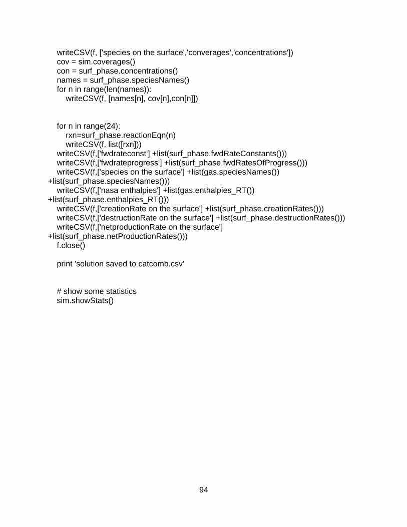
94
writeCSV(f, ['species on the surface','converages','concentrations']) cov = sim.coverages() con = surf_phase.concentrations() names = surf_phase.speciesNames() for n in range(len(names)): writeCSV(f, [names[n], cov[n],con[n]]) for n in range(24): rxn=surf_phase.reactionEqn(n) writeCSV(f, list([rxn])) writeCSV(f,['fwdrateconst'] +list(surf_phase.fwdRateConstants())) writeCSV(f,['fwdrateprogress'] +list(surf_phase.fwdRatesOfProgress())) writeCSV(f,['species on the surface'] +list(gas.speciesNames()) +list(surf_phase.speciesNames())) writeCSV(f,['nasa enthalpies'] +list(gas.enthalpies_RT()) +list(surf_phase.enthalpies_RT())) writeCSV(f,['creationRate on the surface'] +list(surf_phase.creationRates())) writeCSV(f,['destructionRate on the surface'] +list(surf_phase.destructionRates())) writeCSV(f,['netproductionRate on the surface'] +list(surf_phase.netProductionRates())) f.close() print 'solution saved to catcomb.csv' # show some statistics sim.showStats()
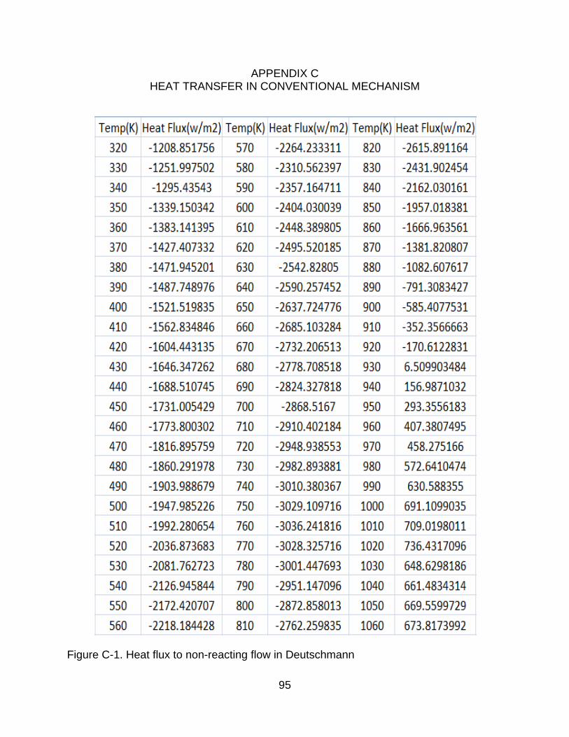
95
APPENDIX C HEAT TRANSFER IN CONVENTIONAL MECHANISM
Figure C-1. Heat flux to non-reacting flow in Deutschmann
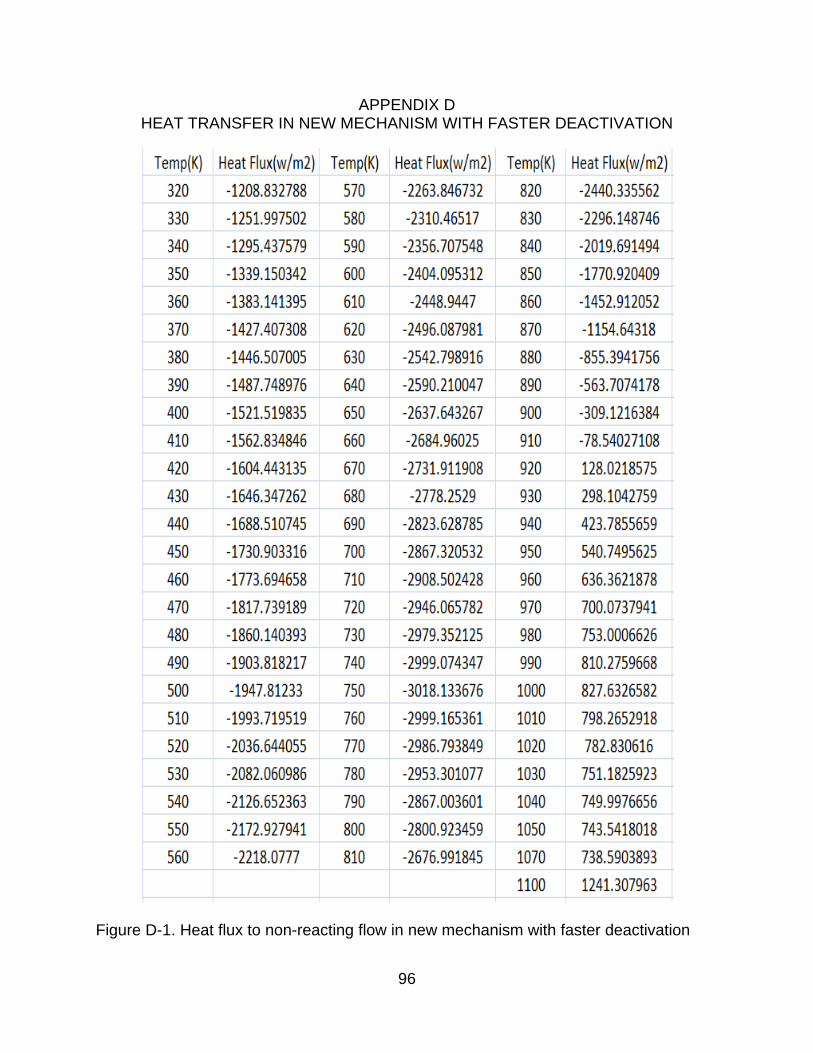
96
APPENDIX D HEAT TRANSFER IN NEW MECHANISM WITH FASTER DEACTIVATION
Figure D-1. Heat flux to non-reacting flow in new mechanism with faster deactivation
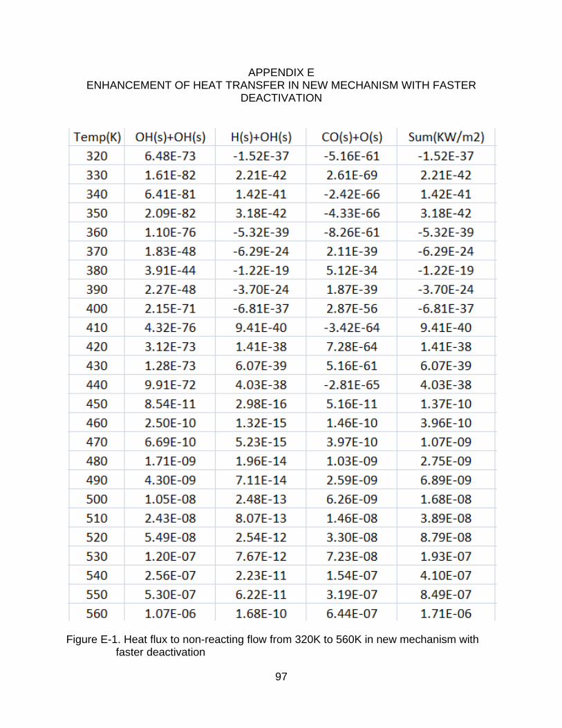
97
APPENDIX E ENHANCEMENT OF HEAT TRANSFER IN NEW MECHANISM WITH FASTER
DEACTIVATION
Figure E-1. Heat flux to non-reacting flow from 320K to 560K in new mechanism with faster deactivation
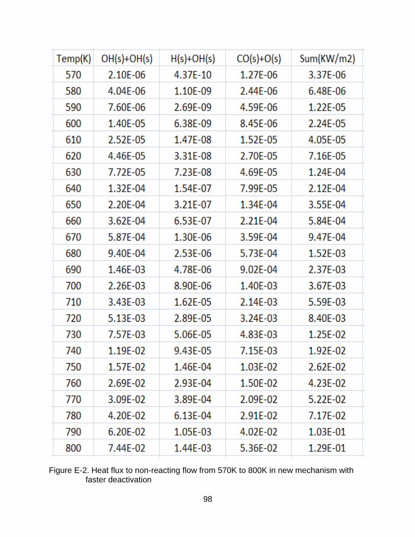
98
Figure E-2. Heat flux to non-reacting flow from 570K to 800K in new mechanism with faster deactivation
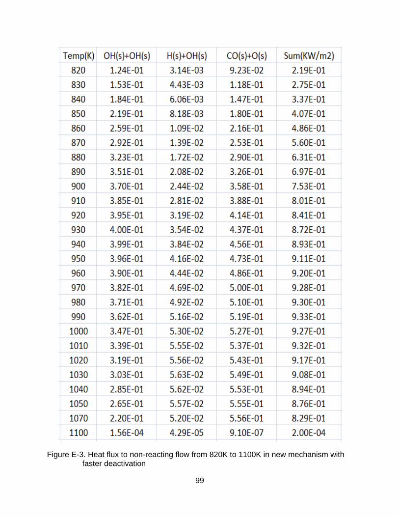
99
Figure E-3. Heat flux to non-reacting flow from 820K to 1100K in new mechanism with faster deactivation
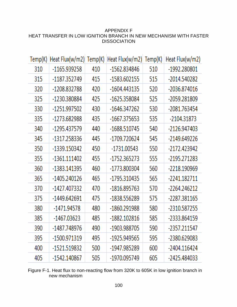
100
APPENDIX F HEAT TRANSFER IN LOW IGNITION BRANCH IN NEW MECHANISM WITH FASTER
DISSOCIATION
Figure F-1. Heat flux to non-reacting flow from 320K to 605K in low ignition branch in new mechanism
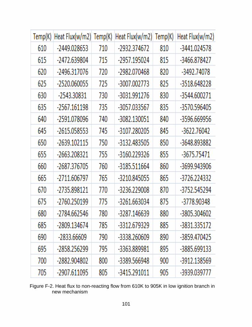
101
Figure F-2. Heat flux to non-reacting flow from 610K to 905K in low ignition branch in new mechanism
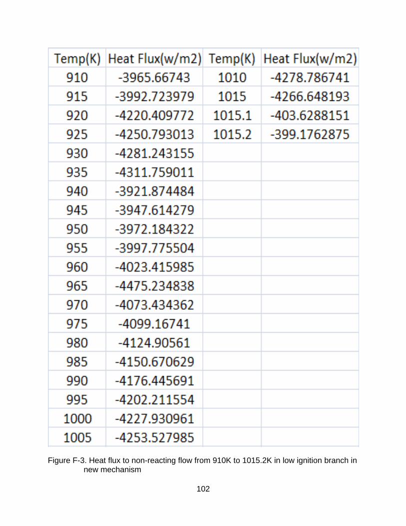
102
Figure F-3. Heat flux to non-reacting flow from 910K to 1015.2K in low ignition branch in new mechanism
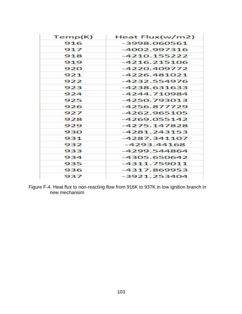
103
Figure F-4. Heat flux to non-reacting flow from 916K to 937K in low ignition branch in new mechanism
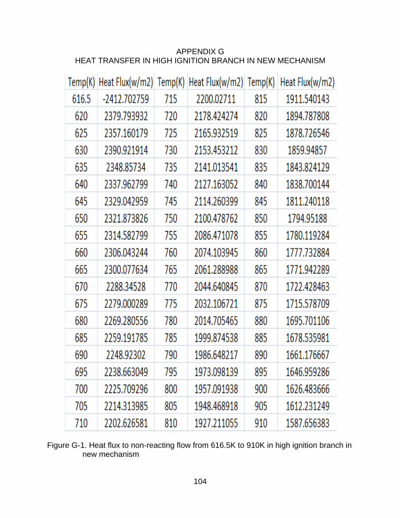
104
APPENDIX G HEAT TRANSFER IN HIGH IGNITION BRANCH IN NEW MECHANISM
Figure G-1. Heat flux to non-reacting flow from 616.5K to 910K in high ignition branch in new mechanism
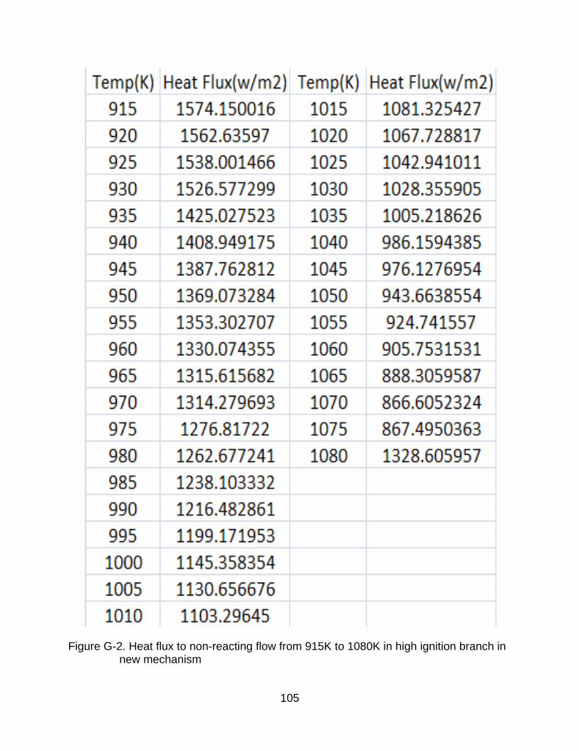
105
Figure G-2. Heat flux to non-reacting flow from 915K to 1080K in high ignition branch in new mechanism
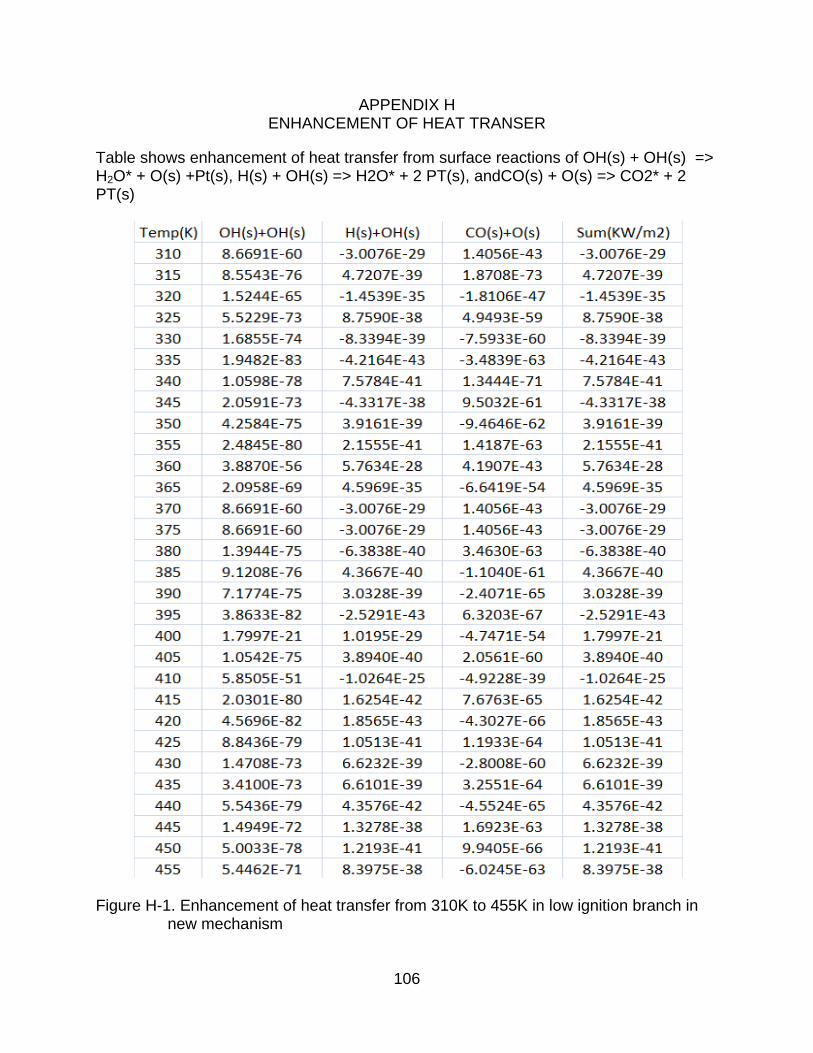
106
APPENDIX H ENHANCEMENT OF HEAT TRANSER
Table shows enhancement of heat transfer from surface reactions of OH(s) + OH(s) => H2O* + O(s) +Pt(s), H(s) + OH(s) => H2O* + 2 PT(s), andCO(s) + O(s) => CO2* + 2 PT(s)
Figure H-1. Enhancement of heat transfer from 310K to 455K in low ignition branch in new mechanism
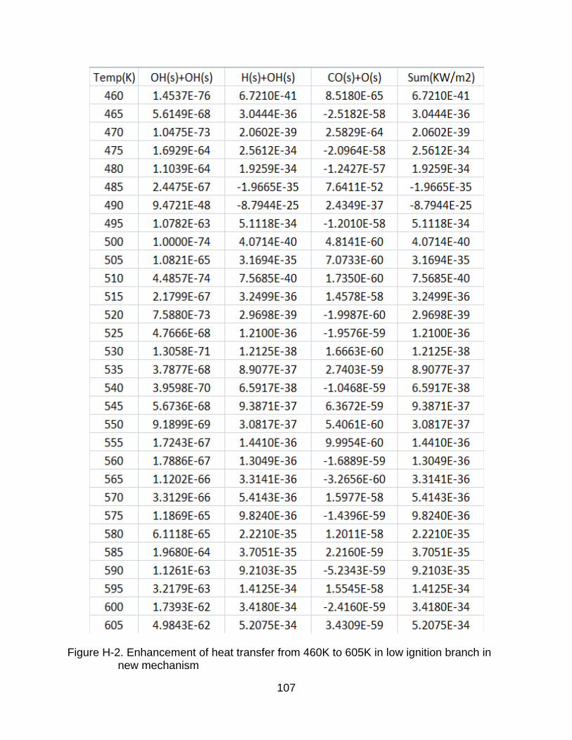
107
Figure H-2. Enhancement of heat transfer from 460K to 605K in low ignition branch in new mechanism
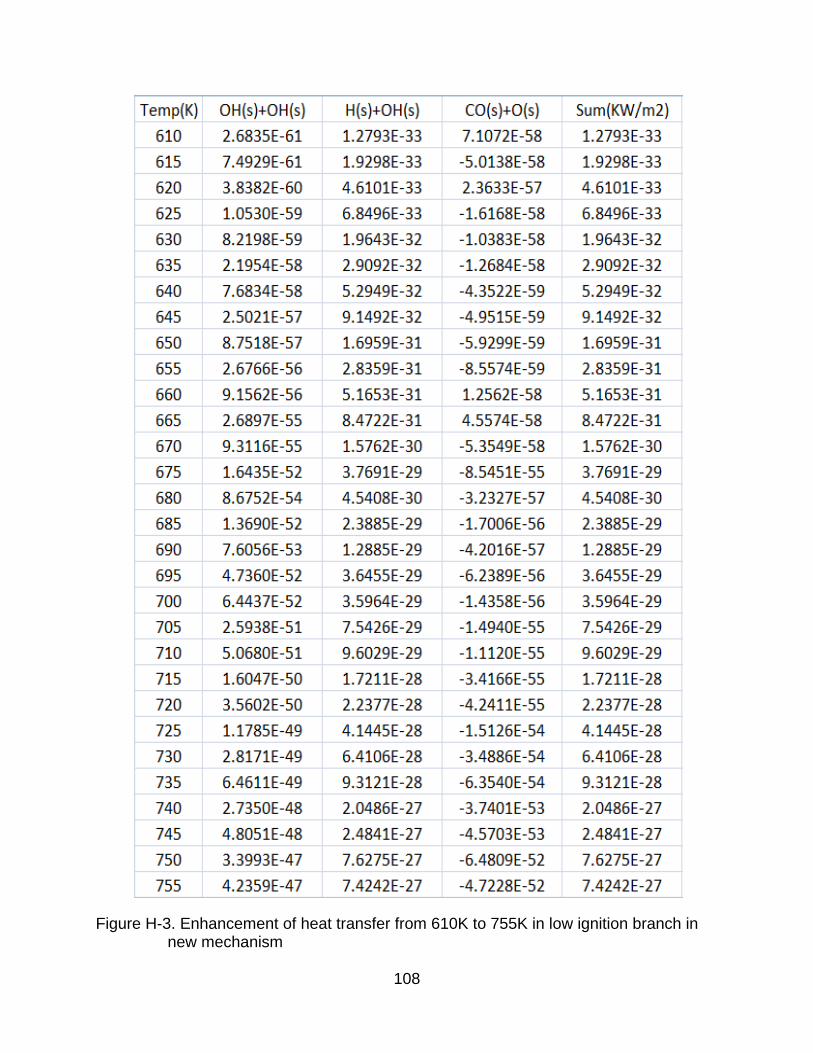
108
Figure H-3. Enhancement of heat transfer from 610K to 755K in low ignition branch in new mechanism
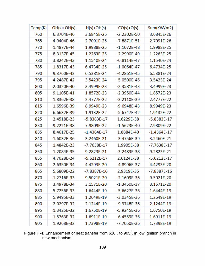
109
Figure H-4. Enhancement of heat transfer from 610K to 905K in low ignition branch in new mechanism
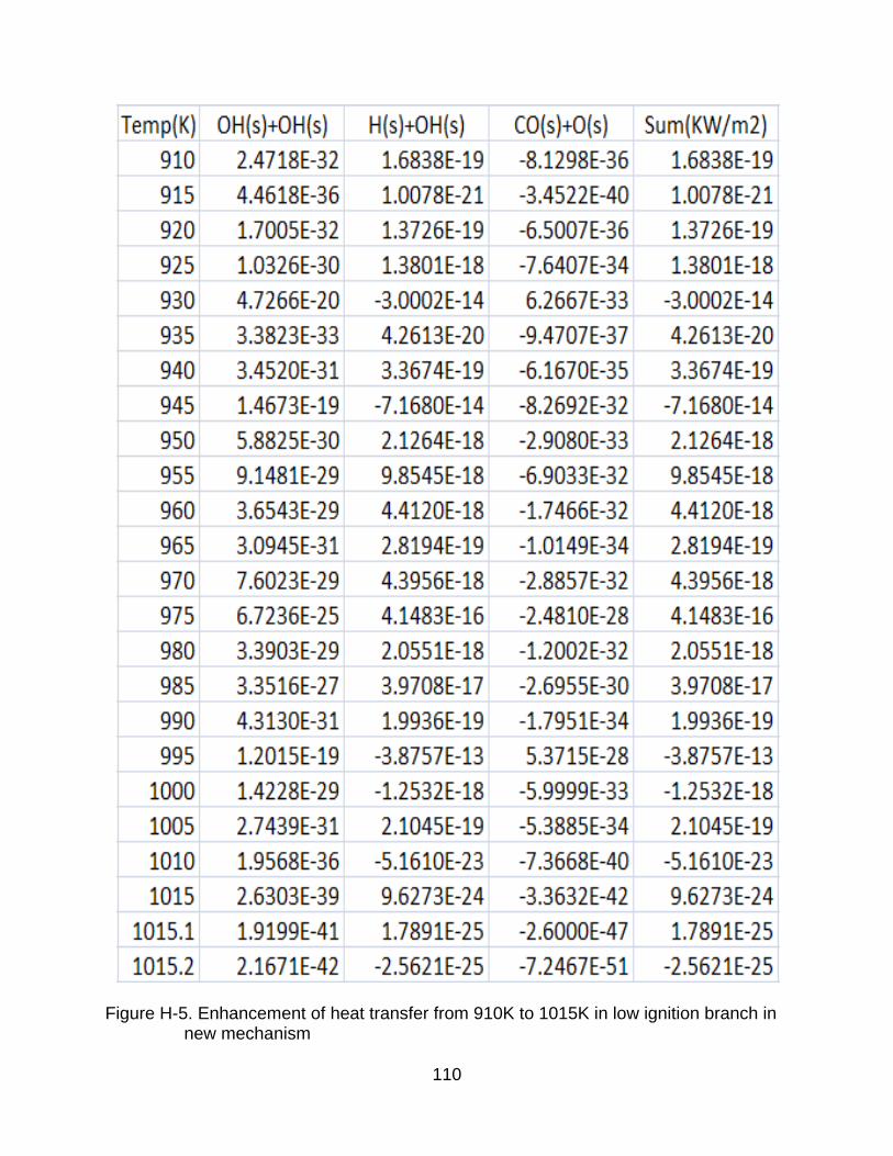
110
Figure H-5. Enhancement of heat transfer from 910K to 1015K in low ignition branch in new mechanism
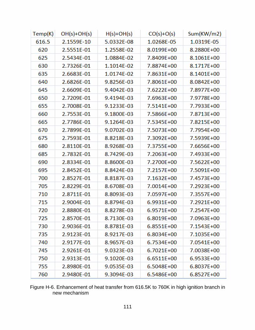
111
Figure H-6. Enhancement of heat transfer from 616.5K to 760K in high ignition branch in new mechanism
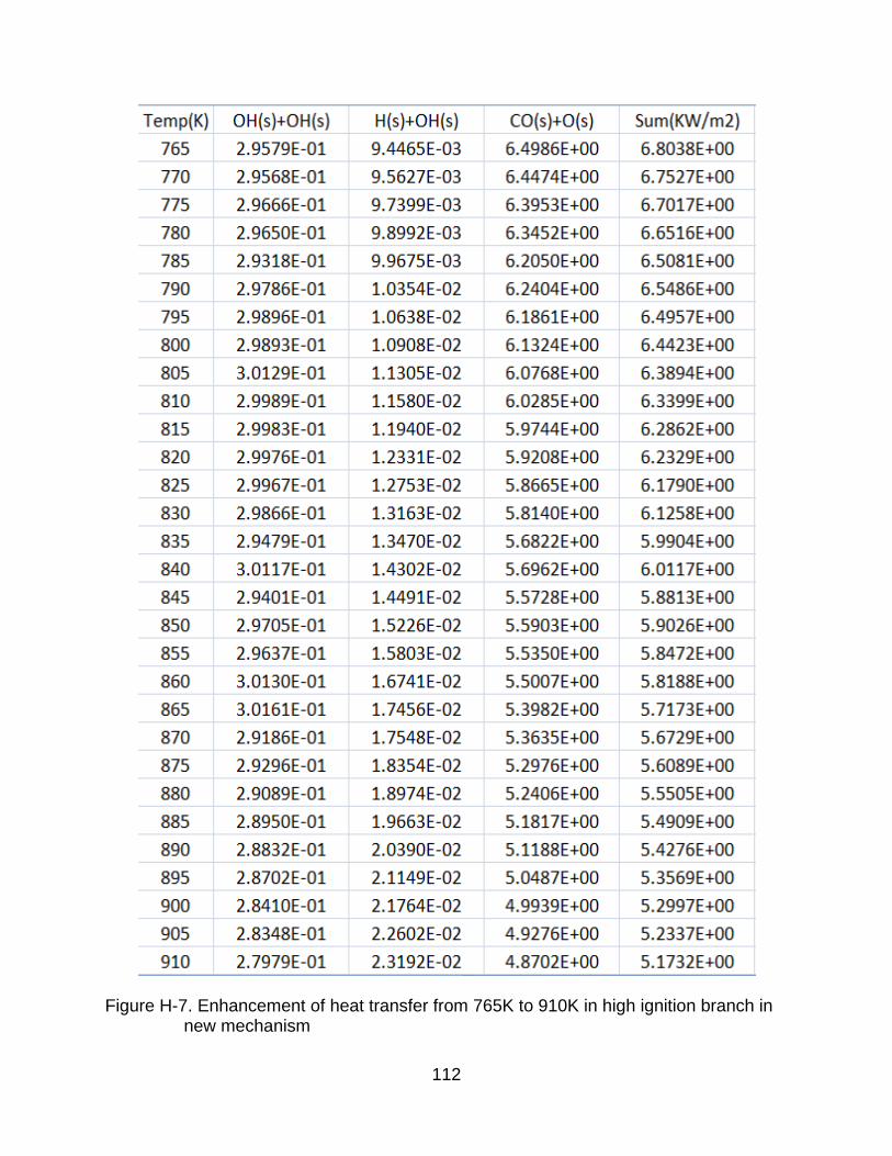
112
Figure H-7. Enhancement of heat transfer from 765K to 910K in high ignition branch in new mechanism
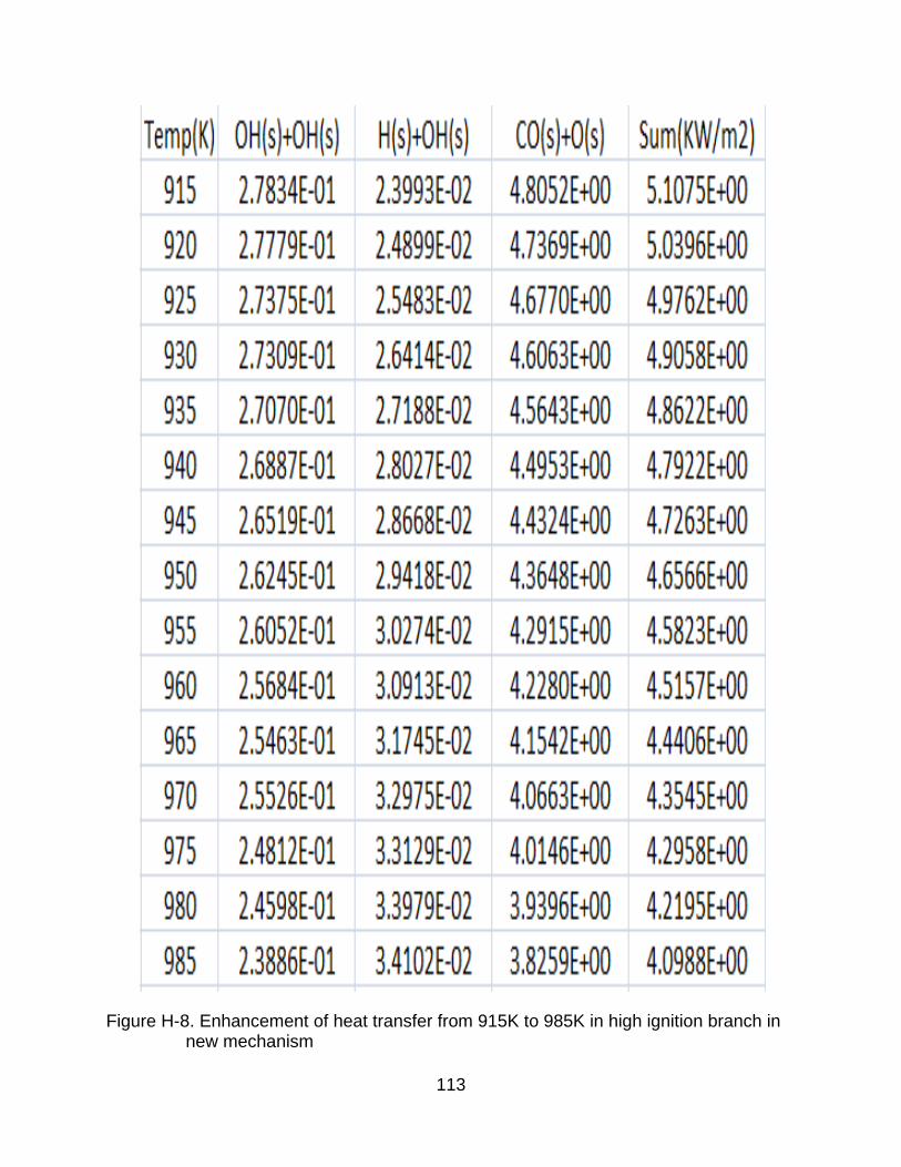
113
Figure H-8. Enhancement of heat transfer from 915K to 985K in high ignition branch in new mechanism
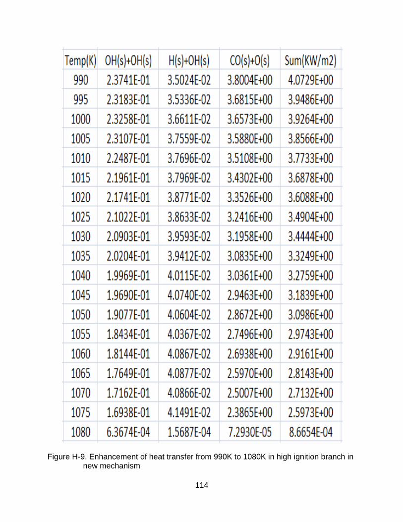
114
Figure H-9. Enhancement of heat transfer from 990K to 1080K in high ignition branch in new mechanism
115
LIST OF REFERENCES
[1] Deutschmann, O., Behrendt, F., and Warnatz, J., "Formal treatment of catalytic combustion and catalytic conversion of methane", Catalysis Today, Vol 46,1998, pp.155-163 [2] Deutschmann, O., Behrendt, F., and Warnatz J., "Modelling and simulation of heterogeneous oxidation of methane on a platinum foil", Catalysis Today, Vol 21,1994, pp.461-470 [3] Deutschmann, O., Maier, L.I., Riedel, U., Stroemman, A.H., and Dibble, R.W, "Hydrogen assisted catalytic combustion of methane on platinum", Catalysis Today , Vol 59, 2000, pp.141-150 [4] Moallemi, F., Batley, G., Dupont, V., Foster, T.J., Pourkashanian, M., and Williams, A., "Chemical modelling and measurements of the catalytic combustion of CH4/air mixture on platinam and palladium catalysts", Catalysis Today, Vol 47, 1999, pp.235-244 [5] Henry, C.A., Mikolaitis, W., Szedlacsek, P., and Hahn, D.W., "Investigation of Heat Transfer under Catalytic Combustion of Methane: Effect of Heterogeneous Chemistry on Heat Transfer Enhancement" [6] Williams, W.R., Stenzel, M.T., sing, X. and Schmidt, L.D., "Bifurcation behavior in homogeneous-heterogeneous combustion: I. Experimental results over platinum" Combust and Flame, Vol 84, 1991, pp.277-291 [7] Kuo, K.K.(2005), Principles of Combustion, Second Edition, Hoboken, New Jersey, John Wiley & Sons [8] McCash, E.M.(2001), Surface Chemistry, Oxford, New York, Oxford University Press [9] Hayes, R.E. and Kolaczkowski, S.T.(1997), Introduction to Catalytic Combustion, Amsterdam, Netherlands, Gordon and Breach Science [10] Frenklach, M., Bowman, T., Smith, G., and Gardiner, B., "GRI Mech", 2000, Gas Research Institute, http://www.me.berkeley.edu/gri-mech/, July 2011 [11] Deutschmann, O., "Surface Mechanism of the CH4-O2 Reactions on Platinum", 1995, Heidelberg University, http://www.detchem.com/mechanisms.html, July 2011 [12] Wikipedia, "Methane", Wikipedia, http://en.wikipedia.org/wiki/Methane, July 2011 [13] Wikipedia, "Catalysis", Wikipedia, http://en.wikipedia.org/wiki/Catalysis, July 2011
116
[14] Martin, K.K., and Rachul, L., "NASA Glenn Tests Alternative Green Rocket Engine", 2010, http://www.nasa.gov/centers/glenn/news/pressrel/2010/10-049_green.html, July 2011 [15] Goodwin, D.G., "Defining Phases and Interfaces, Cantera 1.5", Division of Engineering and Applied Science, California Institute of Technology, August 14, 2003 [16] Goodwin, D.G., "Cantera User's Guide Fortran Version Release 1.2", Division of Engineering and Applied Science, California Institute of Technology, November, 2001 [17] Goodwin, D.G., "CANTERA", Division of Engineering and Applied Science, California Institute of Technology
117
BIOGRAPHICAL SKETCH
Sungsik Kim was born in Seoul, Korea in 1983. He majored in nuclear engineering
Kyung Hee University and received a Bachelor of Engineering degree in nuclear
engineering in 2008. He switched to mechanical and aerospace engineering in 2009
when he attended University of Florida, Gainesville. He received a Master of Science
degree in mechanical and aerospace engineering in 2011. His research interests are
catalytic combustion, combustion process and emission control, and alternative fuel
engines.