Heat transfer chapter 2 solutions

7/27/2019 Heat transfer chapter 2 solutions

http://slidepdf.com/reader/full/heat-transfer-chapter-2-solutions 1/13

PROBLEM 2.12

KNOWN: Plane wall with prescribed thermal conductivity, thickness, and surface temperatures.

FIND: Heat flux, q x , and temperature gradient, dT/dx, for the three different coordinate systems

shown.SCHEMATIC:

ASSUMPTIONS: (1) One-dimensional heat flow, (2) Steady-state conditions, (3) No internal

generation, (4) Constant properties.

ANALYSIS: The rate equation for conduction heat transfer is

q k dT

dxx , (1)

where the temperature gradient is constant throughout the wall and of the form

T L T 0dT.

dx L

(2)

Substituting numerical values, find the temperature gradients,

(a) 2 1 600 400 K dT T T

2000 K/mdx L 0.100m

<

(b) 1 2 400 600 K dT T T

2000 K/mdx L 0.100m

<

(c) 2 1 600 400 K dT T T

2000 K/m.dx L 0.100m

<

The heat rates, using Eq. (1) with k = 100 W/mK, are

(a) 2x

Wq 100 2000 K/m=-200 kW/m

m K

<

(b) 2x

Wq 100 ( 2000 K/m)=+200 kW/m

m K

<

(c)

q W

m K K / m = -200 kW/ mx

2100 2000 <



PROBLEM 2.28

KNOWN: Steady-state temperature distribution in a cylindrical rod having uniform heat generation

of & .q W / m13= ×5 107

FIND: (a) Steady-state centerline and surface heat transfer rates per unit length, ′q r . (b) Initial time

rate of change of the centerline and surface temperatures in response to a change in the generation rate

from

8 3

1 2q to q = 10 W/m .& &

SCHEMATIC:

ASSUMPTIONS: (1) One-dimensional conduction in the r direction, (2) Uniform generation, and (3)

Steady-state for & .q = 5 10 W / m17 3×

ANALYSIS: (a) From the rate equations for cylindrical coordinates,

′′ = −q k T

r q = -kA

T

r r r

∂

∂

∂

∂ .

Hence,

( )r T

q k 2 rL r

∂ π

∂ = −

or

′ = −q kr

T

r r 2π

∂

∂ (1)

where ∂T/∂r may be evaluated from the prescribed temperature distribution, T(r).

At r = 0, the gradient is (∂T/∂r) = 0. Hence, from Equation (1) the heat rate is

( )r q 0 0.′ = <

At r = r o, the temperature gradient is

( ) ( )( )o

o

5 5o2

r=r

5

r=r

T K 2 4.167 10 r 2 4.167 10 0.025m

r m

T 0.208 10 K/m. r

∂

∂

∂ ∂

⎡ ⎤⎤= − × = − ×⎢ ⎥⎥⎦ ⎣ ⎦

⎤ = − ×⎥⎦

Continued …..



PROBLEM 2.28 (Cont.)

Hence, the heat rate at the outer surface (r = r o) per unit length is

( ) [ ]( ) 5r oq r 2 30 W/m K 0.025m 0.208 10 K/mπ ⎡ ⎤′ = − ⋅ − ×⎢ ⎥⎣ ⎦

( ) 5r oq r 0.980 10 W/m.′ = × <

(b) Transient (time-dependent) conditions will exist when the generation is changed, and for the

prescribed assumptions, the temperature is determined by the following form of the heat equation,

Equation 2.26

2 p1 T T

kr q cr r r t

∂ ∂ ∂ ρ

∂ ∂ ∂

⎡ ⎤+ =⎢ ⎥⎣ ⎦

&

Hence

2 p

T 1 1 T kr q .

t c r r r

∂ ∂ ∂

∂ ρ ∂ ∂

⎡ ⎤⎡ ⎤= +⎢ ⎥⎢ ⎥⎣ ⎦⎣ ⎦

&

However, initially (at t = 0), the temperature distribution is given by the prescribed form, T(r) = 800 -

4.167×105r 2, and

( )51 T k kr r -8.334 10 r

r r r r r

∂ ∂ ∂

∂ ∂ ∂

⎡ ⎤ ⎡ ⎤= × ⋅⎢ ⎥ ⎢ ⎥⎣ ⎦⎣ ⎦

( )5k 16.668 10 r

r = − × ⋅

5 230 W/m K -16.668 10 K/m⎡ ⎤= ⋅ ×⎢ ⎥⎣ ⎦

( )7 315 10 W/m the original q=q .= − × & &

Hence, everywhere in the wall,

7 8 33

T 15 10 10 W/m

t 1100 kg/m 800 J/kg K

∂

∂ ⎡ ⎤= − × +⎢ ⎥⎣ ⎦× ⋅

or

∂

∂

T

t K / s.= 5682. <

COMMENTS: (1) The value of (∂T/∂t) will decrease with increasing time, until a new steady-state

condition is reached and once again (∂T/∂t) = 0. (2) By applying the energy conservation requirement,

Equation 1.12c, to a unit length of the rod for the steady-state condition, & & .′ − ′ + ′ =E E Ein out gen 0

Hence ( ) ( ) ( )2r r o 1 oq 0 q r q r .π ′ ′− = − &



PROBLEM 2.34

KNOWN: Steady-state conduction with uniform internal energy generation in a plane wall;temperature distribution has quadratic form. Surface at x=0 is prescribed and boundary at x = L is

insulated.

FIND: (a) Calculate the internal energy generation rate, q , by applying an overall energy balance to

the wall, (b) Determine the coefficients a, b, and c, by applying the boundary conditions to the

prescribed form of the temperature distribution; plot the temperature distribution and label as Case 1,(c) Determine new values for a, b, and c for conditions when the convection coefficient is halved, and

the generation rate remains unchanged; plot the temperature distribution and label as Case 2; (d)Determine new values for a, b, and c for conditions when the generation rate is doubled, and the

convection coefficient remains unchanged (h = 500 W/m2

K); plot the temperature distribution and

label as Case 3.

SCHEMATIC:

x L = 50 mm

Insulatedboundary

h = 500 W/m -K2 Fluid

T = 20 Cooo

T(0) = T = 120 Coo

T(x) = a + bx + cx2

k = 5 W/m-K, q.

ASSUMPTIONS: (1) Steady-state conditions, (2) One-dimensional conduction with constant

properties and uniform internal generation, and (3) Boundary at x = L is adiabatic.

ANALYSIS: (a) The internal energy generation rate can be calculated from an overall energy balanceon the wall as shown in the schematic below.

in out gen in convE E E 0 where E q

oh T T q L 0 (1)

2 6 3oq h T T / L 500 W / m K 20 120 C / 0.050 m 1.0 10 W / m <

T , hoo

q (0)x” q (L)x”

x

x

L

x = L

To To

(a) Overall energy balance (b) Surface energy balances

.

Egen“

convq” conv

q”k, q.

(b) The coefficients of the temperature distribution, T(x) = a + bx + cx2

, can be evaluated by applying

the boundary conditions at x = 0 and x = L. See Table 2.2 for representation of the boundary

conditions, and the schematic above for the relevant surface energy balances.

Boundary condition at x = 0, convection surface condition

in out conv x xx 0

dTE E q q 0 0 where q 0 k

dx

ox 0

h T T k 0 b 2cx 0

Continued ...




2 4o b h T T / k 500 W / m K 20 120 C / 5 W / m K 1.0 10 K / m (2)<

Boundary condition at x = L, adiabatic or insulated surface

in out x xx L

dTE E q L 0 where q L k

dx

x L

k 0 b 2cx 0

(3)

4 5 2c b / 2L 1.0 10 K / m / 2 0.050m 1.0 10 K / m <

Since the surface temperature at x = 0 is known, T(0) = To = 120C, find

T 0 120 C a b 0 c 0 or a 120 C (4)<

Using the foregoing coefficients with the expression for T(x) in the Workspace of IHT, thetemperature distribution can be determined and is plotted as Case 1 in the graph below.

(c) Consider Case 2 when the convection coefficient is halved, h2 = h/2 = 250 W/m2

K, 6

q 1 10

W/m3

and other parameters remain unchanged except that oT 120 C. We can determine a, b, and c

for the temperature distribution expression by repeating the analyses of parts (a) and (b).

Overall energy balance on the wall, see Eqs. (1,4)

6 3 2oa T q L/ h T 1 10 W / m 0.050m / 250 W / m K 20 C 220 C <

Surface energy balance at x = 0, see Eq. (2)

2 4o b h T T / k 250 W / m K 20 220 C / 5 W / m K 1.0 10 K / m <

Surface energy balance at x = L, see Eq. (3)

4 5 2c b / 2L 1.0 10 K / m / 2 0.050m 1.0 10 K / m <

The new temperature distribution, T2 (x), is plotted as Case 2 below.

(d) Consider Case 3 when the internal energy volumetric generation rate is doubled,

6 33q 2q 2 10 W / m , h = 500 W/m

2K, and other parameters remain unchanged except that

oT 120 C. Following the same analysis as part (c), the coefficients for the new temperature

distribution, T (x), are

4 5 2a 220 C b 2 10 K / m c 2 10 K / m <

and the distribution is plotted as Case 3 below.

Continued …




COMMENTS: Note the following features in the family of temperature distributions plotted above.The temperature gradients at x = L are zero since the boundary is insulated (adiabatic) for all cases.

The shapes of the distributions are all quadratic, with the maximum temperatures at the insulated boundary.

By halving the convection coefficient for Case 2, we expect the surface temperature To to increase

relative to the Case 1 value, since the same heat flux is removed from the wall qL but the

convection resistance has increased.

By doubling the generation rate for Case 3, we expect the surface temperature To to increase relative

to the Case 1 value, since double the amount of heat flux is removed from the wall 2qL .

Can you explain why To is the same for Cases 2 and 3, yet the insulated boundary temperatures are

quite different? Can you explain the relative magnitudes of T(L) for the three cases?

0 5 10 15 20 25 30 35 40 45 50

Wall position, x (mm)

100

200

300

400

500

600

700

800

T e m p e r a t u r e ,

T ( C )

1. h = 500 W/m^2.K, qdot = 1e6 W/m^32. h = 250 W/m^2.K, qdot = 1e6 W/m^33. h = 500 W/m^2.K, qdot = 2e6 W/m^3



PROBLEM 2.49

KNOWN: Steady-state temperature distribution for hollow cylindrical solid with volumetric heat

generation.

FIND: (a) Determine the inner radius of the cylinder, r i, (b) Obtain an expression for the volumetric

rate of heat generation, q, (c) Determine the axial distribution of the heat flux at the outer surface,

r oq r ,, z and the heat rate at this outer surface; is the heat rate in or out of the cylinder; (d)

Determine the radial distribution of the heat flux at the end faces of the cylinder, z oq r, z and

z oq r, z , and the corresponding heat rates; are the heat rates in or out of the cylinder; (e)

Determine the relationship of the surface heat rates to the heat generation rate; is an overall energy balance satisfied?

SCHEMATIC:

boundary

Insulated a = 20oC

b = 150 C/mo 2

k = 16 W/m-K

c = -12 Co

d = -300 C/mo 2

T(r,z) = a + br + cln(r) + dz r(m), z(m)2 2

+z = 2.5 mo

-z = 2.5 mo

z

r r i0 r = 1 mo

ASSUMPTIONS: (1) Steady-state conditions, (2) Two-dimensional conduction with constant properties and volumetric heat generation.

ANALYSIS: (a) Since the inner boundary, r = r i, is adiabatic, then r iq r z 0., Hence the

temperature gradient in the r-direction must be zero.

i ir i

T0 2br c / r 0 0

r

1/ 21/ 2

i 2

c 12 Cr 0.2 m

2b 2 150 C / m

<

(b) To determine q, substitute the temperature distribution into the heat diffusion equation, Eq. 2.26,

for two-dimensional (r,z), steady-state conduction

1 T T qr 0

r r r z z k

1 q

r 0 2br c / r 0 0 0 0 2dz 0r r z k

1 q

4br 0 2d 0r k

2 2 3q k 4b 2d 16 W / m K 4 150 C / m 2 300 C / m 0W / m

<

(c) The heat flux and the heat rate at the outer surface, r = r o, may be calculated using Fourier’s law.

r o, o o

r o

Tq r z k k 0 2br c / r 0

r

Continued …




2 2

r o,q r z 16 W / m K 2 150 C / m 1 m 12 C /1 m 4608 W / m <

o r r o, r o oq r A q r z where A 2 r 2z

2

r oq r 4 1 m 2.5 m 4608 W / m 144, 765 W <

Note that the sign of the heat flux and heat rate in the positive r-direction is negative, and hence theheat flow is into the cylinder.

(d) The heat fluxes and the heat rates at end faces, z = + zo and – zo, may be calculated using Fourier’s

law. The direction of the heat rate in or out of the end face is determined by the sign of the heat flux inthe positive z-direction.

At the upper end face, z = + zo: <

o

z o oz

Tq r, z k k 0 0 0 2dz

z

2 2z oq r, z 16 W / m K 2 300 C / m 2.5 m 24, 000 W / m <

2 2z o z z o z o iq z A q r, z where A r r

2 2 2 2z oq z 1 0.2 m 24, 000 W / m 72, 382 W <

Thus, heat flows out of the cylinder.

At the lower end face, z = - zo: <

z o o

zo

Tq r, z k k 0 0 0 2d( z

z)

2 2

z oq r, z 16 W / m K 2 300 C / m 2.5 m 24, 000 W / m <

z oq z 72, 382 W <

Again, heat flows out of the cylinder.

(e) The heat rates from the surfaces and the volumetric heat generation can be related through anoverall energy balance on the cylinder as shown in the sketch.

r

r q”(r ,z) = -4,608 W/m2

o

z

z

z

z

q”(r,-z ) = -24,000 W/mo 2

q”(r,+z ) = +24,000 W/mo

q (r,-z ) = -72,382 Wo

q (r,+z ) = +72,382 Wo

q ( ) = -144,765 Wr ,zo

z

r

Continued…




in out gen genE E E 0 where E q 0

in r oE q r 144, 765 W 144, 765 W <

out z o z oE q z q z 72, 382 72, 382 W 144, 764 W <

The overall energy balance is satisfied.

COMMENTS: When using Fourier’s law, the heat flux zq denotes the heat flux in the positive z-

direction. At a boundary, the sign of the numerical value will determine whether heat is flowing into

or out of the boundary.



PROBLEM 2.52

KNOWN: Spherical container with an exothermic reaction enclosed by an insulating material whose

outer surface experiences convection with adjoining air and radiation exchange with large

surroundings.

FIND: (a) Verify that the prescribed temperature distribution for the insulation satisfies the

appropriate form of the heat diffusion equation; sketch the temperature distribution and label key

features; (b) Applying Fourier's law, verify the conduction heat rate expression for the insulation layer,q r , in terms of Ts,1 and Ts,2; apply a surface energy balance to the container and obtain an alternative

expression for q r in terms of q & and r 1; (c) Apply a surface energy balance around the outer surface of

the insulation to obtain an expression to evaluate Ts,2; (d) Determine Ts,2 for the specified geometry

and operating conditions; (e) Compute and plot the variation of Ts,2 as a function of the outer radius

for the range 201 ≤ r 2 ≤ 210 mm; explore approaches for reducing Ts,2 ≤ 45°C to eliminate potential

risk for burn injuries to personnel.

SCHEMATIC:

ASSUMPTIONS: (1) One-dimensional, radial spherical conduction, (2) Isothermal reaction in

container so that To = Ts,1, (2) Negligible thermal contact resistance between the container and

insulation, (3) Constant properties in the insulation, (4) Surroundings large compared to the insulated

vessel, and (5) Steady-state conditions.

ANALYSIS: The appropriate form of the heat diffusion equation (HDE) for the insulation follows

from Eq. 2.29,

2

2

1 d dTr 0

dr dr r =

⎛ ⎞⎜ ⎟⎝ ⎠

(1) <

The temperature distribution is given as

( ) ( ) ( )

( )1

s,1 s,1 s,21 2

1 r r T r T T T

1 r r

−= − −

−

⎡ ⎤⎢ ⎥⎣ ⎦

(2)

Substitute T(r) into the HDE to see if it is satisfied:

( ) ( )

( )

21

2 s,1 s,221 2

0 r r 1 d

r 0 T T 0dr 1 r r r

+

− − =−

⎛ ⎞⎡ ⎤⎜ ⎟⎢ ⎥⎜ ⎟⎢ ⎥⎜ ⎟⎢ ⎥⎣ ⎦⎝ ⎠

( )( )

1s,1 s,22

1 2

r 1 d T T 0

dr 1 r r r + − =

−

⎛ ⎞⎜ ⎟⎝ ⎠

<

and since the expression in parenthesis is independent of r, T(r) does indeed satisfy the HDE. The

temperature distribution in the insulation and its key features are as follows:

Continued...




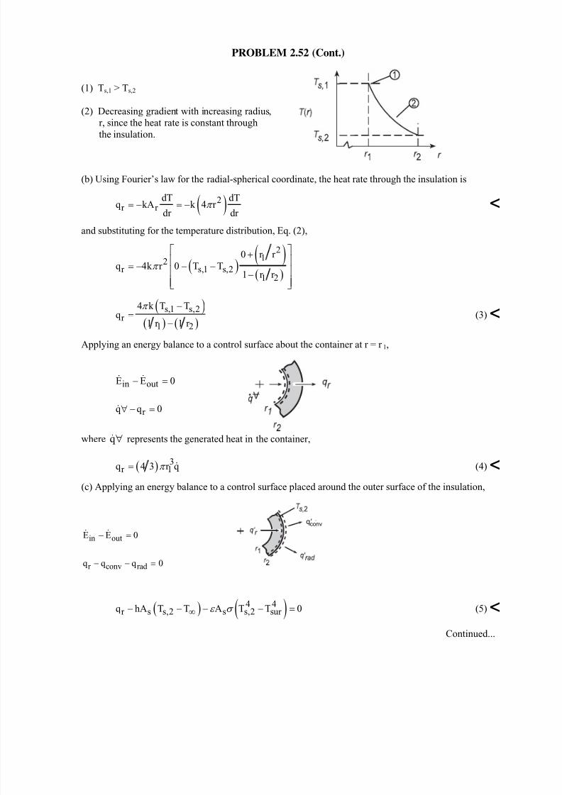
(1) Ts,1 > Ts,2

(2) Decreasing gradient with increasing radius,

r, since the heat rate is constant through

the insulation.

(b) Using Fourier’s law for the radial-spherical coordinate, the heat rate through the insulation is

( )2r r

dT dTq kA k 4 r

dr dr π = − = − <

and substituting for the temperature distribution, Eq. (2),

( ) ( )

( )

212

r s,1 s,2

1 2

0 r r

q 4k r 0 T T

1 r r

+= − − −

−

⎡ ⎤⎢ ⎥⎢ ⎥⎢ ⎥⎣ ⎦

π

( )( ) ( )

s,1 s,2r

1 2

4 k T Tq

1 r 1 r

π −=

− (3) <

Applying an energy balance to a control surface about the container at r = r 1,

in outE E 0− =& &

r q q 0∀ − =&

where q ∀& represents the generated heat in the container,

( ) 3r 1q 4 3 r q π = & (4) <

(c) Applying an energy balance to a control surface placed around the outer surface of the insulation,

in outE E 0− =& &

r conv rad q q q 0− − =

( ) ( )4 4r s s,2 s s,2 sur q hA T T A T T 0ε σ ∞− − − − = (5) <

Continued...

′convq




where

2s 2A 4 r π = (6)

These relations can be used to determine Ts,2 in terms of the variables q & , r 1, r 2, h, T∞ , ε and Tsur .

(d) Consider the reactor system operating under the following conditions:

r 1 = 200 mm h = 5 W/m2⋅K ε = 0.9

r 2 = 208 mm T∞ = 25°C Tsur = 35°C

k = 0.05 W/m⋅K

The heat generated by the exothermic reaction provides for a volumetric heat generation rate,

( ) 3o o oq q exp A T q 5000 W m A 75K = − = =& & (7)

where the temperature of the reaction is that of the inner surface of the insulation, To = Ts,1. The

following system of equations will determine the operating conditions for the reactor.

Conduction rate equation, insulation, Eq. (3),

( )( )

s,1 s,2r

4 0.05 W m K T Tq

1 0.200 m 1 0.208 m

π × ⋅ −=

− (8)

Heat generated in the reactor, Eqs. (4) and (7),

( )3r q 4 3 0.200 m q π = & (9)

( )3s,1q 5000 W m exp 75 K T= −& (10)

Surface energy balance, insulation, Eqs. (5) and (6),

( ) ( )( )42 8 2 4 4r s s,2 s s,2q 5 W m K A T 298 K 0.9A 5.67 10 W m K T 308 K 0

−− ⋅ − − × ⋅ − = (11)

( )2sA 4 0.208 mπ = (12)

Solving these equations simultaneously, find that

s,1 s,2T 94.3 C T 52.5 C= =o o <

That is, the reactor will be operating at To = Ts,1 = 94.3°C, very close to the desired 95°C operating

condition.

(e) Using the above system of equations, Eqs. (8)-(12), we have explored the effects of changes in the

convection coefficient, h, and the insulation thermal conductivity, k, as a function of insulation

thickness, t = r 2 - r 1.

Continued...




0 2 4 6 8 10

Insulation thickness, (r2 - r1) (mm)

35

40

45

50

55

O u t e r s u r f a c e t e m p e r a t u r e , T s 2 ( C )

k = 0.05 W/m.K, h = 5 W/m^2.K

k = 0.01 W/m.K, h = 5 W/m^2.Kk = 0.05 W/m.K, h = 15 W/m^2.K

0 2 4 6 8 10

Insulation thickness, (r2-r1) (mm)

20

40

60

80

100

120

R e a c t i o n t e m p e r a t u r e ,

T o ( C )

k = 0.05 W/m.K, h = 5 W/m^2.K

k = 0.01 W/m.K, h = 5 W/m^2.Kk = 0.05 W/m.K, h = 15 W/m^2.K

In the Ts,2 vs. (r 2 - r 1) plot, note that decreasing the thermal conductivity from 0.05 to 0.01 W/m⋅Kslightly increases Ts,2 while increasing the convection coefficient from 5 to 15 W/m2⋅K markedly

decreases Ts,2. Insulation thickness only has a minor effect on Ts,2 for either option. In the To vs. (r 2 -

r 1) plot, note that, for all the options, the effect of increased insulation is to increase the reaction

temperature. With k = 0.01 W/m⋅K, the reaction temperature increases beyond 95°C with less than 2

mm insulation. For the case with h = 15 W/m2⋅K, the reaction temperature begins to approach 95°C

with insulation thickness around 10 mm. We conclude that by selecting the proper insulation

thickness and controlling the convection coefficient, the reaction could be operated around 95°C suchthat the outer surface temperature would not exceed 45°C.

Heat transfer chapter 2 solutions

Documents

Transcript of Heat transfer chapter 2 solutions