Heat kernels on metric spaces with doubling measuregrigor/survey.pdf · Heat kernels on metric...
32
Heat kernels on metric spaces with doubling measure Alexander Grigor’yan, Jiaxin Hu and Ka-Sing Lau Abstract. In this survey we discuss heat kernel estimates of self-similar type on metric spaces with doubling measures. We characterize the tail functions from heat kernel estimates in both non-local and local cases. In the local case we also specify the domain of the energy form as a certain Besov space, and identify the walk dimension in terms of the critical Besov exponent. The techniques used include self-improvement of heat kernel upper bound and the maximum principle for weak solutions. All proofs are completely analytic. Mathematics Subject Classification (2000). Primary: 47D07, Secondary: 28A80, 46E35. Keywords. Doubling measure, heat kernel, maximum principle, heat equation. Contents 1. Introduction 2 2. What is a heat kernel 2 2.1. The notion of a heat kernel 2 2.2. Heat semigroup and Dirichlet forms 3 2.3. Examples 6 3. Auxiliary material on metric measure spaces 7 3.1. Besov spaces 8 3.2. Doubling condition and reverse doubling condition 8 4. Consequences of heat kernel estimates 10 4.1. Consequences of lower bound 10 4.2. Consequences of upper bound 13 4.3. Walk dimension 16 4.4. Consequence of two-sided estimates (non-local case) 17 5. A maximum principle and its applications 17 5.1. Weak differentiation 17 5.2. Maximum principle for weak solutions 19 5.3. Some applications of the maximum principle 20 6. Upper bounds in the local case 22 6.1. Exponential tail 22 6.2. Consequences of two-sided estimates (local case) 27 References 31 AG was supported by SFB 701 of the German Research Council (DFG) and the Grants from the Department of Mathematics and IMS in CUHK. JH was supported by NSFC (Grant No. 10631040) and the HKRGC Grant in CUHK. KSL was supported by the HKRGC Grant in CUHK.
Transcript of Heat kernels on metric spaces with doubling measuregrigor/survey.pdf · Heat kernels on metric...
Heat kernels on metric spaces with doubling measure
Alexander Grigor’yan, Jiaxin Hu and Ka-Sing Lau
Abstract. In this survey we discuss heat kernel estimates of self-similar type on metric spaceswith doubling measures. We characterize the tail functions from heat kernel estimates in bothnon-local and local cases. In the local case we also specify the domain of the energy form as acertain Besov space, and identify the walk dimension in terms of the critical Besov exponent.The techniques used include self-improvement of heat kernel upper bound and the maximumprinciple for weak solutions. All proofs are completely analytic.
Mathematics Subject Classification (2000). Primary: 47D07, Secondary: 28A80, 46E35.
Keywords. Doubling measure, heat kernel, maximum principle, heat equation.
Contents
1. Introduction 22. What is a heat kernel 22.1. The notion of a heat kernel 22.2. Heat semigroup and Dirichlet forms 32.3. Examples 63. Auxiliary material on metric measure spaces 73.1. Besov spaces 83.2. Doubling condition and reverse doubling condition 84. Consequences of heat kernel estimates 104.1. Consequences of lower bound 104.2. Consequences of upper bound 134.3. Walk dimension 164.4. Consequence of two-sided estimates (non-local case) 175. A maximum principle and its applications 175.1. Weak differentiation 175.2. Maximum principle for weak solutions 195.3. Some applications of the maximum principle 206. Upper bounds in the local case 226.1. Exponential tail 226.2. Consequences of two-sided estimates (local case) 27References 31
AG was supported by SFB 701 of the German Research Council (DFG) and the Grants from the Department of
Mathematics and IMS in CUHK. JH was supported by NSFC (Grant No. 10631040) and the HKRGC Grant in
CUHK. KSL was supported by the HKRGC Grant in CUHK.
2 Grigor’yan, Hu and Lau
1. Introduction
The heat kernel is an important tools in modern analysis, which appears to be useful for applicationsin mathematical physics, geometry, probability, fractal analysis, graphs, function spaces and inother fields. There has been a vast literature devoted to various aspects of heat kernels (see, forexample, a collection [29]). It is not feasible to give a full-scale panorama of this subject here. Inthis article, we consider heat kernels on abstract metric measure spaces and focus on the followingquestions:
• Assuming that heat kernel satisfies certain estimates of self-similar type, what are the conse-quences for the underlying metric measure structure?
• Developing of the self-improvement techniques for heat kernel upper bounds of subgaussiantypes.
Useful auxiliary tools that we develop here include the family of Besov function spaces andthe maximum principle for weak solution for abstract heat equation.
Some of these questions have been discussed in various settings, for example, in [1, 4, 10, 12,14, 18, 32, 33, 35, 36, 37, 38, 39] for the Euclidean spaces or Riemannian manifolds, in [5, 7, 25]for torus or infinite graphs, in [9, 27, 41] for metric spaces, in [2, 3, 6, 26] for certain classes offractals. The contents of this paper are based on the work [20], [21], [22] and [24]. Similar questionswere discussed in the survey [19] when the underlying measure is Ahlfors-regular, while the mainemphasis in the present survey is on the case of doubling measures.
Notation. The sign � below means that the ratio of the two sides is bounded from aboveand below by positive constants. Besides, c is a positive constant, whose value may vary in theupper and lower bounds. The letters C,C ′, c, c′ will always refer to positive constants, whose valueis unimportant and may change at each occurrence.
2. What is a heat kernel
We give the definition of a heat kernel on a metric measure space, followed by some well-knownexamples on Riemannian manifolds and on a certain class of fractals.
2.1. The notion of a heat kernel
Let (M,d) be a locally compact separable metric space and let μ be a Radon measure on M withfull support. The triple (M,d, μ) is termed a metric measure space. In the sequel, the norm in thereal Banach space Lp := Lp (M,μ) is defined as usual by
‖f‖p :=
(∫
M
|f(x)|p dμ(x)
)1/p
, 1 ≤ p < ∞,
and‖f‖∞ := esup
x∈M|f(x)|,
where esup is the essential supremum. The inner product of f, g ∈ L2 is denoted by (f, g).
Definition 2.1. A family {pt}t>0 of functions pt(x, y) on M × M is called a heat kernel if for anyt > 0 it satisfies the following five conditions:
1. Measurability: the pt(∙, ∙) is μ × μ measurable in M × M .2. Markovian property: pt (x, y) ≥ 0 for μ-almost all x, y ∈ M , and
∫
M
pt(x, y)dμ(y) ≤ 1, (2.1)
for μ-almost all x ∈ M .3. Symmetry: pt(x, y) = pt(y, x) for μ-almost all x, y ∈ M .4. Semigroup property: for any s > 0 and for μ-almost all x, y ∈ M ,
pt+s(x, y) =∫
M
pt(x, z)ps(z, y)dμ(z). (2.2)
Heat kernels on metric measure spaces 3
5. Approximation of identity : for any f ∈ L2,∫
M
pt (x, y) f (y) dμ (y)L2
→ f (x) as t → 0 + .
We say that a heat kernel pt is stochastically complete if equality takes place in (2.1), that is,for any t > 0, ∫
M
pt(x, y)dμ(y) = 1 for μ-almost all x ∈ M .
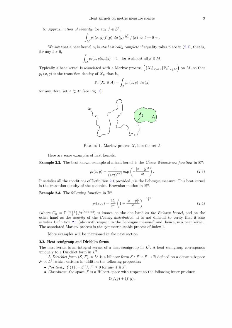
Typically a heat kernel is associated with a Markov process({Xt}t≥0 , {Px}x∈M
)on M , so that
pt (x, y) is the transition density of Xt, that is,
Px (Xt ∈ A) =∫
A
pt (x, y) dμ (y)
for any Borel set A ⊂ M (see Fig. 1).
Xt
x
A
Figure 1. Markov process Xt hits the set A
Here are some examples of heat kernels.
Example 2.2. The best known example of a heat kernel is the Gauss-Weierstrass function in Rn:
pt(x, y) =1
(4πt)n/2exp
(
−|x − y|2
4t
)
. (2.3)
It satisfies all the conditions of Definition 2.1 provided μ is the Lebesgue measure. This heat kernelis the transition density of the canonical Brownian motion in Rn.
Example 2.3. The following function in Rn
pt(x, y) =Cn
tn
(
1 +|x − y|2
t2
)−n+12
(2.4)
(where Cn = Γ(
n+12
)/π(n+1)/2) is known on the one hand as the Poisson kernel, and on the
other hand as the density of the Cauchy distribution. It is not difficult to verify that it alsosatisfies Definition 2.1 (also with respect to the Lebesgue measure) and, hence, is a heat kernel.The associated Markov process is the symmetric stable process of index 1.
More examples will be mentioned in the next section.
2.2. Heat semigroup and Dirichlet forms
The heat kernel is an integral kernel of a heat semigroup in L2. A heat semigroup correspondsuniquely to a Dirichlet form in L2.
A Dirichlet form (E ,F) in L2 is a bilinear form E : F × F → R defined on a dense subspaceF of L2, which satisfies in addition the following properties:
• Positivity : E (f) := E (f, f) ≥ 0 for any f ∈ F .• Closedness : the space F is a Hilbert space with respect to the following inner product:
E(f, g) + (f, g) .
4 Grigor’yan, Hu and Lau
• The Markov property : if f ∈ F then the function
g := min {1, max{f, 0})}
also belongs to F and E (g) ≤ E (f). Here we have used the shorthand E (f) := E (f, f).
Any Dirichlet form has the generator L, which is a non-positive definite self-adjoint operatoron L2 with domain D ⊂ F such that
E (f, g) = (−Lf, g)
for all f ∈ D and g ∈ F . The generator determines the heat semigroup {Pt}t≥0 defined by Pt = etL.The heat semigroup satisfies the following properties:
• {Pt}t≥0 is contractive in L2, that is ‖Ptf‖2 ≤ ‖f‖2 for all f ∈ L2 and t > 0.• {Pt}t≥0 is strongly continuous, that is, for every f ∈ L2,
PtfL2
−→ f as t → 0 + .
• {Pt}t≥0 is symmetric, that is,
(Ptf, g) = (f, Ptg) for all f, g ∈ L2.
• {Pt}t≥0 is Markovian, that is, for any t > 0,
if f ≥ 0 then Ptf ≥ 0, and if f ≤ 1 then Ptf ≤ 1.
Here and below the inequalities between L2-functions are understood μ-almost everywhere inM .
The form (E ,F) can be recovered from the heat semigroup as follows. For any t > 0, definea quadratic form Et on L2 as follows
Et (f) :=1t
(f − Ptf, f) . (2.5)
It is easy to show that Et (f) is non-negative and is increasing as t is decreasing. In particular, ithas the limit as t → 0. It turns out that the limit is finite if and only if f ∈ F , and, moreover,
limt→0+
Et (f) = E (f)
(cf. [9]). Extend Et to a bilinear form as follows
Et(f, g) :=1t
(f − Ptf, g) .
Then, for all f, g ∈ F ,lim
t→0+Et (f, g) = E (f, g) .
The Markovian property of the heat semigroup implies that the operator Pt preserves theinequalities between functions, which allows to use monotone limits to extend Pt from L2 to L∞
and, in fact, to any Lq, 1 ≤ q ≤ ∞. Moreover, the extended operator Pt is a contraction on anyLq (cf. [15, p.33]).
Recall some more terminology from the theory of the Dirichlet form (cf. [15]). The form(E ,F) is called conservative if Pt1 = 1 for every t > 0. The form (E ,F) is called local if E(f, g) = 0for any couple f, g ∈ F with disjoint compact supports. The form (E ,F) is called strongly localif E(f, g) = 0 for any couple f, g ∈ F with compact supports, such that f ≡ const in an openneighborhood of supp g.
The form (E ,F) is called regular if F ∩ C0 (M) is dense both in F and in C0 (M), whereC0(M) is the space of all continuous functions with compact support in M , endowed with thesup-norm. For a non-empty open Ω ⊂ M , let F(Ω) be the closure of F ∩ C0(Ω) in the norm of F .It is known that if (E ,F) is regular, then (E ,F(Ω)) is also a regular Dirichlet form in L2(Ω, μ).
Assume that the heat semigroup {Pt} of a Dirichlet form (E ,F) in L2 admits an integralkernel pt, that is, for all t > 0 and x ∈ M , the function pt (x, ∙) belongs to L2, and the followingidentity holds:
Ptf (x) =∫
M
pt (x, y) f (y) dμ (y) , (2.6)
Heat kernels on metric measure spaces 5
for all f ∈ L2 and μ-a.a. x ∈ M . Then the function pt is indeed a heat kernel, as we will showbelow. For this reason, we also call pt the heat kernel of the Dirichlet form (E ,F) or of the heatsemigroup {Pt}.
Observe that if the heat kernel pt of (E ,F) exists, then by (2.5) and (2.6),
Et(f) =12t
∫
M
∫
M
(f(y) − f(x))2 pt(x, y)dμ(y)dμ(x) (2.7)
+1t
∫
M
(1 − Pt1(x)) f(x)2 dμ(x) (2.8)
for any t > 0 and f ∈ L2.
Proposition 2.4. ([21]) If pt is the integral kernel of the heat semigroup {Pt}, then pt is a heatkernel.
Proof. We will verify that pt satisfies all the conditions in Definition 2.1. Let t > 0 be fixed untilstated otherwise.
(1) Setting pt,x = pt(x, ∙), we see from (2.6) that, for any f ∈ L2,
Ptf(x) = (pt,x, f) for μ-almost all x ∈ M ,
whence it follows that the function x 7→ (pt,x, f) is μ-measurable in x. Let {ϕk}∞k=1 be an orthonor-
mal basis of L2. Using the identity
pt (x, y) = pt,x (y) =∞∑
k=1
(pt,x, ϕk) ϕk (y) ,
we conclude that pt (x, y) is jointly measurable in x, y ∈ M , because so are the functions (pt,x, ϕk) ϕk (y).(2) By the Markovian property of Pt, for any non-negative function f ∈ L2, there is a null
set Nf ⊂ M such thatPtf (x) ≥ 0 for all x ∈ M \ Nf .
Let S be a countable family of non-negative functions, which is dense in the cone of all non-negativefunctions in L2, and set
N =⋃
f∈S
Nf
so that N is a null set. Then Ptf (x) ≥ 0 for all x ∈ M \ N and for all f ∈ S. If f is anyother non-negative function in L2, then f is an L2-limit of a sequence {fk} ⊂ S, whence, for anyx ∈ M \ N ,
(pt,x, f) = limk→∞
(pt,x, fk) = limk→∞
Ptfk (x) ≥ 0.
Therefore, for any x ∈ M \ N , we have that pt,x ≥ 0 μ-a.e. in M , which proves that pt (x, y) ≥ 0for μ-a.a. x, y ∈ M .
Let K ⊂ M be compact. Then the indicator function 1K belongs to L2 and is bounded by 1,whence ∫
K
pt (x, y) dμ (y) = Pt1K (x) ≤ 1
for μ-a.a. x ∈ M . Choosing an increasing sequence of compact sets {Kn}∞n=1 that exhausts M , we
obtain that ∫
M
pt (x, y) dμ (y) = limn→∞
∫
Kn
pt (x, y) dμ ≤ 1
for μ-a.a. x ∈ M .Consequently, for any compact set K ⊂ M , we obtain by Fubini’s theorem
∫
K×M
pt (x, y) dμ(y)dμ(x) =∫
K
(∫
M
pt (x, y) dμ (y)
)
dμ (x)
≤∫
K
dμ (x) = μ (K) < ∞,
which implies that pt (x, y) ∈ L1loc (M × M).

6 Grigor’yan, Hu and Lau
(3) For all f, g ∈ L2, we have, again by Fubini’s theorem,
(Ptf, g) =∫
M×M
pt (x, y) f (y) g (x) dμ(y)dμ (x) . (2.9)
On the other hand, by the symmetry of Pt,
(Ptf, g) = (f, Ptg) =∫
M
Ptg (y) f (y) dμ (y)
=∫
M×M
pt (y, x) f (y) g (x) dμ(y)dμ(x). (2.10)
Comparing (2.9) and (2.10), we obtain pt (x, y) = pt (y, x) for μ-almost all x, y ∈ M .(4) Using the semigroup identity Pt+s = Pt (Ps) and Fubini’s theorem, we obtain that, for
any f ∈ L2 and for μ-a.a. x ∈ M ,
Pt+sf (x) = Pt (Psf) (x)
=∫
M
pt (x, z)
(∫
M
ps (z, y) f (y) dμ (y)
)
dμ (z)
=∫
M
(∫
M
pt(x, z)ps(z, y)dμ(z)
)
f (y) dμ (y) ,
whence, for any g ∈ L2,
(Pt+sf, g) =∫
M×M
(∫
M
pt(x, z)ps(z, y)dμ(z)
)
f (y) g (x) dμ(y)dμ(x).
Comparing with
(Pt+sf, g) =∫
M×M
pt+s (x, y) f (y) g (x) dμ(y)dμ (x) ,
we obtain (2.2).
(5) Finally, the approximation of identity property follows immediately from (2.6) and PtfL2
→f as t → 0. �
Corollary 2.5. If pt and qt are two integral kernels of a heat semigroup {Pt}, then, for any t > 0,
pt (x, y) = qt (x, y) for μ-a.a. x, y ∈ M. (2.11)
Proof. Similarly to (2.9), we have
(Ptf, g) =∫
M×M
qt (x, y) f (y) g (x) dμ(y)dμ (x) .
Comparing with (2.9), we obtain (2.11). �
Remark 2.6. Of course, not every heat semigroup possesses a heat kernel. The existence for theheat kernel and results related to these on-diagonal upper bounds can be found in [4, Theorem2.1], [2, Propositions 4.13, 4.14], [8], [9], [11], [13], [14, Lemma 2.1.2], [17], [21], [23], [31], [40], [41],[42], [43].
2.3. Examples
Example 2.7. Let M be a connected Riemannian manifold, d be the geodesic distance, and μ bethe Riemannian measure. The Laplace-Beltrami operator Δ on M can be made into a self-adjointoperator in L2 (M,μ) by appropriately defining its domain. Then Δ generates the heat semigroupPt = etΔ, which is associated with the local Dirichlet form (E ,F) where
E (f) =∫
M
|∇f |2 dμ, F = W 1,20 (M) .
The corresponding Markov process is a Brownian motion on M .It is known that this {Pt} always has a smooth integral kernel pt (x, y), which is called the
heat kernel of M . Although the explicit expression of pt(x, y) can not be given in general, thereare many important classes of manifolds where pt (x, y) admits certain upper and/or lower bounds.
Heat kernels on metric measure spaces 7
For example, as it was proved in [32], if M is geodesically complete and its Ricci curvature isnon-negative, then
pt(x, y) �1
V(x,
√t) exp
(
−cd(x, y)2
t
)
, x, y ∈ M, t > 0, (2.12)
where V (x, r) = μ (B(x, r)) is the volume of the geodesic ball
B(x, r) = {y ∈ M : d(y, x) < r}.
Example 2.8. If Δ is a self-adjoint Laplace operator as above then the operator L = − (−Δ)β/2
(where 0 < β < 2) generates on M a Markov process with jumps. In particular, if M = Rn thenthis is the symmetric stable process of index β, and the corresponding heat kernel admits thefollowing estimate
pt (x, y) �1
tn/β
(
1 +|x − y|β
t
)−n+ββ
.
A particular case β = 1 was already mentioned in Example 2.3.
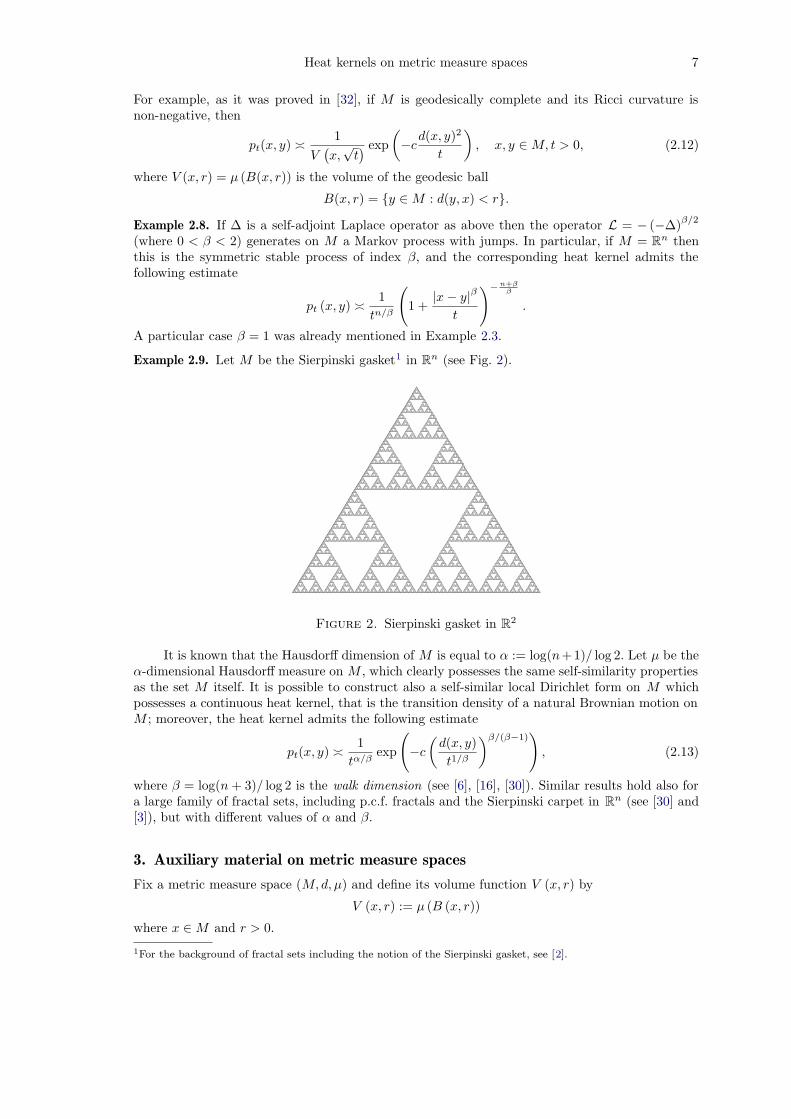
Example 2.9. Let M be the Sierpinski gasket1 in Rn (see Fig. 2).
Figure 2. Sierpinski gasket in R2
It is known that the Hausdorff dimension of M is equal to α := log(n+1)/ log 2. Let μ be theα-dimensional Hausdorff measure on M , which clearly possesses the same self-similarity propertiesas the set M itself. It is possible to construct also a self-similar local Dirichlet form on M whichpossesses a continuous heat kernel, that is the transition density of a natural Brownian motion onM ; moreover, the heat kernel admits the following estimate
pt(x, y) �1
tα/βexp
(
−c
(d(x, y)t1/β
)β/(β−1))
, (2.13)
where β = log(n + 3)/ log 2 is the walk dimension (see [6], [16], [30]). Similar results hold also fora large family of fractal sets, including p.c.f. fractals and the Sierpinski carpet in Rn (see [30] and[3]), but with different values of α and β.
3. Auxiliary material on metric measure spaces
Fix a metric measure space (M,d, μ) and define its volume function V (x, r) by
V (x, r) := μ (B (x, r))
where x ∈ M and r > 0.
1For the background of fractal sets including the notion of the Sierpinski gasket, see [2].

8 Grigor’yan, Hu and Lau
3.1. Besov spaces
Here we introduce function spaces W β/2,p on M . Choose parameters 1 ≤ p < ∞, β > 0 and definethe functional Eβ,p (u) for all functions u ∈ Lp as follows:
Eβ,p(u) = sup0<r≤1
r−pβ/2
∫
M
[1
V (x, r)
∫
B(x,r)
|u(y) − u(x)|p dμ(y)
]
dμ(x). (3.1)
For simplicity, if p = 2, denote it by
Eβ(u) := Eβ,2(u).
The Besov space W β/2,p is defined by
W β/2,p := {u ∈ Lp : Eβ,p(u) < ∞} (3.2)
with the norm‖u‖W β/2,p := ‖u‖p + Eβ,p(u)1/p.
For Ahlfors regular2 measures μ, the Besov space W β/2,p was introduced in [28, 34, 22]although using different notation.
It is not difficult to verify that for any 1 ≤ p < ∞ and β > 0, the space W β/2,p is a Banachspace. Note that the space W β/2,p decreases as β increases; it may happen that this space becomestrivial for large enough β. For example, W β/2,2 (Rn) = {0} for β > 2.
Define the critical Besov exponent β∗ by
β∗ := sup{
β > 0 : W β/2,2 is dense in L2 (M,μ)}
. (3.3)
Lemma 3.1. We have β∗ ≥ 2.
Proof. It suffices to show that W 1,2 is dense in L2 = L2 (M,μ). Let u be a Lipschitz function witha bounded support A and let Ar be the closed r-neighborhood of A. If L is the Lipschitz constantof u, then
E2 (u) = sup0<r≤1
r−2
∫
Ar
1V (x, r)
∫
B(x,r)
|u(y) − u(x)|2 dμ(y)dμ(x)
≤ sup0<r≤1
r−2
∫
Ar
L2r2dμ(x)
≤ L2μ (A1) .
It follows that E2(u) < ∞ and hence u ∈ W 1,2. We are left to show that the class Lip of allLipschitz functions with bounded supports is dense in L2. Indeed, let now A be any boundedclosed subset of M . For any positive integer n, consider the function on M
fn (x) = (1 − nd (x,A))+ ,
which is Lipschitz and is supported in A1/n. Clearly, fn → 1A in L2 as n → ∞, whence it followsthat 1A ∈ Lip, where the bar means the closure in L2. Since the linear combinations of the indicatorfunctions of bounded closed sets form a dense subset in L2, it follows that Lip = L2, which was tobe proved. �
3.2. Doubling condition and reverse doubling condition
The measure μ on M is said to be doubling if there is a constant CD ≥ 1 such that
V (x, 2r) ≤ CDV (x, r) (3.4)
for all x ∈ M and r > 0.
Proposition 3.2. If (3.4) holds on M , then there exists α > 0 depending only on the doublingconstant CD such that
V (x,R)V (y, r)
≤ CD
(d(x, y) + R
r
)α
for all x, y ∈ M and 0 < r ≤ R. (VD)
2A measure μ on a metric space (M, d) is said to be Ahlfors-regular if there exist α, c > 0 such that V (x, r) � rα
for all balls B(x, r) in M with r ∈ (0, 1).

Heat kernels on metric measure spaces 9
Hence, the inequality of Proposition 3.2 can be used as an alternative definition of the doublingproperty of μ and will be referred to as (V D) (volume doubling). The advantage of this definitionis that it introduces a parameter α that will frequently be used.
Proof. If x = y, then R ≤ 2nr where
n =
[
log2
R
r
]
≤ log2
R
r+ 1,
whence, it follows from (3.4) that
V (x,R)V (x, r)
≤V (x, 2nr)V (x, r)
≤ (CD)n ≤ (CD)log2Rr +1 = CD
(R
r
)log2 CD
. (3.5)
If x 6= y, then B (x,R) ⊂ B (y,R + r0) where r0 = d (x, y). By (3.5),
V (x,R)V (y, r)
≤V (y,R + r0)
V (y, r)≤ CD
(R + r0
r
)log2 CD
,
which finishes the proof. �
The measure μ satisfies a reverse volume doubling condition if there exist positive constantsα′ and c such that
V (x,R)V (x, r)
≥ c
(R
r
)α′
for all x ∈ M and 0 < r ≤ R. (RVD)
Proposition 3.3. If (M,d) is connected and μ satisfies (3.4), then there exist positive constants α′
and c such that (RVD) holds, provided B (x,R)c is non-empty.
Proof. The condition B (x,R)c 6= ∅ implies that
B (x, ρ′) \ B (x, ρ) 6= ∅ (3.6)
for all 0 < ρ < R and ρ′ > ρ. Indeed, otherwise M splits into disjoint union of two open sets:B (x, ρ) and B (x, ρ)
c. Since M is connected, the set B (x, ρ)
cmust be empty, which contradicts
the non-emptiness of B (x,R)c.If 0 < ρ ≤ R/2, then we have by (3.6)
B
(
x,53ρ
)
\ B
(
x,43ρ
)
6= ∅.
Let y be a point in this annulus. It follows from (VD) that
V (x, ρ) ≤ CV (y, ρ/3)
for some constant C > 0, whence
V (x, 2ρ) ≥ V (x, ρ) + V (y, ρ/3) ≥ (1 + ε) V (x, ρ) , (3.7)
where ε = C−1.For any 0 < r ≤ R, we have that 2nr ≤ R where
n :=
[
log2
R
r
]
≥ log2
R
r− 1.
For any 0 ≤ k ≤ n − 1, we have 2kr ≤ R/2, and whence by (3.7),
V(x, 2k+1r
)≥ (1 + ε) V (x, 2kr).
Iterating this inequality, we obtain
V (x,R)V (x, r)
≥V (x, 2nr)V (x, r)
≥ (1 + ε)n
≥ (1 + ε)log2Rr −1 = (1 + ε)−1
(R
r
)log2(1+ε)
,
thus proving (RVD). �

10 Grigor’yan, Hu and Lau
Remark 3.4. As one can see from the argument after (3.7), the measure μ is reverse doublingwhenever the following inequality holds
V (x,Cr) ≥ (1 + ε) V (x, r) (3.8)
for some C > 1, ε > 0 and all x ∈ M , r > 0.
Corollary 3.5. Assume that (M,d) is connected and μ satisfies (VD). Then
μ (M) = ∞ ⇔ diam(M) = ∞ ⇔ (RVD).
Proof. If μ (M) = ∞, then diam(M) = ∞; indeed, otherwise M would be a ball of a finite radiusand its measure would be finite by (VD). If diam(M) = ∞, then Bc (x,R) 6= ∅ for any ball B (x,R),and (RVD) holds by Proposition 3.3. Finally, (RVD) implies μ (M) = ∞ by letting R → ∞ in(RVD). �
4. Consequences of heat kernel estimates
We give here some consequences of the heat kernel estimates
1
V(x, t1/β
)Φ1
(d(x, y)t1/β
)
≤ pt (x, y) ≤1
V(x, t1/β
)Φ2
(d(x, y)t1/β
)
,
for all t > 0 and μ-almost all x, y ∈ M . Functions Φ1 (s) and Φ2 (s) are always assumed to benon-negative and monotone decreasing on [0, +∞), the constant β is positive.
We prove that
• The lower estimate of the heat kernel implies that– the measure μ is doubling;– the space F is embedded in W β/2,2;– the lower tail function Φ1 (s) is controlled from above by a negative power of s.
• The upper estimate of the heat kernel implies that– the space W β/2,2 is embedded in F ;– if the Dirichlet form is non-local then the upper tail function Φ2 (s) is controlled from
below by a negative power of s (for large s).
4.1. Consequences of lower bound
Let pt be a heat kernel on a metric measure space (M,d, μ). Consider the lower estimate of pt ofthe form:
pt (x, y) ≥1
V(x, t1/β
)Φ1
(d(x, y)t1/β
)
(4.1)
for all t > 0 and μ-almost all x, y ∈ M .
Lemma 4.1. Assume that the heat kernel pt satisfies the lower bound (4.1). If Φ1(s0) > 0 for somes0 > 1, then μ is doubling.
Proof. Fix r, t > 0 and consider the following integral∫
B(x,r)
pt(x, y)dμ(y) :=∫
M
pt(x, y)1B(x,r)(y) dμ(y).
The right-hand side is understood as follows: the function
F (x, y) := pt(x, y)1B(x,r)(y)
is measurable jointly in x, y so that, by Fubini’s theorem, the integral∫
M
pt(x, y)1B(x,r)(y) dμ(y)
is well-defined for μ-almost all x ∈ M and is a measurable function of x. Choose any pointwiseversion of pt(x, y) as a function of x, y. By Fubini’s theorem, there is a subset M0 ∈ M of full
Heat kernels on metric measure spaces 11
measure such that, for any x ∈ M0, the function pt(x, y) is measurable in y and the inequalities(4.1) and (2.1) hold for μ-a.a. y ∈ M . It follows that, for all x ∈ M0,
∫
B(x,r)
pt(x, y)dμ(y) ≤ 1 (4.2)
whence1
V (x, r)≥ einf
y∈B(x,r)pt(x, y).
On the other hand, we have by (4.1)
einfy∈B(x,r)
pt(x, y) ≥1
V (x, t1/β)Φ1
( r
t1/β
),
which together with the previous estimate gives
V (x, r)
V(x, t1/β
) ≤1
Φ1
(r/t1/β
) .
Setting here t = (r/s0)β we obtain
V (x, r)V (x, r/s0)
≤1
Φ1 (s0). (4.3)
Since s0 > 1 and Φ1 (s0) > 0, (4.3) implies that measure μ is doubling. �
Lemma 4.2. Assume that the heat kernel pt satisfies the lower bound (4.1) with Φ1(s0) > 0 forsome s0 ≥ 1. Then, there is a constant c > 0 such that for all u ∈ L2 (M),
E(u) ≥ cEβ(u). (4.4)
Consequently, the space F embeds into W β/2,2.
Proof. Let t, r > 0. It follows from (2.7) and the lower bound (4.1) that
E(u) ≥ Et(u) ≥12t
∫
M
∫
B(x,r)
(u(y) − u(x))2 pt(x, y)dμ(y)dμ(x)
≥12t
Φ1
( r
t1/β
)∫
M
(1
V (x, t1/β)
∫
B(x,r)
(u(y) − u(x))2 dμ(y)
)
dμ(x),
where we have used the monotonicity of Φ1. Choosing t = (r/s0)β and noticing that V (x, r/s0) ≤
V (x, r) by s0 ≥ 1, we obtain
E(u) ≥sβ0
2rβΦ1 (s0)
∫
M
(1
V (x, r)
∫
B(x,r)
(u(y) − u(x))2 dμ(y)
)
dμ(x),
whence, by taking supremum in r,
E(u) ≥12sβ0Φ1(s0)Eβ(u),
thus proving (4.4). �
Finally, we give another consequences of the lower bound (4.1) of the heat kernel.
Lemma 4.3. Assume that the heat kernel pt satisfies the lower bound (4.1). If μ satisfies the reversedoubling property (RVD), then there is c > 0 such that
Φ1(s) ≤ c(1 + s)−(α′+β) for all s > 0, (4.5)
where α′ is the same as in (RVD).

12 Grigor’yan, Hu and Lau
{ }
{ }
Figure 3. Sets A and B
Proof. Following [24], let u ∈ L2 be a non-constant function. Choose a ball B(x0, R) where u isnon-constant and let a > b be two real values such that the sets
A = {x ∈ B(x0, R) : u(x) ≥ a} and B = {x ∈ B(x0, R) : u(x) ≤ b}
both have positive measure (see Fig. 3).It follows from (2.7) that
E(u) ≥12t
∫
M
∫
M
(u(y) − u(x))2 pt(x, y)dμ(y)dμ(x)
≥12t
∫
A
∫
B
(a − b)21
V (x, t1/β)Φ1
(2R
t1/β
)
dμ(y)dμ(x)
=(a − b)2
2tΦ1
(2R
t1/β
)
μ(B)∫
A
1V (x, t1/β)
dμ(x).
For x ∈ A, we have that B(x,R) ⊂ B(x0, 3R), and hence, for small enough t > 0,
1V (x, t1/β)
=1
V (x,R)∙
V (x,R)V (x, t1/β)
≥1
V (x0, 3R)∙ c
(R
t1/β
)α′
,
where we have used the reverse doubling property (RVD). Therefore, for small t > 0,
E(u) ≥c′(a − b)2
V (x0, 3R)Rβμ(A)μ(B)
(2R
t1/β
)α′+β
Φ1
(2R
t1/β
)
.
If (4.5) fails, then there exists a sequence {sk} with sk → ∞ as k → ∞ such that
sα′+βk Φ1(sk) → ∞ as k → ∞.
Choose tk such that sk = 2R/t1/βk . Then
(2R
t1/βk
)α′+β
Φ1
(2R
t1/βk
)
= sα′+βk Φ1(sk) → ∞
as k → ∞, and hence E(u) = ∞. Hence, we see that F consists only of constants. Since F is densein L2, it follows that L2 also consists of constants only. Hence, there is a point x ∈ M with apositive mass, that is, μ ({x}) > 0. Then (2.1) implies that, for all t > 0,
pt(x, x) ≤1
μ({x}). (4.6)
However, by (RVD), we have V (x, r) → 0 as r → 0, which together with (4.1) implies thatpt(x, x) → ∞ as t → 0, thus contradicting (4.6). �
Heat kernels on metric measure spaces 13
Remark 4.4. The last argument in the above proof can be stated as follows. If (RVD) is satisfiedand (4.1) holds with a function Φ1 such that Φ1 (0) > 0, then μ ({x}) = 0 for all x ∈ M . Thissimple observation will also be used below.
4.2. Consequences of upper bound
Consider the upper estimate of pt of the form:
pt (x, y) ≤1
V(x, t1/β
)Φ2
(d(x, y)t1/β
)
(4.7)
for all t > 0 and μ-almost all x, y ∈ M .
Lemma 4.5. Assume that μ satisfies both (VD) and (RVD), and that the heat kernel pt is stochas-tically complete and satisfies the upper bound (4.7) with
∫ ∞
0
sα+β−1Φ2(s)ds < ∞, (4.8)
where α is the same as in (VD). Then, there is a constant c > 0 such that for all u ∈ L2 (M),
E(u) ≤ CEβ(u). (4.9)
Consequently, the space W β/2,2 embeds into F .
Proof. Fix t ∈ (0, 1) and let n be the smallest negative integer such that 2n+1 ≥ t1/β . Since pt isstochastically complete, we have that for any t > 0,
Et (u) =12t
∫
M
∫
M
(u(x) − u(y))2pt(x, y)dμ(y)dμ(x) = A0(t) + A1(t) + A2 (t) (4.10)
where
A0(t) : =12t
∫
M
∫
B(x,1)c
(u(x) − u(y))2pt(x, y)dμ(y)dμ(x), (4.11)
A1(t) : =12t
∫
M
∫
B(x,1)\B(x,2n)
(u(x) − u(y))2pt(x, y)dμ(y)dμ(x), (4.12)
A2(t) : =12t
∫
M
∫
B(x,2n)
(u(x) − u(y))2pt(x, y)dμ(y)dμ(x). (4.13)
Observing that by (VD)
V (x, 2k+1)V (x, t1/β)
≤ C
(2k+1
t1/β
)α
for all k ≥ n, (4.14)
and using (4.7), we obtain
∫
B(x,1)c
pt(x, y)dμ(y) ≤∞∑
k=0
∫
B(x,2k+1)\B(x,2k)
1V (x, t1/β)
Φ2
(2k
t1/β
)
dμ(y)
≤ C
∞∑
k=0
V (x, 2k+1)V (x, t1/β)
Φ2
(2k
t1/β
)
≤ C ′∞∑
k=0
(2k
t1/β
)α
Φ2
(2k
t1/β
)
≤ C ′∫ ∞
12 t−1/β
sα−1Φ2(s)ds (4.15)
≤ ct
∫ ∞
12 t−1/β
sα+β−1Φ2(s)ds. (4.16)
14 Grigor’yan, Hu and Lau
Applying the elementary inequality (a − b)2 ≤ 2(a2 + b2), we obtain from (4.11)
A0(t) ≤1t
∫
M
∫
B(x,1)c
(u(x)2 + u(y)2)pt(x, y)dμ(y)dμ(x)
=2t
∫
M
u(x)2(∫
B(x,1)c
pt(x, y)dμ(y)
)
dμ(x)
≤ 2c‖u‖22
∫ ∞
12 t−1/β
sα+β−1Φ2(s)ds
= o(1)‖u‖22 as t → 0, (4.17)
where we have used (4.8). It follows that
limt→0+
A0(t) = 0. (4.18)
By (4.7) and (4.14), we obtain that, for 0 > k ≥ n,
∫
B(x,2k+1)\B(x,2k)
(u(x) − u(y))2pt(x, y)dμ(y)
≤1
V (x, t1/β)Φ2
(2k
t1/β
)∫
B(x,2k+1)\B(x,2k)
(u(x) − u(y))2dμ(y)
≤ c
(2k+1
t1/β
)α
Φ2
(2k
t1/β
)1
V (x, 2k+1)
∫
B(x,2k+1)
(u(x) − u(y))2dμ(y).
By the definition (3.1) of Eβ , for all k < 0,
∫
M
1V (x, 2k+1)
∫
B(x,2k+1)
(u(x) − u(y))2dμ(y)dμ (x) ≤(2k+1
)βEβ (u) . (4.19)
Therefore, we obtain
A1 (t) =12t
∑
n≤k<0
∫
M
∫
B(x,2k+1)\B(x,2k)
(u(x) − u(y))2pt(x, y)dμ(y)dμ(x)
≤12t
∑
n≤k<0
c
(2k+1
t1/β
)α
Φ2
(2k
t1/β
)
×∫
M
1V (x, 2k+1)
∫
B(x,2k+1)
(u(x) − u(y))2dμ(y)dμ (x) (4.20)
≤ c∑
n≤k<0
(2k+1
t1/β
)α+β
Φ2
(2k
t1/β
)
Eβ(u)
≤ cEβ(u)∫ ∞
0
sα+β−1Φ2(s)ds, (4.21)
where the latter integral converges due to (4.8).
For k < n, we have 2k+1 < t1/β whence by (RVD)
V (x, 2k+1)V (x, t1/β)
≤ c
(2k+1
t1/β
)α′
. (4.22)

Heat kernels on metric measure spaces 15
Similarly to the estimate of A1, we obtain
A2 (t) =12t
∑
k<n
∫
M
∫
B(x,2k+1)\B(x,2k)
(u(x) − u(y))2pt(x, y)dμ(y)dμ(x)
≤ c∑
k<n
(2k+1
t1/β
)α′+β
Φ2
(2k
t1/β
)
Eβ(u)
≤ cEβ(u)∫ 2
0
sα′+β−1Φ2(s)ds, (4.23)
where the latter integral converges at 0 due to α′ +β > 0. It follows from (4.10), (4.18), (4.21) and(4.23) that
E(u) = limt→0+
Et (u) = limt→0+
(A0 (t) + A1 (t) + A2 (t)) ≤ CEβ(u),
which finishes the proof. �
Lemma 4.6. Assume that μ satisfies (VD) and that the heat kernel pt satisfies the upper bound(4.7). Then, either (E ,F) is local, or there is c > 0 such that
Φ2(s) ≥ c(1 + s)−(α+β) for all s > 0. (4.24)
Proof. Let u, v ∈ F be functions with disjoint compact supports A = supp u and B = supp v (seeFig. 4).
A BR
Figure 4. Functions u and v
Noticing that (u, v) = 0, we obtain, for any t > 0,
Et(u, v) =1t
(u, v − Ptv)
= −1t
(u, Ptv)
= −1t
∫
A
u(x)
(∫
B
v(y)pt(x, y)dμ(y)
)
dμ(x).
Setting R = d(A,B) > 0 and using (4.7), we obtain
|Et(u, v)| ≤1tΦ2
(R
t1/β
)
‖v‖1
∫
A
|u(x)|V (x, t1/β)
dμ(x). (4.25)
Choose any fixed point x0 ∈ A and let diam(A) = r. Then, using (VD), we see that, for all x ∈ Aand small t > 0,
1V (x, t1/β)
=1
V (x0, r)V (x0, r)
V (x, t1/β)
≤c
V (x0, r)
(d(x0, x) + r
t1/β
)α
≤c
V (x0, r)
(2r
t1/β
)α
.
Therefore, by (4.25),
|Et(u, v)| ≤1tΦ2
(R
t1/β
)
‖v‖1c
V (x0, r)
(2r
t1/β
)α
‖u‖1
=c(2r)α
V (x0, r)Rα+β‖u‖1‖v‖1
(R
t1/β
)α+β
Φ2
(R
t1/β
)
.

16 Grigor’yan, Hu and Lau
If (4.24) fails, then there exists a sequence {sk} such that sk → ∞ as k → ∞, and
sα+βk Φ2(sk) → 0.
Letting tk > 0 such that sk = R/t1/βk , we obtain that
|Etk(u, v)| → 0 as k → ∞,
showing that E(u, v) = 0. Hence, the (E ,F) is local, which was to be proved. �
4.3. Walk dimension
Here we obtain certain consequence of a two-sided estimate
1
V(x, t1/β
)Φ1
(d(x, y)t1/β
)
≤ pt (x, y) ≤1
V(x, t1/β
)Φ2
(d(x, y)t1/β
)
. (4.26)
The parameter β from (4.26) is called the walk dimension of the associated Markov process.
Theorem 4.7. Assume that μ satisfies both (VD) and (RVD). Let the heat kernel pt (x, y) be stochas-tically complete and satisfy (4.26) where Φ1 (s0) > 0 for some s0 ≥ 1 and
∫ ∞
0
sα+β+εΦ2(s)ds
s< ∞ (4.27)
for some ε > 0. Then β = β∗ where β∗ is the critical Besov exponent defined in (3.3).
Remark 4.8. Assuming in addition that Φ1 (s0) > 0 for some s0 > 1 allows to drop (VD) fromthe hypothesis, thanks to Lemma 4.1. If one assumes on top of that, that the metric space (M,d)is connected and has infinite diameter then (RVD) follows from (VD) by Corollary 3.5. Hence, inthis case (RVD) can be dropped from the assumptions as well.
Proof. By Lemma 4.2, we have the inclusion F ⊂ W β/2,2. Since F is always dense in L2, weconclude that W β/2,2 is dense in L2, whence β∗ ≥ β.
To prove the opposite inequality, it suffices to verify that, for any β′ > β, the space W β′/2,2 isnot dense in L2. We can assume that β′ − β is sufficiently small so that the condition (4.27) holdswith ε = β′ − β.
Let us show that u ∈ W β′/2,2 implies E (u) = 0. We use again the decomposition
Et (u) = A0(t) + A1(t) + A2 (t)
where Ai(t) are defined in (4.11)–(4.13). As in the proof of Lemma 4.5, we have
limt→0
A0 (t) = 0.
Let us estimate A1(t) similarly to the proof of Lemma 4.5 (and using the same notation), but useEβ′ instead of Eβ . Indeed, using instead of (4.19) the inequality
∫
M
1V (x, 2k+1)
∫
B(x,2k+1)
(u(x) − u(y))2dμ(y)dμ (x) ≤(2k+1
)β′
Eβ′ (u) , (4.28)
we obtain from (4.20) that
A1(t) ≤ ctβ′
β −1∑
n≤k<0
(2k+1
t1/β
)α+β′
Φ2
(2k
t1/β
)
Eβ′(u)
≤ ctβ′
β −1Eβ′(u)∫ ∞
0
sα+β′−1Φ2(s)ds (4.29)
where the integral converges due to (4.27). In the same way, one obtains
A2 (t) ≤ ctβ′
β −1Eβ′(u)∫ 2
0
sα′+β′−1Φ2(s)ds.
Putting together all the estimates, we obtain
Et (u) ≤ A0(t) + Ctβ′
β −1Eβ′(u) → 0 as t → 0,

Heat kernels on metric measure spaces 17
whenceE (u) = lim
t→0Et (u) = 0.
Since Et (u) ≤ E (u), this implies back that Et (u) ≡ 0 for all t > 0.On the other hand, it follows from (2.7) and the lower bound in (4.26) that
Et (u) ≥12t
∫ ∫
{d(x,y)≤s0t1/β}
(u(y) − u(x))2 pt(x, y)dμ(y)dμ(x)
≥Φ1(s0)
2t
∫ ∫
{d(x,y)≤s0t1/β}
(u(x) − u(y))2
V(x, t1/β
) dμ(y)dμ(x),
which yields u(x) = u(y) for μ-almost all x, y such that d(x, y) ≤ s0t1/β . Since t is arbitrary, we
conclude that u is a constant function.Hence, we have shown that the space W β′/2,2 consists of constants. However, it follows from
Remark 4.4 that the constant functions are not dense in L2, which finishes the proof. �
4.4. Consequence of two-sided estimates (non-local case)
Lemmas 4.3 and 4.6 of the previous subsections imply immediately the following.
Theorem 4.9. Assume that the metric measure space (M,d, μ) satisfies (VD) and (RVD). Let {pt}be a heat kernel on M such that, for all t > 0 and almost all x, y ∈ M ,
C ′1
V(x, t1/β
)Φ
(
C1d (x, y)t1/β
)
≤ pt (x, y) ≤C ′
2
V(x, t1/β
)Φ
(
C2d (x, y)t1/β
)
(4.30)
where C1, C′1, C2, C
′2 are positive constants. Then either the associated Dirichlet form E is local or
c1 (1 + s)−(α+β) ≤ Φ(s) ≤ c2 (1 + s)−(α′+β) (4.31)
for all s > 0 and some c1, c2 > 0, where α and α′ are the exponents from (VD) and (RVD),respectively.
5. A maximum principle and its applications
5.1. Weak differentiation
Let H be a Hilbert space over R and I be an interval in R. We say that a function u : I → H isweakly differentiable at t ∈ I if for any ϕ ∈ H, the function (u (∙) , ϕ) is differentiable at t (wherethe outer brackets stand for the inner product in H), that is, the limit
limε→0
(u (t + ε) − u (t)
ε, ϕ
)
exists. In this case it follows from the principle of uniform boundedness that there is w ∈ H suchthat
limε→0
(u (t + ε) − u (t)
ε, ϕ
)
= (w,ϕ)
for all ϕ ∈ H. We refer to the vector w as the weak derivative of the function u at t and writew = u′ (t). Of course, we have the weak convergence
u (t + ε) − u (t)ε
⇀ u′ (t) as ε → 0.
In the next statement, we collect the necessary elementary properties of weak differentiation.
Lemma 5.1. (i) If u is weakly differentiable at t then u is strongly (that is, in the norm of H)continuous at t.
(ii) (The product rule) If functions u : I → H and v : I → H are weakly differentiable at t,then the inner product (u, v) is also differentiable at t and
(u, v)′ = (u′, v) + (u, v′) .
18 Grigor’yan, Hu and Lau
(iii) (The chain rule) Let ( M,μ) be a measure space and set H = L2 ( M,μ). Let u : I →L2 ( M,μ) be weakly differentiable at t ∈ I. Let Φ be a smooth real-valued function on R such that
Φ(0) = 0, supR
|Φ′| < ∞, supR
|Φ′′| < ∞. (5.1)
Then the function Φ(u) : I → L2 ( M,μ) is also weakly differentiable at t and
Φ(u)′ = Φ′ (u) u′.
Proof. To shorten the notation, we write ut for u (t).(i) It suffices to verify that, for any sequence {εk} → 0, we have
‖ut+εk− ut‖ → 0 as k → ∞. (5.2)
The sequenceut+εk
−ut
εkconverges weakly, whence it follows that it is weakly bounded and, hence,
also strongly bounded. The latter clearly implies (5.2).(ii) Let {εk} be as above. We have the identity
(ut+εk, vt+εk
) − (ut, vt)εk
=
(ut+εk
− ut
εk, vt
)
+
(
ut,vt+εk
− vt
εk
)
+
(ut+εk
− ut
εk, vt+εk
− vt
)
.
By the definition of the weak derivative, the first two terms in the right hand side converge to(u′
t, vt) and (ut, v′t) respectively. By part (i), the sequence
ut+εk−ut
εkis bounded in norm, whereas
‖vt+εk− vt‖ → 0 as k → ∞; hence, the third term goes to 0, and we obtain the desired.
(iii) By (5.1) the function Φ admits the estimate |Φ(r)| ≤ C |r| for all r ∈ R, which impliesthat the function Φ (ut) belongs to L2 ( M,μ) for any t ∈ I. By the mean value theorem, for anyr, s ∈ R, there exists ξr,s ∈ (0, 1) such that
Φ (r + s) − Φ(r) = Φ′(r + ξr,s (r − s)
)s.
We have thenΦ (ut+εk
) − Φ(ut)εk
= Φ′ (ut + ξk (ut+εk− ut))
ut+εk− ut
εk,
where we write for simplicity ξk := ξut,ut+εk−ut
. Rewrite this in the form
Φ (ut+εk) − Φ(ut)εk
= Ak + Bk,
where
Ak = (Φ′ (ut + ξk (ut+εk− ut)) − Φ′ (ut))
ut+εk− ut
εk
and
Bk = Φ′ (ut)ut+εk
− ut
εk.
Since‖ (Φ′ (ut + ξk (ut+εk
− ut)) − Φ′ (ut)) ‖L2 ≤ sup |Φ′′| ‖ut+εk− ut‖L2 −→
k→∞0
and the norm∥∥∥
ut+εk−ut
εk
∥∥∥
L2is uniformly bounded, we obtain that ‖Ak‖L1 −→ 0 as k → ∞. Since
‖(Φ′ (ut + ξk (ut+εk− ut)) − Φ′ (ut))‖L∞ ≤ 2 sup |Φ′| < ∞,
we see that the norm ‖Ak‖L2 is uniformly bounded. It follows that Ak → 0 weakly in L2.We are left to verify that Bk → Φ′ (ut) u′
t weakly in L2. Indeed, for any ϕ ∈ L2 ( M,μ), wehave that
(Bk, ϕ) =
(ut+εk
− ut
εk, Φ′ (ut) ϕ
)
→ (u′t, Φ
′ (ut) ϕ) = (Φ′ (ut) u′t, ϕ) ,
where we have used the fact that Φ′ (ut) is bounded and, hence, Φ′ (ut) ϕ ∈ L2 ( M,μ). �
Heat kernels on metric measure spaces 19
5.2. Maximum principle for weak solutions
As before, let (E ,F) be a regular Dirichlet form in L2 (M,μ). Consider a path u : I → F . We saythat u is a weak subsolution of the heat equation in an open set Ω ⊂ M if u is weakly differentiablein the space L2 (Ω) at any t ∈ I and, for any non-negative ϕ ∈ F (Ω),
(u′, ϕ) + E (u, ϕ) ≤ 0. (5.3)
Similarly one defines the notions of weak supersolution and weak solution.A similar definition was introduced in [20] but with the difference that the time derivative
u′ was understood in the sense of the norm convergence in L2 (Ω). Let us refer to the solutionsdefined in [20] as semi-weak solutions. Clearly, any semi-weak solution is also a weak solution.
It is easy to see that, for any f ∈ L2 (M), the function Ptf is a weak solution in (0,∞) × Ωfor any open Ω ⊂ M (cf. [20, Example 4.10]).
Proposition 5.2 (parabolic maximum principle). Let u be a weak subsolution of the heat equationin (0, T )×Ω, where T ∈ (0, +∞] and Ω is an open subset of M . Assume in addition that u satisfiesthe following boundary and initial conditions:
• u+(t, ∙) ∈ F(Ω) for any t ∈ (0, T );
• u+ (t, ∙)L2(Ω)−→ 0 as t → 0.
Then u(t, x) ≤ 0 for any t ∈ (0, T ) and μ-almost all x ∈ Ω.
Remark 5.3. For semi-weak solutions the maximum principle was proved in [20].
Remark 5.4. It was shown in [20, Lemma 4.4] that the condition u+ ∈ F (Ω) is equivalent to thefollowing: u ∈ F and u ≤ v for some v ∈ F(Ω). We will use this result to verify the boundarycondition of the parabolic maximum principle.
Proof. Let Φ be a smooth function on R that satisfies the following conditions for some constantC:
(i) Φ (r) = 0 for all r ≤ 0;(ii) 0 < Φ′ (r) ≤ C for all r > 0.(iii) |Φ′′ (r)| ≤ C for all r > 0.
Then Φ (u) = Φ (u+) ∈ F (Ω) so that we can set ϕ = Φ(u) in (5.3) and obtain
(u′, Φ(u)) + E (u, Φ(u)) ≤ 0.
Since Φ is increasing and Lipschitz, we conclude by [20, Lemma 4.3] that E (u, Φ(u)) ≥ 0, whenceit follows that
(u′, Φ(u)) ≤ 0. (5.4)
Since Φ satisfies the conditions (5.1), we conclude by Lemma 5.1, that the function t 7→ Φ(u) isweakly differentiable in the space L2 (Ω) and
Φ (u)′ = Φ′ (u) u′,
and (u, Φ(u)) is differentiable in t and
(u, Φ(u))′ = (u′, Φ(u)) +(u, Φ(u)′
)
= (u′, Φ(u)) + (u, Φ′ (u) u′)
= (u′, Φ(u)) + (u′, Φ′ (u) u) .
Set Ψ (r) = Φ′ (r) r so that
(u, Φ(u))′ = (u′, Φ(u)) + (u′, Ψ(u)) .
Assume for a moment that function Ψ also satisfies the above properties (i)-(iii). Applying (5.4)to Ψ, we obtain from the previous line
(u, Φ(u))′ ≤ 0,
that is, the function t 7→ (u, Φ(u)) is decreasing in t. By the properties (i)-(ii), we have Φ (r) ≤ Crfor r > 0, which implies
(u, Φ(u)) = (u+, Φ(u+)) ≤ C‖u+‖2 → 0 as t → 0.

20 Grigor’yan, Hu and Lau
Hence, the function t 7→ (u+, Φ(u+)) is non-negative, decreasing and goes to 0 as t → 0, whichimplies that this function is identical 0. It follows that u+ = 0, which was to be proved.
We are left to specify the choice of Φ so that the function Ψ (r) = Φ′ (r) r is also in the class(i)-(iii). Let us construct Φ from its derivative Φ′ that can be chosen to satisfy the following:
• Φ′ (r) = 0 for r ≤ 0;• Φ′ (r) = 1 for r ≥ 1;• Φ′′ (r) > 0 for r ∈ (0, 1).
(see Fig. 5).
0
Φ(r)
r1
Figure 5. Function Φ (r)
Clearly, Φ satisfies (i)-(iii) . It follows from the identity
Ψ′ (r) = Φ′′ (r) r + Φ′ (r)
that Ψ′ (r) is bounded and Ψ′ (r) > 0 for r > 0. Finally, we have
Ψ′′ (r) = Φ′′′ (r) r + 2Φ′′ (r)
whence it follows that Ψ′′ (r) = 0 for large enough r and, hence, Ψ′′ is bounded. We conclude thatΨ satisfies (i)-(iii), which finishes the proof. �
5.3. Some applications of the maximum principle
Recall that if (E ,F) is a regular Dirichlet form in L2 (M,μ) then, for any open set Ω, (E ,F (Ω)) isalso a regular Dirichlet form in L2 (Ω, μ). Denote by PΩ
t the heat semigroup of (E ,F(Ω)).
Lemma 5.5. Assume that (E ,F) is a regular and local Dirichlet form. Let u (t, x) be a weak sub-solution of the heat equation in (0,∞) × U , where U is an open subset of M . Assume further, forany t > 0, u (t, ∙) is bounded in M and is non-negative in U . If
u (t, ∙)L2(U)−→ 0 as t → 0 (5.5)
then the following inequality holds for all t > 0 and almost all x ∈ U :
u (t, x) ≤(1 − PU
t 1U (x))
sup0<s≤t
‖u (s, ∙) ‖L∞(U). (5.6)
Proof. We first assume that U is precompact. Choose an open set W such that W b U. Fix a realT > 0 and set
m := sup0<s≤T
‖u (s, ∙)‖L∞(U) . (5.7)
We show that, for all 0 < t ≤ T and μ-almost all x ∈ W ,
u (t, x) ≤ m(1 − PW
t 1W (x)). (5.8)
Heat kernels on metric measure spaces 21
Let ζ and η be cut-off functions3 of the couples (W,U) and (U,M), respectively. Consider thefunction
w := ζu − m[η − PW
t 1W
]. (5.9)
Then (5.8) will follow if we prove that w ≤ 0 in (0, T ] × W .Claim 1. The w is a weak subsolution of the heat equation in (0,∞) × W .Clearly, PW
t 1W is a weak solution of the heat equation in (0,∞) × W . Let us show that sois ζu. Indeed, the product ζu belongs to F because both ζ and u are in L∞ ∩ F . For any testfunction ψ ∈ F(W ), we have, using ζψ ≡ ψ,
(∂ (ζu)
∂t, ψ
)
=
(
ζ∂
∂tu, ψ
)
=
(∂
∂tu, ψ
)
= −E (u, ψ) = −E (ζu, ψ) + E ((ζ − 1)u, ψ)
= −E (ζu, ψ) ,
where we have used also that (ζ − 1) u = 0 in W and, hence,
E ((ζ − 1)u, ψ) = 0,
by the locality of (E ,F). Thus, ζu is a weak solution in (0,∞) × W .Finally, the function η (x) considered as a function of (t, x), is a weak supersolution of the
heat equation in (0,∞) × W , since for any non-negative ψ ∈ F(W )
E(η, ψ) = limt→0
t−1 (η − Ptη, ψ) = limt→0
t−1 (1 − Ptη, ψ) ≥ 0,
whence it follows that w is a weak subsolution.Claim 2. For every t ∈ (0, T ], we have (w (t, ∙))+ ∈ F(W ).By Remark 5.4, it suffices to prove that in (0, T ] × M
w (t, ∙) ≤ mPWt 1W , (5.10)
because mP Wt 1W ∈ F (W ). In M \ U , inequality (5.10) holds trivially because
ζ = 0 = PWt 1W in M \ U
and, hence, w = −mη ≤ 0. To prove (5.10) in U , observe that η = 1 in U and 0 ≤ u ≤ m in(0, T ] × U , whence
w = ζu − m + mPWt 1W ≤ u − m + mP W
t 1W ≤ mP Wt 1W ,
which was to be proved.Claim 3. The function w satisfies the initial condition
w (t, ∙)L2(W )−→ 0 as t → 0. (5.11)
Noticing that η = 1 in W , we see that
η − PWt 1W = 1W − PW
t 1WL2(W )−→ 0 as t → 0.
Combining with (5.5), we obtain (5.11).By the parabolic maximum principle (cf. Prop. 5.2), we obtain from Claims 1-3 that w ≤ 0
in (0, T ] × W , thus proving (5.8).Finally, let U be an arbitrary open subset of M . Let {Wi}
∞i=1 and {Ui}
∞i=1 be two increasing
sequences of precompact open sets, both of which exhaust U , and such that Wi b Ui for all i. Foreach i, we have by (5.8) with t = T that in Wi
u ≤[1 − PWi
t 1Wi
]sup
0<s≤t‖u (s, ∙)‖L∞(Ui)
. (5.12)
Replacing by the monotonicity in the right hand side Ui by U , and noticing that
PWit 1Wi
a.e.−→ PU
t 1U as i → ∞,
3A cut-off function for the couple (W, U) is a function ζ ∈ F ∩ C0(M) such that 0 ≤ ζ ≤ 1 in M , ζ = 1 on an
open neighborhood of W , and supp ζ ⊂ U . If (E ,F) is a regular Dirichlet form then a cut-off function exists for any
couple (W, U) provided U is open and W is a compact subset of U (cf. [15, p.27]).

22 Grigor’yan, Hu and Lau
we obtain (5.6) by letting i → ∞ in (5.12). �
Corollary 5.6. Assume that (E ,F) is regular and strongly local. Let U ⊂ Ω be two open subsets ofM . Then the following inequality holds for all t > 0 and μ-almost all x ∈ U :
1 − PΩt 1Ω(x) ≤
(1 − PU
t 1U (x))
sup0<s≤t
∥∥1 − PΩ
s 1Ω
∥∥
L∞(U). (5.13)
Proof. Approximating U by precompact open subsets, it suffices to prove the claim in the casewhen U b Ω. Let ϕ be a cut-off function of the couple (U, Ω). Then we can replace the term1 − PΩ
t 1Ω(x) in the both sides of (5.13) by the function
u (t, x) = ϕ (x) − PΩt 1Ω(x).
Clearly, for any t > 0, the function u (t, ∙) is bounded in M , non-negative in U , and satisfiesthe initial condition (5.5). Let us verify that u (t, x) is a weak solution of the heat equation in(0,∞) × U . It suffices to show that the function ϕ (x) as a function of (t, x) is a weak solution in(0,∞)×U . Indeed, since ϕ is constant in a neighborhood of U , the strong locality of (E ,F) yieldsthat E(ϕ,ψ) = 0 for any ψ ∈ F(U), which finishes the proof. �
6. Upper bounds in the local case
6.1. Exponential tail
Following [21], we give an analytical approach of how to obtain the exponential tail of the heatkernel upper bound on the doubling space. This is a modification of the argument of [27]. For analternative approach see [20] (and [25] for the case of infinite graphs).
The following is a key technical lemma.
Lemma 6.1. Let (E ,F) be a regular, strongly local Dirichlet form in L2(M,μ). Let ρ : [0,∞) →[0,∞) be an increasing function. Assume that there exist ε ∈ (0, 1
2 ) and δ > 0 such that, for anyball B ⊂ M of radius r and any positive t such that ρ (t) ≤ δr,
Pt1Bc ≤ ε in14B. (6.1)
Then, for any t > 0 and any ball B of radius r > 0,
Pt1Bc ≤ C exp(−c′t Ψ
(cr
t
))in
14B, (6.2)
where C, c, c′ > 0 are constants depending on ε, δ, and function Ψ is defined by
Ψ(s) := supλ>0
{s
ρ(1/λ)− λ
}
(6.3)
for all s ≥ 0.
Remark 6.2. Letting λ → 0 in (6.3), one sees that Ψ (s) ≥ 0 for all s ≥ 0. It is also obvious from(6.3) that Ψ (s) is increasing in s.
Remark 6.3. If ρ(t) = t1/β for β > 1, then
Ψ(s) = supλ>0
{sλ1/β − λ
}= cβsβ/(β−1)
for all s ≥ 0, where cβ > 0 depends only on β (the supremum is attained for λ = (s/β)β
β−1 ). Theestimate (6.2) becomes
Pt1Bc ≤ C exp
(
−c
(rβ
t
) 1β−1)
in14B.
Heat kernels on metric measure spaces 23
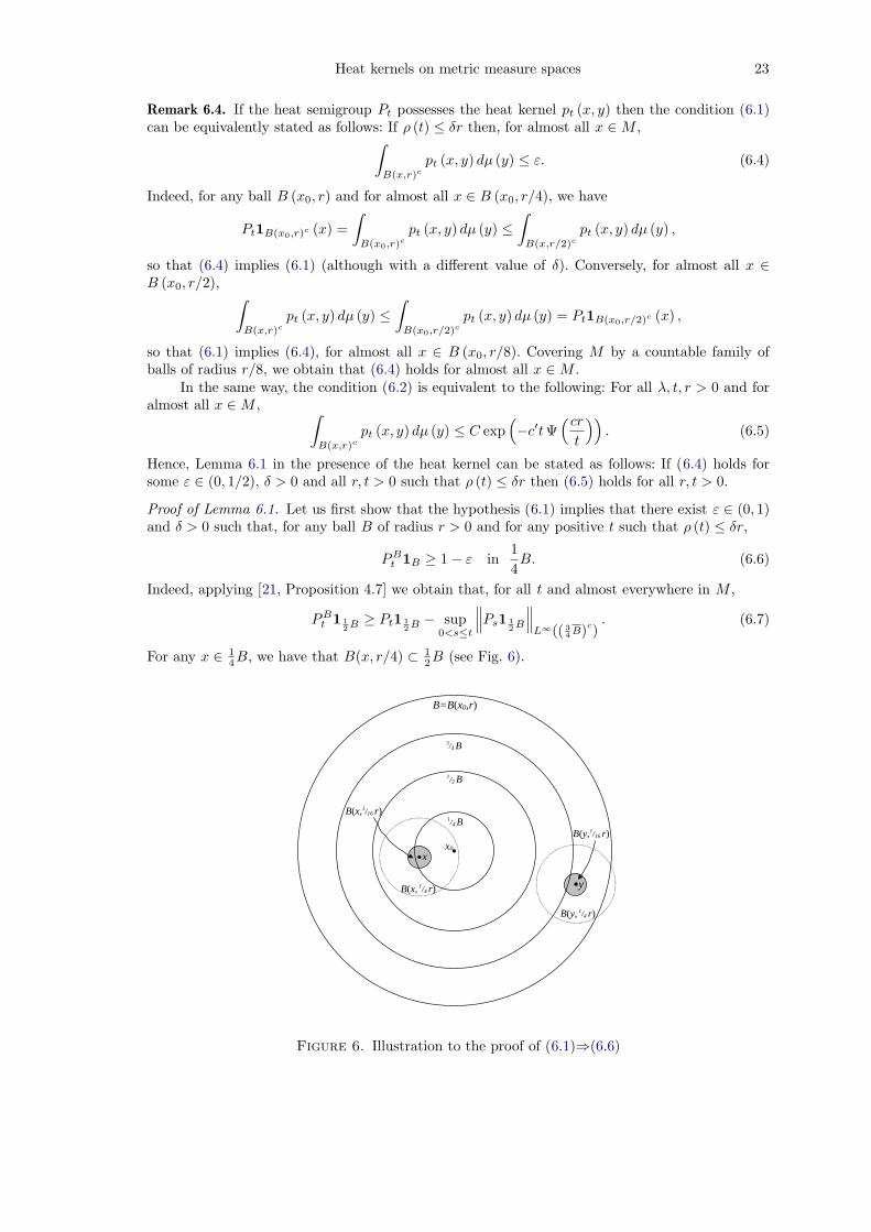
Remark 6.4. If the heat semigroup Pt possesses the heat kernel pt (x, y) then the condition (6.1)can be equivalently stated as follows: If ρ (t) ≤ δr then, for almost all x ∈ M ,
∫
B(x,r)c
pt (x, y) dμ (y) ≤ ε. (6.4)
Indeed, for any ball B (x0, r) and for almost all x ∈ B (x0, r/4), we have
Pt1B(x0,r)c (x) =∫
B(x0,r)c
pt (x, y) dμ (y) ≤∫
B(x,r/2)c
pt (x, y) dμ (y) ,
so that (6.4) implies (6.1) (although with a different value of δ). Conversely, for almost all x ∈B (x0, r/2),
∫
B(x,r)c
pt (x, y) dμ (y) ≤∫
B(x0,r/2)c
pt (x, y) dμ (y) = Pt1B(x0,r/2)c (x) ,
so that (6.1) implies (6.4), for almost all x ∈ B (x0, r/8). Covering M by a countable family ofballs of radius r/8, we obtain that (6.4) holds for almost all x ∈ M .
In the same way, the condition (6.2) is equivalent to the following: For all λ, t, r > 0 and foralmost all x ∈ M , ∫
B(x,r)c
pt (x, y) dμ (y) ≤ C exp(−c′t Ψ
(cr
t
)). (6.5)
Hence, Lemma 6.1 in the presence of the heat kernel can be stated as follows: If (6.4) holds forsome ε ∈ (0, 1/2), δ > 0 and all r, t > 0 such that ρ (t) ≤ δr then (6.5) holds for all r, t > 0.
Proof of Lemma 6.1. Let us first show that the hypothesis (6.1) implies that there exist ε ∈ (0, 1)and δ > 0 such that, for any ball B of radius r > 0 and for any positive t such that ρ (t) ≤ δr,
PBt 1B ≥ 1 − ε in
14B. (6.6)
Indeed, applying [21, Proposition 4.7] we obtain that, for all t and almost everywhere in M ,
P Bt 1 1
2 B ≥ Pt1 12 B − sup
0<s≤t
∥∥∥Ps1 1
2 B
∥∥∥
L∞(( 34 B)c)
. (6.7)
For any x ∈ 14B, we have that B(x, r/4) ⊂ 1
2B (see Fig. 6).
x0
y
1/4 B
B=B(x0,r)
1/2 B
x
3/4 B
B(y, 1/4 r)
B(x, 1/4 r)
B(y,1/16 r)
B(x,1/16 r)
Figure 6. Illustration to the proof of (6.1)⇒(6.6)

24 Grigor’yan, Hu and Lau
Using the identity Pt1 = 1 we obtain, for any x ∈ 14B,
Pt1 12 B = 1 − Pt1( 1
2 B)c ≥ 1 − Pt1B(x,r/4)c .
Applying (6.1) for the ball B (x, r/4), we obtain
Pt1B(x,r/4)c ≤ ε in B (x, r/16) ,
provided t satisfies
ρ (t) ≤ δr
4. (6.8)
It follows that, for any x ∈ 14B,
Pt1 12 B ≥ 1 − ε in B (x, r/16) ,
whence
Pt1 12 B ≥ 1 − ε in
14B. (6.9)
On the other hand, for any y ∈(
34B)c
, we have 12B ⊂ B (y, r/4)c (see Fig. 6), whence
Ps1 12 B ≤ Ps1B(y,r/4)c .
Applying (6.1) for the ball B (y, r/4) at time s, we obtain if (6.8) holds then, for all 0 < s ≤ t,
Ps1B(y,r/4)c ≤ ε in B (y, r/16) .
It follows that, for any y ∈(
34B)c
,
Ps1 12 B ≤ ε in B (y, r/16) ,
whence
Ps1 12 B ≤ ε in
(34B
)c
. (6.10)
Combining (6.7), (6.9) and (6.10), we obtain that, under condition (6.8),
PBt 1B ≥ PB
t 1 12 B ≥ 1 − 2ε in
14B, (6.11)
which is equivalent to (6.6).Now we show that (6.6) implies (6.2). The proof will be split into 5 steps.Step 1. Assuming that
ρ (t) ≤ δr (6.12)
and that B is a ball of radius r, rewrite (6.6) in the form
1 − PBt 1B ≤ ε in
14B. (6.13)
For any positive integer k, set Bk = kB and we will prove that
1 − PBkt 1Bk
≤ εk in14B. (6.14)
Since M is separable, there is a countable dense set of points in Bk. Let {bj} be a sequence of ballsof radii r centered at those points. Clearly, bj ⊂ Bk+1 and the family
{14bj
}covers Bk (see Fig. 7).
Due to (6.12), inequality (6.6) is valid for any ball bj , that is, for all 0 < s ≤ t,
PBk+1s 1Bk+1 ≥ P bj
s 1bj ≥ 1 − ε in14bj .
It follows thatPBk+1
s 1Bk+1 ≥ 1 − ε in Bk.
Applying the inequality (5.13) of Corollary 5.6 with Ω = Bk+1 and U = Bk, we obtain that thefollowing inequality holds in Bk:
1 − PBk+1t 1Bk+1 ≤
(1 − PBk
t 1Bk
)sup
0<s≤t
∥∥1 − PBk+1
s 1Bk+1
∥∥
L∞(Bk)
≤ ε(1 − PBk
t 1Bk
).
Iterating in k and using (6.13), we obtain (6.14).

Heat kernels on metric measure spaces 25
Bk
Bk+1
bj
1/4bj
r
Figure 7. Balls {Bk} and {bj}
It follows from (6.14) that
Pt1Bck≤ 1 − Pt1Bk
≤ 1 − PBkt 1Bk
≤ εk in14B. (6.15)
Although (6.15) has been proved for any integer k ≥ 1, it is trivially true also for k = 0, if wedefine B0 := ∅.
Step 2. Fix t > 0, x ∈ M and consider the function
Et,x = exp
(
cd(x, ∙)ρ(t)
)
, (6.16)
where the constant c > 0 is to be determined later on. Set
r = δ−1ρ (t) ,
and we will prove that
Pt (Et,x) ≤ C in B (x, r/4) , (6.17)
where C is a constant depending on ε, δ. Set as before Bk = B (x, kr) , k ≥ 1, and B0 = ∅. Using(6.16) and (6.15), we obtain that in B (x, r/4),
Pt (Et,x) =∞∑
k=0
Pt
(1Bk+1\Bk
Et,x
)
≤∞∑
k=0
‖Et,x‖L∞(Bk+1)Pt
(1Bk+1\Bk
)
≤∞∑
k=0
exp
(
c(k + 1) r
ρ(t)
)
Pt
(1Bc
k
)
≤∞∑
k=0
exp(c(k + 1)δ−1
)εk.
Choosing c < δ log 1ε we obtain that this series converges, which proves (6.17).
Step 3. Let us prove that, for all t > 0 and x ∈ M ,
PtEt,x ≤ C1Et,x, (6.18)
26 Grigor’yan, Hu and Lau
for some constant C1 = C (ε, δ). Observe first that, for all y, z ∈ M , we have by the triangleinequality
Et,x(y) = exp
(
cd(x, y)ρ(t)
)
≤ exp
(
cd(x, z)ρ(t)
)
exp
(
cd(z, y)ρ(t)
)
= Et,x(z)Et,z(y),
which can also be written in the form of a function inequality:
Et,x ≤ Et,x (z) Et,z.
It follows thatPt (Et,x) ≤ Et,x (z) Pt (Et,z) . (6.19)
By the previous step, we havePt (Et,z) ≤ C in B (z, r) , (6.20)
where r = 14δ−1ρ (t). For all y ∈ B (z, r), we have
Et,z (y) ≤ exp
(cr
ρ (t)
)
= exp(cδ−1/4
)=: C ′,
whenceEt,x (z) ≤ Et,x (y) Et,z (y) ≤ C ′Et,x (y) .
Letting y vary, we can writeEt,x (z) ≤ C ′Et,x in B (z, r) .
Combining this with (6.19) and (6.20), we obtain
Pt (Et,x) ≤ CC ′Et,x in B (z, r) .
Since z is arbitrary, covering M by a countable sequence of balls like B (z, r), we obtain that (6.18)holds on M with C1 = CC ′.
Step 4. Let us prove that, for all t > 0, x ∈ M , and for any positive integer k,
Pkt (Et,x) ≤ Ck1 in
14B, (6.21)
where B =(x, δ−1ρ (t)
). Indeed, by (6.18)
Pkt (Et,x) = P(k−1)tPt (Et,x) ≤ C1P(k−1)tEt,x
which implies by iteration thatPkt (Et,x) ≤ Ck−1
1 PtEt,x.
Combining with (6.17) and noticing that C ≤ C1, we obtain (6.21).Step 5. Fix a ball B = B (x0, r) and observe that (6.2) is equivalent to the following: for all
t, λ > 0,
Pt1Bc ≤ C exp
(
c′λt −cr
ρ(1/λ)
)
in12B, (6.22)
where C, c, c′ > 0 are constants depending on ε, δ. In what follows, we fix also t and λ.Observe first that, for any x ∈ 1
2B,
Pt1Bc ≤ Pt1B(x,r/2)c .
Hence, it suffices to prove that, for any x ∈ 12B,
Pt1B(x,r/2)c ≤ C exp
(
c′λt −cr
ρ(1/λ)
)
(6.23)
in a (small) ball around x. Covering then 12B by a countable family of such balls, we then obtain
(6.22).Changing t to t/k in (6.21), we obtain that
Pt
(Et/k,x
)≤ Ck
1 in B (x, σk)

Heat kernels on metric measure spaces 27
where σk = 14δ−1ρ (t/k). Since
Et/k,x ≥ exp
(
cr
ρ (t/k)
)
in B (x, r)c
and, hence,
1B(x,r)c ≤ exp
(
−cr
ρ(t/k)
)
Et/k,x,
we obtain that the following inequality holds in B (x, σk)
Pt1B(x,r)c ≤ exp
(
−cr
ρ(t/k)
)
Pt
(Et/k,x
)≤ exp
(
c′k −cr
ρ(t/k)
)
where c′ = log C1. Given λ > 0, choose an integer k ≥ 1 such that
k − 1t
< λ ≤k
t.
Then we obtain the following inequality in B (x, σk)
Pt1B(x,r)c ≤ exp
(
c′ (λt + 1) −cr
ρ (1/λ)
)
, (6.24)
which finishes the proof. �
6.2. Consequences of two-sided estimates (local case)
Now we are able to specify the local case in the statement of Theorem 4.9.Given two points x, y ∈ M , a chain connecting x and y is any finite sequence {xk}
nk=0 of
points in M such that x0 = x, xn = y. We say that a metric space satisfies the chain condition ifthere is a constant C > 0 such that for any positive integer n and for all x, y ∈ M there is a chain{xk}
nk=0 connecting x and y, such that
d (xk, xk+1) ≤ Cd (x, y)
nfor all k = 0, 1, ..., n − 1. (6.25)
For example, the geodesic distance on any length space satisfies the chain condition. On the otherhand, the combinatorial distance on a graph does not satisfy it.
Theorem 6.5. Assume that the metric measure space (M,d, μ) satisfies the chain condition andthat μ satisfies (VD) and (RVD). Let (E ,F) be a regular, local and conservative Dirichlet form,and let {pt} be the associated heat kernel such that, for all t > 0 and almost all x, y ∈ M ,
C ′1
V(x, t1/β
)Φ
(
C1d (x, y)t1/β
)
≤ pt (x, y) ≤C ′
2
V(x, t1/β
)Φ
(
C2d (x, y)t1/β
)
(6.26)
where C1, C′1, C2, C
′2 are positive constants, α, α′ are the exponents from (VD) and (RVD), respec-
tively, and β > α − α′. Then β ≥ 2 and the following inequality holds:
c′1 exp(−c1s
β/(β−1))≤ Φ(s) ≤ c′2 exp
(−c2s
β/(β−1))
(6.27)
for some positive constants c1, c′1, c2, c
′2 and all s > 0.
Proof. Let us first observe that the locality and the conservativeness imply the strong locality.Indeed, by [15, Lemma 4.5.2., p. 159 and Lemma , p. 161], we have the following identity
limt→0
1t
∫
M
(1 − Pt1) u2 dμ =∫
M
u2dk
for any u ∈ F where k is the killing measure of (E ,F) and u is a quasi-continuous version of u.Since Pt1 = 1, it follows that k = 0. Therefore, by the Beurling-Deny formula [15, Theorem 3.2.1,p.108], (E ,F) is strongly local. This will allow us to apply later Lemma 6.1.
We split the further proof into five steps.Step 1. By Lemma 4.3 and the lower bound of pt, we obtain
Φ(s) ≤ c(1 + s)−(α′+β) for all s > 0.
28 Grigor’yan, Hu and Lau
Therefore, using the upper bound of pt, we obtain (similar to (4.15)) that∫
B(x,r)c
pt(x, y)dμ(y) ≤ c
∫ ∞
12 r/t1/β
sα−1Φ(s)ds
≤ c′∫ ∞
12 r/t1/β
sα−α′−β−1ds.
Due to the condition β > α−α′, the integral in the right hand side converges and, hence, the righthand side can be made arbitrarily small provided rt−1/β is large enough. We conclude by Lemma6.1 (cf. Remark 6.4) with ρ(t) = t1/β that, for all r, t > 0 and for almost all x ∈ M ,
∫
B(x,r)c
pt (x, y) dμ (y) ≤ C exp(−c′t Ψ
(cr
t
)), (6.28)
whereΨ(s) := sup
λ>0
{sλ1/β − λ
}. (6.29)
Step 2. Let us prove that β > 1. If β < 1 then it follows from (6.29) that Ψ ≡ ∞. Substitutinginto (6.28) and letting r → 0, we obtain that, for almost all x ∈ M ,
∫
M\{x}pt (x, y) dμ (y) = 0.
It follows from the stochastic completeness that there is a point x ∈ M of a positive measure,which contradicts Remark 4.4.
Assume now that β = 1. Then by (6.29)
Φ (s) =
{0, 0 ≤ s ≤ 1∞, s > 1,
which implies that, for all t < cr and for almost all x ∈ M ,∫
B(x,r)c
pt (x, y) dμ (y) = 0,
that is, pt (x, y) = 0 for all t < cd (x, y) and almost all x, y ∈ M . Together with (6.26), this yieldsthe following bounds of the heat kernel for all t > 0 and almost all x, y ∈ M :
C−1
V(x, t1/β
)Φ
(d (x, y)t1/β
)
≤ pt (x, y) ≤C
V(x, t1/β
) Φ
(d (x, y)t1/β
)
(6.30)
where
Φ (s) =
{Φ(s) , s ≤ c−1
0, s > c−1.
Clearly, the functions Φ and Φ satisfy the hypotheses of Theorem 4.7. We conclude by Theorem4.7 that β = β∗ whereas by Lemma 3.1 β∗ ≥ 2, which contradicts to β = 1.
Step 3. Using that β > 1, let us show that the heat kernel satisfies the following upper bound
pt(x, y) ≤C
V (x, t1/β)exp
(
−c
(d (x, y)t1/β
)β/(β−1))
. (6.31)
Setting in (6.29) λ = (s/β)β
β−1 we obtain as in Remark 6.3
Ψ (s) = cβsβ/(β−1)
so that (6.28) becomes∫
B(x,r)c
pt (x, y) dμ (y) ≤ C exp
(
−c( r
t1/β
)β/(β−1))
. (6.32)
On the other hand, by the upper bound in (6.26), we have, for all t > 0 and almost all x, y ∈ M ,
pt (x, y) ≤C
V(x, t1/β
) . (6.33)
Heat kernels on metric measure spaces 29
Setting r = 12d (x, y), we obtain from (6.32) and (6.33) that
p2t(x, y) =∫
M
pt(x, z)pt(z, y) dμ(z)
≤∫
B(x,r)c
pt(x, z)pt(z, y) dμ(z) +∫
B(y,r)c
pt(x, z)pt(z, y) dμ(z) (6.34)
≤C
V(y, t1/β
)∫
B(x,r)c
pt(x, z) dμ(z)
+C
V(x, t1/β
)∫
B(y,r)c
pt(y, z) dμ(z)
≤
(C
V(y, t1/β
) +C
V(x, t1/β
)
)
exp
(
−c( r
t1/β
)β/(β−1))
. (6.35)
By (VD) we have
V(x, t1/β
)
V(y, t1/β
) ≤ C
(d (x, y) + t1/β
t1/β
)α
= C(1 +
r
t1/β
)α
.
Absorbing the polynomial function of r/t1/β into the exponential term in (6.35), we obtain (6.31).Step 4. Now we can prove that β ≥ 2. Indeed, we have the estimate (6.30) where this time
Φ(s) = exp(−csβ/(β−1)
).
Since the estimate (6.30) satisfies the hypotheses Theorem 4.7, we obtain β ≥ 2 by the sameargument as in Step 2.
Step 5. The lower bound in (6.30) implies that, for all t > 0 and almost all x, y ∈ M , suchthat d (x, y) ≤ s0t
1/β ,
pt (x, y) ≥c
V (x, t1/β). (6.36)
Let us show that this implies the following lower bound
pt(x, y) ≥c
V (x, t1/β)exp
(
−C
(d (x, y)t1/β
)β/(β−1))
, (6.37)
for all t > 0 and almost all x, y ∈ M . Iterating the semigroup identity, we obtain for any positiveinteger n and real r > 0
pt(x, y) =∫
M
...
∫
M
p tn(x, z1)p t
n(z1, z2)...p t
n(zn−1, y)dμ(zn−1)...dμ(z1)
≥∫
B(x1,r)
...
∫
B(xn−1,r)
p tn(x, z1)p t
n(z1, z2)...p t
n(zn−1, y)dμ(zn−1)...dμ(z1), (6.38)
where {xi}ni=0 is a chain connecting x and y that satisfies (6.25) (see Fig. 8).
Denote for simplicity z0 = x and zn = y. Setting
r =d(x, y)
n(6.39)
and noticing that zi ∈ B(xi, r), 0 ≤ i ≤ n − 1, we obtain by the triangle inequality and (6.25)
d(zi, zi+1) ≤ d(xi, xi+1) + 2r ≤ C ′ d(x, y)n
where C ′ = C + 2. Next, we would like to use (6.36) to estimate pt/n (zi, zi+1) from below. Forthat, the following condition must be satisfied:
d (zi, zi+1) ≤ s0
(t
n
)1/β
,
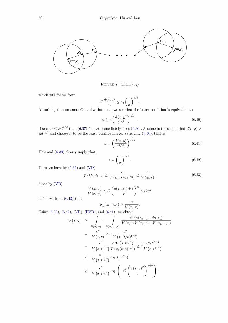
30 Grigor’yan, Hu and Lau
x=x0
x1x2 y=xn
xn-1
Figure 8. Chain {xi}
which will follow from
C ′ d(x, y)n
≤ s0
(t
n
)1/β
.
Absorbing the constants C ′ and s0 into one, we see that the latter condition is equivalent to
n ≥ c
(d (x, y)t1/β
) ββ−1
. (6.40)
If d(x, y) ≤ s0t1/β then (6.37) follows immediately from (6.36). Assume in the sequel that d(x, y) >
s0t1/β and choose n to be the least positive integer satisfying (6.40), that is
n �
(d (x, y)t1/β
) ββ−1
(6.41)
This and (6.39) clearly imply that
r �
(t
n
)1/β
. (6.42)
Then we have by (6.36) and (VD)
p tn(zi, zi+1) ≥
c
V(zi, (t/n)1/β
) ≥c
V (zi, r). (6.43)
Since by (VD)V (zi, r)V (xi, r)
≤ C
(d(zi, xi) + r
r
)α
≤ C2α,
it follows from (6.43) that
p tn(zi, zi+1) ≥
c
V (xi, r).
Using (6.38), (6.42), (VD), (RVD), and (6.41), we obtain
pt(x, y) ≥∫
B(x1,r)
...
∫
B(xn−1,r)
cndμ(zn−1)...dμ(z1)V (x, r) V (x1, r) ...V (xn−1, r)
=cn
V (x, r)≥ c′
cn
V(x, (t/n)1/β
)
=c′
V(x, t1/β
)cnV
(x, t1/β
)
V(x, (t/n)1/β
) ≥ c′cnnα′/β
V(x, t1/β
)
≥c′
V(x, t1/β
) exp (−Cn)
≥c′
V(x, t1/β
) exp
−C
(d (x, y)β
t
) 1β−1
.

Heat kernels on metric measure spaces 31
Comparing (6.26) with (6.31) and (6.37), we obtain (6.27). �
Corollary 6.6. Under the hypotheses of Theorem 6.5, we have E (u) � Eβ (u) for all u ∈ L2 (M).Consequently, F = W β/2,2.
Proof. Indeed, by Lemma 4.2 we have E (u) ≥ cEβ (u). Using the upper bound (6.31) and Lemma(4.5), we obtain E (u) ≤ CEβ (u), which finishes the proof. �
References
[1] D.G. Aronson, Non-negative solutions of linear parabolic equations Ann. Scuola Norm. Sup. Pisa. Cl.Sci. (4) 22 (1968), 607–694. Addendum 25 (1971), 221–228.
[2] M.T. Barlow, Diffusions on fractals, Lect. Notes Math. 1690, Springer, 1998, 1-121.
[3] M.T. Barlow and R.F. Bass, Brownian motion and harmonic analysis on Sierpınski carpets, Canad.J. Math. (4) 51 (1999), 673-744.
[4] M.T. Barlow, R.F. Bass, Z.-Q. Chen and M. Kassmann, Non-local Dirichlet forms and symmetricjump processes, Trans. Amer. Math. Soc. 361 (2009), 1963-1999.
[5] M. Barlow, T. Coulhon and T. Kumagai, Characterization of sub-Gaussian heat kernel estimates onstrongly recurrent graphs, Comm. Pure Appl. Math., 58 (2005), 1642-1677.
[6] M.T. Barlow and E.A. Perkins, Brownian motion on the Sierpınski gasket, Probab. Theory. RelatedFields 79 (1988), 543-623.
[7] A. Bendikov and L. Saloff-Coste, On-and-off diagonal heat kernel behaviors on certain infinite dimen-sional local Dirichlet spaces, Amer. J. Math. 122 (2000), 1205–1263.
[8] G. Carron, Inegalites isoperimetriques de Faber-Krahn et consequences, in: Actes de la table ronde degeometrie differentielle (Luminy, 1992) Collection SMF Seminaires et Congres, 1 (1996), 205–232.
[9] E.A. Carlen and S. Kusuoka and D.W. Stroock, Upper bounds for symmetric Markov transitionfunctions, Ann. Inst. Henri. Poincare-Probab. Statist. 23(1987), 245-287.
[10] I. Chavel, Eigenvalues in Riemannian geometry, Academic Press, New York, 1984.
[11] T. Coulhon, Ultracontractivity and Nash type inequalities, J. Funct. Anal. 141 (1996), 510-539.
[12] T. Coulhon, Heat kernel and isoperimetry on non-compact Riemannian manifolds, in: Heat kernelsand analysis on manifolds, graphs, and metric spaces, 65–99, Contemp. Math., 338 Amer. Math. Soc.,Providence, RI, 2003.
[13] M. Cowling and S. Meda, Harmonic analysis and ultracontractivity. Trans. Amer. Math. Soc. 340(1993), 733–752.
[14] E.B. Davies, Heat kernels and spectral theory, Cambridge University Press, 1989.
[15] M. Fukushima and Y. Oshima Y. and M. Takeda, Dirichlet forms and symmetric Markov processes,De Gruyter, Studies in Mathematics, 1994.
[16] M. Fukushima and T. Shima, On a spectral analysis for the Sierpinski gasket. Potential Anal. 1 (1992),1–35.
[17] A. Grigor’yan, Heat kernel upper bounds on a complete non-compact manifold, Rev. Mat. Iberoamer-icana 10(1994), 395–452.
[18] A. Grigor’yan, Estimates of heat kernels on Riemannian manifolds, London Math. Soc. Lecture NoteSer., 273 (1999),140-225.
[19] A. Grigor’yan, Heat kernels on metric measure spaces, to appear in ”Handbook of Geometric AnalysisNo.2” (ed. L. Ji, P. Li, R. Schoen, L. Simon), Advanced Lectures in Math., IP.
[20] A. Grigor’yan and J. Hu, Off-diagonal upper estimates for the heat kernel of the Dirichlet forms onmetric spaces, Invent. Math. 174 2008, 81–126.
[21] A. Grigor’yan and J. Hu, Upper bounds of heat kernels on doubling spaces, preprint 2008.
[22] A. Grigor’yan, J. Hu and K.-S. Lau, Heat kernels on metric-measure spaces and an application tosemilinear elliptic equations, Trans. Amer. Math. Soc. 355 (2003), 2065–2095.
[23] A. Grigor’yan, J. Hu and K.-S. Lau, Equivalence conditions for on-diagonal upper bounds of heatkernels on self-similar spaces, J. Func. Anal. 237 (2006), 427-445.
[24] A. Grigor’yan and T. Kumagai, On the dichotomy in the heat kernel two sided estimates. In: Analysison Graphs and its Applications (P. Exner et al. (eds.)), Proc. of Symposia in Pure Math. 77, pp.199–210, Amer. Math. Soc. 2008.
32 Grigor’yan, Hu and Lau
[25] A. Grigor’yan and A. Telcs, Sub-Gaussian estimates of heat kernels on infinite graphs, Duke Math. J.109(2001), 451–510.
[26] B.M. Hambly and T. Kumagai, Transition density estimates for diffusion processes on post criticallyfinite self-similar fractals, Proc. London Math. Soc. (3)79 (1999), 431-458.
[27] W. Hebisch and L. Saloff-Coste, On the relation between elliptic and parabolic Harnack inequalities,Ann. Inst. Fourier (Grenoble) 51 (2001), 1437-1481.
[28] A. Jonsson, Brownian motion on fractals and function spaces, Math. Zeit. 222 (1996), 495-504.
[29] J. Jorgenson and W. Lynne, ed. The ubiquitous heat kernel. Contemporary Math. 398, AMS, 2006.
[30] J. Kigami, Analysis on fractals, Cambridge University Press, Cambridge, 2001.
[31] J. Kigami, Local Nash inequality and inhomogenous of heat kernels, Proc. London Math. Soc. 89(2004), 525–544.
[32] P.Li and S.T. Yau, On the parabolic kernel of the Schrodinger operator, Acta Math. 156(1986), 153-201.
[33] J. Nash, Continuity of solutions of parabolic and elliptic equations, Amer. J. Math. 80 (1958), 931-954.
[34] K. Pietruska-Pa luba, On function spaces related to fractional diffusion on d-sets, Stochastics andStochastics Reports, 70 (2000), 153-164.
[35] F.O. Porper and S.D. Eidel’man, Two-side estimates of fundamental solutions of second-order para-bolic equations and some applications, Russian Math. Surveys, 39 (1984), 119-178.
[36] L. Saloff-Coste, Aspects of Sobolev-type inequalities, Cambridge University Press, Cambridge, 2002.
[37] L. Saloff-Coste, A note on Poincare, Sobolev, and Harnack inequalities, Internat. Math. Res. Notices1992, no. 2, 27–38.
[38] R. Schoen and S.-T Yau, Lectures on Differential Geometry, International Press, 1994.
[39] D.W. Stroock, Estimates on the heat kernel for the second order divergence form operators, in: Proba-bility theory. Proceedings of the 1989 Singapore Probability Conference held at the National Universityof Singapore, June 8-16 1989, ed. L.H.Y. Chen, K.P. Choi, K. Hu and J.H. Lou, Walter De Gruyter,1992, 29-44.
[40] M. Tomisaki, Comparison theorems on Dirichlet norms and their applications, Forum Math. 2 (1990),277–295.
[41] N.Th. Varopoulos, Hardy-Littlewood theory for semigroups, J. Funct. Anal. 63 (1985), 240-260.
[42] N. Th. Varopoulos and L. Saloff-Coste and T. Coulhon, Analysis and geometry on groups, CambridgeTracts in Mathematics, 100. Cambridge University Press, Cambridge, 1992.
[43] F.-Y. Wang, Functional inequalities for empty essential spectrum, J. Funct. Anal. 170 (2000), 219-245.
Alexander Grigor’yanFakultat fur Mathematik, Universitat Bielefeld, Postfach 100131, 33501 Bielefeld, Germany.e-mail: [email protected]
Jiaxin HuDepartment of Mathematical Sciences, Tsinghua University, Beijing 100084, China.e-mail: [email protected]
Ka-Sing LauDepartment of Mathematics, the Chinese University of Hong Kong, Shatin, N.T., Hong Kong.e-mail: [email protected]


![A Kernel Classification Framework for Metric Learningcslzhang/paper/SVMML.pdf · kernel learning, and proposed a framework for metric learning with multiple kernels [21]. In our](https://static.fdocuments.in/doc/165x107/5fcc922fcbb0c45e3b76fd9e/a-kernel-classiication-framework-for-metric-cslzhangpapersvmmlpdf-kernel.jpg)