ABSTRACT

STUDY OF HEAT FLUX GAGES USING SENSITIVITY ANALYSIS'

Kevin J. Dowding, Ben F. Blackwell, and Robert J. Cochran

Thermal Sciences Department 91 13, M/S 0835 Sandia National Laboratories

Albuquerque, New Mexico, 871 85-0835

The response and operation of a heat flux gage is studied using sensitivity analysis. Sensitivity analysis is the process by which one determines the sensitivity of a model output to changes in the model parameters. This process uses sensitivity coefficients that are defined as partial derivatives of field variables - e.g., temperature - with respect to model parameters - e.g., thermal properties and boundary conditions). Computing sensitivity coefficients, in addition to the response of a heat flux gage, aids in identifying model parameters that significantly impact the temperature response. A control volume, finite element- based code is used to implement numerical sensitivity coefficient calcu- lations, allowing general problems to be studied. Sensitivity coeffi- cients are discussed for the well known Gardon gage.

NOMENCLATURE

a C e"'

h k L 4' 4

area, in2 volumetric heat capacity, JIm3K volumetric source, w/m3 convection coefficient, WIm2K thermal conductivity, WImK length of Gardon gage, rn heat flux, W/m2 heat flux vector, W/m2

1. Sandia is a rnultiprogram laboratory operated by Sandia Corporation, a Lockheed Martin Company, for the United States Department of Energy under Contract DE-AC/o4-94AL85000.

boundary heat flux, W/m2 radius of Gardon gage, m temperature, K initial temperature, K temperature at center of Gardon gage, K scaled temperature sensitivity coefficient for parameter p , K convection temperature, K

volume, rn3 spatial coordinates

Greek: c1 thermal diffusivity, m2/s P parameter 6 E emissivity

oP oT P density, kg/ rn3

thickness of Gardon gage, rn

standard deviation of parameter p standard deviation of temperature, K

Subscripts b boundary B base (copper) f foil (constantan) W wire (copper)

TER

DISCLAIMER

This report was prepared as an account of work sponsored by an agency of the United States Government. Neither the United States Government nor any agency thereof, nor any of their employees. makes any warranty, express or implied, or assumes any legal liability or responsibility for the accuracy, completeness, or use- fulness of any information, apparatus, product, or process disclosed, or represents that its use would not infringe privately owned rights. Reference herein to any spe- cific commercial product, process, or service by trade name, trademark, manufac- turer, or otherwise does not necessarily constitute or imply its endorsement, m m - menbtion, or favoring by the United States Government or any agency thereof. The views and opinions of authors expressed herein do not necMsariiy state or reflect those of the United States Government or any agency thereof.

DISCLAIMER

Portions of this document may be illegible in electronic image products. Images are produced from the best available original document.

INTRODUCTION

Sensitivity analysis is an important and useful analysis tool. Sensi- tivity analysis means that the partial derivative of the state variable (temperature for thermal problems) with respect to physical model parameters (thermal conductivity, volumetric heat capacity, convection coefficient, emissivity, etc.) is calculated. This partial derivative is called a sensitivity coefficient. Valuable insight is gleaned from sensi- tivity coefficients. Sensitivity coefficient use and computation is dis- cussed in this paper. In particular it is demonstrated how sensitivity coefficients can provide information concerning the effect of parame- ters on the response of heat flux gages. The insight from the sensitivity analysis can aid in gage design and improve our understanding of the gage’s response. With a better understanding of the measured response, and more importantly what factors are influential on the response, more accurate data reduction can be achieved. Data reduction refers to the analysis relating the gage’s measured response to the incident surface or absorbed heat flux.

Under certain circumstances data reduction for the heat flux gages involves an algebraic relationship between the measured response and heat flux. This relationship occurs because the response can be analyti- cally calculated. When the assumptions for the simple relationship are not valid, inverse techniques may be needed. Inverse techniques allow a complex model, such as a finite element model, to be used in conjunc- tion with measurements to estimate parameters or functions in the model that cannot be measured. In practice the heat flux gage predicts the heat flux at the surface of the gage from a measured temperature response. This problem is the classic inverse heat conduction problem (IHCP), Beck et al. (1985). The IHCP has added difficulty due to its ill- posed nature. Sensitivity coefficients are key to understanding how the measured response can be used to estimate the heat flux and possibly other parameters.

The importance of observing sensitivity coefficients has been widely advocated in parameter estimation by Beck; see Beck and Arnold (1977), Beck (1970), and Beck (1996). Other researchers have also used sensitivity coefficients to derive insight for parameter estima- tion; see Dowding et al. (1998), Marchall and Milos (1997), and Vozar and Sramkova (1997). Their use to designing an optimal parameter estimation experiment is discussed in Beck and Arnold (1977, Chapter 8); Taktak et al. (1993); and Emery and Fadale (1990,1996, and 1997). Moffat (1985 and 1982) has suggested sensitivity coefficients be com- puted in analysis codes to quantify the experimental uncertainty associ- ated with complex analyses. It is straightforward to compute experimental uncertainty and propagate error through an analysis code using perturbation methods when sensitivity coefficients are available.

Measuring the heat flux emanating from a radiative and/or convec- tive source, such as a fire, is difficult. A common measurement approach uses a device that relates an easily measured response to the incident surface heat flux. A device that applies this approach is the cir- cular foil, or Gardon gage, (Gardon, 1953). Gardon’s original paper described the theory of operation for the Gardon gage. Since then, sev- eral investigations have studied the influence of heat loss modes ini- tially neglected by Gardon; see Malone (1967), Kirchhoff (1972), Bore11 and Diller (1987), and Kuo and Kulkarni (1991). Additionally, Ash (1969) and Keltner and Wildin (1972) investigated the time response of the gage, which was initially assumed exponential in time by Gardon (1 953).

Previously noted studies have demonstrated the influence of an effect - for example, heat losses by natural convection - on the response of the gage. To address the significance of an effect, the gage’s response is often compared to the response neglecting the effect. Sensitivity coefficients provide a means to quantify the significance of an effect on the response but in reference to other physical model effects. This pro- vides two insights. First, it allows physical effects in the model to be ranked according to importance. Second, it shows how dependent the response is on the parameters in the model. From a design standpoint it is essential to minimize the dependence on parameters that are least understood. When this is not feasible, efforts to better understand the parameters should be started. With the simplistic design of the Gardon gage, many insightful analytical models have been developed. The numerical solution studied in this paper permits a more general study of all the relevant physics. The addition of sensitivity coefficients to a numerical solution greatly enhances the value of the results.

In this paper sensitivity coefficients are used as an analysis tool to develop insight into the operation of heat flux gages. In the following section sensitivity coefficients and sensitivity equations are described. Sensitivity coefficients for a Gardon gage are presented and discussed in the subsequent section. Insight derived from sensitivity coefficients is described. A summary concludes the paper.

SENSITIVITY COEFFICIENTS

Definition Although there are other dependent variable for which sensitivity

is important, sensitivity coefficients related to temperature are studied in this paper. The sensitivity coefficient is the partial derivative of tem- perature with respect to a parameter, which is aT/ap for a parameter p. Scaling allows sensitivity coefficients for different parameters to be compared. A scaled (sometimes called “modified”) sensitivity coeffi- cient is:

Some papers represent the sensitivity coefficient for parameter p with Xp In this paper it is represented as Tp because it has units of tempera- ture, allowing sensitivity coefficient magnitudes for different parame- ters to be directly compared to temperature scales - e.g., magnitude of the transient temperature rise - within the problem.

Sensitivitv Coefficients for Comdex Problems Complex problems with irregular geometry or multiple materials

are generally solved with a numerical method. Several options exist to compute sensitivity coefficients with a numerical method. Blackwell et al. (1998) discuss the options and their implementation. The approach in this paper derives sensitivity equations by differentiating the describ- ing equations and numerically solving the resulting equations. The details of the procedure are presented in Blackwell et al. (1998). Equa- tions for temperature and sensitivity to parameters in the describing dif- ferential equation are discussed. The resulting equations are solved with a control volume finite element method with fully implicit time

integration (Hogan et al., 1994); this procedure is not discussed in the paper.

Parameters in Differential Eauation/Boundarv Condi- tion. The integral form of the energy equation for a heat conducting body is:

where the heat flux vector for isotropic thermal conductivity is given by Fourier’s Law,

4 = -kVT. (3)

The boundary condition, assuming only a specified flux in this case, is

where is along the boundary and

In Eq. (5) the specified heat flux is comprised of constant and convec- tive components.

Sensitivity equations are obtained by differentiating the energy equation, Eq. (2) through Eq. (3, with respect to a parameter and mul- tiplying the result by the parameter, The sensitivity equation for isotro- pic conductivity is

with boundary condition

(7)

In Eq. (6) to Eq. (S), the scaled sensitivity coefficient for thermal con- ductivity is

(9)

All thermal properties in Eq. (2) through Eq. (8) are assumed constant. Blackwell et al. (1998) discuss sensitivity equations for several other parameters and give a detailed derivation for sensitivity equations.

The right side term in Eq. (6), the sensitivity equation for conduc- tivity, is the only nonhomogeneous term in the problem. It is the driving or forcing term for the sensitivity problem and contains the tempera- ture. It is assumed that the temperature solution is already known, and the forcing term can be calculated. The forcing term is similar to a vol-

umetric sourcdsink with magnitude equal to the negative of the heat flux. It is the gradient of heat flux that is important because large but equal values of heat flux across a control volume produce a zero net contribution. This dependence is more obvious after applying the diver- gence theorem to the right side of Eq. (6)

( I [ k V T ] . d a = I ( I ( V . [kVT])dV = - I I I ( V . $)dz’ . (10) a ‘v ‘v

This equation demonstrates that the sensitivity coefficient for conduc- tivity is indicative of heat flux gradients. A large heat flux gradient means the conductivity is restricting heat transfer by conduction and influencing the temperature. The sensitivity coefficient for conductivity is large in this case. The converse is not necessarily true, however. That is, a small sensitivity coefficient for conductivity does not necessarily mean its effect on temperature is insignificant. Rather it indicates that temperature is not sensitive to changes about the mean value of conduc- tivity.

Temperature sensitivity does not provide complete information for the influence of conductivity. Heat flux sensitivity is especially perti- nent in the operation of heat flux gages. Application of Fourier’s Law gives heat flux sensitivity as

Computing heat flux sensitivity requires postprocessing the tempera- ture and temperature sensitivity. The first term on the right side is only nonzero for P = k and is the heat flux for this case. For all other param- eters the right side only contains the gradient of the sensitivity coeffi- cients.

Parameters in the Boundarv Condition. Sensitivity to parameters in the boundary conditions, such as a convection coefficient, convection temperature, etc., provide valuable insight as well. The sen- sitivity equation and boundary conditions for the convection coefficient are

- j j j ( C T , ) d V + j ] ( - k V T , ) . a da = 0

at ‘v a

- (kVT,) . d a = ( h g ) R . 6a ab a b

In contrast to the sensitivity equations for thermal properties, the sensi- tivity equation for the convection coefficient, Eq. (12), is homogeneous. However, the boundary condition in Eq. (13) and Eq. (14) is not homo- geneous. It contains an inhomogenous term (last term on the right side) that is identical to the boundary heat flux due to convection for temper- ature, Eq. (5) . When heat flux due to convection is large, the sensitivity to convection coefficient is correspondingly large. Hence sensitivity to the convection coefficient shows the importance of boundary heat transfer due to convection. Similarly the sensitivity equations for a

hf' T-, f( both sides of foil)

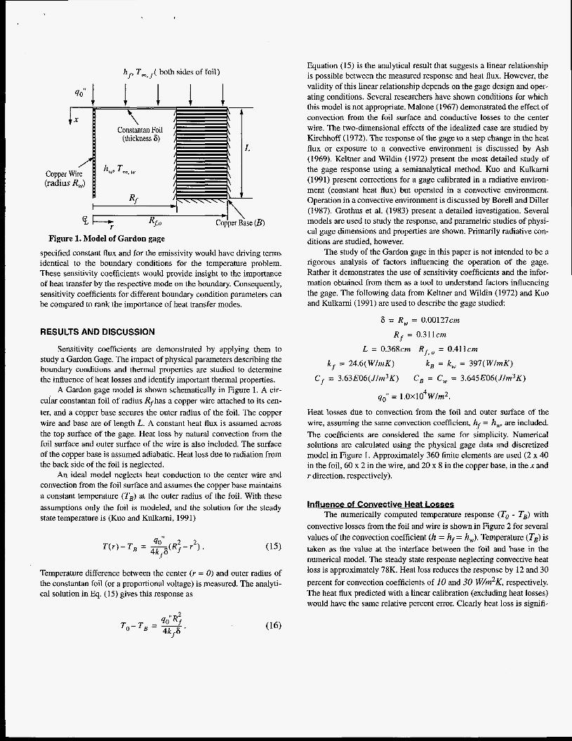
\ %I-- r RJCO Cgper Base (B) Figure 1. Model of Gardon gage

specified constant flux and for the emissivity would have driving terms identical to the boundary conditions for the temperature problem. These sensitivity coefficients would provide insight to the importance of heat transfer by the respective mode on the boundary. Consequently, sensitivity coefficients for different boundary condition parameters can be compared to rank the importance of heat transfer modes.

RESULTS AND DISCUSSION

Sensitivity coefficients are demonstrated by applying them to study a Gardon Gage. The impact of physical parameters describing the boundary conditions and thermal properties are studied to determine the influence of heat losses and identify important thermal properties.

A Gardon gage model is shown schematically in Figure 1. A cir- cular constantan foil of radius Rfhas a copper wire attached to its cen- ter, and a copper base secures the outer radius of the foil. The copper wire and base are of length L. A constant heat flux is assumed across the top surface of the gage. Heat loss by natural convection from the foil surface and outer surface of the wire is also included. The surface of the copper base is assumed adiabatic. Heat loss due to radiation from the back side of the foil is neglected.

An ideal model neglects heat conduction to the center wire and convection from the foil surface and assumes the copper base maintains a constant temperature (TB) at the outer radius of the foil. With these assumptions only the foil is modeled, and the solution for the steady state temperature is (Kuo and Kulkarni, 1991)

Temperature difference between the center (r = 0) and outer radius of the constantan foil (or a proportional voltage) is measured. The analyti- cal solution in Eq. (15) gives this response as

2 40"Rf

O - ,-4kf6' T T -

Equation (15) is the analytical result that suggests a linear relationship is possible between the measured response and heat flux. However, the validity of this linear relationship depends on the gage design and oper- ating conditions. Several researchers have shown conditions for which this model is not appropriate. Malone (1967) demonstrated the effect of convection from the foil surface and conductive losses to the center wire. The two-dimensional effects of the idealized case are studied by Kirchhoff (1972). The response of the gage to a step change in the heat flux or exposure to a convective environment is discussed by Ash (1969). Keltner and Wildin (1972) present the most detailed study of the gage response using a semianalytical method. Kuo and Kulkarni (1991) present corrections for a gage calibrated in a radiative environ- ment (constant heat flux) but operated in a convective environment. Operation in a convective environment is discussed by Bore11 and Diller (1987). Grothus et al. (1983) present a detailed investigation. Several models are used to study the response, and parametric studies of physi- cal gage dimensions and properties are shown. Primarily radiative con- ditions are studied, however.

The study of the Gardon gage in this paper is not intended to be a rigorous analysis of factors influencing the operation of the gage. Rather it demonstrates the use of sensitivity coefficients and the infor- mation obtained from them as a tool to understand factors influencing the gage. The following data from Keltner and Wildin (1972) and Kuo and Kulkami (1991) are used to describe the gage studied:

6 = R , = 0.00127cm

R f = 0.311cm

L = 0.368crn Rf, = 0.41 1 cm

kf = 24.6(W/mK) k , = k , = 397(W/mK)

C, = C, = 3.645E06(Jlm3K) Cf = 3.63E06(J/rn3K)

Heat losses due to convection from the foil and outer surface of the wire, assuming the same convection coefficient, hf = h, are included. The coefficients are considered the same for simplicity. Numerical solutions are calculated using the physical gage data and discretized model in Figure 1. Approximately 360 finite elements are used (2 x 40 in the foil, 60 x 2 in the wire, and 20 x 8 in the copper base, in the x and r direction, respectively).

Influence of Convective Heat Losses The numerically computed temperature response (To - TB) with

convective losses from the foil and wire is shown in Figure 2 for several values of the convection coefficient (h = h . = h,). Temperature (T,) is taken as the value at the interface between the foil and base in the numerical model. The steady state response neglecting convective heat loss is approximately 78K. Heat loss reduces the response by 12 and 30 percent for convection coefficients of 10 and 30 W/m2K, respectively. The heat flux predicted with a linear calibration (excluding heat losses) would have the same relative percent error. Clearly heat loss is signifi-

90 - 80 - 70 - 60 - 50 - 40 - 30 -

h = h - h , f - h = O

h = 10W/m2K .

h = 30W/m2K .

y, , . , , . . , , ~

'0 0.2 0.4 0.6 0.8 1 1.2 1.4 1.6 1.8 2 time, sec

Figure 2. Gardon gage temperature response

cant. Sensitivity coefficients are studied next to determine what param- eters influence the calculated response.

Sensitivity coefficients for the temperature difference (To - TB) are applicable for the Gardon gage. It can be shown that the sensitivity to a temperature difference is the difference of the sensitivity coefficients for the individual temperatures. It is noted that the sensitivity of tem- perature at the outer radius of the foil (TB) is approximately zero. Because temperature is nearly constant there, its value is insensitive to model parameters. Temperature sensitivity is exactly zero at a surface where temperature is prescribed.

Sensitivity coefficients are separated into two categories: those related to the boundary conditions and those related to thermal proper- ties. Dependence on the thermal properties can be eliminated with a careful calibration. However, the gage must be operated within the cali- bration bounds, which typically neglect convective heat loss.

-80 -60* 0 0.5 1 1.5 2

time, sec Figure 3. Sensitivity of Gardon gage temperature response to boundary condition parameters for h = 30W/m2K

Sensitivity to convection coefficients, ambient temperatures, and the applied heat flux is shown in Figure 3 for h = 3 0 W / m 2 K . The most influential parameter on the response is the applied heat flux q,," . Its value closely approximates the temperature response as seen in Figure 2. If the ideal model is applicable, Eq. (16), the scaled sensitiv- ity to the applied heat flux is identical to the steady state ideal tempera- ture response. This value is shown on the plot for comparison. By comparing the sensitivity to the applied heat flux with and without con- vective losses at steady state, the gage is shown to be less sensitive to the applied flux when there are convective losses.

Equal magnitudes are assumed for the convection coefficients describing heat losses from the foil and wire surfaces. However, sensi- tivity to the convection coefficients is markedly different. Sensitivity to the convection coefficient and ambient temperature for the foil (hf and T"$ are more than an order of magnitude larger than those for the wire (h, and T,J. Recall that the sensitivity equation for parameters in boundary conditions showed that these sensitivity coefficients are indicative of the importance of heat losses. The magnitudes indicate that the gage's response is influenced more by losses from the foil than by losses from the wire. The foil has a significantly larger surface area; thus losses from it are more important.

Sensitivities for the parameters describing losses from the foil are further discussed. Sensitivity to the convection coefficient (hf) is about 80 percent larger than sensitivity to the convection temperature (T,$). It is more important to know the convection coefficient than the ambi- ent temperature. The coefficients have different signs; sensitivity to hf is negative indicating an increase in this parameter results in an decrease in the temperature; sensitivity to T,,J is positive indicating an increase in this parameter results in a increase in the temperature. This is not to imply that the two effects may cancel each other.

Sensitivity to the thermal properties, thermal conductivity and vol- umetric heat capacity, of the foil and wire are shown in Figure 4. The properties of the foil have the largest sensitivity coefficients. Sensitivity

60 8or----l 4

I

40t *Ot

-800 -60: 0.5 1 1.5 2

time, sec

Figure 4. Sensitivity of Gardon gage temperature response to thermal properties for h = 30W/m2K

to the conductivity of the foil is maximum at steady state. Sensitivity to the heat capacity of the foil is maximum at approximately 0.25 seconds and decreases to zero at steady state. Thermal properties of the wire have small sensitivities. Small sensitivity indicates that the wire proper- ties are comparably less significant on the response of the gage. It does not necessarily mean the wire can be neglected in the model. Sensitiv- ity coefficients are computed for mean values of the parameters. A small sensitivity coefficient indicates that changes in the parameter, for the mean value of the parameters, have a small influence on the temper- ature. Although changes in the thermal properties of the wire are not significant, there could be appreciable conduction down the wire. When insensitivity to the thermal properties is coupled with insensitivity to the convective losses from the wire, the overall effect of the wire is deemed small.

Sensitivity analysis results are distilled to provide desigdanalysis information. Observations from the sensitivity analysis include the fol- lowing: 1 . The general insensitivity associated with the center wire suggest it

can be excluded from the model with little effect on the response. in Figure 3 and Tk,, T in Figure 4. See Thw? T T , cw

2. When the magnitude of the sensitivity coefficients for the heat losses from the foil (hf and T.,,J) are compared to that for 4;' in Figure 3, it is concluded that neglecting heat losses from the foil is not appropriate. The scaled sensitivity to parameters describing heat losses from the foil have magnitudes in the range 10-15"C, which are 15-25 percent of sensitivity to the applied heat flux.

3. Knowledge of the convection coefficient from the foil (h3 is more important than the convection temperature (T-J). See magnitudes in Figure 3.

4. Time response of the gage is most influenced by the volumetric heat capacity of the foil. Time response is typically taken to be the time to reach 63 percent of a step response. For the gage studied, the pre- dicted time response is approximately 0.25 sec, which is near the time of maximum sensitivity to the volumetric heat capacity of the foil in Figure 4. It is clear in Figure 2 that the response of the gage is impacted by

the heat losses from the foil. A separate, but related, question is how much impact would knowledge of the thermal properties and heat loss coefficients have on the calculated response. The question is important for understanding how sensitive the calculated results are to specified physical model parameters. This study assumes that the applied heat flux 4;' is known. Consequently, errors are assumed in all model

parameters except for 4;'. Uncertainty in the calculated response because of input uncertain-

ties can be computed using perturbation methods. Input uncertainties are imprecise knowledge of thermal properties, convection coefficients, etc. It can be shown that for first order perturbation methods (Fadale, 1993), the uncertainty in the response is related to the input uncertain- ties as

2

0; = 9

i = 1 where oT is the estimated standard deviation of the temperature based on contributions of individual parameters. The contribution for each

I vu1

4 h

Cl"

5 I 0

80-

60-

40 -

20 - 0 h = O

0 h = 1QW/m2K

If 0 h = 30W/m2K

0;: 0.5 1 1.5 2 time, sec

Figure 5. Uncertainty in temperature response of Gardon gage due to 10% uncertainty in thermal properties and heat loss parameters

parameter (p i ) is the sensitivity coefficient ( T p , ) multiplied by the nor-

malized standard deviation for the parameter (opl/pi) . The uncertainty, plotted as +o, error bars on the gage response,

is shown in Figure 5. The uncertainty is computed by assuming a 10 percent normalized standard deviation in the thermal properties and boundary conditions. The uncertainty in the gage response becomes smaller as the convection coefficient increases. This trend is due to the sensitivity to the foil thermal properties. They are the dominant sensi- tivity coefficients, and hence have the most influence on the uncer- tainty. As the convection coefficient increases, these sensitivity coefficients decrease in magnitude, resulting in a decrease in the total uncertainty. The relative uncertainty, which is normalized by the steady state temperature, also decreases with increasing convection. The rela- tive uncertainty is 10 percent for h = 0 and decreases to 9 and 8 percent for convection coefficients of 10 and 30 W/m2K, respectively.

Calibration Data Calibration relates the measured response to the applied heat flux.

Figure 6 shows calculated calibration curves for an ideal gage and gage that includes convective losses ( h = 30 W/m2) . Uncertainty bounds (+oT) are shown (dashed lines) for the calibration including convec- tive losses. Uncertainty is calculated assuming a 10% relative input uncertainty in thermal properties and convection coefficients and con- vection temperatures. For a given heat flux, convective losses reduce the response of the gage compared to the ideal model. The model with convective losses shows a greater deviation from the ideal model at larger heat fluxes (or temperature response). Bore11 and Diller (1987) demonstrate similar trends for an experimental calibration in a convec- tive environment.

Typically a gage is calibrated by measuring its response to a known (incident) heat flux. For the assumptions discussed previously, a

100.

k 80.

cl" I 60. 5

40.

20.

h

0

0.5 1 1.5 X l

2 OO

qi ' , Wlm

Figure 6. Calibration curves for Gardon gage

linear relationship between the response and heat flux is suggested, Eq. (16). However, such a calibration procedure does not check, nor verify, that the (assumed) model is correct. Trends in Figure 6 indicate that a model with convective losses has approximately a linear calibration. But, the calibration is quite different from the ideal gage when convec- tive losses are included. A calibration done without studying the model may miss this difference. For the conditions used, the data suggests that convective losses are needed in the model to accurately describe its cal- ibration.

Developing a model of the gage requires thermal properties and boundary conditions, which may not be accurately known. It is for this situation that the sensitivity coefficients and uncertainty bounds on the response provide additional insight. Knowing how sensitive the calcu- lated response is to changes in the specified properties and boundary conditions is paramount to understanding the applicability of the solu- tion. Uncertainty bounds help to quantify the influence of input uncer- tainty on the solution. Uncertainty in the response with convective losses in Figure 6 shows that as the heat flux (or temperature response) increases, the uncertainty in the predicted response increases. There- fore, the input uncertainty is more important at larger heat fluxes.

By experimentally calibrating the gage, influences due to thermal properties and other factors can admittedly be minimized or eliminated. Convection losses are not as easily handled. We feel that investigating the model and its associated sensitivityluncertainty complements the experimental calibration. It demonstrates the adequacy of the ideal model, relative to a more complex model, without costly experimenta- tion. Furthermore, in situations that require a complex model, inverse techniques could be used in conjunction with the model to estimate parameters, such as a convection coefficient. Such a procedure, though more difficult to analyze, could provide more accurate calibration curves. Calibration and operation of the gage in a convective environ- ment is considerably more complex. Calibrations that are developed may be quite restricted in their applicability. Sensitivity studies help us understand factors that influence the applicability.

A final comment about the uncertainty is given. Figure 6 shows the uncertainty on the predicted response for a specified heat flux.

Wire,fi = k , - Initial grid - - - Refinedgrid .

. I I . I*

-0.6. *

0 0.5 1 1.5 2 time, sec

-0.7

- Initial grid - - - Refined grid

!

time, sec

Figure 7. Sensitivity coefficients for the thermal conductivity, comparing coefficients after refining the grid

Relating this information to the uncertainty in the heat flux for a speci- fied temperature response is currently under investigation. The uncer- tainty in the heat flux is more useful in practice.

Grid Sensitivity Grid resolution issues are addressed by doubling the number of

finite elements and reducing the time step by a factor of four. Calcu- lated response for the refined mesh changes a maximum of 0.5 percent, relative to the steady state response.

A grid-converged solution for the temperature does not ensure the same for sensitivity coefficients. Experience has shown that sensitivity coefficients have regions of steep gradients that do not coincide with those for temperature. Furthermore, there may be variation between the grids required for different sensitivity coefficients. Consider the sensi- tivity coefficients for the thermal conductivities of the foil and wire shown in Figure 7. Sensitivity to the foil conductivity changes less than 1 percent (relative to the maximum) after refining the grid in the bottom plot. However, in the top plot the sensitivity to the wire properties changes over 15 percent. The magnitude of the sensitivity to wire con- ductivity is small in comparison to that for the foil. Hence although we may not have a grid-insensitive solution for T k w , with its small magni-

tude it is of little consequence. Sensitivity coefficients of appreciable size had less than a 1 percent relative change for the refined grid.

L

SUMMARY

Sensitivity coefficients indicate the dependence of a calculated response on model parameters. Knowing the model parameters, such as thermal properties and boundary conditions, that the response is sensi- tive to gives important desigdanalysis information. Model parameters with large sensitivity coefficients can be further investigated to increase the model’s fidelity. The importance of effects, such as convective losses, can be identified as well.

Sensitivity coefficients were used to study a heat flux gage. It was shown that the convective heat loss from the surface of a Gardon gage can impact the calculated response. The model of the gage included the center wire and convection from the foil surface. The sensitivity coeffi- cients showed that the effect of the center wire was minimal. Sensitivity coefficients further showed that the uncertainty in the calculated response of the gage is impacted more by the properties of the foil than convective losses from the surface. In addition, a predicted calibration plot demonstrated that uncertainty grew as the temperature response increased. These conclusions were based on the mean parameters of the gage. If deviations from the mean are large, then the perturbation analy- sis should be repeated for a new set of mean parameters.

ACKNOWLEDGEMENTS

The authors would like to acknowledge Professor J. V. Beck of Michi- gan State University for having introduced us (BFB and KJD) to the useful concept of sensitivity coefficients.

REFERENCES

Ash, R. L., 1969, “Response Characteristics of Thin Foil Heat Flux Sensors,” AIAA Journal, Vol. 7, No. 12, pp. 2332-2335.

Beck, J. V., 1996, “Parameter Estimation Concepts and Modeling: Flash Diffusivity Application,” Proceeding of the Second International Conference on Inverse Problems in Engineering: Theory and Practice, eds. D. Delaunay, K. Woodbury, and M. Raynaud, 9-14 June 1996, LeCroisic, France, ASME Engineering Foundation.

Beck, J. V., Cole, K., Haji-Sheikh, A., and Litkouhi, B., 1992, Heat Conduction Using Green‘s Fmctions, Hemisphere, New York.

Beck, J. V., Blackwell, B., and C. R., St. Clair, 1985, Inverse Heat Conduction, Wiley, New York.

Beck, J. V., and Arnold, K. J., 1977, Parameter Estimation, Wiley, New York.

Beck, J. V., 1970, “Sensitivity Coefficients Utilized in Nonlinear Estimation With Small Parameters in a Heat Transfer Problem,” Jour- nal of Basic Engineering, June 1970, pp. 215-222.

Borell, G. J., and Diller, T. E., 1987, “A Convection Calibration Method for Local Heat Flux Gages,” ASME Journal of Heat Transfer,

Blackwell, B. E , Cochran, R. J., and Dowding, K. J., 1998, “Development and Implementation of Sensitivity Coefficient Equations For Heat Conduction Problems,” ASME proceedings of the 7th AIAN ASME Joint Thermophysics and Heat Transfer Conference, Vol. 2, eds. A. Emery et al., ASME-HTD-357-2, pp. 303-316.

Dowding, K. J., Blackwell, B. F., and Cochran, R. J., 1998, “Application of Sensitivity Coefficients for Heat Conduction Prob- lems,” ASME proceedings of the 7th AIANASME Joint Thermophys- ics and Heat Transfer Conference, Vol. 2, eds. A. Emery et al., ASME-

Vol. 109, pp. 83-88.

HTD-357-2, pp. 317-327.

Emery, A. F., and Fadale, T. D., 1990, “Stochastic Analysis of Uncertainties in Emissivity and Conductivity by Finite Element,” paper 90-WNHT-11, presented at Winter Annual Meeting Dallas, TX, November 1990.

Emery, A. F., and Fadale, T. D., 1996, “Design of Experiments Using Uncertainty Information,” ASME Journal of Heat Transfer, Vol.

Emery, A. E , and Fadale, T. D., 1997, “Designing Thermal Sys- tems with Uncertainty Properties using Finite ElementNolume Meth- ods,” Proceeding of the 32nd National Heat Transfer Conference, Vol. 2, eds. G. S. Dulikravich and K. A. Woodbury, Baltimore, MD, HTD-

Fadale, T. D., 1993, “Uncertainty Analysis using Stochastic Finite Elements,” Ph.D. dissertation, University of Washington, Seattle, WA.

Gardon, R. G., 1953, “An Instrument for the Direct Measurement of Intense Thermal Radiation,” Review of Scientific Instruments, Vol.

Grothus, G. A., Mulholland, G. P, Hills, R. G., and, Marshall, B. W., 1983, ‘The transient Response of Circular Foil Heat Flux Gages,” report SAND83-0263, Sandia National Laboratories, Albuquerque, NM.

Hogan, R. E., Blackwell, B. E , and Cochran, R. J., 1994, “Numer- ical Solution of Two-Dimensional Ablation Problems Using the Finite Control Volume Method with Unstructured Grids,” paper AIAA 94- 2085, 6th AIANASME Joint Thermophysics and Heat Transfer, Colo- rado Springs, CO, June 20-23,1994.

Keltner, N. R., and Wildin, M. W., 1975, “Transient Response of Circular Foil Heat Flux Gages to Radiative Fluxes,” Review of Scienti$c Instruments, Vol. 46, No. 5, pp. 1161-1166.

Kirchhoff, R. H., 1972, “Response of Finite-Thickness Gardon Heat-Flux Sensors,” ASME Journal of Heat Transfer, Vol. 94, pp. 244- 245.

Kuo, C. H., and Kulkami, A. K., 1991, “Analysis of Heat Flux Measurements by Circular Foil Gages in a Mixed convectioniRadiation Environment,” ASME Journal of Heat Transfer, Vol. 113, pp. 1037- 1040.

Malone, E. W., 1968, “Design and Calibration of Thin-Foil Heat Flux Sensors,” ISA Transactions, Vol. 7, pp. 175-179.

Fadale, T. D., 1993, “Uncertainty Analysis using Finite Elements,” Ph.D. Thesis, University of Washington.

Marschall, J., and Milos, F., 1997, “Simultaneous Estimation of Sensor Locations During Thermal Property Parameter Estimation,” Proceeding of the 32nd National Heat Transfer Conference, Vol. 10, eds. R. Clarksean et. al, Baltimore, MD, HTD-Vol348, pp. 79-89.

Moffat, R. J., 1985, “Using Uncertainty Analysis in the Planning of an Experiment,” Journal of Fluids Engineering, Vol. 107, pp. 173- 182.

Moffat, R. J., 1982, “Contributions to the Theory of SingIe-Sam- ple Uncertainty Analysis,” Journal of Fluids Engineering, Vol. 104, pp.

Taktak, R., Beck, J.V., and Scott, E., 1993, “Optimal Experimental Design for Estimating Thermal Properties of Composite Materials,” International Journal of Heat Mass Transfer, Vol. 36, No. 12, pp. 2977- 2986.

Vozar, L., and Sramkova, T., 1997, “Two data Reduction Methods for Evaluation of Thermal Diffusivity from Step-Heating Measure- ments,” International Journal of Heat and Mass Transfer, Vol 40, No.

118, pp. 532-538.

V01340, pp. 75-81.

24, NO. 5, pp. 366-370.

250-260.

7, pp. 1647-1655.