Heat Exchangers: Fundamentals and Design Analysis Prof ... · Cryogenic Engineering Center Indian...

Heat Exchangers: Fundamentals and Design AnalysisProf. Indranil Ghosh

Cryogenic Engineering CenterIndian Institute of Technology, Kharagpur

Lecture – 12Tubular Heat Exchanger: Double Pipe

Welcome to this lecture. In this lecture we are going to analyze the Tubular Heat

Exchanger Double Pipe type in details.

(Refer Slide Time: 00:30)

So, already we have talked about the double pipe heat exchanger in one of our earlier

lecture classes, and we know that how it looks like. And it is a tube in tube heat

exchanger, it can be arranged either in counter current heat exchanger mode or it can be

arranged in the parallel flow, fluid streams can be added in the parallel flow mode.

So, if we look into this construction either it will be as it has shown that the fluid is

entering from both the fluids that entering from this end and designed and they are

constituting a counter current arrangement whereas, if we put this flow from this end and

this flow from this end it becomes a parallel flow arrangement.


Now looking into the construction of this geometry, we see that these 2 are the support

structures to keep it in position whereas, these are generally flanged connection. So, if

we remove this part, we are able to clean this heat exchanger easily. So, that keeps a

pretty good advantage for this type of exchangers that, we can clean it easily and we can

use it for dirty environment or the fluids handling dirts can also be used for this in this

exchanger.


So, this is the schematic one and we have already talked about it advantages, it is ease we

have the ease of cleaning. We have the advantage of using this exchanger where we need

I mean both the fluid streams are of extremely high pressure, or one of the fluid stream is

of extremely high pressure. On the negative side we have generally typically small

surface area associated with this one. And we have relatively bulky and bit expensive,

this is per unit surface area if we look into it is bit expensive.


So now if we go into the design part of it, we will find that this exchanger can also be

connected in series mode or they can also be arranged in the parallel mode; like, here we

see just one after the other the heat exchanger has been connected to hairpin heat

exchanger has been connected in series. It means that, one end of the exchange of the

fluid is entering from this end, and then it is taking a turn then coming out and then it is

going and entering to the second hairpin.

Similarly, the other fluid if we look at we will find that this fluid stream is coming from

here, coming from this end and we have an external connection to put it in the second

heat exchanger. So, like that we have this is the entry sorry, this is the entry and this is

the exit. And here this is the entry and this is the exit for the other fluid stream. So, this is

in series both the fluids are connected in series. So, we have also the option to put them

in the parallel mode.


So, in parallel mode what happens? One of the fluid stream will be divided into 2 parts

say for example. So, one of the fridge stream is coming over here it is divided into 2 part,

one part is entering to this fluid stream and it will carry on like this. The other part will

be distributed to the second hairpin. So, this is entering here this is entering at this point.

So, that is how it is getting divided into 2. What is about the other fluid stream? The

other fluid stream if you look at it is entering from this side, it is coming over here, this is

coming over here, and this is getting distributed to this end. And also it is coming like

this. And finally, it is sorry this will move out like this. But what is about the other fluid

stream how it is moving out? This is coming over here; this will move out like this. Let

me just have a look once more.

So, this is coming over here getting distributed into this and this. This will be coming

like this fluid stream if we look at it will come like this. Similarly, this fluid stream will

come like this and come out like this. So, we have the other fluid stream which will

follow this path in the tube. And it will be getting distributed and finally, come out from

the same. So, that is about the hairpin which is in the parallel mode.


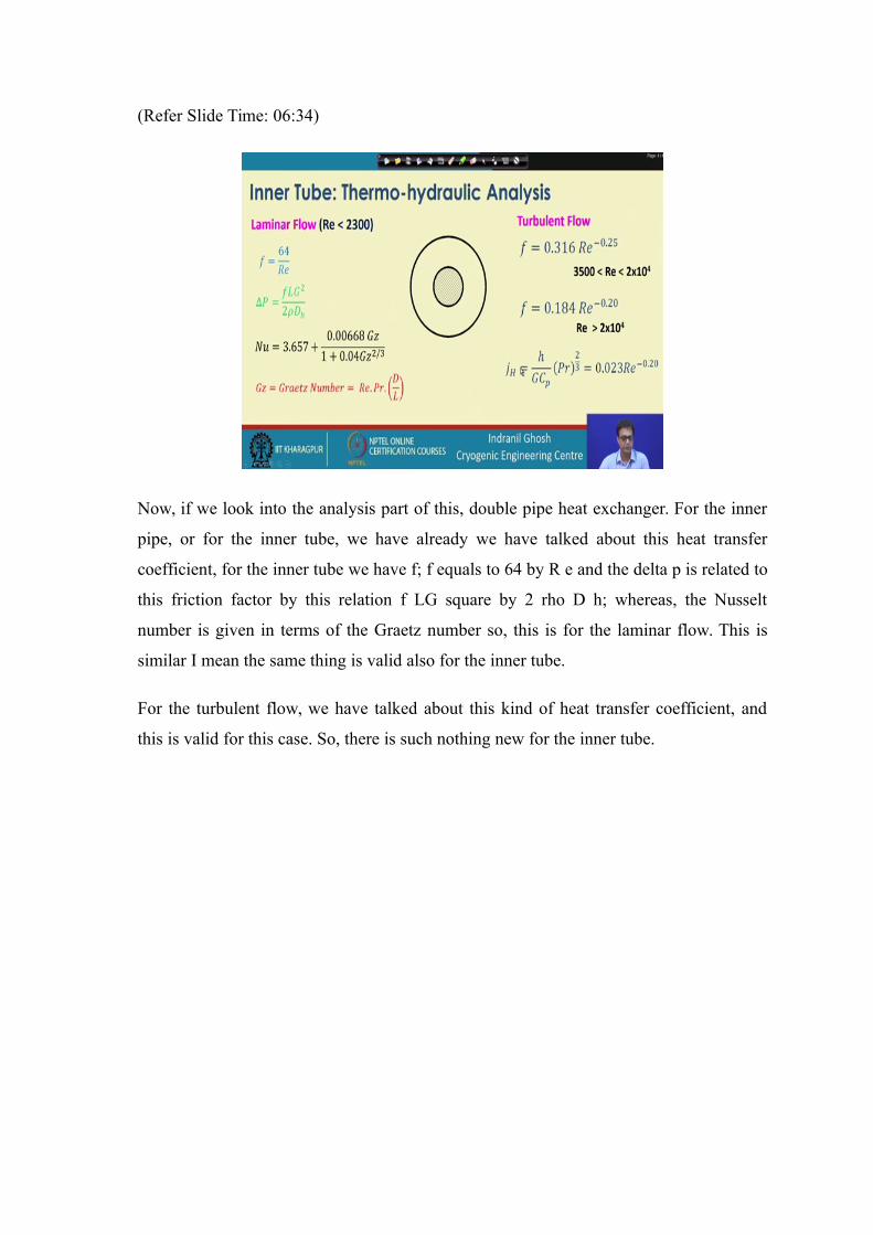
Now, if we look into the analysis part of this, double pipe heat exchanger. For the inner

pipe, or for the inner tube, we have already we have talked about this heat transfer

coefficient, for the inner tube we have f; f equals to 64 by R e and the delta p is related to

this friction factor by this relation f LG square by 2 rho D h; whereas, the Nusselt

number is given in terms of the Graetz number so, this is for the laminar flow. This is

similar I mean the same thing is valid also for the inner tube.

For the turbulent flow, we have talked about this kind of heat transfer coefficient, and

this is valid for this case. So, there is such nothing new for the inner tube.


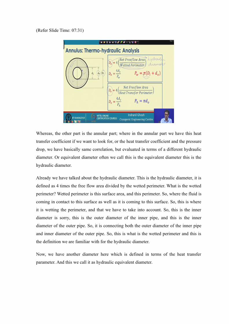
Whereas, the other part is the annular part; where in the annular part we have this heat

transfer coefficient if we want to look for, or the heat transfer coefficient and the pressure

drop, we have basically same correlation, but evaluated in terms of a different hydraulic

diameter. Or equivalent diameter often we call this is the equivalent diameter this is the

hydraulic diameter.

Already we have talked about the hydraulic diameter. This is the hydraulic diameter, it is

defined as 4 times the free flow area divided by the wetted perimeter. What is the wetted

perimeter? Wetted perimeter is this surface area, and this perimeter. So, where the fluid is

coming in contact to this surface as well as it is coming to this surface. So, this is where

it is wetting the perimeter, and that we have to take into account. So, this is the inner

diameter is sorry, this is the outer diameter of the inner pipe, and this is the inner

diameter of the outer pipe. So, it is connecting both the outer diameter of the inner pipe

and inner diameter of the outer pipe. So, this is what is the wetted perimeter and this is

the definition we are familiar with for the hydraulic diameter.

Now, we have another diameter here which is defined in terms of the heat transfer

parameter. And this we call it as hydraulic equivalent diameter.


This equivalent diameter, now what is the heat transfer parameter? The heat transfer

parameter, the heat transfer is occurring in terms of only through this area because we

have the inner fluid flowing through this tube and the fluid flowing at the annular space

another fluid. So, the heat transfer is taking place through this surface and that is related

to pi d 0.

So, d 0 is the external diameter of the inner tube and we define the equivalent diameter

by the 4 times the net free flow area, it remains the same this is the net free flow area and

this hatched part. So, this hatched part is basically the net free flow area, divided by the

heat transfer perimeter and that is how we will be getting the equivalent diameter.

So, this two terms will be coming otherwise the same correlations can be used for the

annular space, except that we have to use this hydraulic diameter or the equivalent

diameter for the appropriate calculation. So, we look into that how do we do that.


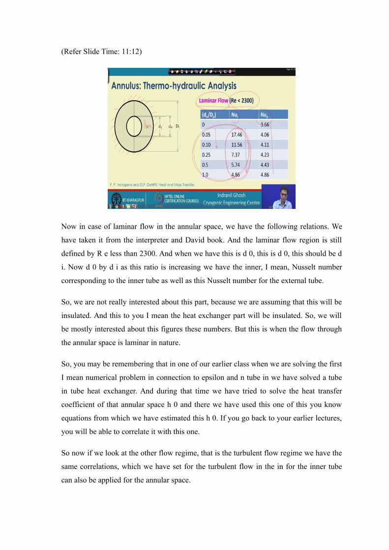
Now in case of laminar flow in the annular space, we have the following relations. We

have taken it from the interpreter and David book. And the laminar flow region is still

defined by R e less than 2300. And when we have this is d 0, this is d 0, this should be d

i. Now d 0 by d i as this ratio is increasing we have the inner, I mean, Nusselt number

corresponding to the inner tube as well as this Nusselt number for the external tube.

So, we are not really interested about this part, because we are assuming that this will be

insulated. And this to you I mean the heat exchanger part will be insulated. So, we will

be mostly interested about this figures these numbers. But this is when the flow through

the annular space is laminar in nature.

So, you may be remembering that in one of our earlier class when we are solving the first

I mean numerical problem in connection to epsilon and n tube in we have solved a tube

in tube heat exchanger. And during that time we have tried to solve the heat transfer

coefficient of that annular space h 0 and there we have used this one of this you know

equations from which we have estimated this h 0. If you go back to your earlier lectures,

you will be able to correlate it with this one.

So now if we look at the other flow regime, that is the turbulent flow regime we have the

same correlations, which we have set for the turbulent flow in the in for the inner tube

can also be applied for the annular space.


But this is another heat transfer correlation which is, you know, which can be used either

for the inner tube or for the annular space with the appropriate hydraulic diameter. And

here this is related to the friction factor given by this; 1.58 ln R e etcetera. So, we will

make use of these correlations while solving the numerical problem.


So, based on this analysis, now we will try to solve a numerical problem, where we find

that water with the flow rate of 500 kg per hour is heated up from 20 degree to 35 degree

centigrade by hot water at 140 degree centigrade. And there is 15-degree temperature

drop allowed with the water and we have 3.5 meter hairpin of 3 inch by 2 inch.

So, by saying this one we have specified the outer diameter and also we have specified

the inner diameter. Look we have been given, the inner diameter OD and ID both. So, it

is a counter flow double pipe heat exchanger with annuli and pipes, each connected in

series. So, this is important, and hot water flows through the inner tube. So now, we

know that we have double pipe exchanger with the inner one is having the hot water, and

outer one is having that cold water. So, this warm water with the warm water 140 degree

is the entry. And 15-degree temperature drop is allowable whereas, this cold water has to

be heated up from 20 degree to 35 degree.

Now, I assume that the pipe is made of carbon steel so that once we know what is the

material then we know the thermal conductivity of the material. And the heat exchanger

is insulated against the heat losses; that means this part of the exchanger is insulated. So,

there is no external heat. And we need to calculate the number of hairpins. So, with this

information let us try to solve this numerical problem.

So, first of all what we need to find out is the average temperature of the water.


So, here we have been told that, the hot water is entering at 140 degree Centigrade and

the other end of the fluid I mean when it is coming out it is only 15-degree temperature

drop is allowed. So, it should be 1 minus 15 degree. So, the other end temperature is also

known and we 125 degree C.

So, we take an average between 140 and 125 so, it is 132.5 degree centigrade. So, at this

average temperature, we are now suppose to find out the properties of water. So, if we

find out the properties of water, we will find the density to be 932.53 kg per meter cube.

Then we have thermal conductivity of the fluid as 0.687 watt per meter Kelvin. Then we

have Prandtl number as 1.28, and C p is equals to 4.268 kg joule per kg Kelvin. BO is

also known mu has been given as 0.207 into 10 to the power of minus 3 Pascal second.

So, these are the fluid properties or the properties of water evaluated at an average

temperature of 132.5 degree centigrade, and with this information we now suppose to

calculate the different heat transfer and etcetera. So, first of all we have been given or we

have been told about the mass flow rate of the cold water. We know the flow rate of we

know the temperature difference. So, what we have not been told is the flow rate of the

hot fluid. So, let us try to calculate the flow rate of the hot fluid and this can be done by

m h C ph delta T h is equals to m c dot both C pc into delta T c.

So, we have been told about this delta T h, we have been told about this delta T c. And

we know what are the cold fluid flow rate we know the C pc. And we can also find out

the delta T c. So, already we have all the properties known so, we can from there

calculate the m h dot and this will come out to be 1.36 kg per second. So, C p is taken as

of the cold water it has been taken as 4.179 joule per kg Kelvin. And we have also taken

this is at the bulk temperature of 27.5 degree C. This is an average temperature between

20 and 35.

So, we know that cold water is entering at 20 degree C, and it is leaving at 35 degree C.

So, 20 27.5 is the average temperature of the cold fluid. And at that temperature we have

evaluated the C pc. So, the C pc is also known in that equation we have used. And this is

how we know the hot fluid mass flow rate. So, if we know the hot fluid mass flow rate,

then we can try to calculate first of all the velocity and or we can also take the G, the

mass flow rate divided by the free flow area.


And then we can apply this relation G D h by mu to calculate the Reynolds number or

we can also try to find out the velocity by m dot by rho AC. So, here if it is for the hot

fluid it will be rho h AC, and you can find out it to be say 0.673 meter per second.

So, once we know the velocity, then we can calculate the Reynolds number as rho u d by

m h dot so, this will come out. So, I am sorry, this will be rho v d by mu. And this will

come out to be 159343. So, this is just nothing but the Reynolds number of the hot fluid,

the hot fluid is flowing through the inner tube. So, it is flowing through the inner tube.

We know the Reynolds number; it is much more than 2300 and obviously, we can

understand that this is a turbulent flow. So, we have to use the turbulent Reynolds

number, I mean turbulence correlations.


And as we have said that we will be using the Nusselt number at the bulk temperature as

I have shown it, this is f by 2 into R e to the power this is P r that bulk divided by 1 plus

8.7 into f by 2 whole to the power half. And P r b minus evaluated at the bulk mean

temperature divided minus 1.

And this f is related to 1.58 into ln of R e minus 3.28 this whole square. And accordingly

if you use we know first of all we have already calculated the R e. So, you would be able

to calculate the f. So, f will come out to be 4.085 into 10 to the power minus 3. And this

value will be substituted to that earlier equation, where we know if we know R e, we

know P r and we will be able to find out this Nusselt number. So, this Nusselt number N

ub is equals to 375.3, if you evaluate it you will be able to find it out.

So, this is just nothing but h i D of the hydraulic diameter h d by k, k of the fluid. So,

accordingly we can find out the heat transfer coefficient of the inner tube hydraulic

diameter already we know, that is the inner tube. So, we can find out the h i, and this will

come out to be 4911 point this one watt per meter square Kelvin.

So, to determine now the heat transfer coefficient of the annular part, what we need to do

is that. We need to find out the Reynolds number, and in the annular space, then we have

to use the appropriate correlation we can again use this correlation, but we may have to

depending on whether we are calculating the friction factor or the what is called the

friction factor or the Nusselt number or the heat transfer we have to use either hydraulic

diameter or the equivalent diameter.


So let us first try to find out the fluid properties as we have said that for the cold fluid.

We know that the average temperature is for the cold fluid the average temperature is

27.5 degree centigrade. And entered temperature we have the row equals to 996.4 kg per

meter cube. And we also have k is equals to 0.609 watt per meter Kelvin. Then we have

C p is equals to 4.179 joule per kg Kelvin. Then we have P r equals to 5.77. So, as the

temperature has reduced, now we have the higher value of the Prandtl number, and we

have the mu equals to 8.41 into 10 to the power minus 6 Pascal second.

So, we have these values to evaluate the fluid properties or calculate the different

parameters for the annuli space. First of all, we need to find out the velocity. How do we

will find out the velocity? So, we calculate we know the mass flow rate and then we find

out the A C and rho. What is that A C? The A C is just nothing but there is this free flow

area this is the cross sectional area. And we can find out this 1 by pi by 4. This is the

inner diameter of the outer one, and this is the outer diameter d 0 of the inner tube. So,

we will use those 2 parameters we know already.

So, D i square minus d 0 square. So, this is the free flow area and we know the density of

the cold liquid. So, we will be able to find out the velocity of the hot fluid. This will

come out to be 0.729 meter per second. You can try, and the hydraulic diameter.


The hydraulic diameter can be calculated as how is the hydraulic diameter 4 times that

free flow area, does just now we have calculated and that P w which is nothing but pi d 0

plus D i. And we have 4 times 4 by pi D square D i square minus d 0 square by 4, this is

pi.

So, from here you would be able to find out the hydraulic diameter, and this hydraulic

diameter will come out to be 0.0176 meter. Now the Reynolds number so, we know the

hydraulic diameter, we know the u m rho v d hydraulic diameter for this one and by the

mu.

So, this comes out to be 1500 0 to 1. So, this is also more than 2300 so, we have

turbulent flow region.


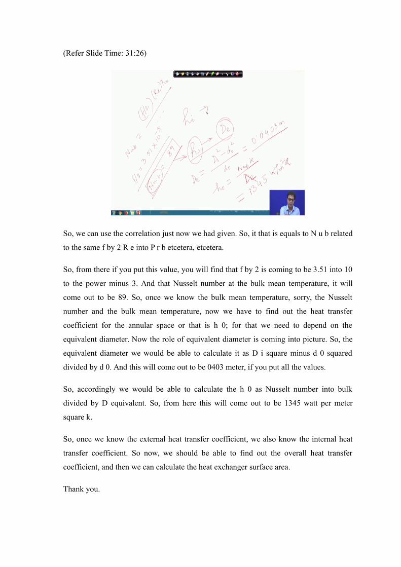
So, we can use the correlation just now we had given. So, it that is equals to N u b related

to the same f by 2 R e into P r b etcetera, etcetera.

So, from there if you put this value, you will find that f by 2 is coming to be 3.51 into 10

to the power minus 3. And that Nusselt number at the bulk mean temperature, it will

come out to be 89. So, once we know the bulk mean temperature, sorry, the Nusselt

number and the bulk mean temperature, now we have to find out the heat transfer

coefficient for the annular space or that is h 0; for that we need to depend on the

equivalent diameter. Now the role of equivalent diameter is coming into picture. So, the

equivalent diameter we would be able to calculate it as D i square minus d 0 squared

divided by d 0. And this will come out to be 0403 meter, if you put all the values.

So, accordingly we would be able to calculate the h 0 as Nusselt number into bulk

divided by D equivalent. So, from here this will come out to be 1345 watt per meter

square k.

So, once we know the external heat transfer coefficient, we also know the internal heat

transfer coefficient. So now, we should be able to find out the overall heat transfer

coefficient, and then we can calculate the heat exchanger surface area.

Thank you.

Heat Exchangers: Fundamentals and Design Analysis Prof ... · Cryogenic Engineering Center Indian...

Documents

Transcript of Heat Exchangers: Fundamentals and Design Analysis Prof ... · Cryogenic Engineering Center Indian...