HEAT AND MASS TRANSFER DURING COOKING OF

CHICKPEA – MEASUREMENTS AND

COMPUTATIONAL SIMULATION

A Thesis Submitted to the

College of Graduate Studies and Research

In Partial Fulfillment of the Requirements

For the Degree of Master of Science

In the Department of Agricultural and Bioresource Engineering

University of Saskatchewan

Saskatoon, Saskatchewan

By

Nalaini D. Sabapathy

© Copyright Nalaini D. Sabapathy, March 2005. All rights reserved.

i

PERMISSION TO USE

In presenting this thesis in partial fulfillment of the requirements for a

Postgraduate degree from the University of Saskatchewan, I agree that the Libraries of

this University may make it freely available to inspection. I further agree permission for

copying of this thesis in any manner, in whole or part, for scholarly purposes may be

granted by the professor or professors who supervised my thesis work, or in their

absence, by the Head of the Department or the Dean of the College in which my thesis

work was done. It is understood that any copying or publication or use of this thesis or

parts thereof for financial gain shall not be allowed without my written permission. It is

also understood that due recognition shall be given to me and to the University of

Saskatchewan in any scholarly use which may be made of any material in my thesis.

Requests for permission to copy or to make other use of material in this thesis in

whole or in part should be addressed to:

Head, Department of Agricultural and Bioresource Engineering

University of Saskatchewan

Saskatoon, Saskatchewan

S7N 5A9

CANADA

ii

ABSTRACT

Chickpea is a food legume crop grown in tropical, sub-tropical and temperate

regions. World chickpea production is roughly three times that of lentils. Among pulse

crops marketed as human food, world chickpea consumption is second only to dry beans.

Turkey, Australia, Syria, Mexico, Argentina and Canada are major chickpea exporters.

There are two types of chickpea, namely, the kabuli and the desi. The kabuli type

is grown in temperate regions while the desi type chickpea is grown in the semi-arid

tropics. Chickpea is valued for its nutritive seeds with high protein and starch content.

They are eaten fresh as green vegetables, parched, fried, roasted, and boiled, as snack

food, dessert and condiments. The seeds are ground and the flour can be used in soup,

dhal and bread. Cooked chickpea is mostly preferred by consumers, especially the kabuli

type.

In this thesis, the heat and moisture transfer behavior of kabuli chickpea when

subjected to cooking at different temperatures was investigated. The thermo-physical

properties of chickpea were studied to develop a model to simulate the temperature

distribution and moisture absorption in a chickpea seed when cooked in water.

The thermo-physical properties determined experimentally were thermal

conductivity, specific heat, moisture diffusivity, particle density and moisture content.

Thermal diffusivity was calculated using the experimental values of thermal conductivity,

specific heat and density. The water absorption in chickpea was determined when the

seeds were soaked at different temperatures. It was observed that as the temperature of

the soaking medium was increased, the rate of moisture absorption also increased.

Soaking was done to enhance the gelatinization process during cooking. Cooking

iii

experiments were conducted for boiling temperatures ranging from 70 to 98°C for both

soaked and unsoaked seeds. It resulted in the soaked seeds being cooked within 40-50

min, whereas the unsoaked seeds took around 250-300 min to cook. The amount of

soluble solids lost during the cooking process is also reported which enables to predict

the optimum soaking and cooking temperature.

Using linear regression simple models for dependency of thermal conductivity,

specific heat, thermal diffusivity and density on temperature and moisture content were

developed. The rate of moisture transfer and the center temperature in the seed during

cooking was determined experimentally and also simulated with the constant thermal

properties found experimentally. The closeness of the simulated and experimental results

was proved by appropriate statistical analysis.

Based on the results obtained, it can be understood that soaking the chickpea

seeds at temperatures ranging from 25 to 40°C for 8 h and cooking it at higher

temperatures ranging from 90 to 100°C will improve the quality of the cooked seed with

minimum mass loss. This optimum condition saves both energy and time.

iv

ACKNOWLEDGEMENTS

I would like to express my gratitude to all those who gave me the possibility to

complete this thesis.

I am deeply indebted to my supervisor Prof. Dr. Lope G. Tabil Jr. whose help,

stimulating suggestions, patience and encouragement helped me in all the time of

research and writing of this thesis.

I would also like to thank my graduate committee members Dr H. Guo and Dr

Oon-Doo Baik, for following the progress and giving valuable suggestions throughout

my research program.

I acknowledge the financial support from the National Sciences and Engineering

Research council of Canada (NSERC), Canada Saskatchewan Agri-Food Innovation

Fund (AFIF) and the Agriculture Development Fund of Saskatchewan Agriculture, Food

and Revitalization (ADF).

I would also like to thank the Department of Electrical Engineering, University of

Saskatchewan for providing the facilities and equipment for the specific heat

measurement.

My colleagues from the Department of Agricultural and Bioresource Engineering,

Saskatoon, Saskatchewan, Canada, supported me in my research work. I want to thank

them for all their help, support, interest and valuable hints. Especially I am obliged of the

assistance extended by Mr. Bill Crerar, research engineer and Mr. Wayne Morley,

electronics technologist.

v

DEDICATION

I dedicate this thesis to my beloved family.

vi

TABLE OF CONTENTS

PERMISSION TO USE……………………………………………………………. i

ABSTRACT………………………………………………………………………... ii

ACKNOWLEDGEMENTS………………………………………………………... iv

DEDICATION……………………………………………………………………… v

TABLE OF CONTENTS…………………………………………………………... vi

LIST OF FIGURES………………………………………………………………... ix

LIST OF TABLES…………………………………………………………………. xii

1. INTRODUCTION…………………………………………………………….. 1

2. OBJECTIVES…………………………………………………………………. 4

3. LITERATURE REVIEW……………………………………………………… 5 3.1 Thermo-physical Properties……………………………………………….. 5 3.1.1 Physical properties………………………………………………... 5 3.1.2 Thermal properties………………………………………………... 9 3.1.3 Soaking and water absorption……………………………………. 14 3.1.4 Cooking characteristics of chickpea……………………………… 16 3.1.4.1 Effect of cooking on chickpeas…………………………. 17 3.1.4.2 Conventional methods of cooking……………………… 20 3.1.4.3 Modern methods of cooking……………………………. 22 3.2 Heat and Mass Transfer…………………………………………………… 26 3.3 Mathematical Modeling…………………………………………………... 28

3.4 Summary……………...…………………………………………………... 30

4. MATERIALS AND METHODS……………………………………………… 31 4.1 Material…………………………………………………………………... 31 4.2 Moisture Content Determination………………………………………… 31 4.3 Density Measurement……………………………………………………. 32 4.4 Thermal Conductivity……………………………………………………. 35 4.4.1 Thermal conductivity measurement using the assembled probe… 35 4.4.1.1 Probe construction……………………………………. 36 4.4.1.2 Measurement technique for assembled probe method.. 37 4.4.1.3 Thermal conductivity of distilled water……………… 40 4.4.1.4 Thermal conductivity measurement of chickpea……... 41 4.4.2 Thermal conductivity measurement using the KD2 Thermal 43

vii

properties analyzer…………………………………………….. 4.5 Specific Heat…………………………………………………………… 44 4.5.1 Assembled calorimeter………………………………………... 44 4.5.1.1 Apparatus…………………………………………….. 45 4.5.1.2 Heat capacity measurement of calorimeter…………... 48 4.5.1.3 Specific heat measurement of chickpea using the

assembled calorimeter ………………………………………... 50

4.5.2 Differential scanning calorimetry……………………………... 52 4.5.2.1 Apparatus……………………………………………... 52 4.5.2.2 Sample preparation for measurements……………….. 53 4.5.2.3 Specific heat measurement by the DSC……………… 53 4.6 Thermal Diffusivity…………………………………………………….. 56 4.7 Water Absorption During Soaking……………………………………... 57 4.8 Moisture Diffusivity Measurement During Cooking…………………... 58 4.8.1 Measurement of moisture diffusivity…………………………. 58 4.9 Temperature Measurement in the Center of Chickpea…………………. 59 4.9.1 Sample preparation……………………………………………. 60 4.9.2 Temperature measurement……………………………………. 60 4.10 Solid Loss During Cooking…………………………………………….. 61 4.10.1 Solid loss measurement……………………………………….. 61

5. MODELING AND SIMULATION…………………………………………… 63 5.1 Assumptions in Modeling……………………………………………… 64 5.2 Governing Equations and Boundary Conditions for Heat and Mass

Transfer…………………………………………………………………. 65

5.2.1 Heat and mass transfer………………………………………… 65 5.2.2 Initial and boundary conditions……………………………….. 67 5.3 Non-dimensional Analysis……………………………………………... 69 5.4 Solution Method………………………………………………………... 71 5.4.1 Development of finite difference equations…………………... 71 5.4.2 Discretization of the equations………………………………... 72 5.5 Properties Used in Model Calculations………………………………… 75 5.5.1 Surface heat transfer coefficient (ht)………………………….. 75 5.5.2 Calculation of convective heat transfer coefficient…………… 75 5.5.3 Diffusion coefficient (Dm)…………………………………….. 77 6. RESULTS AND DISCUSSION……………………………………………….. 78 6.1 Moisture Content……………………………………………………….. 78 6.2 Density………………………………………………………………….. 79 6.3 Thermal Conductivity…………………………………………………... 81 6.4 Specific Heat…………………………………………………………… 85 6.4.1 Assembled calorimeter method……………………………….. 86 6.4.2 DSC method………………………………………………….. 88 6.5 Thermal Diffusivity……………………………………………………. 90 6.6 Moisture Absorption of Chickpea……………………………………… 93 6.7 Cooking Time of Chickpea…………………………………………….. 95

viii

6.7.1 Temperature of the center of chickpea during cooking……….. 98 6.7.2 Moisture diffusivity…………………………………………… 99 6.8 Mass Loss………………………………………………………………. 100 6.9 Simulation Results ……………………………………………………... 101 6.9.1 Transport properties used in modeling………………………... 102 6.9.2 Simulated and experimental temperature and moisture

histories………………………………………………………... 102

7. SUMMARY AND CONCLUSION…………………………………………… 106

8. RECOMMENDATIONS………………………………………………………. 108

REFERENCES……………………………………………………………………… 110

APPENDICES………………………………………………………………………. 120

APPENDIX A Specific Heat Measurement by DSC…………………………………………… 121

APPENDIX B Simulation Programs Used to Predict the Heat and Mass Transfer During

Cooking of Chickpea…………………………………………………………… 124

APPENDIX C Simulated Temperature History…...…………………………………………… 128

APPENDIX D Deviations of the Simulated from the Experimental Moisture and

Temperature Profiles……………...…………………………………………… 141

APPENDIX E Experimental and Simulated Results…………………………………….…..… 148

APPENDIX F Experimental Values Shown in Replicates…...………………………………… 151

ix

LIST OF FIGURES

Figure 4.1 Multipycnometer used for measuring particle density…………………. 33

Figure 4.2 Schematic diagram of gas multipycnometer…………………………… 34

Figure 4.3 Assembled probe for thermal conductivity measurements…………….. 37

Figure 4.4 Schematic diagram of the thermal conductivity measurement………… 38

Figure 4.5 Thermal conductivity probe with chickpea seed sample………………. 42

Figure 4.6 Measurement of thermal conductivity of chickpea…………………….. 42

Figure 4.7 Measurement of thermal conductivity using the KD2 thermal properties analyzer……………………………………………………... 44

Figure 4.8 Assembled calorimeters A and B………………………………………. 45

Figure 4.9 Dewar flask with thermocouples attached……………………………... 46

Figure 4.10 Diagram of the calorimeter used for measuring specific heat of chickpea………………………………………………………………… 47

Figure 4.11 Packing gland used to insert thermocouples into the Nylon Polyethylene bag……………………………………………………….. 48

Figure 4.12 Experimental set up during heat capacity measurement……………….. 49

Figure 4.13 Sample in plastic pouch with thermocouples…………………………... 50

Figure 4.14 Pouring water from calorimeter B to calorimeter A during specific heat measurement……………..………………………………. 51

Figure 4.15 Differential Scanning Calorimetry instrument…………………………. 54

Figure 4.16 DSC Sample holder…………………………………………………….. 54

Figure 4.17 Schematic of the DSC for specific heat measurement…………………. 55

Figure 4.18 Ground samples and samples sealed in pans…………………………… 55

Figure 4.19 Soaked chickpea………………………………………………………... 62

Figure 4.20 Solid loss during soaking………………………………………………. 62

Figure 5.1 Direction of heat and mass flow during cooking of chickpea………….. 64

Figure 5.2 Position of nodes in the chickpea………………………………………. 71

Figure 5.3 Aluminum sphere and chickpea seed during measurement of heat transfer coefficient……………………………………………………… 76

Figure 6.1 Seed density as a function of seed moisture content…………………… 80

Figure 6.2 Typical experimental temperature history of distilled water at an initial temperature of 25ºC; T= temperature at any time (ºC) and To = initial temperature (°C)……………… ………………………. 82

x

Figure 6.3 Typical temperature history curve for chickpea during measurement of thermal conductivity……..…………………………… 82

Figure 6.4 Thermal conductivity of chickpea as a function of moisture content and temperature………………………………………………………… 84

Figure 6.5 Time-temperature data during heat capacity measurement of calorimeter……………………………………………………………… 86

Figure 6.6 Typical time-temperature curve for specific heat measurement of sample using assembled calorimeter method…………………………... 87

Figure 6.7 Specific heat values obtained from the DSC…………………………… 90

Figure 6.8 Thermal diffusivity values obtained by assembled calorimeter method…………………………………………………………………. 91

Figure 6.9 Thermal diffusivity values obtained by DSC method………………….. 92

Figure 6.10 Moisture absorption of chickpea during soaking in water……………... 93

Figure 6.11 Cooking of soaked and unsoaked chickpea at 98°C…………………… 97

Figure 6.12 Center temperature of unsoaked chickpea during cooking at different temperatures………………………………………………….. 98

Figure 6.13 Center temperature of soaked chickpea during cooking at different temperatures……………………………………………………………. 99

Figure 6.14 Experimental and simulated center temperature during cooking of unsoaked chickpea……………………………………………………… 103

Figure 6.15 Experimental and simulated center temperature during cooking of soaked chickpea………………………………………………………… 103

Figure 6.16 Experimental and simulated moisture ratio during cooking of unsoaked chickpea………………………………………………….. 104

Figure 6.17 Experimental and simulated moisture ratio during cooking of soaked chickpea….………………………………………… 105

xi

LIST OF TABLES

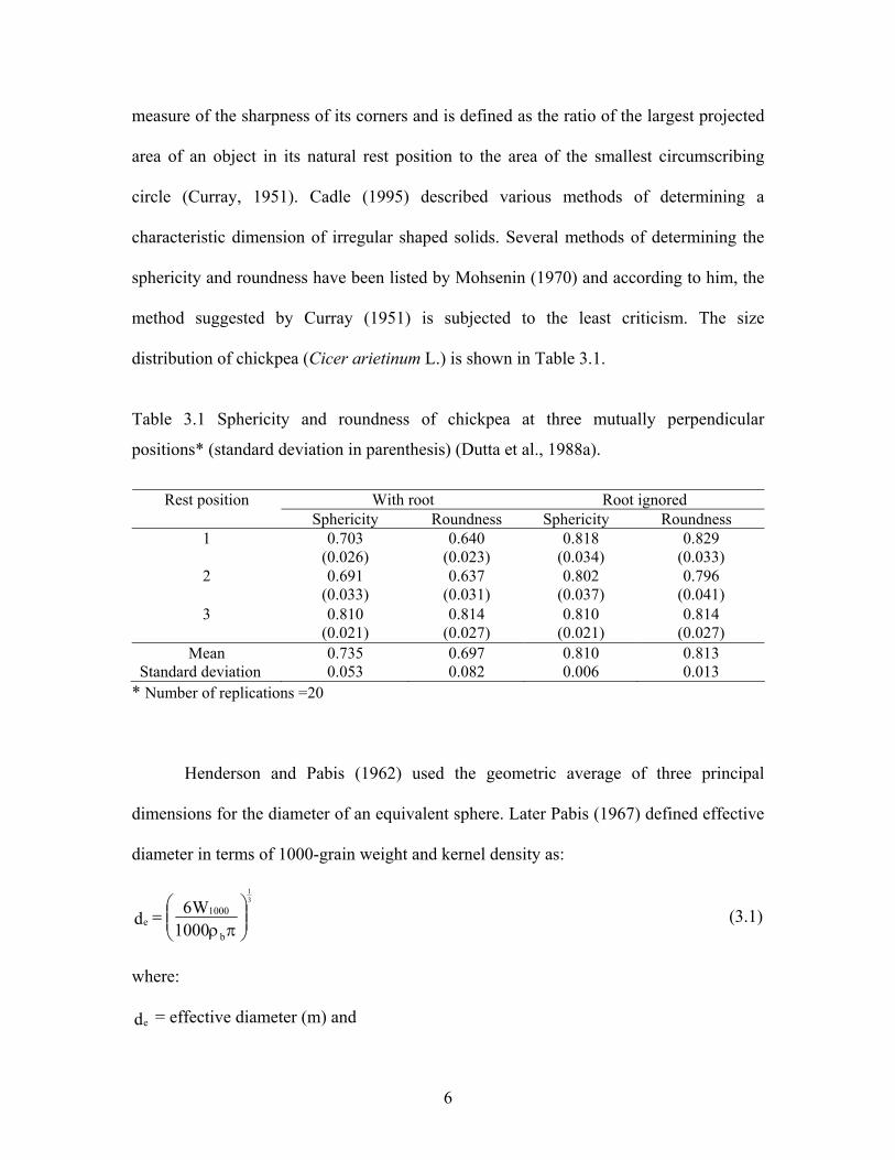
Table 3.1 Sphericity and roundness of chickpea at three mutually perpendicular positions…………………………………………….. 6

Table 3.2 Physical attributes of chickpea seed at 5.2 % dry basis…………… 7

Table 3.3 Physicochemical characteristics of treated chickpea………………. 18

Table 3.4 Average physical dimension of legume seeds……………………… 24

Table 6.1 Moisture content of chickpea seed samples used in experiments….. 78

Table 6.2 Particle density of chickpea as a function of moisture content…….. 80

Table 6.3 Determination of thermal conductivity using the assembled probe... 83

Table 6.4 Specific heat values for chickpea by assembled calorimeter method……………………………………………………………… 87

Table 6.5 Cooking time and moisture content of chickpea at varying temperatures………………………………………………………... 96

Table 6.6 Diffusion coefficient values………………………………………... 99

Table 6.7 Determination of solids loss during soaking of chickpea………….. 101

1

1. INTRODUCTION

Food legumes have been well recognized as valuable source of dietary proteins in

many parts of the world. A major portion of the world population relies on legumes as

staple food particularly in combination with cereals.

Chickpea (Cicer arietinum L.) is a cool season food legume crop grown in more

than 45 countries of the world. It is the third most commonly consumed legume in the

world (Singh et al., 1991). It is one of the staple foods in the Middle Eastern countries,

and half of the world’s annual chickpea production comes from Syria and Turkey (Singh

et al., 1990).

Chickpea is commonly utilized in whole or paste form as a main or side dish after

cooking (Amr and Yaseen, 1994) and in whole form as a snack food after roasting

(Koksel et al., 1998). Different heat treatment methods are used to prepare chickpea

namely, conventional methods like cooking in water, pressure cooking, roasting, puffing

and modern methods like microwave and infrared heating. Chickpea cooked in water is

mostly preferred by consumers since it produces a tender edible product with aroma.

Cooking also inactivates antinutritional factors present in the grain. There are two main

types of chickpea namely, the kabuli and the desi, but the most preferred type for cooking

is the kabuli. Kabuli seeds are large in size, salmon white in color and contain high levels

of carbohydrates and proteins.

Legume grains require a relatively long cooking time ranging from 1 to 4 h (FAO,

1979). Each cooking process involves simultaneous heat and mass transport phenomena,

physical and chemical reactions such as starch gelatinization and protein denaturation.

2

Boiling is performed at temperatures below or around 100˚C in either water or soups

(Skjoldebrand, 1984). Absorption of water by the chickpea during soaking and boiling at

relatively low temperatures below 100˚C promotes a soft and moist product texture, with

minimal mass loss. Cooking time of legumes primarily depends on the softness of the

cooked seeds. In order to find the optimum cooking time, information on the thermal

properties and the heat and mass transfer characteristics should be known.

Previous studies were done on different methods of cooking chickpea based on

its cooking time and nutritional factors. However, heat and mass transfer characteristics

of chickpea has so far not been studied. The relationship between cooking time and some

physical characteristics in chickpea was studied by Williams and co-workers (1983),

however, not much work was done on the thermal properties of chickpea. Traditionally

prior to cooking, chickpea grains should be soaked for a period of approximately 10 to 12

h. The size, composition and structure of legume seed, water absorption and rate of heat

transfer, has a large influence on the cooking time and quality of the cooked seed.

Therefore, any preliminary processing that causes changes in the characteristics of the

seed affects the cooking properties. In order to maintain the appearance, texture, structure

of the seed and prevent them from splitting and damaging the seed when subjected to

cooking in water, suitable models for heat and moisture transfer of the seed should be

developed. Based on the results obtained, optimum soaking and cooking time can be

determined. In this study, emphasis has been given on the thermo-physical properties and

the heat and mass transfer characteristics during cooking.

Mathematical modeling and simulation of the cooking process play an important

role in designing and optimizing the cooking process. The current research involves

3

modeling, simulating and validating the heat and moisture transfer phenomena within the

chickpea seed during cooking process to predict the heat and the moisture transfer within

the seed. Mathematical equations were developed of the time-dependent heat and

moisture transfer into the seed.

The objectives of this thesis are given in chapter 2 and the literature review is

presented in chapter 3. The materials and methods are explained in chapter 4. Chapter 4

has a detailed description on the experiments that were conducted. Mathematical

modeling and simulation information are presented in chapter 5. In chapters 6 and 7, the

results are analyzed and discussed and the summary and conclusions is presented.

Recommendations are given in chapter 8. Results of the simulation on temperature

distribution and moisture diffusion are given in the appendices.

4

2. OBJECTIVES

The principal objective of this thesis is to model and simulate heat and mass

transfer during cooking of chickpea seed with water and to predict the optimum cooking

time. The specific objectives are:

1) to develop heat and mass transfer equations during cooking of chickpea grain ;

2) to study the thermo-physical properties of the chickpea grain ;

3) to experimentally measure the temperature distribution and moisture absorption of

the grain during cooking ; and

4) to predict the temperature distribution and moisture absorption during cooking of

chickpea grain and validate the model predicted results with the experimental

data.

5

3. LITERATURE REVIEW

This chapter consists of two sections. The first section is a review of the thermo-

physical properties, soaking and water absorption, and the cooking characteristics of the

chickpea grain. The second section is a review of the heat and mass transfer theories and

the relevant numerical techniques to solve the equation systems. Application of the heat

and mass transfer model in the food system is also reviewed in the second section.

3.1 Thermo-physical Properties

In order to conduct effective process modeling and simulation in each application

at every stage, there is a need for consistent thermo-physical property information. Hence

a review of thermo-physical properties that have been reported in literature is addressed

in this section.

3.1.1 Physical properties

Some of the physical properties include 1000-grain weight, sphericity, roundness,

size, volume, shape, surface area, bulk density, kernel density, porosity, static coefficient

of friction against different materials and angle of repose. Limited research has been

conducted on the physical properties of chickpea. Some engineering properties of

chickpea seeds, such as density, terminal velocity and coefficient of drag, were reported

by Kural and Carman (1997).

Sphericity is defined as the ratio of the surface area of a sphere, which has the

same volume as that of the solid, to the surface area of the solid. Roundness of a solid is a

6

measure of the sharpness of its corners and is defined as the ratio of the largest projected

area of an object in its natural rest position to the area of the smallest circumscribing

circle (Curray, 1951). Cadle (1995) described various methods of determining a

characteristic dimension of irregular shaped solids. Several methods of determining the

sphericity and roundness have been listed by Mohsenin (1970) and according to him, the

method suggested by Curray (1951) is subjected to the least criticism. The size

distribution of chickpea (Cicer arietinum L.) is shown in Table 3.1.

Table 3.1 Sphericity and roundness of chickpea at three mutually perpendicular

positions* (standard deviation in parenthesis) (Dutta et al., 1988a).

With root Root ignored Rest position

Sphericity Roundness Sphericity Roundness 1 0.703

(0.026) 0.640

(0.023) 0.818

(0.034) 0.829

(0.033) 2 0.691

(0.033) 0.637

(0.031) 0.802

(0.037) 0.796

(0.041) 3 0.810

(0.021) 0.814

(0.027) 0.810

(0.021) 0.814

(0.027) Mean

Standard deviation 0.735 0.053

0.697 0.082

0.810 0.006

0.813 0.013

* Number of replications =20

Henderson and Pabis (1962) used the geometric average of three principal

dimensions for the diameter of an equivalent sphere. Later Pabis (1967) defined effective

diameter in terms of 1000-grain weight and kernel density as:

31

b

1000e 1000

W6d

πρ

= (3.1)

where:

de = effective diameter (m) and

7

ρb = bulk density of the grain (kg/m3).

The geometric mean diameter dp of the seed can be calculated by using the following

relationship (Mohsenin, 1970):

31

)LWT(dp = (3.2)

where:

L = length (mm),

W = width (mm) and

T = thickness (mm).

Table 3.2 shows the dimensions of the seed at 5.2% moisture content reported by Konak

et al. (2002), where about 70% of the seeds have a length ranging from 8.50 to 9.50 mm

and about 85 to 89% width and thickness ranging from 7.00 to 8.00 mm.

Table 3.2 Physical attributes of chickpea seed at 5.2% dry basis (Konak et al., 2002).

Attribute Mean ± SD Length, mm 9.342 ± 0.118 Thickness, mm 7.752 ± 0.087 Width, mm 7.722 ± 0.103 Geometric mean diameter, mm 8.358 ± 0.089 Sphericity, % 87.589 ± 0.474 Mass, g 0.324 ± 0.003 Volume, cm3 0.238 ± 0.027

SD = Standard deviation

Bulk density is the ratio of the mass of a sample of food grain to its total volume.

It is a moisture dependent property and is found by filling a standard container with grain

by pouring it from a certain height, striking off the top level and then weighing the

contents. Bulk density of the seeds varied according to different moisture levels from

741.4 to 800 kg/m3 and indicated a decrease in bulk density with an increase in moisture

8

content (Konak et al., 2002). The inverse linear relationship of bulk density with moisture

content was also reported for pigeon pea (Shepherd and Bhardwaj, 1986) and soybean

(Deshpande et al., 1993).

The kernel density of a seed is defined as the ratio of the mass of a sample of a

seed to the solid volume occupied by the sample (Deshpande et al., 1993). Kernel density

of chickpea at different moisture levels varied from 1428 to 1368 kg/m3. As moisture

content increased, the kernel density of chickpea seed decreased (Konak et al., 2002).

Porosity is the property of the grain, which depends on its bulk and kernel

densities. The values of porosity of various grains as measured with the help of an air

comparison pycnometer which measures the volume by using high pressure air was

reported by Thompson and Isaacs (1967). The air comparison pyconometer displaces

high pressure air which is measured with the help of a manometer and the displaced

volume is measured. The porosity, ε of bulk seed is computed from the values of kernel

density in the relationship given by Mohsenin (1970) using the following equation:

100ρρ-ρ

=εk

bk (3.3)

where:

ρb = bulk density (kg/m3), and

ρk = kernel density (kg/m3).

Porosity of chickpea seed increases with an increase in moisture content from 5.2

to 16.5% d.b. (Konak et al., 2002). Carman (1996) reported a similar increase in porosity

from a moisture content of 27.5 to 32.2% (d.b.) for lentil.

Projected area of chickpea seed increased by about 22.4%, when the moisture

9

content of seed increased from 5.2 to 16.5% d.b. Similar trends were observed in other

seeds (Mohsenin, 1970; Sitkei, 1986).

The angle of repose of the chickpea seed increased from 24.5 to 27.9ºC in the

moisture range of 5.2-16.5% d.b. The value of angle of repose for chickpea seed was

considerably less than those reported for pumpkin, pigeon pea and fababean seeds (Fraser

et al., 1978; Shepherd and Bhardwaj 1986). This may be due to the higher sphericity of

chickpea seeds allowing them to slide and roll on each other (Konak et al., 2002).

Rupture strength is usually dependent on the moisture content. The highest

rupture force obtained was 210 N at a moisture content of 5.2% d.b (Konak et al., 2002).

Generally the seeds became more sensitive to cracking at high moisture content; hence,

they required less force to rupture.

3.1.2 Thermal properties

Thermal properties include specific heat, thermal conductivity and thermal

diffusivity. Specific heat is the quantity of the heat that is gained or lost by a unit mass of

product to accomplish a unit change in temperature, without a change in state. It can be

calculated as follows:

)T∆(mQ

=cp (3.4)

where:

Q = heat gained or lost (kJ),

m = mass (kg),

∆T = temperature change in the material (K), and

cp = specific heat (kJ/ kgK).

10

Specific heat is an essential part of the thermal analysis of food processing or of the

equipment used in heating or cooling of foods. A number of models express specific heat

as a function of water content, as water is a major component of many foods. Siebel

(1892) proposed that the specific heat of food materials such as eggs, meats, fruits and

vegetables can be taken as equal to the sum of the specific heat of water and solid matter.

One of the earliest models to calculate specific heat was proposed by Siebel (1892) as:

X349.3+837.0=c wp (3.5)

where:

Xw = water content expressed as a fraction.

The influence of product components was expressed in an empirical equation proposed

by Charm (1978) as:

X187.4+X256.1+X093.2=c wsfp (3.6)

where:

X = mass fraction, and

subscripts:

f = fat, s = nonfat solids, and w = water.

Other equations of similar form as Equation 3.5 have been summarized by Sweat

(1986). Choi and Okos (1983) gave a more generalized equation for specific heat which

takes into account the composition of food:

X908.0X547.1X928.1X711.1X180.4c acfpwp ++++= (3.7)

where:

X = mass or weight fraction of each component.

The subscripts denote the following components:

11

w = water, p = protein, f = fat, c = carbohydrate and, a = ash.

Although specific heat varies with temperature, for ranges near room temperature,

these changes are relatively minor. They are usually neglected in engineering

calculations. Sweat (1986) gave several equations for specific heat which include

temperature dependency.

Specific heat measurements can be done by the method of mixture, comparison

method, adiabatic method and differential scanning calorimetry (DSC). However in the

case of food materials, there are some problems due to direct mixing. The density of the

heat transfer medium should be lower than the food sample so that it will sink more

readily. Hwang and Hayakawa (1979) developed a calorimeter for measuring specific

heat of food materials by avoiding direct contact between food and heat exchange

medium in the calorimeter. The DSC is well-suited for determining the effect of

temperature on specific heat of food samples because it is easy to scan a wide range of

temperatures (Rao and Rizvi, 1995). The dynamic feature of DSC allows the

determination of specific heat as a function of temperature (Tang et al., 1991). McMillin

(1969) and Koch (1969) employed DSC to determine the specific heat of wood and dry

tree bark, respectively. Using DSC, Murata et al. (1987) determined the specific heat of

eight cereal grains over a temperature range of 10 to 70°C and a moisture content range

of 0 to 35% w.b. Tang et al. (1991) determined the specific heat capacity of lentil seeds

by DSC and reported that specific heat increased quadratically with moisture content over

the range from 2.1 to 25.8% w.b. and linearly with temperature varying from 10 to 80°C.

The use of DSC for measuring the heat capacity of chickpea was not reported.

The thermal conductivity of a food material is an important property used in

12

calculations involving rate of heat transfer. In quantitative terms, this property gives the

amount of heat that will be conducted per unit time through a unit thickness of the

material, if a unit temperature gradient exists across that thickness. Hooper and Lepper

(1950) determined thermal conductivity using the following equation:

∆π

=1

2

ttln

T4Qk (3.8)

where:

k = thermal conductivity (W/mºC),

Q = heat input (W),

T = temperature (ºC),

12 TTT −=∆ , and

t = time (s).

Most high moisture foods have thermal conductivity values close to that of water.

On the other hand, the thermal conductivity of dried, porous foods is influenced by the

presence of air with its low thermal conductivity value. Empirical equations are useful in

process calculations where the temperature may be changing. For fruits and vegetables

with water content greater than 60%, the following equation has been proposed (Sweat

and Haugh, 1974):

wX493.0148.0k += (3.9)

where:

k = thermal conductivity (W/mºC),

X w is the water content expressed as mass fraction.

Another empirical equation developed by Sweat (1986) is for solid and liquid foods:

13

wafpc X58.0X135.0X16.0X155.0X25.0k ++++= (3.10)

where:

X = mass fraction,

subscripts:

c, p, f, a and w = carbohydrate, protein, fat, ash, and water, respectively.

Thermal diffusivity, a ratio involving thermal conductivity, density and specific

heat is given as:

pckρ

=α (3.11)

where:

α = thermal diffusivity (m2/s),

ρ = density (kg/m3),

k = thermal conductivity (W/mºC), and

c p = specific heat (kJ/kgºC).

Literature reveals that there is not much data on thermal properties of chickpea

(Cicer arietinum L.) (Dutta et al., 1988b). The bulk thermal conductivity of grains is

determined in different ways. The one-dimensional steady-state heat flow method has

been reported to have a disadvantage because a long time is required to attain the steady-

state and there is a possible migration of moisture due to temperature differences

maintained across the grain for long periods of time. These difficulties can be avoided by

using the transient heat flow method for finding the thermal conductivity of different

grains (Shepherd and Bhardwaj, 1986). Kazarian and Hall (1965) and Shepherd and

Bhardwaj (1986) found thermal diffusivity from the measured values of specific heat,

bulk thermal conductivity and bulk density; the former have established that the

14

calculated values of diffusivity thus obtained, were 6.1 to 11.6% greater than the

measured value for wheat at various moisture levels, using the transient heat flow

method. The specific heat of chickpea, at five moisture levels of 12.4, 16.6, 20.5, 24.6

and 32.4% in four temperature ranges was reported to be between 1464 and 2904 J/kgK

(Dutta et al., 1988b). The specific heat was found to increase both with increase in

moisture content and temperature (Dutta et al., 1988b). The thermal conductivity of

chickpea, obtained experimentally in the moisture ranges of 11.5 to 27.2% and 283 to

312 K respectively, was found to be between 0.114 and 0.247 W/mK (Dutta et al.,

1988b). It is observed that the thermal conductivity increases both with temperature and

moisture content. The thermal conductivity of chickpea is observed to be higher than that

of pigeon pea, sorghum and wheat, but lower than that of bean and corn (Shepherd and

Bhardwaj, 1986). Thermal diffusivity of chickpea ranged from 9.46×10-8 to 16.39×10-8

m2/s in the moisture and temperature ranges of 12.5 to 26.5% (d.b.) and 293 to 307 K,

respectively (Dutta et al., 1988b).

3.1.3 Soaking and water absorption

Understanding water absorption in legumes during soaking is of practical

importance since it affects subsequent processing operations and the quality of the final

product. Hence, modeling moisture transfer in grains during soaking has attracted

considerable attention. Many theoretical and empirical approaches have been employed

and in some cases empirical models preferred because of their relative ease of use

(Nussinovitch and Peleg, 1990; Singh and Kulshrestra, 1987).

Seeds are usually soaked before dehulling and cooking. Soaking is the first step

15

during processing of chickpea, and other edible seeds and grains. The principal reason for

soaking is to hasten the gelatinization of starch in the seed. It can be achieved either

through conditioning below the gelatinization temperature and then cooking above the

gelatinization temperature, or through direct cooking above the gelatinization

temperature.

Peleg (1988) proposed a two-parameter sorption equation and tested its prediction

accuracy during water vapor adsorption of milk powder and whole rice, and soaking of

whole rice. This equation has since been known as the Peleg model (Equation 3.12). The

Peleg model is acceptable for predicting moisture content of different types of chickpea

during soaking.

tK+Kt

±M=M21

0 (3.12)

where:

M = moisture content at time t (% d.b),

M0 = initial moisture content (% d.b),

K1 = Peleg rate constant (h%-1),

K2 = Peleg capacity constant (%-1), and

t = time (h).

Here the equation is ‘+’ since the process is absorption. Sayar et al. (2001)

analyzed chickpea soaking in water within a wide temperature range through a theoretical

approach considering the phenomena as a simultaneous water transfer and water-starch

reaction. Turhan et al. (2002) studied the suitability of the Peleg model for describing

water absorption of chickpea during soaking over a wide temperature range covering the

conditioning and cooking temperatures. They reported that the Peleg rate constant K1

16

increased with temperature linearly or nonlinearly depending on the product and could be

useful in estimating approximate gelatinization temperature of starchy grains utilizing the

Arrhenius plot. They also proved that the Peleg capacity constant K2 may increase or

decrease with increasing temperature depending on the sample and the method of

moisture content calculation used. Menkov (2000) studied the moisture sorption

isotherms of chickpea seeds at several temperatures and reported that the sorption

capacity of chickpea seeds decreased with an increase in temperature at constant water

activity. Klamczynska et al. (2001) reported that after 8 hours of soaking, the weight

increase of chickpea reached a plateau, resulting in a 40% increase in seed mass. It is

essential to understand the water absorption characteristics at different temperatures,

since this work involves heat and mass transfer. Generally, water absorption in desi and

kabuli chickpea increased significantly during 16 h of soaking period, but maximum

rapid water absorption was recorded during the first 4 h and thereafter, the rate slowed

down. Water absorption values decreased in kabuli chickpea, but increased in desi

chickpea during storage (Gulati et al., 1997). Water absorbing capacity depends upon the

cell wall structure, composition of seed and compactness of the cells in seeds (Muller,

1967).

3.1.4 Cooking characteristics of chickpea

Cooking is done in water above the gelatinization temperature so that starch

granules gelatinize, thus converting the chickpea into an edible and processable form

(Sayar et al., 2001). Cooking time in both desi and kabuli chickpeas increased during

storage but all kabuli types exhibited higher cooking time in fresh samples than in stored

17

samples. The effect of physicochemical properties of chickpea due to different cooking

methods is discussed in the following paragraphs. The different types of heat treatment

methods like conventional methods and modern methods of cooking are also mentioned.

3.1.4.1 Effect of cooking on chickpeas

The protein content of chickpea seeds is highly variable and determined by both

genetic and environmental factors. Chickpea seed contains 14.5 to 30.6% crude protein

(Chavan et al., 1986). The chemical composition and nutritive value of chickpea proteins

are both affected by processing methods (Singh, 1985). Chickpea seed is processed and

cooked in a variety of forms depending upon traditional practices and taste preferences

(Clemente et al., 1998). Different methods (decortication, soaking, sprouting,

fermentation, boiling, roasting, parching, frying, steaming) remove anti-nutritional

factors and increase the protein digestibility of chickpea seeds (Attia et al., 1994).

Increasing the time and temperature of cooking was reported to reduce the availability of

lysine in chickpea seed (Rama Rao, 1974). To minimize amino acid losses, cooking of

chickpea in an autoclave (121ºC) for 1 h has been suggested (Youseff, 1983). It was

reported that shorter cooking time resulted with softer seed, and lower force needed to

deform the seed (Flinn et al., 1998). In order to prevent the development of hard-to-cook

tendency in chickpea seeds, several pre-treatments like steaming, roasting, irradiation,

solar drying and microwave application have been proposed for safe storage. Storage of

chickpea seeds at high temperature and high relative humidity have been reported to

cause detrimental changes in nutritional, physicochemical and functional characteristics

(Reyes-Moreno et al., 2001). The data relating to the physicochemical characteristics of

18

treated chickpea varieties HPG-17 and C-235 are given in Table 3.3. The 100-seed

weight of the two varieties was 22.80 and 11.31 g, respectively. The 100 seed weight of

the untreated as well as the treated seeds varied significantly. The highest 100-seed

weight (51.07 and 25.07 g) was recorded for pressure-cooked seeds of both varieties.

Waldia et al. (1996) reported that the 100-seed weight of chickpea cultivars ranged from

16.40 to 42.22 g.

Table 3.3 Physicochemical characteristics of heat treated chickpea (Sood and Malhotra,

2001).

Variety Treatment 100-seed dry weight (g)

Density (gml-1)

HPG-17 Raw 22.80 2.42 Soaked 44.73 2.15 Pressure cooked 51.07 2.21 Solar-cooked 49.20 2.18 Parched 21.29 2.41

C-235 Raw 11.31 1.70 Soaked 23.27 1.17 Pressure cooked 25.07 1.28 Solar-cooked 21.18 1.20 Parched 10.11 1.48

CD (P ≤ 0.05) 2.33 1.84 SE 0.81 0.06

CD = Critical difference; SE = Standard error

The density of chickpea varied significantly when the seeds were heat treated

employing different method. The density of raw seeds was higher than that of seeds

subjected to soaking, pressure cooking, solar cooking and parching (Sood and Malhotra,

2001).

The cotyledon cells of dry chickpea contain starch granules embedded in a

protein matrix. The starch granules have different sizes with an oblong shape. There were

similar irregular shapes of protein bodies nearly of a similar size. Soaking either in water

19

or in NaHCO3 led to a slight loss in some protein bodies due to the action of soaking

solution in solubilizing the protein that stimulated the protease enzymes, and resulted in

swelling and rupturing of these bodies. Precooking treatment carried out at temperature

of more than 100°C, which was higher than the gelatinization temperature, led to the

deformation of the swelled starch granules and the coagulation of protein. This

deformation in the structure might be behind the softening of the chickpea. After drying,

most of the protein coagulated and the starch granules disappeared. These results

confirmed that most of the changes in the microstructure of chickpea were mainly due to

heat treatment (El-Sahn and Youssef, 1992).

Hamza (1983) observed that high molecular weight proteins of raw chickpea

changed to smaller sub units after soaking and heating processes. Cooking time in both

desi and kabuli chickpeas increased during storage and all kabuli types exhibited longer

cooking time in fresh as well as in stored samples (Gulati et al., 1997). Williams and co-

workers (1983) viewed that cooking time in chickpea may be affected by the starch, the

permeability of seed coat, internal structure and compactness of seed coat and endosperm

material. They soaked the seeds in water and cooking time was recorded to be between

55 to 200 min. Punia and Chauhan (1993) recorded cooking time of 75 to 90 min in high

yielding chickpeas and also reported that cooking time and water absorption of chickpea

can be affected during storage. Klamczynska et al. (2001) investigated the distribution of

protein, ash and starch in legume (chickpea, smooth and wrinkled peas) cotyledons, and

the soaking and cooking characteristics including gelatinization and retrogradation of the

starch.

Cenkowski and Sosulski (1998) determined the effects of micronization (high

20

intensity infrared-heat) on water hydration rate and cooking time of split peas, and the

functional properties of the protein and starch components. Dry peas can be instantized

effectively by soaking at 99°C for 30 min and retort cooking at 110°C for 20 min

(Bakker-Arkemma et al., 1969).

Reyes-Moreno et al. (2001) reported that chickpea developed the hard-to-cook

(HTC) defect during storage at high temperatures (>25°C) and high relative humidities

(RH >65%). The cooking time of whole grains of fresh chickpea varied from 112 to 142

min; these values were higher than those reported for other legumes such as common

beans (59 to 90 min) (Reyes-Moreno and Paredes-Lopez, 1994). Adu and Otten (1996)

studied the microwave heating and mass transfer characteristics of white bean seeds

during drying and it was reported that drying rates progressively decreased with drying

time and appeared to be independent of absorbed power during the latter stages of drying.

Wang et al. (1988) suggested that optimal cooking time occurs when the firmness

of the cooked legumes reached appropriate values and to define the range of cooking

acceptability, the degree of firmness of various commercially canned products was

assessed using the back-extrusion test.

3.1.4.2 Conventional methods of cooking

Cooking in water: Legume seeds are commonly cooked in boiling water at extended

periods of 1 to 4 h following overnight soaking. Cooking is generally done to produce a

tender, edible product, to develop the aroma and to inactivate antinutritional factors

present in the legume seeds. Cooking can be achieved at atmospheric or high pressure.

Other cooking methods include roasting, extrusion cooking, and drum drying. Prolonged

21

cooking results in destruction of amino acids, change in protein structure, and the

reduction in the digestibility of proteins (Salunkhe et al., 1985).

Pressure cooking: Pressure cooking is common practice in many areas of the world for

cooking whole seeds or dhal. Bressani (1993) reported that pressure cooking black beans

for 10 to 30 min at 121ºC improved the utilization of black bean, as compared to raw

beans. Bressani (1993) also reported that the in vitro digestibility of navy beans improved

by mild heat treatment. Excessive heating reduced the nutritive value of the beans due to

the destruction or inactivation of certain essential amino acids.

Roasting: This process involves the application of dry heat to legume seeds using a hot

pan or dryer at a temperature of 150 to 200ºC for a short time, depending on the legume

or the recipe to be made. Roasting produces a better product as far as protein quality is

concerned than one produced by common wet cooking under pressure.

Puffing: Legumes may be puffed by subjecting them to high temperatures for a short

time. At the home level, gentle heating to around 80ºC and then moistening with 2%

water, which is absorbed overnight, may do this. The following day, the grain is roasted

with hot sand at 250 to 300ºC at which point the cotyledons puff and split the husk,

which is then removed by gentle abrasion. At the cottage industry level, puffing is

accomplished with husk-fired furnaces and large toasting pans operated by a number of

people. Fully automated, continuous oil-fired and electric roasting machines are also

available. Chickpea is the most common of the puffed legumes (Salunkhe et al., 1985).

22

3.1.4.3 Modern methods of cooking

Microwave heating: Electromagnetic radiation is classified by wavelength or frequency.

Microwaves represent the electromagnetic spectrum between frequencies of 300 MHz

and 300 GHz. In contrast to conventional heating systems, microwaves penetrate a food

product, and heating extends throughout the entire food material. The rate of heating is

therefore more rapid. Microwaves generate heat due to their interaction with the food

material. Microwave radiation itself is a non-ionizing radiation. When food is exposed to

microwave radiation, no known thermal effects are produced in the food material. The

absorption of microwaves by a dielectric material results in the microwaves giving up

their energy to the material, with a consequential rise in temperature. The speed of

heating of a dielectric material is directly proportional to the power output of the

microwave system. Although a high speed of heating is attainable in the microwave field,

many food applications require good control of the rate at which the foods are heated.

Very high-speed heating may not allow desirable physical and biochemical reactions to

occur. Controlling the power output, controls the heating in the microwave. The power

required for heating is also proportional to the mass of the product. The composition of

food material affects how it heats in the microwave field. The moisture content of food

directly affects the amount of microwave absorption. A higher amount of water in a food

increases the dielectric loss factor, ε'', which expresses the degree to which an externally

applied electrical field will be converted to heat. If the food material is highly porous

with a significant amount of air, then due to low thermal conductivity of air, the material

will act as a good insulator and show good heating rates in microwaves (Singh and

Heldman, 2001). The shape of the food material is important in obtaining uniformity of

23

heating. Non-uniform shapes result in local heating; similarly sharp edges and corners

cause non-uniform heating. Heating is a consequence of interactions between microwave

energy and a dielectric material. The conversion of microwave energy to heat can be

approximated by the following equation (Singh and Heldman, 2001):

δ∈×= − tanfE1061.55P ''214D (3.13)

where:

PD = power dissipation (W/cm3),

E = electrical field strength (V/cm),

f´ = frequency (Hz),

'∈ = relative dielectric constant, and

tan δ = loss tangent

El-Adawy (2002) reported that microwave cooking resulted in the greatest

retention of all minerals followed by autoclaving and boiling. Cooking of chickpea by

microwave has not been extensively studied but it has been shown to reduce

antinutritional factors and has positive effects on protein digestibility in other legumes. A

study on chickpea grains cooked by microwave is thus needed to ascertain whether this

treatment could improve nutritional quality and eventually replace traditional cooking or

germination which is not only costly in terms of energy but also cause important losses in

soluble solids.

Infrared heating: Infrared heating involves the exposure of a material to

electromagnetic radiation in the wavelength region of 1.8 to 3.4 µm for biological

materials. The penetration of the infrared rays into the material causes the water

24

molecules to vibrate at a frequency of 8.8×107 to 1.7×108 MHz. This causes rapid

internal heating and a rise in water vapor pressure inside the material. Prolonged

exposure of a biological material to infrared heat results in the swelling and eventual

fracturing of the material (Jones, 1992). Fasina and co-workers (1996) showed that

infrared heating changes the physical, mechanical, chemical properties of barley grains.

Kouizeh-Kanani and co-workers (1983) and van Zuilichem and van der Poel (1989)

reported the effect of infrared heating on the antinutritional factors in soybeans and peas,

respectively. The effect on physical and mechanical properties of legume seeds namely,

kidney beans, green beans, black beans, lentil and pinto beans when subjected to infrared

heating was studied (Fasina et al., 1997; Fasina et al., 2001). In most of the cases, there

were increases in the major, minor and intermediate axes when the seeds were infrared

heated (Table 3.4). The major axis refers to the longest dimension of the maximum

projected area; the intermediate axis refers to the minimum dimension of the maximum

projected area or longest dimension of the minimum projected area; and, the minor axis is

the shortest dimension of the minimum projected area for seeds.

Table 3.4 Average physical dimension of legume seeds (Fasina et al., 1997).

Legume sample Major axis (mm)

Minor axis (mm)

Intermediate axis (mm)

Volume (mm3)

Kidney beans raw processed

16.66 ± 0.58 16.70 ± 0.81

6.12 ± 0.56 6.46 ± 0.41

8.97 ± 0.49 9.05 ± 0.42

480.62 ± 67.61 511.47 ± 52.81

Green peas raw processed

6.52 ± 0.34 6.83 ±0.69

5.76 ± 0.44 6.03 ± 0.23

6.19 ± 0.37 6.45 ± 0.33

122.41 ± 19.23 139.06 ± 18.45

Black beans raw processed

8.35 ± 0.90 9.09 ± 0.49

4.25 ± 0.29 4.74 ± 0.34

5.97 ± 0.33 6.38 ± 0.30

110.80 ± 16.37 144.06 ± 21.32

Lentils raw processed

6.82 ± 0.39 6.87 ± 0.26

2.36 ± 0.14 2.39 ± 0.14

6.64 ± 0.32 6.58 ± 0.24

56.05 ± 6.58 56.74 ± 6.11

Pinto beans raw processed

12.52 ± 0.73 12.56 ± 0.50

5.20 ± 0.46 5.58 ± 0.39

8.30 ± 0.44 8.17 ± 0.36

284.21 ± 42.62 300.95 ± 40.70

25

Within a duration of 15 s or less, the seeds were heated to a surface temperature of

10ºC. Significant changes in the properties of the seeds in terms of increased volume,

lower rupture point and toughness, higher water uptake, and higher leaching losses (when

seeds were soaked in water) were obtained in comparison to unprocessed seeds. The

changes in the physical and mechanical properties of the seeds were attributed to seed

cracking during infrared heating (Fasina et al., 1997).

Interest in the use of infrared heating (micronization) in food processing has

increased in the past few years due to recent developments in the design of infrared

heaters that offer rapid and economical methods for processing of food products with

high organoleptic and nutritional value. The most significant advantage of infrared

heating when used for drying is the reduction of drying time. It also helps in efficient heat

transfer to the food, and reduces processing time and energy costs and uniform heating is

achieved in food products. Cenkowski and Sosulski (1996) investigated the effect of

infrared heating on the physical and cooking properties of lentil. They found that cooking

time was shortened from 30 to 15 min for lentils adjusted to 25.8% moisture content

when infrared heated to 55ºC. Micronization procedure has a theoretical or operational

efficiency of 90%, while during practical application, efficiency can reach about 65%

(Wray et al., 1996). For a tubular infrared lamp rated at 500 W and 120 V, placed at a

distance of 105 mm from peas, the maximum micronization time was 90 s. Increasing the

micronization time caused peas to darken and then finally brown or burn. At the same

time, the 90 s exposure to infrared light caused the sample to lose about 4% moisture.

The micronized peas had approximately 15% increase in moisture uptake during boiling

when compared to non-micronized samples. The effect of micronization was more

26

pronounced with the whole peas where particularly after 3 min of cooking, the peak force

decreased by 30% in comparison to the non-micronized whole peas. The average

toughness of micronized half peas after 3 min of cooking was approximately 20% lower

than the toughness of the non-micronized halves (Cenkowski and Sosulski, 1996).

Similar studies have not been conducted on chickpea.

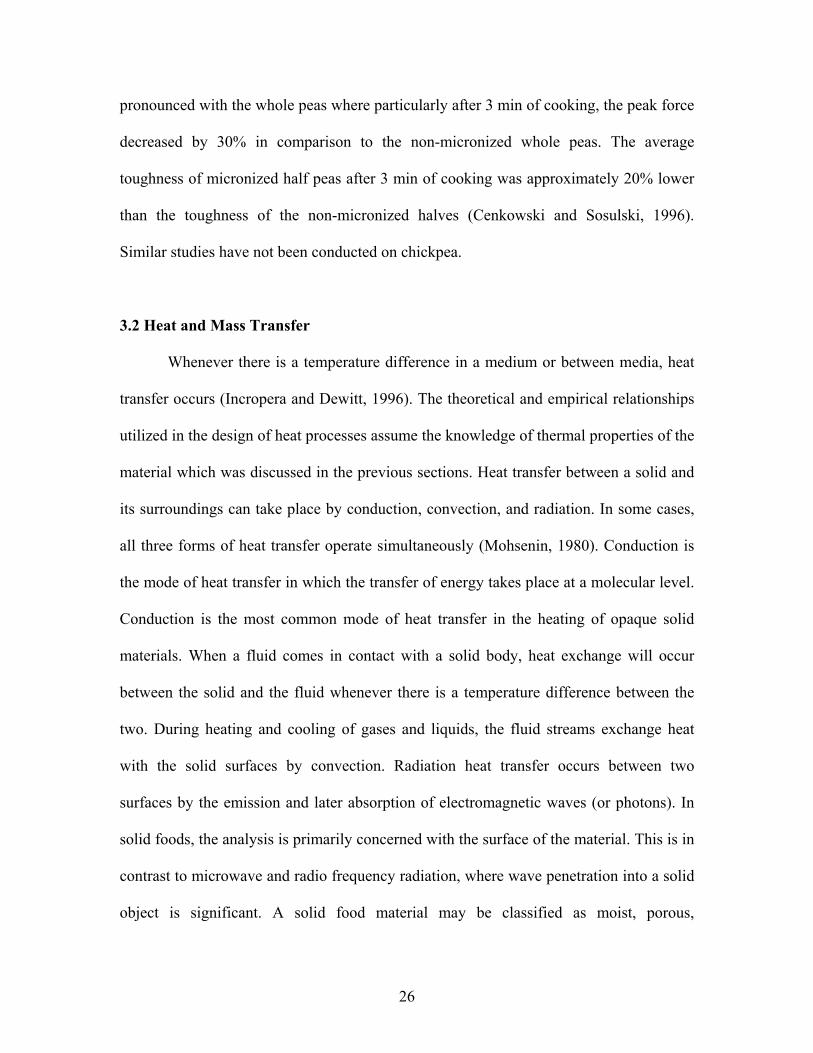
3.2 Heat and Mass Transfer

Whenever there is a temperature difference in a medium or between media, heat

transfer occurs (Incropera and Dewitt, 1996). The theoretical and empirical relationships

utilized in the design of heat processes assume the knowledge of thermal properties of the

material which was discussed in the previous sections. Heat transfer between a solid and

its surroundings can take place by conduction, convection, and radiation. In some cases,

all three forms of heat transfer operate simultaneously (Mohsenin, 1980). Conduction is

the mode of heat transfer in which the transfer of energy takes place at a molecular level.

Conduction is the most common mode of heat transfer in the heating of opaque solid

materials. When a fluid comes in contact with a solid body, heat exchange will occur

between the solid and the fluid whenever there is a temperature difference between the

two. During heating and cooling of gases and liquids, the fluid streams exchange heat

with the solid surfaces by convection. Radiation heat transfer occurs between two

surfaces by the emission and later absorption of electromagnetic waves (or photons). In

solid foods, the analysis is primarily concerned with the surface of the material. This is in

contrast to microwave and radio frequency radiation, where wave penetration into a solid

object is significant. A solid food material may be classified as moist, porous,

27

hygroscopic solid with low thermal conductivity. Such materials offer high resistance to

internal heat transfer (Adu and Otten, 1996).

Mass transfer plays a key role in food processing. If there are differences in

concentrations of constituents throughout a solution or object, there will be a tendency for

movement of material to produce a uniform concentration. Such movement may occur in

gas, liquid, or solid solutions. Movement resulting from random molecular motion is

called diffusion. In solid, there can obviously be no convection and all movement is by

molecular diffusion. Mass transfer occurs during various food processing operations like

humidification and dehumidification, dehydration, distillation, absorption, etc. The

driving force for mass diffusion is the concentration difference. The basic relationship is

called Fick’s law and can be written as follows (Singh and Heldman, 2001):

−=

dxdCDN a

A (3.14)

where:

NA = mass flux of species A (kg/s.m2),

Ca = concentration in mass per volume,

x = distance in the direction of diffusion, and

D = diffusion coefficient, or diffusivity.

Most of the heat and mass transfer modeling in terms of cooking have been

concentrated on specific food and biological products whereas, study on legumes seeds

have been limited to drying. Past studies did not take into account the effect of heat and

mass transfer characteristics during cooking of legume seeds.

28

3.3 Mathematical Modeling

Numerical solution techniques are usually easier than analytical techniques since

engineering problems involve ordinary or partial differential equations which may not be

solved with the analytical solution techniques. In food and bioprocess modeling, the finite

difference method is commonly used especially in solving partial differential equations.

The coupling of heat and mass transfer process necessitates the use of numerical

techniques to solve heat and mass transfer differential equations simultaneously. The

finite difference method (FDM) and the finite element method (FEM) are among the

numerical methods that are widely used to solve a system of differential equations

(Fasina et al., 1993). Irudayaraj and co-workers (1992) compared the temperature and

moisture predictions of different sets of coupled heat and mass transfer models. The

application was on the drying of soybean, barley, and corn. They reported that the

simulation results from the heat and mass transfer models agreed well with the available

experimental results.

A three dimensional non-linear finite element model involving variable diffusion

coefficients, thermal conductivities and specific heat was developed by Fasina and co-

workers (1993) in an expanding alfalfa cube during moisture adsorption and they

reported that the rate of moisture absorption was dependent upon the relative humidity

and temperature of the surrounding air.

Huang and Mittal (1995) developed a model, simulated and validated the heat and

moisture transfer phenomena within a meatball during different cooking processes to

predict the temperature and mass of the meatball. They reported that the average cooking

time of meatball, by boiling in water was 770 s. Bengtsson and co-workers. (1976)

29

studied the heat and mass transfer in beef roasts and reported that there is an inverse

relationship between the moisture and temperature histories.

Pavon-Melendez and co-workers (2002) studied the dimensionless analysis of the

simultaneous heat and mass transfer in food drying. The theoretical analysis and

experimental drying kinetics showed that in mango drying, the temperature evolution was

controlled by heat convection in the food-air interface and moisture loss was controlled

by water diffusion in the interior of food. Mulet (1994) studied the suitability of heat and

mass transfer equations simplifications for modeling the experimental drying kinetics of

carrots. He showed that a model with constant temperature and constant diffusivity fitted

the drying curves with minimal root mean square deviations. Baik and Mittal (2004)

developed mathematical models to describe moisture, fat and heat transfer during deep

fat frying of a tofu disc. The model developed was useful for the prediction of

temperature, moisture and fat content during tofu frying at different temperatures. They

proved that the methodology proposed to incorporate shrinkage is simple and applicable

for simulating the frying process of different food products.

Maroulis et al. (1995) modeled air drying of foods with simultaneous heat and

mass transfer equations solved numerically. They reported that a model with variable

diffusivity, interface resistance for heat and mass transfer, and with heat conductivity

negligible yield the optimum fit for potato experimental drying kinetics. A one-

dimensional finite difference modeling of heat and mass transfer during thawing of ham

was reported by Delgado and Sun (2003) and the results showed that the effect of the

uncertainty of thermo-physical properties on the prediction of thawing time was

important. A mathematical model using the finite difference technique was developed

30

for simultaneous heat and moisture transfer during drying of potato (Wang and Brennan,

1995). The model took into account the effect of moisture-solid interaction at the drying

surface by means of sorption isotherms of food. The model was successfullapplied to the

air drying potatoes.

Mathematical models developed so far have considered the transport properties of

either moisture or temperature in specific food products using microwave or infrared

techniques. Whereas heat and mass transfer properties during boiling of chickpea with

water has not been studied. Hence, an extensive study will be useful for further studies

being conducted in this area.

3.4 Summary

Research reviewed in this thesis indicated the available data for the physical and

thermal properties of chickpea. However, the thermo-physical properties of kabuli type

chickpea have not been reported so far. The composition, physical, and mechanical

properties of chickpea when subjected to different heat treatment methods was reported.

There is a lack of information on the heat and mass transfer characteristics of chickpea

and also on modeling of the cooking process. Numerical method for solving the heat and

mass transfer equations was discussed.

31

4. MATERIALS AND METHODS

Food thermal properties play an important role in the quantitative analysis of food

processing operations. An overview of the materials used and the experiments that were

conducted for the purpose of modeling are explained in this chapter. Measurement of

density, thermal conductivity, specific heat, grain temperature during cooking, water

absorption during soaking and moisture absorption during cooking are discussed. Solid

loss during soaking is also explained.

4.1 Material

Kabuli type chickpea (Cicer arietinum L.) were procured from Canadian Select

Grain (Eston, SK) and stored in a walk-in cold storage room at 5-7°C, located in the

Department of Agricultural and Bioresource Engineering, University of Saskatchewan.

4.2 Moisture Content Determination

Moisture content was determined for randomly selected grain using the AOAC

method (AOAC, 2002). Small aluminum pans were used in containing the sample for

moisture determination. About 2 to 3 g of Wiley mill-ground samples were taken and

weighed. The sample mass before drying was recorded and the sample was placed in the

oven at 130°C for 1 to 2 h. The samples were taken out, cooled in a dessicator and then

weighed again. The loss of weight in the sample was used to calculate the moisture

content of the sample (Equation 4.1); the initial moisture content of the sample was found

to be 9.86% w.b. The grains were conditioned to different moisture contents by drying or

32

rewetting them.

100×WW

=Ms

ww (4.1)

where:

Mw = moisture content of the sample (% w.b.),

Ww = mass of water (g), and

Ws = mass of the sample (g) before drying.

Dried samples having moisture content of 7% was obtained by drying in a forced-

air thin layer dryer at a temperature of 50°C. Rewetted samples ranging in moisture

content from 13 to 35% were obtained by spraying pre-determined amounts of distilled

water on the chickpea seeds, followed by periodic tumbling of the samples in sealed

containers. Grains of moisture content of 55% were obtained by fully soaking the seed in

distilled water for 12 h, and that of 65% was obtained by boiling the grains in water. The

moisture conditioned grains were stored in the walk-in cold storage room in airtight glass

containers for further experiments.

4.3 Density Measurement

Particle density is the density of a sample which has not been structurally

modified (Rahman, 1995). It includes the volume of all closed pores but not the

externally connected pores. Density is a physical property of a food material dependent

both on temperature and moisture content.

This experiment was carried out to determine the particle density of the seed at 7

levels of moisture content, namely 9.86, 13.20, 18.17, 25.10, 35.89, 55.97 and 65.24%

w.b., respectively. Density measurement was done in 5 replicates. The instrument used

33

for this experiment was the multipycnometer (Quantachrome Corporation, Boynton

Beach, FL) as shown in the Figure 4.1. It is the most versatile model and gained its name

from its multiple volume features that offers three sizes of interchangeable sample cells:

135, 20 and 4.5 cm3. In addition, there are three different calibrated reference volumes

which provide peak performance for each cell size. The operating sequence is that the

reference volume is pressurized and then the gas is expanded into the sample cell. The

very wide operating range of the multipycnometer offers the greatest sample flexibility in

the series, while it maintains a degree of accuracy. This instrument is specifically

designed to measure the true volume of various quantities of solid materials. The

technique employs the Archimedes principle of fluid displacement to determine the

volume. The displaced fluid is a gas which can penetrate the finest pores to assure

maximum accuracy. For this reason, helium is recommended since its small atomic

dimension assures penetration into crevices and pores approaching one Angstrom (10-10 m).

Its behavior as an ideal gas is also desirable. Other gases such as nitrogen can be used,

often with no measurable difference.

. Figure 4.1 Multipycnometer used for measuring particle density.

34

A schematic diagram of the gas multipycnometer is shown in Figure 4.2. It

determines the volume of samples by measuring the pressure difference when a known

quantity of nitrogen gas under pressure is allowed to flow from a precisely known

reference volume (VR) into a sample cell containing the solid or powdered material.

Figure 4.2 Schematic diagram of gas multipycnometer (Manual, Quantachrome

Corporation, Boynton Beach, FL)

The working equation is given as follows (Manual, Quantachrome Corporation,

Boynton Beach, FL):

1PP

VVV2

1Rcp −

−=

(4.2)

where:

Vp = volume of the particle (cm3),

Vc = volume of the cell (cm3),

VR = reference volume for the large cell (cm3),

P1 = pressure reading after pressurizing the reference volume (psi), and

P2 = pressure reading after including Vc (psi).

35

Prior to measuring the density of a sample, calibration for the pycnometer was

done to determine the reference volume of a large calibration sphere. Particle density

refers to the weight per unit volume of the grain kernel and was calculated using

Equation 4.3:

pVm

=ρ (4.3)

where:

ρ = density (kg/m3), and

m = mass (kg).

4.4 Thermal Conductivity

Thermal conductivity of food is an important property to be considered in

calculations involving rate of heat transfer. Materials of high thermal conductivity

dissipate heat faster than those of low thermal conductivity. Most high moisture foods

have thermal conductivity equal to that of water.

The objective of this experiment was to determine the thermal conductivity of

chickpea at 5 different moisture levels, namely 7.00, 9.86, 13.30, 18.17 and 25.10% w.b.

at temperatures 25.0, 40.0, 60.0, 80.0 and 98.7°C, respectively. This experiment was

conducted in triplicates using two probes, namely, the assembled probe and the thermal

properties analyzer.

4.4.1 Thermal conductivity measurement using the assembled probe

Thermal conductivity was determined using an assembled thermal conductivity

probe. The line source method was used to measure the thermal conductivity of chickpea.

36

The unsteady state method uses either a bare wire or a thermal conductivity probe as a

heating source, and estimates the thermal conductivity based on the relationship between

the sample core temperature and the heating time.

The probe method was used in measuring the thermal conductivity due to its ease

of use and accuracy (± 0.05ºC) in measurements. This probe method saves both energy

and time. Time taken to take a set of time-temperature data is around 2 min. The single-

needle probe technology reduces user error. It is a portable handheld device which can be

used in environments maintained at different ambient temperatures. The effects on the

thermal conductivity measurement using the probe can be negligibly small if the

instrument and the measurement procedure are adequately designed. Fine needle probe is

commonly used in determining the thermal conductivity of penetrable materials such as

fluids, fruit and animal flesh. The use has been extended in finding the thermal

conductivity of seeds.

Correction analysis of the dimension influence on the measurement accuracy of

thermal conductivities by transient probe method is made. The radial and axial lengths of

the measured sample, the radius ratio and heat capacity ratio of sample to probe, as well

as the length to diameter ratio of the probe are important parameters in error analysis.

4.4.1.1 Probe construction

The thermal conductivity probe used in this study was constructed of a brass

needle tubing (length of 91.52 mm and diameter of 2.02 mm) with a Type T

thermocouple inside the tubing. The tube was filled with high thermal conductivity paste

material. Bare constantan wire (diameter 0.1 mm) with insulation stripped at both ends

was utilized as the heater wire. A thermocouple wire was inserted into the probe to half

37

its length. The heater wire and the thermocouple wire were insulated from each other.

The heater wire was fed through the brass tubing until it emerged from the paste at the

opposite end. One end of the heater wire that emerged from the tubing was crimped and

soldered to the tip of the tubing. The other end of the heater wire was attached to the

power supply. A piece of heat shrink was attached to the end of the tubing to hold the

heater and the thermocouple wires in place. A diagram of the assembled probe is shown

in Figure 4.3.

Figure 4.3 Assembled probe for thermal conductivity measurement.

4.4.1.2 Measurement technique for assembled probe method

This method utilizes a constant heat source to an infinite sample body at a

uniform initial temperature along a line of infinitesimal diameter compared to the sample

body. Having the heat source imbedded in the sample, the line-source is energized and

the temperature rise at a given distance from the source is measured after a short heating

time. The maximum slope method of arriving at the thermal conductivity (k) values was

Solder

High Thermal Conductivity Paste

Heater wire (Constantan)

Brass Tubing

Thermocouple (Type T)

38

used (Wang and Hayakawa, 1993). This method involves finding the local slope

(temperature rise over ln (time)). The probe was calibrated in distilled water at room

temperatures of 23 to 24ºC.

A schematic diagram of the instrumentation for measuring thermal conductivity is

shown in Figure 4.4. The components of the system for thermal conductivity

measurement consisted of the power supply, thermal conductivity probe and the

datalogger. The heater wire of the probe was connected to the power supply and the

thermocouple wire was connected to the datalogger. The time-temperature data was

monitored using the datalogger which was collected using the system.

System

Power supply

ProbeHeater wire

Thermocouple

Datalogger

System

Power supply

ProbeHeater wire

Thermocouple

Datalogger

Figure 4.4 Schematic diagram of the thermal conductivity measurement.

In principle, the heat generated in a hot wire at a rate q (W/m) is given by:

RIq 2= (4.4)

where:

I = electric current (A), and

R = electric resistance (Ωm-1).

39

Equation 4.5 shows a linear relationship between (T - To) and ln (t) where k4

qπ

is the

slope (Yang et al., 2002).

( )tlnk4

qr21ln

k2q

k2qATT 2

1

0 π+

α

π−

π=−

− (4.5)

where:

T = sample temperature anywhere in the cylinder (°C),

T0 = initial sample temperature (°C),

t = time (s), and

r = radial axis (m),

Slope S can be obtained from linear regression, and the (T - To) versus ln (t) and thermal

conductivity can then be calculated from S:

4SRIk

2

= (4.6)

Due to non-ideal conditions during the experimental trials, such as non-zero mass

and volume of the hot wire, heterogeneous and anisotropic properties of biological

materials, finite sample size and axial heat flow (Mohsenin, 1980; Suter et al., 1975;

Wang and Hayakawa, 1993), temperature rise (T - To) versus ln(t) does not always follow

a linear regression relationship. This calls for correction during data analysis. The most

used early method for data correction was the time-correction factor method (van der

Held and van Drunen, 1949), which minimized the non-linearity of the (T - To) versus ln

(t) curve by subtracting a factor from the time elapsed. Underwood and McTaggart

(1960) proposed a method for time correction for finite probe diameter using the

following equation:

40

×

−π×

=1

2

12

2

tt

log3.2)TT(k4

414.3RIk (4.7)

where:

T2 and T1 = temperatures (°C),

t2 and t1 = time (s).

Equation 4.7 is the corrected equation for a probe with finite diameter. Murakami

and Okos (1988) proposed a method for a maximum coefficient of determination (R2) for

the correction, which searched for a maximum linear portion of the curve by successive

linear regression using R2 values as the criteria for the maximum linearity. Wang and

Hayakawa (1993) theoretically and experimentally verified the maximum slope method

that was first used by Asher et al. (1986). This method calculates the thermal conductivity

using the maximum slope around a plateau of the local slope versus ln (t) plot. The study

of Wang and Hayakawa (1993) showed that the thermal conductivities determined using

the maximum slope method is comparable or more accurate than the time-correction

method and the maximum R2 method.

4.4.1.3 Thermal conductivity of distilled water

The probe was calibrated in distilled water at room temperatures of 23 to 24ºC. A

1 L beaker was filled with distilled water and the probe to be calibrated was held in place.

The test was run for 40 to 50 s and the temperature was recorded every 0.25 s in the

Campbell Scientific CR10X datalogger (Campbell Scientific, Inc., Logan, UT). Three

trials were done for each temperature. The maximum slope method of arriving at the

thermal conductivity (k) values was used (Wang and Hayakawa, 1993). The maximum

slope was identified and the thermal conductivity as shown in Equation 4.8 was

41

calculated. For distilled water measurements, the local slope was determined by linear

regression analysis of around 20 values of ln (time) (x) and the temperature (y). A k value

determined by this method is the average temperature of the maximum line segment with

a temperature increase around this segment of less than 0.5ºC.

4.4.1.4 Thermal conductivity measurement of chickpea

Holes were bored on the chickpea using a drill bit. The diameter of the drill bit

was selected such that it was nearest to the diameter of the probe. Around 8 chickpea

seeds were inserted into the probe. Precautions were taken to assure the best contact

possible between the chickpea seeds and probe. Fortes and Okos (1980) found the

thermal conductivity of corn kernels using the probe method. They applied nail polish

between the kernels and on any visible metallic spot in order to prevent any undesirable

conduction. In this experiment, the probe with chickpea sample was vacuum packed in a

polyethylene bag and assumed to have negligible contact resistance. Figures 4.5 and 4.6

show the chickpea seeds during measurement of thermal conductivity. The grains when

tested for thermal conductivity at different temperature ranges were allowed to

equilibrate in the respective chamber before the experiments were conducted. The wires

connecting the heater in the probe were plugged to a power supply set to a constant

current supply of 0.665 A. Temperature data was recorded at every 0.25 s interval on the

datalogger (Campbell Scientific, Inc., Logan, UT). The probe resistance was measured to

be 5 Ωm-1. The temperature of the chamber was recorded by another thermocouple

connected to the data logger at 0.25 s interval.

42

Figure 4.5 Thermal conductivity probe with chickpea seed sample.

Figure 4.6 Measurement of thermal conductivity of chickpea.

The maximum slope method described previously was used to calculate the

thermal conductivity of chickpea. Local slope was determined by linear regression

43

analysis of 20 values of ln (time) (x) and probe temperature (y). The k value was

calculated using Equation 4.8 with the maximum slope calculated earlier.

π

′=

1

2

12 ttln

)T-T(k4qk (4.8)

where:

q' = I2R which is the heat input per meter length of the line source (W/m),

k = thermal conductivity (W/mK) of the medium infinite in size surrounding the heat source,

T = temperature (°C), and

t = time (s),

subscripts:

1 and 2 refer to any two points on a straight line resulting from the plot of temperature

versus ln (time).

4.4.2 Thermal conductivity measurement using the KD2 Thermal properties

analyzer

The thermal conductivity of the chickpea was also measured using the KD2

thermal properties analyzer (Decagon Devices, Inc., Pullman, WA) for temperatures

other than freezing, as its operating temperature was 5 to 35ºC. Figure 4.7 shows the

measurement of thermal conductivity of chickpea using the analyzer.

The probe length was 60 mm and its diameter was 0.90 mm Calibration of the

probe was done at temperatures of 20, 23 and 24ºC. This analyzer gives direct readings of

the thermal conductivity.

44

Figure 4.7 Measurement of thermal conductivity using the KD2 thermal properties analyzer.

4.5 Specific Heat

Specific heat is an essential property in the thermal analysis during food

processing such as heating or cooling of foods. With food materials, this property is a

function of its chemical composition, moisture content, temperature and pressure. In most

food processing applications, specific heat at constant pressure is used since pressure is

generally kept constant except in high pressure processing.

Specific heat was measured at seven levels of moisture content, namely 9.86,

13.20, 18.17, 25.10, 35.89, 55.97 and 65.24% w.b., respectively. Measurements were

done in triplicates for each moisture level. It was determined using two methods namely,

the indirect mixing method and the differential scanning calorimetry (DSC).

4.5.1 Assembled calorimeter

The principle of indirect mixing method is used in the assembled calorimeter

experiment. This method provides no direct contact between the sample and the

45

calorimetric fluid, thus, eliminating the heat of solution of dissolvable chemical entities

of food. The specific heat measured using the assembled calorimeter is only a function of

moisture content and not a function of temperature, since average temperature

(equilibrium temperature) is used. In this measurement, the sample is initially at low

temperature and the calorimetric fluid is at a high temperature.

4.5.1.1 Apparatus

The calorimeter consisted of two stainless steel dewar flasks (Cole Parmer

Instrument Co., Vernon Hills, IL). The assembled calorimeters are shown in Figures 4.8

and 4.9. Rubber seal rings were attached to the rims of the flask to provide a good seal.

The calorimeters were referred to as A and B. Calorimeter A had copper constantan (type

T) thermocouples attached to either side of the walls to measure the temperature of the

walls as well as the fluid.

Figure 4.8 Assembled calorimeters A and B.

46

Figure 4.9 Dewar flask with thermocouples attached.

In Figure 4.10, F1, F2, and F3 denote the thermocouple positions measuring the

temperature of the fluid, whereas W1, W2, and W3 denote the thermocouple positions

measuring the temperature of the walls of the calorimeter A. This kind of thermocouple

arrangement was made on either sides of the dewar flask A, named as ‘A’ side and ‘B’

side. The cover for the flasks consisted of inner plexiglass lids with rubber O-rings, and

outer cork lid for better insulation with a small opening to let in the thermocouple wire

which measures the temperature of the sample.

The thermocouples were connected to the Campbell Scientific CR10X datalogger

(Campbell Scientific, Inc., Logan, UT) to collect and record the data. Figure 4.11 shows

the special kind of packing gland that was used to insert the thermocouples inside the

samples. A Type-T thermocouple was placed inside the plastic screw shown in Figure

4.11. The wire was then sealed to the plastic screw with the help of epoxy (Devcon

Corporation, Wood Dale, IL) and clear silicone (Permatex Inc., Salon, OH) and allowed

to set for 12 h. These glues were water proof and very good sealants. This thermocouple

47

was then inserted into the nylon polyethylene bag through a small hole which was made

with the help of a solder, where the other end was connected to the datalogger. While

measuring the temperature for the samples one end of the thermocouple was connected to

the centre of the chickpea and the other end to the datalogger. The samples were held

inside calorimeter A during temperature measurements by suspending the sample pouch

along with the thermocouple wires into calorimeter A.

Figure 4.10 Diagram of the calorimeter used for measuring specific heat of chickpea.

Cork lid

Rubber stopper

Plexiglass lid

O-ring (rubber)

Rubber seal rings

Dewar flask

F1

F2

F3 W3

W2

W1 Thermocouples

48

Figure 4.11 Packing gland used to insert thermocouples into the nylon polyethylene bag.

Calorimeter B was another dewar flask with similar type of lids as calorimeter A, except

that it did not have the thermocouples attached to the flask. Calorimeter B was used in

order to keep water at a constant temperature which in turn was poured into calorimeter

A during specific heat measurements.

4.5.1.2 Heat capacity measurement of calorimeter

The heat capacity of the calorimeter was determined prior to measurement of

specific heat of the samples. Calorimeter B was filled with deionized water at 50°C and it

was placed in a chamber maintained at 37±1.5°C for 15-30 min. The calorimeter was

closed to prevent evaporation. Calorimeter A was prepared with a plastic pouch attached

with three thermocouples connected to the datalogger. When calorimeter B and the water

inside it achieved a constant rate of exchange with its environment, it was taken out and

the water was poured into calorimeter A. The datalogger was started when the water from

calorimeter B was poured into calorimeter A. Calorimeter A was sealed tightly and

shaken every 2 or 3 min. Figure 4.12 shows the setup during heat capacity measurements.

Locking Nut

Plastic washer

Rubber washer

Plastic screw

49

Figure 4.12 Experimental set up during heat capacity measurement.

After 30 min, the data logger was stopped and the weight of calorimeter A with

and without water was measured. The calorimeter, plastic pouch and the thermocouples

were thoroughly dried before measuring their dry mass. The mass of water used is mw.

From the time-temperature curve, along with the initial temperatures of calorimeter and

water, the heat capacity of the calorimeter was calculated using the following equation:

tdtdT

+T-T

)tdtdT

-T-T(mc=H

eeoc

eowewpw

c

(4.9)

where:

Hc = heat capacity of calorimeter (kJ/K),

cpw = specific heat of water (kJ/kgK),

mw = mass of water (kg),

Te = temperature of water when it reaches equilibrium with the calorimeter (K),

Toc = initial temperature of the calorimeter (K),

50

Tow = initial temperature of water (K),

dT/dt = rate of temperature change (from graph of time temperature) (K/min), and

te = time (min) when water reaches equilibrium with the calorimeter.

4.5.1.3 Specific heat measurement of chickpea using the assembled calorimeter

In this measurement method, whole chickpea seeds were used. It is the intent to

use the whole seeds because the characteristic changes of the whole chickpea seed is

considered when subjected to cooking. 50 g of chickpea seeds were placed inside a

polythene pouch which had three thermocouples attached to it and they were vacuum

packed in a single layer with the thermocouples inserted inside the seed at different

locations. The thermocouples were inserted inside the seed by boring small holes to the

center of the chickpea and the wires were glued to the seed with 5 min curing epoxy.

Figure 4.13 shows the sample in the pouch and Figure 4.14 shows the photograph of the

calorimeter during specific heat measurement of chickpea.

Figure 4.13 Sample in plastic pouch with thermocouples.

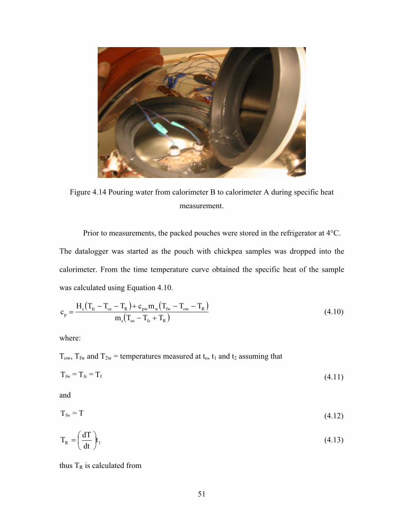
51

Figure 4.14 Pouring water from calorimeter B to calorimeter A during specific heat

measurement.

Prior to measurements, the packed pouches were stored in the refrigerator at 4°C.

The datalogger was started as the pouch with chickpea samples was dropped into the

calorimeter. From the time temperature curve obtained the specific heat of the sample

was calculated using Equation 4.10.

( ) ( )( )Rfsoss

RowfwwpwRocfccp TTTm

TTTmcTTTHc

+−−−+−−

= (4.10)

where:

Tow, Tfw and T2w = temperatures measured at to, t1 and t2 assuming that

T=T=T ffcfw (4.11)

and

T=Tfw (4.12)

1R tdtdTT

= (4.13)

thus TR is calculated from

52

t-tT-T

=T12

fww2R

(4.14)

According to Peralta et al. (1995), the choice of t1 and t2 are critical in estimating

the values of TR. The value of t1 was taken when the temperature of the water in the

calorimeter and that of the sample were within ±0.1°C from each other for the first time

and the value of t2 was taken 5 min after measuring t1.

4.5.2 Differential scanning calorimetry

The differential scanning calorimetry method was also used to determine the

specific heat of chickpea. Due to limited access of this instrument, only one set of

readings was taken for each level of moisture content. In this method, moisture and

temperature were considered as independent variables affecting the specific heat. This

method is based on measuring very small thermal effects produced in thermal processes.

The recorder in the system produces a thermogram showing any gain or loss of energy as

the sample is scanned at a given rate of temperature rise over a selected temperature

interval. The area inside the thermogram is proportional to the heat energy absorbed or

released by the sample during the heating or cooling process.

4.5.2.1 Apparatus

The differential scanning calorimetry (DSC) experiment described in this thesis

was performed using a temperature modulated DSC 2910 (MDSCTM, TA Instrument Inc.,

New Castle, DE) using a liquid nitrogen cooling accessory and a nitrogen gas DSC cell

purge. The DSC 2910 system allows both heating and cooling scans in the modulated or

non-modulated DSC regime. The DSC is a comparative device and must be calibrated.

53

The instrument was calibrated for specific heat capacity (cp) with sapphire as standard

reference. The reference value for cp was obtained from the manufacturer. Due to limited

access of instrument it was not calibrated with water. The data analyzer was Thermal

Analyst 2100 (TA Instruments, Inc., New Castle, DE).

4.5.2.2 Sample preparation for measurements

Sample moisture contents ranging between 18.17% and 55.97% w.b. were

obtained by soaking whole seeds with predetermined amount of distilled water. The

sample moisture content of 65.24% w.b. was obtained by fully cooking the seed. The

conditioned chickpea seeds were ground with the help of a blender, stored in small

airtight bottles and were allowed to equilibrate in the cold storage room at 5 to 7°C for

one week before measurements. Ground samples were used because the DSC was

capable of measuring the heat capacity for small quantity of sample ranging from 10-20

mg.The powdered samples prepared were at 6 levels of moisture content, namely 9.86,

18.17, 26.54, 37.89, 55.97 and 65.24%.

4.5.2.3 Specific heat measurement by the DSC

The DSC includes two heating discs which are in thermal contact with one

another and are isolated from the environment. Figures 4.15 and 4.16 show the

photographs of the DSC used and the sample holder, respectively. Two pans, in which,

one of the pans contains a sample and the other is an empty reference pan, were placed on

the discs in the holder.

Prior to testing, approximately 10 to 20 mg of sample was weighed and placed in

54

one of the small pan. This was hermetically sealed and dusted using a pressurized duster.

Heating both pans at a controlled, known rate and measuring the heat flow between them,

gave the differential in heat capacity of the reference pan and the sample.

Figure 4.15 Differential scanning calorimeter.

Figure 4.16 DSC sample holder.

Figure 4.17 shows the schematic of the DSC measurement. Figure 4.18 shows the

ground samples and the samples sealed in small aluminum pans.

55

Figure 4.17 Schematic of the DSC for specific heat measurement.

Figure 4.18 Ground samples and samples sealed in pans.

For specific heat measurements, the instrument raises the temperature of the

sample in the DSC cell at a constant heating rate. The heat flow rate into the sample is

determined according to the following equation (Widmann and Riesen, 1987):

dtmdTdtdQcp = (4.15)

where:

Resistance thermometer

Reference pan

Reference base

Sample pan

heater

Sample base

56

cp = heat capacity (kJ/kgK),

dQ/dt = heat flow rate (J/s),

dT/dt = heating rate (K/s), and

m = mass of the sample (g).

The temperature of the sample in the DSC cell increased at a constant heating rate

for measuring the specific heat of food. Factors that can affect the measured values of

biological materials are sample size, heating rate and sample sealing. The determination

of the specific heat using DSC is based on the assumption that during the test, the

temperature is uniform in the sample and the sample container. Temperature rise during a

DSC test increases the vapor pressure within the sample and as a result, moisture may

escape from the biological material in the form of water vapor. The latent heat absorbed

in the process may introduce error in the measurement. Thus, encapsulation or sample

pan sealing must be used to get good results (Mohsenin, 1980; Tang et al, 1991).

4.6 Thermal Diffusivity

The physical significance of thermal diffusivity is in determining how fast heat

propagates or diffuses through a material. The main application of thermal diffusivity is

to estimate the thermal processing time. It is a measure of the quantity of heat absorbed

by a material for a given temperature change, and further indicates the ability of the

material to conduct heat to adjacent molecules. The thermal diffusivity of chickpea was

calculated using the experimental values of specific heat, thermal conductivity and

density values from the following equation:

cρk

=αp

(4.16)

57

where:

k = thermal conductivity (W/mK),

ρ = particle density in (kg/m3), and

cp = specific heat of the chickpea (kJ/kgK).

The density values were obtained by experimentally determining the particle

density of the chickpea at different moisture contents using the gas pycnometer

mentioned earlier in this chapter.

4.7 Water Absorption During Soaking

This experiment was conducted to understand the moisture absorption

characteristics of chickpea grain at temperatures ranging from room temperature (24°C)

to cooking temperature namely 45, 60, 80, 98.7°C. Before each experiment, the samples,

containers and distilled water were kept in the desired temperature for a few hours to

reach to equilibrium. Samples were randomly hand selected excluding foreign materials

and broken, cracked and damaged grain. Ten grains were selected and weighed, then

placed in a glass beaker containing 200 ml distilled water. After every 1 h, the grains

were removed from the beakers and dried on a paper towel to absorb the excess water on

the surface and the mass loss was measured with the help of an electronic weighing

balance, and then returned to the beaker. The duration and the mass of the samples were

recorded manually. An experiment was terminated when the grain mass attained an

equilibrium value, that is when the incremental change in the sample mass was less that

0.001 g when measured after 1 h of soaking. Tests were done in three replicates.

58

4.8 Moisture Diffusivity Measurement During Cooking

Moisture diffusivity is an important transport property necessary for the design

and optimization of all the processes that involve internal moisture movement. This

experiment was conducted at cooking temperatures to determine moisture diffusion

during cooking of chickpea at temperatures of 70, 80, 90, and 98.7°C. Chickpea samples

of initial moisture content 9.86% and 55% w.b., were used. Prior to the experiments, the

samples were kept in the cold storage room.

4.8.1 Measurement of moisture diffusivity

The heat source was a thermostatically controlled hotplate. Distilled water (500

ml) was filled in an aluminum pan of diameter 21.5 cm and height 24.5 cm and heated by

the hotplate. Water temperature was maintained constant. 100 g of chickpea grain was

taken and soaked in the water. After every 1 h of soaking, the seeds were retrieved from

the pan, placed on tissue towel to remove excess water on the surface and placed in

plastic pouches and stored in the cold storage room for moisture content measurement.

This process was repeated until the seeds were cooked.

Moisture flow within a grain kernel takes place by diffusion. The transfer

coefficient is called as diffusion coefficient. Moisture diffusivity value was obtained by

applying Fick’s second law for species diffusion in a single phase, with boundary

conditions of internal resistance controlling uniform moisture content, integrated over the

volume of the slab (apple, mango) or sphere (strawberry) (Luikov, 1968). Moisture

diffusivity for a spherical grain with radial symmetry was calculated using the following

equation:

59

π−∑

π=

∞

=

222

1n22 X

9nexp

n16MR (4.17)

In the above equation, the average moisture content and the time are expressed as

dimensionless quantities.

where:

MR = moisture ratio, and

X = dimensionless time as shown in the following equations:

ei

e

MMMMMR

−−

= (4.18)

and

( )21

DtVAX = (4.19)

where:

M = moisture content of chickpea at time t during cooking (dry basis (% or decimal)),

Mi = initial moisture content (dry basis (% or decimal)),

Me = equilibrium moisture content (dry basis (% or decimal)).

A = surface area (m2),

V = volume of the kernel (m3),

A/V=3/radius for a sphere, and

D = diffusion coefficient (m2/h).

4.9 Temperature Measurement in the Center of Chickpea

This experiment was conducted in order to measure the cooking time of the

chickpea and also to determine the temperature at the center of the seed during cooking.

60

This data was used in verifying the modeling results. This experiment was conducted at

temperatures of 70, 80, 90 and 98.7°C at two levels of sample moisture contents namely,

9.86% and 55% w.b., for the unsoaked and soaked grain, respectively.

4.9.1 Sample preparation

Chickpea of uniform size of approximately 10 mm diameter were taken from the

cold storage room and selected randomly. This experiment was conducted in triplicates

for both soaked and unsoaked grain. Soaked grains were obtained by soaking the

chickpea grains for 12 h at room temperature in airtight containers in the cold storage

room, prior to experiments.

4.9.2 Temperature measurement

In order to measure the temperature of the centre of chickpea grain, a small hole

was made using a drill bit to the centre of the grain. Thermocouples that were used for

measuring the centre temperature of chickpea were of 0.5 mm in diameter copper-

constantan wires (Type T) encased in Teflon tubing. They were further connected to

thermocouple wires of bigger diameter. One end was glued to the centre of the grain and

the other end was connected to the CR10X datalogger (Campbell Scientific, Inc., Logan,

UT). Three seeds were selected randomly for each run of experiment. The thermocouples

were inserted in the bored holes and they were sealed with epoxy and silicon glue and left

for 24 h to dry. To prevent moisture evaporation, they were sealed in plastic pouches.

Heat source was a hotplate which was controlled with a thermostat and the pan used was

made of aluminum having a diameter of 21.5 cm and a height of 24.5 cm. Distilled water

61

was filled in the pan and heated. The water temperature was maintained constant to

within ± 0.05°C. Two instrumented chickpea seeds were suspended in the water and

cooked along with 100 g of chickpea. They were cooked without lid. Temperature data

was recorded with time with the help of the datalogger. Periodically, a chickpea seed

were removed with the help of a small strainer and squeezed with the help of fingers to

see if they were cooked. Once the grains were cooked, they were removed. This

experiment was repeated for different temperatures namely 70, 80, 90 and 98.7°C for

both the unsoaked and soaked grain.

4.10 Solid Loss During Cooking

This experiment was conducted to determine the mass loss during soaking and

cooking of chickpea. It was conducted at temperatures of 25, 40, 60, 80, 98.7°C.

4.10.1 Solid loss measurement

Samples with initial moisture content 9.86% were used, and approximately 25 g

of grain were weighed for each experiment. For this experiment, a 500 ml glass dish was

used. The mass of the empty dish was recorded prior to adding water. Water (200 ml)

was poured into the dishes and the dish was placed in the chamber to maintain a constant

temperature and the previously weighed grain was soaked in the dish for 12 h. Soaking at

25, 40 and 60°C were done in chambers maintained at these required temperatures; and

the cooking temperatures of 80 and 98.7°C were obtained by placing the container in the

hotplate controlled with a thermostat. After 12 h, the soaked and cooked grains were

removed, the remaining water and the solids were evaporated at low temperatures and the

62

mass was taken. The mass difference of the dish with the dried mass and the empty dish

was considered as the amount of solid loss during soaking and cooking. Figures 4.19 and

4.20 show the soaking of grain and the evaporated solids in the dish after removal of the

grain, respectively.

Figure 4.19 Soaked chickpea.

Figure 4.20 Solid loss during soaking.

63

5. MODELING AND SIMULATION

In this chapter, the partial differential equations for temperature and moisture

distribution used for the modeling and the finite difference formulation and the solution

methodology to obtain the result are explained. A brief detail of the simulation program

is also mentioned.

This chapter reviews the modeling of the cooking process. Finite difference

method was used to solve the mathematical equations and simulation was carried out

using suitable software, the Interactive Simulator (ISIM) Rev 2.06 simulation

programming (Dunn et al., 1992). In the context of food processing, a mathematical

model involves an approximate representation of a process in mathematical terms. In

many cases, such as in biological systems, where the material is a poor conductor of heat,

the mathematical model for a real time system cannot be solved analytically, thus,

computer simulation is used. This is best characterized with the Biot number which

provides a measure of the temperature drop in the solid relative to the temperature

difference between the surface and the fluid. The solutions to these equations are

supposed to simulate the natural behavior of the material.

Cooking is an important form of heat treatment in the food industry because of

such advantages as simplicity of equipment and consumer preference. Factors such as

raw material, cooking time of the grain, and the initial moisture content of the sample

will affect the final product temperature and moisture content. The optimum combination

of these factors can be obtained by complete experimentation or by use of computer

modeling and simulation with subsequent verification of the models by experimental

64

results.

Heat may be transferred by one or more of the three mechanisms of conduction,

convection and radiation. Figure 5.1 shows the directions of heat and mass flow during

cooking of chickpea based on the assumptions mentioned below.

Figure 5.1 Direction of heat and mass flow during cooking of chickpea

5.1 Assumptions in Modeling

The following assumptions were made:

1) heat and moisture transfer is one dimensional, unsteady state in the radial direction;

2) chickpea is considered to be an almost spherical object;

3) the initial temperature and moisture distributions are uniform;

4) there is a temperature and moisture gradient in the chickpea with respect to time;

5) the thermal properties are constant;

6) chickpea is considered as a homogeneous isotropic solid;

Convection

Heat conduction

Moisture movement

Moisture diffusion

65

7) heat is transferred to the surface by convection and to the geometric center of the seed

by conduction;

8) moisture transfer to and from the seed is due to concentration gradient;

9) the amount of solid loss in the grains during cooking was neglected.

Based on the above assumptions, the mathematical models characterizing one

dimensional heat and moisture transfer in a chickpea grain during cooking was

investigated.

5.2 Governing Equations and Boundary Conditions for Heat and Mass Transfer

The system of equations and the associated initial and boundary conditions used

to describe the heat and moisture transfer process in the cooking of chickpea seeds, based

on the assumptions made above are given in the following subsections.

5.2.1 Heat and mass transfer

In food process engineering, heat transfer is very often in the unsteady state, in

which temperatures are changing and materials are warming or cooling. Unfortunately,

the study of heat flow under these conditions is complicated. There are some cases that

can be simplified and handled by elementary methods, and charts have been prepared

which can be used to obtain numerical solutions under some conditions of practical

importance. A simple case of unsteady-state heat transfer arises from the heating or

cooling of solid bodies made from good thermal conductors.

Heat transfer is the process whereby heat flows from regions of higher to regions

of lower temperature. Unsteady-state (or transient) heat transfer is that phase of the

66

heating and cooling process when the temperature changes as a function of both location

and time. In food process operations, the unsteady-state period is an important component

of the process. Analysis of temperature variations with time during the unsteady-state

period is essential in designing such a process.

Temperature is a function of two independent variables, time and location, hence

the following partial differential equation is the governing equation for a one dimensional

case.

∂∂

∂∂

ρ=

∂∂

tTr

rrck

tT n

np

(5.1)

where:

T = temperature (°C),

t = time (s),

r = the distance from centre location (mm).

Equation 5.1 can be expressed for different geometrical shapes using

n = 0 for slab,

n = 1 for cylinder, and

n = 2 for sphere.

The combination of properties pc

kρ is defined as thermal diffusivity, α. The

general equation of heat transfer at a constant α for a spherical object is given as

∂∂

+∂∂

α=∂∂

rT

r2

rT

tT

2

2

(5.2)

where:

α = thermal diffusivity (m2/s).

67

Diffusion is the process by which matter is transported from one part of a system

to another as a result of random molecular motions. General solutions of the diffusion

equation can be obtained for a variety of initial and boundary conditions provided the

diffusion coefficient is constant. If the diffusion is radial, the diffusion equation for a

constant diffusion coefficient in a spherical system takes the form of:

∂∂

+∂∂

=∂∂

rC

r2

rCD

tC

2

2

(5.3)

where:

D = diffusion coefficient (m2/s),

C = concentration (kg/kg), and

r = radial distance from the center of the seed (m).

5.2.2 Initial and boundary conditions

The boundary conditions are specified at the center and surface r = 0 and r = r0 for

a one dimensional system. Heat transfer is in the positive radial direction with

temperature distribution, which may be time dependent designated as T(r, t). The first

condition corresponds to a situation for which the surface is maintained at a fixed

temperature, Ts, since the surface is in contact with the boiling liquid.

The initial temperature and moisture distribution are assumed to be uniform. The

initial condition for the distribution of temperature is specified as:

0T)0,r(T = (5.4)

at the center for symmetric heating condition:

0tT

0r

=∂∂

=

(5.5)

68

Due to heat transfer at the surface of the seed by convection and to the geometric

center of the seed by conduction the boundary condition for heat transfer is given by the

following equation (Huang and Mittal, 1995):

)TT(hrTk sa

Rr

−=∂∂

=

(5.6)

where

h = heat transfer coefficient (W/m2K),

Ta = ambient water temperature (K), and

Ts = surface temperature of the chickpea (K).

The initial and boundary condition for the movement of moisture is given as:

0M)0,r(M = (5.7)

at the center:

0t

M

0r

=∂∂

=

(5.8)

Convective mass transfer was assumed to be negligible since no external force

was used to stir and enhance the cooking process. Moisture content at the surface of the

chickpea seed was assumed to be in instantaneous equilibrium with that of the

environment (Huang and Mittal, 1995; Williams and Mittal, 1999; Ateba and Mittal,

1994). In this surface convection condition, if the mass transfer Biot number is much

larger than unity, the resistance to mass transfer by diffusion is much larger than the

resistance to transfer by convection. Taking this situation into account, the surface

concentration of the seed may be replaced by the concentration of the cooking medium

(water) Incropera and DeWitt (1996).

69

The boundary condition of the moisture content equilibrium of the chickpea

surface with the boiling water is expressed by (Huang and Mittal, 1995):

0RrMM =

= at t>0 (5.9)

es MM = (5.10)

where:

Ms = moisture content at the surface of chickpea (dry basis (%) or decimals)

Me = equilibrium moisture content at the surface of chickpea (dry basis (%) or decimals)

Due to diffusion and convection at the surface, mass transfer equation is given as:

)cc(hr

MD swmRr

m −=∂∂

=

(5.11)

where:

Dm = diffusive mass transfer coefficient (m2/s),

hm = surface mass transfer coefficient (m2/s),

cs = concentration of water in the seed (kg/m3),

cw = concentration of water (1000 kg/m3), and

M = moisture concentration (kg/kg).

5.3 Non-dimensional Analysis

Temperature, moisture content and the radial length were written in non-

dimensional form in order to simplify the numerical calculations. The dimensionless

temperature (θ) is defined as:

oa

o

TTTT

−−

=θ (5.12)

where:

70

T = temperature of the chickpea at any time during cooking (°C),

Ta = temperature of water (°C), and

To = initial or center temperature (°C).

The moisture ratio MR expressed in Equation 4.18 can also be referred to as the

dimensionless moisture concentration C as given below:

CMR = (5.13)

The dimensionless radial length (Ψ) is defined as:

Rr

=ψ (5.14)

where:

r = radial position (m), and

R = radius of the chickpea (m).

The heat and mass transfer equations explained above, in non dimensional form

can be expressed as:

ψ∂θ∂

+ψ∂θ∂

ψα

=∂θ∂

2

2

2

2Rt

(5.15)

ψ∂∂

+ψ∂∂

ψ=

∂∂

2

2

2m CC2

RD

tC (5.16)

( ) 10, =ψθ ; (5.17)

( ) 10,C =ψ ; (5.18)

00

=ψ∂θ∂

=ψ

; (5.19)

0C

0

=ψ∂∂

=ψ

; (5.20)

71

( ) )TT(hR

TTksa

oas −=ψ∂−θ∂ (5.21)

Cs = 1 at t>0 for boiling

where:

Cs = concentration at the surface of the chickpea, and

t = time, s.

5.4 Solution Method

The solution method used to solve the finite difference equations is explained in

this section. The equations are discretized to simplify the calculations and simulation.

5.4.1 Development of finite difference equations

A one-dimensional spherical finite difference framework, consisting of 10

concentric shells of equal thickness, was developed to model the heat and moisture

concentration in a chickpea during cooking.

Figure 5.2 Position of nodes in the chickpea.

0

9

2

1011

431

72

Eleven nodes in total, one at the center of each shell element and the 11th on the

outer surface, were assigned. Temperature and moisture content at each of these nodes

were assumed to be representative of the entire element. The position of the nodes taken

is shown in Figure 5.2. The geometric center is represented by node 0 and the surface

node by 11. All the other nodes are a representative of the entire element that has been

divided from 1 to 10.

5.4.2 Discretization of the equations

In the finite difference approach, the problem domain is ‘discretized’ so that the

dependent variables are considered to exist only at discrete points. The difference

representation given in the following equations were automatically solved by the

software. Only one unknown appears in the difference equation in a manner that permits

evaluation in terms of known quantities. Derivatives are approximated by differences

resulting in an algebraic representation of the partial differential equation.

Node 0 (Geometric center)

Using the boundary condition and the central difference:

( )0120

R300

dtd

θ−θα

=θ (5.22)

( )012m0 CC

RD300

dtdC

−= (5.23)

Nodes 1-9

Using the central difference

For temperature:

73

( )

θ+θ−θ+

θ−θψ

α=

θ −+−+

−=2

1ii1i1i1i

i2

91i

i

1012

1022

Rdtd

(5.24)

( )1221 23

R100

dtd

θ−θα

=θ (5.25)

θ+θ−θ

α=

θ1232

2

312

35

R100

dtd

(5.26)

θ+θ−θ

α=

θ2342

3

532

57

R100

dtd

(5.27)

θ+θ−θ

α=

θ3452

4

752

79

R100

dtd (5.28)

θ+θ−θ

α=

θ4562

5

972

911

R100

dtd

(5.29)

θ+θ−θ

α=

θ5672

6

1192

1113

R100

dtd

(5.30)

θ+θ−θ

α=

θ6782

7

13112

1315

R100

dtd

(5.31)

θ+θ−θ

α=

θ7892

8

15132

1517

R100

dtd

(5.32)

θ+θ−θ

α=

θ89102

9

17152

1719

R100

dtd

(5.33)

θ

−−

+θ−θ−+α

=θ

−+−=

1ii1i292i

i

1i23i22

1i21i2

R100

dtd (5.34)

Node 10 (near the surface), By both backward and central difference:

+

θ−θ−

θ−θ

++θ−θ

ψα

=θ

2

2Rdt

d

201

101

101

910

201

10s

201

101

9s

i2

10 (5.35)

74

θ+θ−θ

α=

θ910s2

10

5717

5740

R400

dtd

(5.36)

For moisture concentration:

( )

+−+

−ψ

= −+−+

−=2

1ii1i1i1i

i2m

91i

i

101CC2C

102CC2

RD

dtdC (5.37)

( )1221 C2C3

R100

dtdC

−α

= (5.38)

+−= 1232

m2 C31C2C

35

RD100

dtdC

(5.39)

+−= 2342

m3 C53C2C

57

RD100

dtdC

………………………… (5.40)

−−

+−−+

= −+−=

1ii1i2m

92i

i C1i23i2C2C

1i21i2

RD100

dtdC (5.41)

Node 10 (near the surface)

+−

α= 910s2

10 C5717CC

5740

R400

dtdC

(5.42)

Node 11(surface)

By backward difference:

The heat transfer equation for the surface node of zero volume can be formulated using

the boundary conditions as follows:

)(hr

k saRr

θ−θ=∂θ∂

=

(5.43)

)(kh

r saRr

θ−θ=∂θ∂

=

(5.44)

)(kh

2r sa

10s θ−θ=∆

θ−θ (5.45)

75

Thus, for surface node:

∆+

θ+θ∆

=θ

kh

2r1

kh

2r

10a

s (5.46)

5.5 Properties Used in Model Calculations

Constant properties namely, the heat transfer coefficient and mass transfer

coefficient that involved in the heat and mass transfer modeling is discussed in this

section.

5.5.1 Surface heat transfer coefficient (ht)

The heat transfer coefficient is the property of convective heat transfer systems

involving a solid surface and a fluid. It is one of the most important parameters necessary

to design and control of food processing equipment where fluids (air, nitrogen, steam,

water or oil), used as heating, cooling, frying, or cooking media. The surface heat

convection coefficient depends on the thermo-physical properties of fluid and solid

(density, specific heat, thermal conductivity). Convection is the most common means of

heat transfer used for heating solid food stuffs.

5.5.2 Calculation of convective heat transfer coefficient

For the calculation of the convective heat transfer coefficient, the lumped body

model was used. Aluminum balls of 9.51mm diameter were made to the size of chickpea

were used to calculate the surface convection coefficient. The thermal conductivity of

aluminum ranges from 230 to 240 W/mK.

76

Figure 5.3 Aluminum sphere and chickpea seed during measurement of heat

transfer coefficient.

Holes were bored to the center of the aluminum balls. A thermocouple wire was

inserted and sealed with epoxy glue. This was placed in boiling water and the time-

temperature data was collected. The temperature of the surrounding fluid was maintained

constant throughout the process. This approximation can be made when the following

condition in Equation 5.47 is satisfied (Incropera and DeWitt, 1996):

1.0k

hLBi ≤= (5.47)

where:

Bi = Dimensionless parameter Biot number,

h = convective heat transfer coefficient (W/m2K),

k = thermal conductivity of aluminum (W/mK), and

L = r/3 for a sphere (m).

For a lumped body, the temperature of the solid which is introduced into the fluid at time

t = 0 is given by:

( )

−=

−−

∞

∞ tmchAexp

TTTtT

pi

(5.48)

where:

77

Ti = initial temperature of the aluminum sphere (K),

T∞ = initial temperature of the aluminum sphere (K),

T(t) = temperature at any time t (K),

A = surface area of the solid (m2),

cp = specific heat of aluminum (J/kgK),

m = mass of aluminum sphere (kg),

h = heat transfer coefficient (W/m2K), and

t = time (s).

5.5.3 Diffusion coefficient (Dm)

Diffusion coefficient is the factor of proportionality representing the amount of

substance diffusing across a unit area through a unit concentration gradient in unit time.

Estimates of diffusion coefficient were obtained from experimental data using the

sorption method with constant diffusion coefficient as outlined by Crank (1975). The

moisture diffusion coefficient was calculated from Equation 4.17. This method is based

on the assumption that the concentration at the surface of material when placed in a

humid environment reaches equilibrium and remains constant thereafter (Fasina et al.,

1993). For further calculations and modeling, the constant Dm value was used.

78

6. RESULTS AND DISCUSSION

This section of the thesis presents the experimental results obtained and the

discussions of the results. The experimental results are compared with the simulated

results.

6.1 Moisture Content

The moisture content of the whole grain chickpea samples selected randomly was

adjusted to seven levels by drying, rewetting, soaking and cooking. The chickpea

moisture content data are listed in Table 6.1 together with the mean, standard deviation

and the coefficient of variation. The moisture content values obtained in replicates are

shown in Table F1.

Table 6.1 Moisture content of chickpea seed samples used in experiments.

Level Moisture content Mean (% w.b.) *SD (% w.b.) **CV (%)

1 9.86 0.15 1.55 2 13.20 0.26 1.98 3 18.17 0.02 0.13 4 26.54 0.05 0.22 5 37.89 0.13 0.35 6 55.97 0.33 0.60 7 65.24 0.31 0.48 * Standard Deviation (n = 3) ** Coefficient of Variation

The standard deviation values ranged from 0.02 to 0.33% w.b. and the coefficient

of variation was found to be between 0.13 to 1.98%, which shows the accuracy of the

results obtained from the moisture content determination experiment.

79

6.2 Density

The particle density of the chickpea was measured using the gas pycnometer.

Table 6.2 shows the results that were obtained. Table F2 shows the density values that

were obtained during each trial. Before measuring the volume, the samples were sealed in

airtight glass containers. Loss of moisture during the experiment must be taken into

consideration. The samples when removed from the containers were transferred to the

pycnometer cell immediately. The actual weight of the sample was less than the weight

indicated when it was weighed. This may be due to the successive volume determinations

yielding results trending in one direction where contaminants are removed after each

depressurization. To reduce error, measurements were continued for five determinations

for each level of moisture content. The pressure transducer used in this pycnometer

dissipates a very slight amount of heat. Because of its extreme sensitivity, it can track a

slight pressure increase associated with the heating of the gas. Accordingly, it is

necessary to take the first reading observed after the digital display stabilizes. A change

of approximately 0.001 on the digital display every 10-20 s is indicative of pressure

increase due to heat dissipation and is normal. The most accurate and rapid results will be

achieved by taking the first reading after the display stabilizes and then rotating the

selector valve again and again immediately obtaining the first stable reading (Operating

Manual, Quantachrome Corporation, 1900 Corporate Drive, Boyton Beach, FL 33426).

It was observed from the results that there was a decrease in the density of the

chickpea for increased moisture contents. The kernel density of rewetted chickpea seeds

were reported by Konak and co-workers (2002) for moisture content ranging from 5.2 to

16.5% d.b., the kernel density decreased from 1428 to 1368 kg/m3 respectively.

80

Table 6.2 Particle density of chickpea as a function of moisture content.

Moisture content Density (% w.b.) Mean (kg/m3) SD (kg/m3) CV (%)

9.86 1459.44 19.07 1.31 13.20 1395.06 21.63 1.55 18.17 1384.18 21.05 1.52 25.10 1345.20 11.04 0.82 35.89 1305.51 9.19 0.70 55.97 1202.11 10.21 0.85 65.24 1109.82 3.36 0.30

n = 5

Dutta et al. (1988a) reported in their studies for moisture range from 9.64 to

31.0% d.b. that the kernel density of rewetted chickpea ranged from 1311 to 1257 kg/m3.

The same kind of trend was observed in the density values obtained in this experiment.

As the initial moisture content was increased from 9.86 to 65.24% w.b., the density

values decreased from 1459.44 to 1109.82 kg/m3. Figure 6.1 shows the plot for particle

density and seed moisture content.

PD = 1494.22- 5.54MR2 = 0.97

0

200

400

600

800

1000

1200

1400

1600

0 10 20 30 40 50 60 70

Moisture content (% w.b.)

Seed

den

sity

(kg/

m3 )

Figure 6.1 Seed density as a function of seed moisture content.

For moisture content of 65% w.b., the density was close to that of water. Equation

81

6.1 is the simple regression equation which was developed for particle density (PD) as a

function of moisture content:

M54.522.1494PD −= (6.1)

where:

M = moisture content (% w.b.).

The coefficient of determination (R2) was found to be 0.97. The standard error of

estimates was found to be 351.87 and the mean absolute deviation was found to be 17.04.

The standard deviation ranged from 3.36 to 21.63 kg/m3 and the coefficient of variation

ranged from 0.30 to 1.55% which show the accuracy of the results obtained.

6.3 Thermal Conductivity

The thermal conductivity of chickpea was determined using the assembled probe.

Thermal conductivity of distilled water was measured to calibrate the probe. Data was

collected at 0.25 s intervals for over 40 to 50 s. Figure 6.2 shows a typical temperature

history curve for distilled water at 25ºC. It was observed that there was a rapid rise in

temperature at the beginning and the curve levelled off to a plateau after a certain period

of time. The maximum slope was used to calculate the thermal conductivity. The k values

ranged from 0.5641 to 0.5967 W/mºC. The thermal conductivity of water at 25ºC is

approximately 0.6054 kJ/kg ºK (Beaton and Hewitt, 1989). Data for thermal conductivity

measurement of chickpea was collected at 0.25 s intervals for over 100 s. Heating was

rapid for the first 20 seconds as shown in Figure 6.3. The rate of rise in temperature

became constant. The thermal conductivity of chickpea increased with increasing

moisture content because of high thermal conductivity of water, ≈ 0.60 W/m°C.

82

0.0

0.5

1.0

1.5

0 1 2 3 4 5 6 7 8 9 10

ln (Time, s)

(T -

T 0) (

o C)

Figure 6.2 Typical experimental temperature history of distilled water at an initial

temperature of 25ºC; T = temperature at any time (ºC) and To = initial temperature (ºC).

0

1

2

3

4

0 5 10 15 20 25

Time (s)

(T -

T 0) (

o C)

Trial 1Trial 2Trial 3

Figure 6.3 Typical temperature history curve for chickpea during measurement of

thermal conductivity.

Table 6.3 shows the thermal conductivity mean values of kabuli chickpea at

moisture content of 7.00 to 25.10% w.b., and temperature of 25 to 98°C. Table F3 gives

the thermal conductivity values obtained during different trials. The slight deviations

between the trials may be due to some axial flow errors and probe diameter errors which

have been corrected to a maximum extent. It was observed that the thermal conductivity

83

increased with increase in moisture content and temperature as shown in Fig 6.4. The

values of thermal conductivity ranged from 0.1535 to 0.3257 W/m°C. The accuracy of

the values was found by regression analysis. The standard deviation values obtained

ranged from 0 to 0.0045 and the coefficient of variation ranged from 0.02 to 2.44%,

which shows the accuracy of the results obtained. The thermal conductivity of borage

seeds for moisture content ranging from 1.2 to 30.3% w.b., were reported to be 0.11 to

0.28 W/m°C by Yang and co-workers (2002).

Table 6.3 Determination of thermal conductivity using the assembled probe.

K (W/m °C) CV k model Temp (°C)

M.C (% w.b.) Mean SD (%) (W/m °C)

25 7.00 0.1535 0.0006 0.39 0.1633 25 9.86 0.1849 0.0045 2.44 0.1795 25 13.20 0.2163 0.0009 0.42 0.1985 25 18.17 0.2365 0.0019 0.78 0.2268 25 25.10 0.2456 0.0011 0.48 0.2662 40 7.00 0.1694 0.0002 0.02 0.1757 40 9.86 0.1966 0.0020 1.04 0.1920 40 13.20 0.2294 0.0006 0.26 0.2110 40 18.17 0.2491 0.0009 0.39 0.2392 40 25.10 0.2637 0.0004 0.16 0.2787 60 7.00 0.1795 0.0005 0.30 0.1923 60 9.86 0.2029 0.0006 0.32 0.2086 60 13.20 0.2393 0.0009 0.38 0.2276 60 18.17 0.2632 0.0034 1.29 0.2558 60 25.10 0.2863 0.0007 0.26 0.2952 80 7.00 0.1886 0.0009 0.52 0.2089 80 9.86 0.2132 0.0012 0.59 0.2252 80 13.20 0.2529 0.0005 0.22 0.2442 80 18.17 0.2804 0.0007 0.25 0.2724 80 25.10 0.3001 0.0026 0.89 0.3118 98 7.00 0.2137 0.0023 1.11 0.2255 98 9.86 0.2343 0.0017 0.76 0.2417 98 13.20 0.2842 0.0016 0.58 0.2607 98 18.17 0.3091 0.0008 0.26 0.2890 98 25.10 0.3257 0.0004 0.15 0.3284

n = 3

84

The k values of borage seeds were slightly less than that of the thermal

conductivity values of chickpea seed. The value of thermal conductivity increased with

increasing temperature and moisture content. The magnitude and trend of the thermal

conductivity of chickpea samples versus increasing moisture content were in agreement

with the literature.

0.00

0.05

0.10

0.15

0.20

0.25

0.30

0.35

0 5 10 15 20 25 30

Moisture content (% w.b.)

Ther

mal

con

duct

ivity

(W/m

o C)

25°C45°C60°C80°C98°C

Figure 6.4 Thermal conductivity of chickpea as a function of moisture content and

temperature.

Deshpande and co-workers (1996) observed a linear increase in bulk thermal

conductivity of soybean from 0.1157 to 0.1756 W/m°C at 27°C in the moisture content

range between 8 and 25% d.b. Shepherd and Bhardwaj (1986) reported that the bulk

thermal conductivity of pigeon pea linearly increased from 0.1358 to 0.1862 W/m°C in

the moisture content range of 8 to 26% d.b., and temperature range 10 and 40°C. The

thermal conductivity of chickpea seeds was comparable with that of whole rapeseed

85

(0.108 to 0.155 W/m°C) at moisture contents from 6.1 to 12.8% w.b. and temperature 4.4

to 31.7°C (Mohsenin, 1980). The thermal conductivity values of alfalfa cubes were

higher than chickpea and ranges from 0.31 to 0.48 W/mK at 4.8 to 57°C (Khoshtaghaza

et al., 1995). The thermal conductivity value of chickpea seeds were higher than those of

whole peanut kernels (Suter et al., 1975) and whole soybean seeds (Mohsenin, 1980),

respectively.

The coefficient of determination R2 for Equation 6.2 expressing the dependence

of thermal conductivity to temperature and moisture content was 0.91 and a very small

standard error of 0.0125, which shows the accuracy of the values. The variables moisture

content, M (% w.b.) and temperature, T (°C) were analyzed with multiple linear

regression using MS Excel (Microsoft Corporation, Redmond, WA).

M0056.0T0008.01027.0k ++= (6.2)

The thermal conductivity was also determined using the KD2 thermal properties

analyzer. The k of water determined was in a range of 0.55 to 0.60 W/m°C which was

within the range given for water (Beaton and Hewitt, 1989). Chickpea seeds were

inserted into the probe after drilling it to almost an equal diameter of the probe. The

readings were taken for room temperature and the values of thermal conductivity were

found to range from 0.16 to 0.32 W/m°C for moisture contents of 7.00 to 25.10% w.b.

6.4 Specific Heat

Specific heat results were obtained by two methods namely, the assembled

calorimeter method and the DSC. In this section, the results obtained from both methods

are discussed.

86

6.4.1 Assembled calorimeter method

The heat capacity of the assembled calorimeter was determined using equation

4.15 and was found to be 0.4568 kJ/kg°C. Figure 6.5 shows the time-temperature curve

obtained during measurement of heat capacity of the calorimeter. Appendix F, Table F4

shows the heat capacity of the assembled calorimeter during calibrations.

0

10

20

30

40

50

60

0 500 1000 1500 2000

Time (s)

Tem

pera

ture

(o C)

bagwater

Figure 6.5 Time-temperature data during heat capacity measurement of calorimeter.

The average heat capacity value obtained was used to do further calculations in

finding the specific heat of chickpea. Accuracy of the heat capacity values can be noted

from the very small standard deviation of 0.0034 and the equally low coefficient of

variation of 0.75%. The specific heat values of chickpea at seven different moisture

levels are shown in Table 6.4. The specific heat values of chickpea obtained during

different trials are shown in Table F5. The specific heat values obtained was found to be

between 1.3749 to 2.4802 kJ/kg°C as the moisture content increased from 9.86 to

65.24%. The standard deviation ranged from 0 to 0.05 and the coefficient of variation

87

ranged from 0.49 to 2.35% which shows the accuracy of the results. Figure 6.6 shows a

typical time-temperature curve obtained from the experiment conducted for the sample.

Table 6.4 Specific heat values for chickpea by assembled calorimeter method. Moisture content Specific heat cp model

(%) Mean (kJ/kg°C) SD (kJ/kg°C) CV (%) (kJ/ kg°C)

9.86 1.375 0.01 1.17 1.578 13.20 1.582 0.01 0.85 1.635 18.17 1.849 0.00 0.49 1.718 25.10 1.966 0.02 1.14 1.835 35.89 2.135 0.05 2.35 2.017 55.97 2.264 0.03 1.76 2.355 65.24 2.480 0.01 0.59 2.512

n = 3

0

10

20

30

40

50

0 500 1000 1500 2000

Time (s)

Tem

pera

ture

( o C

)

samplewater

Figure 6.6 Typical time-temperature curve for specific heat measurement of sample using

assembled calorimeter method.

Young and Whitaker (1973) demonstrated that specific heat increased as the

temperature increased. Result obtained by Suter and co-workers (1975) indicated that

within the range of variables studied, an increase in temperature caused an increase in

specific heat of peanut pods. The specific heat of locust bean seed was found to be 1.6946

88

and 1.1307 kJ/kgK which is slightly less that the values obtained for chickpea (Ogunjimi

et al., 2002).

Based on the experimental data, the specific heat of kabuli type chickpea was

expressed in the form of a simple regression equation as a function of moisture content

which is shown in Equation 6.3.

M685.1412.1cp += (6.3)

where:

cp = specific heat (kJ/kg°C), and

M = moisture content (% w.b.).

The coefficient of determination (R2) of Equation 6.3 was found to be 0.86. The

major source of error that can occur in this method is the heat lost from the calorimeter to

the surroundings. The flasks were well insulated and there was minimal loss of heat to the

surroundings.

6.4.2 DSC method

Specific heat results obtained by the differential scanning calorimeter are shown

in Figure 6.7. The graphs obtained are shown in Appendix A. It was determined for six

levels of moisture content with temperatures ranging from 30 to 80°C. Due to the limited

access to the instrument, only one replicate of results were obtained for different moisture

contents. The specific heat values obtained from the DSC is shown in Figure 6.8 and the

values are expressed in the form of a table in Table F6. At increased moisture content and

temperature, a uniform rise in the specific heat values, was observed. It can be observed

from Figure 6.7 that the specific heat increased linearly with increase in the temperature

89

for different moisture contents. The specific heat of distilled water using the DSC was

reported by Tang et al. (1991) to be within the range of 4.13 to 4.19 kJ/kgK for

temperature ranging between 10 to 80°C. The specific heat of kabuli chickpea obtained

from the DSC measurement ranged from 1.377 to 2.577 kJ/kgK.

Specific heat values obtained using DSC for laird lentil seeds for moisture

contents ranging from 2.1 to 25.8% w.b., and temperatures of 10 to 80°C were reported

to be 0.81 to 2.2 kJ/kgK (Tang et al., 1991). These values were lower than that of kabuli

chickpea seeds in this experiment. Heat capacity of fuzzy and starch coated cotton seeds

was reported to be between 1.20 and 2.95 kJ/kgK and between 1.31 and 3.16 kJ/kgK,

respectively (Turhan and Gunasekaran, 1999). It was also reported that the heat capacity

increased linearly with moisture content. The heat capacity of soybean linearly increased

from 1.91 to 2.91 kJ/kgK at 27°C with moisture content ranging from 8.1 to 25% d.b.,

(Deshpande et al., 1996). The specific heat value of borage seeds found using DSC

method ranged from 0.77 to 1.99 kJ/kgK (Yang et al., 2002). Dutta et al. (1988b),

Mohsenin (1980), and Murata et al. (1987) reported that specific heat increased linearly

with moisture content. The same kind of trend was not observed in the results obtained

for chickpea.

In general, specific heat increased with temperature almost linearly as shown in

the Figure 6.7. A simple regression equation was developed as a function of moisture and

temperature with the specific heat values obtained from the DSC method. The R2 value

for Equation 6.4 is 0.97.

T004.0M017.0060.1cp ++= (6.4)

90

1

1.2

1.4

1.6

1.8

2

2.2

2.4

2.6

10 30 50 70 90Temperature (oC)

Spec

ific

heat

(kJ

/kg

o C )

10%18%25%35%55%65%

Figure 6.7 Specific heat values obtained from the DSC

The DSC is a comparative device and must be calibrated. In this experiment, it

was done using sapphire. Tang et al. (1991) reported that due to low thermal diffusivity

of biological materials, thermal lag within the sample may introduce error in the

measured values of specific heat. Although samples containing high moisture content

were used in this experiment, the pans were perfectly sealed to prevent evaporation. A

correlation between the specific heat values obtained by both methods could not be made

because the values obtained by the assembled calorimeter was obtained by varying the

moisture content only whereas the values obtained by the DSC were a function of both

temperature and moisture contents.

6.5 Thermal Diffusivity

Thermal diffusivity was determined using the calculated specific heat and thermal

conductivity values. The thermal diffusivity values were calculated with the values

obtained by the assembled calorimeter and the DSC separately. Figure 6.8 shows the

91

diffusivity values obtained from specific heat values using the assembled calorimeter

method. Each value is a mean of three replicates. The thermal diffusivity values obtained

from calculations of the values obtained from specific heat values using the assembled

calorimeter experiment ranged from 9.21×10-8 to 2.51×10-7m2/s. The accuracy of the results

can be noted from a very small standard deviation values ranging from 1.07×10-9 to

3.85×10-9 and the coefficient of variation was also low with values from 0.59 to 2.38%.

The magnitude of thermal diffusivity, α, depends on the combined effects of k, ρ

and cp according to Equation 4.16. For grain, where the value of thermal conductivity

increases faster than that for ρ and cp at the same temperature and moisture ranges, the

thermal diffusivity increases with moisture content. The contribution of k value is at a

larger magnitude than cp. The thermal diffusivity values obtained are expressed in the

form of a table in Table F7.

0

5

10

15

20

25

30

0 20 40 60 80Moisture Content (% w.b.)

Ther

mal

Diff

usiv

ity x

10

-8 (m

2 /s)

Figure 6.8 Thermal diffusivity values obtained by the assembled calorimeter method.

92

The variation of thermal diffusivity values of chickpea seeds at six different

moisture content levels measured at temperatures ranging from 30 to 80°C are shown in

Figure 6.9. It can be observed that thermal diffusivity values increased with an increase in

moisture content, but decreased with increase in temperature from 30 to 80°C. Computed

values of the thermal diffusivity were sensitive to temperature rise and were found to

decrease as the temperature increased. A simple regression equation was developed as a

function of moisture, M(% w.b.) and temperature, T(°C) with the thermal diffusivity

values obtained. The R2 value for Equation 6.5 is 0.97.

M102038.0T100908.0100898.13 888 −−− ×+×−×=α (6.5)

0

10

20

30

30 40 50 60 70 80Temperature (oC)

Ther

mal

diff

usiv

ity (x

10 -8

m 2 s-1

)

9.86%18.17%26.54%37.89%55.97%65.24%

Figure 6.9 Thermal diffusivity values obtained by the DSC method.

Thermal diffusivity of soybean linearly increased from 2.9×10-4 to 3.1×10-4 m2/s

at 27°C in the moisture content range of 8.1 to 25% d.b. (Deshpande et al., 1996). The

thermal diffusivity of pistachio decreased linearly from 4.8×10-8 to 3.2×10-8 m2/s at room

temperature in the moisture content range of 8 to 65% d.b. (Hsu et al., 1991). Diffusivity

93

of peanut specimens decreases with temperature increase, being the lowest for whole

peanuts and highest for ground kernels (Suter et al., 1975). Borage seeds had thermal

diffusivity values ranging from 2.32×10-7 to 3.18×10-7 m2/s (Yang et al., 2002). The thermal

diffusivity of meatballs was 1.6×10-7 m2/s during boiling (Huang and Mittal, 1995). The

thermal diffusivity of alfalfa cube decreased linearly from 3.99×10-7 to 2.55×10-7 m2/s as the

initial cube temperature increased from 4.7 to 57°C (Khoshtaghaza et al., 1995). A similar

trend was observed in the thermal diffusivity values of chickpea seed.

6.6 Moisture Absorption of Chickpea

The moisture absorption results obtained during soaking at four different levels of

temperature are shown in Figure 6.10. Each value represents a mean of three values. The

temperatures mentioned in this experiment refer to the temperature of the chamber where

water was placed in a beaker. In this study, the diameter of the chickpea samples were

intentionally kept between 9-10 mm and their initial moisture content at 10.93% d.b.

0.00.10.20.30.40.50.60.70.80.91.0

0 1 2 3 4 5 6 7 8 9Time (h)

Moi

stur

e ra

tio

45°C

60°C80°C

98°C

Figure 6.10 Moisture absorption of chickpea during soaking in water.

94

It can be observed from Figure 6.10 that at high water temperature, the moisture

was absorbed at a faster rate compared to lower water temperatures. When soaked in

water at 45°C, it took almost 9 hours for the seed to get fully soaked. It was observed that

when the seed reached a moisture content of 55% w.b., at temperatures ranging from 45

to 98°C, it was fully soaked. This was the maximum amount of moisture that the seed

could absorb during soaking. It is known that overnight soaking of chickpea at room

temperature results in fully soaking the chickpea seed. Chickpea samples exhibited

typical sorption behavior with increasing water content versus soaking time at all

temperature with reference to Figure 6.10. As the process continued, water absorption

rate decreased steadily due to water filling into the free capillary and intermicellar spaces,

and increasing the extraction rates of soluble solids from grains (Abu-Ghannam and

McKenna, 1997). As the driving force in the water movement decreases, the extraction of

soluble solids in the reverse direction to the water movement offers additional resistance

to water transfer (Sayar et al., 2001). Water absorption ceased when the grains attained

the equilibrium water content. The rate of water absorption increased with increasing

temperature as suggested by the slopes of the absorption curves getting steeper with

increased temperature. The behavior of material during moisture absorption depends on

the heat and mass transfer characteristics of the product (Fasina et al., 1993).

Earlier studies reported that the water absorption rate by whole beans is

influenced by seed size (Hung et al., 1993), initial water content (Smith and Nash, 1961),

and thickness and structure of seed coat (Abu-Ghannam and McKenna, 1997; Singh and

Kulsherstha, 1987). A shorter soaking step not only means less processing time but also

signifies retention of more soluble solids in the seeds.

95

The gelatinization temperature of chickpea starts between 55 to 60°C. Sayar and

co-workers (2001) and Fernandez and Berry (1989) reported that gelatinization

temperature ranged between 63 to 70°C for chickpea where the temperature range is

fairly close. The gelatinization temperature was around 75°C for whole wheat (Turhan

and Gunasekaran, 2001), 80°C for whole corn (Cabrera et al., 1984), 85°C for whole rice

(Bakshi and Singh, 1980; Birch and Priestly, 1973) and 60°C for whole soybean (Kubota,

1979).

It was also reported that the rate of water absorption by legumes increased with

increase in the temperature of the soaking water (Quast and de Silva, 1977; Tang et al.,

1994; Sopade and Obekpa, 1990; Abu-ghannam and McKenna, 1997; Hung et al., 1993

and Hsu et al., 1983).

6.7 Cooking Time of Chickpea

This experiment was done to predict the cooking time of both soaked and

unsoaked chickpea seeds and also to measure the center temperature of the chickpea seed.

The increase in moisture content of the chickpea during cooking was also found.

Unsoaked chickpea had an initial moisture content of 9.86% w.b., and the moisture

content of the soaked chickpea was 55% w.b. Soaked seeds were obtained by fully

soaking them for 12 h in water at room temperature. Table 6.5 shows the change in seed

moisture content during cooking of chickpea at three different temperatures. Figure 6.11

shows the time taken to cook the seed, and its corresponding moisture content and

temperature.

96

Table 6.5 Moisture content (% w.b.) of chickpea as a function of temperature and cooking time.

Cooking temperature (°C) Cooking time (min) 80(°C) 90(°C) 98(°C)

0 55.44+ 55.51 55.94 15 57.92 59.01 59.90 30 58.74 59.92 61.04 45 60.23 61.17 62.24 60 61.24 62.15 90 62.23 62.45

140 63.41 63.84 270 64.76 300 65.00

n = 3 + Moisture content of cooked chickpea (% w.b.)

This experiment was also conducted at lower water temperatures like 70°C, but

the seeds were uncooked although the temperature was in between the gelatinization

temperature range. It was observed that the chickpea cooked only at higher temperatures

equal to or higher than 80°C. From Table 6.5, it can be noted that at a temperature of

98°C the seed cooked in 45 min. For cooking temperature of 90°C, it took around 140

min for the seeds to get cooked. The seed was firmly pressed between the fingers to see if

it was cooked. It was observed that only at higher temperatures, the starch gelatinized and

the seed was cooked. The seed was found to be cooked when it reached moisture content

of 62% w.b., at a constant water temperature of 98°C; a seed was cooked when its

moisture content was 65% w.b., at a constant water temperature of 80°C. The maximum

moisture that could be reached by traditional cooking with the cover open was 65% w.b.

Figure 6.11 shows the time taken for the soaked and unsoaked chickpea to get cooked.

This experiment was repeated for three replicates and each point on the graph (Figure

6.11) is the mean of three values.

97

Conventional cooking time was found to be 110 min for chickpea and 55 min for

common beans (Marconi et al, 2000). Tarek (2002) reported a cooking time of 90 min for

chickpea seeds when cooked at a constant water temperature of 100°C, and he also

reported that the cooking process was terminated when the seeds were soft when felt

between the fingers.

0

10

20

30

40

50

60

70

0 50 100 150 200 250 300

Time (min)

Moi

stur

e co

nten

t (%

w.b

.)

unsoakedsoaked

Figure 6.11 Cooking of soaked and unsoaked chickpea at 98°C.

This experiment was conducted only for temperature of 98°C. It can be noted

from Figure 6.11 that it took about 45 min to cook the soaked chickpea seeds, whereas it

took approximately 250 to 300 min to cook the unsoaked chickpea. Reyes-Moreno and

co-workers (2001) reported that cooking time of whole grains of fresh chickpea varied

from 112 to 142 min. This cooking time is higher than the values obtained in this

experiment. Reyes-Moreno and Paredes-Lopez (1994) also reported that the cooking time

of common beans was between 59 to 90 min. This cooking time was fairly close to the

cooking time of the soaked chickpea found in this experiment.

98

6.7.1 Temperature of the center of chickpea during cooking

The temperature distribution was recorded for temperatures ranging from 70 to

98.7°C for both soaked and unsoaked seeds. Each combination was done in two

replicates where the temperature of the center of chickpea was measured.

When cooked at 70°C, the seeds which were either soaked or unsoaked did not

get cooked to the edible stage. The gelatinization temperature was reported by

Klamczynska et al. (2001) in the range of between 52 and 109°C. Figures 6.12 and 6.13

show the temperature curve of the center of chickpea while cooked at temperatures

ranging from 70 to 98°C, for unsoaked and soaked seeds, respectively. The center

temperature for Figures 6.12 and 6.13 are represented in the form of tables in Appendix

E.

0

20

40

60

80

100

120

0 50 100 150 200

Time (s)

Tem

pera

ture

(o C)

70°C80°C90°C98°C

Figure 6.12 Center temperature of unsoaked chickpea during cooking at different

temperatures.

It can be observed from the curve that the temperature increase is higher at higher

temperatures than at lower temperatures. It can be observed from the experimental results

that the chickpea seeds attained an equilibrium temperature at a faster rate when they

99

were first soaked and then cooked at higher temperatures. This experiment was

conducted to be compared with the simulated temperature distribution curve.

0

20

40

60

80

100

120

0 50 100 150 200Time (s)

Tem

pera

ture

(o C)

80°C90°C98°C

Figure 6.13 Center temperature of soaked chickpea during cooking at different

temperatures

6.7.2 Moisture diffusivity

Diffusion coefficient values were calculated using Equation 4.17. The diffusion

coefficient values obtained from the calculations ranged from 1.37×10-11 to 5.51×10-10 m2/s

as the temperature increased from 45 to 98.7°C, (Table 6.6). The diffusion coefficient

listed in Table 6.6 is a mean of three values.

Table 6.6 Diffusion coefficient values. Temperature Diffusion Coefficient

(°C) (× 10-10 m2/s) 45.0 0.14 60.0 0.82 70.0 0.85 80.0 1.34 90.0 3.95 98.7 5.51

100

The magnitude of diffusion coefficient reported by (Sayar et al., 2001) for

temperatures ranging from 20 to 100°C were 2.43 to 39.16×10-10 m2/s for spring chickpea

and 1.99 to 36.94×10-10 m2/s for winter chickpea. Normally, the moisture diffusivity in a

solid material increases with porosity and moisture content. The water diffusion

coefficient of chickpea ranged from 9.71×10-11 to 5.98×10-10 m2/s (Gúrtas et al., 2001).

Diffusivity values reported in this study were quite similar to the published literature

results for different grains such as soybean (2.15×10-11 m2/s at room temperature)

(Deshpande et al., 1994) and white rice (5.2×10-11 m2/s at 30°C) (Engels et al., 1986).

The diffusivity values used for simulation were taken from the experimental results.

6.8 Mass Loss

Table 6.7 shows the percentage of solid loss during soaking of chickpea at

different temperatures. Table F8 shows the values obtained during replicates. It was

observed that at higher soaking temperatures, the percentage solid loss was higher when

compared to seeds soaked at low temperatures. The accuracy of the results obtained can

be noted from the very small standard deviation values of between 0.05 to 0.18 and the

coefficient of variation of between 0.94 to 4.06%. The percentage of solid loss was found

to be between 1.95 to 6.24% for temperatures ranging from 25 to 100°C. It can be

recommended from the results obtained, that it is safe to soak the chickpea at lower

temperatures between 25 to 40°C to reduce the amount of soluble solids losses to less

than 3%. Kon (1979) reported that losses of total solids, N-compounds, total sugars,

oligosaccharides, Ca, Mg, and vitamins were very small at soaking temperature of up to

50°C, but increased three to four times at soaking temperature of 60°C or above.

101

Table 6.7 Determination of solids loss during soaking of chickpea.

Temperature Solids loss (°C) Mean (%) SD (%) CV (%)

100 6.24 0.05 0.94 80 5.28 0.18 3.51 60 3.96 0.13 3.51 40 2.61 0.10 4.06 25 1.95 0.06 3.42

n = 3

Gúrtas and Evranus (1992) reported that the loss of soluble solids from chickpea

soaked at 40°C for 18 h to be around 1% of the original mass. Solid losses reported by

(Marconi et al., 2000) during conventional cooking in water was found to be 10.6% in

chickpea and 7.5% in common beans. Fasina and co-workers (1997) reported that

leaching losses from processed (infrared heated) seeds after 24 h of soaking was 10-11%

and that of unprocessed (raw) seeds which were ranged between 1 and 5%. For pinto

beans, it took 30 min to 1 h to lose 4% of initial solids at temperatures of 80 and 100°C.

The solid loss at 80°C was found to be as high as 10% and that the solid loss increased

significantly with increase in soaking temperature (Pan, 2002). The temperature of the

soaking medium was a major factor in reducing the soaking time in the processing of dry

Turkish legumes.

6.9 Simulation Results

Simulation was done to predict the temperature distribution and moisture

diffusion in the chickpea seed during cooking at different temperatures.

102

6.9.1 Transport properties used in modeling

The surface heat transfer coefficient values ranged from 212.26 to 351.08 W/m2K

calculated from Equation 5.48 for different temperatures using aluminum balls. It was

observed that the heat transfer coefficient increased as the temperature of the cooking

water increased from 70 to 98.7°C. Seeds selected for cooking were of size 9 to 10 mm in

diameter. Surface area of the seed as reported by Dutta et al. (1988a) was 133.4 mm2. The

surface area of aluminum balls were 284 mm2. The surface area of chickpea seed used in

the experiment was around 290 mm2. The diffusion coefficient values used for the

simulation were obtained from Equation 4.17. The program that was used to simulate the

temperature distribution and moisture diffusion is shown in Appendix B.

6.9.2 Simulated and experimental temperature and moisture histories

Results obtained from cooking are illustrated in the following sections. The

simulated temperatures of the chickpea at different locations in the seed from the center

to the surface during cooking at different temperatures are shown in Appendix C. Figures

6.14 and 6.15 show the closeness of the simulated and experimental data for the center

temperature of chickpea subjected to conventional cooking at temperatures ranging from

70 to 98.7°C for both unsoaked and soaked chickpea seeds. The mean absolute deviation

from simulated and experimental results for temperature distribution of soaked seed at

temperatures ranging from 70 to 98.7°C ranged from 0.0110 to 0.300 and the standard

error of estimates ranged from 0.2048 to 1.4369. For unsoaked chickpea, the mean

absolute deviation obtained ranged from 0.0083 to 0.0337 and the standard error of

estimates was found to range from 0.1094 to 1.7856, respectively.

103

0

10

20

30

40

50

60

70

80

90

100

0 50 100 150 200

Time (s)

Tem

pera

ture

(o C)

70°C-Exp 70°C-Sim

80°C-Exp 80°C-Sim

90°C-Exp 90°C-Sim

98°C-Exp 98°C-Sim

Figure 6.14 Experimental and simulated center temperature during cooking of unsoaked

chickpea.

0

10

20

30

40

50

60

70

80

90

100

0 20 40 60 80 100 120 140 160 180 200Time (s)

Tem

pera

ture

(o C)

70°C-Exp 70°C-Sim

80°C-Exp 80°C-Sim

90°C-Exp 90°C-Sim

98°C-Exp 98°C-Sim

Figure 6.15 Experimental and simulated center temperature during cooking of soaked

chickpea.

104

The deviations of the simulated and experimental values of seed temperature

during cooking for both soaked and unsoaked chickpea seeds at different cooking

temperatures are shown in Appendix D. The deviations were found to be between -4 to

4°C for soaked chickpea and -2 and 3°C for unsoaked chickpea. Very small deviations

show the accuracy of the results obtained.

Simulated average moisture ratio and the moisture ratio obtained from

experimental results as affected by different cooking temperatures are shown in Figures

6.16 and 6.17 for both unsoaked and soaked chickpea.

0.0

0.2

0.4

0.6

0.8

1.0

0 1 2 3 4 5 6 7 8 9 10 11 12

Time (h)

Moi

stur

e ra

tio

70°C Exp 70°C Sim

80°C Exp 80°C Sim

90°C Exp 90°C Sim

98°C Exp 98°C Sim

Figure 6.16 Experimental and simulated moisture ratio during cooking of unsoaked

chickpea.

The results obtained from simulation are found to be fairly close to that of the

experimental values. The mean absolute deviation for moisture ratio changes during

cooking of soaked chickpea at temperatures ranging from 70 to 98.7°C were between

0.009 to 0.352 and the standard error of estimates were between 0.0005 to 0.0040. For

105

unsoaked chickpea, the mean absolute deviation between experimental and simulated

moisture ratio changes ranged from 0.0214 to 0.0445 and the standard error of estimates

was found to range from 0.0011 to 0.0041.

0.00.10.20.30.40.50.60.70.80.91.0

0 1 2 3 4 5 6 7 8 9 10Time (h)

Moi

stur

e ra

tio

70°C Exp 80°C Exp

90°C Exp 98°C Exp

70°C Sim 80°C Sim

90°C Sim 98°C Sim

Figure 6.17 Experimental and simulated moisture ratio during cooking of soaked

chickpea.

The deviation of moisture ratio between simulated and experimental results is

shown in Appendix D. The deviations ranged from -0.15 to 0.15 for soaked and unsoaked

chickpea. The simulated values when compared to the experimental values had small

deviations which prove the accuracy of the results obtained.

106

7. SUMMARY AND CONCLUSION

This chapter deals with the conclusions based on results obtained from the

experiment and the simulation of temperature and moisture distribution in the chickpea

seed. The principal objective of this thesis was to model and simulate the moisture

diffusion and temperature distribution during cooking of chickpea. The first specific

objective of this thesis was to develop a heat and mass transfer equation during cooking

of chickpea grain. Considering the chickpea grain to be spherical in geometry, one

dimensional heat and mass transfer equations were developed. The finite difference

method was used to solve the partial differential equations.

The second objective was to determine the thermo-physical properties in

chickpea. Thermal conductivity as a function of moisture content and temperature was

found to range between 0.1535 to 0.3257 W/m°C for moisture contents ranging from

7.00 to 25.10% w.b., and temperature of 25 to 98°C. The values obtained were fairly

close to the values obtained from the previous literature for chickpea.

Specific heat values determined using the assembled calorimeter ranged from

1.3749 to 2.4802 kJ/kg°C as the moisture content increased from 9.86 to 65.24% w.b.

The specific heat values obtained using the DSC was found to be a function of both

temperature (30 to 80°C) and moisture content (6.86 to 65.24% w.b.) and the values

ranged from 1.377 to 2.577 kJ/kg°C. The calculated thermal diffusivity values were

found to be between 9.21×10-8 to 2.51×10-7m2/s.

The third objective was to experimentally determine the moisture absorption

during soaking and cooking and also the temperature distribution during cooking.

107

Soaking time, the rate of moisture transfer and the maximum amount of moisture that the

seed could absorb when soaked at different temperatures were determined. The moisture

absorption results were also used to find the diffusion coefficient values which ranged

from 1.37×10-11 to 5.51×10-10 m2/s as the temperature increased from 45 to 98.7°C.

Cooking experiment resulted in experimentally finding the optimum cooking time

of the chickpea when cooked at different temperatures. The rate of heat transfer was also

found by experimentally determining the temperature distribution.

The properties found experimentally were used to simulate and predict the

temperature and moisture distribution during cooking. It was observed that the simulated

and experimental values when statistically tested for closeness were found to be fairly

close.

Chickpea is known for its rich protein and starch content. Loss of soluble solids

during cooking in chickpea is one of the major factors to be considered. The loss of

soluble solids ranged from 2% to 6% as the soaking temperature increased from 45 to

98°C. Hence, the optimum soaking time at a temperature ranging from 25 to 40°C was

found to be 8 h and cooking time at cooking temperature of 98.7°C was 45 to 50 min.

These optimal conditions resulted in minimal solids losses in the seeds during

conventional cooking.

108

8. RECOMMENDATIONS

The finite difference model developed in this study is expected to be useful for

other biological materials. This study is restricted to traditional cooking and further

investigation can be conducted on different heat treatment methods such as pressure

cooking, microwave cooking, roasting and frying.

This thesis has been done to study the moisture transfer and temperature

distribution during conventional cooking of chickpea. Future studies can be extended to

consider other factors like internal physico-chemical changes and pressure distribution

when subjected to processing at high temperatures. Chickpea is widely pressure cooked in

retorts for canning hence a detailed study on pressure distribution is needed.

Simulation of results based on changes of thermal diffusivity (α ), specific heat (cp),

thermal conductivity (k) and density (ρ), as functions of temperature and moisture content

were not conducted. Future simulation studies which include the temperature and moisture

dependence of the above thermo-physical properties could be of value in understanding the

heat and mass transfer phenomena during chickpea cooking.

Exposure to prolonged periods of soaking or cooking resulted in loss of nutrients,

mainly soluble solids in chickpea. Percentage of solid loss during soaking has been studied

and further investigation can be conducted to analyze the soluble solids that are lost during

cooking and to make this loss to a minimum. Investigations on the textural changes of the

raw to cooked seed can be conducted to determine the time at which the cooking process

can be terminated.

109

Optimizing the cooking process to minimize the amount of energy needed to cook

and also to find the suitable method for cooking the seeds in water by comparing the results

when cooked using different methods can also be considered.

110

REFERENCES Abu-Ghannam, N. and B. McKenna. 1997. The application of Peleg’s equation to model

water absorption during the soaking of red kidney beans (Phaseolus vulgaris L.). Journal of Food Engineering 32:391-402.

Adu, B. and L. Otten. 1996. Microwave heating and mass transfer characteristics of white

beans. Journal of Agricultural Engineering Research 64:71-78. Amr, A. S. and E. I. Yaseen. 1994. Thermal processing requirements of canned chickpea

dip. International Journal of Food Science and Technology 29:441-448. AOAC. 2002. AOAC Official Method 925.10 - Solids (Total) and Moisture in Flour, Air

Oven Method. In Official Methods of Analysis of AOAC INTERNATIONAL, 17th Ed., 2nd Rev., Ch 32, p 1. Gaithersburg, MD: The Association of Official Analytical Chemists, International.

Asher, G. B., E. D. Sloan and M. S. Graboski. 1986. A computer controlled transient needle-

probe thermal conductivity instrument for liquids. International Journal of Thermophysics 7: 285.

Ateba, P. and G. S. Mittal. 1994. Modelling the deep-fat frying of beef meatballs.

International Journal of Food Science and Technology 29:429-440. Attia, R. S., E. M. A. Shehata, M. E. Aman and M. A. Hamza. 1994. Effect of cooking and

decortication on the physical properties, the chemical composition and the nutritive value of chickpea (Cicer arietinum L.). Food Chemistry 50: 125-131.

Baik, O. D. and Mittal, G. S. 2004. Heat and moisture transfer and shrinkage simulation of

deep-fat tofu frying. Food Research International. 38(2): 183-191. Bakker-Arkemma, F. W., R. J. Patterson and C. L. Bedford. 1969. Economics of producing

instant pea, bean, pea and lentil powders. Transactions of the ASAE 12(1):13-15. Bakshi, A. S. and R. P. Singh. 1980. Kinetics of water diffusion and starch gelatinization

during rice parboiling. Journal of Food Science 45:1387-1392. Beaton, C. F. and G. F. Hewitt. 1989. Physical Property Data for the Design Engineer. 298.

New York, NY: Hemisphere Publishing. Bengtsson, N. E., B. Jakobsson and M. Dagerskog. 1976. Cooking of beef by oven

roasting: a study of heat and mass transfer. Journal of Food Science 41:1047-1053.

111

Birch, G. and R. J. Priestly. 1993. Degree of gelatinization of cooked rice. Starch 3: 98-100.

Bressani, T. 1993. Grain quality of common beans. Food Reviews International 9: 237- 297.

Cabrera, E., J. C. Pineda., J. S. Segurajauregeui and E. J. Vernon. 1984. Kinetics of water

diffusion and starch gelatinization during corn nixtamalization. In Engineering and Food. Vol 1. Engineering Sciences in the Food Industry. B.M McKenna. ed. 117-125. London, UK: Elsevier.

Cadle, R.1955. Particle Size Determination. New York, NY: Interscience Publishers. Carman, K. 1996. Some physical properties of lentil seeds. Journal of Agricultural

Engineering Research 63: 87-92. Cenkowski, S and F. W. Sosulski. 1996. Physical and cooking properties of micronized

lentils. Journal of Food Process Engineering 20(3): 249-264. Cenkowski, S. and F. W. Sosulski. 1998. Cooking characteristics of split peas treated with

infrared heat. Transactions of the ASAE 41(3): 715-720. Charm, S. E.1978. The Fundamentals of Food Engineering 3rd ed. Westport, CT: AVI

Publishing Co. Chavan, J., S. Kadam and D. Salunkhe. 1986. Biochemistry and Technology of Chickpea

(Cicer arietinum, L) seeds. CRC Critical Reviews of Food Science and Nutrition 25: 107-158.

Choi, Y. and M. R. Okos. 1983. The thermal properties of tomato juice concentrates.

Transactions of the ASAE 26(1): 305-311. Clemente, A., R. Sánchez-Vique, J. Bautista and F. Millan. 1998. Effect of cooking on

protein quality of chickpea (Cicer arietinum) seeds. Food Chemistry 62: 1-6. Crank, J. 1975. The Mathematics of Diffusion. 2nd ed. London, UK: Oxford University

Press. Curray, J. K. 1951. Analysis of sphericity of roundness of quartz grains. M. Sc. Thesis, The

Pennsylvania State University, University Park, PA, USA. Delgado, A. E. and D. Sun. 2003. One Dimensional Finite Difference Modelling of Heat

and Mass Transfer during Thawing of Cooked Cured Meat. Journal of Food Engineering 57: 383-389.

Deshpande, S. D., S. Bal and T.P Ohja. 1994. A study on diffusion of water by the soybean

112

grain during cold water soaking. Journal of Food Engineering 23: 121-127. Deshpande, S. D., S. Bal and T.P. Ohja. 1996. Bulk thermal conductivity and diffusivity of

soybean. Journal of Food Processing and Preservation 20(3): 177-189. Deshpande, S. D., S. Bal. and T. P. Ojha. 1993. Physical properties of Soya bean. Journal

of Agricultural Engineering Research 56: 89-98 Dunn, I. J., E. Heinzle, J. Ingham and J. E. Prenosil. 1992. Biological Reaction

Engineering: Principles, Applications and Modeling with PC Simulation. Weinheim, Germany: John Wiley and Sons, Inc.

Dutta, S. K., V. K Nema and R. K Bharadwaj.1988b. Thermal properties of gram. Journal

of Agricultural Engineering 39: 269-275. Dutta, S. K., V. K Nema and R. K. Bharadwaj. 1988a. Physical properties of gram. Journal

of Agricultural Engineering 39: 259-268. El-Adawy, T. A. 2002. Nutritional composition and antinutritional factors of chickpeas

(Cicer arietinum L.) undergoing different cooking methods and germination. Plant Foods Human Nutrition 57(1):83-97.

El-Sahn, M. A. and A. M. M. Youssef. 1992. Influence of cooking process on microstructure,

protein quality, ash and polyphenols of chickpea (Cicer arietinum). Egyptian Journal of Food Science 20: 459-470.

Engels, C., M. Henderickx, S. De Samblanx, I. De Grijze and P. Tobback. 1986. Modelling

water diffusion during long-grain rice soaking. Journal of Food Engineering 5: 55-73.

FAO. 1979. Expert consultation on grain legume processing: Central Food technological

Research Institute. Grain legumes: processing and storage problems. Food and Nutrition Bulletin 1: 1-7.

Fasina, O., R. T. Tyler and M. Pickard. 1996. Effect of infrared heat treatment on the

chemical composition and functionality of cereal grains-comparison of hulless and pearled barley. Saskatoon, SK: Department of Applied Microbiology and Food Science, University of Saskatchewan.

Fasina, O., R. T. Tyler and M. Pickard. 1997. Effect of infrared heating on physical and

chemical properties of legumes. ASAE Paper No. 976013. St. Joseph, MI: American Society of Agricultural Engineers.

Fasina, O., R. T. Tyler and M. Pickard. 2001. Infrared heating of legume seeds- Effect on

physical and mechanical properties. International Journal of Food science and Technology 36: 79-90.

113

Fasina, O.O., J. Irudhayaraj and S. Sokhansanj. 1993. Three Dimensional Finite Elements analysis of Moisture Absorption in Expanding Alfalfa Cubes. Journal of Agricultural Engineering Research 56:337-352.

Fernandez, M. L and J.W. Berry. 1989. The effect of germination on chickpea starch.

Starch 41: 17-21. Flinn, P. C., R. G. Black, L. Iyer, J. B. Brouwer and C. Meares. 1998. Estimating the food

processing characteristics of pulses by near infrared spectroscopy, using ground or whole samples. Journal of Near Infrared Spectroscopy 6: 213-220.

Fortes, M and M. R. Okos. 1980. Changes in physical properties of corn during drying.

Transactions of the ASAE 23(4):1004-1008. Fraser, B. M., S. S. Verma. and W. E. Muir. 1978. Some physical properties of fababeans.

Journal of Agricultural Engineering Research 23: 53-57. Gulati, N., D. R. Sood and R. S. Waldia. 1997. Effect of storage and chemical treatment on

cooking time and water absorption of chickpea (Cicer arietinum L). Journal of Food Science and Technology 3:233-236.

Gúrtas, F. S. and O. Evranus. 1992. Kinetics of water absorption by legumes. In

Proceedings of the Food Engineering Symposium, 109-120. Turkey: Ankara. Gúrtas, F. S., M. A. K. Mehmet and E. O. Evranus. 2001. Water Diffusion Coefficients of

Selected Legumes Grown in Turkey as Affected by Temperature and Variety. Turkey Journal of Agriculture 25:297-304.

Hamza, M. A. 1983. Electrophoretic Studies on Seed Proteins of Some Egyptian and

German Legumes. PhD Thesis. Alexandria, Egypt: University of Alexandria, College of Agriculture.

Henderson, S. M. and S. Pabis. 1962. Grain Drying Theory IV: The effect of air flow rate

on drying index. Journal of Agricultural Engineering Research 7(2): 85-89. Hooper, F. C. and F. R. Lepper. 1950. Transient heat flow apparatus for the determination of

thermal conductivities. ASHRAE Transactions 56: 309-324. Hsu, M. H., J. D. Mannaperuma and R. P. Singh.1991. Physical and thermal properties of

pistachios. Journal of Agricultural Engineering Research 49(4):311-321. Hsu. T. V., C. J. Kim and L. A. Wilson. 1983. Factors affecting water uptake of soybean

during soaking. Cereal Chemistry 60: 208-211. Huang, E. and G. S. Mittal. 1995. Meatball cooking-Modeling and simulation. Journal of

Food Engineering 24:87-100.

114

Hung, F. V., L. H. Liu., R. G. Black and M. A. Trewhella. 1993. Water absorption in chickpea (C. arietinum) and field pea (P. sativum) cultivars using Peleg model. Journal of Food Science 58: 848-852.

Hwang, M. P. and K. Hayakawa. 1979. A specific heat calorimeter for foods. Journal of

Food Science 44(2): 435. Incropera, F. P. and D. P. DeWitt. 1996. Fundamentals of Heat and Mass Transfer. 4th ed.

New York, NY: John Wiley and Sons, Inc. Irudayaraj, J., K. Haghighi and R.L. Stroshine. 1992. Finite Element Analysis of Drying

with Application to Cereal Grains. Journal of Agricultural Engineering Research 53:209-229

Jones, W. 1992. A place in the line for the micronizer. Special Report. UK: Micronizing

Company Ltd. Kazarian, E. A. and C. W. Hall. 1965 . The thermal properties of grain. Transactions of the

ASAE 8(1): 33-37- 40. Khoshtaghaza, M. H., S. Sokhansaj and R. J. Ford. 1995. Thermal diffusivity and thermal

conductivity of alfalfa cube. Canadian Agricultural Engineering 37(4): 321-325. Klamczynska, B., Z. Czuchajowska and B. Baik. 2001. Composition, soaking, cooking

properties and thermal characteristics of starch of chickpeas, wrinkled peas and smooth peas. International Journal of Food Science and Technology 36:563-572.

Koch, P.1969. Specific heat of oven dry spruce, pine wood and bark. Wood Science 1 (4):

203-214. Koiuzeh-Kanani, M., D. J. Zuilichem, W. Pilnik, J. R. Van Delden and W. Stolp. 1983.

Infrared processing of soybeans. Qualitas Plantarum: Plant Foods and Human Nutrition 33: 139-143.

Koksel, H., D. Sirvi, M. G. Scanlon and W. Bushuk 1998 Comparison of physical

properties of raw and roasted chickpeas (leblebi). Food Research International 31: 659-665.

Kon, S. 1979. Effect of soaking temperature on cooking and nutritional quality of beans.

Journal of Food Science 44:1329-1340. Konak, M., K. Carman and C. Aydin. 2002. Physical properties chickpea seeds. Biosystems

Engineering 82(1): 73-78. Kubota, K. 1979. Study of the rate equation for the soaking and cooking of red bean.

Journal of Faculty of Applied and Biological Sciences 18: 161-169.

115

Kural, H. and K. Carman.1997. Aerodynamic properties of seed crops. National Symposium on Mechanization in Agriculture, 615-623. Tokat, Turkey.

Luikov, A.V. 1968. Analytical Heat Diffusion Theory. London, UK: Academic Press. Marconi, E., S. Ruggeri, M. Cappelloni, D. Leonardi and E. Carnovale. 2000.

Physicochemical, nutritional, and microstructural characteristics of chickpeas (Cicer arietinum L.) and common beans (Phaseolus vulgaris L.) following microwave cooking. Journal of Agriculture and Food Chemistry 48: 5986-5994.

Maroulis, Z. B., C. T. Kirannoudis and D. Marionos-Kouris. 1995. Heat and mass transfer

modeling in air drying of foods. Journal of Food Engineering 26: 113-130. McMillin, C. W. 1969. Specific heat of oven dry loblolly pine wood. Wood Science 2(2):

107-111. Menkov, N. D. 2000. Moisture sorption isotherms of chickpea seeds at several temperatures.

Journal of Food Engineering 45: 189-194. Mohsenin, N. N. 1970. Thermal Properties of Foods and Agricultural materials. New York,

NY: Gordon and Breach, Science Publishers, Inc. Mohsenin, N. N. 1980. Thermal Properties of Foods and Agricultural Materials. New York,

NY: Gordon and Breach, Science Publishers, Inc. Mulet, A. 1994. Drying modelling and water diffusivity in vegetables. Journal of Food

Engineering 22: 329-348. Muller, F. M. 1967. Cooking quality of pulses. Journal of Science food and Agriculture

18:292-295. Murakami, E. G. and M. R. Okos. 1988. Measurement and prediction of thermal properties

of foods. In: Food Properties and Computer-Aided Engineering of Food Processing Systems, P.R. Singh and A.G. Medina eds. Boston: Kluwer Academic.

Murata, S., A. Tagawa, and S. Ishibashi. 1987. The effect of moisture content and

temperature on specific heat of cereal grains measured by DSC. Journal of the Japanese Society of Agricultural Machinery 46(6): 547-554.

Nussinovitch, A., and M. Peleg.1990. An empirical model for describing weight changes in

swelling and shrinking and gels. Food Hydrocolloids 4:69-76. Ogunjimi, L. A. O., N. A. Aviara and O. A. Aregbesola. 2002. Some engineering properties

of locust bean seed. Journal of Food Engineering 55: 95-99.

116

Pabis, S. 1967. Grain Drying in Thin Layers. Agricultural Symposium of National Institute of Agricultural Engineering. Paper No. 1/C/4. Silsoe, UK.

Pan, Z. 2002. Effect of Blanching and soaking conditions on water absorption and solid

loss of pinto beans. ASAE Paper No. 026028. St Joseph, MI: American Society of Agricultural Engineers.

Pavon-Melendez, G., J. A. Hernandez., M. A. Salgado and M. A. Garcia. 2002.

Dimensionless analysis of the simultaneous heat and mass transfer in food drying. Journal of Food Engineering 51: 347-353.

Peleg, M. 1988. An empirical model for the description of moisture sorption curves.

Journal of Food Science 53:1216-1217. Peralta R. R. D., M. E. Rodrigo and P. Kelly. 1995. A calorimetric method to determine

specific heats of prepared foods. Journal of Food Engineering 26:81-96. Punia. D. and B. M. Chauhan. 1993. Nutrient make up, level of antinutrients, cookability

and consumer preferred characteristics of high yielding chickpea varieties. Bulletin of Grain Technology 31: 44-51.

Quast, D. G. and S. D. de Silva. 1977. Temperature dependence of hydration rate and effect

of hydration on the cooking rate of dry legumes. Journal of Food Science 42: 1299-1303.

Rahman, S. 1995. Food Properties Handbook. Boca Raton, FL: CRC Press, Inc. Rama Rao, G. 1974. Effect of heat on the proteins of groundnut and Bengal gram. Indian

Journal of Nutrition and Dietetics 11:268-272. Rao, M. A., and S. S. H. Rizvi. 1995. Engineering Properties of Foods, 2nd ed. New York,

NY: Marcel Dekker, Inc. Reyes-Moreno, C. and O. I. Paredes-Lopez. 1994. A fast laboratory procedure to assess the

hard-to-cook tendency of common bean varieties. Food Chemistry 49:187-190. Reyes-Moreno, C., O. Rouzaud-Sandez, J. M. Carrillo, J. A. G. Tiznado, L. C. Hernandez.

2001. Hard–to-cook tendency of chickpea (Cicer arietinum L.) varieties. Journal Science Food and Agriculture 81: 1008-1012.

Salunkhe, D. K., S. S. Kadam and J. K. Chavan. 1985. Postharvest Biotechnology of Food

Legumes. Boca Raton, FL: CRC Press. Sayar, S., M. Turhan and S. Gunasekaran. 2001. Analysis of chickpea soaking by

simultaneous water transfer and water-starch reaction. Journal of Food Engineering 50:91-98.

117

Scher, L., I. P. Fazio and M. W. Hsieh. 1991. Process design and analysis of dry cooking operations. CoFE. Chicago, IL: Conference on Food Engineering.

Shepherd, H. and R. K Bhardwaj. 1986. Moisture dependant physical properties of pigeon

pea. Journal of Agricultural Engineering Research 35: 227-234. Siebel, E. 1892. Specific heats of various products. Ice and Refrigeration 2: 256-257. Singh, B. P. N. and S. P. Kulshrestha. 1987. Kinetics of water sorption by soybean and

pigeon pea grains. Journal of Food Science 52:1538-1541, 1544. Singh, K. B., P. C. Williams., and H. Nakkoul. 1990. Influence of growing season, location

and planting time on some quality parameters of kabuli chickpea. Journal of the Science of Food and Agriculture 53:429-441.

Singh, R. P., and D. R. Heldman. 2001. Introduction to Food Engineering, 3rd ed. London,

UK: Academic Press. Singh, U. 1985. Nutritional quality of chickpea (Cicer arietinum, L): current status and

future research needs. Qualitas Plant Plantarum: In Foods Human Nutrition 35:339-351.

Singh, U., N. Subrahmanyam and J. Kumar. 1991. Cooking quality and nutritional

attributes of some newly developed cultivars of chickpea (Cicer arietinum L). Journal of Science of Food and Agriculture 55: 37-46.

Sitkei, G. K. 1986. Mechanics of Agricultural Materials. Budapest, Hungary: Academia. Skjoldebrand, C. 1984. Introduction to process group A (frying, grilling, boiling). In

Thermal Processing and Quality of Foods, ed. P. Zeuthen. 313-317. London, UK: Elsevier.

Smith, A. K. and A. M. Nash. 1961. Water absorption of soybeans. Journal of American

Oil Chemists Society 38: 120-123. Sood, R. and S. R. Malhotra. 2001. Effects of processing and cooking on ascorbic acid

content of chickpea (Cicer arietinum) varieties. Journal of the Science of Food and Agriculture 82: 65-68.

Sopade, P. A. and J. A. Obekpa. 1990. Modelling water absorption in soybean, cowpea,

and peanuts at three temperatures using Peleg’s equation. Journal of Food Science 55: 1084-1087.

Suter, D. A., K. K Agrawal and B. L. Clary. 1975. Thermal properties of peanut pods, hulls

and kernels. Transactions of the ASAE 18(2):370-375.

118

Sweat, V. E. 1986. Thermal properties of foods. In Engineering Properties of Foods. M. A. Rao and S. S. H. Rizvi. eds, 49. New York, NY: Marcel Dekker, Inc.

Sweat, V. E. and C. G. Haugh. 1974. A thermal conductivity probe for small food samples.

Transactions of the ASAE 17(1): 56-58. Tang, J., S. Sokhansanj and F.W. Sosulski. 1994. Moisture absorption characteristics of

Laird lentils and hard shell seeds. Cereal Chemistry 71: 423-428. Tang, J., S. Sokhansanj, S. Yannacopoulos and S. O. Kasap. 1991. Specific heat capacity of

lentil seeds by differential scanning calorimetry. Transactions of the ASAE 34(2): 517-522.

Tarek, A.E. 2002. Nutritional composition and antinutritional factors of chickpeas (Cicer

arietinum L) undergoing different cooking methods and germination. Plant Foods for Human Nutrition 57: 83-97.

Thompson, R. A. and G. W. Isaacs . 1967. Porosity determination of grains and seeds with

air comparison pycnometer. Transactions of the ASAE 10(5): 693-696. Turhan, M. and S. Gunasekaran. 1999. Thermal properties of fuzzy and starch coated

cotton seeds. Journal of Agricultural Engineering and Research 74: 185-191. Turhan, M. and S. Gunasekaran. 2001. Kinetics of in situ and vitro gelatinization of hard

and soft wheat starches during cooking in water. Journal of Food Engineering 52(1):1-7.

Turhan, M., S. Sayar and S. Gunasekaran. 2002. Application of Peleg model to study water

absorption in chickpea during soaking. Journal of Food Engineering 53:153-159. Underwood, W. M. and R. B. McTaggart. 1960. The thermal conductivity of several

plastics, measured by an unsteady state method. Chemical Engineering Progress Symposium Series 56(30):262-268.

van der Held, E. F. M. and F. G. van Drunen. 1949. A method of measuring the thermal

conductivity of liquids. Physica 15:865-881. van Zuilichem, D. J. and A. F. B. van der Poel. 1989. Effect of HTST treatment of Pisum

sativum on the inactivation of antinutritional factors. In Recent Advances of Research on Antinutritional Factors in Legume Seeds. ed. Huisman, J., A. F. B. Van der Poel and I. E. Pudoc. eds, 263-267.Wagenginen, The Netherlands: Proceedings of the First International Workshop on Antinutritional Factors in Legume Seeds.

119

Waldia, R. S., V. P. Singh, D. R. Sood, P.K. Sardana and I. S. Mehta. 1996. Association and variation among cooking quality traits in kabuli chickpea (Cicer arietinum L). Journal of Food Science and Technology 33:397-402.

Wang, C. R., K. C. Chang and K. Grafton. 1988. Canning quality evaluation of pinto and

navy beans. Journal of Food Science 53: 772-776. Wang, J. and K. Hayakawa. 1993. Maximum slope method for evaluating thermal

conductivity probe data. Journal of Food Science 58(6): 1340-1345. Wang, N. and J. G. Brennan. 1995. A Mathematical model of simultaneous heat and

moisture transfer during drying of potato. Journal of Food Engineering 24: 47-60. Widmann, G. and R. Reissen. 1987. Thermal Analysis: Terms, Methods and Applications.

Heidelberg, Germany: Verlag GmbH. Williams, P. C., H. Nakoul and K. B. Singh. 1983. Relationship between cooking time and

some physical characteristics in chickpea (Cicer arietinum). Journal of Science Food and Agriculture 34:492-496.

Williams, R. and G. S. Mittal. 1999. Low-Fat Fried Foods with Edible Coatings: Modeling

and Simulation. Journal of Food Science 64(2): 317-322. Wray, S. L., S. Cenkowski, F. W. Sosulski, S. Sokhansanj and N. Wang. 1996. Studies on

the effect of micronization on cooking time of peas. Special Report. Saskatoon, SK: University of Saskatchewan.

Yang, W., S. Sokhansanj, J. Zang and P. Winter. 2002. Determination of thermal

conductivity, specific heat and thermal diffusivity of Borage seeds. Biosystems Engineering 82(2): 169-176.

Young, J. H. and T. B. Whitaker. 1973. Specific heat of peanuts by differential scanning

calorimetry. Transactions of the ASAE 16(3): 522-524. Youseff, A.R. 1983. Effect of cooking on tryptophan, basic amino acids, proteins

digestibility and retention of some vitamins in two varieties of chickpea. Food Chemistry 11:139-143.

120

APPENDICES

121

APPENDIX A

Specific Heat Measurement by DSC

Figure A1. Specific heat values of chickpea seed sample at 9.86 % w.b moisture content.

Figure A2. Specific heat values of chickpea seed sample at 18.17% w.b moisture content.

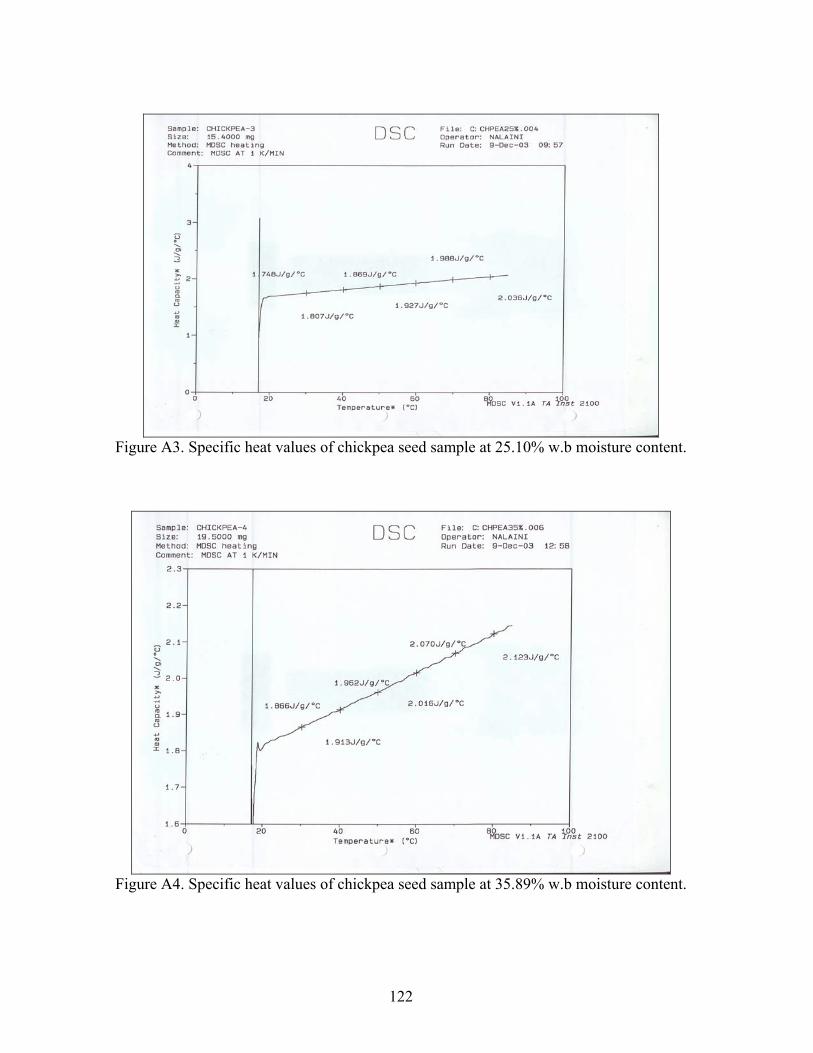
122

Figure A3. Specific heat values of chickpea seed sample at 25.10% w.b moisture content.

Figure A4. Specific heat values of chickpea seed sample at 35.89% w.b moisture content.

123

Figure A5. Specific heat values of chickpea seed sample at 55.97% w.b moisture content.

Figure A6. Specific heat values of chickpea seed sample at 65.24% w.b moisture content.

124

APPENDIX B

Simulation programs used to predict the heat and mass transfer during cooking of

chickpea. Program 1: Program used for simulating the soaked chickpea when cooked at 70°C :HEAT AND MASS TRANSFER DURING COOKING OF CHICKPEA(h70sk.sim) :Temperature and moisture distribution for 70 degree soaked seeds :DM=Moisture diffusivity, m^2/s :ALPHA=Thermal diffusivity, m^2/s :H=Heat transfer coefficient, W/m^2.K :K= Thermal conductivity of chickpea, W/mK :M*=Moisture concentration, db :MS=Moisture concentration at product surface, db :T*= Temperature, C :TA=Ambient temperature, C :TS=Surface temperature, C :INITIAL CONDITIONS CONSTANT ALPHA=2.24E-7, K=0.2632, H=212 CONSTANT DM=8.53E-11 CONSTANT MS=0.01, DR=0.005,T0=24.84,M0=1 CONSTANT TFIN=250, CINT=0.125, TA=69.20 1 SIM;INTERACT;RESET;GOTO 1 INITIAL T1=24.84 T2=24.84 T3=24.84 T4=24.84 T5=24.84 T6=24.84 T7=24.84 T8=24.84 T9=24.84 T10=24.84 TS=24.84 M1=1 M2=1 M3=1 M4=1

125

M5=1 M6=1 M7=1 M8=1 M9=1 M10=1 DYNAMIC ADR2=100*ALPHA/(DR*DR) DDR2=100*DM/(DR*DR) T0'=3*ADR2*(T1-T0) T1'=ADR2*(3*T2-2*T1-T0) T2'=ADR2*(1.6667*T3-2*T2+0.3333*T1) T3'=ADR2*(1.4000*T4-2*T3+0.6000*T2) T4'=ADR2*(1.2857*T5-2*T4+0.7143*T3) T5'=ADR2*(1.2222*T6-2*T5+0.7778*T4) T6'=ADR2*(1.1818*T7-2*T6+0.8182*T5) T7'=ADR2*(1.1538*T8-2*T7+0.8462*T6) T8'=ADR2*(1.1333*T9-2*T8+0.8667*T7) T9'=ADR2*(1.1176*T10-2*T9+0.8824*T8) T10'=4*ADR2*(40/57*TS-T10+17/57*T9) M0'=3*DDR2*(M1-M0) M1'=DDR2*(3*M2-2*M1-M0) M2'=DDR2*(1.6667*M3-2*M2+0.3333*M1) M3'=DDR2*(1.4000*M4-2*M3+0.6000*M2) M4'=DDR2*(1.2857*M5-2*M4+0.7143*M3) M5'=DDR2*(1.2222*M6-2*M5+0.7778*M4) M6'=DDR2*(1.1818*M7-2*M6+0.8182*M5) M7'=DDR2*(1.1538*M8-2*M7+0.8462*M6) M8'=DDR2*(1.1333*M9-2*M8+0.8667*M7) M9'=DDR2*(1.1176*M10-2*M9+0.8824*M8) M10'=4*DDR2*(40/57*MS-M10+17/57*M9) MAVE=(M0+M1+M2+M3+M4+M5+M6+M7+M8+M9+M10)/10 TS=(0.5*DR*H/K*TA+T10)/(1+0.5*DR*H/K) PLOT T,TS,0,TFIN,0,100 OUTPUT T,T0,T1,TS,M1,M2,MAVE PREPARE T,T0,T1,TS,M1,M2,MAVE

126

Program 2: Program used for simulating the unsoaked chickpea when cooked at 70°C :HEAT AND MASS TRANSFER DURING COOKING OF CHICKPEA(h70unsk.sim) :Temperature and moisture distribution for 70 degree unsoaked seeds :DM=Moisture diffusivity, m^2/s :ALPHA=Thermal diffusivity, m^2/s :H=Heat transfer coefficient, W/m^2.K :K= Thermal conductivity of chickpea, W/mK :M*=Moisture concentration, db :MS=Moisture concentration at product surface, db :T*= Temperature, C :TA=Ambient temperature, C :TS=Surface temperature, C :INITIAL CONDITIONS CONSTANT ALPHA=7.36E-8, K=0.1886, H=212 CONSTANT DM=4.13E-11 CONSTANT MS=0.01, DR=0.005,T0=24.84,M0=1 CONSTANT TFIN=250, CINT=0.125, TA=69.20 1 SIM;INTERACT;RESET;GOTO 1 INITIAL T1=24.84 T2=24.84 T3=24.84 T4=24.84 T5=24.84 T6=24.84 T7=24.84 T8=24.84 T9=24.84 T10=24.84 TS=24.84 M1=1 M2=1 M3=1 M4=1 M5=1 M6=1 M7=1 M8=1 M9=1 M10=1

127

DYNAMIC ADR2=100*ALPHA/(DR*DR) DDR2=100*DM/(DR*DR) T0'=3*ADR2*(T1-T0) T1'=ADR2*(3*T2-2*T1-T0) T2'=ADR2*(1.6667*T3-2*T2+0.3333*T1) T3'=ADR2*(1.4000*T4-2*T3+0.6000*T2) T4'=ADR2*(1.2857*T5-2*T4+0.7143*T3) T5'=ADR2*(1.2222*T6-2*T5+0.7778*T4) T6'=ADR2*(1.1818*T7-2*T6+0.8182*T5) T7'=ADR2*(1.1538*T8-2*T7+0.8462*T6) T8'=ADR2*(1.1333*T9-2*T8+0.8667*T7) T9'=ADR2*(1.1176*T10-2*T9+0.8824*T8) T10'=4*ADR2*(40/57*TS-T10+17/57*T9) M0'=3*DDR2*(M1-M0) M1'=DDR2*(3*M2-2*M1-M0) M2'=DDR2*(1.6667*M3-2*M2+0.3333*M1) M3'=DDR2*(1.4000*M4-2*M3+0.6000*M2) M4'=DDR2*(1.2857*M5-2*M4+0.7143*M3) M5'=DDR2*(1.2222*M6-2*M5+0.7778*M4) M6'=DDR2*(1.1818*M7-2*M6+0.8182*M5) M7'=DDR2*(1.1538*M8-2*M7+0.8462*M6) M8'=DDR2*(1.1333*M9-2*M8+0.8667*M7) M9'=DDR2*(1.1176*M10-2*M9+0.8824*M8) M10'=4*DDR2*(40/57*MS-M10+17/57*M9) MAVE=(M0+M1+M2+M3+M4+M5+M6+M7+M8+M9+M10)/10 TS=(0.5*DR*H/K*TA+T10)/(1+0.5*DR*H/K) PLOT T,TS,0,TFIN,0,100 OUTPUT T,T0,T1,TS,M1,M2,MAVE PREPARE T,T0,T1,TS,M1,M2,MAVE

128

APPENDIX C

Simulated Temperature History

Table C1. Temperature distribution of soaked chickpea at 70°C.

Time Temperature (°C) (s) T0 T1 T2 T3 T4 T5 T6 T7 T8 T9 T10 TS

0.000 24.84 24.84 24.84 24.84 24.84 24.84 24.84 24.84 24.84 24.84 24.84 55.34 0.125 24.84 24.84 24.84 24.84 24.84 24.84 24.84 24.84 24.84 24.84 25.09 56.59 0.250 24.84 24.84 24.84 24.84 24.84 24.84 24.84 24.84 24.87 25.51 35.60 61.94 0.375 24.84 24.84 24.84 24.84 24.84 24.84 24.84 24.85 25.02 27.03 42.65 65.36 0.500 24.84 24.84 24.84 24.84 24.84 24.84 24.84 24.89 25.35 28.91 47.35 65.87 0.625 24.84 24.84 24.84 24.84 24.84 24.84 24.85 24.97 25.83 30.88 50.59 66.26 0.750 24.84 24.84 24.84 24.84 24.84 24.84 24.87 25.09 26.45 32.81 52.87 66.58 0.875 24.84 24.84 24.84 24.84 24.84 24.85 24.91 25.28 27.17 34.63 54.54 66.85 1.000 24.84 24.84 24.84 24.84 24.84 24.86 24.96 25.51 27.97 36.31 55.79 67.21 2.375 24.85 24.86 24.87 24.93 25.12 25.67 27.11 30.44 37.01 47.63 61.14 67.48 6.250 27.05 27.56 27.96 29.13 31.14 34.20 38.47 43.98 50.52 57.61 64.56 67.59 7.625 29.30 29.99 30.50 31.95 34.30 37.63 41.96 47.20 53.09 59.22 65.07 67.71 9.000 32.08 32.87 33.42 35.01 37.48 40.83 45.01 49.86 55.12 60.45 65.46 67.71

10.375 35.10 35.93 36.48 38.08 40.53 43.77 47.67 52.09 56.78 61.44 65.78 67.71 11.875 38.42 39.24 39.77 41.31 43.64 46.64 50.21 54.16 58.28 62.32 66.05 67.71 14.375 43.62 44.35 44.82 46.17 48.18 50.73 53.71 56.94 60.26 63.47 66.41 67.71 16.875 48.13 48.74 49.14 50.27 51.94 54.06 56.49 59.11 61.78 64.35 66.68 67.71 18.125 50.10 50.66 51.02 52.04 53.56 55.47 57.66 60.02 62.41 64.71 66.79 67.71 24.375 57.46 57.80 58.01 58.62 59.51 60.64 61.92 63.29 64.67 65.99 67.19 67.71 30.750 61.85 62.04 62.16 62.51 63.03 63.67 64.41 65.19 65.98 66.73 67.41 67.71 36.875 64.29 64.40 64.47 64.68 64.98 65.36 65.78 66.24 66.70 67.14 67.54 67.71 43.125 65.74 65.80 65.84 65.96 66.14 66.35 66.60 66.86 67.13 67.38 67.61 67.71 49.375 66.57 66.61 66.64 66.70 66.80 66.93 67.07 67.22 67.38 67.52 67.66 67.71 55.625 67.06 67.08 67.09 67.13 67.19 67.26 67.34 67.43 67.52 67.61 67.68 67.71 61.875 67.34 67.35 67.36 67.38 67.41 67.45 67.50 67.55 67.60 67.65 67.70 67.71 68.125 67.50 67.50 67.51 67.52 67.54 67.56 67.59 67.62 67.65 67.68 67.70 67.71 74.375 67.59 67.59 67.60 67.60 67.61 67.63 67.64 67.66 67.68 67.69 67.71 67.71 80.625 67.64 67.64 67.65 67.65 67.66 67.66 67.67 67.68 67.69 67.70 67.71 67.71 86.875 67.67 67.67 67.68 67.68 67.68 67.69 67.69 67.70 67.70 67.71 67.71 67.71 99.375 67.70 67.70 67.70 67.70 67.70 67.71 67.71 67.71 67.71 67.71 67.71 67.71 105.620 67.71 67.71 67.71 67.71 67.71 67.71 67.71 67.71 67.71 67.71 67.71 67.71 111.870 67.71 67.71 67.71 67.71 67.71 67.71 67.71 67.71 67.71 67.71 67.71 67.71 118.120 67.71 67.71 67.71 67.71 67.71 67.71 67.71 67.71 67.71 67.71 67.71 67.71 124.380 67.71 67.71 67.71 67.71 67.71 67.71 67.71 67.71 67.71 67.71 67.71 67.71 130.630 67.71 67.71 67.71 67.71 67.71 67.71 67.71 67.71 67.71 67.71 67.71 67.71 136.880 67.71 67.71 67.71 67.71 67.71 67.71 67.71 67.71 67.71 67.71 67.71 67.71 143.130 67.71 67.71 67.71 67.71 67.71 67.71 67.71 67.71 67.71 67.71 67.71 67.71 149.370 67.71 67.71 67.71 67.71 67.71 67.71 67.71 67.71 67.71 67.71 67.71 67.71 155.630 67.71 67.71 67.71 67.71 67.71 67.71 67.71 67.71 67.71 67.71 67.71 67.71 161.880 67.71 67.71 67.71 67.71 67.71 67.71 67.71 67.71 67.71 67.71 67.71 67.71 168.130 67.71 67.71 67.71 67.71 67.71 67.71 67.71 67.71 67.71 67.71 67.71 67.71 174.380 67.71 67.71 67.71 67.71 67.71 67.71 67.71 67.71 67.71 67.71 67.71 67.71

129

180.620 67.71 67.71 67.71 67.71 67.71 67.71 67.71 67.71 67.71 67.71 67.71 67.71 186.880 67.71 67.71 67.71 67.71 67.71 67.71 67.71 67.71 67.71 67.71 67.71 67.71 193.130 67.71 67.71 67.71 67.71 67.71 67.71 67.71 67.71 67.71 67.71 67.71 67.71 199.380 67.71 67.71 67.71 67.71 67.71 67.71 67.71 67.71 67.71 67.71 67.71 67.71 205.630 67.71 67.71 67.71 67.71 67.71 67.71 67.71 67.71 67.71 67.71 67.71 67.71 211.880 67.71 67.71 67.71 67.71 67.71 67.71 67.71 67.71 67.71 67.71 67.71 67.71 224.380 67.71 67.71 67.71 67.71 67.71 67.71 67.71 67.71 67.71 67.71 67.71 67.71 230.630 67.71 67.71 67.71 67.71 67.71 67.71 67.71 67.71 67.71 67.71 67.71 67.71 236.880 67.71 67.71 67.71 67.71 67.71 67.71 67.71 67.71 67.71 67.71 67.71 67.71 249.380 67.71 67.71 67.71 67.71 67.71 67.71 67.71 67.71 67.71 67.71 67.71 67.71

0

10

20

30

40

50

60

70

80

0 10 20 30 40 50 60Time (s)

Tem

pera

ture

(o C)

T0 T1 T2T3 T4 T5T6 T7 T8T9 T10

Figure C1. Simulated cooking curve for soaked kabuli chickpea at 70°C.

Table C2. Temperature distribution of unsoaked chickpea at 70°C.

Time Temperature (°C) (s) T0 T1 T2 T3 T4 T5 T6 T7 T8 T9 T10 TS

0.000 24.84 24.84 24.84 24.84 24.84 24.84 24.84 24.84 24.84 24.84 24.84 53.62 0.125 24.84 24.84 24.84 24.84 24.84 24.84 24.84 24.84 24.84 24.84 24.93 55.97 0.250 24.84 24.84 24.84 24.84 24.84 24.84 24.84 24.84 24.84 24.93 29.11 57.92 0.375 24.84 24.84 24.84 24.84 24.84 24.84 24.84 24.84 24.85 25.17 32.81 60.41 0.500 24.84 24.84 24.84 24.84 24.84 24.84 24.84 24.84 24.87 25.53 36.02 61.46 0.625 24.84 24.84 24.84 24.84 24.84 24.84 24.84 24.84 24.90 25.98 38.81 62.26 0.750 24.84 24.84 24.84 24.84 24.84 24.84 24.84 24.85 24.95 26.50 41.24 62.89 0.875 24.84 24.84 24.84 24.84 24.84 24.84 24.84 24.85 25.02 27.09 43.37 63.39 1.000 24.84 24.84 24.84 24.84 24.84 24.84 24.84 24.86 25.11 27.71 45.23 63.81 2.375 24.84 24.84 24.84 24.84 24.84 24.85 24.91 25.27 27.16 34.97 55.91 64.15 6.250 24.84 24.85 24.86 24.89 25.02 25.42 26.58 29.51 35.75 47.43 62.50 64.44 7.625 24.86 24.87 24.90 24.99 25.25 25.96 27.70 31.44 38.33 49.90 63.42 64.69

130

9.000 24.89 24.93 24.98 25.16 25.61 26.68 28.98 33.35 40.59 51.85 64.12 64.72 10.375 24.96 25.04 25.13 25.42 26.10 27.55 30.34 35.19 42.56 53.45 64.67 65.27 11.875 25.10 25.24 25.38 25.83 26.78 28.62 31.87 37.07 44.43 54.90 65.17 65.77 14.375 25.54 25.81 26.05 26.78 28.18 30.59 34.41 39.91 47.07 56.84 65.81 66.41 16.875 26.29 26.71 27.05 28.05 29.84 32.68 36.83 42.40 49.23 58.35 66.31 66.91 18.125 26.79 27.27 27.65 28.78 30.73 33.73 37.98 43.53 50.17 59.00 66.52 67.12 24.375 30.25 30.99 31.51 33.03 35.46 38.83 43.13 48.25 53.92 61.48 67.32 67.92 30.750 34.75 35.58 36.13 37.74 40.21 43.46 47.42 51.89 56.65 63.22 67.87 68.47 36.875 39.21 40.01 40.54 42.06 44.35 47.30 50.78 54.63 58.63 64.46 68.26 68.86 43.125 43.46 44.19 44.67 46.03 48.05 50.63 53.62 56.88 60.22 65.44 68.56 69.16 49.375 47.25 47.89 48.30 49.48 51.22 53.43 55.97 58.71 61.51 66.22 68.81 69.41 55.625 50.52 51.07 51.42 52.43 53.91 55.78 57.92 60.22 62.55 66.85 69.00 69.60 61.875 53.31 53.77 54.07 54.92 56.17 57.74 59.54 61.47 63.42 67.38 69.16 69.76 68.125 55.66 56.05 56.30 57.02 58.07 59.39 60.90 62.51 64.13 67.81 69.30 69.89 74.375 57.64 57.97 58.18 58.78 59.66 60.76 62.02 63.37 64.72 68.17 69.41 69.97 80.625 59.30 59.57 59.75 60.25 60.99 61.91 62.96 64.09 65.22 68.46 69.50 69.97 86.875 60.69 60.92 61.06 61.48 62.10 62.87 63.75 64.69 65.63 68.71 69.58 69.97 99.375 62.81 62.97 63.08 63.37 63.80 64.34 64.95 65.60 66.26 69.09 69.70 69.97 105.620 63.62 63.76 63.84 64.09 64.45 64.89 65.41 65.95 66.50 69.24 69.74 69.97 111.870 64.30 64.41 64.48 64.69 64.99 65.36 65.79 66.24 66.70 69.36 69.78 69.97 118.120 64.86 64.96 65.02 65.19 65.44 65.75 66.11 66.49 66.87 69.46 69.81 69.97 124.380 65.33 65.41 65.46 65.60 65.81 66.07 66.37 66.69 67.01 69.54 69.83 69.97 130.630 65.73 65.79 65.83 65.95 66.13 66.34 66.59 66.86 67.13 69.61 69.86 69.97 136.880 66.05 66.11 66.14 66.24 66.39 66.57 66.78 67.00 67.22 69.67 69.87 69.97 143.130 66.33 66.37 66.40 66.49 66.61 66.76 66.93 67.12 67.30 69.72 69.89 69.97 149.370 66.56 66.60 66.62 66.69 66.79 66.92 67.06 67.22 67.37 69.76 69.90 69.97 155.630 66.75 66.78 66.80 66.86 66.94 67.05 67.17 67.30 67.43 69.79 69.91 69.97 161.880 66.91 66.93 66.95 67.00 67.07 67.16 67.26 67.37 67.48 69.82 69.92 69.97 168.130 67.04 67.06 67.08 67.12 67.18 67.25 67.33 67.42 67.52 69.85 69.93 69.97 174.380 67.15 67.17 67.18 67.22 67.27 67.33 67.40 67.47 67.55 69.87 69.93 69.97 180.620 67.25 67.26 67.27 67.30 67.34 67.39 67.45 67.51 67.58 69.88 69.94 69.97 186.880 67.32 67.34 67.34 67.37 67.40 67.44 67.49 67.55 67.60 69.90 69.94 69.97 193.130 67.39 67.40 67.40 67.42 67.45 67.49 67.53 67.57 67.62 69.91 69.95 69.97 199.380 67.44 67.45 67.46 67.47 67.50 67.53 67.56 67.60 67.63 69.92 69.95 69.97 205.630 67.49 67.49 67.50 67.51 67.53 67.56 67.59 67.62 67.65 69.93 69.95 69.97 211.880 67.52 67.53 67.53 67.55 67.56 67.58 67.61 67.63 67.66 69.93 69.96 69.97 224.380 67.58 67.59 67.59 67.60 67.61 67.62 67.64 67.66 67.68 69.94 69.96 69.97 230.630 67.60 67.61 67.61 67.62 67.63 67.64 67.65 67.67 67.68 69.95 69.96 69.97 236.880 67.62 67.63 67.63 67.63 67.64 67.65 67.66 67.67 67.69 69.95 69.96 69.97 249.380 67.65 67.65 67.65 67.66 67.66 67.67 67.68 67.69 67.70 69.95 69.96 69.97

131

0

10

20

30

40

50

60

70

80

0 50 100 150Time (s)

Tem

pera

ture

(o C)

T0 T1 T2 T3T4 T5 T6 T7T8 T9 T10

Figure C2. Simulated cooking curve for unsoaked kabuli chickpea at 70°C.

Table C3. Temperature distribution of soaked chickpea at 80°C.

Time Temperature (°C)

(s) T0 T1 T2 T3 T4 T5 T6 T7 T8 T9 T10 TS 0.000 20.61 20.61 20.61 20.61 20.61 20.61 20.61 20.61 20.61 20.61 20.61 59.27 0.125 20.61 20.61 20.61 20.61 20.61 20.61 20.61 20.61 20.61 20.61 21.03 62.21 0.250 20.61 20.61 20.61 20.61 20.61 20.61 20.61 20.61 20.67 21.80 37.64 64.29 0.375 20.61 20.61 20.61 20.61 20.61 20.61 20.61 20.64 20.96 24.38 48.06 65.85 0.500 20.61 20.61 20.61 20.61 20.61 20.61 20.62 20.71 21.56 27.45 54.63 72.47 0.625 20.61 20.61 20.61 20.61 20.61 20.61 20.64 20.87 22.43 30.58 58.93 76.75 0.750 20.61 20.61 20.61 20.61 20.61 20.62 20.68 21.12 23.51 33.54 61.87 77.39 0.875 20.61 20.61 20.61 20.61 20.61 20.63 20.76 21.47 24.73 36.26 63.95 77.88 1.000 20.61 20.61 20.61 20.61 20.62 20.66 20.87 21.91 26.05 38.73 65.51 78.27 2.375 20.63 20.66 20.70 20.83 21.23 22.27 24.79 30.12 39.80 54.43 72.13 78.61 6.250 25.25 26.12 26.76 28.64 31.75 36.27 42.33 49.85 58.49 67.62 76.41 79.06 7.625 29.30 30.38 31.13 33.30 36.72 41.42 47.35 54.31 61.94 69.72 77.05 79.39 9.000 33.94 35.09 35.87 38.11 41.55 46.11 51.66 57.95 64.65 71.34 77.54 79.52

10.375 38.70 39.84 40.60 42.77 46.05 50.31 55.36 60.98 66.85 72.62 77.93 79.79 11.875 43.71 44.78 45.48 47.49 50.49 54.34 58.83 63.75 68.83 73.76 78.27 80.05 14.375 51.15 52.06 52.64 54.32 56.80 59.93 63.54 67.44 71.41 75.24 78.72 80.18 16.875 57.30 58.03 58.50 59.85 61.83 64.33 67.19 70.26 73.37 76.35 79.05 80.20 18.125 59.90 60.55 60.97 62.17 63.94 66.16 68.70 71.42 74.17 76.80 79.18 80.20 24.375 69.18 69.54 69.77 70.43 71.40 72.61 73.99 75.46 76.95 78.37 79.65 80.20 30.750 74.31 74.50 74.63 74.98 75.50 76.15 76.88 77.67 78.46 79.22 79.91 80.20 36.875 76.98 77.08 77.15 77.34 77.63 77.98 78.38 78.82 79.25 79.66 80.04 80.20 43.125 78.46 78.51 78.55 78.65 78.81 79.00 79.22 79.45 79.69 79.91 80.11 80.20 49.375 79.26 79.29 79.31 79.36 79.45 79.55 79.67 79.80 79.92 80.04 80.15 80.20 55.625 79.69 79.71 79.72 79.75 79.79 79.85 79.91 79.98 80.05 80.12 80.17 80.20

132

61.875 79.92 79.93 79.94 79.96 79.98 80.01 80.04 80.08 80.12 80.15 80.19 80.20 68.125 80.05 80.06 80.06 80.07 80.08 80.10 80.12 80.14 80.16 80.18 80.19 80.20 74.375 80.12 80.12 80.12 80.13 80.14 80.14 80.15 80.17 80.18 80.19 80.20 80.20 80.625 80.16 80.16 80.16 80.16 80.17 80.17 80.18 80.18 80.19 80.19 80.20 80.20 86.875 80.18 80.18 80.18 80.18 80.18 80.18 80.19 80.19 80.19 80.20 80.20 80.20 99.375 80.19 80.19 80.19 80.19 80.19 80.20 80.20 80.20 80.20 80.20 80.20 80.20 105.620 80.20 80.20 80.20 80.20 80.20 80.20 80.20 80.20 80.20 80.20 80.20 80.20 111.870 80.20 80.20 80.20 80.20 80.20 80.20 80.20 80.20 80.20 80.20 80.20 80.20 118.120 80.20 80.20 80.20 80.20 80.20 80.20 80.20 80.20 80.20 80.20 80.20 80.20 124.380 80.20 80.20 80.20 80.20 80.20 80.20 80.20 80.20 80.20 80.20 80.20 80.20 130.630 80.20 80.20 80.20 80.20 80.20 80.20 80.20 80.20 80.20 80.20 80.20 80.20 136.880 80.20 80.20 80.20 80.20 80.20 80.20 80.20 80.20 80.20 80.20 80.20 80.20 143.130 80.20 80.20 80.20 80.20 80.20 80.20 80.20 80.20 80.20 80.20 80.20 80.20 149.370 80.20 80.20 80.20 80.20 80.20 80.20 80.20 80.20 80.20 80.20 80.20 80.20 155.630 80.20 80.20 80.20 80.20 80.20 80.20 80.20 80.20 80.20 80.20 80.20 80.20 161.880 80.20 80.20 80.20 80.20 80.20 80.20 80.20 80.20 80.20 80.20 80.20 80.20 168.130 80.20 80.20 80.20 80.20 80.20 80.20 80.20 80.20 80.20 80.20 80.20 80.20 174.380 80.20 80.20 80.20 80.20 80.20 80.20 80.20 80.20 80.20 80.20 80.20 80.20 180.620 80.20 80.20 80.20 80.20 80.20 80.20 80.20 80.20 80.20 80.20 80.20 80.20 186.880 80.20 80.20 80.20 80.20 80.20 80.20 80.20 80.20 80.20 80.20 80.20 80.20 193.130 80.20 80.20 80.20 80.20 80.20 80.20 80.20 80.20 80.20 80.20 80.20 80.20 199.380 80.20 80.20 80.20 80.20 80.20 80.20 80.20 80.20 80.20 80.20 80.20 80.20 205.630 80.20 80.20 80.20 80.20 80.20 80.20 80.20 80.20 80.20 80.20 80.20 80.20 211.880 80.20 80.20 80.20 80.20 80.20 80.20 80.20 80.20 80.20 80.20 80.20 80.20 224.380 80.20 80.20 80.20 80.20 80.20 80.20 80.20 80.20 80.20 80.20 80.20 80.20 230.630 80.20 80.20 80.20 80.20 80.20 80.20 80.20 80.20 80.20 80.20 80.20 80.20 236.880 80.20 80.20 80.20 80.20 80.20 80.20 80.20 80.20 80.20 80.20 80.20 80.20 249.380 80.20 80.20 80.20 80.20 80.20 80.20 80.20 80.20 80.20 80.20 80.20 80.20

0102030405060708090

0 10 20 30 40 50Time (s)

Tem

pera

ture

(o C)

T0 T1 T2 T3T4 T5 T6 T7T8 T9 T10

Figure C3. Simulated cooking curve for soaked kabuli chickpea at 80°C.

133

Table C4. Temperature distribution of unsoaked chickpea at 80°C.

Time Temperature (°C) (s) T0 T1 T2 T3 T4 T5 T6 T7 T8 T9 T10 TS

0.000 23.87 23.87 23.87 23.87 23.87 23.87 23.87 23.87 23.87 23.87 23.87 67.23 0.125 23.87 23.87 23.87 23.87 23.87 23.87 23.87 23.87 23.87 23.87 24.08 72.56 0.250 23.87 23.87 23.87 23.87 23.87 23.87 23.87 23.87 23.87 24.11 32.86 73.32 0.375 23.87 23.87 23.87 23.87 23.87 23.87 23.87 23.87 23.90 24.70 39.24 73.91 0.500 23.87 23.87 23.87 23.87 23.87 23.87 23.87 23.87 23.96 25.51 44.18 74.39 0.625 23.87 23.87 23.87 23.87 23.87 23.87 23.87 23.88 24.06 26.47 48.14 74.83 0.750 23.87 23.87 23.87 23.87 23.87 23.87 23.87 23.89 24.20 27.53 51.38 75.42 0.875 23.87 23.87 23.87 23.87 23.87 23.87 23.87 23.91 24.38 28.65 54.06 75.90 1.000 23.87 23.87 23.87 23.87 23.87 23.87 23.88 23.94 24.60 29.79 56.28 76.11 2.375 23.87 23.87 23.87 23.87 23.88 23.91 24.10 25.04 28.93 41.07 66.88 76.92 6.250 23.90 23.92 23.96 24.10 24.50 25.54 28.01 33.17 42.39 56.05 72.21 77.50 7.625 23.97 24.04 24.13 24.43 25.17 26.82 30.18 36.27 45.86 58.71 72.97 77.91 9.000 24.14 24.29 24.45 24.97 26.11 28.37 32.47 39.15 48.77 60.79 73.56 78.23

10.375 24.45 24.71 24.96 25.73 27.28 30.09 34.76 41.79 51.25 62.47 74.04 78.48 11.875 24.99 25.39 25.74 26.79 28.77 32.08 37.20 44.40 53.56 64.00 74.48 78.68 14.375 26.42 27.06 27.56 29.03 31.58 35.49 41.02 48.20 56.75 66.02 75.07 78.83 16.875 28.46 29.28 29.90 31.68 34.62 38.86 44.49 51.43 59.33 67.62 75.55 78.96 18.125 29.66 30.56 31.21 33.11 36.17 40.49 46.10 52.87 60.45 68.30 75.76 79.06 24.375 36.67 37.75 38.47 40.55 43.73 47.93 53.02 58.77 64.87 70.94 76.57 79.10 30.750 44.12 45.13 45.79 47.69 50.54 54.20 58.49 63.19 68.06 72.80 77.15 79.10 36.875 50.54 51.42 51.99 53.62 56.03 59.08 62.62 66.44 70.35 74.12 77.56 79.10 43.125 56.09 56.82 57.29 58.63 60.61 63.10 65.96 69.04 72.16 75.16 77.88 79.10 49.375 60.65 61.25 61.62 62.71 64.31 66.32 68.62 71.09 73.58 75.97 78.13 79.10 55.625 64.34 64.82 65.12 66.00 67.29 68.90 70.74 72.71 74.70 76.60 78.33 79.10 61.875 67.31 67.69 67.93 68.64 69.67 70.96 72.43 74.01 75.59 77.11 78.48 79.10 68.125 69.68 69.99 70.18 70.75 71.57 72.60 73.78 75.04 76.30 77.51 78.61 79.10 74.375 71.58 71.83 71.98 72.43 73.09 73.91 74.85 75.86 76.87 77.83 78.71 79.10 80.625 73.10 73.29 73.42 73.78 74.30 74.96 75.71 76.51 77.32 78.09 78.79 79.10 86.875 74.31 74.47 74.57 74.85 75.27 75.80 76.40 77.04 77.68 78.29 78.85 79.10 99.375 76.05 76.15 76.21 76.39 76.66 77.00 77.38 77.79 78.20 78.59 78.94 79.10 105.620 76.67 76.75 76.80 76.94 77.15 77.42 77.73 78.05 78.38 78.69 78.97 79.10 111.870 77.16 77.22 77.26 77.38 77.55 77.76 78.00 78.26 78.52 78.77 79.00 79.10 118.120 77.55 77.60 77.63 77.73 77.86 78.03 78.23 78.43 78.64 78.84 79.02 79.10 124.380 77.86 77.90 77.93 78.00 78.11 78.25 78.40 78.57 78.73 78.89 79.04 79.10 130.630 78.11 78.15 78.17 78.22 78.31 78.42 78.54 78.67 78.81 78.93 79.05 79.10 136.880 78.31 78.34 78.35 78.40 78.47 78.56 78.66 78.76 78.87 78.97 79.06 79.10 143.130 78.47 78.49 78.51 78.54 78.60 78.67 78.75 78.83 78.91 78.99 79.07 79.10 149.370 78.60 78.61 78.63 78.66 78.70 78.75 78.82 78.88 78.95 79.02 79.07 79.10 155.630 78.70 78.71 78.72 78.75 78.78 78.82 78.87 78.93 78.98 79.03 79.08 79.10 161.880 78.78 78.79 78.80 78.82 78.85 78.88 78.92 78.96 79.01 79.05 79.08 79.10 168.130 78.85 78.85 78.86 78.87 78.90 78.92 78.96 78.99 79.02 79.06 79.09 79.10 174.380 78.90 78.90 78.91 78.92 78.94 78.96 78.99 79.01 79.04 79.07 79.09 79.10 180.620 78.94 78.94 78.95 78.96 78.97 78.99 79.01 79.03 79.05 79.07 79.09 79.10 186.880 78.97 78.98 78.98 78.99 79.00 79.01 79.03 79.04 79.06 79.08 79.09 79.10 193.130 79.00 79.00 79.00 79.01 79.02 79.03 79.04 79.06 79.07 79.08 79.10 79.10 199.380 79.02 79.02 79.02 79.03 79.03 79.04 79.05 79.06 79.08 79.09 79.10 79.10

134

205.630 79.03 79.04 79.04 79.04 79.05 79.06 79.06 79.07 79.08 79.09 79.10 79.10 211.880 79.05 79.05 79.05 79.05 79.06 79.06 79.07 79.08 79.08 79.09 79.10 79.10 224.380 79.07 79.07 79.07 79.07 79.07 79.08 79.08 79.09 79.09 79.09 79.10 79.10 230.630 79.07 79.07 79.08 79.08 79.08 79.08 79.09 79.09 79.09 79.10 79.10 79.10 236.880 79.08 79.08 79.08 79.08 79.08 79.09 79.09 79.09 79.09 79.10 79.10 79.10 249.380 79.09 79.09 79.09 79.09 79.09 79.09 79.09 79.09 79.10 79.10 79.10 79.10

0

10

20

30

40

50

60

70

80

0 10 20 30 40 50 60 70 80 90 100 110 120 130 140Time (s)

Tem

pera

ture

(o C)

T0 T1 T2 T3T4 T5 T6 T7T8 T9 T10

Figure C4. Simulated cooking curve for unsoaked kabuli chickpea at 80°C. Table C5. Temperature distribution of soaked chickpea at 90°C.

Time Temperature (°C) (s) T0 T1 T2 T3 T4 T5 T6 T7 T8 T9 T10 TS

0.000 20.54 20.54 20.54 20.54 20.54 20.54 20.54 20.54 20.54 20.54 20.54 65.98 0.125 20.54 20.54 20.54 20.54 20.54 20.54 20.54 20.54 20.54 20.54 21.06 69.27 0.250 20.54 20.54 20.54 20.54 20.54 20.54 20.54 20.54 20.61 21.98 40.95 71.61 0.375 20.54 20.54 20.54 20.54 20.54 20.54 20.54 20.57 20.97 25.05 52.90 73.36 0.500 20.54 20.54 20.54 20.54 20.54 20.54 20.55 20.66 21.68 28.65 60.33 80.74 0.625 20.54 20.54 20.54 20.54 20.54 20.54 20.58 20.85 22.71 32.28 65.18 85.49 0.750 20.54 20.54 20.54 20.54 20.54 20.55 20.63 21.15 23.97 35.71 68.47 85.86 0.875 20.54 20.54 20.54 20.54 20.54 20.57 20.72 21.56 25.41 38.86 70.81 86.42 1.000 20.54 20.54 20.54 20.54 20.55 20.59 20.85 22.08 26.94 41.70 72.56 86.86 2.375 20.57 20.60 20.64 20.81 21.27 22.50 25.44 31.63 42.83 59.66 79.94 87.26 6.250 25.98 26.99 27.74 29.91 33.51 38.73 45.70 54.34 64.23 74.67 84.69 87.35 7.625 30.70 31.94 32.80 35.31 39.25 44.66 51.46 59.44 68.17 77.05 85.41 87.74 9.000 36.06 37.39 38.28 40.86 44.81 50.05 56.40 63.60 71.26 78.89 85.97 87.91

10.375 41.56 42.87 43.74 46.23 49.99 54.86 60.65 67.07 73.77 80.36 86.41 88.47 11.875 47.32 48.55 49.35 51.65 55.09 59.48 64.62 70.24 76.03 81.66 86.81 88.78 14.375 55.87 56.91 57.57 59.49 62.31 65.89 70.01 74.46 78.99 83.36 87.32 88.94 16.875 62.91 63.75 64.28 65.82 68.08 70.93 74.19 77.69 81.23 84.63 87.71 89.03 18.125 65.89 66.64 67.11 68.48 70.50 73.03 75.92 79.02 82.15 85.16 87.88 89.07 24.375 76.49 76.91 77.17 77.92 79.02 80.40 81.98 83.66 85.35 86.97 88.44 89.10

135

30.750 82.36 82.58 82.72 83.12 83.71 84.45 85.29 86.19 87.10 87.96 88.75 89.10 36.875 85.41 85.53 85.61 85.83 86.15 86.55 87.02 87.51 88.00 88.48 88.91 89.10 43.125 87.10 87.17 87.21 87.33 87.50 87.72 87.97 88.24 88.51 88.76 89.00 89.10 49.375 88.02 88.05 88.08 88.14 88.24 88.35 88.49 88.63 88.78 88.92 89.04 89.10 55.625 88.52 88.53 88.55 88.58 88.63 88.70 88.77 88.85 88.93 89.00 89.07 89.10 61.875 88.78 88.79 88.80 88.82 88.85 88.88 88.92 88.96 89.01 89.05 89.08 89.10 68.125 88.93 88.93 88.94 88.95 88.96 88.98 89.00 89.03 89.05 89.07 89.09 89.10 74.375 89.01 89.01 89.01 89.02 89.03 89.04 89.05 89.06 89.07 89.08 89.10 89.10 80.625 89.05 89.05 89.05 89.06 89.06 89.07 89.07 89.08 89.09 89.09 89.10 89.10 86.875 89.07 89.07 89.07 89.08 89.08 89.08 89.09 89.09 89.09 89.10 89.10 89.10 99.375 89.09 89.09 89.09 89.09 89.09 89.10 89.10 89.10 89.10 89.10 89.10 89.10

105.620 89.10 89.10 89.10 89.10 89.10 89.10 89.10 89.10 89.10 89.10 89.10 89.10 111.870 89.10 89.10 89.10 89.10 89.10 89.10 89.10 89.10 89.10 89.10 89.10 89.10 118.120 89.10 89.10 89.10 89.10 89.10 89.10 89.10 89.10 89.10 89.10 89.10 89.10 124.380 89.10 89.10 89.10 89.10 89.10 89.10 89.10 89.10 89.10 89.10 89.10 89.10 130.630 89.10 89.10 89.10 89.10 89.10 89.10 89.10 89.10 89.10 89.10 89.10 89.10 136.880 89.10 89.10 89.10 89.10 89.10 89.10 89.10 89.10 89.10 89.10 89.10 89.10 143.130 89.10 89.10 89.10 89.10 89.10 89.10 89.10 89.10 89.10 89.10 89.10 89.10 149.370 89.10 89.10 89.10 89.10 89.10 89.10 89.10 89.10 89.10 89.10 89.10 89.10 155.630 89.10 89.10 89.10 89.10 89.10 89.10 89.10 89.10 89.10 89.10 89.10 89.10 161.880 89.10 89.10 89.10 89.10 89.10 89.10 89.10 89.10 89.10 89.10 89.10 89.10 168.130 89.10 89.10 89.10 89.10 89.10 89.10 89.10 89.10 89.10 89.10 89.10 89.10 174.380 89.10 89.10 89.10 89.10 89.10 89.10 89.10 89.10 89.10 89.10 89.10 89.10 180.620 89.10 89.10 89.10 89.10 89.10 89.10 89.10 89.10 89.10 89.10 89.10 89.10 186.880 89.10 89.10 89.10 89.10 89.10 89.10 89.10 89.10 89.10 89.10 89.10 89.10 193.130 89.10 89.10 89.10 89.10 89.10 89.10 89.10 89.10 89.10 89.10 89.10 89.10 199.380 89.10 89.10 89.10 89.10 89.10 89.10 89.10 89.10 89.10 89.10 89.10 89.10 205.630 89.10 89.10 89.10 89.10 89.10 89.10 89.10 89.10 89.10 89.10 89.10 89.10 211.880 89.10 89.10 89.10 89.10 89.10 89.10 89.10 89.10 89.10 89.10 89.10 89.10 224.380 89.10 89.10 89.10 89.10 89.10 89.10 89.10 89.10 89.10 89.10 89.10 89.10 230.630 89.10 89.10 89.10 89.10 89.10 89.10 89.10 89.10 89.10 89.10 89.10 89.10 236.880 89.10 89.10 89.10 89.10 89.10 89.10 89.10 89.10 89.10 89.10 89.10 89.10 249.380 89.10 89.10 89.10 89.10 89.10 89.10 89.10 89.10 89.10 89.10 89.10 89.10

0102030405060708090

100

0 10 20 30 40 50 60Time (s)

Tem

pera

ture

(o C)

T0 T1 T2 T3T4 T5 T6 T7T8 T9 T10

Figure C5. Simulated cooking curve for soaked kabuli chickpea at 90°C.

136

Table C6. Temperature distribution of unsoaked chickpea at 90°C.

Time Temperature (°C) (s) T0 T1 T2 T3 T4 T5 T6 T7 T8 T9 T10 TS

0.000 26.51 26.51 26.51 26.51 26.51 26.51 26.51 26.51 26.51 26.51 26.51 62.74 0.125 26.51 26.51 26.51 26.51 26.51 26.51 26.51 26.51 26.51 26.51 27.43 65.72 0.250 26.51 26.51 26.51 26.51 26.51 26.51 26.51 26.51 26.52 27.10 44.07 67.96 0.375 26.51 26.51 26.51 26.51 26.51 26.51 26.51 26.51 26.58 28.23 52.35 69.67 0.500 26.51 26.51 26.51 26.51 26.51 26.51 26.51 26.52 26.71 29.62 57.97 76.55 0.625 26.51 26.51 26.51 26.51 26.51 26.51 26.51 26.53 26.90 31.14 62.00 82.39 0.750 26.51 26.51 26.51 26.51 26.51 26.51 26.51 26.56 27.16 32.70 64.98 83.42 0.875 26.51 26.51 26.51 26.51 26.51 26.51 26.52 26.60 27.48 34.27 67.22 84.22 1.000 26.51 26.51 26.51 26.51 26.51 26.51 26.52 26.66 27.86 35.81 68.93 84.86 2.375 26.51 26.51 26.51 26.51 26.52 26.59 26.93 28.46 33.93 48.78 76.10 85.44 6.250 26.57 26.63 26.70 26.95 27.59 29.15 32.51 38.96 49.66 64.66 81.94 86.20 7.625 26.72 26.86 27.02 27.51 28.63 30.94 35.30 42.65 53.59 67.64 82.97 86.78 9.000 27.05 27.31 27.57 28.36 29.99 33.02 38.15 46.05 56.89 70.00 83.77 87.03

10.375 27.61 28.02 28.39 29.51 31.63 35.27 40.97 49.13 59.70 71.93 84.41 87.98 11.875 28.52 29.11 29.60 31.05 33.65 37.81 43.92 52.17 62.34 73.68 84.99 88.41 14.375 30.74 31.60 32.25 34.16 37.35 42.07 48.49 56.58 65.98 76.01 85.75 88.87 16.875 33.67 34.73 35.49 37.69 41.23 46.20 52.61 60.31 68.93 77.84 86.33 89.22 18.125 35.33 36.46 37.25 39.55 43.17 48.17 54.51 61.98 70.20 78.62 86.58 89.49 24.375 44.47 45.70 46.51 48.85 52.40 57.03 62.56 68.73 75.21 81.61 87.53 89.69 30.750 53.53 54.63 55.33 57.38 60.42 64.30 68.81 73.73 78.79 83.70 88.18 89.86 36.875 61.00 61.92 62.50 64.19 66.68 69.83 73.45 77.36 81.33 85.16 88.64 89.80 43.125 67.24 67.97 68.44 69.79 71.78 74.28 77.14 80.20 83.31 86.29 88.99 89.88 49.375 72.21 72.79 73.16 74.23 75.79 77.76 80.00 82.41 84.83 87.15 89.26 89.96 55.625 76.13 76.58 76.87 77.71 78.94 80.48 82.24 84.12 86.01 87.82 89.46 90.02 61.875 79.20 79.56 79.79 80.44 81.41 82.61 83.99 85.45 86.93 88.35 89.63 90.10 68.125 81.61 81.89 82.07 82.58 83.33 84.27 85.35 86.49 87.65 88.75 89.75 90.13 74.375 83.49 83.71 83.85 84.25 84.84 85.57 86.41 87.31 88.21 89.07 89.85 90.15 80.625 84.96 85.13 85.24 85.55 86.01 86.59 87.24 87.94 88.65 89.32 89.93 90.17 86.875 86.11 86.24 86.33 86.57 86.93 87.38 87.89 88.44 88.99 89.51 89.99 90.18 99.375 87.71 87.79 87.84 87.99 88.21 88.48 88.79 89.12 89.46 89.78 90.07 90.19

105.620 88.25 88.32 88.36 88.47 88.64 88.86 89.10 89.36 89.62 89.87 90.10 90.20 111.870 88.68 88.73 88.76 88.85 88.98 89.15 89.34 89.54 89.75 89.94 90.12 90.20 118.120 89.01 89.05 89.08 89.15 89.25 89.38 89.53 89.69 89.85 90.00 90.14 90.20 124.380 89.27 89.30 89.32 89.38 89.46 89.56 89.68 89.80 89.93 90.04 90.15 90.20 130.630 89.48 89.50 89.51 89.56 89.62 89.70 89.79 89.89 89.99 90.08 90.16 90.20 136.880 89.63 89.65 89.67 89.70 89.75 89.81 89.88 89.96 90.03 90.11 90.17 90.20 143.130 89.76 89.77 89.78 89.81 89.85 89.90 89.95 90.01 90.07 90.13 90.18 90.20 149.370 89.86 89.87 89.87 89.89 89.92 89.96 90.01 90.05 90.10 90.14 90.18 90.20 155.630 89.93 89.94 89.95 89.96 89.99 90.01 90.05 90.08 90.12 90.16 90.19 90.20 161.880 89.99 90.00 90.00 90.01 90.03 90.06 90.08 90.11 90.14 90.17 90.19 90.20 168.130 90.04 90.04 90.05 90.05 90.07 90.09 90.11 90.13 90.15 90.17 90.19 90.20 174.380 90.07 90.08 90.08 90.09 90.10 90.11 90.13 90.15 90.16 90.18 90.19 90.20 180.620 90.10 90.10 90.11 90.11 90.12 90.13 90.14 90.16 90.17 90.18 90.20 90.20 186.880 90.12 90.12 90.13 90.13 90.14 90.15 90.16 90.17 90.18 90.19 90.20 90.20 193.130 90.14 90.14 90.14 90.15 90.15 90.16 90.17 90.17 90.18 90.19 90.20 90.20 199.380 90.15 90.15 90.16 90.16 90.16 90.17 90.17 90.18 90.19 90.19 90.20 90.20 205.630 90.16 90.16 90.17 90.17 90.17 90.17 90.18 90.18 90.19 90.19 90.20 90.20 211.880 90.17 90.17 90.17 90.17 90.18 90.18 90.18 90.19 90.19 90.20 90.20 90.20

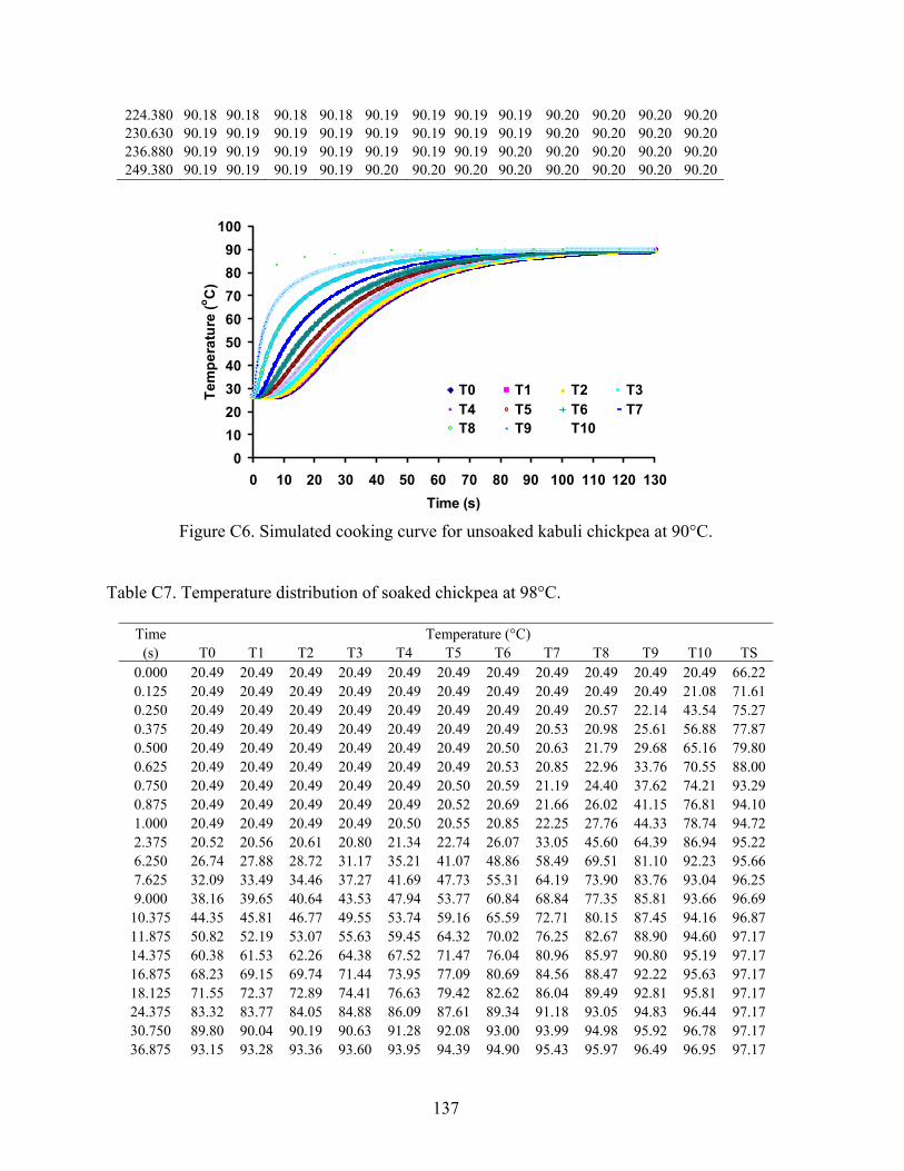
137

224.380 90.18 90.18 90.18 90.18 90.19 90.19 90.19 90.19 90.20 90.20 90.20 90.20 230.630 90.19 90.19 90.19 90.19 90.19 90.19 90.19 90.19 90.20 90.20 90.20 90.20 236.880 90.19 90.19 90.19 90.19 90.19 90.19 90.19 90.20 90.20 90.20 90.20 90.20 249.380 90.19 90.19 90.19 90.19 90.20 90.20 90.20 90.20 90.20 90.20 90.20 90.20

0102030405060708090

100

0 10 20 30 40 50 60 70 80 90 100 110 120 130Time (s)

Tem

pera

ture

(o C)

T0 T1 T2 T3T4 T5 T6 T7T8 T9 T10

Figure C6. Simulated cooking curve for unsoaked kabuli chickpea at 90°C.

Table C7. Temperature distribution of soaked chickpea at 98°C.

Time Temperature (°C) (s) T0 T1 T2 T3 T4 T5 T6 T7 T8 T9 T10 TS

0.000 20.49 20.49 20.49 20.49 20.49 20.49 20.49 20.49 20.49 20.49 20.49 66.22 0.125 20.49 20.49 20.49 20.49 20.49 20.49 20.49 20.49 20.49 20.49 21.08 71.61 0.250 20.49 20.49 20.49 20.49 20.49 20.49 20.49 20.49 20.57 22.14 43.54 75.27 0.375 20.49 20.49 20.49 20.49 20.49 20.49 20.49 20.53 20.98 25.61 56.88 77.87 0.500 20.49 20.49 20.49 20.49 20.49 20.49 20.50 20.63 21.79 29.68 65.16 79.80 0.625 20.49 20.49 20.49 20.49 20.49 20.49 20.53 20.85 22.96 33.76 70.55 88.00 0.750 20.49 20.49 20.49 20.49 20.49 20.50 20.59 21.19 24.40 37.62 74.21 93.29 0.875 20.49 20.49 20.49 20.49 20.49 20.52 20.69 21.66 26.02 41.15 76.81 94.10 1.000 20.49 20.49 20.49 20.49 20.50 20.55 20.85 22.25 27.76 44.33 78.74 94.72 2.375 20.52 20.56 20.61 20.80 21.34 22.74 26.07 33.05 45.60 64.39 86.94 95.22 6.250 26.74 27.88 28.72 31.17 35.21 41.07 48.86 58.49 69.51 81.10 92.23 95.66 7.625 32.09 33.49 34.46 37.27 41.69 47.73 55.31 64.19 73.90 83.76 93.04 96.25 9.000 38.16 39.65 40.64 43.53 47.94 53.77 60.84 68.84 77.35 85.81 93.66 96.69

10.375 44.35 45.81 46.77 49.55 53.74 59.16 65.59 72.71 80.15 87.45 94.16 96.87 11.875 50.82 52.19 53.07 55.63 59.45 64.32 70.02 76.25 82.67 88.90 94.60 97.17 14.375 60.38 61.53 62.26 64.38 67.52 71.47 76.04 80.96 85.97 90.80 95.19 97.17 16.875 68.23 69.15 69.74 71.44 73.95 77.09 80.69 84.56 88.47 92.22 95.63 97.17 18.125 71.55 72.37 72.89 74.41 76.63 79.42 82.62 86.04 89.49 92.81 95.81 97.17 24.375 83.32 83.77 84.05 84.88 86.09 87.61 89.34 91.18 93.05 94.83 96.44 97.17 30.750 89.80 90.04 90.19 90.63 91.28 92.08 93.00 93.99 94.98 95.92 96.78 97.17 36.875 93.15 93.28 93.36 93.60 93.95 94.39 94.90 95.43 95.97 96.49 96.95 97.17

138

43.125 95.00 95.07 95.12 95.25 95.44 95.67 95.94 96.23 96.52 96.80 97.05 97.17 49.375 96.00 96.04 96.06 96.13 96.24 96.36 96.51 96.66 96.82 96.97 97.11 97.17 55.625 96.54 96.56 96.57 96.61 96.67 96.73 96.81 96.90 96.98 97.06 97.13 97.17 61.875 96.83 96.84 96.85 96.87 96.90 96.93 96.98 97.02 97.07 97.11 97.15 97.17 68.125 96.98 96.99 96.99 97.01 97.02 97.04 97.06 97.09 97.11 97.14 97.16 97.17 74.375 97.07 97.07 97.07 97.08 97.09 97.10 97.11 97.12 97.14 97.15 97.16 97.17 80.625 97.11 97.12 97.12 97.12 97.12 97.13 97.14 97.14 97.15 97.16 97.16 97.17 86.875 97.14 97.14 97.14 97.14 97.14 97.15 97.15 97.15 97.16 97.16 97.17 97.17 99.375 97.16 97.16 97.16 97.16 97.16 97.16 97.16 97.16 97.16 97.17 97.17 97.17 105.620 97.16 97.16 97.16 97.16 97.16 97.16 97.16 97.16 97.17 97.17 97.17 97.17 111.870 97.16 97.16 97.16 97.16 97.16 97.16 97.17 97.17 97.17 97.17 97.17 97.17 118.120 97.17 97.17 97.17 97.17 97.17 97.17 97.17 97.17 97.17 97.17 97.17 97.17 124.380 97.17 97.17 97.17 97.17 97.17 97.17 97.17 97.17 97.17 97.17 97.17 97.17 130.630 97.17 97.17 97.17 97.17 97.17 97.17 97.17 97.17 97.17 97.17 97.17 97.17 136.880 97.17 97.17 97.17 97.17 97.17 97.17 97.17 97.17 97.17 97.17 97.17 97.17 143.130 97.17 97.17 97.17 97.17 97.17 97.17 97.17 97.17 97.17 97.17 97.17 97.17 149.370 97.17 97.17 97.17 97.17 97.17 97.17 97.17 97.17 97.17 97.17 97.17 97.17 155.630 97.17 97.17 97.17 97.17 97.17 97.17 97.17 97.17 97.17 97.17 97.17 97.17 161.880 97.17 97.17 97.17 97.17 97.17 97.17 97.17 97.17 97.17 97.17 97.17 97.17 168.130 97.17 97.17 97.17 97.17 97.17 97.17 97.17 97.17 97.17 97.17 97.17 97.17 174.380 97.17 97.17 97.17 97.17 97.17 97.17 97.17 97.17 97.17 97.17 97.17 97.17 180.620 97.17 97.17 97.17 97.17 97.17 97.17 97.17 97.17 97.17 97.17 97.17 97.17 186.880 97.17 97.17 97.17 97.17 97.17 97.17 97.17 97.17 97.17 97.17 97.17 97.17 193.130 97.17 97.17 97.17 97.17 97.17 97.17 97.17 97.17 97.17 97.17 97.17 97.17 199.380 97.17 97.17 97.17 97.17 97.17 97.17 97.17 97.17 97.17 97.17 97.17 97.17 205.630 97.17 97.17 97.17 97.17 97.17 97.17 97.17 97.17 97.17 97.17 97.17 97.17 211.880 97.17 97.17 97.17 97.17 97.17 97.17 97.17 97.17 97.17 97.17 97.17 97.17 224.380 97.17 97.17 97.17 97.17 97.17 97.17 97.17 97.17 97.17 97.17 97.17 97.17 230.630 97.17 97.17 97.17 97.17 97.17 97.17 97.17 97.17 97.17 97.17 97.17 97.17 236.880 97.17 97.17 97.17 97.17 97.17 97.17 97.17 97.17 97.17 97.17 97.17 97.17 249.380 97.17 97.17 97.17 97.17 97.17 97.17 97.17 97.17 97.17 97.17 97.17 97.17

0102030405060708090

100

0 10 20 30 40 50Time (s)

Tem

pera

ture

(o C)

T0 T1 T2 T3T4 T5 T6 T7T8 T9 T10

Figure C7. Simulated cooking curve for soaked kabuli chickpea at 98.7°C.

139

Table C8. Temperature distribution of unsoaked chickpea at 98°C.

Time Temperature (°C) (s) T0 T1 T2 T3 T4 T5 T6 T7 T8 T9 T10 TS

0.000 25.80 25.80 25.80 25.80 25.80 25.80 25.80 25.80 25.80 25.80 25.80 68.100.125 25.80 25.80 25.80 25.80 25.80 25.80 25.80 25.80 25.80 25.80 26.22 72.290.250 25.80 25.80 25.80 25.80 25.80 25.80 25.80 25.80 25.82 26.53 42.85 75.480.375 25.80 25.80 25.80 25.80 25.80 25.80 25.80 25.81 25.94 28.22 53.88 77.610.500 25.80 25.80 25.80 25.80 25.80 25.80 25.80 25.83 26.20 30.39 61.60 87.600.625 25.80 25.80 25.80 25.80 25.80 25.80 25.81 25.87 26.60 32.80 67.23 93.010.750 25.80 25.80 25.80 25.80 25.80 25.80 25.81 25.95 27.14 35.27 71.42 93.830.875 25.80 25.80 25.80 25.80 25.80 25.80 25.83 26.06 27.81 37.73 74.61 94.471.000 25.80 25.80 25.80 25.80 25.80 25.81 25.85 26.22 28.59 40.10 77.07 94.992.375 25.80 25.80 25.81 25.82 25.89 26.17 27.23 30.62 39.65 58.51 87.06 95.466.250 26.44 26.75 27.06 27.99 29.92 33.48 39.53 48.80 61.47 76.69 92.47 95.687.625 27.52 28.10 28.60 30.09 32.85 37.41 44.34 53.95 66.05 79.68 93.29 96.199.000 29.29 30.15 30.82 32.80 36.22 41.46 48.83 58.38 69.73 82.00 93.93 96.42

10.375 31.69 32.78 33.59 35.94 39.82 45.45 52.95 62.21 72.78 83.86 94.45 97.2711.875 34.88 36.15 37.05 39.66 43.83 49.63 57.04 65.84 75.57 85.53 94.92 97.8514.375 40.95 42.37 43.33 46.10 50.37 56.05 62.98 70.89 79.33 87.75 95.56 98.2416.875 47.33 48.75 49.68 52.37 56.44 61.73 68.02 75.01 82.31 89.48 96.07 98.5118.125 50.46 51.84 52.75 55.35 59.27 64.31 70.25 76.80 83.59 90.22 96.30 98.6024.375 64.35 65.44 66.13 68.13 71.09 74.83 79.13 83.77 88.49 93.03 97.15 98.7330.750 74.90 75.68 76.17 77.60 79.69 82.32 85.33 88.54 91.80 94.91 97.73 98.8236.875 82.10 82.65 83.00 84.00 85.48 87.33 89.44 91.70 93.97 96.15 98.12 98.8943.125 87.25 87.64 87.88 88.58 89.61 90.90 92.36 93.93 95.51 97.02 98.39 98.9349.375 90.84 91.11 91.28 91.77 92.48 93.37 94.39 95.48 96.58 97.63 98.57 98.9655.625 93.34 93.52 93.64 93.98 94.47 95.09 95.80 96.56 97.32 98.05 98.70 98.9861.875 95.07 95.20 95.28 95.51 95.86 96.29 96.78 97.30 97.83 98.34 98.79 99.0068.125 96.27 96.36 96.42 96.58 96.82 97.12 97.46 97.82 98.19 98.54 98.86 99.0074.375 97.10 97.17 97.21 97.32 97.49 97.69 97.93 98.18 98.44 98.68 98.90 99.0080.625 97.68 97.73 97.75 97.83 97.95 98.09 98.26 98.43 98.61 98.78 98.93 99.0086.875 98.09 98.12 98.14 98.19 98.27 98.37 98.48 98.61 98.73 98.85 98.95 99.0099.375 98.56 98.57 98.58 98.61 98.65 98.70 98.75 98.81 98.87 98.93 98.98 99.00

105.620 98.69 98.70 98.71 98.73 98.76 98.79 98.83 98.87 98.91 98.95 98.98 99.00111.870 98.79 98.80 98.80 98.81 98.83 98.85 98.88 98.91 98.94 98.96 98.99 99.00118.120 98.85 98.86 98.86 98.87 98.88 98.90 98.92 98.94 98.96 98.98 98.99 99.00124.380 98.90 98.90 98.90 98.91 98.92 98.93 98.94 98.96 98.97 98.98 99.00 99.00130.630 98.93 98.93 98.93 98.94 98.94 98.95 98.96 98.97 98.98 98.99 99.00 99.00136.880 98.95 98.95 98.95 98.96 98.96 98.97 98.97 98.98 98.99 98.99 99.00 99.00143.130 98.97 98.97 98.97 98.97 98.97 98.98 98.98 98.99 98.99 98.99 99.00 99.00149.370 98.98 98.98 98.98 98.98 98.98 98.98 98.99 98.99 98.99 99.00 99.00 99.00155.630 98.98 98.98 98.98 98.99 98.99 98.99 98.99 98.99 99.00 99.00 99.00 99.00161.880 98.99 98.99 98.99 98.99 98.99 98.99 98.99 99.00 99.00 99.00 99.00 99.00168.130 98.99 98.99 98.99 98.99 98.99 98.99 99.00 99.00 99.00 99.00 99.00 99.00174.380 98.99 99.00 99.00 99.00 99.00 99.00 99.00 99.00 99.00 99.00 99.00 99.00180.620 99.00 99.00 99.00 99.00 99.00 99.00 99.00 99.00 99.00 99.00 99.00 99.00186.880 99.00 99.00 99.00 99.00 99.00 99.00 99.00 99.00 99.00 99.00 99.00 99.00193.130 99.00 99.00 99.00 99.00 99.00 99.00 99.00 99.00 99.00 99.00 99.00 99.00199.380 99.00 99.00 99.00 99.00 99.00 99.00 99.00 99.00 99.00 99.00 99.00 99.00205.630 99.00 99.00 99.00 99.00 99.00 99.00 99.00 99.00 99.00 99.00 99.00 99.00211.880 99.00 99.00 99.00 99.00 99.00 99.00 99.00 99.00 99.00 99.00 99.00 99.00

140

224.380 99.00 99.00 99.00 99.00 99.00 99.00 99.00 99.00 99.00 99.00 99.00 99.00230.630 99.00 99.00 99.00 99.00 99.00 99.00 99.00 99.00 99.00 99.00 99.00 99.00236.880 99.00 99.00 99.00 99.00 99.00 99.00 99.00 99.00 99.00 99.00 99.00 99.00249.380 99.00 99.00 99.00 99.00 99.00 99.00 99.00 99.00 99.00 99.00 99.00 99.00

0102030405060708090

100

0 10 20 30 40 50 60 70Time (s)

Tem

pera

ture

(o C)

T0 T1 T2 T3T4 T5 T6 T7T8 T9 T10

Figure C8. Simulated cooking curve for unsoaked kabuli chickpea at 98.7°C.

141

APPENDIX D

Deviations of the Simulated from the Experimental Moisture and Temperature Profiles.

Table D1. Deviation of simulated temperature from experimental temperatures during cooking of unsoaked chickpea.

Time Set Point Temperature (°C) (s) 70 80 90 98

0.000 0.0000 0.0000 0.0000 -0.0400 0.125 0.0500 0.0000 0.0000 -0.0400 0.250 0.0000 0.0000 0.0000 -0.0400 0.375 0.0500 0.0000 0.0500 0.0900 0.500 0.0000 -0.0500 0.0000 -0.0400 0.625 0.0000 0.0000 0.0500 -0.0400 0.750 0.0000 -0.0500 0.0000 -0.0400 0.875 0.0000 -0.0500 0.0500 -0.0400 1.000 0.0000 -0.0500 0.0000 -0.0900 1.125 0.0000 -0.0500 0.0500 -0.0400 1.250 0.0000 -0.0500 0.0500 -0.0400 1.375 0.0000 -0.0500 0.1000 -0.0400 1.500 0.0000 -0.1000 0.0500 -0.0400 1.625 0.0000 -0.1000 0.1000 -0.0900 1.750 0.0000 -0.1000 0.0500 -0.0410 1.875 0.0000 -0.1000 0.1000 -0.0410 2.000 0.0000 -0.1500 0.1000 -0.0410 2.125 0.0000 -0.1500 0.1000 -0.0420 2.250 0.0000 -0.1500 0.1000 -0.0930 2.375 0.0000 -0.1500 0.1000 -0.0450 2.500 0.0000 -0.1500 0.0990 0.0720 2.625 0.0000 -0.1500 0.1390 -0.0800 2.750 0.0000 -0.1500 0.1390 -0.0890 2.875 0.0000 -0.2000 0.1380 -0.0980 3.000 0.0000 -0.2000 0.1380 -0.1090 3.125 0.0000 -0.2000 0.1370 -0.1210 3.250 0.0000 -0.2000 0.1360 -0.1350 3.375 0.0000 -0.2010 0.1350 -0.1500 3.500 0.0000 -0.2510 0.1340 -0.1670 3.625 0.0000 -0.2510 0.1330 -0.1870 3.750 -0.0010 -0.2010 0.1310 -0.1340 3.875 -0.0010 -0.2520 0.1280 0.1530 4.000 -0.0010 -0.2520 0.1260 0.1760 4.125 -0.0010 -0.2530 0.1730 0.2510 4.250 -0.0010 -0.2940 0.1690 0.2300 4.375 -0.0020 -0.2940 0.1650 -0.2220 4.500 -0.0020 -0.2950 0.1610 -0.1580 4.625 -0.0020 -0.2970 0.1550 -0.0580 4.750 -0.0030 -0.3480 0.1490 0.1380 4.875 -0.0030 -0.3500 0.1430 0.4790

142

5.000 -0.0040 -0.3520 0.1350 0.7560 5.125 -0.0050 -0.3540 0.1770 1.1790 5.250 -0.0060 -0.3560 0.1170 1.6460 5.375 -0.0060 -0.3590 0.1570 -2.1480 5.500 -0.0080 -0.4120 0.1460 2.5560 5.625 -0.0090 -0.4160 0.1330 2.7580 5.750 -0.0100 -0.4200 0.1200 -3.0140 5.875 -0.0110 -0.5650 0.1050 2.9650 6.000 -0.0130 -0.5700 0.0890 3.3010 6.125 -0.0150 -0.5750 0.0710 -3.2510 6.250 -0.0170 -0.6320 0.0520 3.4250 6.375 -0.0190 -0.6380 0.0820 3.4630 6.500 -0.0220 -0.6460 0.0100 3.5750 6.625 -0.0240 -0.6540 -0.0140 -3.6420 6.750 -0.0270 -0.7130 -0.0390 -3.8030 6.875 -0.0300 -0.7230 -0.0660 -3.8580 7.000 -0.0340 -0.7340 -0.0940 -4.0470 7.125 -0.0380 -0.7450 -0.1250 -4.0400 7.250 -0.0420 -0.7580 -0.1570 -4.2180 7.375 -0.0460 -0.7710 -0.1910 4.3000 7.500 -0.0910 0.1150 0.8230 4.4660 7.625 -0.0560 0.0990 -0.4150 4.5360 7.750 -0.0610 0.0830 -0.4050 -4.6410 7.875 -0.0670 0.0650 -0.1160 -4.7500 8.000 -0.0730 0.0470 0.1300 -4.7940 8.125 -0.0800 0.0270 0.3740 4.7020 8.250 -0.1270 0.0060 0.5650 4.9250 8.375 -0.0940 -0.0170 -0.3450 4.9630 8.500 -0.1020 -0.0400 0.5530 4.9860 8.625 -0.1110 -0.0650 -0.1220 5.0140 8.750 -0.1200 -0.0920 0.1110 5.0260 8.875 -0.1290 -0.1190 0.2920 -5.0440 9.000 -0.1790 -0.1480 0.4710 -5.0480 9.125 -0.1500 -0.1790 0.5470 5.0070 9.250 -0.2010 -0.2110 0.7210 5.0010 9.375 -0.2120 -0.2440 0.7930 5.0010 9.500 -0.1340 -0.2790 0.8730 5.0370 9.625 -0.0970 -0.3160 0.9900 -5.0290 9.750 0.0300 -0.3540 0.5250 -5.0060 9.875 0.1660 -0.3940 0.1180 -5.0300

10.000 0.1510 -0.4350 0.2790 5.0510

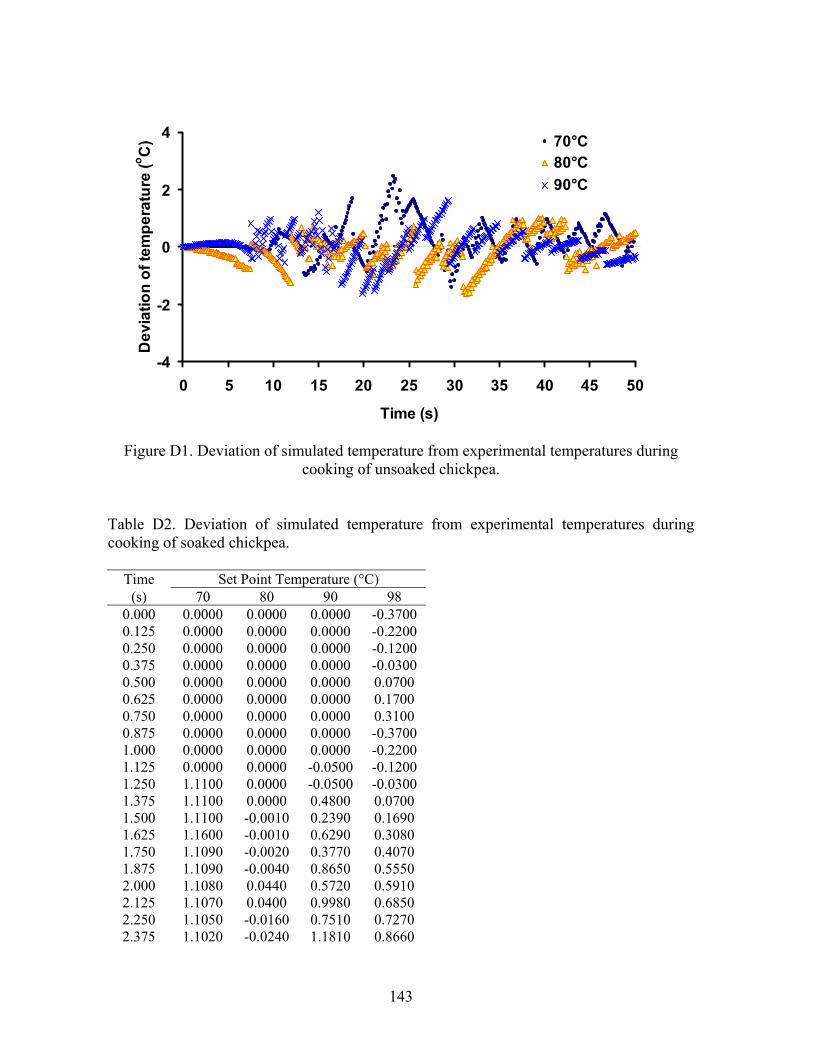
143

-4

-2

0

2

4

0 5 10 15 20 25 30 35 40 45 50

Time (s)

Dev

iatio

n of

tem

pera

ture

(o C) 70°C

80°C90°C

Figure D1. Deviation of simulated temperature from experimental temperatures during

cooking of unsoaked chickpea.

Table D2. Deviation of simulated temperature from experimental temperatures during cooking of soaked chickpea.

Time Set Point Temperature (°C) (s) 70 80 90 98

0.000 0.0000 0.0000 0.0000 -0.3700 0.125 0.0000 0.0000 0.0000 -0.2200 0.250 0.0000 0.0000 0.0000 -0.1200 0.375 0.0000 0.0000 0.0000 -0.0300 0.500 0.0000 0.0000 0.0000 0.0700 0.625 0.0000 0.0000 0.0000 0.1700 0.750 0.0000 0.0000 0.0000 0.3100 0.875 0.0000 0.0000 0.0000 -0.3700 1.000 0.0000 0.0000 0.0000 -0.2200 1.125 0.0000 0.0000 -0.0500 -0.1200 1.250 1.1100 0.0000 -0.0500 -0.0300 1.375 1.1100 0.0000 0.4800 0.0700 1.500 1.1100 -0.0010 0.2390 0.1690 1.625 1.1600 -0.0010 0.6290 0.3080 1.750 1.1090 -0.0020 0.3770 0.4070 1.875 1.1090 -0.0040 0.8650 0.5550 2.000 1.1080 0.0440 0.5720 0.5910 2.125 1.1070 0.0400 0.9980 0.6850 2.250 1.1050 -0.0160 0.7510 0.7270 2.375 1.1020 -0.0240 1.1810 0.8660

144

2.500 1.0990 -0.0350 0.9180 0.8000 2.625 1.0940 0.0000 1.3400 0.9690 2.750 1.0870 0.0310 1.0780 1.0930 2.875 1.0780 0.1070 1.4790 1.3490 3.000 1.0680 0.1270 1.2030 1.1680 3.125 1.0540 0.1910 1.6000 1.4470 3.250 1.0370 0.1870 1.0180 1.2960 3.375 1.0170 0.2350 -0.4040 1.4140 3.500 0.9930 0.2240 0.4930 1.2290 3.625 0.9650 0.2930 -0.4610 1.3320 3.750 0.9320 0.3120 0.5530 0.2000 3.875 0.8930 0.4100 0.6850 -0.6050 4.000 0.8500 0.4070 -0.2070 -0.3570 4.125 0.8010 0.4420 0.9570 -0.2240 4.250 0.7450 0.8950 -1.6630 -0.0570 4.375 0.6840 0.4650 0.6930 -0.0970 4.500 0.5650 0.3630 1.3330 -0.0140 4.625 0.5400 0.4380 -1.2710 0.6320 4.750 0.4080 0.3100 0.0200 0.6320 4.875 0.3690 0.4080 0.4150 0.4240 5.000 0.2220 0.2450 1.0960 0.3390 5.125 0.1180 0.3180 0.2120 0.4770 5.250 -0.0430 0.0880 0.8130 0.4590 5.375 -0.1120 0.1860 -1.8800 0.8540 5.500 -0.2880 -0.0680 0.4230 0.6140 5.625 -0.4210 0.0070 -0.4580 0.3480 5.750 -0.5620 0.3990 0.2680 0.6980 5.875 -0.7100 0.0600 0.8000 0.5130 6.000 -0.8650 0.1510 -0.1290 0.1540 6.125 -1.0270 -0.2090 0.3290 0.6010 6.250 -1.1960 -0.1890 0.7660 0.1760 6.375 -1.3710 -0.6180 -0.3380 -0.0710 6.500 -1.5540 -0.5270 0.3280 -0.4700 6.625 -1.7420 -0.0040 2.3140 -0.2100 6.750 -1.9360 -0.5100 1.2800 -0.6800 6.875 -2.0370 -0.2930 1.6680 -0.9210 7.000 -1.7130 -0.3340 0.6170 -1.3600 7.125 -1.2140 -0.9510 1.1280 -1.0980 7.250 -0.8510 -0.8050 2.1520 -1.4140 7.375 -0.3630 -1.3850 2.5990 -0.5480 7.500 0.1310 -1.2500 -0.0400 -0.8780 7.625 0.5700 -0.9910 2.5750 -1.3040 7.750 0.9450 -0.8660 0.8250 -0.8470 7.875 1.1850 -1.5160 1.3000 -1.1440 8.000 1.4120 -1.4000 0.1610 -0.9770 8.125 1.4050 -2.0070 0.6680 -1.2430 8.250 1.4840 -1.9070 0.9410 -0.9840 8.375 1.4710 -2.6200 1.0610 -1.2070 8.500 1.4940 -1.5160 -0.0410 -0.9640 8.625 1.4250 -1.6140 0.9240 -1.1930

145

8.750 -1.4530 -0.1530 1.4070 -1.7130 8.875 -1.3790 -1.4340 0.3480 -1.5160 9.000 -1.3930 -0.6370 0.4090 -2.0400 9.125 -1.2650 -1.3000 -0.0920 -1.1440 9.250 -1.6550 -0.0440 -1.1530 -1.3390 9.375 -1.1930 0.2320 -1.0950 -1.8540 9.500 -1.2500 0.5470 -0.7070 -1.6290 9.625 -1.1160 -0.3970 -0.4580 -1.8140 9.750 -1.1300 0.0190 -0.2090 -1.5380 9.875 -0.9940 -0.3750 -1.0790 -2.0610

10.000 -0.9970 0.2730 -0.3190 -1.3630

-4

-2

0

2

4

0 5 10 15 20 25 30 35 40 45 50

Time (s)

Dev

iatio

n of

tem

pera

ture

(o C) 70°C 80°C

90°C 98°C

Figure D2. Deviation of simulated temperature from experimental temperatures during

cooking of soaked chickpea.

146

Table D3. Deviation of simulated and experimental moisture ratio during cooking of unsoaked chickpea.

Time Set Point Moisture Ratio

h 70°C 80°C 90°C 98°C 0 0.00 0.00 0.00 0.00 1 -0.01 -0.07 -0.02 -0.14 2 -0.05 -0.04 0.01 0.04 3 0.01 -0.01 0.09 -0.01 4 -0.02 0.04 0.04 -0.06 5 0.00 0.05 0.01 0.00 6 0.03 0.02 -0.05 7 -0.03 -0.04 -0.02 8 -0.02 -0.12 -0.01 9 -0.01 -0.08 -0.01

10 0.00 -0.06 0.00 11 -0.10 -0.04 12 0.00 0.00

-0.15

-0.05

0.05

0.15

0 2 4 6 8 10 12

Time (h)

Dev

iatio

n of

moi

stur

e ra

tio

70°C 80°C

90°C 98.7°C

Figure D3. Deviation of simulated moisture ratio from experimental moisture ratio changes

during cooking of unsoaked chickpea.

147

Table D4: Deviation of simulated and experimental moisture ratio during cooking of soaked chickpea.

Time Set Point Moisture Ratio

h 70°C 80°C 90°C 98°C 0 0.00 0.00 0.00 0.00 1 -0.01 -0.08 0.09 0.04 2 0.01 -0.10 0.08 0.00 3 0.06 0.03 0.02 -0.01 4 -0.01 0.01 -0.01 0.00 5 0.00 -0.01 6 0.03 -0.04 7 -0.01 -0.04 8 -0.03 -0.02 9 -0.09 -0.01

10 -0.06 0.00 11 -0.04 12 0.00

-0.15

-0.05

0.05

0.15

0 2 4 6 8 10 12

Time (h)

Dev

iatio

n of

moi

stur

e ra

tio

70°C 80°C90°C 98.7°C

Figure D4. Deviation of simulated moisture ratio from experimental moisture ratio changes during cooking of soaked chickpea.

148

APPENDIX E

Experimental and Simulated Results. Table E1. Experimental and simulated temperatures during cooking of unsoaked kabuli chickpea. 70°C 80°C 90°C 98°C

Time Exp Sim Exp Sim Exp Sim Exp Sim (s) (°C) (°C) (°C) (°C) (°C) (°C) (°C) (°C)

0.000 24.84 24.84 23.87 23.87 26.51 26.51 25.76 25.80 0.125 24.89 24.84 23.87 23.87 26.51 26.51 25.76 25.80 0.250 24.84 24.84 23.87 23.87 26.51 26.51 25.76 25.80 0.375 24.89 24.84 23.87 23.87 26.56 26.51 25.71 25.80 0.500 24.84 24.84 23.82 23.87 26.51 26.51 25.76 25.80 0.625 24.84 24.84 23.87 23.87 26.56 26.51 25.76 25.80 1.000 24.84 24.84 23.82 23.87 26.51 26.51 25.71 25.80 3.500 24.84 24.84 23.62 23.87 26.65 26.52 25.70 25.86 6.000 24.84 24.85 23.34 23.91 26.75 26.66 30.15 26.85 8.500 24.84 24.94 24.14 24.18 27.89 27.34 34.93 29.94

11.000 25.66 25.22 24.14 24.96 28.71 28.86 39.94 34.99 13.500 24.80 25.78 26.36 26.40 31.42 31.24 45.69 41.10 16.000 26.91 26.66 27.85 28.45 34.21 34.31 51.64 47.48 18.000 29.27 27.85 31.04 30.96 37.12 37.79 57.07 53.64 24.250 32.24 31.43 37.69 37.60 46.45 46.33 67.47 65.90 30.500 35.31 35.95 44.94 44.85 54.94 55.01 75.70 75.84 36.625 41.06 40.37 51.45 51.18 62.48 62.24 81.40 82.76 43.000 44.81 44.59 56.07 56.73 68.51 68.33 86.30 87.80 49.250 48.21 48.23 61.50 61.17 72.60 73.07 89.90 91.22 55.500 51.41 51.36 64.13 64.76 76.70 76.81 92.60 93.60 61.750 53.18 54.02 67.85 67.64 80.00 79.74 94.50 95.25 68.000 56.39 56.26 70.40 69.95 82.50 82.03 95.90 96.40 74.250 59.23 58.14 72.60 71.79 84.30 83.82 97.00 97.19 80.500 59.90 59.72 74.20 73.27 85.70 85.22 97.80 97.75 86.750 61.37 61.04 75.20 74.45 86.70 86.31 98.40 98.13 93.000 63.02 62.14 75.80 75.39 87.40 87.16 98.80 98.40 99.250 63.25 63.06 76.80 76.14 88.00 87.83 98.90 98.58

105.500 64.09 63.83 77.30 76.73 88.40 88.35 98.90 98.71 111.750 64.67 64.47 77.50 77.21 88.70 88.75 98.90 98.80 117.750 65.47 64.99 77.80 77.58 89.00 89.06 98.90 98.86 124.250 66.04 65.45 78.00 77.90 89.30 89.32 98.90 98.90 130.500 66.44 65.83 78.20 78.14 89.50 89.51 98.90 98.93 136.750 66.71 66.14 77.90 78.33 89.60 89.66 98.90 98.95 143.000 66.88 66.40 77.90 78.49 89.70 89.78 98.90 98.97 149.250 67.10 66.62 78.50 78.61 89.80 89.87 98.90 98.98 155.500 67.54 66.80 78.50 78.71 89.90 89.94 98.90 98.98 161.750 67.37 66.95 78.50 78.79 90.00 90.00 98.90 98.99 168.000 67.19 67.07 78.60 78.85 90.00 90.04 98.90 98.99 174.250 66.97 67.18 78.50 78.90 90.00 90.08 98.93 99.00 180.500 66.88 67.27 78.60 78.94 90.00 90.11 98.93 99.00 186.750 66.92 67.34 78.60 78.97 90.00 90.13 98.93 99.00

149

Table E2: Experimental and simulated temperatures during cooking of soaked kabuli chickpea. 70°C 80°C 90°C 98°C

Time Exp Sim Exp Sim Exp Sim Exp Sim (s) (°C) (°C) (°C) (°C) (°C) (°C) (°C) (°C)

0.000 20.84 20.84 20.61 20.61 20.54 20.54 20.12 20.49 0.125 20.84 20.84 20.61 20.61 20.54 20.54 20.27 20.49 0.250 20.84 20.84 20.61 20.61 20.54 20.54 20.37 20.49 0.375 20.84 20.84 20.61 20.61 20.54 20.54 20.46 20.49 0.500 20.84 20.84 20.61 20.61 20.54 20.54 20.56 20.49 0.625 20.84 20.84 20.61 20.61 20.54 20.54 20.66 20.49 0.750 20.84 20.84 20.61 20.61 20.54 20.54 20.80 20.49 0.875 20.84 20.84 20.61 20.61 20.54 20.54 20.12 20.49 1.000 20.84 20.84 20.61 20.61 20.54 20.54 20.27 20.49 3.500 21.95 20.96 21.15 20.93 21.41 20.92 22.16 20.93 6.000 21.85 22.72 24.77 24.62 25.12 25.25 26.06 25.91 8.500 28.52 27.03 30.70 32.22 34.03 34.07 34.95 35.91

11.000 33.70 32.89 38.10 40.82 42.31 44.01 47.08 47.10 13.500 39.24 38.42 48.79 48.69 53.22 53.05 55.69 57.23 16.000 44.35 43.62 55.57 55.29 59.67 60.62 66.81 65.67 18.000 47.93 47.29 59.17 59.65 65.07 65.61 71.10 71.23 24.250 56.16 55.77 68.62 69.04 76.20 76.34 84.40 83.15 30.500 61.03 60.80 74.70 74.16 81.50 82.19 89.70 89.61 36.500 63.77 63.63 77.00 76.85 84.00 85.27 93.20 93.00 43.000 65.49 65.41 77.90 78.44 84.80 87.08 94.80 94.98 49.250 66.43 66.38 77.90 79.25 87.10 88.01 96.00 95.99 55.500 67.15 66.95 78.50 79.68 87.30 88.51 96.10 96.53 61.750 66.97 67.27 78.80 79.92 87.50 88.78 96.10 96.82 68.000 67.15 67.46 79.00 80.05 87.60 88.93 96.40 96.98 74.250 67.06 67.57 79.10 80.12 87.90 89.01 96.70 97.07 80.500 67.32 67.63 79.20 80.16 87.90 89.05 96.50 97.11 86.750 67.45 67.67 78.90 80.18 88.00 89.07 96.50 97.14 93.000 67.50 67.69 79.00 80.19 88.10 89.09 96.10 97.15 99.250 67.63 67.70 78.90 80.19 87.90 89.09 96.70 97.16

105.500 67.67 67.71 79.10 80.20 88.20 89.10 96.40 97.16 111.750 67.89 67.71 80.00 80.20 88.20 89.10 96.30 97.16 117.625 67.45 67.71 79.00 80.20 88.60 89.10 97.20 97.17 124.250 67.72 67.71 80.00 80.20 88.10 89.10 96.30 97.17 130.500 67.41 67.71 80.00 80.20 88.00 89.10 96.70 97.17 136.750 67.14 67.71 79.90 80.20 87.50 89.10 96.40 97.17 143.000 66.97 67.71 80.00 80.20 88.90 89.10 95.90 97.17 149.250 66.92 67.71 79.00 80.20 88.60 89.10 96.50 97.17 155.500 67.06 67.71 79.00 80.20 89.10 89.10 96.10 97.17 161.750 66.92 67.71 79.90 80.20 88.80 89.10 96.70 97.17 168.000 66.92 67.71 79.30 80.20 88.50 89.10 95.60 97.17 174.250 67.15 67.71 80.10 80.20 88.40 89.10 96.20 97.17 180.500 67.37 67.71 80.00 80.20 87.80 89.10 95.90 97.17 186.750 67.50 67.71 79.70 80.20 87.80 89.10 96.10 97.17 193.000 67.58 67.71 79.20 80.20 87.50 89.10 96.10 97.17

150

Table E3: Experimental and simulated moisture ratio during cooking of unsoaked kabuli chickpea. 70°C 80°C 90°C 98.7°C

Time Exp Sim Exp Sim Exp Sim Exp Sim (h) MR MR MR MR MR MR MR MR 0 1.00 1.00 1.00 1.00 1.00 1.00 1.00 1.00 1 0.99 1.00 0.92 0.99 0.89 0.91 0.63 0.77 2 0.89 0.94 0.83 0.87 0.57 0.56 0.38 0.34 3 0.81 0.80 0.65 0.66 0.39 0.30 0.13 0.14 4 0.62 0.64 0.52 0.48 0.20 0.16 0.00 0.06 5 0.50 0.50 0.39 0.34 0.10 0.09 0.00 0.00 6 0.41 0.38 0.26 0.24 0.00 0.05 7 0.26 0.29 0.13 0.17 0.00 0.02 8 0.20 0.22 0.00 0.12 0.00 0.01 9 0.15 0.17 0.00 0.08 0.00 0.01

10 0.13 0.13 0.00 0.06 0.00 0.00 11 0.00 0.10 0.00 0.04

Table E4: Experimental vs simulated moisture ratio during cooking of soaked kabuli chickpea. 70°C 80°C 90°C 98°C

Time Exp Sim Exp Sim Exp Sim Exp Sim (h) MR MR MR MR MR MR MR MR 0 1.00 1.00 1.00 1.00 1.00 1.00 1.00 1.00 1 0.98 0.99 0.87 0.94 0.58 0.49 0.37 0.33 2 0.89 0.88 0.55 0.64 0.20 0.12 0.05 0.06 3 0.73 0.67 0.42 0.38 0.05 0.03 0.00 0.01 4 0.48 0.49 0.24 0.22 0.00 0.01 0.00 0.00 5 0.35 0.35 0.12 0.13 0.00 0.00 6 0.28 0.25 0.04 0.07 7 0.17 0.17 0.00 0.04 8 0.09 0.12 0.00 0.02 9 0.00 0.09 0.00 0.01

10 0.00 0.06 0.00 0.00 11 0.00 0.04

151

APPENDIX F

Experimental Values Shown in Replicates. Table F1. Moisture content of chickpea seed samples used in experiments.

Level Replicate MC Mean SD CV (% w.b.) (% w.b.) (% w.b.) (%)

1 1 9.69 2 9.97 3 9.93 9.86 0.15 1.55 2 1 13.49 2 13.13 3 12.99 13.20 0.26 1.98 3 1 18.15 2 18.16 3 18.20 18.17 0.02 0.13 4 1 26.60 2 26.52 3 26.49 26.54 0.05 0.22 5 1 37.74 2 37.94 3 37.99 37.89 0.13 0.35 6 1 56.17 2 56.15 3 55.58 55.97 0.33 0.60 7 1 65.48 2 64.88 3 65.35 65.24 0.31 0.48

152

Table F2. Particle density of chickpea as a function of moisture content.

Moisture content Trial Density Mean SD CV (% w.b.) (kg/m3) (kg/m3) (kg/m3) (%)

9.86 1 1445.41 9.86 2 1465.53 9.86 3 1437.34 9.86 4 1462.60 9.86 5 1486.32 1459.44 19.07 1.31 13.20 1 1392.80 13.20 2 1360.50 13.20 3 1395.38 13.20 4 1415.28 13.20 5 1411.33 1395.06 21.63 1.55 18.17 1 1369.91 18.17 2 1408.75 18.17 3 1388.63 18.17 4 1397.26 18.17 5 1356.34 1384.18 21.05 1.52 25.10 1 1363.80 25.10 2 1334.30 25.10 3 1341.57 25.10 4 1344.06 25.10 5 1342.26 1345.20 11.04 0.82 35.89 1 1298.98 35.89 2 1321.12 35.89 3 1299.97 35.89 4 1306.50 35.89 5 1301.00 1305.51 9.19 0.70 55.97 1 1207.76 55.97 2 1190.83 55.97 3 1211.27 55.97 4 1191.18 55.97 5 1209.52 1202.11 10.21 0.85 65.24 1 1108.37 65.24 2 1107.64 65.24 3 1109.51 65.24 4 1115.70 65.24 5 1107.87 1109.82 3.36 0.30

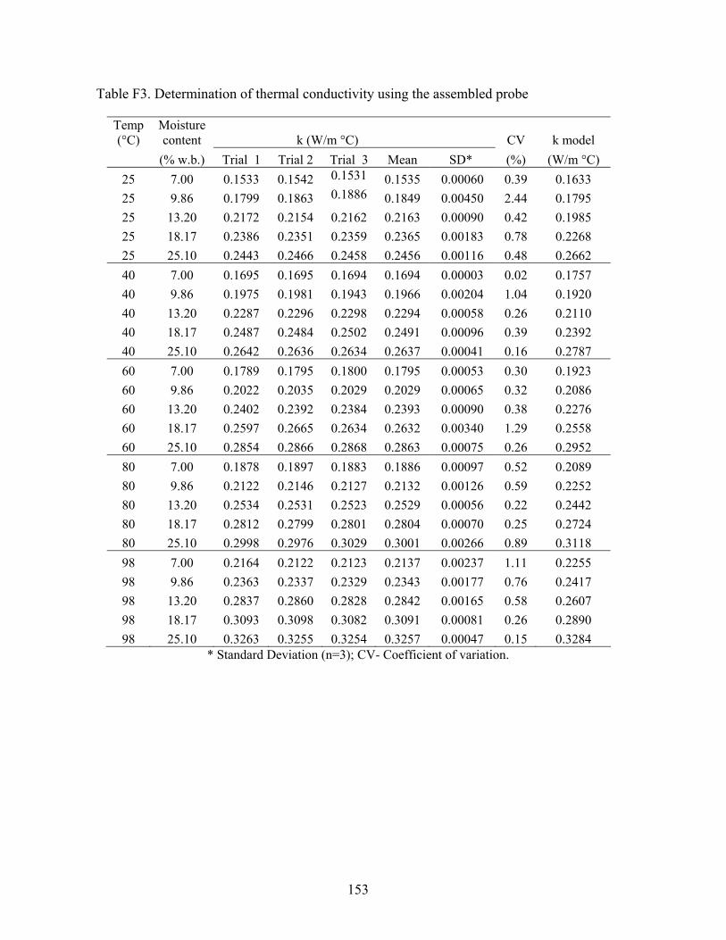
153

Table F3. Determination of thermal conductivity using the assembled probe

Temp (°C)

Moisture content k (W/m °C) CV k model

(% w.b.) Trial 1 Trial 2 Trial 3 Mean SD* (%) (W/m °C) 25 7.00 0.1533 0.1542 0.1531 0.1535 0.00060 0.39 0.1633 25 9.86 0.1799 0.1863 0.1886 0.1849 0.00450 2.44 0.1795 25 13.20 0.2172 0.2154 0.2162 0.2163 0.00090 0.42 0.1985 25 18.17 0.2386 0.2351 0.2359 0.2365 0.00183 0.78 0.2268 25 25.10 0.2443 0.2466 0.2458 0.2456 0.00116 0.48 0.2662 40 7.00 0.1695 0.1695 0.1694 0.1694 0.00003 0.02 0.1757 40 9.86 0.1975 0.1981 0.1943 0.1966 0.00204 1.04 0.1920 40 13.20 0.2287 0.2296 0.2298 0.2294 0.00058 0.26 0.2110 40 18.17 0.2487 0.2484 0.2502 0.2491 0.00096 0.39 0.2392 40 25.10 0.2642 0.2636 0.2634 0.2637 0.00041 0.16 0.2787 60 7.00 0.1789 0.1795 0.1800 0.1795 0.00053 0.30 0.1923 60 9.86 0.2022 0.2035 0.2029 0.2029 0.00065 0.32 0.2086 60 13.20 0.2402 0.2392 0.2384 0.2393 0.00090 0.38 0.2276 60 18.17 0.2597 0.2665 0.2634 0.2632 0.00340 1.29 0.2558 60 25.10 0.2854 0.2866 0.2868 0.2863 0.00075 0.26 0.2952 80 7.00 0.1878 0.1897 0.1883 0.1886 0.00097 0.52 0.2089 80 9.86 0.2122 0.2146 0.2127 0.2132 0.00126 0.59 0.2252 80 13.20 0.2534 0.2531 0.2523 0.2529 0.00056 0.22 0.2442 80 18.17 0.2812 0.2799 0.2801 0.2804 0.00070 0.25 0.2724 80 25.10 0.2998 0.2976 0.3029 0.3001 0.00266 0.89 0.3118 98 7.00 0.2164 0.2122 0.2123 0.2137 0.00237 1.11 0.2255 98 9.86 0.2363 0.2337 0.2329 0.2343 0.00177 0.76 0.2417 98 13.20 0.2837 0.2860 0.2828 0.2842 0.00165 0.58 0.2607 98 18.17 0.3093 0.3098 0.3082 0.3091 0.00081 0.26 0.2890 98 25.10 0.3263 0.3255 0.3254 0.3257 0.00047 0.15 0.3284

* Standard Deviation (n=3); CV- Coefficient of variation.

154

Table F4. Heat capacity of assembled calorimeter. Trial Mean SD CV 1 2 3 (%)

mw (kg) 2.034 2.048 2.025

Te (°C) 46.41 46.44 47.43 Toc (°C) 26.00 25.99 26.27

Tow (°C) 48.37 48.25 49.37

dT/dt (°C/min) -0.0300 -0.0254 -0.0272

te (min) 27.5 27 27.5

Hc (kJ/°C) 0.4546 0.4550 0.4608 0.4568 0.0034 0.75

where:

mw = mass of water (kg),

Te = temperature of water when it reaches equilibrium with the calorimeter (°C),

Toc = initial temperature of the calorimeter (°C),

Tow = initial temperature of the water (°C),

dT/dt = rate of temperature change (from graph of time and temperature) (°C/min),

te = time when water reaches equilibrium with the calorimeter (min),

Hc = heat capacity of calorimeter (kJ/°C), and

cpw = specific heat of water (4.182kJ/°C).

155

Table F5. Specific heat values for chickpea by assembled calorimeter method.

Moisture content Specific heat (kJ/kg°C) CV cp model (%) Trial # 1 Trial # 2 Trial # 3 Mean SD (%) (kJ/ kg°C) 9.86 1.3772 1.3897 1.3578 1.3749 0.01 1.17 1.5785 13.2 1.5684 1.5812 1.5954 1.5817 0.01 0.85 1.6348

18.17 1.8434 1.8601 1.8452 1.8496 0.00 0.49 1.7185 25.1 1.9823 1.9408 1.9758 1.9663 0.02 1.14 1.8353

35.89 2.1690 2.0774 2.1587 2.1350 0.05 2.35 2.0171 55.97 2.2333 2.2492 2.3089 2.2638 0.03 1.76 2.3555 65.24 2.4645 2.4936 2.4824 2.4802 0.01 0.59 2.5117

156

Table F6. Specific heat values of chickpea by DSC.

Moisture content Temperature Specific heat cp model (% w.b.) (°C) (kJ/kg°C) (kJ/ kg°C)

9.86 30 1.154 1.377 9.86 40 1.207 1.426 9.86 50 1.264 1.475 9.86 60 1.312 1.524 9.86 70 1.350 1.573 9.86 80 1.384 1.622 18.17 30 1.713 1.521 18.17 40 1.760 1.570 18.17 50 1.807 1.619 18.17 60 1.849 1.668 18.17 70 1.895 1.717 18.17 80 1.938 1.766 26.54 30 1.748 1.665 26.54 40 1.807 1.714 26.54 50 1.869 1.763 26.54 60 1.927 1.812 26.54 70 1.988 1.861 26.54 80 2.036 1.910 37.89 30 1.866 1.860 37.89 40 1.913 1.909 37.89 50 1.962 1.959 37.89 60 2.016 2.008 37.89 70 2.070 2.057 37.89 80 2.123 2.106 55.97 30 2.078 2.172 55.97 40 2.131 2.221 55.97 50 2.185 2.270 55.97 60 2.236 2.319 55.97 70 2.284 2.368 55.97 80 2.333 2.417 65.24 30 2.358 2.332 65.24 40 2.398 2.381 65.24 50 2.439 2.430 65.24 60 2.485 2.479 65.24 70 2.525 2.528 65.24 80 2.568 2.577

157

Table F7. Thermal diffusivity values of kabuli chickpea.

Moisture content Thermal diffusivity Mean SD CV (% w.b.) (× 10-7m2/s) (× 10-7m2/s) (×10-7m2/s) (%)

9.86 0.9201 9.86 0.9118 9.86 0.9332 0.9217 0.0108 1.17

18.17 1.0149 18.17 1.0366 18.17 1.0182 1.0233 0.0117 1.14 26.54 1.4936 26.54 1.5595 26.54 1.5008 1.5180 0.0362 2.38 37.89 2.2412 37.89 2.2254 37.89 2.1679 2.2115 0.0386 1.75 55.97 2.3350 55.97 2.3054 55.97 2.3167 2.3191 0.0149 0.64 65.24 2.5350 65.24 2.5054 65.24 2.5167 2.5191 0.1490 0.59

158

Table F8. Determination of solids loss during soaking of chickpea.

Temperature Trial # Solids loss Mean SD CV (°C) (%) (%) (%) (%) 100 1 6.31 100 2 6.20 100 3 6.22 6.24 0.05 0.94 80 1 5.29 80 2 5.46 80 3 5.09 5.28 0.18 3.51 60 1 4.05 60 2 3.80 60 3 4.03 3.96 0.13 3.51 40 1 2.63 40 2 2.71 40 3 2.50 2.61 0.10 4.06 25 1 1.99 25 2 1.98 25 3 1.87 1.95 0.06 3.42