Health Monitoring for Airframe Structural Characterization · PDF fileNASA/CR-2002-211428...
163
NASA/CR-2002-211428 Health Monitoring for Airframe Characterization Structural Thomas E. Munns, Renee M. Kent, and Antony Bartolini ARINC, Inc., Annapolis, Maryland Charles B. Gause, Jason W. Borinski, Jason Dietz, Jennifer L. Elster, Clark Boyd, Larry Vicari, and Kevin Cooper Luna Innovations, Blacksburg, Virginia Asok Ray, Eric Keller, Vadlamani Venkata, and S. C. Sastry The Pennsylvania State University, University Park, Pennsylvania February 2002 https://ntrs.nasa.gov/search.jsp?R=20020030899 2018-05-17T13:20:11+00:00Z
Transcript of Health Monitoring for Airframe Structural Characterization · PDF fileNASA/CR-2002-211428...

NASA/CR-2002-211428
Health Monitoring for AirframeCharacterization
Structural
Thomas E. Munns, Renee M. Kent, and Antony Bartolini
ARINC, Inc., Annapolis, Maryland
Charles B. Gause, Jason W. Borinski, Jason Dietz, Jennifer L. Elster, Clark Boyd, Larry Vicari,
and Kevin Cooper
Luna Innovations, Blacksburg, Virginia
Asok Ray, Eric Keller, Vadlamani Venkata, and S. C. Sastry
The Pennsylvania State University, University Park, Pennsylvania
February 2002
https://ntrs.nasa.gov/search.jsp?R=20020030899 2018-05-17T13:20:11+00:00Z

The NASA STI Program Office... in Profile
Since its founding, NASA has been dedicatedto the advancement of aeronautics and spacescience. The NASA Scientific and Technical
InfmTnation (STI) Program Office plays a key
part in helping NASA maintain this
important role.
The NASA STI Program Office is operated by
Langley Research Center, the lead center forNASA's scientific and technical information.
The NASA STI Program Office provides
access to the NASA STI Database, the
largest collection of aeronautical and space
science STI in the world. The Program Officeis also NASA's institutional mechanism for
disseminating the results of its research and
development activities. These results are
published by NASA in the NASA STI Report
Series, which includes the following report
types:
TECHNICAL PUBLICATION. Reports of
completed research or a major significant
phase of research that present the results
of NASA programs and include extensive
data or theoretical analysis. Includes
compilations of significant scientific andtechnical data and infmfnation deemed
to be of continuing reference value. NASA
counterpart of peer reviewed fmTnal
professional papers, but having less
stringent limitations on manuscript
length and extent of graphic
presentations.
TECHNICAL MEMORANDUM.
Scientific and technical findings that are
preliminary or of specialized interest,
e.g., quick release reports, working
papers, and bibliographies that containminimal annotation. Does not contain
extensive analysis.
CONTRACTOR REPORT. Scientific and
technical findings by NASA sponsored
contractors and grantees.
CONFERENCE PUBLICATION.
Collected papers fi'om scientific and
technical conferences, symposia,
seminars, or other meetings sponsored or
co sponsored by NASA.
SPECIAL PUBLICATION. Scientific,
technical, or historical information from
NASA programs, projects, and missions,
often concerned with subjects having
substantial public interest.
TECHNICAL TRANSLATION. English
language translations of foreign scientific
and technical material pertinent toNASA's mission.
Specialized services that complement the
STI Program Office's diverse offerings include
creating custom thesauri, building customized
databases, organizing and publishing
research results.., even providing videos.
For more information about the NASA STI
Program Office, see the following:
• Access the NASA STI Program Home
Page at http://vevew.sti.nasa.gov
• Email your question via the Intemet to
• Fax your question to the NASA STI
Help Desk at (301) 621 0134
• Telephone the NASA STI Help Desk at(301) 621 0390
Write to:
NASA STI Help Desk
NASA Center for AeroSpace Information7121 Standard Drive
Hanover, MD 21076 1320

NASA/CR-2002-211428
Health Monitoring for AirframeCharacterization
Structural
Thomas E. Munns, Renee M. Kent, and Antony Bartolini
ARINC, Inc., Annapolis, Maryland
Charles B. Gause, Jason W. Borinski, Jason Dietz, Jennifer L. Elster, Clark Boyd, Larry Vicari,
and Kevin Cooper
Luna Innovations, Blacksburg, Virginia
Asok Ray, Eric Keller, Vadlamani Venkata, and S. C. Sastry
The Pennsylvania State University, University Park, Pennsylvania
National Aeronautics and
Space Administration
Langley Research Center
Hampton, Virginia 23681 2199
Prepared for Langley Research Center
under Cooperative Agreement NCC 1 332
February 2002

Available from:
NASA Center for AeroSpace Information (CASI)7121 Standard Drive
Hanover, MD 21076 1320(301) 621 0390
National Technical Information Service (NTIS)
5285 Port Royal Road
Springfield, VA 22161 2171(703) 605 6000

EXECUTIVE SUMMARY
Structural health monitoring (SHM) is a critical consideration for overall condition
monitoring of aircraft systems. SHM of airframes for the identification and
characterization of structural degradation presents unique challenges. Traditionally, off-
line diagnostic models based on a statistical analysis of material degradation, operating
history, and anticipated perturbations in the flight profile have been used to characterize
airframe structures. Based on these analyses, a rigorous schedule of inspection and
maintenance actions is established to maintain the aircraft in an airworthy condition.
However, these existing diagnostic modeling techniques cannot elucidate the condition of
individual aircraft. Sensing and characterization of structural condition for specific
components of individual aircraft is required to meet the goals of NASA's Single Aircraft
Accident Prevention (SAAP) program.
The purpose of this project was to develop a multiplexed airframe structural sensor
prototype for on-board characterization of multiple and synergistic failure modes in
current and future airframes and to demonstrate the technologies in a laboratory setting.
Specifically, the purpose of this study was to establish requirements for structural health
monitoring systems, identify and characterize a prototype structural sensor system,
develop sensor interpretation algorithms, and demonstrate the sensor systems on
operationally realistic test articles. The structural sensing system was designed to provide
data sources for ARINC's Aircraft Condition Analysis and Management System
(ACAMS), which was developed in a complementary program.
The purpose of introducing SHM into commercial transports is to enhance aviation safety
by improving the effectiveness of the operator's continued airworthiness programs. The
primary consideration for assessing the effect of SHM systems on continued
airworthiness is to determine their potential influence on scheduled maintenance
programs and the potential to reduce unscheduled maintenance actions. SHM systems
could be an important factor in improving the effectiveness of inspection and
maintenance programs and enabling on-condition maintenance. Ultimately, these
improvements would increase air carrier profitability by reducing maintenance program
costs and increasing aircraft availability.
An important area of emphasis of this project was on sensors to detect aging mechanisms
for metallic airframe structures. An understanding of potential damage mechanisms,
structural design criteria and fail-safe features, structural maintenance philosophy was
needed to assess the efficacy of sensor-based system to monitor structural condition. The
structural degradation modes for commercial transport aircraft include low-cycle fatigue
(including widespread fatigue damage), high-cycle fatigue, corrosion (and stress
corrosion cracking), and accidental damage. The sensor system evaluation and sensor
development tasks of this project focused on the principal long-term aging mechanisms
for metallic transport aircraft structures--low-cycle fatigue and corrosion.

An arrayof multiplesensortypeswill berequiredto monitordamageevents,corrosionandenvironmentaldeterioration,andfatigue.Thisprogramfocusedonfiberopticsensors.Theselectedsensorswereevaluatedtovalidatetheirsuitabilityformonitoringagingdegradation;characterizethesensorperformancein aircraftenvironments;anddemonstrateplacementprocessesandmultiplexingschemes.Corrosionsensors(i.e.,moistureandmetalion sensors)andfatiguesensors(i.e.,strainandacousticemissionsensors)weredevelopedandevaluatedunderthisprogram.In addition,auniquemicromachinedmultimeasurandsensorconceptwasdevelopedanddemonstrated.Theresultsshowthatstructuraldegradationof aircraftmaterialscouldbeeffectivelydetectedandcharacterizedusingavailableandemergingsensors.
A keycomponentof thestructuralhealthmonitoringcapabilityis theability to interprettheinformationprovidedby sensorsystemin orderto characterizethestructuralcondition.Noveldeterministicandstochasticfatiguedamagedevelopmentandgrowthmodelshavebeendevelopedfor thisprogram.Thesemodelsenablerealtimecharacterizationandassessmentof structuralfatiguedamage.
Thegoalsfor implementingSHMsystemsareto improveaircraftsafetyandreduceoperationalandmaintenancecosts.ARINCrecommendsthat,basedonthesepromisinginitial results,thedevelopmentof SHMtechnologyasakeyelementof anintegratedvehiclehealthmanagementcapabilityshouldbecontinued.
ii

ABBREVIATIONS AND ACRONYMS
ACAMS
AE
AFM
ARMA
CCD
CMC
CMR
CMV
CPC
DSB
EDM
EFPI
FAA
FAR
FFT
FOQA
GDM
HCF
K-L
LCF
LPG
MPD
MSG
NASA
PEO
SAAP
SCC
SHM
Aircraft Condition Analysis and Management Systemacoustic emission
atomic force microscopy (AFM)
autoregressive moving average
charged-coupled device
Carboxymethylcellulose
certification maintenance requirementContinuous maintenance visits
corrosion preventive compounds
distributed feedback
electrostatic discharge machined
extrinsic Fabry-Perot interferometry
Federal Aviation Administration
federal aviation regulationfast Fourier transform
flight operations quality assurance
Gap division multiplexing
high-cycle fatigue
Karhunen-Lo6ve
low-cycle fatigue
long period grating
maintenance process data
maintenance steering group
National Aeronautics and Space Administration
poly (ethylene oxide)
probability density function
Single Aircraft Accident Prevention
stress corrosion cracking
structural health monitoring
iii

UVa
WDMWFD
Universityof Virginia
wavelengthdivisionmultiplexingwidespreadfatiguedamage
iv

CONTENTS
INTRODUCTION .................................................................................................. 1
1.0 BACKGROUND .................................................................................................. 1
1.1 PURPOSE ............................................................................................................. 2
1.2 SCOPE AND APPROACH ................................................................................. 2
IMPLEMENTATION REQUIREMENTS ANALYSIS ............................................. 4
INTRODUCTION ................................................................................................ 4
AIRLINE MAINTENANCE PROGRAMS ....................................................... 5
New Aircraft Models (MSG Process) ............................................................. 7
Maintenance Program Implementation ........................................................... 8
Program Review and Reliability Tracking ...................................................... 9
2.2 STRUCTURAL DEGRADATION MODES ................................................... 10
2.2.1 Fatigue ........................................................................................................... 11
2.2.2 Environmental Damage ................................................................................. 14
2.2.3 Accidental Damage ....................................................................................... 15
2.3 INTEGRATION AND UTILIZATION CONSIDERATIONS ..................... 16
2.4 DISCUSSION ..................................................................................................... 17
SENSOR SYSTEM DEVELOPMENT AND BASELINE CHARACTERIZATION 19
3.0 INTRODUCTION .............................................................................................. 19
3.1 FATIGUE SENSING ......................................................................................... 20
3.1.1 Bragg Grating Sensors ................................................................................... 203.1.2 EFPI Sensors ................................................................................................. 21
3.2 CORROSION SENSING .................................................................................. 28
3.2.1 LPG Moisture and Humidity Sensors ........................................................... 303.2.2 LPG Metal Ion Sensor ................................................................................... 33
3.3 COMBINED FAILURE MODES .................................................................... 35
3.4 ACCIDENTAL DAMAGE ............................................................................... 39
SENSOR DEMONSTRATION AND EVALUATION ................................................ 40
2.0
2.1
2.1.1
2.1.2
2.1.3
V

4.0
4.1
4.1.1
4.1.2
4.2
4.2.1
4.2.2
4.3
4.4
INTRODUCTION .............................................................................................. 40
CORROSION SENSOR TESTING ................................................................. 40
Simulated Lap Splice Testing ........................................................................ 40
Sensor Performance under Coatings ............................................................. 44
FATIGUE SENSOR TESTING ........................................................................ 51
Fiber Bragg Grating Sensors ......................................................................... 51EFPI Strain and Extensometer Sensor Tests ................................................. 57
TABLETOP SENSOR DEMONSTRATION ................................................. 62
SENSOR SYSTEM IMPLEMENTATION CONSIDERATIONS ............... 62
SENSOR DATA INTERPRETATION .................................................................. 65
5.0 INTRODUCTION .............................................................................................. 65
5.1
5.1.1
5.1.2
5.1.3
5.2
5.2.1
5.2.2
5.2.3
5.3
5.3.1
5.3.2
STATE-SPACE MODEL OF FATIGUE CRACK GROWTH ..................... 65
State-Space Model Formulation .................................................................... 67Model Validation with Test Data .................................................................. 72
Comparison of Computation Time ................................................................ 76
STOCHASTIC MODELING OF FATIGUE CRACK DAMAGE ............... 77
Model Formulation and Assessment ............................................................. 78
Analysis of Experimental Data ...................................................................... 82
Risk Analysis and Remaining Life Prediction .............................................. 91
DISCUSSION ..................................................................................................... 94
State-Space Model ......................................................................................... 94Stochastic Model ........................................................................................... 95
CONCLUSIONS AND RECOMMENDATIONS .................................................. 96
6.0 INTRODUCTION .............................................................................................. 96
6.1
6.1.1
6.1.2
HEALTH MONITORING SYSTEM REQUIREMENTS ............................ 96
Maintenance Program Requirements ............................................................ 96
Degradation Modes ....................................................................................... 97
6.2
6.2.1
6.2.2
6.2.3
6.2.4
SENSOR SYSTEM DEVELOPMENT ............................................................ 98
Corrosion ....................................................................................................... 98
Fatigue ........................................................................................................... 98
Combined Damage Modes ............................................................................ 99
Sensor System Implementation ..................................................................... 99
6.3 SENSOR DATA INTERPRETATION ............................................................ 99
vi

6.5 RECOMMENDATIONS................................................................................. 101
REFERENCES ................................................................................................. 102
APPENDIX: STATE-SPACE MODEL VALIDATION ........................................ 106
vii

Health Monitoring for Airframe Structural Characterization
SECTION 1INTRODUCTION
1.0 BACKGROUND
Structural health monitoring (HM) is a critical consideration for overall condition
monitoring of aircraft systems. In fact, significant inspection and maintenance of
structural components is required by the Federal Aviation Administration (FAA) in order
to maintain the continued airworthiness of commercial aircraft. For the air carriers, this
represents a considerable expense in aircraft maintenance; an expense that could be
significantly reduced with the implementation of an effective SHM capability. (Kent and
Murphy, 2000).
Traditionally, off-line diagnostic models based on a statistical analysis of material
degradation, operating history, and anticipated perturbations in the flight profile have
been used to characterize airframe structures. Based on these analyses, a rigorous
schedule of inspection and maintenance actions is established to maintain the aircraft in
an airworthy condition. However, these techniques cannot elucidate the condition of
individual aircraft. Sensing and characterization of structural condition for specific
components of individual aircraft is required to meet the goals of NASA's Single Aircraft
Accident Prevention (SAAP) program.
There are three key motivations to pursue sensor-based SHM capabilities. First, given the
inspection and maintenance techniques currently available, there is a potential that
indications of structural degradation could be missed. In general, structural safety
inspections can be difficult and tedious because: (1) the feature sizes for cracks and
corrosion are often small with respect to the resolution of the inspection methods, (2)
crucial structural details are often hidden or buried inside surrounding structure, making
access difficult, and (3) inspection of airframe components must include large areas with
many features to inspect. Even with the recent advances in automated ground-based
nondestructive evaluation methods, the vast majority of inspections are visual. Second,
SHM capability could enable on-condition maintenance of airframe structure. On-
condition maintenance of structures would simplify periodic checks, improve
productivity by minimizing aircraft downtime, and allow the maintenance program to be
tailored to the individual aircraft. Finally, SHM is an integral part of a comprehensive
condition analysis capability.
Advances in sensors are key enabling technologies to the realization of SHM capability.
Recent work has been focused on developing a suite of sensors that can be directly
embedded into the material system or attached to a structure with limited increase in cost,
weight, shape, or size. These sensors, when properly configured within the airframe
structure would create a distributed network capable of measuring strain, pressure,
temperature, and other key parameters. This sensor network would be capable of

detectingchangesin theoperationalenvironment(e.g.,thermomechanicalloading,flightprofileusage,materialstate,or internalcondition)andinitiatinganappropriateresponse(e.g.,transmittingthisinformationto acentralizedsignalprocessinganddatamanagementsystem).
Aspartof thelong-termeffortto implementSHMcapability,ARINC,in collaborationwithNASA, PennStateUniversity,andLunaInnovations,hasdevelopedanddemonstratedaprototypemultiplexedsensorsystemfor airframestructureandcompatiblereal-timedamagemodelsfor on-boardcharacterizationof multipleandsynergisticfailuremodesin currentandfutureairframes.Thegoalthatdrovethesedevelopmentswastomonitorstructuralconditionandanalyzestructuraldegradationasitoccurs,ratherthanto detectstructuralfailures.
1.1 PURPOSE
The purpose of this project was to develop a multiplexed airframe structural sensor
prototype for on-board characterization of multiple and synergistic failure modes in
current and future airframes and to demonstrate the technologies in a laboratory setting.
Specifically, the purpose of this study was to establish requirements for structural health
monitoring systems, identify and characterize a prototype structural sensor system,
develop sensor interpretation algorithms, and demonstrate the sensor systems on
operationally realistic test articles. The structural sensing system was designed to provide
data sources for ARINC's Aircraft Condition Analysis and Management System
(ACAMS), which was developed in a complementary program.
In previous work, we have shown that the implementation of advanced health monitoring
technologies will depend on (1) acceptance by operators, (2) the ability to gain approval
in the FAA certification process, and (3) compatibility with continued airworthiness
requirements (Munns, et al., 2000). With these factors in mind, a balance between a
technology development perspective and an end-use perspective was maintained
throughout the program so that the framework for acceptance, certification, and
implementation could be established.
1.2 SCOPE AND APPROACH
The scope of the study included: (1) determination of the operational constraints under
which the structural health monitoring system must perform; (2) development of a sensor
suite to provide a more comprehensive description of structural condition especially
related to known sources of structural degradation (specifically corrosion, fatigue
cracking, and stress behavior); (3) demonstration of the sensor technology in a laboratory
environment; and (4) development and validation of a dynamic model, formulated in the
state-space setting, of fatigue crack propagation in metallic materials.

In orderto achievethegoalsof theprogram,theARINCteamcompletedthefollowingtasks:
• Establishedrequirementsfor theimplementationof structuralhealthmonitoringsystems
• Identifiedandcharacterizedaprototypestructuralsensorsystemanddemonstratedthesensorsonrealistictestarticles
• Developedandvalidatedsensorinterpretationalgorithms
Theapproachtakenfor theimplementationrequirementsanalysisincluded:(1)assessingair carriermaintenance;and(2) identifyingandassessingimportantdegradationmodesfor agingairframestructuresthatwouldbetargetedby theSHMsystem.
Basedontheanalysisof theimplementationrequirements,astructuralsensingsystem,madeupof multiplesensortypes,wasdeveloped,characterized,anddemonstrated.Fiberopticsensorswerethepredominatesensorsusedfor thisstudy.Theselectedsensorswerecharacterizedto (1) determinetheirsuitabilityfor detectingtheimportantdegradationmechanisms;(2) identifymethodsto multiplexsensorsfor appropriatecoverage;and(3)assessrequirementsfor implementationin anintegratedhealthmanagementenvironment.Finally,theselectedsensorsweredemonstratedin structuraltestingenvironments.
A keycomponentof thestructuralhealthmonitoringcapabilityis theability to interprettheinformationprovidedby sensorsystemin orderto characterizethestructuralcondition.A noveldeterministicstate-spacefatiguegrowthmodelandstochasticmodelthataccountsfor thestatisticalnatureof damagedevelopmentprocessesweredevelopedto performreal-timecharacterizationandassessmentof structuralfatiguedamage.
Thestudyresultsareorganizedinto foursections:
• Section2 includesananalysisof requirementsfor theimplementationof SHMsystems
• Section3 includessensorsystemdevelopmentandbaselinecharacterization• Section4 includessensordemonstrationandevaluation• Section5 includessensordatainterpretation
Theconclusionsandrecommendationsarepresentedin Section6.

SECTION 2
IMPLEMENTATION REQUIREMENTS ANALYSIS
2.0 INTRODUCTION
Aging of aircraft structures, or the systematic degradation of structural components
resulting from exposure to the service environment was brought to attention of the
commercial transport industry as a result of 1988 Aloha Airlines 737 accident (NTSB
1988). This accident raised concerns that structures could lose their inherent fail-safety as
a result of fatigue damage or extensive corrosion. In response to this problem, the FAA
and the aircraft industry increased the frequency and requirements for periodic
inspections for older aircraft models (> 14 years of service). In addition, the damage
tolerance and durability requirements of FAR 25 (§25.571) were revised to address aging
structure issues. With the combined effects of increased inspection, more stringent
maintenance requirements, and increased aircraft utilization--along with the fact that
high-time "current generation" aircraft (e.g., 757, 767, A-300, MD-80) are moving into
the aging category--SHM capability has become more attractive for application incommercial aviation.
In this context, this section is focused on an analysis of the requirements for integrating
an advanced SHM system into an existing air carrier maintenance program. One of the
keys to implementation of advanced SHM technologies includes the compatibility of the
SHM capability with current and emerging FAA guidelines as well as acceptance by the
air carriers and viability of utilizing the SHM system in the airline operational
environment. Therefore, we report on SHM system requirements predicated on balancing
the characteristics, attributes, capabilities, and limitations of the state of the art in sensor
technology, data analysis, and decision support technologies, with existing and projected
aircraft maintenance and safety concepts.
There are three main objectives for integrating a sensing and analysis system into aircraftstructures:
• Ensure that the component is optimally manufactured to meet all relevant
operational specifications and criteria (baseline condition assessment)
• Monitor the condition and performance of the component throughout its servicelife
• Monitor the structural integrity of the component during its operationalutilization
The purpose of this section is to identify requirements for sensing, diagnostics, and
prognostics to develop and implement a health monitoring system for commercial
airframe structures. These requirements were developed based on an assessment of
operators maintenance programs and an analysis of aircraft structural degradation modes.

2.1 AIRLINE MAINTENANCE PROGRAMS
In order to realize the benefits that would be afforded by implementation and utilization
of SHM technologies, it was important to understand how these capabilities would be
integrated with the current maintenance infrastructure used by the airlines. The first step
in this process was to develop an understanding of the maintenance concepts that the
airlines currently use before trying to address integration of SHM technology. Once the
applicability and reliability of SHM systems has been proven, the overall acceptance by
the end user will require integration of SHM systems with existing systems and
capabilities.
In order for SHM systems to be an integral part of the operator's structural maintenance
programs, they would be required to (1) automate or improve inspections and tests; (2)
detect fault precursors so that maintenance or replacement activities can be anticipated
and scheduled; and (3) include the data collection and analysis functions associated with
maintenance program review.
Operators of commercial aircraft develop and implement maintenance and preventive
maintenance programs, not only to comply with regulations and guard against effects of
potential life-limiting defects, but also to maximize the availability of individual aircraft
(by minimizing aircraft down time) and to protect their considerable capital investment in
aircraft and equipment. The objectives of an effective maintenance program are to
accomplish the following in a cost-effective manner (ATA 1993):
• Ensure that the inherent component safety and reliability levels are realized
• Restore component safety and reliability to their inherent levels if deterioration
occurs
• Obtain information necessary for design improvement of components with
lower inherent reliability
The requirements for aircraft utilization have been steadily increasing in recent years.
Current schedules and route structures are such that aircraft could see as many as 16
hours per day of service. High utilization aircraft could approach 6000 hours in a year, a
number that has been steadily increasing over the past 10-15 years, resulting in fewer
opportunities to bring an aircraft in for maintenance (Edwards, 2000).
Although there are distinct differences in detail from airline to airline, most air carriers
adhere to similar concepts and protocols when performing maintenance on aircraft
structures. Continuous airworthiness maintenance programs are developed by the aircraft
operators and approved by the FAA. The basic elements of a continuous airworthiness
maintenance program includes the following (FAA 1980):
• Aircraft inspection, including routine inspections, servicing, and tests
performed on the aircraft at prescribed intervals
• Scheduled maintenance (i.e., maintenance tasks performed at prescribed
intervals), including replacement of life-limited items, components requiring

replacementforperiodicoverhaul,specialinspections,checksor testsfor on-conditionitems,andlubrication
• Unscheduled maintenance (i.e., maintenance tasks generated by the inspection
and scheduled maintenance elements, pilot reports, failure analyses, or other
indications of a need for maintenance)
• Engine, propeller, and appliance repair and overhaul
• Structural inspection program and airframe overhaul
• Required inspection items (i.e., safety-critical items)
• Maintenance manuals
There has been a gradual evolution of aircraft maintenance philosophy to embrace
reliability control methods as an integral part of an approved aircraft maintenance
program (FAA 1988). This transition is evident in the three approaches to preventive
maintenance currently applied to commercial transport components--hard time, on-
condition, and condition monitored--as described in the following paragraphs.
Early (first-generation) air carrier maintenance programs were developed under the
assumption that each functional component needed periodic disassembly for inspection.
This led to the implementation of hard time maintenance processes, where components
are removed from service when they reach a predetermined service parameter (e.g., flight
hours, flight cycles, or calendar time).
However, the majority of aircraft components do not exhibit old-age wear-out that would
be conducive to hard time maintenance. The principal reliability pattern for complex
aircraft systems is high initial failure rates, followed by random incidence of failure
throughout the remaining life (Edwards 2000). Replacing such components at a
prescribed age actually reduces overall reliability because the poor initial reliability is
introduced more often. This led to the implementation of on-condition maintenance
processes, where periodic visual inspection, measurements, tests or other means of
verification are used to establish component condition without disassembly, inspection, oroverhaul.
Finally, the industry and regulatory authorities developed methods to establish
maintenance program requirements by tracking component failure rates and maintaining
an acceptable level of reliability. Reliability methods identified components that respond
to neither hard time nor on-condition approaches. This led to the implementation of
condition monitoring maintenance processes, where component performance is
monitored and analyzed, but no formal services or inspections are scheduled, a
Airline maintenance programs include all three maintenance approaches as appropriate.
SHM systems could provide benefit to the operators in each of the maintenance scenarios
a This definition of condition monitoring differs from the definition traditionally used in nondestructiveevaluation or process controls. The traditional definition implies that parameters that would provideevidence of impending failure events are monitored. For the current definition performance relative to analert value indicating failure is monitored.

describedabove.First,hardtimecomponentscouldbeconvertedto oneof thereliability-basedapproachesby identifyingfaultsthatareprecursorsto failureandmonitoringthecomponentsusingaSHMsystem.Second,SHMsystemscouldbeusedto automatetheinspection,measurements,andtestsfor on-conditioncomponents.Finally,SHMsystemscouldbeusedto detecttheprecursorsto failurefor condition-monitoredcomponentssothatmaintenanceorreplacementactivitiescouldbeanticipatedandscheduled.
Maintenancetasksaredevelopedandimplementedfor individualcomponentsbycomponentmanufacturersandoperatorsbasedondetailedanalysesof componentperformance,potentialfailuremodesandconsequences,andreliabilityof similarcomponentsin service.Theapproachesusedby air carriersto identifymaintenancetasksareoutlinedin thefollowingsections.
2.1.1 New Aircraft Models (MSG Process)
Operators recommend initial maintenance tasks for new aircraft based on a detailed
analysis approach (ATA 1993). Each major subsystem is considered by a maintenance
steering group (MSG), which consists of senior maintenance engineers from each carrier
that will operate the aircraft type, as well as representatives of the manufacturer and the
FAA. The MSG identifies significant maintenance tasks in critical systems using a
rigorous evaluation process that includes the following general steps:
• Identify subsystem function
• Predict potential failure modes based on analysis or experience with similar
designs
• Analyze the failure modes using an established logic that considers
consequences of failure (e.g., affects safety, undetectable, operational impact,
economic impact)
• Write maintenance tasks and intervals based on the above assessment (e.g.,
lube/service, crew monitoring, operational check, inspection/functional check,
remove and restore, or remove and discard)
Structural designs are evaluated to identify potential structural failure processes, assess
the ability to detect indications of each failure mechanism, and determine the potential
consequences of each failure event (or multiple events acting simultaneously). Inspection,
maintenance, and modification tasks for structures are developed based on the results of
these analyses.
Once the MSG has identified the maintenance tasks, individual carriers add to or modify
the tasks for their operations to develop a maintenance list. At the same time, the
manufacturer develops a maintenance manual, which includes structural airworthiness
limitations, certification maintenance requirements (CMR) b, and servicing and lubrication
b CMRs are required periodic tasks that are established during airworthiness certification as operatinglimitations of the type certificate.

requirements.Basedontheirmaintenancemanual,themanufacturersdevelopmaintenanceprocessdata(MPD)andmaintenancetaskcards.Theair carriersusetheseresourcesto developtheirmaintenanceprogram.
2.1.2 Maintenance Program Implementation
Once maintenance tasks and intervals have been established, the air carrier must develop
an implementation plan, consistent with their operations and capabilities, to accomplish
scheduled maintenance tasks for each aircraft. In addition, the maintenance program must
have mechanisms to accomplish unscheduled maintenance so problems that arise out of
sequence with scheduled maintenance can be dealt with. The goals of an effective SHM
system are to anticipate required actions for scheduled maintenance visits and to save the
operators maintenance costs by reducing unscheduled maintenance actions.
2.1.2.1 Scheduled Maintenance
A typical maintenance program has a series of scheduled maintenance "checks," where
maintenance tasks are grouped so that they can be accomplished with minimal downtime.
The checks for a typical maintenance program are shown in Table 2-1. There are a
number of approaches to implementing inspection and maintenance intervals that comply
with manufacturers' suggestions and are complementary with the carriers' operations.
The following are examples of approaches to organizing maintenance tasks into checks
(Ake 2000):
• Block program - the aircraft is divided into inspection areas (zones) or systems
and all of the A-level or C-level checks are accomplished at an appropriate visit.
• Segmented program - each check interval is broken up into subintervals. For
example, instead of performing one large A-check at 4000 hours, the carrier can
perform 4 smaller checks at 1000, 2000, 3000, and 4000 hours. Either way, the
required work is done within the specified time.
• Phased program - similar to a segmented program except that all A-level
segments are completed within each B-level increment, and similarly for
higher-level checks.
• Continuous maintenance visits (CMV) program - individual tasks are assigned
an initial check and a prescribed interval. For example a task might start at the
second C-check (C2) and be repeated at every third C-check from then on (3C
interval).
The FAA does not prescribe how the operators must organize their tasks, so an acceptable
maintenance program could be organized using any of these methods or by combining themethods.
Table 2 -1. Typical Airline Scheduled Maintenance and Service PlanWhen Service is Performed Type of Service Performed Impact on Airline ServicePrior to each flight "Walk-around" - visual check of aircraft None
exterior and engines for damage, andleakage

Every2-7days
Every25-40days
Every45-75days
Every12-15months
Every2-5years(dependingonusageormandatoryinspection/modificationrequirements)
Servicecheck(linemaintenanceopportunity)- serviceconsumables(engineoils,hydraulicfluids,oxygen)andtireandbrakewearA-checks(linemaintenancecheck)-detailedcheckofaircraftandengineinterior,serviceandlubricationofsystems(e.g.,ignition,generators,cabin,airconditioning,hydraulics,structures,andlandinggear)B-checks(packagedA-checks)- torquetests,internalchecks,andflightcontrolsC-checks(basemaintenancevisit)-detailedinspectionandrepairofenginesandsystemsHeavymaintenancevisit(ormaintenanceprogramvisit)- corrosionprotectionandcontrolprogramandstructuralinspections/modifications
Overnightlayover
Overnightlayover
Overnightlayover
Outofservice3-5days
Outofserviceupto30days
Source:BasedonNewMaterialsforNext-GenerationCommercialTransports,NMAB-476,NationalResearchCouncil,Washington,DC:NationalAcademyPress(1996).
2.1.2.2 UnscheduledMaintenance
Unscheduled corrective maintenance is usually performed when damage, defects, or
degradation are discovered during operational inspections and checks by aircrew,
maintenance, or support personnel (e.g., pre- and post-flight inspections and service
checks). In most cases, the problem will be immediately corrected under an engineering
order or action. Such unscheduled corrective maintenance activities are normally
accomplished by air carder or contractor maintenance technicians following the
calibration, repair, and overhaul procedures published in the airline maintenance manual,
aircraft structural repair manuals, and work cards. Whenever possible, minor maintenance
and repairs are performed on the flight line (i.e, without returning the aircraft or
component to the maintenance shops). Unscheduled maintenance requirements always
have the potential to cause costly departure delays.
2.1.3 Program Review and Reliability Tracking
Commercial operators establish and maintain continuous monitoring and surveillance
programs to ensure that inspection and maintenance programs are, and continue to be,
effective. The requirement to establish and maintain a continuous monitoring and
surveillance program effectively establishes a quality control or internal audit function to
assure that everyone involved in the inspection and maintenance program is in
compliance with the operator's manuals and applicable regulations.
Reliability-based maintenance programs allow inspection and maintenance intervals and
methods to be set (and modified) based on demonstrated reliability (FAA 1988).
Typically, operators track the mean time to unit failure to identify reliability trends. These

dataareusedto upgradethemaintenanceprogramandto identifydesignflawsthatshouldbeaddressedby themanufacturer.
SHMsystemscouldbeanintegralpartof anairline'smonitoringandsurveillanceandreliabilitytrackingprograms.In orderto integrateSHMwith theseactivities,thesystemwouldneedto includethedatacollectionandanalysisfunctionsassociatedwithstructuralmaintenanceprogramreviewandaugmentaircarrierFlightOperationsQualityAssurance(FOQA)programs.
2.2 STRUCTURAL DEGRADATION MODES
In order to provide the benefits to the air carriers' structural maintenance programs as
described in the previous subsection, the SHM system must have the following
capabilities:
• Detecting structural deterioration or damage that could affect structural integrity
• Determining the location and then characterizing the extent and severity ofthese undesirable conditions
• Assessing the adverse effect of these conditions on the performance of thestructure
• Initiating mitigating or corrective actions to restore the structure to airworthycondition
An understanding of potential damage mechanisms, structural design criteria and fail-safe
features, and structural maintenance philosophy is needed in order to assess the efficacy
of sensor-based system to effectively monitor structural condition. This section describes
important structural degradation modes considered in commercial transport aircraft and
sensing strategies that would allow a SHM system to detect and characterize structural
degradation. This review of aging mechanisms considered most of the common airframe
materials, including aluminum, steel, and composites, but was primarily concerned with
aluminum airframe structure, which has received the bulk of the attention from the aging
aircraft community. Materials and constructions for aircraft engine structures are not
considered in this report.
Three principal degradation modes--accidental damage, environmental deterioration
(such as corrosion), and fatigue damage--are considered in developing structural
inspection and maintenance tasks. These three modes (and combinations thereof) are
inclusive of virtually all of the degradation mechanisms observed for aircraft structure.
The majority of structural components in large commercial transport aircraft and most
large military aircraft are designed to be fail-safe, relying on multiple, redundant load
paths or crack arrest features to preclude catastrophic failures in the event of fatigue,
corrosion, manufacturing defects, or accidental damage. Fuselage structural design
provides an example of how the fail-safe design philosophy has been used to provide
damage tolerance in a fatigue environment (Johnston and Helm 1998). These structures
are typically constructed of thin, ductile aluminum alloys (e.g., 2024-T3), where the skin
10

thicknessvariesfrom about0.036inchesto 0.08inchesdependingonaircrafttypeandsize.Thefuselageisbuilt up fromaluminumalloysheetsconnectedbyrivetedlap-splicejoints withcircumferentialtearstraps,usuallyahigherstrengthaluminumalloy(e.g.,7075-T6),rivetedto theinsideof thefuselageto preventasinglecrackfrompropagatingacrossmultipleframes.Thecombinationof theductileskinandthetearstrapsmaketheaircraftfuselagestructureextremelytolerantof damagein thepresenceof asinglelongcrack.If asinglelongcrackwereto developin thefuselage(througheitheraccumulationof fatiguedamageoradiscretesourcedamage),thetearstrapswouldcausethecracktoturnandallowtheaircraftto decompressin acontrolledmanner.Thedamage-tolerantnatureof theconstructionenablesthestructureto maintainsufficientresidualstrengthinthepresenceof a longcrackto allowthecracktobedetectedbeforereachingcriticalsize.
In somecases,fail-saferequirementsareimpracticalfor specificcomponents.In thesecases,FAR25requiresthatsafe-lifeanalysesbeperformed.Thisstructuremustbeshownby analysis,supportedbytestevidence,tobeabletowithstandtheoperationalcycleswithoutdetectablecracks.
2.2.1 Fatigue
There are two primary types of fatigue observed for metallic structures on commercial
aircraft--low-cycle fatigue (e.g., from flight maneuver and gust loading) and high cycle
fatigue (e.g., from vibratory excitation from aerodynamic, mechanical, or acoustic
sources) (NRC 1997).
2.2.1.1 Crack Growth
Monitoring of low-cycle fatigue (LCF) cracking from pre-existing flaws or defects has
been part of the inspection and maintenance regimen for many years. Commercial aircraft
structures are designed assuming that the maximum probable sized flaw or defect is
located in the most critical area of the structure. Critical areas are generally identified
during airframe full-scale fatigue tests or by comparison with similar designs. Safety
limits are calculated as the time for a crack to grow from the assumed initial flaw size to
the critical size leading to rapid fracture. Therefore, inspections are required to identifyand track cracks.
Under given initial design operating conditions, stress levels and materials are selected so
that the safety limits will not be reached within the life of the airframe. However,
operations outside the intended flight envelop or beyond the intended service life could
lead to increases in the number of critical areas and could increase the possibility that
fatigue cracking will not be detected. Fatigue damage must be detected and monitored so
repairs can be made before the crack reaches critical length. If cracks are found that are
below critical size, inspection intervals are shortened to ensure that needed repairs can be
made before the crack approaches critical length.
The vigilance and added cost required to track fatigue-critical areas and perform
inspections and maintenance are particularly burdensome for single-load-path structures
11

(e.g.,rotorcraftandmilitaryfighters).Therearecurrentlynoeffectivemeans(shortof fullscalefatiguetesting)to identifynewcriticalareasastheydevelopasaresultof usage.
Failurefromfatiguecrackgrowthfromaninitial materialflaw isof lesserconcerninlargetransportsbecausethemajorityof thestructureshavebeendesignedtobe fail-safe.However,fatiguedamagemustbedetectedandmonitoredsorepairscanbemadebeforethecrackreachescriticallength.
Basedonthestructuraldesignandmaintenanceconsiderationsdescribedabove,therequiredapproachformonitoringfatiguecrackgrowthis to (1)detectthepresenceofsubcriticalfatiguecracks,(2) isolateandcharacterizethedamage,and(3)monitorthecrackgrowth.TheSHMsystemmustbeabletopredictwhenthecrackwill belikely toreachcriticallengthandinitiatemaintenancebeforethecrackbecomescritical.
2.2.1.2 Widespread Fatigue Damage
Although fail-safe structure is designed to tolerate fatigue damage, widespread fatigue
damage (WFD) can compromise fail-safe structural design features. Widespread fatigue
damage is the simultaneous presence of small cracks initiating from normal quality
structural details. WFD can exist as multiple site damage, where cracks are present in the
same structural element, or multiple element damage, where cracks are present in
adjacent structural elements. In the case of a fuselage lap splice, small cracks developing
at multiple rivet holes in a lap-splice joint might prevent the tear straps from turning the
crack, compromising their damage tolerance.
To maintain airworthiness in fail-safe structure, the onset of WFD must be avoided. The
onset of WFD is defined as the point in time when cracks are of sufficient size and
density to cause the residual strength of the structure to degrade to where it will no longer
sustain the required loads in the event of a primary load-path failure or a large partial
damage incident (NRC 1997).
Areas of commercial aircraft fuselage structure that have been found to be susceptible to
WFD include (Hidano and Goranson 1995):
• longitudinal skin joints, frames, and tear straps
• circumferential joints and stringers
• frames
• aft pressure dome outer ring and dome web splices
• other pressure bulkhead attachments to skin and web attachment to stiffener and
pressure decks
• stringer-to-frame attachments
• window surround structure
• over-wing fuselage attachments
• latches and hinges ofnonplug doors
• skin at runout of large doublers
12

Wingandempennagestructurethathavebeenfoundtobesusceptibleto WFD include(HidanoandGoranson1995):
• skinatrunoutof largedoublers• chordwisespices• rib-to-skinattachments• stringerrunoutattankendribs
ManagingWFDrequirespredictingtheonsetof WFDin anaccurateandtimelymanner.Thisinvolvesthepredictionof initiationandgrowthof smallfatiguecracks(or theinterpretationof full-scalefatiguetestdataandservicefatiguedata),thepredictionof fail-saferesidualstrength,andtheevaluationof thepotentialeffectsof environmentallyinducedcorrosiononcrackinitiationandgrowthandresidualstrength.A numberofmodelsandanalyseshavebeendevelopedto assessWFD(Harrisetal. 1996).
TheSHMsystemmustbecapableof detectingcrackinitiationorsmallcrackpropagationto effectivelymonitormaterialsdegradationfromWFD.Candidatesensorswould(1)identifywhenafatiguecrackhasinitiatedorwhenanexistingcrackgrows,and(2)monitordamagedevelopment.Monitoringstructuresfor WFDwill requiredevelopmentandimplementationof techniquesto rapidlydetectsmallfatiguecracksoverlargeareasof thestructureprior to theonsetof WFD.Requiredcapabilitiesincludemethodstodetectsecond-or inner-layercracks,methodsto detecthiddencorrosionthatcouldleadtotheinitiationof cracks,andanalyticmethodsfor assesssingthefail-saferesidualstrengthofmonitoredstructures.Inspectionfor WFDisparticularlydifficult becausethecracksizesthatcansignificantlydegradestrengthcanbeassmallaslmm (dependingonalloytypeandstructuraldesign)andtherearemanysusceptiblestructuraldetailstomonitor.
2.2.1.3 High Cycle Fatigue
High-cycle fatigue (HCF), resulting from exposure to high-frequency load cycles from
aerodynamic, mechanical, and acoustic sources, is generally handled during initial design
for airframes of commercial aircraft, but can represent a serious threat to structural
integrity. The amplitude of HCF load cycles is lower than operation load cycles, but the
high frequency can lead to significant damage in very short times. HCF conditions can
lead to crack initiation in unflawed structure or rapid propagation from even very smallinitial flaws.
Even though excitations that could result in HCF are generally identified and corrected
during initial design and structural testing, changes in (1) the response of the structure
(e.g., due to wear, corrosion, loose fasteners, repairs, and LCF crack growth) or (2)
operational environment of the aircraft could lead to HCF in service. Because of the
nature of HCF damage, the only workable strategy to monitor structural health is to sense
the conditions for HCF and effect repairs to avoid crack initiation and growth.
13

2.2.2 Environmental Damage
The predominant environmental damage mechanism for metallic structures is corrosion.
The main concern with corrosion of metallic airframes is that, if left undetected, the
potential for synergy with other degradation mechanisms that could, in turn, lead to
structural failure. For this reason, significant effort and expense is focused on the
inspection and repair of corrosion damage, especially for hidden corrosion located in
inaccessible areas (NRC, 1997). There are a wide variety of corrosion types that routinely
occur in aircraft structures: uniform (or general) corrosion, galvanic corrosion, pitting
corrosion, fretting corrosion, crevice (filiform and faying surface) corrosion, intergranular
(including exfoliation) corrosion, and stress corrosion. The different types of corrosion
can have very different characteristics and consequences, making detection and
assessment very complicated. Though nondestructive evaluation for corrosion detection is
becoming available, corrosion is still often detected using visual inspection methods.
Unfortunately, visual inspection has been shown to have inconsistent reliability, even
with experienced inspectors (Spencer, 1996). This means that corrosion can remain
undetected, especially for internal or inaccessible structures. Because of the difficulty in
detecting and characterizing corrosion, the commercial airline industry has elected to
manage corrosion primarily through prevention and control.
The commercial aircraft industry has developed corrosion prevention and control plans
for each specific airplane type. In developing these plans, the industry established
standards to assess corrosion severity, ranging from Level I, where corrosion can be
repaired with no structural consequences, to Level III, where corrosion presents a major
or systematic threat to airworthiness. An example of corrosion severity standards
(Boeing, 1994) is provided below:
'{LeVel! e0_osi0 (1)g0_0si_ damag _i_gbetweens_eeessive
!_ gp_e{i_ that ig 1_eala_ d eafib _-work_d/blend_ d_ ithifi _ll O_abl_
manu faC{_e or (3)¢6_si6n d_agethat_ xc _ d all _NaN li_ an d e_nb
i nspe_fi_ nan d_ umulati)e bl en d6 utn ow ex ceed allaN _bl_ _imi{
e_d H eorr0_i0_f*)C0 =Osi_n 0e¢urri_gb etwee suc¢e_8i_e inspe¢_i__s{hat f_q_!reS si_gIe fe w0f_bIend 0mwhi_he_eeedsall6_able li
P rin CiPals {ru_rural ele mere d_fi_ _db g_he 0figirl aI _q_ipm_
manufacture s{ru_I repairmanuali _ fh_f_mct _elisfedi_i_ hamelin
airw6rthine_s _6ncem _q_ifing e_pedifi6us acfi6n N6le When level Iii
14

Theintentof corrosionpreventionandcontrolplansis to ensurethatcorrosionwill notbeallowedto progressto thepointwhereit will beathreatto structuralsafety(e.g.,nogreaterthanlevel I) andto reduceoperator'smaintenancecosts.Corrosionthatis foundisexposed,repaired,andcorrosionpreventioncoatingsorcompoundsarereapplied.
Stresscorrosioncracking(SCC)is anenvironmentallyinduced,sustained-stresscrackingmechanism.SCCismostcommonlyfoundin componentsfabricatedfromforgingsandmachinedplateof high-strengthsteelandaluminumalloysin high-strengthtempers(e.g.,7075-T6and2024-T3).SCCis sensitiveto residualtensilestressesfromheattreatmentor fit-up,butcanalsoresultfrom operatingloads.If SCCoccurs,componentsareusuallyverydifficult andcostlyto replace(e.g.,largestructuralforgings),sotheemphasishasbeenonprecludingSCCthroughcorrosionpreventionandcontrolasdescribedabove.Generally,componentsthataresusceptibleto SCChavebeenidentifiedthroughanalysisorservicerecords.As with LCFcrackgrowth,SCCisof lesserconcernfor fail-safestructuresthanfor safe-lifestructures.
Thestrategyfor monitoringfor corrosiondamageusingSHMtechnologyis to focusonearlydetectionof incipientcorrosionor,preferably,detectionof whenthecorrosionpreventionschemehasfailed.Candidatesensorswould(1) identifywhencorrosionprotectionhasbrokendownto apointwheremoisturecanintrude,and(2) identifythepresenceof corrosionby detectingcorrosionproducts.Thismonitoringapproachhastwoobjectives.Thefirst objectiveis to identifyandcorrectcorrosiondamagebeforeitbecomesathreatto structuralintegrity.Thesecondobjectiveis to enableinspectionforhiddencorrosionwithoutunnecessarilydisturbingintactstructure.
2.2.3 Accidental Damage
Accidental damage is the one structural degradation mechanism that is not considered to
be an aging mechanism. This damage could be result of unexpectedly severe operating
conditions, operations and maintenance handling, or thermal and environmental exposure.
Examples of some of the rare events that could lead to accidental damage include:
• Unexpected flight or maneuver loads
• Overload from actuation system failures
• Lightning attachment• Bird strikes
• Hail or foreign object impacts
• Damage from in-flight failure of other components
• Ramp and maintenance damage
15

An integratedSHMsystemwill berequiredtoincludeasensingapproachto monitorfordiscretedamageincidentsandto triggertheappropriatesensorstocharacterizetheextentof damagein caseaneventis detected.Becausethisprogramfocusedondetectionandcharacterizationof structuralagingmechanisms,accidentaldamagewasnotsystematicallyaddressed.
2.3 INTEGRATION AND UTILIZATION CONSIDERATIONS
Integration and utilization of a SHM system for commercial aircraft structures will be
dependent upon the ability of the SHM system to reliably detect and isolate the faults
associated with aging degradation mechanisms. As previously discussed in this section,
the importance of integration of the SHM system into existing maintenance programs is
also key due to requirements for acceptance by the FAA and economic viability of
technology insertion.
The air carriers already have rigorous series of mandated inspections that are periodically
performed either through teardown and visual inspection, or via automated
nondestructive evaluation (NDE) techniques. In order for an in situ SHM to be accepted
by the FAA and the air carriers, it will be essential to demonstrate that the SHM
technology provides at least equivalent detection capability as current ground-based NDE
techniques. Further, the air carriers are likely to critically analyze the economic viability
and return-on-investment of insertion of advanced SHM technologies into their
maintenance processes prior to committing to implementation.
Conventional NDE techniques are usually ground-based, implying that they are used
during the periodic maintenance checks described earlier in this section and are
impractical for in situ health monitoring. Further, because of the localized nature of most
NDE technologies, they generally require a priori knowledge of where damage is most
likely to occur and require a direct line of sight to damaged regions. Damage deep below
the surface of the structural is frequently beyond the detection capability of most NDE
techniques.
SHM differs from conventional NDE in that it is concerned with the overall health of the
structure and therefore represents a broader and more ambitious set of goals. Most
notably, SHM seeks to perform in situ, nearly continuous monitoring and analysis of
structures during flight. As discussed earlier in this section, there are multiple degradation
modes that can react alone or in combination to degrade the condition of the aircraft
structure. These factors, together, suggest that a multi-variant sensor suite consisting of
non-intrusive, low-power, low-weight distributed sensor systems and processors are
required for analysis. In addition, the sensors should lend themselves to be massively
multiplexed, and environmentally rugged for in-flight operation. Distributed fiber optic
sensing systems have the potential to address each of these integration requirements.
Properly integrating and configuring SHM architectures is a challenging task. The natural
inclination is to employ designs that rely on using the maximum possible number of
sensor devices without considering important issues such as sensor fidelity and reliability,
16

signalcollectionanddistributionefficiency,andinformationprocessingandanalysiscapacity.However,thisstrategymaynotbejustifiablefrom eithertheoperationalorcost-benefitperspectives(KentandMurphy2000).Consequently,adisciplinedsystemsengineeringapproachto developasystemthatselectivelymonitorscriticalstructuresandoptimizessensorplacementis neededto developtherequirementsfor a SHMsystemthatcouldbeimplementedfor commercialtransports.
Thepracticalconstraintsonvolume,weight,sensorresponsetime,andcapacity,balancedwith economicviabilityof integration,ultimatelydrivethesizeandconfigurationof theSHMsystem.Specifically,thismeansthatthetype,number,location,anddistributionofindividualsensorelementsarepracticallylimited.Thoughthespecificsensorconfigurationanddistributionwill bespecificto theparticularaircraftconfiguration(e.g.,make/model),componentdesign,andindividualusermaintenancesupportconcept;ourpreviousresearchhasindicatedthateconomicviabilityof implementationof aSHMsystemwill drivethesensorplacementtobeoptimallylocatedonlywithinregionsof theaircraftwherecurrentinspectionsaretedious,labor-intensive,or otherwisecostly(KentandMurphy,2000).
As theintegratedstructuresundergorepair,in ordertomaintainthesamelevelof internalinterrogation(i.e.,statisticallyidenticalprobabilityof detection),maintenanceproceduresmustbeincorporatedwhichallowsfor sensorrepair,replacement,oralternatively,off-equipmentinspection.
Muchof therecentresearchanddevelopmentof "SHM systems"hasfocusedonsensoranddemodulationelectronics.However,thesensorsuiteusedfor dataacquisitiononlyprovidesthefront-endof theanalysisnecessaryfor comprehensivehealthmonitoring.Itis imperativeto translatetherawsensordatato thephysicalbehaviorof thestructurethatmapsto afaultcondition.Ideally,thesourcesresidentin themulti-variantsensorsuitewouldbeanalyzedinnearreal-timetomapthesensorstateto thephysicalstateorconditionof thematerial.Thephysicalparametersinmaterial-spacewouldthenbeaccumulatedto mutuallyreinforceordenytheexistenceof identifiedpossiblefaultcharacteristicsof thestructure.Thislatteranalysisis thesubjectof ARINC'sACAMSprocessingmodelsandalgorithmsperformedunderacomplementaryprogram(ARINC2001).
2.4 DISCUSSION
The purpose of introducing SHM into commercial transports is to improve the
effectiveness of the operators' continued airworthiness programs while, at the same time,
reducing the overall maintenance support cost. The ultimate consideration for assessing
the effect of SHM systems on continued airworthiness will be their potential to improve
scheduled maintenance programs and reduce unscheduled maintenance actions. SHM
systems could be an important factor in improving the effectiveness of inspection and
maintenance programs and enabling on-condition maintenance.
17

Detection,location,andcharacterizationof structuraldegradationarethekeysto SHM.Forexample,sincemostinternaldamage,especiallyfatigue-relateddamage,occursincrementallyoverrelativelysmallspatialscales,globalmanifestationsof damagemaynotbedetectableby traditionalinspectionandmonitoringtechniquesuntil wellafterthedamagehasreachedacriticalstatethatcompromisesthefunctionalorphysicalintegrityof thestructure.Forthisreason,SHMsystemsmustsensedamagedefectswithextremelysmallsignaturesrelativetotheglobalresponseof thestructure.
Becauseof themyriadof structuraldamagemechanismsdescribedabove,anarrayofmultiplesensortypeswill likelyberequiredto effectivelymonitortherangeof damageevents,corrosionandenvironmentaldeterioration,andfatigue.Forexample,analuminumsplicejoint couldhavemoisture,corrosionproduct,andpHsensorelementsdistributedadjacentto thesplicejoint to monitorcorrosion;strainsensorsalongrowsoffastenersandin-planeacousticemissionsensorsto detectfatiguecrackingeventsandmonitorcrackgrowth;andstrain;andout-of-planeacousticemissionsensorsto detectdiscretedamageevents.
As will bedescribedin Section3of thisreport,oneof thefocusareasof thisprojectwasonsensorsto detectagingmechanismsformetallicairframestructures(i.e.,fatigueandcorrosion).Althoughnotaddressedin thisprogram,detectionof accidentaldamageandenvironmentaldeteriorationof compositeandbondedstructureswill alsobeimportanttothedevelopmentof comprehensiveSHMcapability.
18

SECTION 3SENSOR SYSTEM DEVELOPMENT AND BASELINE CHARACTERIZATION
3.0 INTRODUCTION
The initial step in the development of structural health monitoring capability was to
investigate the viability of using a combination of existing sensors and available
information for structural condition assessment. A sensing approach, based on the
potential damage mechanisms, component design criteria, and operators' maintenance
practices, was developed to monitor selected aircraft structures. It was determined that
multiple types of structural sensors were needed to detect the indications of degradation
described in the previous section. In some cases, where no existing adequate sensors were
identified that could to meet the requirements for a comprehensive SHM strategy, new
sensors and sensor systems were developed and characterized. This section describes the
sensor approach, sensor development, and the baseline sensor characterization that was
completed during this program. Each sensor type (including those currently available and
those developed under this program) is described in relation to detection of the specific
structural damage mechanisms for which it is intended.
For the most part, this program focused on fiber optic sensors. These sensors are
attractive for the SHM application because of their small size and the ability to multiplex
sensor elements. In addition, fiber optic sensor systems are not likely to interfere with
adjacent flight systems and are not susceptible to electromagnetic interference effects.
Optical fiber systems have been developed during the past twenty-five years for
applications in long-distance, high-speed digital information communication. Sensors
using optical fiber technology have been developed over the past fifteen years for
applications in the characterization of materials and structures, civil structures, industrial
process control, and biomedical systems (Murphy et al. 1991; Claus et al. 1992).
In an optical fiber, injected light is guided by a dielectric cylindrical core surrounded by a
dielectric cladding, (see Figure 3-1). Light is transmitted as a field down the fiber, which
acts as a waveguide, with energy mostly confined in the core, but with an evanescent field
that extends into the cladding. If the incident angle, 0i, exceeds a critical angle, 0c, the
light energy starts to be attenuated in the cladding. Electric field continuity across the
core/cladding interface, particularly in step-index fibers, dictates the allowable modes in a
given fiber. This project was performed with single-mode fibers, which carry only a
narrow range of wavelengths, with the rest attenuated in the cladding (Jones 1996).
19

Figure3-1.Schematicrepresentationof anopticalfiberwaveguide.Source:Stroman1991.
3.1 FATIGUE SENSING
As described in Section 2, the structural health monitoring system must be capable of
detecting crack initiation or initial crack propagation in order to effectively monitor
materials degradation from fatigue. Monitoring structures for WFD will require
development and implementation of techniques to rapidly detect small fatigue cracks over
large areas of the structure prior to the onset of WFD. Inspection for WFD is particularly
difficult because the crack sizes that can significantly degrade strength can be as small as
lmm (depending on alloy type and structural design) and because of the many susceptiblestructural details to monitor.
The focus of fatigue sensing in this program was on Bragg grating strain sensors
(Froggatt et al. 2001; Froggatt and Moore 1998) and fiber-optic strain and acoustic
emission sensors based on extrinsic Fabry-Perot interferometry (EFPI) (Poland et al.
1994). Developmental acoustic emission sensors were considered for detecting crack
initiation and short crack growth. EFPI fiber-optic strain gage sensors and Bragg grating
strain sensors were investigated for monitoring subsequent crack growth and
representative strains.
3.1.1 Bragg Grating Sensors
NASA has developed a fiber-optic sensing system that uses optical frequency-domain
reflectometry to measure the wavelength of light reflected from many (hundreds or
thousands) of low reflectivity Bragg gratings distributed along single mode fibers
(Childers et al. 2001). If the Bragg gratings are attached to a structure the shift in
measured wavelength can be used to infer the elongation attributable to thermal
expansion or applied strain.
NASA's distributed fiber optic sensing system consisted of a laser diode source, a four-
channel optical network, detectors, and a desktop computer for data acquisition. The laser
diode was a continuously tunable, mode-hop free, external cavity design found in the
telecommunications industry. The laser was tuned in a 12 nm range centered about 1550
20

nm.Thetotal laserpowerwasapproximately5mWwithapproximately1.0mWtransmittedto eachchannel.
Thefibershavealargenumberof Bragggratingsetchedatregularintervalsinto thefibercorewitha246nmUV laserusingatwo-beaminterferometer.Therawsignalfor eachfiber includesspectrafor all of thegratingsonthatfiber.Becausethespectrumfor eachgratingis modulatedby asignalwithauniquefrequencythatisaresultof thegrating'sposition,eachgratingcanbeviewedindependently.TheindividualspectrumcanbeextractedbybandpassfilteringaroundaspecificfrequencyusingfastFouriertransformation(Childersetal.2001).Strainis inferredfromthechangeinwavelengthofthecentroidof thegratingspectrumwith respectto aninitial (zeroorbaseline)value.
Theprimarybenefitof thedistributedBragggratingsystemis theability to achievehigh-densitysensorplacementat alow sensorcost.
3.1.2 EFPI Sensors
Extrinsic Fabry-Perot interferometry (EFPI) is a versatile technique for a variety of fiber-
optic sensor applications. EFPI-based sensors use a distance measurement technique
based on the formation of a low-finesse Fabry-Perot cavity between the polished end face
of a fiber and a reflective surface, shown schematically in Figure 3-2. A portion of the
incident light (determined by the difference between the index of refraction of air and the
fiber) is reflected at the fiber/air interface (RI). The remaining light propagates through
the optical path between the fiber and the reflective surface and is reflected back into the
fiber (R2). The optical path length is the physical gap between the end of the fiber and the
reflective surface multiplied by the index of refraction of the material in the gap. These
two reflected waves interfere constructively or destructively based on their wavelength
and the optical path length difference; that is, the interaction between the two light waves
in the Fabry-Perot cavity is modulated by a change in the gap distance or change in
refractive index of the material in the gap. The resulting light signal then travels back
through the fiber to a detector where the signal is converted into an electrical signal and
then demodulated to produce a distance measurement.
Fabry-Per0t FiberCavity
R2
_R effectiveSurface
Face
Figure 3-2. Extrinsic Fabry-Perot interferometer
concept.
21

Thedemodulationof thesignalsfrom anEFPIcavitycanbeperformedwithavarietyofmethods.Intensity-basedinterferometricandspectralinterrogationmethodsaredescribedin thisreport.
An intensity-basedinterferometricdemodulationsystemusingsinglewavelengthinterrogationis shownin Figure3-3.A laserdiodesuppliescoherentlight to thesensorheadandthereflectedlight is detectedatthesecondlegof theopticalfibercoupler.Theoutputcanthenbeapproximatedasalow-finesseFabry-Perotcavityin whichtheintensityatthedetectoris,
= = A12 + A22 +2A1A 2 cosA 0I r IA1 + A212
if A1 and A2 are the amplitudes of R1 and R2 and AS is the phase difference between them.
The output is sinusoidal, with a peak-to-peak amplitude and offset that depends on the
relative intensities of A1 and A2, as depicted in Figure 3-4. The drop in detector intensity
is due to the decrease in coupled power from the sensing reflection as it travels farther
away from the single-mode input/output fiber. Minute displacements can be characterized
by tracking the output signal. The disadvantage of this type of demodulation system is the
non-linear transfer function and directional ambiguity of the sinusoidal output. For
example, if gap changes occur at a peak or valley in the sinusoidal signal (e.g. at
re, 2re, 3re.... ) they will not be detected because the slope of the transfer function is zero
at those points. The sensitivity of the system correspondingly decreases at points near
multiples of re. One approach to solving these problems is to design the sensor head so
that at the maximum gap the signal does not exceed the linear region of the transfer
function. However, confining operation to the linear region places difficult manufacturing
constraints on the sensor head by requiring the initial gap to be positioned at the Q-point
of the transfer function curve. Also, the resolution and accuracy are limited when the
signal output is confined to the linear region.
Laser
Coupler Single-mode Fiber
Pressure Gage
Detector
5 :_ 10 i5 20
Diaphragm Discplacment (microns)
Figure 3-3. Intensity-based interferometric demodulation system using singlewavelength interrogation. Source: Murphy et al. 1991.
22

Output
Voltage
(Arb. Units)
1
0
-10
•x, I I // I'\_ I I I t/
' _ .................... i7':...... _'(\..................._( /?...../ \ Linear ,./
Q-point / \ region /- '_ ? / --,, \ f
....... ,!........................ L--
I _\1< / I I I '_"-_1/ I
rc rc 3_re 2 rc 5_re 3 rc 7_re2 2 2 2
Phase of signal
Figure 3-4. Output of an intensity-based interferometric signal
over a period.
One approach to solving the non-linear transfer function and directional ambiguity
problems of intensity-based signal demodulation is white light interferometry (Dakin and
Culshaw 1988). White-light interferometry is an optical cross-correlation technique
capable of very accurately determining the path imbalance between two arms of an
interferometer (Zuliani et al. 1991). For the case of the EFPI sensor, white-light
interferometric techniques provide the exact optical path length between the fiber
endfaces that form the Fabry-Perot cavity. The configuration of the absolute EFPI system
is shown in Figure 3-5. The white light source is transmitted to the sensor where it is
modulated by the Fabry-Perot cavity. The modulated spectra is then physically split into
its component wavelengths by a diffraction grating, which is measured by a charged-
coupled device (CCD) array.
Broadband Source
Diffraction
Grating
lx2 Coupler
___ _f EFPI Sensor HeadI Computer
CCD Camera
Figure 3-5. Spectral interferometric sensing system.
A representation of the spectral interrogation method is shown in Figure 3-6. An optical
path length is calculated from the spectra using a Luna Innovations-proprietary algorithm,
which includes an FFT that transforms the signal from a wavelength domain to a gap
domain. The location of the maximum of the main peak is the absolute optical gap of the
EFPI cavity.
23

,nputWhit_,i_htS.....
°qiiiiiiiiii ........................ I07 [iiiiiiiiiiiiiiiiiiii..................iiiiiiiiiiiiiiiii_iiiiiiiiiii_iiiiiiiiiiiiiiii..........................................l
iiiiiiiiiiiiiiiiiiiiiiiiiiiiiiiiiiiiiiiiiiiiiii_iiiiiiiiiiiiiiiiiiiiiiiiiiiiiii_iiiiiiiiiiiiiiiiiiiiiiiiiiiiiiiiiiiiiiiiiiiiiiiiiiIiiiiiiiiiiiiiiiiiiiiiiiiiiiiiiiiiiiiiiiiiii_iiiiiiiiiiiiiiiiiiiiiiiiiiiiiiiiiiiiii_iiiiiiiiiiiiiiiiiiiiiiiiiiiiiiiiiiiiiiiiiiiii{
_iiiiiiiiiiiiiiiiiiiiiiiiiiiiiiiiiiiiii_iiiiiiiiiiiiiiiiiiiiiiiiiiiiiiiiiiiiiiiiiiiiiii_iiiiiiiiiiiiiiiiiiiiiiiiiiiiiiiiiiiiiiii_
[iiiiiiiiiiiiiiiiiiiiiiiiiiiiiii_ _iiiiiiiiiiiiiiiiiiiiiiiiiiiiiiiiit
o iiiiiii_:._ _ _i_iiiiii
W_ve,ength
1.105
Amplitude
(arb. units)
5,104
I
Gap
S ensor
I I I I
l st Harmonic 2 nd Hamlonic
/X f"
.k J
50 100 150 200 250
(Sap (bUn)
S_mp,_S_n_orOutput
! I_i_i_i_i_i_i_i_i_i_i_i_i_i_i_i_i_i_i_i_i_i_i_i_i_i_i_i_i_iii_i1i_i_ii_i_i_i_i_i_i_i_i_i_i_i_i_i_i_i_i_i_i_i_i_i_i_i_i_i_i_i_i_i_
_ooIiiiiiiiiiiiiiiiiiiiiiiiiiiiiiiiiiiiii_i_i_ii
Wa_length
300
Figure 3-6. Depiction of spectral interrogation system method.
Spectral interrogation has become the preferred method for demodulation of EFPI
sensors, and is the type of demodulation system that is primarily used in this study, c The
determination of absolute gap removes the ambiguity typical of intensity based
demodulation. Also, the system can be cycled off and on and the data can be gathered
again from that point, without having to re-determine the equilibrium point.
3.1.2.1 EFPI Strain Sensors and Extensometers
EFPI-based fiber-optic strain sensors and extensometers (Poland et. al. 1994) were
evaluated for monitoring fatigue crack growth. A schematic representation of the EFPI
sensor head used in these sensors is shown in Figure 3-7. The EFPI measurement method
is described above. Small movements in the hollow core cause a change in the gap
distance, which changes the phase difference between the sensing and reflecting waves. If
the hollow core tube is attached to a material, and the gauge length of the sensor is
known, strain in the material can be accurately measured (Meller 1996). Given an
intensity-based demodulation, EFPI technology provides an absolute gap measurement
that does not rely on comparison to an initial null-load.
c The notable exception is that an alternative high frequency demodulation system, described in Section
3.1.2.2, was required for the EFPI acoustic emission sensors.
24

Capill Tube
Singlemode Fiber
125gm
bond --_ L I_- ]
iGauge Length
Figure 3-7. EFPI strain sensor head.
The following sensor types were considered for the SHM application to aircraft structure:
• EFPI strain gages. These are commercially available, miniature fiber optic strain
gages with outer diameter of 350 _tm and gage lengths ranging from
2 mm to 20 mm. The typical sensor range is +/-5,000 microstrain and the
resolution is 50 nanostrain for a 4 mm gage length.
• EFPI extensometers. These are commercially available, miniature fiber optic
extensometers, gage lengths range from 8mm to 20mm. The sensor range is
typically +/-20,000 microstrain and the resolution is 25 nanostrain for an 8 mm
gage length.
Because the accuracy of EFPI strain sensors with respect to conventional foil strain gages
has been established in side-by-side comparisons in previous programs, the focus of this
program was to investigate the performance of these sensors in fatigue environments and
the ability to multiplex multiple sensors. The results of these investigations are presented
in Section 4 of this report.
3.1.2.2 EFPI Acoustic Emission Sensors
Acoustic emissions are the stress waves that are produced as a result of internal structural
changes from damage development and accumulation (Huang et. al. 1998). Available
acoustic emission (AE) transducers have been shown to be effective in the evaluation of
fatigue damage, including initiation and propagation events (Fang and Berkovits 1994).
The purpose of this research was to investigate the efficacy of modifying small,
lightweight EFPI-based AE sensors with a high frequency demodulation system to
measure in-plane stress waves resulting from acoustic emissions of fatigue cracks. The
objective for SHM was to have an in-plane AE sensor that could be permanently attachedto aircraft structures.
Demodulation of the EFPI AE sensors required a specialized high-frequency
demodulation system. The high-frequency demodulation system is based on dual-
wavelength interrogation, and is suitable for single point or multiplexed configurations at
frequencies up to 10 kHz and above. The architecture for the design is shown in Figure 3-
25

8.Thissystemusednarrow-bandlight sources(1300nmF-Plaserdiodes),aDSPprocessorandgratingfiltersto providerelative,yetunambiguous,measurementof cavitydisplacement.Twolasersof appropriateoutputwavelengthwereselectedto generatequadraturephaseshiftedsignalsfor agivensensorcavitylength.ThereflectedlasersignalsfromthesensorheadwerethenseparatedoutatthedetectorendusingphotoinducedBragggratingfilters.Thequadraturesignalsweresentto thedigitalsignalprocessorfor high-speeddemodulationintoanoutputanalogsignalthatrepresentedsensordisplacement.
)_b
To
DSPStandard Cou
Sensor
Standard Coupler _a/_ b
.gg gratingfilters
Figure 3-8. High Frequency Interrogation System Architecture.
Although this demodulation system satisfied the need for the high frequency response
necessary for the EFPI AE sensors, the demodulation system can only accommodate a
single sensor. Multiplexing the EFPI AE sensors can only be achieved through the use of
a mechanical switch, which would allow monitoring of only one channel at a time.
A thin walled aluminum specimen (0.050" x 2" x 12") was used for the baseline
characterization of the in-plane AE sensor. The sensor was mounted 2" from the edge of
the plate using a phenol salicylate bonding agent. For comparison, a Physical Acoustics
(PAC) piezo-electric AE sensor R15 (150 kHz resonant device) was also attached to the
plate at the same position. The signals from the sensors were acquired with a 4-channel
oscilloscope. For initial evaluation, a pencil lead break (PLB) was performed 2" from
both of the sensors. Figure 3-9 illustrates typical waveforms collected using the R15
(bottom curve) sensor and EFPI sensor (top curve). The results of PLB verified operation
of the fiber optics, showing that the EFPI sensor response was comparable to that of theconventional AE sensor.
26

i_:i,i_ i.... 2 ¸ !........ i...... I_'l_i i i
i _i__ i, _,_.:_
Figure 3-9. Signals acquired with in-plane EFPI AESensor (channel 1, top) and Conventional R15 (channel2, bottom) from 0.5 mm PLB.
Unfortunately, though these initial results indicated comparable low-frequency
performance between the EFPI AE and the conventional AE sensor that made the EFPI
system appear promising, comparative analysis between the EFPI and R15 sensor at
higher frequencies indicated that the sensitivity of the EFPI sensor is approximately 10
dB less than conventional AE sensor. In addition, the noise level is very high (i.e., the
signal-to-noise ratio is about 30 dB). This was extremely problematic for the application
to detection of the high frequency events that are characteristic of fatigue crack damage.
The results described above, along with independent exploratory testing performed on a
fatigue test article, indicated that the system would not have sufficient sensitivity at high
frequencies to detect certain AE events, including fatigue crack initiation and
propagation. Three primary causes were identified for the inadequate high-frequency (i.e.,
above 100 kHz) sensitivity: (1) impedance mismatching between the demodulation
system and the data acquisition electronics; (2) poor signal-to-noise ratio of the
demodulation electronics; and (3) high attenuation of sensor response above 100 kHz.
The impedance mismatch was resolved by using a buffering amplifier between the
demodulation system and the acquisition system input channels. However, this was not a
suitable solution because it further reduced the signal-to-noise ratio of the system.
Though Luna Innovations subsequently made dramatic improvements in the electronics
that allow the detection of moderate-level, high frequency events, this EFPI AE sensor is
still not suitable to detect extremely low-level events such as are characteristic of fatigue
crack propagation.
It should be noted that the improved EFPI AE sensor still offers reasonable potential for
detection of lower-level events. Such event signatures are reportedly characteristic of
other structural degradation mechanisms, such as accidental damage.
27

3.2 CORROSION SENSING
As described in Section 2, the strategy for monitoring for corrosion damage was to focus
on early detection of incipient corrosion or, preferably, detection of when the corrosion
prevention scheme has failed. The corrosion sensors that were investigated in this study
were intended to (1) identify when corrosion protection has broken down to a point where
moisture can intrude, and (2) identify the presence of corrosion by detecting corrosion by-
products. This monitoring approach has two objectives. The first objective was to identify
and correct corrosion damage before it became a threat to structural integrity. The second
objective was to enable inspection for hidden corrosion without unnecessarily disturbingintact structure d.
The focus of corrosion sensing in this program was LPG optical fiber sensors. These
sensors, which are cladded with tailored coatings that react with target chemical species,
have been shown to effectively discern the presence of significant moisture, metal ions
indicative of corrosion products or the pH of a potential electrolyte solution (Elster et al.
1998, 1999). As described above, LPG sensors can be multiplexed, that is, multiple
sensing elements can be deposited on a single optical fiber. Moisture and metal ion
corrosion sensors were considered and demonstrated in this program.
The long period grating (LPG) sensor is a spectral loss element that has a longer period of
index modulation than traditional Bragg grating sensors. This results in the opportunity
for interactions between an evanescent optical wave from the fiber with the surrounding
media. The optical wave is scattered at a particular wavelength based on the refractive
index of the surrounding environment so that the resulting optical response through the
fiber is characteristic of the material in the vicinity of the fiber. The LPG-based sensors
characterized in this program operate based on the use of specially designed affinity
coatings that exhibit a measurable change in the refractive index that modulates the LPG
when brought in contact with certain molecules. As the coating absorbs target molecules,
the refractive index changes, causing a shift in the wavelength of the scattered light.
Figure 3-10 shows a representative spectrum shift with refractive index change for a LPG
sensing element. By tracking the wavelength of the spectral loss minima, both qualitative
and quantitative measurements can be accomplished.
d Anecdotal evidence from several air carrier sources has indicated that required corrosion inspectionsnecessitated the disassembly of intact structure with pristine corrosion protection. The carriers expressedconcern that, following re-assembly, there was no way to ensure that the integrity of the corrosionprotection of re-assembled structure remained pristine.
28

m
.o/
/
-- Index = 1.4215
---- Index = 1.4230
----_ Index = 1.4245
.... Index = 1.4260
I I
Wavelength (nm)
Figure 3-10. Long period grating (LPG)
transmission spectrum.
The foundation for the signal conditioning system is a scanning Fabry-Perot
interferometer, which is commercially available from several suppliers. The Fabry-Perot
filter is a bandpass device that transmits a small segment of the spectrum. By scanning
the filter through a range of wavelengths using a piezo-modulator, the entire LPG profile
can be continuously measured. The LPG signal conditioning system architecture is shown
in Figure 3-11.
Broac_and
source
r---1 i
( -'a LPG_::I: } i!. i! |spectral
./' _ _ _, ]:!i_i!' \profile
1 Scanning ] Target concentration Scanning filter\ raory-l-erot / prome
Figure 3-11. LPG signal conditioning system architecture.
29

A sensor demodulation and data acquisition system (i.e., the Lunascan-3000), which
consisted of a signal conditioning box, a lx8 optical switch, and a computer interface,
was developed to track the wavelength of the LPG spectral loss minima with time. The
latest graphical user interface for the LPG-based chemical sensors is shown in
Figure 3-12. Although shown for moisture sensors, this system has been designed to
monitor multiple types of sensors at multiple locations. Wavelength and power thresholdscan be selected for each channel in order to establish test limits.
Figure 3-12. System software used to interrogate eight long
period gratings (LPGs) simultaneously and plot the wavelengthof the LPG spectral loss dip with time.
An advantage of the LPG is that the operating wavelength can be tailored using different
grating periodicities. LPG sensors can be written at various wavelengths and demodulated
using standard wavelength division multiplexing (WDM) techniques. The multiplexing
allows on the order of tens of LPG sensors to be fabricated in a single fiber with each
sensor interrogated at its own particular wavelength.
3.2.1 LPG Moisture and Humidity Sensors
For our current application, as was described in Section 2, the commercial air carriers
approach to corrosion management relies on ensuring that the corrosion protection finish
that protect the aircraft structure from moisture intrusion remains intact. Therefore, we
investigated sensors that could be placed beneath the corrosion protection finish to detect
moisture. Moisture intrusion beneath the corrosion protection finish would indicate a
breakdown in the integrity of the finish and the existence of a condition that could lead tocorrosion if left uncorrected.
At the outset of this program, a commercial sensor from Luna Innovations was available
to detect the presence or absence of moisture in the vicinity of the sensor. In this class of
sensors, detection of water was accomplished by coating an LPG sensor element with
poly (ethylene oxide) [PEO], formed from the polymerization of ethylene oxide
30

monomers.ThisPEOderivativeis awater-absorbinghydrogelcoatingthatswellsin thepresenceof moisture.ThecoatingthicknesswaspreviouslyoptimizedbyLunaInnovationsfor highresponsivenessandreversibility(Elster1998).In thepresenceofwater,thePEOhydrogelcoatingabsorbswaterandswells,leadingto adecreasein therefractiveindexsurroundingthecladding.Thischangein therefractiveindexthenresultsin a lossof powerin theopticalresponseandadip in theopticalspectrum.Thisschemeprovidesfor on/offwaterdetectiononly,sincethehydrogelinitially usedwassensitiveonlyto relativehumiditylevelshigherthan95%.Thoughthissensitivityfor theexistingsensorconfigurationwasdeemedsufficientfor applicationto detectionof moistureintrusionbeneathacorrosionprotectionfinish(sincemoisturewouldbein directcontactwith thesensorif thefinishwascompromised),aninvestigationof thepracticallimitationsonmeasurementrangeandsensitivityof themoisturesensorwaswarranted.
To accomplishtheseinvestigations,alternativecompositionsofpolymercoatingswereconsideredsothatmeasurementsensitivitiesto relativehumiditylevelslowerthan70%weredemonstrated.At thesametime,wefoundthatthemodifiedsensorsprovidedameasurableshift in thefrequencyatwhichthespectrallossoccurs,asafunctionofrelativehumidity.Figure3-13illustratestheshiftof spectrallossof thenewlyrefinedmoisture/humiditysensor.As shown,thespectrallossdipshiftsto higherfrequencieswith increasedrelativehumidity.In additionto indicatingthepresenceof moisturein thevicinity of thesensor,with appropriatecalibration,thesensorcannowbeusedto quantifytherelativelevelof moisturecontentin contactwith thesensor.Thishassignificantimplicationsin theapplicationtohealthmonitoringsincepreviouslywaterhadtobeindirectcontactwith thesensorin orderfor moisturetobeidentified.
Theplot shownin Figure3-14showstheshift in thespectrallossdip of therefinedmoisturesensorasafunctionof exposureto moisture.Asthelevelof moisturecontentinthevicinity of thesensorincreases,thewavelengthof thespectrallossminimaincreases;conversely,thewavelengthof thespectrallossdipdecreasesastherelativemoisturecontentsurroundingthesensordecreases.
31

-30
-35
A
Ern
-40
o
-45
-50
-- Initial
-- 22% RH
73% RH
-- 80% RH
88% RH
1480 1490 1500 1510 1520 1530 1540
Wavelength (nm)
Figure 3-13. Sensogram plot showing response of LPG-based RH
sensor increased relative humidity.
1515
A
E
,,c
1514
1513
1512
1511
1510
1509
1508
1507
1506
i i i 66_
i i J , i
50000 55000 60000 65000 70000 75000 80000 8500,
Time (Sec)
Figure 3-14. Plot of spectral loss wavelength as a function of
time showing response of LPG-based humidity sensor due to
increased relative humidity.
The manufacturer provides an internal calibration and calibration codes that translatewavelength to relative humidity (RH). These codes can be entered into the software and
calculated and logged with time. Real-time RH data can be acquired by using thecalibration codes to calculate and log the relative humidity.
32

3.2.2 LPG Metal Ion Sensor
In order to sense the metal ions associated with corrosion by-products, a chelating
polymer coating with an affinity for 2 + metal-ions is applied to the surface of the LPG
sensing element. When metal-ions are present they form inter-chain and intra-chain cross-
links with the carboxyl groups in the chelating polymer, significantly reducing the phase
volume of the polymer chains. This cross-linking increases the polymer density of the
coating and results in an increase in refractive index at the surface of the fiber, causing a
shift in the wavelength out-coupled by the LPG. This program tested the capability of the
metal-ion sensor to detect various concentrations of Cu 2+, Mg 2+, and Fe 2+. These ions
are corrosion by-products for aircraft-grade aluminum alloys and structural steel alloys.
The LPG-based metal-ion sensor can be tailored for increased sensitivity to metal-ion
concentrations or increased saturation levels. Figure 3-15 shows a typical response of an
LPG-based metal-ion sensor to various concentrations of CuSO4. The sensors were
exposed to 1 milli-molar (mM), 2.5 mM, and 5 mM concentrations of CuSO4 for
approximately 100 seconds. There was an apparent difference in the kinetic response
(slope of the curve and equilibrium state) for the various concentrations. The sensor
exhibited an 11 nm shift during the first 50 seconds for the 1 mM concentration solution,
a 20 nm during the first 50 seconds for the 2.5 mM solution, and a 20 nm during the first50 seconds for the 50 mM concentration. This indicates that the sensor saturated at ion
concentrations between those present in 2.5 mM and 5 mM CuSO4 solutions.
di
di 50mM
zr_nM It 50mM /2.5rnM 50rnM I/ Cu EDTA
r" / Cu,/ Cu =DTA EDTA /
di di
di
Figure 3-15. Metal-ion sensor response (Wavelength in nm vs. time in
seconds) exposed to different concentrations of CuSO4 before soaking inwater.
Figure 3-16 shows the repeatable response of a metal-ion sensor to 10 mM CuSO4. The
sensor displays very good repeatability with no indicated loss of sensitivity over time or
regeneration cycles.
33

E&
e-
e-
>
DI
Time (Sec)Figure 3-16. Repeatable response of a metal-ion sensor to 10mM concentration of
CuSO4 and regeneration with EDTA.
The LPG-based metal-ion sensors are sensitive to all 2 + metal-ions. To demonstrate this,
the LPG metal ion sensors were exposed to solutions of various types and concentrations
of 2+ metal ions. As shown in Figure 3-17, the LPG metal ion sensor responds to MgC12,
exhibiting a 3.2 nm shift in 10 mM MgC12 with repeatable results. The plot shown in
Figure 3-18 shows the response of the sensor to FeC12, exhibiting a 53nm shift in 100
mM FeC12, 38 nm shift in 50 mM FeC12, 25 nm shift in 10 mM FeC12, and 10 nm shift in
1 mM FeC12.
Figure 3-17. Metal-ion sensor response (wavelength in nm vs. time in sec.)
exposed to 10 mM concentrations of MgC12 data acquired after soaking in DIwater for 9 days and let dry.
DIH, O DIH,
Figure 3-18. Sensogram (wavelength in nm vs. time in sec.) showing detectionof various concentrations of Fe2+.
34

Thesensitivityof themetalionsensorcanbe tailoredtovariousconcentrationsof 2+metalions.It is criticaltoknowwhatconcentrationlevelsto expectorcriticalconcentrationlevelsto measurewithin themeasurementenvironment.Inpreviousexperiments,theLPG-metal-ionsensorhasbeendemonstratedto havea 10btM
F 2+sensitivity to Cu 2÷, a 0.5 btM sensitivity to e , and a 0.15 mM sensitivity to Mg 2÷.
3.3 COMBINED FAILURE MODES
As discussed in Section 2, individual faults (such as corrosion and fatigue damage) can
interact synergistically to form a combined failure mode. Therefore, it is expedient to
consider sensor systems that would allow measurement of multiple parameters andmechanisms.
A multimeasurand microsensor device, based on silicon micromachining and EFPI
technologies, has been developed and demonstrated as a custom prototype. A description
of the development of the prototype multimeasurand microsensor follows.
3.3.1 Multimeasurand MicroSensor Development
Microcantilever beams, typically used in atomic force microscopy (AFM), are extremely
sensitive to mass loading. The force constant of the beam, which depends on the overall
dimensions and material properties, defines the mass loading sensitivity. Figure 3-19
shows the dimensions of the cantilever beams used in the prototype sensor development.
These cantilevers were adapted and fitted with optical demodulation to create single-point
multi-measurand sensors for parameters such as temperature, vibration/acoustic emission,and moisture.
The sensing elements consisted of micromachined micro-cantilever beams attached to a
silicon base. The cantilevers were positioned over optical fibers with end faces polished
to a 45°-angle. A V-groove was made in the base using anisotropic etching to accurately
position the optical fibers beneath the cantilever beams. The end faces of the optical
fibers were angle-polished at 45 ° so that the light would propagate perpendicularly out of
the fiber. The light reflected off of the cantilever surface and was coupled back into the
fiber, creating an EFPI cavity. By measuring the length of this interferometric cavity, the
deflection or movement of the cantilever was very accurately detected. When required for
the desired measurement, the beams were coated on one side with a coating that was
sensitive to the target environment in order to cause a tip deflection.
29 _tm
_tm thick
Figure 3-19. Dimensions of the cantilever beams used insensor fabrication.
35

A temperature-sensingelementwasfabricatedby coatingonesideof thecantileverbeamwith gold,whichwaspolishedto maintaingoodreflectivity.Thedifferentialthermalexpansionbetweenthegold-coatedanduncoatedsurfacesof thecantilevercausedastrainandresultingtip deflectionwith temperature.Thistemperaturesensorwasthencycledfrom 30°Cto 90°Cto determinetheresponsecharacteristicsof thebeamwithtemperature.Thetemperatureresponseis shownin Figure3-20,showinganapproximate3.5nmdisplacementper1°Cchangein temperature.Thedemodulationsystemhada0.2nmresolution,resultingin asensorresolutionof 0.05°C.
130.140
130.120
130.100
130.080
0 130.060o
130.040o,.
t,.9 130.020
130.000 "_
129.960 , i i ] ]
40.0 50.0 60.0 70.0 80.0 90.0 100.0
Ternp [°C]
Figure 3-211.Temperature measurement using microcantilever beam
and fiber optic demodulation system
A resonant-frequency out-of-plane vibration/acoustic emission sensing element was
fabricated using micromachining technology. The sensitivity and resonant frequency of
the sensors were precisely controlled through the micromachining process. A 120 kHz
resonant frequency microcantilever vibration/AE sensing element was constructed and
tested for sensitivity and frequency response. The sensor was mounted on a ¼"-thick
aluminum panel using cyanoacrylate adhesive. A piezoelectric transducer was located on
the panel and used to excite the sensor at known frequencies. The high-frequency (1
MHz) demodulation system described above was used to demodulate the sensor. The
noise floor was found to be 50 mVpp, and the maximum detected signal was
approximately 1 Vpp, yielding a signal to noise ratio of 13 dB. The frequency response of
the sensor was isolated around the resonant frequency of the cantilever with a bandwidth
of approximately 20 kHz, as shown in Figure 3-21.
36

MEMS AE Frequency Response
1.2 ................................................................................................................................................................................................
1 ..........................................................
0.8 ........................................................
>
0 50 100 150 200 250 300
Frequency [kHz]
Figure 3-21. Vibration/AE sensor frequency response.
350
Finally, a moisture sensing element, shown in Figure 3-22, was fabricated. This sensor
used collapsing hydrogel coatings, as described above for the LPG moisture sensors, on
one side of the cantilever to cause tip deflection to detect the presence of moisture. The
coatings swell in the presence of moisture, causing surface strain and a tip deflection that
is measured by the optical interferometric system.bottom surface ofetched V-groove
single mode fiber
Figure 3-22. Interferometric displacement sensor for microcantilever beammoisture sensor.
In order to test the moisture sensing element, the sensor was mounted to a glass slide and
cycled between the wet and dry states using de-ionized, purified water. The returned
optical spectrums for the moisture sensor in the dry and wet states are shown in Figure 3-23.
37

MEMS Moisture Spectrum
3000
2500
2000
E
1500
1000
500
0
8OO 810 820 830 840 850 860 870 880
Wavelength [nm]
890 900
MEMS Moisture Spectrum
4000 ]
3500
3000
2500
c 2000
1500
1000
500
0
800 810 820 830 840 850 860 870 880 890 900
Wavelength [nm]
Figure 3-23. Microcantilever Moisture Sensor response in the dry(top) and wet (bottom) states.
The engineering value output (in terms of gap in microns) for the sensor in the dry state
was measured to be 153btm and 210btm in the wet state. The engineering value output
over a period of approximately 3 minutes for alternate wet/dry cycling is shown in Figure3-24.
38

250
MEMS Moisture Sensor Cycling
200
_" 150b
100
50 ¸
0
20 40 60 80 1O0 120 140
Times [s]
Figure 3-24. MEMS EFPI moisture sensor output.
160 180 200
3.4 ACCIDENTAL DAMAGE
The sensing approach for accidental damage would monitor for discrete damage incidents
and trigger the appropriate sensors to characterize the extent of damage in case an event is
detected. This program was focused on sensing and characterization of aging mechanisms
for metal structure, not accidental damage. However, as described above, sensors
developed for fatigue and corrosion detection and characterization might also be used to
monitor accidental damage.
39

SECTION 4SENSOR DEMONSTRATION AND EVALUATION
4.0 INTRODUCTION
The sensors described in Section 3 were evaluated to (1) validate their suitability for
monitoring aging degradation, (2) characterize the sensor performance, including testing
of operationally realistic configurations; and (3) demonstrate placement processes and
multiplexing schemes. Corrosion sensors (i.e., LPG moisture and metal ion sensors) and
fatigue sensors (i.e., EFPI strain and extension, Bragg grating strain, and EFPI acoustic
emission sensors) were tested and evaluated under this program.
In this section, we describe the testing and results for embedded sensors in lap joint test
specimens subjected to simulated corrosion and fatigue conditions. In addition, we
describe the results of testing of the performance of corrosion sensors when subjected to
corrosive inhibitive coating characteristic of aircraft structure.
4.1 CORROSION SENSOR TESTING
Testing of the LPG metal ion and moisture sensors for detection of incipient corrosion or
the presence of a corrosive environment was performed. In these tests, we investigated
the performance of the sensors in a simulated lap j oint structure exposed to a corrosive
environment. In addition, we evaluated the performance of the sensor under several
corrosive preventative coatings, characteristic of those used to inhibit corrosion in aircraft
structure.
4.1.1 Simulated Lap Splice Testing
Detection of incipient corrosion in inaccessible areas of an aircraft structure is one of the
keys to an effective corrosion management strategy. For example, early detection of
corrosion in lap joints is particularly valuable because small amounts of corrosion cannot
be seen from the surface but can combine with fatigue-induced defects to accelerate
damage to the structure. Therefore, researchers at the University of Virginia (UVa) have
conducted experiments to validate the detection capability of LPG-based metal ion
sensors in simulated lap joints.
Luna Innovations and UVa used chloride or sulfate salts and a modified lap joint simulant
solution (20 mM chloride as A1C13, plus 4 mM nitrite, 4 mM bicarbonate, and 2 mM
fluoride as the sodium or aluminum salts, pH ~ 9) to calibrate the metal ion sensors.
Sensors embedded in 2024-T3 aluminum alloy simulated lap joints were exposed to
CuCI2 solution (contains Cu 2+ ions), HC1 solution (aggressive corrosion environment),
and water (benign environment). The simulated lap joint used in these studies is shown in
Figure 4-1.
40

Plan view
Rivets0"- ...... 0
'_--. Grooves for_sensor
0 0 0
0 0 0
Lap jointmouth
Side view[...............L____Z.............................L_____L i i .J
L I _ i i
_ linchFigure 4-1. Schematic of non-clad 2024-T3 simulated lap joint.
In order to validate the ability of the metal ion sensor to detect 2+ ions, the simulated lap
joint was exposed in a 10 mM CuC12 solution. The entire exposure cycle, shown in Figure
4-2, consisted of a pre-exposure test of the sensor (detailed in Figure 4-3), assembly of
the sensor in the lap joint, exposure by partial immersion in CuC12 solution, and post-
exposure testing (detailed in Figure 4-4).
As shown in Figure 4-2, and in finer detail in Figure 4-3, the metal ion sensor responded
to exposure in the CuC12 solution. Not long after initial exposure, a sharp increase in the
wavelength minimum, associated with the mechanical effects of the constraint of the
sensor element within the lap joint, was noted. After one hour of exposure, the lap joint
was moved to a dry beaker, and after about 17 hours in air the lap joint was re-immersed
in the Cu 2+ solution for another six hours. After another 30 minutes exposure to ambient
air, the lap joint was disassembled and cycled through the solutions as shown in detail in
Figure 4-4. The initial post-exposure signal in water, which was greater than that of post-
exposure in 10 mM CuSO4, was biased by the level of A13+ ions from corrosion and Cu 2+
remaining at the sensor.
To demonstrate the ability of the metal ion sensors to detect corrosion products in situ, it
was imperative that the test article be exposed in a solution corrosive to aluminum and
aluminum alloys, but also one that did not cause an independent response from the
sensors. A 1 mM HC1 environment satisfied these criteria. Sensor response to the HC1
solution within the lap joint would be negligible because the metal ion sensors did not
respond to the presence of solutions with H + or C1- ions.
41

1560
)) drying
_10 mM CuCI_
1555
1550
E.c. 1545
154o
1535
1530
1525
1520 i i i
0 500 1000 1500
Time [rain]
Figure 4-2. Exposure sequence and response of LPG-basedmetal ion sensor in lap j oint exposed to 10 mM CuC12.
1560
1550
Ec
1540
1530
1520
_5O9
8E
o
H20 H20 _ H20 H20
dAir
E DTA E DTAd
"5
E f
10 mM CuCl
0 50 1O0 150
Time [min]
Figure 4-3. Detail view of initial part of Figure 4-2 showingpre-test calibration with Cu 2+ion solutions, water and EDTA
(for sensor regeneration).
42

1560 ...................................................................................................................................................................
1555
1550
1545
1540
1535
1530
1525 --___
1520
1550
H20
>,
10 mM CuSO4
H20 H20 Ing
1600 1650 1700 1750 1800
Time [min]
Figure 4-4. Detail view of post-test analysis with Cu 2+ion
solutions, water and EDTA (for sensor regeneration).
The instrumented lap joints exposed to 1 mM HC1 (Figure 4-5) showed an initial rapid
increase in spectral loss wavelength due to moisture exposure and a subsequent gradual
increase in spectral loss dip wavelength after 80 hours exposure. These results indicate
that the LPG-based metal ion sensors are capable of detecting the presence of corrosion
by-products (i.e., cations) within an occluded region such as lap joint.
As shown in Figure 4-6, no increase in the wavelength of the spectral loss minimum was
observed after the initial increase due to moisture exposure for the lap joint exposed to
pure water.
1560
1555
1550
1545
11540
1535
1530
1525
1520
1515
j.
20 40 60 80 100 120 140
Time [hr]
160
Figure 4-5. Signal response from two metal ion sensors
embedded in the same lap j oint and partially immersed in 1mM HC1.
43

1565 ,
1560
1555 I
,_, 1550 I
15451
e
1,_01$ 1535I
1530 [
1525 I
1520 I
0 2000 4000 6000 8000 10000 12000
Time [min]
Figure 4-6. A single metal ion sensor embedded in a lapjoint and partially immersed in high purity water.
Concentration calibrations for metal ions of interest (Cu 2+, A13+, Mg 2+, Zn 2+) were
inconclusive because of difficulties in fabricating sensors with reproducible sensitivity.
These difficulties arose from changes in the coating procedure for the sensors fabricated
for validation testing from those used in previous tests. Although the metal-ion sensors
that were demonstrated in validation testing were verified to respond to 2 + ion solutions,
quantitative measurements of ion concentration were not demonstrated.
4.1.2 Sensor Performance under Coatings
As was described in the previous sections of this report, corrosion management in
commercial aviation is expected to include assessment of the continued integrity of
preventative coatings e used to inhibit corrosion. Such finishes, including CPCs, paints,
and sealants, are intended to limit moisture intrusion so that aircraft structure is not
subjected to conditions favorable to the formation of corrosion. For health monitoring,
sensors may be placed beneath a CPC in order to monitor the integrity of the corrosion
inhibitor. However, since the functionality of LPG-based corrosion sensors are based on
interaction of the sensor with a surrounding media, it is important to determine what, if
any, effect the presence of the finish itself may have on the sensor response.
The objective of this experiment was to determine the effects of three aircraft finishes
(CPC, aircraft sealant, and aircraft primer) on the operation of embedded LPG-based
corrosion sensors. As baseline, the optical response from bare LPGs (i.e., LGP having no
affinity coating) were measured upon immersion in water as well as each of the finishes.
Beyond this baseline, two additional configurations of LPG-based sensors wereevaluated:
e Throughout the discussion of these tests, the corrosive protective coatings will be referred to asfinishes to
minimize confusion between the sensor coating and corrosive inhibiting coating (finish) applied to the testarticle.
44

• PEOcoatedmoisturesensors• Carboxymethylcellulose(CMC)coated2÷metalion sensors.
Eachof thethreecorrosiveprotectivefinisheswereappliedto theLPGsensors,asdescribedbelow. Thetestarticleswith LPG-basedmoisturesensorswerethenimmersedin waterfor severalmonths;thetestarticleswithLPG-basedmetalion (cation)sensorswereimmersedin a100mM CuSO4solution.A broadbandlight sourcewasusedtoilluminateeachfiberopticsensorandtheopticalresponsefromthesensorwasmeasuredusinganopticalspectrumanalysis.Effectsof thefinishesontheoperationof theLPGweredeterminedby analyzingthespectrumplotsof thesensorsovertimein comparisonto theoriginalopticalresponseof thesensors.
iiiiiiiiiiiiiiiiiiiiiiiiiiiiiiiiiiiiiiiiiiiiiiiiiiiiiiiiiiiiiiiiiiiiiiiiiiiiiiiiiiiiiiiiiiiiiiiiiiiiiiiiiiiiiiiiiiiiiiiiiiiiiiiiiiiiiiiiiiiiiiiiiiiiiiiiiiiiiiiiiiiiiiiiiiiiiiiiiiiiiiiiiiiiiiiiiiiiiiiii i iiiii i ii i iiii i iiiiiiiiiiiiiiiiiiiiiiiiiiiiiiiiiiiiiiiiiiiiiiiiiiiiiiiiiiiiiiiiiiiiiiiiiiiiiiiiiiiiiiiiiiiiiiiiiiiiiiiiiiiiiiiiiiiiiiiiiiiiiiiiiiiiiiiiiiiiiiiiiiiiiiiiiiiiiiiiiiiiiiiiiiiiiiiiiiiiiiiiiiiiiiiiiiiiiiiii
iiiiiiiiiiiiiiiiiiiiiiiiiiiii iiiiiiiiiiiiiiiiiiiiiiiiiiiiiiiiiiiiiiiiiiiiiiiiiiiiiiiiiiiiiiiiiiiiiiiiiiiiiiiiiiiiiiiiiiiiiiiiiiiiiiiiiiiiiiiiiiiiiiiiiiiiiiiiiiiiiiiiiiiiiiiiiiiiiiiiiiiiiiiiiiiiiiiiiiiiiiiiiiiiiiiiiiiiiiiiiiiiiiiiiiiiiiiiiiiiiiiiiiiiiiiiiiiiiiiiiiiiiiiiiiiiiiiiiiiiiiiiiiiiiiiiiiiiiiiiiiiiiiiiiiiiiiiiiiiiiiiiiiiiiiiiiiiiiiiiiiiiiiiiiiiiiiiiiiiiiiiiiiiiiiiiiiiiiiiiiiiiiiiiiiiiiiiiiiiiiiiiiiiiiiiiiiiiiiiiiiiiiiiiiiiiiiiiiiiiiiiiiiiiiiiiiiiiiiiiiiiiiiiiiiiiiiiiiiiiiiiiiiiiiiiiiiiiiiiiiiiiiiiiiiiiiiiiiiiiiiiiiiiiiiiiiiiiiiiii'iiiiiiiiiiiiiiiiii iiii ii iiii iiii ! iiii i iiiii i iiii i iiii i!i iiiiiiiiiiiiiiiiiiiiiiiiiiiiiiiiiiiiiiiiiiiiiiiiiiiiiiiiiiiiiiiiiiiiiiiiiiiiiiiiiiiiiiiiiiiiiiiiiiiiiiiiiiiiiiiiiiiiiiiiiiiiiiiiiiiiiiiiiiiiiiiiiiiiiiiiiiiiiiiiiiiiiiiiiiiiiiiiiiiiiiiiiiiiiiiiiiiiiii
_sual! _spe_ sh fo_ fu!! _e_ge o se_s_eli _ er _ th _th i_i_al E __ _i_a::::::::::::_ar _ _ _N::::l_te __::::
iiiiii iiiiiiiiiiiiiiiiii ! ii iiii i i iiiii i iiii iiii !i!iiii i iiiiiiiiiiiiiiiiiiiiiiiiiiiiiiiiiiiiiiiiiiiiiiiiiiiiiiiiiiiiiiiiiiiiiiiiiiiiiiiiiiiiiiiiiiiiiiiiiiiiiiiiiiiiiiiiiiiiiiiiiiiiiiiiiiiiiiiiiiiiiiiiiiiiiiiiiiiiiiiiiiiiiiiiiiiiiiiiiiiiiiiiiiiiiiiiiiiiiiiiiiiiiiiiiiiiiiiiiiiiiiiiiiiiiiiiiiiiiiiiiiiiiiiiiiiiiiiiiiiiiiiiiiiiiiii
Recall that the theory of LPG operation suggests that a dip in the spectral content (a
spectral loss peak) will be observed when the affinity coating (i.e., PEO or CMC coating)
of the LPG sensor comes in contact with a lower index of refraction media. As previously
mentioned, uncoated sensors were tested in water and metal ion baths, as a baseline. As
expected, with no affinity coating on the sensor no spectral loss peak was observed (see
Figure 4-7), regardless of the type of finish applied. This verifies the expected result that
the uncoated LPG alone is unresponsive to changes in the surrounding media.
45

-3O
-4O
E -50
$o -60
o...
-7O
-8O
1350 1600 16501400 1450 1500 1550
-- Initial dry state Wavelength (nm)
-- 202 days in water
Figure 4-7. Initial and water-exposed results for bare LPGsensors coated with CPC.
Alternatively, when the sensor is clad with an appropriate affinity coating, a spectral loss
minima is expected to be observed when the sensor comes in contact with a lower index
of refraction media. Each of the finishes used in these experiments has a relatively high
refractive index resulting in an initial reduction of the spectral loss peak in the optical
response of the sensor. This was observed for all sensors/finish configurations. When the
lower refractive index water or metal ion solution penetrates the finish to come into
contact with the LPG sensor element, a spectral loss peak will be observed in the optical
response. Therefore, spectral loss peaks are indicative of a sensor response to the
presence of water or metal ions in contact with the sensor element. The test results,
summarized in Table 4-1, indicate that embedded sensor elements were able to sense
target molecules that were able to penetrate the corrosion protection systems.
Table 4-1. Summary of Experimental Results for Coated LPG Sensing Elements
Bare LPG sensors inwaterLPG-based moisturesensors in waterLPG-based metal-ion
sensors in CuSO4
solution
CPC Aircraft Sealant Aircraft Primer
0/4 sensors exhibit
spectral loss peak .0/4 sensors exhibit
spectral loss peak .0/3 sensors exhibit
spectral loss peak
0/3 sensors exhibit
spectral loss peak .3/3 sensors exhibit
spectral loss peak .1/2 sensors exhibit
spectral loss peak
0/2 sensors exhibit
spectral loss peak2/4 sensors exhibit
spectral loss peak3/3 sensors exhibit
spectral loss peak
To understand these results, it was necessary to consider the effectiveness of the coating
at preventing intrusion of the moisture or the metal ion solution to the underlying sensor,
as well as the effect of the finish on the sensor response. That is, a lack of response (i.e.,
no observed spectral loss peak) in a sensor could be interpreted as either (1) the sensor
did not respond to the presence of the target molecule after the given finish was applied,
46

or (2) thefinishprovidedaneffectivebarrierto waterormetalionpenetration.Theseconsiderationsarediscussedin furtherdetailbelow.
Representativeplotsshowingthesensorperformanceandresponsecomparedwith initialconditionsareshownin Figures4-8and4-9 for thetestarticlescoatedwith aircraftsealant.All threeLPG-basedwatersensorsrespondedwithin 18days,indicatingthat
2+water or Cu had penetrated to the sensing element. In addition, one of the two LPG-
based metal-ion sensors responded to the presence of copper in 57 days. Specifically, theresults indicate that:
LPG-based moisture sensors coated with aircraft sealant showed a distinct
spectral loss minima within 18 days after water exposure (Figure 4-8). The
wavelength of the minima shifted to lower wavelengths for the first 45 days,
after which the spectral loss dip stabilized to a constant position. The initial
response in 18 days resulted from the PEO coating first being exposed to water.
The peak gradually shifted left as the moisture content at the surface of the LPG
increased and the PEO coating reached saturation.
One of the LPG-based metal ion sensors coated with aircraft sealant showed a
small spectral loss after only two days immersion in a 100 mM CuSO4 solution.
The loss increased over time and a distinct peak became apparent after 57 days
(Figure 4-9). The peak began to decrease in power from 57 days until the end of
the testing period. The second test of LPG-based metal-ion sensors also
indicated a spectral loss around two days that increased to its maximum at 57
days, but never became a well-defined peak. The loss began to decrease in
power from 57 days until the end of the testing period. The finish thickness of
the sealant varied slightly between sensors and may have been the reason that
only one of the two sensors displayed a well-defined peak. The decrease in the
spectral loss for both sensors after 57 days was attributed to degradation in the
reflective gold coating on the end face of the fiber from the CuSO4 solution.
47

-3O
-4O
E -50
$
o -60o...
-7o
-8o
1350
V
j vi
1600 16501400 1450 1500 1550
Wavelength (nm)
-- Initial dry state
-- 18 days in water
-- 148 days inwater
Figure 4-8. Initial and water-exposed results for LPG-basedmoisture sensors coated with aircraft sealant.
-30
-40 -
-50 -¢n-ov
o
-60 - J _
-70
-80 • I
1350 1400 1450 1500 1550 1600 1650
Wavelength (nm)-- Initial dry state
-- 57 days in Cu Sol.-- 98 days in Cu sol.
Figure 4-9. Initial and CuSO4-exposed results for LPG-based metalion sensors coated with aircraft sealant.
Representative plots showing the sensor performance and response compared with initial
conditions are shown in Figures 4-10 and 4-11 for the test articles finished with aircraft
primer. Two of the four LPG-based moisture sensors responded in only 18 days. In
addition, all three of the LPG-based metal-ion sensors responded in 57 days.
Epoxy-based aircraft primers, by themselves, are not generally considered to be effective
barriers to moisture penetration. In fact, in aircraft applications, the corrosion protection
in primers is usually derived from addition of corrosion inhibitors to the primer
48
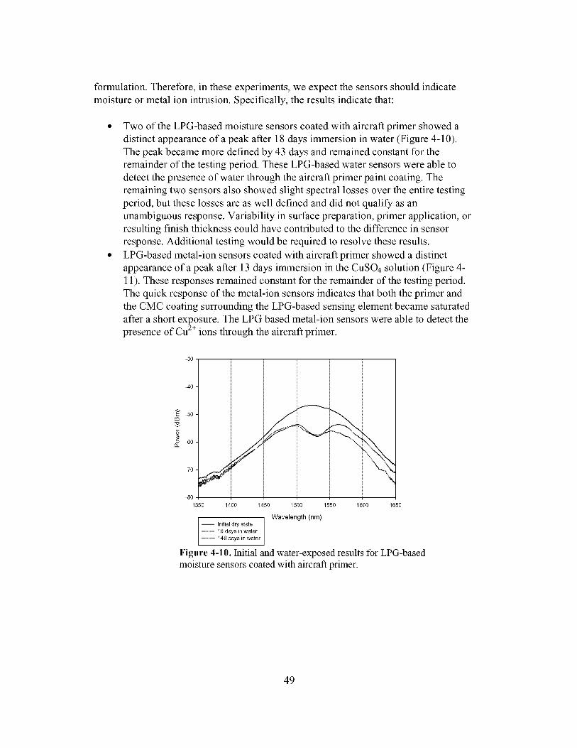
formulation. Therefore, in these experiments, we expect the sensors should indicate
moisture or metal ion intrusion. Specifically, the results indicate that:
• Two of the LPG-based moisture sensors coated with aircraft primer showed a
distinct appearance of a peak after 18 days immersion in water (Figure 4-10).
The peak became more defined by 43 days and remained constant for the
remainder of the testing period. These LPG-based water sensors were able to
detect the presence of water through the aircraft primer paint coating. The
remaining two sensors also showed slight spectral losses over the entire testing
period, but these losses are as well defined and did not qualify as an
unambiguous response. Variability in surface preparation, primer application, or
resulting finish thickness could have contributed to the difference in sensor
response. Additional testing would be required to resolve these results.
• LPG-based metal-ion sensors coated with aircraft primer showed a distinct
appearance of a peak after 13 days immersion in the CuSO4 solution (Figure 4-
11). These responses remained constant for the remainder of the testing period.
The quick response of the metal-ion sensors indicates that both the primer and
the CMC coating surrounding the LPG-based sensing element became saturated
after a short exposure. The LPG based metal-ion sensors were able to detect the
presence of Cu 2÷ ions through the aircraft primer.
-3O
-40 -
E" -50 -rn
o -60 -rl f
-70 -
-80 •
1350 1400 1450 1500 1550 1600 1650
Wavelength (nm)
-- Initial dry state.......... 18 days in water-- 148 days in water
Figure 4-10. Initial and water-exposed results for LPG-basedmoisture sensors coated with aircraft primer.
49

-3O
-4O
E -50
o -600...
-7O
-8O i
1350 1400 1450 1500
Wavelength (nm)-- Initial dry state
-- 13 days in Cu sol.
-- 45 days in Cu sol.
1550
i
1600 1650
Figure 4-11. Initial and CuSO4-exposed results for LPG-basedmetal ion sensors coated with aircraft primer.
Finally, representative plots showing the sensor performance and response compared with
initial conditions are shown in Figures 4-12 and 4-13 for the CPC coated test articles. Theresults indicate that:
• LPG-based moisture sensors coated with CPC showed a broad, shallow dip
after 27 days water exposure, which became slightly more distinct throughout
the remainder of the test (Figure 4-12). Though this dip represents a change in
the optical response through the fiber sensor, it cannot be unambiguously
identified as a spectral loss peak that is indicative of the presence of moisture.
• LPG-based metal-ion sensors coated with CPC showed no change with
immersion in CuSO4 solution for 98 days (Figure 4-13). These results indicate
that the LPG sensing element did not indicate the presence of Cu 2+.
Independent research indicates that the CMC finish is often a quite effective barrier to
short-term intrusion of corrosive environments. Therefore, it is likely that the CMC finish
simply did not allow intrusion of the target molecules through the CMC to reach the LPG
sensor. However, verification of this result would require removal of the finish and an
independent chemical analysis for the presence of the specific constituents be performed.
Overall, the LPG sensors appear promising for detection of incipient corrosion or the
presence of a corrosive environment even beneath characteristic aircraft finishes.
However, these results do indicate that there is an apparent effect on the sensitivity of the
LPG sensor response depending on the thickness of the finish; this must be further
investigated in order to tailor the LPG sensor for a specific finish application.
50

-3O
-4O
-50
}no -60
-70
Er_
v
$o
EL
-8O
1350 1400 1450 1500 1550 1600 1650
Wavelength (nm)-- Initial dry state
-- 27 days in water
-- 202 days in water
Figure 4-12. Initial and water-exposed results for LPG-based moisture sensors coated with CPC.
i
-3O
-4O
-50
-60 _
-70
-80
1350 1400 1450 1500 1550
-- Initial dry state _/avelength (nm)
-- 98 days in copper sol. /Figure 4-13. Initial and CuSO4-exposed results for LPG-based metal ion sensors coated with CPC.
4.2 FATIGUE SENSOR TESTING
4.2.1 Fiber Bragg Grating Sensors
Distributed fiber Bragg grating sensors (Froggatt and Moore 1998) were evaluated for
monitoring fatigue crack growth in a sample designed to simulate a body lap splice. The
purpose of this testing was to establish that an array of distributed Bragg grating sensors
could be used to detect and characterize fatigue cracks by monitoring changes in strain
distribution and signal response signatures.
51

Thelapsplicetestarticleswereconstructedto simulateatypicalaxialfuselagelapjoint.Thesamplehadthreerowsof rivetswith 1-inchspacing.Theinitial EDM(electrostaticdischargemachined)notcheswere0.25inchfromeithersideof aselectedfastenerin thecriticalrow.Theinitial testarticleconfigurationis shownin Figure4-14.
ThreedistributedBragggratingfiberswereattachedto thetestarticlein accordancewiththeproceduresoutlinedbelow.ThegratingsweredistributedandnumberedasshowninFigure4-15.Thesamplewasinstalledin anInstrontestframeattheNASA LangleyResearchCenter'sStructuralTestLaboratoryandsubjectedtoconstantamplitudefatiguecycles(325lbs to 6500lbs; 10Hz).Thecyclingwasstoppedperiodicallysothatstrainsurveyscouldbetakenatminimumandmaximumstaticloads.Cracklengthwasmeasuredusingwide-fieldopticalmicroscopy.Fatiguecyclingwascontinueduntilcatastrophicfailure.(Note:Priorto beginningthetest,it wasdiscoveredthatoneof thesensingfibershadbroken.Thedecisionwasmadeto goaheadwith thetestandignoretheresultsfromthefailedsensors.)
Senso I nst a llati on P eo eed u_e
• Degree} ndelean urfac u in andal 0 0!• Ma_k and miem }a_dbl_f _ing 50 mi_mn A1)O3 _bm}iv_ p_der
. Sp_ayc_a_enti_ teg area N ith M BOnd 600
• Air i0 minu_es morn temperature
• Ra! temperafur to 200{F(Heafing_a{e _F/min; maximum)Cutefo_!hOur
• Clean meba}e_6 urfaceu}ing _l_0h
M_s andmi_6 s andbi_sf{hebasec6a{ su ffieiemlyt remOVe gl a_ed appearaneei
R em 6 _ab _a_i_e P6 _ de_ Ve_idu anS¢ 1_an _im al_0h O1
• P Iace me fib ee n m e _Uefae e _Ueh m a{ m e_{eain _engin g (inde _ed)ar eag _ r {he fiber
a_ein me p_ede_e_in_dl_eafi_ng
ap{ }end6 fib e_ginpla_ep_ *andard p_acti_e
i. Sp aye th enSing fib e_ uSin g M B0 nd 600
NiX e_ 10 minute _ a_ _66m tempemtur_
52

o
o
t_
© ©=oo
,5
1.75"
1.00" _ C rack
© © .-@-/ @ ©
© O O © O
© O O O O
Crack
0.063"_
-0.063"
--0.063"
- (
8 I 0 0
Figure 4-14. Simulated lap splice specimen. A 0.25 EDM cut was maderd
at the indicated fastener (3 fastener from right on top row) to act as acrack starter. The specimen was fabricated from 0.063 in. 2024-T3aluminum sheet.
53

Figure4-15.Bragggrating location and numbering. The gratings marked in red wereignored because the optical fiber was broken prior to the testing.
The data were post-processed using NASA-developed analytical tools (Childers et. al.
2001) to recover individual grating spectra and calculated strains. A typical grating
spectrum is shown in Figure 4-16. Strain was calculated from the change in the
characteristic wavelength (centroid of the grating spectra signal) compared with abaseline value.
0.25
0.20
@
"_ 0.15m
@N= 0.10
Eo 0.05
0.00
Wavelength
Figure 4-16. Typical grating spectrum.
54

Typicalresultsfromthestrainsurveyfor thesensorssurroundingthenotchedfastenerandanadjacentfastenerareshownin Figure4-17.Thedatashowthefractionalincreaseinstrainasthecrackinitiatesfromtheedgeof theEDMnotchandgrowsto,andpast,theadjacentfastener.
Theseresultswereusedto developtestlogicanddiagnosticinferencemodels(DIMs),consistentwith theACAMSapproach,to assessbehaviorsandrelationshipsamongsensorsandtheassociateddamagestate(ARINC2001).Testswereestablishedbyrelatingincreasesinmeasuredstrainto anobserveddamage.Formanyapplications,DIMs canbeexpressedassingleoutcomemodels,eithersupportingor denyingtheexistenceof aparticularfault.However,multi-outcometestswererequiredfor thisapplicationbecausethetestcouldsuggestmorethanonefaultcondition(i.e.,no fault,asmallcrackatanadjacentfastener,alargecrackatanadjacentfastener,alargecrackatadistantfastener,orafailedsensor),dependingonthemagnitudeof thechangein strain.Alist of possiblefaultsthatcouldbesupportedor deniedbyeachBragggratingsensorlocationwasdevelopedfor thesemulti-outcometests.ThedependenciesamongtheseoutcomeswereestablishedandaDIM wascodedandrunonthedevelopmentalACAMSprocessorusingoutcomesderivedfromthefatiguetestresults.Theevidencesupportingtheexistenceof theidentifiedfaultswasaccumulated.TheACAMSprocessorwasableto detectandisolatethefatiguecracksgrowingfromthepre-existingnotchesandwasableto detectwhenthecracksprogressedtothefastenersadjacentto thefasteners.
Furtheranalysisindicatedacorrelationbetweenthetestoutcomesfromthestrain-basedtestsestablishedfor thedependencymodelsandtherecoveredgratingsignals.Representativegratingsignalsandtheircorrelationwith damagestatetestoutcomesfromthedependencymodelareshownin Figure4-18.
Theresultsof theinitial testingof distributedfiberBragggratingstrainsystemindicatethatdistributedstrainsensingcanbeutilizedto detectandcharacterizethedamageresultingfrom structuralfatigueof arealisticstructuralelement.Thefeatureof theBraggsensorthatallowsthesystemtobemassivelymultiplexedofferstheuniquecapabilitytoprovidedetailedstrainmappingthroughoutaregionof interest,suchasthevicinity of thecracktip. Thishassignificantpositiveimplicationsbothfor applicationto SHMwhentheexactlocationof acrackmaynotbeknownapriori, aswell asfor applicationforstructuralcharacterizationunderdamageconditions.Suchquantitativeinformationcanprovidecriticalinformationto aidin anunderstandingof operationalstructuralbehaviors.
Additionaldetailedtestingisunderwayto validatethisapproach,improvetheunderstandingof thetestingvariablesandtheirinfluenceonsensorresponses,andrefinethediagnosticmodels.
55

20
¢-.m
o-
lD
¢-
¢-O
¢-O
.m
O
$..
U_
15
10
5
0
-5
-10
-15
-20
-25
-30
Fastener A6
5000 10000 15000 20000
\\
....... (64) FS
(65) FS
....._----_(66) FS
(72) FS
....._----, (73) FS
(74) FS
10
Cycles
8¢,-
¢,- 4
20')C
0
0-2
C0 -4
0-6
LI_-8
-10
Fastener A5
.ii_i!i,;i; !i!.
_-----;b----- (50) FS 1 ='i_-,,,,,,._ (51) FS &
Cycles
Figure 4-17. Fractional change in strain versus fatigue cycles for gratings
surrounding the notched fastener (top) and an adjacent fastener (bottom). Thestrain increases as the crack approaches the sensor. Large negative changeswere attributed to failure of the sensor fiber.
56

0.25
0.20
=_'_ 0.15
•_ 0.10
Eo 0.05
0.00
0.20
0.18
>, 0.16
0.14
0.12
O.lO•- 0.08
E 0.06
o 0.04
0.02
0.00
ASIGNAL IN ABSENCE OF I_
H
DETICTEI FAULTS/ _,_
wavelength
RGE LOCAL C_,
wavelength
0.20
0.18
0.16
0.14
0.12
O.lO•_ 0.08
E 0.06
o 0.04
0.02
0.00
0.12
>, 0.10
"_ 0.08
-£
0.06
:_ 0.04
c 0.02
0.00
/SMALL LOCAL CRACK J
I
wavelength
wavelength
Figure 4-18. Recovered grating signals and the correlation with damage states.
4.2.2 EFPI Strain and Extensometer Sensor Tests
Test specimens (Figure 4-19) were machined from 0.125 in thick, 2024-T3 aluminum and
7075-T6 sheet with a center notch consisting of an El)M-notched 0.125-in. hole. Strain
gage sensors and extensometers were attached to the center-notched tension specimen as
shown in Figure 4-19. All sensors were oriented parallel to the principal load axis; one
sensor between the notch and the load frame along the centerline of the sample that runs
parallel to the principal loading direction (sensor #6) and the rest distributed along the
centerline perpendicular to the principal load direction (sensors #1-5).
The coupons were subjected to constant amplitude fatigue (load control) until failure in a
MTS fatigue test frame at Penn State University. Load cycles were applied at a frequency
of 10Hz. Every 200 cycles, the cycle rate was reduced to 1Hz for three cycles to allow
strain or crack length measurements to be taken. Because of the high cycling rates and
resulting data rate requirements, strain sensor and extensometer measurements were
accomplished by individual demodulation systems (as described above for EFPI sensors)
and data were captured by the laboratory's data acquisition system. Crack growth was
monitored using a Questar QM100 step zoom long-distance microscope. Digital images
were captured every 6,000-10,000 cycles and crack length was measured from the digital
images.
57

3,0000
p ospo=' '_ 0875 / 0,6850
/
0,8_50
ii_{ s 1,6 50
0
1.00
i _EFPistrainsensor 0,5000_ _,_ 16 _ _0,5000
0,6250 _ I
Figure 4-19. Sample configuration and sensor placement for center crack fatigue
testing. Sensor 1 was an EFPI extensometer. All others were EFPI strain sensors.
All Dimensions in inches
6,5000
The results from fatigue tests of center notched 2024-T3 and 7075-T6 samples are
depicted in representative data in Figure 4-20, 4-21, and 4-22. Figure 4-20 shows strain
measurements from sensors distributed along the likely crack path (i.e., distributed at the
reduced cross-section) and remote from the notch area for 2024-T3 (Figure 4-20a) and
7075-T6 (Figure 4-20b) alloys. These data show a gradual increase in strain resulting
from the reduced sample cross-section as the fatigue crack progresses, followed by a
more rapid increase as the crack impinges on, and passes, the sensors. Figure 4-21 shows
strain measurements from the sensor at the sample centerline parallel to the principal load
axis. These data show a significant decrease in strain as the imposed strain is redistributed
around the growing crack in the later phases of the test. Finally, Figure 4-22 shows the
results from an extensometer placed near the notch of the 7075-T6 sample. These data
show gradual increase in apparent strain (i.e., deflection averaged over the sensor gauge
length) as the crack opens). The extensometer on the 2024-T3 specimen did exhibit this
behavior, indicating that sensor placement near the notch was critical.
58

4500 "
4OOO
3500
3000
.@"_ 2500
2000
1500 "
1000
500 "
45OO
4OOO
35OO
3000
2500
g2000
if)
1500
Strain Sensor #3
Strain at Maximum Load
, f i i i i i.I I I
fI,,,'-"
50,000 100,000 150,000 200,000 250,000 300,000 350,000 400,000 450,000
Fatigue Cycles
lOO0
5OO
0
Strain Sensor #5
Strain at Maximum Load
#
50000 100000 150000 200000 250000 300000 350000 400000 450000
Fatigue Cycles
Figure 4-20a. Results from EFPI strain sensors 3 and 5 (placed along reduced
cross-section remote from notch area) for 2024-T3 specimen.
59

45OO
4000
3500
3000
c
2500o
c 2000
1500
IOO0
500 "
1600
1400
1200
1000
o
•_ 800g
600
4OO
200
10,000 20,000
Strain Sensor #3
l
!/
JI
Strain at Maximum Load "
......... _,_# H_J/
Strain at Minimum Load /
.._...__ .._J _
30,000 40,000 50,000 60,000 70,000
Fatigue Cycles
Strain Sensor #5
/_J
Strain at Maximum Load f_t_
,_ UStrain_
lO,OOO 20,000 30,000 40,000 50,000 60,000 70,000
Fatigue Cycles
Figure 4-20b. Results from EFPI strain sensors 3 and 5 (placed along
reduced cross-section remote from notch area) for 7075-T6 specimen.
80,000
80,000
60

o
._sE
900
800
7OO
600
5OO
400
3OO
200
1 O0
0
- 1 O0
Strain Sensor #6
Strain at MI__ i
Strain at Minimum Load i
50,000 100,000 150,000 200,000 250,000 300,000 350,000 4_ 450 000
Fatigue Cycles
Figure 4-21. Strain vs. fatigue cycles for sensor #6, showing the decrease instrain as the applied load is redistributed around the growing fatigue crack.
8._s
._c
o3
e)
o_
4500
4ooot Ex,ensome,er-Sensor,3500 _ r ....... ----'_"
3000 Apparent Strain at Maximum Load
25OO
2000-
1500-
1000-
5OO
Apparent Strain at Minimum Load
10,000 20,000 30,000 40,000 50,000 60,000 70,000 80,000
Fatigue Cycles
Figure 4-22. Apparent strain vs. fatigue cycles forsensor # 1, showing the crack opening deflection of thegrowing fatigue crack.
61

Thecenter-notchfatiguetestsof EFPIstrainsensorsandextensometersshowedthatthepresenceof growingfatiguecrackscouldbeinferredfrominformationgatheredfromstrategicallyplacedsensors.Thetestresultsprovidedindicationof loadredistributionaroundagrowingdefectbecausethemeasuredstrainswereshownto besensitiveto cracktip position.Althoughtheresultsfrom extensometersweremixed,thereareindicationsthattheycouldprovideaveryimportantmeasureof crackopeningdeflectionthatwouldbehelpfulin monitoringcriticalcrackgrowth.
4.3 TABLETOP SENSOR DEMONSTRATION
In addition to the detailed testing and demonstration of the sensor functionality under
simulated fatigue and corrosion testing, the sensors developed under this program were
demonstrated at the NASA Langley Research Center. These demonstrations, which
occurred July 9-11, 2001, showed:
• The response of the LPG metal ion sensor to various +2 ion solutions. The
sensors were shown to be fully recoverable after exposure to the ion solution.
• The EPFI AE sensor detection of a simulated impact on an aluminum substrate
• Multiplexed EFPI strain sensors using gap division multiplexing
• The LPG moisture sensor response to the presence of water.
In addition, a prototype single Si-chip, multi-microcantilever beam sensor consisting of
three sensing elements and three fiber leads was fabricated for demonstration. The
prototype sensor was demonstrated to monitor wet and dry moisture state, vibration/AE,
and temperature. For the purpose of the demonstration, the sensing elements were
monitored separately by independent demodulation systems.
Finally, in a related demonstration of the ARINC ACAMS capability, the data and sensor
signals from the simulated lap joint fatigue testing described above were used to predict
the behavior of the fatigue crack. In this final demonstration, using ARINC's proprietary
prognostic algorithms, we were able to project the future location of the fatigue crack, on
average, 4000 cycles prior to the actual propagation (ARINC 2001).
4.4 SENSOR SYSTEM IMPLEMENTATION CONSIDERATIONS
This section has summarized the sensor system testing for application to SHM. The
results show that structural degradation of aircraft materials can be effectively detected
and characterized using available sensors. As was described in the previous section,
implementation of SHM systems will require the fusion of information from arrays of
multiple sensor types acting in concert. Therefore, the ability to multiplex sensors and to
combine different sensors into a coherent system is crucial to any future implementation.
62

Table4-2presentsasummaryof the integrationcapabilitiesfor thefiberopticsensortechnologiesdevelopedor evaluatedunderthisprogram.Thefiberopticsensorsevaluatedin thisprojectoperateononeof threewavelengths--830nm,1300nm,and1550nm.Eachsensortechnologyutilizesaseparatebandandthereforeadifferenttransmissionfiber.As aresult,in thecurrentstateof sensortechnologymultiplesensortypescannotbemultiplexedonasingleopticalfiber.
Table4-2. Summaryof CurrentFiberOpticSensorTechnologySensor Wavelength Multiplexing System CommentsTechnology Refresh
Rate
EFPI Strain 830nm 1 Hz Using 1 Fiberscan + 1 Mux 88 channels, switched(see Note 1)
4 channels, in-line 15 Hz Using 1 Fiberscan, in-linemultiplexing
1 channel 60 Hz Using 1 Fiberscan
Acoustic 1300nm 1 channel 400 kHz Using 1 single-channel FOSSEmission NDE system
LPG 1550nm 1 Hz Using 1 Lunascan + 1 Mux 8Corrosion
8 channels, switched(see Note 1)
3 channels, in-line 30 Hz Using 1 Lunascan, in-linemultiplexing
1 channel 100 Hz Using 1 Lunascan
Note 1 lx8 switched mutiplexors can be cascaded in arrangementsup to 64 sensors
The EFPI strain technology operates at 830nm source/fiber. Multiplexing of EFPI strain
sensors can be achieved in two ways: 1) optical switching and 2) in-line multiplexing.
Optical switching uses a MEMS device to circuit switch between fiber legs each having
up to 8 sensors, polling each of these sensors using a single demodulation system in a
round-robin fashion. Gap division multiplexing (GDM) can be used to provide serial, in-
line multiplexing (i.e., placing more than one sensor on a single optical fiber) of EFPI
strain sensors. Up to 4 EFPI sensors can be multiplexed using this technique. While a
significant system cost saving per channel can be realized by multiplexing the number of
sensors that share sources and demodulation systems, each multiplexing techniques
degrades the system performance by reducing bandwidth in proportion to the number of
multiplexed sensors.
The EFPI acoustic emission technology utilizes 1300 nm source/fiber and does not
currently lend itself to multiplexing. As described earlier in this section, the EFPI AE
sensor technology is based on an intensity system, which allows only one sensor per
channel (or per fiber).
63

ThecorrosionsensortechnologyisbasedontheLPGconceptandusesa 1550nmsourceandfiber.Like theEFPItechnologies,thesesensorscanbemultiplexedthroughopticalswitchingandin-linemultiplexing.Thecurrentin-linemultiplexingcapabilityis limitedto 3 sensors.As with theEFPIstrainsystem,reductioninbandwidthisproportionalto thenumberof multiplexedchannels.
ThedistributedBragggratingstrainsystemiscapableof measuringalargenumberofsensors(potentially,up to 10,000strainsensors)alongasingleopticalfiber,witha singledemodulationsystem.Thismultiplexingcapabilityresultsin thelowestprojectedsystemcost.
Althoughtherearenumerousbenefitsto spectralinterrogationsystemsusedin theEFPIandLPGtechnologies,therearesomeaspectsof thedesignthateffectmeasurementsinflight environments.Onesignificantdrawbackis thespeedof thesystem,whichis atleastthreeordersof magnitudeslowerthanrelativeinterrogationsystems(~100Hzcomparedto >1MHz). Thesourceof theproblemis thespeedof thespectrometerinternalto thesystem,whichusesaCCDarraytomeasuretheintensitiesof thewavelengths.Althoughthis is aproblemin manyapplicationswhereeventsoccurfasterthan100Hz, anduptohundredsof kilohertz,thekineticsof low-cyclefatigueandcorrosionprocessesoncommercialaircraftmakeit unlikelythatthesystemspeedwill becomeanimplementationconcernfor themajorityof applications.
Sensorsystemhardwareconsiderationsalsoneedtobeconsideredin aneventualimplementation.Thehardwarerequirementsincludeaminiaturespectrometer,aDSPprocessorcard(DSP,peripheralcomponents,A/D circuitry,etc.),andalaserdiodesourcefor eachsystem.Currently,thelight sourceandopticalcomponenttechnologiesarebasedonavailableoff-the-shelfcomponentsandarelimitedin theirtemperaturetoleranceandsensitivity.In thepast,thermo-electriccoolershavebeenusedto compensatefor thetemperatureextremesin serviceapplications.
64

SECTION 5SENSOR DATA INTERPRETATION
5.0 INTRODUCTION
A key component of the structural health monitoring capability is the ability to interpret
the information provided by sensor system to characterize the structural condition. The
diagnostic inference models described for the lap splice testing in the previous section
represent one method for relating sensor outcomes to potential faults to assess the state of
structural health. Physical models are another tool that will be required to establish
system structural health and to project how structural degradation will likely progress.
This section describes a deterministic state-space fatigue growth model and stochastic
model that accounts for the statistical nature of damage development processes. These
models were developed to perform real-time characterization and assessment of structural
fatigue damage.
5.1 STATE-SPACE MODEL OF FATIGUE CRACK GROWTH
Modeling of fatigue crack growth has been a topic of intensive research for several
decades. Based on different experimental data, many models (e.g., Anderson 1995,
Bannantine et al. 1990, Suresh 1991) have been proposed for fatigue life prediction.
Fatigue crack growth models have been used for damage mitigating control of complex
mechanical structures such as aircraft (Ray and Caplin 2000), rocket engines (Dai and
Ray 1996; Holmes and Ray 1998), and power plants (Kallappa et al. 1997; Holmes and
Ray 2001).
Modeling of fatigue crack growth under variable-amplitude loading usually relies on a
memory-dependent physical variable (e.g., crack opening stress, or reference stress) that
requires storage of information on the load history. In current state of the art of fatigue
crack growth modeling, the finite interval over which the load history is considered to be
relevant may vary with the type of loading as well as with the rules employed for cycle
counting. Nevertheless, this memory-dependent variable can be modeled in a finite-
dimensional state-space setting by an ordinary difference (or differential) equation. The
complete information on the state at the current cycle is realized as a combination of the
partial information on the state and the history of the input (i.e., cyclic stress) excitation at
finitely many previous cycles.
The state-space model is a nonlinear dynamical model of fatigue-crack growth under
variable-amplitude loading in ductile alloys following the state-space approach (Patankar
and Ray 2000). The crack growth equation in the state-space model is structurally similar
to Paris equation (Paris and Erdogan 1960) modified for crack closure, which has been
extensively used in fatigue crack growth models such as FASTRAN (Newman 1992) and
AFGROW (Harter 1999). Under variable-amplitude loading, these models usually rely on
a memory-dependent physical variable (e.g., crack opening stress or reference stress) that
requires storage of information on the load history. For example, the crack-opening stress
65

in theFASTRANmodel(Newman1992)isassumedto dependontheloadhistoryoveranintervalof about300cycles.Anotherexampleis thestrain-lifemodelin whichthereferencestressobtainedbytherainflowmethodreliesoncyclecountingthat,in turn,dependsontheloadhistory(DoMing 1983).Themodelpredictions,in general,becomemoreaccurateif theloadhistoryisconsideredovera longerperiod,althoughashortrecenthistoryof theappliedloadmightbeadequatein somecasesforcrackgrowthmodeling.An extremeexampleis constant-amplitudecyclicloadingwherestorageof theloadhistoryoverthepreviouscyclesmaynotbenecessary.It isnotpreciselyknowntowhatextentinformationstorageis necessaryfor calculatingthememory-dependentvariablein afatiguecrackgrowthmodelundera priori unknown variable-amplitude
(e.g., single-cycle, block, spectrum, or random) loading. The state at the current cycle is
realized as a combination of the state and the input (i.e., cyclic stress) excitation at
finitely many previous cycles. Equivalently, the state becomes a function of the fading
memory of the input excitation, which can be generalized to an autoregressive moving
average (ARMA) model that is equivalent to a state-space model (Ljung 1999). Unlike
the existing crack growth models, the state-space model does not require a long history of
stress excitation to calculate the crack-opening stress. Therefore, savings in the
computation time and memory requirements are significant.
Although the structure of the state-space model's crack growth equation is similar to that
of FASTRAN (Newman 1992), it adopts a novel approach to generate the (cycle-
dependent) crack opening stress under variable-amplitude loading. As such, the crack
length computed by these two models could be different for given variable-amplitude
loadings, even though the results are nearly identical under the same constant-amplitude
loading.
The state-space model was formulated to satisfy the following requirements:
• Capability to capture the effects of single-cycle overload and underload, load
sequencing, and spectrum loading
• Representation of physical phenomena of fracture mechanics within a semi-
empirical structure
• Compatibility with plant dynamic models for health management and life
extending control
• Validation by comparison with fatigue test data and a well known code of fatigue
crack growth
• Computer code development for real-time execution on standard platforms
The first two requirements were satisfied as the state-space model was formulated based
on fracture-mechanistic principles of the crack closure concept. The third requirement
was also satisfied because the plant dynamic models are usually formulated in the state-
space setting or autoregressive moving average (ARMA) setting (Ljung 1999). The
remaining two requirements were satisfied by validating the state-space model with
fatigue test data for different types of variable-amplitude and spectrum loading on 7075-
T6 and 2024-T3 alloys (Porter 1972; McMillan and Pelloux 1967). The model predictions
66

werealsocomparedwith thoseof AFGROWandFASTRAN,whicharewell-knowncodesfor fatiguecrackgrowthpredictionthatarewidelyusedin theaircraftindustry.
5.1.1 State-Space Model Formulation
5.1.1.1 Nomenclature
Ajk
a
cE
F(*,*)
h(o)
k
m
m
n
R
sflOW
smax
smin
S °
S 05'5'
sUlt
S y
t
U(o)
W
O_
O_ max
O_min
Aa max
Aa min
Aak
AKeff
6thr
parameter in the empirical equation of S_ss for j = 1,2, 3, 4
crack length
parameter in the crack growth equation
Young' s modulus
crack length dependent geometry factor
crack growth function in crack growth equation
current cycle of applied stress
exponent parameter in the crack growth equation
number of cycles of a particular stress level in the load block
number of cycles of a particular stress level in the load blockstress ratio of minimum stress to maximum stress
flow stress
maximum stress within a cycle
minimum stress within a cycle
crack opening stress
crack opening stress under constant amplitude load given by empirical equation.
ultimate tensile strength
yield stress
specimen thicknessthe Heaviside function
half-width of center-cracked specimen or width of compact specimen
constraint factor for plane stress/strain
maximum value of
minimum value of
crack increment above which a = 6¢min
crack increment below which a = 6¢max
crack increment (= ak - ak-1)
effective stress intensity factor range
positive lower bound for absolute value of maximum stress lS_nax, k _>0 l"/
decay rate for S °
5.1.1.2 Model Development
The state-space model was formulated based on the crack closure concept where the state
variables are the crack length a and the crack-opening stress S ° . A difference equation
67

for $2 has been constructed in such a way that, under different levels of constant
amplitude load, the forcing function S°k_'_'at the k th cycle matches the crack opening stress
derived from the empirical relation (Newman 1984) given as:
where
oss
Sk
A_ = {Io-A°-A_k-A3
: s °__(sF x,sF, ak,F(ck_l,w))
I(max{(A°+ A_R_+ £R_ 2+ A3Rg),R _,,_k....,R__>00 1 max •
[(A k + AkR k)S k ,otherwise(SS-1)
Rk _ S_ _ U(Skm_x) for all k > 0 (SS-2)Sk
0 (SS-3)A k = (0.825-0.34a k +0.05ak 2) cos SYOW )]
sFx F(c___,w)(0"415 - 0"071ak)
if R k -> 0
if R k -< 0
(SS-4)
(ss-5)
20A° A 1-1 ifR k>0A3 = x + x
k if R k -< 0(SS-6)
The following constitutive relation in the form of a piecewise bilinear first order
difference equation has been proposed (Patankar and Ray 2000) for recursive
computation of the crack opening stress S[ at the completion of the (k-l) th cycle:
68

f _
"[- [_J --g(Sk --Sk_l)_-_(Sk_i1 l -sknill1S k -S°sS(Sk ,Sk_l) ]
(ss-7)
_S y
where 7/ (SS-8)2wE
{_ if x<_OThe Heaviside function U(x) = if x > 0
and the forcing function S2_'_'is calculated from the semi empirical formula given by Eq.
(SS-1) as if constant amplitude stress cycles (STx,s_ 1) were applied.
S2_'_'generated from the semi-empirical Eq. (SS-1) is used to construct the (piecewise
bilinear) forcing function to the dynamics of crack opening stress $2 in Eq. (SS-7). Under
constant amplitude stress excitation, S °_'_'is the steady state solution of S ° . However,
under variable amplitude stress excitation, S__'_'is different from the instantaneous crack
opening stress $2.
Following an overload cycle, the duration of crack retardation is controlled by the
dynamics of S ° in the state-space model, and hence determined by the stress independent
parameter rI defined in equation (SS-8).
The last term on the right hand side of Eq. (SS-7) accounts for the effects of reverse
plastic flow. The overload condition and the reverse plastic flow condition are mutually
exclusive. The former feature is mathematically represented by the Heaviside function
U(S; ss - S;_ 1 ) in the third term on the right hand side of Eq. (SS-7). Moreover, depletion
of the normal plastic zone occurs when an underload occurs. The underload effects have
been incorporated via another Heaviside function U(Sk_'I _ - S__).
5.1.1.3 Prediction of Sequence Effects
Figure 5-1 shows the effects of a single cycle overload on S ° , as predicted by the state-
space model in Eq. (SS-7). The model predictions are qualitatively similar to the
experimental data of Yisheng and Schijve (1995) except for the lack of a sharp negative
spike in S ° immediately after the application of an overload. The sharp transients of S °
that occur only for a few cycles have no significant bearing on the overall crack growth.
69
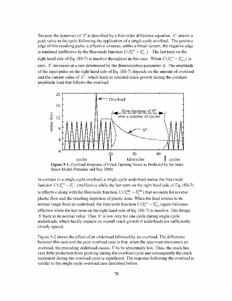
Becausethedynamicsof S ° is described by a first order difference equation, S ° attains a
peak value in the cycle following the application of a single cycle overload. The positive
edge of this resulting pulse is effective whereas, unlike a linear system, the negative edge
is rendered ineffective by the Heaviside function U(S°k _'_'- Sk°_l). The last term on the
right hand side of Eq. (SS-7) is inactive throughout in this case. When U(S°k _'_'- Sk°__) is
zero, S ° decreases at a rate determined by the dimensionless parameter 7/. The amplitude
of the input pulse on the right hand side of Eq. (SS-7) depends on the amount of overload
and the current value of S ° , which leads to retarded crack growth during the constant
amplitude load that follows the overload.
20
16
12r_
r_
O
._ 8r_
Overload
s #
30 40
cycles kilocycles I cycles
,;'4 Slow decrease of S° - ,.......... -_,over a number of cycles ,
t[_ll, II
\ ............ \\ ...... SO \
/
20
I
1t
Figure 5-1. Overload Response of Crack Opening Stress as Predicted by the State-Space Model (Patankar and Ray 2000).
In contrast to a single cycle overload, a single cycle underload makes the Heaviside
function U(S°k _'_'- Sk°_l) ineffective while the last term on the right hand side of Eq. (SS-7)
is effective along with the Heaviside function U(Sk__I1 - S_ _) that accounts for reverse
plastic flow and the resulting depletion of plastic zone. When the load returns to its
normal range from an underload, the Heaviside function U(S°k _'_'- Sk°_l)again becomes
effective while the last term on the right hand side of Eq. (SS-7) is inactive. This brings
S ° back to its normal value. Thus S ° is low only for one cycle during single cycle
underloads, which hardly impacts on overall crack growth if underloads are sufficiently
closely spaced.
Figure 5-2 shows the effect of an underload followed by an overload. The difference
between this case and the pure overload case is that, when the specimen encounters an
overload, the preceding underload causes S ° to be abnormally low. Thus, the crack has
very little protection from growing during the overload cycle and consequently the crack
increment during the overload cycle is significant. The response following the overload is
similar to the single cycle overload case described before.
70

2oI15
Overload
o •
; _ Sl__ow.decrease 9[ _S. "1_ !.. Over a number of cycles
'..........10I %., I
I "',.,... O I I
;: ................ ,,
0
-520 30 40
cycles I kilocycles I cycles
Figure 5-2. Underload-Overload Response of Crack Opening Stress as Predicted
by the State-Space Model (Patankar and Ray 2000)
Figure 5-3 shows how S ° is affected by an overload immediately followed by an
underload. In the overload-underload cycle, $2 l_xis identical to that for pure overload but
the corresponding _1 • o_,_,S k is smaller. Consequently, S k is smaller for overload-underload
than that for a single cycle overload. In effect, the forcing function that is multiplied by
the Heaviside function U(S2 _'_'-Sk°_l )in Eq. (SS-7) assumes a smaller value for overload-
underload than that for a single cycle overload, while the last term on the right hand side
of Eq. (SS-7) is inactive. A single cycle overload retards crack growth more effectively
than a similar overload immediately followed by an underload. Thus the benefits of an
overload monotonically diminish with increase in the magnitude of the followingunderload.
20
15
f-%
_10
0
5r¢?
0
-5
Underloa8-----_
Overload
OSlow decrease of S - ,_1- ........... ----I_ ,,
, over a number of cymes ,
" . \AAh,,,,....................... !, ........................................................>.._._,_
i /I/77
i i i
20 30 40
cycles I kilocycles I cycles
Figure 5-3. Overload-Underload Response of Crack Opening Stress asPredicted by the State-Space Model (Patankar and Ray 2000).
71

5.1.2 Model Validation with Test Data
The state-space model has been validated with the fatigue test data of: (1) 7075-T6
aluminum alloy specimens under different types of variable amplitude cyclic loading
(Porter 1972); and (2) 2024-T3 aluminum alloy specimens under spectrum loading
(McMillan and Pelloux 1967), which are available in open literature. The state-space
model predictions have been compared with those of FASTRAN (Newman 1992) and
several other crack-tip-plastic-zone-based models (e.g., Wheeler, Willenborg, and Chang)
that are available in the AFGROW software package (Harter, 1999). On all the
AFGROW models, predictions of the Walker equation with Willenborg retardation model
were found to yield, on the average, closest agreement with the test data of McMillan and
Pelloux as well as Porter. The complete set of validation comparisons (Sastry 2000) is
presented in Appendix A. The results are summarized below.
Porter (1972) collected fatigue test data on center-notched 7075-T6 aluminum alloy
specimens made of 305 mm wide, 915 mm long, and 4.1 mm thick panels, for which
E = 69600 MPa, (yY= 520 MPa, and o-"lt = 575 MPa. The initial crack size (2a) was 12.7 mm
and the experiments were conducted in laboratory air. The profile of block loading for
data generation is shown at the top of Figures 5-4 and 5-5 where the positive integers, n
and m, indicate that a block of n constant-amplitude cycles is followed by a block of m
cycles of a different constant-amplitude.
Figures 5-4 and 5-5 show comparisons of the state-space model predictions with Porter
data and the predictions of FASTRAN model and AFGROW (Walker equation with
Willenborg retardation model) that calculate the crack opening stress in a different way.
The analyses on each of FASTRAN, AFGROW, and the state-space models have been
conducted with identical initial crack length with the assumption of no loading history.
The curves in Figure 5-4 are generated with the parameters n = 50 and m = 1 with
different values of the overload G2 and underload G1 superimposed on constant-
amplitude stress cycles of 103.43 MPa and 51.72 MPa for repeated overload-underload
spectra. Similarly, the curves in Figure 4-5 are generated with the parameters n -- 50 and
m -- 1 with different values of the overload G2 and underload G1 superimposed on
constant-amplitude stress cycles of 103.43 MPa and 51.72 MPa for repeated underload-
overload spectra.
The state-space and FASTRAN models produce nearly identical results under constant-
amplitude cyclic stresses, because the procedure for calculating S °ss is similar in both
models while the AFGROW model yields somewhat different results. For variable-
amplitude cyclic stresses, the state-space model predictions are quite close to both the
experimental data and predictions of the FASTRAN model, as seen in Figures 5-4 and
5-5. These plots indicate that the accuracy of the state-space model relative to the
experimental data is comparable to that of the FASTRAN model. On the average, for
repeated overload and underload, accuracy of the state-space model is comparable to that
of FASTRAN and AFGROW. The results show that the state-space model (and, to lesser
extent, FASTRAN) demonstrates the difference between the effects of overload-
72

underloadandunderload-overloadoncrackgrowthin agreementwith thetestdata.Incontrast,theAFGROWmodeldoesnotshowanyappreciabledifferencewhencorrespondingresultsarecompared.Thepredictionsof thestate-spacemodelareapparentlysuperiorto thoseof AFGROWfor sequenceeffects.
9O
80
¢ 70E
60g-1- 50
40Zill-_ 30
o 20<r,fo 10
g_ lO3.43 7---- ,',----" ,',
r._ 51.72 , , --11--50cy cles II
O1 "1 cycle---P'_41--_l_J
00 20 40 60 80 100 120
KILOCYCLES
100
90
¢ 80
E= 70
g 60I
50,,z4oiJ
3o<r_ 2OO
10
00
................ AFGROW
120.......... Fastran l! ....
StateSpace ii.. No overload
¢ 100 _ ] ] Only mlderload_ Porter Data
_ 80 ............... AFGROW I..L.. m=l, n = 50E L _ _ " .." T .."
z_ 60 (51=5"17MPa] "'" i/(]2 =103.43 MPa] _''" /i
-J 40x_
o_ 20
00 10 20 30 40 50 60 70 80 90
KILOCYCLES
90
80 ...........
_)
"_ 70
60 ................... AFGROW
50
40,," 3O
r_ 2OO
10
00 20 40 60 80 100 120
KILOCYCLES
70 .... i _ i......... Fastran I Iil I
i /,I
_5o17 MPa I
StateSpac4.i-i-t % I""¢...._'¢ 60 ----*--- Porter Data Ii ii _2 =206.85 MPal/
................AFGROW "'|.,L.i._..........'-...........s...........i ..........."-'_........so
_ ti,i i iir4o ....i......i...i...........i..........i...........i....../i.........."- i'i i i i/iz_ 30 ............:...........i...........i.........._-4.-.-.-i..........._...........L-.-7_L-.---4..........
i i i ii i i i / i i_, i i i Y i i o,.-i" i i
<°" olo 1 i i Z20 40 60 80 100 120 00 1'0 20 30 a_0 50 60 70 80 90 100
KILOCYCLES KILOCYCLES
Figure 5-4. Comparison of analytic model predictions with published overload-
underload) fatigue data. Data source: Porter 1972.
73

o 2
_" 1 cycle103.43 ....
v!A/4= .L,J_ __51.73
50 cycles
O 1
90
_8o_7o
_6oZ5o(.9,,z,4o
530_2oo
10
.......... Fastran
State Space
0 20 40 60 80
KILOCYCLES
100
.................AFGROW
(J2 =155.14
0 50 100 150KILOCYCLES
100
90
80d)
E 70
g 60"1-
_ 5o,,z4o
x: 3Oo_<2oo
10
70
60
._ 50
E_-4o
z_ 3oW
_ 2o<_1o
0 00 20 40 60 80 100 120 140
KILOCYCLES
i ---...... i
.....I-.,-_-,,,,,,,_'-"""_'--A?_roDv_/ta t.............i ............7.{...
(51=5.17 MPa ................._"j
"'_Ziiiii'iiiii'l1_2 =206i851111ii)ii!i'i!i!ii:.iii'[':_ "_ "'"MPal ..............._"..................
20 40 60 80 100 120KILOCYCLES
Figure 5-5. Comparison of analytic model predictions with published overload-
underload) fatigue data. Data source: Porter 1972.
McMillan and Pelloux (1967) generated fatigue data under complex spectrum loads for
center-notched 2024-T3 aluminum alloy specimens made of 229 mm wide, 610 mm long,
and 4.1 mm thick panels. Fatigue testing was accomplished in a vertical 125 kip electro-
hydraulic fracture jig of Boeing design. The testing system was capable of applying loads
with an absolute error within _+1% of the maximum programmed load. The initial crack
size (2a) was 12.7 mm and the experiments were conducted in laboratory air.
Figure 5-6 shows predictions of the state-space, FASTRAN, and AFGROW models with
selected four of the thirteen spectral data sets of McMillan and Pelloux. The state-space
model predictions are closest to the experimental data in twelve out of the thirteen cases
of spectrum loads except for the data set P 10.
74

r4 t _ _ _ ,,. _,llsrrm192o
,.@10
__ 7 _ _ I 2 3 4 _ 11517181920
YvlYVY'-'"......I 123_.2
Program P9 One block of loading
4.0
I
I0 I
e_l0 12i_ 14_5_e
....° II" I'l'q
_ar9 _o
12
Program PlO One block of loading
2
g"1-
(9z
0
0
80Fastran
70State Space
60 Test Data
50 ...................... AFGROW
4O
3O
0 o 20 40 60 80 100 120 140 160 180
KILOCYCLES
80.......... Fastran
70 _ State Space
60 _ Test Data -_................ AFGROW J50
40 //30
-/S "J2o10
0
m/
0 20 40 60 80 100 120 140
KILOCYCLES
14
12
# 7
I 2 _ 4
I|1"_I_1"¼1SltlTlillil_'l t Z 3 15 II 7 I191_,1
Program P11 One block of loading
20 40 60 80 100 120 140 160 180 200
KILOCYCLES
14
c./3
5
. _ 2 3 8 S IO II 12: IS)20
I 2 $ 4 ll; 1718 19 _0 I °
Program P13 One block of loading o o 20
%" 80 Fastran
70E
60 Test DataE
_'5o40
z
w, 30
20_0O
40 60 80 100
KILOCYCLES
Figure 5-6. Comparison of analytic model predictions with published spectrum
fatigue data. Data source: McMillan and Pelloux 1967.
120
75

Modest disagreements (in the range of approximately 10%) between the state-space
model predictions and the test data are reasonable because the number of samples (e.g., in
the order of three or four) over which the test data are averaged is small. The agreement
of model predictions with experimental data strongly supports the state-space model and
its fundamental hypothesis that the crack opening stress can be treated as a state variable.
5.1.3 Comparison of Computation Time
Table 5-1 and Table 5-2 list typical computation time required for calculation of crackgrowth under programmed loads for Porter data and McMillan and Pelloux data,
respectively, on a 450 MHz Intel Pentium PC platform. In the thirteen cases reported in
Table 5-2, the state-space model predicts a longer life than FASTRAN by a few thousand
cycles. In the case of spectrum P 10, both models run for approximately the same number
of cycles which provides a fair comparison of their computation time. The execution time
per spectrum block for both the models indicates that the state-space model is about 10
times faster than FASTRAN for each of the thirteen spectrum load cases.
Table 5-1. Execution Time for Overload-Underload Cases
Repeated Load Blocks(N cycles @ 68.95 Mpa;1 cycle @ 103.43 MpaMin. stress 3.45 Mpa)
Time in Secondson a 450 Mhz PentiumState-SpaceModel
FASTRANModel
N=1000 1.20 4.80N=300 1.10 4.50N=50 0.50 2.30
Table 5-2. Execution Time for Spectrum Load CasesLoad State-Space Model FASTRAN ModelDescription (Time in Seconds) (Time in Seconds)
Program P1 0.65 4.09Program P2 0.69 4.55Program P3 0.50 5.70Program P4 0.48 4.10Program P5 0.47 5.07Program P6 1.17 5.51Program P7 1.28 5.10Program P8 0.97 6.41Program P9 0.79 7.16Program P10 0.50 5.60Program Pll 1.07 5.36Program P12 0.64 6.53Program P13 0.66 5.31
76

The state-space model recursively computes the crack opening stress as a state variable as
a simple algebraic function of the maximum and minimum stress excitation in the present
cycle as well as the minimum stress and the crack opening stress in the immediately
preceding cycle. In contrast, the FASTRAN model computes the crack opening stress as a
function of contact stresses and crack opening displacements based on the stress history.
Since the state-space model does not need storage of load history except the minimum
stress in the previous cycle, the memory requirements are much lower than those of
FASTRAN that does require storage of a relatively long load history. Consequently, both
computer execution time and memory requirement of the state-space model are
significantly smaller than those of the FASTRAN model. Specifically, the state-space
enjoys the following advantages over other crack growth models:
Smaller execution time and computer memory requirements as needed for real-
time heath management and life extending control (Holmes and Ray 1998)
Compatibility with other state-space models of plant dynamics (e.g., aircraft
flight dynamic systems and rocket engine systems) and structural dynamics of
critical components as needed for synthesis of life-extending control systems
(Holmes and Ray 1998)
5.2 STOCHASTIC MODELING OF FATIGUE CRACK DAMAGE
Traditionally, the risk index and remaining service life (Bolotin 1989) of machinery are
calculated off-line based on statistical models of material degradation, operating history,
and anticipated disruptions in the plant operation (e.g., postulated stress levels). Because
the predicted service life of operating machinery is likely to be altered in the event of
unscheduled operations, on-line computation of damage statistics allows continual
refinement of the risk index and remaining life prediction as time progresses. In this
context, this report focuses on stochastic modeling of fatigue crack damage in metallic
materials, which is a major source of failures in structural components of operating
machinery (Ozekici 1996).
Stochastic modeling of fatigue crack phenomena in ductile alloys is a relatively new area
of research, and a list of the literature representing the state of the art is cited by Sobczyk
and Spencer (1992) as well as in the March 1996 issue of Engineering Fracture
Mechanics. Bogdonoff and Kozin (1985) proposed a Poisson-like independent-increment
jump model of fatigue crack phenomena. The underlying principle of this model agrees
with the theory of micro-level fatigue cracking. An alternative approach to stochastic
modeling of fatigue crack damage is to randomize the coefficients of an existing
deterministic model to represent material inhomogeneity (Ditlevsen 1986). Another
alternative approach is to augment a deterministic model of fatigue crack growth with a
random process (e.g., Lin and Yang 1985; Spencer et al. 1989; Ishikawa et al. 1993). The
fatigue crack growth process is thus modeled by nonlinear stochastic differential
equations in the It6 setting (Kloeden and Platen 1995). Specifically, Kolmogorov forward
and backward diffusion equations, which require solutions of nonlinear partial differential
equations, have been proposed to generate the statistical information required for risk
77

analysisof mechanicalstructures(TsuruiandIshikawa1986;Bolotin1989).Thesenonlinearpartialdifferentialequationscanonlybesolvednumericallyandthenumericalproceduresarecomputationallyintensiveastheyrelyonfine-meshmodelsusingfinite-elementorcombinedfinite-differenceandfinite-elementmethods(SobczykandSpencer1992).Casciatiet al. (1992) have analytically approximated the solution of It8 equations
by Hermite moments to generate a probability distribution function of the crack length.
Formulation and assessment of a stochastic model of fatigue crack damage in ductile
alloys that are commonly encountered in aircraft structures is presented in the following
subsections. The fatigue crack damage at an instant (i.e., at the end of a stress cycle) is
expressed as a continuous function of the current and initial crack lengths. The (non-
stationary) probability distribution of crack damage is obtained in a closed form without
numerically solving stochastic differential equations in the Wiener integral or It8 integral
setting. Model predictions are shown to be in close agreement with the fatigue test data of
2024-T3 and 7075-T6 aluminum alloys. Finally, an illustration is provided to describe
how the stochastic model can be used in making decisions for risk analysis and life
prediction that are necessary for health management and life extending control of
mechanical systems.
5.2.1 Model Formulation and Assessment
5.2.1.1 Nomenclature
C autocovariance; covariance matrix
C crack length
7M critical crack length
7o threshold of initial crack length
F(.) probability distribution function
f final condition
H hypothesis
K stress intensity factor
M number of hypotheses
m exponent parameter of the model
O initial condition; opening condition
p[.] probability measure
R stress ratio (smin/smax); autocorrelationS stress
T maximum time of operation
t time (cycles)X random vector
x random variable
Yd desired operational profile
A incremental range
8 increment operator
8(.) unit impulse function
e confidence level for risk analysis
_) eigenvector
dummy variable
A (diagonal) eigenvalue matrix
)_ eigenvalue
_t expected value
p multiplicative white noise
standard deviation
_c dummy variable
_' discretized fatigue crack damage
continuous fatigue crack damage
multiplicative parameter of themodel
sample point (test specimen)
78

5.2.1.2 Modeling of Fatigue Crack Damage
Fatigue crack growth models have been formulated by fitting estimated mean values of
fatigue crack length, generated from ensemble averages of experimental data, as functions
of time in units of cycles (Paris and Erdogan 1963; Schjive 1976). Following Sobczyk
and Spencer (1992) and the pertinent references cited therein, the stochastic model of
fatigue crack damage presented in this report, is built on the structure of the following
mean-value model (Anderson 1995; Suresh, 1991):
8_(t) = h(AKef f (t)) St; for t _>t o and given _(t o)
AKef f (t) = AS(t)_ F(8(t))
AS(t) = S max (t) - S ° (t)
where t is the current time upon completion of a stress cycle, to is the initial time (e.g.,
when the machine component is put in service after a major maintenance or inspection),
_(t) is the estimated mean value of (time-dependent) crack length, 8_(t) is the increment
of the estimated mean crack length over one cycle after time t, 8t indicates the time
increment over that cycle, h(o) is a non-negative continuous function that is dependent on
the material and geometry of the stressed component, and AS(t) is the effective stress
range during one cycle (after time t) with the corresponding crack opening stress S° (t)
and peak stress Smax (t). The (dimensionless) correction factor F is dependent on
geometrical configuration (e.g., thickness, width, and the crack type in the stressed
component) and the crack length. For example, F = 1/sec(_ 8(t)/(2w)) for center-cracked
specimens of half-width w. There are several empirical and semi-empirical methods
(e.g., Newman 1984) for calculating S° . For constant-amplitude load, Ibrahim et al.
(1986) formulated a simple algebraic relation to obtain S° as a function of peak stress
Smax and stress ratio t{ _--S min /S max .
It has been shown that for a given geometry (i.e., thickness and width) of center-cracked
specimens, the function h(o) can be expressed as a product of two functions, h 1 (AS(t))
and h 2 (8(t)) (Anderson 1995; Suresh 1991). Accordingly, for center-cracked specimens
with 0 < 8(t) < w Vt _>to, Eq. (1) is modified via series approximation of the (m/2) th power
of the secant term in the correction factor F as:
;t)to d iven (to)where the constant parameters fi and m are dependent on the specimen material,
geometry, and fabrication. For constant-amplitude load, Eq. (2) reduces to the well-
known Paris equation (Suresh 1991). For varying-amplitude load, Patankar and Ray
(1)
(2)
79

(2000) have shown the validity of Eq. (2) under time-dependent stress range
AS(t) --- (Smax(t) - S ° (t)) by having S° (t) as a state variable.
Ditlevsen (1986) has shown that, under constant load amplitude the randomness of
fatigue crack growth accrues primarily from parametric uncertainties. The stochastic
process of crack growth is largely dependent on two second-order random parameters--a
multiplicative process _(4,AS) and an exponent parameter m(4). Ditlevsen (1986) has
suggested the possibility of one of the above two random variables being a constant for
all specimens 4. Statistical analysis of the experimental data for 2024-T3 and 7075-T6
aluminum alloys reveals that the random exponent m(4) can be approximated as a
constant for all specimens (i.e., m(4) = in with probability 1) at different levels of constant
stress range AS for a given material. Based on this observation and the (deterministic)
model structure in Eq. (2), we postulate the following constitutive equation for fatigue
crack growth in the stochastic setting (Sobczyk and Spencer 1992), which is, in part,
similar to what was originally proposed by Paris and Erdogan (1963) in the deterministic
setting:
-1
c t 28c(4, t)=_(4, AS(t))(AS(t))mc(4, t)m/2(l-m(4_w_ (4,)/ P(4't)St; t->t° and given c(4't°)
(3)
where the second order random process _(4, AS) represents uncertainties of a test
specimen 4 for a stress range AS (i.e., _ is a constant for a given specimen under a
constant stress range); the second order noise process p(4,t) represents uncertainties in the
material microstructure and crack length measurements that vary with crack propagation
even for the same specimen 4. The multiplicative uncertainty P(4, t) in the crack growth
process is assumed to be a stationary white noise process that is statistically independent
of _(4, AS). The rationale for this assumption is that inhomogeneity of the material
microstructure and measurement noise associated with each test specimen, represented by
P(4, t), are statistically homogeneous and are unaffected by the uncertainty _(4,AS) of a
particular specimen caused by, for example, machining operations. With no loss
generality, _tp ---E[0(4,t)]= 1 is set via appropriate scaling of the parameters in Eq. (3).
Because the number of cycles to failure is usually very large in the crack growth processes
(even for low-cycle fatigue), a common practice in the fracture mechanics literature is to
approximate the difference equation of crack growth by a differential equation. Therefore,
for t _>to, Eq. (3) is approximated as the following stochastic differential equation:
/ 2 /(c(4,t)) -m/2 - m(--_ ] (c(_ tS)2-m/2 dc(4,t) = _(4,AS(t)(AS(t))mp(4, t)dt; t_>t o and given c(4,to)/4w) ......
(4)
80

which is integrated pointwise (i.e., for the individual _ 's) as follows:
c(_,t) 2 c(_,t) t
I d__m/2 ( ) d_m _ I - Id'c(kS(t))mf2(_,kS(t)) p(_,'c); given c(_,to)_-2+m/2
c(_,to) c(_,to) to
(5)
to yield the following solution
[c t lmJ2c to lmJ2/ c to 3mJ2/tm(-_w) 2 = I d'c f2(_,AS('c))(AS('C))mo(_,'C)(6)
1-_ _ 3-_ , to
where the constant parameter, m, is in the range of 2.5 to 5 for ductile alloys and many
metallic materials ensuring that (1 - m/2) < 0 and (3 - m/2) > 0 in Eq. (6). A stochastic
process, _(_, t; to), was introduced to represent the (dimensionless) fatigue crack damage
as a function of the crack length c(_, t) after normalization relative to the physical
parameter, w, of the stressed specimen:
c,t,lm 2/II/(_,t;to))_--/[ _b J 1-C(_'t°)l-m/2-m_w_? [ 3 2- -- w(m/2)-i
((C(_, t)/w) l-m/2 - (C(_,to) / w) l-m/2 (C(_,t) / w) 3-m/2 - (C(_, to)/w) 3-m/2= i m2 -m(4_ 3
(7)
It follows from Eq. (7) that _(_,t;to) is a continuous function of the crack length process
c(_, t). Because c(_, t) is a measurable function, _(_, t; to) is also a measurable function
although the two measure spaces are different. The probability distribution of _(_, t; t o),
conditioned on the initial crack length c(_, to), leads to a measure of fatigue crack damage
at the instant t. The conditional probability distribution Fvlc(;,to)(O;tI.) that depends on the
stress history {AS(z): z e [t o , t)} plays an important role in risk analysis and remaining life
prediction.
Next, the special case of constant stress range AS, for which experimental data of random
fatigue are available for model validation and parameter identification, was considered. A
combination of Eqs. (6) and (7) yields the following simplified relation for constant AS :
I1/(_, t; to) = w(m/2)-i (AS) m f2(_,AS) t-t o + Id'c (9(_,'c)- 1) with probability 1
to
(8)
81

28(tl_t2) m(O=m withprobability1,Given that E[p(_, t)] = 1, E[(O(_,tl)- 1)(O(_,t2)-1)]= %
and 0(_,t) is statistically independent of f_(_,AS), it follows from Eq. (8) that:
bt_ (t;to) =-E[gl(_,t;to) ]
= W (m/2)-I (AN) m gf_ (AN) (t - to)
R_(tl,t2;to) _--E[gl(_,tl;to) gl(_,t2;to)]
+ 2 (min(tl,t2)_to))= wm-2(AS) 2m _2(AS)+o2(AS))((tl-to)(t2-to) Op
(9)
(10)
where ga (AS) ---E[_(_, AS)] and _2 (AS) ---Var[_(_, AS)]. The autocorrelation function
R_g(tl,t2;to) in Eq. (10) is continuous at (tl,t2) tl=t2= t for all t _>t o . Hence, the process
_(¢, t; t o) is mean-square continuous based on a standard theorem of mean-square calculus
(Jazwinski 1970; Wong and Hajek 1985).
It follows from Eqs. (9) and (10) that the autocovariance function of _(_,t;to) for constant
AS is:
C_nlt(tl,t2;to) = wm-2(AS) 2m ((y2(AS)(tl-to)(t 2 -to)+ (g2(AS)+o2(AS))(Y_ (min(tl,t2)- to))
_(AS)+_(AS)_Var[/l/(_,t;to)]---02(t;to)=wm-2(AS) 2m 02 (AS) (t - to ) 2 1+ (_(As) (t-to)fort>t o
5.2.2 Analysis of Experimental Data
Published fatigue test data were analyzed to validate the model structure in Eqs. (3) and
(4). The statistical signal processing technique of Karhunen-Lobve (K-L) expansion
(Fukunaga 1990) was used for selecting the dominant features of the stochastic crack
growth process. The idea was to decompose a (mean-square continuous) second order
stochastic process into mutually orthogonal components conceptually similar to what was
achieved in Fourier expansion. In K-L expansion, the coefficients are uncorrelatedrandom variables and the orthonormal basis functions are deterministic.
Experimental data of random fatigue crack growth in 2024-T3 aluminum alloy (Virkler et
al. 1979) and 7075-T6 aluminum alloy (Ghonem and Dore 1987) were used for model
assessment. These tests were conducted under different constant load amplitudes at
ambient temperature. The Virkler data set was generated for 68 center-cracked specimens
(of half-width w=76.2 mm) at a single constant-amplitude load amplitude with peak
nominal stress of 60.33 MPa (8.75 ksi) and stress ratio R--- Smi n/Sma x =0.2 for about
200,000 cycles; the resulting AS --- (S max -S °) = 21.04 MPa. The Ghonem data sets were
generated for 60 center-cracked specimens each (of half-width w=50.8 mm) at three
82
(11)

constantloadamplitudes:(1)Set1withpeaknominalstressof 70.65MPa(10.25ksi)andR=0.6for 54,000cycles,andtheresultingAS = 15.84 MPa; (2) Set 2 with peak
nominal stress of 69.00 MPa (10.00 ksi) and R=0.5 for 42,350 cycles, and the resulting
AS = 17.80 MPa; and (3) Set 3 with peak nominal stress of 47.09 MPa (6.83 ksi) and
R=0.4 for 73,500 cycles, and the resulting AS =13.24 MPa. The crack opening stress S° is
calculated via the correlation of Ibrahim et al. (1986).
Because only finitely many data points at e discrete instants of time are available from
experiments, an obvious choice is discretization over a finite horizon [to,tf] SO that the
stochastic process _(4, t; to) now reduces to an e -dimensional random vector denoted as
't'D(4). Consequently, the covariance function C_nl_(tl,t2;to)in Eq. (11) is reduced to a
real positive-definite (exe) symmetric matrix CD . Because the experimental data were,e,e
taken at sufficiently close intervals, CD contains pertinent information of the crack,e,e
damage process. The g real positive eigenvalues are ordered as )_1->)_2 ->-> )_e, with the
()e that form an orthomormal basis for signalcorresponding eigenvectors, 01,02,..., ,
decomposition. The K-L expansion also ensures that the _ random coefficients of the
basis vectors are statistically orthogonal (i.e., zero-mean and mutually uncorrelated).
These random coefficients form a random vector x(4) --- [Xl(4) x2 (4) "'" xg(4)] T having the
covariance matrix Cxx = diag ()_1,)_2,"",)_ ) leading to decomposition of the discretized
signal as:
j=l
Ray et al. (1998) observed that the statistics of crack length are dominated by the random
coefficient corresponding to the principal eigenvector (i.e., the eigenvector associated
with the largest eigenvalue) and that the combined effects of the remaining eigenvectors
are small. Therefore, the signal 't 'D (4) in Eq. (12) is expressed as the sum of a principal
part and a residual part:
f_iJD (4)= 'i + tCxj(4))
j=2principal part
residual part
If the random vector _' D(4) is approximated by the principal part
D(4) _ E[ _IjD(4)] + Olxl(4) ,
then the resulting (normalized) mean square error (Fukunaga, 1990) is:
(12)
(13)
(14)
83

TheK-L expansionof fatiguetestdatashowsthat 2 in Eq.(15)is in therangeof 0.018Erins
to 0.035 for all four data sets. Furthermore, the principal eigenvector _)1, associated with
the largest eigenvalue )_1, closely fits the ramp function (t -to) in each case and the
proportionality constants are directly related to the parameter _2(AS) in Eq. (11) for the
respective values of AS for the individual data sets. Ditlevsen (1986) also observed
somewhat similar properties by statistical analysis. Nevertheless, the K-L expansion
provided deeper physical insight as seen below.
The terms on the right hand side of Eq. (13) are compared with those of Eq. (8) to
generate the following equivalence between the discrete-time model from test data and
the postulated continuous-time model:
_1 Xl(_ )
_ (OJxj(_)) ~i=2
discrete-time modelderived from test data
{(AS) m (_(_,AS)-g_(AS))(t-to): t _ [to,tfl }
{ ((AS)m_(_'AS)) i d'c (o(_''c) - 1): t _ [t°'tf l]to
postulated continuous-time model
The entities in Eqs. (16) and (17) are mutually statistically orthogonal. It follows from Eq.
(11) that the uncertainties associated with an individual sample resulting from _(_,AS)
dominate the cumulative effects of material inhomogeneity and measurement noise due totf
I dz(9(_, z) - 1) unless (tf - to) is very small. Therefore, from the perspectives of riskto
analysis and remaining life prediction (where (tf - to) is expected to be large), an accurate
identification oftheparameters ga(AS) and _2(AS) of the random process _(_,AS) is
crucial and the role of 0(4, t) is much less significant. This observation is consistent with
the statistical analysis of fatigue test data by Diflevsen (1986) where the random process
described by Eq. (17) was treated as the zero-mean residual.
5.2.2.1 Model Parameters and Probability Distributions
The model parameters m, gf_, _2, and _2 in Eqs. (9) and (10) were identified based on the
four data sets described above. The exponent parameter m is first identified as an
ensemble average estimate from the slope of the logarithm of crack growth rate in Eq. (3)
for both materials, 7075-T6 and 2024-T3. A database for the random process _(_,AS)
was generated following Eq. (6) over a period [t o, tf] as:
(15)
(16)
(17)
84

_(_,AS)=[c(_'t)l ] ,/ ]-m/2_c(_,to)l-m/2 m( _ ]2 c(_,t) 3-m/2-c(_,to )3-m/2
1 m2 - / 3 m2
[Of- to)+ t[@c(p(_,_c)- 1)/(AS)mtO )
Given that _G,AS) is not explicitly dependent on time by construction of Eq. (4) and
E[pG, z) - 1]= 0, the parameter _n (AS) was the ensemble average estimate from the data
sets for each type of material. Because the parameters _2(AS) and _2 could not be
separately identified from Eq. (18) alone, the additional information of the eigenvalues,
)_1,)_2, ---,)_f, of C D generated by Karhunen-Lobve analysis was used. Taking expected
values of Euclidean norms of the terms on both sides of Eqs. (16) and (17) and making
use of Eq. (15), the following relations were obtained based on the experimental data over
a period [to, tf]:
Var[(As m (c,AS)]Itf-tot2 2, = o (AS)(tf-to_
)_jj__E2 a2rm s
(AS)2m(cy2(AS)+g2(AS))_@(tf_to)= _ )_j _ (y2 < __
j=2 )_1 + ((tf - to) (AS) m_tf_ (AS)) 2 1-g2s
The parameters gn, ¢2, and ¢2 were evaluated via Eqs. (18), (19) and (20) for
different ranges of fatigue crack data (i.e., different values of t o and tf). The results
were consistent for modest changes in t o and tf, confirming that _(_, AS) is a random
variable for a given constant AS and that PG, t) is stationary white noise. Testing with
large changes in t o and tf could not be accommodated because of the limited ranges of
sample paths in the experimental data sets.
The following generalized parametric relations were postulated for different levels of
(constant-amplitude) stress excitation for a given material:
• gn (AS)---E[_G, AS)] is independent of AS (i.e., ga is a constant and
E[( AS )m _,)(_, AS)] = (AS)m )
• _2(AS)---Var[nGAS)] is proportional to (AS)-2m (i.e., Var[(AS) m riG, AS)] is a
constant)
I ,]• Var(As)ml d_(p(C,_)-i is small compared to Var[(AS)m_(_)(t-to)] forlargeL to
O-to)
(18)
(19)
(20)
85

Theabovethreerelationsareconsistentwith theexperimentaldatasetsof GhonemandDore(1987)for 7075-T6aluminumalloy.ThethirdrelationfollowsfromEq.(11),providinganapproximationforrisk analysisandremaininglife predictiondescribedin asubsequentsubsection.Thefirst tworelationscouldnotyetbeverifiedfor 2024-T3aluminumalloybecausetheVirkler datasetprovidesonlyonelevelof stressrange.Theserelationsareexpectedto bevalid for ductilealloysandmanyothermetallicmaterialsbecausethenatureof dependenceof themodelparametersonthematerialmicrostructureandspecimenpreparation(i.e.,machiningoperations)is similar.Estimatesof themodelparametersfor 2024-T3and7075-T6aluminumalloysaresummarizedin Table5-3.
Table5-3.EstimatedModelParameters
DataSetand Stress m gf_ (As)mcyf_/gf2 g0 (AS)m cyO/gOMaterial Range (dimensionless) (SI units) (dimensionless)
Type AS (SI units) (SI units)(MPa)
Virkler Data(2024-T3) 21.04 3.4 6.4x10⁻⁷ 5.634x10⁴ 1.0 4.980x 10²
Ghonem Data#1 (7075-T6) 15.84 3.6 7.7x 10⁻⁷ 7.573x 10⁴ 1.0 8.426x 10²Ghonem Data#2 (7075-T6) 17.80 3.6 7.7x 10⁻⁷ 7.573x 10⁴ 1.0 8.426x 10²Ghonem Data#3 (7075-T6) 13.24 3.6 7.7x 10⁻⁷ 7.573x 10⁴ 1.0 8.426x 10²
Several investigators have assumed that the crack growth rate in metallic materials is
lognormal-distributed (e.g., [Sobczyk and Spencer 1992]). Others have treated the crack
length to be lognormal-distributed (e.g., [Ray et al. 1998]) based on the assumption that
the crack growth process is highly correlated. The results of K-L expansion in Eqs. (12)
to (17) are in agreement with these claims because _(_, AS), which dominates the random
behavior of fatigue crack growth, can be considered as a perfectly correlated random
process whereas the white noise 9(_,t) is a perfectly uncorrelated random process. Yang
and Manning (1996) have presented an empirical second-order approximation of crack
growth by postulating lognormal distribution of a parameter that does not bear any
physical relationship to AS but is, to some extent, similar to _(_,AS) in the present
model.
The random process _(_,AS) was hypothesized to be a two-parameter (r=2), lognormal-
distributed (Bogdonoff and Kozin 1985) process, and its goodness of fit is examined by
both ;¢2 and Kolmogorov-Smirnov tests of experimental data. Each of the four data sets
was partitioned into L=12 segments to assure that each segment contains at least 5
samples. With (L-r-1)=9 degrees of freedom, the ;¢2 -test shows that for each of the four
data sets, the hypothesis of two-parameter lognormal-distribution of _(_,AS) passed the
10% significance level which suffices the conventional standard of 5% significance level.
For each of the four data sets, the hypothesis of two-parameter lognormal-distribution of
_(_,AS) also passed the 20% significance level of the Kolmogorov-Smirnov test.
86

Next,aprobabilitydistributionof p(_,t) was hypothesized. Because the crack length and
crack growth rate are guaranteed to be non-negative, Eq. (3) enforces that the random
noise O(_,t) must also be non-negative with probability 1 for all t. As a viable option, it
could be hypothesized that the two-parameter lognormal distribution for O(_,t) was
similar in structure to that of _(_,AS). Then, the right hand side of Eq. (4) becomes
lognormal-distributed because the product of two lognormal variables is lognormal. The
result is that the rate of fatigue crack damage (see Eqs. (4) and (8)) is lognormaldistributed.
5.2.2.2 Model Prediction
Figure 5-7 compares the analytically derived lognormal-distributed probability density
functions (pdfs) of _(_,AS) with the corresponding histograms generated from
experimental data by approximately compensating the relatively small second-order
statistics of the noise 0(4, t). Referring to Table 5-3, the mean _tn in the model is
identical for the three data sets of 7075-T6 while the corresponding variance is different
in each set. This is because _2(AS) is inversely proportional to (AS) 2m and AS is
different for each data set--_ 2 is largest for the Ghonem data set #3 for which AS =13.24
MPa is smallest and _2 is smallest for the Ghonem data set#2 for which AS =17.80 MPa
is largest of the three data sets. However, for 2024-T3, no such comparison could be
made because only one AS is available in the Virkler data set.
87

x 10 71.2
Virkler et" al. Set
20 2 4 T- 3 Alv_mmum Alloy
1.0 -Max Stress 60.33 MPa
AS_I'04MPaR0.2 _ _4_
08 .............................""_ ii0.6 .............................
_ 0.4 .......... . ............ """ iiii
-' 7ii5.0 5.5 6.0
i "'"'"'"'"'""'"'"'"'"""DistributedLOgnormal
{{{Statistical Model
6.5 7.0 7.5 8.0
Value of the Random Variable fI(_,AS) :<10 -7
x 10 6
1.6
i Ghonem and Dore Set # 2
'""i Max Stress 69.00 MPa7075 %6 Ahmfinum Alloy _ 1.4
'""'i R o.5 _ 12ASM7.80 MPa .._
1.0....
........ _" StatisticalM°delExperimentalHistogramOfData _ ;.:'_ 0.608
oQ"
Value of the Random Variable fl(_,kS) xl0 -6
x 10 6
ii 7075 T-6 Alumhmm Alloy
Max Stress = 70.65 Mpa
R=0.6
• ¢ k AS=15.84 MPa
_ Lognormal _
Distributed
i Statistical Model
1 _ "'"'i Histograrn of
Experimental
Data
0.4 0.6 0.8 1.0 1.2
Value of the Random Variable f_(_,AS)
x 10 6
1.0 1.2 1.4 1.6
Value of the Random Variable f_(_,kS)
1.4
xlO -6
1.8 2.0
xlO -6
Figure 5-7. Identification of probability density ftmction (PDF) of the modelparameter _.
Next, model predictions of crack growth were obtained by Monte Carlo simulation of the
stochastic difference equation (3) using the parameters listed in Table 5-3. Lognormal
distributions of both _G, AS) and PG,t) were realized by taking exponentials of outputs
of the standard normal random number generator with different seed numbers. Test data
and model predictions were both used to generate probability distribution functions
(PDFs) of service cycles to exceed specified limits c* of crack length. The Virkler set and
each of the three Ghonem sets contain 68 samples and 60 samples, respectively, while the
Monte Carlo simulations for model prediction have been conducted with 1000 samples in
each case. The PDF plots in Figure 4-8 compare model predictions with the experimental
data ofVirkler et al. (1979) for three different values of c* (i.e., 11 mm, 14 mm, and 20
mm). Similarly, the three PDF plots from left to right in Figure 4-9 compare model
predictions with the data sets, 2, 1, and 3 (in the decreasing order of the effective stress
range AS) of Ghonem and Dore (1987) for c*--11 mm. The agreement of the predicted
PDFs in Figures 5-8 and 5-9 with the respective experimental data is a consequence of
fitting the key model parameter _G, AS) to a high level of statistical significance as seen
in Figure 5-7. The small differences between the model-based and experimental PDFs in
Figures 5-8 and 5-9 could be further reduced for larger ensemble size of the data sets.
Figure 5-10 compares the results of Monte Carlo simulation with the test data of Virkler
(1979) and Ghonem and Dore (1987) in a two-column format.
88

.m
E"O(9
o(9
oO
"O
(9(9t..3X(9
¢-
(9
v't..3
t..3
0
.m
...{3
...{3
oEL
1.0
0.9
0.8
0.7
0.6
0.5
0.4
0.3
0.2
0.1
0.0
0 1 O0 200 300 400 500 600 700 800 900 1 000
Time in units of 200 cycles (1 cycle = 50 milliseconds)Figure 5-8. Probability distribution of crack length exceeding specifiedlimits. Data source: Virkler et al. 1979.
...........................4%.......x.......................F......,,._................................................-i i i :* ii _ i :. i
........................,,, ...............................................................................i
....................._?_ ....................5"_..................................................................
T_ "_' "i i
500 1000
Time in units of 50 cycles (1 cycle = 100 milliseconds)
Data Set#1
© test data.... model
Data Set#2_:, test data
.....................model
Data Set#3
* test data
............. model
c *= 1 lmm for
each data set
15oo
Figure 5-9. Probability distribution of crack length exceeding specifiedlimits. Data source: Ghonem & Dore 1987.
89

0.035
0.030
_ 0.025
__ 0.020
-_o.o15
o O.OLO
0.0050
0.024
_" 0.022
"_ 0.020Ev 0.018
0.016_.¢
0.014
6 0.012
0.010
0.0080
0.024
_" 0.022¢
0.020E
0.018
0.016
-_ 0.014
0 0.012
0.010
0.0080
0.024
0.022
_¢ 0.020
go.o18
0.016
-_ o.o14O
,_ 0.012O
0.010
0.0080
0.035
0.030(1)
_ 0.025
t 0.020
-_ o.o15
0 0.010
200 400 60 800 1000
Time in units of 200 cycles (1 cycle = 50 ms)
200 400 600 800 1000 1200
Time in units of 50 cycles (1 cycle = 100 ms)
Model Prediction ofGhonem and Dore Set # 2
7075 T-6 Aluminum AlloyMax Stress 69.00 MPa
R 0.5
i
0.0050 200 400 60 800 1000
Time in units of 200 cycles (1 cycle = 50 ms)
200 400 600 800 1000 1200
Time in units of 50 cycles (1 cycle = 100 ms)
100 200 300 400 500 600 700 800 900 100 200 300 400 500 600 700 800 900
Time in units of 50 cycles (1 cycle = 100 ms) Time in units of 50 cycles (1 cycle = 100 ms)
0.024
0.022
¢ 0.020
g o.o18
_ 0.016
__ 0.014o,_ 0.012O
0.010
0.008500 1000 1500 0 500 1000 1500
Time in units of 50 cycles (1 cycle = 100 ms) Time in units of 50 cycles (1 cycle = 100 ms)
Figure 5-10. Comparison of Monte Carlo simulation of the fatigue crackmodel with experimental data. Each plate in the left column presentsmodel prediction and the corresponding plate in the right column presents
experimental data (crack growth vs. cycles for each sample).
90

5.2.3 Risk Analysis and Remaining Life Prediction
The stochastic model can be used for risk analysis and remaining life prediction of critical
components. As pointed out earlier, the impact of p(_,t) on overall scatter of the crack
growth profile is not significant for large (t- to). In general, t o signifies the starting time
of a machine after maintenance or inspection. Because risk analysis and life prediction
become important after a significant lapse of time (i.e., when (t-to) is sufficiently large),
it is reasonable to make these decisions based only on the PDF of _(_, AS).
Potential failures were identified by multi-level hypotheses testing based on the stochastic
measure of fatigue crack damage (see Eq. (8)). Multi-level hypotheses testing provided a
more precise characterization of potential faults than bi-level fail/no-fail hypothesis
testing, and is essential for early warning and timely detection and identification of soft
failures in gradually degrading components of aircraft structures. In general, if M
different types of failure modes are considered, then M+I distinct modes (including the
normal mode) could be designated by M+I levels of hypotheses.
M+I hypotheses were defined based on a partition of the crack length in the range [7o,_)
where 7o is the (known) minimum threshold of the initial crack length c(_,to), which is
assumed to be measured with good precision, i.e., _2o = 0. The first M hypotheses are
defined on the range [7o,7M] where 7M is the critical crack length beyond which the
crack growth rate rapidly becomes very large leading to complete rupture:
H0(t, to) • c(_,t) _ [7o,gl)
Hl(t, to) • c(_,t) 6 [gl,g2)
HM_ 1(t, t o) : c(_, t) e [gM-l,gM); where gi = to + i (gM - go), i = 1,2,-.-, (M - 1)M
The last (i.e., the M th) hypothesis is defined as HM: % e [_M, _), which is popularly known
as the unstable crack region in the fracture mechanics literature (Suresh 1991). Each of
these M+I hypotheses represents a distinct range in the entire space of crack lengths from
an initial value till rupture occurs, and together they form an exhaustive set of mutually
exclusive regions in the state-space of crack length. The first M hypotheses were
generated as:
c(_,t)e Hj(t, to) =[gj,gj+l)_ _(_,t;to)e [_j,_j+l) for j = 0,1,2,---,M- 1 and a given AS
where i]/j= -(_j/w)l-m/2-(_°/w)l-m/2 m(rC)2( </w)3.m/2-(_°/w)3.m/2
1- m / 2 ,7 [ _ follows the
structure of Eq. (7). As discussed earlier, the process _(_,t; t o) was approximated by
(21)
(22)
91

ignoringtheeffectsof thenoiseterm (p(_,t) - 1), i.e., by setting the integral within
parentheses on the right side of Eq. (8) to zero as:
/]/(_,t;to) _ wm-2_(_,AS) (AS) m (t-to)
The probability that the j th hypothesis, Hj (t, t o) was obtained from the instantaneous
(conditional) probability distribution function F_,lc(_,to)(o;t eo ) of _(_, t; t o). This was
directly generated, without any computationally expensive integration, from the two-
parameter lognormal distribution of _(_, AS). Probabilities of the individual hypotheses
become:
P[H j(t, to)]= Fuglc(g,to)(_j+l;t Eo )- Fuglc(g,to)(_J; t_o )for j= 0,1,2,---,M- 1
M-1
P[HM(t, to) ]= 1- 2 P[Hj(t, to)]j=0
Examples based on Virkler and Ghonem data sets are presented to elucidate the concept
of hypothesis testing for risk analysis and life prediction. The probability that the random
crack length {c(_,t):t _>to} at a given time t is located in one and only one of these
segments was computed in real time by Eq. (24). For each data set, it was observed that
_o =9.0 mm with probability 1. The critical crack length was chosen based on the
geometry of the test specimens:
• _M =45.0 mm for the Virkler experiment (in which the specimen half-width is
76.2 mm)
• _M =27.0 mm for the Ghonem experiments (in which the specimen half-width
is 50.4 mm)
The space [_o,_) was partitioned into M+I regions. In these examples, 11 hypotheses
(.i.e., M--10) were chosen for both data sets. The range of each hypothesis was defined as
depicted in Table 5-4 and Table 5-5. The time evolution of probability of the hypotheses
for the four data sets is shown in the four plates of Figure 5-11. In each case, the plot of
H0 begins with a probability equal to 1 at time t = t o and later diminishes as the crack
grows with time (i.e., number of load cycles applied). The probability of each of the
hypotheses H 1 to H 9 is initially zero and then increases to a maximum and subsequently
decreases as the crack growth process progresses with time. The probability of the last
hypothesis H10 (on the extreme right in each plate of Figure 5-11) of unstable crack
growth beyond the critical crack length 7M initially remains at zero and increases rapidly
only when the specimen is close to rupture. At this stage, the probability of each of the
remaining hypotheses is zero or rapidly diminishes to zero.
(23)
(24)
92

Table5-4.CrackDamageHypothesesforVirkler etal.DataDescription Range of Fatigue Crack Length
Hypothesis H 0 9.00 mm _<c(t) < 12.6 mm
Hypothesis H1 12.6 ram_< c(t) < 16.2 mm
Hypothesis H 9 41.4 mm _<c(t) < 45.0 mm
Hypothesis H10 45.0 mm _<c(t)
(Unstable Crack Growth)
Table 5-5. Crack Damage Hypotheses for Ghonem & Dore DataDescription Range of Fatigue Crack Length
Hypothesis H 0 9.00 mm _<c(t) < 10.8 mm
Hypothesis H1 10.8 ram_< c(t) < 12.6 mm
Hypothesis H 9 25.2 mm _<c(t) < 27.0 mm
Hypothesis H10 27.0 mm _<c(t)
(Unstable Crack Growth)
200 400 600 800 1000 1200 1400
Time in units of 200 cycles (1 cycle = 50 ms)
1.0
0.9 Ghonem and Dore Set # 27075
0.6
0.7
&;_ 0.6
0.5>,
0.4
55
0.3
£13- 0.2
0.1
0.00 200 400 600 800 1000 1200 1400
Time in units of 50 cycles (1 cycle = 100 ms)
>,
£n
H3i i
200 400 600 800 1000 1200 1400 1600 1800 2000
Time in units of 50 cycles (1 cycle = 100 ms)
1.0
0.9
0.8
0.7
0.6
0.5
0.4
0.3
0.2
0.1
0.00 500 1000 1500 2000 2500 3000 3500 4000
Time in units of 50 cycles (1 cycle = 100 ms)
Figure 5-11. Probabilities of hypotheses for fatigue crack propagation for eachhypothesis described in Tables 5-4 and 5-5.
93

Thehypothesestestingprocedurecanbeexecutedin realtimeoninexpensiveplatformssuchasaPentiumprocessorin theplantinstrumentationandcontrolsystemfor issuingalertsandwarningswhile themachineis in operation.Forexample,thespaceof cracklength,definedby [%,_), canbepartitionedinto fourhypothesesdenotingthreeregionsof green,yellowandredalertconditionsfor thefirst threehypothesesandcatastrophicconditionsfor thefourthhypothesis.Althoughalertsandwarningsareusefulforoperationalsupportandsafetyenhancement,operationsplanningandmaintenanceschedulingrequireremaininglife prediction.Equipmentreadinessassessmentandfailureprognosisbasedoncurrentconditionandprojectedusageof themachineryareimportanttoolsfor operationsandmaintenanceplanning,especiallyin aninformation-basedmaintenanceenvironment.
If theinstantaneous(conditional)probabilitydistributionfunctionF_,lc°(o;t _o) of/It(_,t, to) is known, the remaining life T(t,Yd(t),e ) can be computed on-line at any
specified time instant t based on a desired plant operational profile Y,t(t) = _v((_):1__>t} and
a confidence level (1- e). This implies that if the plant operation is scheduled to yield the
desired output Y,t(t), then T(t, Yd(t), e) is the maximum time of operation such that the
probability of the crack length cG, t + T) to exceed 7M is less than a positive fraction e.
The algorithm for prediction of remaining life is:
T(t;Yd(t);_) = Sup {0 _ [0 oo) : Pitt+ o <__-M]> (1--_)} (25)
The prediction algorithm in Eq. (25) is executed in real time based on the current
information. The generated results can then be conveyed to a decision making module
such as ACAMS for failure prognosis, life extending control, and maintenance
scheduling.
5.3 DISCUSSION
This section presented formulation and validation of (1) a deterministic state-space model
for fatigue crack growth prediction under variable-amplitude loading and (2) a stochastic
model of fatigue crack damage. Both models were evaluated with published fatigue data.
5.3.1 State-Space Model
The state-space model was built on fracture-mechanistic principles of the crack-closure
concept and experimental observations of fatigue test data. The model state variables are
crack length and crack opening stress, and the model inputs are maximum stress and
minimum stress in the current cycle and the minimum stress in the previous cycle. The
crack growth model was represented in the autoregressive moving average (ARMA)
setting by a second order nonlinear difference equation that recursively computes the state
variables without the need for storage of stress history.
94

Althoughtherearesimilaritiesbetweenthestructureof thestate-spacemodelfor crackgrowthpredictionandthatof FASTRAN(Newman1992),themajordifferenceis in theformulationof transientbehaviorof thecrackopeningstress.Becausethecrackopeningstressin FASTRANiscalculatedasynchronouslybasedonarelativelylonghistoryofstressexcitation(~300cycles),it doesnot follow astate-spacestructure.Thestate-spacemodelof fatiguecrackgrowthcapturestheeffectsof stressoverloadandreverseplasticflow andisapplicableto varioustypesof loadingincludingsingle-cycleoverloads,irregularsequences,andrandomloads.Thestate-spacemodelwasvalidatedwith fatiguetestdatafor 7075-T6and2024-T3aluminumalloys.Themodelpredictionswerealsocomparedwith thoseof FASTRANfor identicalinputstressexcitation.Whiletheresultsderivedfromthesetwomodelsarecomparable,thestate-spacemodelenjoyssignificantlysmallercomputationtimeandmemoryrequirements.
Previously,simplisticstate-spacemodels,meantfor constant-amplitudeloads(HolmesandRay,1998),havebeenusedfor monitoringandcontrolapplications.With theavailabilityof thestate-spacemodel,reliablestrategiescannowbeformulatedfor real-timedecisionandcontrolof damage-mitigationandlife-extension.
5.3.2 Stochastic Model
The stochastic model of fatigue crack damage enables risk analysis and life prediction of
aircraft structures fabricated from ductile alloys. The measure of fatigue crack damage at
an instant (i.e., at the end of a stress cycle) is expressed as a continuous function of the
current crack length and initial crack length. The uncertainties in the crack damage
measure were shown to accrue primarily from a single lognormal-distributed random
parameter associated with individual specimens and, to a much lesser extent, from the
random noise due to material inhomogeneity. This conclusion is consistent with the
findings of other investigators.
The constitutive equation of the damage model was based on the physics of fracture
mechanics and was validated by Karhunen-Lobve analysis of fatigue test data for 2024-T3
and 7075-T6 aluminum alloys at different levels of (constant-amplitude) cyclic load. A
systematic procedure for parameter identification was also established. The predicted
probability distribution function (PDF) of service cycles to exceed a specified crack
length was shown to be in close agreement with that generated from the test data. The
(non-stationary) probability distribution function of crack damage was obtained in a
closed form without numerically solving stochastic differential equations in the Wiener
integral or It6 integral setting. The model allows formulation of risk assessment and life
prediction algorithms for real-time execution on conventional processing platforms such
as a Pentium processor. Consideration of other uncertainties (e.g., variable-amplitude and
multi-axial and loading, stress corrosion) in crack growth will enhance applications of thestochastic model.
95

SECTION 6CONCLUSIONS AND RECOMMENDATIONS
6.0 INTRODUCTION
The purpose of this project was to develop a multiplexed airframe structural sensor
prototype for on-board characterization of multiple and synergistic failure modes in
current and future airframes and to demonstrate the technologies in a laboratory setting.
In order to achieve the goals of the program, the ARINC team completed the followingtasks:
• Established requirements for structural health monitoring systems
• Identified and characterized a prototype structural sensor system anddemonstrated the sensors on realistic test articles
• Developed sensor interpretation algorithms
The structural sensing system was designed to provide data sources for AR1NC's Aircraft
Condition Analysis and Management System (ACAMS), which was developed in a
complementary program.
This section summarizes the results, draws conclusions, and makes recommendations that
will lead to the implementation of structural health monitoring capabilities
6.1 HEALTH MONITORING SYSTEM REQUIREMENTS
Requirements were developed for a health monitoring system for commercial airframe
structures. These system requirements were developed based on an assessment of
operators maintenance programs and an analysis of aircraft structural degradation modes.
6.1.1 Maintenance Program Requirements
The purpose of introducing SHM into commercial transports is to enhance aviation safety
by improving the effectiveness of the operators' continued airworthiness programs. The
primary consideration for assessing the effect of SHM systems on continued
airworthiness is to determine their potential influence on scheduled maintenance
programs and the potential to reduce unscheduled maintenance actions. SHM systems
could be an important factor in improving the effectiveness of inspection and
maintenance programs and enabling on-condition maintenance. Section 2 of this report
included a review of maintenance practices that are employed by the air carriers and the
identification of the potential role for health monitoring technologies. The following
conclusions were drawn from this analysis:
Once the applicability and reliability of SHM systems has been proven, the
overall acceptance by the end user will require integration of SHM systems with
existing systems and capabilities. In order for SHM systems to be an integral
part of the operator's structural maintenance programs, they would be required
to automate or improve inspections and tests, detect fault precursors so that
96

maintenanceorreplacementactivitiescanbeanticipatedandscheduled,andincludethedatacollectionandanalysisfunctionsassociatedwithmaintenanceprogramreview.HM systemscouldprovidebenefitto theoperatorsfor eachof thecurrentpreventivemaintenanceapproaches.First,hard-timecomponentscouldbeconvertedto oneof thereliability-basedapproachesby identifyingfaultsthatareprecursorsto failureandmonitoringthecomponentsusingaSHMsystem.Second,SHMsystemscouldbeusedto automatetheinspection,measurements,andtestsfor on-conditioncomponents.Finally,SHMsystemscouldbeusedtodetecttheprecursorsto failurefor condition-monitoredcomponentssothatmaintenanceorreplacementactivitiescanbeanticipatedandscheduled.
6.1.2 Degradation Modes
An important area of emphasis of this project was on sensors to detect aging mechanisms
for metallic airframe structures. An understanding of potential damage mechanisms,
structural design criteria and fail-safe features, and structural maintenance philosophy
was needed to assess the efficacy of sensor-based system to monitor structural condition.
Section 2 of this report also includes a discussion of structural degradation modes. The
following structural degradation modes and sensing strategies were considered for
commercial transport aircraft:
• Low-cycle fatigue (fatigue cracking emanating from pre-existing flaws or
defects) - The SHM system will be required to detect the presence of subcritical
fatigue cracks, monitor crack growth, and alert the maintenance organization
that maintenance or repair should be accomplished before the crack reaches
critical length.
• Widespread fatigue damage (the simultaneous presence of small cracks
initiating from normal quality structural details) - The SHM system will be
required to detect damage events (initiation and subcritical growth of small
cracks), characterize damage accumulation and assess fail-safe residual
strength, and alert the maintenance organization that maintenance should be
accomplished to preclude occurrence of the onset of WFD.
• High-cycle fatigue (fatigue damage resulting from exposure to high-frequency
load cycles from aerodynamic, mechanical, and acoustic sources). - Because
high frequency loads can lead to significant damage in very short times, the
only workable strategy to monitor structural health is to sense the conditions for
HCF and make repairs to avoid crack initiation and growth.
• Corrosion (and stress corrosion cracking) - The strategy for monitoring for
corrosion damage is to focus on early detection of incipient corrosion or,
preferably, detection of when the corrosion prevention scheme has failed. The
SHM system could (1) identify when corrosion protection has broken down to a
point where moisture can intrude, and (2) identify the presence of corrosion by
detecting corrosion products. For stress corrosion cracking, the system will also
be required to detect crack initiation or the early stages of crack growth.
97

Accidentaldamage(damageresultingfromunexpectedlysevereoperatingconditions,operationsandmaintenancehandling,or thermalandenvironmentalexposure).- TheSHMsystemwill berequiredto monitorfor discretedamageincidentsandtriggertheappropriatesensorsto characterizetheextentofdamageincaseaneventisdetected.
6.2 SENSOR SYSTEM DEVELOPMENT
A sensing approach based on the potential damage mechanisms, component design
criteria, and operators' maintenance practices, was developed to monitor selected aircraft
structures. It was determined that multiple types of structural sensors were needed to
detect the indications of degradation because of the wide range of structural damagemechanisms.
This program focused on fiber optic sensors because of their small size, amenability to
multiplexing of sensor elements, low probability for interference with adjacent flight
systems, and insusceptibility to electromagnetic interference effects. The selected sensors
were evaluated to validate their suitability for monitoring aging degradation, characterize
the sensor performance in aircraft environments, and demonstrate placement processes
and multiplexing schemes. Corrosion sensors (i.e., LPG moisture and metal ion sensors)
and fatigue sensors (i.e., EFPI strain and extension, Bragg grating strain, and EFPI
acoustic emission sensors) were evaluated under this program. In addition, a unique
micromachined multimeasurand sensor concept was developed and demonstrated.
6.2.1 Corrosion
This program focused on LPG optical fiber chemical sensors because they have been
shown to effectively discern the presence of significant moisture, the metal ions
indicative of corrosion products, or the pH of a potential electrolyte solution.
Performance of LPG-based sensors depends critically on the location and use of the
sensor element and the environment surrounding the sensor (e.g., sensor elements could
be placed over or embedded within corrosion protection coatings in new aircraft and
retrofit applications). The LPG moisture and metal ion sensors were tested to demonstrate
the use of the LPG sensor in applications where sensors are either embedded under
corrosion preventative compounds (CPC), aircraft sealant, and primer; embedded within
lap joints or attached to the surface of structures. The conclusions are summarized below:
• Embedded sensor elements were able to sense target molecules (water and
metal ions) that were able to penetrate the corrosion protection schemes
• LPG-based metal ion sensors are capable of detecting the presence of corrosion
by-products within an occluded region in a simulated lap joint.
6.2.2 Fatigue
Three types of sensors were evaluated during this program--distributed Bragg grating
sensors to monitor changes in strain field distribution as fatigue damage propagates; EFPI
strain sensors to detect deformation resulting from fatigue damage; and EFPI acoustic
98

emissionsensorsto detectcrackinitiationandverysmallcrackgrowth.Theconclusionsfromtheseevaluationsaredescribedin thefollowing:
• DistributedBragggratingsensorsprovidedasurveyof straindistributionthatwasshowntobeeffectivein detectingandisolatingfatiguedamagein metallicstructurebymonitoringchangesin straindistribution.Thissystemwaseasilymultiplexedbecausealargenumberof sensingelements(hundredsorthousands)couldbecombinedon thesamefiber.
• StrategicallyplacedEFPIstrainsensorsandextensometerswereableto senseindicationsof loadredistributionaroundagrowingdefectanddetectthepresenceof growingfatiguedamage.EFPIcouldprovideaveryimportantmeasureof crackopeningdeflectionthatwouldbehelpfulinmonitoringcriticalcrackgrowth.
• EFPIacousticemissionsensorsdidnothavesufficientsensitivityathighfrequenciesto detectcertainAE events,includingfatiguecrackinitiationandpropagation.Eventhoughthedevelopmentsof thisprogramimprovedthecapabilitiesdramaticallyoverprevioussystems,thissystemstill doesnothavethesensitivityto detectextremelylow-levelevents.
6.2.3 Combined Damage Modes
A unique multimeasurand microsensor device, based on silicon micromachining and
EFPI technologies, has been developed and demonstrated as a prototype. This device
combines multiple sensing elements into one sensing system in a small, lightweight
package. The prototype was a single Si-chip, multi-microcantilever beam sensor
consisting of three sensing elements and three optical fiber leads. The prototype sensor
was able to monitor wet and dry moisture state, vibration/AE, and temperature.
6.2.4 Sensor System Implementation
Section 3 of this report showed that structural degradation of aircraft materials can be
effectively detected and characterized using available sensors. The ability to multiplex
moderate (10' s) to large (100' s) numbers of sensors was demonstrated, but multiple
sensor types cannot yet be multiplexed in a single source/sensor/demodulation system.
In general, migration of fiber optic sensors and associated optical and electronic systems
to flight environments requires careful consideration of the effects of environmental
factors, most notably temperature, on the optical components. Optical sources, couplers,
connectors, filters and detectors demonstrate significant performance sensitivity to
variations in temperature.
6.3 SENSOR DATA INTERPRETATION
A key component of the structural health monitoring capability is the ability to interpret
the information provided by sensor system to characterize the structural condition.
Section 4 of this report describes a deterministic state-space fatigue growth model and
stochastic model that accounts for the statistical nature of damage development processes.
99

Thesemodelsweredevelopedtoperformrealtimecharacterizationandassessmentofstructuralfatiguedamage.
Thestate-spacemodelwasbuilt onfracture-mechanisticprinciplesof thecrack-closureconceptandexperimentalobservationsof fatiguetestdata.Themodelstatevariablesarecracklengthandcrackopeningstress,andthemodelinputsaremaximumstressandminimumstressin thecurrentcycleandtheminimumstressin thepreviouscycle.Thecrackgrowthmodelwasrepresentedin theautoregressivemovingaverage(ARMA)settingby asecondordernonlineardifferenceequationthatrecursivelycomputesthestatevariableswithouttheneedfor storageof stresshistory.Thestate-spacemodelwasvalidatedwith fatiguetestdatafor 7075-T6and2024-T3aluminumalloys.Themodelpredictionswerealsocomparedwith thoseof FASTRANfor identicalinputstressexcitation.Thefollowingconclusionsresultfromthedevelopmentandevaluationof thestate-spacemodel:
• Theagreementof modelpredictionswithexperimentaldatasupportsthestate-spacemodelandits fundamentalhypothesisthatthecrackopeningstresscanbetreatedasastatevariable
• Themodelcapturestheeffectsof stressoverloadandreverseplasticflow andisapplicableto varioustypesof loadingincludingsingle-cycleoverloads,irregularsequencesandrandomloads
• Thestate-spacemodelenjoyssignificantlysmallercomputationtimeandmemoryrequirementsthancomparableanalytictools
• Thestate-spacemodelenablesreliablestrategiesto beformulatedfor real-timedecisionandcontrolfor damagemitigationandlife extensionin airframestructures
Thestochasticmodelof fatiguecrackdamageenablesrisk analysisandlife predictionofaircraftstructuresfabricatedfromductilealloys.Themeasureof fatiguecrackdamageataninstant(i.e.,attheendof astresscycle)isexpressedasacontinuousfunctionof thecurrentcracklengthandinitial cracklength.Themodelwasvalidatedagainstpublishedfatiguedatasets.Thefollowingconclusionsweredrawnbasedonthisevaluation:
• Uncertaintiesin thecrackdamagemeasureswereshownto accrueprimarilyfromvariabilityin individualspecimensand,to amuchlesserextent,frommaterialinhomogeneity;thisconclusionisconsistentwith thefindingsof otherinvestigators
• Theconstitutiveequationof thedamagemodelwasbasedonthephysicsoffracturemechanicsandwasvalidatedthroughanalysisof fatiguetestdatafor2024-T3and7075-T6aluminumalloysatdifferentlevelsof constant-amplitudecyclicload
• Predictedprobabilitydistributionfunctionsof servicecyclesto exceedaspecifiedcracklengthwereshowntobein closeagreementwith thatgeneratedfromthetestdata
100

Themodelallowsformulationof risk assessmentandlife predictionalgorithmsforreal-timeexecutiononconventionalprocessingplatformssuchasaPentiumprocessor
6.5 RECOMMENDATIONS
The following recommendations have been developed based on the results of the SHM
development and demonstration described in this report.
• Continue interaction with air carriers and regulatory agencies to ensure that the
SHM remains responsive to air carrier needs and applicable on commercial
transport aircraft.
• Continue to develop structural sensor systems with a focus on long-term
durability and environmental effects on sensor performance and on the
development of robust optical components, durable packaging and application
bonding techniques, and miniaturization of electronics and demodulation
systems.
• Expand the applicability of the sensor suite to structural degradation modes that
were not considered in this program, especially detection and characterization
of aging of high-strength steel structures and accidental damage of metallic and
composite structures.
• Integrate the deterministic state-space model of fatigue crack growth into the
diagnostic processor developed for the ACAMS and refine the stochastic model
formulation by considering other uncertainties (e.g., variable-amplitude and
multi-axial and loading, stress corrosion) in crack growth
• Expand sensor data interpretation capabilities to develop tools to map physical
behavior to expected sensor response.
• Validate the functionality of SHM with one-to-one verification of structural
diagnoses with physically introduced known faults.
• Perform detailed laboratory testing of structural elements and components for
expanded sensor fusion and development of diagnostic and prognostic
algorithms.
101

REFERENCES
Ake, D. 2000. Personal communication between R. Beard and T. Munns (ARINC) and D. Ake
(Airborne Express), February 7, 2000.Anderson, Ti. 1995. Fracture Mechanics, 2 nd ed. Boca Raton, Florida: CRC Press.
AR1NC. 2001. Aircraft Condition Analysis and Management System. Final Technical Report.Annapolis, Md.: ARINC, Inc.
ATA, 1993, Airline�Manufacturer Maintenance Program Development Document (Revision 2),
Maintenance Steering Group 3 (MSG-3) Task Force, Washington, D.C.: Air TransportAssociation of America.
Bannantine, J.A., J.J. Comer, and Ji. Handrock. 1990. Fundamentals' of Metal Fatigue Analysis.Englewood Cliffs, N J: Prentice-Hall.
Boeing, 1994, Aging Airplane Corrosion Prevention and Control Program: Model 73 7-100/200,
Boeing Document D6-38528.Bogdanoff, Ji., and F. Kozin. 1985. Probabilistic Models of Cumulative Damage. New York:
John Wiley.Bolotin, V.V. 1989. Prediction of Service Life for Machines and Structures. New York: ASME
Press.
Casciati, F., P. Colombi, and L. Farvelli. 1992. Fatigue crack size probability distribution via afilter technique. Fatigue & Fracture of Engineering Materials' & Structures 15(5): 463-475.
Childers, B.A., M.E. Froggatt, S.G. Allison, T.C. Moore, D.A. Hare, C.H. Batten, and D.C.Jegley. 2001. Use of 3000 Bragg Grating Strain Sensors Distributed on Four Eight-MeterOptical Fiber during Static Load Tests of a Composite Structure. SPIE 8thInternational
Symposium on Smart Structures and Materials, Newport Beach, California, March 4-8,2001.
Claus, R.O., M.F. Gunther, A. Wang, and K.A. Murphy. 1992. Extrinsic Fabry-Perot sensor forstrain and crack opening displacement measurements from -200 to 900 degrees C. Smart
Materials' and Structures 1(3): 237-242.Dai, X., and A. Ray. 1996. Damage-mitigating control of a reusable rocket engine: Parts I and II.
Journal of Dynamic Systems, Measurement and Control, ASME Trans. 118(33): 401-415.Dakin, J., and B. Culshaw. 1988. Optical Fiber Sensors: Principles and Components'. Boston,
Mass.: Artech House.
Ditlevsen, O. 1986. Random fatigue crack growth- A first passage problem. EngineeringFracture Mechanics 23 (2): 467-477.
Edwards, T.E. 2000. Personal communication between A. Bartolini, R. Kent, and T. Munns
(AR1NC) and T. Edwards (United Airlines), February 2, 2000.Elster, J., J. Greene, M. Jones, T. Bailey, S. Lenahan, W. Velander, R. VanTassell, W. Hodges,
and I. Perez. 1999. Optical Fiber-Based Chemical Sensors for Detection of CorrosionPrecursors and By-Products, Proc. SPIE Vol. 3540, pp. 251-257 in Chemical, Biochemical,and Environmental Fiber Sensors X, Robert A. Lieberman; Ed.
Elster, Ji., J.A. Greene, M.E. Jones, T.A. Bailey, S.M. Lenahan, and I. Perez. 1998. OpticalFiber-Based Corrosion Sensors for Aging Aircraft, DoD/FAA/NASA Conference on Aging
Aircraft, Williamsburg, VA.FAA, 1988, Maintenance Control by Reliability Methods', Advisory Circular AC 120-17A,
Washington, DC: The Federal Aviation Administration.FAA. 1980. Continuous Airworthiness Maintenance Programs. FAA Advisory Circular AC 120-
16C, Washington, DC: The Federal Aviation Administration.
102

Froggatt,M.,andJ.Moore.1998.DistributedmeasurementofstaticstraininanopticalfiberwithmultipleBragggratingsatnominallyequalwavelengths.Applied Optics 37:1741-1746.
Fukunaga, K. 1990. Introduction to Statistical Pattern Recognition, 2nd ed. Boston, Mass.:Academic Press.
Ghonem, H., and S. Dore. 1987. Experimental study of the constant probability crack growth
curves under constant amplitude loading. Engineering Fracture Mechanic's 27:1-25.Hams, C.E., J.C. Newman, Jr., R.S. Piascik, and J.H. Starnes, Jr. 1996. Analytical Methodology
for Predicting the Onset of Widespread Fatigue Damage in Fuselage Structure. NASA-TM-110293.
Hidano, L.A. and U.G. Goranson. 1995. Inspection Programs for Damage Tolerance: Meeting
the Regulatory Challenge. Pp. 193-211 in Proceedings of the FAA-NASA SixthInternational Conference on the Continued Airworthiness of Aircraft Structures,
DOT/FAA/AR-95/86. Washington, DC: Federal Aviation Administration.Holmes, M., and A. Ray. 1998. Fuzzy damage mitigating control of mechanical structures. ASME
Journal of Dynamic Systems, Measurement and Control 120(2): 249-256.Holmes, M., and A. Ray. 2001. Fuzzy damage mitigating control of a fossil power plant. IEEE
Trans. on Control Systems Technology 9(1): 140-147.
Ibrahim, F.K., J.C. Thompson, and T.H. Topper. 1986. A study of the effect of mechanicalvariables on fatigue crack closure and propagation. International Journal of Fatigue 8(3):135-142.
Ishikawa, H., A. Tsumi, H. Tanaka, and H. Ishikawa. 1993. Reliability assessment based uponprobabilistic fracture mechanics. Probabilistic Engineering Mechanic's 8: 43-56.
Jazwinski, A.H. 1970. Stochastic Processes and Filtering Theory. New York: Academic Press.Johnston, W. M. and Helm, J. D. 1998. Experimental Results from the FAA/NASA Wide Panel
Fracture Tests, Presented at The Second Joint NASA/FAA/DoD Conference on AgingAircraft, Williamsburg, VA.
Jones, M. 1996. Bragg Grating Sensor Interrogation Using In-line Dual Mode Fiber
Demodualtor, Thesis, Electrical Engineering Department, Blacksburg, Va.: VirginiaPolytechnic Institute and State University.
Kallappa, P., M. Holmes, and A. Ray. 1997. Life-extending control of fossil fuel power plants.Automatica 33(6): 1101-1118.
Keller, E.E. 2001. Real-Time Sensing of Fatigue Crack Damage for Information-Based Decision
and Control, PhD Dissertation. Department of Mechanical Engineering. State College,Penn.: Penn State University.
Kent, R.M., and D.A. Murphy. 2000. Health Monitoring System Technology Assessments: CostBeneJits Analysis. NASA/CR-2000-209848. Hampton, VA: NASA Langley ResearchCenter.
Kloeden, P.E., and E. Platen. 1995. Numerical Solution of Stochastic Differential Equations.
Berlin: Springer-Verlag.Lin, Y.K., and J.N. Yang. 1985. A stochastic theory of fatigue crack propagation. AIAA Journal
23(1): 117-124.
Meller, S.A. 1996. Extrinsic Fabry-Perot Inte_erometer System Using Wavelength ModulatedSource. Masters Thesis, Department of Electrical Engineering, Blacksburg, VA: Virginia
Polytechnic Institute and State University.Munns, T.E., R.E. Beard, A.M. Culp, D.A. Murphy, and R.M. Kent. 2000. Analysis of
Regulatory Guidance for Health Monitoring, NASA/CR-2000-210643, Hampton, Va.:
NASA Langley Research Center.Murphy, K., M. Gunther, A. Vengsarkar, and R.O. Claus. 1991. Quadrature phase-shifted,
extrinsic Fabry-Perot optical fiber sensors, Optics Letters 16(4): 173-275.
103

Newman,J.C.,Jr. 1984.A crackopeningstressequationforfatiguecrackgrowth.International
Journal of Fracture 24:R13 l-R135.NRC. 1996a. Accelerated Aging of Materials and Structures: The Effects of Long-Term Elevated
Temperature Exposure. NMAB-479. National Materials Advisory Board. Washington,
D.C.: National Academy Press.NRC. 1996b. New Materials for Next-Generation Commercial Transports'. NMAB-476. National
Materials Advisory Board. Washington, D.C.: National Academy Press.NRC. 1997. Aging of U.S. Air Force Aircraft. NMAB-488-2. National Materials Advisory Board.
Washington, D.C.: National Academy Press.NT SB (National Transportation Safety Board). 1988. Aircraft Accident Report: Aloha Airlines,
Flight 243, Boeing 737-200, N73711, Near Maui, Hawaii, April 28, 1988. NTSB/AAR-
89/03. Washington, D.C.: NTSB.Ozekici, S., ed. 1996 Reliability and Maintenance of Complex Systems, Series F: Computer and
Systems Sciences, Vol. 154, Berlin: NATO Advanced Science Institutes (ASI).Paris, P.C., and F. Erdogan. 1963. A critical analysis of crack propagation laws. Journal of Basic
Engineering, Trans. ASME D85: 528-534.Patankar, R., and A. Ray. 2000. State-space modeling of fatigue crack growth in ductile alloys.
Engineering Fracture Mechanics 66: 129-151.
Poland, S.H., J.-P. Bengtsson, M. Bhatnagar, K.C. Ravikumar, M.J. de Vries, and R.O. Claus,1994, Multimeasurand Multiplexed Extrinsic Fabry-Perot Inte_erometric Sensors, Pp. 58-
66 in Smart Structures and Materials 1994: Smart Sensing, Processing, and Instrumentation,SPIE Proceedings Vol. 2191, J.S. Sirkis, Ed., Bellingham, Wash.: SPIE Publications.
Ray, A., and J. Caplin. 2000. Life extending control of aircraft : Trade-offbetween flight
performance and structural durability. The Aeronautical Journal 104(1039): 397-408.Ray, A., and R. Patankar 1999. Stochastic modeling fatigue crack propagation under variable
amplitude loading. Engineering Fracture Mechanics 62: 477-493.Ray, A., S. Phoha, and S. Tangirala. 1998. Stochastic modeling of fatigue crack propagation.
Applied Mathematical Modeling 22: 197-204.
Schijve, J. 1976. Observations on the Prediction of Fatigue Crack Growth Propagation UnderVariable-Amplitude Loading. Pp 3-23 in Fatigue Crack Growth Under Spectrum Loads',
ASTM STP 595. Philadelphia, Penn.: American Society for Testing and materials.Sobczyk, K., and B.F. Spencer. 1992. Random Fatigue: Data to Theory. Boston, Mass.:
Academic Press.
Spencer, B.F., J. Tang, and M.E. Artley. 1989. A stochastic approach to modeling fatigue crackgrowth. The AIAA Journal 27(11): ,1628-1635.
Spencer, F.W. 1996. Visual Inspection Research Project Report on Benchmark Inspections,DOT/FAA/AR-96/65. Washington, D.C.: Federal Aviation Administration.
Suresh, S. 1991. Fatigue of Materials, Cambridge, UK: Cambridge University Press.Tsurui, A., and H. Ishikawa. 1986. Application of the Fokker-Planck to a stochastic fatigue
growth model. Structural Safety 4:15-29.Virkler, D.A., B.M. Hillberry, and P.K. Goel. 1979. The statistical nature of fatigue crack
propagation. ASME Journal of Engineering Materials' and Technology 101 (2): 148-153.
Wong, E., and B. Hajek. 1985. Stochastic Processes in Engineering Systems. New York:Springer-Verlag.
Yang, J.N., and S.D. Manning. 1996. A simple second order approximation of stochastic crackgrowth analysis. Engineering Fracture Mechanics 53(5): 677-686.
Zhang, H., A. Ray, and S. Phoha. 2000. Hybrid life extending control of mechanical structures:
Experimental validation of the concept. Automatica 36(1): 23-36.Zuliani, G., D. Hogg, K. Liu, and R. Measures. 1991. Demodulation of a Fiber Fabry-Perot
Strain Sensor Using White Light lnterferometry. Pp 308-313 in Fiber Optic Smart
104

StructuresandSkinsIV, SPIEProceedingsVol. 1588.Bellingham,Wash.:SPIEPublications.
105

APPENDIX: STATE-SPACE MODEL VALIDATION
This appendix includes the detailed data validating the state-space model with fatigue test
data for two aluminum alloys--7075-T6 aluminum alloy specimens under different types
of variable amplitude cyclic loading (Porter 1972) and 2024-T3 aluminum alloy
specimens under spectrum loading (Mcmillan and Pelloux 1967)--as well as
comparisons with predictions of the other fatigue growth models--FASTRAN andAFGROW.
Porter (1972) collected fatigue crack data under tensile load for 12 in. by 36 in. center-
notched panels made out of 0.16 in. thick 7075-T6 aluminum alloy sheets. Figure A-1
shows a schematic of Porter's specimen for which the constraint factor % in Eq. (SS-3)
of Section 4 varies between 1.1 and 1.8 (Newman 1992).
thickness = 0.16
s -,91----
2a
""-_ s
36 id
7075-T6, room air, Longitudinal grain
All dimensions in inch
"_ 20 - _Speak..=
r/)
0.5
Cycles
Figure A-1. Porter specimen and load for single overload data.
A crack growth look-up table was used instead of a closed form crack growth equation
while generating predictions of both the state-space model and the FASTRAN for
Porter's data on 7075-T6 aluminum alloy specimen.
Figure A-2 illustrates a profile of block loading applied to the specimen to collect data
used to validate the crack growth model constructed in state space setting. The positive
integers n and m in Figure A-2 indicate that a block ofn constant amplitude cycles is
followed by a block ofm cycles of a different constant amplitude.
1 spectrumW_'ql wp"- {
! !
m czcles ' _2' '---T, 7,,---i ......., n cycles j AAA.! ,, ,,
....tWl/i,,,,,,'.-'-' ...................... 0.5 ksi
Figure A-2. Cyclic stress excitation profile for Porter data
The details of the loading profiles are presented below.
106

Porter Data Inputs
Material Type:
Type of the Crack:
Width of the Specimen:
Thickness of the Specimen:
Length of the Specimen:
Initial Half Crack Length:
Final Half Crack Length:
Young's Modulus, E:
Yield Strength oy_,"
Ultimate Strength o_1t :
7075 - T6
Center Through Crack304.8 mm
4.064mm
915mm
6.35 mm
70mm
69,600 MPa
520MPa
575 Mpa
The analysis of the Porter data uses the following look-up table instead of a closed form
expression for the crack growth rate:
AKe_,(MPaxlm) da (m/cycle)dN
0.90 1.00e-11
1.35 1.20e-09
3.40 1.00e-08
5.20 1.00e-07
11.9 1.00e-06
18.8 1.00e-05
29.0 1.00e-04
Rate 1: 5e-7
Alpha 1: 1.8Betal: 1.0
Rate2: 5e-6
Alpha2: 1.1Beta2: 1.0
107

Mcmillan and Pelloux Data Inputs
Material Type:
Type of Crack:
Width of Specimen:
Thickness of the Specimen:
Length of the Specimen:
Initial Half Crack Length:
Final Half Crack Length:
Young's Modulus, E:
2024 - T3
Center Through Crack228.6 mm
4.064mm
915mm
6.35 mm
70mm
71750 MPa
For Samples P1 to P7 and Pll to P13:
Yield Strength Oy_,• 327.9 MPa
Ultimate Strength o_t : 473.3 MPa
For Samples P8 to P10:
Yield Strength Oy_,•
Ultimate Strength o_ t :
315.0 MPa
483.6 MPa
Closed form expression for crack growth analysis used :C = 5.00e-11
M= 4.07
Rate 1: 9.0e-7
Alpha 1: 1.73Betal: 1.0
Rate2: 7.5e-6
Alpha2: 1.1Beta2: 1.0
108

TableA-l: Load Profiles for Porter Data
ProgramP1
Max. Stress Min. Stress Cycles/Block103.42 3.45 50
P2 68.95 3.45 50
P3 68.95 3.45 50
103.45 3.45 1
P4 68.95 3.45 50
103.45 3.45 3
P5 68.95 3.45 50
103.45 3.45 6
P6 68.95 3.45 50
103.45 3.45 10
P7 68.95 3.45 50
103.45 3.45 25
P8 68.95 3.45 50
103.45 3.45 50
P9 68.95 3.45 29
76.53 3.45 1
PIO 68.95 3.45 29
103.45 3.45 1
Pll 68.95 3.45 29
120.66 3.45 1
P12 68.95 3.45 29
137.89 3.45 1
P13 68.95 3.45 29
103.42 3.45 1
P14 68.95 3.45 50
103.42 3.45 1
P15 68.95 3.45 300
103.42 3.45 1
P16 68.95 3.45 1000
103.42 3.45 1
P17 103.42 51.71 50
103.42 5.171 1
P18 103.42 51.71 50
155.13 5.171 1
P19 103.42 51.71 50
155.13 31.03 1
P20 103.42 51.71 50
134.45 31.03 1
P21 103.42 51.71 50
206.84 5.171 1
P22 103.42 51.71 49
103.42 5.171 1
155.13 51.71 1
P23 103.42 51.71 49
103.42 31.03 1
155.13 51.71 1
P24 103.42 51.71 49
103.42 31.03 1
134.45 51.71 1
P25 103.42 51.71 49
103.42 5.171 1
206.84 51.71 1
P26 103.45 51.71 1
P27 103.42 51.71 50
155.13 51.71 1
109

TableA-2: LoadProfilesfor McmillanandPellouxDataProgram
P1
Max. Stress
82.788
82.788
82.788
Min. Stress
68.99
27.596
4.1394
Cycles9
8
7
P2 82.788 4.1394 7
82.788 27.596 8
82.788 68.99 9
P3 82.788 4.1394 10
82.788 27.596 8
82.788 41.394 6
P4 82.788 4.1394 20
82.788 27.596 8
82.788 41.394 12
82.788 27.596 8
P5 82.788
82.788
82.788
82.788
82.788
82.788
82.788
82.788
82.788
82.788
82.788
82.788
82.788
82.788
82.788
82.788
82.788
82.788
82.788
82.788
82.788
96.586
82.788
68.99
55.192
P6
P7
4.1394
41.394
27.596
4.1394
27.596
41.394
4.1394
27.596
41.394
4.1394
41.394
4.1394
27.596
4.1394
27.596
41.394
27.596
4.1394
41.394
4.1394
27.596
48.293
34.495
20.697
6.899
6.899
20.697
20.697
34.495
34.495
48.293
48.293
6.899
55.192
55.192
68.99
68.99
82.788
82.788
96.586
96.586
P8 96.586 48.293 20
82.788 34.495 16
68.99 20.697 12
P9 68.99 20.697 12
82.788 34.495 16
96.586 48.293 20
110

TableA-2 (Contd.): Load Profiles for Mcmillan and Pelloux DataPIO 96.586
68.99
82.788
82.788
68.99
82.788
82.788
96.586
68.99
96.586
96.586
96.586
96.586
82.788
82.788
68.99
96.586
82.788
96.586
96.586
96.586
68.99
96.586
82.788
82.788
68.99
82.788
68.99
68.99
68.99
82.788
82.788
96.586
96.586
82.788
96.586
96.586
96.586
82.788
68.99
68.99
68.99
96.586
82.788
96.586
96.586
82.788
96.586
48.293
48.293
34.495
48.293
48.293
48.293
20.697
48.293
48.293
34.495
20.697
34.495
48.293
48.293
34.495
20.697
48.293
20.697
48.293
34.495
20.697
48.293
48.293
20.697
34.495
34.495
48.293
34.495
34.495
48.293
48.293
20.697
20.697
34.495
48.293
20.697
34.495
20.697
34.495
20.697
34.495
20.697
48.293
48.293
34.495
48.293
34.495
34.495
Pll 82.788 34.495 20
96.586 48.293 3
96.586 34.495 1
P12 96.586 48.293 20
96.586 34.495 1
82.788 34.495 3
P13 82.788 34.495 20
96.586 34.495 9
96.586 48.293 10
96.586 34.495 1
111

90
80
70
60
co 50Z
rm40
O
30
20
10
0I I I J
CYCLES
90
80
70
¢ 60E
E 5OTI--COz 40iiiJ
o 3O
20
10 ...... ' ° ° °
l° °
f./
/
° ° ° '. ............................
00 20 40 60 80
KILOCYCLES
Figure A-3. Mcmillan and Pelloux Program P1
100 120 140
112

90
8oi i i i i t i t 1
i iJ ii i Ii j, ii ,! _ i!
! r! i ii ii ii !i iL !i il_ li il i_ ii i _i i li i l
60 i _ r_ il ,L I_ il F' r l _i
!i_ _i il iili i_ iiliilz_5O _lii!_ i _iJ_ ii!_i
_40 ill! i i _,I ii I_! ii2 iiiL ii ii L, ii iJ _,iLI30 , ,J Li i! iJ ii
_o iJii_iiJiii!l*,iil il ii ii _I_i
lo !It ! !
o
CYCLES
90
80
70
¢ 60E
E 5O"7-I-t..0z 40IJJJ
o 3O
20
10
00
Input File:boea2a2 : material:boep2a2I I
_-- Fastran-3.7-- State Space I ............................ _-_
Boeing data I .... _ |--_---- AFGROW J i J,
-_._ ..... : ...... -.,....... :-_ .......
L:!
..................................... :_ .........
............... /!
i i.................. /i, "............. i....... i....... : ...... .--j-/---i. _..... ........
........ : ....... :....... t,, 2. "'>" - . , ..... :....... : ......
; ; ; , , ,20 40 60 80 100 120
KILOCYCLES
Figure A-4. Mcmillan and Pelloux Program P2.
40
113

9O
8olii
7O_Ji_t
6o i!i i!l i! ji
z_SO iiiliiiliiii!f_
o, i_ !ii3o ti iji2o i! !i
',iiJ
0
CYCLES
9O
8O
10 . ° - ............................
0 10 20 30 40 50 60 70 80KILOCYCLES
Figure A-5. Mcmillan and Pelloux Program P3
9O
114

9O
8O
7O
.&60
z_50
<4O0
3O
2O
CYCLES
90
80
10
0 10 20 30 40 50 60 70 80 90KILOCYCLES
Figure A-6. Mcmillan and Pelloux Program P4.
115

90
80
70
._60
z_5o
<400
3O
20
10
...... m I ii ii ,_'1 i, r_l fi '_ il !i fi !! I, i, Iq
,i ,i !_ ,: ii _i " H :, b i' _
i_! i !'1 I ii ,_ ,L ii I , i'
_il _ !_i _1 _ !, ,i_ iiii I_ ii iii _iil !!iiii _ !I,,,1__I_ i ! ii !! i ! _, !' _ i i il ii !!
_ilil
! Ii i l ii i I _ il !_
ii ! _i i !I I t l i_!I !i !i
I_ !i !i ii
CYCLES
9O
8O
7O
¢ 60E
E 5OTt--
Z 40UJJ
O 3O
o20
10
00
Input File:boep5a2 • material:boep5a2
- ° ............................
10 20 30 40 50
KILOCYCLES
Figure A-7. Mcmillan and Pelloux Program P5.
60 70 80 90
116

10C
9C
8C
7C13..
6C(.9_z 5C
<o 4c
3C
2C
1C
p i i i i i
CYCLES
80
70
6O
E 50
"1-_- 40©zw.J
_ 300
o 20
10
InputFile:boep6a2 material:boep6a2
Fastran 3 7-- _- State Space
Boeing data- AFGROW
............................ -/
./
...................... i
/
/
................ /.;!/ /,
I'/--/
/ /_../
I .....
[
t
I
00 50 100 150 200 250
KILOCYCLES
Figure A-8. Mcmillan and Pelloux Program P6.
117

100
90
80
700_
60(.9_z 5Or-_
o< 4o
30
20
10
i i
CYCLES
8O
7O
10
Input File:boep7a2
Fastran-3.7-- _-- State Space
Boeing data------ --- AFGROW
material:boep7a2
............. t............. .T. .....
/JI
{1 "
J/..
I/
/./...
'//
._../..,' ,,,f
/2j.../.: .......................
/
00 50 100 150
KILOCYCLESFigure A-9. Mcmillan and Pelloux Program P7.
200 250 300
118

9
8or
©Z
CYCLES
80
70
10
Input File:boep8a2
Fastran-3.7-- _- State Space
Boeing data-----o- ---- AFGROW
material:boep8a2
00 5O 100 150
KILOCYCLES
Figure A-10. Mcmillan and Pelloux Program P8.
200
119

10£
9O
4O
3O
20
CYCLES
80
70
10
Input File:boep9a2 : material:boep9a21-
Fastran-3.7State SpaceBoeing dataAFGROW
:1.:I .......:l
1,/:
./.:./
/-/
//,
y-
00 20 40 60 80 100 120 140 160
KILOCYCLES
Figure A-11. Mcmillan and Pelloux Program P9.
180
120

10C
9C
_" 8C13..
(_9 7Cz
<© 6C..J
5C
4C
3C
2C
CYCLES
8OInput File:boepl0a2 • material:boepl0a2
7O
60
E 50._E
"7-F- 40ZUJJ,z 30O
o 20
10
00 20 40 60 80
KILOCYCLESFigure A-12. Mcmillan and Pelloux Program P10.
Fastran-3.7-- _- State Space
Boeing data ........... ./..... _......... !.......AFGROW
it _ t:
' ' i' _ _t ............................................. "i i l _
........ i:....... i:....... i" ...... /i/:" " "'_'_iv":i..... i_ if" " ......
....... !.............. ! ..... /-!........ :/ --! ......i i i / ....
.......::..............i; ) 'i ..... : ......i......" : 2" " : "
__"
10C
9C
_, 8C13..
C9 7CZ
<o 6C..J
5C
4C
3C
il,
CYCLES
80
70
10
Input File:boepl la2
Fastran-3.7State SpaceBoeing dataAFGROW
material:boep 11a2
° °
00 50 100
KILOCYCLESFigure A-13. Mcmillan and Pelloux Program P11.
150 200
122

CYCLES
9OInput File:boep12a2 • material:boep12a2
Fastran-3.7-- _-- State Space
80 + Boeing data .......................... _......-------- .---- AFGROW
._.70 ......................... r .............
*d 60 ........ , ....... ,....... :/ .... . ....... ,: 'l ......
_50-1- ........ ,:....... .:....... ." /f .... "........ .:/ ........
z 40 ......................................J
.. , . / . . yj :'O 30 ........ : ....... :...... 1'. ...... "---"-_- ..... ,.......
20 ........ : ....... :-_-/---- " --.- ;- -o.:_ - - - ------._ .............
10 , t , • , '" ...... ' ....... i" ......
0 20 40 60 80 100 120KILOCYCLES
Figure A-14. Mcmillan and Pelloux Program P12
4O
123

lOC
9c
8c0._
v
© 7cZ
< 6c0
5c
4c
3ci i i i i i
CYCLES
80Input File:boep13a2 : material:boep13a2
Fastran-3.7
-- _-- State Space70 ---,4e-- Boeing data .................. 1 ........ }t " "
............. AFGROW ] ]
_60 .................................. t........ _"
Q f /_.E-50 ............................................
'/ .z '/ '/,_- 40 ................................ ) ....... /:z /:LU , /
",,, 30 ............................ 2'' " ":""" ;""'" "'"o ,/ '/
O 20 ....................... -_"...... -/' - ..........1"
,.,,,--
10 "" - ............................
00 20 40 60
KILOCYCLES
Figure A-15. Mcmillan and Pelloux Program P13.
80 100 120
124

I0C
£ 8o
(.9
_Z 60
<
84O
2O
CYCLES
E
Ev
"1-l--(.9ZUJJ
r..)
r..)
120
100
8O
6O
4O
20
00
Input File:port1 matedal:portl
Fastran 3 7
State SpacePorter DataAFGROW(W E & W RM) ....................
./ .....
/
/:
/
.............. / ......
/
5 10 15 20KILOCYCLES
Figure A-16. Porter Program P1.
25 30 35
125

7O
6O
_, 5OO.
_ 4OZ
<2 3o
2O
10
CYCLES
140
120
2O
Input File:port2
Fastran-3.7State SpacePorter Data
-----o --- AFGROW(W.E & W.R.M)
material:port2
I° • ........ , ....... ,.
J
!......... , ..... ,...
/
/
00 20 40 60 80 100
KILOCYCLES
Figure A-17. Porter Program P2.
120
126

2O
CYCLES
120Input File:port3 matedal:port3
E
Ev
-l-
L0ZuJJ
O
O
100
Fastran-3.7State SpacePorter Data
"-------"----" AFGROW(W.E & W.R.M
0 ...................................................
6O
4O
2O
00 5O 100 150 200 250
KILOCYCLES
Figure A-18. Porter Program P3.
127

120]100[
sop(_9_Z 6O
<0
4O
20
CYCLES
E
Ev
Il--(.9ZUJJ
vO
O
100
6O
4O
/
/
2O
/:
00 20 40 60 80 100 120 140 160
KILOCYCLES
Figure A-19. Porter Program P4.
180
128

20
CYCLES
Input File:port5 • matedal:port5120
E
Ev
-I-
(.9ZUJJ
O
O
100
Fastran-3.7State SpacePorter Data
-----_- -- AFGROW(W.E & W.R.M)
0 .................................................
60
40
20
00 20 40 60 80 100 120
KILOCYCLES
Figure A-20. Porter Program P5.
129

120
IO0
8o
-- 6oD<o.-J
4O
20
120
CYCLES
Input File:port6 • matedal:port6
(1)(1)E
Ev
-I-
(.9ZLUJ
o
o
100 Fastran-3.7 l
State SpacePorter DataAFGROW(W.E & W.R.M) ........................
80 ............................................ " ........ r
/
60 ...... J- -
r, /
/40 - -'- - - : ....../
,Y
20 -'- :o°-_-: ................
00 20 40 60 80
KILOCYCLESFigure A-21. Porter Program P6.
100
130

120
CYCLES
E,m
Ev
"7-l--L0ZUJJ
(.)
(.)
120
100
8O
6O
4O
2O
Input File:port7 • matedal:port7
Fastran-3.7 1
State SpacePorter DataAFGROW(W.E & W.R.M) .........................
00
...................................................... jt
/
................................... /_t_:........... /--
,/
........i.......i.......i......Y .....' ' ' : _...._: :"_::i...... :.......
10 20 30 40 50 60 70KILOCYCLES
Figure A-22. Porter Program P7.
131

120
80
©
60<0.J
4O
20
CYCLES
,,I,-,
E,i
Ev
"1-I--(5ZIJJ,,_1
(..)
(..)
120
100
8O
6O
4O
20
Input File:port8
Fastran-3.7State SpacePorter Data
----_- ---- AFGROW(W.E & W.R.M)
material:port8
.................... t .....
lI
/
I,
/
/
00 10 20 30 40 50
KILOCYCLES
Figure A-23. Porter Program P8.
60
132

70
60 ¸
[3_50
(_9
z 4On<od 30
2O
10
CYCLES
Input File:port9 • matedal:port9140 , , ,
120
100
E
Fastran-3.7
State SpacePorter Data
-----_- -- AFGROW(W.E & W.R.M).................... i ....
.............................................. i ....
.m
E 80 ...............................................v
-I-I-- iLOz /uJ 60 ................................... /,z /o /
4oo
20
.....
, °
:i
° ° ° )g,- ......
/
. ./] .........
f
00 20 40 60 80 100 120
KILOCYCLES
Figure A-24. Porter Program P9.
140
133

12C
I0C
__ 8o
©
60<0J
4O
2O
CYCLES
i
E
Ev
"-Ft--
ZUJJ
0<
o
120
100
Input File:port10 • material:port10
Fastran-3.7 v
State SpacePorter DataAFGROW(W.E & W.R.M)
:l
..... :t ...................
0 ........... ' .......... ' .........
6O
4O
2O
/° _ .......
://
/:
00 50 100 150 200 250
KILOCYCLES
Figure A-25. Porter Program P10.
134

14C
12C
_10C0513..
© 8OZ
< 6O©.J
40
20
ii
i
CYCLES
i! ii i_ili_
i! ii !_!i!_
il,i i,,, ili!lli! _........ i! i' i_ i_ ,i!i!,v!!!I
i i
(1)..i,-,(1)E.m
Ev
"7-I-t..0ZLUJ
3dC)
C)
120
100
8O
60
40
20
00
Input File:port11 material:port11
Fastran-3.7State SpacePorter Data
_-- _ --- AFGROW(W.E & W.R.M) - - - i ....................
......... i........ i ............. /....................../
I° . .
/
/
/.
50 100 150 200 250KILOCYCLES
300
Figure A-26. Porter Program P11.
135

14C
12C
10C
13..
(5 80Z
< 600
4o
2o
H
Ii r i i
CYCLES
_fI
100
9O
10
00
Input File:port12 • material:port12T
Fastran-3.7
State SpacePorter Data
AFGROW(W.E & W.R.M) ............. i .........
t'
i. -i'-'
_./. ,
....... _ ..... p .........
/
50 100 150
KILOCYCLES
Figure A-27. Porter Program P12.
200 250
136

120
100
n 80
(.9Z
5 60<
240
20
CYCLES
120Input File:port13 material:port13
E,m
Ev
-I-
(.9ZiiiJ
O
O
100+
Fastran-3.7 l "
State Space :lPorter Data ,,AFGROW(W.E & W.R.M) ..... :_"...................
0 ........... ' .......... ' .........
60
40
20
/
I. _ .......
://
/:J. ...........
00 50 100 150 200 250
KILOCYCLES
Figure A-28. Porter Program P13.
137

20
CYCLES
Ei_
,m
Ev
"1-t--
ZUJJ
O
O
120
100
Input File:port14 • material:port14
Fastran-3.7 [ I
State SpacePorter Data IAFGROW(W.E & W.R.M) ..........................
J80 ................................ : ..................
I
60
40
20
/
00 50 100 150 200
KILOCYCLESFigure A-29. Porter Program P14.
250
138

12(
10(:
"_ 8C13_
©z 6C
-...I
4C
2C
CYCLES
E
Ev
"1-
(_9ZUJJ
o<n-O
Input File:port15 material:port15120
100 ................................
80 ........................ ,................................
60
40
20
00
Fastran-3.7
State SpacePorter Data
AFGROW(W.E & W.R.M)
/'/.
//
/
. . %-
50 100 150 200
KILOCYCLES
Figure A-30. Porter Program P15.
250 300 350 400
139

120
100
__ 80
(.9Z 60D<Od
40
i
n=1000
20
CYCLES
140Input File:port16 • material:port16
1 1- 1- 1" 1"
120
20
/
oo 50 100 150 200 250
KILOCYCLES
Figure A-31. Porter Program P16.
300 350 400 450
140

120
__ 80
(.9Z 60D<Od
40
20
i i i i i
CYCLES
E,m
Ev
-l-
q0zuJJ
o
o
Input File:port17 • material:port17
LI _ _State S_paceI _ porter Data
100 - 1 ........ AFGROW(W.E & W.R.M) ..................... l°
80 ....................................................... t -
/I
/60 ............... - " " "
:/
/:
40
00
...... ,°
10 20 30 40 50
KILOCYCLES
Figure A-32. Porter Program P17.
60 70 80 90
20
141

160
140
120
"_" 10013..
© 8Ozrm
6o
I I I I I
0 20 40 60 80 100 120
CYCLES
Input File:port18 material:port189O
Fastran-3.7State Space f
80 + Porter Data .........................--- - ---- AFGROW(W.E & W.R.M) I
70 ......... ......... , ...................... 1 "i .......
¢ 60 ........................................ /" ........E_- / /'_50 ..................................... -/--i ........."1-
_- jl ........... /::(.9Z 40 ...................................
0 30 ......... :........ • .... :...... "_ " ": ........,<_- : : i : ._"_<,/" :
-:i--._-_ _ _"_Y....0 20 .................... i-'- .. - ..........
....... °
10 _ ....... ' ........ ' ........
00 20 40 60 80 100
KILOCYCLESFigure A-33. Porter Program P18.
20
142

16°/14 0[
© I0Cz
< 8O0.J
60
40
20
CYCLES
9O
8O
7O
¢ 60E
E 5O"-Ft--
z 40UJJ
x,'
o 3O
020
10
Input File:port19 material:port19
Fastran-3.7 f..................State Space ..................... :...---4e-- Porter Data I------- - AFGROW(W E & W RM)
......... , ........ ; ............................. I- - -i-
f lI
/ !/.../...
......... ',................ :........"'''''i,/ /:///,..... Y':''/''"
......... i ........ i ........ i" " " " "/i ;_2_*Y/'i _ "
' ' _ ,,-,-_ .'Y_"_' _ '"_" i'......... :........ : ..... __-:_>_ ........
00 20 40 60 80 100
KILOCYCLES
Figure A-34 Porter Program P19
2O
143

14°/12O[
£I.
z80
<0
60
40
20
CYCLES
100Input File:port20 material:port20
90
10
00
+
Fastran-3.7State SpacePorter DataAFGROW(W.E & W.R.M)
............... ,- .......
I
.... 7 ....... ',".......:f
.... ? ....... I: ........
/: 1'
/ t../. ...... ./.
/ /"/
20 40 60KILOCYCLES
Figure A-35. Porter Program P20.
80 100 120
144

25C
20C
Q..
_v15C
(_9z
<
0 10C
50
CYCLES
8OInput File:port21 • material:port21
60d)d)
_.E-50E
v
'-I-F- 40 ..................ZiiiJ,z 30 .................O
o 20
Fastran-3.7State Space
70 .......... -, .......... ,.... + Porter Data------.- ----- AFGROW(W.E & W.R.M)
.......... " ....... _..: .... I...... :.......... '. ....... _..
: I /' I
.......... .: ..................... :.......... ; ..... ?...I
: I /" : " / ....... :.......... : ;' ......
: / :/
- ' -/- ' ,7! .........:/ /
: ._ 2 : z :.......... : ...... 1 7: .......... ;>- ......... : .........
10 - ....................... [ .........
0 20 40 60 80KILOCYCLES
Figure A-36. Porter Program P21.
00
145

16°/
140[
_.120[O..
I0C
(.9
z 80rm
0" 60
402O
0I r I I I
CYCLES
90
¢ 60E
E 5O"I-
z 40UJJ
o 3O
020
10
Input File:port22 material:port22
Fastran-3.7................. State Space J
80 ---4e-- Porter Data ..................................... AFGROW(W.E & W.R.M)
70 ......... ,........ , .............................
J:
/................................ ./ ............ /
/ /....... , ................ , ..... /...
/ ....... s':/ /
./ ,/
j , . y"
'.. ....... • ................
00 20 40 60 80 100
KILOCYCLES
Figure A-37. Porter Program P22.
120
146

160
140
_12013_
v
(_gzn
< 80oJ
60
40
20
CYCLES
9OInput File:port23 • material:port23
8O
7O
(1)
¢ 60E
E 5Ov
It-
z 40iiiJ
o 3O<rYO
2O
Fastran-3.7 I
State SpacePorter Data ............ I ...........
--- _ --- AFGROW(W.E & W.R.M) l
............................/.......;!..........!/ / l
/ /
......... /- ...... _,'-
/ /',/
/ /
/ // ,
_ , o .o....
00 50
KILOCYCLES
Figure A-38. Porter Program P23.
100 150
147

14°/120u
£I.
z80
<o
60
40
20
CYCLES
100
90
80
¢ 70.,i-,
.E_E 60
"l-F- 50
ZwJ 40
0
0
20
10
00
Input File:port24
Fastran 3 7State SpacePorter Data
............. AFGROW(W.E & W.R.M)
material:port24
......... '' I ...........
: : : t: :/ _ :
........ : ....... :....... : ..... L : ....... :.......1 : ......: : : / : _ :
_....... "........... :....... " .... /" " " ..... :/::'?i...... " ....../: : : /// : / :.,.:: i_ :: ........ i ............................... / i.................................................................. t" ........ _ ; .....................
: ..-f, : : : :- ' ._" "" .... .
i i i i i i20 40 60 80 100 120
KILOCYCLESFigure A-39. Porter Program P24.
40
148

25C
20C
5O
CYCLES
70Input File:port25 • material:port25
60
f
Fastran-3.7 1/
State SpacePorter DataAFGROW(W.E & W.R.M)
50 ........................,,I,-,
E
E 40 ...........v
"7-I--(5ZuJ 30 ..........J
vO
_ 2o0
10
1........................ ¢
I /
........... l ........................ /..../
/ --'/........... t ........... ; ...... :,'- .......
/ .// J
........ ./,.............. .f,r
. z,.....
00 20 40 60 80 100
KILOCYCLES
Figure A-40. Porter Program P25.
120
149

11
lO
60
50
CYCLES
i
i
Input File:port26 • material:port26120
E,m
Ev
T
(.9ZUJJ
O
n-O
100
Fastran-3.7
State Space----4e--- Porter Data
.--- - -- AFGROW(W.E & W.R.M)
80 .............................................. _.....
/
60 t / ............ : .......... : ......... : .......... :-- .....
: : tl : o/
40 ........... ', .......... : ..... -- -/" .........
_oI.......... ...._-: < ....... .........
0 20 40 60 80
KILOCYCLES
Figure A-41. Porter Program P26.
00
150

160
140
o
40
CYCLES
9O
8O --xe--
Input File:port27
Fastran-3.7State SpacePorter DataAFGROW(W.E & W.R.M)
material:port27
J0 ............. , ................ -' .....................
¢ 60 ............................... I ....................E
.'=_5o .......................... :.......................-i- /l--c0z 40 ......................... '¢ ..................LLI ',J
x,'o 30
020
10
00
/:
/
50 100 150KILOCYCLES
200
Figure A-42. Porter Program P27.
151

Form ApprovedREPORT DOCUMENTATION PAGE OMSNo.0704-0188
Public reporting burden for this collection of information is estimated to average 1 hour per response, including the time for reviewing instructions, searching existing data sources,gathering and maintaining the data needed, and completing and reviewing the collection of information. Send comments regarding this burden estimate or any other aspect of thiscollection of information, including suggestions for reducing this burden, to Washington Headquarters Services, Directorate for Information Operations and Reports, 1218 JeffersonDavis Highway, Suite 1204, Arlington, VA 22202-4302, and to the Office of Management and Budget, Paperwork Reduction Project (0704-0188), Washington, DC 20803.
1. AGENCY USE ONLY (Leave blank) 2. REPORT DATE 3. REPORTTYPE AND DATES COVERED
February 2002 Contractor Report4. TITLE AND SUBTITLE 5. FUNDING NUMBERS
Health Monitoring for Airframe Structural Characterization
6. AUTHOR(S)Thomas E. Munns, Renee M. Kent, Antony Bartolini, Charles B. Cause,Jason W. Borinski, Jason Dietz, Jennifer L. Elster, Clark Boyd, Larry Vicari,Kevin Cooper, Asok Ray, Eric Keller, Vadlamani Venkata, and S. C. Sastry
7. PERFORMING ORGANIZATION NAME(S) AND ADDRESS(ES)
ARINC, Inc.2551 Riva Road
Annapolis, Maryland 21401
9. SPONSORING/MONITORING AGENCY NAME(S) AND ADDRESS(ES)
National Aeronautics and Space AdministrationLangley Research CenterHampton, VA 23681-2199
NCC1-332WU 728-30-10-02
8. PERFORMING ORGANIZATION
REPORT NUMBER
10. SPONSORING/MONITORING
AGENCY REPORT NUMBER
NASA/CR-2002-211428
11. SUPPLEMENTARY NOTES
Munns, Kent, and Bartolini: ARINC, Inc., Annapolis, MD; Gause, Borinski, Dietz, Elster, Boyd, Vicari, and Cooper: Luna Inno-vations, Blacksbury, VA; Ray, Keller, Vankata, and Sastry: The Pennsylvania State University, University Park, PA.Langley Technical Monitor: E. G. Cooper
12a. DISTRIBUTION/AVAILABILITY STATEMENT
Unclassifie_UnlimitedSubject Category 03 Distribution: StandardAvailability: NASA CASI (301) 621-0390
12b. DISTRIBUTION CODE
13. ABSTRACT (Maximum 200 words)
This study established requirements for structural health monitoring systems, identified and characterized a proto-type structural sensor system, developed sensor interpretation algorithms, and demonstrated the sensor systems onoperationally realistic test articles. Fiber-optic corrosion sensors (i.e., moisture and metal ion sensors) and low-cycle fatigue sensors (i.e., strain and acoustic emission sensors) were evaluated to validate their suitability for mon-itoring aging degradation; characterize the sensor performance in aircraft environments; and demonstrate place-ment processes and multiplexing schemes. In addition, a unique micromachined multimeasurand sensor conceptwas developed and demonstrated. The results show that structural degradation of aircraft materials could be effec-tively detected and characterized using available and emerging sensors.
A key component of the structural health monitoring capability is the ability to interpret the information providedby sensor system in order to characterize the structural condition. Novel deterministic and stochastic fatigue dam-age development and growth models were developed for this program. These models enable real time characteriza-tion and assessment of structural fatigue damage.
14. SUBJECTTERMS
Aircraft Health Management; Condition Monitoring; Structural Characterization;Aviation Safety
17. SECURITY CLASSIFICATION
OF REPORT
Unclassified
18. SECURITY CLASSIFICATION
OF THIS PAGE
Unclassified
19. SECURITY CLASSIFICATION
OF ABSTRACT
Unclassified
15. NUMBER OF PAGES
16316. PRICE CODE
20. LIMITATION
OF ABSTRACT
UL
NSN 7540-01-280-5500 Standard Form 298 (Rev. 2-89)Prescribed byANSI Std. Z39-18298-102