Health Impacts of Secondary Hydrocarbons in Gasoline

1 | P a g e

Public Health Impacts of Secondary Particulate Formation from Aromatic

Hydrocarbons in Gasoline

Katherine von Stackelberg1*§, Jonathan Buonocore1*, Prakash V. Bhave2*, and Joel A.

Schwartz1*

1Harvard Center for Risk Analysis, 401 Park Drive, Landmark 404J, Boston, MA 02215

2 National Exposure Research Laboratory, Office of Research & Development, U.S.

Environmental Protection Agency, 109 T.W. Alexander Dr. Research Triangle Park, NC

27711

*These authors contributed equally to this work §Corresponding author

Email addresses:

KvS: [email protected]

PVB: [email protected]

JB: [email protected]

JAS: [email protected]

2 | P a g e

Abstract

Background

Aromatic hydrocarbons emitted from gasoline‐powered vehicles contribute to the

formation of secondary organic aerosol (SOA), which increases the atmospheric

concentration of fine particles (PM2.5). Here we estimate the public health burden

associated with exposures to the subset of PM2.5 that originates from vehicle emissions of

aromatics under business as usual conditions.

Methods

The PM2.5 contribution from gasoline aromatics is estimated using the Community

Multiscale Air Quality (CMAQ) modeling system and the results are compared to ambient

measurements from the literature. Marginal PM2.5 annualized concentration changes are

used to calculate premature mortalities using concentration‐response functions, with a

value of mortality reduction approach used to monetize the social cost of mortality impacts.

Morbidity impacts are qualitatively discussed.

Results

Modeled aromatic SOA concentrations from CMAQ fall short of ambient measurements by

approximately a factor of two nationwide, with strong regional differences. After

accounting for this model bias, the estimated public health impacts from exposure to PM2.5

originating from aromatic hydrocarbons in gasoline lead to a best estimate of

approximately 3800 predicted premature mortalities nationwide, with best estimates

ranging from 1800 to over 4700 depending on the specific concentration‐response function

used. These impacts are associated with total social costs of $28.2B, and range from $13.6B

to $34.9B in 2006$. Assuming that the contribution of SOA precursors originating from

aromatic hydrocarbons in gasoline is higher in urban areas increases these estimates to

5100 predicted premature mortalities nationwide, with best estimates ranging from over

2400 to 6300, associated with total social costs of $37.9B, ranging from $18.2B to $46.8B in

2006$.

Conclusions

This preliminary quantitative estimate indicates particulates from vehicular emissions of

aromatics demonstrate a sizeable public health burden.

3 | P a g e

Keywords: Aromatic hydrocarbons, secondary organic aerosol (SOA), secondary

particulate, social cost, gasoline

4 | P a g e

Background

Field studies suggest 10% ‐ 60% of fine particulate matter (PM2.5) is comprised of organic

compounds [1](Seinfeld et al. 1998). This material may be directly emitted to the

atmosphere (primary) or formed from the gas‐phase oxidation of hydrocarbon molecules

and subsequent absorption into the condensed phase (secondary). The latter portion,

referred to as secondary organic aerosol (SOA), is a major contributor to the PM2.5 burden

in both urban and rural atmospheres [2‐5] (Zhang et al. 2007; Yu et al. 2007; Castro et al.

1999; Brown et al. 2002; Lim and Turpin 2002), which contributes to a range of adverse

health effects [6‐8] (Pope et al. 1995; Donaldson et al. 1998; Pope 2000), visibility

reduction [9‐10] (Eldering and Cass 1996; Kleeman et al. 2001), and global climate change

[11‐13] (Pilinis et al. 1995; Kanakidou et al. 2004; Maria et al. 2004).

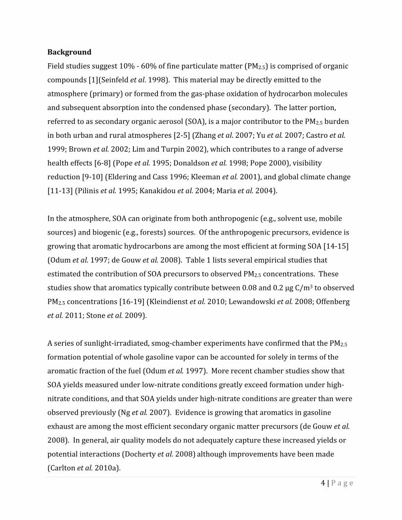
In the atmosphere, SOA can originate from both anthropogenic (e.g., solvent use, mobile

sources) and biogenic (e.g., forests) sources. Of the anthropogenic precursors, evidence is

growing that aromatic hydrocarbons are among the most efficient at forming SOA [14‐15]

(Odum et al. 1997; de Gouw et al. 2008). Table 1 lists several empirical studies that

estimated the contribution of SOA precursors to observed PM2.5 concentrations. These

studies show that aromatics typically contribute between 0.08 and 0.2 µg C/m3 to observed

PM2.5 concentrations [16‐19] (Kleindienst et al. 2010; Lewandowski et al. 2008; Offenberg

et al. 2011; Stone et al. 2009).

A series of sunlight‐irradiated, smog‐chamber experiments have confirmed that the PM2.5

formation potential of whole gasoline vapor can be accounted for solely in terms of the

aromatic fraction of the fuel (Odum et al. 1997). More recent chamber studies show that

SOA yields measured under low‐nitrate conditions greatly exceed formation under high‐

nitrate conditions, and that SOA yields under high‐nitrate conditions are greater than were

observed previously (Ng et al. 2007). Evidence is growing that aromatics in gasoline

exhaust are among the most efficient secondary organic matter precursors (de Gouw et al.

2008). In general, air quality models do not adequately capture these increased yields or

potential interactions (Docherty et al. 2008) although improvements have been made

(Carlton et al. 2010a).

5 | P a g e

In the United States, gasoline‐powered vehicles are the largest source of aromatic

hydrocarbons to the atmosphere (Simon et al. 2010). Most gasoline formulations consist of

approximately 20% aromatic hydrocarbons (EPA 2012), which are used in place of lead to

boost octane. Therefore, it has been suggested that removal of aromatics could reduce SOA

concentrations and yield a substantial public health benefit (Gray and Varcoe 2005). The

issue is complicated by the fact that any change to fuel composition will affect vehicular

emissions of various pollutants (e.g., hydrocarbons, carbon monoxide, oxides of nitrogen,

primary PM2.5) which, in turn, will react in the atmosphere to produce a different mix of

pollutants that may have adverse effects (e.g., Cook et al. 2011).

The purpose of this study is to estimate the public health impacts and social costs

associated with exposure to SOA from vehicular emissions of aromatic hydrocarbons. This

analysis provides a baseline case to explore the magnitude of the issue and against which to

evaluate the cost and impacts of potential substitutes for aromatics. The next section

describes the methods for the analysis, followed by results and a concluding discussion.

METHODS

Predicted secondary PM2.5 concentrations attributable to single‐ringed aromatic

hydrocarbons are estimated for a baseline year (2006) using the Community Multiscale Air

Quality model version 5.0 (CMAQv5.0). Given that regulatory models are known to

underestimate anthropogenic SOA formation (Volkamer et al. 2006; de Gouw et al. 2008;

Docherty et al. 2008), these results are compared to available data to estimate scaling

factors to adjust the model results. Adjusted PM2.5 concentrations are then used in the US

EPA Benefits and Mapping Program v4.0 (BenMAP) model to estimate morbidity health

and mortality outcomes associated with exposure to these concentrations across the lower

48 states (Abt Associates, Inc. 2011).

Exposure Concentrations

6 | P a g e

The CMAQ model is among the most widely used air quality models, with 3000+ registered

users in 100 different countries (www.cmaq‐model.org). Federal and State regulatory

agencies use CMAQ for policy analyses and for routine air quality forecasting (Foley et al.

2010). The model provides a means for quantitatively evaluating the impact of air quality

management policies prior to implementation. This analysis relied on CMAQv5.0 with the

Carbon Bond 2005 (CB05) chemical mechanism, which includes a fairly comprehensive list

of precursors that lead to SOA formation via both gas‐ and aqueous‐phase oxidation

processes, as well as particle‐phase reactions (Carlton et al. 2010a).

Air quality model simulations based on CMAQv5.0 are used to estimate the total

concentration of SOA from all single‐ring aromatic compounds (e.g., benzene, toluene,

xylenes) in 12km grid cells for many urban areas and 36km grid cells for the remaining

areas covering the lower 48 states for a baseline year (2006).

Potential Underestimates in Predictions of SOA Formation

Although CMAQv5.0 contains updated algorithms and processes for predicting SOA

formation, evidence suggests that the model may still underestimate secondary PM2.5

concentrations (Carlton et al. 2010a; Docherty et al. 2008; Zhang and Ying 2011),

particularly during the summer (Foley et al. 2010). Experiments conducted at Carnegie

Mellon University to study SOA formation from the photooxidation of toluene show

significantly larger SOA production than parameterizations employed in current air‐quality

models (Hildebrandt et al. 2010).

Using an organic tracer‐based source apportionment approach, independently conducted

research over the last five years provides increasing evidence that aromatic hydrocarbons

in gasoline contribute, depending on the specific region, approximately 0.1 to 0.45 μg/m3 of

PM (Lewandowski et al. 2008; Offenberg et al. 2011; Kleindienst et al. 2010; Stone et al.

2009).

Given our objective to estimate the public health impact of aromatic SOA, CMAQv5.0 model

results must be adjusted to reflect any biases in this PM2.5 component. Monthly‐averaged

7 | P a g e

model results are compared against empirical estimates of aromatic SOA concentrations

derived from ambient measurements of 2,3‐dihydroxy‐4‐oxopentanoic acid collected at

twelve locations across the U.S. (Lewandowski et al. 2008; Offenberg et al. 2011;

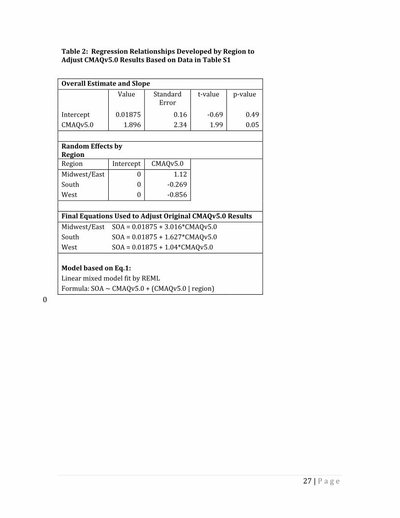
Kleindienst et al. 2010; Kleindienst et al. unpublished data). We develop region‐specific

regression relationships between predicted CMAQ and measured concentrations in µg of

carbon per m3 and use these to adjust the model results prior to estimating health effects.

We develop a mixed model with a random slope for each region, as there is some indication

that slopes should vary by region. For example, Hildebrandt et al. (2010) report elevated

SOA yields from toluene under high UV intensity, low‐NOx conditions, and lower

temperatures, relative to the parameters used typically in models. Therefore, the slope

might be low in CA where there is a lot of NOx and high in the Midwest and East where

ambient temperatures remain relatively low. The overall fixed effect and region‐specific

random effects models are developed using REML in R (http://www.r‐project.org/) based

on the following equation:

Formula: SOA ~ CMAQv5.0 + (CMAQv5.0 | region) (Eq. 1)

SOA Formation from Aromatic Hydrocarbons in Gasoline

SPECIATE, a US EPA database, provides a repository of volatile organic compound (VOC)

speciation profiles of air pollution sources. We use these source profiles in conjunction

with the 2005 National Emissions Inventory for VOCs to estimate the proportion of

aromatic SOA formation attributable to emissions from gasoline vehicles. We rank order

all sources of aromatic VOCs to quantify the contribution to total emissions specifically

from gasoline‐based sources.

Health and Mortality Impacts

The BenMAP model was used to estimate resulting health impacts associated with

exposures to the change in PM2.5 concentrations attributable to aromatic hydrocarbons

from gasoline vehicles predicted by the process described above. The BenMAP model is

widely used by regulatory agencies to quantify and monetize potential heath impacts

associated with changes in air quality, and contains concentration‐response functions for

8 | P a g e

various pollutants, including PM2.5, census data and population projections, and baseline

mortality and morbidity rates for the lower 48 United States. Concentration response

functions incorporated in BenMAP are based on published studies incorporating different

assumptions regarding potential thresholds and observed slopes between concentrations

and responses.

Four studies are included in this analysis (Krewski et al. 2009; Laden et al. 2006; Pope et al.

2002; Industrial Economics, Inc. 2006). Two major cohort studies are generally thought to

provide estimates regarded as most robust and applicable to the general population, with

the Harvard Six Cities Study publications reporting central estimates of an approximate

1.2‐1.6% increase in all‐cause mortality per μg/m3 increase in annual average PM2.5 (Laden

et al. 2006) and the American Cancer Society studies reporting estimates of approximately

0.4‐0.6% (Pope et al. 2002), with higher estimates when exposure characterization was

more spatially refined (Krewski et al. 2009). Within the expert elicitation study (Industrial

Economics, Inc. 2006) the median concentration‐response function across experts was

approximately 1%, midway between these cohort estimates, with a median 5th percentile

of 0.3% and a median 95th percentile of 2.0%. The EPA external Advisory Committee on

Clean Air Act Compliance Analysis recommended developing a distribution with the Pope

and Laden studies at the 25th and 75th percentiles, respectively, leading to a mean of the

new distribution close to the mean of the central estimates of both Pope and Laden. This

generally will be consistent with the distribution identified in the expert elicitation (US

EPA, SAB, HES, 2010). BenMAP applies these functions to the baseline mortality rate and

the number of people potentially exposed by census tract. BenMAP provides distributions

of premature mortality estimates based on the uncertainty in the concentration‐response

functions. That is, the 5th and 95th percentiles in the results are based on the distributions

for concentration‐response functions only.

Monetized Estimates of Premature Mortality

Monetized estimates of premature mortality are based on regulatory estimates of the value

of mortality risk as defined by the U.S. EPA

(http://yosemite.epa.gov/ee/epa/eed.nsf/pages/MortalityRiskValuation.html). This

9 | P a g e

estimate is based on research in which people are asked how much they would pay for

consumer products (such as water filters) that reduce risk or alternatively, that examine

how much more employers have to pay employees (adjusting for age, education,

experience, etc.) to compensate for taking an increased risk of accidental death. Hence this

estimate is not a price on a life, but a price of risk reduction. For convenience it is converted

into what was referred to as a value of a statistical life and is now referred to as the value of

mortality risk. The implication is if people are willing to pay $X for a reduction in risk of 1

in 10,000, than reducing risk in enough people to produce, on average, one fewer death

would be worth 10,000 X dollars. The U.S. EPA recommends a value of $7.4M in 2006 dollars

(USEPA 2010) based on over 30 labor market and contingent valuation studies.

RESULTS

CMAQv5.0 Modeling Results Compared to Measurements

Table S1 compiles measurement‐based estimates of aromatic SOA collected at twelve

locations between 2004 and 2010. Concentrations reach as high as 0.41 µgC/m3 during the

summer in Cincinnati, with a median value of 0.14 µgC/m3 across all 77 samples. In

contrast, the CMAQv5.0 model results from the corresponding 12km grid cells and

averaged over the appropriate month in 2006 show a maximum value of 0.13 and a median

of 0.052 µgC/m3 (see Table S1). This systematic bias in the model results warrants some

adjustment of the CMAQv5.0 output before it is used in the BenMAP calculations. The

mixed model obtained by regressing observations against the CMAQv5.0 results are shown

in Table 2. The slopes do differ by region, with the highest slopes observed in the East and

Midwest. Aggregated up to the national level, unadjusted CMAQ results predict a

nationwide average concentration of 0.0448 µg/m3, which increases to 0.17 following the

adjustment, a factor of approximately two, consistent with initial estimates ranging from

factors of two to five.

Predicted PM2.5 Concentrations from Aromatic Hydrocarbons in Gasoline

Source‐specific speciation of total VOC in the National Emissions Inventory reveals that the

U.S. emissions of aromatic hydrocarbons are 3.6 million tons per year, of which 69% are

10 | P a g e

from gasoline‐powered vehicles (Simon et al., 2010) as shown in Table 3. A source‐by‐

source breakdown of all aromatic hydrocarbon emissions is provided in Table S2. To

subtract the contribution of other emission sources (e.g., solvent usage, diesel exhaust)

from our calculations, the adjusted aromatic SOA concentrations from CMAQv5.0 are

multiplied by 0.69.

Spatial patterns of aromatic emissions are similar across sources. After gasoline, the next

highest source of aromatics is solvent usage, and Reff et al. (2009) show that the spatial

pattern of solvent usage is similar to gasoline, that is, occurs predominantly in urban areas.

In addition, most major refineries are also in close proximity to urban areas.

Adjusted CMAQv5.0 Results

Figure 1 shows the final nationwide distribution of annual average PM2.5 concentrations

attributable to aromatic hydrocarbons emitted from gasoline vehicles, after applying all the

adjustments to the CMAQv5.0 output described above. The nationwide average predicted

PM2.5 concentration based on the average predicted value for each state is approximately

0.124 μg/m3 (standard deviation = 0.059 μg/m3; minimum = 0.025 μg/m3, maximum =

0.227 μg/m3) and ranges from 0.013 to greater than 0.257 μg/m3 at the county level. On a

statewide basis, Table 4 shows the rank ordered concentrations by state, with Connecticut,

Rhode Island, Ohio, New York, New Jersey and Indiana predicted statewide concentrations

at 0.20 μg/m3 or higher.

BenMAP Modeling Results

Figure 2 presents a nationwide map of predicted premature mortalities attributable to

aromatic hydrocarbons in gasoline associated with the expert elicitation concentration‐

response function. Table 5 and Figure 3 provide a summary of predicted premature

mortality and monetized estimates of social cost based on all four different concentration‐

response functions. Predicted premature mortalities range from nearly 1,850 to more than

4,700 cases, depending on which concentration‐response function is used, which

correspond with approximately $13.6B to $34.9B in total social costs. The 5th and 95th

percentiles from each study are included in the parentheses, and represent the effect of

11 | P a g e

uncertainty in the concentration‐response functions only (e.g., there are many potential

sources of uncertainty, but only those associated with the concentration‐response

functions are captured in BenMap). Our recommended best estimate is approximately

3,800 premature mortalities based on the mean of the expert elicitation concentration‐

response function. Based on the central estimates from the Krewski and Laden studies,

respectively, results in a confidence interval of 1,850 to 4,700 for a central estimate.

The results in columns 3‐4 (a) in Table 5 are adjusted by 0.69 to account for the fraction of

aromatic emissions attributable to gasoline sources based on the National Emissions

Inventory. However, it is still possible that the fraction of aromatic emissions from gasoline

could be higher in urban areas (although, as noted previously, Reff et al. 2009 have shown

that spatial patterns of emissions from other sources of aromatics such as solvent usage are

similar to gasoline). To explore this assumption, we adjust only those counties designated

as rural counties (CDC 2012) by 0.69 and assume that 100% of emissions in urban areas

are derived from gasoline sources. The results are shown in the final two columns of Table

5 and in Figure 3. Predicted premature mortality increases to a little over 5,000, and based

on the concentration‐response function used, ranges from 2,400 to over 6,300.

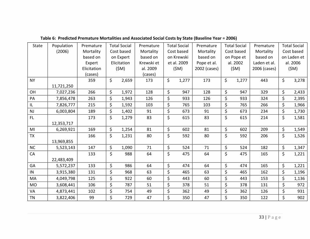
Table 6 provides predicted premature mortalities and associated social costs for each of

the four concentration‐response functions, adjusted by 0.69. Figure 4 provides the results

for each state, sorted from highest to lowest predicted impacts, using MetaDataViewer

available from the National Toxicology Program (Boyles et al. 2011) for the best estimate

represented by the expert elicitation slope (the remaining results are proportional based

on the results presented in Table 6; results not shown graphically). New York, with a

predicted average PM2.5 concentration of 0.21 μg/m3, shows the highest predicted impacts

based on the number of exposed individuals. Ohio and Pennsylvania follow, with

approximately 260 predicted premature mortalities each (based on the midpoint of the

combined expert elicitation concentration‐response function). The two states with the

highest population,, Texas and California, are ranked eighth and tenth, respectively, for

premature mortalities at approximately 160 and 130 expected cases, respectively.

12 | P a g e

DISCUSSION

The best estimate of potential impacts is based on the expert elicitation concentration‐

response function recently endorsed by a US EPA Science Advisory Board Panel together

with the regression‐based adjustment factors to the CMAQv5.0 predictions resulting in

3,800 predicted premature mortalities. This compares to a recent nationwide estimate of

approximately 130,000 overall premature mortalities (for 2005) associated with all PM2.5

exposures recently discussed by Fann et al. (2012) and based on the Krewski et al. (2009)

concentration‐response function. The results presented in Fann et al. (2012) were based

on CMAQv4.7 together with additional monitoring data to estimate premature mortalities

attributable to exposure to PM2.5 concentrations from all sources. The incremental

contribution from exposure to aromatic hydrocarbons in gasoline using the adjusted

results presented here and the Krewski concentration‐response function represents

approximately 1.4% of the total 130,000 estimated by Fann et al. (2012). While this may

seem a small fraction of total PM‐attributed mortality, these results are substantial as

compared to many public health measures, and with the Cross State Air Pollution Rule

implementation in the next five years, are likely to constitute a higher portion of PM‐

related deaths in the future. Under this rule, if SO2 emissions decrease by an expected 50%,

sulfate will become a smaller fraction of PM2.5; therefore, other sources will become more

important, particularly since SOA from aromatic hydrocarbon precursors are not expected

to decrease and could represent an increasingly larger fraction of exposures.

In addition to premature mortality, which dominates monetized estimates of total social

cost, exposures to SOA from aromatics in gasoline are associated with other health

outcomes, including exacerbation of asthma, upper respiratory symptoms, lost work days,

and hospital emergency room visits.

A recent study evaluated the public health impacts associated with exposure to direct

emissions of PM2.5 attributable to congested traffic conditions (Levy et al. 2010) and

estimated a total social cost of $31B (in 2007$), comparable to the central estimate of

$28.2B developed here. US EPA’s Heavy‐Duty Highway Diesel Final Rule estimates an

13 | P a g e

8,300 reduction in premature mortalities (US EPA 2006), a little more than twice the

number of premature mortalities from this analysis.

In some areas, particularly urban areas, anthropogenic precursors to SOA, and specifically

emissions from gasoline vehicles, are associated with contributions to PM2.5 ranging from

less than 5% to nearly 50% (Bahreini et al. 2012, Cabada et al. 2004; Wyche et al. 2009;

Docherty et al. 2008) . A recent study in Los Angeles (Bahreini et al. 2012) found that

gasoline emissions dominated SOA formation, accounting for nearly 90% of total aerosol

formation, and the ratio of SOA to primary organic aerosol was approximately a factor of

three. Across most areas in the U.S., SOA represents some 30%‐40% of organic carbon

concentrations (Yu et al. 2007; Pachon et al. 2010; Cabada et al. 2004; Zhang et al. 2009).

Many factors contribute to variability in SOA formation that are not well understood,

including spatial and chemical variability in emissions, the amount of time needed for PM

formation, and varying ambient conditions at different scales. CMAQ model performance of

SOA formation has improved substantially with each version of the model, but likely

doesn’t capture every process, given that SOA formation depends on varying atmospheric

physical and chemical conditions which are simulated at coarser scales in the CMAQ model

relative to the (unknown) scales at which they occur in the environment.

The error in aromatic SOA formation is estimated at approximately ±33% (Kleindienst et

al. 2007); therefore, measurements are somewhat better understood than the specific

processes and conditions leading to those observations. A strength of this analysis is the

combination of modeling corroborated by empirical studies to provide a baseline estimate

of predicted premature mortality associated with secondary particulate formation. We

provide an indication of the magnitude of the resulting public health burden that is more

likely to underestimate rather than overestimate potential impacts.The results show that

exposure to aromatic hydrocarbons in gasoline and resulting secondary organic aerosol

formation demonstrates a non‐trivial potential public health impact. As alternatives to

aromatics in gasoline are contemplated, it will be important to consider the potential public

health impacts associated with different transportation, fuel, and infrastructure design

14 | P a g e

options (see, for example, Cook et al. 2011, who developed a life‐cycle assessment

approach to evaluate the impacts of increased use of ethanol under several scenarios).

COMPETING INTERESTS

The authors declare no competing financial interests. Funding for KvS, JB, and JS was

provided by the Harvard Center for Risk Analysis. PVB participated as part of employment

with the US EPA.

AUTHORS’ CONTRIBUTIONS

KvS wrote the manuscript with oversight from JS, JB conducted the BenMAP modeling

using CMAQ results provided by PVB. All authors edited the final manuscript.

ACKNOWLEDGMENTS

Thanks go to Steven Melly for preparing Figures 1 and 2, and to Tad Kleindienst for

providing observational data from the California sites.

REFERENCES

Abt Associates, Inc. 2011. BenMAP: Environmental benefits and mapping analysis

program. Prepared for the US EPA Office of Air Quality Planning and Standards. Available

from (http://www.epa.gov/airquality/benmap/index.html); accessed January, 2012.

Bahreini R, Middlebrook AM, de Gouw JA, Warneke C, Trainer M, Brock CA, Start H, Brown

SS, Dube WP, Gilman JB, Hall K, Holloway JS, Kuster WC, Perring AE, Prevot ASH, Schwarz

JP, Spackman JR, Szidat S, Wagner NL, Weber RJ, Zotter P and Parrish DD. 2012. Gasoline

emissions dominate over diesel in formation of secondary organic aerosol mass.

Geophysical Research Letters 39:L06805, doi:10.1029/2011GL050718.

Bhave PV, Pouliot GA and Zheng M. 2007. Diagnostic model evaluation for carbonaceous

PM2.5 using organic markers measured in the Southeastern U.S. Environ Sci Technol

41:1577‐1583.

15 | P a g e

Boyles AL, Harris SF, Rooney AA and Thayer KA. 2011. Forest Plot Viewer: a new graphing

tool. Epidemiology 22(5):746‐747.

Brown SG, Herckes P, Ashbaugh L, Hannigan MP, Kreidenweis SM and Collett,

Jr, JL. 2002. Characterization of organic aerosol present in Big Bend National

Park, Texas during the Big Bend Regional Aerosol and Visibility Observational

(BRAVO) Study. Atmos Environ 36:5807‐5818.

Carlton AG, Bhave PV, Napelenok SL, Edney EO, Sarwar G, Pinder RW, Pouliot GA and

Houyoux M. 2010a. Model representation of secondary organic aerosol in CMAQv4.7.

Environ Sci Technol 44(22):8553–8560.

Carlton AG, Pinder RW, Bhave PV and Pouliot GA. 2010b. To what extent can biogenic SOA

be controlled? Environ Sci Technol 44(9):3376–3380.

Castro LM, Pio CA, Harrison RM and Smith DJT. 1999. Carbonaceous aerosol in urban and

rural European atmospheres: estimation of secondary organic carbon concentrations.

Atmos Environ 33:2771‐2781.

Centers for Disease Control (CDC). 2012. NCHS Urban–Rural Classification Scheme

for Counties. Vital and Health Statistics, Series 2, No. 154, January. U.S. Department of

Health and Human Services, National Center for Health Statistics. Available from

http://www.cdc.gov/nchs/data/series/sr_02/sr02_154.pdf, last accessed January 2013.

Chen J, Ying Q and Kleeman MJ. 2010. Source apportionment of wintertime secondary

organic aerosol during the California regional PM10/PM2.5 air quality study. Atmos

Environ 44:1331–1340.

Cook R, Phillips S, Houyous M, Dolwick P, Mason R, Yanca C, Zawacki M, Davidson K,

Michaels H, Harvey C, Somers J and Luecken D. 2011. Air quality impacts of increased use

16 | P a g e

of ethanol under the United States’ Energy Independence and Security Act. Atmos Env

45:7714‐7724.

Docherty KS, Stone EA, Ulbrich IM, DeCarlo PF, Snyder DC, Schauer JJ, Peltier RE, Weber RJ,

Murphy SM, Seinfeld JH, Grover BD, Eatough DJ and Jimenez JL. 2008. Apportionment of

primary and secondary organic aerosols in Southern California during the 2005 Study of

Organic Aerosols in Riverside (SOAR‐1). Environ Sci Technol 42:7655–7662.

Donaldson K, Li XY and MacNee W. 1998. Ultrafine (Nanometre) particle mediated lung

injury. Journal of Aerosol Science 29:553‐560.

Eldering A and Cass GR. 1996. Source‐oriented model for air pollutant effects on

visibility. J Geophys Res 101(D14)19:343‐19, 369.

Fann N, Lamson AD, Anenberg SC, Wesson K, Risley D and Hubbell BJ. 2012. Estimating

the national public health burden associated with exposure to ambient PM2.5 and ozone.

Risk Anal 32(1):81‐95.

Foley KM, Roselle SJ, Appel KW, Bhave PV, Pleim JE, Otte TL, Mathur R, Sarwar G, Young JO,

Gilliam RC, Nolte CG, Kelly JT, Gilliland AB and Bash JO. 2010. Incremental testing of the

Community Multiscale Air Quality (CMAQ) modeling system version 4.7. Geosci Model Dev

3:205–226, www.geosci‐model‐dev.net/3/205/2010/.

de Gouw JA, Brock CA, Atlas EL, BAtes TS, Fehsenfeld FC, Goldan PD, Holloway JS, Kuster

WC, Lerner BM, Matthew BM, Middlebrook AM, Onasch TB, Peltier RE, Quinn PK, Senff CJ,

Stohl A, Sullivan AP, Trainer M, Warneke C, Weber RJ and Williams EJ. 2008. Sources of

particulate matter in the northeastern United States in summer: 1. Direct emissions and

secondary formation of organic matter in urban plumes. J Geophys Res 113:D08301,

doi:10.1029/2007JD009243.

17 | P a g e

de Gouw JA, Middlebrook AM, Warneke C, Goldan PD, Kuster WC, Roberts JM, Fehsenfeld

FC, Worsnop DR, Canagaratna MR, Pszenny AAP, Keene WC, Marchewka M, Bertman SB and

Bates TS. 2005. Budget of organic carbon in a polluted atmosphere: Results from the New

England Air Quality Study in 2002. J Geophys Res 110:D16305,

doi:10.1029/2004JD005623.

Gray CB and Varcoe AR. 2005. Octane, clean air, and renewable fuels: A modest

step toward energy independence, Texas Review of Law & Politics 10:9–62.

Harley RA, Hannigan MP and Cass GR. 1992. Respeciation of organic gas emissions and the

detection of excess unburned gasoline in the atmosphere. Environ Sci Technol 26:2395–

2408.

Hildebrandt L, Donahue NM and Pandis SN. 2009. High formation of secondary organic

aerosol from the photo‐oxidation of toluene. Atmos Chem Phys 9:2973–2986, www.atmos‐

chem‐phys.net/9/2973/2009/.

Hoyle CR, Boy M, Donahue NM, Fry JL, Glasius M, Guenther A, Hallar AG, Huff Hartz K,

Petters MD, Pet T, Rosenoern T and Sullivan AP. 2011. A review of the anthropogenic

influence on biogenic secondary organic aerosol. Atmos Chem Phys 11:321–343,

www.atmos‐chem‐phys.net/11/321/2011/doi:10.5194/acp‐11‐321‐2011.

Hoyle CR, Boy M, Donahue NM, Fry JL, Glasius M, Guenther A, Hallar AG, Huff Hartz K,

Petters MD, Pet T, Rosenoern T and Sullivan AP. 2010. Anthropogenic influence on

biogenic secondary organic aerosol. Atmos Chem Phys Discuss 10:19515–19566,

www.atmos‐chem‐phys‐discuss.net/10/19515/2010/ doi:10.5194/acpd‐10‐19515‐2010.

Industrial Economics, Inc. 2006. Expanded expert judgment assessment of the

concentration‐response relationship between PM2.5 exposure and mortality. Cambridge,

MA: Prepared for Office of Air Quality Planning and Standards, US Environmental

Protection Agency.

18 | P a g e

Kanakidou M, Seinfeld JH, Pandis SN, Barnes I, Dentener FJ, Facchini MC, van Dingenen R,

Ervens B, Nenes A, Nielsen CJ, Swietlicki E, Putaud JP, Balkanski Y, Fuzzi S, Horth J,

Moortgat GK, Winterhalter R, Myhr CEL, Tsigaridis K, Vignati E, Stephanou EG and Wilson J.

2004. Organic aerosol and global climate modelling: a review. Atmospheric Chemistry and

Physics Discussions (SMOCC Special Issue) 4:5855‐6024.

Ke L, Ding X, Tanner RL, Schauer JJ and Zheng M. 2007. Source contributions to

carbonaceous aerosols in the Tennessee Valley Region. Atmospheric Environment

41(39):8898–8923.

Kleeman MJ, Riddle SG, Robert MA, Jakober CA, Fine PM, Hays MD, Schauer JJ, Hannigan MP.

2009. Source apportionment of fine (PM1.8) and ultrafine (PM0.1) airborne particulate

matter during a severe winter pollution episode. Environmental Science & Technology 32,

272–279.

Kleeman MJ, Ying Q, Lu J, Mysliwiec MJ, Griffin RJ, Chen J, Clegg S. 2007. Source

apportionment of secondary organic aerosol during a severe photochemical

smog episode. Atmos Environ 41:576–591.

Kleeman MJ, Eldering A, Hall JR and Cass GR. 2001. Effect of emissions control

programs on visibility in southern California. Environ Sci Technol 35:4668 – 4674.

Kleindienst TE, Lewandowski M, Offenberg JH, Edney EO, Jaoui M, Zheng M, Ding X and

Edgerton ES. 2010. Contribution of primary and secondary sources to organic aerosol at

SEARCH network sites. J Air Waste Manage Assoc 60:1388–1399.

Kleindienst TE, Jaoui M, Lewandowski M, Offenberg JH, Lewis CW, Bhave PV and Edney EO.

2007. Estimates of the contributions of biogenic and anthropogenic hydrocarbons to

secondary organic aerosol at a southeastern US location. Atmos Environ 41:8288‐8300.

doi:10.1016/j.atmosenv.2007.06.045.

19 | P a g e

Kleindienst TE, Corse EW, Li W, McIver CD, Conver TS, Edney EO, Driscoll DJ, Speer RE,

Weathers WS and Tejada SB. 2002. Secondary organic aerosol formation from the

irradiation of simulated automobile exhaust. J Air Waste Manage Assoc 52:259–272.

Koo BY, Ansari AS and Pandis SN. 2003. Integrated approaches to modeling the organic and

inorganic atmospheric aerosol components. Atmos Environ 37(34):4757–4768.

Krewski D, Jerrett M, Burnett RT, Ma R, Hughes E, Shi Y, Turner MC, Pope CA III, Thurston G,

Calle EE, Thun MJ, Beckerman B, DeLuca P, Finkelstein N, Ito K, Moore DK, Newbold KB,

Ramsay T, Ross Z, Shin H, Tempalski B. 2009. Extended follow‐up and spatial analysis of the

American Cancer Society study linking particulate air pollution and mortality. Res Rep

Health Eff Inst 140:5‐114.

Laden F, Schwartz J, Speizer FE and Dockery DW. 2006. Reduction in fine particulate air

pollution and mortality: Extended follow‐up of the Harvard Six Cities Study. Am J Respir Crit

Care Med 173(6):667‐72.

Lane TE, Donahue NM and Pandis SN. 2008. Simulating secondary organic aerosol

formation using the volatility basis‐set approach in a chemical transport model. Atmos

Environ 42:7439–7451, doi:10.1016/j.atmosenv.2008.06.026.

Levy J, Buonocore J and K von Stackelberg. 2010. Evaluation of the public health impacts of

traffic congestion. Environmental Health 9:65‐doi:10.1186/1476‐069X‐9‐65.

Lewandowski M, Jaoui M, Offenberg JH, Kleindienst TE, Edney EO, Sheesley R and Schauer

JJ. 2008. Primary and secondary contributions to ambient PM in the midwestern United

States. Environ Sci Technol 42(9):3303‐3309.

20 | P a g e

Lim H‐J and Turpin BJ. 2002. Origins of primary and secondary organic aerosols in Atlanta:

results of time‐resolved measurements during the Atlanta supersite experiment. Environ

Sci Technol 36:4489‐4496.

Maria SF, Russell LM, Gilles MK and Myneni SCB. 2004. Organic aerosol

growth mechanisms and their climate‐forcing implications. Science 306:1921‐

1924.

Ng NL, Kroll JH, Chan AWH, Chhabra PS, Flagan RC, Seinfeld JH. 2007. Secondary organic

aerosol formation from m‐xylene, toluene, and benzene. Atmos Chem Phys Discuss 7:3909–

3922.

Odum JR, Jungkamp TPW, Griffin RJ, Flagan RC and Seinfeld JH. 1997. The atmospheric

aerosol‐forming potential of whole gasoline vapor. Science 276:96‐99.

Offenberg JH, Lewandowski M, Jaoui M and Kleindienst TE. 2011. Contributions of

biogenic and anthropogenic hydrocarbons to secondary organic aerosol during 2006 in

Research Triangle Park, NC. Aerosol Air Qual Res 11:99–108.

Pachon JE, Balachandran S, Hu Y, Weber RJ, Mulholland JA and Russell AG. 2010.

Comparison of SOC estimates and uncertainties from aerosol chemical composition and gas

phase data in Atlanta. Atmos Env 44(32):3907‐3914.

Pandis SN, Harley RA, Cass GR and Seinfeld JH. 1992. Secondary organic aerosol formation

and transport. Atmos Environ 26A(13):2269‐2282.

Pilinis C, Pandis S and Seinfeld JH. 1995. Sensitivity of direct climate forcing by

atmospheric aerosols to aerosol size and composition. J Geophys Res 100(18):739‐754.

21 | P a g e

Pope CA 3rd, Burnett RT, Thun MJ, Calle EE, Krewski D, Ito K and Thurston GD. 2002. Lung

cancer, cardiopulmonary mortality, and long‐term exposure to fine particulate air

pollution. JAMA 287(9):1132‐41.

Schauer JJ, et al. 1996. Source apportionment of airborne particulate matter using organic

compounds as tracers. Atmos Environ 30:3837–3855.

Seinfeld JH and Pandis SN. Atmospheric Chemistry and Physics: From Air

Pollution to Climate Change, John Wiley & Sons, New York, 1998.

Simon H, Beck L, Bhave PV, Divita F, Hsu Y, Luecken D, Mobly JD, Pouliot GA, Reff A, Sarwar

G and Strum M. 2010. The development and uses of EPA’s SPECIATE database.

Atmospheric Pollution Research 1:196‐206.

Stone EA, Zhou J, Snyder DC, Rutter, AP, Mieritz M and Schauer JJ. 2009. A comparison of

summertime secondary organic aerosol source contributions at contrasting urban

locations. Environ Sci Technol 43(10):3448‐3454.

Tanner RL, Parkhurst WJ, Valente ML and Philips WD. 2004. Regional composition of PM2.5

aerosols measured at urban, rural and "background" sites in the Tennessee valley. Atmos

Environ 38:3143‐3153.

United States Environmental Protection Agency (USEPA). 2012. Reformulated gasoline

parameters by reporting year. Available from:

http://www.epa.gov/otaq/regs/fuels/rfg/properf/rfg‐params97‐02.htm. Accessed March

31, 2012.

United States Environmental Protection Agency (USEPA). 2010. Guidelines for preparing

economic analyses. National Center for Environmental Economics. Available from

http://yosemite.epa.gov/ee/epa/eed.nsf/pages/Guidelines.html, accessed January, 2012.

22 | P a g e

United States Environmental Protection Agency (USEPA). 2006. Program update.

Introduction of cleaner‐burning diesel fuel enables advanced pollution control for cars,

trucks and buses. Office of Transportation and Air Quality. EPA420‐F‐06‐064, October

2006. Available from http://www.epa.gov/otaq/highway‐diesel/index.htm, accessed July

2012.

United States Environmental Protection Agency (USEPA), Advisory Council of the Clean Air

Act, Health Effects Subcommittee (HES) of the Council. 2010. Review of EPA’s Draft Health

Benefits of the Second Section 812 Prospective Study of the Clean Air Act.” (EPA‐COUNCIL‐

10‐001), available at http://www.epa.gov/advisorycouncilcaa, accessed July 2012.

Volkamer R, Jimenez JL, San Martini F, Dzepina K, Zhang Q, Salcedo D, Molina LT, Worsnop

DR and Molina MJ. 2006. Secondary organic aerosol formation from anthropogenic air

pollution: Rapid and higher than expected. Geophys Res Letters 33:L17811,

doi:10.1029/2006GL026899.

Weber RJ, Sullivan AP, Peltier RE, Russell A, Zheng BM de Gouw J, Warneke C, Brock C,

Holloway JS, Atlas EL and Edgerton E. 2007. A study of secondary organic aerosol

formation in the anthropogenic‐influenced southeastern United States. J Geophys Res

112:D13302, doi:10.1029/2007JD008408.

Williams BJ, Goldstein AH, Kreisberg NM, Hering SV, Worsnop DR, Ulbrich IM, Docherty KS

and Jiminez JL. 2010. Major components of atmospheric organic aerosol in southern

California as determined by hourly measurements of source marker compounds. Atmos

Chem Phys 9 10, 11577–11603, www.atmos‐chem‐phys.net/10/11577/2010/,

doi:10.5194/acp‐10‐11577‐2010.

Wyche KP, Monks PS, Ellis AM, Cordell RL, Parker AE, Whyte C, Metzger A, Dommen J,

Duplissy J, Prevot ASH, Baltensperger U, Rickard AR and Wulfert F. 2009. Gas phase

precursors to anthropogenic secondary organic aerosol: detailed observations of 1,3,5‐

23 | P a g e

trimethylbenzene photooxidation. Atmos Chem Phys 9:635–665, www.atmos‐chem‐

phys.net/9/635/2009/.

Yin JX, Harrison RM, Chen Q, Rutter A and Schauer JJ. 2010. Source apportionment of fine

particles at urban background and rural sites in the UK atmosphere. Atmos Environ

30(44):841–851.

Yu S, Bhave PV, Dennis RL and Mathur R. 2007. Seasonal and regional variations of

primary and secondary organic aerosols over the continental United States: Semi‐empirical

estimates and model evaluation. Environ Sci Technol 41(13):4690‐4697.

Zhang H and Ying Q. 2011. Secondary organic aerosol formation and source

apportionment in Southeast Texas. Atmos Environ 45(19):3217‐3227.

Zhang Q, Jiminez JL, Canagaratna MR, Ulbrich IM, Ng NL, Worsnop DR and Sun Y. 2011.

Understanding atmospheric organic aerosols via factor analysis of aerosol mass

spectrometry: a review. Anal Bioanal Chem 401:3045–3067, DOI 10.1007/s00216‐011‐

5355‐y

Zhang Q, Jiminez JL, Canagaratna MR, Allan JD, Coe H, Ulbrich I, Alfarra MR, Takami A,

Middlebrook AM, Sun YL, Dzepina K, Dun;lea E, Docherty K, DeCarlo PF, Salcedo D, Onasch

T, Jayne JT, Miyoshi T, Shimono A, Hatakeyama S, Takegawa N, Kondo Y, Schneider J,

Drewnick F, Borrmann S, Weimer S, Demerjian K, Williams P, Bower K, Bahreini R, Cottrell

L, Griffin RJ, Rautiainen J, Sun JY, Zhang YM and Worsnop DR. 2007. Ubiquity and

dominance of oxygenated species in organic aerosols in anthropogenically‐influenced

Northern Hemisphere midlatitudes. Geophysical Research Letters 34:L13801,

doi:10.1029/2007GL029979.

Zhang Y, Sheesley R, Schauer JJ, Lewandowski M, Jaoui M, Offenberg JH, Kleindienst TE and

Edney EO. 2009. Source apportionment of primary and secondary organic aerosols using

positive matrix factorization (PMF) of molecular markers. Atmos Env 43:5567‐5574.

24 | P a g e

25 | P a g e

Figure 1: Annual Average PM2.5 Concentrations Attributed to Aromatic Emissions from

Gasoline Vehicles

Figure 2: Estimated Cases of Premature Mortality Based on the Consensus Expert

Elicitation Concentration‐Response Function

Figure 3: Incidence and Total Social Cost Associated with Exposure to Aromatic SOA from

Gasoline Emissions

Figure 4: Total Social Costs by State Based on Expert Elicitation Concentration‐Response

Function

26 | P a g e

Table 1: Studies Evaluating the Contribution of Aromatic Hydrocarbons to SOA

Reference Description Source Apportionment Concentrations (µg/m3)

Kleindienst et al. 2010 Contribution of primary and secondary sources of OC to PM2.5 in Southeastern Aerosol Research and Characterization (SEARCH) network samples

Toluene used as a chemical tracer (2,3‐ hydroxy‐4‐oxopentanoic acid)

0.10 to 0.45 across 4 sampling locations

Lewandowski et al. 2008 Contribution of primary and secondary sources of OC to PM2.5 in five midwestern United States cities throughout 2004: East St. Louis, IL Detroit, MI Cincinnati, OH Bondville, IL and Northbrook, IL


Bondville: 0.09 ‐ 0.25; Northbrook: 0.06 ‐ 0.21; Cincinnati: 0.02 ‐ 0.29; Detroit: 0.07 ‐ 0.33; East St. Louis: 0.06 ‐ 0.26

Offenberg et al. 2011 Contribution of primary and secondary sources of OC to PM2.5 in 2006 in Research Triangle Park, NC over the course of a year


average = 0.1, stdev = 0.09, min = 0.02, max = 0.36, n=33

Williams et al. 2010 Positive matrix factorization to determine primary and secondary components of organic aerosol

SOA from motor vehicles contribute 11% of total organic aerosols

concentrations not provided

Stone et al. 2009 Contribution of primary and secondary sources of OC to PM2.5 in July‐August 2007 in Cleveland, OH, Detroit, MI and LA, CA


0.05 ‐ 1.1 in the midwest; 0.95 ‐ 1.61 in CA

27 | P a g e

Table 2: Regression Relationships Developed by Region to Adjust CMAQv5.0 Results Based on Data in Table S1

Overall Estimate and Slope

Value Standard Error

t‐value p‐value

Intercept 0.01875 0.16 ‐0.69 0.49CMAQv5.0 1.896 2.34 1.99 0.05

Random Effects by Region

Region Intercept CMAQv5.0

Midwest/East 0 1.12South 0 ‐0.269West 0 ‐0.856

Final Equations Used to Adjust Original CMAQv5.0 Results

Midwest/East SOA = 0.01875 + 3.016*CMAQv5.0South SOA = 0.01875 + 1.627*CMAQv5.0West SOA = 0.01875 + 1.04*CMAQv5.0

Model based on Eq.1: Linear mixed model fit by REML Formula: SOA ~ CMAQv5.0 + (CMAQv5.0 | region)

0

28 | P a g e

Table 3: National Emissions Inventory of Aromatic Hydrocarbons

Source Aromatic VOC (ton/yr)

% of Total

Gasoline 2,491,313

69%

Solvent Usage 518,334 14%Diesel 25,436 1%Other 573,679 16%Total

3,608,762 100%

Note: This information was obtained by combining VOC emissions from the National Emissions Inventory with speciation profiles from the SPECIATE database. See Table S2. 1

2

29 | P a g e

Table 4: State‐wide Annual Average Estimates of PM2.5

Attributed to Aromatic SOA from Gasoline Emissions

State Predicted PM2.5

Concentration (µg/m3)

CT 0.23 RI 0.23 OH 0.21 NY 0.21 NJ 0.20 IN 0.20 MA 0.19 NH 0.18 IL 0.17 PA 0.17 MO 0.17 MI 0.16 SC 0.16 NC 0.16 GA 0.16 VT 0.15 IA 0.15 WI 0.15 ME 0.14 KY 0.14 DE 0.14 TN 0.14 AL 0.14 WV 0.13 VA 0.13 MS 0.13 KS 0.12 DC 0.12 MD 0.12 AR 0.11 MN 0.11

30 | P a g e

NE 0.11 OK 0.09 LA 0.09 SD 0.09 TX 0.08 ND 0.08 FL 0.08 NV 0.05 AZ 0.05 CA 0.04 ID 0.04 MT 0.03 UT 0.03 WY 0.03 OR 0.03 WA 0.03 NM 0.03 CO 0.03 3

4

31 | P a g e

5

32 | P a g e

Table 5: Premature Mortality and Total Social Cost for Health Impacts Associated with Exposure to SOA from Aromatic Hydrocarbons in Gasoline in the Lower 48 States

Reference Beta Premature Mortality (cases)

Value of Mortality Reduction ($M)

Laden et al. 2006 0.015 4714 (2533, 6897) $34.9B ($18.7B, $51.0B) Pope et al. 2002 0.006 1833 (717, 2951) $13.6B ($5.3B, $21.8B) Krewski et al. 2009 0.006 1833 (1335, 2332) $13.6B ($9.9B, $17.2B) Expert Elicitation 0.011 3816 (886, 6814) $28.2B ($6.6B, $50.4B) Notes: Value of mortality reduction = $7.4M per case in 2006$ 6

7

33 | P a g e

Table 6: Predicted Premature Mortalities and Associated Social Costs by State (Baseline Year = 2006)

State Population (2006)

Premature Mortality based on Expert

Elicitation (cases)

Total Social Cost based on Expert Elicitation

($M)

Premature Mortality based on Krewski et al. 2009 (cases)

Total Social Cost based on Krewski et al. 2009

($M)

Premature Mortality based on Pope et al. 2002 (cases)

Total Social Cost based on Pope et al. 2002 ($M)

Premature Mortality based on Laden et al. 2006 (cases)

Total Social Cost based on Laden et al. 2006 ($M)

NY 11,721,250

359 $ 2,659 173 $ 1,277 173 $ 1,277 443 $ 3,278

OH 7,027,236 266 $ 1,972 128 $ 947 128 $ 947 329 $ 2,433 PA 7,856,478 263 $ 1,943 126 $ 933 126 $ 933 324 $ 2,395 IL 7,826,777 215 $ 1,592 103 $ 765 103 $ 765 266 $ 1,966 NJ 6,003,804 189 $ 1,402 91 $ 673 91 $ 673 234 $ 1,730 FL

12,353,717 173 $ 1,279 83 $ 615 83 $ 615 214 $ 1,581

MI 6,269,921 169 $ 1,254 81 $ 602 81 $ 602 209 $ 1,549 TX

13,969,855 166 $ 1,231 80 $ 592 80 $ 592 206 $ 1,526

NC 5,523,143 147 $ 1,090 71 $ 524 71 $ 524 182 $ 1,347 CA

22,483,409 133 $ 988 64 $ 475 64 $ 475 165 $ 1,221

GA 5,572,237 133 $ 986 64 $ 474 64 $ 474 165 $ 1,221 IN 3,915,380 131 $ 968 63 $ 465 63 $ 465 162 $ 1,196 MA 4,049,798 125 $ 922 60 $ 443 60 $ 443 153 $ 1,136 MO 3,608,441 106 $ 787 51 $ 378 51 $ 378 131 $ 972 VA 4,873,441 102 $ 754 49 $ 362 49 $ 362 126 $ 931 TN 3,822,406 99 $ 729 47 $ 350 47 $ 350 122 $ 902

34 | P a g e

WI 3,619,422 84 $ 624 40 $ 300 40 $ 300 104 $ 769 CT 2,253,322 83 $ 617 40 $ 296 40 $ 296 103 $ 761 SC 2,772,416 82 $ 605 39 $ 291 39 $ 291 101 $ 749 AL 2,927,474 81 $ 599 39 $ 288 39 $ 288 100 $ 742 KY 2,675,868 69 $ 507 33 $ 244 33 $ 244 85 $ 628 MD 3,715,953 67 $ 493 32 $ 237 32 $ 237 82 $ 610 MN 3,314,038 54 $ 397 26 $ 191 26 $ 191 66 $ 490 IA 1,906,272 48 $ 353 23 $ 170 23 $ 170 59 $ 435 MS 1,846,049 45 $ 335 22 $ 161 22 $ 161 56 $ 416 LA 2,630,768 43 $ 315 20 $ 151 20 $ 151 53 $ 391 AR 1,803,802 40 $ 296 19 $ 142 19 $ 142 49 $ 366 OK 2,233,442 38 $ 283 18 $ 136 18 $ 136 47 $ 350 KS 1,680,031 35 $ 257 17 $ 123 17 $ 123 43 $ 317 WV 1,187,545 33 $ 242 16 $ 116 16 $ 116 40 $ 298 AZ 3,911,781 29 $ 217 14 $ 104 14 $ 104 36 $ 269 NH 952,282 26 $ 190 12 $ 91 12 $ 91 32 $ 234 RI 653,356 25 $ 187 12 $ 90 12 $ 90 31 $ 230 ME 904,612 23 $ 169 11 $ 81 11 $ 81 28 $ 208 NE 1,058,917 19 $ 140 9 $ 67 9 $ 67 23 $ 172 WA 4,138,920 18 $ 135 9 $ 65 9 $ 65 22 $ 166 NV 1,603,777 14 $ 101 7 $ 49 7 $ 49 17 $ 125 DE 522,705 13 $ 95 6 $ 45 6 $ 45 16 $ 117 OR 2,383,414 12 $ 90 6 $ 43 6 $ 43 15 $ 111 VT 436,489 10 $ 77 5 $ 37 5 $ 37 13 $ 95 CO 2,974,597 9 $ 70 5 $ 34 5 $ 34 12 $ 87 SD 473,989 7 $ 53 3 $ 25 3 $ 25 9 $ 65

35 | P a g e

NM 1,300,700 6 $ 47 3 $ 22 3 $ 22 8 $ 58 UT 1,399,252 6 $ 45 3 $ 22 3 $ 22 8 $ 56 ND 413,558 5 $ 41 3 $ 19 3 $ 19 7 $ 50 ID 907,667 5 $ 38 2 $ 18 2 $ 18 6 $ 47 MT 639,955 4 $ 29 2 $ 14 2 $ 14 5 $ 35 DC 217,088 4 $ 28 2 $ 14 2 $ 14 5 $ 35 WY 347,896 2 $ 13 1 $ 6 1 $ 6 2 $ 16 8

9

36 | P a g e

10

37 | P a g e

Table S1: Comparison of Observed SOA Measurements and Unadjusted CMAQv5.0 11

Predictions 12

13

Table S2: US EPA's SPECIATE Database Used to Determine the Fraction of 14

Anthropogenic SOA from Aromatic Hydrocarbons in Gasoline 15

Health Impacts of Secondary Hydrocarbons in Gasoline

Documents

Transcript of Health Impacts of Secondary Hydrocarbons in Gasoline