Health Disparities and the Socioeconomic Gradientin Elderly Life-Cycle Consumption∗

Ray Miller† Neha Bairoliya‡ David Canning§

June 27, 2018

Abstract

We quantify the importance of health disparities in explaining consumptiondifferences at older ages by estimating a panel VARmodel of elderly consumption,health, and mortality using data from the Health and Retirement Study. We usethe estimated model and initial joint distribution of health and consumptionto simulate elderly life-cycle paths and construct a measure of the net presentvalue of expected remaining lifetime consumption at age sixty (NPVC). We firstdocument a steep education gradient in elderly lifetime consumption. We thendecompose the gradient in NPVC to quantify the effect of 1) differences in thehealth distribution at age sixty and 2) differential health and mortality transitionsafter age sixty. Our decomposition results suggest that roughly 11-12% of theeducation gradient in NPVC at age sixty could be closed by eliminating elderlyhealth differences.

JEL classifications: D12, D30, D63, I14Keywords: consumption inequality, health, aging, education gradient, life-cycle

∗Research reported in this publication was supported by the National Institute on Aging of theNational Institutes of Health under Award Number P30AG024409 and by the National Institutes ofHealth (NIH, Grant No.: 5R01AG048037-02). The content is solely the responsibility of the authorsand does not necessarily represent the official views of the National Institutes of Health. The HRS(Health and Retirement Study) is sponsored by the National Institute on Aging (grant number NIAU01AG009740) and is conducted by the University of Michigan.†Corresponding author. Harvard Center for Population and Development Studies, Cambridge,

MA, 02138. Email: hrmiller@hsph.harvard.edu‡Harvard Center for Population and Development Studies§Harvard T.H. Chan School of Public Health

1

1 IntroductionThe turn of the century has witnessed not only a rise in economic inequality but alsogrowing disparities in health and mortality.1 While the correlations between healthand economic circumstances have been widely studied, it is less clear to what extentvariations in the former may translate into the latter. In this study, we examine thedynamic relationship between health and consumption over the elderly life course. Indoing so, we shed light on the potential impact of policies that promote health equityon broader economic inequality among the elderly.

Adverse health shocks may influence individual or household consumption througha variety of mechanisms. These effects could be contemporaneous, for example throughincreased expenditures on medical care, reduced earnings, or decreased consumption ofgoods and services that are complements to good health. Or there could be dynamiceffects that persist over time, for example through forced early retirement or perhapseven expedited death. In any case, these channels suggest that variations in health mayexplain, at least partly, the disparate consumption patterns observed across socioeco-nomic groups in the U.S. This relationship could be especially important at older ageswhere mortality rates are high and most of the variance in health across individuals isconcentrated (Deaton and Paxson, 1998).

Understanding the extent to which health differences influence consumption inequa-lity is a challenging task. Health is a multidimensional concept with many proposedsubjective and objective measures (e.g. self-rated health, physical limitations, incidenceof morbidities, etc). Different types of health events can impact consumption, bothcurrent and future, with varying intensities—a cardiac event may have a stronger andmore persistent effect on consumption than hypertension. There is also the possibilityof dynamic spillovers across health conditions—hypertension is a risk factor knownto increase the likelihood of other adverse health outcomes including death (Ettehadet al., 2016). Finally, individuals with similar annual consumption but substantiallydifferent lifespans will have very different total lifetime consumption. Moreover, thelife-cycle hypothesis suggests an unexpected health shock could potentially increasecontemporaneous consumption if there is an associated decline in life expectancy. Inthese cases, cross-sectional associations between consumption and health would onlybe presenting a part of the bigger story.

In light of these potentially dynamic and multi-faceted influences, we take a life-cycle approach to better quantify the total contribution of health disparities to diffe-rential consumption patterns over elderly life in the U.S. Using a similar frameworkas Miller and Bairoliya (2018), we estimate a panel vector autoregressive (VAR) mo-del to approximate the joint evolution of consumption, mortality, and a multivariatemeasure of health over the elderly life-cycle. We use longitudinal data from the He-alth and Retirement Study (HRS) supplemented with the Consumption and Activities

1Refer to Heathcote et al. (2010); Cutler and Katz (1992); Katz et al. (1999); Attanasio et al. (2014)for rising economic inequality and Chetty et al. (2016); National Academies of Sciences, Engineering,and Medicine (2015); Meara et al. (2008); Case and Deaton (2017) for health and mortality.

2

Mail Survey (CAMS). Together, these provide a long and rich panel (1992-2014) forstudying the joint distribution of health and consumption for the elderly. We use theestimated system to simulate and analyze potential outcome paths for a sub-sample ofHRS respondents. Using the simulated paths for consumption and mortality, we con-struct a measure of the net present value of expected remaining lifetime consumption(NPVC) at age sixty. This measure, which can also be viewed as an age sixty wealthequivalent, provides a parsimonious setup for studying both the contemporaneous aswell as dynamic effects of health in driving consumption differences.

In order to examine the influence of health disparities on consumption inequality,we study differences across educational attainment levels. We choose to focus on thissocioeconomic dimension as substantial education gradients have been well documen-ted in health and mortality (Conti et al., 2010; Pijoan-Mas and Ríos-Rull, 2014) as wellas income (Houthakker, 1959; Morgan and David, 1963; Griliches and Mason, 1972).It is well known that income differences across education groups primarily stem fromdifferential returns to education. While some of these income differences may furthertranslate into health differences due to differential access to medical goods and services,studies show that differences in health outcomes are also due to differences in healthbehaviors (Cutler and Lleras-Muney, 2010), knowledge capital (Kenkel, 1991) and ad-herence to medication (Goldman and Smith, 2002). We do not focus on the reasonsunderlying the observed education gradients in health and consumption in this analy-sis, rather we ask how much of the education-consumption gradient can be attributedto health disparities across education groups. We further decompose how much of thegradient can be explained by differences in initial (age sixty) health distribution versusthe differential evolution of health and mortality after age sixty across these groups.

Our main results are summarized as follows: we first document a substantial edu-cation gradient in cross-sectional consumption at age sixty—average consumption ofcollege graduates is 2.5 times higher than high school dropouts. This ratio rises to 3.0when examining NPVC—our estimate of elderly lifetime consumption. This rise is dueto a positive correlation between consumption, health, and longevity. For example, weestimate that the average life expectancy of college graduates at age sixty is 5.4 yearslonger than high school dropouts. So not only are the college educated enjoying moreaverage consumption in the cross-section, they enjoy the consumption for a longer andhealthier period of time.

Our second set of results quantify the influence of health disparities on the education-consumption gradient. First, we find that conditional on health, differential survivalrates across education groups actually explain very little of the gap in NPVC. Thereason is that we do not find a strong education gradient in mortality rates after con-trolling for health. This finding is consistent with those reported by Pijoan-Mas andRíos-Rull (2014). The authors also find that education, wealth, and income have verylittle impact on survival conditional on health. We do find, however, that the differen-tial evolution of health can explain an important share of the estimated consumptiondisparities. For instance, eliminating differential elderly health transitions after sixty(mortality, morbidities, and subjective health) across education groups can close an

3

estimated 5.7% of the educational gradient in NPVC between college graduates andhigh school dropouts at age sixty. However, this is a lower bound of the overall effectas part of the gradient is driven by initial age sixty health conditions. When we givethe initial health distribution of the college graduates to those with less than a highschool education, the consumption gradient closes by 5.1%. Altogether, we estimatethat the distribution of health at age sixty and subsequent health transitions combineto explain approximately 11% of the gap in NPVC between college graduates and highschool dropouts at age sixty—and 12% of the gap between college graduates and highschool graduates.

Our paper broadly contributes to a growing body of work studying the distribu-tion of individual and household consumption (Krueger and Perri, 2003; Deaton andPaxson, 1994; Dynarski et al., 1997; Cutler et al., 1991) along several dimensions. Weestablish a significant education-consumption gradient at older ages and document thatinequality across education groups accounts for a substantial share of the total inequa-lity in elderly lifetime consumption. We also argue that cross-sectional consumptiondifferences may underestimate the true nature of consumption disparities among theelderly and propose NPVC as an alternate measure for studying the distribution ofconsumption. Moreover, while previous studies have explored the role of income in-equality in explaining consumption differences (Krueger and Perri, 2006; Cutler andKatz, 1992; Blundell and Preston, 1998; Aguiar and Bils, 2015), we provide an estimateof the impact of health. Finally, we add to the existing work looking at the importanceof health disparities in explaining economic inequality (Shastry and Weil, 2003; Bloomet al., 2004). While these studies have looked at the importance of population healthdifferences in explaining cross-country income differences, we are able to provide newinsights by exploring the importance of health and mortality in explaining consumptioninequality within the U.S.

Our paper is most closely related to two existing studies—Pijoan-Mas and Ríos-Rull (2014) and Miller and Bairoliya (2018). The former looks at the importance ofinitial health distribution versus differential health and mortality transitions at olderages in explaining differences in life expectancy at age fifty. We focus on analyzing therole of health in explaining consumption differences and also use a broader indicator ofhealth, incorporating several morbidities and physical limitations. Miller and Bairoliya(2018) estimates the welfare distribution of the elderly and its change over time. Weuse a similar modeling approach in this paper to understand the relationship betweenhealth and consumption inequality at older ages. We estimate the education gradientin consumption and document the importance of educational differences in explainingoverall consumption inequality. We also conduct decomposition exercises to quantifythe impact of health on elderly consumption disparities.

The remainder of the paper is organized as follows. Section 2 describes our dataand empirical methods used in this analysis. Section 3 discusses our estimation andsimulation results and summarizes our findings from the decomposition experiments.Finally, section 4 provides concluding remarks.

4

2 Data and methods

2.1 DataThe Health and Retirement Study is a nationally representative, longitudinal panelsurvey of older Americans. It covers individuals over the age of fifty and their spouses ona biennial basis. The survey was first conducted in 1992 for the initial HRS cohort withmultiple other birth cohorts added over subsequent waves. The study presently consistsof five primary birth cohorts—the initial HRS cohort (born 1931-1941), AHEAD cohort(born before 1924), Children of Depression (born 1924-1930), War Babies (born 1942-1947), and Baby Boomers (born 1948-1959).2 The HRS is a rich source of informationon income, wealth, health, and demographics for the elderly. Household spendingdata is available from the Consumption and Activities Mail Survey (CAMS), whichwas sent to a random sub-sample of HRS participants during off years of the coresurvey, starting in 2001. We use the cleaned RAND HRS data file (v.P) for healthand demographic variables from 1992 to 2014. We use data on fixed characteristicsincluding education level, gender, race, and birth cohort in our health and mortalityestimations. The education variable used in our analysis is based on highest levelattained and includes three categories—less than a high school education (<HS), highschool graduates (HS), and college graduates (College). We describe below our healthand consumption measures in more detail.

Consumption

The CAMS collected household spending data on durables, nondurables, transporta-tion, and housing. We use cleaned RAND 2015 CAMS data file (v.2), which contains aconstructed estimate of total household consumption derived from the available spen-ding data.3 Broadly, household consumption was derived by estimating the per-period“usage” from consumer durables, automobiles, and housing expenditures using a simi-lar method as proposed by Hurd and Rohwedder (2007).4 We construct our measureof individual consumption by subtracting household out-of-pocket health expendituresand dividing by household size.5 As consumption data is only available in between thecore HRS waves, we merge each CAMS wave with the HRS core data from the previous

2Baby Boomers are split into two groups by the HRS (early and mid) but we group them togetheras very few mid Baby Boomers have the lagged data required for estimation of our dynamic model.

3Data and consumption construction details available at http://hrsonline.isr.umich.edu.4The annual service flow for durables was roughly estimated as C × p where C was the total cost

and p the probability of purchase. Adjustments for interest payments, depreciation and insurance costswere done for estimating transportation consumption. The consumption of housing was estimated asthe sum of the rental equivalent of the owned house, property tax, homeowners insurance and anyadditional rent payments.

5Health spending includes health insurance, medication, health services, and medial supplies. Weuse the CPI-U to convert all waves to 2010 dollars.

5

wave.6A major challenge to our analysis is the presence of missing consumption data.

CAMS data is only available for approximately 20% of the sample for the years 2000-2012. However, closely related data is available for all individuals across all surveywaves (1992-2014) including measures of wealth, income, and labor supply. In ourbenchmark analysis, we follow Miller and Bairoliya (2018) and use this additional datato perform multiple imputation of missing consumption data using the method forcross-sectional time-series data proposed by Honaker and King (2010) (see AppendixA in Miller and Bairoliya (2018) for details). As a robustness, we check the sensitivityof our estimation results to the use of only non-imputed data.

Health and Mortality

We use a multivariate measure of morbidity including eight binary indicators for everhaving been diagnosed by a doctor with the following health problems—(1) high bloodpressure or hypertension; (2) diabetes or high blood sugar; (3) cancer or a malig-nant tumor of any kind except skin cancer; (4) chronic lung disease except asthmasuch as chronic bronchitis or emphysema; (5) heart attack, coronary heart disease,angina, congestive heart failure, or other heart problems; (6) stroke or transient ische-mic attack (TIA); (7) emotional, nervous, or psychiatric problems; and (8) arthritis orrheumatism. As a final measure of morbidity, we include an indicator for ever reporteddifficulty with any activity of daily living (ADL). Difficulty with ADLs are a commonlyused health metric among the elderly and include activities such as walking across theroom, bathing, and getting dressed. As a general health measure we use self-ratedhealth status reported on a five-point scale from poor (one) to excellent (five). Self-rated health has been shown to be predictive of mortality, even after controlling forother health conditions and socioeconomic characteristics (Idler and Benyamini, 1997).Finally, mortality data is taken from the Tracker file. Death dates in the survey areeither reported by spouses or come from the exit interview.

2.2 ModelOur primary interest is in forecasting outcomes over the entire elderly life-cycle andin computing how projected forecasts change under different counterfactual scenarios.To this end, we model and estimate a system of dynamic equations to approximatethe joint evolutionary process of consumption, health, and mortality over time using asimilar modeling approach as Miller and Bairoliya (2018). This allows us to 1) examinecomplete expected elderly life-cycle consumption profiles across socioeconomic groupsand 2) quantify the impact of health on consumption differences through counterfactualexercises.

6This is the recommended procedure for use of the RAND CAMS data file and is also consistentwith the time structure of our dynamic model.

6

Our basic model of health and consumption is illustrated in Figure 1. At thebeginning of each time period, morbidity status is realized based on random shocks andexogenous characteristics (details below). Given these morbidity conditions (and otherexogenous characteristics), general (self-rated) health evolves. Morbidities and generalhealth then affect current period consumption. Note that we posit each of the morbiditystates to contemporaneously influence consumption both directly and through changesin self-rated health. For example, heart disease may affect an individual’s self-ratedhealth status which in turn may lower contemporaneous consumption. However, heartdisease may also influence consumption independently of changes in self-rated health.

HypertensionDiabetesLung DiseaseHeart DiseaseStrokePsyche ProblemArthritisDiff. with ADLs

Mt

st

Self-ratedHealth

ct

Consumption

ψt+1

Survival

Timet t+ 1

Figure 1: Contemporaneous model

We introduce a dynamic health effect by allowing morbidities and self-rated healthto influence the probability of survival to the following period of life. Moreover, weexpand these dynamic effects by also allowing current health and consumption to influ-ence the evolution of outcomes moving forward (conditional on survival). In a dynamicsetting, our forecasting model can be conceptualized as a panel vector autoregression(VAR) of order p. The following subsections lay out the forecasting VAR model andidentifying assumptions.

Panel VAR representation

While we allow for multiple lags in estimation of the model, the following VAR(1)demonstrates the key features of the framework. Let Yit be a vector of outcomes forindividual i at time t that includes log consumption c, self-rated health s, and ourn = 9 morbidity states given by n×1 vectorM . Conditional on survival, the outcomes

7

evolve according to the structural VAR(1) model:

AYit = BYit−1 + εit,

where ε is a vector of normally distributed shocks with mean zero. The shocks areassumed to be independent and identically distributed (iid) across individuals and timeand independent across outcomes. The main diagonal terms of matrix A are scaledto one and we assume in our benchmark model that all parameters are homogeneousacross individuals and time (e.g. Ait = A ∀i, t).

We estimate our model in three “blocks” of outcomes—the morbidity block consis-ting of n outcomes, the self-rated health block (one outcome), and the consumptionblock (one outcome). The unrestricted model can be written in block matrix form as:

1 −a23

−a32 1

−A11

−A21

−A31

−A12 −A13n

11

n 1 1

Mit

sitcit

=

b22 b23

b32 b33

B11

B21

B31

B12 B13

n 1 1

Mit−1

sit−1

cit−1

+

ε1,it

ε2,itε3,it

,

where n× n matrix A11 has main diagonal terms scaled to one.As illustrated in Figure 1, the causal pathways we propose suggest a block recursive

system. Specifically, we assume that A12 = A13 = 0 and B12 = B13 = 0 in the morbidityblock and a23 = 0 and b23 = 0 in the self-rated health block. In other words, we assumeself-rated health does not effect morbidities and consumption does not affect self-ratedhealth or morbidities. Block triangulation of the system eliminates simultaneity acrossblocks and allows for block-by-block estimation.7

Exogenous characteristics

We also include a k× 1 vector of exogenous individual characteristics Xit as predictorsin our model. The VAR(1) model with exogenous regressors takes the following form:

AYit = BYit−1 + CXit + εit. (1)

Exogenous characteristics include dummies for age, calendar year, education, gender,race, and birth cohort. We also include a time invariant individual unobserved endo-wment π in the consumption equation. The endowment π is modeled as a fixed effectwith no restriction on the correlation with other model regressors. The unobserved in-dividual effect helps maintain the appropriate variance in consumption across time by

7Note this produces the same results as the Cholesky decomposition of shocks from a reducedform VAR.

8

effectively acting as a person specific drift in the autoregressive process. The resultingexogenous effects then take the following form:

C11 C12 C13 C14 C15 C16 C17

c21 c22 c23 c24 c25 c26 c27c31 c32 c33 c34 c35 c36 c37

CXit =n

(n+ 2)× k

Ageit

Y eart

Educationi

Genderi

Racei

Cohortiπi

k × 1

.

We exclude time invariant exogenous regressors (education, gender, race, birth co-hort) from the consumption equation (c33 = c34 = c35 = c36 = 0) due to colinearitywith the fixed effect. However, we include socioeconomic characteristics instead ofindividual fixed effects in the health equations because 1) morbidities are absorbingstates and self-rated health is ordinal, each of which poses difficulties in estimating dy-namic panel models with fixed effects; and 2) we are interested in how average healthvariations across observed socioeconomic groups influences life-cycle consumption. Wealso normalize c37 = 1 and set C17 = c27 = 0.

Consumption

The resulting consumption forecasting equation given in system (1) can be explicitlywritten as:

cit = A31Mit+a32sit+B31Mit−1 +b32sit−1 +b33cit−1 +c31Ageit+c32Y eart+πi+ε3,it.(2)

This is a standard linear dynamic panel data model with lagged dependent variable andindividual level fixed effects (π). Given our block recursive system, this equation maybe estimated independently of other blocks with all structural parameters identifiedincluding the variance of ε3. Note that including lags of health allows for differentialeffects over time. For example, a recent onset of heart disease may alter consumptionmore than if an individual has been living with a heart disease diagnosis for an extendedperiod of time.

Self-rated health

As self-rated health is not a continuous outcome but measured on a five point scale,forecasting of the measure is not a true linear VAR process. In contrast, we assume

9

a continuous latent variable s? underlies the observed outcome. The self-rated healthmodel as defined in system (1) is then given by:

s?it = A21Mit +B21Mit−1 + b22sit−1 + [c21, . . . , c27]Xit + ε2,it, (3)

with the observed health state defined as:

sit = δ if κδ−1 < s?it < κδ for δ = 1, . . . , 5

for cut-points (κ0, . . . , κ5) with δ = 1 representing the worst health state (poor) andδ = 5 the best health state (excellent). Note that latent self-rated health is assumedto depend on the lagged value of the observed self-rated health category. We assumeε2 is an iid shock with standard normal distribution. Thus the evolution of self-ratedhealth follows an ordered probit structure.

Morbidities

Unlike consumption and self-rated health, block triangulation of the system does notallow direct identification of the structural parameters in the morbidity block as thereare n = 9 separate outcomes. Instead the morbidity block is estimated as a reducedform VAR. The reduced form system is obtained by premultiplying the structuralsystem block by the inverse of matrix −A11:

Mit = −A−111 B11Mit−1 +−A−1

11 [C11, . . . , C17]Xit +−A−111 ε1,it.

Denoting −A−111 B11 = B, −A−1

11 [C11, . . . , C17] = C and −A−111 ε1,t = et yields the follo-

wing reduced form system:

Mit = BMit−1 + CXit + eit.

In the reduced form VAR all right hand side variables are predetermined at time t andmorbidity states do not a have direct contemporaneous effect on each other. However,the error terms et are composites of morbidity specific structural shocks and thus arepotentially correlated across morbidity states (i.e. cov (eit, e′it) 6= 0). This allows forcontemporaneous correlation in the probability of morbidity states. For example, theonset of heart disease may be correlated with the onset of hypertension or stroke dueto correlated contemporaneous shocks.

Contemporaneous morbidity shocks are assumed to follow a standard multivariatenormal distribution with an n × n covariance matrix given by Σ. Note that this ap-proach does not allow for identification of the variance in structural errors in vectorε1, but only of the variance in composite errors in vector e. Thus, while this appro-ach is not sufficient for evaluating outcome responses to structural morbidity shocks,identification of composite errors is sufficient for forecasting outcomes as desired in ouranalysis.

10

As morbidity outcomes are binary, forecasting of the morbidity state vector is againnot a linear VAR process. Similar to self-rated health, we assume a continuous latentvariable m? underlies each observed morbidity state such that:

mj,it = 0 if m?j,it ≤ 0

mj,it = 1 if m?j,it > 0.

We then have the following model:m?

1,it...

m?n,it

=

b11 · · · b1n... . . . ...bn1 · · · bnn

m1,it−1

...mn,it−1

+ CXt +

e1,it...

en,it

. (4)

Note that each latent morbidity variable is determined by lagged values of the otherobserved morbidity states. Given the assumed joint normality of the error structure,this morbidity block of equations is in the form of a multivariate probit model.

Higher order lags

Including additional outcome lags may be necessary to ensure there is no autocorre-lation in the structural error terms of the system. The VAR(1) model extends easilyto higher orders. For example, a VAR(2) version of our model (excluding exogenousvariables Xit for exposition) takes the following form:

AYit = BYit−1 +DYit−2 + εit,

and in block matrix form:

1 0−a32 1

−A11

−A21

−A31

0 0

Mit

sitcit

=

b22 0b32 b33

B11

B21

B31

0 0

Mit−1

sit−1

cit−1

+

d22 0d32 d33

D11

D21

D31

0 0

Mit−2

sit−2

cit−2

+

ε1,it

ε2,itε3,it

.

Here, for example, coefficient vector D31 allows the second lag of the morbiditystate vector to directly affect current consumption. Note the same block triangulationof the system is assumed for additional outcome lags. Also note that it is not strictlyrequired that the number of lags included be identical for each outcome. For example,excluding the second lag of self-rated health on consumption simply implies settingd32 = 0.

11

Survival

The final process to be modeled is survival from one period of life to the next. Asall other outcomes are conditional on survival, mortality probabilities are estimatedindependently of the VAR system above. Conditional on being alive at time t − 1,survival to the following period of life is given by:

ψit = I

(K∑k=1

[βkMit−k + γksit−k] + δXit + uit > 0), (5)

where I (.) is an indicator function and ψ = 1 indicates survival, X a vector of observedindividual characteristics (age, year, education, gender, race, and birth cohort), anduit an iid random shock with standard normal distribution. The specification allowsK lags of morbidity states and self-rated health to influence mortality probability.

2.3 EstimationAll individuals in the HRS born prior to 1960 and aged fifty and over at the time of theirfirst survey are included in the estimation sample. This gives 35,882 unique individualsand 216,606 total individual-year observations. Following the biennial structure of theHRS, a model period corresponds to two calendar years and individuals are grouped intwo-year age intervals. Appendix Table 5 shows descriptive statistics for the estimationsample by level of education. Incidence of each morbidity and self-rated health statewas substantial among respondents, allowing for relatively precise estimates of theirassociations in the dynamic processes.

As there is no simultaneity across blocks in the system, we estimate the modelblock-by-block. The consumption block is comprised only of equation (2), which isa standard single equation linear dynamic panel data model with lagged dependentvariables and individual level fixed effects. The equation is estimated via OLS. Weuse the the bootstrap-based method of Everaert and Pozzi (2007) to correct for theso-called Nickell (1981) bias that is known to arise from OLS estimates of such models.8Including a single period lag (two calendar years) of health on consumption and twolags (four years) for consumption on itself is sufficient to ensure that shocks are seriallyuncorrelated in the consumption equation.9

For consistency with the model of consumption, we use two lags of outcomes in allhealth and survival equations (i.e. we estimate a VAR(2) system and set K = 2 in the

8We implement the bootstrap with De Vos et al. (2015) Stata routine xtbcfe. We use the de-terministic initialization as our benchmark where initial conditions are set equal to those observed.However, results are insensitive to the use of the burn-in initialization which assumes that initialconditions are in the infinite past and are drawn using the same bootstrap procedure used for biascorrection (see De Vos et al. (2015) for details).

9Second lags of health outcomes were insignificant and noisy so we opted for parsimony by ex-cluding them. This is equivalent to estimating the VAR(2) system with d31 = d32 = 0. First orderautocorrelation was tested for consumption using the approach of Born and Breitung (2016) andimplemented in Stata with Wursten et al. (2016).

12

survival model). The ordered probit model of self-rated health (3) is estimated inde-pendently of other VAR blocks using maximum likelihood.10 The mortality equation(5) is estimated independently using a standard probit regression.

This leaves the morbidity block. The morbidity model (4) is structured as a multi-variate probit with correlated shocks. We estimate this model using a chain of bivariateprobit estimators as proposed by Mullahy (2016) due to the large number of outcomesand large number of observations in the HRS. With no additional assumptions, this ap-proach allows for consistent estimation via maximum likelihood as opposed to relyingon more computationally intensive simulation based methods. However, a potentialestimation issue arises in the morbidity block because morbidity states are absorbing(e.g. ever been diagnosed with heart disease). This means, for example, diagnosedheart disease at time t perfectly predicts heart disease at time t+ 1 and we have quasi-complete separation. This implies the effective coefficients on the lagged dependentvariables in the morbidity block are infinity (i.e. b11, b22, . . . , bnn = ∞ in system (4)).In a simple univariate probit model, the obvious solution is to condition on not beingdiagnosed with the morbidity at time t. However, estimation of the bivariate probitinvolves maximization of the joint likelihood function, so we estimate the model asis, without conditioning on time t morbidity status. While inclusion of all observati-ons in the bivariate probit does not effect the likelihood or estimates of the remaining(non-infinite) coefficients, it is possible there could be numerical convergence problems.However, inclusion of all observations does not result in numerical instability in our caseand likelihoods converge without issue. Moreover, conditioning the bivariate probit on,for example, not having been previously diagnosed with heart disease results in nearlyidentical estimates for parameters in the heart disease equation as the unconditionalbivariate probit.

2.4 SimulationsAfter empirically estimating the parameters of the dynamic models, we use them toconstruct life-cycle profiles under a number of scenarios for a subset of sixty year-oldsfrom the HRS. As our benchmark, we limit individuals in our simulation sample to theinitial HRS cohort (born 1931-1941) as this was the first group to be included in theHRS and has the longest available panel of data. Note that our model requires up tofour years of lagged outcomes implying data is needed from age fifty-six as part of agesixty “initial” conditions. The HRS is structured such that individuals were initiallysurveyed at all ages between fifty and sixty implying this lagged data is not availablefor all individuals within the initial HRS cohort (e.g. some respondents were alreadysixty when first interviewed). Limiting our sample to those in the HRS cohort withthe requisite lagged data leaves a simulation sample of 6,544 individuals.

10Note there is no incidental parameters or initial conditions problem in this case as there is nopermanent unobserved heterogeneity or serial correlation in the self-rated health (or morbidity) model.The standard (ordered) probit estimator is consistent and provides asymptotically valid test statisticsand standard errors.

13

Table 1 provides a summary of initial (age sixty) conditions in the simulation sampleby level of education. Cross-sectional consumption at age sixty averaged $17,870 forhigh school dropouts compared to $45,490 for college graduates—a 2.5 fold difference.By most measures, health outcomes also demonstrated a steep educational gradient(with cancer being the clear exception). For example, almost 18% of high schooldropouts reported heart disease but only 12.5% of college graduates. Similarly, 32.3%of college graduates reported they had never been diagnosed with any of the examinedhealth conditions at age sixty with a corresponding number among high dropouts ofonly 18.8%. Mirroring these patterns, 15.1% of high school dropouts reported poorhealth but only 1.7% of college graduates.

Table 1: Simulation sample age sixty descriptivestatistics by highest level of education

<HS HS College

Individuals 1,971 3,422 1,151Consumption ($1000s, mean) 17.87 28.80 45.49Hypertension (%) 44.53 39.41 36.13Diabetes (%) 16.57 10.52 9.55Cancer (%) 7.23 8.16 6.64Lung disease (%) 11.19 6.42 2.19Heart disease (%) 17.96 13.53 12.53Stroke (%) 4.77 3.40 2.19Psyche problem (%) 15.60 8.56 5.29Arthritis (%) 54.61 46.31 35.85Difficulty with ADLs (%) 26.67 12.79 7.14No Morbidities (%) 18.83 25.84 32.35Self-rated health (mean)Poor 15.16 5.11 1.70Fair 26.76 13.70 5.80Good 30.91 29.94 26.01Very good 19.34 33.98 41.00Excellent 7.82 17.26 25.48

Male (%) 44.39 42.28 58.49Race (%)White 79.34 89.83 90.98Black 16.08 7.97 5.00Other 4.58 2.20 4.02

Notes: Mean and percentage estimates use base year sampling weig-hts. Annual consumption reported in real 2010 dollars.

Using age sixty data as initial conditions, we simulate the remaining life outcomes5,000 times for each individual and average across simulations to obtain measuresof expected consumption, health, and mortality.11 In each simulation, we first drawshock ui1 for each individual to determine survival to time t = 1 (age 62). Next we

11Initial conditions also include unobserved endowments π estimated from model (2) using theprediction method of De Vos et al. (2015).

14

draw morbidity error vector ei1 from the standard multivariate normal distributionwith estimated covariance matrix Σ. The error vector is used to compute simulatedmorbidity vector Mi1 for each surviving individual. Given this morbidity vector, wethen draw errors (ε2,i1) and compute self-rated health (si1). Finally, given si1 and Mi1,we draw error ε3,i1 for each individual and compute consumption (ci1). This process isthen repeated for t = 2, 3, . . . until death or t = 30 (age 120).

A comparison between the average simulated life-cycle profiles and those basedon available data is shown by highest level of education in Figures 8-11 in appendixA. Overall, the simulations match the available aggregated data well suggesting ourlife-cycle dynamics model provides a reasonable approximation of the underlying datagenerating processes.

2.5 NPVCOur main outcome variable in this analysis is the net present value of expected remai-ning lifetime consumption starting at age sixty for each individual. It can be writtenas:

NPV Ci = ET∑

t=60

ψitcit(1 + r)t−60 ,

where the expectation operator is defined with respect to life-cycle health and con-sumption shocks. The benchmark risk-free interest rate (r) is to set to 3%.

3 Results

3.1 Model estimatesFigure 2 provides select coefficient estimates from the panel VAR model while thefull set of results are provided in Tables 6-8 in appendix A. The first panel in Figure2 provides the estimated average marginal effect of each morbidity condition on thecontemporaneous probability of being in poor self-rated health. For example, canceris associated with an increased probability of reporting the poor health state of 8.5percentage points. In contrast, arthritis is associated with an increased probability ofonly 2.2 percentage points. As with cancer and arthritis, each of the other morbiditieshave a significant negative association with self-rated health.

As shown in the second and third panels of Figure 2, many morbidities have a di-rect negative effect on contemporaneous consumption and/or survival to the followingperiod of life. A recent stroke, for example, is associated with an increased probabilityof death and a loss of consumption independent of its effect through lowering self-ratedhealth. In contrast, arthritis does not have a direct statistically significant associ-ation with mortality or consumption. However, morbidities also effect consumptionand survival indirectly through changes in self-rated health. Lower self-rated healthis associated with a significant decrease in contemporaneous consumption and an in-creased probability of death. See, for example, the coefficients on self-reporting good

15

Hypertension

Diabetes

Cancer

Lung Disease

HeartDisease

Stroke

PsycheProblem

Arthritis

Difficultywith ADLs

Good Health

0 0.03 0.06 0.09

Poor health

-.1-.05 0 .05 .1 .15

Log consumption

-.1 -.05 0 .05 .1

Mortality

-.005 0 .005.01.015

Stroke

Figure 2: Select estimation results for self-rated health, consumption, mortality, andstroke outcomesNotes: Dependent variables across columns. Average marginal effects on the probability of an outcome reportedfor probit results—poor health, mortality, and stroke. Contemporaneous associations reported for poor health andconsumption as dependent variables. Lagged associations reported for mortality and stroke. Good health coefficientsuse poor health state as reference group. Spikes indicate 95% confidence intervals.

health shown in the last row of Figure 2. Good health is associated with an incre-ase in consumption of 0.08 log points relative to reporting poor health (the referencestate). Moreover, reporting good instead of poor health is associated with a decreasedprobability of death of 6.9 percentage points.

While the first two panels in Figure 2 provide insights into the contemporaneousassociations across morbidities, general health, and consumption in the model, theserelationships continue to evolve dynamically throughout the system over the life-cycle.As an illustrative example, the final panel in Figure 2 shows the average marginal effectof each morbidity on the probability of having a stroke the following model period.Heart disease, for example, increases the probability of stroke by 1.0 percentage point.Figure 3 furthers this example by plotting the continued response to the onset of heartdisease at age sixty-two on all model outcomes over time. For example, the onset ofheart disease is associated with nearly a 25% increase in the probability of stroke anda 30% increase in the probability of lung disease by the mid-seventies. Heart diseasediagnosis is also associated with an immediate 75% spike in the probability of reportingthe poor health state. This heightened probability of poor health fades with time butremains over 10% the remainder of the life-cycle (conditional on survival). Age-specific

16

probability of death is also estimated to be over 40% higher by age seventy and remainsmore than 10% higher even into the nineties.

010

2030

Per

cent

age

chan

ge

60 70 80 90 100

Age

Hypertension DiabetesCancer Lung disease

05

1015

2025

Per

cent

age

chan

ge

60 70 80 90 100

Age

Stroke PsycheArthritis ADLs

-50

050

100

Per

cent

age

chan

ge

60 70 80 90 100

Age

Excellent health Poor health Mortality

-40

-20

0

60 70 80 90 100

-3-2

-10

60 70 80 90 100

Age

Per

cent

age

chan

ge

Conditional consumptionUnconditional consumption

Figure 3: Response to incidence of heart disease at age sixty-twoNotes: Results plot percentage difference in expected outcomes with the exogenous onset of heart disease at age sixty-two relative to remaining without heart disease at sixty-two. Sample includes all individuals in the simulation samplewithout heart disease at age sixty. Expected health outcomes are conditional on survival.

The final quadrant of Figure 3 plots the response of consumption (unconditionaland conditional on survival) to the onset of heart disease. There is an immediate 1.6%decline in consumption conditional on survival, which recovers somewhat to 1.3% thefollowing period. However, consumption then begins to decline steadily and remains2-3% lower over the entirety of the remaining life-cycle. When examining expectedunconditional consumption (i.e. imputing zero consumption for the dead state), levelscontinue to decline over the remaining life-cycle, reaching differences of more than 30%by the early nineties.

Turning to the socioeconomic differences in the estimation results, Figure 4 plotsthe estimated average marginal effects of educational attainment on health indicators.Relative to less than a high school education, high school completion is associated witha decreased probability of all health conditions except cancer, heart disease, and stroke.For example, graduating high school is associated with a marginal decrease in theprobability of diabetes of 0.9 percentage points. College completion is associated with

17

even larger marginal declines for most health outcomes (with cancer as the exception).Moreover we find that education, conditional on morbidities, is associated with a higherlevel of self-rated health. For example, the average marginal effect of education on theprobability of reporting poor health is -1.3 percentage points for high school and -2.4percentage points for college graduates.

Hypertension

Diabetes

Cancer

Lung Disease

HeartDisease

Stroke

PsycheProblem

Arthritis

Difficultywith ADLs

Poor health

-.04 -.03 -.02 -.01 0 .01

High School College

Figure 4: Average marginal effect of education on health probabilitiesNotes: Dependent variables across rows. Less than high school education is the reference group. Spikes indicate 95%confidence intervals.

3.2 Education gradient in health and consumptionIn this analysis, we choose to focus on comparing differences in NPVC across educationgroups as previous studies have noted a strong education gradient in health, mortality,and income. Moreover, we find that consumption inequality across education groupsaccounts for as much as 28% of the total inequality in NPVC in our sample based on de-composition of the Theil index (see appendix Table 9). This is substantial, particularlyin comparison to the share of variation explained by other observable characteristicslike race (∼ 4%) and sex (< 1%).

We focus on two measures of the education gradient in health and consumption—1)the gap in life expectancy or NPVC between high school dropouts and college graduates(∆lhs); and 2) the same gaps between high school graduates and college graduates(∆hs). These gradients in both life expectancy and NPVC are reported in Table 2.

18

It is worth noting that the average life expectancy of college graduates at age sixty isabout 5.4 years longer than high school dropouts and 2.3 years longer than high schoolgraduates. Likewise, we find a strong education gradient in the lifetime consumption ofthe elderly with gaps equal to $324,000 for high school graduates and $513,000 for highschool dropouts. In other terms, the average NPVC of college graduates is about 3.0times higher than those with less than a high school education. This ratio is 20% largerthan the 2.5 ratio observed in cross-sectional consumption at age sixty (refer to Table1). The increase in disparities when comparing NPVC as opposed to cross-sectionalconsumption is driven by a positive correlation between consumption, health, andmortality. See, for example, Figure 5 which shows a strong positive association betweenlife expectancy and cross-sectional annual consumption at age sixty. This indicates thatlife-cycle events unfolding after age sixty (differential mortality, health shocks, etc.) areimportant in driving consumption inequality among the elderly. Hence, analyses usingonly cross-sectional data will underestimate the magnitude of total elderly consumptioninequality by a significant margin.

Table 2: Education gradients at age sixty

<HS HS College ∆lhs ∆hs

(1) (2) (3) (4) (5)Life expectancy 18.32 21.41 23.76 5.44 2.35Consumption (NPVC) 2.53 4.42 7.66 5.13 3.24Notes: Consumption NPVC indicates net present value of remaining lifetime consumption,reported in 100,000s of 2010 dollars. ∆lhs reports difference between column (3) and column(1). ∆hs reports difference between column (3) and column (2).

18

19

20

21

22

23

Life

exp

ecta

ncy

1 2 3 4 5 6 7 8 9 10Decile of consumption

Figure 5: Average life expectancy by decile of age sixty annual consumption

Figure 6 shows average simulated life-cycle profiles for select model outcomes bylevel of education. The first panel shows the average profile of consumption (con-ditional on survival). Annual consumption tends to fall over elderly life across all

19

education groups. However, cross-sectional consumption inequality increases slightlywith age—the average consumption of college graduates climbs from 2.5 times that ofhigh school dropouts at age sixty to 2.7 times at age ninety. The second panel gives thecumulative mortality probability by education. For example, on average, sixty year-olds with less than a high school degree have an estimated 50% chance of surviving toage eighty, compared to a 70% chance among college graduates.

1020

3040

50

$100

0s

60 70 80 90

Age

Consumption

0.2

.4.6

.81

Cum

ulat

ive

surv

ival

pro

babi

lity

60 70 80 90

Age

Survival

0.1

.2.3

.4.5

Pro

babi

lity

60 70 80 90

Age

Poor health

0.0

5.1

.15

.2.2

5

Pro

babi

lity

60 70 80 90

Age

Excellent health

<HS HS College

Figure 6: Average life-cycle profiles by education groupsNotes: Consumption profiles are expected values conditional on survival.

The bottom two panels of Figure 6 show the probabilities of being in the worst(poor) and the best (excellent) self-rated health states over the life-cycle. The likeli-hood of reporting poor health increases substantially for all education groups betweenage sixty and ninety with a corresponding decline in the probability of remaining inexcellent health. The college educated are least likely to be in poor health and mostlikely to be in excellent health throughout elderly life. Moreover, health deteriorateswith age at a faster rate for the less educated. For instance, college graduates are 3.3times more likely than high school dropouts to be in excellent health at age sixty but6.0 times more likely by age eighty. Given these profiles, it seems plausible that healthand mortality differences might be driving a substantial portion of the education gra-

20

dient in NPVC of the elderly. We next turn our attention to a series of consumptiongradient decomposition exercises to quantify the importance of these relationships.

3.3 DecompositionWe aim to answer the following key question in this analysis: how much of the educationgradient in NPVC can be closed by eliminating health gaps among the elderly? Towardsthis goal, we conduct a number of experiments to estimate the impact of initial healthdifferences at age sixty as well as the differential evolution of health across educationgroups after age sixty. In all our experiments, we eliminate disparities by assigninghealth initial conditions/transitions of college graduates to lower education groups.

Our main decomposition results are presented in Table 3. Columns (2) and (6)report the education gradient in average life expectancy and NPVC at age sixty forthose with less than a high school degree (i.e. the gap between college graduates andhigh school dropouts). Columns (4) and (8) show analogous gradients for high schoolgraduates (i.e. the gap between college and high school graduates). The first rowrepeats the baseline gradients shown in Table 2 for ease of comparison. The remainingrows summarize our decomposition exercises.

Table 3: Decomposition of education gradient in consumption at age sixty

Life expectancy NPVC<HS ∆lhs HS ∆hs <HS ∆lhs HS ∆hs

(1) (2) (3) (4) (5) (6) (7) (8)Baseline 18.32 5.44 21.41 2.35 2.53 5.13 4.42 3.24

Health transitions †Mortality 18.63 5.13 21.97 1.79 2.56 5.10 4.48 3.18Self-rated health 19.33 4.43 21.88 1.88 2.64 5.02 4.49 3.17Morbidities 19.84 3.92 22.24 1.52 2.68 4.98 4.54 3.12All health 21.25 2.51 23.31 0.45 2.82 4.84 4.68 2.98

Initial health ‡ 20.11 3.65 22.07 1.69 2.79 4.87 4.56 3.10

Transitions + initial∗ 23.20 0.56 23.99 −0.23 3.09 4.57 4.81 2.85Notes: NPVC indicates net present value of remaining lifetime consumption, reported in 100,000s of 2010 dollars. Columns(2) and (6) report the education gradient in life expectancy and expected consumption at age sixty for <HS educationgroup. Columns (4) and (8) report analogous gradients for high school graduates.† Reports average outcomes by education when all are given the particular health transition of the college group.‡ Reports average outcomes by education after re-weighting to match the distribution across self-rated health states ofcollege graduates at age sixty.∗ Reports average outcomes by education when all are given all health transitions and initial health distribution of thecollege group as defined above.

21

Health transitions

In our first set of experiments (rows two through five) we assign the health processes ofcollege graduates to other education groups to understand how health evolution aftersixty influences consumption differences. We begin by assigning only the mortalitytransitions (as shown in the survival model (5)) of the college graduates while holding allother transitions as in the baseline. As shown in the second row of Table 3, differences inthe evolution of mortality, conditional on morbidities and self-rated health, explain verylittle of the consumption gradient. For high school dropouts, receiving the conditionalmortality evolution of college graduates results in only a small increase in their lifeexpectancy (0.31 years) and a decline in the consumption gradient of 0.6%.12 Theanalogous numbers for high school graduates are only moderately larger—a gain in lifeexpectancy of 0.56 years and a 1.8% decline in the consumption gradient.

For both education groups, differences in the evolution of mortality, conditional onhealth, explains a smaller share of the observed gradient in both life expectancy andconsumption, as compared to self-rated health and morbidity differentials. As shownin the third row of Table 3, assigning only the evolution of self-rated health, conditionalon morbidities, decreases the gradient in life expectancy by 18.4% and consumption by2.1% for high school dropouts—20.0% and 2.2% for high school graduates. Morbidityprocesses alone have the largest impact on the education gradient, closing the lifeexpectancy and consumption gaps by 27.8% and 2.9% for high school dropouts and35.3% and 3.7% for high school graduates.

Assigning all the health processes (mortality, self-rated health, and morbidities) ofcollege graduates results in a 16.0% increase in life expectancy and 11.5% increase inNPVC of the high school dropouts. This implies that differences in health transiti-ons at older ages alone can account for roughly 5.7% of the gap in NPVC estimatedat age sixty. Further decomposition reveals that approximately 3.7% of the declinein the education-consumption gap is attributable to longer life expectancy alone withthe remaining 2.0% arising due to the effect of living with improved health and fewermorbidities.13 Overall numbers are similar but somewhat higher for high school gra-duates, with the associated NPVC gradient closing by 8.0% when receiving all healthtransitions of college graduates.

In order to gain a sense of how differential health processes impact outcomes overthe life-cycle, Figure 7 plots the average percentage change in select outcomes for highschool dropouts when given all the health transitions of college graduates. There arelarge declines in the incidence of a majority of health conditions. For example, there isover a 30% decline in the probability of being diagnosed with lung disease by age eighty.Incidence of diabetes, stroke, and psychiatric problems all fall by more than 15% over asimilar time frame. There are also significant and sustained improvements in self-ratedhealth and mortality. For example, at the age of eighty, the probability of being in poor

120.6% calculated as: (5.13− 5.10)/5.13 = 0.006.13This decomposition entails assigning the counterfactual mortality profiles to high school dropouts

while keeping their health and morbidity profiles as in the baseline.

22

self-rated health is more than 50% lower while the probability of being dead is morethan 20% lower. As a result of these health improvements, we see a steady increase inconsumption over the life-cycle. Conditional on survival, consumption increases peakat about 7% by the late eighties. Accounting for mortality gains results in more thantwice as high expected “unconditional” consumption by the mid-nineties.

-30

-20

-10

010

Per

cent

age

chan

ge

60 70 80 90 100

Age

Hypertension DiabetesCancer Lung disease

-20

-15

-10

-50

Per

cent

age

chan

ge

60 70 80 90 100

Age

Stroke PsycheArthritis ADLs

-50

-40

-30

-20

-10

0

Per

cent

age

chan

ge

60 70 80 90 100

Age

Heart disease Poor healthMortality

050

100

150

60 70 80 90 100

02

46

8

60 70 80 90 100

Age

Per

cent

age

chan

ge

Conditional consumptionUnconditional consumption

Figure 7: Change in expected outcomes for <HS group when given the health transi-tions of college graduatesNotes: Results plot percentage difference in expected outcomes with the health transitions of college graduates relativeto less than high school education. Sample includes all individuals in the simulation sample with less than high schooleducation. Outcomes other than unconditional consumption are conditional on survival.

Initial health conditions

We next turn to the role of initial health differences in explaining the estimated con-sumption gradient. In our previous experiments we only changed the evolution of healthprocesses after age sixty while keeping the initial distribution of health the same foreach education group. Due to a strong negative correlation observed between age sixtyconsumption and poor health, it is difficult to disentangle the effect of differential ini-tial health conditions by simply assigning the initial health distribution of the collegegraduates to those in other education groups. We circumvent this issue by comparing

23

sub-groups of individuals that have similar initial health states. Specifically, we firstbreak the sample of individuals with less than high school education into N differentsub-groups based on observable and unobservable characteristics—race, gender, anddecile of the individual unobserved endowment π.14 We then compute the averageNPVC for each of these sub-groups conditional on initial (age sixty) self-rated health(NPV Ch,n

lhs ). We use the health distribution of the college graduates with identicalcharacteristics to compute a weighted average of the NPVC for each of the N sub-groups of high school dropouts. Finally, we compute our counterfactual NPV C∗lhs byaveraging over the distribution of the characteristics for the <HS group as follows:

NPV C∗lhs =N∑n=1

ωnlhs

H∑h=1

NPV Ch,nlhs ∗ ω

h,ncoll,

where ωh,ncoll is the share of college graduates in initial health state h within sub-groupn and ωnlhs is the share of high school dropouts (unconditional on health) in sub-groupn. We then use NPV C∗lhs and baseline NPVC of the college graduates to compute thenew gradient. We conduct an analogous calculation for the life expectancy gradient.

As shown in Table 3, weighting by the initial health distribution of college gradua-tes substantially lowers the estimated gradients in life expectancy. The life expectancygap between college graduates and high school dropouts falls to 3.65 years—or about30% smaller than the baseline gap. The NPVC gap also falls to $487,000, suggestingthat differences in age sixty health alone can explain about 5.1% of the education-consumption gradient. Results are similar but slightly smaller for high school gradua-tes—the gradients in life expectancy and NPVC fall by 28.0% and 4.3% respectively.

The last row in Table 3 shows the same weighted average results when college healthtransitions are also assigned to all individuals. Closing the gaps in initial distributionand dynamic evolution of health shrinks the life expectancy gradient to less than ayear and the consumption gradient to $457,000 for high school dropouts.15 The lifeexpectancy gap for high school graduates becomes slightly negative (primarily due to alarger share of females in the group) and the NPVC gap falls to $285,000. This meansthat eliminating all health differences across education groups closes the gradient inNPVC at age sixty by an estimated 10.9% for high school dropouts and 12.0% for highschool graduates.

3.4 SensitivityTable 4 presents the robustness of our decomposition results to a number of alternatemodeling assumptions. The table reports the percent of the NPVC gradient for high

14Calculations are analogous for high school graduates. Due to lack of observations we grouptogether the black and other race categories. We also decrease self-rated health by one for those witha college degree in the few sub-group/health state combinations that contain no high school dropouts.

15The remaining life expectancy gradient of 0.56 exists due to differential initial morbidity distri-butions (conditional on self-rated health) within education groups and due to selection effects acrosseducation groups on the basis of race and gender.

24

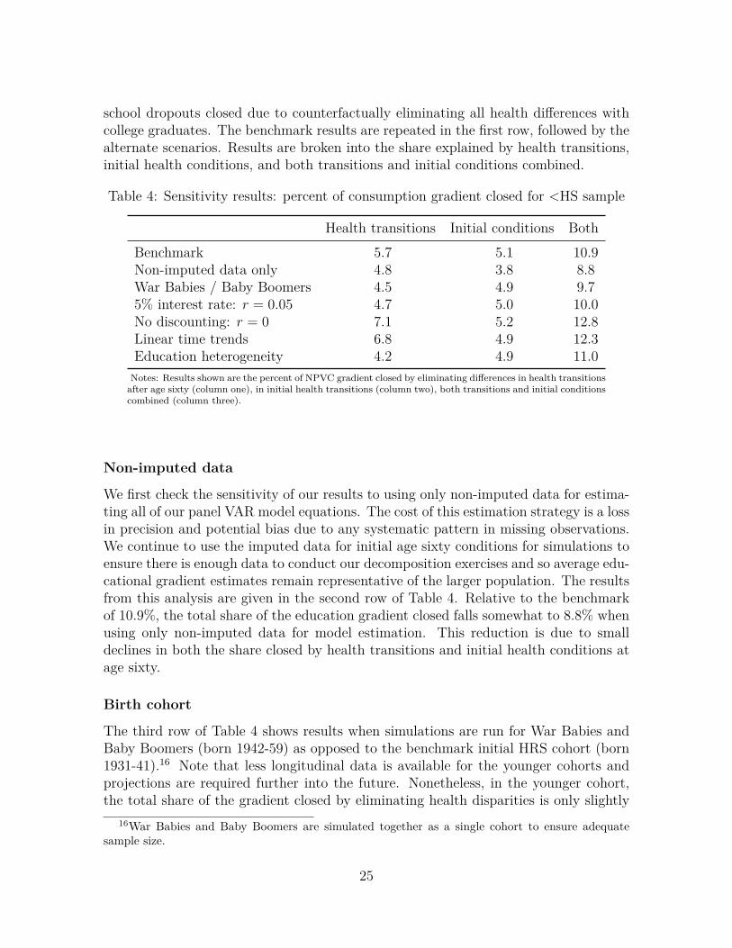
school dropouts closed due to counterfactually eliminating all health differences withcollege graduates. The benchmark results are repeated in the first row, followed by thealternate scenarios. Results are broken into the share explained by health transitions,initial health conditions, and both transitions and initial conditions combined.

Table 4: Sensitivity results: percent of consumption gradient closed for <HS sample

Health transitions Initial conditions BothBenchmark 5.7 5.1 10.9Non-imputed data only 4.8 3.8 8.8War Babies / Baby Boomers 4.5 4.9 9.75% interest rate: r = 0.05 4.7 5.0 10.0No discounting: r = 0 7.1 5.2 12.8Linear time trends 6.8 4.9 12.3Education heterogeneity 4.2 4.9 11.0Notes: Results shown are the percent of NPVC gradient closed by eliminating differences in health transitionsafter age sixty (column one), in initial health transitions (column two), both transitions and initial conditionscombined (column three).

Non-imputed data

We first check the sensitivity of our results to using only non-imputed data for estima-ting all of our panel VAR model equations. The cost of this estimation strategy is a lossin precision and potential bias due to any systematic pattern in missing observations.We continue to use the imputed data for initial age sixty conditions for simulations toensure there is enough data to conduct our decomposition exercises and so average edu-cational gradient estimates remain representative of the larger population. The resultsfrom this analysis are given in the second row of Table 4. Relative to the benchmarkof 10.9%, the total share of the education gradient closed falls somewhat to 8.8% whenusing only non-imputed data for model estimation. This reduction is due to smalldeclines in both the share closed by health transitions and initial health conditions atage sixty.

Birth cohort

The third row of Table 4 shows results when simulations are run for War Babies andBaby Boomers (born 1942-59) as opposed to the benchmark initial HRS cohort (born1931-41).16 Note that less longitudinal data is available for the younger cohorts andprojections are required further into the future. Nonetheless, in the younger cohort,the total share of the gradient closed by eliminating health disparities is only slightly

16War Babies and Baby Boomers are simulated together as a single cohort to ensure adequatesample size.

25

smaller (9.7%) than the older benchmark cohort. This decline is mostly driven by afall in the share closed by eliminating health transitions after age sixty.

Interest rate

The next two rows show the sensitivity of our results to the choice of interest rateused in calculating NPVC. The percent of NPVC gap closed is somewhat lower whenusing a higher discount rate of 5% compared to our benchmark rate of 3%. Thisdecline is primarily driven by a decline in the importance of health transitions asfuture realizations of outcomes are discounted more heavily. On the other hand, whenfuture consumption is not discounted at all, health transitions close 1.4 percentagepoints more of the consumption gap as compared to the benchmark, driving the totalgap closed up to 12.8%.

Time trend

In our model estimation, we do not allow for any innovations in health or growthin consumption, due to macroeconomic changes, past the final wave of the survey(2014). Here, we test the sensitivity of our results to allowing time trends in thefuture. Specifically, for the models of self-rated health, morbidities, and mortality, wereplace time dummies with a linear time trend that we assume continues past 2014.In the consumption model, replacing time dummies with a linear trend is empiricallymore problematic due to the timing of the great recession and subsequent recovery inrelation to the survey data. So we keep time dummies in the consumption equationbut assume that consumption grows at a rate of approximately 3% annually after 2014.As shown in Table 4, inclusion of linear time trends increases the share of the gradientclosed to 12.3%, primarily by increasing the importance of future health transitions.

Parameter heterogeneity across education groups

Our benchmark model also assumes homogeneity of all parameters across educationgroups. We relax this assumption by estimating the model separately for each of theeducation groups. This allows, for example, self-rated health to influence consumptiondifferently for high school versus college graduates. The cost of this approach is aloss in precision as the model is estimated entirely independently on education specificsub-samples. As shown in the last row of Table 4, combined results are very similarto the benchmark when incorporating heterogeneity in parameters along the educationdimension.

4 ConclusionWe estimated a panel VAR model using data from the Health and Retirement Study tounderstand the joint evolution of health and consumption at older ages. We used the

26

estimated model and empirical joint distribution at age sixty to simulate life-cycle pathsand construct a measure of the net present value of expected elderly consumption. Wefound an education gradient of $513,000 in NPVC between the college educated andhigh school dropouts at age sixty. In other terms, sixty year-olds with a college degreecould expect three times the remaining lifetime consumption of high school dropoutson average. We also estimated a life expectancy gradient of 5.4 years between theselevels of education at age sixty. Gradients were smaller but still substantial betweencollege and high school graduates—a 2.3 year gap in life expectancy and $324,000 inNPVC.

Counterfactual experiments indicated that two-year mortality transitions, condi-tional on current health, do little to explain the education gradient in consumptionamong the elderly. However, the differential evolution of self-rated health and mor-bidities could each close in the range of 2-3% of the consumption gaps between thecollege educated and lower attainment groups. Combined, we find that health andmortality transitions could close 5-8% of the gradients whereas the initial health distri-bution could close 4-5%. Taken together, we estimate that eliminating all elderly healthdifferences across education groups could close 11-12% of the education-consumptiongradient.

Our study is not without limitations. First, it is important to note that this isprimarily a descriptive analysis and we cannot make strong claims about causal in-ference. We cannot rule out selection into education categories and do not allow forany potential effect of elderly consumption on health. This type of reverse causalityor any other source of endogeneity could potentially bias our estimates of the effectof health evolution on consumption, hence our decomposition results. Moreover, ourcounterfactual experiments should be interpreted as the potential decline in the con-sumption gradient in response to an unexpected improvement in the health processesof elderly with less than a college degree. If counterfactual changes were anticipatedearly in life, there may also be endogenous changes in consumption patterns over theentire life-cycle. Finally, we do not allow for heterogeneities in medical innovationsover time. For instance, we do not account for the relative increase in survival due toimprovements in treatments for specific diseases like cancer. Another example wouldbe that we continue to assume the onset of diabetes has a time invariant effect on latentself-rated health. If future medical advances drastically lower the impact of diabeteson self-rated health, this change would not be explicitly captured. Nonetheless, ourstudy is an important first step towards understanding the role of health differences inexplaining consumption inequality. Addressing some of the aforementioned empiricalissues leaves room for important future research in this area.

ReferencesAguiar, M. and Bils, M. (2015). Has consumption inequality mirrored income inequa-lity? American Economic Review, 105(9):2725–56.

27

Attanasio, O., Hurst, E., and Pistaferri, L. (2014). The evolution of income, con-sumption, and leisure inequality in the United States, 1980–2010. In Improvingthe Measurement of Consumer Expenditures, pages 100–140. University of ChicagoPress.

Bloom, D. E., Canning, D., and Sevilla, J. (2004). The effect of health on economicgrowth: a production function approach. World development, 32(1):1–13.

Blundell, R. and Preston, I. (1998). Consumption inequality and income uncertainty.The Quarterly Journal of Economics, 113(2):603–640.

Born, B. and Breitung, J. (2016). Testing for serial correlation in fixed-effects paneldata models. Econometric Reviews, 35(7):1290–1316.

Case, A. and Deaton, A. (2017). Mortality and morbidity in the 21st century. Brookingspapers on economic activity, 2017:397.

Chetty, R., Stepner, M., Abraham, S., Lin, S., Scuderi, B., Turner, N., Bergeron, A.,and Cutler, D. (2016). The association between income and life expectancy in theUnited States, 2001-2014. JAMA, 315(16):1750–1766.

Conti, G., Heckman, J., and Urzua, S. (2010). The education-health gradient. AmericanEconomic Review, 100(2):234–38.

Cutler, D. M. and Katz, L. F. (1992). Rising inequality? Changes in the distributionof income and consumption in the 1980s. NBER Working Paper No. 3964.

Cutler, D. M., Katz, L. F., Card, D., and Hall, R. E. (1991). Macroeconomic perfor-mance and the disadvantaged. Brookings papers on economic activity, 1991(2):1–74.

Cutler, D. M. and Lleras-Muney, A. (2010). Understanding differences in health beha-viors by education. Journal of health economics, 29(1):1–28.

De Vos, I., Everaert, G., Ruyssen, I., et al. (2015). Bootstrap-based bias correction andinference for dynamic panels with fixed effects. Stata Journal, 15(4):986–1018(33).

Deaton, A. and Paxson, C. (1994). Intertemporal choice and inequality. Journal ofpolitical economy, 102(3):437–467.

Deaton, A. S. and Paxson, C. H. (1998). Aging and inequality in income and health.The American Economic Review, 88(2):248–253.

Dynarski, S., Gruber, J., Moffitt, R. A., and Burtless, G. (1997). Can families smoothvariable earnings? Brookings papers on economic activity, 1997(1):229–303.

28

Ettehad, D., Emdin, C. A., Kiran, A., Anderson, S. G., Callender, T., Emberson,J., Chalmers, J., Rodgers, A., and Rahimi, K. (2016). Blood pressure loweringfor prevention of cardiovascular disease and death: a systematic review and meta-analysis. The Lancet, 387(10022):957–967.

Everaert, G. and Pozzi, L. (2007). Bootstrap-based bias correction for dynamic panels.Journal of Economic Dynamics and Control, 31(4):1160–1184.

Goldman, D. P. and Smith, J. P. (2002). Can patient self-management help explain theses health gradient? Proceedings of the National Academy of Sciences, 99(16):10929–10934.

Griliches, Z. and Mason, W. M. (1972). Education, income, and ability. Journal ofpolitical Economy, 80(3, Part 2):S74–S103.

Heathcote, J., Perri, F., and Violante, G. L. (2010). Unequal we stand: An empiricalanalysis of economic inequality in the United States, 1967–2006. Review of EconomicDynamics, 13(1):15–51.

Honaker, J. and King, G. (2010). What to do about missing values in time-seriescross-section data. American Journal of Political Science, 54(2):561–581.

Houthakker, H. S. (1959). Education and income. The Review of Economics andStatistics, pages 24–28.

Hurd, M. D. and Rohwedder, S. (2007). Economic well-being at older ages: Income-and consumption-based poverty measures in the HRS. RAND Corporation WorkingPaper WR-410.

Idler, E. L. and Benyamini, Y. (1997). Self-rated health and mortality: A reviewof twenty-seven community studies. Journal of Health and Social Behavior, pages21–37.

Katz, L. F. et al. (1999). Changes in the wage structure and earnings inequality.Handbook of Labor Economics, 3:1463–1555.

Kenkel, D. S. (1991). Health behavior, health knowledge, and schooling. Journal ofPolitical Economy, 99(2):287–305.

Krueger, D. and Perri, F. (2003). On the welfare consequences of the increase ininequality in the united states. NBER macroeconomics annual, 18:83–121.

Krueger, D. and Perri, F. (2006). Does income inequality lead to consumption inequa-lity? evidence and theory. The Review of Economic Studies, 73(1):163–193.

Meara, E. R., Richards, S., and Cutler, D. M. (2008). The gap gets bigger: changes inmortality and life expectancy, by education, 1981–2000. Health Affairs, 27(2):350–360.

29

Miller, R. and Bairoliya, N. (2018). Health, longevity, and welfare inequality of theelderly. Working Paper.

Morgan, J. and David, M. (1963). Education and income. The Quarterly Journal ofEconomics, 77(3):423–437.

Mullahy, J. (2016). Estimation of multivariate probit models via bivariate probit. StataJournal, 16(1):37–51.

National Academies of Sciences, Engineering, and Medicine (2015). The growing gapin life expectancy by income: Implications for federal programs and policy responses.National Academies Press, Washington, DC.

Nickell, S. (1981). Biases in dynamic models with fixed effects. Econometrica,49(6):1417–1426.

Pijoan-Mas, J. and Ríos-Rull, J.-V. (2014). Heterogeneity in expected longevities.Demography, 51(6):2075–2102.

Shastry, G. K. and Weil, D. N. (2003). How much of cross-country income variation isexplained by health? Journal of the European Economic Association, 1(2-3):387–396.

Wursten, J. et al. (2016). Xtqptest: Stata module to perform Born & Breitung bias-corrected LM-based test for serial correlation. Statistical Software Components.

30

A Additional tables and figures

Table 5: Estimation sample descriptive statistics by highestlevel of education

<HS HS College

Individuals 11,396 17,971 6,515Observations 64,218 111,332 41,056Age (mean) 67.93 64.55 62.90Annual consumption ($1000s, mean) 16.34 25.60 40.79Hypertension (%) 55.08 48.71 41.45Diabetes (%) 21.88 15.57 12.25Cancer (%) 11.58 11.85 12.36Lung disease (%) 12.66 7.98 4.17Heart disease (%) 27.04 20.38 15.50Stroke (%) 10.58 6.74 4.57Psyche problem (%) 18.46 13.72 12.14Arthritis (%) 58.46 51.30 40.31Difficulty with ADLs (%) 36.31 21.25 13.07No Morbidities (%) 13.45 19.33 26.98Self-rated health (mean)Poor 16.39 6.63 3.19Fair 29.56 16.83 9.20Good 29.48 32.67 26.03Very good 18.22 31.68 39.69Excellent 6.35 12.18 21.89

Male (%) 44.09 40.61 53.44Race (%)White 76.50 88.44 89.89Black 15.74 8.21 5.52Other 7.76 3.34 4.58

Brith cohort (%)AHEAD 23.17 13.09 8.39CODA 14.76 10.85 9.42HRS 31.08 29.18 24.58War Babies 14.26 19.64 20.99Baby Boomers 16.74 27.24 36.62

Notes: Mean and percentage estimates use base year sampling weights. Con-sumption is reported in real 2010 dollars.

31

Table6:

Mod

elestim

ates

formorbiditie

sHyp

ertension

Diabe

tes

Can

cer

Lung

disease

Heart

disease

Stroke

Psych

Arthritis

Var

iabl

eCoeff

SECoeff

SECoeff

SECoeff

SECoeff

SECoeff

SECoeff

SESE

SE

LagHyp

er0.28

50.03

4-0.043

0.040

0.087

0.041

0.134

0.033

0.100

0.041

0.181

0.037

0.106

0.033

LagDiab

0.28

30.05

10.079

0.047

0.039

0.052

0.058

0.044

0.076

0.053

0.017

0.052

0.074

0.046

LagCan

cer

-0.017

0.05

20.02

20.05

40.088

0.060

-0.090

0.052

0.005

0.059

-0.004

0.060

0.052

0.052

LagLu

ng0.07

60.06

00.07

50.05

90.117

0.059

0.287

0.052

0.042

0.064

0.198

0.061

0.183

0.065

LagHeart

0.10

10.04

40.10

60.04

10.037

0.042

0.239

0.042

0.197

0.041

0.132

0.042

0.142

0.042

LagStroke

0.07

70.06

8-0.001

0.06

4-0.014

0.061

0.055

0.063

0.084

0.055

0.309

0.053

-0.024

0.063

LagPsych

0.113

0.05

40.09

10.05

3-0.064

0.060

0.136

0.056

0.144

0.048

0.194

0.054

0.275

0.055

LagArthritis

0.09

90.030

0.01

20.03

4-0.005

0.035

0.151

0.037

0.089

0.030

0.005

0.037

0.132

0.035

LagADL

0.09

20.03

30.07

20.036

0.010

0.035

0.199

0.035

0.118

0.030

0.238

0.033

0.320

0.032

0.197

0.037

Lag2

Hyp

er0.03

60.03

30.067

0.040

-0.062

0.040

0.050

0.033

0.060

0.041

-0.087

0.036

0.021

0.033

Lag2

Diab

-0.078

0.05

5-0.081

0.050

-0.073

0.055

0.125

0.046

0.094

0.055

0.068

0.055

-0.042

0.049

Lag2

Can

cer

0.00

20.05

6-0.003

0.05

80.038

0.064

0.122

0.055

-0.013

0.063

0.053

0.064

0.025

0.056

Lag2

Lung

-0.127

0.06

6-0.055

0.06

40.027

0.064

-0.086

0.058

0.054

0.069

0.007

0.066

-0.056

0.072

Lag2

Heart

-0.027

0.04

70.01

30.04

3-0.007

0.044

-0.046

0.044

-0.016

0.042

-0.040

0.044

-0.047

0.045

Lag2

Stroke

-0.027

0.07

70.019

0.07

00.020

0.067

-0.033

0.069

0.068

0.060

-0.196

0.059

0.037

0.070

Lag2

Psych

-0.045

0.05

8-0.069

0.05

70.064

0.064

0.049

0.060

-0.049

0.052

-0.051

0.058

-0.123

0.060

Lag2

Arthre

-0.044

0.03

00.012

0.03

40.057

0.035

-0.002

0.036

0.035

0.030

0.001

0.037

-0.007

0.034

Lag2

ADL

-0.073

0.03

60.04

10.03

80.003

0.038

-0.006

0.037

0.020

0.032

-0.088

0.035

-0.051

0.034

-0.068

0.042

CODA

-0.061

0.03

5-0.032

0.03

9-0.013

0.036

-0.033

0.041

-0.031

0.032

0.001

0.036

0.029

0.038

-0.166

0.036

HRS

-0.086

0.04

9-0.028

0.05

3-0.071

0.051

-0.096

0.057

-0.006

0.045

-0.029

0.052

0.030

0.054

-0.198

0.049

War

Bab

ies

-0.105

0.06

60.02

40.07

2-0.060

0.071

-0.107

0.080

0.035

0.063

0.051

0.075

0.152

0.075

-0.090

0.066

Boo

mers

-0.148

0.08

10.04

40.08

8-0.058

0.087

-0.115

0.099

0.082

0.078

0.059

0.093

0.301

0.092

-0.084

0.082

Black

0.20

90.02

20.110

0.02

1-0.026

0.022

-0.124

0.026

-0.104

0.020

0.067

0.024

-0.157

0.025

0.022

0.020

Other

race

0.048

0.03

20.23

30.03

4-0.195

0.044

-0.098

0.045

-0.095

0.036

-0.112

0.049

0.010

0.040

-0.044

0.033

Female

0.01

50.01

4-0.109

0.01

6-0.202

0.016

-0.076

0.018

-0.172

0.014

-0.066

0.017

0.123

0.017

0.149

0.014

HS

-0.077

0.01

6-0.123

0.018

0.023

0.018

-0.112

0.020

0.001

0.016

-0.000

0.019

-0.114

0.019

-0.034

0.017

College

-0.159

0.02

1-0.219

0.02

40.043

0.023

-0.284

0.029

-0.060

0.021

-0.060

0.027

-0.153

0.026

-0.081

0.021

Con

stan

t-1.561

0.06

6-2.065

0.07

5-2.080

0.077

-2.193

0.086

-2.023

0.068

-2.646

0.092

-2.262

0.078

-1.326

0.066

Not

es:Multivarite

prob

itresultswithdepe

ndentvariab

leacross

columns.Regressions

also

includ

edu

mmiesforag

ean

dyear.

32

Table 7: Model estimates ADLs, self-rated health, mortality, and consumptionADLs Self-rated health Mortality Consumption

Variable Coeff SE Coeff SE Coeff SE Coeff SE

Hyper 0.081 0.031 -0.273 0.015 0.083 0.027 -0.012 0.012Diab 0.172 0.040 -0.277 0.019 0.122 0.033 -0.036 0.018Cancer 0.114 0.044 -0.690 0.020 0.662 0.027 0.034 0.022Lung 0.326 0.048 -0.478 0.024 0.412 0.033 -0.008 0.027Heart 0.157 0.034 -0.496 0.017 0.178 0.025 -0.006 0.019Stroke 0.474 0.047 -0.501 0.023 0.238 0.030 -0.073 0.020Psych 0.449 0.044 -0.418 0.022 0.238 0.030 -0.088 0.017Arthritis 0.222 0.026 -0.214 0.015 -0.019 0.024 0.013 0.014ADL -0.673 0.014 0.343 0.020 -0.070 0.018Health 2 -0.335 0.017 0.061 0.019Health 3 -0.545 0.019 0.082 0.021Health 4 -0.666 0.023 0.117 0.021Health 5 (best) -0.657 0.033 0.147 0.025Lag Hyper -0.002 0.031 0.143 0.020 -0.034 0.027 -0.001 0.012Lag Diab 0.063 0.042 0.102 0.026 0.060 0.035 0.012 0.016Lag Cancer -0.058 0.047 0.547 0.029 -0.453 0.030 -0.009 0.023Lag Lung -0.022 0.053 0.210 0.034 -0.103 0.036 0.000 0.021Lag Heart -0.030 0.035 0.297 0.023 -0.018 0.026 0.007 0.018Lag Stroke -0.196 0.053 0.363 0.033 -0.047 0.033 0.004 0.019Lag Psych -0.124 0.047 0.233 0.031 -0.135 0.033 0.037 0.019Lag Arthre 0.093 0.026 0.119 0.018 -0.085 0.024 -0.011 0.013Lag ADL 0.340 0.018 -0.116 0.020 0.013 0.017Lag Health 2 0.630 0.014 -0.038 0.019 0.016 0.011Lag Health 3 1.139 0.015 -0.064 0.021 0.015 0.012Lag Health 4 1.668 0.016 -0.103 0.024 0.015 0.011Lag Health 5 (best) 2.290 0.019 -0.137 0.032 0.020 0.015CODA 0.032 0.028 0.019 0.015 -0.035 0.023HRS 0.002 0.041 0.022 0.021 -0.067 0.034War Babies 0.025 0.057 0.025 0.028 -0.131 0.051Boomers 0.146 0.070 -0.052 0.034 -0.099 0.062Black 0.154 0.018 -0.061 0.009 0.071 0.016Other race 0.118 0.032 -0.111 0.015 -0.065 0.031Female 0.006 0.013 0.031 0.006 -0.210 0.012HS -0.201 0.014 0.124 0.007 0.020 0.013College -0.317 0.019 0.236 0.009 -0.025 0.019Constant -1.620 0.058 1.696 3.310 -1.680 0.293Lag Con 0.173 0.005Lag2 Con 0.085 0.005

Notes: Dependent variable across columns. Multivariate probit results reported for ADLs as dependent outcome.Standard (ordered) probit results reported for self-rated health and mortality as dependant outcomes. Linear dynamicpanel estimates reported for consumption as outcome. All regressions also include dummies for age and year. Regressionfor self-rated health also includes second lag for all morbidities.

Table 8: Morbidity shock covariance matrix (Σ)Hyper Diabetes Cancer Lung Heart Stroke Psych Arthritis ADLs

Hyper 1.00 0.26 0.04 0.09 0.28 0.29 0.14 0.09 0.10Diabetes 0.26 1.00 0.07 0.06 0.10 0.14 0.06 0.03 0.09Cancer 0.04 0.07 1.00 0.12 0.03 0.06 0.12 0.05 0.13Lung 0.09 0.06 0.12 1.00 0.23 0.11 0.18 0.10 0.21Heart 0.28 0.10 0.03 0.23 1.00 0.28 0.17 0.11 0.16Stroke 0.29 0.14 0.06 0.11 0.28 1.00 0.22 0.11 0.41Psych 0.14 0.06 0.12 0.18 0.17 0.22 1.00 0.16 0.31Arthritis 0.09 0.03 0.05 0.10 0.11 0.11 0.16 1.00 0.26ADLs 0.10 0.09 0.13 0.21 0.16 0.41 0.31 0.26 1.00

33

.4

.6

.8

60 65 70 75 80 60 65 70 75 80 60 65 70 75 80

<HS HS College

Hyp

erte

nsio

n

Age

.1

.2

.3

.4

60 65 70 75 80 60 65 70 75 80 60 65 70 75 80

<HS HS College

Dia

bete

s

Age

.05.1

.15.2

.25

60 65 70 75 80 60 65 70 75 80 60 65 70 75 80

<HS HS College

Can

cer

Age

0

.1

.2

.3

60 65 70 75 80 60 65 70 75 80 60 65 70 75 80

<HS HS College

Lung

dis

ease

Age

Simulated Data

Figure 8: Mean of life-cycle morbidity profiles by educationNotes: “Data” plots mean of all available data (inclusive of imputed missing values) in HRS by two-year age intervaland cohort. “Simulated” plots mean of expected simulated outcome for each observation in the data (i.e. the expectedoutcome for each person-year observation in the data).

34

.1

.2

.3

.4

60 65 70 75 80 60 65 70 75 80 60 65 70 75 80

<HS HS College

Hea

rt di

seas

e

Age

0

.05

.1

.15

60 65 70 75 80 60 65 70 75 80 60 65 70 75 80

<HS HS College

Stro

ke

Age

.05

.1

.15

.2

.25

60 65 70 75 80 60 65 70 75 80 60 65 70 75 80

<HS HS College

Psy

che

prob

lem

Age

.4

.5

.6

.7

.8

60 65 70 75 80 60 65 70 75 80 60 65 70 75 80

<HS HS College

Arth

ritis

Age

Simulated Data

Figure 9: Mean of life-cycle morbidity profiles by educationNotes: “Data” plots mean of all available data (inclusive of imputed missing values) in HRS by two-year age intervaland cohort. “Simulated” plots mean of expected simulated outcome for each observation in the data (i.e. the expectedoutcome for each person-year observation in the data).

35

0

.2

.4

.6

60 65 70 75 80 60 65 70 75 80 60 65 70 75 80

<HS HS College

AD

L lim

itatio

n

Age

0

.1

.2

60 65 70 75 80 60 65 70 75 80 60 65 70 75 80

<HS HS College

Poo

r hea

lth

Age

0

.1

.2

.3

60 65 70 75 80 60 65 70 75 80 60 65 70 75 80

<HS HS College

Exc

elle

nt h

ealth

Age

0

.05

.1

60 65 70 75 80 60 65 70 75 80 60 65 70 75 80

<HS HS College

Mor

talit

y ra

te

Age

Simulated Data

Figure 10: Mean of life-cycle ADL limitation, self-rated health, and mortality profilesby educationNotes: “Data” plots mean of all available data (inclusive of imputed missing values) in HRS by two-year age intervaland cohort. “Simulated” plots mean of expected simulated outcome for each observation in the data (i.e. the expectedoutcome for each person-year observation in the data).

36

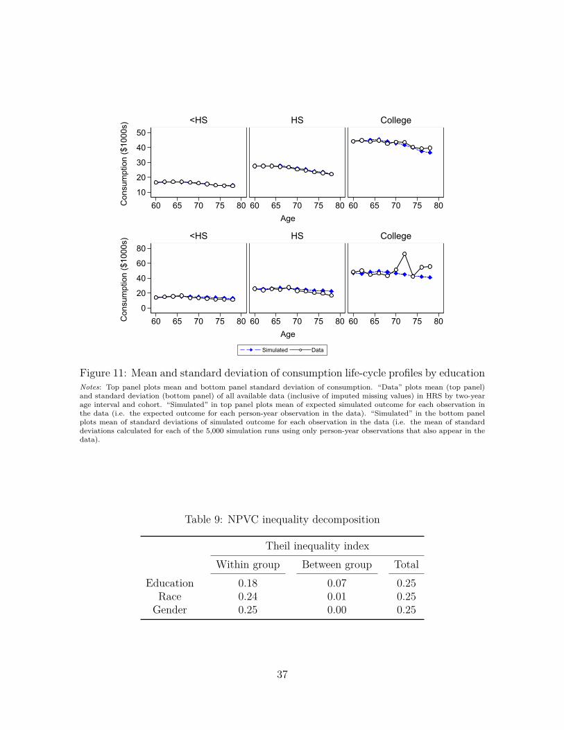
10

20

30

40

50

60 65 70 75 80 60 65 70 75 80 60 65 70 75 80

<HS HS CollegeC

onsu

mpt

ion

($10

00s)

Age

0

20

40

60

80

60 65 70 75 80 60 65 70 75 80 60 65 70 75 80

<HS HS College

Con

sum

ptio

n ($

1000

s)

Age

Simulated Data

Figure 11: Mean and standard deviation of consumption life-cycle profiles by educationNotes: Top panel plots mean and bottom panel standard deviation of consumption. “Data” plots mean (top panel)and standard deviation (bottom panel) of all available data (inclusive of imputed missing values) in HRS by two-yearage interval and cohort. “Simulated” in top panel plots mean of expected simulated outcome for each observation inthe data (i.e. the expected outcome for each person-year observation in the data). “Simulated” in the bottom panelplots mean of standard deviations of simulated outcome for each observation in the data (i.e. the mean of standarddeviations calculated for each of the 5,000 simulation runs using only person-year observations that also appear in thedata).

Table 9: NPVC inequality decomposition

Theil inequality indexWithin group Between group Total

Education 0.18 0.07 0.25Race 0.24 0.01 0.25

Gender 0.25 0.00 0.25

37