Health as an Informational Good:The Determinants of Child Nutrition andMortality During Political and Economic

Recovery in Uganda

WPS/95-9

John Mackinnon

March 1995

Centre for the Study of African Economies,University of Oxford,21 Winchester Road,Oxford, OX2 6NA.

Direct dial telephone number: +44 (0)1865 274550

Note: this project was financed by the Overseas Development Administration and I am grateful for their support. Iam most grateful to the Statistics Department, Entebbe for providing the data from the Integrated Household Surveyused in this paper and for much helpful discussion of it. All the statistics presented are based on the author'scalculations based on this data. Neither the ODA nor the Statistics Department are responsible for the views expressed.I am also grateful to colleagues at Oxford for helpful suggestions, especially Simon Appleton and Pip Bevan, and toa number of people who provided helpful advice in Uganda and Oxford, in particular Mr. Gupta, Jackson Kanyerezi,Tom Emwanu, Germina Ssemogerere, Arsene Balihuta, Achilles Sserwaya, Tom Barton, Jessica Jitta, Dan Mulder,Patrick Kadama, Abby Ssebina, Francis Mwesigye, and Joanna McRae. I am particularly grateful to Simon Appletonfor letting me use his poverty index. I would like to thank seminar participants at the University of Warwick and atthe Economic Policy Research Centre, Kampala. Responsibility for all errors is mine alone.

Abstract: Uganda suffers from a high rate of child mortality which has improved little if at all in the last twenty years.The paper uses data from the 1992 Integrated Household Survey to model the determinants of child mortality andmalnutrition. Parental beliefs about health have a strong and very highly significant influence on child mortality.Education and income also play a role, partly coming through its effect on beliefs, but early primary education seemsto have little effect.

1

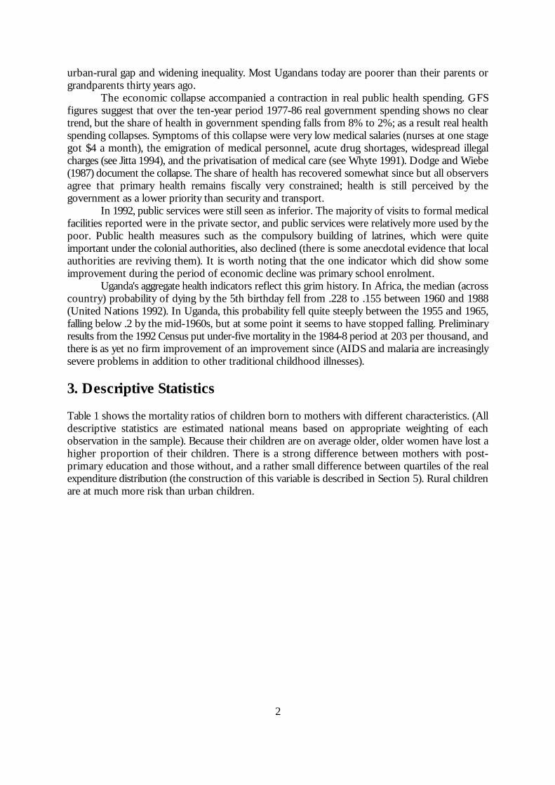
1. Introduction

Many children die avoidably. It is now widely understood, thanks in part to the experience of China,that public action can massively reduce mortality even when incomes remain low. However, manypoor countries are fiscally highly constrained; priorities within health and educational spending needto be examined carefully in order to see exactly what kind of action will save most lives. Manystudies find that education reduces mortality, but few existing economic studies explain why;moreover, most studies impose a linear or at best (Strauss 1990) a quadratic relation between yearsof schooling and health outcomes. Some studies include interesting interactions between educationand public services, and Thomas et al. (1991) examine the use that parents make of information asa determinant of child height they find that the effects of education mainly come through moreactive information-gathering behaviour (for instance, whether mothers read a newspaper or listento the radio).

The present paper uses data from Uganda, where child mortality (the probability of deathbefore the fifth birthday) is about 20% and has not fallen in twenty years, to shed more light on thechannels through which public action could affect child health. Unusually, both nutritional andmortality outcomes are modelled; mortality is modelled with more success. Child mortality turnsout to respond very strongly to parental beliefs about the causation of disease. Education and healthpractices also matter, but early primary education does not seem to make much difference. Use ofa very large sample of well-collected data overcomes the problem of multicollinearity which mightmake these hypotheses seem impossible to distinguish.

The policy implication is strong. To save children, parents need to know more about health.Education certainly has a role to play in this, but it need not be the only tool of public action andits quality may matter as much as its quantity. Also, the advocacy of market solutions for healthproblems needs to take massive informational failure into account.

Economists studying health have rarely collected or used data on beliefs (an exception isHaddad and Bouis 1990). But medical and anthropological studies provide evidence of theirimportance: see (among a large literature) Anokbonggo et al. (1990), Bukenya et al .(1990),Hilderbrand et al. (1985), Khan (1986), Linskog and Lundqvist (1989), and Pielemeier (1985). Forinstance, in Papua New Guinea Bukenya et al (1990) used very precise information on the beliefsand practices of a small sample of women; they were able to show that mothers' attitudes towardschild faeces, combined with the practice of sweeping the compound, were a critical determinant ofchild diarrhoea. Similar studies in Uganda are surveyed in Barton and Wamai (1994). However, mostof these studies do not construct an economic model and use more limited socioeconomicinformation than is provided by a household survey. The present paper seeks to develop a linkbetween the medical/anthropological and economic approaches.

2. Data and Context

The data analyzed in this paper come from the Ugandan Integrated Survey of 1992/3, conductedby the Statistics Department of the Ministry of Economic Planning and Development with WorldBank support as part of the Social Dimensions of Adjustment project, covering a sample of about10,000 households from all districts, and about 1,000 communities. The data were carefully collectedand checks on its quality are encouraging.

From 1972 to 1986, Uganda experienced two periods of severe political violence, thegovernment of Idi Amin which was overthrown by the Tanzanian army in 1979, and the civil warof the early 1980s which ended when the National Resistance Movement took power in 1986.Incomes collapsed and the economy retreated into subsistence. Although the economy grew from1986 to 1992 (when the data in this paper was collected) this probably accompanied a widening

2

urban-rural gap and widening inequality. Most Ugandans today are poorer than their parents orgrandparents thirty years ago.

The economic collapse accompanied a contraction in real public health spending. GFSfigures suggest that over the ten-year period 1977-86 real government spending shows no cleartrend, but the share of health in government spending falls from 8% to 2%; as a result real healthspending collapses. Symptoms of this collapse were very low medical salaries (nurses at one stagegot $4 a month), the emigration of medical personnel, acute drug shortages, widespread illegalcharges (see Jitta 1994), and the privatisation of medical care (see Whyte 1991). Dodge and Wiebe(1987) document the collapse. The share of health has recovered somewhat since but all observersagree that primary health remains fiscally very constrained; health is still perceived by thegovernment as a lower priority than security and transport.

In 1992, public services were still seen as inferior. The majority of visits to formal medicalfacilities reported were in the private sector, and public services were relatively more used by thepoor. Public health measures such as the compulsory building of latrines, which were quiteimportant under the colonial authorities, also declined (there is some anecdotal evidence that localauthorities are reviving them). It is worth noting that the one indicator which did show someimprovement during the period of economic decline was primary school enrolment.

Uganda's aggregate health indicators reflect this grim history. In Africa, the median (acrosscountry) probability of dying by the 5th birthday fell from .228 to .155 between 1960 and 1988(United Nations 1992). In Uganda, this probability fell quite steeply between the 1955 and 1965,falling below .2 by the mid-1960s, but at some point it seems to have stopped falling. Preliminaryresults from the 1992 Census put under-five mortality in the 1984-8 period at 203 per thousand, andthere is as yet no firm improvement of an improvement since (AIDS and malaria are increasinglysevere problems in addition to other traditional childhood illnesses).

3. Descriptive Statistics

Table 1 shows the mortality ratios of children born to mothers with different characteristics. (Alldescriptive statistics are estimated national means based on appropriate weighting of eachobservation in the sample). Because their children are on average older, older women have lost ahigher proportion of their children. There is a strong difference between mothers with post-primary education and those without, and a rather small difference between quartiles of the realexpenditure distribution (the construction of this variable is described in Section 5). Rural childrenare at much more risk than urban children.

3

Table 1: Ratio of Children who have Died

All women <20 21-5 26-30 31-5 36-40 >40

rural 0.24 0.12 0.15 0.18 0.20 0.20 0.31urban 0.17 0.09 0.11 0.13 0.15 0.17 0.27

Expenditure quartiles1st (low) 0.25 0.13 0.17 0.17 0.19 0.19 0.33 2nd 0.24 0.15 0.13 0.16 0.19 0.20 0.32 3rd 0.23 0.07 0.17 0.19 0.20 0.19 0.30 4th 0.22 0.11 0.13 0.16 0.19 0.20 0.30 Maternal educationNone 0.28 0.10 0.17 0.20 0.21 0.22 0.34 Some primary 0.19 0.11 0.15 0.16 0.20 0.18 0.25 Some secondary 0.10 0.04 0.08 0.11 0.09 0.14 0.11 Some further 0.07 0.00 0.03 0.07 0.05 0.08 0.09

Source: author's calculations from the 1992/3 Integrated Household Survey

Table 2 shows the proportion of children at different levels of nutritional status, measured in Z-scores (standard deviations from the mean of the reference population) of height-for-age: Table3 shows weight-for-height.

Table 2:Height-for-age: Z-scores

(calculated as distance from the mean of the international reference population,in terms of standard deviations of that population).

<-3 -3 to -2 -2 to -1 -1 to +1 +1 to +2 Above +2Total

male 23.0 20.7 24.2 24.7 4.5 2.8female 19.0 18.7 22.6 31.1 4.3 4.3

urban 13.4 15.3 25.3 36.0 6.9 3.1

rural 22.2 20.4 23.1 26.6 4.0 3.6

cont ...

4

Table 2 cont ...

<-3 -3 to -2 -2 to -1 -1 to +1 +1 to +2 Above +2Total

Expenditure quartiles1st (lowest) 23.0 21.2 21.5 26.0 4.8 3.52nd 22.7 19.3 23.4 27.0 4.1 3.43rd 20.1 20.2 24.8 28.2 3.5 3.24th (highest) 18.6 18.4 23.8 30.0 5.2 4.0

Age (years)

Boys0 13.4 22.1 26.7 31.4 4.0 2.31 29.4 24.8 20.7 18.0 4.3 2.82 23.9 18.9 22.0 24.8 4.8 5.53 23.1 18.9 24.5 26.2 4.4 2.74 23.3 19.6 27.6 24.0 5.0 0.5

Girls0 11.0 12.7 27.5 39.6 4.9 4.21 20.5 20.4 25.9 26.6 2.5 3.92 19.6 19.9 19.1 31.2 4.7 5.53 19.0 20.7 22.9 28.9 4.3 4.14 23.0 17.8 20.9 29.1 5.2 3.9

Maternal education

Illiterate 23.4 20.6 22.1 25.5 4.3 4.0Literate, incomplete prim 21.0 20.2 24.7 27.5 3.6 3.1Completed prim/some sec 17.0 17.6 22.6 32.9 6.1 3.8Completed further - 7.9 12.9 79.2 - -

Source: author's calculations from the 1992/3 Integrated Household Survey

Tables 2 and 3, which present data on nutrition, have a number of dramatic implications. First,overall levels of wasting in Uganda are not very far from the reference population (this can be seenfrom the fact that the distribution is nearly symmetrical around a Z-score of 0), but levels ofstunting are very high. Secondly, there is one age group where a high incidence of wasting isobserved, children between one and two years of age. Height-for-age also worsens dramaticallyduring the second year of life (a finer disaggregation shows deterioration from the age of sixmonths).

5

Table 3:Weight-for-height: Z-scores

(calculated as distance from the mean of the international reference population,in terms of standard deviations of that population).

<-3 -3 to -2 -2 to -1 -1 to +1 +1 to +2 Above +2Total

male 2.0 3.9 13.5 61.3 13.2 6.0female 1.5 3.6 15.0 60.8 13.1 5.9

urban 3.4 3.2 12.4 58.9 13.7 8.3rural 1.5 3.9 14.5 61.4 13.1 5.6

Expenditure quartiles1st (lowest) 1.9 5.4 17.2 60.9 10.4 4.22nd 2.0 4.8 14.2 60.5 12.9 5.53rd 1.6 3.0 13.3 64.2 13.6 7.24th (highest) 1.6 2.2 12.4 61.6 15.4 6.7

Age (years)

Boys0 3.1 3.4 8.9 48.3 20.6 15.61 1.7 7.1 20.9 49.8 14.7 5.62 2.0 2.9 10.9 70.1 11.5 2.53 2.3 2.3 13.1 67.5 11.7 3.14 1.0 4.1 13.2 65.2 10.4 6.9

Girls0 2.4 2.7 8.3 46.6 23.0 17.11 1.1 8.2 17.4 52.0 13.2 8.02 2.5 2.1 17.3 66.4 9.4 2.23 1.6 2.8 13.4 68.5 10.6 3.14 0.5 2.7 15.8 64.0 13.3 3.5

Maternal education

Illiterate 1.9 4.0 14.3 62.1 12.1 5.6Literate, incomplete prim 1.5 3.7 14.3 60.4 13.7 6.4Completed prim/some sec 2.3 3.5 13.9 60.2 14.3 5.9Completed further - - - 76.1 10.9 12.9

Source: author's calculations from the 1992/3 Integrated Household Survey

What this seems to suggest is that children in Uganda suffer a nutritional setback in the second yearof life which permanently reduces their height. Likely explanations include increased exposure todisease, a loss of the inherited immunity which shields children during the first few months, andinappropriate weaning foods. Food shortage at the level of the household seems a less plausibleexplanation for such an age-specific pattern of malnutrition (though the economic returns to thesurvival of a child from the household's point of view increase with the child's age, because of sunkcosts, and so we might expect food-scarce households to favour older children). However, the

6

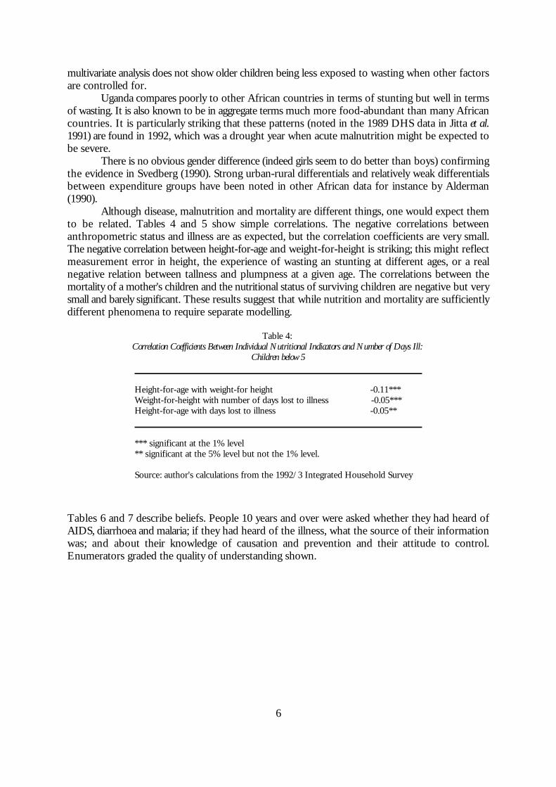
multivariate analysis does not show older children being less exposed to wasting when other factorsare controlled for.

Uganda compares poorly to other African countries in terms of stunting but well in termsof wasting. It is also known to be in aggregate terms much more food-abundant than many Africancountries. It is particularly striking that these patterns (noted in the 1989 DHS data in Jitta et al.1991) are found in 1992, which was a drought year when acute malnutrition might be expected tobe severe.

There is no obvious gender difference (indeed girls seem to do better than boys) confirmingthe evidence in Svedberg (1990). Strong urban-rural differentials and relatively weak differentialsbetween expenditure groups have been noted in other African data for instance by Alderman(1990).

Although disease, malnutrition and mortality are different things, one would expect themto be related. Tables 4 and 5 show simple correlations. The negative correlations betweenanthropometric status and illness are as expected, but the correlation coefficients are very small.The negative correlation between height-for-age and weight-for-height is striking; this might reflectmeasurement error in height, the experience of wasting an stunting at different ages, or a realnegative relation between tallness and plumpness at a given age. The correlations between themortality of a mother's children and the nutritional status of surviving children are negative but verysmall and barely significant. These results suggest that while nutrition and mortality are sufficientlydifferent phenomena to require separate modelling.

Table 4: Correlation Coefficients Between Individual Nutritional Indicators and Number of Days Ill:

Children below 5

Height-for-age with weight-for height -0.11***Weight-for-height with number of days lost to illness -0.05***Height-for-age with days lost to illness -0.05**

*** significant at the 1% level** significant at the 5% level but not the 1% level.

Source: author's calculations from the 1992/3 Integrated Household Survey

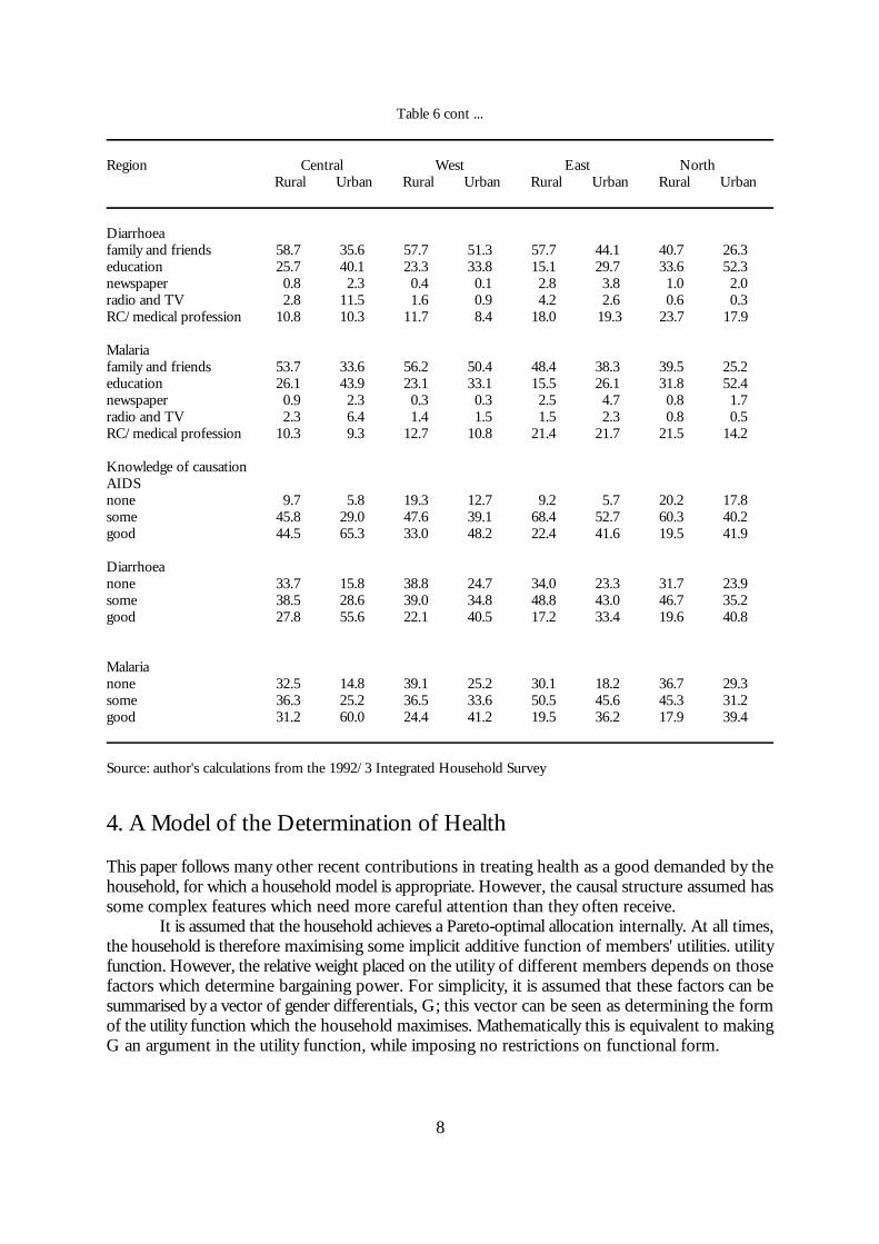
Tables 6 and 7 describe beliefs. People 10 years and over were asked whether they had heard ofAIDS, diarrhoea and malaria; if they had heard of the illness, what the source of their informationwas; and about their knowledge of causation and prevention and their attitude to control.Enumerators graded the quality of understanding shown.

7

Table 5:

Correlation Coefficients Between Ratio of Deceased Children and Average Indicators for Surviving Household Members under Five

Ratio of deceased children with mean weight-for-height -0.02Ratio of deceased children with mean height-for-age -0.03*Ratio of deceased children with mean days ill 0.01

* significant at 10% level

Source: author's calculations from the 1992/3 Integrated Household Survey

The vast majority of people had heard of all the illnesses, with family and friends the mainsource, followed by education (Table 6). Knowledge of causation was very similar to knowledge ofprevention (which is therefore not shown) and most people expressed an interest in control, ratherthan a fatalistic attitude. As expected, urban people are better informed than rural people. Table 7shows the relation between information, age and gender. There is a concave relation with age; thebest informed group are those between 26 and 45. There is no gap between the knowledge ofyoung boys and young girls, but as age increases a widening gender gap emerges. However, thisgender difference is not observed when men and women of the same educational level areconsidered.

Table 6:Beliefs about Illnesses, by Region

Region Central West East NorthRural Urban Rural Urban Rural Urban Rural Urban

Proportion who have heard of:AIDS 98.5 99.4 96.7 97.3 94.7 96.8 92.8 94.1Diarrhoea 90.8 95.3 90.1 87.3 88.8 87.8 94.1 92.4Malaria 93.5 95.6 93.8 96.1 90.2 93.1 94.7 94.1

Information source:AIDS family and friends 70.8 48.6 67.9 56.8 74.9 58.2 59.5 40.7

education 12.2 14.8 11.5 17.1 9.3 16.7 19.1 29.7newspaper/poster 3.1 6.8 2.5 3.9 3.6 6.5 3.5 12.9radio and TV 9.6 27.3 14.7 18.5 7.8 11.7 6.3 10.4RC/medical profession 3.9 2.5 3.4 3.7 4.2 6.6 11.4 6.2

cont ...

8

Table 6 cont ...

Region Central West East NorthRural Urban Rural Urban Rural Urban Rural Urban

Diarrhoeafamily and friends 58.7 35.6 57.7 51.3 57.7 44.1 40.7 26.3education 25.7 40.1 23.3 33.8 15.1 29.7 33.6 52.3newspaper 0.8 2.3 0.4 0.1 2.8 3.8 1.0 2.0radio and TV 2.8 11.5 1.6 0.9 4.2 2.6 0.6 0.3RC/medical profession 10.8 10.3 11.7 8.4 18.0 19.3 23.7 17.9

Malaria family and friends 53.7 33.6 56.2 50.4 48.4 38.3 39.5 25.2education 26.1 43.9 23.1 33.1 15.5 26.1 31.8 52.4newspaper 0.9 2.3 0.3 0.3 2.5 4.7 0.8 1.7radio and TV 2.3 6.4 1.4 1.5 1.5 2.3 0.8 0.5RC/medical profession 10.3 9.3 12.7 10.8 21.4 21.7 21.5 14.2

Knowledge of causationAIDS none 9.7 5.8 19.3 12.7 9.2 5.7 20.2 17.8some 45.8 29.0 47.6 39.1 68.4 52.7 60.3 40.2good 44.5 65.3 33.0 48.2 22.4 41.6 19.5 41.9

Diarrhoeanone 33.7 15.8 38.8 24.7 34.0 23.3 31.7 23.9some 38.5 28.6 39.0 34.8 48.8 43.0 46.7 35.2good 27.8 55.6 22.1 40.5 17.2 33.4 19.6 40.8

Malarianone 32.5 14.8 39.1 25.2 30.1 18.2 36.7 29.3some 36.3 25.2 36.5 33.6 50.5 45.6 45.3 31.2good 31.2 60.0 24.4 41.2 19.5 36.2 17.9 39.4

Source: author's calculations from the 1992/3 Integrated Household Survey

4. A Model of the Determination of Health

This paper follows many other recent contributions in treating health as a good demanded by thehousehold, for which a household model is appropriate. However, the causal structure assumed hassome complex features which need more careful attention than they often receive.

It is assumed that the household achieves a Pareto-optimal allocation internally. At all times,the household is therefore maximising some implicit additive function of members' utilities. utilityfunction. However, the relative weight placed on the utility of different members depends on thosefactors which determine bargaining power. For simplicity, it is assumed that these factors can besummarised by a vector of gender differentials, G; this vector can be seen as determining the formof the utility function which the household maximises. Mathematically this is equivalent to makingG an argument in the utility function, while imposing no restrictions on functional form.

E (U (D,C,H,L,G,HP) *B)

PC # w(E)L %Y

9

Table 7:Beliefs about Illness: by Sex and Age

Age 10-15 16-25 26-35 36-45 46-55 >55Sex M F M F M F M F M F M F

Knowledge of cause:AIDSnone 27.0 29.2 6.2 8.2 4.5 9.0 6.0 12.0 6.8 20.6 19.5 32.7some 57.4 54.0 52.7 52.7 48.2 50.1 50.1 52.6 55.9 53.9 54.4 49.9good 15.6 16.8 41.0 39.4 47.3 38.6 43.9 35.4 37.3 25.5 26.1 17.3

Diarrhoeanone 48.5 49.7 22.0 25.2 19.9 27.0 23.8 34.4 24.0 39.4 41.7 54.5some 39.0 38.3 45.8 44.2 42.7 44.7 40.5 40.3 44.9 44.0 40.6 36.0good 12.5 11.9 32.2 30.6 28.3 28.3 35.6 25.2 31.1 16.6 17.7 9.5

Malarianone 46.0 46.7 21.0 26.1 19.4 29.2 23.1 35.5 24.9 41.0 42.1 55.3some 39.0 37.9 43.2 41.9 41.1 42.6 39.8 37.8 41.0 42.0 40.6 34.5good 15.0 15.4 35.8 32.0 39.5 28.2 37.1 26.7 34.0 16.9 17.3 10.2

Source: author's calculations from the 1992/3 Integrated Household Survey.

Hence the household maximises its expectation of a utility function given by

(1)

Here D is a vector of demographic variables; C is consumption; H is health; and L is laboursupplied to the market. HP is a vector of health practices; the practice of hygiene is assumed toaffect utility directly, for instance by requiring inputs of non-marketed labour, but the way in whichit does so is left flexible.

G is represented in what follows by including community-level data on male-femaledifferentials in the labour market (wages and job availability), because an improvement in the femaledifferentials will increase female bargaining power and hence probably improve child health.However, an alternative possibility is that an increase in female wages will draw female time out ofchild care. (It is hard to find a usable variable which captures effects on relative bargaining powerwithout also affecting allocation through relative prices: Thomas (1991) in Brazil uses unearnedfemale income, but this depends on the existence of state pensions. An alternative, not exploredhere, is the share of female income; however, if this is regarded as endogenous, the search forinstruments raises the same problems). Finally, the subjective expectation of utility is conditionalon the beliefs of household members about illness, B. Note that the maximisation is modelled astaking place ex ante, i.e. before the random component of illness is known.

(1) is maximised subject to the constraints in (2) to (5):

(2)

H ' f(HG,HP,V) % e

C # C

L # L

C ' C (P,w,Y,E,D,G,B,C,L)

HP ' HP (P,w,Y,E,D,G,B,C,L)

H ' H (P,w,Y,E,D,G,B,C,L,V) % e

10

Here Y is unearned income; C is the consumption vector; w is a vector of wage rates which areassumed to depend on the vector of educational levels E; and L is labour supplied to the market.This form of budget constraint assumes either that there is no subsistence production or that thefamily farm can be modelled as a price-taker in labour and product markets which buys family andoutside labour indifferently. While this assumption is not true in Uganda (see Appleton andMackinnon 1995), the crucial separability in what follows is between production and child health,and this seems a reasonable approximation. Separability between adult health and production wouldbe more problematic, though Pitt and Rosenzweig (1985) find it an acceptable approximation inIndonesia.

(3)

Here health depends in a stochastic fashion on vectors of marketed health goods, HG; these area subset of consumption C and would include both food and medical services: on HP, healthpractices within the household, and on V, a vector of environmental variables.

(4)

and

(5)

(4) and (5) represent quantity constraints on consumption, notably of health services, and onmarketed labour supply. Note that since the model can be interpreted intertemporally, the quantityconstraints may include a liquidity constraint; this justifies the use of data on informal insurance asa determinant of demand.

The maximisation problem yields demand functions for goods and services as follows:

(6)

(7)

These demand functions and the health production function (3) yield the reduced form model ofhealth:

(8)

The presence of education in the reduced form is justified, in the above argument, by its effect onthe budget constraint (2). There are, however, a number of alternative interpretations of thecoefficient of education in the reduced form. (a) Education affects the relative bargaining strengthof men and women. In this case the signs of female and male education should be opposite. (b)Education directly inculcates habits connected with health practices such as hand-washing. (c)Children's education affects the household's returns to successfully rearing them. All these effects,in the current model, could be represented by making education an argument in the utility functionand hence in the reduced form. (d) Education affects the cost of parental time. Finally, (e)education may affect beliefs; however, if beliefs are adequately measured, this should be picked upby the coefficient on beliefs and does not warrant the inclusion of education in the reduced form

11

one beliefs are included. However, education is in practice likely to pick up some information aboutany unobserved component of beliefs.

In the estimated model, it is assumed that income in (2) and child health are separable, sothat permanent income can be treated as an exogenous variable. Thus Y (unearned income) andE can be replaced in the reduced form by permanent income. For adult health, this would raiseproblems of exogeneity, but for children's health it seems reasonable. Permanent income is thenproxied by current expenditure and by indicators of housing quality - the number of rooms in thehousehold and whether the dwelling is self-standing. Reasons for not instrumenting income withassets (as is often done) are discussed in the next section. The use of income, rather than assets,removes the primary justification for including education in the reduced form, which was thateducation confers the power to earn income. However, the other justifications listed under (a) to(e) in the last paragraph remain plausible; hence it seems reasonable to retain education in thereduced form.

The vector of environmental variables V includes the prevailing forms of sanitation, waterand garbage disposal in the community. However, the exogeneity of these variables is not altogetherclear since the choices prevailing in the community reflect the choices of people in the sample. Atthe same time, individual health practices might themselves be exogenous if, for instance, latrinebuilding is compulsory. Moreover, it is of interest to find out how much of the influence of beliefsand education is coming through identifiable health practices. In view of these difficult issues ofcausal structure, four versions of each model are estimated: with beliefs, education and community-level practices: with beliefs, education and individual-level data on practices: with education andbeliefs: and with only education. A very similar approach to the (slightly different) problem ofmodelling education and information use is taken by Thomas et al. (1991).

A further possible problem of endogeneity concerns beliefs, since one would expect parentswhose children have died from a particular condition to have acquired some knowledge as a result.This could produce a spurious negative correlation between beliefs and health. However, the verystrong positive link actually found suggests that this form of endogeneity is not important.

5. Measurement Issues

Health is measured by the survival ratio of children ever born and two standard anthropometricmeasures, height-for-age and weight-for-height. The survival ratio is of acute intrinsic interest and,with the exception of paediatric AIDS where mothers may not long survive their children, isprobably fairly well measured. It has the drawback that observations on current clauses ofexplanatory variables are being used to explain past events. The anthropometric measures do referto current or recent events, but they are probably measured with more error than mortality, aresubject to possibly insignificant short-run fluctuations, and are of less intrinsic interest thenmortality.

Income was measured, as mentioned above, by real expenditure and by the quality ofhousing (number of rooms in the dwelling, and whether the household is self-contained). Themeasure of real expenditure was constructed for this dataset by Appleton (1994); regional povertylines were calculated based on the cost of a food basket, and expenditure per adult equivalent usingthe following scales was divided by the poverty line to get real expenditure per adult equivalent. Themeasure of housing quality raises the problem that it might be a direct input into the healthproduction function, since malaria in particular may well be carried between people sleeping in thesame room. The possibility of instrumenting permanent income with assets (widely used in theliterature) was rejected partly because the most important asset, land, may not be exogenous (wehave information on land used rather than land owned, and land in some parts of Uganda seemsto be 'lent' on criteria of need or personal loyalty): partly because land is missing for a number of

12

households, especially many urban households: and partly because the relation with land is complex;those with no land at all are better off that those with a little land (for more discussion see Appletonand Mackinnon 1995).

The use of a per-adult equivalent measure, whether of income or assets, raises problems ofendogeneity, since the denominator of such a measure is automatically reduced by the death of achild. One solution would be to regress separately on income and household size; but this wouldlead to a confusion between the cost effects of household size and other effects of varyingdemographic structure. On balance, the use of real expenditure per adult equivalent seemed thesimplest and most satisfactory available measure.

Education is measured by separate dummies on each grade achieved, allowing completefreedom in the functional form of the relation between years of schooling and health. Oneimportant caveat is selectivity bias; the attainment of a limited level of education may reflect the factthat the person has dropped out and hence be an indicator of low ability or discipline. In theequations for nutrition, parental education was used; the data here is less finely disaggregated.

The data on beliefs were discussed in Section 3; dummies for 'good' and 'some'understanding of the causation of diarrhoea and malaria were used. Paediatric Aids is likely to berelatively unimportant among children of surviving mothers.

A selection of prices for major food items, divided by the regional poverty line, was used;also, charges for some medical services were included. The vector of quantity constraints is proxiedby variables which measure the availability of services and markets, and by variables in thecommunity questionnaire on whether long-term support and short-support is available tohouseholds in dire need. The availability of services was measured by the distance from the nearestclinic and the nearest hospital and the presence of a nurse and a doctor in the nearest clinic.

Health environment was measured by the health practices (form of sanitation, water andgarbage disposal prevalent in the community, and mean age at weaning and the presence of anursery) and also by the prevalence of fuelwood as the main energy source (this may have a directimpact on children's respiratory systems). As noted above, the community variables on sanitation,water and garbage were used only in one version of the models; in another version household-leveldata was used instead. Also, a vector denoted by 'Practices' includes the average age at weaning andthe number of meals for adults and children; this turned out not to be significant in any model(perhaps because extended breastfeeding is almost universal in Uganda).

A full list of the variables used is given in Table 8. The focus on the mortality equations ison the mother, whereas in the nutrition equations it is on the particular child; so there are somedifferences between the equations. Also, nutrition is assumed to have a seasonal component.

In a significant proportion of cases, the data do not allow a household to be preciselymatched with a community. Rather than halving the sample size or omitting the very valuablecommunity data, a dummy was used for missing observations on particular variables and therelevant variable set to an arbitrary constant in these cases. The effect of this is to remove anyinfluence of these observations on the coefficient on the missing variable, while retaining the otherinformation from the observations.

13

Table 8:Variables Used in the Nutrition Equations

WHZ Z-score, weight-for-heightHAZ Z-score, height-for-ageONE etc. dummy for age of child (12-17 months)ONE5 etc. dummy for age of child (18-23 months)SEX =0 if male, 1 if femaleWELFARE spending per equivalent adult/regional poverty lineWELFSQ WELFARE squaredNROOMS number of roomsINDDWELL =1 if independent dwelling, 0 otherwiseGCHILD =1 if grandchild of head of householdSERVANT =1 if servantNOTREL =1 if not related to head of householdKIDRATIO proportion of children in householdKIDORDER =1 if oldest child in household, 2 if second, etc.FEB92 etc. seasonalFLIT/MLIT father/mother literate but no educationFPRIM/MPRIM father/mother had lower primary education (but no more)FP7/MP7 father/mother had upper primary educationFSEC/MSEC father/mother had lower secondary education (but no more)FALEVEL/MALEVEL father/mother had A-levelsFFUR/MFUR father/mother had further educationMALEMAL/FEMMAL average score for males/females in HH on knowledge of malaria

causation (2=good, 1=some 0=none)MALEDIA/FEMDIA average score for males, diarrhoea causationURBAN =1 if urbanEAST etc. regionRMATPR matooke priceRMZPR maize priceRCASPR cassava priceRPOTPR sweet potato priceRMILPR millet priceRMLKPR milk priceRBFPR beef priceRBNPR bean priceRSOPPR soap priceRASPPR aspirin priceFMFARMW ratio of female/male farm wage MFARMW male farm wageMALPRICE price of malaria drugs in clinicANTPRICE price of antibiotics in clinicCONSPRIX consultation fee in clinicDISTCLIN distance to clinicSUPPLIES =1 if regular supplies to clinicDOCTOR =1 if doctor regularly presentNURSE =1 if nurse regularly presentHOSPCOST cost of hospital stayGOVHOSP =1 if hospital is government-ownedINGOHOSP =1 if hospital is run by international NGOLNGOHOSP =1 if hospital is run by local NGO

cont ..

14

Table 8 cont ...

TAP =1 if main water supply is tap (Community)HTAP etc. =1 if main water supply is tap (Household)VENDOR main water supply vendor RAIN main water supply rainPWELL main water supply protected wellNPWELL unprotected wellCOLLECT rubbish collectedBURN rubbish burntBURY rubbish buriedMANURE rubbish used as green manureBUCKET main form of toilet a bucketFLUSH main form of toilet a flushLATRINE main form of toilet a latrineSSUPPORT support available in short termLSUPPORT support available in short termNURSERY nursery availableWEANAGE usual age at weaningADMEALS usual number of meals for adultsCHMEALS number of extra meals for childrenWOOD =1 if wood the main source of fuelAVAILDIF index for female-male differential in job opportunitiesAVAIL index for male job opportunitiesDISTCMKT distance to nearest consumer marketDISTMMKT distance to main consumer marketDISTTRAD distance to traderDISTPMKT distance to product marketNO... dummies for missing observations on particular variables

Additional variables in the mortality equation:RATIO ratio of children who have died to children ever bornAGE age of womanEDUC1 educated but 1st grade not completedEDUC11-1 primary grade 1-7 completedEDUCJUN junior schoolingEDUCSEC secondary schoolingEDUCFUR further educationBIRTHG female birthsBIRTHB male birthsGOODDIA good knowledge of diarrhoea causationSOMEDIA some knowledge of diarrhoea causationGOODMAL good knowledge of malaria causationSOMEMAL some knowledge of malaria causationSINGLE =1 if singleCOHABHH =1 if unmarried cohabiting with household headCOHABOTH =1 if unmarried cohabiting with otherDIVORCE =1 if divorcedWIDOW =1 if widowHEAD =1 if household headOTHREL =1 if relative other than child, grandchild, wife or servant of household

headWIVES number of wives of household head in the household

15

6. ResultsA general model was estimated in four versions for each dependent variable. For simplicity, OLSwas used for the estimation of mortality at this stage. In each model, block F-tests were used ongroups of variables to simplify the models. Tables 9 to 11 show the F-tests in each model. Themodels were then simplified using F-tests to justify the deletion of blocks of variables at each stage.Tables 12, 14 and 15 show the models finally selected, and Table 13 shows a variant of the modelsfor mortality concentrating on married couples to test for the flow of information within thehousehold. Because hypothesis-testing, rather than prediction, is the purpose of the modellingexercise, even the simplified models are large (also further restrictions were rejected by block F-tests).

Mortality is more satisfactorily modelled than nutrition; the hypothesis tests turn out to bemore powerful for mortality than for nutrition. The differences in results between the equations,discussed below, may reflect the differences in date of the events being explained or differencesbetween the phenomena of malnutrition and mortality; it is very hard to distinguish these in a cross-section data set. What is clear is that weight-for-height seems to respond most to short-termfactors, as one would expect on either view. Weight-for-height is more satisfactorily modelled thanheight-for-age, somewhat surprisingly.

The block F-tests for mortality, as well as the coefficients in the simplified model, show thatmortality, show very clearly that beliefs have a strong causal role even when conditioning oneducation and on community-level or household-level practices. Moreover, the coefficients are high.Note that about half the observations of mortality are censored at 0 or 1 (4912 were censored at0 and 298 at 1), so that the effect of improvement in knowledge on mortality is only about half thesize of the coefficients. Compared to the control group of mothers with no understanding of thecausation of malaria and diarrhoea, mothers with good knowledge have a reduced mortality ratereduced by roughly (.07+.02)/2=.045 ; this compares with an average mortality rate of about .2 andrepresents a very significant improvement as a result of increased understanding.

In Table 13, the sample is restricted to spouses of the household head (to avoid possiblyperverse effects from the death of a spouse on the measure of male education and beliefs) to testfor differential effects of beliefs and education of men and women. It turns out to be difficult todistinguish effects by gender; high multicollinearity is not surprising, given that spouses may havebeen interviewed together. So whereas we can be sure that beliefs do matter, it is not clear from thisdataset that women's beliefs matter more than men's.

Education also matters in explaining mortality and height-for-age. However, primaryeducation has relatively weak effects; it becomes significant in explaining mortality only when weremove practices from the equation, and more so when beliefs are removed (see the relevant lineof Table 9). This may suggest that the effects of primary education come mainly through beliefs andpractices (though the coefficients on education do not change much across the four versions of themodel in Table 12). Also, the coefficients on particular grades show that there is no strong evidenceof any beneficial effect of education until about the fifth grade of primary schooling. It would beuseful to understand more about exactly what is being taught in schools at different grades (Strauss1990 reports rather similar results in Cote d'Ivoire). The results help to explain why the increase inenrolment rates during a period of economic disruption did not deliver any improvement inmortality.

Practices associated with sanitation, water source and garbage disposal matter more forcurrent nutrition than for past mortality. Some of these variables, for instance the dummy forhaving garbage collected, may pick up unmeasured aspects of wealth. Since practices are measuredcurrently and may change more over time than beliefs, it is understandable that they should bemore powerful in the nutrition than the mortality equations. (The control groups are householdsor communities which have no toilet, dump their garbage at will, and get their water from the river).

16

The coefficients have the expected signs and are quite large. The use of fuelwood as the mainsource of energy at a community level worsens health outcomes; once again, this might be ameasure of wealth at the community level, but it may also reflect a direct effect on health.

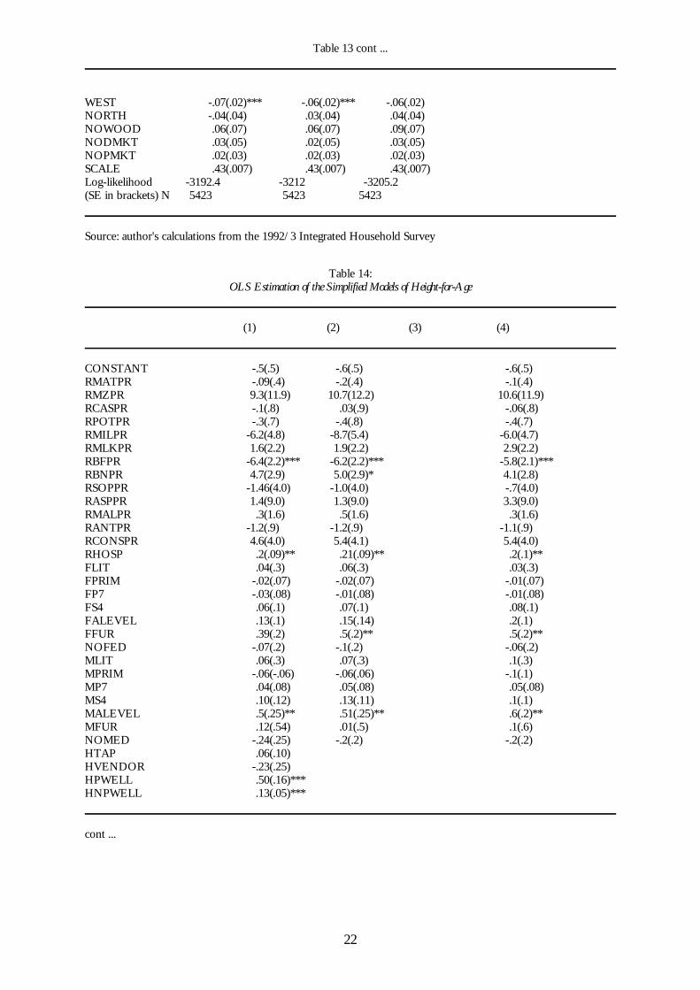
Economic status, measured by real expenditure and housing, matters in most cases. Thelong-run indicator, the number of rooms in the house, affects mortality (as noted above this couldreflect a direct environmental effect) whereas weight-for-height responds to the short-run indicator,real expenditure (WELFARE). The effects of expenditure they seem to be concave (so that a moreequal distribution would improve health) but the quadratic term is not significant in most cases.Similarly, relative food prices matter only in the equations for weight-for-height (they becamesignificant in block F-tests as the size of the model was reduced), though even here manycoefficients are insignificant and price effects do not seem to be very convincingly modelled,perhaps because observations are missing in many cases.

Gender differentials in the labour market were not found to be significant (as noted above,their sign is theoretically ambiguous but higher female wages were expected to benefit child health).However, the sex of the child does matter, both in mortality (where the coefficient on BIRTHBis much bigger than that on BIRTHG) and in weight-for-height; girls do better than boys. The ageof the child matters as expected for nutrition, but in contrast to the bivariate data presented earlierthere is no sign that weight-for-height is worse in the second year of life than in subsequent years.The reason for this is not clear. The marital status of the mother matters a great deal for mortality;children from polygamous households, or whose mothers are divorced or widowed, are at muchgreater risk (though some of these variables might be endogenous). The relations of children to thehousehold head, however, do not show specific problems for children who are not being lookedafter by their parents; this is of great interest given the large number of orphans in the population.It is often anecdotally suggested that orphans are discriminated against within the household; theseresults do not support this view. However, orphans do suffer because their mothers are widowed,and they may suffer when their mothers die because they move to poorer households.

Some aspects of services do seem to matter, more for nutrition than for mortality. Inparticular, the presence of a doctor has a powerful positive effect on weight-for-height. Prices forservices, in some cases, seem to have perverse effects; there is no support here for the view thatuser charges are damaging to health. However, the official prices reported in the dispensary maybe a poor proxy for actually imposed charges. Isolation has a perverse beneficial effect; distancefrom traders and from the main market seems to improve nutrition, It is possible this reflects aconflict between commercialisation and nutrition, but this suggestion is highly tentative. Thepresence of short-term support does seem to benefit the short-term nutritional indicator, weight-for-height.

In the nutrition equations, season is highly significant as a block (even though none of thet-ratios are significant) and the coefficients show a clear pattern across the year of the survey. Thismay reflect either a normal seasonal pattern or the drought which was at its worst in mid-to-late1992.

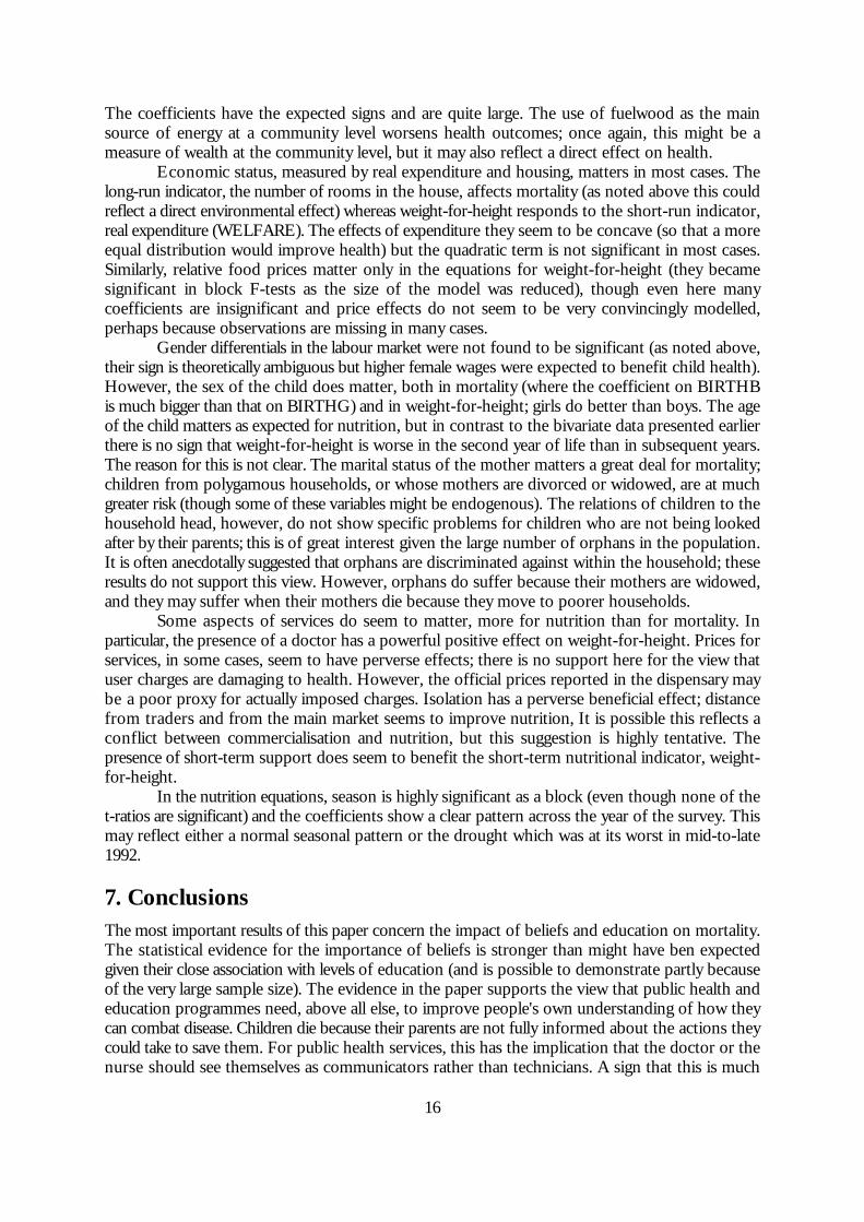
7. ConclusionsThe most important results of this paper concern the impact of beliefs and education on mortality.The statistical evidence for the importance of beliefs is stronger than might have ben expectedgiven their close association with levels of education (and is possible to demonstrate partly becauseof the very large sample size). The evidence in the paper supports the view that public health andeducation programmes need, above all else, to improve people's own understanding of how theycan combat disease. Children die because their parents are not fully informed about the actions theycould take to save them. For public health services, this has the implication that the doctor or thenurse should see themselves as communicators rather than technicians. A sign that this is much

17

misunderstood is the widespread observation, in a number of African countries, of very shortconsultation times (often associated with extravagant drug prescriptions). It also suggests that thereis potentially an enormous role for carefully designed public awareness campaigns. In the case ofAIDS, public awareness of the existence of the disease is almost universal and this certainly reflectspublic action to some extent.

Secondly, the results suggest that although education is a powerful way of increasingpeople's understanding, early primary education has in the past not succeeded in achieving verymuch benefit. Whether this reflects curriculum design, quality of schools, or the intrinsic difficultyof communicating complicated concepts such as the germ theory of disease in early primaryeducation, is hard to say. The Ugandan authorities are acting on the design of the curriculum,including health education at an early stage for both sexes; the results here strongly support thispolicy. Educational policymakers also need to think about exactly what a person needs tounderstand in order to protect their children, or themselves, from disease. To understand health,we need to understand information.

Table 9:Levels of Significance of Block F-tests in the General OLS Model of Mortality

(1) (2) (3) (4)

Food prices .8 .31 .81 .88Medical prices .11 .12 .08* .10*Education .0001*** .0002*** .0001*** .0001***Primary education .07* .16 .06* .02**Beliefs .0001*** .0001*** .0001*** .0001***Facilities .17 .13 .11 .09*Water (household) .6Garbage (household) .24Toilet (household) .08*Water (community) .11Garbage (community) .02**Toilet (community) .23Support .55 .41 .50 .37Weaning and meals .75 .82Job market .08* .10 .10* .14Gender differentials .59 .38 .21 .21Distance .12 .06* .09* .05*Economic status .0001*** .0001*** .0001*** .0001***Relations .0001*** .0003*** .0001*** .0001***Region .06* .03** .01** .01**

Note: the numbers in each cell give the probability of observing as high an F-statistic under the null that the group ofvariables has no influence on mortality*** significant at the 1% level; ** significant at the 5% level * significant at the 10% levelSource: author's calculations from the 1992/3 Integrated Household Survey

18

Table 10:Levels of Significance of Block F-tests in the General OLS Model of Height-for-Age

(1) (2) (3) (4)

Food prices .04** .02** .03** .03**Medical prices .09* .08* .09* .08*Father's education .38 .25 .19 .19Mother's education .32 .27 .20 .16Parental education .08* .03** .01*** .005***Beliefs, both .81 .83 .81Male beliefs .74 .81 .82Female beliefs .53 .55 .52Facilities .49 .44 .35 .36Water (household) .01**Garbage (household) .14Toilet (household) .004***Water (community) .07*Garbage (community) .22Toilet (community) .01**Support .71 .47 .41 .41Weaning and meals .59 .55Job market .31 .46 .34 .34Gender differentials .13 .17 .27 .26Distance .83 .96 .87 .85Economic status .00*** .0001*** .0001*** .0001***Region .01** .008*** .009*** .008***Relations .02** .04** .03** .03**Season .04** .21 .02** .02

Note: the numbers in each cell give the probability of observing as high an F-statistic under the null that the group ofvariables has no influence on height-for-age*** significant at the 1% level; ** significant at the 5% level *significant at the 10% levelSource: author's calculations from the 1992/3 Integrated Household Survey

Table 11:Levels of Significance of Block F-tests in the General OLS Model of Weight-for-Height

(1) (2) (3) (4)

Food prices .20 .17 .19 .16Medical prices .04** .03** .02** .02**Father's education .82 .83 .80 .89Mother's education .08* .08* .10 .13Parental education .25 .27 .32 .49Beliefs, both .01** .01** .01**Male beliefs .07* .06* .05**

cont ...

19

Table 11 cont ...

(1) (2) (3) (4)

Female beliefs .42 .43 .48Facilities .02** .03** .02** .03**Water (household) .04**Garbage (household) .08*Toilet (household) .86Water (community) .03**Garbage (community) .001***Toilet (community) .003***Support .07* .13 .06* .05*Weaning and meals .42 .51Job market .28 .31 .15 .12Gender differentials .51 .45 .49 .47Distance .02** .04** .01** .01**Economic status .27 .44 .11 .04**Region .0001*** .00*** .00*** .00***Relations .0009*** .00*** .00*** .00***Season .02** .01** .02** .01**

Note: the numbers in each cell give the probability of observing as high an F-statistic under the null that the group ofvariables has no influence on weight-for-height*** significant at the 1% level; ** significant at the 5% level *significant at the 10% levelSource: author's calculations from the 1992/3 Integrated Household Survey

Table 12:Tobit Estimation of the Simplified Models of Mortality

(1) (2) (3) (4)

CONST -.35(.04)*** -.34(.04)*** -.4(.04)*** -.4(.06)***EDUC1 -.02(.06) -.05(.07) -.02(.06) -.02(.06)EDUC11 .06(.04) .06(.05) .06(.04) .06(.04)EDUC12 .006(.05) .03(.03) .004(.03) .002(.026)EDUC13 .039(.02)* .02(.03) .037(.023) .032(.023)EDUC14 -.02(.02) -.03(.03) -.026(.022) -.033(.022)EDUC15 -.046(.02)** -.06(.03)** -.048(.022)** -.06(.022)***EDUC16 -.01(.02) -.003(.03) -.012(.02) -.027(.02)EDUCJUN -.22(.08)*** -.19(.10)** -.22(.08)*** -.25(.08)***EDUCSEC -.14(.02)*** -.14(.03)*** -.15(.025)*** -.17(.02)***EDUCFUR -.24(.04)*** -.23(.04)*** -.25(.04)*** -.27(.04)***GOODDIA -.02(.02) .001(.03) -.02(.02)SOMEDIA .046(.02)*** -.03(.02) -.05(.02)***GOODMAL -.070(.02)*** -.11(.03)*** -.07(.02)***

cont ...

20

Table 12 cont ...

SOMEMAL -.018(.02) -.04(.02)** -.02(.02)NOMAL -.05(.02)** -.063(.03)** -.06(.02)**HBUCKET -.007(.06)HFLUSH -.07(.03)**HLATRINE -.05(.015)***NOHTOIL -.13(.07)*COLLECT -.053(.03)**BURN -.03(.03)BURY -.05(.02)**MANURE -.05(.02)***NOGARB .05(.20)WOOD .045(.023)** .05(.025)** .05(.023)** .05(.02)**DISTCLIN -.001(.0007SUPPLIE -.003(.004)DOCTOR -.02(.02)NURSE .005(.03)INGOHOSP .07(.03)**LNGOHOSP .006(.03)PRIVHOSP .044(.022)**RMFARMW -.38(.18)** -.43(.19)** -.35(.18)* -.34(.18)*AVAIL .0009(.0006) .0005(.0006) .001(.001) .001(.0006)NOMFW -.04(.06) -.07(.06) -.03(.06) -.035(.06)NOAVAIL .13(.07) .12(.08| .13(.09)DISTCMKT .002(.001)DISTMMKT .0002(.0003)DISTTRAD .0013(.0007)**DISTPMKT -.0005(.0007)WELFARE .03(.01)*** .022(.013)* .026(.011)** .023(.011)**WELFSQ -.003(.001)** -.002(.0015) -.003(.001)** -.002(.001)*NROOMS -.03(.004)*** -.03(.005)*** -.028(.004)*** -.03(.004)***INDDWELL .009(.013) .01(.015) .003(.01) .007(.01)AGE .007(.0005)*** .007(.0006)*** .007(.0005)*** .007(.0005)***URBAN -.017(-.015) -.006(.02) -.03(.02) -.03(.02)*BIRTHB .042(.003)*** .042(.003)*** .04(.003)*** .04(.003)***BIRTHG .023(.003)*** .022(.003)*** .023(.003)*** .02(.003)***SINGLE .01(.03) -.003(.03).014(.029).01(.03)COHABHH .07(.05) .09(.05)*.08(.05).08(.05)COHABOTH .03(.05) .045(.06).036(.05).04(.05)DIVORCE .09(.026)*** .072(.031)** .088(.026)*** .08(.03)***WIDOW .04(.02)** .022(.027) .045(.023)** .04(.02)**HEAD .015(.02) .016(.026) .016(.022) .02(.02)CHILD .039(.4) .08(.043)* .04(.04) .04(.04)GCHILD -.10(.12) -.17(.14) -.09(.12) -.08(.12)SERVANT .07(.13) .17(.14) .07(.13) .08(.12)NOTREL .025(.09) -.03(.11) .023(.09) .04(.09)OTHREL .01(.03) -.003(.03) .009(.027) .02(.03)WIVES .036(.01)*** .029(.014)** .035(.012)*** .04(.01)***EAST -.026(.016) -.04(.02)** -.010(.017) -.01(.03)WEST -.054(.016)*** -.08(.02)*** -.045(.017)*** -.04(.03)NORTH .043(.035) 2.9(3513.6) .06(.04) .07(.04)*GNAT .02(.06) -2.8(3513.6).036(.4.04(.06)NODMKT -.0(.04)NOPMKT .02(.02)SCALE .45(.006) .46(.007) .45(.006) .45(.01)Log-likelihood -5784.2 -4218.1 -5786.5 -5799.5(SE in brackets) N 9343 6813 9343 9343Source: author's calculations from the 1992/3 Integrated Household Survey

21

Table 13:Mortality of children of the spouse of the household head: testing for the flow of information within the household

(1) (2) (3) (4)

CONST -.34(.05)*** -.37(.05) -.36(.05)EDUC1 -.03(.07) -.01(.07)EDUC11 -.03(.05) -.02(.05)EDUC12 -.003(.03) -.005(.03)EDUC13 .006(.03) .008(.03)EDUC14 -.06(.03)** -.06(.03)**EDUC15 -.06(.03)** -.06(.03)EDUC16 -.02(.03) -.02(.03)EDUCJUN -.1(.1) -.14(.11)EDUCSEC -.11(.03)*** -.14(.03)***EDUCFUR -.16(.06)*** -.21(.05)***HEADED1 .11(.07)* .11(.07)*HEADED11 .04(.05) .04(.05)HEADED12 -.03(.03) -.02(.03)HEADED13 -.03(.03) -.03(.03)HEADED14 -.01(.03) -.02(.03)HEADED15 .01(.03) .01(.03)HEADED16 -.004(.02) -.01(.02)HEADJUN -.08(.04)* -.09(.04)**HEADSEC -.06(.03)** -.07(.03)***HEADFUR -.09(.03)*** -.13(.03)***GOODDIA -.02(.03) -.03(.03)SOMEDIA -.02(.03) -.03(.02)GOODMAL .01(.03) -.04(.03)SOMEMAL .003(.03) -.002(.02)NOMAL -.007(.03) -.04(.03)GOODHDIA -.006(.03) -.02(.03)SOMEHDIA -.02(.03) -.04(.02)GOODHMAL -.08(.03)** -.07(.03)***SOMEHMAL .005(.03) .003(.02)WOOD .06(.03)* .06(.03)** .07(.03)**RMFARMW -.45(.24)* -.42(.24)* -.46(.24)*AVAIL .0008(.0008) .0007(.0008) .0009(.0008)NOMFW .011(.07) .01(.07) .01(.07)NOAVAIL .02(.10) .04(.10) .02(.10)DISTCMKT .0029(.0016)* .003(.002)* .003(.002)*DISTMMKT -.001(.004) -.0001(.0004) -.0001(.0004)DISTTRAD .0006(.0009) .0008(.0009) .0005(.0009)DISTPMKT -.0001(.0009) -.0001(.0009) -.0001(.0009)WELFARE .02(.02) .013(.015) .01(.01)WELFSQ -.002(.002) -.001(.001) -.002(.002)NROOMS -.03(.006)*** -.03(.006)*** -.03(-.006)INDDWELL .0002(.02) -.0005(.02) -.002(.02)AGE .006(.0007)*** .006(.0007)*** .006(.0007)***URBAN -.04(.02)* -.05(.02)** -.05(.02)**BIRTHB .04(.004)*** .04(.004)*** .04(.004)***BIRTHG .03(.004)*** .03(.004)*** .03(.0004)***SINGLE .06(.36) .06(.36) .05(.36)COHABOTH .12(.19) .13(.19) .11(.19)WIVES .037(.015)** .04(.02)*** .04(.02)**EAST -.012(.02) -.015(.022) -.01(.02)

cont ...

22

Table 13 cont ...

WEST -.07(.02)*** -.06(.02)*** -.06(.02)NORTH -.04(.04) .03(.04) .04(.04)NOWOOD .06(.07) .06(.07) .09(.07)NODMKT .03(.05) .02(.05) .03(.05)NOPMKT .02(.03) .02(.03) .02(.03)SCALE .43(.007) .43(.007) .43(.007)Log-likelihood -3192.4 -3212 -3205.2(SE in brackets) N 5423 5423 5423

Source: author's calculations from the 1992/3 Integrated Household Survey

Table 14:OLS Estimation of the Simplified Models of Height-for-Age

(1) (2) (3) (4)

CONSTANT -.5(.5) -.6(.5) -.6(.5)RMATPR -.09(.4) -.2(.4) -.1(.4)RMZPR 9.3(11.9) 10.7(12.2) 10.6(11.9)RCASPR -.1(.8) .03(.9) -.06(.8)RPOTPR -.3(.7) -.4(.8) -.4(.7)RMILPR -6.2(4.8) -8.7(5.4) -6.0(4.7)RMLKPR 1.6(2.2) 1.9(2.2) 2.9(2.2)RBFPR -6.4(2.2)*** -6.2(2.2)*** -5.8(2.1)***RBNPR 4.7(2.9) 5.0(2.9)* 4.1(2.8)RSOPPR -1.46(4.0) -1.0(4.0) -.7(4.0)RASPPR 1.4(9.0) 1.3(9.0) 3.3(9.0)RMALPR .3(1.6) .5(1.6) .3(1.6)RANTPR -1.2(.9) -1.2(.9) -1.1(.9)RCONSPR 4.6(4.0) 5.4(4.1) 5.4(4.0)RHOSP .2(.09)** .21(.09)** .2(.1)**FLIT .04(.3) .06(.3) .03(.3)FPRIM -.02(.07) -.02(.07) -.01(.07)FP7 -.03(.08) -.01(.08) -.01(.08)FS4 .06(.1) .07(.1) .08(.1)FALEVEL .13(.1) .15(.14) .2(.1)FFUR .39(.2) .5(.2)** .5(.2)**NOFED -.07(.2) -.1(.2) -.06(.2)MLIT .06(.3) .07(.3) .1(.3)MPRIM -.06(-.06) -.06(.06) -.1(.1)MP7 .04(.08) .05(.08) .05(.08)MS4 .10(.12) .13(.11) .1(.1)MALEVEL .5(.25)** .51(.25)** .6(.2)**MFUR .12(.54) .01(.5) .1(.6)NOMED -.24(.25) -.2(.2) -.2(.2)HTAP .06(.10)HVENDOR -.23(.25)HPWELL .50(.16)***HNPWELL .13(.05)***

cont ...

23

Table 14 cont ...

HRAIN -.2(.3)NOHWATER .1(.2)HCOLLECT .17(.08)**HBURY .001(.07)HMANURE -.04(.06)NOHGARB .06(.06)HBUCKET .2(.3)HFLUSH .5(.14)***HLATRINE -.01(.07)NOHTOIL -.3(.3)TAP .1(.1)VENDOR -.3(.3)PWELL .12(.07)*NPWELL .09(.07)RAIN -1.1(.4)***NOWATER -1.0(.6)COLLECT .04(.1)BURN -.1(.1)BURY .14(.1)MANURE -.14(.07)**NOGARB .7(.5)BUCKET 1.4(.8)FLUSH .5(.2)***LATRINE .1(.08)NOTOIL 1.9(1.0)**WOOD -.18(.09)* -.15(.1) -.3(.1)***WELFARE .12(.05)** .13(.05)** .15(.05)***WELFSQ -.008(.006) -.01(.01) -.01(.01)NROOMS .07(.02)*** .08(.02)*** .07(.02)***INDDWELL -.05(.05) -.05(.05) -.03(.05)SEX .25(.04)*** .26(.04)*** .25(.04)***NOUGHT5 -.66(.1)*** -.7(.1)*** -.7(.1)***ONE -1.0(.1)*** -1.0(.1)*** -1.0(.1)***ONE5 -1.2(.1)*** -1.2(.1)*** -1.2(.1)***TWO -.8(.1)*** -.8(.1)*** -.8(.1)***TWO5 -1.0(.1)*** -1.0(.1)*** -1.0(.1)***THREE -.8(.1)*** -.8(.1)*** -.8(.1)***THREE5 -1.3(.1)*** -1.3(.1)*** -1.2(.1)***FOUR -.9(.1)*** -.9(.1)*** -.9(.1)***FOUR5 -1.2(.1)*** -1.2(.1)*** -1.2(.1)***URBAN .2(.07)*** .2(.07)*** .27(.07)***KIDORDER -.05(-3.3)*** -.05(.02)*** -.04(.01)***KIDRATIO .3(.2) .3(.2) .2(.2)GCHILD .04(.08) .06(.08) .05(.08)SERVANT .01(.1.6) -.01(1.8) -.1(1.8)NOTREL -.6(.5) -.5(.5) -.6(.5)OTHREL .2(.1)* .2(.1)** .2(.1)**EAST .005(.07) -.01(.08) .04(.08)WEST -.08(-1.1) -.1(.07) -.06(.07)NORTH -.03(.1) -.08(.2) -.0(.1)FEB92 .1(.3) .04(.3) .1(.3)MAR92 .4(.4) .2(.4) .3(.4)APR92 .3(.3) .2(.3) .3(.3)MAY92 .1(.2) -.03(.2) .1(.2)JUN92 .1(.2) -.04(.2) .05(.2)

cont ...

24

Table 14 cont ...

JUL92 .03(.3) -.1(.3) .01(.3)AUG92 -.05(.2) -.2(.2) -.06(.2)SEP92 .07(.3) -.01(.2) .04(.2)OCT92 .2(.3) .04(.3) .1(.3)NOV92 -.1(.3) -.1(.2) -.1(.2)DEC92 -.2(.2) -.3(.2) -.2(.2)JAN93 -.02(-.1) -.1(.2) -.08(.2)FEB93 .2(.2) .1(.3) .1(.2)MAR93 .1(.3) -.01(.3) .09(.3)NOMAPRIX -.1(.1) -.1(.1) -.1(.1)NOMZPRIX .1(.3) .2(.3) .2(.3)NOCAPRIX -.2(.1)* -.2(.1)** -.2(.1)*NOPOPRIX -.1(.1) -.1(.1) -.15(.09)*NOMIPRIX -.2(.1)** -.2(.1) -.2(.1)**NOMKPRIX .1(.1) .1(.1) .16(.08)**NOBFPRIX -.3(.2)* -.3(.2) -.2(.4)NOBNPRIX .1(.1) .1(.1) .1(.1)NOSPPRIX .1(.1) .05(.1) -.0(.1)NOASPRIX -.0(.1) -.0(.1) -.04(.1)NOFMFW .07(.07)NOMFW -.6(.2)***NOANT .2(.4) .07(.07) .2(.4)NOMALP -.3(.4) -.4(.4) -.2(.4)NOCONS .05(.1) .1(.1) .1(.1)NOHCOST -.0(.1)GNAT -.3(.2) -.2(.2) -.4(.2)*

N 6612 6612 6612R .07 .07 .072

F 5.4*** 5.3*** 5.7***

Source: author's calculations from the 1992/3 Integrated Household Survey

Table 15:OLS Estimation of the Simplified Models of Weight-for-Height

(1) (2) (3) (4)

CONST 1.3(.3)*** 1.4(.3)*** 1.4(.3)*** 1.3(.4)***RMATPR .1(.2) -.1(.3)RMZPR 1.0(3.1) 4.2(8.1)RCASPR .1(.4) .7(.6)RPOTPR -.0(.3) -.6(.5)RMILPR -6.9(2.4) -2.0(3.3)RMLKPR -1.6(.12) -2.1(1.5)RBFPR .8(.5) 1.5(1.5)RBNPR -2.8(1.4)** -4.8(2.0)**RSOPPR -6.1(2.7)** -5.5(2.7)** -5.2(2.7)** -4.8(2.7)*RASPPR 7.1(6.0) 6.9(6.0) 6.8(6.0) 7.0(6.1)RMALPR -2.1(1.1)* -2.5(1.1)** -1.9(1.1) -1.8(1.1)RANTPR .3(.6) .4(.6) .3(.6) .2(.6)

cont ...

25

Table 15 cont ...

RCONSPR 5.4(2.7)** 5.4(2.7)** 5.3(2.7)** 5.4(2.8)*RHOSP .2(.06)*** .17(.06)*** .17(.06)** .2(.06)**MLIT .2(.2) .18(.17) .2(.2) .2(.2)MPRIM -.04(.04) -.04(.04) -.05(.04) -.03(.03)MP7 -.03(.05) -.0(.0) -.02(.05) .01(.05)MS4 -.09(-1.3) -.1(.1) -.06(.07) -.01(-.07)MALEVEL -.4(.2)** -.4(.2)** -.33(.16)** -.3(.2)*MFUR .5(.3) .5(.3) .47(.35) .5(.3)NOMED -.2(.2) -.2(.2) -.2(.2) -.2(.2)MALEDIA .01(.04) .02(.04) .02(.04)MALEMAL .07(.04)** .07(.04)** .07(.036)**NOMMAL .2(.07)*** .21(.07)*** .2(.07)***DISTCLIN -.0(.0) -.0(.0) -.0(.0) .0(.0)SUPPLIES -.0(.0) -.0(.0) -.0(.0) -.0(.0)DOCTOR .2(.06)*** .24(.06)*** .21(.06)*** .21(.06)***NURSE .04(.1) .05(.1) .0(.1) .05(.1)INGOHOSP -.05(.1) -.05(.1) -.0(.1) -.1(.1)LNGOHOSP -.01(.08) -.07(.1) -.0(.1) -.0(.1)PRIVHOSP .03(.07) -.0(.1) .0(.1) .0(.1)HTAP .2(.06)***HVENDOR .1(.2)HPWELL .2(.1)*HNPWELL .03(.03)HRAIN .09(.2)NOHWATER .05(.1)HCOLLECT .09(.05)*HBURY .05(.05)HMANURE -.08(.04)*NOHGARB .0(.0)TAP .1(.1)VENDOR -.0(.2)PWELL -.06(-1.2)NPWELL .1(.1)RAIN -1.1(.3)***NOWATER -1.0(.4)**COLLECT .22(.07)***BURN -.1(.1)BURY .0(.1)MANURE .1(.05)*NOGARB .8(.6)SSUPPORT .1(.05)** .1(.05)** .09(.05)* .1(.05)**LSUPPORT .02(.06) .0(.1) .0(.0) -.0(.05)DISTCMKT .0(.0) -.0(.0) .0(.0) -.0(.0)DISTMMKT .002(.0)** .002(.001)** .002(.001)** .002(.002)**DISTTRAD .004(.0)** .002(.002) .004(.002)** .003(.002)*DISTPMKT -.0(.0) -.001(.002) -.0(.0) -.0(.0)WELFARE .07(.03)** .08(.03)** .09(.03)*** .1(.03)***WELFSQ -.0(.0) -.007(.004) -.007(.004) -.008(.004)*SEX .04(.03) .04(.03) .04(.03) .04(.03)NOUGHT5 -.7(.08)*** -.7(.08)*** -.7(08)*** -.7(.08)***ONE -1.2(.08)*** -1.2(.08)*** -1.2(.08)*** -1.2(.08)***ONE5 -1.3(.08)*** -1.3(.08)*** -1.3(.08)*** -1.3(.08)***TWO -1.3(.07)*** -1.3(.07)*** -1.3(.07)*** -1.3(.07)***

cont ...

26

Table 15 cont ...

TWO5 -1.2(.09)*** -1.1(.07)*** -1.2(.09)*** -1.2(.09)***THREE -1.2(.07)*** -1.1(.07)*** -1.1(.07)*** -1.2(.07)***THREE5 -1.2(.09)*** -1.2(.09)*** -1.2(.09)*** -1.2(.09)***FOUR -1.2(.07)*** -1.2(.08)*** -1.2(.08) -1.2(.08)***FOUR5 -1.1(.09)*** -1.1(.09)*** -1.1(.09) -1.1(.09)***URBAN -.03(.05) .03(.05) .04(.05) .06(.05)KIDORDER -.03(.01)*** -.03(.01)*** -.03(.01)*** -.03(.01)***KIDRATIO -.1(.1) -.1(.1) -.1(.1) -.1(.1)GCHILD -.06(.05) -.05(.05) -.06(.06) -.07(.05)SERVANT -1.2(1.2) -1.3(1.2) -1.3(1.2) -1.4(1.2)NOTREL -.1(.3) -.2(.3) -.2(.3) -.2(.3)OTHREL -.1(.06) -.1(.1) -.1(.1) -.1(.06)EAST -.2(.03)*** -.21(.07)*** -.23(.08)*** -.23(.08)***WEST .09(.07) .09(.07) .09(.07) .08(.07)NORTH -.6(.08)*** -.5(.08)*** -.55(.1)*** -.5(.08)***FEB92 -.08(.2) -.1(.2) -.1(.2) -.1(.2)MAR92 .15(.25) .1(.3) .1(.3) .1(.3)APR92 .0(.2) -.1(.2) -.0(.2) -.0(.2)MAY92 -.2(.2) -.3(.2) -.3(.2) -.3(.2)JUN92 -.2(.2) -.3(.2) -.2(.2) -.3(.2)JUL92 -.2(.2) -.2(.2) -.2(.2) -.2(.2)AUG92 -.1(.2) -.2(.2) -.1(.2) -.1(.2)SEP92 -.0(.2) -.1(.2) -.1(.2) -.0(.2)OCT92 -.1(.2) -.2(.2) -.2(.2) -.2(.2)NOV92 .2(.2) -.1(.2) -.1(.2) -.1(.2)DEC92 -.0(.2) -.1(.2) -.1(.2) -.1(.2)JAN93 .1(.2) -.0(.2) -.0(.2) -.0(.2)FEB93 .1(.2) -.0(.2) -.0(.2) -.0(.2)MAR93 .2(.2) .1(.2) .1(.2) .2(.2)NOMAPRIX -.05(-.06)NOMZPRIX .1(.2)NOCAPRIX .1(.1)NOPOPRIX -.1(.1)NOMIPRIX .2(.1)NOMKPRIX -.0(.1)NOBFPRIX .1(.1)NOBNPRIX -.1(.1)NOSSPRIX -.1(.1) -.1(.1) -.1(.1) -.2(.1)NASPPRIX .1(.1) .1(.1) .1(.1) .1(.1)NOANT -.4(.3) -.4(.3) -.4(.3) -.4(.3)NOMALP .2(.3) .2(.3) .2(.3) .3(.3)NOCONS .1(.1) .1(.1) .0(.1) .0(.1)NODISTCL .2(.1) .2(.1) .2(.1) .2(.1)NOHCOST .1(.1) .1(.1) .1(.06) .1(.1)NOWOOD -.0(.1)NOHOWN -.2(.2) -.2(.2) -.2(.2) -.2(.2)NOLSUPP .2(.2) -.4(.6) .1(.2) .2(.2)NODMKT .1(.1) .1(.1) .1(.1) .1(.1)NOPMKT .0(.1) -.0(.1) -.0(.1) -.0(.1)

N 6612 6612 6612 6612R .11 .11 .11 .112

F 9.5*** 9.6*** 9.5*** 9.0***

Source: author's calculations from the 1992/3 Integrated Household Survey

27

References

Alderman, H. (1990), Nutritional Status in Ghana and its Determinants, SDA Working Paper No. 3,World Bank

Alderman, H.and M.Garcia (1994), "Food Security and Health Security: Explaining the Levels ofNutritional Status in Pakistan", Economic Development and Cultural Change 42, 3, pp.485-508

Anokbonggo,A., K.Odoi-Adone, P.Oluju (1990), "Traditional Methods in Management ofDiarrhoeal Diseases in Uganda", Bulletin of WHO 68/3, 359-363

Appleton, S. (1994), Problems of Measuring Poverty over Time: the Case of Uganda, CSAE mimeo.Appleton, S. and J.Mackinnon (1993) Health and Education in Least Developed Countries, CSAE mimeo.Appleton, S. and J.Mackinnon (1994) Report on a Pilot Longitudinal Survey of Uganda, CSAE mimeo.Appleton, S. and J.Mackinnon (1995) Poverty in Uganda: Characteristics, Causes and Constraints, CSAE

mimeo. Barnett, A. and P.Blaikie, (1992) AIDS in Africa: its Present and Future Impact, Bellhaven PressBarton, T. and G.Wamai, (1994) "Research on Diarrhoea in Uganda: Activities and Gaps"

conference paper for 5th African Conference on Diarrhoeal Diseases, KampalaBarton, T. and D.Bagenda (1993) Family and Household Spending Patterns for Health Care, Child Health

and Development Centre, Makerere UniversityBennett, F.J. (1987) "A Comparison of Community Health in Uganda with its Two East African

Neighbours in the Period 1970-792 in Dodge and Wiebe op.citBouis, H. and L.Haddad, (1989) "The Impact of Nutritional Status on agricultural Productivity:

Wage Evidence from the Philippines", Development Economics research Centre,University of Warwick, Discussion paper No.97

Bukenya, G., R.Kaser and N.Nukoloo (1990) "The Relationship of Mothers' Perception of Babies'Faeces and other Factors to Childhood Diarrhoea in an Urban Settlement of Papua NewGuinea" Annals of Tropical Paediatrics 10, 2, 185-9

Derveeuw, M. and S.Madina (1993), Patient Attitude to and Management of Cost-sharing in Arua districtSCF West Nile Primary Health Care project

Dodge, C. (1987), "Rehabilitation or Redefinition of Health Services" in Dodge and Wiebe op.cit.Dodge, C. and P.Wiebe (1987) Crisis in Uganda: the Breakdown of Health Services, Pergamon PressHaddad, L. and H.,Bouis (1990) "Effects of Agricultural Commercialization, Land Tenure,

Household Resource Allocation, and Nutrition in the Philippines", International FoodPolicy research Institute research report no. 79

Haddad, L. and H.Bouis, (1992) "Are Calorie-income Elasticities too High? A Recalibration of thePlausible Range" Journal of Development Economics 39 pp.333-64

Herrint, J. and S.Ssentamu (1987), "Water Supply, Sanitation and the Effect on the Health CareDelivery System", in Dodge and Wiebe op.cit.

Horton, S., "Child Nutrition and Family Size in the Philippines, Journal of Development Economics 23,161-76

Jitta, J., M.Migadde and J.Mudusu (1992) Determinants of Malnutrition in Under-fives in Uganda; an IndepthSecondary Analysis of the Uganda DHS (1988/89) data, Ministry of Health and Child HealthDevelopment Centre, Makerere University, Kampala

Jitta, J.(1994), "Informal Charges in Public Medical Services", mimeo., Child Health DevelopmentCentre, Makerere University, Kampala

Hilderbrand, K., A.Hill, S.Randall and M-L.van den Eerenbeemt (1985), "Child Mortality and Careof Children in Rural Mali" in A.Hill, ed., Population, health and nutrition in the Sahel Routledgeand Kegan Paul, London

Kengeya-Kayondo, J., J.Seeley, E.Kajura, E.Kabuya, E.Mubiru, S.Fatuma and D.Mulder,"Recognition, Treatment-seeking Behaviour and Perception of Cause of Malaria amongRural Women in Uganda", Virus Research Institute, Entebbe, mimeo.

Kennedy, E. and B.Cogill (1987), "Income and Nutritional Effects of the Commercialization ofAgriculture in Southwestern Kenya", International Food Policy Research institute researchreport no.63

28

Kisamba-Mugerwa, C., and G.Wamai, (1992) A Community-based Survey on the Knowledge, Attitudes andPractices of Oral Rehydration Therapy in Masindi District, Uganda Ministry of Health, Unicef andCHDC

Khan, M. (1986), "Withdrawal of Food during Diarrhoea: Major Mechanism of Malnutritionfollowing Diarrhoea in Bangladesh Children" Journal of Tropical Pediatrics 31,6 311-9

Lindskog, P. and Lundqvist, J. (1989), Why Poor Children Stay Sick: the Human Ecology of Child Healthand Welfare in Rural Malawi: Scandinavian Institute of African Studies Research Report No.85, Uppsala

Mburu, F.M., (1987) "Evaluation of Government Rural Health Activities and UNICEF EssentialDrug Input" in Dodge and Wiebe op.cit.

McPake, B., A.Katahoire, I.Olsen, C.Serwanga and R.van Dijk, (1990) DANIDA/ODA/LHSTMEvaluation of the Bamako Initiative: Uganda Country Study

Macrae, J., A.Zwi and H.Birungi (1994), A Healthy Peace? Rehabilitation and Development of the HealthSector in a 'Post'-conflict Situation - the Case of Uganda, London School of Hygiene and TropicalMedicine

Minde, K. and I.Kalyesubula, chapter in Dodge and Wiebe, op.cit.Ministry of Health (1993a) The Three Year Health Plan Frame 1993/4-1995/96Ministry of Health, (1993b) White Paper on Health Policy Update and Review Mwabu, G. (1989) "Nonmonetary Factors in the Household Choice of Medical Facilities" Economic

Development and Cultural Change 37, 2, pp.383-92Nalwanga-Sebina, A. and E.R.Natakunda (1988) Uganda Women's Needs Assessment SurveyPielemeier, N. (1985), "Mothers' Knowledge Related to Health and Nutrition in Ghana and

Lesotho", Journal of Tropical Pediatrics 31/3Pitt, M. and M.Rosenzweig (1985), "Agricultural Prices, Food Consumption, and the Health and

Productivity of Indonesian Farmers", in I.Singh, L.Squire and J.Strauss, Agricultural HouseholdModels, Johns Hopkins University Press

Republic of Uganda (1993a) Report on the Uganda National Integrated Household Survey, Volume 1,Statistics Department, Ministry of Finance and Economic Planning, Entebbe

Republic of Uganda (1993b) The 1991 Population and Housing Census: preliminary estimates of fertility andmortality

Republic of Uganda (1994a) Report on the Uganda National Integrated Household Survey, Volume 2Sahn,D. (1990) Malnutrition in Cote d'Ivoire: Prevalence and Determinants, SDA Working Paper No. 4,

World BankScheyer, S. and D.Dunlop, (1987) "Health Services and Development in Uganda", in Dodge and

Wiebe op.cit.Seeley, J., S.Malamba, A.Nunn, D.Mulder, J.Kengeya-Kayondo and ,T.Barton, (1994) "Socio-

economic Status, Gender, and Risk of HIV-1 Infection in a Rural Community in SouthWest Uganda, Medical Anthropology Quarterly 8, 1, pp.78-89

State Andrew Elias (1993) The Control of Malaria in Uganda: a Study of the Perceived Causes and theTreatment of Malaria in Kabarole District, Makerere University BA Dissertation

Strauss, J. (1990) "Households, Communities and Preschool Children's Nutrition Outcomes:Evidence from Rural Cote d'Ivoire, Economic Development and Cultural Change 38, 2, 231-62

Svedberg, P. (1990), "Under-nutrition in sub-Saharan Africa: is there a Gender Bias?", Journal ofDevelopment Studies, 26, 3, pp.469-86

Thomas, D., (1990), "Intra-household Resource Allocation: an Inferential Approach", Journal ofHuman Resources 25, 4, 635-64

Thomas, D., J.Strauss and M-H. Henriques, (1990) "Child Survival, Height for Age and HouseholdCharacteristics in Brazil", Journal of Development Economics 33, 197-234

Thomas, D., J.Strauss and M-H.Henriques (1991), "How does Mother's Education affect ChildHeight ?", Journal of Human Resources 26, 2, 183-211

Thomas, D., and J.Strauss (1992), "Prices, Infrastructure, Household Characteristics and ChildHeight", Journal of Development Economics 39, 301-31

Unicef and Republic of Uganda (1994), Equity and Vulnerability for Women, Adolescents and Children:Uganda National Situation analysis, draft (mimeo.)

United Nations (1992), Child Mortality since the 1960s: a Database for Developing Countries

29

van der Heijden, T. and J.Jitta (1993) Economic Survival Strategies of Health Workers in Uganda, CHDC,Makerere University

Wamai, G. (1992) Community Health Financing in Uganda: Kasangatoi Health Centre Cost RecoveryProgramme, a Two Year Report, 1988-90, Unicef

Welbourn, A., (1990), "Report on the Social and Economic Dimensions of Health among UgandanHouseholds, ODA (Nairobi)

Whyte, S.R., (1991) "Medicines and Self-help: the Privatization of Health Care in Eastern Uganda",Chapter 8 of Changing Uganda, eds. H.B Hansen and M.Twaddle

Williams, E.R. (1987) "The Health Crisis in Uganda as it Affected Kuluva Hospital, in Dodge andWiebe op.cit.

Women and Infant Nutrition Support, (1993) A Rapid Assessment of Infant Growth Faltering andCapacity for Community-based Response in Uganda (mimeo.)

World Bank (1993a) Uganda: Growing Out of Poverty, World Bank country studyWorld Bank (1993b) Uganda: Social Sectors, World Bank country study